Simple linear regression Linear regression with one predictor variable.

Mathematical Statistics
MAS 713
Chapter 9.1

Previous lecture:
1 Tests of Hypotheses2 Confidence Intervals vs. Hypothesis Tests3 Likelihood Ratio Test4 Neyman-Pearson Lemma
Any questions?
Mathematical Statistics (MAS713) Ariel Neufeld 2 / 71

This lecture
9.1. Regression Analysis9.1.1 Introduction9.1.2 Simple Linear Regression9.1.3 Least Squares Estimators9.1.4 Inferences in simple linear regression9.1.5 Prediction of new observations9.1.6 Adequacy of the regression model9.1.7 Correlation
Additional reading : Chapter 11-12 in the textbook
Mathematical Statistics (MAS713) Ariel Neufeld 3 / 71

9.1. Regression Analysis 9.1.1 Introduction
Introduction
The main objective of many statistical investigations is to makepredictions, preferably on the basis of mathematical equations
Mathematical Statistics (MAS713) Ariel Neufeld 4 / 71

9.1. Regression Analysis 9.1.1 Introduction
Introduction
Usually, such predictions require that a formula be found which relatesthe dependent variable whose value we want to predict (usually it iscalled the response) to one or more other variables, usually calledpredictors (or regressors)
The collection of statistical tools that are used to model and explorerelationships between variables that are related is called regressionanalysis, and is one of the most widely used statistical technique
Mathematical Statistics (MAS713) Ariel Neufeld 5 / 71

9.1. Regression Analysis 9.1.1 Introduction
Definition (Regression)The relation between selected values of x and observed values of y ,from which the most probable value of y can be predicted for any valueof x .
Mathematical Statistics (MAS713) Ariel Neufeld 6 / 71

9.1. Regression Analysis 9.1.1 Introduction
As an illustration, consider the following data, where yi ’s are theobserved values of some process y , and xi ’s are the observedcorresponding values of another process, x
i xi yi1 0.99 90.012 1.02 89.053 1.15 91.434 1.29 93.745 1.46 96.736 1.36 94.457 0.87 87.598 1.23 91.779 1.55 99.42
10 1.40 93.6511 1.19 93.5412 1.15 92.5213 0.98 90.5614 1.01 89.5415 1.11 89.5416 1.20 90.3917 1.26 93.2518 1.32 93.4119 1.43 94.9820 0.95 87.33
Mathematical Statistics (MAS713) Ariel Neufeld 7 / 71

9.1. Regression Analysis 9.1.1 Introduction
As an illustration, consider the following data, where yi ’s are theobserved values of some process y , and xi ’s are the observedcorresponding values of another process, x
i xi yi1 0.99 90.012 1.02 89.053 1.15 91.434 1.29 93.745 1.46 96.736 1.36 94.457 0.87 87.598 1.23 91.779 1.55 99.42
10 1.40 93.6511 1.19 93.5412 1.15 92.5213 0.98 90.5614 1.01 89.5415 1.11 89.5416 1.20 90.3917 1.26 93.2518 1.32 93.4119 1.43 94.9820 0.95 87.33
●
●
●
●
●
●
●
●
●
●●
●
●
● ●
●
●●
●
●
0.9 1.0 1.1 1.2 1.3 1.4 1.5
8890
9294
9698
Scatter−plot
x
y
Mathematical Statistics (MAS713) Ariel Neufeld 7 / 71

9.1. Regression Analysis 9.1.2 Simple Linear Regression
Simple Linear Regression
Mathematical Statistics (MAS713) Ariel Neufeld 8 / 71

9.1. Regression Analysis 9.1.2 Simple Linear Regression
Simple linear regression model
Inspection of the scatter-plot indicates that, although no simple curvewill pass exactly through all the points, there is a strong indication thatthe points are scattered randomly around a straight line
●
●
●
●
●
●
●
●
●
●●
●
●
● ●
●
●●
●
●
0.9 1.0 1.1 1.2 1.3 1.4 1.5
8890
9294
9698
Scatter−plot
x
y
Mathematical Statistics (MAS713) Ariel Neufeld 9 / 71

9.1. Regression Analysis 9.1.2 Simple Linear Regression
Simple linear regression model
Therefore, it is probably reasonable to assume that the randomvariables X and Y are linearly related, which can be formalised by theregression model
Y = β0 + β1X + ε
The slope β1 and the intercept β0 are called the regression coefficients
The term ε is the random error term, whose presence accounts for thefact that observed values for Y do not fall exactly on a straight line
This model is called the simple linear regression modelSometimes a model like this will arise from a theoretical relationship, atother times the choice of the model is just based on inspection of ascatterplot
Mathematical Statistics (MAS713) Ariel Neufeld 10 / 71

9.1. Regression Analysis 9.1.2 Simple Linear Regression
Simple linear regression modelThe random error term ε is a random variable whose properties willdetermine the properties of the response Y
Assume that E(ε) = 0 (not restrictive) and Var(ε) = σ2
Suppose that we fix X = x :=⇒ at this very value of X , Y is the random variable
Y = β0 + β1x + ε,
with mean β0 + β1x and variance Var(ε) = σ2
; the linear function β0 + β1x is thus the function giving the meanvalue of Y for each possible value x of X
It’s called the regression function (or regression line) and denoted byµY |X=x = β0 + β1x
; the slope β1 is the change in mean of Y for one unit change in X
The standard deviation σ quantifies the extent to which theobservations deviate from the regression line
Mathematical Statistics (MAS713) Ariel Neufeld 11 / 71

9.1. Regression Analysis 9.1.2 Simple Linear Regression
Simple linear regression modelMost of the time, the random error is supposed to be normallydistributed :
ε ∼ N (0, σ)
It follows thatY |(X = x) ∼ N (β0 + β1x , σ)
for any fixed value x for XNote : we recognise the notation | ,which means “conditionally on”, asin conditional probabilities. Herewe understand : “if we know that Xtakes the value x , then thedistribution of Y is N (β0 + β1x , σ)”
Mathematical Statistics (MAS713) Ariel Neufeld 12 / 71

9.1. Regression Analysis 9.1.2 Simple Linear Regression
Simple linear regression modelMost of the time, the random error is supposed to be normallydistributed :
ε ∼ N (0, σ)
It follows thatY |(X = x) ∼ N (β0 + β1x , σ)
for any fixed value x for X
0.9 1.0 1.1 1.2 1.3 1.4 1.5
8890
9294
9698
X
Y
Note : we recognise the notation | ,which means “conditionally on”, asin conditional probabilities. Herewe understand : “if we know that Xtakes the value x , then thedistribution of Y is N (β0 + β1x , σ)”
Mathematical Statistics (MAS713) Ariel Neufeld 12 / 71

9.1. Regression Analysis 9.1.2 Simple Linear Regression
Simple linear regression model
In most real-world problems, the values of the intercept β0, the slopeβ1 and the standard deviation of the error σ will not be known
They are population parameters which must be estimated fromsample data
Mathematical Statistics (MAS713) Ariel Neufeld 13 / 71

9.1. Regression Analysis 9.1.2 Simple Linear Regression
Simple linear regression model
Here the random sample consists of n pairs of observations (Xi ,Yi),assumed to be independent of each other
{(X1,Y1), (X2,Y2), . . . , (Xn,Yn)}
such thatYi |(Xi = xi) ∼ N (β0 + β1xi , σ)
for all i = 1, . . . ,n
The straight line µY |X=x = β0 + β1x can be regarded as the populationregression line, which need be estimated by a sample version
µY |X=x = β0 + β1x
Mathematical Statistics (MAS713) Ariel Neufeld 14 / 71

9.1. Regression Analysis 9.1.2 Simple Linear Regression
Simple linear regression model
The question is how to determine the estimators β0 and β1 (and thenan estimator for σ)
Mathematical Statistics (MAS713) Ariel Neufeld 15 / 71

9.1. Regression Analysis 9.1.3 Least Squares Estimators
Least Squares Estimators
Mathematical Statistics (MAS713) Ariel Neufeld 16 / 71

9.1. Regression Analysis 9.1.3 Least Squares Estimators
Least Squares EstimatorsThe estimates of β0 and β1 should result in a line that is (in somesense) a “best fit” to the data
Gauss proposed estimating the parameters β0 and β1 to minimise thesum of the squares of the vertical deviations between the observedresponses and the straight line
These deviations are often called the residuals of the model, and theresulting estimators of β0 and β1 are the least squares estimators
●
●
●
●
●
●
●
●
●
●●
●
●
●●
●
● ●
●
●
0.9 1.0 1.1 1.2 1.3 1.4 1.5
8890
9294
9698
x
y
Mathematical Statistics (MAS713) Ariel Neufeld 17 / 71

9.1. Regression Analysis 9.1.3 Least Squares Estimators
Least Squares EstimatorsThe estimates of β0 and β1 should result in a line that is (in somesense) a “best fit” to the data
Gauss proposed estimating the parameters β0 and β1 to minimise thesum of the squares of the vertical deviations between the observedresponses and the straight line
These deviations are often called the residuals of the model, and theresulting estimators of β0 and β1 are the least squares estimators
●
●
●
●
●
●
●
●
●
●●
●
●
●●
●
● ●
●
●
0.9 1.0 1.1 1.2 1.3 1.4 1.5
8890
9294
9698
x
y
residuals
Mathematical Statistics (MAS713) Ariel Neufeld 17 / 71

9.1. Regression Analysis 9.1.3 Least Squares Estimators
Least Squares EstimatorsWrite R(β0, β1) =
n∑i=1
(Yi − (β0 + β1Xi))2
Then,∂R∂β0
(β0, β1) = −2n∑
i=1
(Yi − (β0 + β1Xi))
∂R∂β1
(β0, β1) = −2n∑
i=1
(Yi − (β0 + β1Xi))Xi
; the estimators β0 and β1 should be the solutions of the equationsn∑
i=1(Yi − (β0 + β1Xi)) = 0
n∑i=1
(Yi − (β0 + β1Xi))Xi = 0
Mathematical Statistics (MAS713) Ariel Neufeld 18 / 71

9.1. Regression Analysis 9.1.3 Least Squares Estimators
Least Squares Estimators
The solutions of the equations:
β0 = Y − β1X
β1 =
∑i YiXi −
(∑
i Yi )(∑
i Xi )n∑
i X 2i −
(∑
i Xi )2
n
where X = 1n
n∑i=1
Xi and Y = 1n
n∑i=1
Yi
Mathematical Statistics (MAS713) Ariel Neufeld 19 / 71

9.1. Regression Analysis 9.1.3 Least Squares Estimators
Least Squares EstimatorsIntroducing the notations
SXX =n∑
i=1
(Xi − X )2
(=
n∑i=1
X 2i −
(∑
i Xi)2
n
)
SXY =n∑
i=1
(Yi − Y )(Xi − X )
(=
n∑i=1
XiYi −(∑
i Xi)(∑
i Yi)
n
)
we have :
Least squares estimators of β0 and β1
β1 =SXY
SXXand β0 = Y − SXY
SXXX
Note : as Y = β0 + β1X ,the estimated straight line will always go by the point (X , Y )
Mathematical Statistics (MAS713) Ariel Neufeld 20 / 71

9.1. Regression Analysis 9.1.3 Least Squares Estimators
Least Squares EstimatesOnce we have observed a sample (x1, y1), (x2, y2), . . . , (xn, yn), wehave directly the observed values
sxx =n∑
i=1
(xi − x)2 and sxy =n∑
i=1
(xi − x)(yi − y)
and thus the estimates b1 and b0 of β1 and β0 :
b1 =sxy
sxxand b0 = y −
sxy
sxxx
The estimated or fitted regression line is therefore :
b0 + b1x ,
which is typically used for estimating the mean response at a particularlevel of X , or in prediction of future observations of Y; it is often denoted y(x) : y(x) = b0 + b1x
Mathematical Statistics (MAS713) Ariel Neufeld 21 / 71

9.1. Regression Analysis 9.1.3 Least Squares Estimators
Clarifying Notation
: β0, β1 are the unknown parameters of the regression model
β0 = Y − SXYSXX
X , β1 = SXYSXX
are the estimators of β0, β1
b0 = y − sxysxx
x , b1 =sxysxx
are the estimates of β0, β1,given data (x1, y1), . . . (xn, yn)
Mathematical Statistics (MAS713) Ariel Neufeld 22 / 71

9.1. Regression Analysis 9.1.3 Least Squares Estimators
Least Squares Estimation : example
ExampleFit a simple linear regression model to the data shown on Slide 7
Solution:
From the observed data, the following quantities may be computed :
n = 20,∑
xi = 23.92,∑
yi = 1,843.21
x = 1.1960, y = 92.1605∑x2
i = 29.2892,∑
xiyi = 2,214.6566
sxx =∑
x2i −
(∑
xi )2
n= 29.2892− 23.922
20= 0.68088
sxy =∑
xiyi −(∑
xi )(∑
yi )
n= 2,214.6566− 23.92× 1,843.21
20= 10.17744
Mathematical Statistics (MAS713) Ariel Neufeld 23 / 71

9.1. Regression Analysis 9.1.3 Least Squares Estimators
Least Squares Estimation : example
Therefore, the least squares estimates of the slope and the interceptare
b1 =sxy
sxx=
10.177440.68088
= 14.94748
b0 = y − b1x = 92.1605− 14.94748× 1.196 = 74.28331
; the fitted simple linear regression model is thus
y(x) = 74.283 + 14.947x
which is the straight line shown on Slide 10
Using this model, we would predict y = 89.23 when x = 1
Also, the model indicates that the mean value of y would increase by14.947 for a unit increase (1) in x
Mathematical Statistics (MAS713) Ariel Neufeld 24 / 71

9.1. Regression Analysis 9.1.3 Least Squares Estimators
Estimating σ2
The variance σ2 of the error term
ε = Y − (β0 + β1X )
is another unknown parameter
; the residuals of the fitted model, i.e.
ei = yi − (b0 + b1xi) = yi − y(xi), i = 1,2, . . . ,n
can be regarded as a ‘sample’ drawn from the distribution of ε
; a natural estimator for σ2 should be the sample variance of theresiduals {ei , i = 1, . . . ,n}
Mathematical Statistics (MAS713) Ariel Neufeld 25 / 71

9.1. Regression Analysis 9.1.3 Least Squares Estimators
Estimating σ2
The number of degrees of freedom for the usual sample variance isn − 1 because we have to estimate one parameter (x actuallyestimates the true µ) (bias!)
Here we have first to estimate two parameters (β0 and β1); the number of degrees of freedom must now be n − 2
; an unbiased estimate of σ2 is
s2 =1
n − 2
n∑i=1
e2i
Mathematical Statistics (MAS713) Ariel Neufeld 26 / 71

9.1. Regression Analysis 9.1.3 Least Squares Estimators
Estimating σ2 : exampleIn the previous example, we fitted µY |X=x = 74.283 + 14.947x , so that we geta series of fitted values y(xi ) = 74.283 + 14.947xi , for i = 1, . . . ,20, fromwhich the residuals can be computed : ei = yi − y(xi ), for i = 1, . . . ,20
i xi yi y(xi ) ei1 0.99 90.01 89.051 0.9592 1.02 89.05 89.498 -0.4483 1.15 91.43 91.435 -0.0054 1.29 93.74 93.521 0.2195 1.46 96.73 96.054 0.6766 1.36 94.45 94.564 -0.1147 0.87 87.59 87.263 0.3278 1.23 91.77 92.627 -0.8579 1.55 99.42 97.395 2.025
10 1.40 93.65 95.160 -1.51011 1.19 93.54 92.031 1.50912 1.15 92.52 91.435 1.08513 0.98 90.56 88.902 1.65814 1.01 89.54 89.349 0.19115 1.11 89.85 90.839 -0.98916 1.20 90.39 92.180 -1.79017 1.26 93.25 93.074 0.17618 1.32 93.41 93.968 -0.55819 1.43 94.98 95.607 -0.62720 0.95 87.33 88.455 -1.125
●
●
●
●
●
●
●
●
●
●●
●
●
●●
●
● ●
●
●
0.9 1.0 1.1 1.2 1.3 1.4 1.5
8890
9294
9698
x
y
●●
●
●
●
●
●
●
●
●
●
●
●●
●
●
●
●
●
●
●
●
yi
y(xi)
We find : s2 = 118
∑20i=1 e2
i = 1.1824 ; s =√
1.1824 = 1.0874Mathematical Statistics (MAS713) Ariel Neufeld 27 / 71

9.1. Regression Analysis 9.1.3 Least Squares Estimators
Properties of the Least SquaresEstimators
Mathematical Statistics (MAS713) Ariel Neufeld 28 / 71

9.1. Regression Analysis 9.1.3 Least Squares Estimators
We said that Yi |(Xi = xi) ∼ N (β0 + β1xi , σ). Suppose that all xi ’s arefixed (’fixed design’). Then, because
∑i(xi − x) = 0, we can write
β1 =SxY
sxx=∑
i
(xi − x)
sxxYi
; β1 is a linear combination of the indep. normal random variables Yi
; the estimator β1 is normally distributed !
Its expectation is
E(β1) =
∑i (xi − x)E(Yi )
sxx=
∑i (xi − x)(β0 + β1xi )
sxx=β1∑
i xi (xi − x)
sxx= β1
; unbiased estimator of β1
Similarly, its variance is Var(β1) =∑
i (xi−x)2 Var(Yi )
s2xx
=σ2 ∑
i (xi−x)2
s2xx
= σ2
sxx
Mathematical Statistics (MAS713) Ariel Neufeld 29 / 71
9.1. Regression Analysis 9.1.3 Least Squares Estimators
Properties of the Least Squares Estimators
Hence, the sampling distribution of β1 given x1, . . . , xn is
β1 ∼ N(β1,
σ√sxx
)
Mathematical Statistics (MAS713) Ariel Neufeld 30 / 71

9.1. Regression Analysis 9.1.3 Least Squares Estimators
Properties of the Least Squares Estimators
Now, we can write
β0 =n∑
i=1
Yi
n− β1x ,
which is again a linear combination of indep. normal random variables
; the estimator β0 is also normally distributed !
Its expectation is
E(β0) =n∑
i=1
E(Yi)
n− E(β1)x =
n∑i=1
β0 + β1xi
n− β1x = β0
; unbiased estimator of β0
Similarly, we would find Var(β0) = σ2(
1n + x2
sxx
)Mathematical Statistics (MAS713) Ariel Neufeld 31 / 71

9.1. Regression Analysis 9.1.3 Least Squares Estimators
Properties of the Least Squares Estimators
Hence, the sampling distribution of β0 given x1, . . . , xn is
β0 ∼ N
β0, σ
√1n
+x2
sxx
Mathematical Statistics (MAS713) Ariel Neufeld 32 / 71

9.1. Regression Analysis 9.1.3 Least Squares Estimators
Properties of the Least Squares Estimators
To summarise, the sampling distribution of β0 given x1, . . . , xn is
β0 ∼ N
β0, σ
√1n
+x2
sxx
and the sampling distribution of β1 given x1, . . . , xn is
β1 ∼ N(β1,
σ√sxx
)
Mathematical Statistics (MAS713) Ariel Neufeld 33 / 71

9.1. Regression Analysis 9.1.4 Inferences in simple linear regression
Inferences in simple linear regression
Mathematical Statistics (MAS713) Ariel Neufeld 34 / 71

9.1. Regression Analysis 9.1.4 Inferences in simple linear regression
Inferences concerning β1
An important hypothesis to consider regarding the simple linearregression model Y = β0 + β1X + ε is the hypothesis that β1 = 0
; β1 = 0 is equivalent to stating that the response does not dependon the predictor X (as we would have Y = β0 + ε)
Mathematical Statistics (MAS713) Ariel Neufeld 35 / 71

9.1. Regression Analysis 9.1.4 Inferences in simple linear regression
Suppose that x1, . . . , xn are given (i.e. fixed design)
We can set up a formal hypothesis test. The appropriate hypothesesare :
H0 : β1 = 0 against Ha : β1 6= 0
; we will reject H0 when the observed β1 will be ‘too different’ to 0
From the sampling distribution of β1, we get√
sxxβ1−β1σ ∼ N (0,1)
However, σ is typically unknown ; replace it with its estimator S
S :=
√√√√ 1n − 2
n∑i=1
ε2i =
√√√√ 1n−2
n∑i=1
(Yi − y(xi)
)2
As this estimator of σ admits n − 2 degrees of freedom, we find :
T1 :=√
sxxβ1 − β1
S∼ tn−2
Mathematical Statistics (MAS713) Ariel Neufeld 36 / 71

9.1. Regression Analysis 9.1.4 Inferences in simple linear regression
From this result, all the inferential procedures that we introducedpreviously can be readily adaptedAt significance level α%, the rejection criterion for H0 : β1 = 0 is
reject H0 if b1 /∈[0− tn−2,1−α/2
s√sxx
,0 + tn−2,1−α/2s√sxx
],
with the observed estimated standard deviation s =√
1n−2
∑ni=1 e2
i
and from the observed value of the test statistic
t1 =√
sxxb1
s
we can compute the p-value
p = 1− P(T1 ∈ [−|t1|, |t1|]) = 2P(T1 > |t1|)
(recall T1 is a random variable with distribution tn−2)
Mathematical Statistics (MAS713) Ariel Neufeld 37 / 71
9.1. Regression Analysis 9.1.4 Inferences in simple linear regression
In addition to the point estimator β1 of the slope, it is also possible toobtain a confidence interval for the ‘true’ slope β1
As√
sxxβ1−β1
S ∼ tn−2, we can directly write
P
(−tn−2;1−α/2 ≤
√sxx
β1 − β1
S≤ tn−2;1−α/2
)= 1− α
or equivalently
P(β1 − tn−2;1−α/2
S√sxx≤ β1 ≤ β1 + tn−2;1−α/2
S√sxx
)= 1− α
Mathematical Statistics (MAS713) Ariel Neufeld 38 / 71

9.1. Regression Analysis 9.1.4 Inferences in simple linear regression
Given observed data (x1, y1), . . . , (xn, yn)
=⇒ we find s and b1,=⇒ a two-sided 100× (1− α)% confidence interval
for the parameter β1 is[b1 − tn−2;1−α/2
s√sxx
, b1 + tn−2;1−α/2s√sxx
]
Mathematical Statistics (MAS713) Ariel Neufeld 39 / 71
9.1. Regression Analysis 9.1.4 Inferences in simple linear regression
Inferences concerning β0
Although of less practical interest (often), inferences concerning theparameter β0 can be accomplished in exactly the same manner fromthe sampling distribution of β0
Mathematical Statistics (MAS713) Ariel Neufeld 40 / 71

9.1. Regression Analysis 9.1.4 Inferences in simple linear regression
Inferences concerning β0We find a two-sided 100× (1− α)% confidence interval for β0β0 − tn−2;1−α/2S
√1n
+x2
sxx, β0 + tn−2;1−α/2S
√1n
+x2
sxx
as well as a rejection criterion for an hypothesis H0 : β0 = 0 (nointercept in the model) tested against Ha : β0 6= 0 : at level α%,
reject H0 if b0 /∈
−tn−2,1−α/2s
√1n
+x2
sxx, tn−2,1−α/2s
√1n
+x2
sxx
with a p-value calculated from the observed value of the test statistic
t0 = b0
s√
1n + x2
sxx
; p = 2P(T0 > |t0|)
(where T0 has distribution tn−2)Mathematical Statistics (MAS713) Ariel Neufeld 41 / 71

9.1. Regression Analysis 9.1.4 Inferences in simple linear regression
Inferences concerning β1 : exampleExampleTest for significance of the simple linear regression model for the data shownon Slide 7 at level α = 0.01
Solution:
The model is Y = β0 + β1X + ε. The hypotheses are :
H0 : β1 = 0 against Ha : β1 6= 0
The estimate of β1 is b1 = 14.947. Besides, we previously found n = 20,sxx = 0.68088 and s = 1.0874. By the t-distribution table, t18;0.995 = 2.878.
Hence, at significance level α = 0.01, the rejection criterion is :
reject H0 if b1 /∈[−2.878× 1.0874√
0.68088,2.878× 1.0874√
0.68088
]= [−3.793,3.793]
Here, with b1 = 14.947, we obviously reject H0
; the ‘true’ slope β1 between x and y levels is most certainly different from 0Mathematical Statistics (MAS713) Ariel Neufeld 42 / 71

9.1. Regression Analysis 9.1.4 Inferences in simple linear regression
Inferences concerning β1 : example
The observed value of the test statistic is
t1 =
√0.680881.0874
× 14.947 = 11.35
and the p-value is p = 2× P(T1 > 11.35) ' 0 (with T1 ∼ t18)
We can also derive a 99% confidence interval for β1 :[14.947± 2.878× 1.0874√
0.68088
]= [11.181,18.767]
; we can be 99% confident that the true value of the slope β1 lies between11.181 and 18.767 (so that 0 is obviously not one of the plausible valuesfor β1)
Mathematical Statistics (MAS713) Ariel Neufeld 43 / 71

9.1. Regression Analysis 9.1.4 Inferences in simple linear regression
Confidence Interval on the Mean ResponseA confidence interval may be constructed on the mean response at aspecified value of X , say, x
This is thus a confidence interval for the unknown ‘parameter’
µY |X=x = β0 + β1x
From the fitted model, we have directly an estimator for this parameter :
µY |X=x = β0 + β1x
Note that, as a linear combination of indep. normal random variables,the estimator β0 + β1x is also normally distributed. Its expectation is :
E(µY |X=x ) = E(β0 + β1x) = E(β0) + E(β1)x = β0 + β1x = µY |X=x
; unbiased estimator for µY |X=x
Mathematical Statistics (MAS713) Ariel Neufeld 44 / 71

9.1. Regression Analysis 9.1.4 Inferences in simple linear regression
Confidence Interval on the Mean Response
Its variance can be found to be
Var(µY |X=x ) = σ2(
1n
+(x − x)2
sxx
)Note 1 : this is not Var(β0) + Var(β1)x2, because β0 and β1 arenot independent! Indeed, β0 = Y − β1x
Note 2 : because we know that the fitted straight line will always go by(x , Y ), the variability in µY |X=x decreases as x approaches x and
vice-versa ; term (x−x)2
sxx
At x = x , Var(µY |X=x ) = σ2
n , which is just the variance of Y !
Mathematical Statistics (MAS713) Ariel Neufeld 45 / 71

9.1. Regression Analysis 9.1.4 Inferences in simple linear regression
Confidence Interval on the Mean Response
Hence, sampling distribution of estimator µY |X=x given x1, . . . , xn is
µY |X=x ∼ N
µY |X=x , σ
√1n
+(x − x)2
sxx
Mathematical Statistics (MAS713) Ariel Neufeld 46 / 71

9.1. Regression Analysis 9.1.4 Inferences in simple linear regression
Confidence Interval on the Mean ResponseIf we standardise and replace the unknown σ by its estimator S, we get
µY |X=x − µY |X=x
S√
1n + (x−x)2
sxx
∼ tn−2
which directly leads to the following confidence interval for µY |X=x :
Given data (x1, y1) . . . , (xn, yn)
=⇒ we find s and y(x) from the fitted model y(x) = b0 + b1x ,=⇒ a two-sided 100× (1− α)% confidence interval for
the parameter µY |X=x , that is the mean response Y when X = x :
y(x)− tn−2;1−α/2s
√1n
+(x − x)2
sxx, y(x) + tn−2;1−α/2s
√1n
+(x − x)2
sxx
Mathematical Statistics (MAS713) Ariel Neufeld 47 / 71

9.1. Regression Analysis 9.1.4 Inferences in simple linear regression
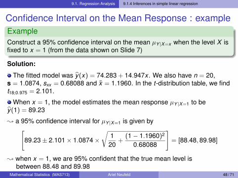
Confidence Interval on the Mean Response : exampleExampleConstruct a 95% confidence interval on the mean µY |X=x when the level X isfixed to x = 1 (from the data shown on Slide 7)
Solution:
The fitted model was y(x) = 74.283 + 14.947x . We also have n = 20,s = 1.0874, sxx = 0.68088 and x = 1.1960. In the t-distribution table, we findt18;0.975 = 2.101.
When x = 1, the model estimates the mean response µY |X=1 to bey(1) = 89.23
; a 95% confidence interval for µY |X=1 is given by[89.23± 2.101× 1.0874×
√120
+(1− 1.1960)2
0.68088
]= [88.48,89.98]
; when x = 1, we are 95% confident that the true mean level isbetween 88.48 and 89.98
Mathematical Statistics (MAS713) Ariel Neufeld 48 / 71
9.1. Regression Analysis 9.1.4 Inferences in simple linear regression
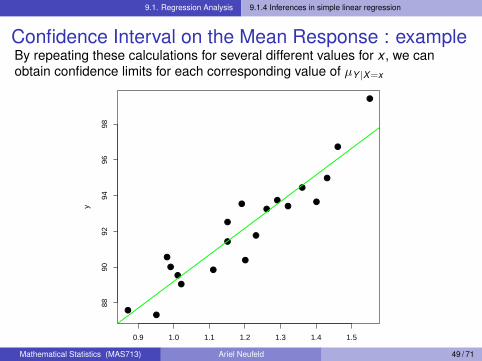
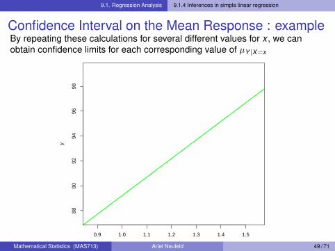
Confidence Interval on the Mean Response : exampleBy repeating these calculations for several different values for x , we canobtain confidence limits for each corresponding value of µY |X=x
●
●
●
●
●
●
●
●
●
●●
●
●
●●
●
● ●
●
●
0.9 1.0 1.1 1.2 1.3 1.4 1.5
8890
9294
9698
x
y
Mathematical Statistics (MAS713) Ariel Neufeld 49 / 71
9.1. Regression Analysis 9.1.4 Inferences in simple linear regression
Confidence Interval on the Mean Response : exampleBy repeating these calculations for several different values for x , we canobtain confidence limits for each corresponding value of µY |X=x
0.9 1.0 1.1 1.2 1.3 1.4 1.5
8890
9294
9698
x
y
Mathematical Statistics (MAS713) Ariel Neufeld 49 / 71

9.1. Regression Analysis 9.1.4 Inferences in simple linear regression
Confidence Interval on the Mean Response : exampleBy repeating these calculations for several different values for x , we canobtain confidence limits for each corresponding value of µY |X=x
0.9 1.0 1.1 1.2 1.3 1.4 1.5
8890
9294
9698
x
y
estimated regression lineconfidence limits
Mathematical Statistics (MAS713) Ariel Neufeld 49 / 71
9.1. Regression Analysis 9.1.5 Prediction of new observations
Prediction of new observations
Mathematical Statistics (MAS713) Ariel Neufeld 50 / 71

9.1. Regression Analysis 9.1.5 Prediction of new observations
Prediction of new observationsAn important application of a regression model is predicting new orfuture observations Y corresponding to a specified level X = x
; different to estimating the mean response µY |X=x at X = x !
From the model, the predictor of the new value of the response Y atX = x , say Y ∗(x) is naturally given by
Y ∗(x) = β0 + β1x ,
for which a predicted value is
y(x) = b0 + b1x
once the model has been fitted from an observed sample; the predictor of Y at X = x is the estimator of µY |X=x !The prediction error e is given by Y |(X = x)− Y ∗(x) and is normallydistributed, as both Y |(X = x) and Y ∗(x) are
Mathematical Statistics (MAS713) Ariel Neufeld 51 / 71
9.1. Regression Analysis 9.1.5 Prediction of new observations
Prediction of new observationsAs Y |(X = x) ∼ N (β0 + β1x , σ) (Slide 12) and
Y ∗(x) = µY |X=x ∼ N(β0 + β1x , σ
√1n + (x−x)2
sxx
)(Slide 46), the
expectation of the prediction error is
E((Y |(X = x))− Y ∗(x)) = E(Y |X = x)− E(Y ∗(x)) = 0
; on the average, the predictor will find the right value
Because the future Y is independent of the sample observations(and thus independent of µY |X=x ), the variance of prediction error is
Var((Y |(X = x))− Y ∗(x)) = Var(Y |X = x) + Var(Y ∗(x))
= σ2 + σ2(
1n + (x−x)2
sxx
)= σ2
(1 + 1
n + (x−x)2
sxx
)and we find
e := (Y |(X = x))− Y ∗(x) ∼ N
0, σ
√1 +
1n
+(x − x)2
sxx
Mathematical Statistics (MAS713) Ariel Neufeld 52 / 71

9.1. Regression Analysis 9.1.5 Prediction of new observations
Prediction of new observationsStandardising and replacing the unknown σ by its estimator S, we
get (as usual) :(Y |(X = x))− Y ∗(x)
S√
1 + 1n + (x−x)2
sxx
∼ tn−2
which directly leads to the following prediction interval for a newobservation Y , given that X = x :
Given data (x1, y1), . . . , (xn, yn)
=⇒ we find s and y(x) from the fitted model y(x) = b0 + b1x ,=⇒ a two-sided 100× (1− α)% prediction interval
for a new observation Y at X = x isy(x)− tn−2;1−α/2s
√1 +
1n
+(x − x)2
sxx, y(x) + tn−2;1−α/2s
√1 +
1n
+(x − x)2
sxx
Mathematical Statistics (MAS713) Ariel Neufeld 53 / 71

9.1. Regression Analysis 9.1.5 Prediction of new observations
Prediction of new observations : remarksSimilarly to the remarks on Slides 109–111 of Chapter 4, we observe :
1 a prediction interval for Y at X = x will always be longer than theconfidence interval for µY |X=x because there is much morevariability in one observation than in an average
Concretely, µY |X=x is the position of the straight line at X = x; the CI for µY |X=x only targets that position
However, we know that observations will not be exactly on thatstraight line, but ‘around’ it; a prediction interval for a new observation should take this
extra variability into account, in addition to the uncertaintyinherent in the estimation of µY |X=x
2 as n gets larger (n→∞), the width of the CI for µY |X=x decreasesto 0 (we are more and more accurate when estimating µ), but thisis not the case for the prediction interval : the inherent variability inthe new observation never vanishes, even when we haveobserved many other observations before!
Mathematical Statistics (MAS713) Ariel Neufeld 54 / 71

9.1. Regression Analysis 9.1.5 Prediction of new observations
Prediction of new observations : exampleExampleConstruct a 95% prediction interval on Y when the level X is fixed to x = 1%(from the data shown on Slide 4)
Solution:
The fitted model was y(x) = 74.283 + 14.947x . We also have n = 20,s = 1.0874, sxx = 0.68088 and x = 1.1960. In the t-distribution table, we findt18;0.975 = 2.101.
For x = 1, the model estimates the mean response µY |X=1 to y(1) = 89.23
; a 95% prediction interval for Y is given by[89.23± 2.101× 1.0874×
√1 +
120
+(1− 1.1960)2
0.68088
]= [86.83,91.63]
; if we fix the x = 1%, we can be 95% confident thatthe next observed value of y will be between 86.83 and 91.63
Mathematical Statistics (MAS713) Ariel Neufeld 55 / 71

9.1. Regression Analysis 9.1.5 Prediction of new observations
Prediction of new observations : exampleBy repeating these calculations for several different values for x , we canobtain prediction limits for each corresponding value of Y given that X = x
●
●
●
●
●
●
●
●
●
●●
●
●
●●
●
● ●
●
●
0.9 1.0 1.1 1.2 1.3 1.4 1.5
8890
9294
9698
x
y
estimated regression lineconfidence limitsprediction limits
Mathematical Statistics (MAS713) Ariel Neufeld 56 / 71

9.1. Regression Analysis 9.1.5 Prediction of new observations
Adequacy of the regression model
Mathematical Statistics (MAS713) Ariel Neufeld 57 / 71

9.1. Regression Analysis 9.1.6 Adequacy of the regression model
Adequacy of the regression model
While using the simple linear regression model, we made severalassumptions
The first one is that the model is correct : there indeed existcoefficients β0 and β1, as well as a random variable ε, such that wecan write Y = β0 + β1X + ε ; scatterplot
The other central assumption is certainly that (Slide 12)
Yi |(Xi = xi)i.i.d.∼ N (β0 + β1xi , σ) for i = 1,2, . . . ,n,
which has several implications
Mathematical Statistics (MAS713) Ariel Neufeld 58 / 71

9.1. Regression Analysis 9.1.6 Adequacy of the regression model
Adequacy of the regression model
Define the error terms
ei = yi − (β0 + β1xi), for i = 1, . . . ,n
which are values drawn from the distribution of ε. We must check that :1 the ei ’s have been drawn independently of one another2 the ei ’s have been drawn from a distribution with the same
variance3 the ei ’s have been drawn from a normal distribution
Mathematical Statistics (MAS713) Ariel Neufeld 59 / 71
9.1. Regression Analysis 9.1.6 Adequacy of the regression model
Residual analysis
Unfortunately, we do not have access to the values ei ’s (as we do notknow β0 and β1)
However, the observed residuals of the fitted model
ei = yi − y(xi) = yi − (b0 + b1xi)
are probably good estimates of those ei ’s ; residual analysis
Mathematical Statistics (MAS713) Ariel Neufeld 60 / 71

9.1. Regression Analysis 9.1.6 Adequacy of the regression model
Residual analysis
It is frequently helpful to plot the residuals
(1) in time sequence (if known),
(2) against the fitted values y(xi), and
(3) against the predictor values xi
Typically, these graphs will look like one of the four general patternsshown on the next slide
As suggested by their name, the residuals are everything the modelwill not consider ; no information should be observed in the residuals,they should look like noise
Mathematical Statistics (MAS713) Ariel Neufeld 61 / 71

9.1. Regression Analysis 9.1.6 Adequacy of the regression model
Residual analysis
●
●
●
●●
●●
●
●
●
●
●
●
●●
●
●
●
●
●
●
●
●
●
●
●
●
●
●
●
●
●
●
●
●
●
●
●
●
●
● ●●
●
●
●
●
●
●
●
(a)
e i
0 ●
● ●
●
●
●●●
●
●
●
● ●●
●
●
●
●
●
●●
●
●
●
●
●
●
●
●
●
●
●
●
●
●●
●
●
●
●
● ●●
●
●
●
●
● ●
●
(b)
e i
0
●
●
●
●
●
●
●
●
● ●
●
●
●●
●
●●●
●
●
●
●
●
●
●
●
●
●
●
●
●●
●
●
●
●
● ●
●
●
●
●
●
●
●
●
●
●
●
●
(c)
e i
0
●
●
●●
●●
●●
● ●
●
●
●
●
●
●
●
●
●
●●
●
●
●
●
●
●
●
●
●
●●
●
●●
●
●●
●
●
●
●
●
●
●
●
●
●
●
●
(d)
e i
0
Mathematical Statistics (MAS713) Ariel Neufeld 62 / 71
9.1. Regression Analysis 9.1.6 Adequacy of the regression model
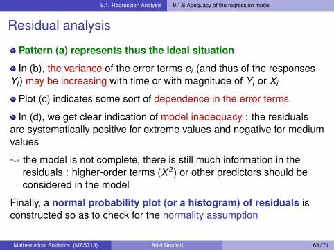
Residual analysis
Pattern (a) represents thus the ideal situation
In (b), the variance of the error terms ei (and thus of the responsesYi ) may be increasing with time or with magnitude of Yi or Xi
Plot (c) indicates some sort of dependence in the error terms
In (d), we get clear indication of model inadequacy : the residualsare systematically positive for extreme values and negative for mediumvalues
; the model is not complete, there is still much information in theresiduals : higher-order terms (X 2) or other predictors should beconsidered in the model
Finally, a normal probability plot (or a histogram) of residuals isconstructed so as to check for the normality assumption
Mathematical Statistics (MAS713) Ariel Neufeld 63 / 71
9.1. Regression Analysis 9.1.6 Adequacy of the regression model
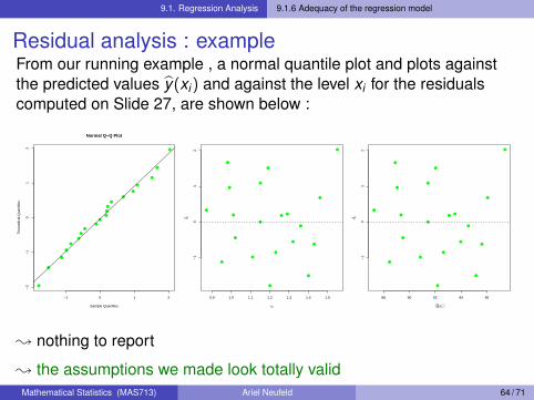
Residual analysis : exampleFrom our running example , a normal quantile plot and plots againstthe predicted values y(xi) and against the level xi for the residualscomputed on Slide 27, are shown below :
●
●
●
●
●
●
●
●
●
●
●
●
●
●
●
●
●
●
●
●
−1 0 1 2
−2
−1
01
2
Normal Q−Q Plot
Sample Quantiles
The
oret
ical
Qua
ntile
s
●
●
●
●
●
●
●
●
●
●
●
●
●
●
●
●
●
●●
●
0.9 1.0 1.1 1.2 1.3 1.4 1.5
−1
01
2
xi
e i●
●
●
●
●
●
●
●
●
●
●
●
●
●
●
●
●
●●
●
88 90 92 94 96
−1
01
2
y(xi)
e i
; nothing to report
; the assumptions we made look totally validMathematical Statistics (MAS713) Ariel Neufeld 64 / 71

9.1. Regression Analysis 9.1.6 Adequacy of the regression model
Variability decompositionSimilarly to the notations on Slide 20, we can define
syy =n∑
i=1
(yi − y)2
; this measures the total amount of variability in the response values,and is sometimes denoted sst (for ‘total sum of squares’)
Now, this variability in the observed values yi arises from two factors :1 because the xi values are different, all Yi have different means. This
variability is quantified by the ‘regression sum of squares’ :
ssr =n∑
i=1
(y(xi )− y)2
2 each value Yi has variance σ2 around its mean. This variability isquantified by the ‘error sum of squares’ :
sse =n∑
i=1
(yi − y(xi ))2 =n∑
i=1
e2i
We can always write : sst = ssr + sse
Mathematical Statistics (MAS713) Ariel Neufeld 65 / 71

9.1. Regression Analysis 9.1.6 Adequacy of the regression model
Coefficient of determinationSuppose sst ' ssr and sse ' 0 : the variability in the responses due tothe effect of the predictor is almost the total variability in the responses
; concretely, all the dots are very close to the straight line : the linearregression model fits the data very well
Now suppose that sst ' sse and ssr ' 0 : almost the whole variation inthe responses is due to the error terms
; the dots are very far away from the fitted straight line, the regressionmodel is merely useless
; comparing ssr to sst allows to judge the adequacy of the model
The quantity r2, called the coefficient of determination, defined by
r2 =ssr
sst,
represents the proportion of the variability in the responses that isexplained by the predictor
Mathematical Statistics (MAS713) Ariel Neufeld 66 / 71

9.1. Regression Analysis 9.1.6 Adequacy of the regression model
Coefficient of determinationClearly, the coefficient of variation will have a value between 0 and 1 :
a value of r2 near 1 indicates a good fit to the dataa value of r2 near 0 indicates a poor fit to the data
FactIf the regression model is able to explain most of the variation in theresponse data, then it is considered to fit the data well, and is regardedas a ‘good’ model
In our running example, we find in the regression output on Slide 25 avalue of r2 (R-Sq) equal to 87.74%
; almost 88% of the variation of y thelevel was used. The remaining 12% of thevariation is due to the natural variability
Here r2 is quite close to 1, which makes our model quite reliableMathematical Statistics (MAS713) Ariel Neufeld 67 / 71

9.1. Regression Analysis 9.1.7 Correlation
Correlation
Mathematical Statistics (MAS713) Ariel Neufeld 68 / 71

9.1. Regression Analysis 9.1.7 Correlation
CorrelationOn Slide 18 of Chapter 3.4, we introduced the correlation coefficientbetween two random variables X and Y :
ρ =Cov(X ,Y )√Var(X )Var(Y )
This coefficient quantifies the strength of the linear relationshipbetween X and Y
; if ρ is close to 1 or −1, there is a strong linear relationship betweenX and Y
; observations in a random sample {(xi , yi), i = 1, . . . ,n} drawn from(X ,Y ) should fall close to a straight line
; a linear regression model linking Y to X , based on that sample,should be a good model, with a value of r2 close to 1
; trueMathematical Statistics (MAS713) Ariel Neufeld 69 / 71

9.1. Regression Analysis 9.1.7 Correlation
CorrelationWe can write :
r2 =ssr
sst=
sst − sse
syy=
sxx (sst − sse)
sxxsyy=
s2xy
sxxsyy
=(∑
i (xi − x)(yi − y))2∑i (xi − x)2
∑i (yi − y)2
; we observe that r =
∣∣∑i (xi − x)(yi − y)
∣∣√∑i (xi − x)2
∑i (yi − y)2
; except for its sign (positive or negative linear relationship), thesample correlation is the square root of the coefficient of determination(its sign is the sign of b1)
In our running example, the sample correlation coefficient is√0.8774 = 0.9366 (good estimate of the ‘true’ correlation coefficient between
x level and y )
Mathematical Statistics (MAS713) Ariel Neufeld 70 / 71

9.1. Regression Analysis Objectives
ObjectivesNow you should be able to :
Use simple linear regression for building models to engineeringand scientific dataUnderstand how the method of least squares is used to estimatethe regression parametersAnalyse residuals to determine if the regression model is anadequate fit to the data and to see if any underlying assumptionsis violatedTest statistical hypotheses and construct confidence intervals onregression parametersUse the regression model to make a prediction of a futureobservation and construct an appropriate prediction intervalUnderstand how the linear regression model and the correlationcoefficient are related
Mathematical Statistics (MAS713) Ariel Neufeld 71 / 71