MATHEMATICA SOLUTIONS TO THE CHEMICAL ENGINEERING … · MATHEMATICA SOLUTIONS TO THE CHEMICAL...
63
MATHEMATICA SOLUTIONS TO THE CHEMICAL ENGINEERING PROBLEM SET 1 H. Eric Nuttall Department of Chemical/Nuclear Engineering Farris Engineering Center, Rm 209 University of New Mexico Albuquerque, New Mexico 87131-1341 INTRODUCTION These solutions are for a set of numerical problems in chemical engineering. Professor Michael B. Cutlip of the University of Connecticut developed the problems and Professor Mordechai Shacham of Ben-Gurion University of the Negev for the ASEE Chemical Engineering Summer School held in Snowbird, Utah in August, 1997. The problem statements are provided in another document. 1 Professors Cutlip and Shacham provided a document that showed how to solve the problems using POLYMATH. Professor H. Eric Nuttall of the University of New Mexico provided solutions using Mathematica and Professor J. J. Hwalek provided solutions using Mathcad. After the conference, Professor Ross Taylor provided solutions in Maple, and Edward Rosen provided solution in EXCEL. This paper gives the solutions in MATHEMATICA version 3.0. All documents and solutions are available from http://www.che.utexas.edu/cache/ and via FTP from ftp.engr.uconn.edu/pub/ASEE. The written materials are only readable in Adobe Acrobat 3.0 format and higher; however, this software is free via the Internet from www.adobe.com. The MATHEMATICA solutions were derived using version 3.0. This version of MATHEMATICA is the same on all platforms; hence, the notebooks should work the same for all users independent of computer model. MATHEMATICA is a very extensive and comprehensive computational tool; hence, there are several possible approaches and various routines in MATHEMATICA available for solving each of the ten problems. The approach chosen here is that of the author which means other solutions may prove to be better. Also please note that in addition to using the routines provided by MATHEMATICA one can easily write there own programs/functions. This programming capability greatly extends the usefulness of MATHEMATICA. Numerous primers and publications are available to instruct the user on the operation of MATHEMATICA. Also the online help system is very comprehensive and includes numerous examples for each command. I have found MATHEMATICA to be an indispensable computational tool for teaching and solving engineering problems. All of our Ch.E. students at the University of New Mexico know and use MATHEMATICA. This prefer this package overall the others which are also equally available to the students. 1 “The Use of Mathematica Software packages in Chemical Engineering”. Michael B. Cutlip, John J. Hwalek, H. Eric Nuttall, Mordechai Shacham, Workshop from Session 12, Chemical Engineering Summer School, Snowbird, Utah, Aug., 1997. M i
Transcript of MATHEMATICA SOLUTIONS TO THE CHEMICAL ENGINEERING … · MATHEMATICA SOLUTIONS TO THE CHEMICAL...

MATHEMATICA SOLUTIONS TO THE CHEMICALENGINEERING PROBLEM SET1
H. Eric NuttallDepartment of Chemical/Nuclear Engineering
Farris Engineering Center, Rm 209University of New Mexico
Albuquerque, New Mexico 87131-1341
INTRODUCTION
These solutions are for a set of numerical problems in chemical engineering.Professor Michael B. Cutlip of the University of Connecticut developed the problems andProfessor Mordechai Shacham of Ben-Gurion University of the Negev for the ASEEChemical Engineering Summer School held in Snowbird, Utah in August, 1997. Theproblem statements are provided in another document.1 Professors Cutlip and Shachamprovided a document that showed how to solve the problems using POLYMATH.Professor H. Eric Nuttall of the University of New Mexico provided solutions usingMathematica and Professor J. J. Hwalek provided solutions using Mathcad. After theconference, Professor Ross Taylor provided solutions in Maple, and Edward Rosenprovided solution in EXCEL. This paper gives the solutions in MATHEMATICA version3.0. All documents and solutions are available from http://www.che.utexas.edu/cache/ andvia FTP from ftp.engr.uconn.edu/pub/ASEE. The written materials are only readable inAdobe Acrobat 3.0 format and higher; however, this software is free via the Internet fromwww.adobe.com.
The MATHEMATICA solutions were derived using version 3.0. This version ofMATHEMATICA is the same on all platforms; hence, the notebooks should work thesame for all users independent of computer model. MATHEMATICA is a very extensiveand comprehensive computational tool; hence, there are several possible approaches andvarious routines in MATHEMATICA available for solving each of the ten problems. Theapproach chosen here is that of the author which means other solutions may prove to bebetter. Also please note that in addition to using the routines provided byMATHEMATICA one can easily write there own programs/functions. This programmingcapability greatly extends the usefulness of MATHEMATICA. Numerous primers andpublications are available to instruct the user on the operation of MATHEMATICA. Alsothe online help system is very comprehensive and includes numerous examples for eachcommand. I have found MATHEMATICA to be an indispensable computational tool forteaching and solving engineering problems. All of our Ch.E. students at the University ofNew Mexico know and use MATHEMATICA. This prefer this package overall the otherswhich are also equally available to the students.
1 “The Use of Mathematica Software packages in Chemical Engineering”. Michael B.Cutlip, John J. Hwalek, H. Eric Nuttall, Mordechai Shacham, Workshop from Session 12,Chemical Engineering Summer School, Snowbird, Utah, Aug., 1997.
M i

1. Molar Volume and Compressibility Factor from Van Der Waals Equation
Mathematica
Mathematica has its own notebook interface which works somewhat as a wordprocessor but allows mathematical operations directly within the notebook. In addition, it uses the concept of built in or user written functions to perform the mathematical tasks. Note that in these notebooks the gray sections are input and the next line will be output. Mathematica has a good on-line help utility but to learn how to effectively use this application it is best to read one of the many help books such as: Nancy Blachman, Mathematica: A Practical Approach, Prentice Hall. A new edition for Mathematica version 3.0 will be available soon.
� Mathematica--Define equation, paramters and functions
H* define all the constants used in the equation andthe compressibility factor as a function. Note itis possible to include units with the constantsbut this was not done in these problems. *L
R = 0.08206; Tc = 405.5; Pc = 111.3; Pr@P_D := P � Pc;a = 27 HR^2 Tc^2 �PcL� 64; b = R Tc � H8 PcL;Z@P_, V_, T_D := P V � HR TL; T =.; P =.;
H* van der Waals equation *Leqn = HP + a � V^2L HV - bL == R T
JP +4.19695�����������������������
V2N H-0.0373712 + VL == 0.08206 T
Mathematica ASEE Session 12--Problem 1 M 1

� Part (a)--Calculate the molar volume and compressibility factor for gaseous ammonia at a pressure of P=56 atm and a temperature of T=450 K using the van der Waals equation of state.
H* temperature and pressure *L
T = 450; P = 56;
H* Solve vad der Waals equation *L
FindRoot@eqn, 8V, 0.57<D
8V ® 0.574892<
H* evaluate compressibility factor *L
Z@P, 0.574892, TD
0.871827
� Part (b)--Repeat the problem for a series of reduced pressures: Pr=1,2,4,10, and 20
H* Define partial pressures in the array Pr *L
Pr@0D = 0.503; Pr@1D = 1; Pr@2D = 2; Pr@3D = 4;Pr@4D = 10; Pr@5D = 20;
Mathematica ASEE Session 12--Problem 1 M 2

H* Create table of P, Pr V and Z *L
TableForm@Table@8P = Pr@iD Pc,Pr@iD, V1 = V �. FindRoot@eqn, 8V, 0.56<D,Z@P, V1, TD<, 8i, 0, 5<D,
TableHeadings -> 8None, 8"PHatmL", "Pr", "V", "Z"<<,TableAlignments -> CenterD
PHatmL Pr V Z55.9839 0.503 0.575084 0.871868
111.3 1 0.233509 0.703808
222.6 2 0.0772676 0.465777
445.2 4 0.0606543 0.731261
1113. 10 0.0508753 1.53341
2226. 20 0.046175 2.78348
� Part (c)--Generate a table and plot Pr versus Z
plist = Table@8Pr@iD,Z@P = Pr@iD Pc, V �. FindRoot@eqn, 8V, 0.56<D, TD<,
8i, 0, 5<D
880.503, 0.871868<, 81, 0.703808<, 82, 0.465777<,84, 0.731261<, 810, 1.53341<, 820, 2.78348<<
TableForm@plist, TableHeadings -> 8None, 8"Pr", "Z"<<,TableAlignments -> CenterD
Pr Z0.503 0.871868
1 0.703808
2 0.465777
4 0.731261
10 1.53341
20 2.78348
Mathematica ASEE Session 12--Problem 1 M 3

ListPlot@plist, PlotRange -> 880, 20<, 80, 3<<,PlotStyle -> [email protected],Frame -> True, GridLines -> AutomaticD
2.5 5 7.5 10 12.5 15 17.5 20
0.5
1
1.5
2
2.5
3
� Graphics �
Mathematica ASEE Session 12--Problem 1 M 4

2. Steady Steate Material Balances on a Separation Train
Mathematica
à This set of simultaneous linear algebraic equations can be solved directly using the "Solve" function in Mathematica. There are other linear equation solving routines in Mathematica that could be used for larger sets of simultaneous equations and of course, matrix algebra approach could be used as well. But the method shown is the most common routine and approach in Mathematica for solving equations. Since Mathematica is a symbolic program one can assign the equations equal to variables to simplicity and clarification.
à Part (a) Solve the set of linear simultaneous equations for the unknowns: D1, D2, B1, B2.
H* Xylene*LeqnX = 0.07 D1 + 0.18 B1 + 0.15 D2 + 0.24 B2 == 0.15 * 70;H* Styrene*LeqnS = 0.04 D1 + 0.24 B1 + 0.1 D2 + 0.65 B2 == 0.25 *70;H* Touene *LeqnT = 0.54 D1 + 0.42 B1 + 0.54 D2 + 0.1 B2 == 0.4 * 70;H* Benzene*LeqnB = 0.35 D1 + 0.16 B1 + 0.21 D2 + 0.01 B2 == 0.2 *70;
Mathematica ASEE Session 12--Problem 2 M 5

answers =Solve@8eqnX, eqnS, eqnT, eqnB<, 8D1, B1, D2, B2<D
H* Answers appear in the rule construct. Thisrule construct makes symbolic programs verypowerful. The rule construct will appear inmany of the problem solutions. *L
88D1 ® 26.25, B1 ® 17.5, D2 ® 8.75, B2 ® 17.5<<
� This step shown below reduces the answer list from a list of lists to a simple list for use in Part (b). Notice that there are one less set of braces around the list!
answers = Part@answers, 1D
8D1 ® 26.25, B1 ® 17.5, D2 ® 8.75, B2 ® 17.5<
à Part (b)-Solve for compositions and molar flow rates in streams B & D
� Part (b)--Equations (again for convenience and clarity the equations are assigned to variables)
eqn1 = D == D1 + B1;eqn2 = XDx D == 0.07 D1 + 0.18 B1;eqn3 = XDs D == 0.04 D1 + 0.24 B1;eqn4 = XDt D == 0.54 D1 + 0.42 B1;eqn5 = XDb D == 0.35 D1 + 0.16 B1;eqn6 = B == D2 + B2;eqn7 = XBx B == 0.15 D2 + 0.24 B2;eqn8 = XBs B == 0.1 D2 + 0.65 B2;eqn9 = XBt B == 0.54 D2 + 0.1 B2;eqn10 = XBb B == 0.21 D2 + 0.01 B2;
Mathematica ASEE Session 12--Problem 2 M 6

H* Again the "Solve " function is used.It is necessary to substitute into theequations the solutions from Part HaL. *L
answers2 = Solve@ReplaceAll@8eqn1, eqn2, eqn3, eqn4, eqn5, eqn6, eqn7,eqn8, eqn9, eqn10<, answersD,8D, B, XDx, XDs, XDt, XDb, XBx, XBs, XBt, XBb<D
88XDx ® 0.114, XDs ® 0.12, XDt ® 0.492, XDb ® 0.274, XBx ® 0.21,XBs ® 0.466667, XBt ® 0.246667, XBb ® 0.0766667,B ® 26.25, D ® 43.75<<
H* The answers from Part HbL arelisted in the rule construct as a table *L
Part@answers2, 1D �� TableForm
XDx ® 0.114
XDs ® 0.12
XDt ® 0.492
XDb ® 0.274
XBx ® 0.21
XBs ® 0.466667
XBt ® 0.246667
XBb ® 0.0766667
B ® 26.25
D ® 43.75
Mathematica ASEE Session 12--Problem 2 M 7

3. Vapor Pressure Data Representaton by Polynomials and Equations
Mathematica
In this problem the same temperature versus pressure data is fit using three different models, i.e.,1) a polynomial with increasing order--linear regression2) the Clausiu-Clapeyron equation--linear regression of transformed data3) the Antoine equation--nonlinear regression or curve fitting
In each case, the final model and data are graphed on the same plot for comparison.
à Part (a)--polynomial fit
� Define the regression data--Temperature (C) versus P (mm Hg)
data = 88-36.7, 1<, 8-19.6, 5<, 8-11.5, 10<, 8-2.6, 20<,87.6, 40<, 815.4, 60<, 826.1, 100<, 842.2, 200<,860.6, 400<, 880.1, 760<<
88-36.7, 1<, 8-19.6, 5<, 8-11.5, 10<, 8-2.6, 20<,87.6, 40<, 815.4, 60<, 826.1, 100<, 842.2, 200<,860.6, 400<, 880.1, 760<<
Mathematica ASEE Session 12--Problem 3 M 8

data �� TableForm H* T versus P *L
-36.7 1
-19.6 5
-11.5 10
-2.6 20
7.6 40
15.4 60
26.1 100
42.2 200
60.6 400
80.1 760
H* Plot T versus P *L
p1 = ListPlot@data, PlotStyle -> [email protected],PlotRange -> 88-50, 100<, 80, 800<<,AxesOrigin -> 8-50, 0<D
� Graphics �
� Part (a) Regress the data with a increasing orders of a polynamial in P. Analyze the R squared for best fit.
H* add a standardMathematica package to the kernal *L
Needs@"Statistics`LinearRegression`"D
Mathematica ASEE Session 12--Problem 3 M 9

H* first order polynomial in T,RSquared=0.78 *L
T =.;Hregress = Regress@data, 81, T<, TD;
Chop@regress, 10^H-6LDL
9ParameterTable ®
Estimate SE TStat PValue
1 64.406 42.4524 1.51713 0.167708
T 5.89072 1.10667 5.32294 0.000708522
,RSquared ® 0.779819,AdjustedRSquared ® 0.752296,EstimatedVariance ® 14823.8, ANOVATable ®
DF SumOfSq MeanSq FRatio PValue
Model 1 420014. 420014. 28.3337 0.00070
Error 8 118591. 14823.8
Total 9 538604.
=
Mathematica ASEE Session 12--Problem 3 M 10

H* Second order polynomial in T,RSquared=0.98 *L
regress = Regress@data, 81, T, T^2<, TD;Chop@regress, 10^H-6LD
9ParameterTable ®
Estimate SE TStat PValue
1 -0.582065 13.9506 -0.0417234 0.967884
T 2.06715 0.511995 4.03744 0.00494892
T2 0.0861526 0.00905805 9.51116 0.00002974
,RSquared ® 0.984186,AdjustedRSquared ® 0.979668,EstimatedVariance ® 1216.79, ANOVATable ®
DF SumOfSq MeanSq FRatio PValue
Model 2 530087. 265043. 217.823 0
Error 7 8517.5 1216.79
Total 9 538604.
=
Mathematica ASEE Session 12--Problem 3 M 11

H* Third order polynomial in T,RSquared=0.9996-- This is a very good fit *L
regress = Regress@data, 81, T, T^2, T^3<, TD;Chop@regress, 10^H-6LD
9ParameterTable ®
Estimate SE TStat PValue
1 24.4594 2.83402 8.63062 0.0001332
T 1.1981 0.102232 11.7195 0.0000232
T2 0.0394481 0.0033548 11.7587 0.0000228
T3 0.000744911 0.0000477255 15.6082 4.3796 ´ 1
,RSquared ® 0.99962,AdjustedRSquared ® 0.99943,EstimatedVariance ® 34.1222, ANOVATable ®
DF SumOfSq MeanSq FRatio PValue
Model 3 538400. 179467. 5259.52 0
Error 6 204.733 34.1222
Total 9 538604.
=
H* In this statement the final polynomial isgenerated in order to graph the function *L
eqn1 = Fit@data, 81, T, T^2, T^3<, TD
24.4594 + 1.1981 T + 0.0394481 T2 + 0.000744911 T3
Mathematica ASEE Session 12--Problem 3 M 12

H* This is a fancy way to overlaythe data onto the polynomial function *L
p2 = Plot@eqn1, 8T, -50, 100<,Epilog ® [email protected], Point��data<D
-40 -20 20 40 60 80 100
200
400
600
800
1000
1200
� Graphics �
à Part (b) Regression with Clausius-Clapeyron Equation
data
88-36.7, 1<, 8-19.6, 5<, 8-11.5, 10<, 8-2.6, 20<,87.6, 40<, 815.4, 60<, 826.1, 100<, 842.2, 200<,860.6, 400<, 880.1, 760<<
Mathematica ASEE Session 12--Problem 3 M 13

� In this next operation the data is transformed to temperature versus log10 of pressure
H* Take the log10 of each pressure *L
Transdata =Table@8First@data@@iDDD,Log@10, Last@data@@iDDDD<, 8i, 10<D �� N
88-36.7, 0<, 8-19.6, 0.69897<, 8-11.5, 1.<,8-2.6, 1.30103<, 87.6, 1.60206<, 815.4, 1.77815<,826.1, 2.<, 842.2, 2.30103<, 860.6, 2.60206<,880.1, 2.88081<<
H* Regress the transformeddata and generate an equation model *L
CCmodel = Fit@Transdata, 81, -1� HT + 273.15L<, TD
8.75201 -2035.33
����������������������������273.15 + T
H* Transform data forgraphing to 1�H273.15+TL vs. Log10 HPL *L
plotdata = Table@81000 * 1� H273.15 + First@data@@iDDDL,Log@10, Last@data@@iDDDD<, 8i, 1, 10<D ��
N
884.22922, 0<, 83.944, 0.69897<,83.8219, 1.<, 83.69617, 1.30103<, 83.56189, 1.60206<,83.4656, 1.77815<, 83.34169, 2.<, 83.17108, 2.30103<,82.99625, 2.60206<, 82.83086, 2.88081<<
Mathematica ASEE Session 12--Problem 3 M 14

H* Plot Clausius-Clapayron model and transformed data *L
[email protected] - 2035.331 * invTK � 1000,8invTK, 2.6, 4.3<, PlotRange -> 882.6, 4.6<, 80, 3<<,AxesOrigin -> 82.6, 0<,
Epilog ® [email protected], Point��plotdata<D
2.75 3 3.25 3.5 3.75 4 4.25 4.5
0.5
1
1.5
2
2.5
3
� Graphics �
à Part (c) Regression with the Antoine Equation
H* load into Mma kernal the standard package *L
<< Statistics`NonlinearFit`
T =.;NonlinearFit@Transdata, A - B �HT + CL, T, 88A, 5<, 8B, 600<, 8C, 150<<D
5.64228 -637.031
��������������������������������149.198 + T
Mathematica ASEE Session 12--Problem 3 M 15

NonlinearRegress@Transdata, A - B � HT + CL, T,88A, 5<, 8B, 600<, 8C, 150<<D
9BestFitParameters ®
8A ® 5.64228, B ® 637.031, C ® 149.198<, ParameterCITable ®
Estimate Asymptotic SE CI
A 5.64228 0.133415 85.3268, 5.95776<
B 637.031 41.7901 8538.213, 735.849<
C 149.198 4.98397 8137.413, 160.983<
,
EstimatedVariance ® 0.00036253, ANOVATable ®
DF SumOfSq MeanSqModel 3 33.2717 11.0906
Error 7 0.0025377 0.00036253
Uncorrected Total 10 33.2742
Corrected Total 9 7.14634
,
AsymptoticCorrelationMatrix ®i
k
jjjjjjj
1. 0.993145 0.975547
0.993145 1. 0.994079
0.975547 0.994079 1.
y
{
zzzzzzz,
FitCurvatureTable ®
Curvature
Max Intrinsic 0.020214
Max Parameter-Effects 2.44175
95. % Confidence Region 0.479638
=
Mathematica ASEE Session 12--Problem 3 M 16

à The above values for A, B, and C differ from those calculated by Polymath. Below I set C equal to the Polymath value (153.885) and calculated A and B. This procedure gave the same results as Polymath.
H* Values for A and Bthe same as calculated from Polymath *L
NonlinearRegress@Transdata, A - B �HT + 153.885L, T, 8A, B<D
9BestFitParameters ® 8A ® 5.76734, B ® 677.091<, ParameterCITable ®
Estimate Asymptotic SE CI
A 5.76734 0.0264636 85.70631, 5.82836<
B 677.091 4.22989 8667.337, 686.845<
,
EstimatedVariance ® 0.000278812, ANOVATable ®
DF SumOfSq MeanSqModel 2 33.272 16.636
Error 8 0.0022305 0.000278812
Uncorrected Total 10 33.2742
Corrected Total 9 7.14634
,
AsymptoticCorrelationMatrix ® J1. 0.979892
0.979892 1.N,
FitCurvatureTable ®
Curvature
Max Intrinsic 0
Max Parameter-Effects 0
95. % Confidence Region 0.473568
=
Mathematica ASEE Session 12--Problem 3 M 17

à Below is a plot showing that the two solutions are essentially identical and that they fit the data very well.
H* Note that the Antonine equation with differentconstants gives essentially identical results *L
pc2 = PlotA
95.76734 -677.0908
��������������������������������������153.8849 + Tc
, 5.64227 -637.0310
�����������������������������������������149.19784 + Tc
=,
8Tc, -40, 80<E
-40 -20 20 40 60 80
0.5
1
1.5
2
2.5
� Graphics �
Mathematica ASEE Session 12--Problem 3 M 18

� Next the data is overlayed onto the Antoine equation
pc1 = ListPlot@Transdata, PlotStyle -> [email protected],PlotRange -> 88-60, 90<, 80, 3<<,AxesOrigin -> 8-60, 0<D
-40 -20 0 20 40 60 80
0.5
1
1.5
2
2.5
3
� Graphics �
Show@pc1, pc2DH* plot combined data and model results *L
-40 -20 0 20 40 60 80
0.5
1
1.5
2
2.5
3
� Graphics �
Mathematica ASEE Session 12--Problem 3 M 19

4. Reaction Equilibrium for Multiple Gas Phase Reactions
Mathematica
This problem requires the solution of simultaneous nonlinear algebraic equations. The Mathematica function FindRoot is used to solve these equations. Use the online help to learn more about the built-in FindRoot utility function.
Mathematica ASEE Session 12--Problem 4 M 20

� For the equations see the problem statement EQUATIONS (12)
� Setup equations for solving using MathematicaFindRoot function. Note that the numerical values for certain constants are given and assigned below along with the necessary equations.
f1 = Cc Cd - Kc1 Ca Cb == 0;f2 = Cx Cy - Kc2 Cb Cc == 0;f3 = Cz - Kc3 Ca Cx == 0;eqn4 = Ca == Ca0 - Cd - Cz;eqn5 = Cb == Cb0 - Cd - Cy;eqn6 = Cc == Cd - Cy;eqn7 = Cy == Cx + Cz;Ca0 = Cb0 = 1.5;Kc1 = 1.06;Kc2 = 2.63;Kc3 = 5;
à Parts-(a), (b) and (c)
à Solve using the three different starting values for CD, CX and CZ
� Trial #1
answera =FindRoot@8f1, f2, f3, eqn4, eqn5, eqn6, eqn7<, 8Ca, 1<,8Cb, 1<, 8Cc, 1<, 8Cd, 0<, 8Cx, 0<, 8Cy, 1<, 8Cz, 0<D
8Ca ® 0.420689, Cb ® 0.242897, Cc ® 0.153565,Cd ® 0.705334, Cx ® 0.177792, Cy ® 0.551769, Cz ® 0.373977<
Mathematica ASEE Session 12--Problem 4 M 21

� Trial #2
answerb =FindRoot@8f1, f2, f3, eqn4, eqn5, eqn6, eqn7<, 8Ca, 1<,8Cb, 1<, 8Cc, 1<, 8Cd, 1<, 8Cx, 1<, 8Cy, 1<, 8Cz, 1<D
8Ca ® 0.420689, Cb ® 0.242897, Cc ® 0.153565,Cd ® 0.705334, Cx ® 0.177792, Cy ® 0.551769, Cz ® 0.373977<
� Trial #3
answerc =FindRoot@8f1, f2, f3, eqn4, eqn5, eqn6, eqn7<, 8Ca, 1<,8Cb, 1<, 8Cc, 1<, 8Cd, 10<, 8Cx, 10<, 8Cy, 1<, 8Cz, 10<D
8Ca ® 0.420689, Cb ® 0.242897, Cc ® 0.153565,Cd ® 0.705334, Cx ® 0.177792, Cy ® 0.551769, Cz ® 0.373977<
� The table shown below lists the solutions from each trial. Note that they are all exactly the same.
Table@8answera@@iDD,answerb@@iDD, answerc@@iDD<, 8i, 1, 7<D ��
TableForm
Ca ® 0.420689 Ca ® 0.420689 Ca ® 0.420689
Cb ® 0.242897 Cb ® 0.242897 Cb ® 0.242897
Cc ® 0.153565 Cc ® 0.153565 Cc ® 0.153565
Cd ® 0.705334 Cd ® 0.705334 Cd ® 0.705334
Cx ® 0.177792 Cx ® 0.177792 Cx ® 0.177792
Cy ® 0.551769 Cy ® 0.551769 Cy ® 0.551769
Cz ® 0.373977 Cz ® 0.373977 Cz ® 0.373977
Mathematica ASEE Session 12--Problem 4 M 22

5. Terminal Velocity of Falling Particles
Mathematica
� Mathematica has many special capabilities. For this problem, user written conditional functions are used. The problem is nonlinear because the particle velocity appears both in the equation and embedded in the Reynolds number which appears in the drag coeficient equation. Hence a very nonlinear problem!
First, define the Drag Coefficient function for various ranges of Re using the conditional function construct.
CD@Re_D := 24 � Re �; Re < 0.1;CD@Re_D := H24� ReL H1 + 0.14 Re^0.7L �; 0.1 <= Re <= 1000;CD@Re_D := 0.44 �; 1000 < Re < 350000;
H* Reference for this specialconditional function construct: N. Blachman,Mathematica: A Practical Approach, pg. 170 *L
� Next define the parameters (given data) using the list & rule construct. This construct preserves the symbolic form of the equations.
data = 8r -> 994.6 , rp -> 1800, Ð -> 8.93 * 10^-4 ,Dp -> 0.208 * 10^-3, g -> 9.80665<
8r ® 994.6, rp ® 1800, Ð ® 0.000893, Dp ® 0.000208,g ® 9.80665<
Unprotect@ReD; H* if we wish to use the symbol"Re" we must unprotect it. In Mathematicathis symbol is already defined *L
Mathematica ASEE Session 12--Problem 5 M 23

� Define equations: Reynolds number and particle velocity
eqn1 = Re == Dp vt r � Ð
Re ==Dp vt r��������������������
Ð
eqn2 = vt == Sqrt@4 g Hrp - rL Dp � H3 CD@ReD rLD
vt ==
2 $
++++++++++++++++++++++++++Dp g H-r+rpL��������������������������
r CD@ReD
�����������������������������������������++++3
� Solve the nonlinear equations simultaneously-Part (a)
solution = FindRoot@Evaluate@8eqn1, eqn2< �. dataD,8Re, 81, 1000<<, 8vt, 80.01, 0.02<<D
8Re ® 3.65632, vt ® 0.0157828<
Mathematica ASEE Session 12--Problem 5 M 24

� Plot function velocity equation versus vt to graphically verify the calculated solution.
H* This plot is just a fun and visually instructiveway to see graphically the correct solution *L
Plot@vt - Sqrt@4 g Hrp - rL Dp �H3 CD@Dp vt r �ÐD rLD �. data �.data, 8vt, 0.000, 0.02<D
0.005 0.01 0.015 0.02
-0.004
-0.003
-0.002
-0.001
0.001
0.002
� Graphics �
� Summary of answers for Part (a)
Join@solution, 8CD -> CD@ReD �. solution<D �� ColumnForm
Re ® 3.65632
vt ® 0.0157828
CD ® 8.8413
Mathematica ASEE Session 12--Problem 5 M 25

à Part (b)--Recalculate the problem assuming gravity is 30 times greater
data2 = 8r -> 994.6 , rp -> 1800, Ð -> 8.93 * 10^-4 ,Dp -> 0.208 * 10^-3, g -> 30 *9.80665<
8r ® 994.6, rp ® 1800, Ð ® 0.000893, Dp ® 0.000208,g ® 294.199<
solutionb = FindRoot@Evaluate@8eqn1, eqn2< �. data2D,8Re, 81, 1000<<, 8vt, 80.1, 0.3<<D
8Re ® 47.7299, vt ® 0.20603<
� Summary of answers for Part (b)
H* This is a fancy way in Mathematica toshow the answers, i.e., a list of rules *L
Join@solutionb, 8CD -> CD@ReD �. solutionb<D ��
ColumnForm
Re ® 47.7299
vt ® 0.20603
CD ® 1.55649
Mathematica ASEE Session 12--Problem 5 M 26

6. Heat Exchange in a Series of Tanks
Mathematica
This problem requires the solution of simultaneous first order differential equations.
� Define in Mathematica the differentional equations (20), (21), and (22) from problem statement. The three equations are assigned for convenience to the variables eqn1, eqn2, and eqn3.
eqn1 =T1'@tD == HW Cp HTo - T1@tDL + UA HTs - T1@tDLL �HM CpL
T1¢@tD ==Cp W HTo - T1@tDL + UA HTs - T1@tDL��������������������������������������������������������������������������������������������
Cp M
eqn2 =T2'@tD == HW Cp HT1@tD - T2@tDL + UA HTs - T2@tDLL �HM CpL
T2¢@tD ==UA HTs - T2@tDL + Cp W HT1@tD - T2@tDL�����������������������������������������������������������������������������������������������������
Cp M
eqn3 =T3'@tD == HW Cp HT2@tD - T3@tDL + UA HTs - T3@tDLL �HM CpL
T3¢@tD ==UA HTs - T3@tDL + Cp W HT2@tD - T3@tDL�����������������������������������������������������������������������������������������������������
Cp M
� Steady-state equations
eqn1s = 0 == HW Cp HTo - T1@tDL + UA HTs - T1@tDLL �HM CpL
0 ==Cp W HTo - T1@tDL + UA HTs - T1@tDL��������������������������������������������������������������������������������������������
Cp M
Mathematica ASEE Session 12--Problem 6 M 27

eqn2s = 0 == HW Cp HT1@tD - T2@tDL + UA HTs - T2@tDLL �HM CpL
0 ==UA HTs - T2@tDL + Cp W HT1@tD - T2@tDL�����������������������������������������������������������������������������������������������������
Cp M
eqn3s = 0 == HW Cp HT2@tD - T3@tDL + UA HTs - T3@tDLL �HM CpL
0 ==UA HTs - T3@tDL + Cp W HT2@tD - T3@tDL�����������������������������������������������������������������������������������������������������
Cp M
� Define parameters
data = 8W -> 100, Cp -> 2,To -> 20, UA -> 10, Ts -> 250, M -> 1000,T1o -> 20, T2o -> 20, T3o -> 20<
8W ® 100, Cp ® 2, To ® 20, UA ® 10, Ts ® 250, M ® 1000,T1o ® 20, T2o ® 20, T3o ® 20<
� Solve the differential equations
solutions = NDSolve@Evaluate@8eqn1, T1@0D == T1o, eqn2,T2@0D == T2o, eqn3, T3@0D == T3o< �. dataD,
8T1, T2, T3<, 8t, 0, 100<D
88T1 ® InterpolatingFunction@880., 100.<<, <>D,T2 ® InterpolatingFunction@880., 100.<<, <>D,T3 ® InterpolatingFunction@880., 100.<<, <>D<<
Mathematica ASEE Session 12--Problem 6 M 28

� Plot results
Plot@Evaluate@8T1@tD, T2@tD, T3@tD< �. solutionsD, 8t, 0, 60<,
PlotRange -> 880, 60<, 816, 60<<, AxesOrigin -> 80, 16<D
Note that the top curve is for tank 3,tank 2 and the lowest curve is tank1 .
10 20 30 40 50 60
20
30
40
50
60
� Graphics �
� Solve for the Steady State Temperatures
H* Before solveing the three steady state equations,I check to see that they are correct *L
Evaluate@8eqn1s, eqn2s, eqn3s< �. dataD
90 ==200 H20 - T1@tDL + 10 H250 - T1@tDL���������������������������������������������������������������������������������������������
2000,
0 ==10 H250 - T2@tDL + 200 HT1@tD - T2@tDL�������������������������������������������������������������������������������������������������������
2000,
0 ==10 H250 - T3@tDL + 200 HT2@tD - T3@tDL�������������������������������������������������������������������������������������������������������
2000=
Mathematica ASEE Session 12--Problem 6 M 29

H* This statementsolves the three steady state equations *L
NSolve@Evaluate@8eqn1s, eqn2s, eqn3s< �. dataD,8T1@tD, T2@tD, T3@tD<D
88T1@tD ® 30.9524, T2@tD ® 41.3832, T3@tD ® 51.3174<<
� Calculate the time required to reach 99% of the final T3 temperature. First calcuate the temperature of tank 3 at the 99% level.
T3f99 = 0.99 *51.3174
50.8042
H* Create a table of time versusT3. This table verifies that the solutionapproaches SS about about 60 minutes *L
Table@8t, Evaluate@T3@tD �. solutionsD<, 8t, 0, 100, 10<D ��
TableForm
0 20.
10 30.9591
20 39.5629
30 45.1144
40 48.2512
50 49.8736
60 50.6623
70 51.0287
80 51.193
90 51.2648
100 51.2955
Mathematica ASEE Session 12--Problem 6 M 30

� Part (b)--Answer 63 minutes
H* Solve for thetime at the 99 % level using FindRoot *L
FindRoot@Evaluate@0 == 50.804 - T3@tD �. solutionsD,8t, 80, 70<<D
8t ® 63.0087<
Mathematica ASEE Session 12--Problem 6 M 31

7. Diffusion with Chemical Reaction in a One Dimensional Slab
Mathematica
This problem requires the solution of a second order boundary value problem. Mathematica doesn't come with a built-in routine for numerically solving boundary value problems; however, Mathematica can analytically solve this BVP. Hence to numerically solve the problem I wrote a small program within Mathematica. As you will see writing programs in Mathematica requires very few statements since one has access to numerous Mathematica routines. I assume that others have already written excellent boundary value solution routines for Mathematica and I assume these are available on the WEB.
� Define equation
eqn = Ca''@zD == Hk �DabL Ca@zD
Ca²@zD ==k Ca@zD���������������������Dab
� Define data
data =8Cao -> 0.2, k -> 0.001, Dab -> 1.2 *10^-9, L -> 10^-3<
9Cao ® 0.2, k ® 0.001, Dab ® 1.2 ´ 10-9, L ®1
��������������1000
=
Mathematica ASEE Session 12--Problem 7 M 32

à Note one needs to write a small program in Mathematica to solve boundary value problem.
� Test to see if Mathematica (Mma) can correctly solve the second order bound value equation as an initial value ODE.
temp = NDSolve@Evaluate@8eqn, Ca@0D == Cao, Ca'@0D == -132< �. dataD,Ca@zD, 8z, 0, 10^-3<D
88Ca@zD ® InterpolatingFunction@880., 0.001<<, <>D@zD<<
� Check to see if Mma can calculate the derivative of the solution at Lmax.
Cz = Ca@zD �. temp
8InterpolatingFunction@880., 0.001<<, <>D@zD<
N@D@Cz, zD �. z -> 10^-3D
8-0.128436<
� Write a function of initial slope that returns the slope of Ca at Lmax.
Fun@DCa_D := Block@8<,temp = NDSolve@
Evaluate@8eqn, Ca@0D == Cao, Ca'@0D == DCa< �. dataD,Ca@zD, 8z, 0, 10^-3<D;
Cz = Ca@zD �. temp;First@N@D@Cz, zD �. z -> 10^-3DD
D
Mathematica ASEE Session 12--Problem 7 M 33

� Test this function
Fun@-140D
-11.6998
FindRoot@Fun@DCaD, 8DCa, 8-125, -140<<D
8DCa ® -131.911<
Plot@Fun@DCaD, 8DCa, -125, -140<D
-138 -136 -134 -132 -130 -128 -126
-10
-5
5
10
� Graphics �
Mathematica ASEE Session 12--Problem 7 M 34

à Second solution technique
� Modify the problem into a minimization problem
FunM@DCa_D := Block@8<,temp = NDSolve@Evaluate@8eqn, Ca@0D == Cao, Ca'@0D == DCa< �. dataD,Ca@zD, 8z, 0, 10^-3<D;Cz = Ca@zD �. temp;Abs@First@N@D@Cz, zD �. z -> 10^-3DDD
D
FindMinimum@FunM@DCaD, 8DCa, 8125, 140<<D
82.22874 ´10-14, 8DCa ® -131.911<<
� Plot the minimization function, FunM
Plot@FunM@DCaD, 8DCa, -125, -140<D
-138 -136 -134 -132 -130 -128 -126
2
4
6
8
10
� Graphics �
Mathematica ASEE Session 12--Problem 7 M 35

� Plot the solution over the variable z (This completes Part (a))
H* Plotted here is thenumerical solution to the BVP problem. *L
Plot@Ca@zD �. temp, 8z, 0, 10^-3<,PlotRange -> 880, 10^-3<, 80, 0.3<<D
0.0002 0.0004 0.0006 0.0008
0.05
0.1
0.15
0.2
0.25
0.3
� Graphics �
� Part (b) Comparison of numerical and analytical solutions
Canalytical@z_D :=Evaluate@Cao *Cosh@L HSqrt@k �DabD H1 - z� LLLD �
Cosh@L HSqrt@k � DabDLD �.dataD
Mathematica ASEE Session 12--Problem 7 M 36

Plot@8Ca@zD �. temp, Canalytical@zD<, 8z, 0, 10^-3<,PlotRange -> 880, 10^-3<, 80, 0.3<<D
0.0002 0.0004 0.0006 0.0008
0.05
0.1
0.15
0.2
0.25
0.3
� Graphics �
H* Note that the numerical and analyticalsolutions at nearly identical *L
Mathematica ASEE Session 12--Problem 7 M 37

� Table comparsion of the numerical and analytical solutions
TableForm@Table@8First@Ca@zD �. tempD, Canalytical@zD<,8z, 0, 10^-3, 0.0001<D,
TableHeadings -> 8None, 8"Numerical", "Analytical"<<,TableAlignments -> CenterD
Numerical Analytical
0.2 0.2
0.188317 0.187624
0.178204 0.176814
0.169577 0.167477
0.162364 0.159537
0.156505 0.152928
0.151951 0.147594
0.148664 0.14349
0.146617 0.140584
0.145793 0.138849
0.146185 0.138273
Mathematica ASEE Session 12--Problem 7 M 38
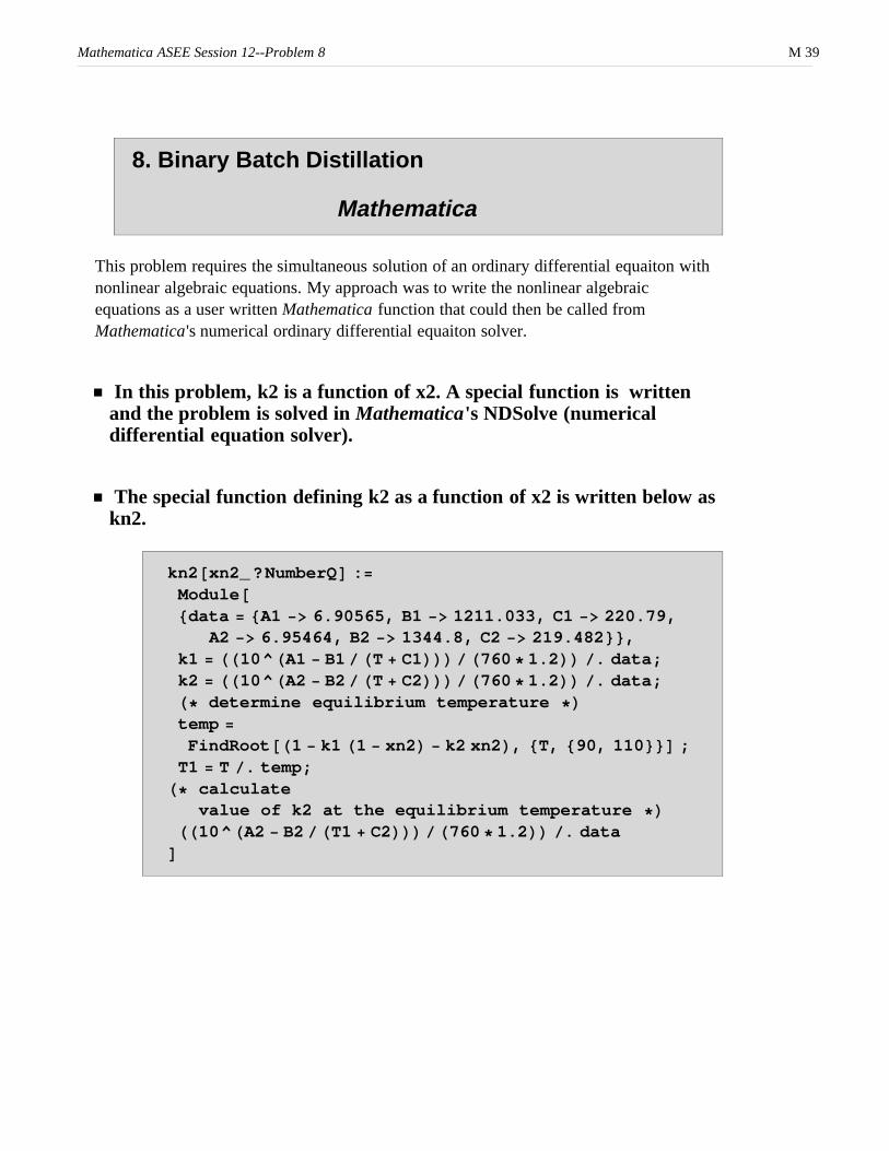
8. Binary Batch Distillation
Mathematica
This problem requires the simultaneous solution of an ordinary differential equaiton with nonlinear algebraic equations. My approach was to write the nonlinear algebraic equations as a user written Mathematica function that could then be called from Mathematica's numerical ordinary differential equaiton solver.
� In this problem, k2 is a function of x2. A special function is written and the problem is solved in Mathematica's NDSolve (numerical differential equation solver).
� The special function defining k2 as a function of x2 is written below as kn2.
kn2@xn2_?NumberQD :=Module@8data = 8A1 -> 6.90565, B1 -> 1211.033, C1 -> 220.79,
A2 -> 6.95464, B2 -> 1344.8, C2 -> 219.482<<,k1 = HH10^HA1 - B1 � HT + C1LLL � H760 * 1.2LL �. data;k2 = HH10^HA2 - B2 � HT + C2LLL � H760 * 1.2LL �. data;H* determine equilibrium temperature *Ltemp =FindRoot@H1 - k1 H1 - xn2L - k2 xn2L, 8T, 890, 110<<D ;T1 = T �. temp;
H* calculatevalue of k2 at the equilibrium temperature *L
HH10^HA2 - B2 �HT1 + C2LLL �H760 * 1.2LL �. dataD
Mathematica ASEE Session 12--Problem 8 M 39

� Once the special function is defined, the problem is solved using Mma's built-in numerical ODE solver, NDSolve .
eqn2 = eqn = L'@x2D == L@x2D� Hx2 Hkn2@x2D - 1LL
L¢@x2D ==L@x2D
������������������������������������������������x2 H-1 + kn2@x2DL
solution =NDSolve@8eqn2, [email protected] == 100<, L@x2D, 8x2, 0.4, 0.8<D
88L@x2D ® [email protected], 0.8<<, <>D@x2D<<
Plot@L@x2D �. solution, 8x2, 0.4, 0.8<,PlotRange -> 880.4, 0.8<, 80, 100<<D
0.45 0.5 0.55 0.6 0.65 0.7 0.75 0.8
20
40
60
80
100
� Graphics �
solution �. x2 -> 0.8 H* value of L at x2=0.8 *L
[email protected] ® 14.0417<<
T1 H* final temperature *L
108.572
Mathematica ASEE Session 12--Problem 8 M 40
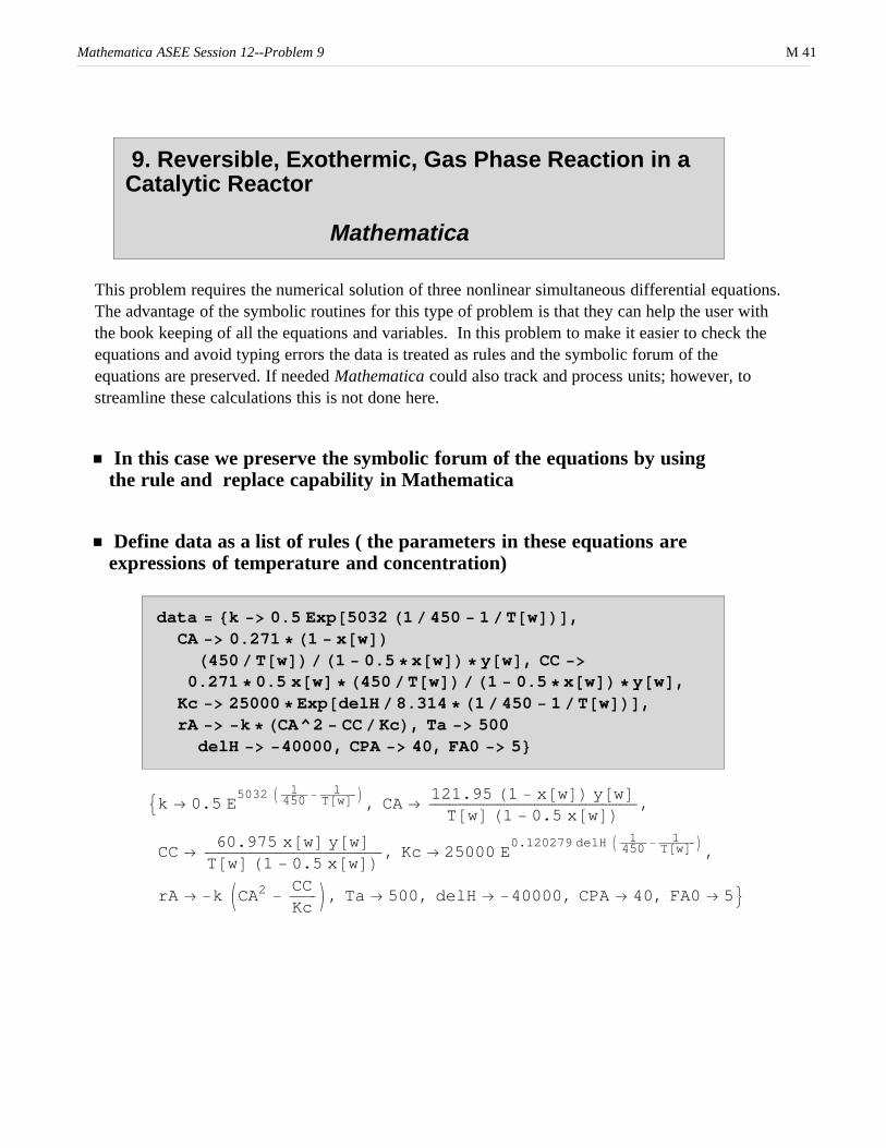
9. Reversible, Exothermic, Gas Phase Reaction in a Catalytic Reactor
Mathematica
This problem requires the numerical solution of three nonlinear simultaneous differential equations. The advantage of the symbolic routines for this type of problem is that they can help the user with the book keeping of all the equations and variables. In this problem to make it easier to check the equations and avoid typing errors the data is treated as rules and the symbolic forum of the equations are preserved. If needed Mathematica could also track and process units; however, to streamline these calculations this is not done here.
� In this case we preserve the symbolic forum of the equations by using the rule and replace capability in Mathematica
� Define data as a list of rules ( the parameters in these equations are expressions of temperature and concentration)
data = 8k -> 0.5 Exp@5032 H1 � 450 - 1 �T@wDLD,CA -> 0.271 * H1 - x@wDL
H450 � T@wDL� H1 - 0.5 *x@wDL* y@wD, CC ->0.271 * 0.5 x@wD* H450 �T@wDL� H1 - 0.5 *x@wDL *y@wD,Kc -> 25000 * Exp@delH � 8.314 * H1 � 450 - 1 �T@wDLD,rA -> -k * HCA^2 - CC � KcL, Ta -> 500
delH -> -40000, CPA -> 40, FA0 -> 5<
9k ® 0.5 E5032 I 1�����������450 - 1���������������T@wD M
, CA ®121.95 H1 - x@wDL y@wD�������������������������������������������������������������T@wD H1 - 0.5 x@wDL
,
CC ®60.975 x@wD y@wD
����������������������������������������������������T@wD H1 - 0.5 x@wDL
, Kc ® 25000 E0.120279 delH I 1�����������450 - 1���������������T@wD M
,
rA ® -k JCA2 -CC��������Kc
N, Ta ® 500, delH ® -40000, CPA ® 40, FA0 ® 5=
Mathematica ASEE Session 12--Problem 9 M 41

� Define differential equations . The three equations are assigned to the variable names eqn1, eqn2, and eqn3. This simplifies the users task of checking for typos and avoids re-typing.
eqn1 = x'@wD == -rA � FA0 ��. data;eqn2 = T'@wD ==
HH0.8 HTa - T@wDL + rA * delHL � HCPA *FA0LL ��. data;eqn3 = y'@wD ==
-0.015 * H1 - 0.5 x@wDL HT@wD� 450L �H2 *y@wDL ��.data;
� Check eqn1
eqn1 H* Check Equation 1 *L
x¢@wD ==
0.1 E5032 I 1�����������450 - 1���������������T@wD M
i
k
jjjjjj-0.002439 E
4811.16 I 1�����������450 - 1���������������T@wD Mx@wD y@wD
������������������������������������������������������������������������������������������������������T@wD H1 - 0.5 x@wDL
+
14871.8 H1 - x@wDL2 y@wD2����������������������������������������������������������������������
T@wD2 H1 - 0.5 x@wDL2
y
{
zzzzzz
Mathematica ASEE Session 12--Problem 9 M 42

� Solve the three ODE equations
H* Mathematica gives numerical solutionsto ODEs are interpolating polynomialsas shown below. This makes it easy inMathematica to view and use the solutions *L
solutions = NDSolve@8eqn1, x@0D == 0,eqn2, T@0D == 450, eqn3, y@0D == 1<, 8x@wD,
T@wD, y@wD<, 8w, 0, 20<D
88x@wD ® InterpolatingFunction@880., 20.<<, <>D@wD,T@wD ® InterpolatingFunction@880., 20.<<, <>D@wD,y@wD ® InterpolatingFunction@880., 20.<<, <>D@wD<<
Mathematica ASEE Session 12--Problem 9 M 43

� Plot the three solutions versus w
H* Plot of profiles for x, T, and y versus w *L
Plot@Evaluate@8x@wD, T@wD �1000, y@wD< �. solutionsD, 8w, 0, 20<,
PlotRange -> 880, 20<, 80, 1.5<<,PlotStyle -> [email protected],
[email protected]<, [email protected]<,[email protected], [email protected], 0.05<D<<D
H* x=dashed, T=black, y=gray *L
2.5 5 7.5 10 12.5 15 17.5 20
0.2
0.4
0.6
0.8
1
1.2
1.4
� Graphics �
Mathematica ASEE Session 12--Problem 9 M 44

à Part (b) The rapid increase is due to the exotermic reation quickly accelerating due to the increasing temperature even though the reatant concentration is falling. Equilibrium is rapidly achieved after this hot spot appears. The temperature and conversion reduce only slightly due to the external heat transfer which tends to slightly cool the reator as the reating mixture contiues toward the reactor exit.
à Part (c) Plot CA and CC from 0<w<20.
Plot@Evaluate@88CA, CC< �. data< �. solutionsD, 8w, 0, 20<,PlotRange -> 880, 20<, 80, 0.3<<,PlotStyle -> [email protected]<,[email protected], [email protected], 0.05<D<<D
H* CC=dashed, CA=solid black *L
2.5 5 7.5 10 12.5 15 17.5 20
0.05
0.1
0.15
0.2
0.25
0.3
� Graphics �
Mathematica ASEE Session 12--Problem 9 M 45

10. Dynamics of a Heated Tank with PI Temperature Control
Mathematica
This problem requires the solution of several simultaneous ordinary differential equaitons and the solution of a PI controller with step input. Problem 10 is the longest and most complicated of the set. Mathematica v3.0 gives the user the ability to use special symbols so one can match the actual mathematical equations. Symbol will match those of the problem statement.
à Part (a) Demonstrate the open loop system with Kc = 0. At t = 10 minutes the inlet temperature Ti is changed from 80 oC to 40 oC. The Pade approximation is not necessary in Mathematica since a delay function is easy to write directly and is 100% accurate. However the Pade function will also be demonstrated for completeness.
à Define parameters and other relations
data = 9WCp -> 500 H*flow rate x heat capacity *L,
rVCp -> 4000 H* denisty x volume x heat capacity *L,
td -> 1 H* dead time *L,tm -> 5 H* measured temperature *L,Tr -> 80 H* set point temperature *L,Kc -> 0 H* controller gain *L,tI -> 2 H* integral time *L,D -> If@t < 10, 0, 1D H* step function *L,Ti -> 60 + D H-20L H* inlet temperature *L,
q -> 10000 + Kc HTr - Tm@tDL +Kc��������tI
errsum@tD,
dTdt ->WCp HTi - T@tDL + q��������������������������������������������������
rVCp=;
Mathematica ASEE Session 12--Problem 10 M 46

data �� ColumnForm H* display the inputs *L
WCp ® 500
rVCp ® 4000
td ® 1
tm ® 5Tr ® 80
Kc ® 0
tI ® 2
D ® If@t < 10, 0, 1D
Ti ® 60 - 20 D
q ® 10000 + errsum@tD Kc����������������������������tI
+ Kc HTr - Tm@tDL
dTdt ®q+WCp HTi-T@tDL�����������������������������������
rVCp
à Define differential equations
eqn1 = T'@tD ==HWCp HTi - T@tDL + qL��������������������������������������������������������
rVCp��. data
eqn2 = To'@tD == JT@tD - To@tD - Jtd��������2
N dTdtN 2
��������td
��. data
eqn3 = Tm'@tD ==i
kjjHTo@tD - Tm@tDL��������������������������������������������
tm
y
{zz ��. data
eqn4 = errsum'@tD == Tr - Tm@tD ��. data
T¢@tD ==10000 + 500 H60 - 20 If@t < 10, 0, 1D - T@tDL����������������������������������������������������������������������������������������������������������������������
4000
To¢@tD == 2 J-10000 - 500 H60 - 20 If@t < 10, 0, 1D - T@tDL��������������������������������������������������������������������������������������������������������������������������
8000+
T@tD - To@tDN
Tm¢@tD ==1�����5
H-Tm@tD + To@tDL
errsum¢@tD == 80 - Tm@tD
Mathematica ASEE Session 12--Problem 10 M 47

� Solve the differential equations
solutions = NDSolve@8eqn1, T@0D == 80,eqn2, To@0D == 80,eqn3, Tm@0D == 80,eqn4, errsum@0D == 0<,8T@tD, To@tD, Tm@tD, errsum@tD<, 8t, 0, 60<D
88T@tD ® InterpolatingFunction@880., 60.<<, <>D@tD,To@tD ® InterpolatingFunction@880., 60.<<, <>D@tD,Tm@tD ® InterpolatingFunction@880., 60.<<, <>D@tD,errsum@tD ® InterpolatingFunction@880., 60.<<, <>D@tD<<
Plot@Evaluate@8T@tD, To@tD, Tm@tD< �. solutionsD, 8t, 0, 60<,
PlotRange -> 880, 60<, 860, 81<<,PlotStyle -> [email protected]<,
[email protected], [email protected]<,[email protected], [email protected], 0.05<D<<D
H* T is thin line, To is gray, andTm is dashed *L
10 20 30 40 50 60
65
70
75
80
� Graphics �
Mathematica ASEE Session 12--Problem 10 M 48
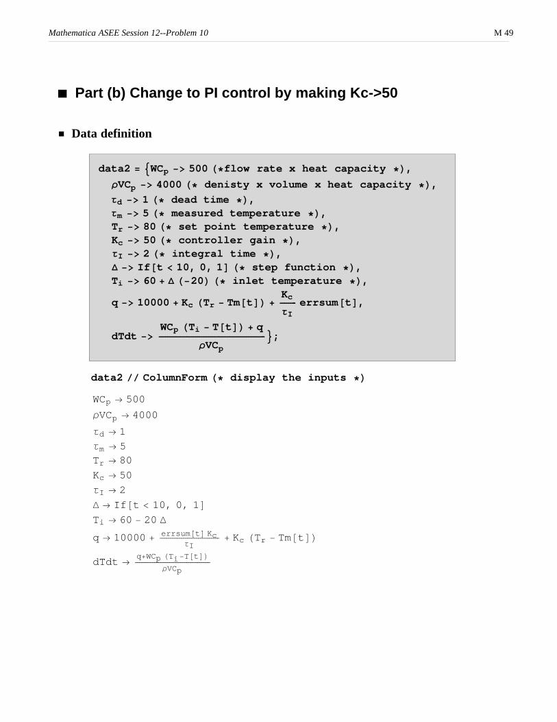
à Part (b) Change to PI control by making Kc->50
� Data definition
data2 = 9WCp -> 500 H*flow rate x heat capacity *L,
rVCp -> 4000 H* denisty x volume x heat capacity *L,
td -> 1 H* dead time *L,tm -> 5 H* measured temperature *L,Tr -> 80 H* set point temperature *L,Kc -> 50 H* controller gain *L,tI -> 2 H* integral time *L,D -> If@t < 10, 0, 1D H* step function *L,Ti -> 60 + D H-20L H* inlet temperature *L,
q -> 10000 + Kc HTr - Tm@tDL +Kc��������tI
errsum@tD,
dTdt ->WCp HTi - T@tDL + q��������������������������������������������������
rVCp=;
data2 �� ColumnForm H* display the inputs *L
WCp ® 500
rVCp ® 4000
td ® 1
tm ® 5Tr ® 80
Kc ® 50
tI ® 2
D ® If@t < 10, 0, 1D
Ti ® 60 - 20 D
q ® 10000 + errsum@tD Kc����������������������������tI
+ Kc HTr - Tm@tDL
dTdt ®q+WCp HTi-T@tDL�����������������������������������
rVCp
Mathematica ASEE Session 12--Problem 10 M 49

� Place data into equations
eqn1 = T'@tD ==HWCp HTi - T@tDL + qL��������������������������������������������������������
rVCp��. data2
eqn2 = To'@tD == JT@tD - To@tD - Jtd��������2
N dTdtN 2
��������td
��. data2
eqn3 = Tm'@tD ==i
kjjHTo@tD - Tm@tDL��������������������������������������������
tm
y
{zz ��. data2
eqn4 = errsum'@tD == Tr - Tm@tD ��. data2
T¢@tD ==1
��������������4000
H10000 + 25 errsum@tD +
500 H60 - 20 If@t < 10, 0, 1D - T@tDL + 50 H80 - Tm@tDLL
To¢@tD == 2 JT@tD +1
��������������8000
H-10000 - 25 errsum@tD - 500
H60 - 20 If@t < 10, 0, 1D - T@tDL - 50 H80 - Tm@tDLL -
To@tDN
Tm¢@tD ==1�����5
H-Tm@tD + To@tDL
errsum¢@tD == 80 - Tm@tD
� Solve equations
solutions2 = NDSolve@8eqn1, T@0D == 80, eqn2,To@0D == 80, eqn3, Tm@0D == 80, eqn4, errsum@0D == 0<,
8T@tD, To@tD, Tm@tD, errsum@tD<, 8t, 0, 200<D
88T@tD ® InterpolatingFunction@880., 200.<<, <>D@tD,To@tD ® InterpolatingFunction@880., 200.<<, <>D@tD,Tm@tD ® InterpolatingFunction@880., 200.<<, <>D@tD,errsum@tD ®InterpolatingFunction@880., 200.<<, <>D@tD<<
Mathematica ASEE Session 12--Problem 10 M 50

� Plot results
Plot@Evaluate@8T@tD, To@tD, Tm@tD< �. solutions2D, 8t, 0, 200<,
PlotRange -> 880, 200<, 860, 85<<,PlotStyle -> [email protected]<,
[email protected], [email protected]<,[email protected], [email protected], 0.05<D<<D
H* T is black line, To is gray, and Tm is dashed *L
25 50 75 100 125 150 175 200
65
70
75
80
85
� Graphics �
Mathematica ASEE Session 12--Problem 10 M 51

à Part (c) Change to PI control by making Kc->500
� Data definition
data3 = 9WCp -> 500 H*flow rate x heat capacity *L,
rVCp -> 4000 H* denisty x volume x heat capacity *L,
td -> 1 H* dead time *L,tm -> 5 H* measured temperature *L,Tr -> 80 H* set point temperature *L,Kc -> 500 H* controller gain *L,tI -> 2 H* integral time *L,D -> If@t < 10, 0, 1D H* step function *L,Ti -> 60 + D H-20L H* inlet temperature *L,
q -> 10000 + Kc HTr - Tm@tDL +Kc��������tI
errsum@tD,
dTdt ->WCp HTi - T@tDL + q��������������������������������������������������
rVCp=;
data3 �� ColumnForm H* display the inputs *L
WCp ® 500
rVCp ® 4000
td ® 1
tm ® 5Tr ® 80
Kc ® 500
tI ® 2
D ® If@t < 10, 0, 1D
Ti ® 60 - 20 D
q ® 10000 + errsum@tD Kc����������������������������tI
+ Kc HTr - Tm@tDL
dTdt ®q+WCp HTi-T@tDL�����������������������������������
rVCp
Mathematica ASEE Session 12--Problem 10 M 52

� Place data into equations
eqn1 = T'@tD ==HWCp HTi - T@tDL + qL��������������������������������������������������������
rVCp��. data3
eqn2 = To'@tD == JT@tD - To@tD - Jtd��������2
N dTdtN 2
��������td
��. data3
eqn3 = Tm'@tD ==i
kjjHTo@tD - Tm@tDL��������������������������������������������
tm
y
{zz ��. data3
eqn4 = errsum'@tD == Tr - Tm@tD ��. data3
T¢@tD ==1
��������������4000
H10000 + 250 errsum@tD +
500 H60 - 20 If@t < 10, 0, 1D - T@tDL + 500 H80 - Tm@tDLL
To¢@tD == 2 JT@tD +1
��������������8000
H-10000 - 250 errsum@tD - 500
H60 - 20 If@t < 10, 0, 1D - T@tDL - 500 H80 - Tm@tDLL -
To@tDN
Tm¢@tD ==1�����5
H-Tm@tD + To@tDL
errsum¢@tD == 80 - Tm@tD
solutions3 = NDSolve@8eqn1, T@0D == 80, eqn2,To@0D == 80, eqn3, Tm@0D == 80, eqn4, errsum@0D == 0<,
8T@tD, To@tD, Tm@tD, errsum@tD<, 8t, 0, 200<D
88T@tD ® InterpolatingFunction@880., 200.<<, <>D@tD,To@tD ® InterpolatingFunction@880., 200.<<, <>D@tD,Tm@tD ® InterpolatingFunction@880., 200.<<, <>D@tD,errsum@tD ®InterpolatingFunction@880., 200.<<, <>D@tD<<
Mathematica ASEE Session 12--Problem 10 M 53

� Plot results
Plot@Evaluate@8T@tD, To@tD, Tm@tD< �. solutions3D, 8t, 0, 200<,
PlotRange -> 880, 200<, 860, 100<<,PlotStyle -> [email protected]<,
[email protected], [email protected]<,[email protected], [email protected], 0.05<D<<D
H* T is black line, To is gray, and Tm is dashed *L
25 50 75 100 125 150 175 200
65
70
75
80
85
90
95
100
� Graphics �
Mathematica ASEE Session 12--Problem 10 M 54

à Part (d) Closed loop with proportional control only
� Data definition
data4 = 9WCp -> 500 H*flow rate x heat capacity *L,
rVCp -> 4000 H* denisty x volume x heat capacity *L,
td -> 1 H* dead time *L,tm -> 5 H* measured temperature *L,Tr -> 80 H* set point temperature *L,Kc -> 500 H* controller gain *L,tI -> 2 H* integral time *L,D -> If@t < 10, 0, 1D H* step function *L,Ti -> 60 + D H-20L H* inlet temperature *L,
q -> 10000 + Kc HTr - Tm@tDL, dTdt ->WCp HTi - T@tDL + q��������������������������������������������������
rVCp=;
data4 �� ColumnForm H* display the inputs *L
WCp ® 500
rVCp ® 4000
td ® 1
tm ® 5Tr ® 80
Kc ® 500
tI ® 2
D ® If@t < 10, 0, 1D
Ti ® 60 - 20 D
q ® 10000 + Kc HTr - Tm@tDL
dTdt ®q+WCp HTi-T@tDL�����������������������������������
rVCp
Mathematica ASEE Session 12--Problem 10 M 55

� Place data into equations
eqn1 = T'@tD ==HWCp HTi - T@tDL + qL��������������������������������������������������������
rVCp��. data4
eqn2 = To'@tD == JT@tD - To@tD - Jtd��������2
N dTdtN 2
��������td
��. data4
eqn3 = Tm'@tD ==i
kjjHTo@tD - Tm@tDL��������������������������������������������
tm
y
{zz ��. data4
eqn4 = errsum'@tD == Tr - Tm@tD ��. data4
T¢@tD ==1
��������������4000
H10000 + 500 H60 - 20 If@t < 10, 0, 1D - T@tDL +
500 H80 - Tm@tDLL
To¢@tD == 2 JT@tD +1
��������������8000
H-10000 - 500
H60 - 20 If@t < 10, 0, 1D - T@tDL - 500 H80 - Tm@tDLL -
To@tDN
Tm¢@tD ==1�����5
H-Tm@tD + To@tDL
errsum¢@tD == 80 - Tm@tD
� Solve equations
solutions4 = NDSolve@8eqn1, T@0D == 80, eqn2,To@0D == 80, eqn3, Tm@0D == 80, eqn4, errsum@0D == 0<,
8T@tD, To@tD, Tm@tD, errsum@tD<, 8t, 0, 60<D
88T@tD ® InterpolatingFunction@880., 60.<<, <>D@tD,To@tD ® InterpolatingFunction@880., 60.<<, <>D@tD,Tm@tD ® InterpolatingFunction@880., 60.<<, <>D@tD,errsum@tD ® InterpolatingFunction@880., 60.<<, <>D@tD<<
Mathematica ASEE Session 12--Problem 10 M 56

� Plot results
Plot@Evaluate@8T@tD, To@tD, Tm@tD< �. solutions4D, 8t, 0, 60<,
PlotRange -> 880, 60<, 865, 82<<,PlotStyle -> [email protected]<,
[email protected], [email protected]<,[email protected], [email protected], 0.05<D<<D
H* T is black line, To is gray, and Tm is dashed *L
� Graphics �
à Part (e) Closed loop with peformance limits on q
� Data definition
data5 = 9WCp -> 500 H*flow rate x heat capacity *L,
rVCp -> 4000 H* denisty x volume x heat capacity *L,
td -> 1 H* dead time *L,tm -> 5 H* measured temperature *L,Tr -> 80 + D * 10H* set point temperature *L,Kc -> 5000 H* controller gain *L,tI -> 2 H* integral time *L,D -> If@t < 10, 0, 1D H* step function *L,Ti -> 60H* inlet temperature *L,q -> 10000 + Kc HTr - Tm@tDL,qlim -> If@q < 0, 0, If@q >= 2.6 * 10000, 2.6 * 10000, qDDH* calculate the limits on q *L,
dTdt ->WCp HTi - T@tDL + qlim�����������������������������������������������������������
rVCp=;
Mathematica ASEE Session 12--Problem 10 M 57

data5 �� ColumnForm H* display the inputs *L
WCp ® 500
rVCp ® 4000
td ® 1
tm ® 5Tr ® 80 + 10 D
Kc ® 5000
tI ® 2
D ® If@t < 10, 0, 1D
Ti ® 60
q ® 10000 + Kc HTr - Tm@tDL
qlim ® If@q < 0, 0, If@q ³ 2.6 10000, 2.6 10000, qDD
dTdt ®qlim+WCp HTi-T@tDL������������������������������������������
rVCp
data4 = 8WC -> 500, rhoVCp -> 4000, taud -> 1, taum -> 5,Tr -> 80 + step * 10, Kc -> 5000, step -> If@t < 10, 0, 1D,Ti -> 60, q -> 10000 + Kc HTr - Tm@tDL, qlim ->If@q < 0, 0, If@q >= 2.6 * 10000, 2.6 *10000, qDD,dTdt -> HWC HTi - T@tDL + qlimL� rhoVCp<
9WC ® 500, rhoVCp ® 4000,
taud ® 1, taum ® 5, Tr ® 80 + 10 step, Kc ® 5000,step ® If@t < 10, 0, 1D, Ti ® 60, q ® 10000 + Kc HTr - Tm@tDL,qlim ® If@q < 0, 0, If@q ³ 2.6 10000, 2.6 10000, qDD,
dTdt ®qlim + WC HTi - T@tDL���������������������������������������������������������
rhoVCp=
Mathematica ASEE Session 12--Problem 10 M 58

� Place data into equations
eqn1 = T'@tD ==HWCp HTi - T@tDL + qlimL�����������������������������������������������������������������
rVCp��. data5
eqn2 = To'@tD == JT@tD - To@tD - Jtd��������2
N dTdtN 2
��������td
��. data5
eqn3 = Tm'@tD == i
kjjHTo@tD - Tm@tDL��������������������������������������������
tm
y
{zz ��. data5
eqn4 = errsum'@tD == Tr - Tm@tD ��. data5
T¢@tD ==1
��������������4000
HIf@10000 + 5000 H80 + 10 If@t < 10, 0, 1D - Tm@tDL < 0,
0, If@10000 + 5000 HH80 + 10 If@t < 10, 0, 1DL - Tm@tDL ³2.6 10000, 2.6 10000,
10000 + 5000 HH80 + 10 If@t < 10, 0, 1DL - Tm@tDLDD +500 H60 - T@tDLL
To¢@tD == 2 J1
��������������8000
H-If@10000 +
5000 H80 + 10 If@t < 10, 0, 1D - Tm@tDL < 0, 0, If@10000 + 5000 HH80 + 10 If@t < 10, 0, 1DL - Tm@tDL ³2.6 10000,
2.6 10000, 10000 +5000 HH80 + 10 If@t < 10, 0, 1DL - Tm@tDLDD -
500 H60 - T@tDLL +
T@tD - To@tDN
Tm¢@tD ==1�����5
H-Tm@tD + To@tDL
errsum¢@tD == 80 + 10 If@t < 10, 0, 1D - Tm@tD
Mathematica ASEE Session 12--Problem 10 M 59

� Solve equations
solutions5 = NDSolve@8eqn1, T@0D == 80, eqn2,To@0D == 80, eqn3, Tm@0D == 80, eqn4, errsum@0D == 0<,
8T@tD, To@tD, Tm@tD, errsum@tD<, 8t, 0, 200<D
88T@tD ® InterpolatingFunction@880., 200.<<, <>D@tD,To@tD ® InterpolatingFunction@880., 200.<<, <>D@tD,Tm@tD ® InterpolatingFunction@880., 200.<<, <>D@tD,errsum@tD ®InterpolatingFunction@880., 200.<<, <>D@tD<<
� Plot results
Plot@Evaluate@8T@tD, To@tD, Tm@tD< �. solutions5D, 8t, 0, 200<,
PlotRange -> 880, 200<, 870, 100<<,PlotStyle -> [email protected]<,
[email protected], [email protected]<,[email protected], [email protected], 0.05<D<<D
H* T is black line, To is gray, and Tm is dashed *L
25 50 75 100 125 150 175 200
75
80
85
90
95
100
� Graphics �
Mathematica ASEE Session 12--Problem 10 M 60

à Generate the plot of q and qlim versus time.Define the q and qlim time dependent functions.
temp1 = H10000 + Kc HTr - Tm@tDL ��. data5L �. solutions5
810000 + 5000 H80 + 10 If@t < 10, 0, 1D -InterpolatingFunction@880., 200.<<, <>D@tDL<
qfun@t_D := temp1 H* q time dependent function *L
temp2 = HIf@q < 0, 0,If@q >= 2.6 * 10000, 2.6 *10000, qDD ��. data5L �.
solutions5
8If@10000 + 5000 H80 + 10 If@t < 10, 0, 1D -InterpolatingFunction@880., 200.<<, <>D@tDL < 0,
0,If@10000 + 5000 HH80 + 10 If@t < 10, 0, 1DL -
InterpolatingFunction@880., 200.<<, <>D@tDL ³2.6 10000, 2.6 10000,
10000 + 5000 HH80 + 10 If@t < 10, 0, 1DL -InterpolatingFunction@880., 200.<<, <>D@tDLDD<
qlimfun@t_D := temp2 H* qlim time dependent function *L
H* Note that the plot is scaled bydividing both "q " and "qlim
" by 104 *L
Mathematica ASEE Session 12--Problem 10 M 61

Plot@8qfun@tD �10^4, qlimfun@tD �10^4<,8t, 0, 200<, PlotPoints ® 25,PlotRange -> 880, 200<, 8-1, 7<<,PlotStyle -> [email protected]<,
[email protected], [email protected]<<D
H* Black line is "q " and gray line is "qlim " *L
25 50 75 100 125 150 175 200
-1
1
2
3
4
5
6
7
� Graphics �
Mathematica ASEE Session 12--Problem 10 M 62


![Chemical Engineering Course Curriculum for the New ...Chemical Engineering courses CL152: Introduction to Chemical Engineering, [2 1 0 6] Historical overview of Chemical Engineering:](https://static.fdocuments.in/doc/165x107/5e962b5aae543b3a820d5617/chemical-engineering-course-curriculum-for-the-new-chemical-engineering-courses.jpg)


