Generating and using truly random quantum states in

Mathematica

Jaros law Adam MiszczakInstitute of Theoretical and Applied Informatics,

Polish Academy of Sciences, Ba ltycka 5, 44-100 Gliwice, Poland

30/07/2011 (v. 0.23)

Abstract

The problem of generating random quantum states is of a great interest from the quantum in-formation theory point of view. In this paper we present a package for Mathematica computingsystem harnessing a specific piece of hardware, namely Quantis quantum random number generator(QRNG), for investigating statistical properties of quantum states. The described package imple-ments a number of functions for generating random states, which use Quantis QRNG as a sourceof randomness. It also provides procedures which can be used in simulations not related directly toquantum information processing.Keywords: random density matrices ; quantum information ; quantum random number generatorsPACS numbers: 03.67.-a ; 02.70.Wz ; 07.05.Tp

Program Summary

Program title: TRQSProgram author: Jaros law A. MiszczakDistribution format: tar.gzNo. of bytes in distributed program, including test data, etc.: 8.9 · 104

No. of lines in distributed program, including test data, etc.: ∼ 1000Programming language: Mathematica, CComputer: any supporting the recent version of MathematicaOperating system: any platform supporting Mathematica; tested with GNU/Linux (32 and 64 bit)RAM: case-dependentNature of problem: Generation of random density matrices.Method of solution: Use of a physical quantum random number generator.

1 Introduction

As full scale quantum computing devices are still missing, the simulation of quantum computers hasgained considerable attention as a method for investigation the behaviour of quantum algorithms andprotocols [1]. It also provides a valuable method for inspecting the mathematical structure of quantumtheory by providing information about statistical properties of quantum states and operations [2].

Generating random numbers using the statistical nature of quantum theory provides one of the firstpractical applications of quantum information theory. At the same time the high quality of randomnumbers generated using quantum random number generators is based on the very basic principles ofNature [3]. Since random numbers are important in many areas of human activity, at the moment thisprovides one of the most important applications of quantum information theory.

During the last several years many simulators of quantum computers have been developed and themost up-to-date list of available software is available at [1]. Many simulators of quantum informationprocessing were developed using Mathematica computing system [4, 5, 6, 7, 8]. Also some attention hasbeen devoted to utilising CUDA programming model [9] and parallel processing model [10, 11, 12]. The

1

arX

iv:1

102.

4598

v2 [

quan

t-ph

] 1

9 O

ct 2

011

research effort in using parallel and distributed computing for the purpose of quantum information pro-cessing was motivated by the amount of computational resources needed in order to perform a simulationof quantum computation.

In this paper we present a TRQS (True Quantum Random States) package for Mathematica comput-ing system harnessing a specific piece of hardware, namely Quantis quantum random number generator(QRNG), for investigating statistical properties of quantum states. The described package implementsa number of functions for using numbers and generating random states (i.e. random state vectors andrandom density matrices), using Quantis QRNG as the source of randomness. The presented packagehas been developed for the purpose of quantum information theory, but it can be easily utilised in otherareas of science.

The motivation for utilising random numbers generated using quantum devices is twofold. Firstly,QRNGs provide a high-quality source of randomness which can be used in various areas of computationalphysics. Recent progress in this area [13] suggests that QRNGs are of a great interest for experimentalists,as well as theorists, working in the field of quantum information theory. Secondly, it has been shownthat the statistical properties of obtained numbers cannot be reproduced using standard methods ofgenerating random numbers [3].

This paper is organised as follows. In Section 2 we introduce basic theoretical facts concerning randomstates and operations. In Section 3 we describe the functions implemented in the presented package andin Section 4 we use the described package to analyse some problems related to quantum informationtheory. We also use TRQS package be benchmark the speed of Quantis random number generator.Finally, in Section 5, we provide some concluding remarks and discuss the alternative sources of randomnumbers generated using quantum random number generators.

2 Random quantum states

The problem of generating random quantum states is of a great interest from the quantum informationtheory point of view. Random states appear naturally in many situations in quantum informationprocessing, especially when one must deal with the unavoidable interaction of the system in questionwith the environment.

We start by recalling some basic facts used in the rest of this paper. For a more complete introductionto mathematical concepts used in quantum information theory see e.g. [14, 2]. Next, we present theselected methods of generating random density matrices implemented in the TRQS package. Moredetailed description of the methods for generating random quantum density matrices can be foundin [15].

2.1 Basic definitions

In what follows we restrict our attention to finite-dimensional spaces. We denote by |φ〉 ∈ Cn pure statesi.e. normalised elements of the vector space Cn. By Mm,n we denote the set of all m× n matrices overC and the set of square n × n matrices is denoted by Mn. The set of n-dimensional density matrices(normalised, positive semi-definite operators on Cn) is denoted by Ωn. The set Mn has the structureof a Hilbert space with the scalar product given by (A,B) = trA†B. This particular Hilbert space isknown as the Hilbert-Schmidt space of operators acting on Cn and we will denote it by HHS.

In particular, Ωn ⊂ Mn. Moreover, any element of Ωn can be represented as a convex combination(mixture) of one-dimensional projectors. For any ρ ∈ Ωn there exists a sequence of non-negative numbersp1, p2, . . . , pn such that ρ =

∑ni=1 piPi, where Pi, i = 1, 2, . . . , n is a sequence of orthonormal one-

dimensional projectors. Extreme elements of the set Ωn are exactly the pure states and can be identifiedwith ket vectors |ψ〉 ' |ψ〉〈ψ|. Convex combinations of pure states are refereed to as mixed states.

2.2 Random pure states

In most cases to describe quantum algorithms and protocols one assumes that it is possible to avoidunnecessary interactions with the environment [2]. In such situation the state of the system remainspure during the evolution, which is represented by a unitary matrix.

2

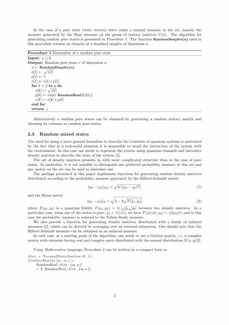
In the case of a pure state (state vectors) there exists a natural measure in the set, namely themeasure generated by the Haar measure on the group of unitary matrices U(n). The algorithm forgenerating random pure states is presented in Procedure 1. The function RandomSimplex(n) used inthis procedure returns an element of a standard simplex of dimension n.

Procedure 1 Generation of a random pure state

Input: n ≥ 0Output: Random pure state v of dimension ns← RandomSimplex(n)

a[1]←√s[1]

p[1]← 1v[1]← a[1] ∗ p[1]for k = 2 to n doa[k]←

√s[i]

p[k]← exp(i RandomReal(0,2π))v[k]← a[k] ∗ p[k]

end forreturn v

Alternatively a random pure states can be obtained by generating a random unitary matrix andchoosing its columns as random pure states.

2.3 Random mixed states

The need for using a more general formalism to describe the evolution of quantum systems is motivatedby the fact that in a real-world situation it is impossible to avoid the interaction of the system withthe environment. In this case one needs to represent the system using quantum channels and introducedensity matrices to describe the state of the system [2].

The set of density matrices presents us with more complicated structure than in the case of purestates. In particular, it is not possible to distinguish one preferred probability measure in this set andany metric on the set can be used to introduce one.

The package presented in this paper implements functions for generating random density matricesdistributed according to the probability measure generated by the Hilbert-Schmidt metric

‖ρ1 − ρ2‖HS =√

tr [(ρ1 − ρ2)2], (1)

and the Bures metric

‖ρ1 − ρ2‖B =

√2− 2

√F (ρ1, ρ2) (2)

where F (ρ1, ρ2) is a quantum fidelity F (ρ1, ρ2) = tr |√ρ1√ρ2| between two density matrices. In a

particular case, when one of the states is pure, ρ1 = |ψ〉〈ψ|, we have F (|φ〉〈φ|, ρ2) = 〈φ|ρ2|ψ〉 and in thiscase the probability measure is reduced to the Fubini-Study measure.

We also provide a function for generating density matrices distributed with a family of inducedmeasures [2], which can be derived by averaging over an external subsystem. One should note that theHilbert-Schmidt measure can be obtained as an induced measure.

In each case, as a starting point of the algorithm, one needs to use a Ginibre matrix, i.e. a complexmatrix with elements having real and complex parts distributed with the normal distribution N (x, y)[2].

Using Mathematica language, Procedure 2 can be written in a compact form as

d i s t = NormalDistr ibut ion [ 0 , 1 ] ;GinibreMatr ix [ m , n ] :=

RandomReal [ d i s t ,m, n ]+ I RandomReal [ d i s t ,m, n ]

3

Procedure 2 Generation of the random matrix from the Ginibre ensemble.Input: m,n > 0Output: Matrix G of size m× n

for k = 1 to m dofor l = 1 to n doG[k, l]← RandomReal(0,1) + i RandomReal(0,1)

end forend forreturn G

2.3.1 Induced measures and the Hilbert-Schmidt ensemble

The Hilbert-Schmidt metric defined in Eq. 1 is commonly used to describe the metric structure of theset of quantum states. This distance introduces a Euclidean geometry in the space of density matrices.In the special case of one-qubit density matrices, the space has the form of the Bloch ball.

The Hilbert-Schmidt measure belongs to the class of induced measures [2, Ch.14]. In a general case,one can seek a source of randomness in a given system, by studying the interaction of the n-dimensionalsystem in question with the environment. In such situation the random states to model the behaviour ofthe system should be generated by reducing a pure state in N ×K-dimensional space. In what followswe denote the resulting probability measure by µN,K .

In particular, the Hilbert-Schmidt probability measure on n-dimensional space Ωn can be obtainedby reducing a bi-partite pure quantum state from CN×N . However, it is easy to see that this measure,as well as any measure µN,K , can be obtained by using a simpler procedure.

We start by observing that any complex matrix X ∈ M(C) can be used to construct a normalised,

positive matrix XX†

trXX† . Let us now assume that we have a pure state in the N × K-dimensionalHilbert space, |ψ〉 ∈ HN ⊗ HK = CN×K . Any such state can be represented in a product basis

|ψ〉 =∑Ni=1

∑Kj=1Xij |i〉 ⊗ |j〉, where X ∈ MN,K . The matrix XX† is, in this case, equivalent to

the partial trace of |ψ〉〈ψ| with respect to the second subsystem, trHK|ψ〉〈ψ| = XX†. Symmetrically we

have trHN|ψ〉〈ψ| = X†X.

It follows from the above considerations that the spectrum of a density matrix obtained using thismethod is the set of squared and normalised singular values of the matrix X. In particular, if one assumesthat the pure states on HK ⊗HN are distributed according to the Fubini-Study measure, the resultingdensity matrices are distributed with induced measures.

In the case of induced measures the elements of the coefficient matrix are independent randomvariables and form a Ginibre matrix.

Procedure 3 Generation of a random density matrix distributed according to induced probabilitymeasure µn,k obtained by tracing out the ancillary system of dimension k.

Input: n ≥ 0, k ≥ 2Output: Random mixed state ρ of dimension nG← GinibreMatrix(n,k)

ρ← GG†

ρ← 1tr ρρ

return ρ

In the special case of K = N we obtain the Hilbert-Schmidt ensemble.The statistical properties of the set of quantum states with respect to the probability measure intro-

duced by the Hilbert-Schmidt metric were studied in [16, 17].

2.3.2 Bures ensemble

Another popular measure of the distance between quantum states is the Bures distance. Its usage ismotivated by the fact that this distance, when restricted to diagonal matrices, is equivalent to theHellinger distance in statistics, defined for two discrete probability distributions as H(p,q) =

∑i

√piqi.

4

Moreover, the Bures distance and quantum fidelity are related to the distinguishability of quantum states,defined as a trace distance between the given states.

The above features distinguish the Bures measure as an optimal method for generating randomdensity matrices in the situation when no information about the source of state is present.

The algorithm for generating random density matrices distributed according to the probability mea-sure based on the Bures distance was provided in [18]. This algorithm is presented in Procedure 4.

Procedure 4 Generation of a random density matrix distributed according to the probability measureinduced by the Bures metric

Input: n ≥ 0Output: Random mixed state ρ of dimension nG← GinibreMatrix(n,n)

U ← RandomUnitary(n)

ρ← (1 + U)GG†(1 + U†)ρ← 1

tr ρρreturn ρ

3 Description of the package

The TRQS package implements a number of functions allowing to obtain random state vectors andrandom density matrices.

It uses Quantis random number generator produced by ID Quantique [19] for the purpose of generatingrandom numbers. ID Quantique provides drivers, example programs and a library for accessing Quantisdevices on most popular operating systems. The software package for using Quantis, including someexamples of how libQuantis library can be used, can be downloaded from the ID Quantique supportpage [20].

Note that the functions implemented are independent from the actual source of randomness. Inparticular it is possible to switch to some other sources of random numbers.

The package consists of a set of source files, developed using MathLink provided by Mathematica anda package file TRQS.m, implementing the main functionality.

3.1 Communication with Quantis device

In the presented package the communication between Mathematica and Quantis device was implementedusing MathLink – a standard interface for interprogramme communication provided by Mathematica.

We used libQuantis library that provides a number of functions for reading random data fromQuantis device. In particular the presented package uses only functions for reading basic data types.The functions of this kind implemented in libQuantis can be divided into four categories

• QuantisReadShort and QuantisReadScaledShort – functions for reading short integers and shortintegers within the given range,

• QuantisReadInt and QuantisReadScaledInt – functions for reading long integers and long inte-gers within the given range,

• QuantisReadFloat 01 and QuantisReadScaledFloat functions for reading float numbers in therange [0, 1] and float numbers within the given range,

• QuantisReadDouble 01 and QuantisReadScaledDouble – functions for reading double numbersin the range [0, 1] and double numbers within the given range.

Moreover, the library function QuantisRead allows to read raw random data. This function can bealso used to read large amount of data, which can be necessary in the case when one needs to fill largematrices with random numbers.

5

3.2 Organisation of the package

The described package was designed to work in companion with the QI package for Mathematica [7]and can be used along with this package. The provided functions for generating random states can begrouped into three categories: basic functions, functions for generating pure states and unitary matricesand functions for generating mixed states and channels.

The functions are defined within the TRQS name space. We follow the naming convention whichassumes that functions using a true random number generator to produce results have names starting withTrue and the rest of the name describes the generated object. The functions related to the configurationof the back-end i.e. Quantis device, have names starting with Quantis (see: Sec. 3.2.4).

Each function is provided along with some basic information about its functionality.

3.2.1 Basic functions

The first group of functions implements basic structures utilised for generating quantum states. Thefunctions in this group implement communication with Quantis device and provide the generation ofreal and integer random numbers and some basic structures. In this group the following functions allowto access basic types of random numbers:

1. TrueRandomReal – returns a random real (double) number; this function is based on libQuantis

library function QuantumReadScaledDouble and is implemented in three variants:

(a) TrueRandomReal[nmin, nmax] – returns a real number distributed uniformly in the interval[nmin, nmax],

(b) TrueRandomReal[nmax] – returns a real number distributed uniformly in the interval [0, nmax],

(c) TrueRandomReal[] – returns a real number distributed uniformly in the interval [0, 1],

2. TrueRandomRealNormal[x,y,d1, . . . , dl] – returns a (d1× . . .× dl)-dimensional array of randomnumbers distributed according to N (x, y).

3. TrueRandomInteger – returns a random integer. This function, based on libQuantis libraryfunction QuantumReadScaledInt, is provided for convenience and implemented in three variants:

(a) TrueRandomInteger[nmin, nmax] – returns an integer distributed uniformly in the interval[nmin, nmax],

(b) TrueRandomInteger[nmax] – returns an integer distributed uniformly in the interval [0, nmax],

(c) TrueRandomInteger[] – returns 0 or 1.

The following functions, built using these basic functions, allow to obtain the structures used to constructrandom quantum states and operations:

1. TrueRandomSimplex[n] – returns an element of a standard simplex, distributed uniformly onsimplex,

2. TrueGinibreMatrix[m,n] – returns an n×m Ginibre matrix,

3. TrueRandomChoice[e1,e2,...,en] – returns at random one of the e1,e2,. . . ,en.,

4. TrueRandomGraph[v,e, form] – returns a pseudorandom graph with v vertices and e edges. Ad-ditionally, the last argument can be set to ”Graph” (default) to obtain a graphical representationof the result or to ”List” to obtain the result as a list of vertices and edges.

3.2.2 Pure states and unitary matrices

The functions in this group allow to obtain random pure states and random unitary matrices. Sinceproduct (or local) states and operations are of a special interest in quantum information theory, weprovide functions allowing to generate pure states and unitary matrices of the tensor product structure

1. TrueRandomKet[n] – returns a random pure state in n-dimensional space Cn,

6

2. TrueRandomProductKet[n1, n2, ...nk] – returns a random pure state, which is an element ofspace with the tensor product structure Cn1 ⊗ Cn2 ⊗ . . .⊗ Cnk

3. TrueRandomUnitary[n] – returns a random unitary matrix acting on n-dimensional space Cn,

4. TrueRandomLocalUnitary[n1, n2, ...nk] – returns a random unitary matrix, which acts on theelements of space with the tensor product structure Cn1 ⊗ Cn2 ⊗ . . .⊗ Cnk

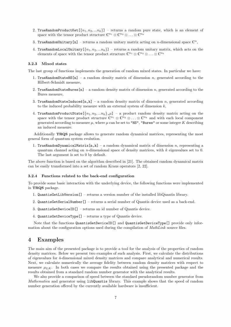
3.2.3 Mixed states

The last group of functions implements the generation of random mixed states. In particular we have:

1. TrueRandomStateHS[n] – a random density matrix of dimension n, generated according to theHilbert-Schmidt measure,

2. TrueRandomStateBures[n] – a random density matrix of dimension n, generated according to theBures measure,

3. TrueRandomStateInduced[n,k] – a random density matrix of dimension n, generated accordingto the induced probability measure with an external system of dimension k,

4. TrueRandomProductState[n1, n2, ...nk,µ] – a product random density matrix acting on thespace with the tensor product structure Cn1 ⊗ Cn2 ⊗ . . . ⊗ Cnk and with each local componentgenerated according to measure µ, where µ can be set to "HS", "Bures" or some integerK describingan induced measure.

Additionally TRQS package allows to generate random dynamical matrices, representing the mostgeneral form of quantum system evolution.

1. TrueRandomDynamicalMatrix[n,k] – a random dynamical matrix of dimension n, representing aquantum channel acting on n-dimensional space of density matrices, with k eigenvalues set to 0.The last argument is set to 0 by default.

The above function is based on the algorithm described in [21]. The obtained random dynamical matrixcan be easily transformed into a set of random Kraus operators [2, 22].

3.2.4 Functions related to the back-end configuration

To provide some basic interaction with the underlying device, the following functions were implementedin TRQS package.

1. QuantisGetLibVersion[] – returns a version number of the installed libQuantis library.

2. QuantisGetSerialNumber[] – returns a serial number of Quantis device used as a back-end.

3. QuantisGetDeviceID[] – returns an id number of Quantis device.

4. QuantisGetDeviceType[] – returns a type of Quantis device.

Note that the functions QuantisGetDeviceID[] and QuantisGetDeviceType[] provide only infor-mation about the configuration options used during the compilation of MathLink source files.

4 Examples

The main aim of the presented package is to provide a tool for the analysis of the properties of randomdensity matrices. Below we present two examples of such analysis. First, we calculate the distributionsof eigenvalues for 4-dimensional mixed density matrices and compare analytical and numerical results.Next, we calculate numerically the average fidelity between random density matrices with respect tomeasure µ2,K . In both cases we compare the results obtained using the presented package and theresults obtained from a standard random number generator with the analytical results.

We also provide a comparison of speed between the standard pseudorandom number generator fromMathematica and generator using libQuantis library. This example shows that the speed of randomnumber generation offered by the currently available hardware is insufficient.

7

4.1 Distribution of eigenvalues

The Bures and Hilbert-Schmidt probability measures are of the product form i.e. the distribution ofeigenvalues is independent from the distribution of eigenvectors.

In the case of the Hilbert-Schmidt measure the probability density of eigenvalues is given by theformula [2]

PHS(λ1, . . . , λN ) = CHSN

∏i<j

(λi − λj)2, (3)

where∑i λi = 1, λi ≤ 0, i = 1, 2, . . . , N . The normalisation constant CHS

N reads

CHSN =

Γ(N2)∏Ni=1 Γ(k)Γ(k + 1)

. (4)

0.0 0.2 0.4 0.6 0.8 1.0Λ

10

20

30

40

50

60PHΛL

Λ1

Λ2

Λ3 Λ4

(a) Analytical results obtained by a direct integrationover appropriate subsets of the convex hull of the spec-trum.

0.0 0.2 0.4 0.6 0.8 1.0Λ0

10

20

30

40

50

60PHΛL

(b) Numerical results obtained using random states gen-erated with TRQS package.

Figure 1: Distribution of eigenvalues for random density matrices distributed uniformly according to theHilbert-Schmidt probability measure.

Here we present some results for the Hilbert-Schmidt measure and density matrices of dimension 4.The distribution of eigenvalues λ1, λ2, λ3, λ4 of the random density matrices from Ω4 generated uniformlywith respect to the Hilbert-Schmidt measure is presented in Fig. 1(a). In Fig. 1(b) the distribution ofλ1, λ2, λ3, λ4 obtained using true random density matrices is presented. Numerical results were obtainedusing a sample of 2000 random density matrices.

4.2 Average fidelity

Quantum fidelity [2] is commonly used in quantum information theory to quantify to what degree a givenquantum state can be approximated by some other state or a family of states [23].

The average fidelity between two random quantum states can be used e.g. to provide an insightinto the performance of quantum protocols in the presence of noise. Since, in most cases, in quantuminformation processing one is interested in the behaviour of 2-dimensional systems (qubits), below wedeal with this case only.

As it has already been mentioned, the use of random states in quantum information processing iscommonly motivated by the interaction of the system in question with the environment. In this caseone is interested in random density matrices generated uniformly with respect to some induced measureµ2,K , where K is the dimension of the ancillary system.

The mean fidelity between two one-qubit random density matrices generated uniformly with respectto measure µN,K was calculated in [17] and reads

〈F 〉2,K =1

2+

1

2

(Γ(K − 1

2

)Γ(K + 1

2

)Γ(K − 1)Γ(K + 1)

)2

. (5)

8

2 4 6 8 10 12 14 16K0.6

0.7

0.8

0.9

1.0XF\

Figure 2: Average fidelity between one-qubit random mixed states generated uniformly with respectto µ2,K . The dotted line represents the exact result. Numerical results obtained using the presentedpackage are marked with ”×”.

The average fidelity for one-qubit random states generated with µ2,K is presented in Fig. 2. Theresults were obtained using a sample of 50 states and one can see that in this case it allows to obtain avery good approximation of an exact result, especially in the case of large K.

4.3 Speed comparison

For the purpose of testing the speed of the TRQS package we have performed three experiments involvinggeneration of random real numbers distributed uniformly on the unit interval. In each experiment wehave used a different method.

æ

æ

æ

æ

æ

æ

æ

à

à

à

à

à

à

à

ì

ì

ì

ì

ì

ì

ì

1 2 3 4 5 6 7

- 5

- 4

- 3

- 2

-1

0

1

2

3

4

5

sample size

timein

sec

Figure 3: Comparison of speed for random number generators in log-log scale. Blue circles representtimings for samples generated using RandomReal[] functions using pseudo-random number generator.Red squares represent timings for samples generated with TRQS package function TrueRandomReal[]

using MathLink executables linked against libQuantis-NoHW library. Black diamonds illustrate timingsfor an analogous method with MathLink executables linked against libQuantis library.

1. The first experiment was conducted using a standard pseudo-random number generator providedby Mathematica. Additionally we used ClearSystemCache[’’Numeric’’] in order to generate theresults independent from previous computations.

2. In the second experiment the numbers were generated using TRQS package and MathLink exe-cutables linked against libQuantis-NoHW library. While in this case the generated numbers are

9

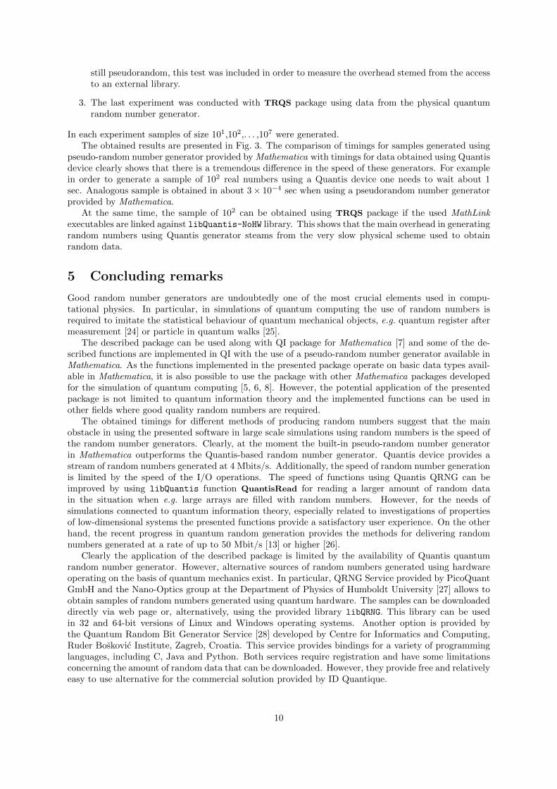
still pseudorandom, this test was included in order to measure the overhead stemed from the accessto an external library.

3. The last experiment was conducted with TRQS package using data from the physical quantumrandom number generator.

In each experiment samples of size 101,102,. . . ,107 were generated.The obtained results are presented in Fig. 3. The comparison of timings for samples generated using

pseudo-random number generator provided by Mathematica with timings for data obtained using Quantisdevice clearly shows that there is a tremendous difference in the speed of these generators. For examplein order to generate a sample of 102 real numbers using a Quantis device one needs to wait about 1sec. Analogous sample is obtained in about 3× 10−4 sec when using a pseudorandom number generatorprovided by Mathematica.

At the same time, the sample of 102 can be obtained using TRQS package if the used MathLinkexecutables are linked against libQuantis-NoHW library. This shows that the main overhead in generatingrandom numbers using Quantis generator steams from the very slow physical scheme used to obtainrandom data.

5 Concluding remarks

Good random number generators are undoubtedly one of the most crucial elements used in compu-tational physics. In particular, in simulations of quantum computing the use of random numbers isrequired to imitate the statistical behaviour of quantum mechanical objects, e.g. quantum register aftermeasurement [24] or particle in quantum walks [25].

The described package can be used along with QI package for Mathematica [7] and some of the de-scribed functions are implemented in QI with the use of a pseudo-random number generator available inMathematica. As the functions implemented in the presented package operate on basic data types avail-able in Mathematica, it is also possible to use the package with other Mathematica packages developedfor the simulation of quantum computing [5, 6, 8]. However, the potential application of the presentedpackage is not limited to quantum information theory and the implemented functions can be used inother fields where good quality random numbers are required.

The obtained timings for different methods of producing random numbers suggest that the mainobstacle in using the presented software in large scale simulations using random numbers is the speed ofthe random number generators. Clearly, at the moment the built-in pseudo-random number generatorin Mathematica outperforms the Quantis-based random number generator. Quantis device provides astream of random numbers generated at 4 Mbits/s. Additionally, the speed of random number generationis limited by the speed of the I/O operations. The speed of functions using Quantis QRNG can beimproved by using libQuantis function QuantisRead for reading a larger amount of random datain the situation when e.g. large arrays are filled with random numbers. However, for the needs ofsimulations connected to quantum information theory, especially related to investigations of propertiesof low-dimensional systems the presented functions provide a satisfactory user experience. On the otherhand, the recent progress in quantum random generation provides the methods for delivering randomnumbers generated at a rate of up to 50 Mbit/s [13] or higher [26].

Clearly the application of the described package is limited by the availability of Quantis quantumrandom number generator. However, alternative sources of random numbers generated using hardwareoperating on the basis of quantum mechanics exist. In particular, QRNG Service provided by PicoQuantGmbH and the Nano-Optics group at the Department of Physics of Humboldt University [27] allows toobtain samples of random numbers generated using quantum hardware. The samples can be downloadeddirectly via web page or, alternatively, using the provided library libQRNG. This library can be usedin 32 and 64-bit versions of Linux and Windows operating systems. Another option is provided bythe Quantum Random Bit Generator Service [28] developed by Centre for Informatics and Computing,Ruder Boskovic Institute, Zagreb, Croatia. This service provides bindings for a variety of programminglanguages, including C, Java and Python. Both services require registration and have some limitationsconcerning the amount of random data that can be downloaded. However, they provide free and relativelyeasy to use alternative for the commercial solution provided by ID Quantique.

10

6 Acknowledgements

Author would like to acknowledge interesting discussions with K. Zyczkowski and W. Roga and somestimulating programming exercises conducted with Z. Pucha la and P. Gawron. Thanks also goes toL. Widmer for motivating this work and H. Weier for his comments concerning the recent progress inthe area of quantum random generation methods. Author would like to thank the anonymous reviewerfor his motivating comments concerning the development of the package.

This work was supported by the Polish National Science Centre under the grant number N N516475440 and by the Polish Ministry of Science and Higher Education under the grants number N N519442339 and IP 2010 052 270.

References

[1] Quantiki. List of QC simulators. http://www.quantiki.org/wiki/List_of_QC_simulators.

[2] I. Bengtsson and K. Zyczkowski. Geometry of Quantum States. Cambridge University Press, Cam-bridge, UK, 2006.

[3] C.S. Calude, M.J. Dinneen, M. Dumitrescu, and K. Svozil. Experimental evidence of quantumrandomness incomputability. Phys. Rev. A, 82(2):022102, 2010.

[4] H. Touchette and P. Dumais. The quantum computation package for Mathematica 4.0. http:

//crypto.cs.mcgill.ca/QuCalc/.

[5] B. Julia-Dıaz, J.M. Burdis, and F. Tabakin. QDENSITY—a Mathematica quantum computersimulation. Comp. Phys. Comm., 174:914–934, 2006. http://www.pitt.edu/~tabakin/QDENSITY/QDENSITY.htm.

[6] J. L. Gomez-Munoz and F. Delgado-Cepeda. Quantum 2.0 for Mathematica 7. http://homepage.cem.itesm.mx/lgomez/quantum/.

[7] J. A. Miszczak, Z. Pucha la, and P. Gawron. QI package for Mathematica, 2010. Software freelyavailable at http://zksi.iitis.pl/wiki/projects:mathematica-qi.

[8] B. Julia-Dıaz and F. Tabakin. QCWAVE, a mathematica quantum computer simulation update.http://www.pitt.edu/~tabakin/QW/.

[9] E. Gutierrez, S. Romero, M.A. Trenas, and E.L. Zapata. Quantum computer simulation using thecuda programming model. Comp. Phys. Comm., 181(2):283 – 300, 2010.

[10] I. Glendinning and B. Omer. Parallelization of the QC-lib quantum computer simulator library. InR. Wyrzykowski and et al., editors, 5th International Conference on Parallel Processing and AppliedMathematics, volume 3019 of LNCS, pages 461–468, 2004.

[11] K. De Raedt, K. Michielsen, H. De Raedt, B. Trieu, G. Arnold, M. Richter, Th. Lippert, H. Watan-abe, and N. Ito. Massively parallel quantum computer simulator. Comp. Phys. Comm., 176(2):121– 136, 2007.

[12] F. Tabakin and B. Julia-Dıaz. QCMPI: A parallel environment for quantum computing. Comp.Phys. Comm., 180(6):948 – 964, 2009.

[13] M. Furst, H. Weier, S. Nauerth, D.G. Marangon, Ch. Kurtsiefer, and H. Weinfurter. High speedoptical quantum random number generation. Optics Express, 18(12):13029–13037, 2010.

[14] T. Heinosaari and M. Ziman. Guide to mathematical concepts of quantum theory. Acta Phys.Slovaca, 58(4):487–674, 2008.

[15] K. Zyczkowski, K. A. Penson, I. Nechita, and B. Collins. Generating random density matrices. J.Math. Phys., 52:062201, 2011.

11

[16] K. Zyczkowski and H.-J. Sommers. Hilbert-Schmidt volume of the set of mixed quantum states. J.Phys. A-Math. Theor., 36(39):10115, 2003.

[17] K. Zyczkowski and H.-J. Sommers. Average fidelity between random quantum states. Phys. Rev.A, 71(3):032313, 2005.

[18] V. Al Osipov, H.-J. Sommers, and K. Zyczkowski. Random Bures mixed states and the distributionof their purity. J. Phys. A: Math. Theor., 43:055302, 2010.

[19] ID Quantique SA. http://www.idquantique.com/.

[20] Quantis support page. http://www.idquantique.com/support/quantis-trng.html.

[21] W. Bruzda, V. Cappellini, H.-J. Sommers, and K. Zyczkowski. Random quantum operations. Phys.Lett. A, 373(3):320, 2009.

[22] J.A. Miszczak. Singular value decomposition and matrix reorderings in quantum information theory.Int. J. Mod. Phys. C, 2011. in press.

[23] D. Markham, J. A. Miszczak, Z. Pucha la, and K. Zyczkowski. Quantum state discrimination: Ageometric approach. Phys. Rev. A, 77:042111, 2008.

[24] B. Omer. Quantum programming in QCL. Master’s thesis, Vienna University of Technology, 2000.

[25] F. L. Marquezino and R. Portugal. The QWalk simulator of quantum walks. Comp. Phys. Comm.,179(5):359–369, 2008.

[26] T. Symul, S.M. Assad, and P.K. Lam. Real time demonstration of high bitrate quantum randomnumber generation with coherent laser light. Appl. Phys. Lett., 98(23):231103, 2011.

[27] QRNG Service. Project developed by PicoQuant GmbH and the Nano-Optics groups at the De-partment of Physics of Humboldt University, https://qrng.physik.hu-berlin.de/.

[28] Quantum Random Bit Generator Service. Project developed by Centre for Informatics and Com-puting, Ruder Boskovic Institute, Zagreb, Croatia, http://random.irb.hr/.

12