MATH6038 | Mathematics for Science 2.2 with Maple · PDF file29/02/2012 · In the...
55
MATH6038 — Mathematics for Science 2.2 with Maple J.P. McCarthy February 29, 2012
Transcript of MATH6038 | Mathematics for Science 2.2 with Maple · PDF file29/02/2012 · In the...

MATH6038 — Mathematics for Science 2.2 with Maple
J.P. McCarthy
February 29, 2012

Contents
0.1 Introduction . . . . . . . . . . . . . . . . . . . . . . . . . . . . . . . . . . . . 20.2 Motivation: Network Flows & How to Make a Decision. . . . . . . . . . . . . 5
1 Matrix Algebra 81.1 Systems of Linear Equations . . . . . . . . . . . . . . . . . . . . . . . . . . . 81.2 Row Operations and Gaussian Elimination . . . . . . . . . . . . . . . . . . . 111.3 Matrices . . . . . . . . . . . . . . . . . . . . . . . . . . . . . . . . . . . . . . 221.4 Matrix Inverses . . . . . . . . . . . . . . . . . . . . . . . . . . . . . . . . . . 301.5 Determinants . . . . . . . . . . . . . . . . . . . . . . . . . . . . . . . . . . . 31
2 Statistics 322.1 Data Analysis . . . . . . . . . . . . . . . . . . . . . . . . . . . . . . . . . . . 322.2 Data Presentation . . . . . . . . . . . . . . . . . . . . . . . . . . . . . . . . . 35
3 Probability 433.1 Introduction . . . . . . . . . . . . . . . . . . . . . . . . . . . . . . . . . . . . 433.2 Random Variables . . . . . . . . . . . . . . . . . . . . . . . . . . . . . . . . . 433.3 Independence . . . . . . . . . . . . . . . . . . . . . . . . . . . . . . . . . . . 433.4 Conditional Probability . . . . . . . . . . . . . . . . . . . . . . . . . . . . . . 443.5 Tree & Reliability Block Diagrams . . . . . . . . . . . . . . . . . . . . . . . 443.6 Binomial Distribution . . . . . . . . . . . . . . . . . . . . . . . . . . . . . . . 453.7 Poisson Distribution . . . . . . . . . . . . . . . . . . . . . . . . . . . . . . . 463.8 Normal Distribution . . . . . . . . . . . . . . . . . . . . . . . . . . . . . . . 463.9 Sampling . . . . . . . . . . . . . . . . . . . . . . . . . . . . . . . . . . . . . . 493.10 Quality Control Charts . . . . . . . . . . . . . . . . . . . . . . . . . . . . . . 513.11 Bayesian Statistics . . . . . . . . . . . . . . . . . . . . . . . . . . . . . . . . 52
1

MATH6038 — Mathematics for Science 2.2 with Maple 2
0.1 Introduction
Lecturer
J.P. McCarthy
Office
Meetings before class by appointment via email only.
Email & Web:
[email protected] and http://irishjip.wordpress.comThis page will comprise the webpage for this module and as such shall be the venue forcourse announcements including a definitive date for the test. This page shall also housesuch resources as links (such as to exam papers), as well supplementary material. Please notethat not all items here are relevant to MATH6038; only those in the category ‘MATH6038’.Feel free to use the comment function therein as a point of contact.
Module Objective
This modules involves the study of matrices, statistics and probability distributions.
Module Content
Matrix Algebra
Matrix operations, properties of matrix operations, determinants, properties of determinants,row operations, Gaussian elimination, inverse matrices, solving linear system of equations,investigation of the solution space of linear system of equations.
Probability and Statistics
Presentation and analysis of data. Measures of central tendency; mean, mode and median.Measures of dispersion; range variance and standard deviation. Sample space, compoundevents, conditional probability, independent events, reliability block diagrams,Bayes Rule.Random variables, binomial, Poisson and Normal distributions. Introduction to sampling,confidence intervals for large and small samples. Construct and interpret quality controlcharts.
Assessment
Total Marks 100: End of Year Written Examination 70 marks; Continuous Assessment 30marks.
Continuous Assessment
The Continuous Assessment will be divided between a one hour written exam in Week 7worth 20% and your weekly participation in the Maple Lab (worth 10%).
MATH6038 — Mathematics for Science 2.2 with Maple 3
Absence from a test will not be considered accept in truly extraordinary cases. Plenty ofnotice will be given of the test date. For example, routine medical and dental appointmentswill not be considered an adequate excuse for missing the test.
Lectures
It will be vital to attend all lectures as many of the examples, proofs, etc. will be completedby us in class.
Maple Labs
Maple Labs will commence next week and are designed to explore and reinforce mathematicalconcepts.
Exercises
There are many ways to learn maths. Two methods which aren’t going to work are
1. reading your notes and hoping it will all sink in
2. learning off a few key examples, solutions, etc.
By far and away the best way to learn maths is by doing exercises, and there are two mainreasons for this. The best way to learn a mathematical fact/ theorem/ etc. is by using it inan exercise. Also the doing of maths is a skill as much as anything and requires practise.I will present ye with a set of exercises every week. In this module the “Lecture-SupervisedLearning” is comprised of you doing these exercises, giving them to me on a weekly basis,me marking them, and returning them. In addition I will provide a set of solutions online.Everyone shall have access to the solution sets however.The webpage may contain a link to a set of additional exercises. Past exam papers are fairgame. Also during lectures there will be some things that will be left as an exercise. Howmuch time you can or should devote to doing exercises is a matter of personal taste but becertain that effort is rewarded in maths.
Reading
Your primary study material shall be the material presented in the lectures; i.e. the lecturenotes. Exercises done in tutorials may comprise further worked examples. While the lectureswill present everything you need to know about MATH6038, they will not detail all there isto know. Further references are to be found in the library. Good references include:
• J. Bird, 2006, Higher Engineering Mathematics, Fifth Ed., Newnes.
• A. Croft & R. Davison, 2004, Mathematics for Engineers — A Modern InteractiveApproach, Pearson & Prentice Hall,
The webpage may contain supplementary material, and contains links and pieces abouttopics that are at or beyond the scope of the course. Finally the internet provides yetanother resource. Even Wikipedia isn’t too bad for this area of mathematics! You areencouraged to exploit these resources; they will also be useful for further maths modules.

MATH6038 — Mathematics for Science 2.2 with Maple 4
Exam
The exam format will roughly follow last year’s. Acceding to the maxim that learning off afew key examples, solutions, etc. is bad and doing exercises is good, solutions to past papersshall not be made available (by me at least). Only by trying to do the exam papers yourselfcan you guarantee proficiency. If you are still stuck at this stage feel free to ask the questioncome tutorial time.

MATH6038 — Mathematics for Science 2.2 with Maple 5
0.2 Motivation: Network Flows & How to Make a De-
cision.
Coughs seem very common here, especially among the children, though people lookstrong and healthy, but in the absence of proper statistics one cannot undertaketo say whether the district is a healthy one or not.
Edward Burnett Tylor
Network Flows
Suppose we have a network of one-way streets as shown in the diagram:
Figure 1: The flow of cars into junction A is 500 cars per hour, and 400 and 100 cars perhour emerge from B and C. Suppose the flows along the streets are f1, . . . , f6 cars per hour.From the simple rule that the flow into a junction must equal to flow out, how much can wetell about the internal workings of the network?
Equating the flow in with the flow out at each junction we get:
Junction A 500 = f1 + f2 + f3Junction B f1 + f4 + f6 = 400Junction C f3 + f5 = f6 + 100Junction D f2 = f4 + f5
.
This gives four equations in six variables f1, . . . , f6:
f1 + f2 + f3 = 500
f1 + f4 + f6 = 400
f3 + f5 − f6 = 100
f2 − f4 − f5 = 0
In the first section of the module we will learn how to solve these types of equations. Wewill find out if there are many solutions, a unique solution, or indeed no solution at all.
MATH6038 — Mathematics for Science 2.2 with Maple 6
How to Make a Decision.
Suppose that you are the ‘supervisor’ in a large factory with a production line. Whenattendance is low, the production line system doesn’t work as well, there are issues withhealth and safety and efficiency is reduced. There is going to be more than just a productionline in the factory; there will be a cleaning section, an admin section, a loading section, etc.;and if attendance is particularly low it might be prudent to call off production and insteadreallocate these workers to assist in these other departments.
Now there is a balance to achieve — we can’t afford to have the production line closed veryoften and neither do we want the production line to operating at a ‘half-assed’ capacity.Suppose the order come in from the main office that on 10% of the days, the productionline is to be closed down, and the workers reallocated to other tasks. The decision we needto make is; what days should we close the production line? We want to close on days whenattendance is low. We make assumptions such that we are not in Ireland so everyone isn’tcalling in sick on a Monday...
The answer is that we use statistics to do it. Essentially statistics is the science of data sothe very first thing we need to do is get data on absenteeism from the HR department. Fromthis data we will calculate the average attendance and the standard deviation. The standarddeviation is a measure of, on average, how spread out the data is, are there large deviationsfrom the average, or small deviations? Now a central plank of statistics theory: for manytypes of numerical data, there is an average which is also the outcome that occurred mostoften, and we are just as likely to be larger than the average as smaller than the average.When the number of employees is large, the attendance is like this. On most days there isa middling number of people in, some days a lot of people are absent, and on some daysnearly everyone is in.
MATH6038 — Mathematics for Science 2.2 with Maple 7
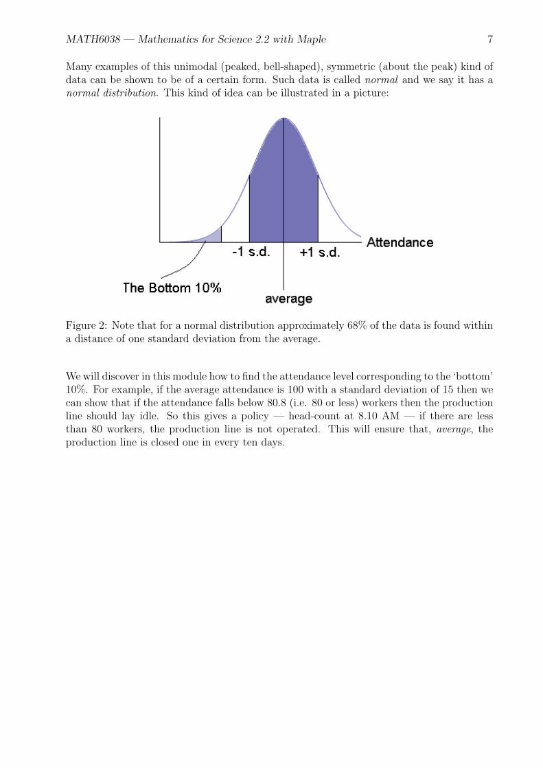
Many examples of this unimodal (peaked, bell-shaped), symmetric (about the peak) kind ofdata can be shown to be of a certain form. Such data is called normal and we say it has anormal distribution. This kind of idea can be illustrated in a picture:
Figure 2: Note that for a normal distribution approximately 68% of the data is found withina distance of one standard deviation from the average.
We will discover in this module how to find the attendance level corresponding to the ‘bottom’10%. For example, if the average attendance is 100 with a standard deviation of 15 then wecan show that if the attendance falls below 80.8 (i.e. 80 or less) workers then the productionline should lay idle. So this gives a policy — head-count at 8.10 AM — if there are lessthan 80 workers, the production line is not operated. This will ensure that, average, theproduction line is closed one in every ten days.

Chapter 1
Matrix Algebra
It is my experience that proofs involving matrices can be shortened by 50% if onethrows the matrices out.
Emil Artin.
In this chapter we learn how to solve and analyse equations such as the those generated bythe network flow question. Such a set of equations is known as a system of linear equations.For now a matrix is just a rectangular array of numbers in a bracket but later we will seetheir true nature.
1.1 Systems of Linear Equations
If two lines intersect they will do so at a single point; if two planes intersect their intersectionwill be a line, a line can intersect a plane at one point, lie in the plane, or not intersect itat all. Three planes can have one point in common or no points in common. Some of thesepossibilities are illustrated as follows:
Figure 1.1: Three planes can intersect at a point, a line, or nowhere.
We can show that the equation of a plane is given by:
What the hell is the equation of a plane? In essence it is a membership card:
8

MATH6038 — Mathematics for Science 2.2 with Maple 9
Hence to find the intersection of three planes we find points that are on all three curves —that is the satisfy their equations, at the same time, simultaneously. For example, we mighthave to find the points (x, y, z) that satisfy all of
3x+ 4y − z = 7
2x− 6y + z = −2
x− y + z = 3
1.1.1 Definitions
A linear equation in n variables is an equation of the form:
a1x1 + a2x2 + a3x3 + · · ·+ anxn = b, (1.1)
where the variables are x1, x2, . . . , xn, the numbers a1, . . . , an are called the coefficients, andb is the constant. A system of m equations in n variables has the form
a11x1 + a12x2 + · · ·+ a1nxn = b1
a21x1 + a22x2 + · · ·+ a2nxn = b2......
...
am1x1 + am2x2 + · · ·+ amnxn = bm.
Examples
Solve the following simultaneous equations.
1.
2x− y = 1
3x− 4y = 9
Solution 1 : This is the method taught in secondary schools. We will develop ourmethod along similar lines. Multiply the top equation by -4 and add the equationstogether:
Now back-substitute to get into either equation to get y = 1.Solution 2: This method is better for more general simultaneous equations (e.g. withx2 and the like). Solve the first equation for y = h(x):
MATH6038 — Mathematics for Science 2.2 with Maple 10
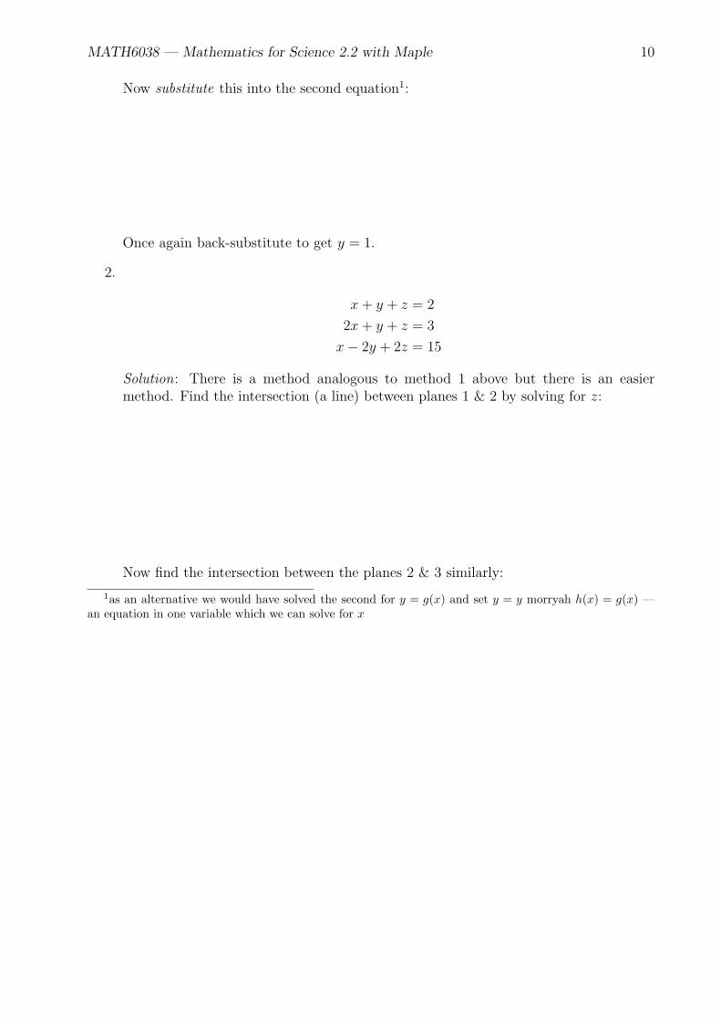
Now substitute this into the second equation1:
Once again back-substitute to get y = 1.
2.
x+ y + z = 2
2x+ y + z = 3
x− 2y + 2z = 15
Solution: There is a method analogous to method 1 above but there is an easiermethod. Find the intersection (a line) between planes 1 & 2 by solving for z:
Now find the intersection between the planes 2 & 3 similarly:
1as an alternative we would have solved the second for y = g(x) and set y = y morryah h(x) = g(x) —an equation in one variable which we can solve for x
MATH6038 — Mathematics for Science 2.2 with Maple 11
No just back-substitute to find z = −1. Solution: x = 1, y = 2, z = −1.
1.2 Row Operations and Gaussian Elimination
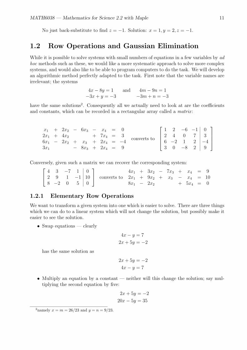
While it is possible to solve systems with small numbers of equations in a few variables by adhoc methods such as these, we would like a more systematic approach to solve more complexsystems, and would also like to be able to program computers to do the task. We will developan algorithmic method perfectly adapted to the task. First note that the variable names areirrelevant; the systems
4x− 8y = 1 and 4m− 9n = 1−3x+ y = −3 −3m+ n = −3
have the same solutions2. Consequently all we actually need to look at are the coefficientsand constants, which can be recorded in a rectangular array called a matrix :
x1 + 2x2 − 6x3 − x4 = 02x1 + 4x2 + 7x4 = 36x1 − 2x2 + x3 + 2x4 = −43x1 − 8x3 + 2x4 = 9
converts to
1 2 −6 −1 02 4 0 7 36 −2 1 2 −43 0 −8 2 9
Conversely, given such a matrix we can recover the corresponding system: 4 3 −7 1 0
2 9 1 −1 108 −2 0 5 0
converts to4x1 + 3x2 − 7x3 + x4 = 92x1 + 9x2 + x3 − x4 = 108x1 − 2x2 + 5x4 = 0
1.2.1 Elementary Row Operations
We want to transform a given system into one which is easier to solve. There are three thingswhich we can do to a linear system which will not change the solution, but possibly make iteasier to see the solution.
• Swap equations — clearly
4x− y = 7
2x+ 5y = −2
has the same solution as
2x+ 5y = −2
4x− y = 7
• Multiply an equation by a constant — neither will this change the solution; say mul-tiplying the second equation by five:
2x+ 5y = −2
20x− 5y = 35
2namely x = m = 26/23 and y = n = 9/23.

MATH6038 — Mathematics for Science 2.2 with Maple 12
• Add the equations together — why would this not change the solution?
2x+ 5y = 1
(20x− 5y) + (2x+ 5y) = 35− 2
Now we would have3 22x = 33 ⇒ x = 3/2. Note also that we could have put theselast two transformations into the single add a multiple of an equation to another.
If we go back into the augmented matrix picture we see:[4 −1 72 5 −2
]r1↔r2→
[2 5 −24 −1 7
]r2→r2×5→
[2 5 −220 −5 35
]r2→r2+r1→
[2 5 −222 0 33
],
and we can convert this into
2x+ 5y = −2
22x = 33
Note the row operations we enacted. Suppose we have a system of linear equations inaugmented matrix form [A|B]. From the discussions above we can show that the followingrow operations will leave the solution unchanged:
• swapping any two rows:
• multiplying any row by a constant:
• adding any row to any other:
• combining the last two: adding a multiple of a row to another row:
We call these the elementary row operations or EROs.
Example
Use the techniques above to simplify and hence solve the following simultaneous equation:
5x+ 7y = 0
−3x+ 4y = 2
Solution: First we write everything in augmented matrix form:
3[Ex]: from this find y

MATH6038 — Mathematics for Science 2.2 with Maple 13
What I am going to do is try to use the EROs to get the augmented matrix in the form
Hence we now have
Using the three EROs we want to take the augmented matrix form of the linear system andapply the EROs until the coefficient matrix is in row-echelon form. This looks like
MATH6038 — Mathematics for Science 2.2 with Maple 14
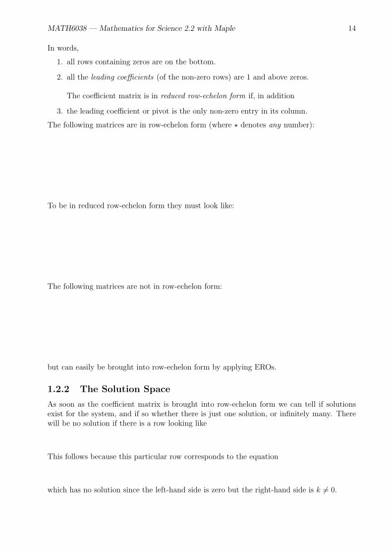
In words,
1. all rows containing zeros are on the bottom.
2. all the leading coefficients (of the non-zero rows) are 1 and above zeros.
The coefficient matrix is in reduced row-echelon form if, in addition
3. the leading coefficient or pivot is the only non-zero entry in its column.
The following matrices are in row-echelon form (where ⋆ denotes any number):
To be in reduced row-echelon form they must look like:
The following matrices are not in row-echelon form:
but can easily be brought into row-echelon form by applying EROs.
1.2.2 The Solution Space
As soon as the coefficient matrix is brought into row-echelon form we can tell if solutionsexist for the system, and if so whether there is just one solution, or infinitely many. Therewill be no solution if there is a row looking like
This follows because this particular row corresponds to the equation
which has no solution since the left-hand side is zero but the right-hand side is k = 0.

MATH6038 — Mathematics for Science 2.2 with Maple 15
If no such row appears then there is at least one solution. It is unique if every columncontains a pivot; if this is not so then the variables corresponding to the columns withoutpivots are not determined and become parameters/free variables in the solution leading toinfinitely many solutions.
Examples
The augmented matric for the three linear systems has been brought into reduced row-echelonform. Find the solutions:
(i)
1 0 0 −10 1 0 00 0 1 2
, (ii)
1 3 0 1 30 0 1 7 10 0 0 0 2
, (iii)
1 5 0 0 −2 30 0 1 0 4 −50 0 0 1 2 60 0 0 0 0 0
.
Solution:
(i) We simply have
(ii) Note the third row...
(iii) Rewrite this set of equations:
x1 + 5x2 − 2x5 = 3
x3 + 4x4 = 5
x4 + 2x5 = 6
0x5 = 0
No solve from the bottom. Firstly x5 could be anything. We write this by sayingx5 = t for t ∈ R. This means that x5 can take on any real number (R) value. In thiscase, x5 or t is called a parameter or free variable. For each value of the parameter(t), we get a different solution. As t can take on any value from minus to plus infinity,there are thus an infinite number of solutions. Now we look at the second last row:
Now at the third last:
Now look at the first equation:
Now for any fixed value of t, x1 = −5x1 + (3 + 2t) actually represents a line andthus there are an infinite number of pairs (x1, x2) that satisfy this equation. We needanother parameter/free variable. In this we could choose x1 or x2 but usually we will
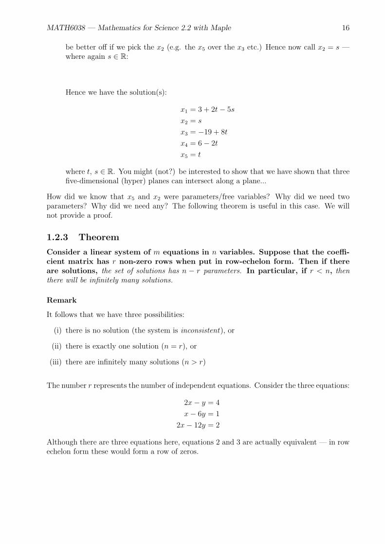
MATH6038 — Mathematics for Science 2.2 with Maple 16
be better off if we pick the x2 (e.g. the x5 over the x3 etc.) Hence now call x2 = s —where again s ∈ R:
Hence we have the solution(s):
x1 = 3 + 2t− 5s
x2 = s
x3 = −19 + 8t
x4 = 6− 2t
x5 = t
where t, s ∈ R. You might (not?) be interested to show that we have shown that threefive-dimensional (hyper) planes can intersect along a plane...
How did we know that x5 and x2 were parameters/free variables? Why did we need twoparameters? Why did we need any? The following theorem is useful in this case. We willnot provide a proof.
1.2.3 Theorem
Consider a linear system of m equations in n variables. Suppose that the coeffi-cient matrix has r non-zero rows when put in row-echelon form. Then if thereare solutions, the set of solutions has n − r parameters. In particular, if r < n, thenthere will be infinitely many solutions.
Remark
It follows that we have three possibilities:
(i) there is no solution (the system is inconsistent), or
(ii) there is exactly one solution (n = r), or
(iii) there are infinitely many solutions (n > r)
The number r represents the number of independent equations. Consider the three equations:
2x− y = 4
x− 6y = 1
2x− 12y = 2
Although there are three equations here, equations 2 and 3 are actually equivalent — in rowechelon form these would form a row of zeros.

MATH6038 — Mathematics for Science 2.2 with Maple 17
Hence once we have the augmented matrix in row-echelon form we must see how manyparameters/free variables there are (in this module it will usually be zero, one (t) or two(t and s)). Usually we look at the augmented matrix and correspond rows to variables. Ifthere is no row for the last equation we can usually take that variable to be a parameter/freevariable.
Note that this will not always be possible. For example,
Here there is one parameter/free variable but we can’t say that x3 is a parameter/free variable— x3 = 1.
The coefficient matrix can always be brought into row-echelon form by using the followingGaussian Elimination algorithm.
1. If possible, swap rows such that the first entry of the first row is a = 0.
2. Multiply the first row by 1/a in order to get a leading 1.
3. Subtract multiples of this row from those below to make each entry below this into azero.
4. Repeat steps 1-3 for the second entry in the second row, third entry in the third rowetc.
When n = r (so essentially each row has a leading 1), we will also be able to put the matrixin reduced row-echelon form by the Gauss-Jordan Elimination algorithm.
1. Apply Gaussian Elimination.
2. Assuming n = r, delete all the zero rows. Add minus the last row to the second lastrow.
3. Add minus the last row and minus the second last row to the third last row.
4. Repeat this procedure for the rest of the rows so that the coefficient matrix is all zerosapart from ones along the diagonal.

MATH6038 — Mathematics for Science 2.2 with Maple 18
Gauss-Jordan Elimination looks like this:
Now the solutions are easy to see.
Examples
Solve the following systems of linear equations using row reduction.
1.
x+ 2y = 2
2x− y = 1
Solution:
2.
x+ 2y − z = 2
2x+ 5y + 2z = −1
7x+ 17y + 5z = −1
Solution:

MATH6038 — Mathematics for Science 2.2 with Maple 19
3.
x+ 10z = 5
3x+ y − 4z = −1
4x+ y + 6z = 1
Solution:
4.
x+ 2y − 4z = 10
2x− y + 2z = 5
x+ y − 2z = 7
Solution:

MATH6038 — Mathematics for Science 2.2 with Maple 20
Now the number of non-zero rows, r = 2; while the number of variables, n = 3. Hencethere is n− r = 1 parameter. Let z = t ∈ R:
Hence we have the solution x = 4− 8t, y = 3 + 2t and z = t for t ∈ R.
Summer 2011 Question 2(a)
Use only the Gauss-Jordan method to determine the solution set S for each of the followingsystems of linear equations. Clearly describe the solution set S in each of the three cases.
(A)x + 3y = 44x + 12y = 17
(B) :x + 2y = 32x + 4y = 6
(C) :x + 3y = 24x + 18y = 16
.
Solution: (A)
Hence the solution set is empty.(B)
Now n − r = 2 − 1 = 1 so we have one parameter. Let y = t ∈ R. Hence x = 3 − 2t. Ans:S = (x = 3− 2t, y = t).(C)

MATH6038 — Mathematics for Science 2.2 with Maple 21
Summer 2011 Question 2(c)
Given the following row reduced augmented matrix, write down the associated linear systemof equations in terms of the variables x1, x2, x3 and x4. Identifying the free variable andexpress the solutions set in terms of the parameter t. 1 0 4 0 5
0 1 9 0 30 0 0 1 8
.
Solution:
As n− r = 4− 3 = 1 there is a parameter/free variable. Clearly this can’t be x4 as x4 = 8.Let x3 = t. Now
Exercises
1. Write a system of linear equations corresponding to each of the following augmentedmatrices.
(i)
1 −1 6 00 1 0 32 −1 0 1
(ii)
2 −1 0 −1−3 2 1 00 −1 1 3
.
2. Find all the solutions (if any) of each of the following systems of linear equations usingaugmented matrices and Gaussian elimination:
(i)x+ 2y = 1
3x+ 4y = −1(ii)
3x+ 4y = 14x+ 5y = −3
(iii)3x− 2y = 5
−12x+ 8y = 16
(iv)2x+ y + z = −1x+ 2y + z = 03x− 2z = 5
(v)−2x+ 3y + 3z = −9
3x− 4y + z = 5−5x+ 7y + 2z = −14
(vi)3x− 2y + z = −2x− y + 3z = 5
−x+ y + z = −1
3. Consider the following statements about a system of linear equations with augmentedmatrix A. In each case decide if the statement is true, or give an example for which itis false:
(a) If the constants are all zero then the only solution is the zero solution (all variablesequal to zero).

MATH6038 — Mathematics for Science 2.2 with Maple 22
(b) If the system has a non-zero solution, then the constants are not all zero.
(c) If the constants are all zero and there exists a solution, then there are infinitelymany solutions.
(d) If the constants are all zero and if the row-echelon form of A has a row of zeros,then there exists a non-zero solution.
1.3 Matrices
For now, a matrix is a rectangular area of numbers in a bracket.
Examples
A =
(1 0
2.6 −8
)
B =
(1
0
)
C =
1 0 3
−16 0√26
Remarks
1. A matrix with n rows and m columns is said to have dimension n×m or be an n×mmatrix. For example, A is a 2× 2 matrix; B is a 2× 1 matrix, and C is a 2× 3 matrix.
2. A square matrix is an n× n matrix.
3. The (i, j)-entry of a matrix is the number in the ith row and jth column.
1.3.1 Addition of Matrices
Two matrices of equal dimension may be added together to produce another matrix of thesame dimension. This sum is a matrix whose elements are obtained by adding correspondingelements.
The zero matrix is denoted 0, and has only 0 as its entries. It satisfies
Just like zero for the real numbers.

MATH6038 — Mathematics for Science 2.2 with Maple 23
1.3.2 Scalar Multiplication of a Matrix
Any matrix may be multiplied by a scalar (some k ∈ R) by multiplying each element by thenumber.
By definition −A = (−1)A, so that A− B means A+ (−B). Properties of matrix additionand scalar multiplication include:
A+B = B + A; (A+B) + C = A+ (B + C); k(A+B) = kA+ kB;
(k + l)A = kA+ lA; (kl)A = k(lA); A− A = 0; 0A = 0.
Note that these mirror the properties of ordinary addition and multiplication.
If A is an m×n matrix then the transpose of A, denoted AT , is the n×m matrix whose gotby exchanging the rows and columns of A. Properties of the transpose operation include:
(AT )T = A; (kA)T = kAT ; (A+B)T = AT +BT .
1.3.3 Equality of Matrices
Two matrices are equal as matrices if they have same dimension and each correspondingelement is equal.
Example
Suppose
A =
(a b
c d
), and
B =
(1 0
2.6 −8
)
and one is told A = B. Thence a = 1, b = 0, c = 2.6 and d = −8.

MATH6038 — Mathematics for Science 2.2 with Maple 24
Examples
Solve the following equations in each case to find the matrix A.
1. AT +
[0 9 53 −7 19
].
2.
3A+ 2
2 2−1 64 0
T
.

MATH6038 — Mathematics for Science 2.2 with Maple 25
1.3.4 Definition
A matrix A is conformable with a matrix and B if the dimension of A is n × k and thedimension of B is k ×m for some k ∈ N.
Remarks
1. In LC, only a notion of multiplication between conformable matrices is considered. Inthis case the product of an n× k matrix and a k ×m matrix is a n×m matrix.
2. This means that a matrix A may be multiplied by a matrix B to form the product ABif and only if the number of columns in A is equal to the number of rows in B.
3. Note also that if A is conformable with B it does not follow that B is conformablewith A. For example, a 2×3 matrix be multiplied by a 3×4 matrix to produce a 2×4matrix but a 3× 4 matrix may not be multiplied by a 2× 3 matrix
4. Two square matrices of equal dimension may be multiplied together to produce anothersquare matrix of the same dimension. However note that the order of multiplication isimportant. It will be seen in general that for square matrices A and B;
AB = BA (1.2)
That is the axiom of commutivity for real numbers xy = yx, ∀ x, y ∈ R; fails in generalfor an algebra of matrices.
1.3.5 Definition
Let A := [A]ij = aij of dimension n× r ; and B := [B]ij = bij of dimension r×m. Then thematrix product AB = C = [C]ij has matrix entries
Remarks
This is the technical definition for any two conformable matrices A and B. The meaning of(??) will be discussed for the general case of two conformable matrices; and for the cases ofn×m matrices with n,m ≤ 2.
(i) The General Case;Let A be a n× r matrix and B be a r ×m matrix. What are the entries of C = AB?Well take the general entry that is in the i-th row and j-th column of C. This is thenumber cij. This is by (??):
cij = ai1b1j + ai2b2j + ai3b3j + · · ·+ airbrj

MATH6038 — Mathematics for Science 2.2 with Maple 26
So to find the (ij)-th element sum the numbers along the i-th row of A multiplied bythe numbers along the j-th column of B:
i
j cij
︸ ︷︷ ︸
C
=i
• • • •
︸ ︷︷ ︸
A
j
•
•
•
•
︸ ︷︷ ︸
B
(ii) A 1× 2 matrix by a 2× 1 matrix.
Note a 1 × 2 matrix by a 2 × 1 matrix is a 1 × 1 matrix. This is equivalent to a realnumber; in this case ac+ bd.
(iii) A 1× 2 matrix by a 2× 2 matrix.
Note a 1× 2 matrix by a 2× 2 matrix is a 1× 2 matrix.
(iv) A 2× 2 matrix by a 2× 1 matrix.
Note a 2× 2 matrix by a 2× 1 matrix is a 2× 1 matrix.
(v) A 2× 2 matrix by a 2× 2 matrix.

MATH6038 — Mathematics for Science 2.2 with Maple 27
I find the best way to remember is as follows:
C = AB =
1st row by 1st column 1st row by 2nd column · · · 1st row by last column
2nd row by 1st column 2nd row by 2nd column · · · 2nd row by last column
last row by 1st column last row by 2nd column · · · last row by last column
(1.3)
Example
If
A =
1 83 −20 4
and B =
[5 9−2 7
],
then
Other properties of matrix multiplication include:
A(BC) = (AB)C; A(B + C) = AB + AC; (A+B)C = AC +BC
k(AB) = (kA)B; (AB)T = BTAT .

MATH6038 — Mathematics for Science 2.2 with Maple 28
Summer 2011 Question 1(b)
Given the matrices
A =
5 −3−2 −42 0
, B =
[1 −2 3−3 0 2
],
determine the following sums/products if defined
1. 2A+B
2. 2A+BT
3. BA
Solution:

MATH6038 — Mathematics for Science 2.2 with Maple 29
Exercises
1. Let A =
[2 10 −1
], B =
[3 −1 20 1 4
], C =
[3 −12 0
]and D =
1 3−1 01 4
. Com-
pute the following (where possible):
(i) 3A− 2B (ii) 5C (iii) 4AT − 3C (iv)B +D (v) (A+ C)T (vi)A−D.
2. Find A if
(a) 5A−[1 02 3
]= 3A−
[5 26 1
].
(b) 3A+
[21
]= 5A− 2
[30
].
(c)
(3AT + 2
[1 00 2
])=
[8 03 1
].
(d)
(2AT − 5
[1 0−1 2
])T
= 4A− 9
[1 1−1 0
].
3. Compute the following matrix products (if possible):
(a)
[1 −1 22 0 4
] 2 3 11 9 7−1 0 2
.(b)
[1 3 −3
] 3 0−2 10 6
.(c)
[3 15 2
] [2 −1−5 3
].
(d)
a 0 00 b 00 0 c
a′ 0 00 b′ 00 0 c′
.(e)
[1 2 40 1 −1
] [−1 61 0
].
(f)
[1 2 40 1 −1
] 2 0−1 11 2
.4. Let A, B and C be matrices.
(a) If A2 can be formed, what can be said about the size of A.
(b) If AB and BA can both be formed, describe the sizes of A and B.
(c) If ABC can be formed, A is 3× 3 and C is 5× 5, what size is B.

MATH6038 — Mathematics for Science 2.2 with Maple 30
1.4 Matrix Inverses
In arithmetic in R, every non-zero number x has a multiplicative inverse x−1 given by thenumber 1/x with the property:
where ‘1’ is the multiplicative identity with the special property that for all x ∈ R:
There is a special matrix I that is a multiplicative identity for matrix multiplication:
That is I is a matrix such that for any matrix A:
A natural question to ask is given a matrix A; does there exist a matrix A−1 such that:
Why might this be relevant for us (i.e. why are we studying matrices at all?).
Summer 2011 Question 1(c)
Use Gauss-Jordan elimination to find A−1 where
A =
1 0 82 5 31 2 3
.
Solution:
Autumn 2011 Question 1(a)
Determine A−1 where A =
1 1 −1−3 2 −13 −3 2
.Solution:

MATH6038 — Mathematics for Science 2.2 with Maple 31
1.5 Determinants
1.5.1 Proposition: Properties of Determinants
1.5.2 Cramer’s Rule
Autumn 2011 Question 2(a)
Apply only the Gauss-Jordan Method to solve the system of linear equations
−x+ y + z − 3,
−2x− 3y − z = 2,
2x− 3y − z = 1.
Verify y using Cramer’s Rule.Solution :
1.5.3 Matrix Inverses
Analysis of Solution Space of Linear Equations
Summer 2011 Question 3(b)
Use only deteminants to determine if the following homogenous system of linear equationshas either the trivial solution or non-trivial solutions.
2x− 4y − 5z = 0
3x+ y − 4z = 0
x− 6y − z = 0.
Solution:
Chapter Checklist
1. ...

Chapter 2
Statistics
Be able to analyse statistics, which can be used to support or undercut almost anyargument.
Marilyn vos Savant
Statistics is the science of collecting, studying, analysing and making judgements based onnumerical data. The subject divides broadly into two branches: descriptive and inferentialstatistics.
Descriptive statistics involves describing the main features of a collection of data. Descriptivestatistics are distinguished from inferential statistics in that descriptive statistics aim tosummarize a data set, rather than use the data to learn about the population that the dataare thought to represent. Activities include graphing the data (putting a spin on things)and calculating key summary statistics such as the average or the standard deviation. Theaim of descriptive statistics is to summarise the data. We could also include methods ofcollection of data.
Inferential statistics is the process of drawing conclusions from recorded data. Typicallythe data is not complete in that there are measurement errors or the data is just a samplefrom a much larger population. The outcome of statistical inference may be an answer tothe question “what should be done next?”, where this might be a decision about makingfurther experiments or surveys, or about drawing a conclusion before implementing someorganizational or governmental policy. Note that descriptive statistics precedes inferentialstatistics in the sense that data is necessary for inferential statistics and it is descriptivestatistics that provides this.
2.1 Data Analysis
2.1.1 Types of Data
There are many different types of data and it is useful to be aware of this. As a quickexample, the heights of the MATH6038 class is numerical and hence ordered data. However,the hometowns of the MATH6038 class is not numerical and not ordered so that theseare fundamentally different types of data that require different presentations and summarystatistics in order to summarise them.
32

MATH6038 — Mathematics for Science 2.2 with Maple 33
Nominal Data — is data that cannot be ordered, for example the eye colours of ten childrenor the martial status of groups of individuals as single, married, widowed or divorced.
Ordinal Data — is data that can be ordered, for example satisfaction levels in a consumersurvey: very happy, happy, indifferent, unhappy, very unhappy.
Numerical Data — is exactly what you think it is. Numerical data has the advantage ofhaving a natural ordering. More ‘mathematical’ methods of data presentation can be usedto demonstrate numerical data. An example: the heights of the MATH6038 class.
Whole Number Data — again, exactly what you think it is. Numerical data where the onlypossibilities are whole numbers; for example, the number of employees in a business.
Continuous Data — data that can take on a infinite number of values that are arbitrarilyclose to each other; for example, the time taken to serve customers could be anything fromzero to an infinite number of seconds.
Obviously there is a lot of overlap here.
2.1.2 Average
When you hear the word average we often think of the mean. For example, if Ann is 28,Betty is 31 and Carolone is 31 we say that their average age is 30. However this is not theonly ‘average’, To be more careful, an average is any ‘measure of central tendency’ — or ifyou will the ‘middle value’. We might want to talk about the average of nominal data: forexample who does the average Irish male support in soccer?
Mean
The mean is the ‘usual’ average that we usually use. It is used for numerical data only. It iscalculated by adding up the all the data points and dividing by the number of data points:DefinitionLet x = x1, . . . , xn be a collection of data. The mean-average of x, x, is given by
x =x1 + · · ·+ xn
n
=
∑ni=1 xi
n.
Mode
The mode(s) of a data set is (are) those data points which occur most often and is oftenthe best average to use for nominal data. As an example which English soccer team do yousupport:

MATH6038 — Mathematics for Science 2.2 with Maple 34
Median
The median is an average that is used for ordinal data. It is primarily used for a finite set ofdiscrete data and when the number of data points is odd, it is that data point which dividesthe data into a ‘bottom half’ and ‘lower half’.ExampleFind the median of the following data:
15, 4, 46, 23, 57, 3, 5, 34, 57, 243, 5.
Solution: First we order the data:
Hence 23 is the median.
When the number of data points is even, the median is given as the midpoint of the two‘middle’ elements.ExampleFind the median of
2, 344, 23, 555, 643, 2, 542, 57
Solution
Which Average to Use?
By and large you have a choice but hard and fast rules are:
1. Use the mean unless there are large outliers in the data set
2. If there are large outliers in the data set use the median.
When the data is symmetric about it’s mode all three will agree.Example: Average Industrial WageThe distribution of income looks like
MATH6038 — Mathematics for Science 2.2 with Maple 35
A few millionaires will skew the mean to the right — so that more than half the populationdon’t then make “the average industrial wage”. So depending on what your vested interestis, you may use the mean or the median (or the mode). This is the origin of famous quip“There are only three kinds of lies. Lies, damned lies and statistics”. If you are disingenuouswith statistics you can support a lot of marginal arguments.
2.1.3 Deviation
Note that data can be spread out or quite concentrated (around the average). For example,consider soccer players vs rugby players:
The use the standard deviation to measure the spread of the data. Standard Deviation is akind of average deviation/distance from the mean and is defined as follows.
Definition
Let S = x1, . . . , xn be numerical data with a mean-average of x. Then the standarddeviation, σ, is given by:
σ =
√∑ni=1(x− x)2
n(2.1)
2.2 Data Presentation
There are many, many different data presentation styles: some of which come in and go outof fashion fairly quickly. Here we ‘present’ some of the classics.
2.2.1 Frequency Tables
Although usually used for numerical data, frequency tables, as generalisations of bar charts,lend themselves well to nominal data with not too many possible outcomes. Frequency tablesarise from data that can be put into a number of frequency classes or bins. Usually the datawill take the form of a list x = x1, . . . , xn and we simply count the number of occurrencesin the various bins. Next we calculate their relative frequency with respect to the numberof data points.
Example
Suppose that in a survey of a small village in Co. Down that of the 80 inhabitants wehad 3 Quakers, 1 Baptist, 15 Church of Ireland, 9 Presbyterian, 50 Roman Catholic and 3

MATH6038 — Mathematics for Science 2.2 with Maple 36
Methodist. We could summarise this data in a simple table (it is sometimes a good idea toorder nominal data when we have the frequency distribution):
Religion Frequency
Roman Catholic 50Church of Ireland 15
Presbyterian 8Methodist 3Quaker 3Baptist 1Total 80
We could now summarise this data using a bar chart:
We don’t have to graph the actual values if we want — instead we can graph their proportionsof the total (their frequency).
Example
Suppose that forty individuals presented themselves to give blood in CUH yesterday andtheir blood types were given as follows:
Blood Type Frequency Relative Frequency
O 16A 18B 4AB 2
The Mean for Grouped Data
Suppose that we want to find the mean number of aphids found on a particular plants in aparticular garden. To estimate this we could take a random leaf from 100 plants and countthe number of aphids on it.

MATH6038 — Mathematics for Science 2.2 with Maple 37
Blood Type
0.1
0.2
0.3
0.4
0.5
Relative Frequency
Figure 2.1: A frequency graph for the Blood Type data.
# Aphids 0 1 2 3 4 5
Frequency 10 36 27 16 7 4
If we want to calculate the mean of this we might note that there are 10 instances of 0, 36instance of 1, etc. and 100 data points in total:
x =(0 + · · ·+ 0) + (1 + · · ·+ 1) + (2 + · · ·+ 2) + (3 + · · ·+ 3) + (4 + · · ·+ 4) + (5 + · · ·+ 5)
100
=10(0) + 36(1) + 27(2) + 16(3) + 7(4) + 4(5)
10 + 36 + 27 + 16 + 7 + 4= 1.86.
Note that this is noting but the following:FormulaSuppose we have a discrete data set S in the form of a frequency distribution with n frequencyclasses with values x1, x2, . . . , xn. Suppose further that there are f1 points in the frequencyclass x1, f2 points in the frequency class x2, etc. Then the mean average of the data is givenby
x =
∑ni=1 fixi∑ni=1 fi
. (2.2)
Example
On average, which has more children per family: region A or region B?
# Children 0 1 2 3 4 5 6 7 8 9 10
Frequency in A 18 19 35 15 9 2 1 1 0 0 0Frequency in B 8 11 13 15 26 19 3 2 0 1 2
We can calculate this as follows
When we actually have numerical or ordinal data we don’t order the data from most commonto least common because the data comes with a natural order. Usually in this case we wouldplot the frequencies rather than the actual values.

MATH6038 — Mathematics for Science 2.2 with Maple 38
Example
Consider the following data on the amount of black pigmentation in sunfish:
Amount of Black Pigmentation Number of Fish Relative Frequency %
No Black Pigmentations 71 18Faintly Speckled 169 42
Moderately Speckled 84 21Heavily Speckled 20
Solid Black Pigmentation 56 14Total 400 100
Figure 2.2: A frequency graph for the Sunfish data.
What if we get numerical data with many distinct values? An example would be the (annual)incomes of say 100 people. Usually there are very few repetitions of each data-value inthis type of data set (especially continuous data). We illustrate the process with quite asmall data-set. The data is of the time taken by each of 50 students to solve a puzzle:60,33,85,52,65,77,84,65,57,74,71,81,35,50,35,64,74,47,68,54,80,41,61,91,55,73,59,53,45,77,41,78,55,48,69,85,67,39,76,60,94,66,98,66,73,42,65,94,89,88.
The steps for setting up a frequency table for such data is as follows:
1. Decide on the number of frequency classes to be used (typically from 5 to 20). Thefewer the number of classes, the less detail there will be in the frequency graph. Letus hope to use 7.
2. Find the range the data: 33 to 98 — and divide this range by the required number offrequency classes to get the width of each frequency class/ bin.
Here it makes sense to use 10 as the width of each frequency class. Then chooseconvenient classes of that width. In this case we could use 30 - 40, 40 - 50, etc.

MATH6038 — Mathematics for Science 2.2 with Maple 39
3. Now that the frequency classes have been chosen, we proceed to count the number ofobservations falling into a class and summarising in a frequency table:
Frequency Class Frequency Relative Frequency %
30 - 40 440 - 50 650 - 60 860 - 70 1270 - 80 980 - 90 790 - 100 4Total 100
The convention is that the frequency class 90 - 100 contains the 90 while 80 - 90does not. Again this data may be summarised in a graph of the (grouped) frequencydistribution:
Figure 2.3: A graph of the frequency distribution for the puzzle data.
In this module we are going to make the Assumption of Uniformity. This assumption statesthat the ‘sub’-distribution in a frequency class is the uniform distribution — the data pointsin the frequency class are spread out equally. This is not a very good assumption, particularlywhen there is a large distance between adjacent frequencies:

MATH6038 — Mathematics for Science 2.2 with Maple 40
However, it is not too bad and eases our calculations greatly.
Example
Using the Assumption of Uniformity, describe the distribution of the 90 - 100 frequency classfrom the last example.Solution:
The Mode for Grouped Data
The mode of grouped data is simply the class with the greatest frequency. If we like we canuse the midpoint of this class
2.2.2 Histograms
A more widely used (and mathematically useful eventually) method of graphical representa-tion is that of a histogram. A histogram is exactly like the graph of a frequency distributionexcept the data must be numerical and the area of the bars is made proportional to therelative frequency of each class:
Usually all of frequency classes will be of the same width and the histogram will be the sameas the graph of a frequency distribution — although we put the bars/columns side-by-side.

MATH6038 — Mathematics for Science 2.2 with Maple 41
Example
Draw a histogram for the puzzle data.Solution:
30 40 50 60 70 80 90 100Time
0.1
0.2
0.3
0.4
0.5
Relative Frequency
Figure 2.4: A histogram for the puzzle data.

MATH6038 — Mathematics for Science 2.2 with Maple 42
2.2.3 The Assumed Mean Method
Autumn 2011 Question 3 (a)
A sample of 80 ball bearings was taken from the production of machine A and their diameters(in cm) were measured to give the following distribution.
x 0.80-0.82 0.83-0.85 0.86-0.88 0.89-0.91 0.92-0.94 0.95-0.97 0.98-1.00f 6 8 15 23 18 6 4
1. Find the mode of the above distribution.
2. Use the assumed mean method to determine the mean and standard deviation.
3. A second sample of 100 ball bearings was taken from machine B, giving a mean diame-ter of 0.73 cm with standard deviation of 0.04 cm. Compute the coefficient of variationfor each machine. Which machine has the greater variation?
Solution:
2.2.4 Other Methods of Data Presentation
Include
1. Stem and Leaf Diagrams
2. Pie Charts
3. Dot Plots
4. Line Plots

Chapter 3
Probability
The probable is what usually happens.
Aristotle.
3.1 Introduction
The study of probability provides us with concepts and terminology that may be applied...
Summer 2011 Question 1(a)
A fair coin is tossed five times. Find the probability of obtaining;
1. five heads,
2. at least one head.
Solution:
3.2 Random Variables
The central concept of probability theory is that of a random variable: a variable X thattakes on different values ‘at random’ with respective probabilities. Examples of randomvariables include:
1. the second name of the first baby to be born in 2013
2. the amount of rainfall next Tuesday
3. the age I will be when I die
3.3 Independence
Example
A deck of 52 cards contains 13 cards in each of the spade (♠), heart (), diamond () andclub (♣) suits. What is the probability that two cards dealt randomly from the deck will
43

MATH6038 — Mathematics for Science 2.2 with Maple 44
both be spades?Solution:
Exercises
1. Suppose that A, B and C are three independent events such that P (A) = 1/4, P (B) =1/3 and P (C) = 1/2. Evaluate the probabilities of the following events:
(a) none of these events will occur.
(b) exactly one of these events will occur.
(c) A or B; A ∪B.
3.4 Conditional Probability
3.5 Tree & Reliability Block Diagrams
Summer 2011 Question 1(d)
A manufacturer has three machines that produce fan heaters. Machine I produces 40%, ma-chine II produces 35% while machine III produces the remaining amount of heaters. MachineI outputs 3% of its run as defective, machine II outputs 2% of its run as defective and ma-chine III has 1% of its output defective. Represent this information in a tree diagram. Aheater is found to be defective. Find the probability that this defective heater was producedby machine III, i.e. determine P (III|D). Solution:
Autumn 2011 Question 1(c)
Mobile phones from the CIT shop come in three varieties, Samsung, Nokia or phone. Ofall such mobiles, 25% are Samsung, 35% Nokia and 40% phone. Further it is known that3% of all Samsung mobiles are defective, 1% of Nokia are defective, and 2% of iPhone aredefective.
1. Represent this information in a tree diagram.
2. Find the probability that a mobile chosen at random is a Nokia or an phone.
3. Find the probability that a mobile chosen at random is defective.
4. A certain mobile is found to be defective in the CIT shop. Find the probability that thisdefective mobile is a Nokia.
Solution:

MATH6038 — Mathematics for Science 2.2 with Maple 45
Summer 2011 Question 1(f)
A system S consists of five identical components connected in parallel, each with reliabilitya.
1. Express the overall reliability of the system in terms of a.
2. Determine a if the overall reliability of the system is 0.96.
Solution:
Summer 2011 Question 3(a)
Consider the RBD that is described by the diagram below, where P (A) = 0.9, P (B) = 0.8 andP (C) = 0.7. Compute the system reliability showing all steps and intermediate calculations.
Solution:
Autumn 2011 Question 1(e)
A Reliability Block Diagram is given for two systems S1 and S2. Determine P (S1) and P (S2)and hence identify the most reliable system where the reliabilities P (A) = 0.9, P (B) = 0.7,P (C) = 0.8 and P (D) = 0.9. Carefully show all steps and intermediate calculations.
Solution:
3.6 Binomial Distribution
Summer 2011 Question 3(c)
A manufacturer estimates that 5% of his output of a small item is defective. Assuming abinomial distribution find the probability that in a sample of 25 items, more than two itemswill be defective.Solution:

MATH6038 — Mathematics for Science 2.2 with Maple 46
Autumn 2011 Question 3(b)
Suppose a large lot contains 8% defective fuses. Assuming a binomial distribution find theprobability that in a sample of 12 fuses, either five or six fuses are defective.Solution: Exercises
1. The following probabilities have been computed for the binomial distribution of arandom variable X for which n = 5, but two of the probabilities have been omitted.Furthermore, the value of p has not been provided. Determine the missing probabilities,and explain your procedure.
X 0 1 2 3 4 5Probability 0.4096 0.2048 0.0512 0.0064
3.7 Poisson Distribution
Summer 2011 Question 2(b)
A production department has 35 similar milling machines. The number of breakdowns oneach machine averages 0.06 per week. Determine the probabilities of having
1. one machine breaking down in a week,
2. less than three machines breaking down in a week.
Solution:
Autumn 2011 Question 1(d)
The number of vehicle failures satisfies a Poisson distribution. Over the year the number offailures in a fleet of vehicles for each month is given by the following table.
J F M A M J J A S O N D3 1 0 1 0 1 2 3 1 0 1 2
1. What is the probability of two failures in a given month?
2. What is the probability of at most 2 failures in a given month?
Solution:
3.8 Normal Distribution
Many examples of continuous data is unimodal (peaked, bell-shaped) and symmetric (aboutthe peak) and can be shown to be of a certain form. Such data is called normal and we sayit has a normal distribution. By and large, data with a dominant average with deviationsfrom the mean just as likely to be positive or negative tend to have this shape:Examples of random variables likely to conform to the normal distribution are:
1. A particular experimental measurement subject to several random errors.
2. The time taken to travel to work along a given route.
3. The heights of woman belonging to a certain race.

MATH6038 — Mathematics for Science 2.2 with Maple 47
Figure 3.1: Note that for a normal distribution approximately 68% of the data is foundwithin a distance of one standard deviation from the average.
3.8.1 The z-Distribution
In practise, the normal distribution is very useful in that real-life calculations are very easyto handle because all normal distributions are related to each other in that all of the arerescaling of a particular normal distribution — the Daddy Distribution if you will. This isthe normal distribution with mean µ = 0 and standard deviation σ = 1:This ease comes from the fact that we can transform from X = N [µ, σ] to z = N [0, 1] bythe following z-transform
z =X − µ
σ(3.1)
This is a transform that converts the X-distribution to a z-distribution:
Note that µ → 0 by (3.1) as you would hope. It is not clear why we are doing this but thefollowing fact makes it all clear:
Fundamental Calculation of Normal Distributions
Suppose that X = N [µ, σ] and we want to calculate the probability
P[x1 ≤ X ≤ x2].
MATH6038 — Mathematics for Science 2.2 with Maple 48
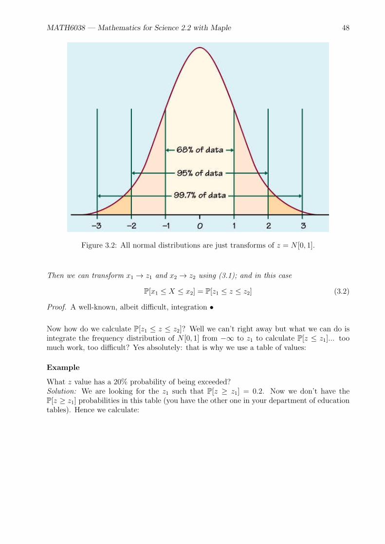
Figure 3.2: All normal distributions are just transforms of z = N [0, 1].
Then we can transform x1 → z1 and x2 → z2 using (3.1); and in this case
P[x1 ≤ X ≤ x2] = P[z1 ≤ z ≤ z2] (3.2)
Proof. A well-known, albeit difficult, integration •
Now how do we calculate P[z1 ≤ z ≤ z2]? Well we can’t right away but what we can do isintegrate the frequency distribution of N [0, 1] from −∞ to z1 to calculate P[z ≤ z1]... toomuch work, too difficult? Yes absolutely: that is why we use a table of values:
Example
What z value has a 20% probability of being exceeded?Solution: We are looking for the z1 such that P[z ≥ z1] = 0.2. Now we don’t have theP[z ≥ z1] probabilities in this table (you have the other one in your department of educationtables). Hence we calculate:

MATH6038 — Mathematics for Science 2.2 with Maple 49
Summer 2011 Question 3(d)
Samples of 10 A fuses have a mean fusing current of 9.9 A and a standard deviation of 1.2A. Assuming the fusing currents are normally distributed, determine the probability of a fuseblowing with a current between 8 A and 12 A.Solution:
Autumn 2011 Question 1(b)
Wires manufactured for use in a certain electronic device are specified to have resistancesbetween 0.16 Ω and 0.18 Ω. The actual measured resistances of the wires have a normal dis-tribution with a mean of 0.17 Ω and a standard deviation of 0.005 Ω. What is the probabilitythat a randomly selected wire will meet the specifications?Solution:
Autumn 2011 Question 2(b)
It is assumed that the weights of goods packed by a certain machine are normally distributedwith a mean weight of 8 kg and a standard deviation of 0.03 kg. Calculate the probabilitythat a package taken at random will weigh
1. less than 8.07 kg
2. greater than 8.08 kg
3. between 7.98 kg and 8.05 kg?
If 99.8% of readings are less than some critical weight, W , find the value of W .Solution:
3.9 Sampling
Consider the problem of finding the mean-average height, µ, of the population of Irish males.Plainly this is impossible. However we could approximate this population mean-average bytaking a random sample of say 1, 000 males from the population. Suppose we measure thesemales to have heights
h1, h2, . . . , h1,000.
We could then find the mean-average of the sample:
h =h1 + · · ·+ h1,000
h=
1
h
1,000∑i=1
hi,
Now we could take h as an estimate of µ; x ≈ µ. How accurate is this? Now consider all thepossible samples we could have taken from the population:So in this sense, the mean-average of the sample means is equal to the population mean. Wecan also show that the standard deviation of the sample means from the population meanis given by
√σ/
√1, 000, where σ is the standard deviation of the population.
This general process is called sampling and is used to make inferences of a whole populationjust by looking at a random sample of the data.
MATH6038 — Mathematics for Science 2.2 with Maple 50
3.9.1 The Central Limit Theorem
The Central Limit Theorem (CLT) is of crucial importance in sampling theory (as well asprobability theory in general). It essentially says that in many cases, a large collection of in-dependent identically distributed random variables has a normal distribution approximately.In particular this is true for the Binomial distribution:
limn→∞
B[n, p] → N [np,√
np(1− p)]. (3.3)
Example
A random variable has binonomial distribution with n = 200 and p = 0.2. Use the Normalapproximation X = B[200, 0.2] ≈ N [40,
√32] to estimate the probability P[30 < X < 45].
Solution: First we do a z-transforms of X = 30 and X = 45:
Hence we must calculate P[−1.77 < z < 0.88]:
As before, the best way to calculate this is to calculate
P[z ≤ 0.88]− 0.5 =
P[z ≤ 1.77]− 0.5 =
Much more importantly however is the role of CLT in Sampling Theory: it underpins thewhole justification.
Hence we can be reasonably confident of using sample summary statistics to estimate popu-lation summary statistics. Hence we can make informed and statistically significant decisions(recall the example in the motivation of how often to close down the production line).
MATH6038 — Mathematics for Science 2.2 with Maple 51
Example
The times taken to travel from your home to class on n = 7 different days are:
30, 33, 26, 23, 30, 35, 27 mins
If you are willing to take a 1% chance of being late for class, how long before the class shouldyou set out?Solution:
3.10 Quality Control Charts
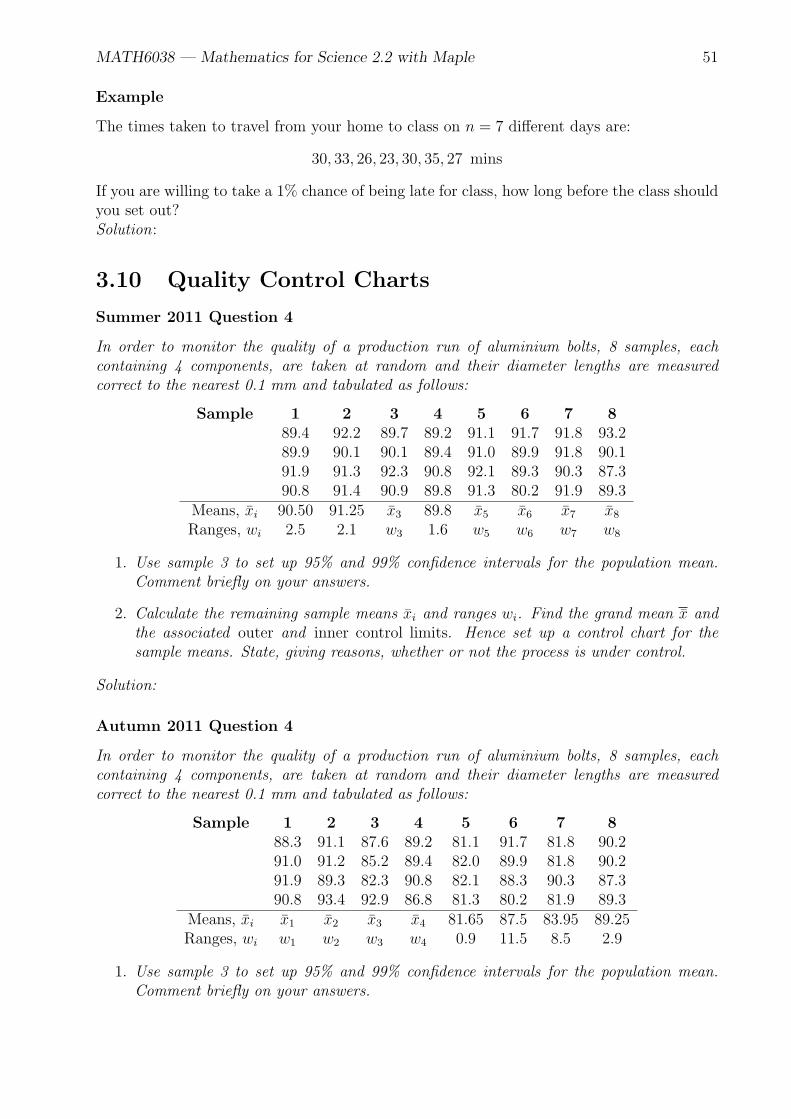
Summer 2011 Question 4
In order to monitor the quality of a production run of aluminium bolts, 8 samples, eachcontaining 4 components, are taken at random and their diameter lengths are measuredcorrect to the nearest 0.1 mm and tabulated as follows:
Sample 1 2 3 4 5 6 7 889.4 92.2 89.7 89.2 91.1 91.7 91.8 93.289.9 90.1 90.1 89.4 91.0 89.9 91.8 90.191.9 91.3 92.3 90.8 92.1 89.3 90.3 87.390.8 91.4 90.9 89.8 91.3 80.2 91.9 89.3
Means, xi 90.50 91.25 x3 89.8 x5 x6 x7 x8
Ranges, wi 2.5 2.1 w3 1.6 w5 w6 w7 w8
1. Use sample 3 to set up 95% and 99% confidence intervals for the population mean.Comment briefly on your answers.
2. Calculate the remaining sample means xi and ranges wi. Find the grand mean x andthe associated outer and inner control limits. Hence set up a control chart for thesample means. State, giving reasons, whether or not the process is under control.
Solution:
Autumn 2011 Question 4
In order to monitor the quality of a production run of aluminium bolts, 8 samples, eachcontaining 4 components, are taken at random and their diameter lengths are measuredcorrect to the nearest 0.1 mm and tabulated as follows:
Sample 1 2 3 4 5 6 7 888.3 91.1 87.6 89.2 81.1 91.7 81.8 90.291.0 91.2 85.2 89.4 82.0 89.9 81.8 90.291.9 89.3 82.3 90.8 82.1 88.3 90.3 87.390.8 93.4 92.9 86.8 81.3 80.2 81.9 89.3
Means, xi x1 x2 x3 x4 81.65 87.5 83.95 89.25Ranges, wi w1 w2 w3 w4 0.9 11.5 8.5 2.9
1. Use sample 3 to set up 95% and 99% confidence intervals for the population mean.Comment briefly on your answers.

MATH6038 — Mathematics for Science 2.2 with Maple 52
2. Calculate the remaining sample means xi and ranges wi. Find the grand mean x andthe associated outer and inner control limits. Hence set up a control chart for thesample means. State, giving reasons, whether or not the process is under control.
Solution:
3.11 Bayesian Statistics
Summer 2011 Question 1(e)(ii)
A technical supervisor picks a sample of 20 light bulbs at random from a shipment of lightbulbs known to contain 10% defective light bulbs. What is the probability that no more thantwo of the light bulbs are defective?
Remark
Solution:
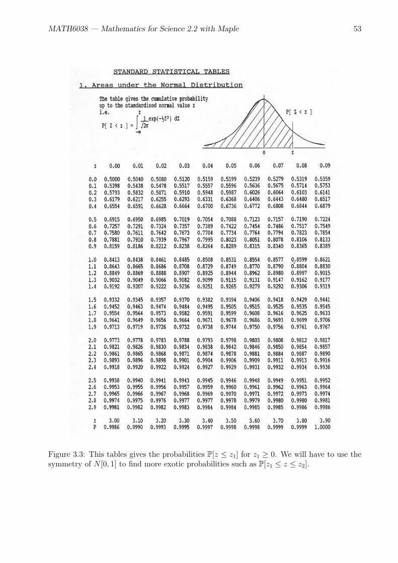
MATH6038 — Mathematics for Science 2.2 with Maple 53
Figure 3.3: This tables gives the probabilities P[z ≤ z1] for z1 ≥ 0. We will have to use thesymmetry of N [0, 1] to find more exotic probabilities such as P[z1 ≤ z ≤ z2].

MATH6038 — Mathematics for Science 2.2 with Maple 54
Figure 3.4: There are about 103733 possible samples of 1,000 males from the populationof about 2,000. If we look at the sample mean-average as a random variable, then themean-average of the sample mean-averages is equal to the population mean-average.