MATH1013 Calculus I

MATH1013 Calculus I

Revision1

Edmund Y. M. Chiang

Department of MathematicsHong Kong University of Science & Technology

November 27, 2014

1Based on Briggs, Cochran and Gillett: Calculus for Scientists and Engineers: Early Transcendentals, Pearson

2013

Functions Definition of functions Transformations Limits Derivatives Curve Sketching Fundamental Theorem of Calculus

Functions

Definition of functions

Transformations

Limits

Derivatives

Curve Sketching

Fundamental Theorem of Calculus


Definition of functions

• Definition A function is a rule f that assigns to each x in aset D a unique value denoted by f (x).

• Definitions The set D is called the domain of the function f ,and the set of values of f (x) assumes, as x varies over thedomain, is called the range of the function f (x).

•x 7−→ f (x), or y = f (x),

• One can think of this as a model of

one input → one output

• Important point: for each x in D, one can find (there exists)one value f (x) (or y) that corresponds to it.

• However, depending on the f under consideration, one couldhave two or more x that correspond to the same f (x).


Different types of functions

• y = f (x) = x + 1. For each x there corresponds to one andonly one y .

• y = x3. For each x there corresponds to one and only one y

• Where f (x1) = f (x2) implies x1 = x2, or equivalently x1 6= x2

implies f (x1) 6= f (x2), we say the function f is injective orone-one. So the above two examples are injective functions.

• (Eg revisited) f (x) = x2 − 2x is not injective, as two differentx can correspond to the same f (x1) = y = f (x2)

• (Non-function) y 2 = 1− x2. Since for each x input, therealways correspond to two outputs of f (x) = ±

√1− x2 within

the domain of f .


Composition

• Definition Given two functions f and g , their compositionf ◦ g is defined, by

(f ◦ g)(x) = f (u) = f (g(x))

for each x in the domain of f ◦ g . Let u = g(x) andy = f (u), then f ◦ g is understood as

y = (f ◦ g)(x) = f (g(x)) = f (u), u = g(x),

• as shown in

x 7−→ u = g(x) 7−→ y = f (u)

• with g takes the domain of g (range) into (part of) domain off , and f maps that into (part of) the range of f . The twotogether thus forms a new function f ◦ g .


Different classes of functions

• Polynomials, Rational fns.

• Exponential fns f (x) = 2x , f (x) = ex

• Logarithmic fns f (x) = ln x , f (x) = logx• trigonometric rations/fns sin x , cos x , tan x , etc

• Periodic properties

• Inverse trigonometric fns


Exponential functions of different bases

Figure: (Briggs, et al Figure 1.42)


Exponential functions



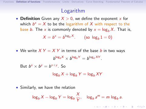
Logarithm• Definition Given any X > 0, we define the exponent x for

which bx = X to be the logarithm of X with respect to thebase b. The x is commonly denoted by x = logb X . That is,

X = bx = blogb X . (so logb 1 = 0)

• We write X Y = X Y in terms of the base b in two ways

blogbX × blogbY = blogb XY .

But bx × by = bx+y . So

logb X + logb Y = logb XY

• Similarly, we have the relation

logb X − logb Y = logbX

Y, logb am = m logb a.


Logarithm (change of bases)• How do these different logarithms for the same number X

relate to each other?• Suppose X is a given number, and

blogb X = X = c logc X

are the two different logarithms with respect to base b and crespectively.

• Taking logb on both sides yields

(logbX )(logb b︸︷︷︸=1

) = (logc X )(logb c)

That is, logb X/ logc X = logb c .• Similarly, Taking logc on both sides yields

(logbX )(logc b) = (logc X )(logc c︸︷︷︸=1

)

That is, logb X/ logc X = 1/ logc b.• So logb c = 1/ logc b.


Ratios as circular functions: 0 ≤ θ ≤ 2π• Due to the property of similar triangles, it is sufficient that we

consider unit circle in extending to 0 ≤ θ ≤ 2π with the ratiosaugmented with appropriate signs from the xy−coordinateaxes.

Figure: (Source: Bocher, page 38)


Ratios beyond 2π

• For sine and cosine functions, if θ is an angle beyond 2π, thenθ = φ+ k 2π for some 0 ≤ φ ≤ 2π. Thus one can write downtheir meanings from the definitions

sin(θ) = sin(φ+k 2π) = sinφ, cos(θ) = cos(φ+k 2π) = cosφ

where 0 ≤ φ ≤ 2π, and k is any integer.

• The case for tangent ratio is slightly different, with the firstextension to −π

2 ≤ θ ≤π2 , and then to arbitrary θ. Thus one

can write down

tan(θ) = tan(φ+ k π) = tanφ

where θ = φ+ kπ for some k and −π2 < φ < π

2 .


Periodic sine and cosine functions

Figure: (Source:Upper: sine, page 45; Lower: cosine, page 46)


Periodic tangent function

Figure: (Source: tangent, Bocher page 46)


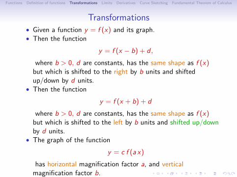
Transformations• Given a function y = f (x) and its graph.• Then the function

y = f (x − b) + d ,

where b > 0, d are constants, has the same shape as f (x)but which is shifted to the right by b units and shiftedup/down by d units.

• Then the function

y = f (x + b) + d

where b > 0, d are constants, has the same shape as f (x)but which is shifted to the left by b units and shifted up/downby d units.

• The graph of the function

y = c f (a x)

has horizontal magnification factor a, and verticalmagnification factor b.


Inverse functions

• Definition Let f be a function defined on its domain D. Thena function f −1 is called an inverse of f if

(f −1 ◦ f )(x) = x , for all x in D.

That is, x = f −1(y) whenever y = f (x).

• Remark 1 It follows that the domain of f −1 is on the rangeof f .

• Remark 2 There is no guarantee that every function has aninverse.

• Remark 3 If f has two inverse functions, then the two inversefunctions must be identically the same.


Inverse function figure



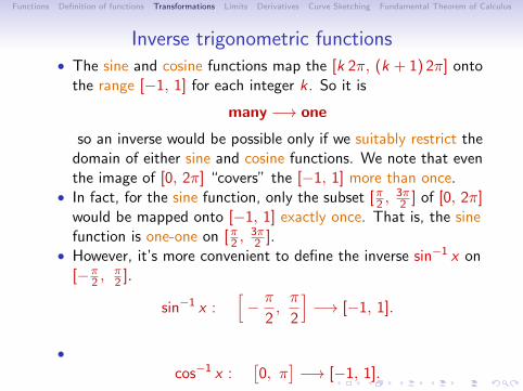
Inverse trigonometric functions• The sine and cosine functions map the [k 2π, (k + 1) 2π] onto

the range [−1, 1] for each integer k . So it is

many −→ one

so an inverse would be possible only if we suitably restrict thedomain of either sine and cosine functions. We note that eventhe image of [0, 2π] “covers” the [−1, 1] more than once.

• In fact, for the sine function, only the subset [π2 ,3π2 ] of [0, 2π]

would be mapped onto [−1, 1] exactly once. That is, the sinefunction is one-one on [π2 ,

3π2 ].

• However, it’s more convenient to define the inverse sin−1 x on[−π

2 ,π2 ].

sin−1 x :[− π

2,π

2

]−→ [−1, 1].

•cos−1 x :

[0, π

]−→ [−1, 1].


Logarithm as inverse function

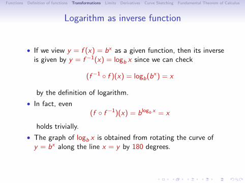
• If we view y = f (x) = bx as a given function, then its inverseis given by y = f −1(x) = logb x since we can check

(f −1 ◦ f )(x) = logb(bx) = x

by the definition of logarithm.

• In fact, even(f ◦ f −1)(x) = blogb x = x

holds trivially.

• The graph of logb x is obtained from rotating the curve ofy = bx along the line x = y by 180 degrees.


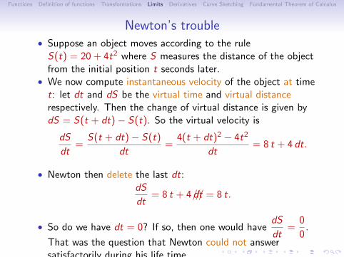
Newton’s trouble• Suppose an object moves according to the rule

S(t) = 20 + 4t2 where S measures the distance of the objectfrom the initial position t seconds later.

• We now compute instantaneous velocity of the object at timet: let dt and dS be the virtual time and virtual distancerespectively. Then the change of virtual distance is given bydS = S(t + dt)− S(t). So the virtual velocity is

dS

dt=

S(t + dt)− S(t)

dt=

4(t + dt)2 − 4t2

dt= 8 t + 4 dt.

• Newton then delete the last dt:dS

dt= 8 t + 4 dt/// = 8 t.

• So do we have dt = 0? If so, then one would havedS

dt=

0

0.

That was the question that Newton could not answersatisfactorily during his life time.


Newton’s thought

• So he simply considers that is a virtual distance dS traveledby the object in a virtual time dt. He considers both to beinfinitesimal small quantities.

• So do we have dt = 0? If so, then one would have dSdt = 0

0 .That was the question that Newton could not answersatisfactorily during his life time.

• To put the question differently, is an infinitesimal quantityequal to zero? If dt is infinitely small then it would have to beless than any positive quantity, and we conclude it must beequal to zero. For suppose dt 6= 0 then dt > 0. Hencedt = r > 0 is an actual positive quantity. But then we couldfind r/2 < dt, contradicting the fact that dt is smaller thenany positive quantity. Hence dt = 0.

• Newton was actually attacked by many people, and amongthem was the Bishop Berkeley. But the method of calculationof instantaneous velocity has been used by other since then.


Re-assessing the problem• Let us begin with the above example about the movement of

the object P. Since we are interested to know the magnitudeof the average velocity of P near 2, so let us rewrite theexpression in the following form:

g(x) =S(2 + x)− S(2)

x.

• This is a function g depends on the variable x , which can bemade as close to 16 as we wish by choosing t close to 2.

• That is, g(x) approaches the value 16 as x approaches 0. Onthe other hand, we cannot put x = 0 in the function g(x),since both the numerator S(2 + x)− S(x) and thedenominator x would be zero.

• We say that the function g has limit equal to 16 as xapproaches 0 abbreviated as

limx→0

g(x) = 16.


Limit definition

• Note that the above statement is merely an abbreviation forthe statement: The function g can get as close to 16 aspossible if we let x approach 0 as close as we wish.

• It is important to note that we are not allowed to put x = 0above

• Definition Let a and l be two real numbers. If the value ofthe function f (x) approaches l as close as we wish as xapproaches a, then we say the limit of f is equal to l as xtends to a. The statement is denoted by

limx→a

f (x) = l .

Alternatively, we may also write

f (x)→ l as x → a.


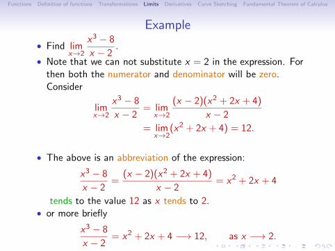
Example

• Find limx→2

x3 − 8

x − 2.

• Note that we can not substitute x = 2 in the expression. Forthen both the numerator and denominator will be zero.Consider

limx→2

x3 − 8

x − 2= lim

x→2

(x − 2)(x2 + 2x + 4)

x − 2

= limx→2

(x2 + 2x + 4) = 12.

• The above is an abbreviation of the expression:

x3 − 8

x − 2=

(x − 2)(x2 + 2x + 4)

x − 2= x2 + 2x + 4

tends to the value 12 as x tends to 2.• or more briefly

x3 − 8

x − 2= x2 + 2x + 4 −→ 12, as x −→ 2.


Illegal step

If

f (x) =x3 − 8

x − 2,

then it is absolutely forbidden to write

limx→2

f (x) =x3 − 8

x − 2= f (2)

since the function f is simply undefined at x = 2.


An example that has no limit

• Recall that the earlier example f (x) =

{2 if x 6= 1,

1 if x = 1.has no

limit at x = 1 which is a discontinuity of f . But we could stillcorrect f to be continuous at x = 1 again by re-definingf (1) = 2.

• Consider the example on page 64:

f (x) = cos1

x

on the interval (0, 1]. It is not defined at x = 0. We see thateven a small change in x near zero would result in a large

change of1

x.So there would be an unlimited number of

oscillations between the values {±1} throughout (0, a].Hence no correction of value of f (x) would make f (x)continuous at x = 0 again.


A function that has no limit at 0



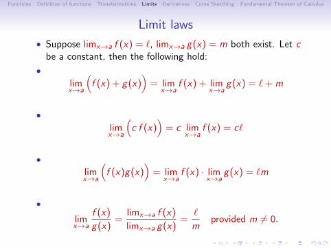
Limit laws

• Suppose limx→a f (x) = `, limx→a g(x) = m both exist. Let cbe a constant, then the following hold:

•limx→a

(f (x) + g(x)

)= lim

x→af (x) + lim

x→ag(x) = `+ m

•limx→a

(c f (x)

)= c lim

x→af (x) = c`

•limx→a

(f (x)g(x)

)= lim

x→af (x) · lim

x→ag(x) = `m

•

limx→a

f (x)

g(x)=

limx→a f (x)

limx→a g(x)=

`

mprovided m 6= 0.


The real difficulty

• We recall that in terms of ε− δ language limx→a f (x) = `really meansGiven an arbitrary ε > 0, one can find a δ > 0 such that

|f (x)− `| < ε, whenever 0 < |x − a| < δ.

• So for limx→a[f (x) + g(x)] = limx→a f (x) + limx→a g(x), oneneeds to show, assuming that limx→a g(x) = sGiven an arbitrary ε > 0, one can find a δ > 0 such that∣∣[f (x) + g(x)]− (`+ s)

∣∣ < ε, whenever 0 < |x − a| < δ.

with the given assumption.

• This is slightly not easy. Some other laws are more difficult toverify using this language. So this explains why one needs tostate these seemingly simple laws as separate entities.


Limits at infinity

• Definitions Let ` and a be real numbers. If f tends to ` as xbecomes arbitrary large and positive, we say f has the limit `at positive infinity, written as

limx→+∞

f (x) = ` (f → `, as x → +∞).

• Similarly, if f tends to ` as x becomes arbitrary large andnegative, we say f has the limit ` at negative infinity, writtenas

limx→−∞

f (x) = ` (f → `, as x → −∞).


Rate of change• We may consider rate of change of a given function f (x) not

necessarily refereed to time, distance and velocity.• Definition Let f (x) be a function of x , then f is differentiable

at x if the limit

lim∆x→0

∆f

∆x= lim

∆x→0

f (x + ∆x)− f (x)

∆x

exists.• The limit is called the derivative of f at x or the rate of

change of f with respect to x , and it is denoted by f ′(x).• Other notations are

df (x)

dxor

df

dx

∣∣∣∣x

ordf

dx

• If y = f (x), we also writedy

dx. We treat this notation as an

operator instead of quotient of infinitesimal quantities.• However, we shall see later that they are interchangeable.


Differentiation rules

• Theorem Let c be a constant and that a function f isdifferentiable at x . Then

d(c f )

dx= c

df

dxor (c f )′(x) = c f ′(x).

Proof Consider the following limit

lim∆x→0

cf (x + ∆x)− cf (x)

∆x= lim

∆x→0c( f (x + ∆x)− f (x)

∆x

)= c lim

∆x→0

f (x + ∆x)− f (x)

∆x.


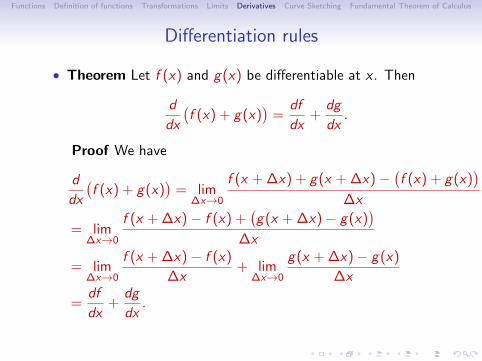
Differentiation rules

• Theorem Let f (x) and g(x) be differentiable at x . Then

d

dx

(f (x) + g(x)

)=

df

dx+

dg

dx.

Proof We have

d

dx

(f (x) + g(x)

)= lim

∆x→0

f (x + ∆x) + g(x + ∆x)−(f (x) + g(x)

)∆x

= lim∆x→0

f (x + ∆x)− f (x) +(g(x + ∆x)− g(x)

)∆x

= lim∆x→0

f (x + ∆x)− f (x)

∆x+ lim

∆x→0

g(x + ∆x)− g(x)

∆x

=df

dx+

dg

dx.


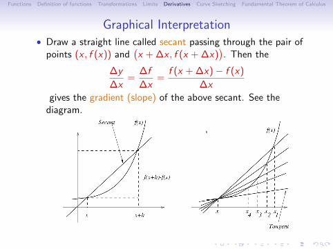
Graphical Interpretation• Draw a straight line called secant passing through the pair of

points (x , f (x)) and(x + ∆x , f (x + ∆x)

). Then the

∆y

∆x=

∆f

∆x=

f (x + ∆x)− f (x)

∆x

gives the gradient (slope) of the above secant. See thediagram.

Figure: (Secants and tangent)


Graphical Interpretation (cont.)• We choose ∆x1, ∆x2, ∆x3, . . . with magnitudes decreasing to

zero. Then we have a sequence of secants passing through thepoints

((x , f (x)

),(f (x + ∆xi )

).

• The corresponding gradients of the secants are given by

mi =f (x + ∆xi )− f (x)

∆xi.

• Suppose we already know that f has a derivative at x , weconclude that the sequence of gradients {mi} must tend tof ′(x) as ∆xi tends to zero.

• The point(x + ∆x , f (x + ∆x)

)is getting closer and closer to(

x , f (x)), as ∆x → 0, they eventually coincide to become a

single point.• It follows that the corresponding secants are tending to a

straight line with only one point of contact with f at x . Seethe diagram from last slide. This line is called the tangent tof at x .


An example has no tangent

• Example The |x | is not differentiable at 0.

• Consider

lim∆x→0+

|0 + ∆x | − |0|∆x

= lim∆x→0+

|∆x |∆x

= lim∆x→0+

∆x

∆x= 1.

• On the other hand, we have, according to the definition of |x |that

lim∆x→0−

|0 + ∆x | − |0|∆x

= lim∆x→0−

|∆x |∆x

= lim∆x→0−

−∆x

∆x= −1.

• So the left and right limits are not the same, and we concludethat |x | does not have a derivative at 0 (however, it hasderivatives at all other points). It is important to understandthe corresponding situation on its graph drawn on last slide(right figure).


Last example’s sketch

It is instructive to plot the curve of P and P ′ on the samecoordinate axis. See the diagram on the left below.

Figure: (Left: Profit function; Right: |x | has no tangent at 0)


How does composition change?

• Suppose that y = g(u) and u = f (x). i.e., is y is a functionof u and u is a function of x .

• When we compose to get y = g(f (x)), which is now afunction of x , written as y = h(x).

• If x is changed to x + ∆x , there’s a corresponding change inu,

u + ∆u = f (x + ∆x).

• As a result, it will induce a further change in y . Hence

y + ∆y = g(u + ∆u).


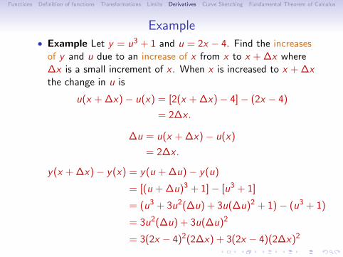
Example• Example Let y = u3 + 1 and u = 2x − 4. Find the increases

of y and u due to an increase of x from x to x + ∆x where∆x is a small increment of x . When x is increased to x + ∆xthe change in u is

u(x + ∆x)− u(x) = [2(x + ∆x)− 4]− (2x − 4)

= 2∆x .

∆u = u(x + ∆x)− u(x)

= 2∆x .

y(x + ∆x)− y(x) = y(u + ∆u)− y(u)

= [(u + ∆u)3 + 1]− [u3 + 1]

= (u3 + 3u2(∆u) + 3u(∆u)2 + 1)− (u3 + 1)

= 3u2(∆u) + 3u(∆u)2

= 3(2x − 4)2(2∆x) + 3(2x − 4)(2∆x)2


Chain Rule

• Theorem Let y = g(u), u = f (x) and b = f (a), c = g(b).Suppose that g is differentiable at u = b, and that f isdifferentiable at x = a. Then the function y = h(x) = g(f (x))is also differentiable at x = a, and the relationship is given by

dh

dx

∣∣∣∣x=a

=dg

du

∣∣∣∣u=b

× df

dx

∣∣∣∣x=a

,

ordy

dx

∣∣∣∣x=a

=dy

du

∣∣∣∣u=b

× du

dx

∣∣∣∣x=a

,

or simplydy

dx=

dy

du× du

dx.


First Order Approximation

• When f is differentiable at x , the quotient

∆f

∆x=

f (x + ∆x)− f (x)

∆x

is very close to f ′(x), provided that ∆x is taken to be small.See the diagram. Hence we have

∆f

∆x≈ dy

dx= f ′(x).

In other words, we have

∆f = f (x + ∆x)− f (x) ≈ dy

dx∆x = f ′(x)∆x ,

i.e., the change in f due to a small change ∆x at x can beapproximated by f ′(x)∆x .


∆f ≈ f ′(x)∆x ,

•• In particular, when ∆x = 1, we have

∆f ≈ f ′(x),

• That is, the f ′(x) approximates the change of f (x) when x isincreased by one unit.


First Order Approximation

• Example Suppose y = f (x) = x2. Find an approximatechange of f (x) when x is increased from 2 to 2.5.

• We have f ′(x) = 2x . And f ′(2) = 2(2) = 4. Hence

∆y = y(2 + 0.5)− y(2) ≈ y ′(2) (0.5) = 4 (0.5) = 2.

Note that the real change of y can be computed directly byy(2.5)− y(2) = 2.25. The approximation will become moreaccurate if we involve changes much smaller than 0.5.

• Exercise Repeat the above example when x is increasedfrom 2 to 2.005. How accurate is it?

• Exercise Without using the calculus find an approximatevalue of 3.981/2.


Application: Marginal Analysis

• Economists are interested in the change f (x + 1)− f (x).Suppose that f is differentiable at x , then the first orderapproximation gives

∆f = f (x + 1)− f (x) ≈ f ′(x) ∆x = f ′(x),

i.e., the f ′(x) approximates the change in f , when x isincreased by 1 (assuming f is well-behaved). The above iscalled marginal analysis by economists.

• Let c(q) and r(q) = qp(q) to denote total cost function andtotal revenue function respectively (the p(q) is the pricefunction). Then

c ′(q) =dc

dq, and r ′(q) =

dr

dq

are called the marginal cost and marginal revenuerespectively.


More Rules for Differentiation

• Theorem Suppose f is differentiable at a then f must also becontinuous at a.

• Theorem Let f (x) and g(x) both be differentiable at x .Then

d(fg)

dx= g(x)

df (x)

dx+ f (x)

dg(x)

dx.

• Theorem Let f (x) and g(x) both be differentiable at x andthat g ′(x) 6= 0. Then

d

dx

(f

g(x)

)=

g(x)f ′(x)− f (x)g ′(x)

g(x)2.


Logarithmic functions• Recall that the natural logarithmic function log x is defined to

be the inverse function of the exponential function y = ex .That is x = ln(ex) and x = e ln x .

• Theorem. We have, for any x > 0,

d

dxln x =

1

x.

ln(x + h)− ln x

h=

1

hln(1 +

h

x

)= ln

(1 +

h

x

)1/h

= ln(1 +

1/x

k

)k→ ln(e1/x)

=1

xas k → +∞ (equivalent to h→ 0).

• Theorem Let u be a function of x . Thend

dxln u =

1

u

du

dx.


Different bases

• Theorem Let a be any positive real number. Then

d

dxloga x =

1

ln a

1

x.

Similarly, if u is a function of x , then

d

dxloga u =

1

u ln a

du

dx.

• Example Find the derivative of y = log3(x2 + 1)

dy

dx=

2x

(x2 + 1) ln 3


Differentiation of trigonometric functions

• We omit the proof of cos′ x = − sin x .

• When sin x reaches its maxima/minima, 0 = sin′ x = cos x .That is, when

x =(2n + 1)π

2, n = 0, ±1,±2, ±3, · · ·

• Exercises Where are the maxima/minima of cos x?(p. 164)(1 + sin x

1− sin x

)′, tan′ x = sec2 x , cot′ x = − csc2 x

sec′ x = sec x tan x , csc′ x = − csc x cot x , (ex sin x)′.


Derivative of inverseTheorem (p. 215) Let f be differentiable and have an inverse onan interval I . If x0 is in I such that f ′(x0) 6= 0, then f −1 isdifferentiable at y0 = f (x0) and

(f −1)′(y0) =1

f ′(x0).

Proof Since x0 = f −1(y0) and x = f −1(y) so

(f −1)′(y0) = limy→y0

f −1(y)− f −1(y0)

y − y0

= limy→y0

x − x0

f (x)− f (x0)

= limx→x0

1f (x)−f (x0)

x−x0

=1

f ′(x0)

since (f −1) is continuous. In particular, we note thatf ′(x0)(f −1)′(y0) = 1.


Figure 3.65 (Briggs, et al)


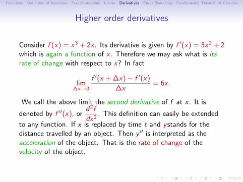
Higher order derivatives

Consider f (x) = x3 + 2x . Its derivative is given by f ′(x) = 3x2 + 2which is again a function of x . Therefore we may ask what is itsrate of change with respect to x? In fact

lim∆x→0

f ′(x + ∆x)− f ′(x)

∆x= 6x .

We call the above limit the second derivative of f at x . It is

denoted by f ′′(x), ord2f

dx2. This definition can easily be extended

to any function. If x is replaced by time t and ystands for thedistance travelled by an object. Then y ′′ is interpreted as theacceleration of the object. That is the rate of change of thevelocity of the object.


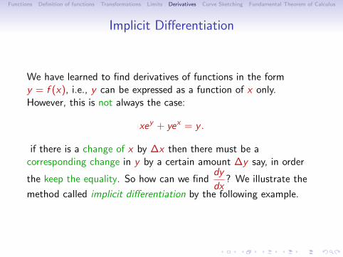
Implicit Differentiation

We have learned to find derivatives of functions in the formy = f (x), i.e., y can be expressed as a function of x only.However, this is not always the case:

xey + yex = y .

if there is a change of x by ∆x then there must be acorresponding change in y by a certain amount ∆y say, in order

the keep the equality. So how can we finddy

dx? We illustrate the

method called implicit differentiation by the following example.


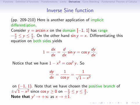
Inverse Sine function

(pp. 209-210) Here is another application of implicitdifferentiation.Consider y = arcsin x on the domain [−1, 1] has range−π

2 ≤ y ≤ π2 . On the other hand sin y = x . Differentiating this

equation on both sides yields

1 =dx

dx=

d

dxsin y = cos y

dy

dx.

Notice that we have 1− x2 = cos2 y . So

dy

dx=

1

cos y=

1√1− x2

on (−1, 1). Note that we have chosen the positive branch of±√

1− x2 since cos y ≥ 0 on −π2 ≤ y ≤ π

2 .Note that y ′ → +∞ as x → ±1.


Maximum/Minimum

We see the drawing (Briggs, et al, p. 259) below that

• At some local maximum/minimum, f ′(x) = 0.

• f (x) may fail to have derivative at certain localmaximum/minimum, such as the point c where f ′(c) fails toexist.

• In a finite interval [a, b], f may have globalmaximum/minimum.


At extrema

• Definition We call x = a a critical point of f if f ′(a) = 0.

• If f has a maximum or a minimum at a, then f ′(a) = 0 is acritical point.

• The converse is not necessarily true.• That is, at a critical point a (f ′(a) = 0) may not represent

f (a) has either a maximum or minimum there.• Example f (x) = x3 + 2 has f ′(0) = 0 but f (0) is neither a

maximum nor a minimum.• Example f (x) = x4 has f ′(0) = 0 and f (0) is a maximum

• That is, knowing f ′(a) = 0 is insufficient to decide if f (a) isan extrema.


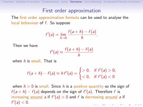
First order approximationThe first order approximation formula can be used to analyse thelocal behaviour of f . So suppose

f ′(a) = limh→0

f (a + h)− f (a)

h.

Then we have

f ′(a) ≈ f (a + h)− f (a)

h

when h is small. That is

f (a + h)− f (a) ≈ h f ′(a) =

{> 0, if f ′(a) > 0;

< 0, if f ′(a) < 0

when h > 0 is small. Since h is a positive quantity so the sign off (a + h)− f (a) depends on the sign of f ′(a). Therefore f isincreasing around a if f ′(a) > 0 and f is decreasing around a iff ′(a) < 0.


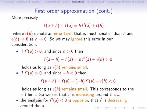
First order approximation (cont.)More precisely,

f (a + h)− f (a) = h f ′(a) + ε(h)

where ε(h) denote an error term that is much smaller than h andε(h)→ 0 as h→ 0. So we may ignore this error in ourconsideration.

• If f ′(a) > 0, and since h > 0 then

f (a + h)− f (a) = h f ′(a) + ε(h) > 0

holds as long as ε(h) remains small.• If f ′(a) > 0, and since −h < 0 then

f (a− h)− f (a) = (−h) f ′(a) + ε(h) < 0

holds as long as ε(h) remains small. This corresponds to theleft limit. So we see that f is increasing around the a.

• the analysis for f ′(a) < 0 is opposite, that f is decreasingaround the a.


First order derivative test

We have seen that around a critical point a being amaximum/minimum, the derivative f ′(x) changes signs. That is,

• when f (a) is a local maximum,

f ′(x)

> 0, if x < a;

= 0, if x = a;

< 0, if x > a.

f ′ ↓ that is ↗−→↘• when f (a) is a local minimum,

f ′(x)

< 0, if x < a;

= 0, if x = a;

> 0, if x > a.

f ′ ↑ that is ↘−→↗


First order derivative test: Converse statementsIt is not difficult to see that the converses also hold if x = a is acritical point: f ′(a) = 0. That is,• if f ′(x) decreases from being positive to being negative, then

f (a) is a local maximum;• if f ′(x) increases from being negative to being positive, then

f (a) is a local minimum


Example (p. 270 Briggs, et al)Let f (x) = 3x4 − 4x3 − 6x2 + 12x + 1. Find the intervals ofincrease/decrease and any local extrema of f .

f ′(x) = 12(x + 1)(x − 1)2 =

< 0, if x < −1;

> 0, if − 1 < x < 1;

> 0, if x > 1.


Concavity I (Briggs, et al)• Definition A differentiable function f is concave up over an

interval I if f ′ is increasing over I .• Definition A differentiable function f is concave down over

an interval I if f ′ is decreasing over I .


Concavity II

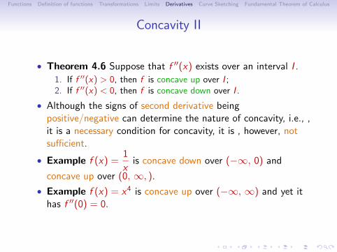
• Theorem 4.6 Suppose that f ′′(x) exists over an interval I .

1. If f ′′(x) > 0, then f is concave up over I ;2. If f ′′(x) < 0, then f is concave down over I .

• Although the signs of second derivative beingpositive/negative can determine the nature of concavity, i.e., ,it is a necessary condition for concavity, it is , however, notsufficient.

• Example f (x) =1

xis concave down over (−∞, 0) and

concave up over (0, ∞, ).

• Example f (x) = x4 is concave up over (−∞, ∞) and yet ithas f ′′(0) = 0.


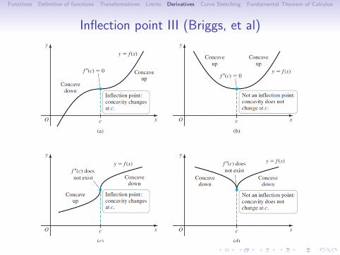
Inflection point I

• Definition A point c is called a point of inflection for afunction f (x) if f (x) is continuous at a and if there is achange of concavity:

• That is, if

f ′′(x) > 0, x < c ;

f ′′(x) < 0, x > c ,

• or

f ′′(x) < 0, x < c ;

f ′′(x) > 0, x > c .

• Depending on the behaviour of f (x) at the inflection point, itssecond derivative could be zero there, i.e., f ′′(c) = 0 or f ′′(c)simply undefined.


Inflection point II

• If f (x) has an inflection point at x = c and that f ′′(x) iscontinuous over an interval containing x = c , then f ′′(c) = 0.

• Example f (x) = x3 has an inflection point at x = 0 sincethere is a change of concavity and f ′′(0) = 0.

• Example f (x) = −x3 has an inflection point at x = 0 sincethere is a change of concavity and f ′′(0) = 0.

• Remark Even if f ′′(x) is continuous around x = c , andf ′′(0) = 0, it does not imply necessarily that f (x) has aninflection point at x = c .

• Example f (x) = x4 is concave up over (−∞, ∞) andalthough f ′′(x) > 0 whenever x 6= 0, yet it has f ′′(0) = 0.

• f ′′(0) = 0 it is a necessary condition for concavity, it is ,however, not sufficient.

• The next slide shows that f ′′ is undefined at a point ofinflection.


Inflection point III (Briggs, et al)


Example (Briggs, et al, p. 274) I

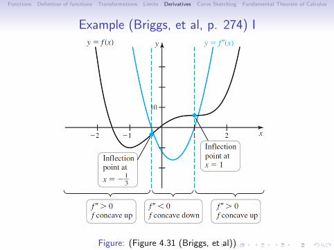
Identify the intervals of concave up/down off (x) = 3x4 − 4x3 − 6x2 + 12x + 1.We have already computed

f ′(x) = 12(x + 1)(x − 1)2 =

< 0, if x < −1;

> 0, if − 1 < x < 1;

> 0, if x > 1.

f ′′(x) = 12(x − 1)(3x + 1)

> 0, if x < −1/3 or x > 1;

= 0, if x = −1/3 or x = 1;

< 0, if − 1/3 < x < 1;

We deduce that the critical points are {−1, 1} and the inflectionpoints are {−1/3, 1}.


Example (Briggs, et al, p. 274) I

Figure: (Figure 4.31 (Briggs, et al))


Example IISketch the graph of y = f (x) = x +

4

x + 1.

• The easiest is to find the where f intersects with with theaxes. Suppose f (x) = 0, i.e., 0 = x + 4

x+1 or x2 + x + 4 = 0

x =−1±

√14 − 4· 1· 42

,

which has no solution since 12 − 16 < 0. So f will never bezero, and so f will never intersect the x−axis. Besides,f (0) = 4.

• The next step is to consider x → +∞ and x → −∞.When x is large and positive f (x)− x is approaching zero.i.e.,

limx→+∞

(f (x)− x

)= lim

x→+∞

( 4

x + 1

)= 0.

Similarly,

limx→−∞

(f (x)− x

)= lim

x→−∞

( 4

x + 1

)= 0.


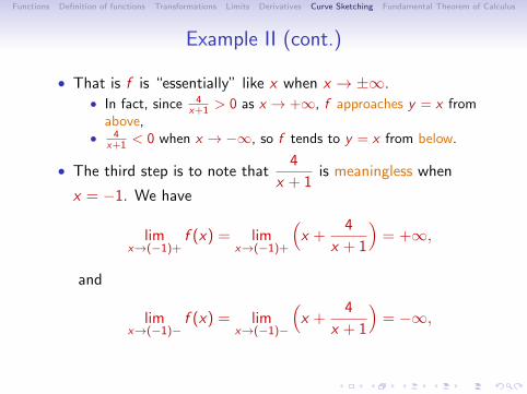
Example II (cont.)

• That is f is “essentially” like x when x → ±∞.• In fact, since 4

x+1 > 0 as x → +∞, f approaches y = x fromabove,

• 4x+1 < 0 when x → −∞, so f tends to y = x from below.

• The third step is to note that4

x + 1is meaningless when

x = −1. We have

limx→(−1)+

f (x) = limx→(−1)+

(x +

4

x + 1

)= +∞,

and

limx→(−1)−

f (x) = limx→(−1)−

(x +

4

x + 1

)= −∞,


Example II (cont.)

• The fourth step is to identify the critical points.

f ′(x) = 1− 4

(x + 1)2=

(x − 1)(x + 3)

(x + 1)2

=

> 0, if x < −3;

< 0, if − 3 < x < −1;

< 0, if − 1 < x < 1

> 0, if x > 1.

We deduce f has a maximum at x = −3 and a minimum atx = 1. In fact, f is increasing on the intervals x < −3 andx > 1, and decreasing on the intervals −3 < x < −1 and−1 < x < 1.


Example II (cont.)

• Now the concavity f ′′(x) =8

(x + 1)3=

{> 0, if x > −1;

< 0 if x < −1.


Extreme Value theorem

• Theorem A function f (x) continuous on a closed interval[a, b] attains its absolute maximum/minimum on [a, b]. Thatis, there exist c , d in [a, b] such that

f (x) ≥ f (c), f (x) ≤ f (d) for all x in [a, b].

• This result looks very trivial is in fact a deep result inelementary mathematical analysis. It is proved vigorously inchapter 5 (Theorem 5.3) of my supplementary notes onMathematical Analysis course found in my web site of thiscourse.

• What we will do in the following sides is to show the ExtremeValue theorem does not hold when any one of the hypothesesfails to hold.


Mean Value theoremTheorem If f is continuous on the closed interval [a, b] anddifferentiable on (a, b), then there is a c in [a, b] such that

f ′(c) =f (b)− f (a)

b − a.



Consequences of Mean Value theorem

• Theorem If f ′(x) = 0 at all points of an interval I , then f isa constant on I .

• Theorem If two functions have the property thatf ′(x) = g ′(x) on I , then f (x) = g(x) + k holds for all x in Ifor some constant k .

• Theorem Suppose f (x) is continuous on an interval I anddifferentiable at all interior points of I , then

• if f ′(x) > 0 at all interior points of I , then f is increasing on I ;• if f ′(x) < 0 at all interior points of I , then f is decreasing on I .


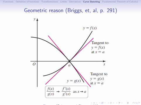
L’Hoptial’s rule 0/0 form

• Theorem (Briggs, et, al, ) Suppose f and g aredifferentiable on (a, b) and c lies in (a, b) such thatlimx→c f (x) = 0 = limx→c g(x) and g ′(x) 6= 0 (x 6= c) . Then

limx→c

f (x)

g(x)= lim

x→c

f ′(x)

g ′(x)

provided that the last limit exists.

• Remarks The above also holds for x → ±∞ or x → c±.

• Example

limx→0

sin x

x= lim

x→0

cos x

1=

limx→0 sin x

limx→0 1= 1.


Geometric reason (Briggs, et, al, p. 291)



“∞/∞” formTheorem (Briggs, et, al, p.319) Suppose f and g aredifferentiable on (a, b) and c lies in (a, b) such thatlimx→c f (x) = ±∞ = limx→c g(x) and g ′(x) 6= 0 (x 6= c) . Then

limx→c

f (x)

g(x)= lim

x→c

f ′(x)

g ′(x)

provided that the last limit exists.

Remark The above also holds for x → ±∞ or x → c±.

• Example limx→∞

4x3 − 6x2 + 1

2x3 − 10x + 3

• Example limx→π/2−

1 + tan x

sec x


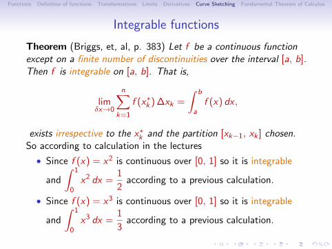
Integrable functions

Theorem (Briggs, et, al, p. 383) Let f be a continuous functionexcept on a finite number of discontinuities over the interval [a, b].Then f is integrable on [a, b]. That is,

limδx→0

n∑k=1

f (x∗k ) ∆xk =

∫ b

af (x) dx ,

exists irrespective to the x∗k and the partition [xk−1, xk ] chosen.So according to calculation in the lectures

• Since f (x) = x2 is continuous over [0, 1] so it is integrable

and

∫ 1

0x2 dx =

1

2according to a previous calculation.

• Since f (x) = x3 is continuous over [0, 1] so it is integrable

and

∫ 1

0x3 dx =

1

3according to a previous calculation.


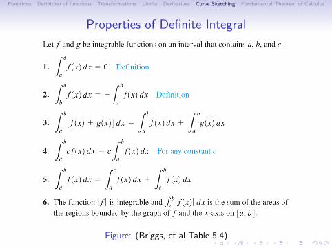
Properties of Definite Integral

Figure: (Briggs, et al Table 5.4)


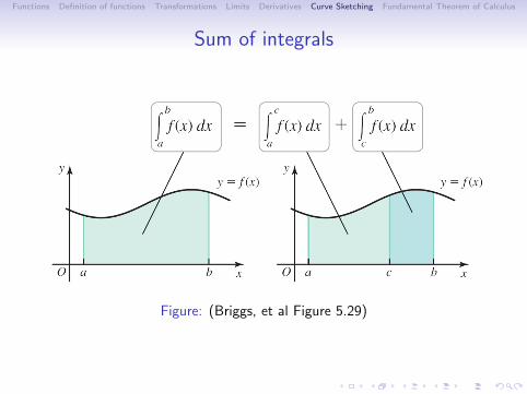
Sum of integrals



Fundamental theorem of calculus (Issac Newton)

Theorem 5.3 Suppose that f is continuous over [a, b] and that fhas a primitive (antiderivative) F (x) over [a, b], that is,F ′(x) = f (x) on [a, b]. Then∫ b

af (x) dx = F (x)

∣∣∣∣ba

= F (b)− F (a).

Example Find∫ 3

2 x2 dx by Newton’s Fundamental theorem ofcalculus.Since F (x) = 1

3 x3 is a primitive of f (x) = x2, so∫ 3

2x2 dx = F (3)− F (2) =

1

333 − 1

323 =

19

3.


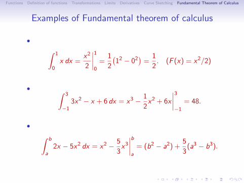
Examples of Fundamental theorem of calculus

• ∫ 1

0x dx =

x2

2

∣∣∣∣10

=1

2

(12 − 02

)=

1

2. (F (x) = x2/2)

• ∫ 3

−13x2 − x + 6 dx = x3 − 1

2x2 + 6x

∣∣∣∣3−1

= 48.

• ∫ b

a2x − 5x2 dx = x2 − 5

3x3

∣∣∣∣ba

= (b2 − a2) +5

3(a3 − b3).


Example on Derivatives of integral (Briggs, et, al, p. 400)

Given f (x) on [a, b], we recall from the proof of the Fundamentaltheorem of calculus that the area function defined by

F (x) =

∫ x

af (t) dt

serves as a primitive of f . That is, F ′(x) = f (x).So we have

(1)d

dx

(∫ x

1sin2 t dt

)= sin2 x .


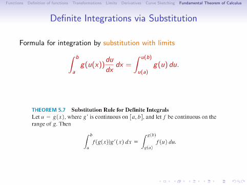
Definite Integrations via Substitution

Formula for integration by substitution with limits∫ b

ag(u(x))

du

dxdx =

∫ u(b)

u(a)g(u) du.


Definite Integrations via Substitution examples (Briggs, et,al, p. 419)

1. ∫ π/2

0sin4 x cos x dx =

∫ 1

0u4 du =

u5

5

∣∣∣10

=1

5.

2. ∫ 4

0

x

x2 + 1dx =

1

2

∫ 17

1

1

udu

=1

2ln |u|

∣∣∣117

=1

2(ln 17− ln 1).


Definite Integrations via Substitution examples (Briggs, et,al, p. 420)

1. ∫ 2

02(2x + 1) dx =

∫ 5

1u du =

u2

2

∣∣∣51.

MATH1013 Calculus I

Documents

Transcript of MATH1013 Calculus I