Math Review Session - cs5785-2019.github.io
40
Math Review Session CS5785, 2019 Fall Yichun Hu, Xiaojie Mao Cornell Tech, Cornell Unviersity
Transcript of Math Review Session - cs5785-2019.github.io

Math Review Session
CS5785, 2019 Fall
Yichun Hu, Xiaojie Mao
Cornell Tech, Cornell Unviersity

Table of contents
1. Linear Algebra
2. Calculus
3. Probability
4. Resources
1
Linear Algebra

Matrix and Vector
• Vector:
a =
1
2
3
, b =[1 2 3
]• Matrix:
A =
1 4 7
2 5 8
3 6 9
.• Vectorize a matrix:
vec(A) =
1
2
3
4...
9
.
2

Vector Operation
For two column vectors v , u ∈ Rn,
• Inner product: u · v = u>v =∑n
i=1 uivi .
• Orthogonal vectors: u · v = 0.
• Norm: ‖u‖ =√u>u =
√∑ni=1 u
2i .
• Euclidean distance: d(u, v) = ‖u − v‖ =√∑n
i=1(ui − vi )2.
3

Matrix Operation
• Transpose. For A ∈ Rm×n, A> is a n ×m matrix:
(A>)ij = Aji .
• Matrix addition. For A ∈ Rm×n, B ∈ Rm×n, C = A + B is a m × n
matrix: for 1 ≤ i ≤ m and 1 ≤ j ≤ n,
Cij = Aij + Bij .
• Matrix Multiplication. For A ∈ Rm×n, B ∈ Rn×p, C = AB is a
m × p matrix: for 1 ≤ i ≤ m and 1 ≤ j ≤ n,
Cij =n∑
k=1
AikBkj = Ai,: · B:,j
4

Matrix Operation
• Matrix inverse. If A is square (n × n), and invertible, then A−1 is
the unique n × n matrix such that
AA−1 = A−1A = I .
• Matrix trace. If A is square (n × n), then its trace is
tr(A) =n∑
i=1
Aii .
• Frobenius norm: for a matrix A ∈ Rm×n,
‖A‖F =
√√√√ m∑i=1
n∑j=1
A2ij =
√tr(A>A) = ‖ vec (A)‖.
5

Properties of Matrix Operation
• Transpose:
• (AB)> = B>A>.
• (ABC)> = C>B>A>.
• (A+ B)> = A> + B>.
• Multiplication:
• Associative: (AB)C = A(BC).
• Distributive: (A+ B)C = AC + BC .
• Non-commutative: AB 6= BA in general.
6

Properties of Matrix Operation
• Inverse:
• (AB)−1 = B−1A−1.
• (ABC)−1 = C−1B−1A−1.
• (A−1)−1 = A.
• (A−1)> = (A>)−1.
• Trace:
• tr(AB) = tr(BA).
• tr(ABC) = tr(CAB) = tr(BCA).
7

Special matrices
For A ∈ Rn×n,
• Diagonal matrix: Aij = 0 for any i 6= j .
• Symmetric (Hermitian) matrix: A = A> or Aij = Aji .
• Orthogonal matrix: A> = A−1.
• AA> = A>A = I .
• Rows and Columns are orthogonal unit vectors, namely, for i 6= j ,
Ai,: · Aj,: = 0, A:,i · A:,j = 0,
and for any i ,
Ai,: · Ai,: = 1, A:,i · A:,i = 1.
• Positive semidefinite matrix: for any x ∈ Rn with x 6= 0,
x>Ax =n∑
i=1
n∑j=1
Aijxixj ≥ 0.
8

Eigenvalues and Eigenvectors
For matrix A ∈ Rn×n, and nonzero vector u ∈ Rn (u 6= 0) such that
Au = λu,
u is an eigenvector of A, and λ is the corresponding eigenvalue.
9

Spectral decomposition theorem
If A ∈ Rn×n is a real symmetric matrix, then
A = UΛU> ⇔ A =n∑
i=1
λiuiu>i ⇔ U>AU = Λ
where
• U ∈ Rn×n is an orthogonal matrix whose columns are eigenvectors
of A, i.e., U:,i and U:,j are orthogonal unit eigenvectors for i 6= j .
• Λ is a diagonal matrix whose entries are the corresponding
eigenvalues.
Remark:
• tr(A) =∑n
i=1 λi .
• Real symmetric A is positive semidefinite ⇔ λi ≥ 0 for any
i = 1, . . . , n.
10

Singular Value Decomposition (SVD)
For A ∈ Rm×n, its singular value decomposition is
A = UΣV> ⇔ A =r∑
i=1
σiuiv>i ⇔ U>AV = Σ
where
• U ∈ Rm×r is an orthogonal matrix whose columns uiri=1 are the
left singular vectors;
• V ∈ Rr×n is an orthogonal matrix whose columns viri=1 are the
right singular vectors;
• Σ ∈ Rr×r is a diagonal matrix whose diagonal elements σiri=1 are
singular values.
11

Singular Value Decomposition
Remark:
• r is the rank of matrix A;
• The maximum singular value σmax(A) is called the spectral norm of
A, which we denote as ‖A‖2.
• Connection between SVD and eigen-decomposion.
A = UΣV> ⇒ AA> = UΣ2U>,
A = UΣV> ⇒ A>A = VΣ2V>.
Thus
• The columns of U are eigenvectors of AA>, and the columns of V
are eigenvectors of A>A;
• σ2i (A) = λi (AA
>) = λi (A>A).
12

Calculus
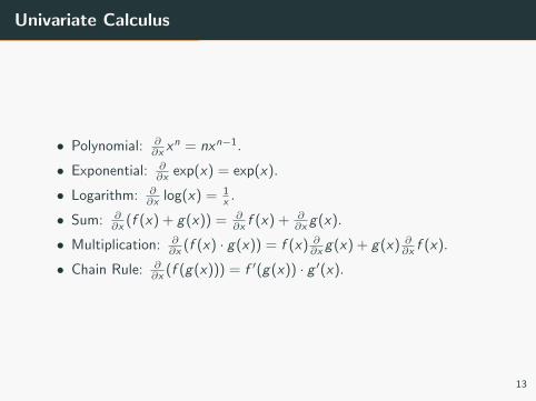
Univariate Calculus
• Polynomial: ∂∂x x
n = nxn−1.
• Exponential: ∂∂x exp(x) = exp(x).
• Logarithm: ∂∂x log(x) = 1
x .
• Sum: ∂∂x (f (x) + g(x)) = ∂
∂x f (x) + ∂∂x g(x).
• Multiplication: ∂∂x (f (x) · g(x)) = f (x) ∂
∂x g(x) + g(x) ∂∂x f (x).
• Chain Rule: ∂∂x (f (g(x))) = f ′(g(x)) · g ′(x).
13

Multivariate Calculus
Let f be a function of x1, x2, . . . , xn.
• Partial derivative ∂∂xi
f (x1, . . . , xn): treat other variables as
constants and take derivative w.r.t. xi .
∂
∂xf :=
∂f∂x1
. . .∂f∂xn
,∂
∂x>f :=
(∂f∂x1
. . . ∂f∂xn
)• Gradient of f with respect to x : ∇x f := ∂
∂x f .
• Hessian matrix of f : H is a n × n matrix with Hij = ∂2
∂xi∂xjf , or
H =∂2
∂x∂x>f .
Let f = (f1, . . . , fm) be a multivariate vector function of x1, . . . , xn.
• Jacobian matrix of f : J is a m × n matrix with Jij = ∂fi∂xj
. The
i-th row of J is ∂∂x> fi .
14

Multivariate Calculus Rules
Here a and A are vector/matrix that do not depend on x = (x1, . . . , xn)ᵀ.
• ∂∂x a = 0;
• ∂∂x a
ᵀx = ∂∂x x
ᵀa = a;
• ∂∂x (xᵀa)2 = 2aaᵀx;
• ∂∂xAx = A>;
• ∂∂x x
ᵀA = A;
• ∂∂x x>Ax = (Aᵀ + A)x.
For a detailed multivariate derivatives list, see
https://www.math.uwaterloo.ca/~hwolkowi/matrixcookbook.pdf.
15

Example: Least Squares
Lets apply the equations to derive the least squares equations. Suppose
we are given matrices A ∈ Rm×n (for simplicity we assume A is full rank
so that (A>A)−1 exists) and a vector b ∈ Rm such that b 6∈ R(A). In this
situation we will not be able to find a vector x ∈ Rn such that Ax = b,
so instead we want to find a vector x such that Ax is as close as possible
to b, as measured by the square of the Euclidean norm ||Ax − b||22.
Using the fact that ||x ||22 = xᵀx , we have
||Ax − b||22 = (Ax − b)ᵀ(Ax − b) = xᵀAᵀAx − 2bᵀAx + bᵀb.
Taking the gradient with respect to x we have
∇x(xᵀAᵀAx−2bᵀAx+bᵀb) = ∇xxᵀAᵀAx−∇x2bᵀAx+∇xb
ᵀb = 2AᵀAx−2Aᵀb.
Setting this last expression equal to zero and solving for x gives the
normal equations x = (AᵀA)−1Aᵀb.
16

Probability

Sample space
• Sample space Ω is the set of all possible outcomes of a random
experiment;
• Event A is a subset of Ω, and the collection of all possible events is
denoted as F ;
• Probability measure is a function P : F → R that maps an event
into a real number which indicates the chance at which this event
happens in the experiment.
• A and B are independent events if
P(A ∩ B) = P(A)P(B).
Example: consider tossing a six-sided die,
• Ω = 1, 2, 3, 4, 5, 6;• A = 1, 2, 3, 4 ⊂ Ω is an event;
• P(A) = 46 for an even die.
17

Random Variable
• A random variable X is a function X : Ω→ R.
• Discrete random variable can only take countably many values, and
P(X = x) = P(w : X (w) = x).
• Continuous random variable can take uncountably many values, and
P(a ≤ X ≤ b) = P(w : a ≤ X (w) ≤ b).
Example: If the die gives value larger than 4, we set X = 1, and
otherwise X = 0.
• P(X = 1) = P(5, 6) = 26 ;
• P(X = 0) = P(1, 2, 3, 4) = 46 .
18

Distribution
• A cumulative distribution function (CDF) of a random variable X
(either continuous or discrete) is a function FX : R→ [0, 1] such that
FX (x) = P(X ≤ x).
• A probability mass function (PMF) of a discrete random variable
X is a function pX : R→ [0, 1] such that
pX (x) = P(X = x).
• A probability density function (PDF) of a continuous random
variable is a function fX : R→ R given by the derivative of CDF:
fX (x) =∂FX (x)
∂x.
As a result,
P(a ≤ X ≤ b) =
∫ b
a
fX (x)dx .
19

Expectation
• For a discret random variable X with PMF pX and an aribitrary
function g : R→ R, g(X ) is also a random variable whose
expectation is given by
E[g(X )] =∑x
pX (x)g(x).
• For a continuous random variable X with PDF fX , g(X ) is also a
random variable whose expectation is given by
E[g(X )] =
∫ ∞−∞
g(x)fX (x)dx .
• For two functions g1 and g2,
E[g1(X ) + g2(X )] = E[g1(X )] + E[g2(X )]
20
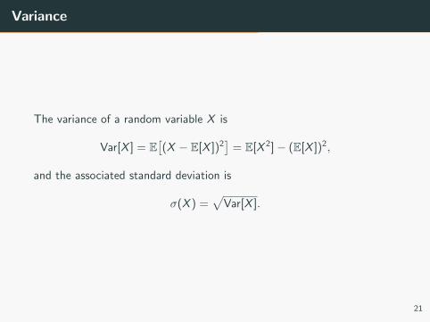
Variance
The variance of a random variable X is
Var[X ] = E[(X − E[X ])2
]= E[X 2]− (E[X ])2,
and the associated standard deviation is
σ(X ) =√
Var[X ].
21

Exercise: uniform distribution
Consider X ∼ uniform(0, 1) whose PDF is
fX (x) =
1, 0 ≤ x ≤ 1
0, otherwise
What’s the expectation and variance of X?
Hint:
• E[X ] =∫∞−∞ xfX (x)dx ;
• Var[X ] = E[X 2]− (E[X ])2.
22

Common distributions
• Normal distribution: X ∼ N (µ, σ2) has PDF
fX (x) =1√
2πσ2exp− 1
2σ2(x − µ)2.
• E[X ] = µ and Var[X ] = σ2.
• Bernoulli distribution: X ∼ Bernoulli(p) with 0 ≤ p ≤ 1 has PMF
PX (x) =
p, x = 1
1− p, x = 0
• E[X ] = p and Var[X ] = p(1− p).
23

Joint distributions
• For two random variables X and Y , their joint cumulative
distribution function is
FX ,Y (x , y) = P(X ≤ x ,Y ≤ y).
• For two discrete random variables X and Y , their joint probability
mass function is
pX ,Y (x , y) = P(X = x ,Y = y).
• For two continuous random variable X and Y , their joint probability
density function is
fX ,Y (x , y) =∂2FX ,Y (x , y)
∂x∂y,
so that for a set A ∈ R2 and a function g : R2 → R,
P((X ,Y ) ∈ A) =
∫∫(x,y)∈A
fX ,Y (x , y)dxdy ,
E[g(X ,Y )] =
∫∫g(x , y)fX ,Y (x , y)dxdy .
24

Independence
• Random variables X ,Y are independent if for any possible values
x , y
fX ,Y (x , y) = fX (x)fY (y), for continuous X ,Y ,
or pX ,Y (x , y) = pX (x)pY (y), for discrete X ,Y .
• For any set A = (x , y) : x ∈ A1, y ∈ A2 ⊂ R2, independent
random variables X ,Y satisfy that
P((X ,Y ) ∈ A) = P(X ∈ A1)P(Y ∈ A2).
or events w : X (w) ∈ A1 and w : Y (w) ∈ A2 are independent
events for any A1 and A2.
25

Exercise: Independence
For example, consider toss two coins consecutively, and X1 = 1 if the first
coin heads up, otherwise X1 = 0; X2 = 1 if the second coin heads up,
otherwise X2 = 0.
• Ω = (T ,T ), (H,H), (T ,H), (H,T ).• P(X1 = 1,X2 = 1) = P((H,H)) = 1
4 ;
• P(X1 = 1) = P((H,T ), (H,H)) = 12 ;
• P(X2 = 1) = P((T ,H), (H,H)) = 12 .
Thus
P(X1 = 1,X2 = 1) =1
4=
1
2× 1
2= P(X1 = 1)P(X2 = 1)..
Similarly, we can show that
P(X1 = 1,X2 = 0) = P(X1 = 1)P(X2 = 0)
P(X1 = 0,X2 = 1) = P(X1 = 0)P(X2 = 1)
P(X1 = 0,X2 = 0) = P(X1 = 0)P(X2 = 0).
26

Conditional Probability
Let A,B be two events.
• The conditional probability of A given B is defined as:
P(A|B) =P(A ∩ B)
P(B).
• If A is independent of B, we have P(A|B) = P(A), as
P(A | B) =P(A ∩ B)
P(B)=
P(A)P(B)
P(B)= P(A).
• Bayes Rule:
P(A|B) =P(B|A)P(A)
P(B).
• Chain Rule:
P(A1 ∩ A2 ∩ · · · ∩ An)
= P(A1)P(A2|A1)P(A3|A2 ∩ A1) . . .P(An|An−1 ∩ · · · ∩ A1).
27

Example: conditional probability
Consider toss a die once, and we define events
A = The value is larger than 4,B = The value is larger than 2.
Then
P(A | B) =P(A ∩ B)
P(B)
=P(5, 6 ∩ 3, 4, 5, 6)
P(3, 4, 5, 6)
=2646
=1
2.
28

Conditional Distribution
Conditional Density. The conditional probability density function of
continuous random variable X given Y = y is
fX (x |Y = y) =fX ,Y (x , y)
fY (y).
Conditional Expectation. The conditional expectation of X given
Y = y is
E(X |Y = y) =
∫ ∞−∞
xfX (x |Y = y)dx , g(y)
Conditional Variance. The conditional variance of random variable X
given Y = y is
Var[X |Y = y ] = E[(X − E(X |Y = y))2|Y = y ] , h(y).
Both E[X | Y ] and Var(X |Y ) are random variables, and their
distributions are determined by the distribution of Y .
29

Properties of Conditional Distributions
Iterated Expectation. Recall that E(X |Y ) is a function of Y , i.e., a
random variable. The law of iterative expectation states that
E[E(X |Y )] = E(X ).
Law of Total Variance. Recall that E(X |Y ) and Var(X |Y ) are both
random variables that are functions of Y . We have
Var(Y ) = E[Var(X |Y )] + Var [E(X |Y )].
30

Example: conditional distribution
Assume we throw two six-sided dice.
• What is the probability that the total of two dice will be greater
than 8 given that the first die is a 6?
• What is the expectation of the total of two dice given that the first
die is a 6?
• What is the variance of the total of two dice given that the first die
is a 6?
31

Example: conditional distribution
We use X1 to denote the value for the first die and X2 the value for the
second die.
• What is the probability that the total of two dice will be greater
than 8 given that the first die is a 6?
P(X1 + X2 > 8 | X1 = 6) =P(X1 + X2 > 8,X1 = 6)
P(X1 = 6)
=P(X1 = 6,X2 > 2)
P(X1 = 6)
=P(X1 = 6)P(X2 > 2)
P(X1 = 6)
= P(X2 > 2) =4
6.
32

Example: conditional distribution
• What is the expectation of the total of two dice given that the first
die is a 6?
Given that X1 = 6, X1 + X2 can be 7, 8, 9, 10, 11, 12, all with
probability 16 . Thus
E[X1 + X2 | X1 = 6] = 7 ∗ 1
6+ · · ·+ 12 ∗ 1
6=
57
6.
• What is the variance of the total of two dice given that the first die
is a 6? Answer: 10536 .
33

Law of large number
Consider i.i.d random variables X1, · · · ,Xn, i.e., independent random
variables with identical distributions, and an arbitrary function g .
Suppose the common expectation E[g(X1)] <∞ and common variance
Var[g(X1)] <∞,
limn→∞
1
n
n∑i=1
g(Xi ) = E[g(X1)].
Actually
• E[ 1n∑n
i=1 g(Xi )] = E[g(X1)].
• Var[ 1n∑n
i=1 g(Xi )] = 1n Var[g(X )].
34

Resources

Resources
• Linear algebra:
http://cs229.stanford.edu/summer2019/cs229-linalg.pdf
• Matrix calculus: https:
//www.math.uwaterloo.ca/~hwolkowi/matrixcookbook.pdf
• Probability:
http://cs229.stanford.edu/summer2019/cs229-prob.pdf and
All of Statistics by Larry Wasserman.
35