DRAFT V2.1

From

Math, Numerics, & Programming

(for Mechanical Engineers)

Masayuki Yano

James Douglass Penn

George Konidaris

Anthony T Patera

August 2013

©MIT 2011, 2012, 2013

© The Authors. License: Creative Commons Attribution-Noncommercial-Share Alike 3.0(CC BY-NC-SA 3.0), which permits unrestricted use,distribution, and reproductionin any medium, provided the original authors and MIT OpenCourseWare sourceare credited; the use isnon-commercial; and the CC BY-NC-SA license isretained. See also http://ocw.mit.edu/terms/.

Contents

I (Numerical) Calculus. Elementary Programming Concepts. 11

1 Motivation 131.1 A Mobile Robot . . . . . . . . . . . . . . . . . . . . . . . . . . . . . . . . . . . . . . 131.2 Global Position Estimation: Infra-red Range-Finding . . . . . . . . . . . . . . . . . . 131.3 Local Position Tracking: Odometry . . . . . . . . . . . . . . . . . . . . . . . . . . . . 131.4 The Numerical Tasks . . . . . . . . . . . . . . . . . . . . . . . . . . . . . . . . . . . . 16

2 Interpolation 172.1 Interpolation of Univariate Functions . . . . . . . . . . . . . . . . . . . . . . . . . . 17

2.1.1 Best Fit vs. Interpolation: Polynomials of Degree n . . . . . . . . . . . . . . 322.2 Interpolation of Bivariate Functions . . . . . . . . . . . . . . . . . . . . . . . . . . . 35

3 Differentiation 413.1 Differentiation of Univariate Functions . . . . . . . . . . . . . . . . . . . . . . . . . . 41

3.1.1 Second Derivatives . . . . . . . . . . . . . . . . . . . . . . . . . . . . . . . . . 483.2 Differentiation of Bivariate Functions . . . . . . . . . . . . . . . . . . . . . . . . . . . 50

4 Elements of a Program and Matlab Basics 534.1 Computer Architecture and Computer Programming . . . . . . . . . . . . . . . . . . 53

4.1.1 Virtual Processor . . . . . . . . . . . . . . . . . . . . . . . . . . . . . . . . . . 534.1.2 The Matlab Environment . . . . . . . . . . . . . . . . . . . . . . . . . . . . 55

4.2 Data Types (and Classes) . . . . . . . . . . . . . . . . . . . . . . . . . . . . . . . . . 554.3 Variables and Assignment . . . . . . . . . . . . . . . . . . . . . . . . . . . . . . . . . 574.4 The Workspace and Saving/Loading Data . . . . . . . . . . . . . . . . . . . . . . . . 584.5 Arithmetic Operations . . . . . . . . . . . . . . . . . . . . . . . . . . . . . . . . . . . 594.6 Floating Point Numbers (FPNs): Representation and Operations . . . . . . . . . . . 61

4.6.1 FPN Truncation and Representation . . . . . . . . . . . . . . . . . . . . . . . 614.6.2 Arithmetic Operations . . . . . . . . . . . . . . . . . . . . . . . . . . . . . . . 62

4.7 Relational and Logical Operations . . . . . . . . . . . . . . . . . . . . . . . . . . . . 654.7.1 Relational Operations . . . . . . . . . . . . . . . . . . . . . . . . . . . . . . . 654.7.2 Logical Operations . . . . . . . . . . . . . . . . . . . . . . . . . . . . . . . . . 65

4.8 Flow Control . . . . . . . . . . . . . . . . . . . . . . . . . . . . . . . . . . . . . . . . 664.8.1 The if Statement . . . . . . . . . . . . . . . . . . . . . . . . . . . . . . . . . 664.8.2 The while Statement . . . . . . . . . . . . . . . . . . . . . . . . . . . . . . . 674.8.3 The for Statement . . . . . . . . . . . . . . . . . . . . . . . . . . . . . . . . . 68

3

5 Matlab Arrays 715.1 Single-Index Floating Point Arrays . . . . . . . . . . . . . . . . . . . . . . . . . . . . 71

5.1.1 The Concept . . . . . . . . . . . . . . . . . . . . . . . . . . . . . . . . . . . . 715.1.2 Assignment and Access . . . . . . . . . . . . . . . . . . . . . . . . . . . . . . 725.1.3 (Dotted) Arithmetic Operations . . . . . . . . . . . . . . . . . . . . . . . . . 755.1.4 Relational and Logical (Array) Operations . . . . . . . . . . . . . . . . . . . . 785.1.5 “Data” Operations . . . . . . . . . . . . . . . . . . . . . . . . . . . . . . . . . 79

5.2 Characters and Character Single-Index Arrays (Strings) . . . . . . . . . . . . . . . . 835.3 Double-Index Arrays . . . . . . . . . . . . . . . . . . . . . . . . . . . . . . . . . . . . 85

5.3.1 Concept . . . . . . . . . . . . . . . . . . . . . . . . . . . . . . . . . . . . . . . 855.3.2 Assignment and Access . . . . . . . . . . . . . . . . . . . . . . . . . . . . . . 865.3.3 Operations . . . . . . . . . . . . . . . . . . . . . . . . . . . . . . . . . . . . . 92

5.4 Line Plotting . . . . . . . . . . . . . . . . . . . . . . . . . . . . . . . . . . . . . . . . 95

6 Functions in Matlab 996.1 The Advantage: Encapsulation and Re-Use . . . . . . . . . . . . . . . . . . . . . . . 996.2 Always Test a Function . . . . . . . . . . . . . . . . . . . . . . . . . . . . . . . . . . 996.3 What Happens in a Function Stays in a Function . . . . . . . . . . . . . . . . . . . . 1006.4 Syntax: Inputs (Parameters) and Outputs . . . . . . . . . . . . . . . . . . . . . . . . 1016.5 Functions of Functions: Handles . . . . . . . . . . . . . . . . . . . . . . . . . . . . . 1036.6 Anonymous (or In-Line) Functions . . . . . . . . . . . . . . . . . . . . . . . . . . . . 1046.7 String Inputs and the eval Function . . . . . . . . . . . . . . . . . . . . . . . . . . . 105

7 Integration 1077.1 Integration of Univariate Functions . . . . . . . . . . . . . . . . . . . . . . . . . . . . 1077.2 Integration of Bivariate Functions . . . . . . . . . . . . . . . . . . . . . . . . . . . . . 117

II Monte Carlo Methods. 121

8 Introduction 1238.1 Statistical Estimation and Simulation . . . . . . . . . . . . . . . . . . . . . . . . . . 123

8.1.1 Random Models and Phenomena . . . . . . . . . . . . . . . . . . . . . . . . . 1238.1.2 Statistical Estimation of Parameters/Properties of Probability Distributions . 1248.1.3 Monte Carlo Simulation . . . . . . . . . . . . . . . . . . . . . . . . . . . . . . 125

8.2 Motivation: An Example . . . . . . . . . . . . . . . . . . . . . . . . . . . . . . . . . . 126

9 Introduction to Random Variables 1299.1 Discrete Random Variables . . . . . . . . . . . . . . . . . . . . . . . . . . . . . . . . 129

9.1.1 Probability Mass Functions . . . . . . . . . . . . . . . . . . . . . . . . . . . . 1299.1.2 Transformation . . . . . . . . . . . . . . . . . . . . . . . . . . . . . . . . . . . 136

9.2 Discrete Bivariate Random Variables (Random Vectors) . . . . . . . . . . . . . . . . 1399.2.1 Joint Distributions . . . . . . . . . . . . . . . . . . . . . . . . . . . . . . . . . 1399.2.2 Characterization of Joint Distributions . . . . . . . . . . . . . . . . . . . . . . 140

9.3 Binomial Distribution . . . . . . . . . . . . . . . . . . . . . . . . . . . . . . . . . . . 1479.4 Continuous Random Variables . . . . . . . . . . . . . . . . . . . . . . . . . . . . . . . 152

9.4.1 Probability Density Function; Cumulative Distribution Function . . . . . . . 1529.4.2 Transformations of Continuous Random Variables . . . . . . . . . . . . . . . 1579.4.3 The Central Limit Theorem . . . . . . . . . . . . . . . . . . . . . . . . . . . . 1609.4.4 Generation of Pseudo-Random Numbers . . . . . . . . . . . . . . . . . . . . . 161

4

9.5 Continuous Random Vectors . . . . . . . . . . . . . . . . . . . . . . . . . . . . . . . . 163

10 Statistical Estimation: Bernoulli (Coins) 17310.1 Introduction . . . . . . . . . . . . . . . . . . . . . . . . . . . . . . . . . . . . . . . . . 17310.2 The Sample Mean: An Estimator / Estimate . . . . . . . . . . . . . . . . . . . . . . 17310.3 Confidence Intervals . . . . . . . . . . . . . . . . . . . . . . . . . . . . . . . . . . . . 177

10.3.1 Definition . . . . . . . . . . . . . . . . . . . . . . . . . . . . . . . . . . . . . . 17710.3.2 Frequentist Interpretation . . . . . . . . . . . . . . . . . . . . . . . . . . . . . 17810.3.3 Convergence . . . . . . . . . . . . . . . . . . . . . . . . . . . . . . . . . . . . 180

10.4 Cumulative Sample Means . . . . . . . . . . . . . . . . . . . . . . . . . . . . . . . . 180

11 Statistical Estimation: the Normal Density 183

12 Monte Carlo: Areas and Volumes 18712.1 Calculating an Area . . . . . . . . . . . . . . . . . . . . . . . . . . . . . . . . . . . . 187

12.1.1 Objective . . . . . . . . . . . . . . . . . . . . . . . . . . . . . . . . . . . . . . 18712.1.2 A Continuous Uniform Random Variable . . . . . . . . . . . . . . . . . . . . 18712.1.3 A Bernoulli Random Variable . . . . . . . . . . . . . . . . . . . . . . . . . . . 18812.1.4 Estimation: Monte Carlo . . . . . . . . . . . . . . . . . . . . . . . . . . . . . 18812.1.5 Estimation: Riemann Sum . . . . . . . . . . . . . . . . . . . . . . . . . . . . 190

12.2 Calculation of Volumes in Higher Dimensions . . . . . . . . . . . . . . . . . . . . . . 19312.2.1 Three Dimensions . . . . . . . . . . . . . . . . . . . . . . . . . . . . . . . . . 193

Monte Carlo . . . . . . . . . . . . . . . . . . . . . . . . . . . . . . . . . . . . 194Riemann Sum . . . . . . . . . . . . . . . . . . . . . . . . . . . . . . . . . . . . 194

12.2.2 General d-Dimensions . . . . . . . . . . . . . . . . . . . . . . . . . . . . . . . 197

13 Monte Carlo: General Integration Procedures 199

14 Monte Carlo: Failure Probabilities 20114.1 Calculating a Failure Probability . . . . . . . . . . . . . . . . . . . . . . . . . . . . . 201

14.1.1 Objective . . . . . . . . . . . . . . . . . . . . . . . . . . . . . . . . . . . . . . 20114.1.2 An Integral . . . . . . . . . . . . . . . . . . . . . . . . . . . . . . . . . . . . . 20214.1.3 A Monte Carlo Approach . . . . . . . . . . . . . . . . . . . . . . . . . . . . . 202

III Linear Algebra 1: Matrices and Least Squares. Regression. 205

15 Motivation 207

16 Matrices and Vectors: Definitions and Operations 20916.1 Basic Vector and Matrix Operations . . . . . . . . . . . . . . . . . . . . . . . . . . . 209

16.1.1 Definitions . . . . . . . . . . . . . . . . . . . . . . . . . . . . . . . . . . . . . 209Transpose Operation . . . . . . . . . . . . . . . . . . . . . . . . . . . . . . . . 210

16.1.2 Vector Operations . . . . . . . . . . . . . . . . . . . . . . . . . . . . . . . . . 211Inner Product . . . . . . . . . . . . . . . . . . . . . . . . . . . . . . . . . . . . 213Norm (2-Norm) . . . . . . . . . . . . . . . . . . . . . . . . . . . . . . . . . . . 213Orthogonality . . . . . . . . . . . . . . . . . . . . . . . . . . . . . . . . . . . . 217Orthonormality . . . . . . . . . . . . . . . . . . . . . . . . . . . . . . . . . . . 218

16.1.3 Linear Combinations . . . . . . . . . . . . . . . . . . . . . . . . . . . . . . . . 218Linear Independence . . . . . . . . . . . . . . . . . . . . . . . . . . . . . . . . 219

5

Vector Spaces and Bases . . . . . . . . . . . . . . . . . . . . . . . . . . . . . . 22016.2 Matrix Operations . . . . . . . . . . . . . . . . . . . . . . . . . . . . . . . . . . . . . 223

16.2.1 Interpretation of Matrices . . . . . . . . . . . . . . . . . . . . . . . . . . . . . 22316.2.2 Matrix Operations . . . . . . . . . . . . . . . . . . . . . . . . . . . . . . . . . 224

Matrix-Matrix Product . . . . . . . . . . . . . . . . . . . . . . . . . . . . . . 22516.2.3 Interpretations of the Matrix-Vector Product . . . . . . . . . . . . . . . . . . 228

Row Interpretation . . . . . . . . . . . . . . . . . . . . . . . . . . . . . . . . . 228Column Interpretation . . . . . . . . . . . . . . . . . . . . . . . . . . . . . . . 229Left Vector-Matrix Product . . . . . . . . . . . . . . . . . . . . . . . . . . . . 229

16.2.4 Interpretations of the Matrix-Matrix Product . . . . . . . . . . . . . . . . . . 230Matrix-Matrix Product as a Series of Matrix-Vector Products . . . . . . . . . 230Matrix-Matrix Product as a Series of Left Vector-Matrix Products . . . . . . 231

16.2.5 Operation Count of Matrix-Matrix Product . . . . . . . . . . . . . . . . . . . 23116.2.6 The Inverse of a Matrix (Briefly) . . . . . . . . . . . . . . . . . . . . . . . . . 232

16.3 Special Matrices . . . . . . . . . . . . . . . . . . . . . . . . . . . . . . . . . . . . . . 23316.3.1 Diagonal Matrices . . . . . . . . . . . . . . . . . . . . . . . . . . . . . . . . . 23416.3.2 Symmetric Matrices . . . . . . . . . . . . . . . . . . . . . . . . . . . . . . . . 23416.3.3 Symmetric Positive Definite Matrices . . . . . . . . . . . . . . . . . . . . . . . 23416.3.4 Triangular Matrices . . . . . . . . . . . . . . . . . . . . . . . . . . . . . . . . 23616.3.5 Orthogonal Matrices . . . . . . . . . . . . . . . . . . . . . . . . . . . . . . . . 23616.3.6 Orthonormal Matrices . . . . . . . . . . . . . . . . . . . . . . . . . . . . . . . 238

16.4 Further Concepts in Linear Algebra . . . . . . . . . . . . . . . . . . . . . . . . . . . 23916.4.1 Column Space and Null Space . . . . . . . . . . . . . . . . . . . . . . . . . . 23916.4.2 Projectors . . . . . . . . . . . . . . . . . . . . . . . . . . . . . . . . . . . . . . 240

17 Least Squares 24317.1 Data Fitting in Absence of Noise and Bias . . . . . . . . . . . . . . . . . . . . . . . 24317.2 Overdetermined Systems . . . . . . . . . . . . . . . . . . . . . . . . . . . . . . . . . . 248

Row Interpretation . . . . . . . . . . . . . . . . . . . . . . . . . . . . . . . . . 249Column Interpretation . . . . . . . . . . . . . . . . . . . . . . . . . . . . . . . 250

17.3 Least Squares . . . . . . . . . . . . . . . . . . . . . . . . . . . . . . . . . . . . . . . . 25117.3.1 Measures of Closeness . . . . . . . . . . . . . . . . . . . . . . . . . . . . . . . 25117.3.2 Least-Squares Formulation (`2 minimization) . . . . . . . . . . . . . . . . . . 25217.3.3 Computational Considerations . . . . . . . . . . . . . . . . . . . . . . . . . . 256

QR Factorization and the Gram-Schmidt Procedure . . . . . . . . . . . . . . 25717.3.4 Interpretation of Least Squares: Projection . . . . . . . . . . . . . . . . . . . 25917.3.5 Error Bounds for Least Squares . . . . . . . . . . . . . . . . . . . . . . . . . . 261

Error Bounds with Respect to Perturbation in Data, g (constant model) . . . 261Error Bounds with Respect to Perturbation in Data, g (general) . . . . . . . 262Error Bounds with Respect to Reduction in Space, B . . . . . . . . . . . . . 267

18 Matlab Linear Algebra (Briefly) 27118.1 Matrix Multiplication (and Addition) . . . . . . . . . . . . . . . . . . . . . . . . . . 27118.2 The Matlab Inverse Function: inv . . . . . . . . . . . . . . . . . . . . . . . . . . . 27218.3 Solution of Linear Systems: Matlab Backslash . . . . . . . . . . . . . . . . . . . . . 27318.4 Solution of (Linear) Least-Squares Problems . . . . . . . . . . . . . . . . . . . . . . . 273

6

19 Regression: Statistical Inference 27519.1 Simplest Case . . . . . . . . . . . . . . . . . . . . . . . . . . . . . . . . . . . . . . . . 275

19.1.1 Friction Coefficient Determination Problem Revisited . . . . . . . . . . . . . 27519.1.2 Response Model . . . . . . . . . . . . . . . . . . . . . . . . . . . . . . . . . . 27619.1.3 Parameter Estimation . . . . . . . . . . . . . . . . . . . . . . . . . . . . . . . 27919.1.4 Confidence Intervals . . . . . . . . . . . . . . . . . . . . . . . . . . . . . . . . 281

Individual Confidence Intervals . . . . . . . . . . . . . . . . . . . . . . . . . . 282Joint Confidence Intervals . . . . . . . . . . . . . . . . . . . . . . . . . . . . . 283

19.1.5 Hypothesis Testing . . . . . . . . . . . . . . . . . . . . . . . . . . . . . . . . . 28819.1.6 Inspection of Assumptions . . . . . . . . . . . . . . . . . . . . . . . . . . . . . 289

Checking for Plausibility of the Noise Assumptions . . . . . . . . . . . . . . . 289Checking for Presence of Bias . . . . . . . . . . . . . . . . . . . . . . . . . . . 290

19.2 General Case . . . . . . . . . . . . . . . . . . . . . . . . . . . . . . . . . . . . . . . . 29119.2.1 Response Model . . . . . . . . . . . . . . . . . . . . . . . . . . . . . . . . . . 29119.2.2 Estimation . . . . . . . . . . . . . . . . . . . . . . . . . . . . . . . . . . . . . 29219.2.3 Confidence Intervals . . . . . . . . . . . . . . . . . . . . . . . . . . . . . . . . 29319.2.4 Overfitting (and Underfitting) . . . . . . . . . . . . . . . . . . . . . . . . . . 294

IV (Numerical) Differential Equations 305

20 Motivation 307

21 Initial Value Problems 31121.1 Scalar First-Order Linear ODEs . . . . . . . . . . . . . . . . . . . . . . . . . . . . . . 311

21.1.1 Model Problem . . . . . . . . . . . . . . . . . . . . . . . . . . . . . . . . . . . 31121.1.2 Analytical Solution . . . . . . . . . . . . . . . . . . . . . . . . . . . . . . . . . 312

Homogeneous Equation . . . . . . . . . . . . . . . . . . . . . . . . . . . . . . 312Constant Forcing . . . . . . . . . . . . . . . . . . . . . . . . . . . . . . . . . . 312Sinusoidal Forcing . . . . . . . . . . . . . . . . . . . . . . . . . . . . . . . . . 313

21.1.3 A First Numerical Method: Euler Backward (Implicit) . . . . . . . . . . . . . 314Discretization . . . . . . . . . . . . . . . . . . . . . . . . . . . . . . . . . . . . 315Consistency . . . . . . . . . . . . . . . . . . . . . . . . . . . . . . . . . . . . . 316Stability . . . . . . . . . . . . . . . . . . . . . . . . . . . . . . . . . . . . . . . 318Convergence: Dahlquist Equivalence Theorem . . . . . . . . . . . . . . . . . . 319Order of Accuracy . . . . . . . . . . . . . . . . . . . . . . . . . . . . . . . . . 321

21.1.4 An Explicit Scheme: Euler Forward . . . . . . . . . . . . . . . . . . . . . . . 32121.1.5 Stiff Equations: Implicit vs. Explicit . . . . . . . . . . . . . . . . . . . . . . . 32421.1.6 Unstable Equations . . . . . . . . . . . . . . . . . . . . . . . . . . . . . . . . 32621.1.7 Absolute Stability and Stability Diagrams . . . . . . . . . . . . . . . . . . . . 326

Euler Backward . . . . . . . . . . . . . . . . . . . . . . . . . . . . . . . . . . . 326Euler Forward . . . . . . . . . . . . . . . . . . . . . . . . . . . . . . . . . . . 329

21.1.8 Multistep Schemes . . . . . . . . . . . . . . . . . . . . . . . . . . . . . . . . . 329Adams-Bashforth Schemes . . . . . . . . . . . . . . . . . . . . . . . . . . . . . 332Adams-Moulton Schemes . . . . . . . . . . . . . . . . . . . . . . . . . . . . . 333Convergence of Multistep Schemes: Consistency and Stability . . . . . . . . . 335Backward Differentiation Formulas . . . . . . . . . . . . . . . . . . . . . . . . 339

21.1.9 Multistage Schemes: Runge-Kutta . . . . . . . . . . . . . . . . . . . . . . . . 34121.2 Scalar Second-Order Linear ODEs . . . . . . . . . . . . . . . . . . . . . . . . . . . . 345

7

21.2.1 Model Problem . . . . . . . . . . . . . . . . . . . . . . . . . . . . . . . . . . . 34521.2.2 Analytical Solution . . . . . . . . . . . . . . . . . . . . . . . . . . . . . . . . . 346

Homogeneous Equation: Undamped . . . . . . . . . . . . . . . . . . . . . . . 346Homogeneous Equation: Underdamped . . . . . . . . . . . . . . . . . . . . . 348Homogeneous Equation: Overdamped . . . . . . . . . . . . . . . . . . . . . . 349Sinusoidal Forcing . . . . . . . . . . . . . . . . . . . . . . . . . . . . . . . . . 350

21.3 System of Two First-Order Linear ODEs . . . . . . . . . . . . . . . . . . . . . . . . . 35121.3.1 State Space Representation of Scalar Second-Order ODEs . . . . . . . . . . . 352

Solution by Modal Expansion . . . . . . . . . . . . . . . . . . . . . . . . . . . 35321.3.2 Numerical Approximation of a System of Two ODEs . . . . . . . . . . . . . . 355

Crank-Nicolson . . . . . . . . . . . . . . . . . . . . . . . . . . . . . . . . . . . 355General Recipe . . . . . . . . . . . . . . . . . . . . . . . . . . . . . . . . . . . 356

21.4 IVPs: System of n Linear ODEs . . . . . . . . . . . . . . . . . . . . . . . . . . . . . 360

22 Boundary Value Problems 365

23 Partial Differential Equations 367

V (Numerical) Linear Algebra 2: Solution of Linear Systems 369

24 Motivation 37124.1 A Robot Arm . . . . . . . . . . . . . . . . . . . . . . . . . . . . . . . . . . . . . . . . 37124.2 Gaussian Elimination and Sparsity . . . . . . . . . . . . . . . . . . . . . . . . . . . . 37224.3 Outline . . . . . . . . . . . . . . . . . . . . . . . . . . . . . . . . . . . . . . . . . . . 373

25 Linear Systems 37525.1 Model Problem: n = 2 Spring-Mass System in Equilibrium . . . . . . . . . . . . . . 375

25.1.1 Description . . . . . . . . . . . . . . . . . . . . . . . . . . . . . . . . . . . . . 37525.1.2 SPD Property . . . . . . . . . . . . . . . . . . . . . . . . . . . . . . . . . . . . 377

25.2 Existence and Uniqueness: n = 2 . . . . . . . . . . . . . . . . . . . . . . . . . . . . . 37925.2.1 Problem Statement . . . . . . . . . . . . . . . . . . . . . . . . . . . . . . . . . 37925.2.2 Row View . . . . . . . . . . . . . . . . . . . . . . . . . . . . . . . . . . . . . . 37925.2.3 The Column View . . . . . . . . . . . . . . . . . . . . . . . . . . . . . . . . . 38125.2.4 A Tale of Two Springs . . . . . . . . . . . . . . . . . . . . . . . . . . . . . . . 383

25.3 A “Larger” Spring-Mass System: n Degrees of Freedom . . . . . . . . . . . . . . . . 38725.4 Existence and Uniqueness: General Case (Square Systems) . . . . . . . . . . . . . . 389

26 Gaussian Elimination and Back Substitution 39126.1 A 2× 2 System (n = 2) . . . . . . . . . . . . . . . . . . . . . . . . . . . . . . . . . . 39126.2 A 3× 3 System (n = 3) . . . . . . . . . . . . . . . . . . . . . . . . . . . . . . . . . . 39326.3 General n× n Systems . . . . . . . . . . . . . . . . . . . . . . . . . . . . . . . . . . . 39626.4 Gaussian Elimination and LU Factorization . . . . . . . . . . . . . . . . . . . . . . . 39826.5 Tridiagonal Systems . . . . . . . . . . . . . . . . . . . . . . . . . . . . . . . . . . . . 399

27 Gaussian Elimination: Sparse Matrices 40327.1 Banded Matrices . . . . . . . . . . . . . . . . . . . . . . . . . . . . . . . . . . . . . . 40327.2 Matrix-Vector Multiplications . . . . . . . . . . . . . . . . . . . . . . . . . . . . . . . 40527.3 Gaussian Elimination and Back Substitution . . . . . . . . . . . . . . . . . . . . . . 406

27.3.1 Gaussian Elimination . . . . . . . . . . . . . . . . . . . . . . . . . . . . . . . 406

8

Densely-Populated Banded Systems . . . . . . . . . . . . . . . . . . . . . . . 406“Outrigger” Systems: Fill-Ins . . . . . . . . . . . . . . . . . . . . . . . . . . . 407

27.3.2 Back Substitution . . . . . . . . . . . . . . . . . . . . . . . . . . . . . . . . . 409Densely-Populated Banded Systems . . . . . . . . . . . . . . . . . . . . . . . 410“Outrigger” . . . . . . . . . . . . . . . . . . . . . . . . . . . . . . . . . . . . . 410

27.4 Fill-in and Reordering . . . . . . . . . . . . . . . . . . . . . . . . . . . . . . . . . . . 41027.4.1 A Cyclic System . . . . . . . . . . . . . . . . . . . . . . . . . . . . . . . . . . 41027.4.2 Reordering . . . . . . . . . . . . . . . . . . . . . . . . . . . . . . . . . . . . . 411

27.5 The Evil Inverse . . . . . . . . . . . . . . . . . . . . . . . . . . . . . . . . . . . . . . 413

28 Sparse Matrices in Matlab 41728.1 The Matrix Vector Product . . . . . . . . . . . . . . . . . . . . . . . . . . . . . . . . 417

28.1.1 A Mental Model . . . . . . . . . . . . . . . . . . . . . . . . . . . . . . . . . . 417Storage . . . . . . . . . . . . . . . . . . . . . . . . . . . . . . . . . . . . . . . 417Operations . . . . . . . . . . . . . . . . . . . . . . . . . . . . . . . . . . . . . 418

28.1.2 Matlab Implementation . . . . . . . . . . . . . . . . . . . . . . . . . . . . . . 419Storage . . . . . . . . . . . . . . . . . . . . . . . . . . . . . . . . . . . . . . . 419Operations . . . . . . . . . . . . . . . . . . . . . . . . . . . . . . . . . . . . . 422

28.2 Sparse Gaussian Elimination . . . . . . . . . . . . . . . . . . . . . . . . . . . . . . . 423

VI Nonlinear Equations 425

29 Newton Iteration 42729.1 Introduction . . . . . . . . . . . . . . . . . . . . . . . . . . . . . . . . . . . . . . . . . 42729.2 Univariate Newton . . . . . . . . . . . . . . . . . . . . . . . . . . . . . . . . . . . . . 429

29.2.1 The Method . . . . . . . . . . . . . . . . . . . . . . . . . . . . . . . . . . . . 42929.2.2 An Example . . . . . . . . . . . . . . . . . . . . . . . . . . . . . . . . . . . . 43029.2.3 The Algorithm . . . . . . . . . . . . . . . . . . . . . . . . . . . . . . . . . . . 43129.2.4 Convergence Rate . . . . . . . . . . . . . . . . . . . . . . . . . . . . . . . . . 43229.2.5 Newton Pathologies . . . . . . . . . . . . . . . . . . . . . . . . . . . . . . . . 434

29.3 Multivariate Newton . . . . . . . . . . . . . . . . . . . . . . . . . . . . . . . . . . . . 43429.3.1 A Model Problem . . . . . . . . . . . . . . . . . . . . . . . . . . . . . . . . . 43429.3.2 The Method . . . . . . . . . . . . . . . . . . . . . . . . . . . . . . . . . . . . 43429.3.3 An Example . . . . . . . . . . . . . . . . . . . . . . . . . . . . . . . . . . . . 43729.3.4 The Algorithm . . . . . . . . . . . . . . . . . . . . . . . . . . . . . . . . . . . 43829.3.5 Comments on Multivariate Newton . . . . . . . . . . . . . . . . . . . . . . . . 439

29.4 Continuation and Homotopy . . . . . . . . . . . . . . . . . . . . . . . . . . . . . . . . 43929.4.1 Parametrized Nonlinear Problems: A Single Parameter . . . . . . . . . . . . 43929.4.2 A Simple Example . . . . . . . . . . . . . . . . . . . . . . . . . . . . . . . . . 44129.4.3 Path Following: Continuation . . . . . . . . . . . . . . . . . . . . . . . . . . . 44229.4.4 Cold Start: Homotopy . . . . . . . . . . . . . . . . . . . . . . . . . . . . . . . 44329.4.5 A General Path Approach: Many Parameters . . . . . . . . . . . . . . . . . . 443

9

10

Unit I

(Numerical) Calculus. ElementaryProgramming Concepts.

11

Chapter 1

Motivation

1.1 A Mobile Robot

Robot self-localization, or the ability of a robot to figure out where it is within its environment, isarguably the most fundamental skill for a mobile robot, such as the one shown in Figure 1.1. Wecan divide the robot self-localization problem into two parts: global position estimation and localposition tracking. Global position estimation is the robot’s ability to determine its initial positionand orientation (collectively, pose) within a known map of its environment. Local position trackingis then the ability of the robot to track changes in its pose over time. In this assignment, we willconsider two basic approaches to global position estimation and local position tracking.

1.2 Global Position Estimation: Infra-red Range-Finding

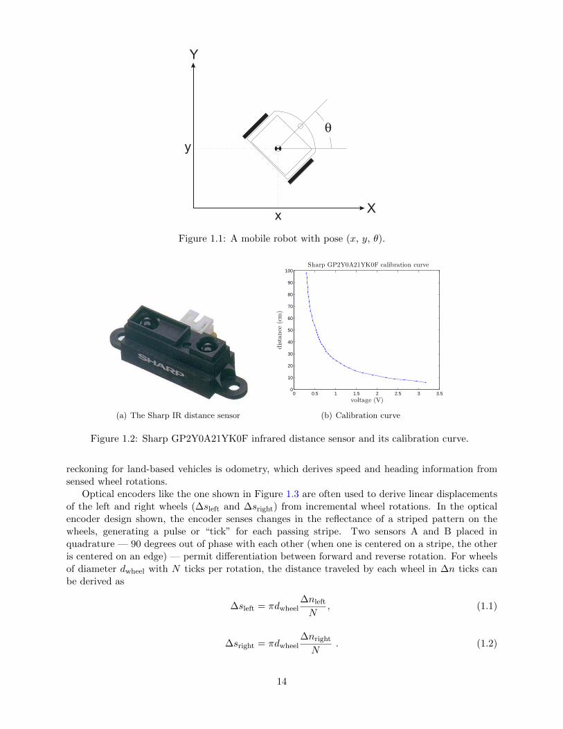
Many systems exist today for robot global position estimation. Perhaps the most familiar exampleis the Global Positioning System (GPS), a network of 24 satellites that can give an absolute po-sition estimate accurate to within several meters. For smaller scale position estimation, high-endsolutions such as robotic vision and laser range-finding can provide millimeter accuracy distancemeasurements, which can then be matched with map data to convert local distance measurementsto global position. As an alternative to these more expensive systems, ultrasonic and infrared dis-tance sensors can offer similar performance with modest compromises in speed and accuracy. Ofthese two, infrared distance sensors often have slightly narrower beam width and faster response.

Figure 1.2(a) shows the Sharp GP2Y0A21YK0F, a popular medium range (10-80 cm), infrared(IR) distance sensor. The Sharp sensor uses triangulation to calculate distance by measuring theangle of incidence of a transmitted IR beam reflected from a distant surface onto a receiving posi-tion sensitive device (PSD). Because the angle is a nonlinear function of the distance to the surface,the Sharp sensor has the nonlinear calibration curve shown in Figure 1.2(b). Given discrete cali-bration data, we can linearly interpolate voltage readings taken from the sensor to derive distancemeasurements.

1.3 Local Position Tracking: Odometry

Dead reckoning, which tracks location by integrating a moving system’s speed and heading overtime, forms the backbone of many mobile robot navigation systems. The simplest form of dead

13

DRAFT V2.1 © The Authors. License: Creative Commons BY-NC-SA 3.0.

X

Y

x

y

q

Figure 1.1: A mobile robot with pose (x, y, θ).

(a) The Sharp IR distance sensor

0 0.5 1 1.5 2 2.5 3 3.50

10

20

30

40

50

60

70

80

90

100

voltage (V)

distance

(cm)

Sharp GP2Y0A21YK0F calibration curve

(b) Calibration curve

Figure 1.2: Sharp GP2Y0A21YK0F infrared distance sensor and its calibration curve.

reckoning for land-based vehicles is odometry, which derives speed and heading information fromsensed wheel rotations.

Optical encoders like the one shown in Figure 1.3 are often used to derive linear displacementsof the left and right wheels (∆sleft and ∆sright) from incremental wheel rotations. In the opticalencoder design shown, the encoder senses changes in the reflectance of a striped pattern on thewheels, generating a pulse or “tick” for each passing stripe. Two sensors A and B placed inquadrature — 90 degrees out of phase with each other (when one is centered on a stripe, the otheris centered on an edge) — permit differentiation between forward and reverse rotation. For wheelsof diameter dwheel with N ticks per rotation, the distance traveled by each wheel in ∆n ticks canbe derived as

∆sleft = πdwheel∆nleft

N, (1.1)

∆sright = πdwheel∆nright

N. (1.2)

14

A B

Forward Reverse

A

B

Forward rotation: B lags A by 90o

A

B

Reverse rotation: A lags B by 90o

Figure 1.3: A quadrature rotary encoder and its output for clockwise and counterclockwise rotation.

dwheel 2.71 inches

Lbaseline 5.25 inches

N 60 ticks

Table 1.1: Mobile robot parameters.

By “summing up” the increments, we can compute the total cumulative distances sleft and sright

traveled by the left and right wheels, respectively.The variables time, LeftTicks, and RightTicks from assignment1.mat contain sample times

tk (in seconds) and cumulative left and right encoder counts nleft and nright, respectively, recordedduring a single test run of a mobile robot. Note that the quadrature decoding for forward andreverse rotation has already been incorporated in the data, such that cumulative counts increasefor forward rotation and decrease for reverse rotation. The values of the odometry constants forthe mobile robot are given in Table 1.

For a mobile robot with two-wheel differential drive, in which the two (left and right) drivenwheels can be controlled independently, the linear velocities vleft and vright at the two wheelsmust (assuming no slippage of the wheels) be both directed in (or opposite to) the direction θ ofthe robot’s current heading. The motion of the robot can thus be completely described by thevelocity vcenter of a point lying midway between the two wheels and the angular velocity ω aboutan instantaneous center of curvature (ICC) lying somewhere in line with the two wheels, as shownin Figure 1.4.

We can derive vcenter and ω from vleft and vright as

vcenter =vleft + vright

2, (1.3)

ω =vright − vleft

Lbaseline, (1.4)

where

vleft =dsleft

dt, (1.5)

vright =dsright

dt, (1.6)

15

qLbaseline

ICC

v right

vcenter

v left

w

Figure 1.4: Robot trajectory.

and Lbaseline is the distance between the points of contact of the two wheels. We can then integratethese velocities to track the pose [x(t), y(t), θ(t)] of the robot over time as

x(t) =

∫ t

0vcenter(t) cos[θ(t)] dt , (1.7)

y(t) =

∫ t

0vcenter(t) sin[θ(t)] dt , (1.8)

θ(t) =

∫ t

0ω(t) dt . (1.9)

In terms of the sample times tk, we can write these equations as

xk = xk−1 +

∫ tk

tk−1

vcenter(t) cos[θ(t)] dt , (1.10)

yk = yk−1 +

∫ tk

tk−1

vcenter(t) sin[θ(t)] dt , (1.11)

θk = θk−1 +

∫ tk

tk−1

ω(t) dt . (1.12)

1.4 The Numerical Tasks

To calculate distance from our transducer we must be able to interpolate; and to calculate ourposition from dead reckoning we must be able to differentiate and integrate. In this unit weintroduce the necessary numerical approaches and also understand the possible sources of error.

16

Chapter 2

Interpolation

2.1 Interpolation of Univariate Functions

The objective of interpolation is to approximate the behavior of a true underlying function usingfunction values at a limited number of points. Interpolation serves two important, distinct purposesthroughout this book. First, it is a mathematical tool that facilitates development and analysisof numerical techniques for, for example, integrating functions and solving differential equations.Second, interpolation can be used to estimate or infer the function behavior based on the functionvalues recorded as a table, for example collected in an experiment (i.e., table lookup).

Let us define the interpolation problem for an univariate function, i.e., a function of singlevariable. We discretize the domain [x1, xN ] into N − 1 non-overlapping segments, {S1, . . . , SN−1},using N points, {x1, . . . , xN}, as shown in Figure 2.1. Each segment is defined by

Si = [xi, xi+1], i = 1, . . . , N − 1 ,

and we denote the length of the segment by h, i.e.

h ≡ xi+1 − xi .

For simplicity, we assume h is constant throughout the domain. Discretization is a concept thatis used throughout numerical analysis to approximate a continuous system (infinite-dimensionalproblem) as a discrete system (finite-dimensional problem) so that the solution can be estimatedusing a computer. For interpolation, discretization is characterized by the segment size h; smallerh is generally more accurate but more costly.

Suppose, on segment Si, we are given M interpolation points

xm, m = 1, . . . ,M ,

x1

x2

x3

x4

S1

S2

S3

hx

N−1x

N

SN−1

Figure 2.1: Discretization of a 1-D domain into N − 1 segments.

17

DRAFT V2.1 © The Authors. License: Creative Commons BY-NC-SA 3.0.

x1

x2

x3

x4

x5

S2

discretization

x1 x2 x3

local segment S2

x1

x2

x3

x4

x5

x6

x7

x8

x9

function evaluation points

(a) discretization

ei

S i

(x1 , f(x1))

(x2 , f(x2))

(x3 , f(x3))

xi xi+1

interpolant

interpolation points

function

(b) local interpolation

Figure 2.2: Example of a 1-D domain discretized into four segments, a local segment with M = 3function evaluation points (i.e., interpolation points), and global function evaluation points (left).Construction of an interpolant on a segment (right).

and the associated function values

f(xm), m = 1, . . . ,M .

We wish to approximate f(x) for any given x in Si. Specifically, we wish to construct an interpolantIf that approximates f in the sense that

(If)(x) ≈ f(x), ∀ x ∈ Si ,

and satisfies

(If)(xm) = f(xm), m = 1, . . . ,M .

Note that, by definition, the interpolant matches the function value at the interpolation points,{xm}.

The relationship between the discretization, a local segment, and interpolation points is illus-trated in Figure 2.2(a). The domain [x1, x5] is discretized into four segments, delineated by thepoints xi, i = 1, . . . , 5. For instance, the segment S2 is defined by x2 and x3 and has a characteristiclength h = x3−x2. Figure 2.2(b) illustrates construction of an interpolant on the segment S2 usingM = 3 interpolation points. Note that we only use the knowledge of the function evaluated at theinterpolation points to construct the interpolant. In general, the points delineating the segments,xi, need not be function evaluation points xi, as we will see shortly.

We can also use the interpolation technique in the context of table lookup, where a table consistsof function values evaluated at a set of points, i.e., (xi, f(xi)). Given a point of interest x, we firstfind the segment in which the point resides, by identifying Si = [xi, xi+1] with xi ≤ x ≤ xi+1.Then, we identify on the segment Si the evaluation pairs (xj , f(xj)), j = . . ., ⇒ (xm, f(xm)),m = 1, . . . ,M . Finally, we calculate the interpolant at x to obtain an approximation to f(x),(If)(x).

(Note that, while we use fixed, non-overlapping segments to construct our interpolant in thischapter, we can be more flexible in the choice of segments in general. For example, to estimate

18

the value of a function at some point x, we can choose a set of M data points in the neighborhoodof x. Using the M points, we construct a local interpolant as in Figure 2.2(b) and infer f(x)by evaluating the interpolant at x. Note that the local interpolant constructed in this mannerimplicitly defines a local segment. The segment “slides” with the target x, i.e., it is adaptivelychosen. In the current chapter on interpolation and in Chapter 7 on integration, we will emphasizethe fixed segment perspective; however, in discussing differentiation in Chapter 3, we will adoptthe sliding segment perspective.)

To assess the quality of the interpolant, we define its error as the maximum difference betweenthe true function and the interpolant in the segment, i.e.

ei ≡ maxx∈Si|f(x)− (If)(x)| .

Because the construction of an interpolant on a given segment is independent of that on anothersegment1, we can analyze the local interpolation error one segment at a time. The locality ofinterpolation construction and error greatly simplifies the error analysis. In addition, we definethe maximum interpolation error, emax, as the maximum error over the entire domain, which isequivalent to the largest of the segment errors, i.e.

emax ≡ maxi=1,...,N−1

ei .

The interpolation error is a measure we use to assess the quality of different interpolation schemes.Specifically, for each interpolation scheme, we bound the error in terms of the function f and thediscretization parameter h to understand how the error changes as the discretization is refined.

Let us consider an example of interpolant.

Example 2.1.1 piecewise-constant, left endpointThe first example we consider uses a piecewise-constant polynomial to approximate the functionf . Because a constant polynomial is parameterized by a single value, this scheme requires oneinterpolation point per interval, meaning M = 1. On each segment Si = [xi, xi+1], we choose theleft endpoint as our interpolation point, i.e.

x1 = xi .

As shown in Figure 2.3, we can also easily associate the segmentation points, xi, with the globalfunction evaluation points, xi, i.e.

xi = xi, i = 1, . . . , N − 1 .

Extending the left-endpoint value to the rest of the segment, we obtain the interpolant of the form

(If)(x) = f(x1) = f(xi) = f(xi), ∀ x ∈ Si .

Figure 2.4(a) shows the interpolation scheme applied to f(x) = exp(x) over [0, 1] with N =5. Because f ′ > 0 over each interval, the interpolant If always underestimate the value of f .Conversely, if f ′ < 0 over an interval, the interpolant overestimates the values of f in the interval.The interpolant is exact over the interval if f is constant.

If f ′ exists, the error in the interpolant is bounded by

ei ≤ h ·maxx∈Si|f ′(x)| .

1for the interpolants considered in this chapter

19

x1

x2

x3

x4

x5

S2

discretization

x1

local segment S2

x1

x2

x3

x4

function evaluation points

Figure 2.3: The relationship between the discretization, a local segment, and the function evaluationpoints for a piecewise-constant, left-endpoint interpolant.

0 0.2 0.4 0.6 0.8 10.5

1

1.5

2

2.5

3

interpolant

interpolation points

function

(a) interpolant

1 2 4 8 16 3210

−2

10−1

100

101

−1.00

1/h

ma

x(e

i)

(b) error

Figure 2.4: Piecewise-constant, left-endpoint interpolant.

20

Since ei = O(h) and the error scales as the first power of h, the scheme is said to be first-orderaccurate. The convergence behavior of the interpolant applied to the exponential function is shownin Figure 2.4(b), where the maximum value of the interpolation error, emax = maxi ei, is plotted asa function of the number of intervals, 1/h.

We pause to review two related concepts that characterize asymptotic behavior of a sequence:the big-O notation (O( · )) and the asymptotic notation (∼). Say that Q and z are scalar quantities(real numbers) and q is a function of z. Using the big-O notation, when we say that Q is O(q(z))as z tends to, say, zero (or infinity), we mean that there exist constants C1 and z∗ such that|Q| < C1|q(z)|, ∀ z < z∗ (or ∀ z > z∗). On the other hand, using the asymptotic notation, whenwe say that Q ∼ C2q(z) as z tends to some limit, we mean that there exist a constant C2 (notnecessary equal to C1) such that Q/(C2q(z)) tends to unity as z tends to the limit. We shall usethese notations in two cases in particular: (i) when z is δ, a discretization parameter (h in ourexample above) — which tends to zero; (ii) when z is K, an integer related to the number of degreesof freedom that define a problem (N in our example above) — which tends to infinity. Note weneed not worry about small effects with the O (or the asymptotic) notation: for K tends to infinity,for example, O(K) = O(K − 1) = O(K +

√K). Finally, we note that the expression Q = O(1)

means that Q effectively does not depend on some (implicit, or “understood”) parameter, z.2

If f(x) is linear, then the error bound can be shown using a direct argument. Let f(x) = mx+b.The difference between the function and the interpolant over Si is

f(x)− (If)(x) = [mx− b]− [mx1 − b] = m · (x− x1) .

Recalling the local error is the maximum difference in the function and interpolant and noting thatSi = [xi, xi+1] = [x1, x1 + h], we obtain

ei = maxx∈Si

|f(x)− (If)(x)| = maxx∈Si

|m · (x− x1)| = |m| · maxx∈[x1,x1+h]

|x− x1| = |m| · h .

Finally, recalling that m = f ′(x) for the linear function, we have ei = |f ′(x)| · h. Now, let us provethe error bound for a general f .

Proof. The proof follows from the definition of the interpolant and the fundamental theorem ofcalculus, i.e.

f(x)− (If)(x) = f(x)− f(x1) (by definition of (If))

=

∫ x

x1f ′(ξ)dξ (fundamental theorem of calculus)

≤∫ x

x1|f ′(ξ)|dξ

≤ maxx∈[x1,x]

|f ′(x)|∣∣∣∣∫ x

x1dξ

∣∣∣∣ (Holder’s inequality)

≤ maxx∈Si|f ′(x)| · h, ∀ x ∈ Si = [x1, x1 + h] .

Substitution of the expression into the definition of the error yields

ei ≡ maxx∈Si|f(x)− (If)(x)| ≤ max

x∈Si|f ′(x)| · h .

2The engineering notation Q = O(103) is somewhat different and really just means that the number is roughly103.

21

0 0.2 0.4 0.6 0.8 1

0

0.2

0.4

0.6

0.8

1

interpolantinterpolation pointsfunction

(a) interpolant

1 2 4 8 16 3210

−2

10−1

100

101

1/h

ma

x(e

i)

(b) error

Figure 2.5: Piecewise-constant, left-endpoint interpolant for a non-smooth function.

It is important to note that the proof relies on the smoothness of f . In fact, if f is discontinuousand f ′ does not exist, then ei can be O(1). In other words, the interpolant does not converge tothe function (in the sense of maximum error), even if the h is refined. To demonstrate this, let usconsider a function

f(x) =

sin(πx), x ≤ 1

31

2sin(πx), x >

1

3

,

which is discontinuous at x = 1/3. The result of applying the piecewise constant, left-endpointrule to the function is shown in Figure 2.5(a). We note that the solution on the third segment isnot approximated well due to the presence of the discontinuity. More importantly, the convergenceplot, Figure 2.5(b), confirms that the maximum interpolation error does not converge even if his refined. This reduction in the convergence rate for non-smooth functions is not unique to thisparticular interpolation rule; all interpolation rules suffer from this problem. Thus, we must becareful when we interpolate a non-smooth function.

Finally, we comment on the distinction between the “best fit” (in some norm, or metric) andthe interpolant. The best fit in the “max” or “sup” norm of a constant function ci to f(x) overSi minimizes |ci − f(x)| over Si and will typically be different and perforce better (in the chosennorm) than the interpolant. However, the determination of ci in principle requires knowledge off(x) at (almost) all points in Si whereas the interpolant only requires knowledge of f(x) at onepoint — hence much more useful. We discuss this further in Section 2.1.1.

·Let us more formally define some of the key concepts visited in the first example. While we

introduce the following concepts in the context of analyzing the interpolation schemes, the conceptsapply more generally to analyzing various numerical schemes.

• Accuracy relates how well the numerical scheme (finite-dimensional) approximates the con-tinuous system (infinite-dimensional). In the context of interpolation, the accuracy tells howwell the interpolant If approximates f and is measured by the interpolation error, emax.

22

• Convergence is the property that the error vanishes as the discretization is refined, i.e.

emax → 0 as h→ 0 .

A convergent scheme can achieve any desired accuracy (error) in infinite prediction arith-metics by choosing h sufficiently small. The piecewise-constant, left-endpoint interpolant isa convergent scheme, because emax = O(h), and emax → 0 as h→ 0.

• Convergence rate is the power p such that

emax ≤ Chp as h→ 0 ,

where C is a constant independent of h. The scheme is first-order accurate for p = 1, second-order accurate for p = 2, and so on. The piecewise-constant, left-endpoint interpolant isfirst-order accurate because emax = Ch1. Note here p is fixed and the convergence (withnumber of intervals) is thus algebraic.

Note that typically as h→ 0 we obtain not a bound but in fact asymptotic behavior: emax ∼Chp or equivalently, emax/(Ch

p) → 1, as h → 0. Taking the logarithm of emax ∼ Chp,we obtain ln(emax) ∼ lnC + p lnh. Thus, a log-log plot is a convenient means of finding pempirically.

• Resolution is the characteristic length hcrit for any particular problem (described by f) forwhich we see the asymptotic convergence rate for h ≤ hcrit. Convergence plot in Figure 2.4(b)shows that the piecewise-constant, left-endpoint interpolant achieves the asymptotic conver-gence rate of 1 with respect to h for h ≤ 1/2; note that the slope from h = 1 to h = 1/2is lower than unity. Thus, hcrit for the interpolation scheme applied to f(x) = exp(x) isapproximately 1/2.

• Computational cost or operation count is the number of floating point operations (FLOPs3) tocompute Ih. As h→ 0, the number of FLOPs approaches∞. The scaling of the computationcost with the size of the problem is referred to as computational complexity . The actual run-time of computation is a function of the computational cost and the hardware. The cost ofconstructing the piecewise-constant, left end point interpolant is proportional to the numberof segments. Thus, the cost scales linearly with N , and the scheme is said to have linearcomplexity.

• Memory or storage is the number of floating point numbers that must be stored at any pointduring execution.

We note that the above properties characterize a scheme in infinite precision representation andarithmetic. Precision is related to machine precision, floating point number truncation, roundingand arithmetic errors, etc, all of which are absent in infinite-precision arithmetics.

We also note that there are two conflicting demands; the accuracy of the scheme increaseswith decreasing h (assuming the scheme is convergent), but the computational cost increases withdecreasing h. Intuitively, this always happen because the dimension of the discrete approximationmust be increased to better approximate the continuous system. However, some schemes producelower error for the same computational cost than other schemes. The performance of a numericalscheme is assessed in terms of the accuracy it delivers for a given computational cost.

We will now visit several other interpolation schemes and characterize the schemes using theabove properties.

3Not to be confused with the FLOPS (floating point operations per second), which is often used to measure theperformance of a computational hardware.

23

0 0.2 0.4 0.6 0.8 10.5

1

1.5

2

2.5

3

interpolant

interpolation points

function

Figure 2.6: Piecewise-constant, right-endpoint interpolant.

Example 2.1.2 piecewise-constant, right end pointThis interpolant also uses a piecewise-constant polynomial to approximate the function f , and thusrequires one interpolation point per interval, i.e., M = 1. This time, the interpolation point is atthe right endpoint, instead of the left endpoint, resulting in

x1 = xi+1, (If)(x) = f(x1) = f(xi+1), ∀ x ∈ Si = [xi, xi+1] .

The global function evaluation points, xi, are related to segmentation points, xi, by

xi = xi+1, i = 1, . . . , N − 1 .

Figure 2.6 shows the interpolation applied to the exponential function.If f ′ exists, the error in the interpolant is bounded by

ei ≤ h ·maxx∈Si|f ′(x)| ,

and thus the scheme is first-order accurate. The proof is similar to that of the piecewise-constant,right-endpoint interpolant.

·

Example 2.1.3 piecewise-constant, midpointThis interpolant uses a piecewise-constant polynomial to approximate the function f , but uses themidpoint of the segment, Si = [xi, xi+1], as the interpolation point, i.e.

x1 =1

2(xi + xi+1) .

Denoting the (global) function evaluation point associated with segment Si as xi, we have

xi =1

2(xi + xi+1), i = 1, . . . , N − 1 ,

as illustrated in Figure 2.7. Note that the segmentation points xi do not correspond to the functionevaluation points xi unlike in the previous two interpolants. This choice of interpolation pointresults in the interpolant

(If)(x) = f(x1) = f(xi) = f

(1

2(xi + xi+1)

), x ∈ Si .

24

x1

x2

x3

x4

x5

S2

discretization

x1

local segment S2

x1

x2

x3

x4

function evaluation points

Figure 2.7: The relationship between the discretization, a local segment, and the function evaluationpoints for a piecewise-constant, midpoint interpolant.

Figure 2.8(a) shows the interpolant for the exponential function. In the context of table lookup,this interpolant naturally arises if a value is approximated from a table of data choosing the nearestdata point.

The error of the interpolant is bounded by

ei ≤h

2·maxx∈Si|f ′(x)| ,

where the factor of half comes from the fact that any function evaluation point is less than h/2distance away from one of the interpolation points. Figure 2.8(a) shows that the midpoint inter-polant achieves lower error than the left- or right-endpoint interpolant. However, the error stillscales linearly with h, and thus the midpoint interpolant is first-order accurate.

For a linear function f(x) = mx + b, the sharp error bound can be obtained from a directargument. The difference between the function and its midpoint interpolant is

f(x)− (If)(x) = [mx+ b]−[mx1 + b

]= m · (x− x1) .

The difference vanishes at the midpoint, and increases linearly with the distance from the midpoint.Thus, the difference is maximized at either of the endpoints. Noting that the segment can be

expressed as Si = [xi, xi+1] =[x1 − h

2 , x1 + h

2

], the maximum error is given by

ei ≡ maxx∈Si

(f(x)− (If)(x)) = maxx∈[x1−h2 ,x1+h

2 ]|m · (x− x1)|

= |m · (x− x1)|x=x1±h/2 = |m| · h2.

Recalling m = f ′(x) for the linear function, we have ei = |f ′(x)|h/2. A sharp proof for a general ffollows essentially that for the piecewise-constant, left-endpoint rule.

25

0 0.2 0.4 0.6 0.8 10.5

1

1.5

2

2.5

3

interpolant

interpolation points

function

(a) interpolant

1 2 4 8 16 3210

−2

10−1

100

101

−1.00

1/h

max(e

i)

constant, left

constant, right

constant, middle

(b) error

Figure 2.8: Piecewise-constant, mid point interpolant.

Proof. The proof follows from the fundamental theorem of calculus,

f(x)− (If)(x) = f(x)− f(x1)

=

∫ x

x1f ′(ξ)dξ ≤

∫ x

x1|f ′(ξ)|dξ ≤ max

x∈[x1,x]|f ′(x)|

∣∣∣∣∫ x

x1dξ

∣∣∣∣≤ max

x∈[x1−h2 ,x1+h2 ]|f ′(x)| · h

2, ∀ x ∈ Si =

[x1 − h

2, x1 +

h

2

].

Thus, we have

ei = maxx∈Si|f(x)− (If)(x)| ≤ max

x∈Si|f ′(x)| · h

2.

·

Example 2.1.4 piecewise-linearThe three examples we have considered so far used piecewise-constant functions to interpolate thefunction of interest, resulting in the interpolants that are first-order accurate. In order to improvethe quality of interpolation, we consider a second-order accurate interpolant in this example. Toachieve this, we choose a piecewise-linear function (i.e., first-degree polynomials) to approximate thefunction behavior. Because a linear function has two coefficients, we must choose two interpolationpoints per segment to uniquely define the interpolant, i.e., M = 2. In particular, for segmentSi = [xi, xi+1], we choose its endpoints, xi and xi+1, as the interpolation points, i.e.

x1 = xi and x2 = xi+1 .

The (global) function evaluation points and the segmentation points are trivially related by

xi = xi, i = 1, . . . , N ,

26

x1

x2

x3

x4

x5

S2

discretization

x1 x2

local segment S2

x1

x2

x3

x4

x5

function evaluation points

Figure 2.9: The relationship between the discretization, a local segment, and the function evaluationpoints for a linear interpolant.

as illustrated in Figure 2.9.The resulting interpolant, defined using the local coordinate, is of the form

(If)(x) = f(x1) +

(f(x2)− f(x1)

h

)(x− x1), ∀ x ∈ Si , (2.1)

or, in the global coordinate, is expressed as

(If)(x) = f(xi) +

(f(xi+1)− f(xi)

hi

)(x− xi), ∀ x ∈ Si .

Figure 2.10(a) shows the linear interpolant applied to f(x) = exp(x) over [0, 1] with N = 5. Notethat this interpolant is continuous across the segment endpoints, because each piecewise-linearfunction matches the true function values at its endpoints. This is in contrast to the piecewise-constant interpolants considered in the previous three examples, which were discontinuous acrossthe segment endpoints in general.

If f ′′ exists, the error of the linear interpolant is bounded by

ei ≤h2

8·maxx∈Si|f ′′(x)| .

The error of the linear interpolant converges quadratically with the interval length, h. Because theerror scales with h2, the method is said to be second-order accurate. Figure 2.10(b) shows thatthe linear interpolant is significantly more accurate than the piecewise-linear interpolant for theexponential function. This trend is generally true for sufficient smooth functions. More importantly,the higher-order convergence means that the linear interpolant approaches the true function at afaster rate than the piecewise-constant interpolant as the segment length decreases.

Let us provide a sketch of the proof. First, noting that f(x)−(If)(x) vanishes at the endpoints,we express our error as

f(x)− (If)(x) =

∫ x

x1(f − If)′(t) dt .

Next, by the Mean Value Theorem (MVT), we have a point x∗ ∈ Si = [x1, x2] such that f ′(x∗) −(If)′(x∗) = 0. Note the MVT — for a continuously differentiable function f there exists an

27

0 0.2 0.4 0.6 0.8 10.5

1

1.5

2

2.5

3

interpolant

interpolation points

function

(a) interpolant

1 2 4 8 16 3210

−4

10−3

10−2

10−1

100

101

−1.00

−2.00

1/h

max(e

i)

constant, left

linear

(b) error

Figure 2.10: Piecewise-linear interpolant.

x∗ ∈ [x1, x2] such that f ′(x∗) = (f(x2) − f(x1))/h — follows from Rolle’s Theorem. Rolle’sTheorem states that, for a continuously differentiable function g that vanishes at x1 and x2, thereexists a point x∗ for which g′(x∗) = 0. To derive the MVT we take g(x) = f(x) − If(x) for Ifgiven by Eq. (2.1). Applying the fundamental theorem of calculus again, the error can be expressedas

f(x)− (If)(x) =

∫ x

x1(f − If)′(t) dt =

∫ x

x1

∫ t

x∗(f − If)′′(s) ds dt =

∫ x

x1

∫ t

x∗f ′′(s) ds dt

≤ maxx∈Si|f ′′(x)|

∫ x

x1

∫ t

x∗ds dt ≤ h2

2·maxx∈Si|f ′′(x)| .

This simple sketch shows that the interpolation error is dependent on the second derivative of fand quadratically varies with the segment length h; however, the constant is not sharp. A sharpproof is provided below.

Proof. Our objective is to obtain a bound for |f(x) − If(x)| for an arbitrary x ∈ Si. If x is theone of the endpoints, the interpolation error vanishes trivially; thus, we assume that x is not one ofthe endpoints. The proof follows from a construction of a particular quadratic interpolant and theapplication of the Rolle’s theorem. First let us form the quadratic interpolant, q(x), of the form

q(x) ≡ (If)(x) + λw(x) with w(x) = (x− x1)(x− x2) .

Since (If) matches f at x1 and x2 and q(x1) = q(x2) = 0, q(x) matches f at x1 and x2. We selectλ such that q matches f at x, i.e.

q(x) = (If)(x) + λw(x) = f(x) ⇒ λ =f(x)− (If)(x)

w(x).

The interpolation error of the quadratic interpolant is given by

φ(x) = f(x)− q(x) .

28

Because q is the quadratic interpolant of f defined by the interpolation points x1, x2, and x, φ hasthree zeros in Si. By Rolle’s theorem, φ′ has two zeros in Si. Again, by Rolle’s theorem, φ′′ hasone zero in Si. Let this zero be denoted by ξ, i.e., φ′′(ξ) = 0. Evaluation of φ′′(ξ) yields

0 = φ′′(ξ) = f ′′(ξ)− q′′(ξ) = f ′′(ξ)− (If)′′(ξ)− λw′′(ξ) = f ′′(ξ)− 2λ ⇒ λ =1

2f ′′(ξ) .

Evaluating φ(x), we obtain

0 = φ(x) = f(x)− (If)(x)− 1

2f ′′(ξ)w(x) (2.2)

f(x)− (If)(x) =1

2f ′′(ξ)(x− x1)(x− x2) . (2.3)

The function is maximized for x∗ = (x1 + x2)/2, which yields

f(x)− (If)(x) ≤ 1

8f ′′(ξ)(x2 − x1)2 =

1

8h2f ′′(ξ), ∀ x ∈ [x1, x2]

Since ξ ∈ Si, it follows that,

ei = maxx∈Si|f(x)− (If)(x)| ≤ 1

8h2f ′′(ξ) ≤ 1

8h2 max

x∈Si|f ′′(x)| .

·

Example 2.1.5 piecewise-quadraticMotivated by the higher accuracy provided by the second-order accurate, piecewise-linear inter-polants, we now consider using a piecewise-quadratic polynomial to construct an interpolant. Be-cause a quadratic function is characterized by three parameters, we require three interpolationpoints per segment (M = 3). For segment Si = [xi, xi+1], a natural choice are the two endpointsand the midpoint, i.e.

x1 = xi, x2 =1

2(xi + xi+1), and x3 = xi+1 .

To construct the interpolant, we first construct Lagrange basis polynomial of the form

φ1(x) =(x− x2)(x− x3)

(x1 − x2)(x1 − x3), φ2(x) =

(x− x1)(x− x3)

(x2 − x1)(x2 − x3), and φ3(x) =

(x− x1)(x− x2)

(x3 − x1)(x3 − x2).

By construction, φ1 takes the value of 1 at x1 and vanishes at x2 and x3. More generally, theLagrange basis has the property

φm(xn) =

1, n = m

0, n 6= m.

Using these basis functions, we can construct the quadratic interpolant as

(If)(x) = f(x1)φ1(x) + f(x2)φ2(x) + f(x3)φ3(x), ∀ x ∈ Si . (2.4)

29

0 0.2 0.4 0.6 0.8 10.5

1

1.5

2

2.5

3

interpolant

interpolation points

function

(a) interpolant

1 2 4 8 16 3210

−8

10−6

10−4

10−2

100

102

−1.00

−2.00

−3.00

1/h

max(e

i)

constant, left

linear

quadratic

(b) error

Figure 2.11: Piecewise-quadratic interpolant.

We can easily confirm that the quadratic function goes through the interpolation points, (xm, f(xm)),m = 1, 2, 3, using the property of the Lagrange basis. Figure 2.11(a) shows the interpolant for theexponential function.

If f ′′′ exists, the error of the quadratic interpolant is bounded by

ei ≤h3

72√

3maxx∈Si

f ′′′(x) .

The error converges as the cubic power of h, meaning the scheme is third-order accurate. Fig-ure 2.11(b) confirms the higher-order convergence of the piecewise-quadratic interpolant.

Proof. The proof is an extension of that for the linear interpolant. First, we form a cubic interpolantof the form

q(x) ≡ (If)(x) + λw(x) with w(x) = (x− x1)(x− x2)(x− x3) .

We select λ such that q matches f at x. The interpolation error function,

φ(x) = f(x)− q(x) ,

has four zeros in Si, specifically x1, x2, x3, and x. By repeatedly applying the Rolle’s theoremthree times, we note that φ′′′(x) has one zero in Si. Let us denote this zero by ξ, i.e., φ′′′(ξ) = 0.This implies that

φ′′′(ξ) = f ′′′(ξ)− (cIf)′′′(ξ)− λw′′′(ξ) = f ′′′(ξ)− 6λ = 0 ⇒ λ =1

6f ′′′(ξ) .

Rearranging the expression for φ(x), we obtain

f(x)− (If)(x) =1

6f ′′′(ξ)w(x) .

30

0 0.2 0.4 0.6 0.8 1

0

0.2

0.4

0.6

0.8

1

interpolantinterpolation pointsfunction

(a) interpolant

1 2 4 8 16 3210

−2

10−1

100

101

1/h

max(e

i)

constant, left

linear

quadratic

(b) error

Figure 2.12: Piecewise-quadratic interpolant for a non-smooth function.

The maximum value that w takes over Si is h3/(12√

3). Combined with the fact f ′′′(ξ) ≤maxx∈Si f

′′′(x), we obtain the error bound

ei = maxx∈Si|f(x)− (If)(x)| ≤ h3

72√

3maxx∈Si

f ′′′(x) .

Note that the extension of this proof to higher-order interpolants is straight forward. In general, apiecewise pth-degree polynomial interpolant exhibits p+ 1 order convergence.

·The procedure for constructing the Lagrange polynomials extends to arbitrary degree polyno-

mials. Thus, in principle, we can construct an arbitrarily high-order interpolant by increasing thenumber of interpolation points. While the higher-order interpolation yielded a lower interpolationerror for the smooth function considered, a few cautions are in order.

First, higher-order interpolants are more susceptible to modeling errors. If the underlying datais noisy, the “overfitting” of the noisy data can lead to inaccurate interpolant. This will be discussedin more details in Unit III on regression.

Second, higher-order interpolants are also typically not advantageous for non-smooth functions.To see this, we revisit the simple discontinuous function,

f(x) =

sin(πx), x ≤ 1

31

2sin(πx), x >

1

3

.

The result of applying the piecewise-quadratic interpolation rule to the function is shown in Fig-ure 2.12(a). The quadratic interpolant closely matches the underlying function in the smooth region.However, in the third segment, which contains the discontinuity, the interpolant differs consider-ably from the underlying function. Similar to the piecewise-constant interpolation of the function,we again commit O(1) error measured in the maximum difference. Figure 2.12(b) confirms that

31

the higher-order interpolants do not perform any better than the piecewise-constant interpolantin the presence of discontinuity. Formally, we can show that the maximum-error convergence ofany interpolation scheme can be no better than hr, where r is the highest-order derivative thatis defined everywhere in the domain. In the presence of a discontinuity, r = 0, and we observeO(hr) = O(1) convergence (i.e., no convergence).

Third, for a very high-order polynomials, the interpolation points must be chosen carefully toachieve a good result. In particular, the uniform distribution suffers from the behavior knownas Runge’s phenomenon, where the interpolant exhibits excessive oscillation even if the underlyingfunction is smooth. The spurious oscillation can be minimized by clustering the interpolation pointsnear the segment endpoints, e.g., Chebyshev nodes.

Advanced Material

2.1.1 Best Fit vs. Interpolation: Polynomials of Degree n

We will study in more details how the choice of interpolation points affect the quality of a polynomialinterpolant. For convenience, let us denote the space of nth-degree polynomials on segment S byPn(S). For consistency, we will denote nth-degree polynomial interpolant of f , which is definedby n + 1 interpolation points {xm}n+1

m=1, by Inf . We will compare the quality of the interpolantwith the “best” n+ 1 degree polynomial. We will define “best” in the infinity norm, i.e., the bestpolynomial v∗ ∈ Pn(S) satisfies

maxx∈S|f(x)− v∗(x)| ≤ max

x∈S|f(x)− v(x)| , ∀ v ∈ Pn(x) .

In some sense, the polynomial v∗ fits the function f as closely as possible. Then, the quality ofa nth-degree interpolant can be assessed by measuring how close it is to v∗. More precisely, wequantify its quality by comparing the maximum error of the interpolant with that of the bestpolynomial, i.e.

maxx∈S|f(x)− (If)(x)| ≤ (1 + Λ({xm}n+1

m=1)) maxx∈S|f(x)− v∗(x)| ,

where the constant Λ is called the Lebesgue constant. Clearly, a smaller Lebesgue constant impliessmaller error, so higher the quality of the interpolant. At the same time, Λ ≥ 0 because themaximum error in the interpolant cannot be better than that of the “best” function, which bydefinition minimizes the maximum error. In fact, the Lebesgue constant is given by

Λ({xm}n+1

m=1

)= max

x∈S

n+1∑m=1

|φm(x)| ,

where φm, m = 1, . . . , n+ 1, are the Lagrange bases functions defined by the nodes {xm}n+1m=1.

Proof. We first express the interpolation error in the infinity norm as the sum of two contributions

maxx∈S|f(x)− (If)(x)| ≤ max

x∈S|f(x)− v∗(x) + v∗(x)− (If)(x)|

≤ maxx∈S|f(x)− v∗(x)|+ max

x∈S|v∗(x)− (If)(x)|.

32

Noting that the functions in the second term are polynomial, we express them in terms of theLagrange basis φm, m = 1, . . . , n,

maxx∈S|v∗(x)− (If)(x)| = max

x∈S

∣∣∣∣∣∣n+1∑m=1

(v∗(xm)− (If)(xm))φm(x)

∣∣∣∣∣∣≤ max

x∈S

∣∣∣∣∣∣ maxm=1,...,n+1

|v∗(xm)− (If)(xm)| ·n+1∑m=1

|φm(x)|

∣∣∣∣∣∣= max

m=1,...,n+1|v∗(xm)− (If)(xm)| ·max

x∈S

n+1∑m=1

|φm(x)| .

Because If is an interpolant, we have f(xm) = (If)(xm), m = 1, . . . , n+1. Moreover, we recognizethat the second term is the expression for Lebesgue constant. Thus, we have

maxx∈S|v∗(x)− (If)(x)| ≤ max

m=1,...,n+1|v∗(xm)− f(xm)| · Λ

≤ maxx∈S|v∗(x)− f(x)|Λ .

where the last inequality follows from recognizing xm ∈ S, m = 1, . . . , n+1. Thus, the interpolationerror in the maximum norm is bounded by

maxx∈S|f(x)− (If)(x)| ≤ max

x∈S|v∗(x)− f(x)|+ max

x∈S|v∗(x)− f(x)|Λ

≤ (1 + Λ) maxx∈S|v∗(x)− f(x)| ,

which is the desired result.

In the previous section, we noted that equally spaced points can produce unstable interpolantsfor a large n. In fact, the Lebesgue constant for the equally spaced node distribution varies as

Λ ∼ 2n

en log(n),

i.e., the Lebesgue constant increases exponentially with n. Thus, increasing n does not necessaryresults in a smaller interpolation error.

A more stable interpolant can be formed using the Chebyshev node distribution. The nodedistribution is given (on [−1, 1]) by

xm = cos

(2m− 1

2(n+ 1)π

), m = 1, . . . , n+ 1 .

Note that the nodes are clustered toward the endpoints. The Lebesgue constant for Chebyshevnode distribution is

Λ = 1 +2

πlog(n+ 1) ,

i.e., the constant grows much more slowly. The variation in the Lebesgue constant for the equally-spaced and Chebyshev node distributions are shown in Figure 2.13.

33

0 5 10 15 2010

0

101

102

103

104

105

n

Λ

equally spaced

Chebyshev

Figure 2.13: The approximate Lebesgue constants for equally-spaced and Chebyshev node distri-butions.

−1 −0.5 0 0.5 1−0.2

0

0.2

0.4

0.6

0.8

1

n=5

n=7

n=11

f

(a) equally spaced

−1 −0.5 0 0.5 1−0.2

0

0.2

0.4

0.6

0.8

1

n=5

n=7

n=11

f

(b) Chebyshev distribution

Figure 2.14: High-order interpolants for f = 1/(x+ 25x2) over [−1, 1].

Example 2.1.6 Runge’s phenomenonTo demonstrate the instability of interpolants based on equally-spaced nodes, let us consider inter-polation of

f(x) =1

1 + 25x2.

The resulting interpolants for p = 5, 7, and 11 are shown in Figure 2.14. Note that equally-spacednodes produce spurious oscillation near the end of the intervals. On the other hand, the clusteringof the nodes toward the endpoints allow the Chebyshev node distribution to control the error inthe region.

·

End Advanced Material

34

R1

R2

R3

Ri

(a) mesh

Ri

x1

x2

x3

(b) triangle Ri

Figure 2.15: Triangulation of a 2-D domain.

2.2 Interpolation of Bivariate Functions

This section considers interpolation of bivariate functions, i.e., functions of two variables. Followingthe approach taken in constructing interpolants for univariate functions, we first discretize thedomain into smaller regions, namely triangles. The process of decomposing a domain, D ⊂ R2,into a set of non-overlapping triangles {Ri}Ni=1 is called triangulation. An example of triangulationis shown in Figure 2.15. By construction, the triangles fill the domain in the sense that

D =N⋃i=1

Ri ,

where ∪ denotes the union of the triangles. The triangulation is characterized by the size h, whichis the maximum diameter of the circumscribed circles for the triangles.

We will construct the interpolant over triangle R. Let us assume that we are given M interpo-lation points,

xm = (xm, ym) ∈ R, m = 1, . . . ,M ,

and the function values evaluated at the interpolation points,

f(xm), m = 1, . . . ,M .

Our objective is to construct the interpolant If that approximates f at any point x ∈ R,

If(x) ≈ f(x), ∀ x ∈ R ,

while matching the function value at the interpolations points,

(If)(xm) = f(xm), m = 1, . . . ,M .

As before, we assess the quality of the interpolant in terms of the error

e = maxx∈R|f(x)− (If)(x)| .

35

Figure 2.16: Function f(x, y) = sin(πx) sin(πy)

For the next two examples, we consider interpolation of bivariate function

f(x, y) = sin(πx) sin(πy), (x, y) ∈ [0, 1]2 .

The function is shown in Figure 2.16.

Example 2.2.1 Piecewise-constant, centroidThe first interpolant approximates function f by a piecewise-constant function. To construct aconstant function on R, we need just one interpolation point, i.e., M = 1. Let us choose thecentroid of the triangle to be the interpolation point,

x1 =1

3(x1 + x2 + x3) .

The constant interpolant is given by

If(x) = f(x1), ∀ x ∈ R .

An example of piecewise-constant interpolant is shown in Figure 2.17(a). Note that the interpolantis discontinuous across the triangle interfaces in general.

The error in the interpolant is bounded by

e ≤ hmaxx∈R‖∇f(x)‖2 ,

where ‖∇f(x)‖2 is the two-norm of the gradient, i.e.

‖∇f‖2 =

√(∂f

∂x

)2

+

(∂f

∂y

)2

.

The interpolant is first-order accurate and is exact if f is constant. Figure 2.17(b) confirms the h1

convergence of the error.

·

Example 2.2.2 Piecewise-linear, verticesThis interpolant approximates function f by a piecewise-linear function. Note that a linear functionin two dimension is characterized by three parameters. Thus, to construct a linear function on a

36

(a) interpolant

9.4 18.8 37.5 75.0 150.110

−2

10−1

100

−1.00

1/h

ma

x(e

i)

(b) error

Figure 2.17: Piecewise-constant interpolation

triangular patch R, we need to choose three interpolation points, i.e., M = 3. Let us choose thevertices of the triangle to be the interpolation point,

x1 = x1, x2 = x2, and x3 = x3 .

The linear interpolant is of the form

(If)(x) = a+ bx+ cy .

To find the three parameters, a, b, and c, we impose the constraint that the interpolant matchesthe function value at the three vertices. The constraint results in a system of three linear equations

(If)(x1) = a+ bx1 + cy1 = f(x1) ,

(If)(x2) = a+ bx2 + cy2 = f(x2) ,

(If)(x3) = a+ bx3 + cy3 = f(x3) ,

which can be also be written concisely in the matrix form1 x1 y1

1 x2 y2

1 x3 y3

a

b

c

=

f(x1)

f(x2)

f(x3)

.

The resulting interpolant is shown in Figure 2.18(a). Unlike the piecewise-constant interpolant, thepiecewise-linear interpolant is continuous across the triangle interfaces.

The approach for constructing the linear interpolation requires solving a system of three linearequations. An alternative more efficient approach is to consider a different form of the interpolant.Namely, we consider the form

(If)(x) = f(x1) + b′(x− x1) + c′(y − y1) .

37

(a) interpolant

9.4 18.8 37.5 75.0 150.110

−4

10−3

10−2

10−1

100

−1.00

−2.00

1/h

max(e

i)

constant, middle

linear

(b) error

Figure 2.18: Piecewise-linear interpolation

Note that the interpolant is still linear, but it already satisfies the interpolation condition at(x1, f(x1)) because

(If)(x1) = f(x1) + b′(x1 − x1) + c′(y1 − y1) = f(x1) .

Thus, our task has been simplified to that of finding the two coefficients b′ and c′, as oppose to thethree coefficients a, b, and c. We choose the two coefficients such that the interpolant satisfies theinterpolaion condition at x2 and x3, i.e.

(If)(x2) = f(x1) + b′(x2 − x1) + c′(y2 − y1) = f(x2) ,

(If)(x3) = f(x1) + b′(x3 − x1) + c′(y3 − y1) = f(x3) .

Or, more compactly, we can write the equations in matrix form as x2 − x1 y2 − y1

x3 − x1 y3 − y1

b′

c′

=

f(x2)− f(x1)

f(x3)− f(x1)

.

With some arithmetics, we can find an explicit form of the coefficients,

b′ =1

A

[(f(x2)− f(x1))(y3 − y1)− (f(x3)− f(x1))(y2 − y1)

],

c′ =1

A

[(f(x3)− f(x1))(x2 − x1)− (f(x2)− f(x1))(x3 − x1)

],

with

A = (x2 − x1)(y3 − y1)− (x3 − x1)(y2 − y1) .

Note that A is twice the area of the triangle. It is important to note that this second form of thelinear interpolant is identical to the first form; the interpolant is just expressed in a different form.

38

The error in the interpolant is governed by the Hessian of the function, i.e.

e ≤ Ch2‖∇2f‖F ,

where ‖∇2f‖F is the Frobenius norm of the Hessian matrix, i.e.

‖∇2f‖F =

√(∂2f

∂x2

)2

+

(∂2f

∂y2

)2

+ 2

(∂2f

∂x∂y

)2

.

Thus, the piecewise-linear interpolant is second-order accurate and is exact if f is linear. Theconvergence result shown in Figure 2.18(b) confirms the h2 convergence of the error.

·

39

40

Chapter 3

Differentiation

3.1 Differentiation of Univariate Functions

Our objective is to approximate the value of the first derivative, f ′, for some arbitrary univariatefunction f . In particular, we assume the values of the function is provided at a set of uniformlyspaced points1 as shown in Figure 3.1. The spacing between any two function evaluation points isdenoted by h.

Our approach to estimating the derivative is to approximate function f by its interpolantIf constructed from the sampled points and then differentiate the interpolant. Note that theinterpolation rules based on piecewise-constant representation do not provide meaningful results,as they cannot represent nonzero derivatives. Thus, we will only consider linear and higher orderinterpolation rules.

To construct an interpolant If in the neighborhood of xi, we can first choose M interpolationpoints, xj , j = s(i), . . . , s(i) + M − 1 in the neighborhood of xi, where s(i) is the global functionevaluation index of the left most interpolation point. Then, we can construct an interpolant Iffrom the pairs (xj , If(xj)), j = s(i), . . . , s(i) + M − 1; note that If depends linearly on the

1The uniform spacing is not necessary, but it simplifies the analysis

h

(x1 , f(x1))

(x2 , f(x2))(x3 , f(x3))

xixi−1 xi+1

Figure 3.1: Stencil for one-dimensional numerical differentiation.

41

DRAFT V2.1 © The Authors. License: Creative Commons BY-NC-SA 3.0.

function values, as we know from the Lagrange basis construction. As a result, the derivative of theinterpolant is also a linear function of f(xj), j = s(i), . . . , s(i) +M − 1. Specifically, our numericalapproximation to the derivative, f ′h(xi), is of the form

f ′h(xi) ≈s(i)+M−1∑j=s(i)

ωj(i)f(xj) ,

where ωj(i), j = 1, . . . ,M , are weights that are dependent on the choice of interpolant.These formulas for approximating the derivative are called finite difference formulas. In the

context of numerical differentiation, the set of function evaluation points used to approximate thederivative at xi is called numerical stencil . A scheme requiring M points to approximate thederivative has an M -point stencil. The scheme is said to be one-sided , if the derivative estimateonly involves the function values for either x ≥ xi or x ≤ xi. The computational cost of numericaldifferentiation is related to the size of stencil, M .

Throughout this chapter, we assess the quality of finite difference formulas in terms of the error

e ≡ |f ′(xi)− f ′h(xi)| .

Specifically, we are interested in analyzing the behavior of the error as our discretization is refined,i.e., as h decreases. Note that, because the interpolant, If , from which f ′h(xi) is constructedapproaches f as h → 0 for smooth functions, we also expect f ′h(xi) to approach f ′(xi) as h → 0.Thus, our goal is not just to verify that f ′(xi) approaches f(xi), but also to quantify how fast itconverges to the true value.

Let us provide a few examples of the differentiation rules.

Example 3.1.1 forward differenceThe first example is based on the linear interpolation. To estimate the derivative at xi, let usfirst construct the linear interpolant over segment [xi, xi+1]. Substituting the interpolation pointsx1 = xi and x2 = xi+1 into the expression for linear interpolant, Eq. (2.1), we obtain

(If)(x) = f(xi) +1

h(f(xi+1)− f(xi))(x− xi) .

The derivative of the interpolant evaluated at x = xi (approaching from x > xi) is

f ′h(xi) = (If)′(xi) =1

h(f(xi+1)− f(xi)) .

The forward difference scheme has a one-sided, 2-point stencil. The differentiation rule applied tof(x) = exp(x) about x = 0 is shown in Figure 3.2(a). Note that the linear interpolant matches thefunction at xi and xi + h and approximates derivative at x = 0.

The error in the derivative is bounded by

ei = |f ′(xi)− f ′h(xi)| ≤h

2max

x∈[xi,xi+1]|f ′′(x)| .

The convergence plot in Figure 3.2(b) of the error with respect to h confirms the first-order con-vergence of the scheme.

42

−0.2 0 0.2 0.4 0.6 0.8 1 1.20.5

1

1.5

2

2.5

3

3.5

f’h(x)

f’(x)

interpolation points

function

(a) differentiation

2 4 8 16 32 6410

−3

10−2

10−1

100

−1.00

1/h

|f’−

f’h|

(b) error

Figure 3.2: Forward difference.

Proof. The proof of the error bound follows from Taylor expansion. Recall, assuming f ′′(x) isbounded in [xi, xi+1],

f(xi+1) = f(xi + h) = f(xi) + f ′(xi)h+1

2f ′′(ξ)h2 ,

for some ξ ∈ [xi, xi+1]. The derivative of the interpolant evaluated at x = xi can be expressed as

(If)′(xi) =1

h

(f(xi) + f ′(xi)h+

1

2f ′′(ξ)h2 − f(xi)

)= f ′(xi) +

1

2f ′′(ξ)h ,

and the error in the derivative is

|f ′(xi)− (If)′(xi)| =∣∣∣∣12f ′′(ξ)h

∣∣∣∣ ≤ 1

2h maxx∈[xi,xi+1]

|f ′′(x)| .

·

Example 3.1.2 backward differenceThe second example is also based on the piecewise linear interpolation; however, instead of con-structing the interpolant over segment [xi, xi+1], we construct the interpolant over segment [xi−1, xi].Substituting the interpolation points x1 = xi−1 and x2 = xi into the linear interpolant expression,Eq. (2.1), we obtain

(If)(x) = f(xi−1) +1

h(f(xi)− f(xi−1))(x− xi−1) .

The derivative of the interpolant evaluated at x = xi (approaching from x < xi) is

f ′h(xi) = (If)′(xi) =1

h(f(xi)− f(xi−1)) .

43

−1 −0.8 −0.6 −0.4 −0.2 0 0.2−0.2

0

0.2

0.4

0.6

0.8

1

1.2

1.4

f’h(x)

f’(x)

interpolation points

function

(a) differentiation (b) error

Figure 3.3: Backward difference.

The backward difference scheme has a one-sided, 2-point stencil. The differentiation rule appliedto f(x) = exp(x) about x = 0 is shown in Figure 3.3(a). The construction is similar to that of theforward difference, except that the interpolant matches the function at xi − h and xi.

The error in the derivative is bounded by

ei = |f ′(xi)− f ′h(xi)| ≤h

2max

x∈[xi−1,xi]|f ′′(x)| .

The proof is similar to the proof for the error bound of the forward difference formula. Theconvergence plot for f(x) = exp(x) is shown in Figure 3.3(b).

·

Example 3.1.3 centered differenceTo develop a more accurate estimate of the derivative at xi, let us construct a quadratic interpolantover segment [xi−1, xi+1] using the function values at xi−1, xi, and xi+1, and then differentiate theinterpolant. To form the interpolant, we first construct the quadratic Lagrange basis functions on[xi−1, xi+1] using the interpolation points x1 = xi−1, x2 = xi, and x3 = xi+1, i.e.

φ1(x) =(x− x2)(x− x3)

(x1 − x2)(x1 − x3)=

(x− xi)(x− xi+1)

(xi−1 − xi)(xi−1 − xi+1)=

1

2h2(x− xi)(x− xi+1) ,

φ2(x) =(x− x1)(x− x3)

(x2 − x1)(x2 − x3)=

(x− xi−1)(x− xi+1)

(xi − xi−1)(xi − xi+1)= − 1

h2(x− xi)(x− xi+1) ,

φ3(x) =(x− x1)(x− x2)

(x3 − x1)(x3 − x2)=

(x− xi−1)(x− xi)(xi+1 − xi−1)(xi+1 − xi)

=1

2h2(x− xi−1)(x− xi) ,

where h = xi+1 − xi = xi − xi−1.2 Substitution of the basis functions into the expression for a

2Note that, for the quadratic interpolant, h is half of the h defined in the previous chapter based on the length ofthe segment.

44

−1 −0.5 0 0.5 1−0.5

0

0.5

1

1.5

2

2.5

3

3.5

f’h(x)

f’(x)

interpolation points

function

(a) differentiation

2 4 8 16 32 6410

−5

10−4

10−3

10−2

10−1

100

−1.00

−2.00

1/h

|f’−

f’h|

foward

backward

centered

(b) error

Figure 3.4: Centered difference.

quadratic interpolant, Eq. (2.4), yields

(If)(x) = f(x1)φ1(x) + f(x2)φ2(x) + f(x3)φ3(x)

=1

2h2f(xi−1)(x− xi)(x− xi+1)− 1

h2f(xi)(x− xi−1)(x− xi+1)

+1

2h2f(xi+1)(x− xi−1)(x− xi) .

Differentiation of the interpolant yields

(If)′(x) =1

2h2f(xi−1)(2x− xi − xi+1)− 1

h2f(xi)(2x− xi−1 − xi+1) +

1

2h2f(xi+1)(2x− xi−1 − xi) .

Evaluating the interpolant at x = xi, we obtain

f ′h(xi) = (If)′(xi) =1

2h2f(xi−1)(xi − xi+1) +

1

2h2f(xi+1)(xi − xi−1)

=1

2h2f(xi−1)(−h) +

1

2h2f(xi+1)(h)

=1

2h(f(xi+1)− f(xi−1)) .

Note that even though the quadratic interpolant is constructed from the three interpolation points,only two of the three points are used in estimating the derivative. The approximation procedure isillustrated in Figure 3.4(a).

The error bound for the centered difference is given by

ei = |f(xi)− f ′h(xi)| ≤h2

6max

x∈[xi−1,xi+1]|f ′′′(x)| .

The centered difference formula is second-order accurate, as confirmed by the convergence plot inFigure 3.4(b).

45

Proof. The proof of the error bound follows from Taylor expansion. Recall, assuming f ′′′(x) isbounded in [xi−1, xi+1],

f(xi+1) = f(xi + h) = f(xi) + f ′(xi)h+1

2f ′′(xi)h

2 +1

6f ′′′(ξ+)h3 ,

f(xi−1) = f(xi − h) = f(xi)− f ′(xi)h+1

2f ′′(xi)h

2 − 1

6f ′′′(ξ−)h3 ,

for some ξ+ ∈ [xi, xi+1] and ξ− ∈ [xi−1, xi]. The centered difference formula gives

(If)′(xi) =1

2h(f(xi+1)− f(xi−1))

=1

2h

[(f(xi) + f ′(xi)h+

1

2f ′′(xi)h

2 +1

6f ′′′(ξ+)h3

)

−(f(xi)− f ′(xi)h+

1

2f ′′(xi)h

2 − 1

6f ′′′(ξ−)h3

)]

= f ′(xi) +1

12h2(f ′′′(ξ+)− f ′′′(ξ−)

).

The error in the derivative estimate is∣∣f ′(xi)− (If)′(xi)∣∣ =

∣∣∣∣ 1

12h2(f ′′′(ξ+)− f ′′′(ξ−)

)∣∣∣∣ =1

6h2 max

x∈[xi−1,xi+1]|f ′′′(x)| .

Using a higher-order interpolation scheme, we can develop higher-order accurate numericaldifferentiation rules. However, the numerical stencil extends with the approximation order, becausethe number of interpolation points increases with the interpolation order.

·We would also like to make some remarks about how noise affects the quality of numerical

differentiation. Let us consider approximating a derivative of f(x) = exp(x) at x = 0. However,assume that we do not have access to f itself, but rather a function f with some small noise addedto it. In particular, let us consider

g(x) = f(x) + ε sin(kx) ,

with ε = 0.04 and k = 1/ε. We can think of ε sin(kx) as noise added, for example, in a measuringprocess. Considering f(0) = 1, this is a relatively small noise in terms of amplitude.

The result of applying the finite difference formulas to g in an attempt to approximate f ′(0)is shown in Figure 3.5. Comparing the approximations obtained for h = 1/2 and 1/16, we seethat the approximation in fact gets worse as h is refined. Figure 3.6 confirms that all numericaldifferentiation formulas considered in this section fail to converge. In fact, they all asymptoticallycommit O(1) error as h→ 0, even though the error decreases to less than 10−2 for a certain choiceof h.

46

−1 −0.5 0 0.5 10

0.5

1

1.5

2

2.5

3

g’h(x)

f’(x)

interpolation points

function

(a) h = 1/2

−1 −0.5 0 0.5 10

0.5

1

1.5

2

2.5

3

g’h(x)

f’(x)

interpolation points

function

(b) h = 1/16

Figure 3.5: The centered difference formula applied to a noisy function.

2 4 8 16 32 6410

−3

10−2

10−1

100

1/h

|f’−

g’ h

|

foward

backward

centered

Figure 3.6: Convergence of the numerical differentiation formula applied to a noisy function.

47

As essentially any data taken in real life is inherently noisy, we must be careful when differ-entiating the data. For example, let us say that our objective is to estimate the acceleration ofan object by differentiating a velocity measurement. Due to the presence of measurement noise,we in general cannot expect the quality of our acceleration estimate to improve as we improve thesampling rate and decreasing the discretization scale, h.

One strategy to effectively differentiate a noisy data is to first filter the noisy data. Filtering is atechnique to clean a signal by removing frequency content above a certain frequency3 For example,if a user is only interested in estimating the behavior of a signal below a certain frequency, allcontent above that threshold can be deemed noise. The cleaned data is essentially smooth withrespect to the scale of interest, and thus can be safely differentiated. Another alternative, discussedin Unit III, is to first fit a smooth function to many data points and then differentiate this smoothfit.

3.1.1 Second Derivatives

Following the same interpolation-based template, we can develop a numerical approximation tohigher-order derivatives. In general, to estimate the pth-derivative, we must use an interpolationrule based on pth- or higher-degree polynomial reconstruction. As an example, we demonstrate howto estimate the second derivative from a quadratic interpolation.

Example 3.1.4 second-order centered differenceWe can use the quadratic interpolant considered in the previous case to estimate the second deriva-tive of the function. Again, choosing x1 = xi−1, x2 = xi, x

3 = xi+1 as the interpolation points, thequadratic reconstruction is given by

(If)(x) = f(xi−1)φ1(x) + f(xi)φ2(x) + f(xi+1)φ3(x) ,

where the Lagrange basis function are given by

φ1(x) =(x− xi)(x− xi+1)

(xi−1 − xi)(xi−1 − xi+1),

φ2(x) =(x− xi−1)(x− xi+1)

(xi − xi−1)(xi − xi+1),

φ3(x) =(x− xi−1)(x− xi)

(xi+1 − xi−1)(xi+1 − xi).

Computing the second derivative of the quadratic interpolant can be proceeded as

(If)′′(x) = f(xi−1)φ′′1(x) + f(xi)φ′′2(x) + f(xi+1)φ′′3(x) .

In particular, note that once the second derivatives of the Lagrange basis are evaluated, we canexpress the second derivative of the interpolant as a sum of the functions evaluated at three points.

3Sometimes signals below a certain frequency is filtered to eliminate the bias.

48

The derivatives of the Lagrange basis are given by

φ′′1(x) =2

(xi−1 − xi)(xi−1 − xi+1)=

2

(−h)(−2h)=

1

h2,

φ′′2(x) =2

(xi − xi−1)(xi − xi+1)=

2

(h)(−h)= − 2

h2,

φ′′3(x) =2

(xi+1 − xi−1)(xi+1 − xi)=

2

(2h)(h)=

1

h2.

Substitution of the derivatives to the second derivative of the quadratic interpolant yields

(If)′′(xi) = f(xi−1)

(1

h2

)+ f(xi)

(−2

h2

)+ f(xi+1)

(1

h2

)=

1

h2

(f(xi−1)− 2f(xi) + f(xi+1)

).

The error in the second-derivative approximation is bounded by

ei ≡ |f ′′(xi)− (If)′′(xi)| ≤h2

12max

x∈[xi−1,xi+1]|f (4)(x)| .

Thus, the scheme is second-order accurate.

Proof. The proof of the error bound again follows from Taylor expansion. Recall, assuming f (4)(x)is bounded in [xi−1, xi+1],

f(xi+1) = f(xi + h) = f(xi) + f ′(xi)h+1

2f ′′(xi)h

2 +1

6f ′′′(xi)h

3 +1

24f (4)(ξ+)h4 ,

f(xi−1) = f(xi − h) = f(xi)− f ′(xi)h+1

2f ′′(xi)h

2 − 1

6f ′′′(xi)h

3 +1

24f (4)(ξ−)h4 .

The second derivative estimation gives

(If)′′(xi) =1

h2

[(f(xi) + f ′(xi)h+

1

2f ′′(xi)h

2 +1

6f ′′′(xi)h

3 +1

24f (4)(ξ+)h4

)

− 2f(xi)

+

(f(xi)− f ′(xi)h+

1

2f ′′(xi)h

2 − 1

6f ′′′(xi)h

3 +1

24f (4)(ξ−)h4

)]

= f ′′(xi) +1

24h2(f (4)(ξ+) + f (4)(ξ−)

).

The error in the second derivative is

|f ′′(xi)− (If)′′(xi)| =∣∣∣∣ 1

24h2(f (4)(ξ+) + f (4)(ξ−)

)∣∣∣∣ ≤ 1

12h2 max

x∈[xi−1,xi+1]|f (4)(x)| .

49

Let us demonstrate that the second-order derivative formula works for constant, linear, andquadratic function. First, we consider f(x) = c. Clearly, the second derivative is f ′′(x) = 0. Usingthe approximation formula, we obtain

(If)′′(xi) =1

h2

(f(xi−1)− 2f(xi) + f(xi+1)

)=

1

h2(c− 2c+ c) = 0 .

Thus, the approximation provides the exact second derivative for the constant function. This isnot surprising, as the error is bounded by the fourth derivative of f , and the fourth derivative ofthe constant function is zero.

Second, we consider f(x) = bx+c. The second derivative is again f ′′(x) = 0. The approximationformula gives

(If)′′(xi) =1

h2

(f(xi−1)− 2f(xi) + f(xi+1)

)=

1

h2[(bxi−1 + c)− 2(bxi + c) + (bxi+1 + c)]

=1

h2[(b(xi − h) + c)− 2(bxi + c) + (b(xi + h) + c)] = 0 .

Thus, the approximation also works correctly for a linear function.Finally, let us consider f(x) = ax2 + bx+ c. The second derivative for this case is f ′′(x) = 2a.

The approximation formula gives

(If)′′(xi) =1

h2[(ax2

i−1 + bxi−1 + c)− 2(ax2i + bxi + c) + (ax2

i+1 + bxi+1 + c)]

=1

h2[(a(xi − h)2 + b(xi − h) + c)− 2(ax2

i + bxi + c) + (a(xi + h)2 + b(xi + h) + c)]

=1

h2

[a(x2

i − 2hxi + h2)− 2ax2i + a(x2

i + 2hxi + h2)]

=1

h2

[2ah2

]= 2a .

Thus, the formula also yields the exact derivative for the quadratic function.

·The numerical differentiation rules covered in this section form the basis for the finite difference

method — a framework for numerically approximating the solution to differential equations. Inthe framework, the infinite-dimensional solution on a domain is approximated by a finite numberof nodal values on a discretization of the domain. This allows us to approximate the solution tocomplex differential equations — particularly partial differential equations — that do not haveclosed form solutions. We will study in detail these numerical methods for differential equations inUnit IV, and we will revisit the differential rules covered in this section at the time.

We briefly note another application of our finite difference formulas: they may be used (say)to approximately evaluate our (say) interpolation error bounds to provide an a posteriori estimatefor the error.

3.2 Differentiation of Bivariate Functions

Let us briefly consider differentiation of bivariate functions. For simplicity, we restrict ourselves toestimation of the first derivative, i.e., the gradient.

50

Example 3.2.1 first-order gradientFollowing the procedure for estimating the first derivative of univariate functions, we first constructa polynomial interpolant and then evaluate its derivative. In particular, we consider a linearinterpolant on a triangle. Recall the second form of linear interpolant,

(If)(x) = f(x1) + b′(x− x1) + c′(y − y1) .

The partial derivative in the x-direction is

∂(If)

∂x= b′ =

1

A

[(f(x2)− f(x1))(y3 − y1)− (f(x3)− f(x1))(y2 − y1)

],

where we recall that A is twice the area of the triangle, i.e., A = (x2−x1)(y3−y1)−(x3−x1)(y2−y1).Similarly, the derivative in the y-direction is

∂(If)

∂y= c′ =

1

A

[(f(x3)− f(x1))(x2 − x1)− (f(x2)− f(x1))(x3 − x1)

].

In general, a directional derivative in the direction s = (sx, sy) is

∂(If)

∂s= sx

∂(If)

∂x+ sy

∂(If)

∂y= sxb

′ + syc′ .

Because the gradient approximation is constructed from a linear function, the gradient estimate isconstant over the triangle. The approximation is first-order accurate.

·

51

52

Chapter 4

Elements of a Program and MatlabBasics

4.1 Computer Architecture and Computer Programming

4.1.1 Virtual Processor

It is convenient when programming a computer to have a mental model of the underlying architec-ture: the components or “units,” functions, and interconnections which ultimately implement theprogram. It is not important that the mental model directly correspond to the actual hardware ofany real computer. But it is important that the mental model lead to the right decisions as regardshow to write correct and efficient programs.

We show in Figure 4.1 the architecture for a “virtual computer.” There are many ways inwhich we can extend or refine our model to more accurately represent either particular processes orparticular computers of interest: we might break down each unit into smaller units — for example, amemory hierarchy; we might consider additional, special-purpose, units — for example for graphicsand visualization; and we might replicate our virtual computer many times to represent (a systemof) many interacting processes. We emphasize that if you put a screwdriver to computer case, youwould not find a one-to-one mapping from our virtual entities to corresponding hardware elements.But you might come close.

We now describe the different elements. On the far left we indicate the memory. This memoryis often hierarchical: faster and more expensive memory in a “cache”; slower and much more ex-tensive “RAM.” (Note also there will be archival memory outside the processor accessed throughI/O functions, as described shortly.) Next there is the arithmetic unit which performs the various“basic” operations on data — for example, assignment, addition, multiplication, and comparison.(The adjective “arithmetic” for this unit is overly restrictive, but since in this course we are primar-ily focused on numerical methods the key operations are indeed arithmetic.) We also identify the“instruction stack” which contains the instructions necessary to implement the desired program.And finally there is the I/O (Input/Output) unit which controls communication between our pro-cessor and external devices and other processes; the latter may take the form of files on archivalmedia (such as disks), keyboards and other user input devices, sensors and actuators (say, on arobot), and displays.

We note that all the components — memory, arithmetic unit, instruction stack, I/O unit —

53

DRAFT V2.1 © The Authors. License: Creative Commons BY-NC-SA 3.0.

Memory

I/O

InstructionStack

Interpreter

ArithmeticUnit

flowcontrol

other processes

actuators, displays

sensors, keyboards, …

files

Figure 4.1: Virtual Processor

are interconnected through buses which shuttle the necessary data between the different elements.The arithmetic unit may receive instructions from the instruction stack and read and write datafrom memory; similarly, the instruction stack may ask the I/O unit to read data from a file to thememory unit or say write data from memory to a display. And the arithmetic unit may effectivelycommunicate directly with the instruction stack to control the flow of the program. These databuses are of course a model for wires (or optical communication paths) in an actual hardwarecomputer.

The “I” in Figure 4.1 stands for interpreter. The Interpreter takes a line or lines of a programwritten in a high-level programming or “scripting” language — such as Matlab or Python — fromthe instruction stack, translates these instructions into machine code, and then passes these nowmachine-actionable directives to the arithmetic unit for execution. (Some languages, such as C, arenot interpreted but rather compiled: the program is translated en masse into machine code priorto execution. As you might imagine, compiled codes will typically execute faster than interpretedcodes.)

There are typically two ways in which an interpreter can feed the arithmetic unit. The firstway, more interactive with the user, is “command-line” mode: here a user enters each line, or smallbatch of lines, from the keyboard to the I/O unit; the I/O unit in turn passes these lines to theinterpreter for processing. The second way, much more convenient for anything but the simplest oftasks, is “script” mode: the I/O unit transfers the entire program from a file prepared by the userto the instruction stack; the program is then executed proceeding from the first line to the last.(The latter is in fact a simplification, as we shall see when we discuss flow control and functions.)Script mode permits much faster execution, since the user is out of the loop; script mode alsopermits much faster development/adaptation, since the user can re-use the same script many times— only changing data, or perhaps making incremental corrections/improvements or modifications.

54

4.1.2 The Matlab Environment

In Matlab the user interface is the command window. The command window provides the prompt>> to let the user know that Matlab is ready to accept inputs. The user can either directly enterlines of Matlab code after the >> prompt in command-line mode; alternatively, in script mode,the user can enter >> myscript.m to execute the entire program myscript.m. The suffix .m indicatesthat the file contains a Matlab program; files with the .m suffix are affectionately known as “mfiles.” (We will later encounter Matlab data files, which take the .mat suffix.) Note that mosteasily we run Matlab programs and subprograms (such as functions, discussed shortly) from thefolder which contains these programs; however we can also set “paths” which Matlab will searchto find (say) myscript.m.

Matlab in fact provides an entire environment of which the command window is just one(albeit the most important) part. In addition to the command window, there is a “current folder”window which displays the contents of the current directory — typically .m files and .mat files, butperhaps also other “non-Matlab ” (say, document) files — and provides tools for navigation withinthe file system of the computer. The Matlab environment also includes an editor — invoked bythe “Edit” pull-down menu — which permits the user to create and modify .m files. Matlab alsoprovides several forms of “manual”: doc invokes an extensive documentation facility window andsearch capability; and, even more useful, within the command window >>help keyword will bringup a short description of keyword (which typically but not always will be a Matlab “built–in”function). Similar environments, more or less graphical, exist for other (interpreted) programminglanguages such as Python.

We note that in actual practice we execute programs within programs within programs. We bootthe system to start the Operating System program; we launch Matlab from within in OperatingSystem to enter the Matlab environment; and then within the Matlab environment we run ascript to execute our particular (numerical) program. It is the latter on which we have focusedin our description above, though the other layers of the hierarchy are much better known to the“general computer user.” It is of course a major and complicated task to orchestrate these differentprograms at different levels both as regards process control and also memory and file management.We will illustrate how this is done at a much smaller scale when we discuss functions within theparticular Matlab context.

4.2 Data Types (and Classes)

All data in the computer is stored as 0’s and 1’s — binary digits. This is most convenient asbinary operations are very efficiently effected in terms of the necessary nonlinear circuit elements.The basic unit of memory is the “word-length” of the machine — the number of binary digits, or“bits,” which are used to represent data. Most machines these days are based on 32-bit or 64-bitwords (which are 4 Bytes and 8 Bytes, respectively); in some cases particular data types might berepresented by two words (or more).

But obviously we will need to interpret these 0’s and 1’s in different ways: in some cases the0’s and 1’s might represent machines codes (instructions) which tell the arithmetic unit what toexecute; in other cases, the 0’s and 1’s might represent data on which the the instructions willoperate (the “operands”). Furthermore, there are many different type of data: any piece of data isdefined not just by the 0’s and 1’s that make up the word, but also by the “data type” which tellsthe computer how to interpret and operate upon the data. As regards the latter, we note that thesame set of 0’s and 1’s can mean something very different — and be operated on in very differentways — depending on the data type associated with these 0’s and 1’s.

55

There are several important types within Matlab (and homologous types within other pro-gramming languages). There are logical variables which are either 0 or 1 which correspond respec-tively to (and in fact the data may be entered as) false or true . There is integer data — asigned whole number. There is character data, in which the 0’s and 1’s encode particular characterssuch as letters in the alphabet or numerals — the famous ASCII code and recent extensions. Andparticularly important for us, there are floating point numbers, which in Matlab are 64 bits andare called (for largely historical reasons) simply double. Representation of floating point numbers(FPNs) by a 64 bits is probably less obvious than representation of a whole number, and hencewe will discuss representation of FPNs, and also floating point operations, in a separate section.Matlab also supports a complex floating point type. These types are “atomic” in that they arepart of the core Matlab scripting language.

In some programming languages the user is required upon creation of a variable to specify thedata type. (We define variables in the next section — for now, think of a variable as the nameof a particular piece of data.) Each variable must be an instance of one of the available (in ourcase, Matlab ) data types. Matlab is much less picky than other programming languages — ablessing and a curse — and typically if no type is specified Matlab will simply assume a (double)floating point number, which is hence the “default.”

It is, however, possible to specify that any particular variable is logical, with the logical

function, an integer, with the (say) int32 command, a character, with the char command (ormore simply with quotes), and a floating point number, with the double command. We can alsodetermine what type of data a particular variable is with the islogical, isinteger, ischar, andisfloat functions.

We already above and will frequently below refer to functions. We do not fully define functionsuntil a later chapter, in which we learn how to create our own functions. For now, think of a functionas a program which takes some (zero, one, two, or many) input arguments and yields some output;we provide illustrations in the next section. All of the functions we describe in the precedingparagraph are “built-in” functions that are part of the core Matlab scripting language; we shallexercise these functions in the next section once we are armed with the assignment operation.(In fact, false (and true) are also built-in Matlab functions: false takes no arguments andreturns a logical zero.) Note the Matlab “core” is quite large compared to other languages suchas Python, in which most functions must be explicitly brought in as modules. There are, however,official Matlab extensions to the core, known as “toolkits.” In actual practice, functions can yieldmany outputs, not just a single output; we discuss this extension in a later chapter.

We note that often we might perform operations on data of different types. In that case wemight effect “conversion” before proceeding with the operation, or we might let the programminglanguage automatically perform “coercion” — conversion to a common data type based on rulesof precedence. For example, in Matlab , if we attempt to add an integer and a floating pointnumber, Matlab will (effectively) first convert the integer variable to a floating point variable.(Note that even when we invoke the various round, fix, floor, and ceil Matlab functions toround a floating point number (the input) to an integer ( the output), the output is of data typedouble.) In most cases Matlab makes reasonable choices, though on occasion more direct controlis warranted.

Finally we note that there is another term used to describe the proper specification and inter-pretation of given data: “class.” Typically data type is part of the language whereas data classesare created by the user. And typically data type would refer to a word or maybe two words whereasclass would refer to a compound type of many words (each of which might be specified as a differentdata type). Class also has a special significance in object-oriented programming: a class definesnot just a compound data type (an instance of which is known as an “object”), but also functionsor “methods” on members of this class. Matlab supports object-oriented programming both ex-

56

plicitly and implicitly, however we will only briefly touch on object-oriented programming in thiscourse, and primarily for purposes of interpretation of various operators.

This section is rather abstract simply because we do not yet know how to create data andhence we can not demonstrate any of the concepts. As already indicated, we shall illustrate thenotion of data types, the matlab functions used to define variables of a particular data type, andthe functions used to query variables as to their data type, once we learn how to create variables— in the next section.

4.3 Variables and Assignment

The assignment statement is the most basic operation. We proceed by example (using the command-line input mode):

>> pi_approx = 3.14159

pi_approx =

3.1416

>>

where we enter the material after the prompt >> and Matlab responds as indicated in the linesbelow the prompt line. In general, Matlab will display the result of an operation in the commandwindow unless we put a semi-colon at the end of the instruction.

It is important to understand what this statement actually does. The variable pi_approx is aname to which Matlab will associate a unique address — a location in memory; hence the variablepi_approx is in fact an address (a name), not a value. The assignment statement puts the value3.14159 at the address pi_approx. Again, pi_approx is the address, or reference, or pointer, orbox, which contains the value. If we change the value

>>pi_approx = 3.14

pi_approx =

3.14

>>

we are simply replacing the earlier value 3.14159 at address pi_approx with the new value 3.14 atthe same address pi_approx.

In the above assignment statement the = is an operator (and an operator which is part of the coreMatlab functionality). An operator is a function which takes one or two arguments and producesan output; operators, given the few operands, can be conveniently represented as a symbol. In thenext few sections we will introduce a number of useful operators. In terms of an operator, = looksto the right for the value and then places this value in the address indicated to the left.

In our assignment for pi_approx the way in which we have entered the number ensures thatpi_approx is of type floating point double. But we can be more explicit as in

57

>> pi_approx = double(3.14159)

pi_approx =

3.1416

>> floatcheck = isfloat(pi_approx)

floatcheck =

1

>>

which confirms that the double function indeed produces a variable of data type double.We emphasize that both double and isfloat are functions. The general syntax for a function

is simple: the input or inputs are included in parentheses following the function name, and theoutput (later, many outputs) — the evaluation of the function — is assigned to the variable to theleft of the =. For example, isfloat takes as input a variable — here the input is pi_approx — andreturns as output a logical variable which indicates whether the input is a floating point number —here the output is a 1 (true), since pi_approx is indeed a floating point number (or more precisely,an instance of the floating point double data type).

It is worth dissecting the above example a bit further. In fact, the statement

>> floatcheck = isfloat(pi_approx)

floatcheck = 1

>>

is a very simple example of a very powerful capability — composition. In particular, in this casewhen = looks to the right it finds not a value but a function, isfloat; the function isfloat isthen evaluated and the output of isfloat ( a logical 1) is then taken as the (right) input to the =

(assignment) operator; the = then looks to the left, floatcheck, to know where in memory to writethis value (a logical 1) (or to create a memory location with the “name” floatcheck, as needed).

We invite the reader to input a logical with logical and check that the result is logical withislogical, and an integer with int32 and check that the result is integer with isinteger. We willdiscuss characters and strings later in a separate section. Most often we will use the double datatype, which is the Matlab default and requires no special attention — we just enter the numberas 3.14159. We will also make extensive use of the logical data type.

4.4 The Workspace and Saving/Loading Data

In the previous section, we created variables such as pi_approx and floatcheck. Where do thesevariables go? These variables — and all variables we, or the programs we launch from the commandwindow, create — go to what is known as the “workspace.” In some sense, the workspace is thepart of the memory in Figure 4.1 (interpreted as the Matlab environment) which has already beenallocated. In order to see all the variables in our workspace we can do >> who. Note that >> who

58

does not evaluate the variables and hence does not provide the values; rather, it provides a list ofall the variable names to which we have assigned data. (To determine the value of a particularvariable we would simply type >>variable.) Note that whos is the same as who but with additionalinformation about size and data type (or “class”) of each variable.

If we wish to delete all the variables in the workspace, and start anew, we would do clear. (Thisof course only affects the Matlab variables you have created, with no effect on the file system —such as the .m files you might have created.) Alternatively, you might wish to just delete certainvariables, say variable 1 and variable 2 , in which case we would do >> clear variable 1 variable 2 .For smaller programs memory management is not an issue, but for larger programs it is importantto clear or more generally allocate and de-allocate memory carefully.

It is often the case that we wish to save the results of our calculations for future use — ratherthan re-compute. This is done very simply in Matlab : to save variables variable 1 and variable 2to a data file save_for_later.mat we do save save_for_later variable 1 variable 2 . To reloadthis data we simply do load save_for_later which will include the contents of save_for_later,in our case variable 1 and variable 2 , in the current workspace — that is, in addition to the currentcontents of your workspace. Note the .mat file is a Matlab specific data file which is the mostconvenient within Matlab , but there are also many other (and more universal) formats in whichdata can be saved.

4.5 Arithmetic Operations

We now turn to arithmetic operations, typically performed in Matlab on floating point numbers(though the operators also work on integers and indeed logicals through coercion, as discussedabove).

As already indicated, an operator is a function, syntactically represented by a symbol, whichtakes one or two input arguments, or parameters, or operands, and returns a result. The arithmeticoperators are ^ (exponentiation), / (division), * (multiplication), + (addition), and - (subtraction).These operations do the obvious thing, applied either to data or variables.

We consider addition: for data,

>> 2 + 3

ans =

5

or for variables

>> x = 2; y = 3;

>> x + y

ans =

5

>>

59

(Note the semi-colons suppress display of x and y; if we wish to confirm the value, we need only do(say) >> x without a semi-colon to evaluate x.) In more detail, the + operator takes the two valuesto the left and right and outputs as the answer (ans) the sum. The other arithmetic operators ^,/, *, and -, perform in a similar obvious fashion.

We note that in the above x + y is an expression — here a single function, but more generallya composition of many operations — which is evaluated to yield the result ans. Note when we doan evaluation of an expression expr , Matlab “finishes” the statement for us as ans = expr — inother words, Matlab assigns the result of the evaluation to a variable ans. We can in fact use thisvariable ans subsequently, but this is highly frowned upon since, as you can imagine, it is quiteeasy for the generic ans to be changed in unanticipated or unnoticed ways.

Rather, if we wish to subsequently use the result of an evaluation, we should explicitly assignthe output to a variable, say z: we need only do

>> z = x + y

z = 5

>>

which is a composition of the addition ( +) operator with the assignment ( =) operator: we evaluatethe expression (or operation, or function) x + y and then assign the result of this evaluation to avariable z.

We repeatedly above refer to the addition “function.” In fact, for most operators there is an“output = function name (inputs)” syntax which is equivalent to the operator syntax. For instance,we may compute the sum of x and y as plus(x,y). Obviously the operator form is much easierand more readable, however the plus contains the actual code which implements addition andfurthermore provides a mechanism by which to change what we mean by addition for different datatypes (and in the object-oriented context, different classes). We do not recommend that you changethe definition of plus for double data types — but in fact, it is quite easy to do, and could provean effective form of industrial numerical sabotage.

It is instructive to consider the statement

>> z = z + 1

z = 6

>>

which in fact serves quite often in iterative procedures (typically for z an integer, even if representedin Matlab by a double). What does this statement do? First Matlab evaluates the expressionz + 1 to obtain the value 6; then operator = assigns this value 6 to the address (variable) z.Although mathematically z = z + 1 appears nonsensical, it is important to remember that inz = z + 1 the = is the assignment operator and not an equal sign. (Of course, Matlab contributesto the confusion in very next line, z = 6, by using the = sign in the convention mathematical senseof equality.)

Up to this point we have composed operators for which we did not need to worry about theorder in which we performed the operations. For example, 3 + 4 + 5 can be evaluated either as(3 + 4) + 5 (i.e., 3 + 4 first, then + 5). (In fact, this is not quite true in finite precision, as wediscuss in the next section.) On the other hand, 3*2^4 gives quite different results if we perform

60

either the * first or the ^ first. Matlab thus provides rules of precedence for the order in whichoperators are evaluated: first the items in parentheses, from the inside out; then ^; then / and *;then + and -. The mnemonic is PEDMAS (not very mnemonic, in fact). If the rules of precedencedo not not dictate a unique order then Matlab operates from left to right.

The easiest way to avoid misinterpretation of your intentions is to liberally use parentheses,and for readability to always include ample spaces within and between your parentheses. Theevaluation of 3*2^4 gives us opportunity to introduce the notion of a bug. If you intended (3*2)^4

but simply wrote 3*2^4 Matlab would do something different from your intentions. This is notMatlab ’s fault, but your fault. There are many kinds of bugs: a statement may in fact notcorrespond to valid Matlab syntax and the statement will not even be interpreted; a statementmay correspond to valid Matlab syntax but may do something other than intended by the user— as in our 3*2^4 example; the statement may do what the users intends but in fact to achievethe desired end the user’s intentions are not correct — this occurs quite frequently in the contextof numerical computation.

4.6 Floating Point Numbers (FPNs): Representation and Opera-tions

4.6.1 FPN Truncation and Representation

Floating point numbers represent a challenge both in how we represent these numbers and in howwe perform arithmetic operations on these numbers. To begin, we express a number x in base 2 as

x = σ1

∞∑k=0

bk2−k

× 2σ2E ,

in which the bk are binary numbers — 0 or 1, E is an integer, and σ1 and σ2 are signs — ±1. Weassume that we have normalized the expansion such that b0 = 1. (In fact, we may express x in saybase 10 rather than base 2; this in turn will lead to a different floating point format.)

In some cases, we may only require a finite sum — a sum with a finite number of nonzero terms— to represent x. For example, x = 2 may be expressed by the single non-zero term b0 = 1 (andE = +1). However more generally a finite number of non-zero bk will not suffice — even 1/10leads to a repeating binary fraction. We thus must truncate the series to develop the floating pointnumber (FPN) approximation of x:

xFPN = σ1

K∑k=0

b′k2−k

× 2σ2E′.

Here b′k = bk, 1 ≤ k ≤ K — we perform truncation of our series — and E′ is the minimum of Eand Emax — we truncate the range of the exponent.

We now represent or encode xFPN in terms of (a finite number of) 0’s and 1’s. Towards thisend we assign one bit each to the signs σ1 and σ2; we assign p = K bits for the binary numbers b′k,1 ≤ k ≤ K, to represent the mantissa (or significand); we assign pE bits to represent the exponentE (and hence Emax = 2pE). (Our choice of base 2 makes the encoding of our approximation in 0’sand 1’s particularly simple.) In the 64-bit IEEE 754 binary double (now called binary64) floatingpoint format, p = 52 and pE = 10 (corresponding to Emax = 310 such that in total — including thesign bits — we require 2+52+10 = 64 bits. (The storage scheme actually implemented in practiceis slightly different: we need not store the leading unity bit and hence we effectively realize p = 53;the exponent sign σ2 is in fact represented as a shift.)

61

There are two primary sources or types of error in the approximation of x by xFPN: the firstis FPN truncation of the mantissa to p bits; the second is the FPN truncation of the exponent topE bits. The former, FPN mantissa truncation, is generally rather benign given the rather largevalue of p. However, in some cases, FPN mantissa truncation errors can be seriously amplified byarithmetic operations. The latter, FPN exponent truncation, takes the form of either overflow —exponents larger than 310, represented in Matlab as plus or minus Inf — which is typically anindication of ill-posedness, or underflow — exponents smaller than −310, represented in Matlabas 0 — which is typically less of a concern.

We note that the word “precision” is typically reserved to indicate the number of bits or dig-its with which a floating point number is approximated on any particular hardware (and IEEEformat); typically we focus on the mantissa. For example, 64-bit precision, or “double-precision,”corresponds to 52 (or 53) binary digits of precision — roughly 16 decimal digits of precision —in the mantissa. Precision can also be characterized in term of “machine precision” or “machineepsilon” which is essentially the (relative) magnitude of the FPN truncation error in the worst case:we can find machine epsilon from the Matlab built-in function eps, as we will illustrate below.We will define machine epsilon more precisely, and later construct a code to find an approximationto machine epsilon, once we have understood floating point arithmetic.

Oftentimes we will analyze a numerical scheme in hypothetical “infinite-precision” arithmeticin order to understand the errors due to numerical approximation and solution in the absence offinite-precision FPN truncation effects. But we must always bear in mind that in finite precisionarithmetic additional errors will be incurred due to the amplification of FPN truncation errors byvarious arithmetic operations. We shortly discuss the latter in particular to identify the kinds ofoperations which we should, if possible, avoid.

Finally, we remark that there are many ways in which we may choose to display a number sayin the command window. How we display the number will not affect how the number is stored inmemory or how it is approximated in various operations. The reader can do >> help format tounderstand the different ways to control the length of the mantissa and the form of the exponent indisplayed floating point numbers. (Confusingly, format in the context of how we display a numbercarries a different meaning from format in the context of (IEEE) FPN protocol.)

4.6.2 Arithmetic Operations

We shall focus on addition since in fact this particular (simple) operation is the cause of mostdifficulties. We shall consider two numbers x1 and x2 which we wish to add: the first numberhas mantissa m1 and exponent E1 and the second number has mantissa m2 and exponent E2. Wepresume that E1 > E2 (if not, we simply re-define “first” and “second”).

First, we divide the first mantissa by 2E1−E2 to obtain m′2 = m22−(E1−E2): in this form, x1 nowhas mantissa m′2 and exponent E1 . (Note this division corresponds to a shift of the mantissa: toobtain m′2 we shift m1 by E1−E2 places to the right — and pad with leading zeros.) At this stagewe have lost no precision. However, in actual practice we can only retain the first p bits of m′2(since we only have p bits available for a mantissa): we denote by m′′1 the truncation of m1 to fitwithin our p-bit restriction. Finally, we perform our FPN sum z = x1 +x2: z has mantissa m1 +m′′2and exponent E1. (Our procedure here is a simplification of the actual procedure — but we retainmost of the key features.)

We can immediately see the difficulty: as we shift m2 to the right we are losing E1 −E2 bits ofprecision. If the two exponents E1 and E2 are very different, we could lost all the significant digitsin x2. Armed with FPN we can in fact develop a simple definition of machine epsilon: the smallestepsilon such that 1 + epsilon = 1, where of course by + we now mean finite precision FPNaddition. Later we will take advantage of this definition to write a short program which computes

62

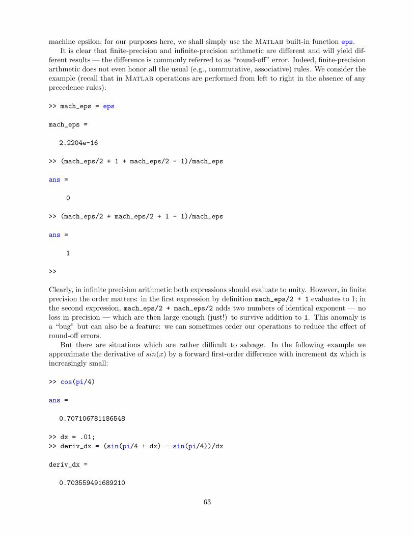
machine epsilon; for our purposes here, we shall simply use the Matlab built-in function eps.It is clear that finite-precision and infinite-precision arithmetic are different and will yield dif-

ferent results — the difference is commonly referred to as “round-off” error. Indeed, finite-precisionarthmetic does not even honor all the usual (e.g., commutative, associative) rules. We consider theexample (recall that in Matlab operations are performed from left to right in the absence of anyprecedence rules):

>> mach_eps = eps

mach_eps =

2.2204e-16

>> (mach_eps/2 + 1 + mach_eps/2 - 1)/mach_eps

ans =

0

>> (mach_eps/2 + mach_eps/2 + 1 - 1)/mach_eps

ans =

1

>>

Clearly, in infinite precision arithmetic both expressions should evaluate to unity. However, in finiteprecision the order matters: in the first expression by definition mach_eps/2 + 1 evaluates to 1; inthe second expression, mach_eps/2 + mach_eps/2 adds two numbers of identical exponent — noloss in precision — which are then large enough (just!) to survive addition to 1. This anomaly isa “bug” but can also be a feature: we can sometimes order our operations to reduce the effect ofround-off errors.

But there are situations which are rather difficult to salvage. In the following example weapproximate the derivative of sin(x) by a forward first-order difference with increment dx which isincreasingly small:

>> cos(pi/4)

ans =

0.707106781186548

>> dx = .01;

>> deriv_dx = (sin(pi/4 + dx) - sin(pi/4))/dx

deriv_dx =

0.703559491689210

63

>> dx = 1e-8;

>> deriv_dx = (sin(pi/4 + dx) - sin(pi/4))/dx

deriv_dx =

0.707106784236800

>> dx = 1e-20;

>> deriv_dx = (sin(pi/4 + dx) - sin(pi/4))/dx

deriv_dx =

0

>>

We observe that what Newton intended — and the error bound we presented in Chapter 3 — isindeed honored: as dx tends to zero the finite difference (slope) approaches the derivative (cos(π/4)).But not quite: as dx falls below machine precision, the numerator can no longer see the difference,and we obtain an O(1) error — precisely in the limit in which we should see a more and moreaccurate answer. (As the reader can no doubt guess, pi, sin, and cos are all Matlab built-infunctions.)

This is in fact very typical behavior. In order to make numerical errors small we must takesmaller increments or many degrees-of-freedom, however if we go “too far” then finite-precisioneffects unfortunately “kick in.” This trade-off could in fact be debilitating if machine precisionwere not sufficiently small, and indeed in the early days of computing with only a relatively fewbits to represent FPNs it was a struggle to balance numerical accuracy with finite precision round-off effects. These days, with the luxury of 64-bit precision, round-off errors are somewhat less of aconcern. However, there are situations in which round-off effects can become important.

In particular, we note that the problem is our derivative example is not just the numerator butalso the dx in the denominator. As a general rule, we wish to avoid — where possible — divisionby small numbers, which tends to amplify the effects of finite-precision truncation. (This relatesto stability , which is an important theme which we will encounter in many, often related, guisesin subsequent chapters.) We will see that even in much more sophisticated examples — solutionof large linear systems — “avoid division by small numbers” remains an important guideline andoften a feature (by construction) of good algorithms. The problem of course is aggravated whenwe must perform many operations as opposed to just a few operations.

We have focused our attention on addition since, as indicated, this operation is often the prox-imal cause of the round-off difficulties. Other operations are performed in the “obvious” way. Forexample, to multiply two numbers, we multiply the mantissas and add the exponents and thenre-adjust to conform to the necessary representation. Division and exponentiation follow similarrecipes. Obviously underflow and overflow can be undesired byproducts but these are typicallyeasier to avoid and not “fundamental.”

64

4.7 Relational and Logical Operations

4.7.1 Relational Operations

A relational operator performs some kind of comparison between two variables (typically floatingpoint double) and then returns a logical variable to indicate the outcome of the comparison. Therelational operators are equal, ==; not equal, ~=; less than, <; greater than, >; less than or equal, <=;greater than or equal, >=. Note that the equal operator, ==, is now interpreted in the mathematicalsense of = (vs. the Matlab assignment operator = which of course serves a different function).

As an example, we consider

>> x = 4.6; y = 4.7;

>> isless = x < y

isless =

1

>>

Here Matlab first evaluates the expression x < y — which, since x is less than y, is a truestatement, and hence returns a logical 1 — and then assigns this value of 1 to the (logical) variableisless. (As we know, floating point numbers are truncated in finite precision arithmetic; since the< operates on the truncated form, of course the comparison is only good to machine precision.)

We can of course consider composition. Typically, composition of relational operations is bylogical operations, as we now discuss. (In fact, we can apply usual arithmetic to logical variables,which are converted to floating point for the purpose. This is often convenient, but must be usedwith some care.)

4.7.2 Logical Operations

It would be possible to hi-jack operations such as + to perform Boolean operations on logicalvariables, however Matlab prefers to reserve the usual arithmetic functions for these operatorsapplied to logical variables. Hence we introduce new operators.

The three key logical operators are AND, indicated as &, OR, indicated as |, and NOT, indicatedas ~. (There are also other options, such as the exclusive or, or XOR.) The AND and OR operatorstake as (the two) operands logical variables and the result is of course also a logical variable. TheNOT takes a single logical operand and the result is also a logical variable. As already indicated,these logical operators are often composed with relational operators.

The AND, OR, and NOT behave in the expected fashion. The statement L3 = L1 & L2 yieldsL3 = 1 (true) only if both L1 and L2 are both == 1 (true), otherwise L3 = 0. The statementL3 = L1 | L2 yields L3 = 1 if either L1 == 1 or L2 == 1, otherwise L3 = 0 (note that if bothL1 == 1 and L2 == 1, then L3 = 1); conversely, L3 = 0 only if both L1 == 0 and L2 == 0. Fi-nally, the NOT: L3 = ~L1 yields L3 = 1 if L1 == 0 and L3 = 0 if L1 == 1.

As an example, we consider the AND and NOT:

>> x = 4.6; y = 4.7;

>> u = 3.1; v = 3.2;

>> z = (x < y) & ~(u < v)

65

z =

0

>>

which of course yields the correct result. Note the Matlab precedence convention is to evaluaterelational operators before logical operators and hence our parentheses in the above are redundant— but better too many parentheses than too few. And another example,

>> x = 4.6; y = 4.7;

>> u = 3.1; v = 3.2;

>> z = (x < y) | ~(u < v)

z =

1

>>

now with the OR and NOT.Finally, we mention that Matlab provides “short-circuit” versions of AND and OR, the oper-

ators for which are given by && and ||, respectively. These short-circuit operators will not evaluatethe second operand (i.e., to the right) if the first operand (i.e., to the left) suffices to make the de-cision. For example, in our OR example above, since x < y, z = (x < y) || ~(u < v) will onlyevaluate (x < y). This can lead to efficiencies — if the second operand is much more expensiveand or ensure that a (second) operand is only evaluated when it exists and is well-defined.

Logical (and relational) operations play a key role in flow control — in controlling the flow (or“direction”) of the program based on the results generated by the program itself. In some sense itis these logical and relations operations and the enabled flow control which distinguishes a programexecuted by a computer from arithmetic performed on a calculator.

4.8 Flow Control

4.8.1 The if Statement

The if statement is very simple. The general syntax is given by

if logical expression 1BLOCK 1

elseif logical expression 2BLOCK 2

else

BLOCK 3end

which is interpreted by Matlab as follows:

66

if logical expression 1 evaluates to true, execute BLOCK 1 and go to end (and continue onwith the next line in the program);

if logical expression 1 evaluates to false, but logical expression 2 evaluates to true, executeBLOCK 2 and go to end (and continue);

if logical expression 1 is false and logical expression 2 is false, execute BLOCK 3 and goto end (and continue).

Note several variants are possible: we may include multiple elseif statements between theBLOCK 1 and else; and we may omit the else and BLOCK 3 statements.

In the event that in fact there are many cases there is another Matlab statement which is nodoubt preferable to the if statement: the switch statement. We do not discuss the switch state-ment here, but rather use this opportunity to recall the very helpful help function: >> help switch

will provide you with a quick (but sufficient) description of the syntax and functionality of theswitch statement.

4.8.2 The while Statement

The syntax of the while statement is

initialize var 1, var 2,. . .while relational or logical expression while (var 1, var 2,. . . )

BLOCK % new values assigned to var 1, var 2, ...

end

This statement is a loop which is controlled by the value of the logical variable which is the result ofevaluation of relational_or_logical_expression_while. What makes the statement powerfulis that relational_or_logical_expression_while may depend on var 1, var 2, . . . , the valuesof which are changed at each pass through the loop. In particular, the while is executed as follows:if relational or logical expression while (var 1, var 2, . . . ) is true, execute (the instruction linesin) BLOCK , otherwise go to end and continue with next line of program of which the while ispart; repeat. Note that var 1, var 2, . . . must be initialized prior to entering the while loop.

As an example, we consider

>> i = 0;

>> sum_of_integers = 0;

>> while i <= 3

sum_of_integers = sum_of_integers + i;

i = i + 1;

end

>> sum

sum_of_integers =

6

>>

67

Here, relational or logical expression while (var 1) is the simple expression i <= 3, where i playsthe role of var 1. In fact, this particular sum is more easily performed with a for statement, as wedescribe shortly. The true value of the while is when the relational or logical expression is a morecomplicated function of the variables which are changed by the BLOCK and in particular when wedo not know a priori how many iterations through the loop will be required.

For example, we create the script machine eps.m

% script to calculate machine epsilon

mach_eps = 1;

while (1 + mach_eps ~= 1)

mach_eps = mach_eps/2.;

end

mach_eps

in the editor. Note that as we start to construct slightly longer programs we will start to use scriptmode rather than command-line mode. The input is easier, as are debugging and modification, andof course re-use. In addition, the editor within Matlab recognizes various keywords and automat-ically formats statements for improved readability. Note also the comment line: any material on aline which follows a % will be ignored by the interpreter and serves only to educate the author anduser’s as to the intent of the program or particular lines of the program.

We then enter in the command window

>> machine_eps

mach_eps =

1.1102e-16

>>

which runs our script. Of course this code is just calculating for us machine precision, which agreeswith the Matlab eps to within the factor of two related to our stopping tolerance.

Finally, we note that you may include a break in a BLOCK statement

if (relational or logical expression break) break

which will directly go to the end statement of the while loop quite independent of whetherrelational_or_logical_expression_while (for the current values of var 1, var 2, . . . ) is true

or false. Purists often try to avoid break statements, but pragmatists tolerate the occasionalbreak statement. Too many break statements may be a symptom of poor program design or moregenerally passive-aggressive tendencies.

4.8.3 The for Statement

The syntax for the for statement is

for VARCOUNTER = LIM 1 : INCREMENT : LIM 2BLOCK % no reassignment of VARCOUNTER

end

68

Typically LIM 1, INCREMENT, LIM 2 would be integers (even if of data type double), howeverthere are also many instances in which these variables could be (mathematically) non-integer. Notealso that INCREMENT can be positive or negative, and that if INCREMENT is not specified thenMatlab chooses the default value INCREMENT = 1.

The execution of the for loop is simple: we execute BLOCK for VARCOUNTER = LIM 1 ; weupdate VARCOUNTER = VARCOUNTER + INCREMENT ; then, if VARCOUNTER <= LIM 2 ,repeat. As for a while statement, we can interrupt the usual flow of the for loop with a break

statement. Note that if LIM 1 + INCREMENT is less than LIM 2 then BLOCK will never beexecuted.

We repeat our earlier example:

>> sum_of_integers = 0;

>> for i = 1:3

sum_of_integers = sum_of_integers + 1;

end

>> sum_of_integers

sum_of_integers =

3

>>

There are many situations in numerical methods in which the for loop is the ideal construct. How-ever, it is also true that in Matlab there are a number of functions related to array manipulationthat, although implicitly built upon a for construction, are typically more efficient than an explicitfor loop. We introduce some of these functions in the next section.

Finally, we note that our for syntax here is not as general as provided for by Matlab .However, the more general syntax requires the notions of single-index or multi-index arrays, whichwe have not yet introduced. Following the treatment of arrays the reader should do >> help for

to understand the generalization: in effect, we can require VARCOUNTER to cycle through anyparticular set of scalars (defined in a single-index array) or VARCOUNTER itself may even be asingle-index array which cycles through a particular set of single-index arrays (defined in a double-index array).

69

70

Chapter 5

Matlab Arrays

5.1 Single-Index Floating Point Arrays

5.1.1 The Concept

It is often the case that we have an ordered set of, say n, “elements” of data which are somehowrelated. The index could represent directions in three space dimensions (k = 1, 2, 3 for x, y, z,respectively) — at which we store, in each array location, the corresponding coordinate of a point(an array of length 3); or the index could represent 15 different times — at which we store, ineach location, the time of the measurement, or perhaps the measurement itself (an array of length15). Note the index plays the role of independent variable and the array value plays the role ofdependent variable. In all these cases we will often wish to operate on all n “related elements” ina similar fashion. We would thus like a way to reference all the elements with a common name,and an easy way to reference different elements through this common name, in order to developsuccinct, readable, and efficient code for implementing common operations on all the elements. Inparticular, we would not want to write n lines of code each time we wished, say, to square each ofthe n elements.

A single-index array — in this section, a floating point single-index array — is the simplest“class” which achieves these objectives. We first introduce a variable name, array name, whichshall be associated to all n elements of the array. We then index this array name in order to accessany particular element of the array: in particular, array name(i) is the pointer to element i of thearray. We emphasize that, as in the scalar case, array name(i) is not the value of element i ofthe array but rather the location in memory at which we shall store the value of element i. Forexample, array name(2) = 3.14159 would assign the value 3.14159 to the second element of thearray. (We discuss more efficient assignment methods below.)

Conceptually, you may think of the array as stored at n contiguous locations in memory. Ele-ment 1 of the array is stored in array name(1), element 2 of the array is stored in array name(2),. . . , and element n of the array is stored in array name(n). In this (virtual) sense, it suffices to(say) pass to a function simply the variable array name — which you may view as the addressof the first element — as the addresses of all the other elements of the array can then be readilydeduced from array name. (In actual practice, there is also some header information associatedwith the array — for example, in our single-index case, the length n.) Since many common arrayoperations can be performed in Matlab with simple function calls — or user-defined function

71

DRAFT V2.1 © The Authors. License: Creative Commons BY-NC-SA 3.0.

calls — at a high-level we can often deal exclusively with array name without explicit reference toparticular indices. (Of course, under the hood. . . )

5.1.2 Assignment and Access

The most explicit way to create a single-index array is by hand: X = [1,3,4] creates a single-index array of length 3, with entries X(1) = 1, X(2) = 3, and X(3) = 4. To determine thelength of an array Matlab provides a function length. In our example

>> X = [1,3,4]

X =

1 3 4

>> X(1)

ans = 1

>> length(X)

ans =

3

>>

Note that this single-index array is a row single-index array. (We can also consider column single-index arrays, in which the commas above are replaced by semi-colons: X = [1;3;4]. We reservetreatment of rows and columns to our discussion of double-index arrays.)

The input process is facilitated by the colon operator. In particular, Z = [J:D:K] createsthe single-index array J, J+ D,...,J + m*D] for m = fix((K-J)/D), where fix is a Matlabfunction which rounds to the nearest integer towards zero. (Note that J:D:K is empty if D == 0,if D > 0 & J > K, or if D < 0 & J < K.) The default value of D is 1 and hence J:K is equivalentto J:1:K, as in the example

>> firstfive = [1:5]

firstfive =

1 2 3 4 5

>>

You will in fact recognize this colon construction from the for statement; and indeed the for

statement may take the form for VARCOUNTER = S where S is any single-index array; we willrevisit this construction of the for statement shortly.

We may assign an entire array,

72

>> Y = X

Y =

1 3 4

>>

or we may assign or re-assign a particular element as, say,

>> X(3) = 10;

>> X

X =

1 3 10

>>

which we see modifies X accordingly.Of course the point of an array is that we have a systematic numerical approach to indexing,

and we may thus easily assign values with a for statement. We present two approaches. In thefirst, we zero out to initialize:

>> Z = zeros(1,10);

>> for i = 1:length(Z)

Z(i) = i^2;

end

>> Z

Z =

1 4 9 16 25 36 49 64 81 100

>>

Note that zeros(1,n) is a Matlab function which provides a (row) single-index array of all zerosof length n. (Note the first argument of zeros indicates that we wish to form a row single-indexarray; zeros(n, 1) would create a column single-index array of all zeros. We will understandzeros better once we discuss multi-index arrays.) This approach, of initialization, is preferredwhenever possible: it permits Matlab to be more efficient in memory allocation and management.

In the second approach, we concatenate:

>> Z = [];

>> for i = 1:10

Z = [Z,i^2];

end

>> Z

73

Z =

1 4 9 16 25 36 49 64 81 100

>>

Here Z = [] defines an array but the array is initially empty: we do this because we can not“add to” (append to, or concatenate to) an array which does not exist. Note that the expression[Z, i^2] evaluates to an array in which the first length(Z) elements are the elements of Z and thelast element is i^2. Thus at each iteration the length of Z grows. The above is less efficient thanthe initialization approach, but very convenient in particular (for example, in a while statement)when we do not a priori know the number of elements in our (ultimate) array.

As our last point on assignment and access, we note that Matlab supports a very convenientform of indirect addressing. In particular, if we create a single-index array of integers indvec thenwe can extract from (say) Z just those elements with indices in indvec:

>> indvec = [1,3,5,9];

>> U = Z(indvec)

U =

1 9 25 81

>>

Note you may also apply indirect addressing on the left-hand side of the assignment statement, butsome care must be exercised as regards the “shape” (row vs. column) of the resulting single-indexarray.

Note that in all these shortcuts there is always an equivalent underlying program (which is moreor less how these shortcuts are implemented). For example, in the above, an array index argumenttells Matlab to execute, effectively:

>> U_too = zeros(1,length(indvec))

>> for inew = 1:length(indvec)

U_too(inew) = Z(indvec(inew));

end

>> U_too

U_too =

1 9 25 81

>>

But of course much better to encapsulate and re-use this feature within the Matlab syntax thanto re-write this little loop on each occasion.

74

5.1.3 (Dotted) Arithmetic Operations

It is one of the major advantages of programming languages that as we develop more convenient datastructures (or types, or classes), in particular with many elements, we may also suitably define ouroperations to deal directly with these new entities — as a whole, rather than explicitly manipulatingeach element. In this section we define for the case of single-index arrays the corresponding arrayarithmetic operators.

We first discuss element-by-element operations. In these operations, we consider two arrays ofthe same length and we apply the same arithmetic operation on each pair of elements which sharethe same index. We begin with addition/subtraction (and multiplication by a scalar):

>> P = [1, 4, 7]; Q = [2, -1, 1];

>> R = P + 3.0*Q

R =

7 1 10

>>

which is simply shorthand for the loop

>> for i = 1:length(P)

R_too(i) = P(i) + 3.0*Q(i);

end

>> R_too

R_too =

7 1 10

>>

The loop makes clear the interpretation of “element by element,” but obviously the one-line state-ment is much preferred.

Note 3.0 is not an array, it is scalar , which scales all elements of the array Q in our aboveexample. This simple scaling feature can be very convenient in defining arrays of grid points or datapoints (for example, in interpolation, differentiation, and integration). To wit, if we have an intervalof length L and wish to createN segments of length L/N , we need only do >> xpts = (L/N)*[0:N].Note that xpts is of length (in the sense of number of elements in the array) N+1 since include bothendpoints: xpts(1) = 0 and xpts(N+1) = L/N.

Finally, we note one additional shortcut: if q is a scalar, then element-by-element addition toour vector P will add q to each element of P. To wit,

>> q = 3;

>> P + q

ans =

75

4 7 10

>>

We might write the above more properly as

>> P + q*ones(1,length(P))

ans =

4 7 10

>>

but there is no need given Matlab ’s automatic expansion of q when encountered in array addition.Note ones(1,n) is a Matlab function which creates a (row) single-index array of length n withall elements set to unity.

To implement element-by-element multiplication, division, and exponentiation we do

>> PdotmultQ = P.*Q

PdotmultQ =

2 -4 7

>> PdotdivideQ = P./Q

PdotdivideQ =

0.5000 -4.0000 7.0000

>> PdotexpQ = P.^Q

PdotexpQ =

1.0000 0.2500 7.0000

>>

which is equivalent to

>> for i = 1:length(P)

PdotmultQ_too(i) = P(i)*Q(i);

PdotdivideQ_too(i) = P(i)/Q(i);

PdotexpQ_too(i) = P(i)^Q(i);

end

>> PdotmultQ_too

PdotmultQ_too =

76

2 -4 7

>> PdotdivideQ_too

PdotdivideQ_too =

0.5000 -4.0000 7.0000

>> PdotexpQ_too

PdotexpQ_too =

1.0000 0.2500 7.0000

>>

As for addition, if we replace one of our vectors by a scalar, Matlab will expand out with a “ones”vector.

Why do we need the “dot” before the *, /, and ^ operators — so-called “dotted” (or element-by-element) operators: dotted multiplication, dotted division, and dotted exponentiation? It turns outthat there are two types of entities which look very similar, respectively arrays and vectors (latermulti-index arrays and matrices): both are ordered sets of n floating point numbers. However, thearithmetic operations are defined very differently for these two entities, respectively element-by-element operations for arrays and linear algebraic operations (e.g., inner products) for vectors. Wecould easily define say * to perform element-by-element multiplication for objects which are definedas arrays, and to perform an inner product for objects defined as vectors. Unfortunately, althoughconceptually quite clean, this would be very cumbersome since often in one line we wish to treat aset of numbers as an array and in the next line we wish to treat the same set of numbers as a vector:there would be much conversion and bookkeeping. Hence Matlab prefers a kind of “superclass”of array-and-vector (and matrix) entities, and hence perforce some new syntax to indicate whetherwe wish to treat the array-and-vector as an array (with dotted element-by-element operators) or avector (with undotted linear algebra operators). Note that we do not require dotted + (or dotted-) since element-by-element addition and vector addition in fact are equivalent. So there.

We note that there are many arithmetic operations on arrays in addition to element-by-elementoperations, many of which are available as Matlab functions. For example, we can easily performthe sum of the first three integers (as we did earlier with a for loop) as

>> ints = [1:3];

>> sum(ints)

ans =

6

>> mean(ints)

ans =

77

2

>>

where sum performs the sum of all the elements in an array (here ints) and mean calculates thearithmetic mean of all the element in an array.

Finally, we note here that the many Matlab built-in mathematical functions — we have alreadyencountered sin and cos, but there are many many more — look for “math function” and “specialfunctions” in the doc — which also accept single-index (and in fact, double–index) arguments. Forexample,

>> xpts = (pi/4)*0.5*[0:2];

>> sin_values = sin(xpts)

sin_values =

0 0.3827 0.7071

>>

with a single call provides the values of sin for all elements of xpts.

5.1.4 Relational and Logical (Array) Operations

For relational and logical operations we do not have the complication of array/vector conflation andhence we need no dots. In effect, when we apply any of our scalar relational/ logical operations topairs of vectors of the same length, Matlab returns a vector (of the same length as the operands)which is the result of the scalar relational/logical operation element-by-element.

As an example,

>> x = [1.2, 3.3, 2.2]; y = [-0.1, 15.6, 2.0];

>> z_1 = (x < y)

z_1 =

0 1 0

>> z_2 = (x > y)

z_2 =

1 0 1

>> z_3 = z_1 | ~z_2

z_3 =

0 1 0

78

>>

Similar example can be constructed for all of our relational operators and logical operators. Notethat z_1, z_2 and z_3 are logical arrays: each element is an instance of the logical data type.

For completeness, we indicate the implementation of the above as a for loop:

>> for i = 1:length(x)

z_1_too(i) = (x(i) < y(i));

z_2_too(i) = (x(i) > y(i));

z_3_too(i) = z_1_too(i) | ~ z_2_too(i) ;

end

>> z_1_too

z_1_too =

0 1 0

>> z_2_too

z_2_too =

1 0 1

>> z_3_too

z_3_too =

0 1 0

>>

which is indeed equivalent, but tedious.

5.1.5 “Data” Operations

There are also a number of operations which albeit numerical are focused as much on the indicesas the data — and hence we include these under the heading “data” operations.

A number of Matlab functions are available to reorder the elements or to identify distinguishedelements: sort, min, and max are perhaps the most useful in this regard. We illustrate just one ofthese functions, min:

>> T = [4.5, -2.2, 6.3, 4.4];

>> [minimum, minimizer] = min(T)

minimum =

-2.2000

79

minimizer =

2

>> minimum_too = min(T)

minimum_too =

-2.2000

>>

which yields the obvious result. This is our first example of a function with two outputs: minimumis the minimum of the array, and minimizer is the index of the minimizing element. Note also thatif we just wish to obtain the first output we can abbreviate the call.

Perhaps one of the most useful array data functions is the find function. Given a logical vectorL, find(L) will return a vector which contains (in increasing order) the indices of all the elementsof L which are nonzero (and are hence unity, since L is a logical array). (In fact, find can also beapplied to a double array, but one must be careful about round-off effects.) As an example:

>> L = logical([0,1,1,0,0,1]);

>> islogical(L)

ans =

1

>> ind_of_nonzero = find(L)

ind_of_nonzero =

2 3 6

>>

where we have also illustrated the construction of a logical vector. Note that the find functioneffectively implements the for loop

>> ind_of_nonzero_too = [];

>> for i = 1:length(L)

if( L(i) ~= 0 )

ind_of_nonzero_too = [ind_of_nonzero_too,i];

end

end

>> ind_of_nonzero_too

ind_of_nonzero_too =

2 3 6

80

>>

which demonstrates also an application of concatenation.The function find is very useful in the context of comparisons. For example, we may wish to

extract just those values of vector greater than some threshold:

>> H = [0.2, 1.4, 6.7, -3.4, 4.2];

>> log_H_thresh = (H > 1.2)

log_H_thresh =

0 1 1 0 1

>> inds_H_thresh = find(log_H_thresh)

inds_H_thresh =

2 3 5

>> H(inds_H_thresh)

ans =

1.4000 6.7000 4.2000

>>

We can of course replace H > 1.2 in the above with any more complicated composition of relationaland logical operators.

We could of course combine this as

>> H ( find ( H > 1.2 ) )

ans =

1.4000 6.7000 4.2000

>>

In fact, Matlab accepts a further abbreviation as

>> H ( H > 1.2 )

ans =

1.4000 6.7000 4.2000

>>

81

in which a find is automatically applied to a logical index vector. Apparently this somewhatsyntactically sloppy approach is in fact the most efficient.

We take this opportunity to revisit the for statement. We initially introduced the for statementof the form for VARCOUNTER = LIM_1:INC:LIM_2 and later noted that the for statement may takea more general form for VARCOUNTER = S where S is any single-index array. We now present anexample of this general form of the for statement. Our objective is to find a number of entries in a(row) single-index array that are positive. As before, we can write the for loop based on an indexas

>> scalars = [1,-3,1,2,-5];

>> num_pos = 0;

>> for i = 1:length(scalars)

if (scalars(i) > 0)

num_pos = num_pos + 1;

end

end

>> num_pos

num_pos =

3

>>

which gives the expected result. Alternatively, we may use our set of scalars directly as the argumentto the for loop. That is

>> scalars = [1,-3,1,2,-5];

>> num_pos = 0;

>> for sca = scalars

if (sca > 0)

num_pos = num_pos + 1;

end

end

>> num_pos

num_pos =

3

>>

which also gives the correct result. In this second form, within the for loop, the loop argumentsca is first set to the first element of scalars, 1, sca is then set to the second element of scalars,-3, and so on.

We may interpret the (restrictive) form of the for statement for VARCOUNTER = LIM_1:INC

:LIM_2 within this general form: LIM_1:INC:LIM_2 first yields an single-index array [LIM_1,

LIM_1+INC, ..., LIM_2] (assuming LIM_2 = LIM_1 + m*INC for some integer m); then the for

loop successively assigns an element of the array to VARCOUNTER. (We note that the argument of

82

the for loop must be a row single-index array, not a column single-index array. We revisit thispoint in our discussion of the for statement using double-index arrays.)

5.2 Characters and Character Single-Index Arrays (Strings)

Our focus is on numerical methods and hence we will not have too much demand for characterand string processing. However, it is good to know the basics, and there are instances — typicallyrelated to more sophisticated applications of software system management, “codes that write codes”(or less dramatically, codes some lines of which can be modified from case to case), and alsosymbolic manipulation — in which character concepts can play an important role. Note thatcharacter manipulation and symbolic manipulation are very different: the former does not attributeany mathematical significance to characters; the latter is built upon the former but now addsmathematical rules of engagement. We consider here only character manipulation.

A character variable (an instance of the character data type), say c, must represent a letterof numeral. As always, c ultimately must be stored (ultimately) by 0’s and 1’s. We thus need —as part of the data type definition — an encoding of different characters in terms of 0’s and 1’s.The most common such encoding, the original ASCII code, is a mapping from 8-bit words (binarynumbers) to the set of letters in the alphabet, numerals, punctuation marks, as well as some specialor control characters. (There are now many “extended” ASCII codes which include symbols fromlanguages other than English.)

We can create and assign a character variable as

>> c = '3'

c =

3

>> c_ascii = int8(c)

c_ascii =

51

>> c_too = char(c_ascii)

c_too =

3

>>

In the first statment, we enter the single-character data with quotes — which tells Matlab that3 is to be interpreted as a character and not a number. We can then obtain the ASCII codefor the number 3 — which happens to be 51. We can then recreate the character variable c bydirectly appealing to the ASCII code with the char command. Obviously, quotes are easier thanmemorizing the ASCII code.

A “string” is simply a single-index array of character elements. We can input a string most

83

easily with the quote feature:

>> pi_approx_str = '3.1416'

pi_approx_str =

3.1416

>> pi_approx_str(2)

ans =

.

>> pi_approx_str + 1

ans =

52 47 50 53 50 55

>>

We emphasize that pi_approx_str is not of type double and if we attempt to (say) add 1 topi_approx_str we get (effectively) nonsense: Matlab adds 1 to each element of the ASCII-translation of the our string according to the rules of single–index array addition.

We can readily concatenate strings, for example:

>> leader = 'The value is '

leader =

The value is

>> printstatement = [leader,pi_approx_str,' .']

printstatement =

The value is 3.1416 .

>>

However, this is of limited use since typically we would know an approximation to π not as a stringbut as double.

Fortunately, there are some simple conversion functions available in Matlab (and other pro-gramming languages as well). The Matlab function num2str will take a floating point numberand convert it to the corresponding string of characters; conversely, str2num will take a string (pre-sumably of ASCII codes for numerals) and convert it to the corresponding floating point (double)data type. So for example,

84

>> pi_approx_double = str2num(pi_approx_str)

pi_approx_double =

3.1416

>> pi_approx_str_too = num2str(pi_approx_double)

pi_approx_str_too =

3.1416

>>

This can then be used to create a print statement based on a floating point value (e.g., obtainedas part of our numerical calculations):

>> printstatement_too = [leader,num2str(pi_approx_double),' .']

printstatement_too =

The value is 3.1416 .

>>

In actual practice there are higher level printing functions (such as fprintf and sprintf) inMatlab built on the concepts described here. However, the above rather low-level constructs canalso serve, for example in developing a title for a figure which must change as (say) the time towhich the plot corresponds changes.

5.3 Double-Index Arrays

5.3.1 Concept

Double-index arrays (and more generally, multi-index arrays), are extremely important in theimplementation of numerical methods. However, conceptually, they are quite similar to single-index arrays, and inasmuch this section can be rather short: we just consider the “differentialinnovation.” In fact, as we will see shortly, a double-index array really is a single-index array asfar as internal representation in memory or “address space”: the two indices are just a convenientway to access a single-index array.

Reference by two indices (or three indices,. . . ) can be convenient for a variety of reasons: ina 10× 10 structured rectilinear mesh, the two indices might represent the location of a point in a“Cartesian” grid — at which we store, in each array location, say the value of the temperature field(a 10× 10 array); in an unstructured three-dimensional mesh (or a Monte Carlo random sample),the first index might represent the label/order of a point within a sample of say length 1000, and thesecond index might represent the spatial coordinate direction (e.g., 1, 2, 3 for the x, y, z directions)— at which we store, in the array locations, the coordinate of the point (a 1000 × 3 array); andmost notably, the two indices might represent the rows and columns of an m×n matrix — at whichwe store the matrix values (an m × n array). (We discuss matrices in depth later.) Recall that

85

the indices play the role of the independent variable and the array values the role of the dependentvariable.

For a double-index array, just as for a single-index array, we first introduce a variable name,array name, but now this double-index array is associated to m × n elements: we may think ofa double-index arrays as m rows by n columns, as we shall visualize shortly. We then index thisarray name to access any particular element of the array: in particular, array name(i,j) is thepointer to element i, j of the array. As always, the pointer is the location in memory at which westore the value of the array.

In fact, even this double-index array is stored at contiguous locations in memory. (It is inthis sense that a double-index array is internally equivalent to a single-index array; we shall takeadvantage of this equivalence later.) Matlab stores a double-index array as “first address fastest”:array name(1,1),...,array name(m,1),array name(1,2),...,array name(m,2),...,array name(m,n). As for the single-index case, it suffices to to pass to a function simply thevariable array name — the address of the first element — as the addresses of all other elements canthen be readily deduced (in practice, thanks to appropriate header information). And of course,as for a single-index array, we will endeavor to similarly define operations on the entire array, asrepresented by array name, rather than treat each index separately.

A note on nomenclature: we can also think of single-index and double-index arrays as “one-dimensional” and “two-dimensional” arrays. However, we will reserve “dimension” for the linearalgebra sense: a vector with n entries is a member of n-dimensional space. Hence the linear algebra“dimension” is analogous to the Matlab length. (And just to make sure this paragraph, inattempting to avoid confusion, is sufficiently confusing: to avoid confusion of Matlab length

with the linear algebra “length” of a vector we shall refer to the latter as the “norm” of the vector.We return to this point in Unit 3.)

5.3.2 Assignment and Access

We start with a simple example and then explain the syntax.

>> A = [1,2,3;4,5,6]

A =

1 2 3

4 5 6

>> size_of_A = size(A)

size_of_A =

2 3

>> A(2,2)

ans =

5

>>

86

We see that a comma separates elements within a row, and a semicolon separates different rows.The size function returns a single-index array of length 2: the first element is the number of rows— the limit for the first index — and the second element is the number of columns — the limit forthe second index. Finally, we see that we can access individual elements of A as (say) A(2,2). Ofcourse our interpretation as rows and columns is just an artifice — but a very useful artifice whichwe invoke on many many occasions — for visualization and interpretation.

Our row single-index array is special case of double-index array:

>> X = [1,3,4]

X =

1 3 4

>> size(X)

ans =

1 3

>> X(1,3)

ans =

4

>>

And we can now systematically introduce a column single-index array as

>> X_col = [1;3;4]

X_col =

1

3

4

>> size(X_col)

ans =

3 1

>> X_col(3,1)

ans =

4

87

>>

Note in this case each row is of length 1 so we require no comma delimiters. Note operations inMatlab require arrays of similar size, so always make sure that pairs of single-index array operandsare both row arrays or both column arrays. This is best ensured by initialization of the array withzeros and consistent assignment.

The transpose operation is very convenient: it “flips” the two indices. Hence

>> A_transp = A'

A_transp =

1 4

2 5

3 6

>> X'

ans =

1

3

4

>> size(X')

ans =

3 1

>>

Rows become columns and columns become rows. (In fact, the transpose operator is a special caseof a more general Matlab function reshape which allows us to “resize” an array.)

As always, the reader should mentally note the more expanded code which effects any particularoperation to make sure the operation is well understood: in this case

>> for i = 1:size(A,1)

for j = 1:size(A,2)

A_transp_too(j,i) = A(i,j);

end

end

>> A_transp_too

A_transp_too =

1 4

2 5

88

3 6

>>

Note that size(A,1) and size(A,2) conveniently return the first element and second element ofsize(A).

As for single-index arrays, we can directly assign an entire double-index array: B = A creates anew array B identical to A in terms of size as well as values; we may also assign or re-assign anyparticular element of the array as selected by the index — for example, B(1,1) = 0. Oftentimeswe can create the desired array as an assignment plus modification of an existing array.

We may also create an array with a “double” for loop:

>> m = 2;n = 3;

>> A = zeros(m,n);

>> for i = 1:size(A,1)

for j = 1:size(A,2)

A_too(i,j) = j + (i-1)*size(A,2);

end

end

>> A_too

A_too =

1 2 3

4 5 6

>>

Note initialization of multi-index arrays is particularly important since these arrays tend to belarger and memory management even more of an issue.

However, concatenation also works for multi-index arrays and can be very effective.

>> R1 = [1,2,3]; R2 = [4,5,6];

>> C1 = [1;4]; C2 = [2;5]; C3 = [3;6];

>> A_too_too = [R1; R2]

A_too_too =

1 2 3

4 5 6

>> A_too_too_too = [C1,C2,C3]

A_too_too_too =

1 2 3

4 5 6

>> A_four_times = [A_too, A_too; A_too, A_too]

89

A_four_times =

1 2 3 1 2 3

4 5 6 4 5 6

1 2 3 1 2 3

4 5 6 4 5 6

>> A_four_times_also = [[A_too;A_too],[A_too;A_too]]

A_four_times_also =

1 2 3 1 2 3

4 5 6 4 5 6

1 2 3 1 2 3

4 5 6 4 5 6

>> A_four_times_expand_by_one = [A_four_times,[C1;C2]; [R1,R2],0]

A_four_times_expand_by_one =

1 2 3 1 2 3 1

4 5 6 4 5 6 4

1 2 3 1 2 3 2

4 5 6 4 5 6 5

1 2 3 4 5 6 0

>>

The general procedures for concatenation are somewhat difficult to succinctly describe — we mustalways combine entities that “match” in the direction in which we concatenate — but the casesabove include most instances relevant in numerical methods.

We can also do indirect addressing for double-index arrays, as we illustrate on our arrayA_four_times. In particular, let ind1vec and ind2vec be single-index arrays given by (say)

>> ind1vec = [2,3]

ind1vec =

2 3

>> ind2vec = [2:4]

ind2vec =

2 3 4

>>

90

Then

>> extracted = A_four_times(ind1vec,ind2vec)

extracted =

5 6 4

2 3 1

>>

which in fact is implemented as

>> for i = 1:length(ind1vec)

for j = 1:length(ind2vec)

extracted_too(i,j) = A_four_times(ind1vec(i),ind2vec(j));

end

end

>> extracted_too

extracted_too =

5 6 4

2 3 1

>>

This can be very useful for extracting rows and columns, as we now describe.In particular, to extract say row 1 or column 2 of A, we need only do

>> R1_too = A(1,1:size(A,2))

R1_too =

1 2 3

>> C2_too = A(1:size(A,1),2)

C2_too =

2

5

>>

In fact, Matlab conveniently provides a function end which, when it appears in the place of kth

index (k = 1 or k = 2), evaluates to (say for our array A) size(A,k). We then can write moresuccinctly

91

>> R1_too_too = A(1,1:end)

R1_too_too =

1 2 3

>> R1_too_too_too = A(1,:)

R1_too_too_too =

1 2 3

>>

where in the last line we see that Matlab admits even further abbreviation: a colon in the placeof an index is interpreted as 1:end for that index.

Finally, there is simple way to create a single-index array from a multi-index array:

>> A_single_index = A(:)

A_single_index =

1

4

2

5

3

6

>>

Note that it is probably not a good idea to take advantage of the single-index form above as theshape of this single-index array is rather sensitive to how we specify the index argument. (Thecolon translation is not unique for a single-index array and in fact is interpreted as a particularchoice of reshape.) We introduce the above just to illustrate the concept of “all arrays are reallysingle-index arrays” and “first index fastest (or column major)” ordering, and also because thesingle-index reshape is convenient sometimes for certain global operations (see below).

5.3.3 Operations

As regards arithmetic operations, multi-index arrays “behave” in exactly the same fashion as single-index arrays: -, +, .*, ./, .^ all perform the necessary element-by-element operations. Indeed,in these operations, the double-index array is essentially treated as a single-index array. (Note thatfor example 3.2*A multiplies each element of A by 3.2.)The same is true for relational and logicaloperations (as well as find): the operations are performed element by element and the output is amulti-index array of the same size as the two operands.

For data operations, there are more options. Whenever possible, the easiest is to effect theoperation in terms of single-index arrays. The colon operator permits us to find the minimum over(say) the first row as

92

>> min(A(1,:))

ans =

1

>>

or in a similar fashion the minimum over any given column.If we wish to find the minimum over all elements of the entire array, we can interpret the

multi-index array in its “underlying” single-index form: for example,

>> A = [1,2,3;4,5,6]

A =

1 2 3

4 5 6

>> min(A(:))

ans =

1

>>

In most cases, the above simple constructs suffice.However, it is also easy to apply (say) the min function over the first index to yield a row array

which contains the minimum over each column, or to perform the min function over the secondindex to yield a column array which contains the minimum over each row:

>> min(A,[],1)

ans =

1 2 3

>> min(A,[],2)

ans =

1

4

>>

Note the second null argument in min above will be explained shortly, when we discuss functionsin greater detail. Essentially, min takes three arguments, but the second argument is optional and

93

hence if it is not set then Matlab will not complain. Nulls are useful for optional inputs or forinputs which can be set to default values.

In general the default with Matlab — when “single-index” functions are applied to multi-indexarrays — is to perform the operation over columns to yield a row:

>> min(A)

ans =

1 2 3

>>

Note that min(A) is not the same as min(A(:)) in that A is of size [2,3] whereas A(:) is auto-matically “reshaped” to be a single-index array.

We take this opportunity to revisit the for loop. Let’s say that we wish to find the number oftwo-vectors in an 2×m array which reside in the first quadrant. We can write the for loop basedon an index as

twovecs = [[1;-1],[1;1],[-3;1],[.2;.5]];

num_in_quad_1 = 0;

for j = 1:size(twovecs,2)

if( twovecs(1,j) >=0 && twovecs(2,j) >=0 )

num_in_quad_1 = num_in_quad_1 + 1;

end

end

num_in_quad_1

which will work just fine. However, we can also use for our “counter” not an index but rather thedata itself, as in

twovecs = [[1;-1],[1;1],[-3;1],[.2;.5]];

num_in_quad_1 = 0;

for vec = twovecs;

if( vec(1) >= 0 && vec(2) >= 0)

num_in_quad_1 = num_in_quad_1 + 1;

end

end

num_in_quad_1

which also works just fine. In this second form, within the for loop, the loop argument vec isfirst set to the first column of twovecs, [1;-1], vec is then set to the second columns of twovecs,[1;1], and so on. It is important to note that, for any double-index array, the loop argumentis set to each column of the array and the loop is executed the number of column times. (Inparticular, the behavior is independent of the column-grouped assignment of twovecs used in thisexample.) This also implies that, if a column single-index array is used for the loop construction asin for i = [1:10]', then i would be set to the vector [1:10]' and the loop is executed just onetime. Note that the behavior is completely different from the case of providing a row single-indexarray, as in for i = 1:10.

94

Finally, this seems a good place to note that there are many thousands of Matlab functionsand for each oftentimes quite a few options and optional arguments. If you find that you are doinga particular relatively simple operation many times — or a rather complicated operation perhapsonly a few times — it is perhaps worthwhile to search for a syntactically succinct and efficientMatlab built-in function which might do the trick. However, in many other cases it will be moreeffective to write your own code. Matlab built-in functions are a means and not an end.

5.4 Line Plotting

We include line plotting in this chapter as we now have the necessary pieces: single-index arrays,and characters. We do not present all the various options since these can readily be found by>> help plot or the documentation. However, we do provide a template which you can use andadapt accordingly.

%A sample plotting script - by Justin Miller

%----------- linear-linear plotting, sine and cosines ---------------

L = 2*pi; %Define the ending angle

N = 100; %Define number of angle segments

xpts = (L/N)*[0:N]; %Define a set of angles for plotting (in radians)

%This could also be done using

%xpts = linspace(0,L,N+1);

sin_values = sin(xpts); %Sine vector of each angle

cos_values = cos(xpts); %Cosine vector of each angle

figure %Create a figure window to draw the plots

plot(xpts,sin_values,'b-') %Plot the sine values in a blue line

hold on %Hold the current figure when plotting

%the next figure

plot(xpts,cos_values,'r--') %Plot the cosine values in a red dashed line

h_sincos_plot = gcf; %Get the handle of the current figure

ha_sincos_axis = gca; %Get the handle of the current axis

axis([0,xpts(end),-1.1,1.1]) %Set the x and y axes [xmin,xmax,ymin,ymax]

set(ha_sincos_axis,'XTick',0:pi/2:2*pi) %Set the location of the x tick marks

set(ha_sincos_axis,'YTick',-1:0.2:1) %Set the location of the y tick marks

set(ha_sincos_axis,'XTickLabel',{'0','pi/2','pi','3*pi/2','2*pi'})%Set the names of each x tick mark

95

xlabel('Angle (radians)') %Give a label name to the x axis

ylabel('Trigonomic output') %Give a label name to the y axis

title(['Plot of sin and cos from x = ',num2str(xpts(1)), ...

' to x = ',num2str(xpts(end))])%Give the figure a title

legend('sin','cos','location','best') %Provide a legend and tell matlab to place

%it in the best location

saveas(h_sincos_plot,'sin_cos.fig') %Take the figure specified by handle

%"h_sincos_plot" and save it

%as "sin_cos.fig" in the working directory

%----------- log-linear plotting, exponential ---------------

clear all

L = 5;

N = 100;

x = (L/N)*[0:N];

y = 2*exp(x);

figure

semilogy(x,y,'b-') %Create a plot where only the y axis is in log scale

%semilogx would plot only the x axis in log scale

xlabel('x')ylabel('y')

title(['Log-Linear plot of y = 2*exp(x) from x = ',num2str(x(1)), ...

' to x = ',num2str(x(end))])

saveas(gcf,'exp.fig')

%----------- log-log plotting, polynomials ---------------

clear all

L = 10^2;

N = 100;

x= (L/N)*[0:N];

y = 2*(x.^3);

figure

96

loglog(x,y,'b-') %Create a plot where both axes are in log scale

xlabel('x')ylabel('y')

title(['Log-Log plot of y = 2x^3 from x = ',num2str(x(1)), ...

' to x = ',num2str(x(end))])

saveas(gcf,'poly.fig')

Matlab also has extensive “3-D” plotting capabilities.

97

98

Chapter 6

Functions in Matlab

6.1 The Advantage: Encapsulation and Re-Use

As you know, a mathematical function is a “rule” which given some inputs (or arguments), returnsan output or outputs. A Matlab function (or a function in any programming language), is verysimilar: the function, given some inputs/arguments, returns an output or outputs. There are twomain reasons that functions are so important and useful as a programming construct: re-use andencapsulation. First, re-use: if we perform a particular set of operations — for example, calculationof sin(x) for given x — we prefer not to re-write this same code over and over again. Rather, wewrite it once and then use it over and over again, with enormous savings. Second, encapsulation: auser can take advantage of the function, and the “function” it performs — from inputs to outputs —without knowing how this function has been implemented or what is “inside” the code; from anotherperspective, what happens inside the function does not affect the user’s higher level objectives —the output is the entire “effect” (we discuss this further below).

We have already taken extensive advantage of both re-use and encapsulation: we have usedmany Matlab built-in functions in all of our examples above; and we have used these functionsnot only without knowing “what is inside” but in fact without even knowing how a function isdefined syntactically. In actual practice, it would not be good to proceed in quite such a trustingfashion.

6.2 Always Test a Function

Functions have serious implications as regards the correctness of results and the control of errors.From the positive side, the fact that the program is re-used many times, and developed onceintentionally for re-use, means that typically most bugs will have been identified and fixed. Fromthe negative side, encapsulation means that the user typically will not know what is inside, andhence can not personally vouch for correctness. The latter is, fortunately, quite easy to address ina reasonable if not rigorous fashion: confronted with any new function, it is alway worthwhile toconsider several test cases — for which you know the answer — to confirm correct behavior; themore authoritative the source, the more the function has been used, the simpler the task, perhapsthe less tests required. But remember that you are not just testing the code, you are also testingyour understanding of the inputs and outputs.

99

DRAFT V2.1 © The Authors. License: Creative Commons BY-NC-SA 3.0.

Note that is often difficult to find a test case in which we know the answer. In particular inthe numerical context there is an artifice by which to side-step this issue. In particular, it is oftenpossible to posit the answer and then easily determine the question (which yields this answer).For example, if we wish to test a code which finds the roots of a fourth-order polynomial, for anyparticular fourth-order polynomial it is not easy to deduce the correct answer (or we would notneed the code in the first place). However, it is easy to posit the four roots — the answer — andmultiply out to obtain the polynomial with these roots — the question. We then test the code bygoing backwards (in fact forwards), and verifying that the question leads to the answer. Note sucha test does not confirm that the code works in all cases; in fact, we have only confirmed one case.The numerical approach (or even the logic of the code) could thus be flawed in certain or even manyinstances. However, we have confirmed that we are using the code correctly, that we understandwhat in principle should happen, and that in at least one (or several) nontrivial cases that whatshould happen does indeed happen. You should always test a new function in this fashion.

We emphasize that our discussion here applies both to the many Matlab “built-in” functions— functions bundled with the Matlab core — and any third-party of user-defined function. Alsoin the remainder of this chapter many of the details are relevant both to built-in and user functions— for example, how to call a multi-output, multi-input function; however some details, such ashow to create a function, are obviously only important for user-defined functions.

6.3 What Happens in a Function Stays in a Function

When we launch a script (or a function) from the command window we may view this programas the “main” program (to use a somewhat archaic term). The (command-window) workspace ofthis main program is the set of variables of which the main program is aware (and which havebeen assigned at some point during the execution). When this main program calls a function, sayfunction name, we can view the process as the creation of a second virtual processor, as shownin Figure 6.1 2. In particular, it is critical to note that the two workspaces — the variablesassigned by the main program and by function name — are distinct: the main program is unawareof the variables in workspace function name and function name is unaware of the variables inworkspace command-window. The only connection between these two virtual processes are theinputs and outputs: function name receives the inputs from the main program, and the mainprogram receives the outputs from function name; note the direction of the arrows — inputs are notaffected by function name. Furthermore, workspace function name will disappear when executionof function name is completed and there will be no permanent record of workspace function name(unless of course you have written data to a file).

We make several comments. First, there are in fact ways to share variables between theworkspaces (global variables), however it is best to avoid global variables if possible since withproliferation they become a sort of programming duct tape. Second, although our picture is for amain program and a function, the same picture applies when one function calls another function(which may call another function, . . . ). In such a case the left virtual processor is associated tothe “calling program” more generally (e.g., a calling function) and the right virtual processor isassociated to the “called function.” Again, the critical point is that the workspaces of these twofunctions are distinct. Third, our picture of Figure 6.1 2 is a good mental model, but not necessarilyrepresentative of actual implementation. It is perhaps more realistic to envision an operation inwhich the “state” of the calling program is saved, the called function “takes over” the processor,and then the calling program is moved back in when the called function has returned control. Thispicture suggests that it is rather expensive to call a function, and that is indeed the case in partic-ular in Matlab ; for this reason, it is good to construct functions which, within their designated

100

Memory

I/O

InstructionStack

Interpreter

ArithmeticUnit

flowcontrol

Memory

I/O

InstructionStack

Interpreter

ArithmeticUnit

flowcontrol

inputsoutputs

main programmain program function_namefunction_name

workspace_command-windowworkspace_command-window workspace_workspace_function_namefunction_name

Figure 6.1: Two Virtual Processors

task, compute as much data as possible with each call — for example, operate on arrays ratherthan scalars — so as to minimize the number of calls. (Note this is not a recommendation to putmany different unrelated tasks or many lines of instructions within a single function since obviouslythis compromises re-use, encapsulation, and efficiency. You do not want to do too much; you justwant to operate on as much data as possible.) We discuss this further below.

6.4 Syntax: Inputs (Parameters) and Outputs

Different languages require different syntax for the definition and use (call) of a function. Wefirst consider the former and then the latter. By way of example, we present below the functionx_to_the_2p which given x evaluates the function (in this case, literally a mathematical function)x2p.

function [ value ] = x_to_the_2p( x, p )

value = x.^(2*p);

end

The first line declares that this script is a function, that the output will be returned in a variablevalue, that the function name — and also the name of the .m file in which the function is stored— is x_to_the_2p, and that the function takes two arguments, x and p. Next follows the body ofthe function which produces the output, value. The function closes with an end statement.

We note that our little function takes a single-index (or even multi-index) array as input. Ingeneral, as described above, function calls can be expensive, and hence it is best to generate asmuch data as possible with each call so as to minimize the number of calls required. For thatreason, it is often advantageous to define functions such that the (appropriate) inputs and outputsare arrays rather than scalars. (In our example above, value will be of the same size as x. This isrealized automatically through the assignment statement.) Of course scalars will be a special caseof arrays and hence the function may still be called with scalar arguments.

101

More generally the syntax for a function with J inputs and K outputs is

function [output 1, output 2, . . . , output K] = function name(input 1, input 2, ..., input J)BODY of FUNCTIONend

Note that we may have not only multiple inputs but also multiple outputs. All outputs mustbe defined within the BODY of FUNCTION or Matlab will complain.

The operation of the function is fairly clear. First our little example (which we call here from thecommand window, but of course could also be called from a “main” program or another functionprogram):

>> clear all

>> y = x_to_the_2p( [1,2], 2)

y =

1 16

>> value

??? Undefined function or variable 'value'.>>

Note in the above our function is evaluated and the output assigned to the variable y. The variablevalue is internal to the function and the calling program — in this case the function is called fromthe command-line mode and hence the calling program variables are simply the workspace — hasno knowledge of this “dummy” variable.

More generally, we call a function with J outputs and K inputs as [output 1, output 2, . . . ,output J] = function name(input 1, input 2, . . . , input J); . (Note that if we omit the semi-colon then our outputs will all be displayed in the command window.) Upon being called bythe calling program, function name executes BODY of FUNCTION for the values of the inputarguments passed to function name and then upon reaching the end statement function namereturns the outputs — and control — to the calling program. Note is possible to force an earlyreturn of a function (to the calling program) before the end statement is encountered with a return

statement within the BODY of FUNCTION .It is possible to request only the first K ′ outputs as [output 1, output 2, . . . , output K′] =

function name(input 1, input 2, . . . , input J);. Particularly useful is the case in which you onlyrequire the first output, as in this case you can directly use the function through composition withina larger expression with the intermediary of assignment. Up to this point, with the exception of min,we have considered only single-output functions (or in any event only asked for the first output) inour examples — and for precisely this composition reason. Another example here:

>> z = x_to_the_2p( [1,2], 2) + [2,3]

z =

3 19

>>

102

Note it is important to distinguish between multiple outputs and arrays. An array corresponds toa particular output, not multiple outputs; in our example above, there is a single output, whichhappens to be a single-index array of length 2.

It is also possible to call a function without all inputs specified, either with [] (null) entries orsimply with a truncated list — the first J ′ inputs. However, in this case, it is important that withinthe function all inputs that will be encountered are defined. In this regard, the Matlab functionisempty is useful (for nulls) and the Matlab nargin is useful (for truncated argument lists)in order to detect any “unset” inputs which must be assigned to default values. (Note differentprogramming languages have different mechanisms for dealing with defaults.) There is also annargout Matlab function useful in tailoring the outputs provided.

6.5 Functions of Functions: Handles

It is often the case that we wish to pass a function to a function: in other words, we wish a calledfunction to be able to operate not just on different data but also on different “input functions.” Tomake matters more concrete (and avoid using the word function too many times with reference todifferent entities), consider the function f_o_diff:

function [ value ] = f_o_diff ( func, x, delta_x )

value = (func (x + delta_x) - func (x))./delta_x;

end

This little function calculates the first-order finite difference approximation to a function funcat the point x for a given segment-length delta_x. Obviously we could include the definition offunc within f_o_diff, but then we would need to have a different derivative function for eachfunction we wished to differentiate. In contrast, f_o_diff can be re-used for any function func— clearly much preferred. (Note we could now perform a much more systematic investigation ofround-off error; in our earlier discussion we were not yet armed with functions, or arrays.)

To call f_o_diff from a calling program is quite simple with only one wrinkle within theMatlab syntax. In particular, to pass the input function func from the calling program to thecalled function (f_o_diff) we do not wish to actually pass the function but rather a kind ofpointer — or handle — to where these instructions are stored for use by any (calling) program.(The description here is virtual — a mental model which provides the right intuition. In general,what and how a programming language passes within a function call can be a rather complicatedissue.) To create a handle for the function func — in other words, to find the pointer to (say) thebeginning of the set of instructions which define func — we put an “at sign” (@) in front of funcas in @func. So for example, to apply f_o_diff to the Matlab function sin we can either do

>> sin_handle = @sin;

>> fprime = f_o_diff( sin_handle, [pi/4, pi/2], .01)

fprime =

0.7036 -0.0050

>>

103

of more directly

>> fprime_too = f_o_diff( @sin, [pi/4, pi/2], .01)

fprime_too = 0.7036 -0.0050

>>

Note handles can also be created for other kinds of objects, for example (graphics) figures.It is often the case that a function func we wish to pass to (say) function name is somehow

more general — defined with respect to more inputs — than the functions which function nameexpects. In Matlab there is an easy way to deal with this common occurrence, which we nowdiscuss.

6.6 Anonymous (or In-Line) Functions

A Matlab “anonymous” (or in-line) function is a one-liner with a single output and multipleinputs that can be defined directly in the command window or indeed on the fly in any program(possibly another function). An anonymous function has a very important property: any variablesnot defined as inputs will be assigned the current values — at the time the anonymous functionis created — within the “variable space” (e.g., workspace) of the calling program (e.g., commandwindow).

We provide a concrete example. In particular, we define an anonymous function

p = 2;

x_to_the_2p_anon = @(x) x_to_the_2p(x,p);

which is identical to x_to_the_2p but now a function of single variable, x, rather than two variables.The value of p is frozen to 2, though of course more generally we can replace p = 2 with anyexpression by which to evaluate p in terms of other variables.

To call our anonymous function, we do (following the definition above):

>> x_to_the_2p_anon([1,2])

ans =

1 16

>>

The above appears rather pointless, but it serves an important role in passing functions to otherfunctions — in particular in the context of Matlab in which there are many built-in’s that requirefunction inputs of a particular form.

Let’s say that we wish to apply our function f_o_diff to our function x_to_the_2p. Butf_o_diff is expecting a function of a single input, x, whereas x_to_the_2p has two inputs — andtwo necessary inputs, since without p we can not evaluate x_to_the_2p. This conundrum is easilyresolved with inline functions:

104

>> p = 2;

>> x_to_the_2p_anon = @(x) x_to_the_2p(x,p);

>> z = f_o_diff( x_to_the_2p_anon, [1,2], .01 )

z =

4.0604 32.2408

>>

Note that for an in-line function the function “name” is in fact the function handle (hence we needno @ in front of the x_to_the_2p_anon in the above) — the name and handle for a single-linefunction coalesce.

6.7 String Inputs and the eval Function

We note that on occasion we do want the actual function to change — the instructions to beevaluated to change — as we change the inputs. This can be done with the eval function. Thefunction eval takes as input a string and returns the evaluation of this string given current valuesfor the various variables present in the string; in essence, eval is in the interpreter.

For example, we can create the function

function [ value ] = f_o_diff_eval ( fstring, x, delta_x )

z = x;

f_x = eval(fstring);

z = x + delta_x;

f_x_plus = eval(fstring);

value = (f_x_plus - f_x)./delta_x;

end

which is our finite difference function but now with a string input fstring to specify the functionto be differentiated. Note that eval(fstring) will simply evaluate the expression fstring giventhe current values of the workspace f o diff eval.

We now call f_o_diff_eval:

>> fstring = 'z.^4';>> f_o_diff_eval(fstring,[1,2],.01)

ans =

4.0604 32.2408

>>

which gives us the same result as previously. Note that f_x = eval(fstring) in f_o_diff_eval

105

for fstring as given is equivalent to f_x = z.^4 but since in the previous line we set z = x thenf_x is assigned x.^4 as desired. Similarly, two lines down, f_x_plus is assigned the appropriatevalue since we have changed z to be z = x + delta_x. The user can now specify any desiredfunction (expressed in terms of z) without creating a Matlab function (or anonymous function).

In actual practice there are certainly better ways to accomplish these goals. The purpose ofthis little section is only to illustrate that on occasions in which we would like to adapt the actualcode there are some simple ways to implement this feature.

106

Chapter 7

Integration

7.1 Integration of Univariate Functions

Our objective is to approximate the value of the integral

I =

∫ b

af(x) dx ,

for some arbitrary univariate function f(x). Our approach to this integration problem is to ap-proximate function f by an interpolant If and to exactly integrate the interpolant, i.e.

I =N−1∑i=1

∫Si

f(x) dx ≈N−1∑i=1

∫Si

(If)(x) dx ≡ Ih . (7.1)

Recall that in constructing an interpolant, we discretize the domain [a, b] into N−1 non-overlappingsegments, delineated by segmentation points xi, i = 1, . . . , N , as illustrated in Figure 7.11 Then,we construct a polynomial interpolant on each segment using the function values at the localinterpolation points, xm, m = 1, . . . ,M . These local interpolation points can be mapped to globalfunction evaluation points, xi, i = 1, . . . , Neval. The quality of the interpolant is dictated by its typeand the segment length h, which in turn governs the quality of the integral approximation, Ih. Thesubscript h on Ih signifies that the integration is performed on a discretization with a segment lengthh. This integration process takes advantage of the ease of integrating the polynomial interpolanton each segment.

Recalling that the error in the interpolation decreases with h, we can expect the approximationof the integral Ih to approach the true integral I as h goes to 0. Let us formally establish therelationship between the interpolation error bound, emax = maxi ei, and the integration error,

1For simplicity, we assume h is constant throughout the domain.

107

DRAFT V2.1 © The Authors. License: Creative Commons BY-NC-SA 3.0.

x1

x2

x3

x4

x5

S2

discretization

x1 x2 x3

local segment S2

x1

x2

x3

x4

x5

x6

x7

x8

x9

function evaluation points

Figure 7.1: Discretization of a 1d domain into N − 1 (here N = 5) segments of length h.

|I − Ih|.

|I − Ih| =

∣∣∣∣∣∣N−1∑i=1

∫Si

(f(x)− (If)(x)) dx

∣∣∣∣∣∣ (7.2)

≤

∣∣∣∣∣∣N−1∑i=1

∫Si

|f(x)− (If)(x)| dx

∣∣∣∣∣∣ (7.3)

≤

∣∣∣∣∣∣N−1∑i=1

∫Si

ei dx

∣∣∣∣∣∣ (local interpolation error bound on Si) (7.4)

≤N−1∑i=1

ei h (definition of h) (7.5)

≤ emax

N−1∑i=1

h (definition of emax) (7.6)

= (b− a)emax . (7.7)

We make a few observations. First, the global error in the integral is a sum of the local errorcontributions. Second, since all interpolation schemes considered in Section 2.1 are convergent(emax → 0 as h → 0), the integration error also vanishes as h goes to zero. Third, while thisbound applies to any integration scheme based on interpolation, the bound is not sharp; i.e., someintegration schemes would display better convergence with h than what is predicted by the theory.

Recall that the construction of a particular interpolant is only dependent on the location of theinterpolation points and the associated function values, (xi, f(xi)), i = 1, . . . , Neval, where Neval isthe number of the (global) function evaluation points. As a result, the integration rules based onthe interpolant is also only dependent on the function values at these Neval points. Specifically, all

108

integration rules considered in this chapter are of the form

Ih =

Neval∑i=1

wif(xi) ,

where wi are the weights associated with each point and are dependent on the interpolant fromwhich the integration rules are constructed. In the context of numerical integration, the functionevaluation points are called quadrature points and the associated weights are called quadratureweights. The quadrature points and weights together constitute a quadrature rule. Not too sur-prisingly considering the Riemann integration theory, the integral is approximated as a linearcombination of the function values at the quadrature points.

Let us provide several examples of integration rules.

Example 7.1.1 rectangle rule, leftThe first integration rule considered is a rectangle rule based on the piecewise-constant, left-endpoint interpolation rule considered in Example 2.1.1. Recall the interpolant over each segmentis obtained by approximating the value of the function by a constant function that matches thevalue of the function at the left endpoint, i.e., the interpolation point is x1 = xi on segmentSi = [xi, xi+1]. The resulting integration formula is

Ih =N−1∑i=1

∫Si

(If)(x) dx =N−1∑i=1

∫Si

f(xi) dx =N−1∑i=1

hf(xi) ,

where the piecewise-constant function results in a trivial integration. Recalling that the globalfunction evaluation points, xi, are related to the segmentation points, xi, by

xi = xi, i = 1, . . . , N − 1 ,

we can also express the integration rule as

Ih =

N−1∑i=1

hf(xi) .

Figure 7.2(a) illustrates the integration rule applied to f(x) = exp(x) over [0, 1] with N = 5. Recallthat for simplicity we assume that all intervals are of the same length, h ≡ xi+1−xi, i = 1, . . . , N−1.

Let us now analyze the error associated with this integration rule. From the figure, it is clearthat the error in the integrand is a sum of the local errors committed on each segment. The localerror on each segment is the triangular gap between the interpolant and the function, which hasthe length of h and the height proportional to f ′h. Thus, the local error scales as f ′h2. Since thereare (b− a)/h segments, we expect the global integration error to scale as

|I − Ih| ∼ f ′h2(b− a)/h ∼ hf ′ .

More formally, we can apply the general integration error bound, Eq. (7.7), to obtain

|I − Ih| ≤ (b− a)emax = (b− a)h maxx∈[a,b]

|f ′(x)| .

In fact, this bound can be tightened by a constant factor, yielding

|I − Ih| ≤ (b− a)h

2maxx∈[a,b]

|f ′(x)| .

109

0 0.2 0.4 0.6 0.8 10.5

1

1.5

2

2.5

3

integral

quadrature points

function

(a) integral

1 2 4 8 16 3210

−2

10−1

100

−1.00

1/h

|I −

Ih|

(b) error

Figure 7.2: Rectangle, left-endpoint rule.

Figure 7.2(b) captures the convergence behavior of the scheme applied to the exponential function.As predicted by the theory, this integration rule is first-order accurate and the error scales as O(h).Note also that the approximation Ih underestimates the value of I if f ′ > 0 over the domain.

Before we proceed to a proof of the sharp error bound for a general f , let us analyze theintegration error directly for a linear function f(x) = mx + c. In this case, the error can beexpressed as

|I − Ih| =N−1∑i=1

∫Si

f(x)− (If)(x) dx =N−1∑i=1

∫ xi+1

xi

(mx− c)− (mxi − c) dx

=N−1∑i=1

∫ xi+1

xi

m · (x− xi) dx =N−1∑i=1

1

2m(xi+1 − xi)2

=1

2mh

N−1∑i=1

h =1

2mh(b− a) ,

Note that the integral of m · (x− xi) over Si is precisely equal to the area of the missing triangle,with the base h and the height mh. Because m = f ′(x), ∀x ∈ [a, b], we confirm that the generalerror bound is correct, and in fact sharp, for the linear function. Let us now prove the result for ageneral f .

Proof. By the fundamental theorem of calculus, we have

f(x)− (If)(x) =

∫ x

xi

f ′(ξ) dξ, x ∈ Si = [xi, xi+1] .

110

Integrating the expression over segment Si and using the Mean Value Theorem,∫Si

f(x)− (If)(x) dx =

∫ xi+1

xi

∫ x

xi

f ′(ξ) dξ dx

=

∫ xi+1

xi

(x− xi) f ′(z) dx (Mean Value Theorem, for some z ∈ [xi, x])

≤∫ xi+1

xi

|(x− xi) f ′(z)| dx

≤(∫ xi+1

xi

|x− xi| dx)

maxz∈[xi,xi+1]

|f ′(z)|

=1

2(xi+1 − xi)2 max

z∈[xi,xi+1]|f ′(z)|

≤ 1

2h2 max

x∈[xi,xi+1]|f ′(x)| .

Summing the local contributions to the integral error,

|I − Ih| =

∣∣∣∣∣∣N−1∑i=1

∫Si

f(x)− (If)(x) dx

∣∣∣∣∣∣ ≤N−1∑i=1

1

2h2 max

x∈[xi,xi+1]|f ′(x)| ≤ (b− a)

h

2maxx∈[a,b]

|f ′(x)| .

·

Example 7.1.2 rectangle rule, rightThis integration rule is based on the piecewise-constant, right-endpoint interpolation rule consideredin Example 2.1.2, in which the interpolation point is chosen as x1 = xi+1 on segment Si = [xi, xi+1].This results in the integration formula

Ih =

N−1∑i=1

∫Si

(If)(x) dx =

N−1∑i=1

∫Si

f(xi+1) dx =

N−1∑i=1

hf(xi+1) .

Recalling that global function evaluation points are related to the segmentation points by xi = xi+1,i = 1, . . . , N − 1, we also have

Ih =

N−1∑i=1

hf(xi) .

While the form of the equation is similar to the rectangle rule, left, note that the location ofthe quadrature points xi, i = 1, . . . , N − 1 are different. The integration process is illustrated inFigure 7.1.2

111

0 0.2 0.4 0.6 0.8 10.5

1

1.5

2

2.5

3

integral

quadrature points

function

Figure 7.3: Rectangle, right-endpoint rule.

This rule is very similar to the rectangle rule, left. In particular, the integration error is boundedby

|I − Ih| ≤ (b− a)h

2maxx∈[a,b]

|f ′(x)| .

The expression shows that the scheme is first-order accurate, and the rule integrates constantfunction exactly. Even though the error bounds are identical, the left- and right-rectangle rulesin general give different approximations. In particular, the right-endpoint rule overestimates I iff ′ > 0 over the domain. The proof of the error bound identical to that of the left-rectangle rule.

While the left- and right-rectangle rule are similar for integrating a static function, they exhibitfundamentally different properties when used to integrate an ordinary differential equations. Inparticular, the left- and right-integration rules result in the Euler forward and backward schemes,respectively. These two schemes exhibit completely different stability properties, which will bediscussed in chapters on Ordinary Differential Equations.

·

Example 7.1.3 rectangle rule, midpointThe third integration rule considered is based on the piecewise-constant, midpoint interpolationrule considered in Example 2.1.3. Choosing the midpoint x1 = (xi + xi+1) as the interpolationpoint for each Si = [xi, xi+1], the integration formula is given by

Ih =N−1∑i=1

∫Si

(If)(x)dx =N−1∑i=1

∫Si

f

(xi + xi+1

2

)dx =

N−1∑i=1

hf

(xi + xi+1

2

).

Recalling that the global function evaluation point of the midpoint interpolation is related to thesegmentation points by xi = (xi + xi+1)/2, i = 1, . . . , N − 1, the quadrature rule can also beexpressed as

N−1∑i=1

hf(xi) .

The integration process is illustrated in Figure 7.4(a).

112

0 0.2 0.4 0.6 0.8 10.5

1

1.5

2

2.5

3

integral

quadrature points

function

(a) integral

1 2 4 8 16 3210

−5

10−4

10−3

10−2

10−1

100

−1.00

1/h

|I −

Ih|

rectangle, left

rectangle, right

rectangle, middle

(b) error

Figure 7.4: Rectangle, midpoint rule.

The error analysis for the midpoint rule is more involved than that of the previous methods.If we apply the general error bound, Eq. (7.7), along with the interpolation error bounds for themidpoint rule, we obtain the error bound of

|I − Ih| ≤ (b− a) emax ≤ (b− a)h

2maxx∈[a,b]

|f ′(x)| .

However, this bound is not sharp. The sharp error bound for the rectangle, midpoint integrationrule is given by

|I − Ih| ≤1

24(b− a)h2 max

x∈[a,b]|f ′′(x)| .

Thus, the rectangle, midpoint rule is second-order accurate. The higher accuracy and convergencerate of the midpoint rule are captured in the error convergence plot in Figure 7.4(b).

Before we prove the error bound for a general f , let us show that the rectangle rule in factintegrates a linear function f(x) = mx+ c exactly. The integration error for a linear function canbe expressed as

I − Ih =

N−1∑i=1

∫Si

f(x)− (If)(x)dx =N−1∑i=1

∫ xi+1

xi

f(x)− f(xi + xi+1

2

)dx

=N−1∑i=1

∫ xi+1

xi

(mx+ c)−(m

(xi + xi+1

2

)+ c

)dx

=

N−1∑i=1

∫ xi+1

xi

m

[x− xi + xi+1

2

]dx .

For convenience, let us denote the midpoint of integral by xc, i.e., xc = (xi + xi+1)/2. This allowsus to express the two endpoints as xi = xc − h/2 and xi+1 = xc + h/2. We split the segment-wise

113

integral at each midpoint, yielding∫ xi+1

xi

m

[x− xi + xi+1

2

]dx =

∫ xc+h/2

xc−h/2m(x− xc) dx

=

∫ xc

xc−h/2m(x− xc) dx+

∫ xc+h/2

xc

m(x− xc) dx = 0 .

The first integral corresponds to the (signed) area of a triangle with the base h/2 and the height−mh/2. The second integral corresponds to the area of a triangle with the base h/2 and the heightmh/2. Thus, the error contribution of these two smaller triangles on Si cancel each other, and themidpoint rule integrates the linear function exactly.

Proof. For convenience, let us denote the midpoint of segment Si by xmi . The midpoint approxi-mation of the integral over Si is

Inh =

∫ xi+1

xi

f(xmi) dx =

∫ xi+1

xi

f(xmi) +m(x− xmi) dx ,

for any m. Note that the addition of he linear function with slope m that vanishes at xmi does notalter the value of the integral. The local error in the approximation is

|In − Inh | =∣∣∣∣∣∫ xi+1

xi

f(x)− f(xmi)−m(x− xmi) dx∣∣∣∣∣ .

Recall the Taylor series expansion,

f(x) = f(xmi) + f ′(xmi)(x− xmi) +1

2f ′′(ξi)(x− xmi)2 ,

for some ξi ∈ [xmi , x] (or ξi ∈ [x, xm,n] if x < xmi). Substitution of the Taylor series representationof f and m = f ′(xmi) yields

|In − Inh | =∣∣∣∣∣∫ xi+1

xi

1

2f ′′(ξi)(x− xmi)2 dx

∣∣∣∣∣ ≤∫ xi+1

xi

1

2|f ′′(ξi)(x− xmi)2| dx

≤(∫ xi+1

xi

1

2(x− xmi)2 dx

)max

ξ∈[xi,xi+1]|f ′′(ξ)| =

(1

6(x− xmi)3

∣∣∣∣xi+1

x=xi

)max

ξ∈[xi,xi+1]|f ′′(ξ)|

=1

24h3 max

ξ∈[xi,xi+1]|f ′′(ξ)| .

Summing the local contributions to the integration error, we obtain

|I − Ih| ≤N−1∑i=1

1

24h3 max

ξi∈[xi,xi+1]|f ′′(ξi)| ≤

1

24(b− a)h2 max

x∈[a,b]|f ′′(x)| .

114

The rectangle, midpoint rule belongs to a family of Newton-Cotes integration formulas, theintegration rules with equi-spaced evaluation points. However, this is also an example of Gaussquadrature, which results from picking weights and point locations for optimal accuracy. In partic-ular, k point Gauss quadrature achieves the order 2k convergence in one dimension. The midpointrule is a one-point Gauss quadrature, achieving second-order accuracy.

·In the above example, we mentioned that the midpoint rule — which exhibit second-order

convergence using just one quadrature point — is an example of Gauss quadrature rules. TheGauss quadrature rules are obtained by choosing both the quadrature points and weights in an“optimal” manner. This is in contrast to Newton-Cotes rules (e.g. trapezoidal rule), which isbased on equally spaced points. The “optimal” rule refers to the rule that maximizes the degree ofpolynomial integrated exactly for a given number of points. In one dimension, the n-point Gaussquadrature integrates 2n − 1 degree polynomial exactly. This may not be too surprising because2n − 1 degree polynomial has 2n degrees of freedom, and n-point Gauss quadrature also gives 2ndegrees of freedom (n points and n weights).

Example 7.1.4 trapezoidal ruleThe last integration rule considered is the trapezoidal rule, which is based on the linear interpolantformed by using the interpolation points x1 = xi and x2 = xi+1 on each segment Si = [xi, xi+1].The integration formula is given by

Ih =N−1∑i=1

∫Si

(If)(x) dx =N−1∑i=1

∫Si

[f(xi) +

(f(xi+1)− f(xi)

h

)(x− xi)

]

=

N−1∑i=1

[f(xi)h+

1

2(f(xi+1)− f(xi))h

]

=N−1∑i=1

1

2h(f(xi) + f(xi+1)) .

As the global function evaluation points are related to the segmentation points by xi = xi, i =1, . . . , N , the quadrature rule can also be expressed as

Ih =

N−1∑i=1

1

2h(f(xi) + f(xi+1)) ,

Rearranging the equation, we can write the integration rule as

Ih =N−1∑i=1

1

2h(f(xi) + f(xi+1)) =

1

2hf(x1) +

N−1∑i=2

[hf(xi)

]+

1

2hf(xN ) .

Note that this quadrature rule assigns a different quadrature weight to the quadrature points on thedomain boundary from the points in the interior of the domain. The integration rule is illustratedin Figure 7.5(a).

Using the general integration formula, Eq. (7.7), we obtain the error bound

|I − Ih| ≤ (b− a)emax = (b− a)h2

8maxx∈[a,b]

|f ′′(x)| .

115

0 0.2 0.4 0.6 0.8 10.5

1

1.5

2

2.5

3

integral

quadrature points

function

(a) integral

1 2 4 8 16 3210

−5

10−4

10−3

10−2

10−1

100

−1.00

−2.00

1/h

|I −

Ih|

rectangle, left

rectangle, middle

trapezoid

(b) error

Figure 7.5: Trapezoidal rule.

This bound can be tightened by a constant factor, yielding

|I − Ih| ≤ (b− a)emax = (b− a)h2

12maxx∈[a,b]

|f ′′(x)| ,

which is sharp. The error bound shows that the scheme is second-order accurate.

Proof. To prove the sharp bound of the integration error, recall the following intermediate resultfrom the proof of the linear interpolation error, Eq. (2.3),

f(x)− (If)(x) =1

2f ′′(ξi)(x− xi)(x− xi+1) ,

for some ξi ∈ [xi, xi+1]. Integrating the expression over the segment Si, we obtain the local errorrepresentation

In − Inh =

∫ xi+1

xi

f(x)− (If)(x) dx =

∫ xi+1

xi

1

2f ′′(ξi)(x− xi)(x− xi+1) dx

≤∫ xi+1

xi

1

2|f ′′(ξi)(x− xi)(x− xi+1)| dx ≤

(∫ xi+1

xi

1

2|(x− xi)(x− xi+1)| dx

)max

ξ∈[xi,xi+1]|f ′′(ξ)|

=1

12(xi+1 − xi)3 max

ξ∈[xi,xi+1]|f ′′(ξ)| = 1

12h3 max

ξ∈[xi,xi+1]|f ′′(ξ)| .

Summing the local errors, we obtain the global error bound

|I − Ih| =

∣∣∣∣∣∣N∑i=1

1

12h3 max

ξi∈[xi,xi+1]|f ′′(ξi)|

∣∣∣∣∣∣ ≤ 1

12(b− a)h2 max

x∈[a,b]|f ′′(x)| .

116

0 0.2 0.4 0.6 0.8 10

0.1

0.2

0.3

0.4

0.5

0.6

0.7

0.8

0.9

integralquadrature pointsfunction

(a) integral

1 2 4 8 16 32 64 128 25610

−4

10−3

10−2

10−1

100

−1.00

1/h

|I −

Ih|

rectangle, left

rectangle, middle

trapezoid

(b) error

Figure 7.6: Integration of a non-smooth function.

·Before concluding this section, let us make a few remarks regarding integration of a non-smooth

function. For interpolation, we saw that the maximum error can be no better than hr, where r is thehighest order derivative that is defined everywhere in the domain. For integration, the regularityrequirement is less stringent. To see this, let us again consider our discontinuous function

f(x) =

sin(πx), x ≤ 1

31

2sin(πx), x >

1

3

.

The result of applying the midpoint integration rule with eight intervals is shown in Fig-ure 7.6(a). Intuitively, we can see that the area covered by the approximation approaches thatof the true area even in the presence of the discontinuity as h → 0. Figure 7.6(b) confirms thatthis indeed is the case. All schemes considered converge at the rate of h1. The convergence ratefor the midpoint and trapezoidal rules are reduced to h1 from h2. Formally, we can show that theintegration schemes converge at the rate of min(k, r + 1), where k is the order of accuracy of theintegration scheme for a smooth problem, and r is the highest-order derivative of f that is definedeverywhere in the domain. In terms of accuracy, integration smooths and thus helps, whereasdifferentiation amplifies variations and hence hurts.

7.2 Integration of Bivariate Functions

Having interpolated bivariate functions, we now consider integration of bivariate functions. Wewish to approximate

I =

∫∫Df(x, y) dx dy .

Following the approach used to integrate univariate functions, we replace the function f by itsinterpolant and integrate the interpolant exactly.

117

(a) integral

10−2

10−1

10−5

10−4

10−3

10−2

2.00

h

|I −

Ih|

(b) error

Figure 7.7: Midpoint rule.

We triangulate the domain D as shown in Figure 2.15 for constructing interpolants. Then, weapproximate the integral as the sum of the contributions from the triangles, {Ri}Ni=1, i.e.

I =

N∑i=1

∫∫Ri

f(x, y) dx dy ≈N∑i=1

∫∫Ri

(If)(x, y) dx dy ≡ Ih .

We now consider two examples of integration rules.

Example 7.2.1 midpoint ruleThe first rule is the midpoint rule based on the piecewise-constant, midpoint interpolant. Recall,the interpolant over Ri is defined by the function value at its centroid,

(If)(x) = f(xi) = f(xci ), ∀ x ∈ Rn ,

where the centroid is given by averaging the vertex coordinates,

xi = xci =1

3

3∑i=1

xi .

The integral is approximated by

Ih =N∑i=1

∫∫Ri

(If)(x, y) dx dy =

N∑i=1

∫∫Ri

f(xi, yi) dx dy =

N∑i=1

Ai f(xi, yi) ,

where we have used the fact ∫∫Ri

dx dy = Ai ,

with Ai denoting the area of triangle Ri. The integration process is shown pictorially in Fig-ure 7.7(a). Note that this is a generalization of the midpoint rule to two dimensions.

The error in the integration is bounded by

e ≤ Ch2‖∇2f‖F .

118

(a) integral

10−2

10−1

10−5

10−4

10−3

10−2

2.00

h

|I −

Ih|

midpoint

trapezoid

(b) error

Figure 7.8: Trapezoidal rule.

Thus, the integration rule is second-order accurate. An example of error convergence is shownFigure 7.7(b), where the triangles are uniformly divided to produce a better approximation of theintegral. The convergence plot confirms the second-order convergence of the scheme.

Similar to the midpoint rule in one dimension, the midpoint rule on a triangle also belongsin the family of Gauss quadratures. The quadrature points and weights are chosen optimally toachieve as high-order convergence as possible.

·

Example 7.2.2 trapezoidal ruleThe trapezoidal-integration rule is based on the piecewise-linear interpolant. Because the integralof a linear function defined on a triangular patch is equal to the average of the function values atits vertices times the area of the triangle, the integral simplifies to

Ih =N∑i=1

1

3Ai

3∑m=1

f(xmi )

,where {x1

i , x2i , x

3i } are the vertices of the triangle Ri. The integration process is graphically shown

in Figure 7.8(a) .The error in the integration is bounded by

e ≤ Ch2‖∇2f‖F .

The integration rule is second-order accurate, as confirmed by the convergence plot shown in Fig-ure 7.8(b).

·The integration rules extend to higher dimensions in principle by using interpolation rules for

higher dimensions. However, the number of integration points increases as (1/h)d, where d is thephysical dimension. The number of points increases exponentially in d, and this is called the curseof dimensionality. An alternative is to use a integration process based on random numbers, whichis discussed in the next unit.

119

120

Unit II

Monte Carlo Methods.

121

Chapter 8

Introduction

8.1 Statistical Estimation and Simulation

8.1.1 Random Models and Phenomena

In science and engineering environments, we often encounter experiments whose outcome cannotbe determined with certainty in practice and is better described as random. An example of such arandom experiment is a coin flip. The outcome of flipping a (fair) coin is either heads (H) or tails(T), with each outcome having equal probability. Here, we define the probability of a given outcomeas the frequency of its occurrence if the experiment is repeated a large number of times.1 In otherwords, when we say that there is equal probability of heads and tails, we mean that there wouldbe an equal number of heads and tails if a fair coin is flipped a large (technically infinite) numberof times. In addition, we expect the outcome of a random experiment to be unpredictable in somesense; a coin that consistently produces a sequence HTHTHTHT or HHHTTTHHHTTT can behardly called random. In the case of a coin flip, we may associate this notion of unpredictability orrandomness with the inability to predict with certainty the outcome of the next flip by knowingthe outcomes of all preceding flips. In other words, the outcome of any given flip is independent ofor unrelated to the outcome of other flips.

While the event of heads or tails is random, the distribution of the outcome over a large numberof repeated experiments (i.e. the probability density) is determined by non-random parameters. Inthe case of a coin flip, the sole parameter that dictates the probability density is the probability ofheads, which is 1/2 for a fair coin; for a non-fair coin, the probability of heads is (by definition)different from 1/2 but is still some fixed number between 0 and 1.

Now let us briefly consider why the outcome of each coin flip may be considered random. Theoutcome of each flip is actually governed by a deterministic process. In fact, given a full descriptionof the experiment — the mass and moment of inertia of the coin, initial launch velocity, initialangular momentum, elasticity of the landing surface, density of the air, etc — we can, in principle,predict the outcome of our coin flip by solving a set of deterministic governing equations — Euler’sequations for rigid body dynamics, the Navier-Stokes equations for aerodynamics, etc. However,even for something as simple as flipping a coin, the number of variables that describe the state ofthe system is very large. Moreover, the equations that relate the state to the final outcome (i.e.

1We adhere to the frequentistic view of probability throughout this unit. We note that the Baysian view is analternative, popular interpretation of probability.

123

DRAFT V2.1 © The Authors. License: Creative Commons BY-NC-SA 3.0.

heads or tails) are complicated and the outcome is very sensitive to the conditions that governthe experiments. This renders detailed prediction very difficult, but also suggests that a randommodel — which considers just the outcome and not the myriad “uncontrolled” ways in which wecan observe the outcome — may suffice.

Although we will use a coin flip to illustrate various concepts of probability throughout thisunit due to its simplicity and our familiarity with the process, we note that random experimentsare ubiquitous in science and engineering. For example, in studying gas dynamics, the motion ofthe individual molecules is best described using probability distributions. Recalling that 1 mole ofgas contains approximately 6× 1023 particles, we can easily see that deterministic characterizationof their motion is impractical. Thus, scientists describe their motion in probabilistic terms; in fact,the macroscale velocity and temperature are parameters that describe the probability distributionof the particle motion, just as the fairness of a given coin may be characterized by the probabilityof a head. In another instance, an engineer studying the effect of gust on an airplane may useprobability distributions to describe the change in the velocity field affected by the gust. Again,even though the air motion is well-described by the Navier-Stokes equations, the highly sensitivenature of turbulence flows renders deterministic prediction of the gust behavior impractical. Moreimportantly, as the engineer is most likely not interested in the detailed mechanics that governsthe formation and propagation of the gust and is only interested in its effect on the airplane (e.g.,stresses), the gust velocity is best described in terms of a probability distribution.

8.1.2 Statistical Estimation of Parameters/Properties of Probability Distribu-tions

Statistical estimation is a process through which we deduce parameters that characterize the be-havior of a random experiment based on a sample — a set of typically large but in any event finitenumber of outcomes of repeated random experiments.2 In most cases, we postulate a probabilitydistribution — based on some plausible assumptions or based on some descriptive observations suchas crude histogram — with several parameters; we then wish to estimate these parameters. Alter-natively, we may wish to deduce certain properties — for example, the mean — of the distribution;these properties may not completely characterize the distribution, but may suffice for our predic-tive purposes. (In other cases, we may need to estimate the full distribution through an empiricalcumulative distribution function; We shall not consider this more advanced case in this text.) InChapter 9, we will introduce a variety of useful distributions, more precisely parametrized discreteprobability mass functions and continuous probability densities, as well as various properties andtechniques which facilitate the interpretation of these distributions.

Let us illustrate the statistical estimation process in the context of a coin flip. We can flipa coin (say) 100 times, record each observed outcome, and take the mean of the sample — thefraction which are heads — to estimate the probability of heads. We expect from our frequentistinterpretation that the sample mean will well approximate the probability of heads. Note that,we can only estimate — rather than evaluate — the probability of heads because evaluating theprobability of heads would require, by definition, an infinite number of experiments. We expectthat we can estimate the probability of heads — the sole parameter dictating the distribution ofour outcome — with more confidence as the sample size increases. For instance, if we wish to verifythe fairness of a given coin, our intuition tells us that we are more likely to deduce its fairness (i.e.the probability of heads equal to 0.5) correctly if we perform 10 flips than 3 flips. The probabilityof landing HHH using a fair coin in three flips — from which we might incorrectly conclude thecoin as unfair — is 1/8, which is not so unlikely, but that of landing HHHHHHHHHH in 10 flips isless than 1 in 1000 trials, which is very unlikely.

2We will provide a precise mathematical definition of sample in Chapter 10.

124

In Chapters 10 and 11, we will introduce a mathematical framework that not only allows us toestimate the parameters that characterize a random experiment but also quantify the confidencewe should have in such characterization; the latter, in turn, allows us to make claims — such as thefairness of a coin — with a given level of confidence. We consider two ubiquitous cases: a Bernoullidiscrete mass density (relevant to our coin flipping model, for example) in Chapter 10; and thenormal density in Chapter 11.

Of course, the ultimate goal of estimation is inference — prediction. In some cases the param-eters or quantities estimated, or corresponding “hypothesis tests,” in fact suffice for our purposes.In other cases, we can apply the rules of probability to make additional conclusions about how asystem will behave and in particular the probability of certain events. In some sense, we go froma finite sample of a population to a probability “law” and then back to inferences about particularevents relevant to finite samples from the population.

8.1.3 Monte Carlo Simulation

So far, we have argued that a probability distribution may be effectively used to characterize theoutcome of experiments whose deterministic characterization is impractical due to a large numberof variables governing its state and/or complicated functional dependencies of the outcome onthe state. Another instance in which a probabilistic description is favored over a deterministicdescription is when their use is computationally advantageous even if the problem is deterministic.

One example of such a problem is determination of the area (or volume) of a region whoseboundary is described implicitly. For example, what is the area of a unit-radius circle? Of course,we know the answer is π, but how might we compute the area if we did not know that A = πr2?One way to compute the area may be to tessellate (or discretize) the region into small pieces andemploy the deterministic integration techniques discussed in Chapter 7. However, application ofthe deterministic techniques becomes increasingly difficult as the region of interest becomes morecomplex. For instance, tessellating a volume intersected by multiple spheres is not a trivial task.More generally, deterministic techniques can be increasingly inefficient as the dimension of theintegration domain increases.

Monte Carlo methods are better suited for integrating over such a complicated region. Broadly,Monte Carlo methods are a class of computational techniques based on synthetically generatingrandom variables to deduce the implication of the probability distribution. Let us illustrate theidea more precisely for the area determination problem. We first note that if our region of interestis immersed in a unit square, then the area of the region is equal to the probability of a point drawnrandomly from the unit square residing in the region. Thus, if we assign a value of 0 (tail) and 1(head) to the event of drawing a point outside and inside of the region, respectively, approximatingthe area is equivalent to estimating the probability we land inside (a head). Effectively, we haveturned our area determination problem into an statistical estimation problem; the problem is nowno different from the coin flip experiment, except the outcome of each “flip” is determined byperforming a (simple) check that determines if the point drawn is inside or outside of the region.In other words, we synthetically generate a random variable (by performing the in/out check onuniformly drawn samples) and deduce the implication on the distribution (in this case the area,which is the mean of the distribution). We will study Monte-Carlo-based area integration techniquesin details in Chapter 12.

There are several advantages to using Monte Carlo methods compared to deterministic inte-gration approaches. First, Monte Carlo methods are simple to implement: in our case, we do notneed to know the domain, we only need to know whether we are in the domain. Second, MonteCarlo methods do not rely on smoothness for convergence — if we think of our integrand as 0and 1 (depending on outside or inside), our problem here is quite non-smooth. Third, although

125

Monte Carlo methods do not converge particularly quickly, the convergence rate does not degradein higher dimensions — for example, if we wished to estimate the volume of a region in a three-dimensional space. Fourth, Monte Carlo methods provide a result, along with a simple built-inerror estimator, “gradually” — useful, if not particularly accurate, answers are obtained early onin the process and hence inexpensively and quickly. Note for relatively smooth problems in smoothdomains Monte Carlo techniques are not a particularly good idea. Different methods work betterin different contexts.

Monte Carlo methods — and the idea of synthetically generating a distribution to deduce itsimplication — apply to a wide range of engineering problems. One such example is failure analysis.In the example of an airplane flying through a gust, we might be interested in the stress on the sparand wish to verify that the maximum stress anywhere in the spar does not exceed the yield strengthof the material — and certainly not the fracture strength so that we may prevent a catastrophicfailure. Directly drawing from the distribution of the gust-induced stress would be impractical;the process entails subjecting the wing to various gust and directly measuring the stress at variouspoints. A more practical approach is to instead model the gust as random variables (based onempirical data), propagate its effect through an aeroelastic model of the wing, and syntheticallygenerate the random distribution of the stress. To estimate the properties of the distribution —such as the mean stress or the probability of the maximum stress exceeding the yield stress — wesimply need to use a large enough set of realizations of our synthetically generated distribution.We will study the use of Monte Carlo methods for failure analysis in Chapter 14.

Let us conclude this chapter with a practical example of area determination problem in whichthe use of Monte Carlo methods may be advantageous.

8.2 Motivation: An Example

A museum has enlisted a camera-equipped mobile robot for surveillance purposes. The robot willnavigate the museum’s premises, pausing to take one or more 360 degree scans in each room.Figure 8.1 shows a typical room filled with various stationary obstructions (in black). We wish todetermine the vantage point in each room from which the robot will have the most unobstructedview for its scan by estimating the visible area (in white) for each candidate vantage point . We mayalso wish to provide the robot with an “onboard” visible area estimator for purposes of real-timeadaptivity, for example, if the room configuration is temporarily modified. This is a good candidatefor Monte Carlo: the domain is complex and non-smooth; we would like quick results based onrelatively few evaluations; and we wish to somehow certify the accuracy of our prediction. (Inactual practice, the computation would be performed over a three-dimensional museum room — afurther reason to consider Monte Carlo.)

We first define, for any vantage point xV and any surveillance point (to be watched) in theroom xW , the line segment S(xV ,xW ) that connects xV and xW . We can then express the areavisible from a vantage point xV as the integral

A(xV ) =

∫xW∈R such that S(xV ,xW )∩O=∅

dxW , (8.1)

where R is the room and O is the collection of obstructions. The visible area is thus defined asthe integral over all points in the room such that the line segment S(xV ,xW ) between xV and xWdoes not intersect an obstruction (or, equivalently, such that the intersection of sets S and O is thenull set).

There are many ways to do the visibility test S(xV ,xW )∩O ?= ∅, but perhaps the method most

amenable to mobile robotics is to use an “occupancy grid,” a discretization of the map in which

126

Figure 8.1: A surveillance robot scanning a room. Obstructions (in black) divide the space intovisible area (in white) and non-visible area (in gray).

0 5 10 15 20 25 30 35 40 45 50 550

5

10

15

20

25

30

35

40

x∗

y∗

Figure 8.2: Occupancy grid.

each cell’s value corresponds to the likelihood that the cell is empty or occupied. We begin byconverting our map of the room to an “occupancy grid,” a discretization of the map in which eachcell’s value corresponds to the likelihood that the cell is empty or occupied. In our case, because weknow ahead of time the layout of the room, a given cell contains either a zero if the cell is empty,or a one if it is occupied. Figure 8.2 shows a visualization of a fairly low-resolution occupancy gridfor our map, where occupied cells are shown in black.

We can use the occupancy grid to determine the visibility of a point xW in the room from agiven vantage point xV . To do this, we draw a line between the two points, determine throughwhich cells the line passes and then check the occupancy condition of each of the intervening cells.If all of the cells are empty, the point is visible. If any of the cells are occupied, the point is notvisible. Figure 8.3 shows examples of visible and non-visible cells. Once we have a method fordetermining if a point is visible or non-visible, we can directly apply our Monte Carlo methods forthe estimation of area.

127

25 30 35 40 45 5022

24

26

28

30

32

34

36

38

40

42

x∗

y∗

Figure 8.3: Visibility checking of two points from a single vantage point. Visible cells marked inblue, non-visible cells marked in red.

128

Chapter 9

Introduction to Random Variables

9.1 Discrete Random Variables

9.1.1 Probability Mass Functions

In this chapter, we develop mathematical tools for describing and analyzing random experiments,experiments whose outcome cannot be determined with certainty. A coin flip and a roll of a dieare classical examples of such experiments. The outcome of a random experiment is described bya random variable X that takes on a finite number of values,

x1, . . . , xJ ,

where J is the number of values that X takes. To fully characterize the behavior of the randomvariable, we assign a probability to each of these events, i.e.

X = xj , with probability pj , j = 1, . . . , J .

The same information can be expressed in terms of the probability mass function (pmf), or discretedensity function, fX , that assigns a probability to each possible outcome

fX(xj) = pj , j = 1, . . . , J .

In order for fX to be a valid probability density function, {pj} must satisfy

0 ≤ pj ≤ 1, j = 1, . . . , J ,

J∑j=1

pj = 1 .

The first condition requires that the probability of each event be non-negative and be less thanor equal to unity. The second condition states that {x1, . . . , xJ} includes the set of all possiblevalues that X can take, and that the sum of the probabilities of the outcome is unity. The secondcondition follows from the fact that events xi, i = 1, . . . , J , are mutually exclusive and collectivelyexhaustive. Mutually exclusive means that X cannot take on two different values of the xi’s in anygiven experiment. Collectively exhaustive means that X must take on one of the J possible valuesin any given experiment.

129

DRAFT V2.1 © The Authors. License: Creative Commons BY-NC-SA 3.0.

Note that for the same random phenomenon, we can choose many different outcomes; i.e. wecan characterize the phenomenon in many different ways. For example, xj = j could simply bea label for the j-th outcome; or xj could be a numerical value related to some attribute of thephenomenon. For instance, in the case of flipping a coin, we could associate a numerical valueof 1 with heads and 0 with tails. Of course, if we wish, we could instead associate a numericalvalue of 0 with heads and 1 with tails to describe the same experiment. We will see examples ofmany different random variables in this unit. The key point is that the association of a numericalvalue to an outcome allows us to introduce meaningful quantitative characterizations of the randomphenomenon — which is of course very important in the engineering context.

Let us define a few notions useful for characterizing the behavior of the random variable. Theexpectation of X, E[X], is defined as

E[X] =

J∑j=1

xjpj . (9.1)

The expectation of X is also called the mean. We denote the mean by µ or µX , with the secondnotation emphasizing that it is the mean of X. Note that the mean is a weighted average of thevalues taken by X, where each weight is specified according to the respective probability. This isanalogous to the concept of moment in mechanics, where the distances are provided by xj and theweights are provided by pj ; for this reason, the mean is also called the first moment. The meancorresponds to the centroid in mechanics.

Note that, in frequentist terms, the mean may be expressed as the sum of values taken by Xover a large number of realizations divided by the number of realizations, i.e.

(Mean) = lim(# Realizations)→∞

1

(# Realizations)

J∑j=1

xj · (# Occurrences of xj) .

Recalling that the probability of a given event is defined as

pj = lim(# Realizations)→∞

(# Occurrences of xj)

(# Realizations),

we observe that

E[X] =J∑j=1

xjpj ,

which is consistent with the definition provided in Eq. (9.1). Let us provide a simple gamblingscenario to clarity this frequentist interpretation of the mean. Here, we consider a “game of chance”that has J outcomes with corresponding probabilities pj , j = 1, . . . , J ; we denote by xj the (net)pay-off for outcome j. Then, in nplays plays of the game, our (net) income would be

J∑j=1

xj · (# Occurrences of xj) ,

which in the limit of large nplays (= # Realizations) yields nplays ·E[X]. In other words, the meanE[X] is the expected pay-off per play of the game, which agrees with our intuitive sense of themean.

130

The variance, or the second moment about the mean, measures the spread of the values aboutthe mean and is defined by

Var[X] ≡ E[(X − µ)2] =J∑j=1

(xj − µ)2pj .

We denote the variance as σ2. The variance can also be expressed as

Var[X] = E[(X − µ)2] =

J∑j=1

(xj − µ)2pj =

J∑j=1

(x2j − 2xjµ+ µ2)pj

=J∑j=1

x2jpj︸ ︷︷ ︸

E[X2]

−2µJ∑j=1

xjpj︸ ︷︷ ︸µ

+µ2J∑j=1

pj︸ ︷︷ ︸1

= E[X2]− µ2 .

Note that the variance has the unit of X squared. Another useful measure of the expected spreadof the random variable is standard deviation, σ, which is defined by

σ =√

Var[X] .

We typically expect departures from the mean of many standard deviations to be rare. This isparticularly the case for random variables with large range, i.e. J large. (For discrete randomvariables with small J , this spread interpretation is sometimes not obvious simply because therange of X is small.) In case of the aforementioned “game of chance” gambling scenario, thestandard deviation measures the likely (or expected) deviation in the pay-off from the expectation(i.e. the mean). Thus, the standard deviation can be related in various ways to risk; high standarddeviation implies a high-risk case with high probability of large payoff (or loss).

The mean and variance (or standard deviation) provide a convenient way of characterizing thebehavior of a probability mass function. In some cases the mean and variance (or even the meanalone) can serve as parameters which completely determine a particular mass function. In manyother cases, these two properties may not suffice to completely determine the distribution but canstill serve as useful measures from which to make further deductions.

Let us consider a few examples of discrete random variables.

Example 9.1.1 rolling a dieAs the first example, let us apply the aforementioned framework to rolling of a die. The randomvariable X describes the outcome of rolling a (fair) six-sided die. It takes on one of six possiblevalues, 1, 2, . . . , 6. These events are mutually exclusive, because a die cannot take on two differentvalues at the same time. Also, the events are exhaustive because the die must take on one of thesix values after each roll. Thus, the random variable X takes on one of the six possible values,

x1 = 1, x2 = 2, . . . , x6 = 6 .

A fair die has the equal probability of producing one of the six outcomes, i.e.

X = xj = j, with probability1

6, j = 1, . . . , 6 ,

or, in terms of the probability mass function,

fX(x) =1

6, x = 1, . . . , 6 .

131

0 20 40 60 80 100

1

2

3

4

5

6

realizations

x

x

µ

µ ± σ

(a) realization

0 0.05 0.1 0.15 0.2 0.25

1

2

3

4

5

6

fX(x)

x

pmf

frequency

(b) pmf

Figure 9.1: Illustration of the values taken by a fair six-sided die and the probability mass function.

An example of outcome of a hundred die rolls is shown in Figure 9.1(a). The die always takeson one of the six values, and there is no obvious inclination toward one value or the other. This isconsistent with the fact that any one of the six values is equally likely. (In practice, we would like tothink of Figure 9.1(a) as observed outcomes of actual die rolls, i.e. data, though for convenience herewe use synthetic data through random number generation (which we shall discuss subsequently).)

Figure 9.1(b) shows the probability mass function, fX , of the six equally likely events. The figurealso shows the relative frequency of each event — which is defined as the number of occurrences ofthe event normalized by the total number of samples (which is 100 for this case) — as a histogram.Even for a relatively small sample size of 100, the histogram roughly matches the probability massfunction. We can imagine that as the number of samples increases, the relative frequency of eachevent gets closer and closer to its value of probability mass function.

Conversely, if we have an experiment with an unknown probability distribution, we could inferits probability distribution through a large number of trials. Namely, we can construct a histogram,like the one shown in Figure 9.1(b), and then construct a probability mass function that fits thehistogram. This procedure is consistent with the frequentist interpretation of probability: theprobability of an event is the relative frequency of its occurrence in a large number of samples.The inference of the underlying probability distribution from a limited amount of data (i.e. a smallsample) is an important problem often encountered in engineering practice.

Let us now characterize the probability mass function in terms of the mean and variance. Themean of the distribution is

µ = E[X] =6∑j=1

xjpj =6∑j=1

j · 1

6=

7

2.

The variance of the distribution is

σ2 = Var[X] = E[X2]− µ26∑j=1

x2jpj − µ2 =

6∑j=1

j2 · 1

6−(

7

2

)2

=91

6− 49

4=

35

12≈ 2.9167 ,

132

and the standard deviation is

σ =√

Var[X] =

√35

12≈ 1.7078 .

·

Example 9.1.2 (discrete) uniform distributionThe outcome of rolling a (fair) die is a special case of a more general distribution, called the(discrete) uniform distribution. The uniform distribution is characterized by each event having theequal probability. It is described by two integer parameters, a and b, which assign the lower andupper bounds of the sample space, respectively. The distribution takes on J = b − a + 1 values.For the six-sided die, we have a = 1, b = 6, and J = b− a+ 1 = 6. In general, we have

xj = a+ j − 1, j = 1, . . . , J ,

fdisc.uniform(x) =1

J.

The mean and variance of a (discrete) uniform distribution are given by

µ =a+ b

2and σ2 =

J2 − 1

12.

We can easily verify that the expressions are consistent with the die rolling case with a = 1, b = 6,and J = 6, which result in µ = 7/2 and σ2 = 35/12.

Proof. The mean follows from

µ = E[X] = E[X − (a− 1) + (a− 1)] = E[X − (a− 1)] + a− 1

=

J∑j=1

(xj − (a− 1))pj + a− 1 =

J∑j=1

j1

J+ a− 1 =

1

J

J(J + 1)

2+ a− 1

=b− a+ 1 + 1

2+ a− 1 =

b+ a

2.

The variance follows from

σ2 = Var[X] = E[(X − E[X])2] = E[((X − (a− 1))− E[X − (a− 1)])2]

= E[(X − (a− 1))2]− E[X − (a− 1)]2

=

J∑j=1

(xj − (a− 1))2pj −

J∑j=1

(xj − (a− 1))pj

2

=J∑j=1

j2 1

J−

J∑j=1

jpj

2

=1

J

J(J + 1)(2J + 1)

6−[

1

J

J(J + 1)

2

]2

=J2 − 1

12=

(b− a+ 1)2 − 1

12.

133

·

Example 9.1.3 Bernoulli distribution (a coin flip)Consider a classical random experiment of flipping a coin. The outcome of a coin flip is either ahead or a tail, and each outcome is equally likely assuming the coin is fair (i.e. unbiased). Withoutloss of generality, we can associate the value of 1 (success) with head and the value of 0 (failure)with tail. In fact, the coin flip is an example of a Bernoulli experiment, whose outcome takes oneither 0 or 1.

Specifically, a Bernoulli random variable, X, takes on two values, 0 and 1, i.e. J = 2, and

x1 = 0 and x2 = 1.

The probability mass function is parametrized by a single parameter, θ ∈ [0, 1], and is given by

fXθ(x) = fBernoulli(x; θ) ≡{

1− θ, x = 0

θ, x = 1 .

In other words, θ is the probability that the random variable Xθ takes on the value of 1. Flippingof a fair coin is a particular case of a Bernoulli experiment with θ = 1/2. The θ = 1/2 case is also aspecial case of the discrete uniform distribution with a = 0 and b = 1, which results in J = 2. Notethat, in our notation, fXθ is the probability mass function associated with a particular randomvariable Xθ, whereas fBernoulli(·; θ) is a family of distributions that describe Bernoulli randomvariables. For notational simplicity, we will not explicitly state the parameter dependence of Xθ onθ from hereon, unless the explicit clarification is necessary, i.e. we will simply use X for the randomvariable and fX for its probability mass function. (Also note that what we call a random variableis of course our choice, and, in the subsequent sections, we often use variable B, instead of X, fora Bernoulli random variable.)

Examples of the values taken by Bernoulli random variables with θ = 1/2 and θ = 1/4 areshown in Figure 9.2. As expected, with θ = 1/2, the random variable takes on the value of 0 and 1roughly equal number of times. On the other hand, θ = 1/4 results in the random variable takingon 0 more frequently than 1.

The probability mass functions, shown in Figure 9.2, reflect the fact that θ = 1/4 results in Xtaking on 0 three times more frequently than 1. Even with just 100 samples, the relative frequencyhistograms captures the difference in the frequency of the events for θ = 1/2 and θ = 1/4. Infact, even if we did not know the underlying pmf — characterized by θ in this case — we can inferfrom the sampled data that the second case has a lower probability of success (i.e. x = 1) thanthe first case. In the subsequent chapters, we will formalize this notion of inferring the underlyingdistribution from samples and present a method for performing the task.

The mean and variance of the Bernoulli distribution are given by

E[X] = θ and Var[X] = θ(1− θ) .

Note that lower θ results in a lower mean, because the distribution is more likely to take on thevalue of 0 than 1. Note also that the variance is small for either θ → 0 or θ → 1 as in these caseswe are almost sure to get one or the other outcome. But note that (say) σ/E(X) scales as 1/

√(θ)

(recall σ is the standard deviation) and hence the relative variation in X becomes more pronouncedfor small θ: this will have important consequences in our ability to predict rare events.

134

0 20 40 60 80 100

0

1

realizations

x

x

µ

(a) realization, θ = 1/2

0 0.1 0.2 0.3 0.4 0.5 0.6 0.7

0

1

fX(x)

x

pmf

frequency

(b) pmf, θ = 1/2

0 20 40 60 80 100

0

1

realizations

x

x

µ

(c) realization, θ = 1/4

0 0.2 0.4 0.6 0.8 1

0

1

fX(x)

x

pmf

frequency

(d) pmf, θ = 1/4

Figure 9.2: Illustration of the values taken by Bernoulli random variables and the probability massfunctions.

135

Proof. Proof of the mean and variance follows directly from the definitions. The mean is given by

µ = E[X] =

J∑j=1

xjpj = 0 · (1− θ) + 1 · θ = θ .

The variance is given by

Var[X] = E[(X − µ)2] =J∑j=1

(xj − µ)2pj = (0− θ)2 · (1− θ) + (1− θ)2 · θ = θ(1− θ) .

·Before concluding this subsection, let us briefly discuss the concept of “events.” We can define

an event of A or B as the random variable X taking on one of some set of mutually exclusiveoutcomes xj in either the set A or the set B. Then, we have

P (A or B) = P (A ∪B) = P (A) + P (B)− P (A ∩B).

That is, probability of event A or B taking place is equal to double counting the outcomes xj inboth A and B and then subtracting out the outcomes in both A and B to correct for this doublecounting. Note that, if A and B are mutually exclusive, we have A ∩ B = ∅ and P (A ∩ B) = 0.Thus the probability of A or B is

P (A or B) = P (A) + P (B), (A and B mutually exclusive).

This agrees with our intuition that if A and B are mutually exclusive, we would not double countoutcomes and thus would not need to correct for it.

9.1.2 Transformation

Random variables, just like deterministic variables, can be transformed by a function. For example,if X is a random variable and g is a function, then a transformation

Y = g(X)

produces another random variable Y . Recall that we described the behavior of X that takes onone of J values by

X = xj with probability pj , j = 1, . . . , J .

The associated probability mass function was fX(xj) = pj , j = 1, . . . , J . The transformationY = g(X) yields the set of outcomes yj , j = 1, . . . , J , where each yj results from applying g to xj ,i.e.

yj = g(xj), j = 1, . . . , J .

Thus, Y can be described by

Y = yj = g(xj) with probability pj , j = 1, . . . , J .

136

We can write the probability mass function of Y as

fY (yj) = fY (g(xj)) = pj j = 1, . . . , J .

We can express the mean of the transformed variable in a few different ways:

E[Y ] =J∑j=1

yjfY (yj) =J∑j=1

yjpj =J∑j=1

g(xj)fX(xj) .

The first expression expresses the mean in terms of Y only, whereas the final expression expressesE[Y ] in terms of X and g without making a direct reference to Y .

Let us consider a specific example.

Example 9.1.4 from rolling a die to flipping a coinLet us say that we want to create a random experiment with equal probability of success and failure(e.g. deciding who goes first in a football game), but all you have is a die instead of a coin. One wayto create a Bernoulli random experiment is to roll the die, and assign “success” if an odd numberis rolled and assign “failure” if an even number is rolled.

Let us write out the process more formally. We start with a (discrete) uniform random variableX that takes on

xj = j, j = 1, . . . , 6 ,

with probability pj = 1/6, j = 1, . . . , 6. Equivalently, the probability density function for X is

fX(x) =1

6, x = 1, 2, . . . , 6 .

Consider a function

g(x) =

{0, x ∈ {1, 3, 5}1, x ∈ {2, 4, 6} .

Let us consider a random variable Y = g(X). Mapping the outcomes of X, x1, . . . , x6, to y′1, . . . , y′6,

we have

y′1 = g(x1) = g(1) = 0 ,

y′2 = g(x2) = g(2) = 1 ,

y′3 = g(x3) = g(3) = 0 ,

y′4 = g(x4) = g(4) = 1 ,

y′5 = g(x5) = g(5) = 0 ,

y′6 = g(x6) = g(6) = 1 .

We could thus describe the transformed variable Y as

Y = y′j with probability pj = 1/6, j = 1, . . . , 6 .

However, because y′1 = y′3 = y′5 and y′2 = y′4 = y′6, we can simplify the expression. Without lossof generality, let us set

y1 = y′1 = y′3 = y′5 = 0 and y2 = y′2 = y′4 = y′6 = 1 .

137

1 2 3 4 5 6

0

1

fX(1)=1/6 1/6 1/6

1/6 1/6 1/6

fY(0)=1/2

fY(1)=1/2

x

y =

g(x

)

Figure 9.3: Transformation of X associated with a die roll to a Bernoulli random variable Y .

We now combine the frequentist interpretation of probability with the fact that x1, . . . , x6 aremutually exclusive. Recall that to a frequentist, P (Y = y1 = 0) is the probability that Y takes on0 in a large number of trials. In order for Y to take on 0, we must have x = 1, 3, or 5. BecauseX taking on 1, 3, and 5 are mutually exclusive events (e.g. X cannot take on 1 and 3 at the sametime), the number of occurrences of y = 0 is equal to the sum of the number of occurrences ofx = 1, x = 3, and x = 5. Thus, the relative frequency of Y taking on 0 — or its probability — isequal to the sum of the relative frequencies of X taking on 1, 3, or 5. Mathematically,

P (Y = y1 = 0) = P (X = 1) + P (X = 3) + P (X = 5) =1

6+

1

6+

1

6=

1

2.

Similarly, because X taking on 2, 4, and 6 are mutually exclusive events,

P (Y = y2 = 1) = P (X = 2) + P (X = 4) + P (X = 6) =1

6+

1

6+

1

6=

1

2.

Thus, we have

Y =

{0, with probability 1/2

1, with probability 1/2 ,

or, in terms of the probability density function,

fY (y) =1

2, y = 0, 1 .

Note that we have transformed the uniform random variable X by the function g to create aBernoulli random variable Y . We emphasize that the mutually exclusive property of x1, . . . , x6 is thekey that enables the simple summation of probability of the events. In essence, (say), y = 0 obtainsif x = 1 OR if x = 3 OR if x = 5 (a union of events) and since the events are mutually exclusivethe “number of events” that satisfy this condition — ultimately (when normalized) frequency orprobability — is the sum of the individual “number” of each event. The transformation procedureis illustrated in Figure 9.3.

Let us now calculate the mean of Y in two different ways. Using the probability density of Y ,we can directly compute the mean as

E[Y ] =

2∑j=1

yjfY (yj) = 0 · 1

2+ 1 · 1

2=

1

2.

138

Or, we can use the distribution of X and the function g to compute the mean

E[Y ] =6∑j=1

g(xj)fX(xj) = 0 · 1

6+ 1 · 1

6+ 0 · 1

6+ 1 · 1

6+ 0 · 1

6+ 1 · 1

6=

1

2.

Clearly, both methods yield the same mean.

·

9.2 Discrete Bivariate Random Variables (Random Vectors)

9.2.1 Joint Distributions

So far, we have consider scalar random variables, each of whose outcomes is described by a singlevalue. In this section, we extend the concept to random variables whose outcome are vectors. Forsimplicity, we consider a random vector of the form

(X,Y ) ,

where X and Y take on JX and JY values, respectively. Thus, the random vector (X,Y ) takeson J = JX · JY values. The probability mass function associated with (X,Y ) is denoted by fX,Y .Similar to the scalar case, the probability mass function assigns a probability to each of the possibleoutcomes, i.e.

fX,Y (xi, yj) = pij , i = 1, . . . , JX , j = 1, . . . , JY .

Again, the function must satisfy

0 ≤ pij ≤ 1, i = 1, . . . , JX , j = 1, . . . , JY ,

JY∑j=1

JX∑i=1

pij = 1 .

Before we introduce key concepts that did not exist for a scalar random variable, let us give asimple example of joint probability distribution.

Example 9.2.1 rolling two diceAs the first example, let us consider rolling two dice. The first die takes on xi = i, i = 1, . . . , 6,and the second die takes on yj = j, j = 1, . . . , 6. The random vector associated with rolling thetwo dice is

(X,Y ) ,

where X takes on JX = 6 values and Y takes on JY = 6 values. Thus, the random vector (X,Y )takes on J = JX · JY = 36 values. Because (for a fair die) each of the 36 outcomes is equally likely,the probability mass function fX,Y is

fX,Y (xi, yj) =1

36, i = 1, . . . , 6, j = 1, . . . , 6 .

The probability mass function is shown graphically in Figure 9.4.

·

139

1 2 3 4 5 6

1

2

3

4

5

6

x

y1/36 1/36 1/36 1/36 1/36 1/36

1/36 1/36 1/36 1/36 1/36 1/36

1/36 1/36 1/36 1/36 1/36 1/36

1/36 1/36 1/36 1/36 1/36 1/36

1/36 1/36 1/36 1/36 1/36 1/36

1/36 1/36 1/36 1/36 1/36 1/36

Figure 9.4: The probability mass function for rolling two dice..

9.2.2 Characterization of Joint Distributions

Now let us introduce a few additional concepts useful for describing joint distributions. Throughoutthis section, we consider a random vector (X,Y ) with the associated probability distribution fX,Y .First is the marginal density , which is defined as

fX(xi) =

JY∑j=1

fX,Y (xi, yj), i = 1, . . . , JX .

In words, marginal density of X is the probability distribution of X disregarding Y . That is, weignore the outcome of Y , and ask ourselves the question: How frequently does X take on the valuexi? Clearly, this is equal to summing the joint probability fX,Y (xi, jj) for all values of yj . Similarly,the marginal density for Y is

fY (yj) =

JX∑i=1

fX,Y (xi, yj), j = 1, . . . , JY .

Again, in this case, we ignore the outcome of X and ask: How frequently does Y take on the valueyj? Note that the marginal densities are valid probability distributions because

fX(xi) =

JY∑j=1

fX,Y (xi, yj) ≤JX∑k=1

JY∑j=1

fX,Y (xk, yj) = 1, i = 1, . . . , JX ,

and

JX∑i=1

fX(xi) =

JX∑i=1

JY∑j=1

fX,Y (xi, yj) = 1 .

The second concept is the conditional probability , which is the probability that X takes on thevalue xi given Y has taken on the value yj . The conditional probability is denoted by

fX|Y (xi|yj), i = 1, . . . , JX , for a given yj .

140

The conditional probability can be expressed as

fX|Y (xi|yj) =fX,Y (xi, yj)

fY (yj).

In words, the probability that X takes on xi given that Y has taken on yj is equal to the probabilitythat both events take on (xi, yj) normalized by the probability that Y takes on yj disregarding xi.We can consider a different interpretation of the relationship by rearranging the equation as

fX,Y (xi, yj) = fX|Y (xi|yj)fY (yj) (9.2)

and then summing on j to yield

fX(xi) =

JY∑j=1

f(xi, yj) =

JY∑j=1

fX|Y (xi|yj)fY (yj) .

In other words, the marginal probability of X taking on xi is equal to the sum of the probabilities ofX taking on xi given Y has taken on yj multiplied by the probability of Y taking on yj disregardingxi.

From (9.2), we can derive Bayes’ law (or Bayes’ theorem), a useful rule that relates conditionalprobabilities of two events. First, we exchange the roles of x and y in (9.2), obtaining

fY,X(yj , xi) = fY |X(yj |xi)fX(xi).

But, since fY,X(yj , xi) = fX,Y (xi, yj),

fY |X(yj |xi)fX(xi) = fX|Y (xi|yj)fY (yj),

and rearranging the equation yields

fY |X(yj |xi) =fX|Y (xi|yj)fY (yj)

fX(xi). (9.3)

Equation (9.3) is called Bayes’ law. The rule has many useful applications in which we might knowone conditional density and we wish to infer the other conditional density. (We also note the the-orem is fundamental to Bayesian statistics and, for example, is exploited in estimation and inverseproblems — problems of inferring the underlying parameters of a system from measurements.)

Example 9.2.2 marginal and conditional density of rolling two diceLet us revisit the example of rolling two dice, and illustrate how the marginal density and conditionaldensity are computed. We recall that the probability mass function for the problem is

fX,Y (x, y) =1

36, x = 1, . . . , 6, y = 1, . . . , 6 .

The calculation of the marginal density of X is illustrated in Figure 9.5(a). For each xi,i = 1, . . . , 6, we have

fX(xi) =

6∑j=1

fX,Y (xi, yj) =1

36+

1

36+

1

36+

1

36+

1

36+

1

36=

1

6, i = 1, . . . , 6 .

We can also deduce this from intuition and arrive at the same conclusion. Recall that marginaldensity of X is the probability density of X ignoring the outcome of Y . For this two-dice rolling

141

1 2 3 4 5 6

1

2

3

4

5

6

x

y

1/36 1/36 1/36 1/36 1/36 1/36

1/36 1/36 1/36 1/36 1/36 1/36

1/36 1/36 1/36 1/36 1/36 1/36

1/36 1/36 1/36 1/36 1/36 1/36

1/36 1/36 1/36 1/36 1/36 1/36

1/36 1/36 1/36 1/36 1/36 1/36

1/6 1/6 1/6 1/6 1/6 1/6

(a) marginal density, fX

1 2 3 4 5 6

1

2

3

4

5

6

x

y

1/36 1/36 1/36 1/36 1/36 1/36

1/36 1/36 1/36 1/36 1/36 1/36

1/36 1/36 1/36 1/36 1/36 1/36

1/36 1/36 1/36 1/36 1/36 1/36

1/36 1/36 1/36 1/36 1/36 1/36

1/36 1/36 1/36 1/36 1/36 1/36

1/6

1/6

1/6

1/6

1/6

1/6

(b) marginal density, fY

Figure 9.5: Illustration of calculating marginal density fX(x = 2) and fY (y = 3).

example, it simply corresponds to the probability distribution of rolling a single die, which is clearlyequal to

fX(x) =1

6, x = 1, . . . , 6 .

Similar calculation of the marginal density of Y , fY , is illustrated in Figure 9.5(b). In this case,ignoring the first die (X), the second die produces yj = j, j = 1, . . . , 6, with the equal probabilityof 1/6.

Let us now illustrate the calculation of conditional probability. As the first example, let uscompute the conditional probability of X given Y . In particular, say we are given y = 3. Asshown in Figure 9.6(a), the joint probability of all outcomes except those corresponding to y = 3are irrelevant (shaded region). Within the region with y = 3, we have six possible outcomes, eachwith the equal probability. Thus, we have

fX|Y (x|y = 3) =1

6, x = 1, . . . , 6 .

Note that, we can compute this by simply considering the select set of joint probabilities fX,Y (x, y =3) and re-normalizing the probabilities by their sum. In other words,

fX|Y (x|y = 3) =fX,Y (x, y = 3)∑6i=1 fX,Y (xi, y = 3)

=fX,Y (x, y = 3)

fY (y = 3),

which is precisely equal to the formula we have introduced earlier.Similarly, Figure 9.6(b) illustrates the calculation of the conditional probability fY |X(y, x = 2).

In this case, we only consider joint probability distribution of fX,Y (x = 2, y) and re-normalize thedensity by fX(x = 2).

·A very important concept is independence. Two events are said to be independent if the

occurrence of one event does not influence the outcome of the other event. More precisely, tworandom variables X and Y are said to be independent if their probability density function satisfies

fX,Y (xi, yj) = fX(xi) · fY (yj), i = 1, . . . , JX , j = 1, . . . , JY .

142

1 2 3 4 5 6

1

2

3

4

5

6

1/6 1/6 1/6 1/6 1/6 1/6

x

y

1/36 1/36 1/36 1/36 1/36 1/36

1/36 1/36 1/36 1/36 1/36 1/36

1/36 1/36 1/36 1/36 1/36 1/36

1/36 1/36 1/36 1/36 1/36 1/36

1/36 1/36 1/36 1/36 1/36 1/36

1/36 1/36 1/36 1/36 1/36 1/36

(a) conditional density, fX|Y (x|y = 3)

1 2 3 4 5 6

1

2

3

4

5

6

1/6

1/6

1/6

1/6

1/6

1/6

x

y

1/36 1/36 1/36 1/36 1/36 1/36

1/36 1/36 1/36 1/36 1/36 1/36

1/36 1/36 1/36 1/36 1/36 1/36

1/36 1/36 1/36 1/36 1/36 1/36

1/36 1/36 1/36 1/36 1/36 1/36

1/36 1/36 1/36 1/36 1/36 1/36

(b) conditional density, fY |X(y|x = 2)

Figure 9.6: Illustration of calculating conditional density fX|Y (x|y = 3) and fY |X(y|x = 2).

The fact that the probability density is simply a product of marginal densities means that we candraw X and Y separately according to their respective marginal probability and then form therandom vector (X,Y ).

Using conditional probability, we can connect our intuitive understanding of independence withthe precise definition. Namely,

fX|Y (xi|yj) =fX,Y (xi, yj)

fY (yj)=fX(xi)fY (yj)

fY (yj)= fX(xi) .

That is, the conditional probability of X given Y is no different from the probability that X takeson x disregarding y. In other words, knowing the outcome of Y adds no additional informationabout the outcome of X. This agrees with our intuitive sense of independence.

We have discussed the notion of “or” and related it to the union of two sets. Let us now brieflydiscuss the notion of “and” in the context of joint probability. First, note that fX,Y (x, y) is theprobability that X = x and Y = y, i.e. fX,Y (x, y) = P (X = x and Y = y). More generally,consider two events A and B, and in particular A and B, which is the intersection of A and B,A ∩B. If the two events are independent, then

P (A and B) = P (A)P (B)

and hence fX,Y (x, y) = fX(x)fY (y) which we can think of as probability of P (A ∩B). Pictorially,we can associate event A with X taking on a specified value as marked in Figure 9.5(a) and eventB with Y taking on a specified value as marked in Figure 9.5(b). The intersection of A and B is theintersection of the two marked regions, and the joint probability fX,Y is the probability associatedwith this intersection.

To solidify the idea of independence, let us consider two canonical examples involving coin flips.

Example 9.2.3 independent events: two random variables associated with two inde-pendent coin flipsLet us consider flipping two fair coins. We associate the outcome of flipping the first and secondcoins with random variables X and Y , respectively. Furthermore, we associate the values of 1 and

143

0 1

0

1

x

y

1/4

1/4

1/4

1/4

fY(0)=1/2

fY(1)=1/2

fX(0)=1/2 f

X(1)=1/2

Figure 9.7: The probability mass function for flipping two independent coins.

0 to head and tail, respectively. We can associate the two flips with a random vector (X,Y ), whosepossible outcomes are

(0, 0), (0, 1), (1, 0), and (1, 1) .

Intuitively, the two variables X and Y will be independent if the outcome of the second flip,described by Y , is not influenced by the outcome of the first flip, described by X, and vice versa.

We postulate that it is equally likely to obtain any of the four outcomes, such that the jointprobability mass function is given by

fX,Y (x, y) =1

4, (x, y) ∈ {(0, 0), (0, 1), (1, 0), (1, 1)} .

We now show that this assumption implies independence, as we would intuitively expect. Inparticular, the marginal probability density of X is

fX(x) =1

2, x ∈ {0, 1} ,

since (say) P (X = 0) = P ((X,Y ) = (0, 0)) + P ((X,Y ) = (0, 1)) = 1/2. Similarly, the marginalprobability density of Y is

fY (y) =1

2, y ∈ {0, 1} .

We now note that

fX,Y (x, y) = fX(x) · fY (y) =1

4, (x, y) ∈ {(0, 0), (0, 1), (1, 0), (1, 1)} ,

which is the definition of independence.The probability mass function of (X,Y ) and the marginal density of X and Y are shown in

Figure 9.7. The figure clearly shows that the joint density of (X,Y ) is the product of the marginaldensity of X and Y . Let us show that this agrees with our intuition, in particular by consideringthe probability of (X,Y ) = (0, 0). First, the relative frequency that X takes on 0 is 1/2. Second, ofthe events in which X = 0, 1/2 of these take on Y = 0. Note that this probability is independentof the value that X takes. Thus, the relative frequency of X taking on 0 and Y taking on 0 is 1/2of 1/2, which is equal to 1/4.

144

0 1

0

1

x

y

0

1/2

1/2

0

Figure 9.8: The probability mass function for flipping two independent coins.

We can also consider conditional probability of an event that X takes on 1 given that Y takeson 0. The conditional probability is

fX|Y (x = 1|y = 0) =fX,Y (x = 1, y = 0)

fY (y = 0)=

1/4

1/2=

1

2.

This probability is equal to the marginal probability of fX(x = 1). This agrees with our intuition;given that two events are independent, we gain no additional information about the outcome of Xfrom knowing the outcome of Y .

·

Example 9.2.4 non-independent events: two random variables associated with a singlecoin flipLet us now consider flipping a single coin. We associate a Bernoulli random variables X and Ywith

X =

{1, head

0, tailand Y =

{1, tail

0, head.

Note that a head results in (X,Y ) = (1, 0), whereas a tail results in (X,Y ) = (0, 1). Intuitively,the random variables are not independent, because the outcome of X completely determines Y , i.e.X + Y = 1.

Let us show that these two variables are not independent. We are equally like to get a head,(1, 0), or a tail, (0, 1). We cannot produce (0, 0), because the coin cannot be head and tail at thesame time. Similarly, (1, 1) has probably of zero. Thus, the joint probability density function is

fX,Y (x, y) =

12 , (x, y) = (0, 1)12 , (x, y) = (1, 0)

0, (x, y) = (0, 0) or (x, y) = (1, 1) .

The probability mass function is illustrated in Figure 9.8.The marginal density of each of the event is the same as before, i.e. X is equally likely to take

on 0 or 1, and Y is equally like to take on 0 or 1. Thus, we have

fX(x) =1

2, x ∈ {0, 1}

fY (y) =1

2, y ∈ {0, 1} .

145

For (x, y) = (0, 0), we have

fX,Y (x, y) = 0 6= 1

4= fX(x) · fY (y) .

So, X and Y are not independent.We can also consider conditional probabilities. The conditional probability of x = 1 given that

y = 0 is

fX|Y (x = 1|y = 0) =fX,Y (x = 1, y = 0)

fY (y = 0)=

1/2

1/2= 1 .

In words, given that we know Y takes on 0, we know that X takes on 1. On the other hand, theconditional probability of x = 1 given that y = 1 is

fX|Y (x = 0|y = 0) =fX,Y (x = 0, y = 0)

fY (y = 0)=

0

1/2= 0 .

In words, given that Y takes on 1, there is no way that X takes on 1. Unlike the previous examplethat associated (X,Y ) with two independent coin flips, we know with certainty the outcome of Xgiven the outcome of Y , and vice versa.

·We have seen that independence is one way of describing the relationship between two events.

Independence is a binary idea; either two events are independent or not independent. Anotherconcept that describes how closely two events are related is correlation, which is a normalizedcovariance. The covariance of two random variables X and Y is denoted by Cov(X,Y ) and definedas

Cov(X,Y ) ≡ E[(X − µX)(Y − µY )] .

The correlation of X and Y is denoted by ρXY and is defined as

ρXY =Cov(X,Y )

σXσY,

where we recall that σX and σY are the standard deviation of X and Y , respectively. The correlationindicates how strongly two random events are related and takes on a value between −1 and 1. Inparticular, two perfectly correlated events take on 1 (or −1), and two independent events take on0.

Two independent events have zero correlation because

Cov(X,Y ) = E[(X − µX)(Y − µY )] =

JY∑j=1

JX∑i=1

(xi − µX)(yj − µY )fX,Y (xi, yj)

=

JY∑j=1

JX∑i=1

(xi − µX)(yj − µY )fX(xi)fY (yj)

=

JY∑j=1

(yj − µY )fY (yj)

· JX∑i=1

(xi − µX)fX(xi)

= E[Y − µY ] · E[X − µX ] = 0 · 0 = 0 .

The third inequality follows from the definition of independence, fX,Y (xi, yj) = fX(xi)fY (yj).Thus, if random variables are independent, then they are uncorrelated. However, the converse isnot true in general.

146

9.3 Binomial Distribution

In the previous section, we saw random vectors consisting of two random variables, X and Y . Letus generalize the concept and introduce a random vector consisting of n components

(X1, X2, . . . , Xn) ,

where each Xi is a random variable. In particular, we are interested in the case where each Xi isa Bernoulli random variable with the probability of success of θ. Moreover, we assume that Xi,i = 1, . . . , n, are independent. Because the random variables are independent and each variable hasthe same distribution, they are said to be independent and identically distributed or i.i.d. for short.In other words, if a set of random variables X1, . . . , Xn is i.i.d., then

fX1,X2,...,Xn(x1, x2, . . . , xn) = fX(x1) · fX(x2) · · · fX(xn) ,

where fX is the common probability density for X1, . . . , Xn. This concept plays an importantrole in statistical inference and allows us to, for example, make a probabilistic statement aboutbehaviors of random experiments based on observations.

Now let us transform the i.i.d. random vector (X1, . . . , Xn) of Bernoulli random variables to arandom variable Z by summing its components, i.e.

Zn =n∑i=1

Xi .

(More precisely we should write Zn,θ since Z depends on both n and θ.) Note Zn is a function of(X1, X2, . . . , Xn), and in fact a simple function — the sum. Because Xi, i = 1, . . . , n, are randomvariables, their sum is also a random variable. In fact, this sum of Bernoulli random variableis called a binomial random variable. It is denoted by Zn ∼ B(n, θ) (shorthand for fZn,θ(z) =

fbinomial(z;n, θ)), where n is the number of Bernoulli events and θ is the probability of success ofeach event. Let us consider a few examples of binomial distributions.

Example 9.3.1 total number of heads in flipping two fair coinsLet us first revisit the case of flipping two fair coins. The random vector considered in this case is

(X1, X2) ,

where X1 and X2 are independent Bernoulli random variables associated with the first and secondflip, respectively. As in the previous coin flip cases, we associate 1 with heads and 0 with tails.There are four possible outcome of these flips,

(0, 0), (0, 1), (1, 0), and (1, 1) .

From the two flips, we can construct the binomial distribution Z2 ∼ B(2, θ = 1/2), corresponding tothe total number of heads that results from flipping two fair coins. The binomial random variableis defined as

Z2 = X1 +X2 .

Counting the number of heads associated with all possible outcomes of the coin flip, the binomialrandom variable takes on the following value:

First flip 0 0 1 1Second flip 0 1 0 1

Z2 0 1 1 2

147

Because the coin flips are independent and each coin flip has the probability density of fXi(x) = 1/2,x = 0, 1, their joint distribution is

fX1,X2(x1, x2) = fX1(x1) · fX2(x2) =1

2· 1

2=

1

4, (x1, x2) ∈ {(0, 0), (0, 1), (1, 0), (1, 1)} .

In words, each of the four possible events are equally likely. Of these four equally likely events,Z2 ∼ B(2, 1/2) takes on the value of 0 in one event, 1 in two events, and 2 in one event. Thus, thebehavior of the binomial random variable Z2 can be concisely stated as

Z2 =

0, with probability 1/4

1, with probability 1/2 (= 2/4)

2, with probability 1/4 .

Note this example is very similar to Example 9.1.4: Z2, the sum of X1 and X2, is our g(X); weassign probabilities by invoking the mutually exclusive property, OR (union), and summation. Notethat the mode, the value that Z2 is most likely to take, is 1 for this case. The probability massfunction of Z2 is given by

fZ2(x) =

1/4, x = 0

1/2, x = 1

1/4, x = 2 .

·

Example 9.3.2 total number of heads in flipping three fair coinsLet us know extend the previous example to the case of flipping a fair coin three times. In thiscase, the random vector considered has three components,

(X1, X2, X3) ,

with each X1 being a Bernoulli random variable with the probability of success of 1/2. From thethree flips, we can construct the binomial distribution Z3 ∼ B(3, 1/2) with

Z3 = X1 +X2 +X3 .

The all possible outcomes of the random vector and the associated outcomes of the binomialdistribution are:

First flip 0 1 0 0 1 0 1 1Second flip 0 0 1 0 1 1 0 1Third flip 0 0 0 1 0 1 1 1

Z3 0 1 1 1 2 2 2 3

Because the Bernoulli random variables are independent, their joint distribution is

fX1,X2,X3(x1, x2, x3) = fX1(x1) · fX2(x2) · fX3(x3) =1

2· 1

2· 1

2=

1

8.

In other words, each of the eight events is equally likely. Of the eight equally likely events, Z3 takeson the value of 0 in one event, 1 in three events, 2 in three events, and 3 in one event. The behavior

148

of the binomial variable Z3 is summarized by

Z3 =

0, with probability 1/8

1, with probability 3/8

2, with probability 3/8

3, with probability 1/8 .

The probability mass function (for θ = 1/2) is thus given by

fZ3(x) =

1/8, x = 0

3/8, x = 1

3/8, x = 2

1/8, x = 3 .

·

Example 9.3.3 total number of heads in flipping four fair coinsWe can repeat the procedure for four flips of fair coins (n = 4 and θ = 1/2). In this case, weconsider the sum of the entries of a random vector consisting of four Bernoulli random variables,(X1, X2, X3, X4). The behavior of Z4 = B(4, 1/2) is summarized by

Z4 =

0, with probability 1/16

1, with probability 1/4

2, with probability 3/8

3, with probability 1/4

4, with probability 1/16 .

Note that Z4 is much more likely to take on the value of 2 than 0, because there are many equally-likely events that leads to Z4 = 2, whereas there is only one event that leads to Z4 = 0. In general,as the number of flips increase, the deviation of Zn ∼ B(n, θ) from nθ becomes increasingly unlikely.

·Figure 9.9 illustrates the values taken by binomial random variables for n = 2 and n = 4, both

with θ = 1/2. The histogram confirms that the distribution is more likely to take on the valuesnear the mean because there are more sequences of the coin flips that realizes these values. Wealso note that the values become more concentrated near the mean, nθ, relative to the range of thevalues it can take, [0, n], as n increases. This is reflected in the decrease in the standard deviationrelative to the width of the range of the values Zn can take.

In general, a binomial random variable Zn ∼ B(n, θ) behaves as

Zn = k, with probability

(nk

)θk(1− θ)n−k ,

where k = 1, . . . , n. Recall that

(nk

)is the binomial coefficient, read “n choose k: the number

of ways of picking k unordered outcomes from n possibilities. The value can be evaluated as(nk

)≡ n!

(n− k)!k!, (9.4)

149

0 20 40 60 80 100

0

1

2

realizations

x

x

µ

µ ± σ

(a) realization, n = 2, θ = 1/2

0 0.1 0.2 0.3 0.4 0.5 0.6 0.7

0

1

2

fX(x)

x

pmf

frequency

(b) pmf, n = 2, θ = 1/2

0 20 40 60 80 100

0

1

2

3

4

realizations

x

x

µ

µ ± σ

(c) realization, n = 4, θ = 1/2

0 0.1 0.2 0.3 0.4 0.5

0

1

2

3

4

fX(x)

x

pmf

frequency

(d) pmf, n = 4, θ = 1/2

Figure 9.9: Illustration of the values taken by binomial random variables.

150

where ! denotes the factorial.We can readily derive the formula for B(n, θ). We think of n tosses as a binary number with n

bits, and we ask how many ways k ones can appear. We can place the first one in n different places,the second one in n− 1 different places, . . . , which yields n!/(n− k)! possibilities. But since we arejust counting the number of ones, the order of appearance does not matter, and we must dividen!/(n− k)! by the number of different orders in which we can construct the same pattern of k ones— the first one can appear in k places, the second one in k − 1 places, . . . , which yields k!. Thusthere are “n choose k” ways to obtain k ones in a binary number of length n, or equivalently “nchoose k” different binary numbers with k ones. Next, by independence, each pattern of k ones (andhence n − k zeros) has probability θk(1 − θ)n−k. Finally, by the mutually exclusive property, theprobability that Zn = k is simply the number of patterns with k ones multiplied by the probabilitythat each such pattern occurs (note the probability is the same for each such pattern).

The mean and variance of a binomial distribution is given by

E[Zn] = nθ and Var[Zn] = nθ(1− θ) .

Proof. The proof for the mean follows from the linearity of expectation, i.e.

E[Zn] = E

n∑i=1

Xi

=n∑i=1

E[Xi] =n∑i=1

θ = nθ .

Note we can readily prove that the expectation of the sum is the sum of the expectations. Weconsider the n-dimensional sum over the joint mass function of the Xi weighted — per the definitionof expectation — by the sum of the Xi, i = 1, . . . , n. Then, for any given Xi, we factorize the jointmass function: n− 1 of the sums then return unity, while the last sum gives the expectation of Xi.The proof for variance relies on the pairwise independence of the random variables

Var[Zn] = E[(Zn − E[Zn])2] = E

n∑i=1

Xi

− nθ

2 = E

n∑i=1

(Xi − θ)

2

= E

n∑i=1

(Xi − θ)2 +

n∑i=1

n∑j=1j 6=i

(Xi − θ)(Xj − θ)

=

n∑i=1

E[(Xi − θ)2] +n∑i=1

n∑j=1j 6=i

((((((((

((E[(Xi − θ)(Xj − θ)]

=n∑i=1

Var[Xi] =n∑i=1

θ(1− θ) = nθ(1− θ) .

The cross terms cancel because coin flips are independent.

Note that the variance scales with n, or, equivalently, the standard deviation scales with√n. This

turns out to be the key to Monte Carlo methods — numerical methods based on random variables— which is the focus of the later chapters of this unit.

151

Let us get some insight to how the general formula works by applying it to the binomialdistribution associated with flipping coins three times.

Example 9.3.4 applying the general formula to coin flipsLet us revisit Z3 = B(3, 1/2) associated with the number of heads in flipping three coins. Theprobability that Z3 = 0 is, by substituting n = 3, k = 0, and θ = 1/2,

fZ3(0) =

(nk

)θk(1− θ)n−k =

(30

)(1

2

)0(1− 1

2

)3−0

=3!

0!(3− 0)!

(1

2

)3

=1

8,

which is consistent with the probability we obtained previously. Let us consider another case: theprobability of Z3 = 2 is

fZ3(2) =

(nk

)θk(1− θ)n−k =

(32

)(1

2

)2(1− 1

2

)3−2

=3!

2!(3− 2)!

(1

2

)3

=3

8.

Note that the θk(1− θ)n−k is the probability that the random vector of Bernoulli variables

(X1, X2, . . . , Xn) ,

realizes X1 = X2 = . . . = Xk = 1 and Xk+1 = . . . = Xn = 0, and hence Zn = k. Then, we multiplythe probability with the number of different ways that we can realize the sum Zn = k, which isequal to the number of different way of rearranging the random vector. Here, we are using thefact that the random variables are identically distributed. In the special case of (fair) coin flips,θk(1− θ)n−k = (1/2)k(1− 1/2)n−k = (1/2)n, because each random vector is equally likely.

·

9.4 Continuous Random Variables

9.4.1 Probability Density Function; Cumulative Distribution Function

Let X be a random variable that takes on any real value in (say) an interval,

X ∈ [a, b] .

The probability density function (pdf) is a function over [a, b], fX(x), such that

fX(x) ≥ 0, ∀x ∈ [a, b] ,∫ b

afX(x) dx = 1 .

Note that the condition that the probability mass function sums to unity is replaced by an integralcondition for the continuous variable. The probability that X take on a value over an infinitesimalinterval of length dx is

P (x ≤ X ≤ x+ dx) = fX(x) dx ,

or, over a finite subinterval [a′, b′] ⊂ [a, b],

P (a′ ≤ X ≤ b′) =

∫ b′

a′fX(x) dx .

152

In other words, the probability that X takes on the value between a′ and b′ is the integral of theprobability density function fX over [a′, b′].

A particular instance of this is a cumulative distribution function (cdf), FX(x), which describesthe probability that X will take on a value less than x, i.e.

FX(x) =

∫ x

afX(x) dx .

(We can also replace a with −∞ if we define fX(x) = 0 for −∞ < x < a.) Note that any cdfsatisfies the conditions

FX(a) =

∫ a

afX(x) dx = 0 and FX(b) =

∫ b

afX(x) dx = 1 .

Furthermore, it easily follows from the definition that

P (a′ ≤ X ≤ b′) = FX(b′)− FX(a′).

That is, we can compute the probability of X taking on a value in [a′, b′] by taking the differenceof the cdf evaluated at the two end points.

Let us introduce a few notions useful for characterizing a pdf, and thus the behavior of therandom variable. The mean, µ, or the expected value, E[X], of the random variable X is

µ = E[X] =

∫ b

af(x) x dx .

The variance, Var(X), is a measure of the spread of the values that X takes about its mean and isdefined by

Var(X) = E[(X − µ)2] =

∫ b

a(x− µ)2f(x) dx .

The variance can also be expressed as

Var(X) = E[(X − µ)2] =

∫ b

a(x− µ)2f(x) dx

=

∫ b

ax2f(x) dx− 2µ

∫ b

axf(x) dx︸ ︷︷ ︸µ

+µ2

∫ b

af(x) dx

= E[X2]− µ2 .

The α-th quantile of a random variable X is denoted by zα and satisfies

FX(zα) = α.

In other words, the quantile zα partitions the interval [a, b] such that the probability of X takingon a value in [a, zα] is α (and conversely P (zα ≤ X ≤ b) = 1 − α). The α = 1/2 quantile is themedian.

Let us consider a few examples of continuous random variables.

153

−1 −0.5 0 0.5 1 1.5 2 2.5 3

0

0.1

0.2

0.3

0.4

0.5

0.6

0.7

0.8

0.9

1

a=0.0, b=1.0

a=−0.5, b=2.0

(a) probability density function

−1 −0.5 0 0.5 1 1.5 2 2.5 3

0

0.1

0.2

0.3

0.4

0.5

0.6

0.7

0.8

0.9

1

a=0.0, b=1.0

a=−0.5, b=2.0

(b) cumulative density function

Figure 9.10: Uniform distributions

Example 9.4.1 Uniform distributionLet X be a uniform random variable. Then, X is characterized by a constant pdf,

fX(x) = funiform(x; a, b) ≡ 1

b− a .

Note that the pdf satisfies the constraint∫ b

afX(x) dx =

∫ b

afuniform(x; a, b) dx =

∫ b

a

1

b− a dx = 1 .

Furthermore, the probability that the random variable takes on a value in the subinterval [a′, b′] ∈[a, b] is

P (a′ ≤ X ≤ b′) =

∫ b′

a′fX(x) dx =

∫ b′

a′funiform(x; a, b) dx =

∫ b′

a′

1

b− a dx =b′ − a′b− a .

In other words, the probability that X ∈ [a′, b′] is proportional to the relative length of the intervalas the density is equally distributed. The distribution is compactly denoted as U(a, b) and wewrite X ∼ U(a, b). A straightforward integration of the pdf shows that the cumulative distributionfunction of X ∼ U(a, b) is

FX(x) = F uniform(x; a, b) ≡ x− ab− a .

The pdf and cdf for a few uniform distributions are shown in Figure 9.10.An example of the values taken by a uniform random variable U(0, 1) is shown in Figure 9.11(a).

By construction, the range of values that the variable takes is limited to between a = 0 and b = 1.As expected, there is no obvious concentration of the values within the range [a, b]. Figure 9.11(b)shows a histrogram that summarizes the frequency of the event that X resides in bins [xi, xi + δx],i = 1, . . . , nbin. The relative frequency of occurrence is normalized by δx to be consistent withthe definition of the probability density function. In particular, the integral of the region filledby the histogram is unity. While there is some spread in the frequencies of occurrences due to

154

0 20 40 60 80 100−0.2

0

0.2

0.4

0.6

0.8

1

realizations

x

x

µ

µ ± σ

(a) realization

0 0.5 1 1.5−0.2

0

0.2

0.4

0.6

0.8

1

fX(x)

x

pdf

frequency

(b) probability density

Figure 9.11: Illustration of the values taken by an uniform random variable (a = 0, b = 1).

the relatively small sample size, the histogram resembles the probability density function. This isconsistent with the frequentist interpretation of probability.

The mean of the uniform distribution is given by

E[X] =

∫ b

axfX(x) dx =

∫ b

ax

1

b− a dx =1

2(a+ b) .

This agrees with our intuition, because if X is to take on a value between a and b with equalprobability, then the mean would be the midpoint of the interval. The variance of the uniformdistribution is

Var(X) = E[X2]− (E[X])2 =

∫ b

ax2fX(x) dx−

(1

2(a+ b)

)2

=

∫ b

a

x2

b− a dx−(

1

2(a+ b)

)2

=1

12(b− a)2 .

·

Example 9.4.2 Normal distributionLet X be a normal random variable. Then the probability density function of X is of the form

fX(x) = fnormal(x;µ, σ2) ≡ 1√2πσ

exp

(−(x− µ)2

2σ2

).

The pdf is parametrized by two variables, the mean µ and the variance σ2. (More precisely wewould thus write Xµ,σ2 .) Note that the density is non-zero over the entire real axis and thus inprinciple X can take on any value. The normal distribution is concisely denoted by X ∼ N (µ, σ2).The cumulative distribution function of a normal distribution takes the form

FX(x) = F normal(x;µ, σ2) ≡ 1

2

[1 + erf

(x− µ√

2σ

)],

155

−10 −5 0 5 100

0.1

0.2

0.3

0.4

0.5

0.6

0.7

µ=0.0, σ2=1.0

µ=0.0, σ2=0.5

µ=0.0, σ2=4.0

µ=4.0, σ2=4.0

(a) probability density function

−10 −5 0 5 10

0

0.1

0.2

0.3

0.4

0.5

0.6

0.7

0.8

0.9

1

µ=0.0, σ2=1.0

µ=0.0, σ2=0.5

µ=0.0, σ2=4.0

µ=4.0, σ2=4.0

(b) cumulative density function

Figure 9.12: Normal distributions

where erf is the error function, given by

erf(x) =2

π

∫ x

0e−z

2dz .

We note that it is customary to denote the cdf for the standard normal distribution (i.e. µ = 0,σ2 = 1) by Φ, i.e.

Φ(x) = F normal(x;µ = 0, σ2 = 1).

We will see many use of this cdf in the subsequent sections. The pdf and cdf for a few normaldistributions are shown in Figure 9.12.

An example of the values taken by a normal random variable is shown in Figure 9.13. Asalready noted, X can in principle take on any real value; however, in practice, as the Gaussianfunction decays quickly away from the mean, the probability of X taking on a value many standarddeviations away from the mean is small. Figure 9.13 clearly illustrates that the values taken byX is clustered near the mean. In particular, we can deduce from the cdf that X takes on valueswithin σ, 2σ, and 3σ of the mean with probability 68.2%, 95.4%, and 99.7%, respectively. In otherwords, the probability of X taking of the value outside of µ± 3σ is given by

1−∫ µ+3σ

µ−3σfnormal(x;µ, σ2) dx ≡ 1− (F normal(µ+ 3σ;µ, σ2)− F normal(µ− 3σ;µ, σ2)) ≈ 0.003 .

We can easily compute a few quantiles based on this information. For example,

z0.841 ≈ µ+ σ, z0.977 ≈ µ+ 2σ, and z0.9987 ≈ µ+ 3σ.

It is worth mentioning that z0.975 ≈ µ + 1.96σ, as we will frequently use this constant in thesubsequent sections.

·Although we only consider either discrete or continuous random variables in this notes, random

variables can be mixed discrete and continuous in general. Mixed discrete-continuous randomvariables are characterized by the appearance of discontinuities in their cumulative distributionfunction.

156

0 20 40 60 80 100−4

−3

−2

−1

0

1

2

3

4

realizations

x

x

µ

µ ± σ

(a) realization

0 0.1 0.2 0.3 0.4 0.5−4

−3

−2

−1

0

1

2

3

4

fX(x)

x

pdf

frequency

(b) probability density

Figure 9.13: Illustration of the values taken by a normal random variable (µ = 0, σ = 1).

9.4.2 Transformations of Continuous Random Variables

Just like discrete random variables, continuous random variables can be transformed by a function.The transformation of a random variable X by a function g produces another random variable, Y ,and we denote this by

Y = g(X) .

We shall consider here only monotonic functions g.Recall that we have described the random variable X by distribution

P (x ≤ X ≤ x+ dx) = fX(x) dx .

The transformed variable follows

P (y ≤ Y ≤ y + dy) = fY (y) dy .

Substitution of y = g(x) and dy = g′(x)dx and noting g(x) + g′(x)dx = g(x+ dx) results in

fY (y) dy = P (g(x) ≤ g(X) ≤ g(x) + g′(x) dx) = P (g(x) ≤ g(X) ≤ g(x+ dx))

= P (x ≤ X ≤ x+ dx) = fX(x) dx .

In other words, fY (y)dy = fX(x) dx. This is the continuous analog to fY (yj) = pj = fX(xj) in thediscrete case.

We can manipulate the expression to obtain an explicit expression for fY in terms of fX and g.First we note (from monotonicity) that

y = g(x) ⇒ x = g−1(y) and dx =dg−1

dydy .

Substitution of the expressions in fY (y)dy = fX(x) dx yields

fY (y) dy = fX(x) dx = fX(g−1(y)) · dg−1

dydy

157

or,

fY (y) = fX(g−1(y)) · dg−1

dy.

Conversely, we can also obtain an explicit expression for fX in terms of fY and g. From y = g(x)and dy = g′(x) dx, we obtain

fX(x) dx = fY (y) dy = fY (g(x)) · g′(x) dx ⇒ fX(x) = fY (g(x)) · g′(x) .

We shall consider several applications below.Assuming X takes on a value between a and b, and Y takes on a value between c and d, the

mean of Y is

E[Y ] =

∫ d

cyfY (y) dy =

∫ b

ag(x)fX(x) dx ,

where the second equality follows from fY (y) dy = fX(x) dx and y = g(x).

Example 9.4.3 Standard uniform distribution to a general uniform distributionAs the first example, let us consider the standard uniform distribution U ∼ U(0, 1). We wish togenerate a general uniform distribution X ∼ U(a, b) defined on the interval [a, b]. Because a uniformdistribution is uniquely determined by the two end points, we simply need to map the end point 0to a and the point 1 to b. This is accomplished by the transformation

g(u) = a+ (b− a)u .

Thus, X ∼ U(a, b) is obtained by mapping U ∼ U(0, 1) as

X = a+ (b− a)U .

Proof. Proof follows directly from the transformation of the probability density function. Theprobability density function of U is

fU (u) =

{1, u ∈ [0, 1]

0, otherwise.

The inverse of the transformation x = g(u) = a+ (b− a)u is

g−1(x) =x− ab− a .

From the transformation of the probability density function, fX is

fX(x) = fU (g−1(x)) · dg−1

dx= fU

(x− ab− a

)· 1

b− a .

We note that fU evaluates to 1 if

0 ≤ x− ab− a ≤ 1 ⇒ a ≤ x ≤ b ,

and fU evaluates to 0 otherwise. Thus, fX simplifies to

fX(x) =

{1b−a , x ∈ [a, b]

0, otherwise ,

which is precisely the probability density function of U(a, b).

158

·

Example 9.4.4 Standard uniform distribution to a discrete distributionThe uniform distribution can also be mapped to a discrete random variable. Consider a discreterandom variable Y takes on three values (J = 3), with

y1 = 0, y2 = 2, and y3 = 3

with probability

fY (y) =

1/2, y1 = 0

1/4, y2 = 2

1/4, y3 = 3

.

To generate Y , we can consider a discontinuous function g. To get the desired discrete probabilitydistribution, we subdivide the interval [0, 1] into three subintervals of appropriate lengths. Inparticular, to generate Y , we consider

g(x) =

0, x ∈ [0, 1/2)

2, x ∈ [1/2, 3/4)

3, x ∈ [3/4, 1]

.

If we consider Y = g(U), we have

Y =

0, U ∈ [0, 1/2)

2, U ∈ [1/2, 3/4)

3, U ∈ [3/4, 1]

.

Because the probability that the standard uniform random variable takes on a value within asubinterval [a′, b′] is equal to

P (a′ ≤ U ≤ b′) =b′ − a′1− 0

= b′ − a′ ,

the probability that Y takes on 0 is 1/2−0 = 1/2, on 2 is 3/4−1/2 = 1/4, and on 3 is 1−3/4 = 1/4.This gives the desired probability distribution of Y .

·

Example 9.4.5 Standard normal distribution to a general normal distributionSuppose we have the standard normal distribution Z ∼ N (0, 1) and wish to map it to a generalnormal distribution X ∼ N (µ, σ2) with the mean µ and the variance σ2. The transformation isgiven by

X = µ+ σZ .

Conversely, we can map any normal distribution to the standard normal distribution by

Z =X − µσ

.

159

Proof. The probability density function of the standard normal distribution Z ∼ N (0, 1) is

fZ(z) =1√2π

exp

(−z

2

2

).

Using the transformation of the probability density and the inverse mapping, z(x) = (x−µ)/σ, weobtain

fX(x) = fZ(z(x))dz

dx= fZ

(x− µσ

)· 1

σ.

Substitution of the probability density function fZ yields

fX(x) =1√2π

exp

(−1

2

(x− µσ

)2)· 1

σ=

1√2πσ

exp

(−(x− µ)2

2σ2

),

which is exactly the probability density function of N (µ, σ2).

·

Example 9.4.6 General transformation by inverse cdf, F−1

In general, if U ∼ U(0, 1) and FZ is the cumulative distribution function from which we wish todraw a random variable Z, then

Z = F−1Z (U)

has the desired cumulative distribution function, FZ .

Proof. The proof is straightforward from the definition of the cumulative distribution function, i.e.

P (Z ≤ z) = P (F−1Z (U) ≤ z) = P (U ≤ FZ(z)) = FZ(z).

Here we require that FZ is monotonically increasing in order to be invertible.

·

9.4.3 The Central Limit Theorem

The ubiquitousness of the normal distribution stems from the central limit theorem. (The normaldensity is also very convenient, with intuitive location (µ) and scale (σ2) parameters.) The centrallimits theorem states that the sum of a sufficiently larger number of i.i.d. random variables tendsto a normal distribution. In other words, if an experiment is repeated a larger number of times, theoutcome on average approaches a normal distribution. Specifically, given i.i.d. random variablesXi, i = 1, . . . , N , each with the mean E[Xi] = µ and variance Var[Xi] = σ2, their sum converges to

N∑i=1

Xi → N (µN, σ2N), as N →∞ .

160

−4 −3 −2 −1 0 1 2 3 40

0.1

0.2

0.3

0.4

0.5

N=1

N=2

N=3

normal

(a) Sum of uniform random variables

−3 −2 −1 0 1 2 30

0.1

0.2

0.3

0.4

0.5

N=1

N=2

N=3

normal

(b) Sum of (shifted) Bernoulli random variables

Figure 9.14: Illustration of the central limit theorem for continuous and discrete random variables.

(There are a number of mathematical hypotheses which must be satisfied.)To illustrate the theorem, let us consider the sum of uniform random variablesXi ∼ U(−1/2, 1/2).

The mean and variance of the random variable are E[Xi] = 0 and Var[Xi] = 1/3, respectively. Bycentral limit theorem, we expect their sum, ZN , to approach

ZN ≡N∑i=1

Xi → N (µN, σ2N) = N (0, N/3) as N →∞ .

The pdf of the sum Zi, i = 1, 2, 3, and the normal distribution N (0, N/3)|N=3 = N (0, 1) are shownin Figure 9.14(a). Even though the original uniform distribution (N = 1) is far from normal andN = 3 is not a large number, the pdf for N = 3 can be closely approximated by the normaldistribution, confirming the central limit theorem in this particular case.

The theorem also applies to discrete random variable. For example, let us consider the sum of(shifted) Bernoulli random variables,

Xi =

{−1/2, with probability 1/2

1/2, with probability 1/2.

Note that the value that X takes is shifted by −1/2 compared to the standard Bernoulli randomvariable, such that the variable has zero mean. The variance of the distribution is Var[Xi] = 1/4.As this is a discrete distribution, their sum also takes on discrete values; however, Figure 9.14(b)shows that the probability mass function can be closely approximated by the pdf for the normaldistribution.

9.4.4 Generation of Pseudo-Random Numbers

To generate a realization of a random variable X — also known as a random variate — compu-tationally, we can use a pseudo-random number generator. Pseudo-random number generators arealgorithms that generate a sequence of numbers that appear to be random. However, the actualsequence generated is completely determined by a seed — the variable that specifies the initial state

161

of the generator. In other words, given a seed, the sequence of the numbers generated is completelydeterministic and reproducible. Thus, to generate a different sequence each time, a pseudo-randomnumber generator is seeded with a quantity that is not fixed; a common choice is to use the currentmachine time. However, the deterministic nature of the pseudo-random number can be useful, forexample, for debugging a code.

A typical computer language comes with a library that produces the standard continuous uni-form distribution and the standard normal distribution. To generate other distributions, we canapply the transformations we considered earlier. For example, suppose that we have a pseudo-random number generator that generates the realization of U ∼ U(0, 1),

u1, u2, . . . .

Then, we can generate a realization of a general uniform distribution X ∼ U(a, b),

x1, x2, . . . ,

by using the transformation

xi = a+ (b− a)ui, i = 1, 2, . . . .

Similarly, we can generate given a realization of the standard normal distribution Z ∼ N (0, 1),z1, z2, . . . , we can generate a realization of a general normal distribution X ∼ N (µ, σ2), x1, x2, . . . ,by

xi = µ+ σzi, i = 1, 2, . . . .

These two transformations are perhaps the most common.Finally, if we wish to generate a discrete random number Y with the probability mass function

fY (y) =

1/2, y1 = 0

1/4, y2 = 2

1/4, y3 = 3

,

we can map a realization of the standard continuous uniform distribution U ∼ U(0, 1), u1, u2, . . . ,according to

yi =

0, ui ∈ [0, 1/2)

2, ui ∈ [1/2, 3/4)

3, ui ∈ [3/4, 1]

i = 1, 2, . . . .

(Many programming languages directly support the uniform pmf.)More generally, using the procedure described in Example 9.4.6, we can sample a random vari-

able Z with cumulative distribution function FZ by mapping realizations of the standard uniformdistribution, u1, u2, . . . according to

zi = F−1Z (ui), i = 1, 2, . . . .

We note that there are other sampling techniques which are even more general (if not alwaysefficient), such as “acceptance-rejection” approaches.

162

9.5 Continuous Random Vectors

Following the template used to extend discrete random variables to discrete random vectors, wenow introduce the concept of continuous random vectors. Let X = (X1, X2) be a random variablewith

a1 ≤ X1 ≤ b1a2 ≤ X2 ≤ b2 .

The probability density function (pdf) is now a function over the rectangle

R ≡ [a1, b1]× [a2, b2]

and is denoted by

fX1,X2(x1, x2) (or, more concisely, fX(x1, x2)) .

The pdf must satisfy the following conditions:

fX(x1, x2) ≥ 0, ∀ (x1, x2) ∈ R∫ b1

a1

∫ b2

a2

fX(x1, x2) = 1 .

The value of the pdf can be interpreted as a probability per unit area, in the sense that

P (x1 ≤ X1 ≤ x1 + dx1, x2 ≤ X2 ≤ x2 + dx2) = fX(x1, x2) dx1 dx2 ,

and

P (X ∈ D) =

∫∫DfX(x1, x2) dx1 dx2 ,

where∫∫D refers to the integral over D ⊂ R (a subset of R).

Let us now revisit key concepts used to characterize discrete joint distributions in the continuoussetting. First, the marginal density function of X1 is given by

fX1(x1) =

∫ b2

a2

fX1,X2(x1, x2) dx2 .

Recall that the marginal density of X1 describes the probability distribution of X1 disregarding thestate of X2. Similarly, the marginal density function of X2 is

fX2(x2) =

∫ b1

a1

fX1,X2(x1, x2) dx1 .

As in the discrete case, the marginal densities are also valid probability distributions.The conditional probability density function of X1 given X2 is

fX1|X2(x1|x2) =

fX1,X2(x1, x2)

fX2(x2).

Similar to the discrete case, the marginal and conditional probabilities are related by

fX1,X2(x1, x2) = fX1|X2(x1|x2) · fX2(x2) ,

163

or

fX1(x1) =

∫ b2

a2

fX1,X2(x1, x2) dx2 =

∫ b2

a2

fX1|X2(x1|x2) · fX2(x2) dx2 .

In words, the marginal probability density function of X1 is equal to the integration of the condi-tional probability density of fX1,X2 weighted by the probability density of X2.

Two continuous random variables are said to be independent if their joint probability densityfunction satisfies

fX1,X2(x1, x2) = fX1(x1) · fX2(x2) .

In terms of conditional probability, the independence means that

fX1|X2(x1, x2) =

fX1,X2(x1, x2)

fX2(x2)=fX1(x1) · fX2(x2)

fX2(x2)= fX1(x1) .

In words, knowing the outcome of X2 does not add any new knowledge about the probabilitydistribution of X1.

The covariance of X1 and X2 in the continuous case is defined as

Cov(X1, X2) = E[(X1 − µ1)(X2 − µ2)] ,

and the correlation is given by

ρX1X2 =Cov(X1, X2)

σX1σX2

.

Recall that the correlation takes on a value between −1 and 1 and indicates how strongly theoutcome of two random events are related. In particular, if the random variables are independent,then their correlation evaluates to zero. This is easily seen from

Cov(X1, X2) = E[(X1 − µ1)(X2 − µ2)] =

∫ b2

a2

∫ b1

a1

(x1 − µ1)(x2 − µ2)fX1,X2(x1, x2) dx1 dx2

=

∫ b2

a2

∫ b1

a1

(x1 − µ1)(x2 − µ2)fX1(x1)fX2(x2) dx1 dx2

=

[∫ b2

a2

(x2 − µ2)fX2(x2) dx2

]·[∫ b1

a1

(x1 − µ1)fX1(x1) dx1

]= 0 · 0 = 0 .

Note the last step follows from the definition of the mean.

Example 9.5.1 Bivariate uniform distributionA bivariate uniform distribution is defined by two sets of parameters [a1, b1] and [a2, b2] that specifythe range that X1 and X2 take on, respectively. The probability density function of (X1, X2) is

fX1,X2(x1, x2) =1

(b1 − a1)(b2 − a2).

Note here X1 and X2 are independent, so

fX1,X2(x1, x2) = fX1(x1) · fX2(x2) ,

164

where

fX1(x1) =1

b1 − a1and fX2(x2) =

1

b2 − a2.

As for the univariate case, we have

P (X ∈ D) =ADAR

,

where AD is the area of some arbitrary region D and AR is the area of the rectangle. In words,the probability that a uniform random vector — a random “dart” lands in D — is simply the ratioof AD to the total area of the dartboard (AR).1 This relationship — together with our binomialdistribution — will be the key ingredients for our Monte Carlo methods for area calculation.

Note also that if AD is itself a rectangle aligned with the coordinate directions, AD ≡ c1 ≤x1 ≤ d1, c2 ≤ x2 ≤ d2, then P (X ∈ D) simplifies to the product of the length of D in x1, (d1 − c1),divided by b1 − a1, and the length of D in x2, (d2 − c2), divided by b2 − a2. Independence ismanifested as a normalized product of lengths, or equivalently as the AND or intersection (not ORor union) of the two “event” rectangles c1 ≤ x1 ≤ d1, a2 ≤ x2 ≤ b2 and a1 ≤ x1 ≤ b1, c2 ≤ x2 ≤ d2.

To generate a realization ofX = (X1, X2), we express the vector as a function of two independent(scalar) uniform distributions. Namely, let us consider U1 ∼ U(0, 1) and U2 ∼ U(0, 1). Then, wecan express the random vector as

X1 = a1 + (b1 − a1)U1

X2 = a2 + (b2 − a2)U2

X = (X1, X2) .

We stress that U1 and U2 must be independent in order for X1 and X2 to be independent.

·

Advanced Material

Example 9.5.2 Bivariate normal distributionLet (X1, X2) be a bivariate normal random vector. The probability density function of (X1, X2) isof the form

fX1,X2(x1, x2) = fbi−normal(x1, x2;µ1, µ2, σ1, σ2, ρ)

≡ 1

2πσ1σ2

√1− ρ2

exp

− 1

2(1− ρ2)

[(x1 − µ1)2

σ21

+(x2 − µ2)2

σ22

− 2ρ(x1 − µ1)(x2 − µ2)

σ1σ2

] ,

where (µ1, µ2) are the means, (σ21, σ

22) are the variances, and ρ is the correlation. The pairs {µ1, σ

21}

and {µ2, σ22} describe the marginal distributions of X1 and X2, respectively. The correlation coef-

ficient must satisfy

−1 < ρ < 1

and, if ρ = 0, then X1 and X2 are uncorrelated. For a joint normal distribution, uncorrelatedimplies independence (this is not true for a general distribution).

1 A bullseye (highest score) in darts is not difficult because it lies at the center, but rather because it occupies theleast area.

165

−10 −5 0 5 10

−5

0

5

c=0.5

c=1.0

c=2.0

realizations

Figure 9.15: A bivariate normal distribution with µ1 = µ2 = 0, σ1 = 3, σ2 = 2, and ρ = 1/2.

The probability density function for the bivariate normal distribution with µ1 = µ2 = 0,σ1 = 3, σ2 = 2, and ρ = 1/2 is shown in Figure 9.15. The lines shown are the lines of equaldensity. In particular, the solid line corresponds to the 1σ line, and the dashed lines are for σ/2and 2σ as indicated. 500 realizations of the distribution are also shown in red dots. For a bivariatedistribution, the chances are 11.8%, 39.4%, and 86.5% that (X1, X2) takes on the value within σ/2,1σ, and 2σ, respectively. The realizations shown confirm this trend, as only a small fraction of thered dots fall outside of the 2σ contour. This particular bivariate normal distribution has a weakpositive correlation, i.e. given that X2 is greater than its mean µX2 , there is a higher probabilitythat X1 is also greater than its mean, µX1 .

To understand the behavior of bivariate normal distributions in more detail, let us considerthe marginal distributions of X1 and X2. The marginal distribution of X1 of a bivariate normaldistribution characterized by {µ1, µ2, σ

21, σ

22, ρ} is a univariate normal distribution with the mean

µ1 and the variance σ21, i.e.

fX1(x1) ≡∫ ∞x2=−∞

fX1,X2(x1, x2)dx2 = fnormal(x1;µ1, σ1) .

In words, if we look at the samples of the binormal random variable (X1, X2) and focus on thebehavior of X1 only (i.e. disregard X2), then we will observe that X1 is normally distributed.Similarly, the marginal density of X2 is

fX2(x2) ≡∫ ∞x1=−∞

fX1,X2(x1, x2)dx1 = fnormal(x2;µ2, σ2) .

This rather surprising result is one of the properties of the binormal distribution, which in factextends to higher-dimensional multivariate normal distributions.

Proof. For convenience, we will first rewrite the probability density function as

fX1,X2(x1, x2) =1

2πσ1σ2

√1− ρ2

exp

(−1

2q(x1, x2)

)where the quadratic term is

q(x1, x2) =1

1− ρ2

[(x1 − µ1)2

σ21

+(x2 − µ2)2

σ22

− 2ρ(x1 − µ1)(x2 − µ2)

σ1σ2

].

166

We can manipulate the quadratic term to yield

q(x1, x2) =(x1 − µ1)2

σ21

+1

1− ρ2

[ρ2(x1 − µ1)2

σ21

+(x2 − µ2)2

σ22

− 2ρ(x1 − µ1)(x2 − µ2)

σ1σ2

]

=(x1 − µ1)2

σ21

+1

1− ρ2

[ρ(x1 − µ1)

σ1− x2 − µ2

σ2

]2

=(x1 − µ1)2

σ21

+1

σ22(1− ρ2)

[x2 −

(µ2 + ρ

σ2

σ1(x1 − µ1)

)]2

.

Substitution of the expression into the probability density function yields

fX1,X2(x1, x2) =1

2πσ1σ2

√1− ρ2

exp

(−1

2q(x1, x2)

)=

1√2πσ1

exp

(−1

2

(x1 − µ1)2

σ21

)

× 1√2πσ2

√1− ρ2

exp

(−1

2

(x2 − (µ2 + ρ(σ2/σ1)(x1 − µ1)))2

σ22(1− ρ2)

)

= fnormal(x1;µ1, σ21) · fnormal

(x2;µ2 + ρ

σ2

σ1(x1 − µ1), σ2

2(1− ρ2)

).

Note that we have expressed the joint probability as the product of two univariate Gaussian func-tions. We caution that this does not imply independence, because the mean of the second dis-tribution is dependent on the value of x1. Applying the definition of marginal density of X1 andintegrating out the x2 term, we obtain

fX1(x1) =

∫ ∞x2=−∞

fX1,X2(x1, x2)dx2

=

∫ ∞x2=−∞

fnormal(x1;µ1, σ21) · fnormal

(x2;µ2 + ρ

σ2

σ1(x1 − µ1), σ2

2(1− ρ2)

)dx2

= fnormal(x1;µ1, σ21) ·∫ ∞x2=−∞

fnormal

(x2;µ2 + ρ

σ2

σ1(x1 − µ1), σ2

2(1− ρ2)

)dx2

= fnormal(x1;µ1, σ21) .

The integral of the second function evaluates to unity because it is a probability density function.Thus, the marginal density of X1 is simply the univariate normal distribution with parameters µ1

and σ1. The proof for the marginal density of X2 is identical due to the symmetry of the jointprobability density function.

Figure 9.16 shows the marginal densities fX1 and fX2 along with the σ = 1- and σ = 2-contoursof the joint probability density. The dots superimposed on the joint density are 500 realizationsof (X1, X2). The histogram on the top summarizes the relative frequency of X1 taking on a valuewithin the bins for the 500 realizations. Similarly, the histogram on the right summarizes relativefrequency of the values that X2 takes. The histograms closely matches the theoretical marginaldistributions for N (µ1, σ

21) and N (µ2, σ

22). In particular, we note that the marginal densities are

independent of the correlation coefficient ρ.

167

0

0.05

0.1

0.15

f X1

(x1)

0 0.1 0.2fX

2

(x2)

−10 −5 0 5 10

−10

−5

0

5

10

x1

x2

1σ

2σ

Figure 9.16: Illustration of marginal densities for a bivariate normal distribution (µ1 = µ2 = 0,σ1 = 3, σ2 = 2, ρ = 3/4).

Having studied the marginal densities of the bivariate normal distribution, let us now considerconditional probabilities. Combining the definition of conditional density and the expression forthe joint and marginal densities, we obtain

fX1|X2(x1|x2) =

fX1,X2(x1, x2)

fX2(x2)= fnormal

(x1;µ1 + ρ

σ1

σ2(x2 − µ2), (1− ρ2)σ2

1

)=

1√2πσ1

√1− ρ2

exp

(−1

2

(x1 − (µ1 + ρ(σ1/σ2)x2))2

σ21(1− ρ2)

).

Similarly, the conditional density of X2 given X1 is

fX2|X1(x2, x1) =

fX1,X2(x1, x2)

fX1(x1)= fnormal

(x2;µ2 + ρ

σ2

σ1(x1 − µ1), (1− ρ2)σ2

2

).

Note that unlike the marginal probabilities, the conditional probabilities are function of the cor-relation coefficient ρ. In particular, the standard deviation of the conditional distribution (i.e. itsspread about its mean) decreases with |ρ| and vanishes as ρ → ±1. In words, if the correlation ishigh, then we can deduce with a high probability the state of X1 given the value that X2 takes.We also note that the positive correlation (ρ > 0) results in the mean of the conditional probabilityX1|X2 shifted in the direction of X2. That is, if X2 takes on a value higher than its mean, then itis more likely than not that X1 takes on a value higher than its mean.

Proof. Starting with the definition of conditional probability and substituting the joint and marginal

168

probability density functions,

fX1|X2(x1|x2) =

fX1,X2(x1, x2)

fX2(x2)

=1

2πσ1σ2

√1− ρ2

exp

− 1

2(1− ρ2)

[(x1 − µ1)2

σ21

+(x2 − µ2)2

σ22

− 2ρ(x1 − µ1)(x2 − µ2)

σ1σ2

]×√

2πσ2

1exp

(1

2

(x2 − µ2)2

σ22

)

=1√

2πσ1

√1− ρ2

exp

{−1

2s(x1, x2)

}where

s(x1, x2) =1

1− ρ2

[(x1 − µ1)2

σ21

+(x2 − µ2)2

σ22

− 2ρ(x1 − µ1)(x2 − µ2)

σ1σ2− (1− ρ2)

(x2 − µ2)2

σ22

].

Rearrangement of the quadratic term s(x1, x2) yields

s(x1, x2) =1

1− ρ2

[(x1 − µ1)2

σ21

− 2ρ(x1 − µ1)(x2 − µ2)

σ1σ2+ρ2(x2 − µ2)2

σ22

]

=1

1− ρ2

[x1 − µ1

σ1− ρ(x2 − µ2)

σ2

]2

=1

σ21(1− ρ2)

[x1 −

(µ1 + ρ

σ1

σ2(x2 − µ2)

)]2

.

Substitution of the quadratic term into the conditional probability density function yields

fX1|X2(x1|x2) =

1√2πσ1

√1− ρ2

exp

−1

2

1

σ21(1− ρ2)

[x1 −

(µ1 + ρ

σ1

σ2(x2 − µ2)

)]2

= fnormal

(x1;µ1 + ρ

σ1

σ2(x2 − µ2), (1− ρ2)σ2

1

),

where the last equality follows from recognizing the univariate normal probability distributionfunction.

Figure 9.17 shows the conditional densities fX1|X2(x1|x2 = −2) and fX2|X1

(x2|x1 = 3) for abivariate normal distribution (µ1 = µ2 = 0, σ1 = 3, σ2 = 2, ρ = 3/4). The histograms areconstructed by counting the relative frequency of occurrence for those realizations that falls nearthe conditional value of x2 = −2 and x1 = 3, respectively. Clearly, the mean of the conditionalprobability densities are shifted relative to the respective marginal densities. As ρ = 3/4 > 0 andx2 − µ2 = −2 < 0, the mean for X1|X2 is shifted in the negative direction. Conversely, ρ > 0and x1 − µ1 = 3 > 0 shifts the mean for X2|X1 in the positive direction. We also note thatthe conditional probability densities are tighter than the respective marginal densities; due to therelative strong correlation of ρ = 3/4, we have a better knowledge of the one state when we knowthe value of the other state.

Finally, to solidify the idea of correlation, let us consider the 1σ-contour for bivariate normaldistributions with several different values of ρ, shown in Figure 9.18. A stronger (positive) cor-relation implies that there is a high chance that a positive value of x2 implies a positive value of

169

0

0.1

0.2

0.3

fX

1|X

2=−2

fX

1

0 0.2 0.4

fX

2|X

1=3

fX

2

−10 −5 0 5 10

−10

−5

0

5

10

x1

x2

1σ

2σ

Figure 9.17: Illustration of conditional densities fX1|X2(x1|x2 = −2) and fX2|X1

(x2|x1 = 3) for abivariate normal distribution (µ1 = µ2 = 0, σ1 = 3, σ2 = 2, ρ = 3/4).

x1. Conversely, a strong negative correlation implies that there is a high chance a positive valueof x2 implies a negative value of x1. Zero correlation — which implies independence for normaldistributions — means that we gain no additional information about the value that X1 takes onby knowing the value of X2; thus, the contour of equal probability density is not tilted.

−4 −3 −2 −1 0 1 2 3 4−3

−2

−1

0

1

2

3

ρ=0.0

ρ=0.5

ρ=0.98

ρ=−0.5

Figure 9.18: Bivariate normal distributions with µ1 = µ2 = 0, σ1 = 3, σ2 = 2, and several valuesof ρ.

·

170

End Advanced Material

171

172

Chapter 10

Statistical Estimation: Bernoulli(Coins)

10.1 Introduction

Recall that statistical estimation is a process through which we deduce parameters of the densitythat characterize the behavior of a random experiment based on a sample — a typically large butin any event finite number of observable outcomes of the random experiment. Specifically, a sampleis a set of n independent and identically distributed (i.i.d.) random variables; we recall that a setof random variables

X1, X2, . . . , Xn

is i.i.d. if

fX1,...,Xn(x1, . . . , xn) = fX(x1) · · · fX(xn),

where fX is the common probability density for X1, . . . , Xn. We also define a statistic as a functionof a sample which returns a random number that represents some attribute of the sample; a statisticcan also refer to the actual variable so calculated. Often a statistic serves to estimate a parameter.In this chapter, we focus on statistical estimation of parameters associated with arguably thesimplest distribution: Bernoulli random variables.

10.2 The Sample Mean: An Estimator / Estimate

Let us illustrate the idea of sample mean in terms of a coin flip experiment, in which a coin isflipped n times. Unlike the previous cases, the coin may be unfair, i.e. the probability of heads,θ, may not be equal to 1/2. We assume that we do not know the value of θ, and we wish toestimate θ from data collected through n coin flips. In other words, this is a parameter estimationproblem, where the unknown parameter is θ. Although this chapter serves as a prerequisite forsubsequence chapters on Monte Carlo methods — in which we apply probabilistic concepts tocalculates areas and more generally integrals — in fact the current chapter focuses on how we

173

DRAFT V2.1 © The Authors. License: Creative Commons BY-NC-SA 3.0.

might deduce physical parameters from noisy measurements. In short, statistics can be appliedeither to physical quantities treated as random variables or deterministic quantities which are re-interpreted as random (or pseudo-random).

As in the previous chapter, we associate the outcome of n flips with a random vector consistingof n i.i.d. Bernoulli random variables,

(B1, B2, . . . , Bn) ,

where each Bi takes on the value of 1 with probably of θ and 0 with probability of 1 − θ. Therandom variables are i.i.d. because the outcome of one flip is independent of another flip and weare using the same coin.

We define the sample mean of n coin flips as

Bn ≡1

n

n∑i=1

Bi ,

which is equal to the fraction of flips which are heads. Because Bn is a transformation (i.e. sum) ofrandom variables, it is also a random variable. Intuitively, given a large number of flips, we “expect”the fraction of flips which are heads — the frequency of heads — to approach the probability of ahead, θ, for n sufficiently large. For this reason, the sample mean is our estimator in the context ofparameter estimation. Because the estimator estimates the parameter θ, we will denote it by Θn,and it is given by

Θn = Bn =1

n

n∑i=1

Bi .

Note that the sample mean is an example of a statistic — a function of a sample returning a randomvariable — which, in this case, is intended to estimate the parameter θ.

We wish to estimate the parameter from a particular realization of coin flips (i.e. a realizationof our random sample). For any particular realization, we calculate our estimate as

θn = bn ≡1

n

n∑i=1

bi ,

where bi is the particular outcome of the i-th flip. It is important to note that the bi, i = 1, . . . , n,are numbers, each taking the value of either 0 or 1. Thus, θn is a number and not a (random)distribution. Let us summarize the distinctions:

r.v.? Description

θ no Parameter to be estimated that governs the behavior of underlying distribution

Θn yes Estimator for the parameter θ

θn no Estimate for the parameter θ obtained from a particular realization of our sample

In general, how the random variable Θn is distributed — in particular about θ — determines ifΘn is a good estimator for the parameter θ. An example of convergence of θn to θ with n is shownin Figure 10.1. As n increases, θ converges to θ for essentially all realization of Bi’s. This followsfrom the fact that Θn is an unbiased estimator of θ — an estimator whose expected value is equalto the true parameter. We shall prove this shortly.

To gain a better insight into the behavior of Θn, we can construct the empirical distributionof Θn by performing a large number of experiments for a given n. Let us denote the number of

174

0 200 400 600 800 10000

0.1

0.2

0.3

0.4

0.5

0.6

0.7

0.8

0.9

1

n

ha

t θ

n

θ=0.5

θ=0.75

θ=0.02

Figure 10.1: Convergence of estimate with n from a particular realization of coin flips.

experiments by nexp. In the first experiment, we work with a realization (b1, b2, . . . , bn)exp 1 andobtain the estimate by computing the mean, i.e.

exp 1 : (b1, b2, . . . , bn)exp 1 ⇒ bexp 1n =

1

n

n∑i=1

(bi)exp 1 .

Similarly, for the second experiment, we work with a new realization to obtain

exp 2 : (b1, b2, . . . , bn)exp 2 ⇒ bexp 2n =

1

n

n∑i=1

(bi)exp 2 .

Repeating the procedure nexp times, we finally obtain

exp nexp : (b1, b2, . . . , bn)exp nexp ⇒ bexp nexp

n =1

n

n∑i=1

(bi)exp nexp .

We note that bn can take any value k/n, k = 0, . . . , n. We can compute the frequency of bn takingon a certain value, i.e. the number of experiments that produces bn = k/n.

The numerical result of performing 10,000 experiments for n = 2, 10, 100, and 1000 flips areshown in Figure 10.2. The empirical distribution of Θn shows that Θn more frequently takes on thevalues close to the underlying parameter θ as the number of flips, n, increases. Thus, the numericalexperiment confirms that Θn is indeed a good estimator of θ if n is sufficiently large.

Having seen that our estimate converges to the true parameter θ in practice, we will nowanalyze the convergence behavior to the true parameter by relating the sample mean to a binomialdistribution. Recall, that the binomial distribution represents the number of heads obtained inflipping a coin n times, i.e. if Zn ∼ B(n, θ), then

Zn =n∑i=1

Bi ,

where Bi, i = 1, . . . , n, are the i.i.d. Bernoulli random variable representing the outcome of coinflips (each having the probability of head of θ). The binomial distribution and the sample meanare related by

Θn =1

nZn .

175

−0.2 0 0.2 0.4 0.6 0.8 1 1.20

500

1000

1500

2000

2500

3000

3500

4000

4500

5000

hat θ2

(a) n = 2

0 0.2 0.4 0.6 0.8 10

500

1000

1500

2000

2500

hat θ10

(b) n = 10

0 0.2 0.4 0.6 0.8 10

100

200

300

400

500

600

700

800

900

hat θ100

(c) n = 100

0 0.2 0.4 0.6 0.8 10

50

100

150

200

250

hat θ1000

(d) n = 1000

Figure 10.2: Empirical distribution of Θn for n = 2, 10, 100, and 1000 and θ = 1/2 obtained from10,000 experiments.

176

The mean (a deterministic parameter) of the sample mean (a random variable) is

E[Θn] = E

[1

nZn

]=

1

nE[Zn] =

1

n(nθ) = θ .

In other words, Θn is an unbiased estimator of θ. The variance of the sample mean is

Var[Θn] = E[(Θn − E[Θn])2] = E

[(1

nZn −

1

nE[Zn]

)2]

=1

n2E[(Zn − E[Zn])2

]=

1

n2Var[Zn] =

1

n2nθ(1− θ) =

θ(1− θ)n

.

The standard deviation of Θn is

σΘn=

√Var[Θn] =

√θ(1− θ)

n.

Thus, the standard deviation of Θn decreases with n, and in particular tends to zero as 1/√n.

This implies that Θn → θ as n → ∞ because it is very unlikely that Θn will take on a valuemany standard deviations away from the mean. In other words, the estimator converges to the trueparameter with the number of flips.

10.3 Confidence Intervals

10.3.1 Definition

Let us now introduce the concept of confidence interval. The confidence interval is a probabilistic aposteriori error bound. A posteriori error bounds, as oppose to a priori error bounds, incorporatethe information gathered in the experiment in order to assess the error in the prediction.

To understand the behavior of the estimator Θn, which is a random variable defined by

B1, . . . , Bn ⇒ Θn = Bn =1

n

n∑i=1

Bi ,

we typically perform (in practice) a single experiment to generate a realization (b1, . . . , bn). Then,we estimate the parameter by a number θn given by

b1, . . . , bn ⇒ θn = bn =1

n

n∑i=1

bi .

A natural question: How good is the estimate θn? How can we quantify the small deviations of Θn

from θ as n increases?To answer these questions, we may construct a confidence interval, [CI], defined by

[CI]n ≡

Θn − zγ

√Θn(1− Θn)

n, Θn + zγ

√Θn(1− Θn)

n

such that

P (θ ∈ [CI]n) = γ(zγ) .

177

We recall that θ is the true parameter; thus, γ is the confidence level that the true parameterfalls within the confidence interval. Note that [CI]n is a random variable because Θn is a randomvariable.

For a large enough n, a (oft-used) confidence level of γ = 0.95 results in zγ ≈ 1.96. In otherwords, if we use zγ = 1.96 to construct our confidence interval, there is a 95% probability that thetrue parameter lies within the confidence interval. In general, as γ increases, zγ increases: if wewant to ensure that the parameter lies within a confidence interval at a higher level of confidence,then the width of the confidence interval must be increased for a given n. The appearance of 1/

√n

in the confidence interval is due to the appearance of the 1/√n in the standard deviation of the

estimator, σΘn

: as n increases, there is less variation in the estimator.Strictly speaking, the above result is only valid as n→∞ (and θ /∈ {0, 1}), which ensures that

Θn approaches the normal distribution by the central limit theorem. Then, under the normalityassumption, we can calculate the value of the confidence-level-dependent multiplication factor zγaccording to

zγ = z(1+γ)/2,

where zα is the α quantile of the standard normal distribution, i.e. Φ(zα) = α where Φ is thecumulative distribution function of the standard normal distribution. For instance, as stated above,γ = 0.95 results in z0.95 = z0.975 ≈ 1.96. A practical rule for determining the validity of thenormality assumption is to ensure that

nθ > 5 and n(1− θ) > 5.

In practice, the parameter θ appearing in the rule is replaced by its estimate, θn; i.e. we check

nθn > 5 and n(1− θn) > 5. (10.1)

In particular, note that for θn = 0 or 1, we cannot construct our confidence interval. This is notsurprising, as, for θn = 0 or 1, our confidence interval would be of zero length, whereas clearly thereis some uncertainty in our prediction. We note that there are binomial confidence intervals thatdo not require the normality assumption, but they are slightly more complicated and less intuitive.Note also that in addition to the “centered” confidence intervals described here we may also developone-sided confidence intervals.

10.3.2 Frequentist Interpretation

To get a better insight into the behavior of the confidence interval, let us provide an frequentistinterpretation of the interval. Let us perform nexp experiments and construct nexp realizations ofconfidence intervals, i.e.

[ci]jn =

θjn − zγ√θjn(1− θjn)

n, θjn + zγ

√θjn(1− θjn)

n

, j = 1, . . . , nexp ,

where the realization of sample means is given by

(b1, . . . , bn)j ⇒ θj =1

n

n∑i=1

bji .

Then, as nexp → ∞, the fraction of experiments for which the true parameter θ lies inside [ci]jntends to γ.

178

0 10 20 30 40 500.25

0.3

0.35

0.4

0.45

0.5

0.55

0.6

0.65

0.7

0.75

θ

realization

(a) 80% confidence

out in0

0.1

0.2

0.3

0.4

0.5

0.6

0.7

0.8

0.9

1

80% confidence

fra

ctio

n

(b) 80% confidence in/out

0 10 20 30 40 500.25

0.3

0.35

0.4

0.45

0.5

0.55

0.6

0.65

0.7

0.75

θ

realization

(c) 95% confidence

out in0

0.1

0.2

0.3

0.4

0.5

0.6

0.7

0.8

0.9

195% confidence

fra

ctio

n

(d) 95% confidence in/out

Figure 10.3: An example of confidence intervals for estimating the mean of a Bernoulli randomvariable (θ = 0.5) using 100 samples.

An example of confidence intervals for estimating the mean of Bernoulli random variable(θ = 0.5) using samples of size n = 100 is shown in Figure 10.3. In particular, we considersets of 50 different realizations of our sample (i.e. 50 experiments, each with a sample of size 100)and construct 80% (zγ = 1.28) and 95% (zγ = 1.96) confidence intervals for each of the realizations.The histograms shown in Figure 10.3(b) and 10.3(d) summarize the relative frequency of the trueparameter falling in and out of the confidence intervals. We observe that 80% and 95% confidenceintervals include the true parameter θ in 82% (9/51) and 94% (47/50) of the realizations, respec-tively; the numbers are in good agreement with the frequentist interpretation of the confidenceintervals. Note that, for the same number of samples n, the 95% confidence interval has a largerwidth, as it must ensure that the true parameter lies within the interval with a higher probability.

179

10.3.3 Convergence

Let us now characterize the convergence of our prediction to the true parameter. First, we definethe half length of the confidence interval as

Half Lengthθ;n ≡ zγ

√θn(1− θn)

n.

Then, we can define a relative error a relative error estimate in our prediction as

RelErrθ;n =Half Lengthθ;n

θ= zγ

√1− θnθnn

.

The appearance of 1/√n convergence of the relative error is due to the 1/

√n dependence in the

standard deviation σΘn

. Thus, the relative error converges in the sense that

RelErrθ;n → 0 as n→∞ .

However, the convergence rate is slow

RelErrθ;n ∼ n−1/2 ,

i.e. the convergence rate if of order 1/2 as n→∞. Moreover, note that rare events (i.e. low θ) aredifficult to estimate accurately, as

RelErrθ;n ∼ θ−1/2n .

This means that, if the number of experiments is fixed, the relative error in predicting an eventthat occurs with 0.1% probability (θ = 0.001) is 10 times larger than that for an event that occurswith 10% probability (θ = 0.1). Combined with the convergence rate of n−1/2, it takes 100 timesas many experiments to achieve the similar level of relative error if the event is 100 times less likely.Thus, predicting the probability of a rare event is costly.

10.4 Cumulative Sample Means

In this subsection, we present a practical means of computing sample means. Let us denote thetotal number of coin flips by nmax, which defines the size of our sample. We assume nexp = 1, as isalmost always the case in practice. We create our sample of size nmax, and then for n = 1, . . . , nmax

we compute a sequence of cumulative sample means. That is, we start with a realization of nmax

coin tosses,

b1, b2, . . . , bn, . . . , bnmax ,

180

100

102

104

106

0

0.2

0.4

0.6

0.8

1

1.2

1.4

n

θ

estimate

95% ci

true

(a) value

100

102

104

106

10−4

10−3

10−2

10−1

100

101

n

rela

tive

err

or

−0.50

estimate

95% ci

(b) relative error

Figure 10.4: Cumulative sample mean, confidence intervals, and their convergence for a Bernoullirandom variable (θ = 0.5).

and then compute the cumulative values,

θ1 = b1 =1

1· b1 and [ci]1 =

θ1 − zγ

√θ1(1− θ1)

1, θ1 + zγ

√θ1(1− θ1)

1

θ2 = b2 =

1

2(b1 + b2) and [ci]2 =

θ2 − zγ

√θ2(1− θ2)

2, θ2 + zγ

√θ2(1− θ2)

2

...

θn = bn =1

n

n∑i=1

bi and [ci]n =

θn − zγ√θn(1− θn)

n, θn + zγ

√θn(1− θn)

n

...

θnmax = bnmax =1

n

nmax∑i=1

bi and [ci]nmax =

θnmax − zγ

√θnmax(1− θnmax)

nmax, θnmax + zγ

√θnmax(1− θnmax)

nmax

.

Note that the random variables B1, . . . , Bnmax realized by b1, . . . , bnmax are not independent becausethe sample means are computed from the same set of realizations; also, the random variable, [CI]nrealized by [ci]n are not joint with confidence γ. However in practice this is a computationallyefficient way to estimate the parameter with typically only small loss in rigor. In particular, byplotting θn and [ci]n for n = 1, . . . , nmax, one can deduce the convergence behavior of the simulation.In effect, we only perform one experiment, but we interpret it as nmax experiments.

Figure 10.4 shows an example of computing the sample means and confidence intervals in acumulative manner. The figure confirms that the estimate converges to the true parameter valueof θ = 0.5. The confidence interval is a good indicator of the quality of the solution. The error(and the confidence interval) converges at the rate of n−1/2, which agrees with the theory.

181

182

Chapter 11

Statistical Estimation: the NormalDensity

We first review the “statistical process.” We typically begin with some population we wish tocharacterize; we then draw a sample from this population; we then inspect the data — for exampleas a histogram — and postulate an underlying probability density (here taking advantage of the“frequency as probability” perspective); we then estimate the parameters of the density from thesample; and finally we are prepared to make inferences about the population. It is critical to notethat in general we can “draw” from a population without knowing the underlying density; this inturn permits us to calibrate the postulated density.

We already observed one instance of this process with our coin flipping experiment. In thiscase, the population is all possible “behaviours” or flips of our coin; our sample is a finite number,n, of coin flips; our underlying probability density is Bernoulli. We then estimate the Bernoulliparameter — the probability of heads, θ — through our sample mean and associated (normal-approximation) confidence intervals. We are then prepared to make inferences: is the coin suitableto decide the opening moments of a football game? Note that in our experiments we effectivelysample from a Bernoulli probability mass function with parameter θ but without knowing the valueof θ.

Bernoulli estimation is very important, and occurs in everything from coin flips to area andintegral estimation (by Monte Carlo techniques as introduced in Chapter 12) to political andproduct preference polls. However, there are many other important probability mass functionsand densities that arise often in the prediction or modeling of various natural and engineeringphenomena. Perhaps premier among the densities is the normal, or Gaussian, density.

We have introduced the univariate normal density in Section 9.4. In this chapter, to avoid confu-sion with typical variables in our next unit, regression, we shall denote our normal random variableas W = Wµ,σ ∼ N (µ, σ2) corresponding to probability density function fW (w) = fnormal(w;µ, σ2).We recall that the normal density is completely determined by the two parameters µ and σ whichare in fact the mean and the standard deviation, respectively, of the normal density.

The normal density is ubiquitous for several reasons. First, more pragmatically, it has somerather intuitive characteristics: it is symmetric about the mean, it takes its maximum (the mode) atthe mean (which is also the median, by symmetry), and it is characterized by just two parameters— a center (mean) and a spread (standard deviation). Second, and more profoundly, the normaldensity often arises “due” to the central limit theorem, described in Section 9.4.3. In short (in

183

DRAFT V2.1 © The Authors. License: Creative Commons BY-NC-SA 3.0.

fact, way too short), one form of the central limit theorem states that the average of many randomperturbations — perhaps described by different underlying probability densities — approaches thenormal density. Since the behavior of many natural and engineered systems can be viewed as theconsequence of many random influences, the normal density is often encountered in practice.

As an intuitive example from biostatistics, we consider the height of US females (see L Winnernotes on Applied Statistics, University of Florida, http://www.stat.ufl.edu/~winner/statnotescomp/appstat.pdf Chapter 2, p 26). In this case our population is US females of ages 25–34. Our sam-ple might be the US Census data of 1992. The histogram appears quite normal-like, and we canthus postulate a normal density. We would next apply the estimation procedures described belowto determine the mean and standard deviation (the two parameters associated with our “chosen”density). Finally, we can make inferences — go beyond the sample to the population as whole —for example related to US females in 2012.

The choice of population is important both in the sampling/estimation stage and of coursealso in the inference stage. And the generation of appropriate samples can also be a very thornyissue. There is an immense literature on these topics which goes well beyond our scope and also,to a certain extent — given our focus on engineered rather than social and biological systems —beyond our immediate needs. As but one example, we would be remiss to apply the results froma population of US females to different demographics such as “females around the globe” or “USfemale jockeys” or indeed “all genders.”

We should emphasize that the normal density is in almost all cases an approximation. Forexample, very rarely can a quantity take on all values however small or large, and in particularquantities must often be positive. Nevertheless, the normal density can remain a good approxima-tion; for example if µ− 3σ is positive, then negative values are effectively “never seen.” We shouldalso emphasize that there are many cases in which the normal density is not appropriate — noteven a good approximation. As always, the data must enter into the decision as to how to modelthe phenomenon — what probability density with what parameters will be most effective?

As an engineering example closer to home, we now turn to the Infra-Red Range Finder distance-voltage data of Chapter 1 of Unit I. It can be motivated that in fact distance D and voltage Vare inversely related, and hence it is plausible to assume that DV = C, where C is a constantassociated with our particular device. Of course, in actual practice, there will be measurementerror, and we might thus plausibly assume that

(DV )meas = C +W

where W is a normal random variable with density N (0, σ2). Note we assume that the noise iscentered about zero but of unknown variance. From the transformation property of Chapter 4,Example 9.4.5, we can further express our measurements as

(DV )meas ∼ N (C, σ2)

since if we add a constant to a zero-mean normal random variable we simply shift the mean. Note wenow have a classical statistical estimation problem: determine the mean C and standard deviationσ of a normal density. (Note we had largely ignored noise in Unit I, though in fact in interpolationand differentiation noise is often present and even dominant; in such cases we prefer to “fit,” asdescribed in more detail in Unit III.)

In terms of the statistical process, our population is all possible outputs of our IR Range Finderdevice, our sample will be a finite number of distance-voltage measurements, (DV )meas

i , 1 ≤ i ≤ n,our estimation procedure is presented below, and finally our inference will be future predictions ofdistance from voltage readings — through our simple relation D = C/V . Of course, it will also beimportant to somehow justify or at least inspect our assumption that the noise is Gaussian.

184

We now present the standard and very simple estimation procedure for the normal density. Wepresent the method in terms of particular realization: the connection to probability (and randomvariables) is through the frequentist interpretation. We presume that W is a normal randomvariable with mean µ and standard deviation σ.

We first draw a sample of size n, wj , 1 ≤ j ≤ n, from fW (w) = fnormal(w;µ, σ2). We thencalculate the sample mean as

wn =1

n

n∑j=1

wj ,

and the sample standard deviation as

sn =

√√√√ 1

n− 1

n∑j=1

(wj − wn)2 .

(Of course, the wj , 1 ≤ j ≤ n, are realizations of random variables Wj , 1 ≤ j ≤ n, wn is a realizationof a random variable Wn, and sn is a realization of a random variable Sn.) Not surprisingly, wn,which is simply the average of the data, is an estimate for the mean, µ, and sn, which is simply thestandard deviation of the data, is an estimate for the standard deviation, σ. (The n−1 rather thann in the denominator of sn is related to a particular choice of estimator and estimator properties;in any event, for n large, the difference is quite small.)

Finally, we calculate the confidence interval for the mean

[ci]µ;n =

[wn − tγ,n−1

sn√n,wn + tγ,n−1

sn√n

],

where γ is the confidence level and tγ,n−1 is related to the Student-t distribution.1 For the par-ticular case of γ = 0.95 you can find values for tγ=0.95,n for various n (sample sizes) in a table inUnit III. Note that for large n, tγ,n−1 approaches zγ discussed earlier in the context of (normal–approximation) binomial confidence intervals.

We recall the meaning of this confidence interval. If we perform nexp realizations (with nexp →∞) — in which each realization corresponds to a (different) sample w1, . . . , wn, and hence differentsample mean wn, different sample standard deviation sn, and different confidence interval [ci]µ;n —then in a fraction γ of these realizations the true mean µ will reside within the confidence interval.(Or course this statement is only completely rigorous if the underlying density is precisely thenormal density.)

We can also translate our confidence interval into an “error bound” (with confidence level γ).In particular, unfolding our confidence interval yields

|µ− wn| ≤ tγ,n−1sn√n≡ Half Lengthµ;n .

We observe the “same” square root of n, sample size, that we observed in our Bernoulli estimationprocedure, and in fact for the same reasons. Intuitively, say in our female height example, as weincrease our sample size there are many more ways to obtain a sample mean close to µ (with muchcancellation about the mean) than to obtain a sample mean say σ above µ (e.g., with all heightswell above the mean). As you might expect, as γ increases, tγ,n−1 also increases: if we insist upongreater certainty in our claims, then we will lose some accuracy as reflected in the Half Length ofthe confidence interval.

1 The multiplier tγ,n−1 satisfies F student−t(tγ,n−1;n − 1) = (γ + 1)/2 where F student−t( · ;n − 1) is the cdf ofthe Student’s-t distribution with n − 1 degrees of freedom; i.e. tγ,n−1 is the (γ + 1)/2 quantile of the Student’s-tdistribution.

185

186

Chapter 12

Monte Carlo: Areas and Volumes

12.1 Calculating an Area

We have seen in Chapter 10 and 11 that parameters that describe probability distributions can beestimated using a finite number of realizations of the random variable and that furthermore we canconstruct an error bound (in the form of confidence interval) for such an estimate. In this chapter,we introduce Monte Carlo methods to estimate the area (or volume) of implicitly-defined regions.Specifically, we recast the area determination problem as a problem of estimating the mean of acertain Bernoulli distribution and then apply the tools developed in Chapter 10 to estimate thearea and also assess errors in our estimate.

12.1.1 Objective

We are given a two-dimensional domain D in a rectangle R = [a1, b1]×[a2, b2]. We would like to find,or estimate, the area ofD, AD. Note that the area of the bounding rectangle, AR = (b1−a1)(b2−a2),is known.

12.1.2 A Continuous Uniform Random Variable

Let X ≡ (X1, X2) be a uniform random variable over R. We know that, by the definition of uniformdistribution,

fX1,X2(x1, x2) =

{1/AR, (x1, x2) ∈ R0, (x1, x2) /∈ R

,

and we know how to sample from fX1,X2 by using independence and univariate uniform densities.Finally, we can express the probability that X takes on a value in D as

P (X ∈ D) =

∫∫DfX1,X2(x1, x2) dx1 dx2 =

1

AR

∫∫Ddx1 dx2 =

ADAR

.

Intuitively, this means that the probability of a random “dart” landing in D is equal to the fractionof the area that D occupies with respect to R.

187

DRAFT V2.1 © The Authors. License: Creative Commons BY-NC-SA 3.0.

12.1.3 A Bernoulli Random Variable

Let us introduce a Bernoulli random variable,

B =

{1 X ∈ D with probability θ

0 X /∈ D with probability 1− θ.

But,

P (X ∈ D) = AD/AR ,

So, by our usual transformation rules,

θ ≡ ADAR

.

In other words, if we can estimate θ we can estimate AD = ARθ. We know how to estimate θ —same as coin flips. But, how do we sample B if we do not know θ?

12.1.4 Estimation: Monte Carlo

We draw a sample of random vectors,

(x1, x2)1, (x1, x2)2, . . . , (x1, x2)n, . . . , (x1, x2)nmax

and then map the sampled pairs to realization of Bernoulli random variables

(x1, x2)i → bi, i = 1, . . . , nmax .

Given the realization of Bernoulli random variables,

b1, . . . , bn, . . . , bnmax ,

we can apply the technique discussed in Section 10.4 to compute the sample means and confidenceintervals: for n = 1, . . . , nmax,

θn = bn =1

n

n∑i=1

bi and [ci]n =

θn − zγ√θn(1− θn)

n, θn + zγ

√θn(1− θn)

n

.Thus, given the mapping from the sampled pairs to Bernoulli variables, we can estimate the pa-rameter.

The only remaining question is how to construct the mapping (x1, x2)n → bn, n = 1, . . . , nmax.The appropriate mapping is, given (x1, x2)n ∈ R,

bn =

{1, (x1, x2)n ∈ D0, (x1, x2)n /∈ D

.

To understand why this mapping works, we can look at the random variables: given (X1, X2)n,

Bn =

{1, (X1, X2)n ∈ D0, (X1, X2)n /∈ D

.

188

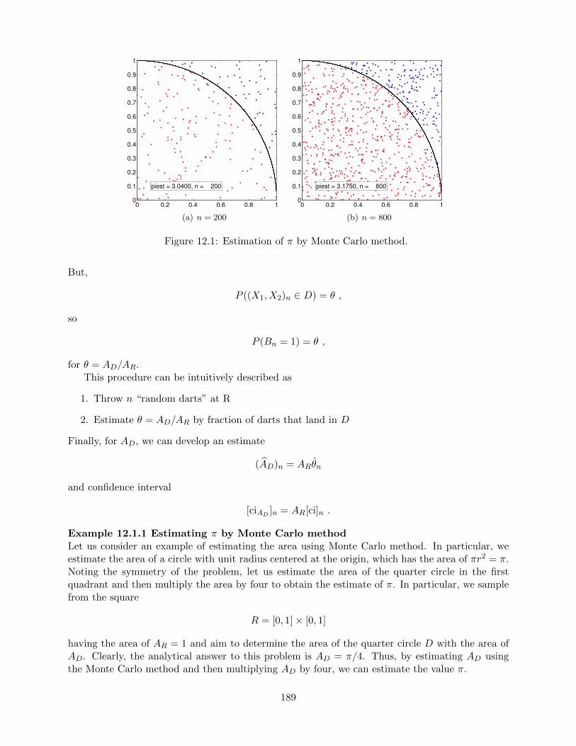
0 0.2 0.4 0.6 0.8 10

0.1

0.2

0.3

0.4

0.5

0.6

0.7

0.8

0.9

1

piest = 3.0400, n = 200

(a) n = 200

0 0.2 0.4 0.6 0.8 10

0.1

0.2

0.3

0.4

0.5

0.6

0.7

0.8

0.9

1

piest = 3.1750, n = 800

(b) n = 800

Figure 12.1: Estimation of π by Monte Carlo method.

But,

P ((X1, X2)n ∈ D) = θ ,

so

P (Bn = 1) = θ ,

for θ = AD/AR.This procedure can be intuitively described as

1. Throw n “random darts” at R

2. Estimate θ = AD/AR by fraction of darts that land in D

Finally, for AD, we can develop an estimate

(AD)n = ARθn

and confidence interval

[ciAD ]n = AR[ci]n .

Example 12.1.1 Estimating π by Monte Carlo methodLet us consider an example of estimating the area using Monte Carlo method. In particular, weestimate the area of a circle with unit radius centered at the origin, which has the area of πr2 = π.Noting the symmetry of the problem, let us estimate the area of the quarter circle in the firstquadrant and then multiply the area by four to obtain the estimate of π. In particular, we samplefrom the square

R = [0, 1]× [0, 1]

having the area of AR = 1 and aim to determine the area of the quarter circle D with the area ofAD. Clearly, the analytical answer to this problem is AD = π/4. Thus, by estimating AD usingthe Monte Carlo method and then multiplying AD by four, we can estimate the value π.

189

100

102

104

106

2

2.5

3

3.5

4

4.5

n

π e

stim

ate

π estimate

π

95% ci

(a) value

100

102

104

106

10−4

10−2

100

n

err

or

π estimate

n−1/2

95% ci

(b) error

Figure 12.2: Convergence of the π estimate with the number of samples.

The sampling procedure is illustrated in Figure 12.1. To determine whether a given sample(x1, x2)n is in the quarter circle, we can compute its distance from the center and determine if thedistance is greater than unity, i.e. the Bernoulli variable is assigned according to

bn =

{1,

√x2

1 + x22 ≤ 1

0, otherwise.

The samples that evaluates to bn = 1 and 0 are plotted in red and blue, respectively. Because thesamples are drawn uniformly from the square, the fraction of red dots is equal to the fraction of thearea occupied by the quarter circle. We show in Figure 12.2 the convergence of the Monte Carloestimation: we observe the anticipated square-root behavior. Note in the remainder of this sectionwe shall use the more conventional N rather than n for sample size.

·

12.1.5 Estimation: Riemann Sum

As a comparison, let us also use the midpoint rule to find the area of a two-dimensional region D.We first note that the area of D is equal to the integral of a characteristic function

χ(x1, x2) =

{1, (x1, x2) ∈ D0, otherwise

,

over the domain of integration R that encloses D. For simplicity, we consider rectangular domainR = [a1, b1] × [a2, b2]. We discretize the domain into N/2 little rectangles, each with the widthof (b1 − a1)/

√N/2 and the height of (b2 − a2)/

√N/2. We further divide each rectangle into

two right triangles to obtain a triangulation of R. The area of each little triangle K is AK =(b1 − a1)(b2 − a2)/N . Application of the midpoint rule to integrate the characteristic functionyields

AD ≈ (ARieD )N =

∑K

AKχ(xc,K) =∑K

(b1 − a1)(b2 − a2)

Nχ(xc,K) ,

190

0 0.2 0.4 0.6 0.8 10

0.1

0.2

0.3

0.4

0.5

0.6

0.7

0.8

0.9

1

pi ~ 3.1600, N = 200

(a) N = 200

0 0.2 0.4 0.6 0.8 10

0.1

0.2

0.3

0.4

0.5

0.6

0.7

0.8

0.9

1

pi ~ 3.1300, N = 800

(b) N = 800

Figure 12.3: Estimation of π by deterministic Riemann sum.

where xc,K is the centroid (i.e. the midpoint) of the triangle. Noting that AR = (b1 − a1)(b2 − a2)and rearranging the equation, we obtain

(ARieD )N = AR

1

N

∑K

χ(xc,K) .

Because the characteristic function takes on either 0 or 1, the summation is simply equal to thenumber of times that xc,K is in the region D. Thus, we obtain our final expression

(ARieD )NAR

=number of points in D

N.

Note that the expression is very similar to that of the Monte Carlo integration. The main differenceis that the sampling points are structured for the Riemann sum (i.e. the centroid of the triangles).

We can also estimate the error incurred in this process. First, we note that we cannot directlyapply the error convergence result for the midpoint rule developed previously because the derivationrelied on the smoothness of the integrand. The characteristic function is discontinuous along theboundary of D and thus is not smooth. To estimate the error, for simplicity, let us assume thedomain size is the same in each dimension, i.e. a = a1 = a2 and b = b1 = b2. Then, the area ofeach square is

h2 = (b− a)2/N .

Then,

(ARieD )N = (number of points in D) · h2 .

There are no errors created by little squares fully inside or fully outside D. All the error is due tothe squares that intersect the perimeter. Thus, the error bound can be expressed as

error ≈ (number of squares that intersect D) · h2 ≈ (PerimeterD/h) · h2

= O(h) = O(√AR/N) .

191

100

102

104

106

2.6

2.8

3

3.2

3.4

3.6

3.8

4

N

π e

stim

ate

π est. (MC)

π est. (RM)

π

(a) value

100

102

104

106

10−4

10−2

100

N

err

or

π est. (MC)

π est. (RM)

N−1/2

(b) error

Figure 12.4: Convergence of the π estimate with the number of samples using Riemann sum.

Note that this is an example of a priori error estimate. In particular, unlike the error estimatebased on the confidence interval of the sample mean for Monte Carlo, this estimate is not constant-free. That is, while we know the asymptotic rate at which the method converges, it does not tell usthe actual magnitude of the error, which is problem-dependent. A constant-free estimate typicallyrequires an a posteriori error estimate, which incorporates the information gathered about theparticular problem of interest. We show in Figure 12.3 the Riemann sum grid, and in Figure 12.4the convergence of the Riemann sum approach compared to the convergence of the Monte Carloapproach for our π example.

Example 12.1.2 Integration of a rectangular areaIn the case of finding the area of a quarter circle, the Riemann sum performed noticeably betterthan the Monte Carlo method. However, this is not true in general. To demonstrate this, let usconsider integrating the area of a rectangle. In particular, we consider the region

D = [0.2, 0.7]× [0.2, 0.8] .

The area of the rectangle is AD = (0.7− 0.2) · (0.8− 0.2) = 0.3.The Monte Carlo integration procedure applied to the rectangular area is illustrated in Fig-

ure 12.5(a). The convergence result in Figure 12.5(b) confirms that both Monte Carlo and Riemannsum converge at the rate of N−1/2. Moreover, both methods produce the error of similar level forall ranges of the sample size N considered.

·

Example 12.1.3 Integration of a complex areaLet us consider estimating the area of a more complex region, shown in Figure 12.6(a). The regionD is implicitly defined in the polar coordinate as

D =

{(r, θ) : r ≤ 2

3+

1

3cos(4βθ), 0 ≤ θ ≤ π

2

},

where r =√x2 + y2 and tan(θ) = y/x. The particular case shown in the figure is for β = 10. For

any natural number β, the area of the region D is equal to

AD =

∫ π/2

θ=0

∫ 2/3+1/3 cos(4βθ)

r=0r dr dθ =

π

8, β = 1, 2, . . . .

192

0 0.2 0.4 0.6 0.8 10

0.1

0.2

0.3

0.4

0.5

0.6

0.7

0.8

0.9

1

Area ~ 0.2875, N = 800

(a) Monte Carlo example

100

102

104

106

10−4

10−2

100

N

err

or

area est. (MC)

area est. (RM)

N−1/2

(b) error

Figure 12.5: The geometry and error convergence for the integration over a rectangular area.

0 0.2 0.4 0.6 0.8 10

0.1

0.2

0.3

0.4

0.5

0.6

0.7

0.8

0.9

1

pi ~ 3.1000, N = 800

(a) Monte Carlo example

100

102

104

106

10−4

10−2

100

N

err

or

π est. (MC)

π est. (RM)

N−1/2

(b) error

Figure 12.6: The geometry and error convergence for the integration over a more complex area.

Thus, we can again estimate π by multiplying the estimated area of D by 8.The result of estimating π by approximating the area of D is shown in Figure 12.6(b). The

error convergence plot confirms that both Monte Carlo and Riemann sum converge at the rate ofN−1/2. In fact, their performances are comparable for this slightly more complex domain.

·

12.2 Calculation of Volumes in Higher Dimensions

12.2.1 Three Dimensions

Both the Monte Carlo method and Riemann sum used to estimate the area of region D in twodimensions trivially extends to higher dimensions. Let us consider their applications in threedimensions.

193

Monte Carlo

Now, we sample (X1, X2, X3) uniformly from a parallelepiped R = [a1, b1]× [a2, b2]× [a3, b3], wherethe Xi’s are mutually independent. Then, we assign a Bernoulli random variable according towhether (X1, X2, X3) is inside or outside D as before, i.e.

B =

{1, (X1, X2, X3) ∈ D0, otherwise

.

Recall that the convergence of the sample mean to the true value — in particular the convergenceof the confidence interval — is related to the Bernoulli random variable and not the Xi’s. Thus,even in three dimensions, we still expect the error to converge as N−1/2, where N is the size of thesample.

Riemann Sum

For simplicity, let us assume the parallelepiped is a cube, i.e. a = a1 = a2 = a3 and b = b1 = b2 = b3.We consider a grid of N points centered in little cubes of size

h3 =b− aN

,

such that Nh3 = VR. Extending the two-dimensional case, we estimate the volume of the region Daccording to

V RieD

VR=

number of points in D

N.

However, unlike the Monte Carlo method, the error calculation is dependent on the dimension.The error is given by

error ≈ (number of cubes that intersect D) · h3

≈ (surface area of D/h2) · h3

≈ h ≈ N−1/3 .

Note that the convergence rate has decreased from N−1/2 to N−1/3 in going from two to threedimensions.

Example 12.2.1 Integration of a sphereLet us consider a problem of finding the volume of a unit 1/8th sphere lying in the first octant. Wesample from a unit cube

R = [0, 1]× [0, 1]× [0, 1]

having a volume of VR = 1.0. As in the case of circle in two dimensions, we can perform simplein/out check by measuring the distance of the point from the origin; i.e the Bernoulli variable isassigned according to

bn =

{1,

√x2

1 + x22 + x2

3 ≤ 1

0, otherwise.

The result of estimating the value of π based on the estimate of the volume of the 1/8th sphere isshown in Figure 12.7. (The raw estimated volume of the 1/8th sphere is scaled by 6.) As expected

194

100

101

102

103

104

105

106

2.5

3

3.5

4

4.5

5

5.5

6

N

π e

stim

ate

π est. (MC)

π est. (RM)

π

(a) value

100

101

102

103

104

105

106

10−4

10−2

100

N

err

or

π est. (MC)

π est. (RM)

N−1/2

N−1/3

(b) error

Figure 12.7: Convergence of the π estimate using the volume of a sphere.

both the Monte Carlo method and the Riemann sum converge to the correct value. In particular,the Monte Carlo method converges at the expected rate of N−1/2. The Riemann sum, on the otherhand, converges at a faster rate than the expected rate of N−1/3. This superconvergence is dueto the symmetry in the tetrahedralization used in integration and the volume of interest. Thisdoes not contradict our a priori analysis, because the analysis tells us the asymptotic convergencerate for the worst case. The following example shows that the asymptotic convergence rate of theRiemann sum for a general geometry is indeed N−1/2.

·

Example 12.2.2 Integration of a parallelpipedLet us consider a simpler example of finding the volume of a parallelpiped described by

D = [0.1, 0.9]× [0.2, 0.7]× [0.1, 0.8] .

The volume of the parallelpiped is VD = 0.28.Figure 12.8 shows the result of the integration. The figure shows that the convergence rate of

the Riemann sum is N−1/3, which is consistent with the a priori analysis. On the other hand, theMonte Carlo method performs just as well as it did in two dimension, converging at the rate ofN−1/2. In particular, the Monte Carlo method performs noticeably better than the Riemann sumfor large values of N .

·

Example 12.2.3 Integration of a complex volumeLet us consider a more general geometry, with the domain defined in the spherical coordinate as

D =

{(r, θ, φ) : r ≤ sin(θ)

(2

3+

1

3cos(40φ)

), 0 ≤ θ ≤ π

2, 0 ≤ φ ≤ π

2

}.

The volume of the region is given by

VD =

∫ π/2

φ=0

∫ π/2

θ=0

∫ sin(θ)( 23

+ 13

cos(40φ))

r=0r2 sin(θ) dr dθ dφ =

88

2835π .

195

100

102

104

106

0

0.1

0.2

0.3

0.4

0.5

0.6

N

vo

lum

e e

stim

ate

vol est. (MC)

vol est. (RM)

vol

(a) value

100

102

104

106

10−4

10−2

100

N

err

or

vol est. (MC)

vol est. (RM)

N−1/2

N−1/3

(b) error

Figure 12.8: Area of a parallelepiped.

100

101

102

103

104

105

106

0

5

10

15

20

25

N

π e

stim

ate

π est. (MC)

π est. (RM)

π

(a) value

100

101

102

103

104

105

106

10−4

10−2

100

N

err

or

π est. (MC)

π est. (RM)

N−1/2

N−1/3

(b) error

Figure 12.9: Convergence of the π estimate using a complex three-dimensional integration.

196

Thus, we can estimate the value of π by first estimating the volume using Monte Carlo or Riemannsum, and then multiplying the result by 2835/88.

Figure 12.9 shows the result of performing the integration. The figure shows that the conver-gence rate of the Riemann sum is N−1/3, which is consistent with the a priori analysis. On theother hand, the Monte Carlo method performs just as well as it did for the simple sphere case.

·

12.2.2 General d-Dimensions

Let us generalize our analysis to the case of integrating a general d-dimensional region. In this case,the Monte Carlo method considers a random d-vector, (X1, . . . , Xd), and associate with the vectora Bernoulli random variable. The convergence of the Monte Carlo integration is dependent onthe Bernoulli random variables and not directly affected by the random vector. In particular, theMonte Carlo method is oblivious to the length of the vector, d, i.e. the dimensionality of the space.Because the standard deviation of the binomial distribution scales as N−1/2, we still expect theMonte Carlo method to converge at the rate of N−1/2 regardless of d. Thus, Monte Carlo methodsdo not suffer from so-called curse of dimensionality, in which a method becomes intractable withincrease of the dimension of the problem.

On the other hand, the performance of the Riemann sum is a function of the dimension of the

space. In a d-dimensional space, each little cube has the volume of N−1, and there are Nd−1d cube

that intersect the boundary of D. Thus, the error scales as

error ≈ N d−1d N−1 = N−1/d .

The convergence rate worsens with the dimension, and this is an example of the curse of dimen-sionality. While the integration of a physical volume is typically limited to three dimensions, thereare many instances in science and engineering where a higher-dimensional integration is required.

Example 12.2.4 integration over a hypersphereTo demonstrate that the convergence of Monte Carlo method is independent of the dimension, letus consider integration of a hypersphere in d-dimensional space. The volume of d-sphere is givenby

VD =πd/2

Γ(n/2 + 1)rd ,

where Γ is the gamma function. We can again use the integration of a d-sphere to estimate thevalue of π.

The result of estimating the d-dimensional volume is shown in Figure 12.10 for d = 2, 3, 5, 7.The error convergence plot shows that the method converges at the rate of N−1/2 for all d. Theresult confirms that Monte Carlo integration is a powerful method for integrating functions inhigher-dimensional spaces.

·

197

100

102

104

106

0

0.5

1

1.5

2

2.5

3

3.5

4

4.5

N

π e

stim

ate

d = 2

d = 3

d = 5

d = 7

(a) value

100

102

104

106

10−4

10−3

10−2

10−1

100

101

N

err

or

d = 2

d = 3

d = 5

d = 7

N−1/2

(b) error

Figure 12.10: Convergence of the π estimate using the Monte Carlo method on d-dimensionalhyperspheres.

198

Chapter 13

Monte Carlo: General IntegrationProcedures

199

DRAFT V2.1 © The Authors. License: Creative Commons BY-NC-SA 3.0.

200

Chapter 14

Monte Carlo: Failure Probabilities

14.1 Calculating a Failure Probability

14.1.1 Objective

Let’s say there is a set of “environmental” or “load” variables (x1, x2, . . . ) that affect the perfor-mance of an engineering system. For simplicity, let us restrict ourselves to the parameter size oftwo, so that we only have (x1, x2). We also assume that there are two “performance” metrics,g1(x1, x2) and g2(x1, x2). Without loss of generality, let’s assume smaller g1 and g2 means betterperformance (we can always consider negative of the performance variable if larger values implybetter performance). In fact, we assume that we wish to confirm that the performance metrics arebelow certain thresholds, i.e.

g1(x1, x2) ≤ τ1 and g2(x1, x2) ≤ τ2 . (14.1)

Equivalently, we wish to avoid failure, which is defined as

g1(x1, x2) > τ1 or g2(x1, x2) > τ2 .

Note that in this chapter failure is interpreted liberally as the condition (14.1) even if this conditionis not equivalent in any given situation as actual failure.

Suppose that (x1, x2) reside in some rectangle R. We now choose to interpret (x1, x2) as realiza-tions of a random vector X = (X1, X2) with prescribed probability density function fX(x1, x2) =fX1,X2(x1, x2). We then wish to quantify the failure probability θF , defined by

θF = P (g1(X1, X2) > τ1 or g2(X1, X2) > τ2) .

We note that g1 and g2 are deterministic functions; however, because the argument to the functionsare random variables, the output g1(X1, X2) and g2(X1, X2) are random variables. Thus, the failureis described probabilistically. If the bounds on the environmental variables (x1, x2) are known apriori one could design a system to handle the worst possible cases; however, the system design tohandle very rare events may be over designed. Thus, a probabilistic approach may be appropriatein many engineering scenarios.

In any probabilistic simulation, we must make sure that the probability density of the randomvariable, fX , is meaningful and that the interpretation of the probabilistic statement is relevant.

201

DRAFT V2.1 © The Authors. License: Creative Commons BY-NC-SA 3.0.

For example, in constructing the distribution, a good estimate may be obtained from statisticaldata (i.e. by sampling a population). The failure probability θF can be interpreted as either(i) probability of failure for the next “random” set of environmental or operating conditions, or(ii) frequency of failure over a population (based on the frequentist perspective).

14.1.2 An Integral

We now show that the computation of failure probability is similar to computation of an area. Letus define R to be the region from which X = (X1, X2) is sampled (not necessarily uniformly). Inother words, R encompasses all possible values that the environmental variable X can take. Let usalso define D to be the region whose element (x1, x2) ∈ D would lead to failure, i.e.

D ≡ {(x1, x2) : g1(x1, x2) > τ1 or g2(x1, x2) > τ2} .

Then, the failure probability can be expressed as an integral

θF =

∫∫DfX(x1, x2)dx1dx2 .

This requires a integration over the region D, which can be complicated depending on the failurecriteria.

However, we can simplify the integral using the technique previously used to compute the area.Namely, we introduce a failure indicator or characteristic function,

1F (x1, x2) =

{1, g1(x1, x2) > τ1 or g2(x1, x2) > τ2

0, otherwise.

Using the failure indicator, we can write the integral over D as an integral over the simpler domainR, i.e.

θF =

∫∫R

1(x1, x2)fX(x1, x2) dx1 dx2 .

Note that Monte Carlo methods can be used to evaluate any integral in any number of dimensions.The two main approaches are “hit or miss” and “sample mean,” with the latter more efficient. Ourcase here is a natural example of the sample mean approach, though it also has the flavor of “hitor miss.” In practice, variance reduction techniques are often applied to improve the convergence.

14.1.3 A Monte Carlo Approach

We can easily develop a Monte Carlo approach if we can reduce our problem to a Bernoulli randomvariable with parameter θF such that

B =

{1, with probability θF

0, with probability 1− θF.

Then, the computation of the failure probability θF becomes the estimation of parameter θF throughsampling (as in the coin flip example). This is easy: we draw a random vector (X1, X2) from fX— for example, uniform or normal — and then define

B =

{1, g1(X) > τ1 or g2(X) > τ2

0, otherwise. (14.2)

202

Determination of B is easy assuming we can evaluate g1(x1, x2) and g2(x1, x2). But, by definition

θF = P (g1(X) > τ1 or g2(X) > τ2)

=

∫∫R

1F (x1, x2)fX(x1, x2) dx1 dx2 .

Hence we have identified a Bernoulli random variable with the requisite parameter θF .The Monte Carlo procedure is simple. First, we draw nmax random variables,

(X1, X2)1, (X1, X2)2, . . . , (X1, X2)n, . . . , (X1, X2)nmax ,

and map them to Bernoulli random variables

(X1, X2)n → Bn n = 1, . . . , nmax ,

according to (14.2). Using this mapping, we assign sample means, Θn, and confidence intervals,[CIF ]n, according to

(ΘF )n =1

n

n∑i=1

Bi , (14.3)

[CIF ]n =

(ΘF )n − zγ

√(ΘF )n(1− (ΘF )n)

n, (ΘF )n + zγ

√(ΘF )n(1− (ΘF )n)

n

. (14.4)

Note that in cases of failure, typically we would like θF to be very small. We recall from Sec-tion 10.3.3 that it is precisely this case for which the relative error RelErr is quite large (andfurthermore for which the normal density confidence interval is only valid for quite large n). Hence,in practice, we must consider very large sample sizes in order to obtain relatively accurate resultswith reasonable confidence. More sophisticated approaches partially address these issues, but eventhese advanced approaches often rely on basic Monte Carlo ingredients.

Finally, we note that although the above description is for the cumulative approach we can alsodirectly apply equations 14.3 and 14.4 for any fixed n. In this case we obtain Pr(θF ∈ [CIf ]n) = γ.

203

204

Unit III

Linear Algebra 1: Matrices and LeastSquares. Regression.

205

Chapter 15

Motivation

In odometry-based mobile robot navigation, the accuracy of the robot’s dead reckoning posetracking depends on minimizing slippage between the robot’s wheels and the ground. Even amomentary slip can lead to an error in heading that will cause the error in the robot’s locationestimate to grow linearly over its journey. It is thus important to determine the friction coefficientbetween the robot’s wheels and the ground, which directly affects the robot’s resistance to slippage.Just as importantly, this friction coefficient will significantly affect the performance of the robot:the ability to push loads.

When the mobile robot of Figure 15.1 is commanded to move forward, a number of forces comeinto play. Internally, the drive motors exert a torque (not shown in the figure) on the wheels,which is resisted by the friction force Ff between the wheels and the ground. If the magnitude of Ff

dictated by the sum of the drag force Fdrag (a combination of all forces resisting the robot’s motion)and the product of the robot’s mass and acceleration is less than the maximum static friction forceFmax

f, static between the wheels and the ground, the wheels will roll without slipping and the robotwill move forward with velocity v = ωrwheel. If, however, the magnitude of Ff reaches Fmax

f, static, thewheels will begin to slip and Ff will drop to a lower level Ff, kinetic, the kinetic friction force. Thewheels will continue to slip (v < ωrwheel) until zero relative motion between the wheels and theground is restored (when v = ωrwheel).

The critical value defining the boundary between rolling and slipping, therefore, is the maximum

Fnormal, front Fnormal, rear

w

F f

v

Fdrag

W

Figure 15.1: A mobile robot in motion.

207

DRAFT V2.1 © The Authors. License: Creative Commons BY-NC-SA 3.0.

Figure 15.2: Experimental setup for frictionmeasurement: Force transducer (A) is con-nected to contact area (B) by a thin wire.Normal force is exerted on the contact areaby load stack (C). Tangential force is ap-plied using turntable (D) via the friction be-tween the turntable surface and the contactarea. Apparatus and photograph courtesy ofJames Penn.

0 1 2 3 4 5 6 7 80.10.20.30.40.50.60.70.80.9

time (seconds)

time (seconds)

F

F

friction

friction

vs.

vs. Tim

Time

e for

for 500

500 Gr

Gram

am Load

Load

F

F

f

f,

, ki

kine

net

tic

ic

=

= µ

µ

k

k

F

F

nor

norma

mal

l

+

+ exp

experi

erim

men

ental

tal error

error

F F

fric

tion

fric

tion

(New

tons

)

(New

tons

)

F

F

f

f,

, stat

static

ic

=

= F

F

ta

tangen

ngent

tia

ial

l,, appl

applied

ied

≤

≤ µ

µ

s

s

F

F

nor

norma

mal

l

m

measeas

=

= µ

µ

s

s

F

F

nor

norma

mal

l

+

+ exp

expe

eri

rim

men

ental

tal error

errorF

F

f

f,

, stat

static

icm

max,ax,

meas

meas

Figure 15.3: Sample data for one frictionmeasurement, yielding one data point forFmax,meas

f, static . Data courtesy of James Penn.

static friction force. We expect that

Fmaxf, static = µs Fnormal, rear , (15.1)

where µs is the static coefficient of friction and Fnormal, rear is the normal force from the ground onthe rear, driving, wheels. In order to minimize the risk of slippage (and to be able to push largeloads), robot wheels should be designed for a high value of µs between the wheels and the ground.This value, although difficult to predict accurately by modeling, can be determined by experiment.

We first conduct experiments for the friction force Fmaxf, static (in Newtons) as a function of normal

load Fnormal, applied (in Newtons) and (nominal) surface area of contact Asurface (in cm2) with thefriction turntable apparatus depicted in Figure 15.2. Weights permit us to vary the normal load and“washer” inserts permit us to vary the nominal surface area of contact. A typical experiment (at aparticular prescribed value of Fnormal, applied and Asurface) yields the time trace of Figure 15.3 fromwhich the Fmax,means

f, static (our measurement of Fmaxf, static) is deduced as the maximum of the response.

We next postulate a dependence (or “model”)

Fmaxf, static(Fnormal, applied, Asurface) = β0 + β1 Fnormal, applied + β2 Asurface , (15.2)

where we expect — but do not a priori assume — from Messieurs Amontons and Coulomb thatβ0 = 0 and β2 = 0 (and of course β1 ≡ µs). In order to confirm that β0 = 0 and β2 = 0 — or atleast confirm that β0 = 0 and β2 = 0 is not untrue — and to find a good estimate for β1 ≡ µs, wemust appeal to our measurements.

The mathematical techniques by which to determine µs (and β0, β2) “with some confidence”from noisy experimental data is known as regression, which is the subject of Chapter 19. Regression,in turn, is best described in the language of linear algebra (Chapter 16), and is built upon the linearalgebra concept of least squares (Chapter 17).

208

Chapter 16

Matrices and Vectors: Definitions andOperations

16.1 Basic Vector and Matrix Operations

16.1.1 Definitions

Let us first introduce the primitive objects in linear algebra: vectors and matrices. A m-vectorv ∈ Rm×1 consists of m real numbers 1

v =

v1

v2...vm

.

It is also called a column vector, which is the default vector in linear algebra. Thus, by convention,v ∈ Rm implies that v is a column vector in Rm×1. Note that we use subscript (·)i to address thei-th component of a vector. The other kind of vector is a row vector v ∈ R1×n consisting of nentries

v =(v1 v2 · · · vn

).

Let us consider a few examples of column and row vectors.

Example 16.1.1 vectorsExamples of (column) vectors in R3 are

v =

136

, u =

√

3−7π

, and w =

9.17/3√π

.

1The concept of vectors readily extends to complex numbers, but we only consider real vectors in our presentationof this chapter.

209

DRAFT V2.1 © The Authors. License: Creative Commons BY-NC-SA 3.0.

To address a specific component of the vectors, we write, for example, v1 = 1, u1 =√

3, andw3 =

√π. Examples of row vectors in R1×4 are

v =(

2 −5√

2 e)

and u =(−√π 1 1 0

).

Some of the components of these row vectors are v2 = −5 and u4 = 0.

·A matrix A ∈ Rm×n consists of m rows and n columns for the total of m · n entries,

A =

A11 A12 · · · A1n

A21 A22 · · · A2n...

.... . .

...Am1 Am2 · · · Amn

.

Extending the convention for addressing an entry of a vector, we use subscript (·)ij to address theentry on the i-th row and j-th column. Note that the order in which the row and column arereferred follows that for describing the size of the matrix. Thus, A ∈ Rm×n consists of entries

Aij , i = 1, . . . ,m, j = 1, . . . , n .

Sometimes it is convenient to think of a (column) vector as a special case of a matrix with only onecolumn, i.e., n = 1. Similarly, a (row) vector can be thought of as a special case of a matrix withm = 1. Conversely, an m× n matrix can be viewed as m row n-vectors or n column m-vectors, aswe discuss further below.

Example 16.1.2 matricesExamples of matrices are

A =

1√

3−4 9π −3

and B =

0 0 1−2 8 10 3 0

.

The matrix A is a 3 × 2 matrix (A ∈ R3×2) and matrix B is a 3 × 3 matrix (B ∈ R3×3). We canalso address specific entries as, for example, A12 =

√3, A31 = −4, and B32 = 3.

·While vectors and matrices may appear like arrays of numbers, linear algebra defines special

set of rules to manipulate these objects. One such operation is the transpose operation considerednext.

Transpose Operation

The first linear algebra operator we consider is the transpose operator, denoted by superscript (·)T.The transpose operator swaps the rows and columns of the matrix. That is, if B = AT withA ∈ Rm×n, then

Bij = Aji, 1 ≤ i ≤ n, 1 ≤ j ≤ m .

Because the rows and columns of the matrix are swapped, the dimensions of the matrix are alsoswapped, i.e., if A ∈ Rm×n then B ∈ Rn×m.

If we swap the rows and columns twice, then we return to the original matrix. Thus, thetranspose of a transposed matrix is the original matrix, i.e.

(AT)T = A .

210

Example 16.1.3 transposeLet us consider a few examples of transpose operation. A matrix A and its transpose B = AT arerelated by

A =

1√

3−4 9π −3

and B =

(1 −4 π√3 9 −3

).

The rows and columns are swapped in the sense that A31 = B13 = π and A12 = B21 =√

3. Also,because A ∈ R3×2, B ∈ R2×3. Interpreting a vector as a special case of a matrix with one column,we can also apply the transpose operator to a column vector to create a row vector, i.e., given

v =

√

3−7π

,

the transpose operation yields

u = vT =( √

3 −7 π).

Note that the transpose of a column vector is a row vector, and the transpose of a row vector is acolumn vector.

·

16.1.2 Vector Operations

The first vector operation we consider is multiplication of a vector v ∈ Rm by a scalar α ∈ R. Theoperation yields

u = αv ,

where each entry of u ∈ Rm is given by

ui = αvi, i = 1, . . . ,m .

In other words, multiplication of a vector by a scalar results in each component of the vector beingscaled by the scalar.

The second operation we consider is addition of two vectors v ∈ Rm and w ∈ Rm. The additionyields

u = v + w ,

where each entry of u ∈ Rm is given by

ui = vi + wi, i = 1, . . . ,m .

In order for addition of two vectors to make sense, the vectors must have the same number ofcomponents. Each entry of the resulting vector is simply the sum of the corresponding entries ofthe two vectors.

We can summarize the action of the scaling and addition operations in a single operation. Letv ∈ Rm, w ∈ Rm and α ∈ R. Then, the operation

u = v + αw

211

0 0.5 1 1.50

0.5

1

1.5

v

u=α v

(a) scalar scaling

0 0.5 1 1.50

0.5

1

1.5

v

w

u=v+w

(b) vector addition

Figure 16.1: Illustration of vector scaling and vector addition.

yields a vector u ∈ Rm whose entries are given by

ui = vi + αwi, i = 1, . . . ,m .

The result is nothing more than a combination of the scalar multiplication and vector additionrules.

Example 16.1.4 vector scaling and addition in R2

Let us illustrate scaling of a vector by a scalar and addition of two vectors in R2 using

v =

(1

1/3

), w =

(1/21

), and α =

3

2.

First, let us consider scaling of the vector v by the scalar α. The operation yields

u = αv =3

2

(1

1/3

)=

(3/21/2

).

This operation is illustrated in Figure 16.1(a). The vector v is simply stretched by the factor of3/2 while preserving the direction.

Now, let us consider addition of the vectors v and w. The vector addition yields

u = v + w =

(1

1/3

)+

(1/21

)=

(3/24/3

).

Figure 16.1(b) illustrates the vector addition process. We translate w so that it starts from thetip of v to form a parallelogram. The resultant vector is precisely the sum of the two vectors.Note that the geometric intuition for scaling and addition provided for R2 readily extends to higherdimensions.

·

212

Example 16.1.5 vector scaling and addition in R3

Let v =(

1 3 6)T

, w =(

2 −1 0)T

, and α = 3. Then,

u = v + αw =

136

+ 3 ·

2−10

=

136

+

6−30

=

706

.

·

Inner Product

Another important operation is the inner product. This operation takes two vectors of the samedimension, v ∈ Rm and w ∈ Rm, and yields a scalar β ∈ R:

β = vTw where β =m∑i=1

viwi .

The appearance of the transpose operator will become obvious once we introduce the matrix-matrixmultiplication rule. The inner product in a Euclidean vector space is also commonly called the dotproduct and is denoted by β = v ·w. More generally, the inner product of two elements of a vectorspace is denoted by (·, ·), i.e., β = (v, w).

Example 16.1.6 inner product

Let us consider two vectors in R3, v =(

1 3 6)T

and w =(

2 −1 0)T

. The inner product

of these two vectors is

β = vTw =

3∑i=1

viwi = 1 · 2 + 3 · (−1) + 6 · 0 = −1 .

·

Norm (2-Norm)

Using the inner product, we can naturally define the 2-norm of a vector. Given v ∈ Rm, the 2-normof v, denoted by ‖v‖2, is defined by

‖v‖2 =√vTv =

√√√√ m∑i=1

v2i .

Note that the norm of any vector is non-negative, because it is a sum m non-negative numbers(squared values). The `2 norm is the usual Euclidean length; in particular, for m = 2, the expressionsimplifies to the familiar Pythagorean theorem, ‖v‖2 =

√v2

1 + v22. While there are other norms, we

almost exclusively use the 2-norm in this unit. Thus, for notational convenience, we will drop thesubscript 2 and write the 2-norm of v as ‖v‖ with the implicit understanding ‖ · ‖ ≡ ‖ · ‖2.

By definition, any norm must satisfy the triangle inequality,

‖v + w‖ ≤ ‖v‖+ ‖w‖ ,

213

for any v, w ∈ Rm. The theorem states that the sum of the lengths of two adjoining segmentsis longer than the distance between their non-joined end points, as is intuitively clear from Fig-ure 16.1(b). For norms defined by inner products, as our 2-norm above, the triangle inequality isautomatically satisfied.

Proof. For norms induced by an inner product, the proof of the triangle inequality follows directlyfrom the definition of the norm and the Cauchy-Schwarz inequality. First, we expand the expressionas

‖v + w‖2 = (v + w)T(v + w) = vTv + 2vTw + wTw .

The middle terms can be bounded by the Cauchy-Schwarz inequality, which states that

vTw ≤ |vTw| ≤ ‖v‖‖w‖ .

Thus, we can bound the norm as

‖v + w‖2 ≤ ‖v‖2 + 2‖v‖‖w‖+ ‖w‖2 = (‖v‖+ ‖w‖)2 ,

and taking the square root of both sides yields the desired result.

Example 16.1.7 norm of a vector

Let v =(

1 3 6)T

and w =(

2 −1 0)T

. The `2 norms of these vectors are

‖v‖ =

√√√√ 3∑i=1

v2i =

√12 + 32 + 62 =

√46

and ‖w‖ =

√√√√ 3∑i=1

w2i =

√22 + (−1)2 + 02 =

√5 .

·

Example 16.1.8 triangle inequalityLet us illustrate the triangle inequality using two vectors

v =

(1

1/3

)and w =

(1/21

).

The length (or the norm) of the vectors are

‖v‖ =

√10

9≈ 1.054 and ‖w‖ =

√5

4≈ 1.118 .

On the other hand, the sum of the two vectors is

v + w =

(1

1/3

)+

(1/21

)=

(3/24/3

),

214

0 0.5 1 1.50

0.5

1

1.5

v

w

v+w

||v||

||w||

Figure 16.2: Illustration of the triangle inequality.

and its length is

‖v + w‖ =

√145

6≈ 2.007 .

The norm of the sum is shorter than the sum of the norms, which is

‖v‖+ ‖w‖ ≈ 2.172 .

This inequality is illustrated in Figure 16.2. Clearly, the length of v+w is strictly less than the sumof the lengths of v and w (unless v and w align with each other, in which case we obtain equality).

·In two dimensions, the inner product can be interpreted as

vTw = ‖v‖‖w‖ cos(θ) , (16.1)

where θ is the angle between v and w. In other words, the inner product is a measure of how wellv and w align with each other. Note that we can show the Cauchy-Schwarz inequality from theabove equality. Namely, | cos(θ)| ≤ 1 implies that

|vTw| = ‖v‖‖w‖| cos(θ)| ≤ ‖v‖‖w‖ .

In particular, we see that the inequality holds with equality if and only if θ = 0 or π, whichcorresponds to the cases where v and w align. It is easy to demonstrate Eq. (16.1) in two dimensions.

Proof. Noting v, w ∈ R2, we express them in polar coordinates

v = ‖v‖(

cos(θv)sin(θv)

)and w = ‖w‖

(cos(θw)sin(θw)

).

215

The inner product of the two vectors yield

β = vTw =2∑i=1

viwi = ‖v‖ cos(θv)‖w‖ cos(θw) + ‖v‖ sin(θv)‖w‖ sin(θw)

= ‖v‖‖w‖(cos(θv) cos(θw) + sin(θv) sin(θw)

)= ‖v‖‖w‖

(1

2(eiθv + e−iθv)

1

2(eiθw + e−iθw) +

1

2i(eiθv − e−iθv) 1

2i(eiθw − e−iθw)

)= ‖v‖‖w‖

(1

4

(ei(θv+θw) + e−i(θv+θw) + ei(θv−θw) + e−i(θv−θw)

)−1

4

(ei(θv+θw) + e−i(θv+θw) − ei(θv−θw) − e−i(θv−θw)

))= ‖v‖‖w‖

(1

2

(ei(θv−θw) + e−i(θv−θw)

))= ‖v‖‖w‖ cos(θv − θw) = ‖v‖‖w‖ cos(θ) ,

where the last equality follows from the definition θ ≡ θv − θw.

Begin Advanced Material

For completeness, let us introduce a more general class of norms.

Example 16.1.9 p-normsThe 2-norm, which we will almost exclusively use, belong to a more general class of norms, calledthe p-norms. The p-norm of a vector v ∈ Rm is

‖v‖p =

m∑i=1

|vi|p1/p

,

where p ≥ 1. Any p-norm satisfies the positivity requirement, the scalar scaling requirement, andthe triangle inequality. We see that 2-norm is a case of p-norm with p = 2.

Another case of p-norm that we frequently encounter is the 1-norm, which is simply the sum ofthe absolute value of the entries, i.e.

‖v‖1 =

m∑i=1

|vi| .

The other one is the infinity norm given by

‖v‖∞ = limp→∞

‖v‖p = maxi=1,...,m

|vi| .

In other words, the infinity norm of a vector is its largest entry in absolute value.

·

End Advanced Material

216

−5 −4 −3 −2 −1 0 1 2 3 40

1

2

3

4

5

6

7

u

v

w

Figure 16.3: Set of vectors considered to illustrate orthogonality.

Orthogonality

Two vectors v ∈ Rm and w ∈ Rm are said to be orthogonal to each other if

vTw = 0 .

In two dimensions, it is easy to see that

vTw = ‖v‖‖w‖ cos(θ) = 0 ⇒ cos(θ) = 0 ⇒ θ = π/2 .

That is, the angle between v and w is π/2, which is the definition of orthogonality in the usualgeometric sense.

Example 16.1.10 orthogonalityLet us consider three vectors in R2,

u =

(−42

), v =

(36

), and w =

(05

),

and compute three inner products formed by these vectors:

uTv = −4 · 3 + 2 · 6 = 0

uTw = −4 · 0 + 2 · 5 = 10

vTw = 3 · 0 + 6 · 5 = 30 .

Because uTv = 0, the vectors u and v are orthogonal to each other. On the other hand, uTw 6= 0and the vectors u and w are not orthogonal to each other. Similarly, v and w are not orthogonal toeach other. These vectors are plotted in Figure 16.3; the figure confirms that u and v are orthogonalin the usual geometric sense.

·

217

−1 −0.5 0 0.5 10

0.5

1

u

v

Figure 16.4: An orthonormal set of vectors.

Orthonormality

Two vectors v ∈ Rm and w ∈ Rm are said to be orthonormal to each other if they are orthogonalto each other and each has unit length, i.e.

vTw = 0 and ‖v‖ = ‖w‖ = 1 .

Example 16.1.11 orthonormalityTwo vectors

u =1√5

(−21

)and v =

1√5

(12

)are orthonormal to each other. It is straightforward to verify that they are orthogonal to each other

uTv =1√5

(−21

)T1√5

(12

)=

1

5

(−21

)T(12

)= 0

and that each of them have unit length

‖u‖ =

√1

5((−2)2 + 12) = 1

‖v‖ =

√1

5((1)2 + 22) = 1 .

Figure 16.4 shows that the vectors are orthogonal and have unit length in the usual geometricsense.

·

16.1.3 Linear Combinations

Let us consider a set of n m-vectors

v1 ∈ Rm, v2 ∈ Rm, . . . , vn ∈ Rm .

A linear combination of the vectors is given by

w =n∑j=1

αjvj ,

where α1, α2, . . . , αn is a set of real numbers, and each vj is an m-vector.

218

Example 16.1.12 linear combination of vectors

Let us consider three vectors in R2, v1 =(−4 2

)T, v2 =

(3 6

)T, and v3 =

(0 5

)T. A

linear combination of the vectors, with α1 = 1, α2 = −2, and α3 = 3, is

w =

3∑j=1

αjvj = 1 ·(−42

)+ (−2) ·

(36

)+ 3 ·

(05

)

=

(−42

)+

(−6−12

)+

(015

)=

(−10

5

).

Another example of linear combination, with α1 = 1, α2 = 0, and α3 = 0, is

w =3∑j=1

αjvj = 1 ·(−42

)+ 0 ·

(36

)+ 0 ·

(05

)=

(−42

).

Note that a linear combination of a set of vectors is simply a weighted sum of the vectors.

·

Linear Independence

A set of n m-vectors are linearly independent if

n∑j=1

αjvj = 0 only if α1 = α2 = · · · = αn = 0 .

Otherwise, the vectors are linearly dependent.

Example 16.1.13 linear independenceLet us consider four vectors,

w1 =

200

, w2 =

003

, w3 =

010

, and w4 =

205

.

The set of vectors {w1, w2, w4} is linearly dependent because

1 · w1 +5

3· w2 − 1 · w4 = 1 ·

200

+5

3·

003

− 1 ·

205

=

000

;

the linear combination with the weights {1, 5/3,−1} produces the zero vector. Note that the choiceof the weights that achieves this is not unique; we just need to find one set of weights to show thatthe vectors are not linearly independent (i.e., are linearly dependent).

On the other hand, the set of vectors {w1, w2, w3} is linearly independent. Considering a linearcombination,

α1w1 + α2w2 + α3w3 = α1 ·

200

+ α2 ·

003

+ α3 ·

010

=

000

,

219

we see that we must choose α1 = 0 to set the first component to 0, α2 = 0 to set the thirdcomponent to 0, and α3 = 0 to set the second component to 0. Thus, only way to satisfy theequation is to choose the trivial set of weights, {0, 0, 0}. Thus, the set of vectors {w1, w2, w3} islinearly independent.

·Begin Advanced Material

Vector Spaces and Bases

Given a set of n m-vectors, we can construct a vector space, V , given by

V = span({v1, v2, . . . , vn}) ,

where

span({v1, v2, . . . , vn}) =

v ∈ Rm : v =n∑k=1

αkvk, αk ∈ Rn

= space of vectors which are linear combinations of v1, v2, . . . , vn .

In general we do not require the vectors {v1, . . . , vn} to be linearly independent. When they arelinearly independent, they are said to be a basis of the space. In other words, a basis of the vectorspace V is a set of linearly independent vectors that spans the space. As we will see shortly in ourexample, there are many bases for any space. However, the number of vectors in any bases for agiven space is unique, and that number is called the dimension of the space. Let us demonstratethe idea in a simple example.

Example 16.1.14 Bases for a vector space in R3

Let us consider a vector space V spanned by vectors

v1 =

120

v2 =

210

and v3 =

010

.

By definition, any vector x ∈ V is of the form

x = α1v1 + α2v2 + α3v3 = α1

120

+ α2

210

+ α3

010

=

α1 + 2α2

2α1 + α2 + α3

0

.

Clearly, we can express any vector of the form x = (x1, x2, 0)T by choosing the coefficients α1,α2, and α3 judiciously. Thus, our vector space consists of vectors of the form (x1, x2, 0)T, i.e., allvectors in R3 with zero in the third entry.

We also note that the selection of coefficients that achieves (x1, x2, 0)T is not unique, as itrequires solution to a system of two linear equations with three unknowns. The non-uniqueness ofthe coefficients is a direct consequence of {v1, v2, v3} not being linearly independent. We can easilyverify the linear dependence by considering a non-trivial linear combination such as

2v1 − v2 − 3v3 = 2 ·

120

− 1 ·

210

− 3 ·

010

=

000

.

220

Because the vectors are not linearly independent, they do not form a basis of the space.To choose a basis for the space, we first note that vectors in the space V are of the form

(x1, x2, 0)T. We observe that, for example,

w1 =

100

and w2 =

010

would span the space because any vector in V — a vector of the form (x1, x2, 0)T — can be expressedas a linear combination, x1

x2

0

= α1w1 + α2w2 = α1

100

+ α2

001

=

α1

α2

0

,

by choosing α1 = x1 and α2 = x2. Moreover, w1 and w2 are linearly independent. Thus, {w1, w2} isa basis for the space V . Unlike the set {v1, v2, v3} which is not a basis, the coefficients for {w1, w2}that yields x ∈ V is unique. Because the basis consists of two vectors, the dimension of V is two.This is succinctly written as

dim(V ) = 2 .

Because a basis for a given space is not unique, we can pick a different set of vectors. Forexample,

z1 =

120

and z2 =

210

,

is also a basis for V . Since z1 is not a constant multiple of z2, it is clear that they are linearlyindependent. We need to verify that they span the space V . We can verify this by a directargument, x1

x2

0

= α1z1 + α2z2 = α1

120

+ α2

210

=

α1 + 2α2

2α1 + α2

0

.

We see that, for any (x1, x2, 0)T, we can find the linear combination of z1 and z2 by choosing thecoefficients α1 = (−x1 + 2x2)/3 and α2 = (2x1 − x2)/3. Again, the coefficients that represents xusing {z1, z2} are unique.

For the space V , and for any given basis, we can find a unique set of two coefficients to representany vector x ∈ V . In other words, any vector in V is uniquely described by two coefficients, orparameters. Thus, a basis provides a parameterization of the vector space V . The dimension of thespace is two, because the basis has two vectors, i.e., the vectors in the space are uniquely describedby two parameters.

·While there are many bases for any space, there are certain bases that are more convenient to

work with than others. Orthonormal bases — bases consisting of orthonormal sets of vectors —are such a class of bases. We recall that two set of vectors are orthogonal to each other if their

221

inner product vanishes. In order for a set of vectors {v1, . . . , vn} to be orthogonal, the vectors mustsatisfy

(vi)Tvj = 0, i 6= j .

In other words, the vectors are mutually orthogonal. An orthonormal set of vectors is an orthogonalset of vectors with each vector having norm unity. That is, the set of vectors {v1, . . . , vn} is mutuallyorthonormal if

(vi)Tvj = 0, i 6= j

‖vi‖ = (vi)Tvi = 1, i = 1, . . . , n .

We note that an orthonormal set of vectors is linearly independent by construction, as we nowprove.

Proof. Let {v1, . . . , vn} be an orthogonal set of (non-zero) vectors. By definition, the set of vectorsis linearly independent if the only linear combination that yields the zero vector corresponds to allcoefficients equal to zero, i.e.

α1v1 + · · ·+ αnvn = 0 ⇒ α1 = · · · = αn = 0 .

To verify this indeed is the case for any orthogonal set of vectors, we perform the inner product ofthe linear combination with v1, . . . , vn to obtain

(vi)T(α1v1 + · · ·+ αnvn) = α1(vi)Tv1 + · · ·+ αi(vi)Tvi + · · ·+ αn(vi)Tvn

= αi‖vi‖2, i = 1, . . . , n .

Note that (vi)Tvj = 0, i 6= j, due to orthogonality. Thus, setting the linear combination equal tozero requires

αi‖vi‖2 = 0, i = 1, . . . , n .

In other words, αi = 0 or ‖vi‖2 = 0 for each i. If we restrict ourselves to a set of non-zero vectors,then we must have αi = 0. Thus, a vanishing linear combination requires α1 = · · · = αn = 0, whichis the definition of linear independence.

Because an orthogonal set of vectors is linearly independent by construction, an orthonormalbasis for a space V is an orthonormal set of vectors that spans V . One advantage of using anorthonormal basis is that finding the coefficients for any vector in V is straightforward. Suppose,we have a basis {v1, . . . , vn} and wish to find the coefficients α1, . . . , αn that results in x ∈ V . Thatis, we are looking for the coefficients such that

x = α1v1 + · · ·+ αivi + · · ·+ αnvn .

To find the i-th coefficient αi, we simply consider the inner product with vi, i.e.

(vi)Tx = (vi)T(α1v1 + · · ·+ αivi + · · ·+ αnvn)

= α1(vi)Tv1 + · · ·+ αi(vi)Tvi + · · ·+ αn(vi)Tvn

= αi(vi)Tvi = αi‖vi‖2 = αi, i = 1, . . . , n ,

where the last equality follows from ‖vi‖2 = 1. That is, αi = (vi)Tx, i = 1, . . . , n. In particular, foran orthonormal basis, we simply need to perform n inner products to find the n coefficients. Thisis in contrast to an arbitrary basis, which requires a solution to an n × n linear system (which issignificantly more costly, as we will see later).

222

Example 16.1.15 Orthonormal BasisLet us consider the space vector space V spanned by

v1 =

120

v2 =

210

and v3 =

010

.

Recalling every vector in V is of the form (x1, x2, 0)T, a set of vectors

w1 =

100

and w2 =

010

forms an orthonormal basis of the space. It is trivial to verify they are orthonormal, as they areorthogonal, i.e., (w1)Tw2 = 0, and each vector is of unit length ‖w1‖ = ‖w2‖ = 1. We also see thatwe can express any vector of the form (x1, x2, 0)T by choosing the coefficients α1 = x1 and α2 = x2.Thus, {w1, w2} spans the space. Because the set of vectors spans the space and is orthonormal(and hence linearly independent), it is an orthonormal basis of the space V .

Another orthonormal set of basis is formed by

w1 =1√5

120

and w2 =1√5

2−10

.

We can easily verify that they are orthogonal and each has a unit length. The coefficients for anarbitrary vector x = (x1, x2, 0)T ∈ V represented in the basis {w1, w2} are

α1 = (w1)Tx =1√5

(1 2 0

) x1

x2

0

=1√5

(x1 + 2x2)

α2 = (w2)Tx =1√5

(2 −1 0

) x1

x2

0

=1√5

(2x1 − x2) .

·

End Advanced Material

16.2 Matrix Operations

16.2.1 Interpretation of Matrices

Recall that a matrix A ∈ Rm×n consists of m rows and n columns for the total of m · n entries,

A =

A11 A12 · · · A1n

A21 A22 · · · A2n...

.... . .

...Am1 Am2 · · · Amn

.

This matrix can be interpreted in a column-centric manner as a set of n column m-vectors. Alter-natively, the matrix can be interpreted in a row-centric manner as a set of m row n-vectors. Eachof these interpretations is useful for understanding matrix operations, which is covered next.

223

16.2.2 Matrix Operations

The first matrix operation we consider is multiplication of a matrix A ∈ Rm1×n1 by a scalar α ∈ R.The operation yields

B = αA ,

where each entry of B ∈ Rm1×n1 is given by

Bij = αAij , i = 1, . . . ,m1, j = 1, . . . , n1 .

Similar to the multiplication of a vector by a scalar, the multiplication of a matrix by a scalar scaleseach entry of the matrix.

The second operation we consider is addition of two matrices A ∈ Rm1×n1 and B ∈ Rm2×n2 .The addition yields

C = A+B ,

where each entry of C ∈ Rm1×n1 is given by

Cij = Aij +Bij , i = 1, . . . ,m1, j = 1, . . . , n1 .

In order for addition of two matrices to make sense, the matrices must have the same dimensions,m1 and n1.

We can combine the scalar scaling and addition operation. Let A ∈ Rm1×n1 , B ∈ Rm1×n1 , andα ∈ R. Then, the operation

C = A+ αB

yields a matrix C ∈ Rm1×n1 whose entries are given by

Cij = Aij + αBij , i = 1, . . . ,m1, j = 1, . . . , n1 .

Note that the scalar-matrix multiplication and matrix-matrix addition operations treat the matricesas arrays of numbers, operating entry by entry. This is unlike the matrix-matrix prodcut, which isintroduced next after an example of matrix scaling and addition.

Example 16.2.1 matrix scaling and additionConsider the following matrices and scalar,

A =

1√

3−4 9π −3

, B =

0 22 −3π −4

, and α = 2 .

Then,

C = A+ αB =

1√

3−4 9π −3

+ 2 ·

0 22 −3π −4

=

1√

3 + 40 3

3π −11

.

·

224

Matrix-Matrix Product

Let us consider two matrices A ∈ Rm1×n1 and B ∈ Rm2×n2 with n1 = m2. The matrix-matrixproduct of the matrices results in

C = AB

with

Cij =

n1∑k=1

AikBkj , i = 1, . . . ,m1, j = 1, . . . , n2 .

Because the summation applies to the second index of A and the first index of B, the number ofcolumns of A must match the number of rows of B: n1 = m2 must be true. Let us consider a fewexamples.

Example 16.2.2 matrix-matrix productLet us consider matrices A ∈ R3×2 and B ∈ R2×3 with

A =

1 3−4 90 −3

and B =

(2 3 −51 0 −1

).

The matrix-matrix product yields

C = AB =

1 3−4 90 −3

( 2 3 −51 0 −1

)=

5 3 −81 −12 11−3 0 3

,

where each entry is calculated as

C11 =

2∑k=1

A1kBk1 = A11B11 +A12B21 = 1 · 2 + 3 · 1 = 5

C12 =2∑

k=1

A1kBk2 = A11B12 +A12B22 = 1 · 3 + 3 · 0 = 3

C13 =2∑

k=1

A1kBk3 = A11B13 +A12B23 = 1 · −5 + 3 · (−1) = −8

C21 =

2∑k=1

A2kBk1 = A21B11 +A22B21 = −4 · 2 + 9 · 1 = 1

...

C33 =

2∑k=1

A3kBk3 = A31B13 +A32B23 = 0 · −5 + (−3) · (−1) = 3 .

Note that because A ∈ R3×2 and B ∈ R2×3, C ∈ R3×3.This is very different from

D = BA =

(2 3 −51 0 −1

) 1 3−4 90 −3

=

(−10 48

1 6

),

225

where each entry is calculated as

D11 =3∑

k=1

A1kBk1 = B11A11 +B12A21 +B13A31 = 2 · 1 + 3 · (−4) + (−5) · 0 = −10

...

D22 =3∑

k=1

A2kBk2 = B21A12 +B22A22 +B23A32 = 1 · 3 + 0 · 9 + (−1) · (−3) = 6 .

Note that because B ∈ R2×3 and A ∈ R3×2, D ∈ R2×2. Clearly, C = AB 6= BA = D; C and D infact have different dimensions. Thus, matrix-matrix product is not commutative in general, evenif both AB and BA make sense.

·

Example 16.2.3 inner product as matrix-matrix productThe inner product of two vectors can be considered as a special case of matrix-matrix product. Let

v =

136

and w =

−204

.

We have v, w ∈ R3(= R3×1). Taking the transpose, we have vT ∈ R1×3. Noting that the seconddimension of vT and the first dimension of w match, we can perform matrix-matrix product,

β = vTw =(

1 3 6) −2

04

= 1 · (−2) + 3 · 0 + 6 · 4 = 22 .

·

Example 16.2.4 outer productThe outer product of two vectors is yet another special case of matrix-matrix product. The outerproduct B of two vectors v ∈ Rm and w ∈ Rm is defined as

B = vwT .

Because v ∈ Rm×1 and wT ∈ R1×m, the matrix-matrix product vwT is well-defined and yields asm×m matrix.

As in the previous example, let

v =

136

and w =

−204

.

The outer product of two vectors is given by

wvT =

−204

( 1 3 6)

=

−2 −6 −120 0 04 12 24

.

Clearly, β = vTw 6= wvT = B, as they even have different dimensions.

226

·In the above example, we saw that AB 6= BA in general. In fact, AB might not even be allowed

even if BA is allowed (consider A ∈ R2×1 and B ∈ R3×2). However, although the matrix-matrixproduct is not commutative in general, the matrix-matrix product is associative, i.e.

ABC = A(BC) = (AB)C .

Moreover, the matrix-matrix product is also distributive, i.e.

(A+B)C = AC +BC .

Proof. The associative and distributive properties of matrix-matrix product is readily proven fromits definition. For associativity, we consider ij-entry of the m1 × n3 matrix A(BC), i.e.

(A(BC))ij =

n1∑k=1

Aik(BC)kj =

n1∑k=1

Aik

n2∑l=1

BklClj

=

n1∑k=1

n2∑l=1

AikBklClj =

n2∑l=1

n1∑k=1

AikBklClj

=

n2∑l=1

n1∑k=1

AikBkl

Clj =

n2∑l=1

(AB)ilClj = ((AB)C)ij , ∀ i, j .

Since the equality (A(BC))ij = ((AB)C)ij holds for all entries, we have A(BC) = (AB)C.The distributive property can also be proven directly. The ij-entry of (A+B)C can be expressed

as

((A+B)C)ij =

n1∑k=1

(A+B)ikCkj =

n1∑k=1

(Aik +Bik)Ckj =

n1∑k=1

(AikCkj +BikCkj)

=

n1∑k=1

AikCkj +

n1∑k=1

BikCkj = (AC)ij + (BC)ij , ∀ i, j .

Again, since the equality holds for all entries, we have (A+B)C = AC +BC.

Another useful rule concerning matrix-matrix product and transpose operation is

(AB)T = BTAT .

This rule is used very often.

Proof. The proof follows by checking the components of each side. The left-hand side yields

((AB)T)ij = (AB)ji =

n1∑k=1

AjkBki .

The right-hand side yields

(BTAT)ij =

n1∑k=1

(BT)ik(AT)kj =

n1∑k=1

BkiAjk =

n1∑k=1

AjkBki .

227

Thus, we have

((AB)T)ij = (BTAT)ij , i = 1, . . . , n2, j = 1, . . . ,m1 .

16.2.3 Interpretations of the Matrix-Vector Product

Let us consider a special case of the matrix-matrix product: the matrix-vector product. Thespecial case arises when the second matrix has only one column. Then, with A ∈ Rm×n andw = B ∈ Rn×1 = Rn, we have

C = AB ,

where

Cij =n∑k=1

AikBkj =n∑k=1

Aikwk, i = 1, . . . ,m1, j = 1 .

Since C ∈ Rm×1 = Rm, we can introduce v ∈ Rm and concisely write the matrix-vector product as

v = Aw ,

where

vi =n∑k=1

Aikwk, i = 1, . . . ,m .

Expanding the summation, we can think of the matrix-vector product as

v1 = A11w1 +A12w2 + · · ·+A1nwn

v2 = A21w1 +A22w2 + · · ·+A2nwn...

vm = Am1w1 +Am2w2 + · · ·+Amnwn .

Now, we consider two different interpretations of the matrix-vector product.

Row Interpretation

The first interpretation is the “row” interpretation, where we consider the matrix-vector multipli-cation as a series of inner products. In particular, we consider vi as the inner product of i-th rowof A and w. In other words, the vector v is computed entry by entry in the sense that

vi =(Ai1 Ai2 · · · Ain

)

w1

w2...wn

, i = 1, . . . ,m .

228

Example 16.2.5 row interpretation of matrix-vector productAn example of the row interpretation of matrix-vector product is

v =

0 1 01 0 00 0 00 0 1

3

21

=

(0 1 0

)(3 2 1

)T(1 0 0

)(3 2 1

)T(0 0 0

)(3 2 1

)T(0 0 1

)(3 2 1

)T

=

2301

.

·

Column Interpretation

The second interpretation is the “column” interpretation, where we consider the matrix-vectormultiplication as a sum of n vectors corresponding to the n columns of the matrix, i.e.

v =

A11

A21...

Am1

w1 +

A12

A22...

Am2

w2 + · · ·+

A1n

A2n...

Amn

wn .

In this case, we consider v as a linear combination of columns of A with coefficients w. Hencev = Aw is simply another way to write a linear combination of vectors: the columns of A are thevectors, and w contains the coefficients.

Example 16.2.6 column interpretation of matrix-vector productAn example of the column interpretation of matrix-vector product is

v =

0 1 01 0 00 0 00 0 1

3

21

= 3 ·

0100

+ 2 ·

1000

+ 1 ·

0001

=

2301

.

Clearly, the outcome of the matrix-vector product is identical to that computed using the rowinterpretation.

·

Left Vector-Matrix Product

We now consider another special case of the matrix-matrix product: the left vector-matrix product.This special case arises when the first matrix only has one row. Then, we have A ∈ R1×m andB ∈ Rm×n. Let us denote the matrix A, which is a row vector, by wT. Clearly, w ∈ Rm, becausewT ∈ R1×m. The left vector-matrix product yields

v = wTB ,

where

vj =

m∑k=1

wkBkj , j = 1, . . . , n .

229

The resultant vector v is a row vector in R1×n. The left vector-matrix product can also be inter-preted in two different manners. The first interpretation considers the product as a series of dotproducts, where each entry vj is computed as a dot product of w with the j-th column of B, i.e.

vj =(w1 w2 · · · wm

)

B1j

B2j...

Bmj

, j = 1, . . . , n .

The second interpretation considers the left vector-matrix product as a linear combination of rowsof B, i.e.

v = w1

(B11 B12 · · · B1n

)+ w2

(B21 B22 · · · B2n

)+ · · ·+ wm

(Bm1 Bm2 · · · Bmn

).

16.2.4 Interpretations of the Matrix-Matrix Product

Similar to the matrix-vector product, the matrix-matrix product can be interpreted in a few differentways. Throughout the discussion, we assume A ∈ Rm1×n1 and B ∈ Rn1×n2 and hence C = AB ∈Rm1×n2 .

Matrix-Matrix Product as a Series of Matrix-Vector Products

One interpretation of the matrix-matrix product is to consider it as computing C one column at atime, where the j-th column of C results from the matrix-vector product of the matrix A with thej-th column of B, i.e.

C·j = AB·j , j = 1, . . . , n2 ,

where C·j refers to the j-th column of C. In other words,C1j

C2j...

Cm1j

=

A11 A12 · · · A1n1

A21 A22 · · · A2n1

......

. . ....

Am11 Am12 · · · Am1n1

B1j

B2j...

Bn1j

, j = 1, . . . , n2 .

Example 16.2.7 matrix-matrix product as a series of matrix-vector productsLet us consider matrices A ∈ R3×2 and B ∈ R2×3 with

A =

1 3−4 90 −3

and B =

(2 3 −51 0 −1

).

The first column of C = AB ∈ R3×3 is given by

C·1 = AB·1 =

1 3−4 90 −3

( 21

)=

51−3

.

230

Similarly, the second and third columns are given by

C·2 = AB·2 =

1 3−4 90 −3

( 30

)=

3−12

0

and

C·3 = AB·3 =

1 3−4 90 −3

( −5−1

)=

−8113

.

Putting the columns of C together

C =(C·1 C·2 C·3

)=

5 3 −81 −12 11−3 0 3

.

·

Matrix-Matrix Product as a Series of Left Vector-Matrix Products

In the previous interpretation, we performed the matrix-matrix product by constructing the re-sultant matrix one column at a time. We can also use a series of left vector-matrix products toconstruct the resultant matrix one row at a time. Namely, in C = AB, the i-th row of C resultsfrom the left vector-matrix product of i-th row of A with the matrix B, i.e.

Ci· = Ai·B, i = 1, . . . ,m1 ,

where Ci· refers to the i-th row of C. In other words,

(Ci1 · · · Cin1

)=(Ai1 · · · Ain1

)B11 · · · B1n2

.... . .

...Bm21 · · · Bm2n2

, i = 1, . . . ,m1 .

16.2.5 Operation Count of Matrix-Matrix Product

Matrix-matrix product is ubiquitous in scientific computing, and significant effort has been putinto efficient performance of the operation on modern computers. Let us now count the numberof additions and multiplications required to compute this product. Consider multiplication ofA ∈ Rm1×n1 and B ∈ Rn1×n2 . To compute C = AB, we perform

Cij =

n1∑k=1

AikBkj , i = 1, . . . ,m1, j = 1, . . . , n2 .

Computing each Cij requires n1 multiplications and n1 additions, yielding the total of 2n1 opera-tions. We must perform this for m1n2 entries in C. Thus, the total operation count for computingC is 2m1n1n2. Considering the matrix-vector product and the inner product as special cases ofmatrix-matrix product, we can summarize how the operation count scales.

231

Operation Sizes Operation count

Matrix-matrix m1 = n1 = m2 = n2 = n 2n3

Matrix-vector m1 = n1 = m2 = n, n2 = 1 2n2

Inner product n1 = m1 = n, m1 = n2 = 1 2n

The operation count is measured in FLoating Point Operations, or FLOPs. (Note FLOPS isdifferent from FLOPs: FLOPS refers to FLoating Point Operations per Second, which is a “speed”associated with a particular computer/hardware and a particular implementation of an algorithm.)

16.2.6 The Inverse of a Matrix (Briefly)

We have now studied the matrix vector product, in which, given a vector x ∈ Rn, we calculate anew vector b = Ax, where A ∈ Rn×n and hence b ∈ Rn. We may think of this as a “forward”problem, in which given x we calculate b = Ax. We can now also ask about the corresponding“inverse” problem: given b, can we find x such that Ax = b? Note in this section, and for reasonswhich shall become clear shortly, we shall exclusively consider square matrices, and hence we setm = n.

To begin, let us revert to the scalar case. If b is a scalar and a is a non-zero scalar, we knowthat the (very simple linear) equation ax = b has the solution x = b/a. We may write this moresuggestively as x = a−1b since of course a−1 = 1/a. It is important to note that the equationax = b has a solution only if a is non-zero; if a is zero, then of course there is no x such that ax = b.(This is not quite true: in fact, if b = 0 and a = 0 then ax = b has an infinity of solutions — anyvalue of x. We discuss this “singular but solvable” case in more detail in Unit V.)

We can now proceed to the matrix case “by analogy.” The matrix equation Ax = b can of coursebe viewed as a system of linear equations in n unknowns. The first equation states that the innerproduct of the first row of A with x must equal b1; in general, the ith equation states that the innerproduct of the ith row of A with x must equal bi. Then if A is non-zero we could plausibly expectthat x = A−1b. This statement is clearly deficient in two related ways: what we do mean when wesay a matrix is non-zero? and what do we in fact mean by A−1.

As regards the first question, Ax = b will have a solution when A is non-singular: non-singular isthe proper extension of the scalar concept of “non-zero” in this linear systems context. Conversely,if A is singular then (except for special b) Ax = b will have no solution: singular is the properextension of the scalar concept of “zero” in this linear systems context. How can we determine ifa matrix A is singular? Unfortunately, it is not nearly as simple as verifying, say, that the matrixconsists of at least one non-zero entry, or contains all non-zero entries.

There are variety of ways to determine whether a matrix is non-singular, many of which mayonly make good sense in later chapters (in particular, in Unit V): a non-singular n × n matrix Ahas n independent columns (or, equivalently, n independent rows); a non-singular n × n matrixA has all non-zero eigenvalues; a non-singular matrix A has a non-zero determinant (perhaps thiscondition is closest to the scalar case, but it is also perhaps the least useful); a non-singular matrixA has all non-zero pivots in a (partially pivoted) “LU” decomposition process (described in UnitV). For now, we shall simply assume that A is non-singular. (We should also emphasize that inthe numerical context we must be concerned not only with matrices which might be singular butalso with matrices which are “almost” singular in some appropriate sense.) As regards the secondquestion, we must first introduce the identity matrix, I.

Let us now define an identity matrix. The identity matrix is a m×m square matrix with oneson the diagonal and zeros elsewhere, i.e.

Iij =

{1, i = j

0, i 6= j.

232

Identity matrices in R1, R2, and R3 are

I =(

1), I =

(1 00 1

), and I =

1 0 00 1 00 0 1

.

The identity matrix is conventionally denoted by I. If v ∈ Rm, the i-th entry of Iv is

(Iv)i =m∑k=1

Iikvk

=��>0

Ii1v1 + · · ·+���*0

Ii,i−1vi−1 + Iiivi +���*0

Ii,i+1vi+1 + · · ·+���*0

Iimvm

= vi, i = 1, . . . ,m .

So, we have Iv = v. Following the same argument, we also have vTI = vT. In essence, I is them-dimensional version of “one.”

We may then define A−1 as that (unique) matrix such that A−1A = I. (Of course in the scalarcase, this defines a−1 as the unique scalar such that a−1a = 1 and hence a−1 = 1/a.) In fact,A−1A = I and also AA−1 = I and thus this is a case in which matrix multiplication does indeedcommute. We can now “derive” the result x = A−1b: we begin with Ax = b and multiply both sidesby A−1 to obtain A−1Ax = A−1b or, since the matrix product is associative, x = A−1b. Of coursethis definition of A−1 does not yet tell us how to find A−1: we shall shortly consider this questionfrom a pragmatic Matlab perspective and then in Unit V from a more fundamental numericallinear algebra perspective. We should note here, however, that the matrix inverse is very rarelycomputed or used in practice, for reasons we will understand in Unit V. Nevertheless, the inversecan be quite useful for very small systems (n small) and of course more generally as an centralconcept in the consideration of linear systems of equations.

Example 16.2.8 The inverse of a 2× 2 matrixWe consider here the case of a 2× 2 matrix A which we write as

A =

(a bc d

).

If the columns are to be independent we must have a/b 6= c/d or (ad)/(bc) 6= 1 or ad− bc 6= 0 whichin fact is the condition that the determinant of A is nonzero. The inverse of A is then given by

A−1 =1

ad− bc

(d −b−c a

).

Note that this inverse is only defined if ad − bc 6= 0, and we thus see the necessity that A is non-singular. It is a simple matter to show by explicit matrix multiplication that A−1A = AA−1 = I,as desired.

·

16.3 Special Matrices

Let us now introduce a few special matrices that we shall encounter frequently in numerical methods.

233

16.3.1 Diagonal Matrices

A square matrix A is said to be diagonal if the off-diagonal entries are zero, i.e.

Aij = 0, i 6= j .

Example 16.3.1 diagonal matricesExamples of diagonal matrix are

A =

(1 00 3

), B =

2 0 00 1 00 0 7

, and C =(

4).

The identity matrix is a special case of a diagonal matrix with all the entries in the diagonal equalto 1. Any 1× 1 matrix is trivially diagonal as it does not have any off-diagonal entries.

·

16.3.2 Symmetric Matrices

A square matrix A is said to be symmetric if the off-diagonal entries are symmetric about thediagonal, i.e.

Aij = Aji, i = 1, . . . ,m, j = 1, . . . ,m .

The equivalent statement is that A is not changed by the transpose operation, i.e.

AT = A .

We note that the identity matrix is a special case of symmetric matrix. Let us look at a few moreexamples.

Example 16.3.2 Symmetric matricesExamples of symmetric matrices are

A =

(1 −2−2 3

), B =

2 π 3π 1 −13 −1 7

, and C =(

4).

Note that any scalar, or a 1× 1 matrix, is trivially symmetric and unchanged under transpose.

·

16.3.3 Symmetric Positive Definite Matrices

A m ×m square matrix A is said to be symmetric positive definite (SPD) if it is symmetric andfurthermore satisfies

vTAv > 0, ∀ v ∈ Rm (v 6= 0) .

Before we discuss its properties, let us give an example of a SPD matrix.

234

Example 16.3.3 Symmetric positive definite matricesAn example of a symmetric positive definite matrix is

A =

(2 −1−1 2

).

We can confirm that A is symmetric by inspection. To check if A is positive definite, let us considerthe quadratic form

q(v) ≡ vTAv =2∑i=1

vi

2∑j=1

Aijvj

=2∑i=1

2∑j=1

Aijvivj

= A11v21 +A12v1v2 +A21v2v1 +A22v

22

= A11v21 + 2A12v1v2 +A22v

22 ,

where the last equality follows from the symmetry condition A12 = A21. Substituting the entriesof A,

q(v) = vTAv = 2v21 − 2v1v2 + 2v2

2 = 2

[(v1 −

1

2v2

)2

− 1

4v2

2 + v22

]= 2

[(v1 −

1

2v2

)2

+3

4v2

2

].

Because q(v) is a sum of two positive terms (each squared), it is non-negative. It is equal to zeroonly if

v1 −1

2v2 = 0 and

3

4v2

2 = 0 .

The second condition requires v2 = 0, and the first condition with v2 = 0 requires v1 = 0. Thus,we have

q(v) = vTAv > 0, ∀ v ∈ R2 ,

and vTAv = 0 if v = 0. Thus A is symmetric positive definite.

·Symmetric positive definite matrices are encountered in many areas of engineering and science.

They arise naturally in the numerical solution of, for example, the heat equation, the wave equation,and the linear elasticity equations. One important property of symmetric positive definite matricesis that they are always invertible: A−1 always exists. Thus, if A is an SPD matrix, then, for anyb, there is always a unique x such that

Ax = b .

In a later unit, we will discuss techniques for solution of linear systems, such as the one above. Fornow, we just note that there are particularly efficient techniques for solving the system when thematrix is symmetric positive definite.

235

16.3.4 Triangular Matrices

Triangular matrices are square matrices whose entries are all zeros either below or above thediagonal. A m ×m square matrix is said to be upper triangular if all entries below the diagonalare zero, i.e.

Aij = 0, i > j .

A square matrix is said to be lower triangular if all entries above the diagonal are zero, i.e.

Aij = 0, j > i .

We will see later that a linear system, Ax = b, in which A is a triangular matrix is particularlyeasy to solve. Furthermore, the linear system is guaranteed to have a unique solution as long as alldiagonal entries are nonzero.

Example 16.3.4 triangular matricesExamples of upper triangular matrices are

A =

(1 −20 3

)and B =

1 0 20 4 10 0 −3

.

Examples of lower triangular matrices are

C =

(1 0−7 6

)and D =

2 0 07 −5 03 1 4

.

·Begin Advanced Material

16.3.5 Orthogonal Matrices

A m ×m square matrix Q is said to be orthogonal if its columns form an orthonormal set. Thatis, if we denote the j-th column of Q by qj , we have

Q =(q1 q2 · · · qm

),

where

qTi qj =

{1, i = j

0, i 6= j.

Orthogonal matrices have a special property

QTQ = I .

This relationship follows directly from the fact that columns of Q form an orthonormal set. Recallthat the ij entry of QTQ is the inner product of the i-th row of QT (which is the i-th column ofQ) and the j-th column of Q. Thus,

(QTQ)ij = qTi qj =

{1, i = j

0, i 6= j,

236

which is the definition of the identity matrix. Orthogonal matrices also satisfy

QQT = I ,

which in fact is a minor miracle.

Example 16.3.5 Orthogonal matricesExamples of orthogonal matrices are

Q =

(2/√

5 −1/√

5

1/√

5 2/√

5

)and I =

(1 00 1

).

We can easily verify that the columns the matrix Q are orthogonal to each other and each are ofunit length. Thus, Q is an orthogonal matrix. We can also directly confirm that QTQ = QQT = I.Similarly, the identity matrix is trivially orthogonal.

·Let us discuss a few important properties of orthogonal matrices. First, the action by an

orthogonal matrix preserves the 2-norm of a vector, i.e.

‖Qx‖2 = ‖x‖2, ∀ x ∈ Rm .

This follows directly from the definition of 2-norm and the fact that QTQ = I, i.e.

‖Qx‖22 = (Qx)T(Qx) = xTQTQx = xTIx = xTx = ‖x‖22 .

Second, orthogonal matrices are always invertible. In fact, solving a linear system defined by anorthogonal matrix is trivial because

Qx = b ⇒ QTQx = QTb ⇒ x = QTb .

In considering linear spaces, we observed that a basis provides a unique description of vectors inV in terms of the coefficients. As columns of Q form an orthonormal set of m m-vectors, it can bethought of as an basis of Rm. In solving Qx = b, we are finding the representation of b in coefficientsof {q1, . . . , qm}. Thus, the operation by QT (or Q) represent a simple coordinate transformation.Let us solidify this idea by showing that a rotation matrix in R2 is an orthogonal matrix.

Example 16.3.6 Rotation matrixRotation of a vector is equivalent to representing the vector in a rotated coordinate system. Arotation matrix that rotates a vector in R2 by angle θ is

R(θ) =

(cos(θ) − sin(θ)sin(θ) cos(θ)

).

Let us verify that the rotation matrix is orthogonal for any θ. The two columns are orthogonalbecause

rT1 r2 =

(cos(θ) sin(θ)

)( − sin(θ)cos(θ)

)= − cos(θ) sin(θ) + sin(θ) cos(θ) = 0, ∀ θ .

Each column is of unit length because

‖r1‖22 = (cos(θ))2 + (sin(θ))2 = 1

‖r2‖22 = (− sin(θ))2 + (cos(θ))2 = 1, ∀ θ .

237

Thus, the columns of the rotation matrix is orthonormal, and the matrix is orthogonal. Thisresult verifies that the action of the orthogonal matrix represents a coordinate transformation inR2. The interpretation of an orthogonal matrix as a coordinate transformation readily extends tohigher-dimensional spaces.

·

16.3.6 Orthonormal Matrices

Let us define orthonormal matrices to be m× n matrices whose columns form an orthonormal set,i.e.

Q =(q1 q2 · · · qn

),

with

qTi qj =

{1, i = j

0, i 6= j .

Note that, unlike an orthogonal matrix, we do not require the matrix to be square. Just likeorthogonal matrices, we have

QTQ = I ,

where I is an n × n matrix. The proof is identical to that for the orthogonal matrix. However,QQT does not yield an identity matrix,

QQT 6= I ,

unless of course m = n.

Example 16.3.7 orthonormal matricesAn example of an orthonormal matrix is

Q =

1/√

6 −2/√

5

2/√

6 1/√

5

1/√

6 0

.

We can verify that QTQ = I because

QTQ =

(1/√

6 2/√

6 1/√

6

−2/√

5 1/√

5 0

) 1/√

6 −2/√

5

2/√

6 1/√

5

1/√

6 0

=

(1 00 1

).

However, QQT 6= I because

QQT =

1/√

6 −2/√

5

2/√

6 1/√

5

1/√

6 0

( 1/√

6 2/√

6 1/√

6

−2/√

5 1/√

5 0

)=

29/30 −1/15 1/6−1/15 13/15 1/3

1/6 1/3 1/6

.

·

End Advanced Material

238

Begin Advanced Material

16.4 Further Concepts in Linear Algebra

16.4.1 Column Space and Null Space

Let us introduce more concepts in linear algebra. First is the column space. The column spaceof matrix A is a space of vectors that can be expressed as Ax. From the column interpretationof matrix-vector product, we recall that Ax is a linear combination of the columns of A with theweights provided by x. We will denote the column space of A ∈ Rm×n by col(A), and the space isdefined as

col(A) = {v ∈ Rm : v = Ax for some x ∈ Rn} .

The column space of A is also called the image of A, img(A), or the range of A, range(A).The second concept is the null space. The null space of A ∈ Rm×n is denoted by null(A) and is

defined as

null(A) = {x ∈ Rn : Ax = 0} ,

i.e., the null space of A is a space of vectors that results in Ax = 0. Recalling the columninterpretation of matrix-vector product and the definition of linear independence, we note that thecolumns of A must be linearly dependent in order for A to have a non-trivial null space. The nullspace defined above is more formally known as the right null space and also called the kernel of A,ker(A).

Example 16.4.1 column space and null spaceLet us consider a 3× 2 matrix

A =

0 21 00 0

.

The column space of A is the set of vectors representable as Ax, which are

Ax =

0 21 00 0

( x1

x2

)=

010

· x1 +

200

· x2 =

2x2

x1

0

.

So, the column space of A is a set of vectors with arbitrary values in the first two entries and zeroin the third entry. That is, col(A) is the 1-2 plane in R3.

Because the columns of A are linearly independent, the only way to realize Ax = 0 is if x is thezero vector. Thus, the null space of A consists of the zero vector only.

Let us now consider a 2× 3 matrix

B =

(1 2 02 −1 3

).

The column space of B consists of vectors of the form

Bx =

(1 2 02 −1 3

) x1

x2

x3

=

(x1 + 2x2

2x1 − x2 + 3x3

).

239

By judiciously choosing x1, x2, and x3, we can express any vectors in R2. Thus, the column spaceof B is entire R2, i.e., col(B) = R2.

Because the columns of B are not linearly independent, we expect B to have a nontrivial nullspace. Invoking the row interpretation of matrix-vector product, a vector x in the null space mustsatisfy

x1 + 2x2 = 0 and 2x1 − x2 + 3x3 = 0 .

The first equation requires x1 = −2x2. The combination of the first requirement and the secondequation yields x3 = 5

3x2. Thus, the null space of B is

null(B) =

α · −2

15/3

: α ∈ R

.

Thus, the null space is a one-dimensional space (i.e., a line) in R3.

·

16.4.2 Projectors

Another important concept — in particular for least squares covered in Chapter 17 — is the conceptof projector. A projector is a square matrix P that is idempotent, i.e.

P 2 = PP = P .

Let v be an arbitrary vector in Rm. The projector P projects v, which is not necessary in col(P ),onto col(P ), i.e.

w = Pv ∈ col(P ), ∀ v ∈ Rm .

In addition, the projector P does not modify a vector that is already in col(P ). This is easilyverified because

Pw = PPv = Pv = w, ∀ w ∈ col(P ) .

Intuitively, a projector projects a vector v ∈ Rm onto a smaller space col(P ). If the vector is alreadyin col(P ), then it would be left unchanged.

The complementary projector of P is a projector I − P . It is easy to verify that I − P is aprojector itself because

(I − P )2 = (I − P )(I − P ) = I − 2P + PP = I − P .

It can be shown that the complementary projector I−P projects onto the null space of P , null(P ).When the space along which the projector projects is orthogonal to the space onto which the

projector projects, the projector is said to be an orthogonal projector. Algebraically, orthogonalprojectors are symmetric.

When an orthonormal basis for a space is available, it is particularly simple to construct anorthogonal projector onto the space. Say {q1, . . . , qn} is an orthonormal basis for a n-dimensionalsubspace of Rm, n < m. Given any v ∈ Rm, we recall that

ui = qTi v

240

is the component of v in the direction of qi represented in the basis {qi}. We then introduce thevector

wi = qi(qTi v) ;

the sum of such vectors would produce the projection of v ∈ Rm onto V spanned by {qi}. Morecompactly, if we form an m× n matrix

Q =(q1 · · · qn

),

then the projection of v onto the column space of Q is

w = Q(QTv) = (QQT)v .

We recognize that the orthogonal projector onto the span of {qi} or col(Q) is

P = QQT .

Of course P is symmetric, (QQT)T = (QT)TQT = QQT, and idempotent, (QQT)(QQT) =Q(QTQ)QT = QQT.

End Advanced Material

241

242

Chapter 17

Least Squares

17.1 Data Fitting in Absence of Noise and Bias

We motivate our discussion by reconsidering the friction coefficient example of Chapter 15. Werecall that, according to Amontons, the static friction, Ff, static, and the applied normal force,Fnormal, applied, are related by

Ff, static ≤ µs Fnormal, applied ;

here µs is the coefficient of friction, which is only dependent on the two materials in contact. Inparticular, the maximum static friction is a linear function of the applied normal force, i.e.

Fmaxf, static = µs Fnormal, applied .

We wish to deduce µs by measuring the maximum static friction attainable for several differentvalues of the applied normal force.

Our approach to this problem is to first choose the form of a model based on physical principlesand then deduce the parameters based on a set of measurements. In particular, let us consider asimple affine model

y = Ymodel(x;β) = β0 + β1x .

The variable y is the predicted quantity, or the output, which is the maximum static frictionFmax

f, static. The variable x is the independent variable, or the input, which is the maximum normalforce Fnormal, applied. The function Ymodel is our predictive model which is parameterized by aparameter β = (β0, β1). Note that Amontons’ law is a particular case of our general affine modelwith β0 = 0 and β1 = µs. If we take m noise-free measurements and Amontons’ law is exact, thenwe expect

Fmaxf, static i = µs Fnormal, applied i, i = 1, . . . ,m .

The equation should be satisfied exactly for each one of the m measurements. Accordingly, thereis also a unique solution to our model-parameter identification problem

yi = β0 + β1xi, i = 1, . . . ,m ,

243

DRAFT V2.1 © The Authors. License: Creative Commons BY-NC-SA 3.0.

with the solution given by βtrue0 = 0 and βtrue

1 = µs.Because the dependency of the output y on the model parameters {β0, β1} is linear, we can

write the system of equations as a m× 2 matrix equation1 x1

1 x2...

...1 xm

︸ ︷︷ ︸

X

(β0

β1

)

︸ ︷︷ ︸β

=

y1

y2...ym

︸ ︷︷ ︸

Y

,

or, more compactly,

Xβ = Y .

Using the row interpretation of matrix-vector multiplication, we immediately recover the originalset of equations,

Xβ =

β0 + β1x1

β0 + β1x2...

β0 + β1xm

=

y1

y2...ym

= Y .

Or, using the column interpretation, we see that our parameter fitting problem corresponds tochoosing the two weights for the two m-vectors to match the right-hand side,

Xβ = β0

11...1

+ β1

x1

x2...xm

=

y1

y2...ym

= Y .

We emphasize that the linear system Xβ = Y is overdetermined, i.e., more equations thanunknowns (m > n). (We study this in more detail in the next section.) However, we can still finda solution to the system because the following two conditions are satisfied:

Unbiased: Our model includes the true functional dependence y = µsx, and thus the modelis capable of representing this true underlying functional dependence. This would not bethe case if, for example, we consider a constant model y(x) = β0 because our model wouldbe incapable of representing the linear dependence of the friction force on the normal force.Clearly the assumption of no bias is a very strong assumption given the complexity of thephysical world.

Noise free: We have perfect measurements: each measurement yi corresponding to theindependent variable xi provides the “exact” value of the friction force. Obviously this isagain rather naıve and will need to be relaxed.

Under these assumptions, there exists a parameter βtrue that completely describe the measurements,i.e.

yi = Ymodel(x;βtrue), i = 1, . . . ,m .

244

(The βtrue will be unique if the columns of X are independent.) Consequently, our predictive modelis perfect, and we can exactly predict the experimental output for any choice of x, i.e.

Y (x) = Ymodel(x;βtrue), ∀ x ,

where Y (x) is the experimental measurement corresponding to the condition described by x. How-ever, in practice, the bias-free and noise-free assumptions are rarely satisfied, and our model isnever a perfect predictor of the reality.

In Chapter 19, we will develop a probabilistic tool for quantifying the effect of noise and bias; thecurrent chapter focuses on developing a least-squares technique for solving overdetermined linearsystem (in the deterministic context) which is essential to solving these data fitting problems. Inparticular we will consider a strategy for solving overdetermined linear systems of the form

Bz = g ,

where B ∈ Rm×n, z ∈ Rn, and g ∈ Rm with m > n.Before we discuss the least-squares strategy, let us consider another example of overdetermined

systems in the context of polynomial fitting. Let us consider a particle experiencing constantacceleration, e.g. due to gravity. We know that the position y of the particle at time t is describedby a quadratic function

y(t) =1

2at2 + v0t+ y0 ,

where a is the acceleration, v0 is the initial velocity, and y0 is the initial position. Suppose thatwe do not know the three parameters a, v0, and y0 that govern the motion of the particle and weare interested in determining the parameters. We could do this by first measuring the position ofthe particle at several different times and recording the pairs {ti, y(ti)}. Then, we could fit ourmeasurements to the quadratic model to deduce the parameters.

The problem of finding the parameters that govern the motion of the particle is a special caseof a more general problem: polynomial fitting. Let us consider a quadratic polynomial, i.e.

y(x) = βtrue0 + βtrue

1 x+ βtrue2 x2 ,

where βtrue = {βtrue0 , βtrue

1 , βtrue2 } is the set of true parameters characterizing the modeled phe-

nomenon. Suppose that we do not know βtrue but we do know that our output depends on theinput x in a quadratic manner. Thus, we consider a model of the form

Ymodel(x;β) = β0 + β1x+ β2x2 ,

and we determine the coefficients by measuring the output y for several different values of x. Weare free to choose the number of measurements m and the measurement points xi, i = 1, . . . ,m.In particular, upon choosing the measurement points and taking a measurement at each point, weobtain a system of linear equations,

yi = Ymodel(xi;β) = β0 + β1xi + β2x2i , i = 1, . . . ,m ,

where yi is the measurement corresponding to the input xi.Note that the equation is linear in our unknowns {β0, β1, β2} (the appearance of x2

i only affectsthe manner in which data enters the equation). Because the dependency on the parameters is

245

linear, we can write the system as matrix equation,y1

y2...ym

︸ ︷︷ ︸

Y

=

1 x1 x2

1

1 x2 x22

......

...1 xm x2

m

︸ ︷︷ ︸

X

β0

β1

β2

︸ ︷︷ ︸

β

,

or, more compactly,

Y = Xβ .

Note that this particular matrix X has a rather special structure — each row forms a geometric se-ries and the ij-th entry is given by Bij = xj−1

i . Matrices with this structure are called Vandermondematrices.

As in the friction coefficient example considered earlier, the row interpretation of matrix-vectorproduct recovers the original set of equation

Y =

y1

y2...ym

=

β0 + β1x1 + β2x

21

β0 + β1x2 + β2x22

...β0 + β1xm + β2x

2m

= Xβ .

With the column interpretation, we immediately recognize that this is a problem of finding thethree coefficients, or parameters, of the linear combination that yields the desired m-vector Y , i.e.

Y =

y1

y2...ym

= β0

11...1

+ β1

x1

x2...xm

+ β2

x2

1

x22...x2m

= Xβ .

We know that if have three or more non-degenerate measurements (i.e., m ≥ 3), then we can findthe unique solution to the linear system. Moreover, the solution is the coefficients of the underlyingpolynomial, (βtrue

0 , βtrue1 , βtrue

2 ).

Example 17.1.1 A quadratic polynomialLet us consider a more specific case, where the underlying polynomial is of the form

y(x) = −1

2+

2

3x− 1

8cx2 .

We recognize that y(x) = Ymodel(x;βtrue) for Ymodel(x;β) = β0+β1x+β2x2 and the true parameters

βtrue0 = −1

2, βtrue

1 =2

3, and βtrue

2 = −1

8c .

The parameter c controls the degree of quadratic dependency; in particular, c = 0 results in anaffine function.

First, we consider the case with c = 1, which results in a strong quadratic dependency, i.e.,βtrue

2 = −1/8. The result of measuring y at three non-degenerate points (m = 3) is shown inFigure 17.1(a). Solving the 3× 3 linear system with the coefficients as the unknown, we obtain

β0 = −1

2, β1 =

2

3, and β2 = −1

8.

246

0 0.5 1 1.5 2 2.5 3−0.8

−0.6

−0.4

−0.2

0

0.2

0.4

0.6

x

y

ymeas

y

(a) m = 3

0 0.5 1 1.5 2 2.5 3−0.8

−0.6

−0.4

−0.2

0

0.2

0.4

0.6

x

y

ymeas

y

(b) m = 7

Figure 17.1: Deducing the coefficients of a polynomial with a strong quadratic dependence.

Not surprisingly, we can find the true coefficients of the quadratic equation using three data points.

Suppose we take more measurements. An example of taking seven measurements (m = 7) isshown in Figure 17.1(b). We now have seven data points and three unknowns, so we must solvethe 7 × 3 linear system, i.e., find the set β = {β0, β1, β2} that satisfies all seven equations. Thesolution to the linear system, of course, is given by

β0 = −1

2, β1 =

2

3, and β2 = −1

8.

The result is correct (β = βtrue) and, in particular, no different from the result for the m = 3 case.We can modify the underlying polynomial slightly and repeat the same exercise. For example,

let us consider the case with c = 1/10, which results in a much weaker quadratic dependency ofy on x, i.e., βtrue

2 = −1/80. As shown in Figure 17.1.1, we can take either m = 3 or m = 7measurements. Similar to the c = 1 case, we identify the true coefficients,

β0 = −1

2, β1 =

2

3, and β2 = − 1

80,

using the either m = 3 or m = 7 (in fact using any three or more non-degenerate measurements).

·In the friction coefficient determination and the (particle motion) polynomial identification

problems, we have seen that we can find a solution to the m×n overdetermined system (m > n) if

(a) our model includes the underlying input-output functional dependence — no bias;

(b) and the measurements are perfect — no noise.

As already stated, in practice, these two assumptions are rarely satisfied; i.e., models are often(in fact, always) incomplete and measurements are often inaccurate. (For example, in our particlemotion model, we have neglected friction.) We can still construct a m × n linear system Bz = gusing our model and measurements, but the solution to the system in general does not exist.Knowing that we cannot find the “solution” to the overdetermined linear system, our objective is

247

0 0.5 1 1.5 2 2.5 3−1

−0.5

0

0.5

1

1.5

2

x

y

ymeas

y

(a) m = 3

0 0.5 1 1.5 2 2.5 3−1

−0.5

0

0.5

1

1.5

2

x

y

ymeas

y

(b) m = 7

Figure 17.2: Deducing the coefficients of a polynomial with a weak quadratic dependence.

to find a solution that is “close” to satisfying the solution. In the following section, we will definethe notion of “closeness” suitable for our analysis and introduce a general procedure for finding the“closest” solution to a general overdetermined system of the form

Bz = g ,

where B ∈ Rm×n with m > n. We will subsequently address the meaning and interpretation ofthis (non-) solution.

17.2 Overdetermined Systems

Let us consider an overdetermined linear system — such as the one arising from the regressionexample earlier — of the form

Bz = g ,

or, more explicitly, B11 B12

B21 B22

B31 B32

( z1

z2

)=

g1

g2

g3

.

Our objective is to find z that makes the three-component vector equation true, i.e., find thesolution to the linear system. In Chapter 16, we considered the “forward problem” of matrix-vector multiplication in which, given z, we calculate g = Bz. We also briefly discussed the “inverse”problem in which given g we would like to find z. But for m 6= n, B−1 does not exist; as discussedin the previous section, there may be no z that satisfies Bz = g. Thus, we will need to look for az that satisfies the equation “closely” in the sense we must specify and interpret. This is the focusof this section.1

1Note later (in Unit V) we shall look at the ostensibly simpler case in which B is square and a solution z existsand is even unique. But, for many reasons, overdetermined systems are a nicer place to start.

248

Row Interpretation

Let us consider a row interpretation of the overdetermined system. Satisfying the linear systemrequires

Bi1z1 +Bi2z2 = gi, i = 1, 2, 3 .

Note that each of these equations define a line in R2. Thus, satisfying the three equations isequivalent to finding a point that is shared by all three lines, which in general is not possible, aswe will demonstrate in an example.

Example 17.2.1 row interpretation of overdetermined systemLet us consider an overdetermined system 1 2

2 12 −3

( z1

z2

)=

5/22−2

.

Using the row interpretation of the linear system, we see there are three linear equations to besatisfied. The set of points x = (x1, x2) that satisfies the first equation,

1 · x1 + 2 · x2 =5

2,

form a line

L1 = {(x1, x2) : 1 · x2 + 2 · x2 = 5/2}in the two dimensional space. Similarly, the sets of points that satisfy the second and third equationsform lines described by

L2 = {(x1, x2) : 2 · x1 + 1 · x2 = 2}L3 = {(x1, x2) : 2 · x1 − 3 · x2 = −2} .

These set of points in L1, L2, and L3, or the lines, are shown in Figure 17.3(a).The solution to the linear system must satisfy each of the three equations, i.e., belong to all

three lines. This means that there must be an intersection of all three lines and, if it exists, thesolution is the intersection. This linear system has the solution

z =

(1/21

).

However, three lines intersecting in R2 is a rare occurrence; in fact the right-hand side of the systemwas chosen carefully so that the system has a solution in this example. If we perturb either thematrix or the right-hand side of the system, it is likely that the three lines will no longer intersect.

A more typical overdetermined system is the following system, 1 22 12 −3

( z1

z2

)=

02−4

.

Again, interpreting the matrix equation as a system of three linear equations, we can illustrate theset of points that satisfy each equation as a line in R2 as shown in Figure 17.3(b). There is nosolution to this overdetermined system, because there is no point (z1, z2) that belongs to all threelines, i.e., the three lines do not intersect at a point.

·

249

−2 −1 0 1 2−2

−1

0

1

2

L1

L2

L3

(a) system with a solution

−2 −1 0 1 2−2

−1

0

1

2

L1

L2

L3

(b) system without a solution

Figure 17.3: Illustration of the row interpretation of the overdetermined systems. Each line is a setof points that satisfies Bix = gi, i = 1, 2, 3.

Column Interpretation

Let us now consider a column interpretation of the overdetermined system. Satisfying the linearsystem requires

z1 ·

B11

B21

B31

+ z2 ·

B12

B22

B32

=

g1

g2

g3

.

In other words, we consider a linear combination of two vectors in R3 and try to match the right-hand side g ∈ R3. The vectors span at most a plane in R3, so there is no weight (z1, z2) that makesthe equation hold unless the vector g happens to lie in the plane. To clarify the idea, let us considera specific example.

Example 17.2.2 column interpretation of overdetermined systemFor simplicity, let us consider the following special case: 1 0

0 10 0

( z1

z2

)=

13/22

.

The column interpretation results in 100

z1 +

010

z2 =

13/22

.

By changing z1 and z2, we can move in the plane 100

z1 +

010

z2 =

z1

z2

0

.

250

−2

−1

0

1

2

−2−1

01

2

−1

0

1

2

col(B)

span(col(B))

g

Bz*

Figure 17.4: Illustration of the column interpretation of the overdetermined system.

Clearly, if g3 6= 0, it is not possible to find z1 and z2 that satisfy the linear equation, Bz = g. Inother words, g must lie in the plane spanned by the columns of B, which is the 1− 2 plane in thiscase.

Figure 17.4 illustrates the column interpretation of the overdetermined system. The vectorg ∈ R3 does not lie in the space spanned by the columns of B, thus there is no solution to thesystem. However, if g3 is “small”, then we can find a z∗ such that Bz∗ is “close” to g, i.e., a goodapproximation to g. Such an approximation is shown in the figure, and the next section discusseshow to find such an approximation.

·

17.3 Least Squares

17.3.1 Measures of Closeness

In the previous section, we observed that it is in general not possible to find a solution to anoverdetermined system. Our aim is thus to find z such that Bz is “close” to g, i.e., z such that

Bz ≈ g ,

for B ∈ Rm×n, m > n. For convenience, let us introduce the residual function, which is defined as

r(z) ≡ g −Bz .

Note that

ri = gi − (Bz)i = gi −n∑j=1

Bijzj , i = 1, . . . ,m .

Thus, ri is the “extent” to which i-th equation (Bz)i = gi is not satisfied. In particular, if ri(z) = 0,i = 1, . . . ,m, then Bz = g and z is the solution to the linear system. We note that the residual isa measure of closeness described by m values. It is more convenient to have a single scalar valuefor assessing the extent to which the equation is satisfied. A simple way to achieve this is to takea norm of the residual vector. Different norms result in different measures of closeness, which inturn produce different best-fit solutions.

251

Begin Advanced Material

Let us consider first two examples, neither of which we will pursue in this chapter.

Example 17.3.1 `1 minimizationThe first method is based on measuring the residual in the 1-norm. The scalar representing theextent of mismatch is

J1(z) ≡ ‖r(z)‖1 =m∑i=1

|ri(z)| =m∑i=1

|(g −Bz)i| .

The best z, denoted by z∗, is the z that minimizes the extent of mismatch measured in J1(z), i.e.

z∗ = arg minz∈Rm

J1(z) .

The arg minz∈Rn J1(z) returns the argument z that minimizes the function J1(z). In other words,z∗ satisfies

J1(z∗) ≤ J1(z), ∀ z ∈ Rm .

This minimization problem can be formulated as a linear programming problem. The minimizeris not necessarily unique and the solution procedure is not as simple as that resulting from the2-norm. Thus, we will not pursue this option here.

·

Example 17.3.2 `∞ minimizationThe second method is based on measuring the residual in the∞-norm. The scalar representing theextent of mismatch is

J∞(z) ≡ ‖r(z)‖∞ = maxi=1,...,m

|ri(z)| = maxi=1,...,m

|(g −Bz)i| .

The best z that minimizes J∞(z) is

z∗ = arg minz∈Rn

J∞(z) .

This so-called min-max problem can also be cast as a linear programming problem. Again, thisprocedure is rather complicated, and the solution is not necessarily unique.

·

End Advanced Material

17.3.2 Least-Squares Formulation (`2 minimization)

Minimizing the residual measured in (say) the 1-norm or ∞-norm results in a linear programmingproblem that is not so easy to solve. Here we will show that measuring the residual in the 2-normresults in a particularly simple minimization problem. Moreover, the solution to the minimizationproblem is unique assuming that the matrix B is full rank — has n independent columns. We shallassume that B does indeed have independent columns.

252

The scalar function representing the extent of mismatch for `2 minimization is

J2(z) ≡ ‖r(z)‖22 = rT(z)r(z) = (g −Bz)T(g −Bz) .

Note that we consider the square of the 2-norm for convenience, rather than the 2-norm itself. Ourobjective is to find z∗ such that

z∗ = arg minz∈Rn

J2(z) ,

which is equivalent to find z∗ with

‖g −Bz∗‖22 = J2(z∗) < J2(z) = ‖g −Bz‖22, ∀ z 6= z∗ .

(Note “arg min” refers to the argument which minimizes: so “min” is the minimum and “arg min”is the minimizer .) Note that we can write our objective function J2(z) as

J2(z) = ‖r(z)‖22 = rT(z)r(z) =m∑i=1

(ri(z))2 .

In other words, our objective is to minimize the sum of the square of the residuals, i.e., least squares.Thus, we say that z∗ is the least-squares solution to the overdetermined system Bz = g: z∗ is thatz which makes J2(z) — the sum of the squares of the residuals — as small as possible.

Note that if Bz = g does have a solution, the least-squares solution is the solution to theoverdetermined system. If z is the solution, then r = Bz−g = 0 and in particular J2(z) = 0, whichis the minimum value that J2 can take. Thus, the solution z is the minimizer of J2: z = z∗. Let usnow derive a procedure for solving the least-squares problem for a more general case where Bz = gdoes not have a solution.

For convenience, we drop the subscript 2 of the objective function J2, and simply denote it byJ . Again, our objective is to find z∗ such that

J(z∗) < J(z), ∀ z 6= z∗ .

Expanding out the expression for J(z), we have

J(z) = (g −Bz)T(g −Bz) = (gT − (Bz)T)(g −Bz)= gT(g −Bz)− (Bz)T(g −Bz)= gTg − gTBz − (Bz)Tg + (Bz)T(Bz)

= gTg − gTBz − zTBTg + zTBTBz ,

where we have used the transpose rule which tells us that (Bz)T = zTBT. We note that gTBz isa scalar, so it does not change under the transpose operation. Thus, gTBz can be expressed as

gTBz = (gTBz)T = zTBTg ,

again by the transpose rule. The function J thus simplifies to

J(z) = gTg − 2zTBTg + zTBTBz .

For convenience, let us define N ≡ BTB ∈ Rn×n, so that

J(z) = gTg − 2zTBTg + zTNz .

253

It is simple to confirm that each term in the above expression is indeed a scalar.The solution to the minimization problem is given by

Nz∗ = d ,

where d = BTg. The equation is called the “normal” equation, which can be written out asN11 N12 · · · N1n

N21 N22 · · · N2n...

.... . .

...Nn1 Nn2 · · · Nnn

z∗1z∗2...z∗n

=

d1

d2...dn

.

The existence and uniqueness of z∗ is guaranteed assuming that the columns of B are independent.We provide below the proof that z∗ is the unique minimizer of J(z) in the case in which B has

independent columns.

Proof. We first show that the normal matrix N is symmetric positive definite, i.e.

xTNx > 0, ∀ x ∈ Rn (x 6= 0) ,

assuming the columns of B are linearly independent. The normal matrix N = BTB is symmetricbecause

NT = (BTB)T = BT(BT)T = BTB = N .

To show N is positive definite, we first observe that

xTNx = xTBTBx = (Bx)T(Bx) = ‖Bx‖2 .

That is, xTNx is the 2-norm of Bx. Recall that the norm of a vector is zero if and only if thevector is the zero vector. In our case,

xTNx = 0 if and only if Bx = 0 .

Because the columns of B are linearly independent, Bx = 0 if and only if x = 0. Thus, we have

xTNx = ‖Bx‖2 > 0, x 6= 0 .

Thus, N is symmetric positive definite.Now recall that the function to be minimized is

J(z) = gTg − 2zTBTg + zTNz .

If z∗ minimizes the function, then for any δz 6= 0, we must have

J(z∗) < J(z∗ + δz) ;

Let us expand J(z∗ + δz):

J(z∗ + δz) = gTg − 2(z∗ + δz)TBTg + (z∗ + δz)TN(z∗ + δz) ,

= gTg − 2z∗BTg + (z∗)TNz∗︸ ︷︷ ︸J(z∗)

−2δzTBTg + δzTNz∗ + (z∗)TNδz︸ ︷︷ ︸δzTNTz∗=δzTNz∗

+δzTNδz ,

= J(z∗) + 2δzT(Nz∗ −BTg) + δzTNδz .

254

Note that NT = N because NT = (BTB)T = BTB = N . If z∗ satisfies the normal equation,Nz∗ = BTg, then

Nz∗ −BTg = 0 ,

and thus

J(z∗ + δz) = J(z∗) + δzTNδz .

The second term is always positive because N is positive definite. Thus, we have

J(z∗ + δz) > J(z∗), ∀ δz 6= 0 ,

or, setting δz = z − z∗,

J(z∗) < J(z), ∀ z 6= z∗ .

Thus, z∗ satisfying the normal equation Nz∗ = BTg is the minimizer of J , i.e., the least-squaressolution to the overdetermined system Bz = g.

Example 17.3.3 2× 1 least-squares and its geometric interpretationConsider a simple case of a overdetermined system,

B =

(21

)(z)

=

(12

).

Because the system is 2 × 1, there is a single scalar parameter, z, to be chosen. To obtain thenormal equation, we first construct the matrix N and the vector d (both of which are simply scalarfor this problem):

N = BTB =(

2 1)( 2

1

)= 5

d = BTg =(

2 1)( 1

2

)= 4 .

Solving the normal equation, we obtain the least-squares solution

Nz∗ = d ⇒ 5z∗ = 4 ⇒ z∗ = 4/5 .

This choice of z yields

Bz∗ =

(21

)· 4

5=

(8/54/5

),

which of course is different from g.The process is illustrated in Figure 17.5. The span of the column of B is the line parameterized

by(

2 1)T

z, z ∈ R. Recall that the solution Bz∗ is the point on the line that is closest to g in

the least-squares sense, i.e.

‖Bz∗ − g‖2 < ‖Bz − g‖, ∀ z 6= z∗ .

255

−0.5 0 0.5 1 1.5 2 2.5−0.5

0

0.5

1

1.5

2

2.5

col(B)

span(col(B))

g

Bz*

Figure 17.5: Illustration of least-squares in R2.

Recalling that the `2 distance is the usual Euclidean distance, we expect the closest point to be theorthogonal projection of g onto the line span(col(B)). The figure confirms that this indeed is thecase. We can verify this algebraically,

BT(Bz∗ − g) =(

2 1)( 2

1

)· 4

5−(

12

) =(

2 1)( 3/5

−6/5

)= 0 .

Thus, the residual vector Bz∗ − g and the column space of B are orthogonal to each other. Whilethe geometric illustration of orthogonality may be difficult for a higher-dimensional least squares,the orthogonality condition can be checked systematically using the algebraic method.

·

17.3.3 Computational Considerations

Let us analyze the computational cost of solving the least-squares system. The first step is theformulation of the normal matrix,

N = BTB ,

which requires a matrix-matrix multiplication of BT ∈ Rn×m and B ∈ Rm×n. Because N is sym-metric, we only need to compute the upper triangular part of N , which corresponds to performingn(n + 1)/2 m-vector inner products. Thus, the computational cost is mn(n + 1). Forming theright-hand side,

d = BTg ,

requires a matrix-vector multiplication of BT ∈ Rn×m and g ∈ Rm. This requires n m-vector innerproducts, so the computational cost is 2mn. This cost is negligible compared to the mn(n + 1)operations required to form the normal matrix. Finally, we must solve the n-dimensional linearsystem

Nz = d .

256

As we will see in the linear algebra unit, solving the n×n symmetric positive definite linear systemrequires approximately 1

3n3 operations using the Cholesky factorization (as we discuss further in

Unit V). Thus, the total operation count is

Cnormal ≈ mn(n+ 1) +1

3n3 .

For a system arising from regression, m� n, so we can further simplify the expression to

Cnormal ≈ mn(n+ 1) ≈ mn2 ,

which is quite modest for n not too large.While the method based on the normal equation works well for small systems, this process turns

out to be numerically “unstable” for larger problems. We will visit the notion of stability later;for now, we can think of stability as an ability of an algorithm to control the perturbation in thesolution under a small perturbation in data (or input). In general, we would like our algorithm tobe stable. We discuss below the method of choice.

Begin Advanced Material

QR Factorization and the Gram-Schmidt Procedure

A more stable procedure for solving the overdetermined system is that based on QR factorization.QR factorization is a procedure to factorize, or decompose, a matrix B ∈ Rm×n into an orthonormalmatrix Q ∈ Rm×n and an upper triangular matrix R ∈ Rn×n such that B = QR. Once we havesuch a factorization, we can greatly simplify the normal equation BTBz∗ = BTg. Substitution ofthe factorization into the normal equation yields

BTBz∗ = BTg ⇒ RTQTQ︸ ︷︷ ︸I

Rz∗ = RTQTg ⇒ RTRz∗ = RTQTg .

Here, we use the fact that QTQ = I if Q is an orthonormal matrix. The upper triangular matrixis invertible as long as its diagonal entries are all nonzero (which is the case for B with linearlyindependent columns), so we can further simplify the expression to yield

Rz∗ = QTg .

Thus, once the factorization is available, we need to form the right-hand side QTg, which requires2mn operations, and solve the n× n upper triangular linear system, which requires n2 operations.Both of these operations are inexpensive. The majority of the cost is in factorizing the matrix Binto matrices Q and R.

There are two classes of methods for producing a QR factorization: the Gram-Schmidt proce-dure and the Householder transform. Here, we will briefly discuss the Gram-Schmidt procedure.The idea behind the Gram-Schmidt procedure is to successively turn the columns of B into or-thonormal vectors to form the orthonormal matrix Q. For convenience, we denote the j-th columnof B by bj , i.e.

B =(b1 b2 · · · bn

),

where bj is an m-vector. Similarly, we express our orthonormal matrix as

Q =(q1 q2 · · · qn

).

257

Recall qTi qj = δi j (Kronecker-delta), 1 ≤ i, j ≤ n.

The Gram-Schmidt procedure starts with a set which consists of a single vector, b1. We constructan orthonormal set consisting of single vector q1 that spans the same space as {b1}. Trivially, wecan take

q1 =1

‖b1‖b1 .

Or, we can express b1 as

b1 = q1‖b1‖ ,

which is the product of a unit vector and an amplitude.Now we consider a set which consists of the first two columns of B, {b1, b2}. Our objective is

to construct an orthonormal set {q1, q2} that spans the same space as {b1, b2}. In particular, wewill keep the q1 we have constructed in the first step unchanged, and choose q2 such that (i) it isorthogonal to q1, and (ii) {q1, q2} spans the same space as {b1, b2}. To do this, we can start withb2 and first remove the component in the direction of q1, i.e.

q2 = b2 − (qT1 b2)q1 .

Here, we recall the fact that the inner product qT1 b2 is the component of b2 in the direction of q1.

We can easily confirm that q2 is orthogonal to q1, i.e.

qT1 q2 = qT

1 (b2 − (qT1 b2)q1) = qT

1 b2 − (qT1 b2)qT

1 q1 = qT1 b2 − (qT

1 b2) · 1 = 0 .

Finally, we normalize q2 to yield the unit length vector

q2 = q2/‖q2‖ .

With some rearrangement, we see that b2 can be expressed as

b2 = (qT1 b2)q1 + q2 = (qT

1 b2)q1 + ‖q2‖q2 .

Using a matrix-vector product, we can express this as

b2 =(q1 q2

)( qT1 b2‖q2‖

).

Combining with the expression for b1, we have(b1 b2

)=(q1 q2

)( ‖b1‖ qT1 b2‖q2‖

).

In two steps, we have factorized the first two columns of B into an m × 2 orthogonal matrix(q1, q2) and a 2 × 2 upper triangular matrix. The Gram-Schmidt procedure consists of repeatingthe procedure n times; let us show one more step for clarity.

In the third step, we consider a set which consists of the first three columns of B, {b1, b2, b3}.Our objective it to construct an orthonormal set {q1, q2, q3}. Following the same recipe as thesecond step, we keep q1 and q2 unchanged, and choose q3 such that (i) it is orthogonal to q1 and q2,and (ii) {q1, q2, q3} spans the same space as {b1, b2, b3}. This time, we start from b3, and removethe components of b3 in the direction of q1 and q2, i.e.

q3 = b3 − (qT1 b3)q1 − (qT

2 b3)q2 .

258

Again, we recall that qT1 b3 and qT

2 b3 are the components of b3 in the direction of q1 and q2, respec-tively. We can again confirm that q3 is orthogonal to q1

qT1 q3 = qT

1 (b3 − (qT1 b3)q1 − (qT

2 b3)q2) = qT1 b3 − (qT

1 b3)���*1

qT1 q1 − (qT

2 b3)���*0

qT1 q2 = 0

and to q2

qT2 q3 = qT

2 (b3 − (qT1 b3)q1 − (qT

2 b3)q2) = qT2 b3 − (qT

1 b3)���*0

qT2 q1 − (qT

2 b3)���*1

qT2 q2 = 0 .

We can express b3 as

b3 = (qT1 b3)q1 + (qT

2 b3)q2 + ‖q3‖q3 .

Or, putting the first three columns together

(b1 b2 b3

)=(q1 q2 q3

) ‖b1‖ qT1 b2 qT

1 b3‖q2‖ qT

2 b3‖q3‖

.

We can see that repeating the procedure n times would result in the complete orthogonalization ofthe columns of B.

Let us count the number of operations of the Gram-Schmidt procedure. At j-th step, there arej− 1 components to be removed, each requiring of 4m operations. Thus, the total operation countis

CGram-Schmidt ≈n∑j=1

(j − 1)4m ≈ 2mn2 .

Thus, for solution of the least-squares problem, the method based on Gram-Schmidt is approx-imately twice as expensive as the method based on normal equation for m � n. However, thesuperior numerical stability often warrants the additional cost.

We note that there is a modified version of Gram-Schmidt, called the modified Gram-Schmidtprocedure, which is more stable than the algorithm presented above. The modified Gram-Schmidtprocedure requires the same computational cost. There is also another fundamentally different QRfactorization algorithm, called the Householder transformation, which is even more stable than themodified Gram-Schmidt procedure. The Householder algorithm requires approximately the samecost as the Gram-Schmidt procedure.

End Advanced Material

Begin Advanced Material

17.3.4 Interpretation of Least Squares: Projection

So far, we have discussed a procedure for solving an overdetermined system,

Bz = g ,

in the least-squares sense. Using the column interpretation of matrix-vector product, we are lookingfor the linear combination of the columns of B that minimizes the 2-norm of the residual — the

259

mismatch between a representation Bz and the data g. The least-squares solution to the problemis

BTBz∗ = BTg ⇒ z∗ = (BTB)−1BTg .

That is, the closest approximation of the data g using the columns of B is

gLS = Bz∗ = B(BTB)−1BTg = PLSg .

Our best representation of g, gLS, is the projection of g by the projector PLS. We can verify thatthe operator PLS = B(BTB)−1BT is indeed a projector:

(PLS)2 = (B(BTB)−1BT)2 = B(BTB)−1BTB(BTB)−1BT = B ((BTB)−1BTB)︸ ︷︷ ︸I

(BTB)−1BT

= B(BTB)−1BT = PLS .

In fact, PLS is an orthogonal projector because PLS is symmetric. This agrees with our intuition;the closest representation of g using the columns of B results from projecting g onto col(B) alonga space orthogonal to col(B). This is clearly demonstrated for R2 in Figure 17.5 considered earlier.

Using the orthogonal projector onto col(B), PLS, we can think of another interpretation ofleast-squares solution. We first project the data g orthogonally to the column space to form

gLS = PLSg .

Then, we find the coefficients for the linear combination of the columns of B that results in PLSg,i.e.

Bz∗ = PLSg .

This problem has a solution because PLSg ∈ col(B).This interpretation is useful especially when the QR factorization of B is available. If B = QR,

then col(B) = col(Q). So, the orthogonal projector onto col(B) is the same as the orthogonalprojector onto col(Q) and is given by

PLS = QQT .

We can verify that PLS is indeed an orthogonal projector by checking that it is (i) idempotent(PLSPLS = PLS), and (ii) symmetric ((PLS)T = PLS), i.e.

PLSPLS = (QQT)(QQT) = QQTQ︸ ︷︷ ︸I

QT = QQT = PLS ,

(PLS)T = (QQT)T = (QT)TQT = QQT = PLS .

Using the QR factorization of B, we can rewrite the least-squares solution as

Bz∗ = PLSg ⇒ QRz∗ = QQTg .

Applying QT on both sides and using the fact that QTQ = I, we obtain

Rz∗ = QTg .

Geometrically, we are orthogonally projecting the data g onto col(Q) but representing the projectedsolution in the basis {qi}ni=1 of the n-dimensional space (instead of in the standard basis of Rm).Then, we find the coefficients z∗ that yield the projected data.

End Advanced Material

260

Begin Advanced Material

17.3.5 Error Bounds for Least Squares

Perhaps the most obvious way to measure the goodness of our solution is in terms of the residual‖g−Bz∗‖ which indicates the extent to which the equations Bz∗ = g are satisfied — how well Bz∗

predicts g. Since we choose z∗ to minimize ‖g − Bz∗‖ we can hope that ‖g − Bz∗‖ is small. Butit is important to recognize that in most cases g only reflects data from a particular experimentwhereas we would like to then use our prediction for z∗ in other, different, experiments or evencontexts. For example, the friction coefficient we measure in the laboratory will subsequently beused “in the field” as part of a larger system prediction for, say, robot performance. In this sense,not only might the residual not be a good measure of the “error in z,” a smaller residual mightnot even imply a “better prediction” for z. In this section, we look at how noise and incompletemodels (bias) can be related directly to our prediction for z.

Note that, for notational simplicity, we use subscript 0 to represent superscript “true” in thissection.

Error Bounds with Respect to Perturbation in Data, g (constant model)

Let us consider a parameter fitting for a simple constant model. First, let us assume that there isa solution z0 to the overdetermined system

11...1

︸ ︷︷ ︸

B

z0 =

g0,1

g0,2...

g0,m

︸ ︷︷ ︸

g0

.

Because z0 is the solution to the system, g0 must be a constant multiple of B. That is, the entriesof g0 must all be the same. Now, suppose that the data is perturbed such that g 6= g0. Withthe perturbed data, the overdetermined system is unlikely to have a solution, so we consider theleast-squares solution z∗ to the problem

Bz = g .

We would like to know how much perturbation in the data g − g0 changes the solution z∗ − z0.To quantify the effect of the perturbation, we first note that both the original solution and the

solution to the perturbed system satisfy the normal equation, i.e.

BTBz0 = BTg0 and BTBz∗ = BTg .

Taking the difference of the two expressions, we obtain

BTB(z∗ − z0) = BT(g − g0) .

For B with the constant model, we have BTB = m, simplifying the expression to

z∗ − z0 =1

mBT(g − g0)

=1

m

m∑i=1

(g − g0)i .

261

Thus if the “noise” is close to zero-mean, z∗ is close to Z0. More generally, we can show that

|z∗ − z0| ≤1√m‖g − g0‖ .

We see that the deviation in the solution is bounded by the perturbation data. Thus, our least-squares solution z∗ is a good approximation as long as the perturbation ‖g − g0‖ is small.

To prove this result, we apply the Cauchy-Schwarz inequality, i.e.

|z∗ − z0| =1

m|BT(g − g0)| ≤ 1

m‖B‖ ‖g − g0‖ =

1

m

√m‖g − g0‖ =

1√m‖g − g0‖ .

Recall that the Cauchy-Schwarz inequality gives a rather pessimistic bound when the two vectorsare not very well aligned.

Let us now study more formally how the alignment of the two vectors B and g − g0 affects theerror in the solution. To quantify the effect let us recall that the least-squares solution satisfies

Bz∗ = PLSg ,

where PLS is the orthogonal projector onto the column space of B, col(B). If g− g0 is exactly zeromean, i.e.

1

m

m∑i=1

(g0,i − gi) = 0 ,

then g − g0 is orthogonal to col(B). Because any perturbation orthogonal to col(B) lies in thedirection along which the projection is performed, it does not affect PLSg (and hence Bz∗), and inparticular z∗. That is, the least-squares solution, z∗, to

Bz = g = g0 + (g − g0)

is z0 if g − g0 has zero mean. We can also show that the zero-mean perturbation has no influencein the solution algebraically using the normal equation, i.e.

BTBz∗ = BT(g0 + (g − g0)) = BTg0 +������:

0BT(g − g0) = BTg0 .

The perturbed data g does not enter the calculation of z∗ if g− g0 has zero mean. Thus, any errorin the solution z − z0 must be due to the non-zero-mean perturbation in the data. Consequently,the bound based on the Cauchy-Schwarz inequality is rather pessimistic when the perturbation isclose to zero mean.

Error Bounds with Respect to Perturbation in Data, g (general)

Let us now generalize the perturbation analysis to a general overdetermined system,

Bz0 = g0 ,

where B ∈ Rm×n with m > n. We assume that g0 is chosen such that the solution to the linearsystem exists. Now let us say measurement error has corrupted g0 to g = g0 + ε. In particular, weassume that the linear system

Bz = g

262

does not have a solution. Thus, we instead find the least-squares solution z∗ of the system.To establish the error bounds, we will first introduce the concept of maximum and minimum

singular values, which help us characterize the behavior of B. The maximum and minimum singularvalues of B are defined by

νmax(B) = maxv∈Rn

‖Bv‖‖v‖ and νmin(B) = min

v∈Rn‖Bv‖‖v‖ .

Note that, because the norm scales linearly under scalar multiplication, equivalent definitions ofthe singular values are

νmax(B) = maxv∈Rn‖v‖=1

‖Bv‖ and νmin(B) = minv∈Rn‖v‖=1

‖Bv‖ .

In other words, the maximum singular value is the maximum stretching that B can induce to aunit vector. Similarly, the minimum singular value is the maximum contraction B can induce.In particular, recall that if the columns of B are not linearly independent, then we can find anon-trivial v for which Bv = 0. Thus, if the columns of B are linearly dependent, νmin(B) = 0.

We also note that the singular values are related to the eigenvalues of BTB. Recall that 2-normis related to the inner product by

‖Bv‖2 = (Bv)T(Bv) = vTBTBv ,

thus, from the Rayleigh quotient, the square root of the maximum and minimum eigenvalues ofBTB are the maximum and minimum singular values of B.

Let us quantify the sensitivity of the solution error to the right-hand side in two differentmanners. First is the absolute conditioning, which relates ‖z∗−z0‖ to ‖g−g0‖. The bound is givenby

‖z∗ − z0‖ ≤1

νmin(B)‖g − g0‖ .

Second is the relative conditioning, which relates the relative perturbation in the solution ‖z∗ −z0‖/‖z0‖ and the relative perturbation in the right-hand side ‖g− g0‖/‖g0‖. This bound is give by

‖z∗ − z0‖‖z0‖

=νmax(B)

νmin(B)

‖g − g0‖‖g0‖

.

We derive these results shortly.If the perturbation ‖g − g0‖ is small, we expect the error ‖z∗ − z0‖ to be small as long as B

is well-conditioned in the sense that νmax(B)/νmin(B) is not too large. Note that if B has linearlydependent columns, then νmin = 0 and νmax/νmin is infinite; thus, νmax/νmin is a measure of theindependence of the columns of B and hence the extent to which we can independently determinethe different elements of z. More generally, νmax/νmin is a measure of the sensitivity or stability ofour least-squares solutions to perturbations (e.g. in g). As we have already seen in this chapter,and will see again in Chapter 19 within the regression context, we can to a certain extent “control”B through the choice of variables, functional dependencies, and measurement points (which givesrise to the important field of “design of experiment(s)”); we can thus strive to control νmax/νmin

through good “independent” choices and thus ensure good prediction of z.

Example 17.3.4 Measurement Noise in Polynomial FittingLet us demonstrate the effect of perturbation in g — or the measurement error — in the context

263

0 0.5 1 1.5 2 2.5 3−0.8

−0.6

−0.4

−0.2

0

0.2

0.4

0.6

x

y

||g−g0||=0.223

||z−z0||=0.072

ymeas

y(z0(g

0))

y(z*(g))

(a) large perturbation

0 0.5 1 1.5 2 2.5 3−0.8

−0.6

−0.4

−0.2

0

0.2

0.4

0.6

x

y

||g−g0||=0.022

||z−z0||=0.007

ymeas

y(z0(g

0))

y(z*(g))

(b) small perturbation

Figure 17.6: The effect of data perturbation on the solution.

of polynomial fitting we considered earlier. As before, we assume that the output depends on theinput quadratically according to

y(x) = −1

2+

2

3x− 1

8cx2 ,

with c = 1. We construct clean data g0 ∈ Rm, m = 7, by evaluating y at

xi = (i− 1)/2, i = 1, . . . ,m ,

and setting

g0,i = y(xi), i = 1, . . . ,m .

Because g0 precisely follows the quadratic function, z0 = (−1/2, 2/3,−1/8) satisfies the overdeter-mined system Bz0 = g0. Recall that B is the m × n Vandermonde matrix with the evaluationpoints {xi}.

We then construct perturbed data g by adding random noise to g0, i.e.

gi = g0,i + εi, i = 1, . . . ,m .

Then, we solve for the least-squares solution z∗ of Bz∗ = g.The result of solving the polynomial fitting problem for two different perturbation levels is

shown in Figure 17.6. For the large perturbation case, the perturbation in data and the error inthe solution — both measured in 2-norm — are

‖g − g0‖ = 0.223 and ‖z − z0‖ = 0.072 .

In contrast, the small perturbation case produces

‖g − g0‖ = 0.022 and ‖z − z0‖ = 0.007 .

The results confirm that a smaller perturbation in data results in a smaller error in the solution.

264

We can also verify the error bounds. The minimum singular value of the Vandermonde matrixis

νmin(B) = 0.627 .

Application of the (absolute) error bound to the large perturbation case yields

0.072 = ‖z − z0‖ ≤1

νmin(B)‖g − g0‖ = 0.356 .

The error bound is clearly satisfied. The error bound for the small perturbation case is similarlysatisfied.

·We now prove the error bounds.

Proof. To establish the absolute error bound, we first note that the solution to the clean problem,z0, and the solution to the perturbed problem, z∗, satisfy the normal equation, i.e.

BTBz0 = BTg0 and BTBz∗ = BTg .

Taking the difference of the two equations

BTB(z∗ − z0) = BT(g − g0) .

Now, we multiply both sides by (z∗ − z0)T to obtain

(LHS) = (z∗ − z0)TBTB(z∗ − z0) = (B(z∗ − z0))T(B(z∗ − z0)) = ‖B(z∗ − z0)‖2

(RHS) = (z∗ − z0)TBT(g − g0) = (B(z∗ − z0))T(g − g0) ≤ ‖B(z∗ − z0)‖‖g − g0‖ ,where we have invoked the Cauchy-Schwarz inequality on the right-hand side. Thus, we have

‖B(z∗ − z0)‖2 ≤ ‖B(z∗ − z0)‖‖g − g0‖ ⇒ ‖B(z∗ − z0)‖ ≤ ‖g − g0‖ .We can bound the left-hand side from below using the definition of the minimum singular value

νmin(B)‖z∗ − z0‖ ≤ ‖B(z∗ − z0)‖ .Thus, we have

νmin‖z∗ − z0‖ ≤ ‖B(z∗ − z0)‖ ≤ ‖g − g0‖ ⇒ ‖z∗ − z0‖ ≤1

νmin(B)‖g − g0‖ ,

which is the desired absolute error bound.To obtain the relative error bound, we first divide the absolute error bound by ‖z0‖ to obtain

‖z∗ − z0‖‖z0‖

≤ 1

νmin(B)

‖g − g0‖‖z0‖

=1

νmin(B)

‖g − g0‖‖g0‖

‖g0‖‖z0‖

.

To bound the quotient ‖g0‖/‖z0‖, we take the norm of both sides of Bz0 = g0 and invoke thedefinition of the maximum singular value, i.e.

‖g0‖ = ‖Bz0‖ ≤ νmax‖z0‖ ⇒ ‖g0‖‖z0‖

≤ νmax .

Substituting the expression to the previous bound

‖z∗ − z0‖‖z0‖

≤ 1

νmin(B)

‖g − g0‖‖g0‖

‖g0‖‖z0‖

≤ νmax(B)

νmin(B)

‖g − g0‖‖g0‖

,

which is the desired relative error bound.

265

Proof (using singular value decomposition). We start with the singular value decomposition of ma-trix B,

B = UΣV T ,

where U is an m ×m unitary matrix, V is an n × n unitary matrix, and Σ is an m × n diagonalmatrix. In particular, Σ consists of singular values of B and is of the form

Σ =

ν1

ν2

. . .

νn

=

(Σ0

).

The singular value decomposition exists for any matrix. The solution to the original problem isgiven by

Bz = g ⇒ UΣV Tz = g ⇒ ΣV Tz = UTg .

The solution to the least-squares problem is

z∗ = arg minz‖Bz − g‖ = arg min

z‖UΣV Tz − g‖ = arg min

z‖ΣV Tz − UTg‖

= V

(arg min

z‖Σz − g‖

),

where the third equality follows from the fact that the action by an unitary matrix does not alterthe 2-norm, and we have made the substitutions z = V Tz and g = UTg. We note that because Σis diagonal, the 2-norm to be minimized is particularly simple,

Σz − g = Σ =

ν1

. . .

νn

z1...zn

−

g1...gngn+1

...gm

.

Note that choosing z1, . . . , zn only affects the first n component of the residual vector. Thus, weshould pick z1, . . . , zn such that

ν1

. . .

νn

z1...zn

=

g1...gn

⇒ zi =giνi, i = 1, . . . , n .

By introducing a n ×m restriction matrix that extracts the first n entries of g, we can conciselywrite the above as

Σz = Rg ⇒ z = Σ−1Rg ,

266

and the solution to the least-squares problem as

z∗ = V z∗ = V Σ−1Rg = V Σ−1RUTg .

The absolute condition number bound is obtained by

‖z∗ − z0‖ = ‖V Σ−1RUT(g − g0)‖ =‖V Σ−1RUT(g − g0)‖

‖g − g0‖‖g − g0‖

≤(

supδg

‖V Σ−1RUTδg‖‖δg‖

)‖g − g0‖ .

The term in the parenthesis is bounded by noting that orthogonal transformations preserve the2-norm and that the restriction operator does not increase the 2-norm, i.e.

supδg

(‖V Σ−1RUTδg‖

‖δg‖

)= sup

δg

(‖V Σ−1Rδg‖‖Uδg‖

)= sup

δg

(‖Σ−1Rδg‖‖δg‖

)≤ 1

νmin(B).

Thus, we have the desired absolute error bound

‖z∗ − z0‖ ≤1

νmin(B)‖g − g0‖ .

Now let us consider the relative error bound. We first note that

‖z∗ − z0‖‖z0‖

=1

νmin(B)‖g − g0‖

1

‖z0‖=

1

νmin(B)

‖g − g0‖‖g0‖

‖g0‖‖z0‖

.

The term ‖g0‖/‖z0‖ can be bounded by expressing z0 in terms of g using the explicit expressionfor the least-squares solution, i.e.

‖g0‖‖z0‖

=‖Bz0‖‖z0‖

=‖UΣV Tz0‖‖z0‖

≤ supz

‖UΣV Tz‖‖z‖ = sup

z

‖UΣz‖‖V z‖ = sup

z

‖Σz‖‖z‖ = νmax(B) .

Thus, we have the relative error bound

‖z∗ − z0‖‖z0‖

≤ νmax(B)

νmin(B)

‖g − g0‖‖g0‖

.

This concludes the proof.

Error Bounds with Respect to Reduction in Space, B

Let us now consider a scenario that illustrates the effect of bias. Again, we start with an overde-termined linear system,

B0z0 = g ,

where B0 ∈ Rm×n with m > n. We assume that z0 satisfies all m equations. We recall that, in thecontext of polynomial fitting, B0 is of the form,

B0 =

1 x1 x2

1 · · · xn11 x2 x2

2 · · · xn2...

......

...1 xm x2

m · · · xnm

,

267

where m is the number of data points and n is the degree of polynomial. Now, suppose that wedecide to use a p-th degree polynomial rather than the n-th degree polynomial, where p < n. Inother words, we can partition B0 into

B0 =(BI BII

)=

1 x1

1 · · · xp1 xp+11 · · · xn1

1 x12 · · · xp2 xp+1

2 · · · xnm...

......

......

1 x1m · · · xpm xp+1

m · · · xnm

,

where BI ∈ Rm×(p+1) and BII ∈ Rm×(n−p). Then we can solve the least-squares problem resultingfrom the first partition, i.e.

BIz∗ = g .

For convenience, let us also partition the solution to the original system z0 into two parts corre-sponding to BI and BII, i.e.

z0 =

(zI

zII

),

where zI ∈ Rp+1 and zII ∈ Rn−p. The question is, how close are the coefficients z∗ = (z1, . . . , zp−1)of the reduced system compared to the coefficients of the first partition of the original system, zI?

We can in fact bound the error in the solution ‖z∗ − zI‖ in terms of the “missing space” BII.In particular, the absolute error bound is given by

‖z∗ − zI‖ ≤1

νmin(BI)‖BIIzII‖

and the relative error bound is given by

‖z∗ − zI‖‖zI‖

≤ νmax(BI)

νmin(BI)

‖BIIzII‖‖g −BIIzII‖

,

where νmin(BI) and νmax(BI) are the minimum and maximum singular values of BI.

Example 17.3.5 Bias Effect in Polynomial FittingLet us demonstrate the effect of reduced solution space — or the bias effect — in the context ofpolynomial fitting. As before, the output depends on the input quadratically according to

y(x) = −1

2+

2

3x− 1

8cx2 .

Recall that c controls the strength of quadratic dependence. The data g is generated by evaluating yat xi = (i−1)/2 and setting gi = y(xi) for i = 1, . . . ,m, with m = 7. We partition our Vandermondematrix for the quadratic model B0 into that for the affine model BI and the quadratic only partBII, i.e.

B0 =

1 x1 x2

1

1 x2 x22

......

...1 xm x2

m

=

1 x1 x2

1

1 x2 x22

......

...1 xm x2

m

=(BI BII

).

268

0 0.5 1 1.5 2 2.5 3−0.8

−0.6

−0.4

−0.2

0

0.2

0.4

0.6

0.8

x

y

||BIIz

II||=1.491

||z*−z

I||=0.406

ymeas

y(z0(B

0))

y(z*(B

I))

(a) c = 1

0 0.5 1 1.5 2 2.5 3−1

−0.5

0

0.5

1

1.5

2

x

y

||BIIz

II||=0.149

||z*−z

I||=0.041

ymeas

y(z0(B

0))

y(z*(B

I))

(b) c = 1/10

Figure 17.7: The effect of reduction in space on the solution.

As before, because the underlying data is quadratic, we can exactly match the function using thefull space B0, i.e., B0z0 = g.

Now, we restrict ourselves to affine functions, and find the least-squares solution z∗ to BIz∗ = g.

We would like to quantify the difference in the first two coefficients of the full model zI and thecoefficients of the reduced model z∗.

Figure 17.7 shows the result of fitting an affine function to the quadratic function for c = 1and c = 1/10. For the c = 1 case, with the strong quadratic dependence, the effect of the missingquadratic function is

‖BIIzII‖ = 1.491 .

This results in a relative large solution error of

‖z∗ − zI‖ = 0.406 .

We also note that, with the minimum singular value of νmin(BI) = 1.323, the (absolute) error boundis satisfied as

0.406 = ‖z∗ − zI‖ ≤1

νmin(BI)‖BIIzII‖ = 1.1267 .

In fact, the bound in this particular case is reasonable sharp.Recall that the least-squares solution z∗ minimizes the `2 residual

0.286 = ‖BIz∗ − g‖ ≤ ‖BIz − g‖, ∀ z ∈ R2 ,

and the residual is in particular smaller than that for the truncated solution

‖BIzI − g‖ = 1.491 .

However, the error for the least-squares solution — in terms of predicting the first two coefficientsof the underlying polynomial — is larger than that of the truncated solution (which of course iszero). This case demonstrates that minimizing the residual does not necessarily minimize the error.

269

For the c = 1/10 with a weaker quadratic dependence, the effect of missing the quadraticfunction is

‖BIIzII‖ = 0.149

and the error in the solution is accordingly smaller as

‖z∗ − zI‖ = 0.041 .

This agrees with our intuition. If the underlying data exhibits a weak quadratic dependence, thenwe can represent the data well using an affine function, i.e., ‖BIIzII‖ is small. Then, the (absolute)error bound suggests that the small residual results in a small error.

·We now prove the error bound.

Proof. We rearrange the original system as

B0z0 = BIzI +BIIzII = g ⇒ BIzI = g −BIIzII .

By our assumption, there is a solution zI that satisfies the m× (p+ 1) overdetermined system

BIzI = g −BIIzII .

The reduced system,

BIz∗ = g ,

does not have a solution in general, so is solved in the least-squares sense. These two cases areidentical to the unperturbed and perturbed right-hand side cases considered the previous subsection.In particular, the perturbation in the right-hand side is

‖g − (g −BIIzII)‖ = ‖BIIzII‖ ,

and the perturbation in the solution is ‖z∗−zI‖. Substitution of the perturbations into the absoluteand relative error bounds established in the previous subsection yields the desired results.

End Advanced Material

270

Chapter 18

Matlab Linear Algebra (Briefly)

18.1 Matrix Multiplication (and Addition)

We can think of a hypothetical computer (or scripting) language in which we must declare a“tableau” of m by n numbers to be either a double-index array or a matrix; we also introducea hypothetical “multiplication” operator #. (Note that # is not an actual Matlab multiplicationcharacter/operator — it is introduced here solely for temporary pedagogical purposes.) In the casein which we (say) declare A and B to be arrays then the product C = A # B would be automaticallyinterpreted as element-by-element multiplication: both A and B must be of the same size m × nfor the operation to make sense, and the result C would of course also be of size m × n. In thecase in which we declare A and B to be matrices then the product A # B would be automaticallyinterpreted as matrix-matrix multiplication: if A is m1 by n1 and B is m2 by n2 then n1 mustequal m2 for the operation to make sense and the product C = A # B would be of dimensionsm1×n2. This is a very simple example of object-oriented programming in which an operation, saymultiplication, is defined — in potentially different ways — for different classes of objects (in ourcase here, arrays and matrices) — but we could also envision an extension to functions and otherentities as well. This model for programming languages and abstraction can be very powerful fora variety of reasons.

However, in some cases such abstraction can arguably be more of a burden than a blessing.For example, in Matlab we often wish to re-interpret arrays as matrices or matrices as arrays onmany different occasions even with a single code or application. To avoid conversion issues betweenthese two classes, Matlab prefers to treat arrays and matrices as (effectively) a single class andthen to distinguish the two options for multiplication through special operators. In particular, aswe already know, element-by-element multiplication of two arrays is effected by the .* operator —C = A.*B forms C as the element-by-element product of A and B; matrix-matrix multiplication (inthe sense of linear algebra) is then effected simply by * — C = A*B forms C as the matrix productof A and B. In fact, the emphasis in Matlab at least historically is on linear algebra, and thusmatrix multiplication is in some sense the default; element-by-element operations are the “specialcase” and require the “dotted operators.”

In principle, we should also need to distinguish element-by-element addition and subtraction as.+ and .- from matrix-matrix addition and subtraction as + and -. However, element-by-elementaddition and subtraction and matrix-matrix addition and subtraction are identical — both in terms

271

DRAFT V2.1 © The Authors. License: Creative Commons BY-NC-SA 3.0.

of the requirements on the operands and on the result of the operation — and hence it suffices tointroduce only a single addition and subtraction operator, + and -, respectively. (In particular,note that there are no operators .+ and .- in Matlab.) In a similar fashion, we need only a singletranspose operator, ', which is directly applicable to both arrays and matrices.2

It thus follows that the matrix-matrix addition, subtraction, multiplication, and transpose areeffected in Matlab in essentially the same way as we would write such operations in the linearalgebra context: in the addition or subtraction of two vectors x and y, the x+ y and x− y of linearalgebra becomes x + y and x - y in Matlab; in the multiplication of two matrices A and B, theAB of linear algebra becomes A*B in Matlab; and in the transpose of a matrix (or vector) M , theMT of linear algebra becomes M' in Matlab.

Of course, you could also always implement these matrix operations in Matlab “explicitly”with for loops and appropriate indexing: for example, z = x+ y could be implemented as

z = 0.*x; % initialize z to be same size as x

for i = 1:length(x)

z(i) = x(i) + y(i);

end

however this leads to code which is both much less efficient and also much longer and indeed muchless readable (and hence de-buggable). (Note also that the above does not yet contain any checkon dimensions or error flags.) We have already discussed the power of function abstraction. In thecase of these very ubiquitous functions — standard array and matrix manipulations — Matlabprovides the further convenience of special characters and hence very simple syntax. (Note thatas these special characters are, as always, just an easy way to invoke the underlying Matlaboperator or function: for example, the element-by-element multiplication operation A.*B can alsobe written (but less conveniently) as times(A,B), and the matrix-matrix multiplication A*B canalso be written as mtimes(A,B).)

We close with a simple example to again illustrate the differences between array and matrixoperations. We introduce two column vectors x = (1 1)T and y = (2 2)T which in Matlabwe express as x = [1; 1] and y = [2; 2]. (Note the distinction: parentheses for vectors andmatrices in the linear algebra context, brackets for vectors and matrices in Matlab; parentheses inMatlab are used for indexing and function calls, not to define a vector or matrix.) We may thenperform the linear algebra operation of inner product, α = xTy, in two fashions: with element-by-element multiplication (and hence times) as alpha = sum(x.*y); with matrix multiplication (andhence mtimes) as alpha_too = x'*y.

18.2 The Matlab Inverse Function: inv

This section is short. Given a non-singular square matrix A, A in Matlab, we can find A−1 inMatlab as inv(A) (which of course may also be assigned to a new matrix, as in Ainv = inv(A)).To within round-off error we can anticipate that inv(A)*A and A*inv(A) should both evaluate tothe identity matrix. (In finite-precision arithmetic, of course we will not obtain exactly an identity

2 In fact, the array transpose and the matrix transpose are different: the array transpose is given by .' andswitches rows and columns; the matrix transpose is given by ' and effects the conjugate, or Hermitian transpose,in which AH

ij = Aij and refers to the complex conjugate. The Hermitian transpose (superscript H) is the correctgeneralization from real matrices to complex matrices in order to ensure that all our linear algebra concepts (e.g.,norm) extend correctly to the complex case. We will encounter complex variables in Unit IV related to eigenvalues.Note that for real matrices we can use either ' (array) or .' (matrix) to effect the (Hermitian) matrix transpose sincethe complex conjugate of a real number is simply the real number.

272

matrix; however, for “well-conditioned” matrices we should obtain a matrix which differs from theidentity by roughly machine precision.)

As we have already discussed, and as will be demonstrated in Unit V, the inv operation is quiteexpensive, and in most cases there are better ways to achieve any desired end than through a callto inv. Nevertheless for small systems, and in cases in which we do explicitly require the inversefor some reason, the inv function is very convenient.

18.3 Solution of Linear Systems: Matlab Backslash

We now consider a system of n linear equations in n unknowns: Ax = b. We presume that thematrix A is non-singular such that there is indeed a solution, and in fact a unique solution, to thissystem of equations. We know that we may write this solution if we wish as x = A−1b. There aretwo ways in which we find x in Matlab. Actually, more than two ways: we restrict attention tothe most obvious (and worst) and then the best.

As our first option we can simply write x = inv(A)*b. However, except for small systems, thiswill be unnecessarily expensive. This “inverse” approach is in particular very wasteful in the casein which the matrix A is quite sparse — with many zeros — a situation that arises very (very)often in the context of mechanical engineering and physical modeling more generally. We discussthe root cause of this inefficiency in Unit V.

As our second option we can invoke the Matlab “backslash” operator \ (corresponding to thefunction mldivide) as follows: x = A \ b. This backslash operator is essentially a collection ofrelated (direct) solution options from which Matlab will choose the most appropriate based onthe form of A; these options are all related to the “LU” decomposition of the matrix A (followedby forward and back substitution), as we will discuss in greater detail in Unit V. Note that theseLU approaches do not form the inverse of A but rather directly attack the problem of solution ofthe linear system. The Matlab backslash operator is very efficient not only due to the algorithmchosen but also due to the careful and highly optimized implementation.

18.4 Solution of (Linear) Least-Squares Problems

In Chapter 17 we considered the solution of least squares problems: given B ∈ Rm×n and g ∈ Rmfind z∗ ∈ Rn which minimizes ‖Bz − g‖2 over all z ∈ Rn. We showed that z∗ satisfies the normalequations, Nz∗ = BTg, where N ≡ BTB. There are (at least) three ways we can implement thisleast-squares solution in Matlab.

The first, and worst, is to write zstar = inv(B'*B)*(B'*g). The second, and slightly better,is to take advantage of our backslash operator to write zstar_too = (B'*B)\(B'*g). However,both of the approaches are less than numerically stable (and more generally we should avoid takingpowers of matrices since this just exacerbates any intrinsic conditioning or “sensitivity” issues).The third option, and by far the best, is to write zstar_best = B\g. Here the backslash operator“recognizes” that B is not a square matrix and automatically pursues a least-squares solution basedon the stable and efficient QR decomposition discussed in Chapter 17.

Finally, we shall see in Chapter 19 on statistical regression that some elements of the matrix(BTB)−1 will be required to construct confidence intervals. Although it is possible to efficiently cal-culate certain select elements of this inverse matrix without construction of the full inverse matrix,in fact our systems shall be relatively small and hence inv(B'*B) is quite inexpensive. (Neverthe-less, the solution of the least-squares problem is still best implemented as zstar_best = B \ g,even if we subsequently form the inverse inv(B'*B) for purposes of confidence intervals.)

273

274

Chapter 19

Regression: Statistical Inference

19.1 Simplest Case

Let us first consider a “simple” case of regression, where we restrict ourselves to one independentvariable and linear basis functions.

19.1.1 Friction Coefficient Determination Problem Revisited

Recall the friction coefficient determination problem we considered in Section 17.1. We have seenthat in presence of m perfect measurements, we can find a µs that satisfies m equations

Fmax,measf, static i = µs Fnormal, applied i, i = 1, . . . ,m .

In other words, we can use any one of the m-measurements and solve for µs according to

µs,i =Fmax,meas

f, static i

Fnormal, applied i,

and all µs,i, i = 1, . . . ,m, will be identical and agree with the true value µs.Unfortunately, real measurements are corrupted by noise. In particular, it is unlikely that we

can find a single coefficient that satisfies all m measurement pairs. In other words, µs computedusing the m different pairs are likely not to be identical. A more suitable model for static frictionthat incorporates the notion of measurement noise is

Fmax,measf, static = µs Fnormal, applied + ε .

The noise associated with each measurement is obviously unknown (otherwise we could correct themeasurements), so the equation in the current form is not very useful. However, if we make someweak assumptions on the behavior of the noise, we can in fact:

(a) infer the value of µs with associated confidence,

(b) estimate the noise level,

(c) confirm that our model is correct (more precisely, not incorrect),

(d) and detect significant unmodeled effects.

275

DRAFT V2.1 © The Authors. License: Creative Commons BY-NC-SA 3.0.

This is the idea behind regression — a framework for deducing the relationship between a setof inputs (e.g. Fnormal,applied) and the outputs (e.g. Fmax,meas

f, static ) in the presence of noise. Theregression framework consists of two steps: (i) construction of an appropriate response model, and(ii) identification of the model parameters based on data. We will now develop procedures forcarrying out these tasks.

19.1.2 Response Model

Let us describe the relationship between the input x and output Y by

Y (x) = Ymodel(x;β) + ε(x) , (19.1)

where

(a) x is the independent variable, which is deterministic.

(b) Y is the measured quantity (i.e., data), which in general is noisy. Because the noise is assumedto be random, Y is a random variable.

(c) Ymodel is the predictive model with no noise. In linear regression, Ymodel is a linear functionof the model parameter β by definition. In addition, we assume here that the model is anaffine function of x, i.e.

Ymodel(x;β) = β0 + β1x ,

where β0 and β1 are the components of the model parameter β. We will relax this affine-in-xassumption in the next section and consider more general functional dependencies as well asadditional independent variables.

(d) ε is the noise, which is a random variable.

Our objective is to infer the model parameter β that best describes the behavior of the measuredquantity and to build a model Ymodel(·;β) that can be used to predict the output for a new x.(Note that in some cases, the estimation of the parameter itself may be of interest, e.g. deducingthe friction coefficient. In other cases, the primary interest may be to predict the output usingthe model, e.g. predicting the frictional force for a given normal force. In the second case, theparameter estimation itself is simply a means to the end.)

As considered in Section 17.1, we assume that our model is unbiased . That is, in the absenceof noise (ε = 0), our underlying input-output relationship can be perfectly described by

y(x) = Ymodel(x;βtrue)

for some “true” parameter βtrue. In other words, our model includes the true functional dependency(but may include more generality than is actually needed). We observed in Section 17.1 that ifthe model is unbiased and measurements are noise-free, then we can deduce the true parameter,βtrue, using a number of data points equal to or greater than the degrees of freedom of the model(m ≥ n).

In this chapter, while we still assume that the model is unbiased1, we relax the noise-freeassumption. Our measurement (i.e., data) is now of the form

Y (x) = Ymodel(x;βtrue) + ε(x) ,

where ε is the noise. In order to estimate the true parameter, βtrue, with confidence, we makethree important assumptions about the behavior of the noise. These assumptions allow us to makequantitative (statistical) claims about the quality of our regression.

1In Section 19.2.4, we will consider effects of bias (or undermodelling) in one of the examples.

276

0 0.5 1 1.5 2 2.5 3−1

−0.5

0

0.5

1

1.5

2

Y

Ymodel

fY

Figure 19.1: Illustration of the regression process.

(i) Normality (N1): We assume the noise is a normally distributed with zero-mean, i.e., ε(x) ∼N (0, σ2(x)). Thus, the noise ε(x) is described by a single parameter σ2(x).

(ii) Homoscedasticity (N2): We assume that ε is not a function of x in the sense that thedistribution of ε, in particular σ2, does not depend on x.

(iii) Independence (N3): We assume that ε(x1) and ε(x2) are independent and hence uncorre-lated.

We will refer to these three assumptions as (N1), (N2), and (N3) throughout the rest of the chapter.These assumptions imply that ε(x) = ε = N (0, σ2), where σ2 is the single parameter for all instancesof x.

Note that because

Y (x) = Ymodel(x;β) + ε = β0 + β1x+ ε

and ε ∼ N (0, σ2), the deterministic model Ymodel(x;β) simply shifts the mean of the normaldistribution. Thus, the measurement is a random variable with the distribution

Y (x) ∼ N (Ymodel(x;β), σ2) = N (β0 + β1x, σ2) .

In other words, when we perform a measurement at some point xi, we are in theory drawinga random variable from the distribution N (β0 + β1xi, σ

2). We may think of Y (x) as a randomvariable (with mean) parameterized by x, or we may think of Y (x) as a random function (oftendenoted a random process).

A typical regression process is illustrated in Figure 19.1. The model Ymodel is a linear functionof the form β0 + β1x. The probability density functions of Y , fY , shows that the error is normallydistributed (N1) and that the variance does not change with x (N2). The realizations of Y sampledfor x = 0.0, 0.5, 1.0, . . . , 3.0 confirms that it is unlikely for realizations to fall outside of the 3σ boundsplotted. (Recall that 99.7% of the samples falls within the 3σ bounds for a normal distribution.)

Figure 19.1 suggests that the likely outcome of Y depends on our independent variable x in alinear manner. This does not mean that Y is a function of x only. In particular, the outcome ofan experiment is in general a function of many independent variables,

x =(x(1) x(2) · · · x(k)

).

277

But, in constructing our model, we assume that the outcome only strongly depends on the behavior

of x = x(1), and the net effect of the other variables(x(2) · · · x(k)

)can be modeled as random

through ε. In other words, the underlying process that governs the input-output relationship maybe completely deterministic if we are given k variables that provides the full description of thesystem, i.e.

y(x(1), x(2), . . . , x(k)) = f(x(1), x(2), . . . , x(k)) .

However, it is unlikely that we have the full knowledge of functional dependencies as well as thestate of the system.

Knowing that the deterministic prediction of the output is intractable, we resort to under-standing the functional dependency of the most significant variable, say x(1). If we know that thedependency of y on x(1) is most dominantly affine (say based on a physical law), then we can splitour (intractable) functional dependency into

y(x(1), x(2), . . . , x(k)) = β0 + β1x(1) + g(x(1), x(2), . . . , x(k)) .

Here g(x(1), x(2), . . . , x(k)) includes both the unmodeled system behavior and the unmodeled processthat leads to measurement errors. At this point, we assume the effect of (x(2), . . . , x(k)) on y andthe weak effect of x(1) on y through g can be lumped into a zero-mean random variable ε, i.e.

Y (x(1);β) = β0 + β1x(1) + ε .

At some level this equation is almost guaranteed to be wrong .First, there will be some bias: here bias refers to a deviation of the mean of Y (x) from β0+β1x(1)

— which of course can not be represented by ε which is assumed zero mean. Second, our model forthe noise (e.g., (N1), (N2), (N3)) — indeed, any model for noise — is certainly not perfect. However,if the bias is small, and the deviations of the noise from our assumptions (N1), (N2), and (N3)are small, our procedures typically provide good answers. Hence we must always question whetherthe response model Ymodel is correct, in the sense that it includes the correct model. Furthermore,the assumptions (N1), (N2), and (N3) do not apply to all physical processes and should be treatedwith skepticism.

We also note that the appropriate number of independent variables that are explicitly modeled,without being lumped into the random variable, depends on the system. (In the next section,we will treat the case in which we must consider the functional dependencies on more than oneindependent variable.) Let us solidify the idea using a very simple example of multiple coin flips inwhich in fact we need not consider any independent variables.

Example 19.1.1 Functional dependencies in coin flipsLet us say the system is 100 fair coin flips and Y is the total number of heads. The outcome ofeach coin flip, which affects the output Y , is a function of many variables: the mass of the coin,the moment of inertia of the coin, initial launch velocity, initial angular momentum, elasticity ofthe surface, density of the air, etc. If we had a complete description of the environment, then theoutcome of each coin flip is deterministic, governed by Euler’s equations (for rigid body dynamics),the Navier-Stokes equations (for air dynamics), etc. We see this deterministic approach renders oursimulation intractable — both in terms of the number of states and the functional dependencies —even for something as simple as coin flips.

Thus, we take an alternative approach and lump some of the functional dependencies into arandom variable. From Chapter 9, we know that Y will have a binomial distribution B(n = 100, θ =1/2). The mean and the variance of Y are

E[Y ] = nθ = 50 and E[(Y − µY )2] = nθ(1− θ) = 25 .

278

In fact, by the central limit theorem, we know that Y can be approximated by

Y ∼ N (50, 25) .

The fact that Y can be modeled as N (50, 25) without any explicit dependence on any of the manyindependent variables we cited earlier does not mean that Y does not depend on the variables. Itonly means that the cumulative effect of the all independent variables on Y can be modeled as azero-mean normal random variable. This can perhaps be motivated more generally by the centrallimit theorem, which heuristically justifies the treatment of many small random effects as normalnoise.

·

19.1.3 Parameter Estimation

We now perform m experiments, each of which is characterized by the independent variable xi. Eachexperiment described by xi results in a measurement Yi, and we collect m variable-measurementpairs,

(xi, Yi), i = 1, . . . ,m .

In general, the value of the independent variables xi can be repeated. We assume that our mea-surements satisfy

Yi = Ymodel(xi;β) + εi = β0 + β1xi + εi .

From the experiments, we wish to estimate the true parameter βtrue = (βtrue0 , βtrue

1 ) without theprecise knowledge of ε (which is described by σ). In fact we will estimate βtrue and σ by β and σ,respectively.

It turns out, from our assumptions (N1), (N2), and (N3), that the maximum likelihood estimator(MLE) for β — the most likely value for the parameter given the measurements (xi, Yi), i = 1, . . . ,m— is precisely our least squares fit, i.e., β = β∗. In other words, if we form

X =

1 x1

1 x2...

...1 xm

and Y =

Y1

Y2...Ym

,

then the MLE, β, satisfies

‖Xβ − Y ‖2 < ‖Xβ − Y ‖2, ∀ β 6= β .

Equivalently, β satisfies the normal equation

(XTX)β = XTY .

We provide the proof.

279

Proof. We show that the least squares solution is the maximum likelihood estimator (MLE) for β.Recall that we consider each measurement as Yi = N (β0 + β1xi, σ

2) = N (Xi·β, σ2). Noting the

noise is independent, the m measurement collectively defines a joint distribution,

Y = N (Xβ,Σ) ,

where Σ is the diagonal covariance matrix Σ = diag(σ2, . . . , σ2). To find the MLE, we first formthe conditional probability density of Y assuming β is given, i.e.

fY |B(y|β) =1

(2π)m/1|Σ|1/2 exp

(−1

2(y −Xβ)TΣ−1(y −Xβ)

),

which can be viewed as a likelihood function if we now fix y and let β vary — β|y rather than y|β.The MLE — the β that maximizes the likelihood of measurements {yi}mi=1 — is then

β = arg maxβ∈R2

fY |B(y|β) = arg maxβ∈R2

1

(2π)m/1|Σ|1/2 exp

− 1

2(y −Xβ)TΣ−1(y −Xβ)︸ ︷︷ ︸

J

.

The maximum is obtained when J is minimized. Thus,

β = arg minβ∈R2

J(β) = arg minβ∈R2

1

2(y −Xβ)TΣ−1(y −Xβ) .

Recalling the form of Σ, we can simplify the expression to

β = arg minβ∈R2

1

2σ2(y −Xβ)T(y −Xβ) = arg min

β∈R2(y −Xβ)T(y −Xβ)

= arg minβ∈R2

‖y −Xβ‖2 .

This is precisely the least squares problem. Thus, the solution to the least squares problem Xβ = yis the MLE.

Having estimated the unknown parameter βtrue by β, let us now estimate the noise ε charac-terized by the unknown σ (which we may think of as σtrue). Our estimator for σ, σ, is

σ =

(1

m− 2‖Y −Xβ‖2

)1/2

.

Note that ‖Y −Xβ‖ is just the root mean square of the residual as motivated by the least squaresapproach earlier. The normalization factor, 1/(m − 2), comes from the fact that there are mmeasurement points and two parameters to be fit. If m = 2, then all the data goes to fitting theparameters {β0, β1} — two points determine a line — and none is left over to estimate the error;thus, in this case, we cannot estimate the error. Note that

(Xβ)i = Ymodel(xi;β)|β=β ≡ Yiis our response model evaluated at the parameter β = β; we may thus write

σ =

(1

m− 2‖Y − Y ‖2

)1/2

.

280

In some sense, β minimizes the misfit and what is left is attributed to noise σ (per our model).Note that we use the data at all points, x1, . . . , xm, to obtain an estimate of our single parameter ,σ; this is due to our homoscedasticity assumption (N2), which assumes that ε (and hence σ) isindependent of x.

We also note that the least squares estimate preserves the mean of the measurements in thesense that

Y ≡ 1

m

m∑i=1

Yi =1

m

m∑i=1

Yi ≡ Y .

Proof. The preservation of the mean is a direct consequence of the estimator β satisfying the normalequation. Recall, β satisfies

XTXβ = XTY .

Because Y = Xβ, we can write this as

XTY = XTY .

Recalling the “row” interpretation of matrix-vector product and noting that the column of X is allones, the first component of the left-hand side is

(XTY )1 =(

1 · · · 1)

Y1...

Ym

=m∑i=1

Yi .

Similarly, the first component of the right-hand side is

(XTY )1 =(

1 · · · 1)

Y1...Ym

=

m∑i=1

Yi .

Thus, we have

(XTY )1 = (XTY )1 ⇒m∑i=1

Yi =

m∑i=1

Yi ,

which proves that the model preserves the mean.

19.1.4 Confidence Intervals

We consider two sets of confidence intervals. The first set of confidence intervals, which we refer toas individual confidence intervals, are the intervals associated with each individual parameter. Thesecond set of confidence intervals, which we refer to as joint confidence intervals, are the intervalsassociated with the joint behavior of the parameters.

281

Individual Confidence Intervals

Let us introduce an estimate for the covariance of β,

Σ ≡ σ2(XTX)−1 .

For our case with two parameters, the covariance matrix is 2 × 2. From our estimate of thecovariance, we can construct the confidence interval for β0 as

I0 ≡[β0 − tγ,m−2

√Σ11, β0 + tγ,m−2

√Σ11

],

and the confidence interval for β1 as

I1 ≡[β1 − tγ,m−2

√Σ22, β1 + tγ,m−2

√Σ22

].

The coefficient tγ,m−2 depends on the confidence level, γ, and the degrees of freedom, m − 2.

Note that the Half Length of the confidence intervals for β0 and β1 are equal to tγ,m−2

√Σ11 and

tγ,m−2

√Σ22 , respectively.

The confidence interval I0 is an interval such that the probability of the parameter βtrue0 taking

on a value within the interval is equal to the confidence level γ, i.e.

P (βtrue0 ∈ I0) = γ .

Separately, the confidence interval I1 satisfies

P (βtrue1 ∈ I1) = γ .

The parameter tγ,q is the value that satisfies∫ tγ,q

−tγ,qfT,q(s) ds = γ ,

where fT,q is the probability density function for the Student’s t-distribution with q degrees offreedom. We recall the frequentistic interpretation of confidence intervals from our earlier estmationdiscussion of Unit II.

Note that we can relate tγ,q to the cumulative distribution function of the t-distribution, FT,q,as follows. First, we note that fT,q is symmetric about zero. Thus, we have∫ tγ,q

0fT,q(s) ds =

γ

2

and

FT,q(x) ≡∫ x

−∞fT,q(s) ds =

1

2+

∫ x

0fT,q(s) ds .

Evaluating the cumulative distribution function at tγ,q and substituting the desired integral rela-tionship,

FT,q(tγ,q) =1

2+

∫ tγ,q

0fT,q(tγ,q) ds =

1

2+γ

2.

In particular, given an inverse cumulative distribution function for the Student’s t-distribution, wecan readily compute tγ,q as

tγ,q = F−1T,q

(1

2+γ

2

).

For convenience, we have tabulated the coefficients for 95% confidence level for select values ofdegrees of freedom in Table 19.1(a).

282

(a) t-distribution

q tγ,q|γ=0.95

5 2.57110 2.22815 2.13120 2.08625 2.06030 2.04240 2.02150 2.00960 2.000∞ 1.960

(b) F -distribution

sγ,k,q|γ=0.95

q k = 1 2 3 4 5 10 15 20

5 2.571 3.402 4.028 4.557 5.025 6.881 8.324 9.54810 2.228 2.865 3.335 3.730 4.078 5.457 6.533 7.44915 2.131 2.714 3.140 3.496 3.809 5.044 6.004 6.82320 2.086 2.643 3.049 3.386 3.682 4.845 5.749 6.51825 2.060 2.602 2.996 3.322 3.608 4.729 5.598 6.33630 2.042 2.575 2.961 3.280 3.559 4.653 5.497 6.21640 2.021 2.542 2.918 3.229 3.500 4.558 5.373 6.06450 2.009 2.523 2.893 3.198 3.464 4.501 5.298 5.97360 2.000 2.510 2.876 3.178 3.441 4.464 5.248 5.913∞ 1.960 2.448 2.796 3.080 3.327 4.279 5.000 5.605

Table 19.1: The coefficient for computing the 95% confidence interval from Student’s t-distributionand F -distribution.

Joint Confidence Intervals

Sometimes we are more interested in constructing joint confidence intervals — confidence intervalswithin which the true values of all the parameters lie in a fraction γ of all realizations. Theseconfidence intervals are constructed in essentially the same manner as the individual confidenceintervals and take on a similar form. Joint confidence intervals for β0 and β1 are of the form

I joint0 ≡

[β0 − sγ,2,m−2

√Σ11 , β0 + sγ,2,m−2

√Σ11

]and

I joint1 ≡

[β1 − sγ,2,m−2

√Σ22 , β1 + sγ,2,m−2

√Σ22

].

Note that the parameter tγ,m−2 has been replaced by a parameter sγ,2,m−2. More generally, theparameter takes the form sγ,n,m−n, where γ is the confidence level, n is the number of parameters inthe model (here n = 2), and m is the number of measurements. With the joint confidence interval,we have

P(βtrue

0 ∈ I joint0 and βtrue

1 ∈ I joint1

)≥ γ .

Note the inequality — ≥ γ — is because our intervals are a “bounding box” for the actual sharpconfidence ellipse.

The parameter sγ,k,q is related to γ-quantile for the F -distribution, gγ,k,q, by

sγ,k,q =√kgγ,k,q .

Note gγ,k,q satisfies ∫ gγ,k,q

0fF,k,q(s) ds = γ ,

where fF,k,q is the probability density function of the F -distribution; we may also express gγ,k,q interms of the cumulative distribution function of the F -distribution as

FF,k,q(gγ,k,q) =

∫ gγ,k,q

0fF,k,q(s) ds = γ .

283

In particular, we can explicitly write sγ,k,q using the inverse cumulative distribution for the F -distribution, i.e.

sγ,k,q =√kgγ,k,q =

√kF−1

F,k,q(γ) .

For convenience, we have tabulated the values of sγ,k,q for several different combinations of k andq in Table 19.1(b).

We note that

sγ,k,q = tγ,q, k = 1 ,

as expected, because the joint distribution is same as the individual distribution for the case withone parameter. Furthermore,

sγ,k,q > tγ,q, k > 1 ,

indicating that the joint confidence intervals are larger than the individual confidence intervals. Inother words, the individual confidence intervals are too small to yield jointly the desired γ.

We can understand these confidence intervals with some simple examples.

Example 19.1.2 least-squares estimate for a constant modelLet us consider a simple response model of the form

Ymodel(x;β) = β0 ,

where β0 is the single parameter to be determined. The overdetermined system is given byY1

Y2...Ym

=

11...1

β0 = Xβ0 ,

and we recognize X =(

1 1 · · · 1)T

. Note that we have

XTX = m .

For this simple system, we can develop an explicit expression for the least squares estimate forβtrue

0 , β0 by solving the normal equation, i.e.

XTXβ0 = XTY ⇒ mβ0 =

m∑i=1

Yi ⇒ β0 =1

m

m∑i=1

Yi .

Our parameter estimator β0 is (not surprisingly) identical to the sample mean of Chapter 11 sinceour model here Y = N (βtrue

0 , σ2) is identical to the model of Chapter 11.The covariance matrix (which is a scalar for this case),

Σ = σ2(XTX)−1 = σ2/m .

Thus, the confidence interval, I0, has the Half Length

Half Length(I0) = tγ,m−1

√Σ = tγ,m−1σ/

√m .

284

0 0.5 1 1.5 2 2.5 30.2

0.3

0.4

0.5

0.6

0.7

0.8

Ymeasured

Ymodel

yclean

(a) m = 14

0 0.5 1 1.5 2 2.5 30.2

0.3

0.4

0.5

0.6

0.7

0.8

Ymeasured

Ymodel

yclean

(b) m = 140

Figure 19.2: Least square fitting of a constant function using a constant model.

Our confidence in the estimator β0 converges as 1/√m = m−1/2. Again, the convergence rate is

identical to that in Chapter 11.As an example, consider a random function of the form

Y ∼ 1

2+N (0, σ2) ,

with the variance σ2 = 0.01, and a constant (polynomial) response model, i.e.

Ymodel(x;β) = β0 .

Note that the true parameter is given by βtrue0 = 1/2. Our objective is to compute the least-squares

estimate of βtrue0 , β0, and the associated confidence interval estimate, I0. We take measurements

at seven points, x = 0, 0.5, 1.0, . . . , 3.0; at each point we take nsample measurements for the total ofm = 7 · nsample measurements. Several measurements (or replication) at the same x can be advan-tageous, as we will see shortly; however it is also possible in particular thanks to our homoscedasticassumption to take only a single measurement at each value of x.

The results of the least squares fitting for m = 14 and m = 140 are shown in Figure 19.2.Here yclean corresponds to the noise-free data, yclean = 1/2. The convergence of the 95% confidenceinterval with number of samples is depicted in Figure 19.3(a). We emphasize that for the purposeof these figures and later similar figures we plot the confidence intervals shifted by βtrue

0 . We wouldnot know βtrue

0 in practice, however these figures are intended to demonstrate the performanceof the confidence intervals in a case in which the true values are indeed known. Each of therealizations of the confidence intervals includes the true parameter value. In fact, for the m = 140case, Figure 19.3(b) shows that 96 out of 100 realizations of the confidence interval include the trueparameter value, which is consistent with the 95% confidence level for the interval. (Of course inpractice we would compute only a single confidence interval.)

·

285

0−0.08

−0.06

−0.04

−0.02

0

0.02

0.04

index

I i − β

itrue

m=14

m=140

m=1400

(a) 95% shifted confidence intervals

00

0.1

0.2

0.3

0.4

0.5

0.6

0.7

0.8

0.9

1

fraction in

index

95% confidence

(b) 95% ci in/out (100 realizations, m = 140)

Figure 19.3: (a) The variation in the 95% confidence interval with the sampling size m for theconstant model fitting. (b) The frequency of the confidence interval I0 including the true parameterβtrue

0 .

Example 19.1.3 constant regression model and its relation to deterministic analysisEarlier, we studied how a data perturbation g− g0 affects the least squares solution z∗− z0. In theanalysis we assumed that there is a unique solution z0 to the clean problem, Bz0 = g0, and thencompared the solution to the least squares solution z∗ to the perturbed problem, Bz∗ = g. As inthe previous analysis, we use subscript 0 to represent superscript “true” to declutter the notation.

Now let us consider a statistical context, where the perturbation in the right-hand side is inducedby the zero-mean normal distribution with variance σ2. In this case,

1

m

m∑i=1

(g0,i − gi)

is the sample mean of the normal distribution, which we expect to incur fluctuations on the orderof σ/

√m. In other words, the deviation in the solution is

z0 − z∗ = (BTB)−1BT(g0 − g) = m−1m∑i=1

(g0,i − gi) = O(

σ√m

).

Note that this convergence is faster than that obtained directly from the earlier perturbationbounds,

|z0 − z∗| ≤1√m‖g0 − g‖ =

1√m

√mσ = σ ,

which suggests that the error would not converge. The difference suggests that the perturbationresulting from the normal noise is different from any arbitrary perturbation. In particular, recallthat the deterministic bound based on the Cauchy-Schwarz inequality is pessimistic when theperturbation is not well aligned with col(B), which is a constant. In the statistical context, thenoise g0 − g is relatively orthogonal to the column space col(B), resulting in a faster convergencethan for an arbitrary perturbation.

286

0 0.5 1 1.5 2 2.5 3−1

−0.5

0

0.5

1

1.5

2

Ymeasured

Ymodel

yclean

(a) m = 14

0 0.5 1 1.5 2 2.5 3−1

−0.5

0

0.5

1

1.5

2

Ymeasured

Ymodel

yclean

(b) m = 140

Figure 19.4: Least square fitting of a linear function using a linear model.

·

Example 19.1.4 least-squares estimate for a linear modelAs the second example, consider a random function of the form

Y (x) ∼ −1

2+

2

3x+N (0, σ2) ,

with the variance σ2 = 0.01. The objective is to model the function using a linear model

Ymodel(x;β) = β0 + β1x ,

where the parameters (β0, β1) are found through least squares fitting. Note that the true parametersare given by βtrue

0 = −1/2 and βtrue1 = 2/3. As in the constant model case, we take measurements

at seven points, x = 0, 0.5, 1.0, . . . , 3.0; at each point we take nsample measurements for the totalof m = 7 · nsample measurements. Here, it is important that we take measurements at at least twodifferent x locations; otherwise, the matrix B will be singular. This makes sense because if wechoose only a single x location we are effectively trying to fit a line through a single point, whichis an ill-posed problem.

The results of the least squares fitting for m = 14 and m = 140 are shown in Figure 19.4. Wesee that the fit gets tighter as the number of samples, m, increases.

We can also quantify the quality of the parameter estimation in terms of the confidence intervals.The convergence of the individual 95% confidence interval with number of samples is depicted inFigure 19.5(a). Recall that the individual confidence intervals, Ii, i = 0, 1, are constructed to satisfy

P (βtrue0 ∈ I0) = γ and P (βtrue

1 ∈ I1) = γ

with the confidence level γ (95% for this case) using the Student’s t-distribution. Clearly each ofthe individual confidence intervals gets tighter as we take more measurements and our confidencein our parameter estimate improves. Note that the realization of confidence intervals include thetrue parameter value for each of the sample sizes considered.

287

0 1−0.14

−0.12

−0.1

−0.08

−0.06

−0.04

−0.02

0

0.02

0.04

0.06

index

I i − β

itrue

m=14

m=140

m=1400

(a) 95% shifted confidence intervals

0 1 all0

0.1

0.2

0.3

0.4

0.5

0.6

0.7

0.8

0.9

1

fraction in

index

95% confidence

(b) 95% ci in/out (1000 realizations, m = 140)

Figure 19.5: a) The variation in the 95% confidence interval with the sampling size m for the linearmodel fitting. b) The frequency of the individual confidence intervals I0 and I1 including the trueparameters βtrue

0 and βtrue1 (0 and 1, respectively), and I joint

0 × I joint1 jointly including (βtrue

0 , βtrue1 )

(all).

We can verify the validity of the individual confidence intervals by measuring the frequency thateach of the true parameters lies in the corresponding interval for a large number of realizations.The result for 1000 realizations is shown in Figure 19.5(b). The column indexed “0” corresponds tothe frequency of βtrue

0 ∈ I0, and the column indexed “1” corresponds to the frequency of βtrue1 ∈ I1.

As designed, each of the individual confidence intervals includes the true parameter γ = 95% ofthe times.

We can also check the validity of the joint confidence interval by measuring the frequency thatthe parameters (β1, β2) jointly takes on values within I joint

0 ×I joint1 . Recall that the our joint intervals

are designed to satisfy

P(βtrue0 ∈ I joint

0 and βtrue1 ∈ I joint

1 )≥ γ

and it uses the F -distribution. The column indexed “all” in Figure 19.5(b). corresponds to thefrequency that (βtrue

0 , βtrue1 ) ∈ I joint

0 × I joint1 . Note that the joint success rate is a slightly higher

(≈ 97%) than γ since the confidence intervals we provide are a simple but conservative boundfor the actual elliptical confidence region. On the other hand, if we mistakenly use the individualconfidence intervals instead of the joint confidence interval, the individual confidence intervals aretoo small and jointly include the true parameters only ≈ 92% of the time. Thus, we emphasize thatit is important to construct confidence intervals that are appropriate for the question of interest.

·

19.1.5 Hypothesis Testing

We can also, in place of our CI’s (or in fact, based on our CI’s), consider a hypotheses on theparameters — and then test these hypotheses. For example, in this last example, we might wish to

288

test the hypothesis (known as the null hypothesis) that βtrue0 = 0. We consider Example 19.1.4 for

the case in which m = 1400. Clearly, our CI does not include βtrue0 = 0. Thus most likely βtrue

0 6= 0,and we reject the hypothesis. In general, we reject the hypothesis when the CI does not includezero.

We can easily analyze the Type I error, which is defined as the probability that we reject thehypothesis when the hypothesis is in fact true. We assume the hypothesis is true. Then, theprobability that the CI does not include zero — and hence that we reject the hypothesis — is 0.05,since we know that 95% of the time our CI will include zero — the true value under our hypothesis.(This can be rephrased in terms of a test statistic and a critical region for rejection.) We denoteby 0.05 the “size” of the test — the probability that we incorrectly reject the hypothesis due to anunlucky (rare) “fluctuation.”

We can also introduce the notion of a Type II error, which is defined as the probability thatwe accept the hypothesis when the hypothesis is in fact false. And the “power” of the test isthe probability that we reject the hypothesis when the hypothesis in fact false: the power is1 − the Type II error. Typically it is more difficult to calculate Type II errors (and power) thanType I errors.

19.1.6 Inspection of Assumptions

In estimating the parameters for the response model and constructing the corresponding confidenceintervals, we relied on the noise assumptions (N1), (N2), and (N3). In this section, we considerexamples that illustrate how the assumptions may be broken. Then, we propose methods forverifying the plausibility of the assumptions. Note we give here some rather simple tests withoutany underlying statistical structure; in fact, it is possible to be more rigorous about when to acceptor reject our noise and bias hypotheses by introducing appropriate statistics such that “small” and“large” can be quantified. (It is also possible to directly pursue our parameter estimation undermore general noise assumptions.)

Checking for Plausibility of the Noise Assumptions

Let us consider a system governed by a random affine function, but assume that the noise ε(x) isperfectly correlated in x. That is,

Y (xi) = βtrue0 + βtrue

1 xi + ε(xi) ,

where

ε(x1) = ε(x2) = · · · = ε(xm) ∼ N (0, σ2) .

Even though the assumptions (N1) and (N2) are satisfied, the assumption on independence, (N3),is violated in this case. Because the systematic error shifts the output by a constant, the coefficientof the least-squares solution corresponding to the constant function β0 would be shifted by theerror. Here, the (perfectly correlated) noise ε is incorrectly interpreted as signal.

Let us now present a test to verify the plausibility of the assumptions, which would detect thepresence of the above scenario (amongst others). The verification can be accomplished by samplingthe system in a controlled manner. Say we gather N samples evaluated at xL,

L1, L2, . . . , LN where Li = Y (xL), i = 1, . . . , N .

289

Similarly, we gather another set of N samples evaluated at xR 6= xL,

R1, R2, . . . , RN where Ri = Y (xR), i = 1, . . . , N .

Using the samples, we first compute the estimate for the mean and variance for L,

µL =1

N

N∑i=1

Li and σ2L =

1

N − 1

N∑i=1

(Li − µL)2 ,

and those for R,

µR =1

N

N∑i=1

Ri and σ2R =

1

N − 1

N∑i=1

(Ri − µR)2 .

To check for the normality assumption (N1), we can plot the histogram for L and R (using anappropriate number of bins) and for N (µL, σ

2L) and N (µR, σ

2R). If the error is normally distributed,

these histograms should be similar, and resemble the normal distribution. In fact, there are muchmore rigorous and quantitative statistical tests to assess whether data derives from a particular(here normal) population.

To check for the homoscedasticity assumption (N2), we can compare the variance estimate forsamples L and R, i.e., is σ2

L ≈ σ2R? If σ2

L 6≈ σ2R, then assumption (N2) is not likely plausible because

the noise at xL and xR have different distributions.Finally, to check for the uncorrelatedness assumption (N3), we can check the correlation coeffi-

cient ρL,R between L and R. The correlation coefficient is estimated as

ρL,R =1

σLσR

1

N − 1

N∑i=1

(Li − µL)(Ri − µR) .

If the correlation coefficient is not close to 0, then the assumption (N3) is not likely plausible. Inthe example considered with the correlated noise, our system would fail this last test.

Checking for Presence of Bias

Let us again consider a system governed by an affine function. This time, we assume that thesystem is noise free, i.e.

Y (x) = βtrue0 + βtrue

1 x .

We will model the system using a constant function,

Ymodel = β0 .

Because our constant model would match the mean of the underlying distribution, we would inter-pret Y −mean(Y ) as the error. In this case, the signal is interpreted as a noise.

We can check for the presence of bias by checking if

|µL − Ymodel(xL)| ∼ O(σ) .

If the relationship does not hold, then it indicates a lack of fit, i.e., the presence of bias. Notethat replication — as well as data exploration more generally — is crucial in understanding theassumptions. Again, there are much more rigorous and quantitative statistical (say, hypothesis)tests to assess whether bias is present.

290

19.2 General Case

We consider a more general case of regression, in which we do not restrict ourselves to a linearresponse model. However, we still assume that the noise assumptions (N1), (N2), and (N3) hold.

19.2.1 Response Model

Consider a general relationship between the measurement Y , response model Ymodel, and the noiseε of the form

Y (x) = Ymodel(x;β) + ε ,

where the independent variable x is vector valued with p components, i.e.

x =(x(1), x(2), · · · , x(p)

)T∈ D ⊂ Rp .

The response model is of the form

Ymodel(x;β) = β0 +

n−1∑j=1

βjhj(x) ,

where hj , j = 0, . . . , n − 1, are the basis functions and βj , j = 0, . . . , n − 1, are the regressioncoefficients. Note that we have chosen h0(x) = 1. Similar to the affine case, we assume that Ymodel

is sufficiently rich (with respect to the underlying random function Y ), such that there exists a pa-rameter βtrue with which Ymodel(·;βtrue) perfectly describes the behavior of the noise-free underlyingfunction, i.e., unbiased. (Equivalently, there exists a βtrue such that Y (x) ∼ N (Ymodel(x;βtrue), σ2).

It is important to note that this is still a linear regression. It is linear in the sense that theregression coefficients βj , j = 0, . . . , n − 1, appear linearly in Ymodel. The basis functions hj ,j = 0, . . . , n − 1, do not need to be linear in x; for example, h1(x(1), x(2), x(3)) = x(1) exp(x(2)x(3))is perfectly acceptable for a basis function. The simple case considered in the previous sectioncorresponds to p = 1, n = 2, with h0(x) = 1 and h1(x) = x.

There are two main approaches to choose the basis functions.

(i) Functions derived from anticipated behavior based on physical models. For example, todeduce the friction coefficient, we can relate the static friction and the normal force followingthe Amontons’ and Coulomb’s laws of friction,

Ff, static = µs Fnormal, applied ,

where Ff, static is the friction force, µs is the friction coefficient, and Fnormal, applied is the normalforce. Noting that Ff, static is a linear function of Fnormal, applied, we can choose a linear basisfunction h1(x) = x.

(ii) Functions derived from general mathematical approximations, which provide good accuracyin some neighborhood D. Low-order polynomials are typically used to construct the model,for example

Ymodel(x(1), x(2);β) = β0 + β1x(1) + β2x(2) + β3x(1)x(2) + β4x2(1) + β5x

2(2) .

Although we can choose n large and let least-squares find the good β — the good model withinour general expansion — this is typically not a good idea: to avoid overfitting , we must ensure thenumber of experiments is much greater than the order of the model, i.e., m � n. We return tooverfitting later in the chapter.

291

19.2.2 Estimation

We take m measurements to collect m independent variable-measurement pairs

(xi, Yi), i = 1, . . . ,m ,

where xi = (x(1), x(2), . . . , x(p))i. We claim

Yi = Ymodel(xi;β) + εi

= β0 +n−1∑j=1

βjhj(xi) + εi, i = 1, . . . ,m ,

which yieldsY1

Y2...Ym

︸ ︷︷ ︸

Y

=

1 h1(x1) h2(x1) . . . hn−1(x1)1 h1(x2) h2(x2) . . . hn−1(x2)...

......

......

1 h1(xm) h2(xm) . . . hn−1(xm)

︸ ︷︷ ︸

X

β0

β1...

βn−1

︸ ︷︷ ︸

β

+

ε(x1)ε(x2)

...ε(xm)

︸ ︷︷ ︸

ε

.

The least-squares estimator β is given by

(XTX)β = XTY ,

and the goodness of fit is measured by σ,

σ =

(1

m− n‖Y − Y ‖2

)1/2

,

where

Y =

Ymodel(x1)

Ymodel(x2)...

Ymodel(xm)

=

β0 +

∑n−1j=1 βjhj(x1)

β0 +∑n−1

j=1 βjhj(x2)...

β0 +∑n−1

j=1 βjhj(xm)

= Xβ .

As before, the mean of the mean of the model is equal to the mean of the measurements, i.e.

Y = Y ,

where

Y =1

m

m∑i=1

Yi and Y =1

m

m∑i=1

Yi .

The preservation of the mean is ensured by the presence of the constant term β0 · 1 in our model.

292

19.2.3 Confidence Intervals

The construction of the confidence intervals follows the procedure developed in the previous section.Let us define the covariance matrix

Σ = σ2(XTX)−1 .

Then, the individual confidence intervals are given by

Ij =

[βj − tγ,m−n

√Σj+1,j+1, βj + tγ,m−n

√Σj+1,j+1

], j = 0, . . . , n− 1 ,

where tγ,m−n comes from the Student’s t-distribution as before, i.e.

tγ,m−n = F−1T,m−n

(1

2+γ

2

),

where F−1T,q is the inverse cumulative distribution function of the t-distribution. The shifting of the

covariance matrix indices is due to the index for the parameters starting from 0 and the index forthe matrix starting from 1. Each of the individual confidence intervals satisfies

P (βtruej ∈ Ij) = γ, j = 0, . . . , n− 1 ,

where γ is the confidence level.We can also develop joint confidence intervals,

I jointj =

[βj − sγ,n,m−n

√Σj+1,j+1, βj + sγ,n,m−n

√Σj+1,j+1

], j = 0, . . . , n− 1 ,

where the parameter sγ,n,m−n is calculated from the inverse cumulative distribution function forthe F -distribution according to

sγ,n,m−n =√nF−1

F,n,m−n(γ) .

The joint confidence intervals satisfy

P(βtrue

0 ∈ I joint0 , βtrue

1 ∈ I joint1 , . . . , βtrue

n−2 ∈ I jointn−2 , and βtrue

n−1 ∈ I jointn−1

)≥ γ .

Example 19.2.1 least-squares estimate for a quadratic functionConsider a random function of the form

Y (x) ∼ −1

2+

2

3x− 1

8x2 +N (0, σ2) ,

with the variance σ2 = 0.01. We would like to model the behavior of the function. Suppose weknow (though a physical law or experience) that the output of the underlying process dependsquadratically on input x. Thus, we choose the basis functions

h1(x) = 1, h2(x) = x, and h3(x) = x2 .

The resulting model is of the form

Ymodel(x;β) = β0 + β1x+ β2x2 ,

293

0 0.5 1 1.5 2 2.5 3−0.8

−0.6

−0.4

−0.2

0

0.2

0.4

0.6

Ymeasured

Ymodel

yclean

(a) m = 14

0 0.5 1 1.5 2 2.5 3−0.8

−0.6

−0.4

−0.2

0

0.2

0.4

0.6

Ymeasured

Ymodel

yclean

(b) m = 140

Figure 19.6: Least squares fitting of a quadratic function using a quadratic model.

where (β0, β1, β2) are the parameters to be determined through least squares fitting. Note that thetrue parameters are given by βtrue

0 = −1/2, βtrue1 = 2/3, and βtrue

2 = −1/8.The result of the calculation is shown in Figure 19.6. Our model qualitatively matches well with

the underlying “true” model. Figure 19.7(a) shows that the 95% individual confidence interval foreach of the parameters converges as the number of samples increase.

Figure 19.7(b) verifies that the individual confidence intervals include the true parameter ap-proximately 95% of the times (shown in the columns indexed 0, 1, and 2). Our joint confidenceinterval also jointly include the true parameter about 98% of the times, which is greater than theprescribed confidence level of 95%. (Note that individual confidence intervals jointly include thetrue parameters only about 91% of the times.) These results confirm that both the individual andjoint confidence intervals are reliable indicators of the quality of the respective estimates.

·

19.2.4 Overfitting (and Underfitting)

We have discussed the importance of choosing a model with a sufficiently large n — such thatthe true underlying distribution is representable and there would be no bias — but also hintedthat n much larger than necessary can result in an overfitting of the data. Overfitting significantlydegrades the quality of our parameter estimate and predictive model, especially when the data isnoisy or the number of data points is small. Let us illustrate the effect of overfitting using a fewexamples.

Example 19.2.2 overfitting of a linear functionLet us consider a noisy linear function

Y (x) ∼ 1

2+ 2x+N (0, σ2) .

However, unlike in the previous examples, we assume that we do not know the form of the input-output dependency. In this and the next two examples, we will consider a general n − 1 degreepolynomial fit of the form

Ymodel,n(x;β) = β0 + β1x1 + · · ·+ βn−1x

n−1 .

294

0 1 2−0.25

−0.2

−0.15

−0.1

−0.05

0

0.05

0.1

0.15

0.2

index

I i − β

itrue

n=3, m=14

n=3, m=140

n=3, m=1400

(a) 95% shifted confidence intervals

0 1 2 all0

0.1

0.2

0.3

0.4

0.5

0.6

0.7

0.8

0.9

1

fraction in

index

95% confidence

(b) 95% ci in/out (1000 realizations, m = 140)

Figure 19.7: (a) The variation in the 95% confidence interval with the sampling size m for the linearmodel fitting. (b) The frequency of the individual confidence intervals I0, I1, and I2 including thetrue parameters βtrue

0 , βtrue1 , and βtrue

2 (0, 1, and 2, respectively), and I joint0 × I joint

1 × I joint2 jointly

including (βtrue0 , βtrue

1 , βtrue2 ) (all).

Note that the true parameters for the noisy function are

βtrue0 =

1

2, βtrue

1 = 2, and βtrue2 = · · · = βtrue

n = 0 ,

for any n ≥ 2.The results of fitting the noisy linear function using m = 7 measurements for the n = 2, n = 3,

and n = 5 response models are shown in Figure 19.8(a), (b), and (c), respectively. The n = 2 isthe nominal case, which matches the true underlying functional dependency, and the n = 3 andn = 5 cases correspond to overfitting cases. For each fit, we also state the least-squares estimateof the parameters. Qualitatively, we see that the prediction error, yclean(x) − Ymodel(x), is largerfor the quartic model (n = 5) than the affine model (n = 2). In particular, because the quarticmodel is fitting five parameters using just seven data points, the model is close to interpolatingthe noise, resulting in an oscillatory behavior that follows the noise. This oscillation becomes morepronounced as the noise level, σ, increases.

In terms of estimating the parameters βtrue0 and βtrue

1 , the affine model again performs betterthan the overfit cases. In particular, the error in β1 is over an order of magnitude larger for the n = 5model than for the n = 2 model. Fortunately, this inaccuracy in the parameter estimate is reflectedin large confidence intervals, as shown in Figure 19.9. The confidence intervals are valid becauseour models with n ≥ 2 are capable of representing the underlying functional dependency withntrue = 2, and the unbiasedness assumption used to construct the confidence intervals still holds.Thus, while the estimate may be poor, we are informed that we should not have much confidence inour estimate of the parameters. The large confidence intervals result from the fact that overfittingeffectively leaves no degrees of freedom (or information) to estimate the noise because relativelytoo many degrees of freedom are used to determine the parameters. Indeed, when m = n, theconfidence intervals are infinite.

Because the model is unbiased, more data ultimately resolves the poor fit, as shown in Fig-ure 19.8(d). However, recalling that the confidence intervals converge only as m−1/2, a large

295

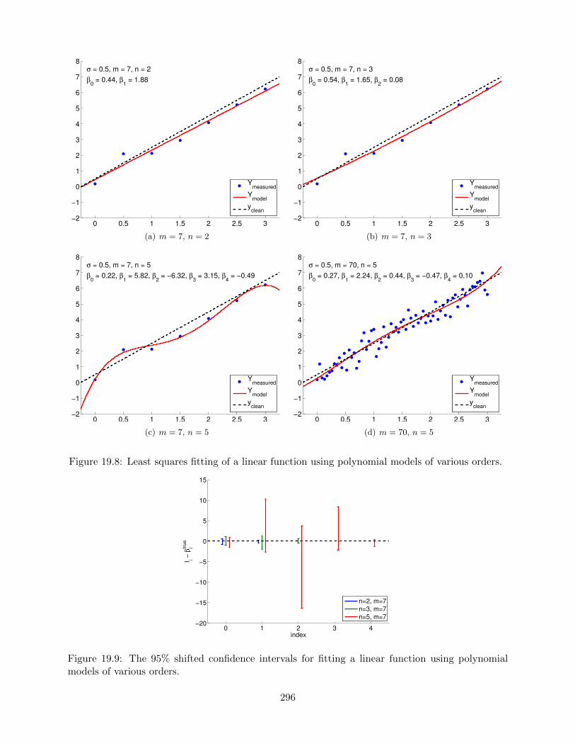
0 0.5 1 1.5 2 2.5 3−2

−1

0

1

2

3

4

5

6

7

8

σ = 0.5, m = 7, n = 2

β0 = 0.44, β

1 = 1.88

Ymeasured

Ymodel

yclean

(a) m = 7, n = 2

0 0.5 1 1.5 2 2.5 3−2

−1

0

1

2

3

4

5

6

7

8

σ = 0.5, m = 7, n = 3

β0 = 0.54, β

1 = 1.65, β

2 = 0.08

Ymeasured

Ymodel

yclean

(b) m = 7, n = 3

0 0.5 1 1.5 2 2.5 3−2

−1

0

1

2

3

4

5

6

7

8

σ = 0.5, m = 7, n = 5

β0 = 0.22, β

1 = 5.82, β

2 = −6.32, β

3 = 3.15, β

4 = −0.49

Ymeasured

Ymodel

yclean

(c) m = 7, n = 5

0 0.5 1 1.5 2 2.5 3−2

−1

0

1

2

3

4

5

6

7

8

σ = 0.5, m = 70, n = 5

β0 = 0.27, β

1 = 2.24, β

2 = 0.44, β

3 = −0.47, β

4 = 0.10

Ymeasured

Ymodel

yclean

(d) m = 70, n = 5

Figure 19.8: Least squares fitting of a linear function using polynomial models of various orders.

0 1 2 3 4−20

−15

−10

−5

0

5

10

15

index

I i − β

itru

e

n=2, m=7

n=3, m=7

n=5, m=7

Figure 19.9: The 95% shifted confidence intervals for fitting a linear function using polynomialmodels of various orders.

296

number of samples are required to tighten the confidence intervals — and improve our parameterestimates — for the overfitting cases. Thus, deducing an appropriate response model based on, forexample, physical principles can significantly improve the quality of the parameter estimates andthe performance of the predictive model.

·

Begin Advanced Material

Example 19.2.3 overfitting of a quadratic functionIn this example, we study the effect of overfitting in more detail. We consider data governed by arandom quadratic function of the form

Y (x) ∼ −1

2+

2

3x− 1

8cx2 +N (0, σ2) ,

with c = 1. We again consider for our model the polynomial form Ymodel,n(x;β).Figure 19.10(a) shows a typical result of fitting the data using m = 14 sampling points and

n = 4. Our cubic model includes the underlying quadratic distribution. Thus there is no bias andour noise assumptions are satisfied. However, compared to the quadratic model (n = 3), the cubicmodel is affected by the noise in the measurement and produces spurious variations. This spuriousvariation tend to disappear with the number of sampling points, and Figure 19.10(b) with m = 140sampling points exhibits a more stable fit.

Figure 19.10(c) shows a realization of confidence intervals for the cubic model (n = 4) usingm = 14 and m = 140 sampling points. A realization of confidence intervals for the quadratic model(n = 3) is also shown for comparison. Using the same set of data, the confidence intervals for thecubic model are larger than those of the quadratic model. However, the confidence intervals of thecubic model include the true parameter value for most cases. Figure 19.10(d) confirms that the95% of the realization of the confidence intervals include the true parameter. Thus, the confidenceintervals are reliable indicators of the quality of the parameter estimates, and in general the intervalsget tighter with m, as expected. Modest overfitting, n = 4 vs. n = 3, with m sufficiently large,poses little threat.

Let us check how overfitting affects the quality of the fit using two different measures. The firstis a measure of how well we can predict, or reproduce, the clean underlying function; the second isa measure for how well we approximate the underlying parameters.

First, we quantify the quality of prediction using the maximum difference in the model and theclean underlying data,

emax ≡ maxx∈[−1/4,3+1/4]

|Ymodel,n(x; β)− Yclean(x)| .

Figure 19.11(a) shows the variation in the maximum prediction error with n for a few differentvalues of m. We see that we get the closest fit (in the sense of the maximum error), when n = 3— when there are no “extra” terms in our model. When only m = 7 data points are used, thequality of the regression degrades significantly as we overfit the data (n > 3). As the dimension ofthe model n approaches the number of measurements, m, we are effectively interpolating the noise.The interpolation induces a large error in the parameter estimates, and we can not estimate thenoise since we are fitting the noise. We observe in general that the quality of the estimate improvesas the number of samples is increased.

Second, we quantify the quality of the parameter estimates by measuring the error in thequadratic coefficient, i.e., |β2 − β2|. Figure 19.11(b) shows that, not surprisingly, the error in the

297

0 0.5 1 1.5 2 2.5 3−0.8

−0.6

−0.4

−0.2

0

0.2

0.4

0.6

Ymeasured

Ymodel

yclean

(a) m = 14

0 0.5 1 1.5 2 2.5 3−0.8

−0.6

−0.4

−0.2

0

0.2

0.4

0.6

Ymeasured

Ymodel

yclean

(b) m = 140

0 1 2 3−0.8

−0.6

−0.4

−0.2

0

0.2

0.4

0.6

index

I i − β

itrue

n=4, m=14

n=4, m=140

n=3, m=14

n=3, m=140

(c) 95% shifted confidence intervals

0 1 2 30

0.1

0.2

0.3

0.4

0.5

0.6

0.7

0.8

0.9

1

fraction in

index

95% confidence

(d) 95% ci in/out (100 realizations, m = 140)

Figure 19.10: Least squares fitting of a quadratic function (c = 1) using a cubic model.

298

1 2 3 4 5 60

0.1

0.2

0.3

0.4

0.5

0.6

0.7

0.8

n

ma

xim

um

err

or

m=7

m=14

m=140

(a) maximum prediction error

1 2 3 4 5 610

−3

10−2

10−1

100

101

n

β2 e

rro

r

m=7

m=14

m=140

(b) error in parameter β2

1 2 3 4 5 610−3

10−2

10−1

100

n

||Y−

X β

||/m

1/2

m=7m=14m=140

^

(c) (normalized) residual

1 2 3 4 5 610

0

101

102

103

104

105

n

νm

ax/ν

min

m=7

m=14

m=140

(d) condition number

Figure 19.11: Variation in the quality of regression with overfitting.

299

parameter increases under overfitting. In particular, for the small sample size of m = 7, the errorin the estimate for β3 increases from O(10−2) for n = 3 to O(1) for n ≥ 5. Since β3 is an O(1)quantity, this renders the parameter estimates for n ≥ 5 essentially meaningless.

It is important to recognize that the degradation in the quality of estimate — either in termsof predictability or parameter error — is not due to the poor fit at the data points. In particular,the (normalized) residual,

1

m1/2‖Y −Xβ‖ ,

which measures the fit at the data points, decreases as n increases, as shown in Figure 19.11(c). Thedecrease in the residual is not surprising. We have new coefficients which were previously implicitlyzero and hence the least squares must provide a residual which is non-increasing as we increasen and let these coefficients realize their optimal values (with respect to residual minimization).However, as we see in Figure 19.11(a) and 19.11(b), better fit at data points does not imply betterrepresentation of the underlying function or parameters.

The worse prediction of the parameter is due to the increase in the conditioning of the problem(νmax/νmin), as shown in Figure 19.11(d). Recall that the error in the parameter is a function ofboth residual (goodness of fit at data points) and conditioning of the problem, i.e.

‖β − β‖‖β‖ ≤ νmax

νmin

‖Xβ − Y ‖‖Y ‖ .

As we increase n for a fixed m, we do reduce the residual. However, clearly the error is larger bothin terms of output prediction and parameter estimate. Once again we see that the residual — andsimilar commonly used goodness of fit statistics such as R2 — is not the “final answer” in terms ofthe success of any particular regression exercise.

Fortunately, similar to the previous example, this poor estimate of the parameters is reflectedin large confidence intervals, as shown in Figure 19.12. Thus, while the estimates may be poor, weare informed that we should not have much confidence in our estimate of the parameters and thatwe need more data points to improve the fit.

Finally, we note that the conditioning of the problem reflects where we choose to make ourmeasurements, our choice of response model, and how we choose to represent this response model.For example, as regards the latter, a Legendre (polynomial) expansion of order n would certainlydecrease νmax/νmin, albeit at some complication in how we extract various parameters of interest.

·

Example 19.2.4 underfitting of a quadratic functionWe consider data governed by a noisy quadratic function (ntrue ≡ 3) of the form

Y (x) ∼ −1

2+

2

3x− 1

8cx2 +N (0, σ2) .

We again assume that the input-output dependency is unknown. The focus of this example isunderfitting; i.e., the case in which the degree of freedom of the model n is less than that of datantrue. In particular, we will consider an affine model (n = 2),

Ymodel,2(x;β) = β0 + β1x ,

which is clearly biased (unless c = 0).For the first case, we consider the true underlying distribution with c = 1, which results in a

strong quadratic dependency of Y on x. The result of fitting the function is shown in Figure 19.13.

300

0 1 2 3 4 5−4

−3

−2

−1

0

1

2

3

4

5

index

I i − β

itru

e

n=3, m=14

n=4, m=14

n=5, m=14

n=6, m=14

(a) m = 14

0 1 2 3 4 5−2.5

−2

−1.5

−1

−0.5

0

0.5

1

1.5

2

index

I i − β

itrue

n=3, m=140

n=4, m=140

n=5, m=140

n=6, m=140

(b) m = 140

Figure 19.12: The variation in the confidence intervals for fitting a quadratic function usingquadratic (n = 3), cubic (n = 4), quartic (n = 5), and quintic (n = 6) polynomials. Note thedifference in the scales for the m = 14 and m = 140 cases.

Note that the affine model is incapable of representing the quadratic dependency even in the absenceof noise. Thus, comparing Figure 19.13(a) and 19.13(b), the fit does not improve with the numberof sampling points.

Figure 19.13(c) shows typical individual confidence intervals for the affine model (n = 2) usingm = 14 and m = 140 sampling points. Typical confidence intervals for the quadratic model (n = 3)are also provided for comparison. Let us first focus on analyzing the fit of the affine model (n = 2)using m = 14 sampling points. We observe that this realization of confidence intervals I0 and I1

does not include the true parameters βtrue0 and βtrue

1 , respectively. In fact, Figure 19.13(d) showsthat only 37 of the 100 realizations of the confidence interval I0 include βtrue

0 and that none of therealizations of I1 include βtrue

1 . Thus the frequency that the true value lies in the confidence intervalis significantly lower than 95%. This is due to the presence of the bias error, which violates ourassumptions about the behavior of the noise — the assumptions on which our confidence intervalestimate rely. In fact, as we increase the number of sampling point from m = 14 to m = 140 wesee that the confidence intervals for both β0 and β1 tighten; however, they converge toward wrongvalues. Thus, in the presence of bias, the confidence intervals are unreliable, and their convergenceimplies little about the quality of the estimates.

Let us now consider the second case with c = 1/10. This case results in a much weakerquadratic dependency of Y on x. Typical fits obtained using the affine model are shown in Fig-ure 19.14(a) and 19.14(b) for m = 14 and m = 140 sampling points, respectively. Note that the fitis better than the c = 1 case because the c = 1/10 data can be better represented using the affinemodel.

Typical confidence intervals, shown in Figure 19.14(c), confirm that the confidence intervals aremore reliable than in the c = 1 case. Of the 100 realizations for the m = 14 case, 87% and 67%of the confidence intervals include the true values βtrue

0 and βtrue1 , respectively. The frequencies

are lower than the 95%, i.e., the confidence intervals are not as reliable as their pretension, dueto the presence of bias. However, they are more reliable than the case with a stronger quadraticdependence, i.e. a stronger bias. Recall that a smaller bias leading to a smaller error is consistentwith the deterministic error bounds we developed in the presence of bias.

Similar to the c = 1 case, the confidence interval tightens with the number of samples m, but

301

0 0.5 1 1.5 2 2.5 3−0.8

−0.6

−0.4

−0.2

0

0.2

0.4

0.6

Ymeasured

Ymodel

yclean

(a) m = 14

0 0.5 1 1.5 2 2.5 3−0.8

−0.6

−0.4

−0.2

0

0.2

0.4

0.6

Ymeasured

Ymodel

yclean

(b) m = 140

0 1 2−0.5

−0.4

−0.3

−0.2

−0.1

0

0.1

0.2

0.3

index

I i − β

itrue

n=2, m=14

n=2, m=140

n=3, m=14

n=3, m=140

(c) 95% shifted confidence intervals

0 10

0.1

0.2

0.3

0.4

0.5

0.6

0.7

0.8

0.9

1

fraction in

index

95% confidence

(d) 95% ci in/out (100 realizations, m = 14)

Figure 19.13: Least squares fitting of a quadratic function (c = 1) using an affine model.

302

0 0.5 1 1.5 2 2.5 3−1

−0.5

0

0.5

1

1.5

2

Ymeasured

Ymodel

yclean

(a) m = 14

0 0.5 1 1.5 2 2.5 3−1

−0.5

0

0.5

1

1.5

2

Ymeasured

Ymodel

yclean

(b) m = 140

0 1 2−0.25

−0.2

−0.15

−0.1

−0.05

0

0.05

0.1

0.15

0.2

index

I i − β

itrue

n=2, m=14

n=2, m=140

n=3, m=14

n=3, m=140

(c) 95% shifted confidence intervals

0 10

0.1

0.2

0.3

0.4

0.5

0.6

0.7

0.8

0.9

1

fraction in

index

95% confidence

(d) 95% ci in/out (100 realizations, m = 14)

Figure 19.14: Least squares fitting of a quadratic function (c = 1/10) using an affine model.

303

they converge to a wrong value. Accordingly, the reliability of the confidence intervals decreaseswith m.

·

End Advanced Material

304

Unit IV

(Numerical) Differential Equations

305

Chapter 20

Motivation

Although mobile robots operating in flat, indoor environments can often perform quite wellwithout any suspension, in uneven terrain, a well-designed suspension can be critical.

An actual robot suspension and its simplified model are shown in Figure 20.1. The rear and frontsprings with spring constants k1 and k2 serve to decouple the rest of the robot chassis from thewheels, allowing the chassis and any attached instrumentation to “float” relatively unperturbedwhile the wheels remain free to follow the terrain and maintain traction. The rear and frontdampers with damping coefficients c1 and c2 (shown here inside the springs) dissipate energy toprevent excessive chassis displacements (e.g., from excitation of a resonant mode) and oscillations.Note that in our “half-robot” model, k1 accounts for the combined stiffness of both rear wheels,and k2 accounts for the combined stiffness of both front wheels. Similarly, c1 and c2 account forthe combined damping coefficients of both rear wheels and both front wheels, respectively.

We are particularly concerned with the possibility of either the front or rear wheels losing contactwith the ground, the consequences of which — loss of control and a potentially harsh landing —we wish to avoid.

To aid in our understanding of robot suspensions and, in particular, to understand the condi-tions resulting in loss of contact, we wish to develop a simulation based on the simple model ofFigure 20.1(b). Specifically, we wish to simulate the transient (time) response of the robot withsuspension traveling at some constant velocity v over a surface with profile H(x), the height of theground as a function of x, and to check if loss of contact occurs. To do so, we must integrate thedifferential equations of motion for the system.

First, we determine the motion at the rear (subscript 1) and front (subscript 2) wheels in orderto calculate the normal forces N1 and N2. Because we assume constant velocity v, we can determinethe position in x of the center of mass at any time t (we assume X(t = 0) = 0) as

X = vt . (20.1)

Given the current state Y , Y , θ (the inclination of the chassis), and θ, we can then calculate the

307

DRAFT V2.1 © The Authors. License: Creative Commons BY-NC-SA 3.0.

(a) Actual robot suspension.

H(x)

θ

mg

N1

N2

Y

v

x

y

h2

m,Izz

L2L1

k ,c1 1 k ,c2 2

(b) Robot suspension model.

Figure 20.1: Mobile robot suspension

positions and velocities in both x and y at the rear and front wheels (assuming θ is small) as

X1 = X − L1, (X1 = v) ,

X2 = X + L2, (X2 = v) ,

Y1 = Y − L1θ ,

Y1 = Y − L1θ ,

Y2 = Y + L2θ ,

Y2 = Y + L2θ ,

(20.2)

where L1 and L2 are the distances to the system’s center of mass from the rear and front wheels.(Recall ˙ refers to time derivative.) Note that we define Y = 0 as the height of the robot’s centerof mass with both wheels in contact with flat ground and both springs at their unstretched anduncompressed lengths, i.e., when N1 = N2 = 0. Next, we determine the heights of the ground atthe rear and front contact points as

h1 = H(X1) ,

h2 = H(X2) .(20.3)

Similarly, the rates of change of the ground height at the rear and front are given by

dh1

dt= h1 = v

d

dxH(X1) ,

dh2

dt= h2 = v

d

dxH(X2) .

(20.4)

Note that we must multiply the spatial derivatives dHdx by v = dX

dt to find the temporal derivatives.While the wheels are in contact with the ground we can determine the normal forces at the rear

and front from the constitutive equations for the springs and dampers as

N1 = k1(h1 − Y1) + c1(h1 − Y1) ,

N2 = k2(h2 − Y2) + c2(h2 − Y2) .(20.5)

308

If either N1 or N2 is calculated from Equations (20.5) to be less than or equal to zero, we candetermine that the respective wheel has lost contact with the ground and stop the simulation,concluding loss of contact, i.e., failure.

Finally, we can determine the rates of change of the state from the linearized (cos θ ≈ 1,sin θ ≈ θ) equations of motion for the robot, given by Newton-Euler as

X = 0, X = v, X(0) = 0 ,

Y = −g +N1 +N2

m, Y (0) = Y0, Y (0) = Y0 ,

θ =N2L2 −N1L1

Izz, θ(0) = θ0, θ(0) = θ0 ,

(20.6)

where m is the mass of the robot, and Izz is the moment of inertia of the robot about an axisparallel to the Z axis passing through the robot’s center of mass.

In this unit we shall discuss the numerical procedures by which to integrate systems of ordinarydifferential equations such as (20.6). This integration can then permit us to determine loss ofcontact and hence failure.

309

310

Chapter 21

Initial Value Problems

21.1 Scalar First-Order Linear ODEs

21.1.1 Model Problem

Let us consider a canonical initial value problem (IVP),

du

dt= λu+ f(t), 0 < t < tf ,

u(0) = u0 .

The objective is to find u over all time t ∈ ]0, tf ] that satisfies the ordinary differential equation(ODE) and the initial condition. This problem belongs to the class of initial value problems (IVP)since we supplement the equation with condition(s) only at the initial time. The ODE is first orderbecause the highest derivative that appears in the equation is the first-order derivative; because itis first order, only one initial condition is required to define a unique solution. The ODE is linearbecause the expression is linear with respect to u and its derivative du/dt; note that f does not haveto be a linear function of t for the ODE to be linear. Finally, the equation is scalar since we haveonly a single unknown, u(t) ∈ R. The coefficient λ ∈ R controls the behavior of the ODE; λ < 0results in a stable (i.e. decaying) behavior, whereas λ > 0 results in an unstable (i.e. growing)behavior.

We can motivate this model problem (with λ < 0) physically with a simple heat transfersituation. We consider a body at initial temperature u0 > 0 which is then “dunked” or “immersed”into a fluid flow — forced or natural convection — of ambient temperature (away from the body)zero. (More physically, we may view u0 as the temperature elevation above some non-zero ambienttemperature.) We model the heat transfer from the body to the fluid by a heat transfer coefficient,h. We also permit heat generation within the body, q(t), due (say) to Joule heating or radiation.If we now assume that the Biot number — the product of h and the body “diameter” in thenumerator, thermal conductivity of the body in the denominator — is small, the temperature ofthe body will be roughly uniform in space. In this case, the temperature of the body as a functionof time, u(t), will be governed by our ordinary differential equation (ODE) initial value problem(IVP), with λ = −hArea/ρcVol and f(t) = q(t)/ρcVol, where ρ and c are the body density andspecific heat, respectively, and Area and Vol are the body surface area and volume, respectively.

311

DRAFT V2.1 © The Authors. License: Creative Commons BY-NC-SA 3.0.

In fact, it is possible to express the solution to our model problem in closed form (as a con-volution). Our interest in the model problem is thus not because we require a numerical solutionprocedure for this particular simple problem. Rather, as we shall see, our model problem willprovide a foundation on which to construct and understand numerical procedures for much moredifficult problems — which do not admit closed-form solution.

21.1.2 Analytical Solution

Before we pursue numerical methods for solving the IVP, let us study the analytical solution fora few cases which provide insight into the solution and also suggest test cases for our numericalapproaches.

Homogeneous Equation

The first case considered is the homogeneous case, i.e., f(t) = 0. Without loss of generality, let usset u0 = 1. Thus, we consider

du

dt= λu, 0 < t < tf ,

u(0) = 1 .

We find the analytical solution by following the standard procedure for obtaining the homogeneoussolution, i.e., substitute u = αeβt to obtain

(LHS) =du

dt=

d

dt(αeβt) = αβet ,

(RHS) = λαeβt .

Equating the LHS and RHS, we obtain β = λ. The solution is of the form u(t) = αeλt. Thecoefficient α is specified by the initial condition, i.e.

u(t = 0) = α = 1 ;

thus, the coefficient is α = 1. The solution to the homogeneous ODE is

u(t) = eλt .

Note that solution starts from 1 (per the initial condition) and decays to zero for λ < 0. The decayrate is controlled by the time constant 1/|λ| — the larger the λ, the faster the decay. The solutionfor a few different values of λ are shown in Figure 21.1.

We note that for λ > 0 the solution grows exponentially in time: the system is unstable. (Inactual fact, in most physical situations, at some point additional terms — for example, nonlineareffects not included in our simple model — would become important and ensure saturation insome steady state.) In the remainder of this chapter unless specifically indicated otherwise we shallassume that λ < 0.

Constant Forcing

Next, we consider a constant forcing case with u0 = 0 and f(t) = 1, i.e.

du

dt= λu+ 1 ,

u0 = 0 .

312

0 1 2 3 4 50

0.1

0.2

0.3

0.4

0.5

0.6

0.7

0.8

0.9

1

t

u(t

)

λ = −1

λ = −0.5

λ = −4.0

Figure 21.1: Solutions to the homogeneous equation.

We have already found the homogeneous solution to the ODE. We now find the particular solution.Because the forcing term is constant, we consider a particular solution of the form up(t) = γ.Substitution of up yields

0 = λγ + 1 ⇒ γ = − 1

λ.

Thus, our solution is of the form

u(t) = − 1

λ+ αeλt .

Enforcing the initial condition,

u(t = 0) = − 1

λ+ α = 0 ⇒ α =

1

λ.

Thus, our solution is given by

u(t) =1

λ

(eλt − 1

).

The solutions for a few different values of λ are shown in Figure 21.2. For λ < 0, after the transientwhich decays on the time scale 1/|λ|, the solution settles to the steady state value of −1/λ.

Sinusoidal Forcing

Let us consider a final case with u0 = 0 and a sinusoidal forcing, f(t) = cos(ωt), i.e.

du

dt= λu+ cos(ωt) ,

u0 = 0 .

Because the forcing term is sinusoidal with the frequency ω, the particular solution is of the formup(t) = γ sin(ωt) + δ cos(ωt). Substitution of the particular solution to the ODE yields

(LHS) =dupdt

= ω(γ cos(ωt)− δ sin(ωt)) ,

(RHS) = λ(γ sin(ωt) + δ cos(ωt)) + cos(ωt) .

313

0 1 2 3 4 50

0.2

0.4

0.6

0.8

1

1.2

1.4

1.6

1.8

2

t

u(t

)

λ = −1

λ = −0.5

λ = −4.0

Figure 21.2: Solutions to the ODE with unit constant forcing.

Equating the LHS and RHS and collecting like coefficients we obtain

ωγ = λδ + 1 ,

−ωδ = λγ .

The solution to this linear system is given by γ = ω/(ω2 + λ2) and δ = −λ/(ω2 + λ2). Thus, thesolution is of the form

u(t) =ω

ω2 + λ2sin(ωt)− λ

ω2 + λ2cos(ωt) + αeλt .

Imposing the boundary condition, we obtain

u(t = 0) = − λ

ω2 + λ2+ α = 0 ⇒ α =

λ

ω2 + λ2.

Thus, the solution to the IVP with the sinusoidal forcing is

u(t) =ω

ω2 + λ2sin(ωt)− λ

ω2 + λ2

(cos(ωt)− eλt

).

We note that for low frequency there is no phase shift; however, for high frequency there is a π/2phase shift.

The solutions for λ = −1, ω = 1 and λ = −20, ω = 1 are shown in Figure 21.3. The steadystate behavior is controlled by the sinusoidal forcing function and has the time scale of 1/ω. Onthe other hand, the initial transient is controlled by λ and has the time scale of 1/|λ|. In particular,note that for |λ| � ω, the solution exhibits very different time scales in the transient and in thesteady (periodic) state. This is an example of a stiff equation (we shall see another example at theconclusion of this unit). Solving a stiff equation introduces additional computational challenges fornumerical schemes, as we will see shortly.

21.1.3 A First Numerical Method: Euler Backward (Implicit)

In this section, we consider the Euler Backward integrator for solving initial value problems. Wefirst introduce the time stepping scheme and then discuss a number of properties that characterizethe scheme.

314

0 1 2 3 4 5−1

0

1

t

u(t

)

0 1 2 3 4 5−0.05

0

0.05

λ = −1, ω = −1

λ = −20, ω = −1

Figure 21.3: Solutions to the ODE with sinusoidal forcing.

Discretization

In order to solve an IVP numerically, we first discretize the time domain ]0, tf ] into J segments.The discrete time points are given by

tj = j∆t, j = 0, 1, . . . , J = tf/∆t ,

where ∆t is the time step. For simplicity, we assume in this chapter that the time step is constantthroughout the time integration.

The Euler Backward method is obtained by applying the first-order Backward Difference For-mula (see Unit I) to the time derivative. Namely, we approximate the time derivative by

du

dt≈ uj − uj−1

∆t,

where uj = u(tj) is the approximation to u(tj) and ∆t = tj − tj−1 is the time step. Substitutingthe approximation into the differential equation, we obtain a difference equation

uj − uj−1

∆t= λuj + f(tj), j = 1, . . . , J ,

u0 = u0 ,

for uj , j = 0, . . . , J . Note the scheme is called “implicit” because time level j appears on theright-hand side. We can think of Euler Backward as a kind of rectangle, right integration rule —but now the integrand is not known a priori .

We anticipate that the solution uj , j = 1, . . . , J , approaches the true solution u(tj), j = 1, . . . , J ,as the time step gets smaller and the finite difference approximation approaches the continuous sys-tem. In order for this convergence to the true solution to take place, the discretization must possesstwo important properties: consistency and stability. Note our analysis here is more subtle thanthe analysis in Unit I. In Unit I we looked at the error in the finite difference approximation; here,we are interested in the error induced by the finite difference approximation on the approximatesolution of the ODE IVP.

315

Consistency

Consistency is a property of a discretization that ensures that the discrete equation approximatesthe same process as the underlying ODE as the time step goes to zero. This is an importantproperty, because if the scheme is not consistent with the ODE, then the scheme is modeling adifferent process and the solution would not converge to the true solution.

Let us define the notion of consistency more formally. We first define the truncation error bysubstituting the true solution u(t) into the Euler Backward discretization, i.e.

τ jtrunc ≡u(tj)− u(tj−1)

∆t− λu(tj)− f(tj), j = 1, . . . , J .

Note that the truncation error, τ jtrunc, measures the extent to which the exact solution to the ODEdoes not satisfy the difference equation. In general, the exact solution does not satisfy the differenceequation, so τ jtrunc 6= 0. In fact, as we will see shortly, if τ jtrunc = 0, j = 1, . . . , J , then uj = u(tj),i.e., uj is the exact solution to the ODE at the time points.

We are particularly interested in the largest of the truncation errors, which is in a sense thelargest discrepancy between the differential equation and the difference equation. We denote thisusing the infinity norm,

‖τtrunc‖∞ = maxj=1,...,J

|τ jtrunc| .

A scheme is consistent with the ODE if

‖τtrunc‖∞ → 0 as ∆t→ 0 .

The difference equation for a consistent scheme approaches the differential equation as ∆t →0. However, this does not necessary imply that the solution to the difference equation, u(tj),approaches the solution to the differential equation, u(tj).

The Euler Backward scheme is consistent. In particular

‖τtrunc‖∞ ≤∆t

2maxt∈[0,tf ]

∣∣∣∣∣d2u

dt2(t)

∣∣∣∣∣→ 0 as ∆t→ 0 .

We demonstrate this result below.

Begin Advanced Material

Let us now analyze the consistency of the Euler Backward integration scheme. We first applyTaylor expansion to u(tj−1) about tj , i.e.

u(tj−1) = u(tj)−∆tdu

dt(tj)−

∫ tj

tj−1

(∫ τ

tj−1

d2u

dt2(γ)dγ

)dτ︸ ︷︷ ︸

sj(u)

.

This result is simple to derive. By the fundamental theorem of calculus,∫ τ

tj−1

du2

dt2(γ)dγ =

du

dt(τ)− du

dt(tj−1) .

316

Integrating both sides over ]tj−1, tj [,∫ tj

tj−1

(∫ τ

tj−1

du2

dt2(γ)dγ

)dτ =

∫ tj

tj−1

(du

dt(τ)

)dτ −

∫ tj

tj−1

(du

dt(tj−1)

)dτ

= u(tj)− u(tj−1)− (tj − tj−1)du

dt(tj−1)

= u(tj)− u(tj−1)−∆tdu

dt(tj−1) .

Substitution of the expression to the right-hand side of the Taylor series expansion yields

u(tj)−∆tdu

dt(tj)− sj(u) = u(tj)−∆t

du

dt(tj)− u(tj) + u(tj−1) + ∆t

du

dt(tj−1) = u(tj−1) ,

which proves the desired result.Substituting the Taylor expansion into the expression for the truncation error,

τ jtrunc =u(tj)− u(tj−1)

∆t− λu(tj)− f(tj)

=1

∆t

(u(tj)−

(u(tj)−∆t

du

dt(tj)− sj(u)

))− λu(tj)− f(tj)

=du

dt(tj)− λu(tj)− f(tj)︸ ︷︷ ︸

=0 : by ODE

+sj(u)

∆t

=sj(u)

∆t.

We now bound the remainder term sj(u) as a function of ∆t. Note that

sj(u) =

∫ tj

tj−1

(∫ τ

tj−1

d2u

dt2(γ)dγ

)dτ ≤

∫ tj

tj−1

(∫ τ

tj−1

∣∣∣∣∣d2u

dt2(γ)

∣∣∣∣∣ dγ)dτ

≤ maxt∈[tj−1,tj ]

∣∣∣∣∣d2u

dt2(t)

∣∣∣∣∣∫ tj

tj−1

∫ τ

tj−1

dγdτ

= maxt∈[tj−1,tj ]

∣∣∣∣∣d2u

dt2(t)

∣∣∣∣∣ ∆t2

2, j = 1, . . . , J .

So, the maximum truncation error is

‖τtrunc‖∞ = maxj=1,...,J

|τ jtrunc| ≤ maxj=1,...,J

(1

∆tmax

t∈[tj−1,tj ]

∣∣∣∣∣d2u

dt2(t)

∣∣∣∣∣ ∆t2

2

)≤ ∆t

2maxt∈[0,tf ]

∣∣∣∣∣d2u

dt2(t)

∣∣∣∣∣ .We see that

‖τtrunc‖∞ ≤∆t

2maxt∈[0,tf ]

∣∣∣∣∣d2u

dt2(t)

∣∣∣∣∣→ 0 as ∆t→ 0 .

Thus, the Euler Backward scheme is consistent.

End Advanced Material

317

Stability

Stability is a property of a discretization that ensures that the error in the numerical approximationdoes not grow with time. This is an important property, because it ensures that a small truncationerror introduced at each time step does not cause a catastrophic divergence in the solution overtime.

To study stability, let us consider a homogeneous IVP,

du

dt= λu ,

u(0) = 1 .

Recall that the true solution is of the form u(t) = eλt and decays for λ < 0. Applying the EulerBackward scheme, we obtain

uj − uj−1

∆t= λuj , j = 1, . . . , J ,

u0 = 1 .

A scheme is said to be absolutely stable if

|uj | ≤ |uj−1|, j = 1, . . . , J .

Alternatively, we can define the amplification factor, γ, as

γ ≡ |uj ||uj−1| .

Absolute stability requires that γ ≤ 1 for all j = 1, . . . , J .Let us now show that the Euler Backward scheme is stable for all ∆t (for λ < 0). Rearranging

the difference equation,

uj − uj−1 = λ∆t uj

uj(1− λ∆t) = uj−1

|uj | |1− λ∆t| = |uj−1| .

So, we have

γ =|uj ||uj−1| =

1

|1− λ∆t| .

Recalling that λ < 0 (and ∆t > 0), we have

γ =1

1− λ∆t< 1 .

Thus, the Euler Backward scheme is stable for all ∆t for the model problem considered. Thescheme is said to be unconditionally stable because it is stable for all ∆t. Some schemes are onlyconditionally stable, which means the scheme is stable for ∆t ≤ ∆tcr, where ∆tcr is some criticaltime step.

318

Convergence: Dahlquist Equivalence Theorem

Now we define the notion of convergence. A scheme is convergent if the numerical approximationapproaches the analytical solution as the time step is reduced. Formally, this means that

uj ≡ u(tj)→ u(tj) for fixed tj as ∆t→ 0 .

Note that fixed time tj means that the time index must go to infinity (i.e., an infinite number oftime steps are required) as ∆t → 0 because tj = j∆t. Thus, convergence requires that not toomuch error is accumulated at each time step. Furthermore, the error generated at a given stepshould not grow over time.

The relationship between consistency, stability, and convergence is summarized in the Dahlquistequivalence theorem. The theorem states that consistency and stability are the necessary andsufficient condition for a convergent scheme, i.e.

consistency + stability⇔ convergence .

Thus, we only need to show that a scheme is consistent and (absolutely) stable to show thatthe scheme is convergent. In particular, the Euler Backward scheme is convergent because it isconsistent and (absolutely) stable.

Begin Advanced Material

Example 21.1.1 Consistency, stability, and convergence for Euler BackwardIn this example, we will study in detail the relationship among consistency, stability, and conver-gence for the Euler Backward scheme. Let us denote the error in the solution by ej ,

ej ≡ u(tj)− u(tj) .

We first relate the evolution of the error to the truncation error. To begin, we recall that

u(tj)− u(tj−1)− λ∆tu(tj)−∆tf(tj) = ∆tτ jtrunc ,

u(tj)− u(tj−1)− λ∆tu(tj)−∆tf(tj) = 0 ;

subtracting these two equations and using the definition of the error we obtain

ej − ej−1 − λ∆tej = ∆tτ jtrunc ,

or, rearranging the equation,

(1− λ∆t)ej − ej−1 = ∆tτ jtrunc .

We see that the error itself satisfies the Euler Backward difference equation with the truncationerror as the source term. Clearly, if the truncation error τ jtrunc is zero for all time steps (and initialerror is zero), then the error remains zero. In other words, if the truncation error is zero then thescheme produces the exact solution at each time step.

However, in general, the truncation error is nonzero, and we would like to analyze its influenceon the error. Let us multiply the equation by (1− λ∆t)j−1 to get

(1− λ∆t)jej − (1− λ∆t)j−1ej−1 = (1− λ∆t)j−1∆tτ jtrunc ,

319

Now, let us compute the sum for j = 1, . . . , n, for some n ≤ J ,

n∑j=1

[(1− λ∆t)jej − (1− λ∆t)j−1ej−1

]=

n∑j=1

[(1− λ∆t)j−1∆tτ jtrunc

].

This is a telescopic series and all the middle terms on the left-hand side cancel. More explicitly,

(1− λ∆t)nen − (1− λ∆t)n−1en−1 = (1− λ∆t)n−1∆tτntrunc

(1− λ∆t)n−1en−1 − (1− λ∆t)n−2en−2 = (1− λ∆t)n−2∆tτn−1trunc

...

(1− λ∆t)2e2 − (1− λ∆t)1e1 = (1− λ∆t)1∆tτ2trunc

(1− λ∆t)1e1 − (1− λ∆t)0e0 = (1− λ∆t)0∆tτ1trunc

simplifies to

(1− λ∆t)nen − e0 =n∑j=1

(1− λ∆t)j−1∆tτ jtrunc .

Recall that we set u0 = u(t0) = u(t0), so the initial error is zero (e0 = 0). Thus, we are left with

(1− λ∆t)nen =

n∑j=1

(1− λ∆t)j−1∆tτ jtrunc

or, equivalently,

en =n∑j=1

(1− λ∆t)j−n−1∆tτ jtrunc .

Recalling that ‖τtrunc‖∞ = maxj=1,...,J |τ jtrunc|, we can bound the error by

|en| ≤ ∆t‖τtrunc‖∞n∑j=1

(1− λ∆t)j−n−1 .

Recalling the amplification factor for the Euler Backward scheme, γ = 1/(1−λ∆t), the summationcan be rewritten as

n∑j=1

(1− λ∆t)j−n−1 =1

(1− λ∆t)n+

1

(1− λ∆t)n−1+ · · ·+ 1

(1− λ∆t)

= γn + γn−1 + · · ·+ γ .

Because the scheme is stable, the amplification factor satisfies γ ≤ 1. Thus, the sum is bounded by

n∑j=1

(1− λ∆t)j−n−1 = γn + γn−1 + · · ·+ γ ≤ nγ ≤ n .

320

Thus, we have

|en| ≤ (n∆t)‖τtrunc‖∞ = tn‖τtrunc‖∞ .

Furthermore, because the scheme is consistent, ‖τtrunc‖∞ → 0 as ∆t→ 0. Thus,

‖en‖ ≤ tn‖τtrunc‖∞ → 0 as ∆t→ 0

for fixed tn = n∆t. Note that the proof of convergence relies on stability (γ ≤ 1) and consistency(‖τtrunc‖∞ → 0 as ∆t→ 0).

·

End Advanced Material

Order of Accuracy

The Dahlquist equivalence theorem shows that if a scheme is consistent and stable, then it isconvergent. However, the theorem does not state how quickly the scheme converges to the truesolution as the time step is reduced. Formally, a scheme is said to be pth-order accurate if

|ej | < C∆tp for a fixed tj = j∆t as ∆t→ 0 .

The Euler Backward scheme is first-order accurate (p = 1), because

‖ej‖ ≤ tj‖τtrunc‖∞ ≤ tj∆t

2maxt∈[0,tf ]

∣∣∣∣∣d2u

dt2(t)

∣∣∣∣∣ ≤ C∆t1

with

C =tf2

maxt∈[0,tf ]

∣∣∣∣∣d2u

dt2(t)

∣∣∣∣∣ .(We use here tj ≤ tf .)

In general, for a stable scheme, if the truncation error is pth-order accurate, then the scheme ispth-order accurate, i.e.

‖τtrunc‖∞ ≤ C∆tp ⇒ |ej | ≤ C∆tp for a fixed tj = j∆t .

In other words, once we prove the stability of a scheme, then we just need to analyze its truncationerror to understand its convergence rate. This requires little more work than checking for consis-tency. It is significantly simpler than deriving the expression for the evolution of the error andanalyzing the error behavior directly.

Figure 21.4 shows the error convergence behavior of the Euler Backward scheme applied to thehomogeneous ODE with λ = −4. The error is measured at t = 1. Consistent with the theory, thescheme converges at the rate of p = 1.

21.1.4 An Explicit Scheme: Euler Forward

Let us now introduce a new scheme, the Euler Forward scheme. The Euler Forward scheme isobtained by applying the first-order forward difference formula to the time derivative, i.e.

du

dt≈ uj+1 − uj

∆t.

321

0 0.2 0.4 0.6 0.8 10

0.1

0.2

0.3

0.4

0.5

0.6

0.7

0.8

0.9

1

t

u

∆t = 0.5

∆t = 0.125

∆t = 0.03125

exact

(a) solution

10−2

10−1

100

10−3

10−2

10−1

1.00

∆t

e(t

=1

)

(b) error

Figure 21.4: The error convergence behavior for the Euler Backward scheme applied to the homo-geneous ODE (λ = −4). Note e(t = 1) = |u(tj)− uj | at tj = j∆t = 1.

Substitution of the expression to the linear ODE yields a difference equation,

uj+1 − uj∆t

= λuj + f(tj), j = 0, . . . , J − 1 ,

u0 = u0 .

To maintain the same time index as the Euler Backward scheme (i.e., the difference equationinvolves the unknowns uj and uj−1), let us shift the indices to obtain

uj − uj−1

∆t= λuj−1 + f(tj−1), j = 1, . . . , J ,

u0 = u0 .

The key difference from the Euler Backward scheme is that the terms on the right-hand side areevaluated at tj−1 instead of at tj . Schemes for which the right-hand side does not involve timelevel j are known as “explicit” schemes. While the change may appear minor, this significantlymodifies the stability. (It also changes the computational complexity, as we will discuss later.) Wemay view Euler Forward as a kind of “rectangle, left” integration rule.

Let us now analyze the consistency and stability of the scheme. The proof of consistency issimilar to that for the Euler Backward scheme. The truncation error for the scheme is

τ jtrunc =u(tj)− u(tj−1)

∆t− λu(tj−1)− f(tj−1) .

To analyze the convergence of the truncation error, we apply Taylor expansion to u(tj) about tj−1

to obtain,

u(tj) = u(tj−1) + ∆tdu

dt(tj−1) +

∫ tj

tj−1

(∫ τ

tj−1

du2

dt2(γ)dγ

)dτ︸ ︷︷ ︸

sj(u)

.

322

Thus, the truncation error simplifies to

τ jtrunc =1

∆t

(u(tj−1) + ∆t

du

dt(tj−1) + sj(u)− u(tj−1)

)− λu(tj−1)− f(tj−1)

=du

dt(tj−1)− λu(tj−1)− f(tj−1)︸ ︷︷ ︸

=0 : by ODE

+sj(u)

∆t

=sj(u)

∆t.

In proving the consistency of the Euler Backward scheme, we have shown that sj(u) is bounded by

sj(u) ≤ maxt∈[tj−1,tj ]

∣∣∣∣∣d2u

dt2(t)

∣∣∣∣∣ ∆t2

2, j = 1, . . . , J .

Thus, the maximum truncation error is bounded by

‖τtrunc‖∞ ≤ maxt∈[0,tf ]

∣∣∣∣∣d2u

dt2(t)

∣∣∣∣∣ ∆t

2.

Again, the truncation error converges linearly with ∆t and the scheme is consistent because‖τtrunc‖∞ → 0 as ∆t → 0. Because the scheme is consistent, we only need to show that it isstable to ensure convergence.

To analyze the stability of the scheme, let us compute the amplification factor. Rearrangingthe difference equation for the homogeneous case,

uj − uj−1 = λ∆tuj−1

or|uj | = |1 + λ∆t||uj−1|

which givesγ = |1 + λ∆t| .

Thus, absolute stability (i.e., γ ≤ 1) requires

−1 ≤ 1 + λ∆t ≤ 1

−2 ≤ λ∆t ≤ 0 .

Noting λ∆t ≤ 0 is a trivial condition for λ < 0, the condition for stability is

∆t ≤ − 2

λ≡ ∆tcr .

Note that the Euler Forward scheme is stable only for ∆t ≤ 2/|λ|. Thus, the scheme is conditionallystable. Recalling the stability is a necessary condition for convergence, we conclude that the schemeconverges for ∆t ≤ ∆tcr, but diverges (i.e., blows up) with j if ∆t > ∆tcr.

Figure 21.5 shows the error convergence behavior of the Euler Forward scheme applied to thehomogeneous ODE with λ = −4. The error is measured at t = 1. The critical time step for stabilityis ∆tcr = −2/λ = 1/2. The error convergence plot shows that the error grows exponentially for

323

0 0.2 0.4 0.6 0.8 10

0.1

0.2

0.3

0.4

0.5

0.6

0.7

0.8

0.9

1

t

u

∆t = 0.125

∆t = 0.0625

∆t = 0.03125

exact

(a) solution

10−2

10−1

100

10−3

10−2

10−1

1.00

∆t

e(t

=1)

(b) error

Figure 21.5: The error convergence behavior for the Euler Forward scheme applied to du/dt = −4u.Note e(t = 1) = |u(tj)− uj | at tj = j∆t = 1.

∆t > 1/2. As ∆t tends to zero, the numerical approximation converges to the exact solution, andthe convergence rate (order) is p = 1 — consistent with the theory.

We should emphasize that the instability of the Euler Forward scheme for ∆t > ∆tcr is not due toround-off errors and floating point representation (which involves “truncation,” but not truncationof the variety discussed in this chapter). In particular, all of our arguments for instability hold ininfinite-precision arithmetic as well as finite-precision arithmetic. The instability derives from thedifference equation; the instability amplifies truncation error, which is a property of the differenceequation and differential equation. Of course, an unstable difference equation will also amplifyround-off errors, but that is an additional consideration and not the main reason for the explosionin Figure 21.5.

21.1.5 Stiff Equations: Implicit vs. Explicit

Stiff equations are the class of equations that exhibit a wide range of time scales. For example,recall the linear ODE with a sinusoidal forcing,

du

dt= λt+ cos(ωt) ,

with |λ| � ω. The transient response of the solution is dictated by the time constant 1/|λ|.However, this initial transient decays exponentially with time. The long time response is governedby the time constant 1/ω � 1/|λ|.

Let us consider the case with λ = −100 and ω = 4; the time scales differ by a factor of 25.The result of applying the Euler Backward and Euler Forward schemes with several different timesteps is shown in Figure 21.6. Recall that the Euler Backward scheme is stable for any time stepfor λ < 0. The numerical result confirms that the solution is bounded for all time steps considered.While a large time step (in particular ∆t > 1/|λ|) results in an approximation which does notcapture the initial transient, the long term behavior of the solution is still well represented. Thus,if the initial transient is not of interest, we can use a ∆t optimized to resolve only the long termbehavior associated with the characteristic time scale of 1/ω — in other words, ∆t ∼ O(1/10),

324

0 0.2 0.4 0.6 0.8 1

−0.01

−0.008

−0.006

−0.004

−0.002

0

0.002

0.004

0.006

0.008

0.01

t

u

∆t = 0.25

∆t = 0.0625

∆t = 0.015625

exact

(a) Euler Backward (solution)

10−3

10−2

10−1

100

10−6

10−5

10−4

10−3

1.00

∆t

e(t

=1

)

(b) Euler Backward (convergence)

0 0.2 0.4 0.6 0.8 1

−0.01

−0.008

−0.006

−0.004

−0.002

0

0.002

0.004

0.006

0.008

0.01

t

u

∆t = 0.25

∆t = 0.0625

∆t = 0.015625

exact

(c) Euler Forward (solution)

10−3

10−2

10−1

100

10−10

10−5

100

105

1010

1.00

∆t

e(t

=1

)

(d) Euler Forward (convergence)

Figure 21.6: Application of the Euler Backward and Euler Forward schemes to a stiff equation.Note e(t = 1) = |u(tj)− uj | at tj = j∆t = 1.

rather than ∆t ∼ O(1/|λ|). If |λ| � ω, then we significantly reduce the number of time steps (andthus the computational cost).

Unlike its implicit counterpart, the Euler Forward method is only conditionally stable. Inparticular, the critical time step for this problem is ∆tcr = 2/|λ| = 0.02. Thus, even if we are notinterested in the initial transient, we cannot use a large time step because the scheme would beunstable. Only one of the three numerical solution (∆t = 1/64 < ∆tcr) is shown in Figure 21.6(c)because the other two time steps (∆t = 1/16, ∆t = 1/4) result in an unstable discretization anda useless approximation. The exponential growth of the error for ∆t > ∆tcr is clearly reflected inFigure 21.6(d).

Stiff equations are ubiquitous in the science and engineering context; in fact, it is not uncommonto see scales that differ by over ten orders of magnitude. For example, the time scale associatedwith the dynamics of a passenger jet is several orders of magnitude larger than the time scaleassociated with turbulent eddies. If the dynamics of the smallest time scale is not of interest,then an unconditionally stable scheme that allows us to take arbitrarily large time steps may be

325

computationally advantageous. In particular, we can select the time step that is necessary to achievesufficient accuracy without any time step restriction arising from the stability consideration. Putanother way, integration of a stiff system using a conditionally stable method may place a stringentrequirement on the time step, rendering the integration prohibitively expensive. As none of theexplicit schemes are unconditionally stable, implicit schemes are often preferred for stiff equations.

We might conclude from the above that explicit schemes serve very little purpose. In fact, thisis not the case, because the story is a bit more complicated. In particular, we note that for EulerBackward, at every time step, we must effect a division operation, 1/(1− (λ∆t)), whereas for EulerForward we must effect a multiplication, 1 + (λ∆t). When we consider real problems of interest —systems, often large systems, of many and often nonlinear ODEs — these scalar algebraic operationsof division for implicit schemes and multiplication for explicit schemes will translate into matrixinversion (more precisely, solution of matrix equations) and matrix multiplication, respectively.In general, and as we shall see in Unit V, matrix inversion is much more costly than matrixmultiplication.

Hence the total cost equation is more nuanced. An implicit scheme will typically enjoy a largertime step and hence fewer time steps — but require more work for each time step (matrix solution).In contrast, an explicit scheme may require a much smaller time step and hence many more timesteps — but will entail much less work for each time step. For stiff equations in which the ∆t foraccuracy is much, much larger than the ∆tcr required for stability (of explicit schemes), typicallyimplicit wins. On the other hand, for non-stiff equations, in which the ∆t for accuracy might be onthe same order as ∆tcr required for stability (of explicit schemes), explicit can often win: in suchcases we would in any event (for reasons of accuracy) choose a ∆t ≈ ∆tcr; hence, since an explicitscheme will be stable for this ∆t, we might as well choose an explicit scheme to minimize the workper time step.

Begin Advanced Material

21.1.6 Unstable Equations

End Advanced Material

21.1.7 Absolute Stability and Stability Diagrams

We have learned that different integration schemes exhibit different stability characteristics. Inparticular, implicit methods tend to be more stable than explicit methods. To characterize thestability of different numerical integrators, let us introduce absolute stability diagrams. Thesediagrams allow us to quickly analyze whether an integration scheme will be stable for a givensystem.

Euler Backward

Let us construct the stability diagram for the Euler Backward scheme. We start with the homoge-neous equation

dz

dt= λz .

So far, we have only considered a real λ; now we allow λ to be a general complex number. (Laterλ will represent an eigenvalue of a system, which in general will be a complex number.) The Euler

326

Re(λ∆t)

Im(λ

∆t)

−3 −2 −1 0 1 2 3−3

−2

−1

0

1

2

3

Figure 21.7: The absolute stability diagram for the Euler Backward scheme.

Backward discretization of the equation is

zj − zj−1

∆t= λzj ⇒ zj = (1− (λ∆t))−1zj−1 .

Recall that we defined the absolute stability as the region in which the amplification factor γ ≡|zj |/|zj−1| is less than or equal to unity. This requires

γ =|zj ||zj−1| =

∣∣∣∣ 1

1− (λ∆t)

∣∣∣∣ ≤ 1 .

We wish to find the values of (λ∆t) for which the numerical solution exhibits a stable behavior(i.e., γ ≤ 1). A simple approach to achieve this is to solve for the stability boundary by setting theamplification factor to 1 = |eiθ|, i.e.

eiθ =1

1− (λ∆t).

Solving for (λ∆t), we obtain

(λ∆t) = 1− e−iθ .

Thus, the stability boundary for the Euler Backward scheme is a circle of unit radius (the “one”multiplying eiθ) centered at 1 (the one directly after the = sign).

To deduce on which side of the boundary the scheme is stable, we can check the amplificationfactor evaluated at a point not on the circle. For example, if we pick λ∆t = −1, we observe thatγ = 1/2 ≤ 1. Thus, the scheme is stable outside of the unit circle. Figure 21.7 shows the stabilitydiagram for the Euler Backward scheme. The scheme is unstable in the shaded region; it is stablein the unshaded region; it is neutrally stable, |zj | = |zj−1|, on the unit circle. The unshaded region(γ < 1) and the boundary of the shaded and unshaded regions (γ = 1) represent the absolutestability region; the entire picture is denoted the absolute stability diagram.

To gain understanding of the stability diagram, let us consider the behavior of the Euler Back-ward scheme for a few select values of λ∆t. First, we consider a stable homogeneous equation, withλ = −1 < 0. We consider three different values of λ∆t, −0.5, −1.7, and −2.2. Figure 21.8(a) shows

327

Re(λ∆t)

Im(λ

∆t)

−3 −2 −1 0 1 2 3−3

−2

−1

0

1

2

3

λ∆t = −0.5

λ∆t = −1.7

λ∆t = −2.2

(a) λ∆t for λ = −1

0 5 10 15

0

0.2

0.4

0.6

0.8

1

t

u

λ∆t = −0.5

λ∆t = −1.7

λ∆t = −2.2

exact

(b) solution (λ = −1)

Re(λ∆t)

Im(λ

∆t)

−3 −2 −1 0 1 2 3−3

−2

−1

0

1

2

3

λ∆t = 0.5

λ∆t = 1.7

λ∆t = 2.2

(c) λ∆t for λ = 1

0 5 10 1510

−2

100

102

104

106

108

1010

t

u

λ∆t = 0.5

λ∆t = 1.7

λ∆t = 2.2

exact

(d) solution (λ = 1)

Figure 21.8: The behavior of the Euler Backward scheme for selected values of (λ∆t).

the three points on the stability diagram that correspond to these choices of λ∆t. All three pointslie in the unshaded region, which is a stable region. Figure 21.8(b) shows that all three numericalsolutions decay with time as expected. While the smaller ∆t results in a smaller error, all schemesare stable and converge to the same steady state solution.

Begin Advanced Material

Next, we consider an unstable homogeneous equation, with λ = 1 > 0. We again considerthree different values of λ∆t, 0.5, 1.7, and 2.2. Figure 21.8(c) shows that two of these points liein the unstable region, while λ∆t = 2.2 lies in the stable region. Figure 21.8(d) confirms that thesolutions for λ∆t = 0.5 and 1.7 grow with time, while λ∆t = 2.2 results in a decaying solution.The true solution, of course, grows exponentially with time. Thus, if the time step is too large(specifically λ∆t > 2), then the Euler Backward scheme can produce a decaying solution even ifthe true solution grows with time — which is undesirable; nevertheless, as ∆t → 0, we obtainthe correct behavior. In general, the interior of the absolute stability region should not includeλ∆t = 0. (In fact λ∆t = 0 should be on the stability boundary.)

328

Re(λ∆t)

Im(λ

∆t)

−3 −2 −1 0 1 2 3−3

−2

−1

0

1

2

3

Figure 21.9: The absolute stability diagram for the Euler Forward scheme. The white area corre-sponds to stability (the absolute stability region) and the gray area to instability.

End Advanced Material

Euler Forward

Let us now analyze the absolute stability characteristics of the Euler Forward scheme. Similarto the Euler Backward scheme, we start with the homogeneous equation. The Euler Forwarddiscretization of the equation yields

zj − zj−1

∆t= λzj−1 ⇒ zj = (1 + (λ∆t))zj−1 .

The stability boundary, on which the amplification factor is unity, is given by

γ = |1 + (λ∆t)| = 1 ⇒ (λ∆t) = e−iθ − 1 .

The stability boundary is a circle of unit radius centered at −1. Substitution of, for example,λ∆t = −1/2, yields γ(λ∆t = −1/2) = 1/2, so the amplification is less than unity inside the circle.The stability diagram for the Euler Forward scheme is shown in Figure 21.9.

As in the Euler Backward case, let us pick a few select values of λ∆t and study the behavior of theEuler Forward scheme. The stability diagram and solution behavior for a stable ODE (λ = −1 < 0)are shown in Figure 21.10(a) and 21.10(b), respectively. The cases with λ∆t = −0.5 and −1.7 liein the stable region of the stability diagram, while λ∆t = −2.2 lies in the unstable region. Due toinstability, the numerical solution for λ∆t = −2.2 diverges exponentially with time, even thoughthe true solution decays with time. The solution for λ∆t = −1.7 shows some oscillation, but themagnitude of the oscillation decays with time, agreeing with the stability diagram. (For an unstableODE (λ = 1 > 0), Figure 21.10(c) shows that all time steps considered lie in the unstable regionof the stability diagram. Figure 21.10(d) confirms that all these choices of ∆t produce a growingsolution.)

21.1.8 Multistep Schemes

We have so far considered two schemes: the Euler Backward scheme and the Euler Forward scheme.These two schemes compute the state uj from the previous state uj−1 and the source function

329

Re(λ∆t)

Im(λ

∆t)

−3 −2 −1 0 1 2 3−3

−2

−1

0

1

2

3

λ∆t = −0.5

λ∆t = −1.7

λ∆t = −2.2

(a) λ∆t for λ = −1

0 5 10 15−2

−1.5

−1

−0.5

0

0.5

1

1.5

2

2.5

t

u

λ∆t = −0.5

λ∆t = −1.7

λ∆t = −2.2

exact

(b) solution (λ = −1)

Re(λ∆t)

Im(λ

∆t)

−3 −2 −1 0 1 2 3−3

−2

−1

0

1

2

3

λ∆t = 0.5

λ∆t = 1.7

λ∆t = 2.2

(c) λ∆t for λ = 1

0 5 10 1510

0

101

102

103

104

105

106

107

t

u

λ∆t = 0.5

λ∆t = 1.7

λ∆t = 2.2

exact

(d) solution (λ = 1)

Figure 21.10: The behavior of the Euler Forward scheme for selected values of λ∆t.

330

evaluated at tj or tj−1. The two schemes are special cases of multistep schemes, where the solutionat the current time uj is approximated from the previous solutions. In general, for an ODE of theform

du

dt= g(u, t) ,

a K-step multistep scheme takes the form

K∑k=0

αkuj−k = ∆t

K∑k=0

βkgj−k, j = 1, . . . , J ,

uj = u0 ,

where gj−k = g(uj−k, tj−k). Note that the linear ODE we have been considering results from thechoice g(u, t) = λu + f(t). A K-step multistep scheme requires solutions (and derivatives) at Kprevious time steps. Without loss of generality, we choose α0 = 1. A scheme is uniquely definedby choosing 2K + 1 coefficients, αk, k = 1, . . . ,K, and βk, k = 0, . . . ,K.

Multistep schemes can be categorized into implicit and explicit schemes. If we choose β0 = 0,then uj does not appear on the right-hand side, resulting in an explicit scheme. As discussed before,explicit schemes are only conditionally stable, but are computationally less expensive per step. Ifwe choose β0 6= 0, then uj appears on the right-hand side, resulting in an implicit scheme. Implicitschemes tend to be more stable, but are more computationally expensive per step, especially for asystem of nonlinear ODEs.

Let us recast the Euler Backward and Euler Forward schemes in the multistep method frame-work.

Example 21.1.2 Euler Backward as a multistep schemeThe Euler Backward scheme is a 1-step method with the choices

α1 = −1, β0 = 1, and β1 = 0 .

This results in

uj − uj−1 = ∆tgj , j = 1, . . . , J .

·

Example 21.1.3 Euler Forward as a multistep schemeThe Euler Forward scheme is a 1-step method with the choices

α1 = −1, β0 = 0, and β1 = 1 .

This results in

uj − uj−1 = ∆tgj−1, j = 1, . . . , J .

·Now we consider three families of multistep schemes: Adams-Bashforth, Adams-Moulton, and

Backward Differentiation Formulas.

331

Adams-Bashforth Schemes

Adams-Bashforth schemes are explicit multistep time integration schemes (β0 = 0). Furthermore,we restrict ourselves to

α1 = −1 and αk = 0, k = 2, . . . ,K .

The resulting family of the schemes takes the form

uj = uj−1 +K∑k=1

βkgj−k .

Now we must choose βk, k = 1, . . .K, to define a scheme. To choose the appropriate values of βk,we first note that the true solution u(tj) and u(tj−1) are related by

u(tj) = u(tj−1) +

∫ tj

tj−1

du

dt(τ)dτ = u(tj−1) +

∫ tj

tj−1

g(u(τ), τ)dτ . (21.1)

Then, we approximate the integrand g(u(τ), τ), τ ∈ (tj−1, tj), using the values gj−k, k = 1, . . . ,K.Specifically, we construct a (K − 1)th-degree polynomial p(τ) using the K data points, i.e.

p(τ) =K∑k=1

φk(τ)gj−k ,

where φk(τ), k = 1, . . . ,K, are the Lagrange interpolation polynomials defined by the pointstj−k, k = 1, . . . ,K. Recalling the polynomial interpolation theory from Unit I, we note that the(K − 1)th-degree polynomial interpolant is Kth-order accurate for g(u(τ), τ) sufficiently smooth,i.e.

p(τ) = g(u(τ), τ) +O(∆tK) .

(Note in fact here we consider “extrapolation” of our interpolant.) Thus, we expect the order ofapproximation to improve as we incorporate more points given sufficient smoothness. Substitutionof the polynomial approximation of the derivative to Eq. (21.1) yields

u(tj) ≈ u(tj−1) +

∫ tj

tj−1

K∑k=1

φk(τ)gj−kdτ = u(tj−1) +K∑k=1

∫ tj

tj−1

φk(τ)dτ gj−k .

To simplify the integral, let us consider the change of variable τ = tj − (tj − tj−1)τ = tj − ∆tτ .The change of variable yields

u(tj) ≈ u(tj−1) + ∆tK∑k=1

∫ 1

0φk(τ)dτ gj−k ,

where the φk are the Lagrange polynomials associated with the interpolation points τ = 1, 2, . . . ,K.We recognize that the approximation fits the Adams-Bashforth form if we choose

βk =

∫ 1

0φk(τ)dτ .

Let us develop a few examples of Adams-Bashforth schemes.

332

Example 21.1.4 1-step Adams-Bashforth (Euler Forward)The 1-step Adams-Bashforth scheme requires evaluation of β1. The Lagrange polynomial for thiscase is a constant polynomial, φ1(τ) = 1. Thus, we obtain

β1 =

∫ 1

0φ1(τ)dτ =

∫ 1

01dτ = 1 .

Thus, the scheme is

uj = uj−1 + ∆tgj−1 ,

which is the Euler Forward scheme, first-order accurate.

·

Example 21.1.5 2-step Adams-BashforthThe 2-step Adams-Bashforth scheme requires specification of β1 and β2. The Lagrange interpolationpolynomials for this case are linear polynomials

φ1(τ) = −τ + 2 and φ2(τ) = τ − 1 .

It is easy to verify that these are the Lagrange polynomials because φ1(1) = φ2(2) = 1 andφ1(2) = φ2(1) = 0. Integrating the polynomials

β1 =

∫ 1

0φ1(τ)dτ =

∫ 1

0(−τ + 2)dτ =

3

2,

β2 =

∫ 1

0φ2(τ)dτ =

∫ 1

0(τ − 1)dτ = −1

2.

The resulting scheme is

uj = uj−1 + ∆t

(3

2gj−1 − 1

2gj−2

).

This scheme is second-order accurate.

·

Adams-Moulton Schemes

Adams-Moulton schemes are implicit multistep time integration schemes (β0 6= 0). Similar toAdams-Bashforth schemes, we restrict ourselves to

α1 = −1 and αk = 0, k = 2, . . . ,K .

The Adams-Moulton family of the schemes takes the form

uj = uj−1 +

K∑k=0

βkgj−k .

We must choose βk, k = 1, . . . ,K to define a scheme. The choice of βk follows exactly the sameprocedure as that for Adams-Bashforth. Namely, we consider the expansion of the form Eq. (21.1)

333

and approximate g(u(τ), τ) by a polynomial. This time, we have K + 1 points, thus we constructa Kth-degree polynomial

p(τ) =K∑k=0

φk(τ)gj−k ,

where φk(τ), k = 0, . . . ,K, are the Lagrange interpolation polynomials defined by the points tj−k,k = 0, . . . ,K. Note that these polynomials are different from those for the Adams-Bashforthschemes due to the inclusion of tj as one of the interpolation points. (Hence here we consider trueinterpolation, not extrapolation.) Moreover, the interpolation is now (K + 1)th-order accurate.

Using the same change of variable as for Adams-Bashforth schemes, τ = tj −∆tτ , we arrive ata similar expression,

u(tj) ≈ u(tj−1) + ∆t

K∑k=0

∫ 1

0φk(τ)dτgj−k ,

for the Adams-Moulton schemes; here the φk are the Kth-degree Lagrange polynomials defined bythe points τ = 0, 1, . . . ,K. Thus, the βk are given by

βk =

∫ 1

0φk(τ)dτ .

Let us develop a few examples of Adams-Moulton schemes.

Example 21.1.6 0-step Adams-Moulton (Euler Backward)The 0-step Adams-Moulton scheme requires just one coefficient, β0. The “Lagrange” polynomialis 0th degree, i.e. a constant function φ0(τ) = 1, and the integration of the constant function overthe unit interval yields

β0 =

∫ 1

0φ0(τ)dτ =

∫ 1

01dτ = 1.

Thus, the 0-step Adams-Moulton scheme is given by

uj = uj−1 + ∆tgj ,

which in fact is the Euler Backward scheme. Recall that the Euler Backward scheme is first-orderaccurate.

·

Example 21.1.7 1-step Adams-Moulton (Crank-Nicolson)The 1-step Adams-Moulton scheme requires determination of two coefficients, β0 and β1. TheLagrange polynomials for this case are linear polynomials

φ0(τ) = −τ + 1 and φ1(τ) = τ .

Integrating the polynomials,

β0 =

∫ 1

0φ0(τ)dτ =

∫ 1

0(−τ + 1)dτ =

1

2,

β1 =

∫ 1

0φ1(τ)dτ =

∫ 1

0τ dτ =

1

2.

334

The choice of βk yields the Crank-Nicolson scheme

uj = uj−1 + ∆t

(1

2gj +

1

2gj−1

).

The Crank-Nicolson scheme is second-order accurate. We can view Crank-Nicolson as a kind of“trapezoidal” rule.

·

Example 21.1.8 2-step Adams-MoultonThe 2-step Adams-Moulton scheme requires three coefficients, β0, β1, and β2. The Lagrangepolynomials for this case are the quadratic polynomials

φ0(τ) =1

2(τ − 1)(τ − 2) =

1

2(τ2 − 3τ + 2) ,

φ1(τ) = −τ(τ − 2) = −τ2 + 2τ ,

φ2(τ) =1

2τ(τ − 1) =

1

2

(τ2 − τ

).

Integrating the polynomials,

β0 =

∫ 1

0φ0(τ)dτ =

∫ 1

0

1

2(τ2 − 3τ + 2)τ =

5

12

β1 =

∫ 1

0φ1(τ)dτ =

∫ 1

0(−τ2 + 2τ)dτ =

2

3,

β2 =

∫ 1

0φ2(τ)dτ =

∫ 1

0

1

2

(τ2 − τ

)dτ = − 1

12.

Thus, the 2-step Adams-Moulton scheme is given by

uj = uj−1 + ∆t

(5

12gj +

2

3gj−1 − 1

12gj−2

).

This AM2 scheme is third-order accurate.

·

Convergence of Multistep Schemes: Consistency and Stability

Let us now introduce techniques for analyzing the convergence of a multistep scheme. Due to theDahlquist equivalence theorem, we only need to show that the scheme is consistent and stable.

To show that the scheme is consistent, we need to compute the truncation error. Recalling thatthe local truncation error is obtained by substituting the exact solution to the difference equation(normalized such that uj has the coefficient of 1) and dividing by ∆t, we have for any multistepschemes

τ jtrunc =1

∆t

u(tj) +K∑k=1

αk u(tj−k)

− K∑k=0

βk g(tj−k, u(tj−k)) .

335

For simplicity we specialize our analysis to the Adams-Bashforth family, such that

τ jtrunc =1

∆t

(u(tj)− u(tj−1)

)−

K∑k=1

βk g(tj−k, u(tj−k)) .

We recall that the coefficients βk were selected to match the extrapolation from polynomial fitting.Backtracking the derivation, we simplify the sum as follows

K∑k=1

βk g(tj−k, u(tj−k)) =K∑k=1

∫ 1

0φk(τ)dτ g(tj−k, u(tj−k))

=K∑k=1

1

∆t

∫ tj

tj−1

φk(τ)dτ g(tj−k, u(tj−k))

=1

∆t

∫ tj

tj−1

K∑k=1

φk(τ) g(tj−k, u(tj−k))

dτ=

1

∆t

∫ tj

tj−1

p(τ)dτ .

We recall that p(τ) is a (K − 1)th-degree polynomial approximating g(τ, u(τ)). In particular, it isa Kth-order accurate interpolation with the error O(∆tK). Thus,

τ jtrunc =1

∆t

(u(tj)− u(tj−1)

)−

K∑k=1

βk g(tj−k, u(tj−k))

=1

∆t

(u(tj)− u(tj−1)

)− 1

∆t

∫ tj

tj−1

g(τ, u(τ))dτ +1

∆t

∫ tj

jj−1

O(∆tK)dτ

=1

∆t

[u(tj)− u(tj−1)−

∫ tj

tj−1

g(τ, u(τ))dτ

]+O(∆tK)

= O(∆tK) .

Note that the term in the bracket vanishes from g = du/dt and the fundamental theorem of calculus.The truncation error of the scheme is O(∆tK). In particular, since K > 0, τtrunc → 0 as ∆t → 0and the Adams-Bashforth schemes are consistent. Thus, if the schemes are stable, they wouldconverge at ∆tK .

The analysis of stability relies on a solution technique for difference equations. We first restrictourselves to linear equation of the form g(t, u) = λu. By rearranging the form of difference equationfor the multistep methods, we obtain

K∑k=0

(αk − (λ∆t) βk) uj−k = 0, j = 1, . . . , J .

336

The solution to the difference equation is governed by the initial condition and the K roots of thepolynomial

q(x) =K∑k=0

(αk − (λ∆t) βk)xK−k .

In particular, for any initial condition, the solution will exhibit a stable behavior if all roots rk,k = 1, . . . ,K, have magnitude less than or equal to unity. Thus, the absolute stability conditionfor multistep schemes is

(λ∆t) such that |rK | ≤ 1, k = 1, . . . ,K ,

where rk, k = 1, . . . ,K are the roots of q.

Example 21.1.9 Stability of the 2-step Adams-Bashforth schemeRecall that the 2-step Adams-Bashforth results from the choice

α0 = 1, α1 = −1, α2 = 0, β0 = 0, β1 =3

2, and β2 = −1

2.

The stability of the scheme is governed by the roots of the polynomial

q(x) =2∑

k=0

(αk − (λ∆t) βk)x2−k = x2 +

(−1− 3

2(λ∆t)

)x+

1

2(λ∆t) = 0 .

The roots of the polynomial are given by

r1,2 =1

2

1 +3

2(λ∆t)±

√(1 +

3

2(λ∆t)

)2

− 2(λ∆t)

.We now look for (λ∆t) such that |r1| ≤ 1 and |r2| ≤ 1.

It is a simple matter to determine if a particular λ∆t is inside, on the boundary of, or outsidethe absolute stability region. For example, for λ∆t = −1 we obtain r1 = −1, r2 = 1/2 and hence —since |r1| = 1 — λ∆t = −1 is in fact on the boundary of the absolute stability diagram. Similarly,it is simple to confirm that λ∆t = −1/2 yields both r1 and r2 of modulus strictly less than 1,and hence λ∆t = −1/2 is inside the absolute stability region. We can thus in principle check eachpoint λ∆t (or enlist more sophisticated solution procedures) in order to construct the full absolutestability diagram.

We shall primarily be concerned with the use of the stability diagram rather than the construc-tion of the stability diagram — which for most schemes of interest are already derived and welldocumented. We present in Figure 21.11(b) the absolute stability diagram for the 2-step Adams-Bashforth scheme. For comparison we show in Figure 21.11(a) the absolute stability diagram forEuler Forward, which is the 1-step Adams-Bashforth scheme. Note that the stability region of theAdams-Bashforth schemes are quite small; in fact the stability region decreases further for higherorder Adams-Bashforth schemes. Thus, the method is only well suited for non-stiff equations.

·

Example 21.1.10 Stability of the Crank-Nicolson schemeLet us analyze the absolute stability of the Crank-Nicolson scheme. Recall that the stability of amultistep scheme is governed by the roots of the polynomial

q(x) =

K∑k=0

(αk − λ∆t βk) xK−k .

337

Re(λ∆t)

Im(λ

∆t)

−3 −2 −1 0 1 2 3−3

−2

−1

0

1

2

3

(a) Euler Forward (AB1)

Re(λ∆t)

Im(λ

∆t)

−3 −2 −1 0 1 2 3−3

−2

−1

0

1

2

3

(b) 2-step Adams-Bashforth (AB2)

Figure 21.11: The stability diagrams for Adams-Bashforth methods.

For the Crank-Nicolson scheme, we have α0 = 1, α1 = −1, β0 = 1/2, and β1 = 1/2. Thus, thepolynomial is

q(x) =

(1− 1

2(λ∆t)

)x+

(−1− 1

2(λ∆t)

).

The root of the polynomial is

r =2 + (λ∆t)

2− (λ∆t).

To solve for the stability boundary, let us set |r| = 1 = |eiθ| and solve for (λ∆t), i.e.

2 + (λ∆t)

2− (λ∆t)= eiθ ⇒ (λ∆t) =

2(eiθ − 1)

eiθ + 1=

i2 sin(θ)

1 + cos(θ).

Thus, as θ varies from 0 to π/2, λ∆t varies from 0 to i∞ along the imaginary axis. Similarly, asθ varies from 0 to −π/2, λ∆t varies from 0 to −i∞ along the imaginary axis. Thus, the stabilityboundary is the imaginary axis. The absolute stability region is the entire left-hand (complex)plane.

The stability diagrams for the 1- and 2-step Adams-Moulton methods are shown in Figure 21.11.The Crank-Nicolson scheme shows the ideal stability diagram; it is stable for all stable ODEs (λ ≤ 0)and unstable for all unstable ODEs (λ > 0) regardless of the time step selection. (Furthermore,for neutrally stable ODEs, λ = 0, Crank-Nicolson is neutrally stable — γ, the amplification factor,is unity.) The selection of time step is dictated by the accuracy requirement rather than stabilityconcerns.1 Despite being an implicit scheme, AM2 is not stable for all λ∆t in the left-hand plane;for example, along the real axis, the time step is limited to −λ∆t ≤ 6. While the stabilityregion is larger than, for example, the Euler Forward scheme, the stability region of AM2 is ratherdisappointing considering the additional computational cost associated with each step of an implicitscheme.

·1However, the Crank-Nicolson method does exhibit undesirable oscillations for λ∆t → − (real) ∞, and the lack

of any dissipation on the imaginary axis can also sometimes cause difficulties. Nobody’s perfect.

338

Re(λ∆t)

Im(λ

∆t)

−3 −2 −1 0 1 2 3−3

−2

−1

0

1

2

3

(a) Crank-Nicolson (AM1)

Re(λ∆t)

Im(λ

∆t)

−8 −6 −4 −2 0 2−5

−4

−3

−2

−1

0

1

2

3

4

5

(b) 2-step Adams-Moulton (AM2)

Figure 21.12: The stability diagrams for 2-step Adams-Moulton methods.

Backward Differentiation Formulas

The Backward Differentiation Formulas are implicit multistep schemes that are well suited for stiffproblems. Unlike the Adams-Bashforth and Adams-Moulton schemes, we restrict ourselves to

βk = 0, k = 1, . . . ,K .

Thus, the Backward Differential Formulas are of the form

uj +

K∑k=1

αkuj−k = ∆t β0g

j .

Our task is to find the coefficients αk, k = 1, . . . ,K, and β0. We first construct a Kth-degreeinterpolating polynomial using uj−k, k = 0, . . . ,K, to approximate u(t), i.e.

u(t) ≈K∑k=0

φk(t)uj−k ,

where φk(t), k = 0, . . . ,K, are the Lagrange interpolation polynomials defined at the points tj−k,k = 0, . . . ,K; i.e., the same polynomials used to develop the Adams-Moulton schemes. Differenti-ating the function and evaluating it at t = tj , we obtain

du

dt

∣∣∣∣tj≈

K∑k=0

dφkdt

∣∣∣∣tjuj−k .

Again, we apply the change of variable of the form t = tj −∆tτ , so that

du

dt

∣∣∣∣tj≈

K∑k=0

dφkdτ

∣∣∣∣∣0

dτ

dt

∣∣∣∣tjuj−k = − 1

∆t

K∑k=0

dφkdτ

∣∣∣∣∣0

uj−k .

Recalling gj = g(u(tj), tj) = du/dt|tj , we set

uj +K∑k=1

αkuj−k ≈ ∆tβ0

− 1

∆t

K∑k=0

dφkdτ

∣∣∣∣∣0

uj−k

= −β0

K∑k=0

dφkdτ

∣∣∣∣∣0

uj−k .

339

Matching the coefficients for uj−k, k = 0, . . . ,K, we obtain

1 = −β0dφkdτ

∣∣∣∣∣0

αk = −β0dφkdτ

∣∣∣∣∣0

, k = 1, . . . ,K .

Let us develop a few Backward Differentiation Formulas.

Example 21.1.11 1-step Backward Differentiation Formula (Euler Backward)The 1-step Backward Differentiation Formula requires specification of β0 and α1. As in the 1-stepAdams-Moulton scheme, the Lagrange polynomials for this case are

φ0(τ) = −τ + 1 and φ1(τ) = τ .

Differentiating and evaluating at τ = 0

β0 = −

dφ0

dτ

∣∣∣∣∣0

−1

= −(−1)−1 = 1 ,

α1 = −β0dφ1

dτ

∣∣∣∣∣0

= −1 .

The resulting scheme is

uj − uj−1 = ∆tgj ,

which is the Euler Backward scheme. Again.

·

Example 21.1.12 2-step Backward Differentiation FormulaThe 2-step Backward Differentiation Formula requires specification of β0, α1, and α2. The Lagrangepolynomials for this case are

φ0(τ) =1

2(τ2 − 3τ + 2) ,

φ1(τ) = −τ2 + 2τ ,

φ2(τ) =1

2

(τ2 − τ

).

Differentiation yields

β0 = −

dφ0

dτ

∣∣∣∣∣0

−1

=2

3,

α1 = −β0dφ1

dτ

∣∣∣∣∣0

= −2

3· 2 = −4

3,

α2 = −β0dφ2

dτ

∣∣∣∣∣0

= −2

3· −1

2=

1

3.

340

Re(λ∆t)

Im(λ

∆t)

−2 0 2 4 6 8−5

−4

−3

−2

−1

0

1

2

3

4

5

(a) BDF1 (Euler Backward)

Re(λ∆t)

Im(λ

∆t)

−2 0 2 4 6 8−5

−4

−3

−2

−1

0

1

2

3

4

5

(b) BDF2

Re(λ∆t)

Im(λ

∆t)

−2 0 2 4 6 8−5

−4

−3

−2

−1

0

1

2

3

4

5

(c) BDF3

Figure 21.13: The absolute stability diagrams for Backward Differentiation Formulas.

The resulting scheme is

uj − 4

3uj−1 +

1

3uj−2 =

2

3∆tgj .

The 2-step Backward Differentiation Formula (BDF2) is unconditionally stable and is second-orderaccurate.

·

Example 21.1.13 3-step Backward Differentiation FormulaFollowing the same procedure, we can develop the 3-step Backward Differentiation Formula (BDF3).The scheme is given by

uj − 18

11uj−1 +

9

11uj−2 − 2

11uj−3 =

6

11∆tgj .

The scheme is unconditionally stable and is third-order accurate.

·The stability diagrams for the 1-, 2-, and 3-step Backward Differentiation Formulas are shown

in Figure 21.13. The BDF1 and BDF2 schemes are A-stable (i.e., the stable region includes theentire left-hand plane). Unfortunately, BDF3 is not A-stable; in fact the region of instability in theleft-hand plane increases for the higher-order BDFs. However, for stiff engineering systems whoseeigenvalues are clustered along the real axis, the BDF methods are attractive choices.

21.1.9 Multistage Schemes: Runge-Kutta

Another family of important and powerful integration schemes are multistage schemes, the mostfamous of which are the Runge-Kutta schemes. While a detailed analysis of the Runge-Kuttaschemes is quite involved, we briefly introduce the methods due to their prevalence in the scientificand engineering context.

Unlike multistep schemes, multistage schemes only require the solution at the previous timestep uj−1 to approximate the new state uj at time tj . To develop an update formula, we firstobserve that

u(tj) = u(tj−1) +

∫ tj

tj−1

du

dt(τ)dτ = u(tj−1) +

∫ tj

tj−1

g(u(τ), τ)dτ .

341

Clearly, we cannot use the formula directly to approximate u(tj) because we do not know g(u(τ), τ),τ ∈ ]tj−1, tj [ . To derive the Adams schemes, we replaced the unknown function g with its polynomialapproximation based on g evaluated at K previous time steps. In the case of Runge-Kutta, wedirectly apply numerical quadrature to the integral to obtain

u(tj) ≈ u(tj−1) + ∆tK∑k=1

bk g(u(tj−1 + ck∆t), t

j−1 + ck∆t),

where the bk are the quadrature weights and the tj + ck∆t are the quadrature points. We need tomake further approximations to define a scheme, because we do not know the values of u at the Kstages, u(tj + ck∆t), k = 1, . . . ,K. Our approach is to replace the K stage values u(tj−1 + ck∆t)by approximations vk and then to form the K stage derivatives as

Gk = g(vk, t

j−1 + ck∆t).

It remains to specify the approximation scheme.For an explicit Runge-Kutta scheme, we construct the kth-stage approximation as a linear

combination of the previous stage derivatives and uj−1, i.e.

vk = uj−1 + ∆t(Ak1G1 +Ak2G2 + · · ·+Ak,k−1Gk−1

).

Because this kth-stage estimate only depends on the previous stage derivatives, we can computethe stage values in sequence,

v1 = uj−1 (⇒ G1) ,

v2 = uj−1 + ∆tA21G1 (⇒ G2) ,

v3 = uj−1 + ∆tA31G1 + ∆tA32G2 (⇒ G3) ,

...

vK = uj−1 + ∆t∑K−1

k=1 AKkGk (⇒ GK) .

Once the stage values are available, we estimate the integral by

uj = uj−1 + ∆t

K∑k=1

bk Gk ,

and proceed to the next time step.Note that a Runge-Kutta scheme is uniquely defined by the choice of the vector b for quadrature

weight, the vector c for quadrature points, and the matrix A for the stage reconstruction. Thecoefficients are often tabulated in a Butcher table, which is a collection of the coefficients of theform

c A

bT.

For explicit Runge-Kutta methods, we require Aij = 0, i ≤ j. Let us now introduce two popularexplicit Runge-Kutta schemes.

342

Example 21.1.14 Two-stage Runge-KuttaA popular two-stage Runge-Kutta method (RK2) has the Butcher table

012

12

0 1

.

This results in the following update formula

v1 = uj−1, G1 = g(v1, tj−1) ,

v2 = uj−1 + 12∆tG1, G2 = g

(v2, t

j−1 +1

2∆t

),

uj = uj + ∆tG2 .

The two-stage Runge-Kutta scheme is conditionally stable and is second-order accurate. We mightview this scheme as a kind of midpoint rule.

·

Example 21.1.15 Four-stage Runge-KuttaA popular four-stage Runge-Kutta method (RK4) — and perhaps the most popular of all Runge-Kutta methods — has the Butcher table of the form

0

12

12

12 0 1

2

1 0 0 1

16

13

13

16

.

This results in the following update formula

v1 = uj−1, G1 = g(v1, tj−1) ,

v2 = uj−1 + 12∆tG1, G2 = g

(v2, t

j−1 +1

2∆t

),

v3 = uj−1 + 12∆tG2, G3 = g

(v3, t

j−1 +1

2∆t

),

v4 = uj−1 + ∆tG3, G4 = g(v4, t

j−1 + ∆t),

uj = uj−1 + ∆t

(1

6G1 +

1

3G2 +

1

3G3 +

1

6G4

).

The four-stage Runge-Kutta scheme is conditionally stable and is fourth-order accurate.

·

343

The accuracy analysis of the Runge-Kutta schemes is quite involved and is omitted here. Thereare various choices of coefficients that achieve pth-order accuracy using p stages for p ≤ 4. Itis also worth noting that even though we can achieve fourth-order accuracy using a four-stageRunge-Kutta method, six stages are necessary to achieve fifth-order accuracy.

Explicit Runge-Kutta methods required that a stage value is a linear combination of the previousstage derivatives. In other words, the A matrix is lower triangular with zeros on the diagonal. Thismade the calculation of the state values straightforward, as we could compute the stage values insequence. If we remove this restriction, we arrive at family of implicit Runge-Kutta methods (IRK).The stage value updates for implicit Runge-Kutta schemes are fully coupled, i.e.

vk = uj−1 + ∆tK∑i=1

AkiGi, k = 1, . . . ,K .

In other words, the matrix A is full in general. Like other implicit methods, implicit Runge-Kuttaschemes tend to be more stable than their explicit counterparts (although also more expensive pertime step). Moreover, for all K, there is a unique IRK method that achieves 2K order of accuracy.Let us introduce one such scheme.

Example 21.1.16 Two-stage Gauss-Legendre Implicit Runge-KuttaThe two-stage Gauss-Legendre Runge-Kutta method2 (GL-IRK2) is described by the Butcher table

12 −

√3

614

14 −

√3

6

12 +

√3

614 +

√3

614

12

12

.

To compute the update we must first solve a system of equations to obtain the stage values v1 andv2

v1 = uj−1 +A11∆tG1 +A12∆G2 ,

v2 = uj−1 +A21∆tG1 +A12∆G2 ,

or

v1 = uj−1 +A11∆tg(v1, tj−1 + c1∆t) +A12∆tg(v2, t

j−1 + c2∆t) ,

v2 = uj−1 +A21∆tg(v1, tj−1 + c1∆t) +A22∆tg(v2, t

j−1 + c2∆t) ,

where the coefficients A and c are provided by the Butcher table. Once the stage values arecomputed, we compute uj according to

uj = uj−1 + ∆t(b1 g(v1, t

j−1 + c1∆t) + b2 g(v2, tj−1 + c2∆t)

),

where the coefficients b are given by the Butcher table.The two-stage Gauss-Legendre Runge-Kutta scheme is A-stable and is fourth-order accurate.

While the method is computationally expensive and difficult to implement, the A-stability andfourth-order accuracy are attractive features for certain applications.

2The naming is due to the use of the Gauss quadrature points, which are the roots of Legendre polynomials onthe unit interval.

344

Re(λ∆t)

Im(λ

∆t)

−3 −2 −1 0 1 2 3−3

−2

−1

0

1

2

3

(a) RK2

Re(λ∆t)

Im(λ

∆t)

−3 −2 −1 0 1 2 3−3

−2

−1

0

1

2

3

(b) RK4

Re(λ∆t)

Im(λ

∆t)

−3 −2 −1 0 1 2 3−3

−2

−1

0

1

2

3

(c) Gauss-Legendre IRK2

Figure 21.14: The absolute stability diagrams for the Runge-Kutta family of schemes.

·There is a family of implicit Runge-Kutta methods called diagonally implicit Runge-Kutta

(DIRK). These methods have an A matrix that is lower triangular with the same coefficientsin each diagonal element. This family of methods inherits the stability advantage of IRK schemeswhile being computationally more efficient than other IRK schemes for nonlinear systems, as wecan incrementally update the stages.

The stability diagrams for the three Runge-Kutta schemes presented are shown in Figure 21.14.The two explicit Runge-Kutta methods, RK2 and RK4, are not A-stable. The time step along thereal axis is limited to −λ∆t ≤ 2 for RK2 and −λ∆t . 2.8 for RK4. However, the stability regionfor the explicit Runge-Kutta schemes are considerably larger than the Adams-Bashforth family ofexplicit schemes. While the explicit Runge-Kutta methods are not suited for very stiff systems,they can be used for moderately stiff systems. The implicit method, GL-IRK2, is A-stable; it alsocorrectly exhibits growing behavior for unstable systems.

Figure 21.15 shows the error behavior of the Runge-Kutta schemes applied to du/dt = −4u.The higher accuracy of the Runge-Kutta schemes compared to the Euler Forward scheme is evidentfrom the solution. The error convergence plot confirms the theoretical convergence rates for thesemethods.

21.2 Scalar Second-Order Linear ODEs

21.2.1 Model Problem

Let us consider a canonical second-order ODE,

md2u

dt2+ c

du

dt+ ku = f(t), 0 < t < tf ,

u(0) = u0 ,

du

dt(0) = v0 .

The ODE is second order, because the highest derivative that appears in the equation is the secondderivative. Because the equation is second order, we now require two initial conditions: one for

345

0 0.2 0.4 0.6 0.8 10

0.1

0.2

0.3

0.4

0.5

0.6

0.7

0.8

0.9

1

t

u

EF

RK2

RK4

GL−IRK2

exact

(a) solution (∆t = 1/8)

10−2

10−1

100

10−10

10−8

10−6

10−4

10−2

100

1.00

2.00

4.00

∆t

e(t

=1

)

EF

RK2

RK4

GL−IRK2

(b) error

Figure 21.15: The error convergence behavior for the Runge-Kutta family of schemes applied todu/dt = −4u. Here e(t = 1) = |u(tj)− uj | for tj = j∆t = 1.

displacement, and one for velocity. It is a linear ODE because the equation is linear with respectto u and its derivatives.

A typical spring-mass-damper system is governed by this second-order ODE, where u is thedisplacement, m is the mass, c is the damping constant, k is the spring constant, and f is theexternal forcing. This system is of course a damped oscillator, as we now illustrate through theclassical solutions.

21.2.2 Analytical Solution

Homogeneous Equation: Undamped

Let us consider the undamped homogeneous case, with c = 0 and f = 0,

md2u

dt2+ ku = 0, 0 < t < tf ,

u(0) = u0 ,

du

dt(0) = v0 .

To solve the ODE, we assume solutions of the form eλt, which yields

(mλ2 + k) eλt = 0 .

This implies that mλ2 + k = 0, or that λ must be a root of the characteristic polynomial

p(λ) = mλ2 + k = 0 ⇒ λ1,2 = ±i√k

m.

Let us define the natural frequency , ωn ≡√k/m. The roots of the characteristic polynomials are

then λ1,2 = ±iωn. The solution to the ODE is thus of the form

u(t) = αeiωnt + βe−iωnt .

346

0 5 10 15 20

−1

−0.5

0

0.5

1

t

u

ωn=1.00, ζ=0.00

ωn=2.00, ζ=0.00

Figure 21.16: Response of undamped spring-mass systems.

Rearranging the equation,

u(t) = αeiωnt + βe−iωnt =α+ β

2(eiωnt + e−iωnt) +

α− β2

(eiωnt − e−iωnt)

= (α+ β) cos(ωnt) + i(α− β) sin(ωnt) .

Without loss of generality, let us redefine the coefficients by c1 = α + β and c2 = i(α − β). Thegeneral form of the solution is thus

u(t) = c1 cos(ωnt) + c2 sin(ωnt) .

The coefficients c1 and c2 are specified by the initial condition. In particular,

u(t = 0) = c1 = u0 ⇒ c1 = u0 ,

du

dt(t = 0) = c2ωn = v0 ⇒ c2 =

v0

ωn.

Thus, the solution to the undamped homogeneous equation is

u(t) = u0 cos(ωnt) +v0

ωnsin(ωnt) ,

which represents a (non-decaying) sinusoid.

Example 21.2.1 Undamped spring-mass systemLet us consider two spring-mass systems with the natural frequencies ωn = 1.0 and 2.0. Theresponses of the systems to initial displacement of u(t = 0) = 1.0 are shown in Figure 21.16. Asthe systems are undamped, the amplitudes of the oscillations do not decay with time.

·

347

Homogeneous Equation: Underdamped

Let us now consider the homogeneous case (f = 0) but with finite (but weak) damping

md2u

dt2+ c

du

dt+ ku = 0, 0 < t < tf ,

u(0) = u0 ,

du

dt(0) = v0 .

To solve the ODE, we again assume behavior of the form u = eλt. Now the roots of the characteristicpolynomial are given by

p(λ) = mλ2 + cλ+ k = 0 ⇒ λ1,2 = − c

2m±√(

c

2m

)2

− k

m.

Let us rewrite the roots as

λ1,2 = − c

2m±√(

c

2m

)2

− k

m= −

√k

m

c

2√mk±√k

m

√c2

4mk− 1 .

For convenience, let us define the damping ratio as

ζ =c

2√mk

=c

2mωn.

Together with the definition of natural frequency, ωn =√k/m, we can simplify the roots to

λ1,2 = −ζωn ± ωn√ζ2 − 1 .

The underdamped case is characterized by the condition

ζ2 − 1 < 0 ,

i.e., ζ < 1.In this case, the roots can be conveniently expressed as

λ1,2 = −ζωn ± iωn√

1− ζ2 = −ζωn ± iωd ,

where ωd ≡ ωn√

1− ζ2 is the damped frequency. The solution to the underdamped homogeneoussystem is

u(t) = αe−ζωnt+iωdt + βe−ζωnt−iωdt .

Using a similar technique as that used for the undamped case, we can simplify the expression to

u(t) = e−ζωnt(c1 cos(ωdt) + c2 sin(ωdt)

).

Substitution of the initial condition yields

u(t) = e−ζωnt(u0 cos(ωdt) +

v0 + ζωnu0

ωdsin(ωdt)

).

Thus, the solution is sinusoidal with exponentially decaying amplitude. The decay rate is set bythe damping ratio, ζ. If ζ � 1, then the oscillation decays slowly — over many periods.

348

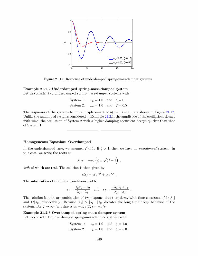
0 5 10 15 20

−1

−0.5

0

0.5

1

t

u

ωn=1.00, ζ=0.10

ωn=1.00, ζ=0.50

Figure 21.17: Response of underdamped spring-mass-damper systems.

Example 21.2.2 Underdamped spring-mass-damper systemLet us consider two underdamped spring-mass-damper systems with

System 1: ωn = 1.0 and ζ = 0.1

System 2: ωn = 1.0 and ζ = 0.5 .

The responses of the systems to initial displacement of u(t = 0) = 1.0 are shown in Figure 21.17.Unlike the undamped systems considered in Example 21.2.1, the amplitude of the oscillations decayswith time; the oscillation of System 2 with a higher damping coefficient decays quicker than thatof System 1.

·

Homogeneous Equation: Overdamped

In the underdamped case, we assumed ζ < 1. If ζ > 1, then we have an overdamped system. Inthis case, we write the roots as

λ1,2 = −ωn(ζ ±

√ζ2 − 1

),

both of which are real. The solution is then given by

u(t) = c1eλ1t + c2e

λ2t .

The substitution of the initial conditions yields

c1 =λ2u0 − v0

λ2 − λ1and c2 =

−λ1u0 + v0

λ2 − λ1.

The solution is a linear combination of two exponentials that decay with time constants of 1/|λ1|and 1/|λ2|, respectively. Because |λ1| > |λ2|, |λ2| dictates the long time decay behavior of thesystem. For ζ →∞, λ2 behaves as −ωn/(2ζ) = −k/c.Example 21.2.3 Overdamped spring-mass-damper systemLet us consider two overdamped spring-mass-damper systems with

System 1: ωn = 1.0 and ζ = 1.0

System 2: ωn = 1.0 and ζ = 5.0 .

349

0 5 10 15 20

−1

−0.5

0

0.5

1

t

u

ωn=1.00, ζ=1.00

ωn=1.00, ζ=5.00

Figure 21.18: Response of overdamped spring-mass-damper systems.

The responses of the systems to initial displacement of u(t = 0) = 1.0 are shown in Figure 21.17.As the systems are overdamped, they exhibit non-oscillatory behaviors. Note that the oscillationof System 2 with a higher damping coefficient decays more slowly than that of System 1. This isin contrast to the underdamped cases considered in Example 21.2.2, in which the oscillation of thesystem with a higher damping coefficient decays more quickly.

·

Sinusoidal Forcing

Let us consider a sinusoidal forcing of the second-order system. In particular, we consider a systemof the form

md2u

dt2+ c

du

dt+ ku = A cos(ωt) .

In terms of the natural frequency and the damping ratio previously defined, we can rewrite thesystem as

d2u

dt2+ 2ζωn

du

dt+ ω2

nu =A

mcos(ωt) .

A particular solution is of the form

up(t) = α cos(ωt) + β sin(ωt) .

Substituting the assumed form of particular solution into the governing equation, we obtain

0 =d2updt2

+ 2ζωndupdt

+ ω2nup −

A

mcos(ωt)

= − αω2 cos(ωt)− βω2 sin(ωt) + 2ζωn(−αω sin(ωt) + βω cos(ωt))

+ ω2n(α cos(ωt) + β sin(ωt))−A cos(ωt) .

350

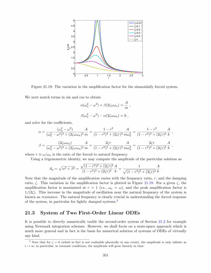
0 0.5 1 1.5 2 2.5 30

0.5

1

1.5

2

2.5

3

3.5

4

4.5

5

r

Apk/A

ζ=0.01

ζ=0.1

ζ=0.2

ζ=0.3

ζ=0.5

ζ=1

Figure 21.19: The variation in the amplification factor for the sinusoidally forced system.

We next match terms in sin and cos to obtain

α(ω2n − ω2) + β(2ζωωn) =

A

m,

β(ω2n − ω2)− α(2ζωωn) = 0 ,

and solve for the coefficients,

α =(ω2n − ω2)

(ω2n − ω2)2 + (2ζωωn)2

A

m=

1− r2

(1− r2)2 + (2ζr)2

A

mω2n

=1− r2

(1− r2)2 + (2ζr)2

A

k,

β =(2ζωωn)

(ω2n − ω2)2 + (2ζωωn)2

A

m=

2ζr

(1− r2)2 + (2ζr)2

A

mω2n

=2ζr

(1− r2)2 + (2ζr)2

A

k,

where r ≡ ω/ωn is the ratio of the forced to natural frequency.Using a trigonometric identity, we may compute the amplitude of the particular solution as

Ap =√α2 + β2 =

√(1− r2)2 + (2ζr)2

(1− r2)2 + (2ζr)2

A

k=

1√(1− r2)2 + (2ζr)2

A

k.

Note that the magnitude of the amplification varies with the frequency ratio, r, and the dampingratio, ζ. This variation in the amplification factor is plotted in Figure 21.19. For a given ζ, theamplification factor is maximized at r = 1 (i.e., ωn = ω), and the peak amplification factor is1/(2ζ). This increase in the magnitude of oscillation near the natural frequency of the system isknown as resonance. The natural frequency is clearly crucial in understanding the forced responseof the system, in particular for lightly damped systems.3

21.3 System of Two First-Order Linear ODEs

It is possible to directly numerically tackle the second-order system of Section 21.2 for exampleusing Newmark integration schemes. However, we shall focus on a state-space approach which ismuch more general and in fact is the basis for numerical solution of systems of ODEs of virtuallyany kind.

3 Note that for ζ = 0 (which in fact is not realizable physically in any event), the amplitude is only infinite ast→∞; in particular, in resonant conditions, the amplitude will grow linearly in time.

351

21.3.1 State Space Representation of Scalar Second-Order ODEs

In this section, we develop a state space representation of the canonical second-order ODE. Recallthat the ODE of interest is of the form

d2u

dt2+ 2ζωn

du

dt+ ω2

nu =1

mf(t), 0 < t < tf ,

u(0) = u0 ,

du

dt(0) = v0 .

Because this is a second-order equation, we need two variables to fully describe the state of thesystem. Let us choose these state variables to be

w1(t) = u(t) and w2(t) =du

dt(t) ,

corresponding to the displacement and velocity, respectively. We have the trivial relationshipbetween w1 and w2

dw1

dt=du

dt= w2 .

Furthermore, the governing second-order ODE can be rewritten in terms of w1 and w2 as

dw2

dt=

d

dt

du

dt=d2u

dt2− 2ζωn

du

dt= −ω2

nu+1

mf = −2ζωnw2 − ω2

nw1 +1

mf .

Together, we can rewrite the original second-order ODE as a system of two first-order ODEs,-

d

dt

(w1

w2

)=

(w2

−ω2nw1 − 2ζωnw2 + 1

m f

).

This equation can be written in the matrix form

d

dt

(w1

w2

)=

(0 1

−ω2n −2ζωn

)︸ ︷︷ ︸

A

(w1

w2

)+

(0

1m f

)(21.2)

with the initial condition

w1(0) = u0 and w2(0) = v0 .

If we define w = (w1 w2)T and F = (0 1mf)T, then

dw

dt= Aw + F, w(t = 0) = w0 =

(u0

v0

), (21.3)

succinctly summarizes the “state-space” representation of our ODE.

352

Solution by Modal Expansion

To solve this equation, we first find the eigenvalues of A. We recall that the eigenvalues are theroots of the characteristic equation p(λ;A) = det(λI−A), where det refers to the determinant. (Inactual practice for large systems the eigenvalues are not computed from the characteristic equation.In our 2× 2 case we obtain

p(λ;A) = det(λI −A) = det

(λ −1

ω2n λ+ 2ζωn

)= λ2 + 2ζωnλ+ ω2

n .

The eigenvalues, the roots of characteristic equation, are thus

λ1,2 = −ζωn ± ωn√ζ2 − 1 .

We shall henceforth assume that the system is underdamped (i.e., ζ < 1), in which case it is moreconvenient to express the eigenvalues as

λ1,2 = −ζωn ± iωn√

1− ζ2 .

Note since the eigenvalue has non-zero imaginary part the solution will be oscillatory and since thereal part is negative (left-hand of the complex plane) the solution is stable. We now consider theeigenvectors.

Towards that end, we first generalize our earlier discussion of vectors of real-valued componentsto the case of vectors of complex-valued components. To wit, if we are given two vectors v ∈ Cm×1,w ∈ Cm×1 — v and w are each column vectors with m complex entries — the inner product is nowgiven by

β = vHw =m∑j=1

v∗j wj , (21.4)

where β is in general complex, H stands for Hermitian (complex transpose) and replaces T fortranspose, and ∗ denotes complex conjugate — so vj = Real(vj) + i Imag(vj) and v∗j = Real(vj)−i Imag(vj), for i =

√−1.

The various concepts built on the inner product change in a similar fashion. For example,two complex-valued vectors v and w are orthogonal if vHw = 0. Most importantly, the norm ofcomplex-valued vector is now given by

‖v‖ =√vHv =

m∑j=1

v∗j vj

1/2

=

m∑j=1

|vj |21/2

, (21.5)

where | · | denotes the complex modulus; |vj |2 = v∗j vj = (Real(vj))2 + (Imag(vj))

2. Note thedefinition (21.5) of the norm ensures that ‖v‖ is a non-negative real number, as we would expectof a length.

To obtain the eigenvectors, we must find a solution to the equation

(λI −A)χ = 0 (21.6)

for λ = λ1 (⇒ eigenvector χ1 ∈ C2) and λ = λ2 (⇒ eigenvector χ2 ∈ C2). The equations (21.6)will have a solution since λ has been chosen to make (λI −A) singular: the columns of λI −A arenot linearly independent, and hence there exists a (in fact, many) nontrivial linear combination,χ 6= 0, of the columns of λI −A which yields the zero vector.

353

Proceeding with the first eigenvector, we write (λ1I −A)χ1 = 0 as −ζωn + iωn√

1− ζ2 −1

ω2n ζωn + iωn

√1− ζ2

( χ11

χ12

)=

0

0

to obtain (say, setting χ1

1 = c),

χ1 = c

1

−ω2n

ζωn + iωn√

1− ζ2

.

We now choose c to achieve ‖χ1‖ = 1, yielding

χ1 =1√

1 + ω2n

1

−ζωn + iωn√

1− ζ2

.

In a similar fashion we obtain from (λ2I −A)χ2 = 0 the second eigenvector

χ2 =1√

1 + ω2n

1

−ζωn − iωn√

1− ζ2

,

which satisfies ‖χ2‖ = 1.We now introduce two additional vectors, ψ1 and ψ2. The vector ψ1 is chosen to satisfy

(ψ1)Hχ2 = 0 and (ψ1)Hχ1 = 1, while the vector ψ2 is chosen to satisfy (ψ2)Hχ1 = 0 and (ψ2)Hχ2 =1. We find, after a little algebra,

ψ1 =

√1 + ω2

n

2iωn√

1− ζ2

−ζωn + iωn√

1− ζ2

−1

, ψ2 =

√1 + ω2

n

−2iωn√

1− ζ2

−ζωn − iωn√1− ζ2

−1

.

These choices may appear mysterious, but in a moment we will see the utility of this “bi-orthogonal”system of vectors. (The steps here in fact correspond to the “diagonalization” of A.)

We now write w as a linear combination of the two eigenvectors, or “modes,”

w(t) = z1(t) χ1 + z2(t) χ2

= S z(t) (21.7)

whereS = (χ1 χ2)

is the 2× 2 matrix whose jth-column is given by the jth-eigenvector, χj . We next insert (21.7) into(21.3) to obtain

χ1 dz1

dt+ χ2dz2

dt= A(χ1z1 + χ2z2) + F , (21.8)

(χ1z1 + χ2z2)(t = 0) = w0 . (21.9)

We now take advantage of the ψ vectors.

354

First we multiply (21.8) by (ψ1)H and take advantage of (ψ1)H χ2 = 0, (ψ1)H χ1 = 1, andAχj = λjχ

j to obtaindz1

dt= λ1 z1 + (ψ1)H F ; (21.10)

if we similarly multiply (21.9) we obtain

z1(t = 0) = (ψ1)H w0 . (21.11)

The same procedure but now with (ψ2)H rather than (ψ1)H gives

dz2

dt= λ2 z2 + (ψ2)H F ; (21.12)

z2(t = 0) = (ψ2)H w0 . (21.13)

We thus observe that our modal expansion reduces our coupled 2×2 ODE system into two decoupledODEs.

The fact that λ1 and λ2 are complex means that z1 and z2 are also complex, which might appearinconsistent with our original real equation (21.3) and real solution w(t). However, we note thatλ2 = λ∗1 and ψ2 = (ψ1)∗ and thus z2 = z∗1 . It thus follows from (21.7) that, since χ2 = (χ1)∗ aswell,

w = z1χ1 + z∗1(χ1)∗ ,

and thusw = 2 Real(z1χ

1) .

Upon superposition, our solution is indeed real, as desired.It is possible to use this modal decomposition to construct numerical procedures. However, our

interest here in the modal decomposition is as a way to understand how to choose an ODE schemefor a system of two (later n) ODEs, and, for the chosen scheme, how to choose ∆t for stability.

21.3.2 Numerical Approximation of a System of Two ODEs

Crank-Nicolson

The application of the Crank-Nicolson scheme to our system (21.3) is identical to the application ofthe Crank-Nicolson scheme to a scalar ODE. In particular, we directly take the scheme of example21.1.8 and replace uj ∈ R with wj ∈ R2 and g with Awj + F j to obtain

wj = wj−1 +∆t

2(Awj +Awj−1) +

∆t

2(F j + F j−1) . (21.14)

(Note if our force f is constant in time then F j = F .) In general if follows from consistencyarguments that we will obtain the same order of convergence as for the scalar problem — if (21.14)is stable. The difficult issue for systems is stability : Will a particular scheme have good stabilityproperties for a particular equation (e.g., our particular A of (21.2))? And for what ∆t will thescheme be stable? (The latter is particularly important for explicit schemes.)

To address these questions we again apply modal analysis but now to our discrete equations(21.14). In particular, we write

wj = zj1χ1 + zj2χ

2 , (21.15)

355

where χ1 and χ2 are the eigenvectors of A as derived in the previous section. We now insert (21.15)into (21.14) and multiply by (ψ1)H and (ψ2)H — just as in the previous section — to obtain

zj1 = zj−11 +

λ1∆t

2(zj1 + zj−1

1 ) + (ψ1)H ∆t

2(F j + F j−1) , (21.16)

zj2 = zj−12 +

λ2∆t

2(zj2 + zj−1

2 ) + (ψ2)H ∆t

2(F j + F j−1) , (21.17)

with corresponding initial conditions (which are not relevant to our current discussion).We now recall that for the model problem

du

dt= λu+ f , (21.18)

analogous to (21.10), we arrive at the Crank-Nicolson scheme

uj = uj−1 +λ∆t

2(uj + uj−1) +

∆t

2(f j + f j−1) , (21.19)

analogous to (21.16). Working backwards, for (21.19) and hence (21.16) to be a stable approx-imation to (21.18) and hence (21.10), we must require λ∆t, and hence λ1∆t, to reside in theCrank-Nicolson absolute stability region depicted in Figure 21.12(a). Put more bluntly, we knowthat the difference equation (21.16) will blow up — and hence also (21.14) by virture of (21.15)— if λ1∆t is not in the unshaded region of Figure 21.12(a). By similar arguments, λ2∆t must alsolie in the unshaded region of Figure 21.12(a). In this case, we know that both λ1 and λ2 — forour particular equation, that is, for our particular matrix A (which determines the eigenvalues λ1,λ2) — are in the left-hand plane, and hence in the Crank-Nicolson absolute stability region; thusCrank-Nicolson is unconditionally stable — stable for all ∆t — for our particular equation and willconverge as O(∆t2) as ∆t→ 0.

We emphasize that the numerical procedure is given by (21.14) , and not by (21.16), (21.17).The modal decomposition is just for the purposes of understanding and analysis — to determine if ascheme is stable and if so for what values of ∆t. (For a 2×2 matrix A the full modal decomposition issimple. But for larger systems, as we will consider in the next section, the full modal decompositionis very expensive. Hence we prefer to directly discretize the original equation, as in (21.14). Thisdirect approach is also more general, for example for treatment of nonlinear problems.) It followsthat ∆t in (21.16) and (21.17) are the same — both originate in the equation (21.14). We discussthis further below in the context of stiff equations.

General Recipe

We now consider a general system of n = 2 ODEs given by

dw

dt= Aw + F ,

w(0) = w0 ,

(21.20)

where w ∈ R2, A ∈ R2×2 (a 2× 2 matrix), F ∈ R2, and w0 ∈ R2. We next discretize (21.20) by anyof the schemes developed earlier for the scalar equation

du

dt= g(u, t)

356

simply by substituting w for u and Aw + F for g(u, t). We shall denote the scheme by S and theassociated absolute stability region by RS. Recall that RS is the subset of the complex plane whichcontains all λ∆t for which the scheme S applied to g(u, t) = λu is absolutely stable.

For example, if we apply the Euler Forward scheme S we obtain

wj = wj−1 + ∆t(Awj−1 + F j−1) , (21.21)

whereas Euler Backward as S yields

wj = wj−1 + ∆t(Awj + F j) , (21.22)

and Crank-Nicolson as S gives

wj = wj−1 +∆t

2(Awj +Awj−1) +

∆t

2(F j + F j−1) . (21.23)

A multistep scheme such as AB2 as S gives

wj = wj−1 + ∆t

(3

2Awj−1 − 1

2Awj−2

)+ ∆t

(3

2F j−1 − 1

2F j−2

). (21.24)

The stability diagrams for these four schemes, RS, are given by Figure 21.9, Figure 21.7, Fig-ure 21.12(a), and Figure 21.11(b), respectively.

We next assume that we can calculate the two eigenvalues of A, λ1, and λ2. A particular ∆twill lead to a stable scheme if and only if the two points λ1∆t and λ2∆t both lie inside RS. If eitheror both of the two points λ1∆t or λ2∆t lie outside RS, then we must decrease ∆t until both λ1∆tand λ2∆t lie inside RS. The critical time step, ∆tcr, is defined to be the largest ∆t for which thetwo rays [0, λ1∆t], [0, λ2∆t], both lie within RS; ∆tcr will depend on the shape and size of RS andthe “orientation” of the two rays [0, λ1∆t], [0, λ2∆t].

We can derive ∆tcr in a slightly different fashion. We first define ∆t1 to be the largest ∆t suchthat the ray [0, λ1∆t] is in RS; we next define ∆t2 to be the largest ∆t such that the ray [0, λ2∆t]

is in RS. We can then deduce that ∆tcr = min(∆t1, ∆t2). In particular, we note that if ∆t > ∆tcr

then one of the two modes — and hence the entire solution — will explode. We can also see hereagain the difficulty with stiff equations in which λ1 and λ2 are very different: ∆t1 may be (say)

much larger than ∆t2, but ∆t2 will dictate ∆t and thus force us to take many time steps — manymore than required to resolve the slower mode (smaller |λ1| associated with slower decay or sloweroscillation) which is often the behavior of interest.

In the above we assumed, as is almost always the case, that the λ are in the left-hand plane.For any λ which are in the right-hand plane, our condition is flipped: we now must make sure thatthe λ∆t are not in the absolute stability region in order to obtain the desired growing (unstable)solutions.

Let us close this section with two examples.

Example 21.3.1 Undamped spring-mass systemIn this example, we revisit the undamped spring-mass system considered in the previous section.The two eigenvalues of A are λ1 = iωn and λ2 = iωn; without loss of generality, we set ωn = 1.0.We will consider application of several different numerical integration schemes to the problem; foreach integrator, we assess its applicability based on theory (by appealing to the absolute stabilitydiagram) and verify our assessment through numerical experiments.

(i) Euler Forward is a poor choice since both λ1∆t and λ2∆t are outside RS=EF for all ∆t. Theresult of numerical experiment, shown in Figure 21.20(a), confirms that the amplitude of theoscillation grows for both ∆t = 0.5 and ∆t = 0.025; the smaller time step results in a smaller(artificial) amplification.

357

0 5 10 15 20 25 30−1.5

−1

−0.5

0

0.5

1

1.5

t

u

∆t=0.500

∆t=0.025

exact

(a) Euler Forward

0 5 10 15 20 25 30−1.5

−1

−0.5

0

0.5

1

1.5

t

u

∆t=0.500

∆t=0.025

exact

(b) Euler Backward

0 5 10 15 20 25 30−1.5

−1

−0.5

0

0.5

1

1.5

t

u

∆t=0.500

∆t=0.025

exact

(c) Crank-Nicolson

0 5 10 15 20 25 30−1.5

−1

−0.5

0

0.5

1

1.5

t

u

∆t=0.500

∆t=0.025

exact

(d) Four-stage Runge-Kutta

Figure 21.20: Comparison of numerical integration schemes for an undamped spring-mass systemwith ωn = 1.0.

358

(ii) Euler Backward is also a poor choice since λ1∆t and λ2∆t are in the interior of RS=EB for all∆t and hence the discrete solution will decay even though the exact solution is a non-decayingoscillation. Figure 21.20(b) confirms the assessment.

(iii) Crank-Nicolson is a very good choice since λ1∆t ∈ RS=CN, λ2∆t ∈ RS=CN for all ∆t, andfurthermore λ1∆t, λ2∆t lie on the boundary of RS=CN and hence the discrete solution, justas the exact solution, will not decay. Figure 21.20(c) confirms that Crank-Nicolson preservesthe amplitude of the response regardless of the choice of ∆t; however, the ∆t = 0.5 caseresults in a noticeable phase error.

(iv) Four-stage Runge-Kutta (RK4) is a reasonably good choice since λ1∆t and λ2∆t lie closeto the boundary of RS=RK4 for |λi∆t| . 1. Figure 21.20(d) shows that, for the problemconsidered, RK4 excels at not only preserving the amplitude of the oscillation but also atattaining the correct phase.

Note in the above analysis the absolute stability diagram serves not only to determine stability butalso the nature of the discrete solution as regards growth, or decay, or even neutral stability — nogrowth or decay. (The latter does not imply that the discrete solution is exact, since in addition toamplitude errors there are also phase errors. Our Crank-Nicolson result, shown in Figure 21.20(c),in particular demonstrate the presence of phase errors in the absence of amplitude errors.)

·

Example 21.3.2 Overdamped spring-mass-damper system: a stiff system of ODEsIn our second example, we consider a (very) overdamped spring-mass-damper system with ωn = 1.0and ζ = 100. The eigenvalues associated with the system are

λ1 = −ζωn + ωn√ζ2 − 1 = −0.01

λ2 = −ζωn − ωn√ζ2 − 1 = −99.99 .

As before, we perturb the system by a unit initial displacement. The slow mode with λ1 = −0.01dictates the response of the system. However, for conditionally stable schemes, the stability isgoverned by the fast mode with λ2 = −99.99. We again consider four different time integrators:two explicit and two implicit.

(i) Euler Forward is stable for ∆t . 0.02 (i.e. ∆tcr = 2/|λ2|). Figure 21.21(a) shows thatthe scheme accurately tracks the (rather benign) exact solution for ∆t = 0.02, but becomesunstable and diverges exponentially for ∆t = 0.0201. Thus, the maximum time step is limitednot by the ability to approximate the system response (dictated by λ1) but rather by stability(dictated by λ2). In other words, even though the system response is benign, we cannot uselarge time steps to save on computational cost.

(ii) Similar to the Euler Forward case, the four-stage Runge-Kutta (RK4) scheme exhibits anexponentially diverging behavior for ∆t > ∆tcr ≈ 0.028, as shown in Figure 21.21(b). Themaximum time step is again limited by stability.

(iii) Euler Backward is unconditionally stable, and thus the choice of the time step is dictatedby the ability to approximate the system response, which is dictated by λ1. Figure 21.21(c)shows that Euler Backward in fact produces a good approximation even for a time step aslarge as ∆t = 5.0 since the system response is rather slow.

359

(iv) Crank-Nicolson is also unconditionally stable. For the same set of time steps, Crank-Nicolsonproduces a more accurate approximation than Euler Backward, as shown in Figure 21.21(d),due to its higher-order accuracy.

In the above comparison, the unconditionally stable schemes required many fewer time steps(and hence much less computational effort) than conditionally stable schemes. For instance, Crank-Nicolson with ∆t = 5.0 requires approximately 200 times fewer time steps than the RK4 scheme(with a stable choice of the time step). More importantly, as the shortest time scale (i.e. the largesteigenvalue) dictates stability, conditionally stable schemes do not allow the user to use large timesteps even if the fast modes are of no interest to the user . As mentioned previously, stiff systems areubiquitous in engineering, and engineers are often not interested in the smallest time scale presentin the system. (Recall the example of the time scale associated with the dynamics of a passengerjet and that associated with turbulent eddies; engineers are often only interested in characterizingthe dynamics of the aircraft, not the eddies.) In these situations, unconditionally stable schemesallow users to choose an appropriate time step independent of stability limitations.

·In closing, it is clear even from these simple examples that a general purpose explicit scheme

would ideally include some part of both the negative real axis and the imaginary axis. Schemesthat exhibit this behavior include AB3 and RK4. Of these two schemes, RK4 is often preferreddue to a large stability region; also RK4, a multi-stage method, does not suffer from the start-upissues that sometimes complicate multi-step techniques.

21.4 IVPs: System of n Linear ODEs

We consider here for simplicity a particular family of problems: n/2 coupled oscillators. This familyof systems can be described by the set of equations.

d2u(1)

dt2= h(1)

(du(j)

dt, u(j), 1 ≤ j ≤ n/2

)+ f (1)(t) ,

d2u(2)

dt2= h(2)

(du(j)

dt, u(j), 1 ≤ j ≤ n/2

)+ f (2)(t) ,

...

d2u(n/2)

dt2= h(n/2)

(du(j)

dt, u(j), 1 ≤ j ≤ n/2

)+ f (n/2)(t) ,

where h(k) is assumed to be a linear function of all its arguments.

360

0 5 10 15 20 25 300.6

0.7

0.8

0.9

1

1.1

1.2

t

u

∆t=0.0201

∆t=0.0200

exact

(a) Euler Forward

0 5 10 15 20 25 300.6

0.7

0.8

0.9

1

1.1

1.2

t

u

∆t=0.0280

∆t=0.0270

exact

(b) Four-stage Runge-Kutta

0 5 10 15 20 25 300.6

0.7

0.8

0.9

1

1.1

1.2

t

u

∆t=5.0000

∆t=0.5000

exact

(c) Euler Backward

0 5 10 15 20 25 300.6

0.7

0.8

0.9

1

1.1

1.2

t

u

∆t=5.0000

∆t=0.5000

exact

(d) Crank-Nicolson

Figure 21.21: Comparison of numerical integration schemes for an overdamped spring-mass-dampersystem with ωn = 1.0 and ζ = 50. Note that the time step used for the explicit schemes are differentfrom those for the implicit schemes.

361

We first convert this system of equations to state space form. We identify

w1 = u(1), w2 =du(1)

dt,

w3 = u(2), w4 =du(2)

dt,

...

wn−1 = u(n/2), wn =du(n/2)

dt.

We can then write our system — using the fact that h is linear in its arguments — as

dw

dt= Aw + F

w(0) = w0

(21.25)

where h determines A, F is given by(

0 f (1)(t) 0 f (2)(t) . . . 0 f (n/2)(t))T

, and

w0 =

(u(1)(0)

du(1)

dt(0) u(2)(0)

du(2)

dt(0) . . . u(n/2)(0)

du(n/2)

dt(0)

)T

.

We have now reduced our problem to an abstract form identical to (21.20) and hence we may applyany scheme S to (21.25) in the same fashion as to (21.20).

For example, Euler Forward, Euler Backward, Crank-Nicolson, and AB2 applied to (21.25)will take the same form (21.21), (21.22), (21.23), (21.24), respectively, except that now w ∈ Rn,A ∈ Rn×n, F ∈ Rn, w0 ∈ Rn are given in (21.25), where n/2, the number of oscillators (or masses)in our system, is no longer restricted to n/2 = 1 (i.e., n = 2). We can similarly apply AB3 or BD2or RK4.

Our stability criterion is also readily extended. We first note that A will now have in generaln eigenvalues, λ1, λ2, . . . , λn. (In certain cases multiple eigenvalues can create difficulties; we donot consider these typically rather rare cases here.) Our stability condition is then simply stated:a time step ∆t will lead to stable behavior if and only if λi∆t is in RS for all i, 1 ≤ i ≤ n. Ifthis condition is not satisfied then there will be one (or more) modes which will explode, takingwith it (or them) the entire solution. (For certain very special initial conditions — in which the w0

is chosen such that all of the dangerous modes are initially exactly zero — this blow-up could beavoided in infinite precision; but in finite precision we would still be doomed.) For explicit schemes,∆tcr is the largest time step such that all the rays [0, λi∆t], 1 ≤ i ≤ n, lie within RS.

There are certainly computational difficulties that arise for large n that are not an issue forn = 2 (or small n). First, for implicit schemes, the necessary division — solution rather thanevaluation of matrix-vector equations — will become considerably more expensive. Second, forexplicit schemes, determination of ∆tcr, or a bound ∆tconservative

cr such that ∆tconservativecr ≈ ∆tcr

and ∆tconservativecr ≤ ∆tcr, can be difficult. As already mentioned, the full modal decomposition can

be expensive. Fortunately, in order to determine ∆tcr, we often only need as estimate for say themost negative real eigenvalue, or the largest (in magnitude) imaginary eigenvalue; these extremeeigenvalues can often be estimated relatively efficiently.

362

Finally, we note that in practice often adaptive schemes are used in which stability and accuracyare monitored and ∆t modified appropriately. These methods can also address nonlinear problems— in which h no longer depends linearly on its arguments.

363

364

Chapter 22

Boundary Value Problems

365

366

Chapter 23

Partial Differential Equations

367

368

Unit V

(Numerical) Linear Algebra 2:Solution of Linear Systems

369

Chapter 24

Motivation

We thank Dr Phuong Huynh of MIT for generously developing and sharing the robot arm model,finite element discretization, and computational results reported in this chapter.

24.1 A Robot Arm

In the earlier units we have frequently taken inspiration from applications related to robots —navigation, kinematics, and dynamics. In these earlier analyses we considered systems consistingof relatively few “lumped” components and hence the computational tasks were rather modest.However, it is also often important to address not just lumped components but also the detaileddeformations and stresses within say a robot arm: excessive deformation can compromise perfor-mance in precision applications; and excessive stresses can lead to failure in large manufacturingtasks.

The standard approach for the analysis of deformations and stresses is the finite element (FE)method. In the FE approach, the spatial domain is first broken into many (many) small regionsdenoted elements: this decomposition is often denoted a triangulation (or more generally a grid ormesh), though elements may be triangles, quadrilaterals, tetrahedra, or hexahedra; the vertices ofthese elements define nodes (and we may introduce additional nodes at say edge or face midpoints).The displacement field within each such element is then expressed in terms of a low order polyno-mial representation which interpolates the displacements at the corresponding nodes. Finally, thepartial differential equations of linear elasticity are invoked, in variational form, to yield equilibriumequations at (roughly speaking) each node in terms of the displacements at the neighboring nodes.Very crudely, the coefficients in these equations represent effective spring constants which reflectthe relative nodal geometric configuration and the material properties. We may express this systemof n equations — one equation for each node — in n unknowns — one displacement (or “degree offreedom”) for each node — as Ku = f , in which K is an n× n matrix, u is an n× 1 vector of theunknown displacements, and f is an n× 1 vector of imposed forces or “loads.”1

We show in Figure 24.1 the finite element solution for a robot arm subject only to the “self-load”induced by gravity. The blue arm is the unloaded (undeformed) arm, whereas the multi-color armis the loaded (deformed) arm; note in the latter we greatly amplify the actual displacements forpurposes of visualization. The underlying triangulation — in particular surface triangles associated

1 In fact, for this vector-valued displacement field, there are three equations and three degrees of freedom for each(geometric) node. For simplicity we speak of (generalized) nodes equated to degrees of freedom.

371

DRAFT V2.1 © The Authors. License: Creative Commons BY-NC-SA 3.0.

Figure 24.1: Deflection of robot arm.

with volumetric tetrahedral elements — is also shown. In this FE discretization there are n = 60,030degrees of freedom (for technical reasons we do not count the nodes at the robot shoulder). The issueis thus how to effectively solve the linear system of equations Ku = f given the very large numberof degrees of freedom. In fact, many finite element discretizations result not in 105 unknowns butrather 106 or even 107 unknowns. The computational task is thus formidable, in particular sincetypically one analysis will not suffice — rather, many analyses will be required for purposes ofdesign and optimization.

24.2 Gaussian Elimination and Sparsity

If we were to consider the most obvious tactic — find K−1 and then compute K−1f — the resultwould be disastrous: days of computing (if the calculation even completed). And indeed even ifwe were to apply a method of choice — Gaussian elimination (or LU decomposition) — withoutany regard to the actual structure of the matrix K, the result would still be disastrous. Moderncomputational solution strategies must and do take advantage of a key attribute ofK — sparseness.2

In short, there is no reason to perform operations which involve zero operands and will yield zerofor a result. In MechE systems sparseness is not an exceptional attribute but rather, and veryfortunately, the rule: the force in a (Hookean) spring is just determined by the deformationsof nearest neighbors, not by distant neighbors; similar arguments apply in heat transfer, fluidmechanics, and acoustics. (Note this is not to say that the equilibrium displacement at one nodedoes not depend on the applied forces at the other nodes; quite to the contrary, a force applied atone node will yield nonzero displacements at all the nodes of the system. We explore this nuancemore deeply when we explain why formation of the inverse of a (sparse) matrix is a very poor idea.)

We present in Figure 24.2 the structure of the matrix K: the dots indicate nonzero entriesin the matrix. We observe that most of the matrix elements are in fact zero. Indeed, of the3,603,600,900 entries of K, 3,601,164,194 entries are zero; put differently, there are only 2,436,706

2Note in this unit we shall consider only direct solution methods; equally important, but more advanced in termsof formulation, analysis, and robust implementation (at least if we consider the more efficient varieties), are iterativesolution methods. In actual practice, most state-of-the-art solvers include some combination of direct and iterativeaspects. And in all cases, sparsity plays a key role.

372

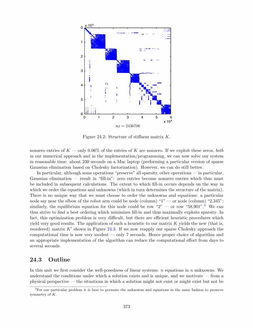
0

1

2

3

4

5

6

x 104

0 1 2 3 4 5 6x 104

Figure 24.2: Structure of stiffness matrix K.

nonzero entries of K — only 0.06% of the entries of K are nonzero. If we exploit these zeros, bothin our numerical approach and in the implementation/programming, we can now solve our systemin reasonable time: about 230 seconds on a Mac laptop (performing a particular version of sparseGaussian elimination based on Cholesky factorization). However, we can do still better.

In particular, although some operations “preserve” all sparsity, other operations — in particular,Gaussian elimination — result in “fill-in”: zero entries become nonzero entries which thus mustbe included in subsequent calculations. The extent to which fill-in occurs depends on the way inwhich we order the equations and unknowns (which in turn determines the structure of the matrix).There is no unique way that we must choose to order the unknowns and equations: a particularnode say near the elbow of the robot arm could be node (column) “1” — or node (column) “2,345”;similarly, the equilibrium equation for this node could be row “2” — or row “58,901”.3 We canthus strive to find a best ordering which minimizes fill-in and thus maximally exploits sparsity. Infact, this optimization problem is very difficult, but there are efficient heuristic procedures whichyield very good results. The application of such a heuristic to our matrix K yields the new (that is,reordered) matrix K ′ shown in Figure 24.3. If we now reapply our sparse Cholesky approach thecomputational time is now very modest — only 7 seconds. Hence proper choice of algorithm andan appropriate implementation of the algorithm can reduce the computational effort from days toseveral seconds.

24.3 Outline

In this unit we first consider the well-posedness of linear systems: n equations in n unknowns. Weunderstand the conditions under which a solution exists and is unique, and we motivate — from aphysical perspective — the situations in which a solution might not exist or might exist but not be

3For our particular problem it is best to permute the unknowns and equations in the same fashion to preservesymmetry of K.

373

0

1

2

3

4

5

6

x 104

0 1 2 3 4 5 6x 104

Figure 24.3: Structure of reordered stiffness matrix K ′.

unique.We next consider the basic Gaussian eliminate algorithm. We then proceed to Gaussian elimi-

nation for sparse systems — motivated by the example and numerical results presented above forthe robot arm. Finally, we consider the Matlab implementation of these approaches. (Note thatall results in this chapter are based on Matlab implementations.)

We notably omit several important topics: we do not consider iterative solution procedures; wedo not consider, except for a few remarks, the issue of numerical stability and conditioning.

374

Chapter 25

Linear Systems

25.1 Model Problem: n = 2 Spring-Mass System in Equilibrium

25.1.1 Description

We will introduce here a simple spring-mass system, shown in Figure 25.1, which we will usethroughout this chapter to illustrate various concepts associated with linear systems and associatedsolution techniques. Mass 1 has mass m1 and is connected to a stationary wall by a spring withstiffness k1. Mass 2 has mass of m2 and is connected to the mass m1 by a spring with stiffness k2.

We denote the displacements of mass 1 and mass 2 by u1 and u2, respectively: positive valuescorrespond to displacement away from the wall; we choose our reference such that in the absenceof applied forces — the springs unstretched — u1 = u2 = 0. We next introduce (steady) forcesf1 and f2 on mass 1 and mass 2, respectively; positive values correspond to force away from thewall. We are interested in predicting the equilibrium displacements of the two masses, u1 and u2,for prescribed forces f1 and f2.

We note that while all real systems are inherently dissipative and therefore are characterized notjust by springs and masses but also dampers, the dampers (or damping coefficients) do not affectthe system at equilibrium — since d/dt vanishes in the steady state — and hence for equilibriumconsiderations we may neglect losses. Of course, it is damping which ensures that the systemultimately achieves a stationary (time-independent) equilibrium.1

wall

k

k

1

1

f

f

1

1

u

u

1

1

m

m

1

1

f

f

2

2

u

u

2

2

m

m

2

2

k

k

2

2

“free”

Figure 25.1: A system of two masses and two springs anchored to a wall and subject to appliedforces.

1In some rather special cases — which we will study later in this chapter — the equilibrium displacement is indeedaffected by the initial conditions and damping. This special case in fact helps us better understand the mathematicalaspects of systems of linear equations.

375

DRAFT V2.1 © The Authors. License: Creative Commons BY-NC-SA 3.0.

wall

kk11

mm11 mm22

kk22

applied force on mass 1:1: (+)(+)ff11

uu22 −− uu11spring stretched

1:1: kk22((uu22 −− uu11))force on mass⇓

spring stretched uu11

1:1:−−kk11 uu11force on mass⇓

Figure 25.2: Forces on mass 1.

mm11

kk22

applied force on mass 2:2: (+)(+)ff22

uu22 −− uu11spring stretched ⇓

mm22

2:2:force on mass kk22((uu22 −− uu11))−−

Figure 25.3: Forces on mass 2.

We now derive the equations which must be satisfied by the displacements u1 and u2 at equilib-rium. We first consider the forces on mass 1, as shown in Figure 25.2. Note we apply here Hooke’slaw — a constitutive relation — to relate the force in the spring to the compression or extensionof the spring. In equilibrium the sum of the forces on mass 1 — the applied forces and the forcesdue to the spring — must sum to zero, which yields

f1 − k1 u1 + k2(u2 − u1) = 0 .

(More generally, for a system not in equilibrium, the right-hand side would be m1u1 rather thanzero.) A similar identification of the forces on mass 2, shown in Figure 25.3, yields for force balance

f2 − k2(u2 − u1) = 0 .

This completes the physical statement of the problem.Mathematically, our equations correspond to a system of n = 2 linear equations, more precisely,

2 equations in 2 unknowns:

(k1 + k2)u1 − k2 u2 = f1 , (25.1)

−k2 u1 + k2 u2 = f2 . (25.2)

Here u1 and u2 are unknown, and are placed on the left-hand side of the equations, and f1 and f2 areknown, and placed on the right-hand side of the equations. In this chapter we ask several questionsabout this linear system — and more generally about linear systems of n equations in n unknowns.First, existence: when do the equations have a solution? Second, uniqueness: if a solution exists, isit unique? Although these issues appear quite theoretical in most cases the mathematical subtletiesare in fact informed by physical (modeling) considerations. In later chapters in this unit we willask a more obviously practical issue: how do we solve systems of linear equations efficiently?

But to achieve these many goals we must put these equations in matrix form in order to besttake advantage of both the theoretical and practical machinery of linear algebra. As we have already

376

addressed the translation of sets of equations into corresponding matrix form in Unit III (relatedto overdetermined systems), our treatment here shall be brief.

We write our two equations in two unknowns as Ku = f , where K is a 2×2 matrix, u = (u1 u2)T

is a 2× 1 vector, and f = (f1 f2)T is a 2× 1 vector. The elements of K are the coefficients of theequations (25.1) and (25.2):

unknown knownk1 + k2 −k2

−k2 k2

u1

u2

=

f1

f2

· · ·← Equation (25.1)

← Equation (25.2)

K u f

2× 2 2× 1 2× 1

.(25.3)

We briefly note the connection between equations (25.3) and (25.1). We first note that Ku = Fimplies equality of the two vectors Ku and F and hence equality of each component of Ku andF . The first component of the vector Ku, from the row interpretation of matrix multiplication,2

is given by (k1 + k2)u1 − k2u2; the first component of the vector F is of course f1. We thusconclude that (Ku)1 = f1 correctly produces equation (25.1). A similar argument reveals that the(Ku)2 = f2 correctly produces equation (25.2).

25.1.2 SPD Property

We recall that a real n× n matrix A is Symmetric Positive Definite (SPD) if A is symmetric

AT = A , (25.4)

and A is positive definitevTAv > 0 for any v 6= 0 . (25.5)

Note in equation (25.5) that Av is an n× 1 vector and hence vT(Av) is a scalar — a real number.Note also that the positive definite property (25.5) implies that if vTAv = 0 then v must be the zerovector. There is also a connection to eigenvalues: symmetry implies real eigenvalues, and positivedefinite implies strictly positive eigenvalues (and in particular, no zero eigenvalues).

There are many implications of the SPD property, all very pleasant. In the context of thecurrent unit, an SPD matrix ensures positive eigenvalues which in turn will ensure existence anduniqueness of a solution — which is the topic of the next section. Furthermore, an SPD matrixensures stability of the Gaussian elimination process — the latter is the topic in the followingchapters. We also note that, although in this unit we shall focus on direct solvers, SPD matricesalso offer advantages in the context of iterative solvers: the very simple and efficient conjugategradient method can be applied (only to) SPD matrices. The SPD property is also the basis ofminimization principles which serve in a variety of contexts. Finally, we note that the SPD propertyis often, though not always, tied to a natural physical notion of energy.

We shall illustrate the SPD property for our simple 2× 2 matrix K associated with our springsystem. In particular, we now again consider our system of two springs and two masses but nowwe introduce an arbitrary imposed displacement vector v = (v1 v2)T, as shown in Figure 25.4. Inthis case our matrix A is given by K where

2In many, but not all, cases it is more intuitive to develop matrix equations from the row interpretation of matrixmultiplication; however, as we shall see, the column interpretation of matrix multiplication can be very importantfrom the theoretical perspective.

377

wall

kk11

vv11 vv22

kk22v =

(v1

v2

)any “imposed” displacement

Figure 25.4: Spring-mass system: imposed displacements v.

K =

(k1 + k2 −k2

−k2 k2

).

We shall assume that k1 > 0 and k2 > 0 — our spring constants are strictly positive. We shallreturn to this point shortly.

We can then form the scalar vTKv as

vTKv = vT

(k1 + k2 −k2

−k2 k2

)(v1

v2

)︸ ︷︷ ︸

= (v1 v2)

((k1 + k2)v1 −k2v2

−k2v1 k2v2

)︸ ︷︷ ︸

Kv

= v21(k1 + k2)− v1v2k2 − v2v1k2 + v2

2k2

= v21k1 +

(v2

1 − 2v1v2 + v22

)k2

= k1v21 + k2(v1 − v2)2 .

We now inspect this result.In particular, we may conclude that, under our assumption of positive spring constants, vTKv ≥

0. Furthermore, vTKv can only be zero if v1 = 0 and v1 = v2, which in turn implies that vTKvcan only be zero if both v1 and v2 are zero — v = 0. We thus see that K is SPD: vTKv > 0 unlessv = 0 (in which case of course vTKv = 0). Note that if either k1 = 0 or k2 = 0 then the matrix isnot SPD: for example, if k1 = 0 then vTKv = 0 for any v = (c c)T, c a real constant; similarly, ifk2 = 0, then vTKv = 0 for any v = (0 c)T, c a real constant.

We can in this case readily identify the connection between the SPD property and energy. Inparticular, for our spring system, the potential energy in the spring system is simply 1

2vTKv:

PE (potential/elastic energy) =

1

2k1v

21︸ ︷︷ ︸

energy inspring 1

+1

2k2(v2 − v1)2︸ ︷︷ ︸

energy inspring 2

=1

2vTAv > 0 (unless v = 0) ,

where of course the final conclusion is only valid for strictly positive spring constants.

378

Finally, we note that many MechE systems yield models which in turn may be described by SPDsystems: structures (trusses, . . . ); linear elasticity; heat conduction; flow in porous media (Darcy’sLaw); Stokes (or creeping) flow of an incompressible fluid. (This latter is somewhat complicatedby the incompressibility constraint.) All these systems are very important in practice and indeedubiquitous in engineering analysis and design. However, it is also essential to note that many othervery important MechE phenomena and systems — for example, forced convection heat transfer,non-creeping fluid flow, and acoustics — do not yield models which may be described by SPDmatrices.

25.2 Existence and Uniqueness: n = 2

25.2.1 Problem Statement

We shall now consider the existence and uniqueness of solutions to a general system of (n =) 2equations in (n =) 2 unknowns. We first introduce a matrix A and vector f as

2× 2 matrix A =

A11 A12

A21 A22

2× 1 vector f =

f1

f2

;

our equation for the 2× 1 unknown vector u can then be written as

Au = f , or

A11 A12

A21 A22

u1

u2

=

f1

f2

, orA11u1 +A12u2 = f1

A21u1 +A22u2 = f2

.

Note these three expressions are equivalent statements proceeding from the more abstract to themore concrete. We now consider existence and uniqueness; we shall subsequently interpret ourgeneral conclusions in terms of our simple n = 2 spring-mass system.

25.2.2 Row View

We first consider the row view, similar to the row view of matrix multiplication. In this perspectivewe consider our solution vector u = (u1 u2)T as a point (u1, u2) in the two dimensional Cartesianplane; a general point in the plane is denoted by (v1, v2) corresponding to a vector (v1 v2)T. Inparticular, u is the particular point in the plane which lies both on the straight line described bythe first equation, (Av)1 = f1, denoted ‘eqn1’ and shown in Figure 25.5 in blue, and on the straightline described by the second equation, (Av)2 = f2, denoted ‘eqn2’ and shown in Figure 25.5 ingreen.

We directly observe three possibilities, familiar from any first course in algebra; these threecases are shown in Figure 25.6. In case (i), the two lines are of different slope and there is clearlyone and only one intersection: the solution thus exists and is furthermore unique. In case (ii) thetwo lines are of the same slope and furthermore coincident: a solution exists, but it is not unique— in fact, there are an infinity of solutions. This case corresponds to the situation in which thetwo equations in fact contain identical information. In case (iii) the two lines are of the same slopebut not coincident: no solution exists (and hence we need not consider uniqueness). This casecorresponds to the situation in which the two equations contain inconsistent information.

379

uu ==uu11

uu22

vv11

vv22

eqn 11

AA1111vv11++AA1212vv22 == ff11

or vv22 ==ff11

AA1212−− AA1111

AA1212vv11

AA2121vv11++AA2222vv22 == ff22

or vv22 ==ff22

AA2222−− AA2121

AA2222vv11

eqn 22

Figure 25.5: Row perspective: u is the intersection of two straight lines.

eqn 11

eqn 22eqn 11,, eqn 22all points on line satisfy both

eqn 11

eqn 22

no points satisfy both

(i) (ii) (iii)

exists 3 exists 3 exists 7

unique 3 unique 7 ����unique

redundant information, inconsistent informationinfinity of solutions no solution

Figure 25.6: Three possibilities for existence and uniqueness; row interpretation.

380

pp22

uu22 pp22

ff

uu11 pp11 pp11

ff −− uu11 pp11 pp22

Figure 25.7: Parallelogram construction for the case in case in which a unique solution exists.

We see that the condition for (both) existence and uniqueness is that the slopes of ‘eqn1’ and‘eqn2’ must be different, or A11/A12 6= A21/A22, or A11A22 − A12A21 6= 0. We recognize the latteras the more familiar condition det(A) 6= 0. In summary, if det(A) 6= 0 then our matrix A is non-singular and the system Au = f has a unique solution; if det(A) 6= 0 then our matrix A is singularand either our system has an infinity of solutions or no solution, depending on f . (In actual practicethe determinant condition is not particularly practical computationally, and serves primarily as aconvenient “by hand” check for very small systems.) We recall that a non-singular matrix A hasan inverse A−1 and hence in case (i) we can write u = A−1f ; we presented this equation earlierunder the assumption that A is non-singular — now we have provided the condition under whichthis assumption is true.

25.2.3 The Column View

We next consider the column view, analogous to the column view of matrix multiplication. Inparticular, we recall from the column view of matrix-vector multiplication that we can express Auas

Au =

A11 A12

A21 A22

u1

u2

=

A11

A21

u1 +

A12

A22

u2

︸ ︷︷ ︸p1

︸ ︷︷ ︸p2

,

where p1 and p2 are the first and second column of A, respectively. Our system of equations canthus be expressed as

Au = f ⇔ p1u1 + p2u2 = f .

Thus the question of existence and uniqueness can be stated alternatively: is there a (unique?)combination, u, of columns p1 and p2 which yields f?

We start by answering this question pictorially in terms of the familiar parallelogram construc-tion of the sum of two vectors. To recall the parallelogram construction, we first consider in detailthe case shown in Figure 25.7. We see that in the instance depicted in Figure 25.7 there is clearlya unique solution: we choose u1 such that f − u1p

1 is parallel to p2 (there is clearly only one suchvalue of u1); we then choose u2 such that u2p

2 = f − u1p1.

We can then identify, in terms of the parallelogram construction, three possibilities; these threecases are shown in Figure 25.8. Here case (i) is the case already discussed in Figure 25.7: a uniquesolution exists. In both cases (ii) and (iii) we note that

p2 = γp1 or p2 − γp1 = 0 (p1 and p2 are linearly dependent)

for some γ, where γ is a scalar; in other words, p1 and p2 are colinear — point in the same directionto within a sign (though p1 and p2 may of course be of different magnitude). We now discuss thesetwo cases in more detail.

381

pp22

ff

pp11

pp22

ff

pp11

pp22

ff

pp11*

forfor ananyy vv11

ff −− vv11pp11 ∦∦ toto pp22

(i) (ii) (iii)

exists 3 exists 3 exists 7

unique 3 unique 7 ����unique

(only p1, ormore p1 and some p2, or . . . )

Figure 25.8: Three possibilities for existence and uniqueness; the column perspective.

In case (ii), p1 and p2 are colinear but f also is colinear with p1 (and p2) — say f = βp1 forsome scalar β. We can thus write

f = p1 · β + p2 · 0

=

p1 p2

β0

=

A11 A12

A21 A22

β0

︸︷︷︸u∗

= Au∗ ,

and hence u∗ is a solution. However, we also know that −γp1 + p2 = 0, and hence

0 = p1 · (−γ) + p2 · (1)

=

p1 p2

−γ1

=

A11 A12

A21 A22

−γ1

= A

−γ1

.

Thus, for any α,

u = u∗ + α

−γ1

︸ ︷︷ ︸infinity of solutions

382

satisfies Au = f , since

A

u∗ + α

−γ1

= Au∗ +A

α−γ

1

= Au∗ + αA

−γ1

= f + α · 0

= f .

This demonstrates that in case (ii) there are an infinity of solutions parametrized by the arbitraryconstant α.

Finally, we consider case (iii). In this case it is clear from our parallelogram construction thatfor no choice of v1 will f −v1p

1 be parallel to p2, and hence for no choice of v2 can we form f −v1p1

as v2p2. Put differently, a linear combination of two colinear vectors p1 and p2 can not combine to

form a vector perpendicular to both p1 and p2. Thus no solution exists.Note that the vector (−γ 1)T is an eigenvector of A corresponding to a zero eigenvalue.3 By

definition the matrix A has no effect on an eigenvector associated with a zero eigenvalue, and it isfor this reason that if we have one solution to Au = f then we may add to this solution any multiple— here α — of the zero-eigenvalue eigenvector to obtain yet another solution. More generally amatrix A is non-singular if and only if it has no zero eigenvalues; in that case — case (i) — theinverse exists and we may write u = A−1f . On the other hand, if A has any zero eigenvalues thenA is singular and the inverse does not exist; in that case Au = f may have either many solutionsor no solutions, depending on f . From our discussion of SPD systems we also note that A SPD isa sufficient (but not necessary) condition for the existence of the inverse of A.

25.2.4 A Tale of Two Springs

We now interpret our results for existence and uniqueness for a mechanical system — our twosprings and masses — to understand the connection between the model and the mathematics. Weagain consider our two masses and two springs, shown in Figure 25.9, governed by the system ofequations

Au = f for A = K ≡

k1 + k2 −k2

−k2 k2

.

We analyze three different scenarios for the spring constants and forces, denoted (I), (II), and (III),which we will see correspond to cases (i), (ii), and (iii), respectively, as regards existence anduniqueness. We present first (I), then (III), and then (II), as this order is more physically intuitive.

(I) In scenario (I) we choose k1 = k2 = 1 (more physically we would take k1 = k2 = k forsome value of k expressed in appropriate units — but our conclusions will be the same) andf1 = f2 = 1 (more physically we would take f1 = f2 = f for some value of f expressed inappropriate units — but our conclusions will be the same). In this case our matrix A and

3All scalar multiples of this eigenvector define what is known as the right nullspace of A.

383

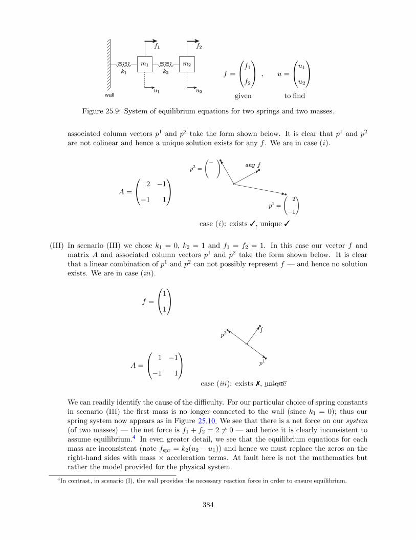
wall

kk11

ff11

uu11

mm11

ff22

uu22

mm22

kk22 f =

f1

f2

,

given

u =

u1

u2

to find

Figure 25.9: System of equilibrium equations for two springs and two masses.

associated column vectors p1 and p2 take the form shown below. It is clear that p1 and p2

are not colinear and hence a unique solution exists for any f . We are in case (i).

A =

2 −1

−1 1

p

p

2

2

=

=

−

−11

11

pp11 ==22

−−11

anyany ff

case (i): exists 3, unique 3

(III) In scenario (III) we chose k1 = 0, k2 = 1 and f1 = f2 = 1. In this case our vector f andmatrix A and associated column vectors p1 and p2 take the form shown below. It is clearthat a linear combination of p1 and p2 can not possibly represent f — and hence no solutionexists. We are in case (iii).

f =

1

1

A =

1 −1

−1 1

p

p

2

2

f

f

p

p

1

1

case (iii): exists 7,����unique

We can readily identify the cause of the difficulty. For our particular choice of spring constantsin scenario (III) the first mass is no longer connected to the wall (since k1 = 0); thus ourspring system now appears as in Figure We see that there is a net force on our system(of two masses) — the net force is f1 + f2 = 2 6= 0 — and hence it is clearly inconsistent toassume equilibrium. In even greater detail, we see that the equilibrium equations for eachmass are inconsistent (note fspr = k2(u2 − u1)) and hence we must replace the zeros on theright-hand sides with mass × acceleration terms. At fault here is not the mathematics butrather the model provided for the physical system.

4In contrast, in scenario (I), the wall provides the necessary reaction force in order to ensure equilibrium.

384

25.10.

4

mm11 mm22

kk22

ff11 == 11 ff22 == 11

ffsprspr

11 ++ ffsprspr == 00 11−− ffspsprr == 00

ffsprspr

↑↑mm11 ¨uu11 == 00 mm22 ¨uu22 == 00

(ass(assuummee sstrtreetctched)hed)

notnot pposossibsiblele

ffaultaultyy momodeldelassassuummpptiontion

↑↑

Figure 25.10: Scenario III

(II) In this scenario we choose k1 = 0, k2 = 1 and f1 = 1, f2 = −1. In this case our vector f andmatrix A and associated column vectors p1 and p2 take the form shown below. It is clearthat a linear combination of p1 and p2 now can represent f — and in fact there are manypossible combinations. We are in case (ii).

f =

−1

1

A =

1 −1

−1 1

p

p

2

2

f

f

p

p

1

1

case (ii): exists 3, unique 7

We can explicitly construct the family of solutions from the general procedure describedearlier:

p2 = = −1︸︷︷︸γ

p1 ,

f = −1︸︷︷︸β

p1 ⇒ u∗ =

= −1

0 =

⇓

u = u∗ + α

−γ1

=

−1

0

+ α

1

1

385

mm11 mm22

ff22 == 11

ffsprspr ffsprspr

(ass(assuummee sstrtreetctched)hed)

kk22 == 11

−−11 ++ ffsprspr == 00 −−ffsprspr ++ 11 == 00⇓⇓

ffsprspr == 11

11

kk22

((uu22 −− uu11)) ==⇓⇓

aa ssololutionution

ff11 == −−11

11 onlonlyy didiffffererencencee inindidisspplacelacememenntt mattersmatters

ffsprspr

Figure 25.11: Scenario II. (Note on the left mass the f1 arrow indicates the direction of the forcef1 = −1, not the direction of positive force.)

for any α. Let us check the result explicitly:

A

−1

0

+

αα

=

1 −1

−1 1

1 + α

α

=

(−1 + α)− α

(1− α) + α

=

−1

1

= f ,

as desired. Note that the zero-eigenvalue eigenvector here is given by (−γ 1)T = (1 1)T

and corresponds to an equal (or translation) shift in both displacements, which we will nowinterpret physically.

In particular, we can readily identify the cause of the non-uniqueness. For our choice of springconstants in scenario (II) the first mass is no longer connected to the wall (since k1 = 0), justas in scenario (III). Thus our spring system now appears as in Figure 25.11. But unlike inscenario (III), in scenario (II) the net force on the system is zero — f1 and f2 point in oppositedirections — and hence an equilibrium is possible. Furthermore, we see that each mass is inequilibrium for a spring force fspr = 1. Why then is there not a unique solution? Becauseto obtain fspr = 1 we may choose any displacements u such that u2 − u1 = 1 (for k2 = 1):the system is not anchored to wall — it just floats — and thus equilibrium is maintainedif we shift (or translate) both masses by the same displacement (our eigenvector) such thatthe “stretch” remains invariant. This is illustrated in Figure 25.12, in which α is the shiftin displacement. Note α is not determined by the equilibrium model; α could be determinedfrom a dynamical model and in particular would depend on the initial conditions and the

386

a solution another solution

mm11 mm22

ff22 == 11

kk22 == 11

ff11 == −−11

mm11 mm22

ff22 == 11

kk22 == 11

ff11 == −−11

u = u∗ =

−1

0

u = u∗

︸︷︷︸−1

0

+ α

1

1

︸ ︷︷ ︸αα

Figure 25.12: Scenario (II): non-uniqueness.

damping in the system.

We close this section by noting that for scenario (I) k1 > 0 and k2 > 0 and hence A (≡ K) isSPD: thus A−1 exists and Au = f has a unique solution for any forces f . In contrast, in scenarios(II) and (III), k1 = 0, and hence A is no longer SPD, and we are no longer guaranteed that A−1

exists — and indeed it does not exist. We also note that in scenario (III) the zero-eigenvalueeigenvector (1 1)T is precisely the v which yields zero energy, and indeed a shift (or translation)of our unanchored spring system does not affect the energy in the spring.

25.3 A “Larger” Spring-Mass System: n Degrees of Freedom

We now consider the equilibrium of the system of n springs and masses shown in Figure 25.13.(This string of springs and masses in fact is a model (or discretization) of a continuum truss; eachspring-mass is a small segment of the truss.) Note for n = 2 we recover the small system studiedin the preceding sections. This larger system will serve as a more “serious” model problem both asregards existence and uniqueness but even more importantly as regard computational procedures.We then consider force balance on mass 1,∑

forces on mass 1 = 0

⇒ f1 − k1u1 + k2(u2 − u1) = 0 ,

and then on mass 2, ∑forces on mass 2 = 0

⇒ f2 − k2(u2 − u1) + k3(u3 − u2) = 0 ,

and then on a typical interior mass i (hence 2 ≤ i ≤ n− 1)∑forces on mass i = 0 (i 6= 1, i 6= n)

⇒ fi − ki(ui − ui−1) + ki+1(ui+1 − ui) = 0 ,

and finally on mass n, ∑forces on mass n = 0

⇒ fn − kn(un − un−1) = 0 .

387

wall

kk11

ff11

uu11

mm11

ff22

uu22

mm22

kk22

ff33

uu33

mm33

kk33

ffnn

uunn

mmnn

kknn

…

free

Figure 25.13: System of n springs and masses.

We can write these equations as

(k1 + k2)u1 − k2u2 0 . . . = f1

− k2u1 + (k2 + k3)u2 − k3u3 0 . . . = f2

0 − k3u2 + (k3 + k4)u3 − k4u4 = f3

. . ....

. . . 0 − knun−1 + knun = fn

or

k1 + k2 −k2

−k2 k2 + k3 −k3 0−k3 k3 + k4 −k4

. . .. . .

. . .

0 −kn−kn kn

K

n× n

u1

u2

u3

...

un−1

un

u

n× 1

f1

f2

f3

...

fn−1

fn

f

n× 1

which is simply Au = f (A ≡ K) but now for n equations in n unknowns.In fact, the matrix K has a number of special properties. In particular, K is sparse — K is

mostly zero entries since only “nearest neighbor” connections affect the spring displacement andhence the force in the spring5; tri-diagonal — the nonzero entries are all on the main diagonaland diagonal just below and just above the main diagonal; symmetric — KT = K; and positivedefinite (as proven earlier for the case n = 2) — 1

2(vTKv) is the potential/elastic energy of thesystem. Some of these properties are important to establish existence and uniqueness, as discussedin the next section; some of the properties are important in the efficient computational solution ofKu = f , as discussed in the next chapters of this unit.

5This sparsity property, ubiquitous in MechE systems, will be the topic of its own chapter subsequently.

388

25.4 Existence and Uniqueness: General Case (Square Systems)

We now consider a general system of n equations in n unknowns,

A︸︷︷︸given

u︸︷︷︸to find

= f︸︷︷︸given

where A is n× n, u is n× 1, and f is n× 1.If A has n independent columns then A is non-singular, A−1 exists, and Au = f has a unique

solution u. There are in fact many ways to confirm that A is non-singular: A has n independentcolumns; A has n independent rows; A has nonzero determinant; A has no zero eigenvalues; A isSPD. (We will later encounter another condition related to Gaussian elimination.) Note all theseconditions are necessary and sufficient except the last: A is SPD is only a sufficient conditionfor non-singular A. Conversely, if any of the necessary conditions is not true then A is singularand Au = f either will have many solutions or no solution, depending of f .6 In short, all of ourconclusions for n = 2 directly extend to the case of general n.

6Note in the computational context we must also understand and accommodate “nearly” singular systems. Wedo not discuss this more advanced topic further here.

389

390

Chapter 26

Gaussian Elimination and BackSubstitution

26.1 A 2× 2 System (n = 2)

Let us revisit the two-mass mass-spring system (n = 2) considered in the previous chapter; thesystem is reproduced in Figure 26.1 for convenience. For simplicity, we set both spring constantsto unity, i.e. k1 = k2 = 1. Then, the equilibrium displacement of mass m1 and m2, u1 and u2, isdescribed by a linear system

A(K)

u = f →

2 −1

−1 1

u1

u2

=

f1

f2

, (26.1)

where f1 and f2 are the forces applied to m1 and m2. We will use this 2 × 2 system to describea systematic two-step procedure for solving a linear system: a linear solution strategy based onGaussian elimination and back substitution. While the description of the solution strategy mayappear overly detailed, we focus on presenting a systematic approach such that the approachgeneralizes to n× n systems and can be carried out by a computer.

By row-wise interpretation of the linear system, we arrive at a system of linear equations

2 u1pivot

− u2 = f1

−1u1 + u2 = f2.

wall

k

k

1

1

f

f

1

1

u

u

1

1

m

m

1

1

f

f

2

2

u

u

2

2

m

m

2

2

k

k

2

2

k1 = k2 = “1”

Figure 26.1: n = 2 spring-mass system.

391

DRAFT V2.1 © The Authors. License: Creative Commons BY-NC-SA 3.0.

We recognize that we can eliminate u1 from the second equation by adding 1/2 of the first equationto the second equation. The scaling factor required to eliminate the first coefficient from the secondequation is simply deduced by diving the first coefficient of the second equation (−1) by the “pivot”— the leading coefficient of the first equation (2) — and negating the sign; this systematic procedureyields (−(−1)/2) = 1/2 in this case. Addition of 1/2 of the first equation to the second equationyields a new second equation

u1 − 12u2 = 1

2f1

−u1 + u2 = f2

0u1 + 12u2 = 1

2f1 + f2

.

Note that the solution to the linear system is unaffected by this addition procedure as we are simplyadding “0” — expressed in a rather complex form — to the second equation. (More precisely, weare adding the same value to both sides of the equation.)

Collecting the new second equation with the original first equation, we can rewrite our systemof linear equations as

2u1 − u2 = f1

0u1 +1

2u2 = f2 +

1

2f1

or, in the matrix form, 2 −1

0 12

︸ ︷︷ ︸

U

u1

u2

︸ ︷︷ ︸

u

=

f1

f2 + 12f1

︸ ︷︷ ︸

f

.

Here, we have identified the new matrix, which is upper triangular, by U and the modified right-hand side by f . In general, an upper triangular matrix has all zeros below the main diagonal,as shown in Figure 26.2; the zero entries of the matrix are shaded in blue and (possibly) nonzeroentries are shaded in red. For the 2 × 2 case, upper triangular simply means that the (2, 1) entryis zero. Using the newly introduced matrix U and vector f , we can concisely write our 2× 2 linearsystem as

Uu = f . (26.2)

The key difference between the original system Eq. (26.1) and the new system Eq. (26.2) is thatthe new system is upper triangular; this leads to great simplification in the solution procedure aswe now demonstrate.

First, note that we can find u2 from the second equation in a straightforward manner, as theequation only contains one unknown. A simple manipulation yields

eqn 2of U

12u2 = f2 + 1

2f1 ⇒ u2 = f1 + 2f2

Having obtained the value of u2, we can now treat the variable as a “known” (rather than “un-known”) from hereon. In particular, the first equation now contains only one “unknown”, u1; again,

392

below main diagonal:zero

above main diagonal:possibly nonzero

0

U =

x

x

x

x

x

x

x

x

main diagonal:

possibly nonzero

Figure 26.2: Illustration of an upper triangular matrix.

it is trivial to solve for the single unknown of a single equation, i.e.

eqn 1of U

2u1 − u2 = f1

⇒ 2u1 = f1 + u2(already know)

⇒ 2u1 = f1 + f1 + 2f2 = 2(f1 + f2)

⇒ u1 = (f1 + f2) .

Note that, even though the 2×2 linear system Eq. (26.2) is still a fully coupled system, the solutionprocedure for the upper triangular system is greatly simplified because we can sequentially solve(two) single-variable-single-unknown equations.

In above, we have solved a simple 2 × 2 system using a systematic two-step approach. In thefirst step, we reduced the original linear system into an upper triangular system; this step is calledGaussian elimination (GE). In the second step, we solved the upper triangular system sequentiallystarting from the equation described by the last row; this step is called back substitution (BS).Schematically, our linear system solution strategy is summarized by GE: Au = f ⇒ Uu = f step 1

BS: Uu = f ⇒ u step 2.

This systematic approach to solving a linear system in fact generalize to general n × n systems,as we will see shortly. Before presenting the general procedure, let us provide another concreteexample using a 3× 3 system.

26.2 A 3× 3 System (n = 3)

Figure 26.3 shows a three-mass spring-mass system (n = 3). Again assuming unity-stiffness springs

393

wall

kk11

ff11

uu11

mm11

ff22

uu22

mm22

kk22

ff33

uu33

mm33

kk33 k1 = k2 = k3 = 1

Figure 26.3: A n = 3 spring-mass system.

for simplicity, we obtain a linear system describing the equilibrium displacement:

A(K)

u = f →

2 −1 0

−1 2 −1

0 −1 1

u1

u2

u3

=

f1

f2

f3

.

As described in the previous chapter, the linear system admits a unique solution for a given f .Let us now carry out Gaussian elimination to transform the system into an upper triangular

system. As before, in the first step, we identify the first entry of the first row (2 in this case) asthe “pivot”; we will refer to this equation containing the pivot for the current elimination step asthe “pivot equation.” We then add (−(−1/2)) of the “pivot equation” to the second equation, i.e.

2pivot

−1 0 f112 eqn 1

−1 2 −1 f2 + 1 eqn 2

0 −1 1 f3

,

where the system before the reduction is shown on the left, and the operation to be applied is shownon the right. The operation eliminates the first coefficient (i.e. the first-column entry, or simply“column 1”) of eqn 2, and reduces eqn 2 to

0u1 +3

2u2 − u3 = f2 +

1

2f1 .

Since column 1 of eqn 3 is already zero, we need not add the pivot equation to eqn 3. (Systematically,we may interpret this as adding (−(0/2)) of the pivot equation to eqn 3.) At this point, we havecompleted the elimination of the column 1 of eqn 2 through eqn 3 (= n) by adding to eachappropriately scaled pivot equations. We will refer to this partially reduced system, as “U -to-be”;in particular, we will denote the system that has been reduced up to (and including) the k-th pivotby U(k). Because we have so far processed the first pivot, we have U(k = 1), i.e.

U(k = 1) =

2 −1 0

0 32 −1

0 −1 1

.

In the second elimination step, we identify the modified second equation (eqn 2′) as the “pivotequation” and proceed with the elimination of column 2 of eqn 3′ through eqn n′. (In this case, we

394

modify only eqn 3′ since there are only three equations.) Here the prime refers to the equations inU(k = 1). Using column 2 of the pivot equation as the pivot, we add (−(−1/(3/2))) of the pivotequation to eqn 3′, i.e.

2 −1 0 f1

0 32

pivot−1 f2 + 1

2f123 eqn 2′

0 −1 1 f3 1 eqn 3′

,

where, again, the system before the reduction is shown on the left, and the operation to be appliedis shown on the right. The operation yields a new system,

2 −1 0 f1

0 32 −1 f2 + 1

2f1

0 0 13 f3 + 2

3f2 + 13f1

,

or, equivalently in the matrix form2 −1 0

0 32 −1

0 0 13

u1

u2

u3

=

f1

f2 + 12f1

f3 + 23f2 + 1

3f1

U u = f ,

which is an upper triangular system. Note that this second step of Gaussian elimination — whichadds an appropriately scaled eqn 2′ to eliminate column 3 of all the equations below it — can bereinterpreted as performing the first step of Gaussian elimination to the (n − 1) × (n − 1) lowersub-block of the matrix (which is 2 × 2 in this case). This interpretation enables extension of theGaussian elimination procedure to general n× n matrices, as we will see shortly.

Having constructed an upper triangular system, we can find the solution using the back sub-stitution procedure. First, solving for the last variable using the last equation (i.e. solving for u3

using eqn 3),

eqn n(= 3)of U

13u3 = f3 + 2

3f2 + 13f1 ⇒ u3 = 3f3 + 2f2 + f1.

Now treating u3 as a “known”, we solve for u2 using the second to last equation (i.e. eqn 2),

eqn 2of U

32u2 − u3

known;(move to r.h.s.)

= f2 + 12f1

32u2 = f2 + 1

2f1 + u3 ⇒ u2 = 2f2 + f1 + 2f3.

Finally, treating u3 and u2 as “knowns”, we solve for u1 using eqn 1,

eqn 1of U

2u1 − u2known;

(move to r.h.s.)

+ 0 · u3known;

(move to r.h.s.)

= f1

2u1 = f1 + u2 ( + 0 · u3) ⇒ u1 = f1 + f2 + f3.

Again, we have taken advantage of the upper triangular structure of the linear system to sequentiallysolve for unknowns starting from the last equation.

395

(a) original system A = U(k = 0) (b) processing pivot 1 (c) beginning of step 2, U(k = 1)

(d) processing pivot 2 (e) beginning of step 3, U(k = 2) (f) final matrix U = U(k = n)

Figure 26.4: Illustration of Gaussian elimination applied to a 6× 6 system. See the main text fora description of the colors.

26.3 General n× n Systems

Now let us consider a general n×n linear system. We will again use a systematic, two-step approach:Gaussian elimination and back substitution:

step 1: An×n

un×1

= fn×1

→ Un×n

un×1

= fn×1

(GE)

step 2: Uu = f ⇒ u (BS)

.

This time, we will pay particular attention to the operation count required for each step. Inaddition, we will use the graphical representation shown in Figure 26.4 to facilitate the discussion.In the figure, the blue represents (in general) a nonzero entry, the white represents a zero entry, thered square represents the pivot, the orange squares identify the working rows, the shaded regionsrepresents the rows or columns of pivots already processed, and the unshaded regions representsthe rows and columns of pivots not yet processed.

As before, the first step of Gaussian elimination identifies the first equation (eqn 1) as the pivotequation and eliminates the first coefficient (column 1) of the eqn 2 through eqn n. To each suchrow, we add the appropriately scaled (determined by the ratio of the first coefficient of the rowand the pivot) pivot row. We must scale (i.e. multiply) and add n coefficients, so the eliminationof the first coefficient requires 2n operations per row. Since there are n − 1 rows to work on, the

396

total operation count for the elimination of column 1 of eqn 2 through eqn n is 2n(n − 1) ≈ 2n2.Figure 26.4(b) illustrates the elimination process working on the fourth row. Figure 26.4(c) showsthe partially processed matrix with zeros in the first column: U -to-be after the first step, i.e.U(k = 1).

In the second step, we identify the second equation as the pivot equation. The eliminationof column 2 of eqn 3 through eqn n requires addition of an (n − 1)-vector — an appropriatelyscaled version of the pivot row of U(k = 1) — from the given row. Since there are n − 2 rowsto work on, the total operation count for the elimination of column 2 of eqn 3 through eqn n is2(n−1)(n−2) ≈ 2(n−1)2. Note that the work required for the elimination of the second coefficientin this second step is lower than the work required for the elimination of the first coefficient in thefirst step because 1) we do not alter the first row (i.e. there is one less row from which to eliminatethe coefficient) and 2) the first coefficient of all working rows have already been set to zero. In otherword, we are working on the lower (n−1)× (n−1) sub-block of the original matrix, eliminating thefirst coefficient of the sub-block. This sub-block interpretation of the elimination process is clearfrom Figures 26.4(c) and 26.4(d); because the first pivot has already been processed, we only needto work on the unshaded area of the matrix.

In general, on the kth step of Gaussian elimination, we use the kthrow to remove the kth

coefficient of eqn k + 1 through eqn n, working on the (n− k + 1)× (n− k + 1) sub-block. Thus,the operation count for the step is 2(n− k+ 1). Summing the work required for the first to the nth

step, the total operation count for Gaussian elimination is

2n2 + 2(n− 1)2 + · · ·+ 2 · 32 + 2 · 22 ≈n∑k=1

2k2 ≈ 2

3n3 FLOPs .

Note that the cost of Gaussian elimination grows quite rapidly with the size of the problem: as thethird power of n. The upper-triangular final matrix, U = U(k = n), is shown in Figure 26.4(f).

During the Gaussian elimination process, we must also construct the modified right-hand sidef . In eliminating the first coefficient, we modify the right-hand side of eqn 2 through eqn n (n− 1equations), each requiring two operations for multiplication and addition, resulting in 2(n−1) ≈ 2ntotal operations. In general, the kth step of Gaussian elimination requires modification of the(n− k)-sub-vector on the right-hand side. Thus, the total operation count for the construction ofthe right-hand side is

2n+ 2(n− 1) + · · ·+ 2 · 3 + 2 · 2 ≈n∑k=1

2k ≈ n2 FLOPs .

As the cost for constructing the modified right-hand side scales as n2, it becomes insignificantcompared to 2n3/3 operations required for the matrix manipulation for a large n. Thus, we concludethat the total cost of Gaussian elimination, including the construction of the modified right-handside, is 2n3/3.

Now let us consider the operation count of back substitution. Recall that the n × n upper

397

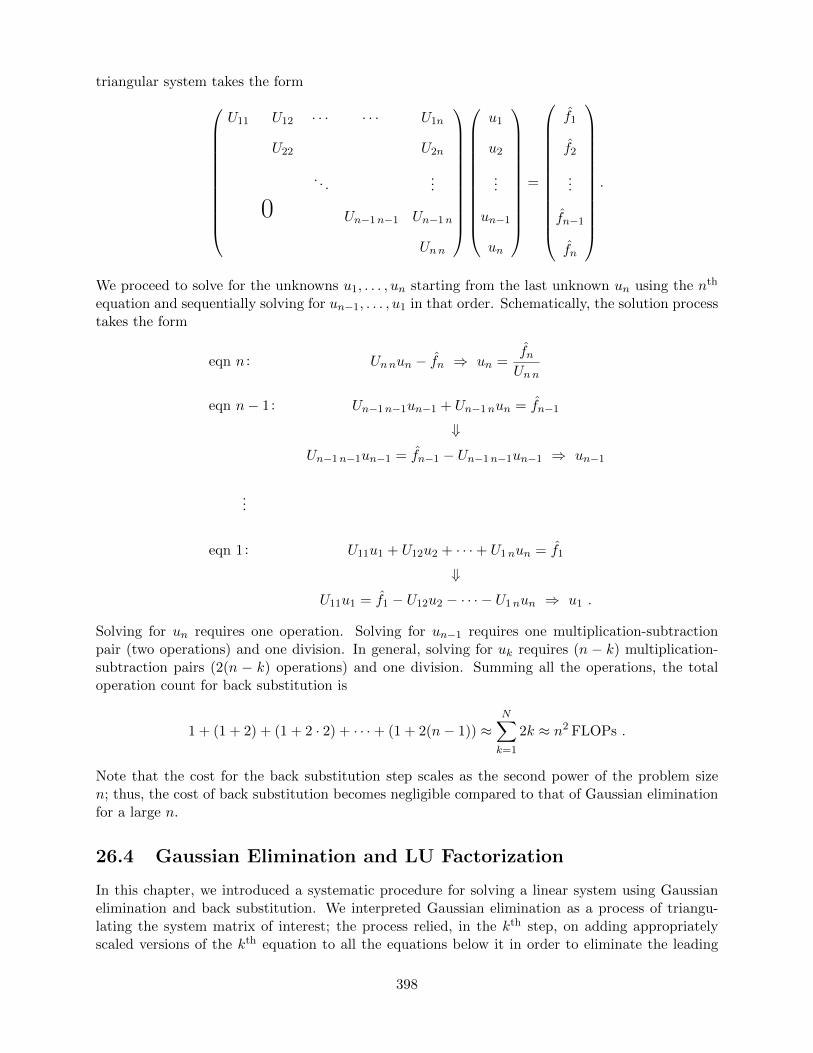
triangular system takes the form

U11 U12 · · · · · · U1n

U22 U2n

. . ....

0 Un−1n−1 Un−1n

Unn

u1

u2

...

un−1

un

=

f1

f2

...

fn−1

fn

.

We proceed to solve for the unknowns u1, . . . , un starting from the last unknown un using the nth

equation and sequentially solving for un−1, . . . , u1 in that order. Schematically, the solution processtakes the form

eqn n : Unnun − fn ⇒ un =fnUnn

eqn n− 1: Un−1n−1un−1 + Un−1nun = fn−1

⇓Un−1n−1un−1 = fn−1 − Un−1n−1un−1 ⇒ un−1

...

eqn 1: U11u1 + U12u2 + · · ·+ U1nun = f1

⇓U11u1 = f1 − U12u2 − · · · − U1nun ⇒ u1 .

Solving for un requires one operation. Solving for un−1 requires one multiplication-subtractionpair (two operations) and one division. In general, solving for uk requires (n − k) multiplication-subtraction pairs (2(n − k) operations) and one division. Summing all the operations, the totaloperation count for back substitution is

1 + (1 + 2) + (1 + 2 · 2) + · · ·+ (1 + 2(n− 1)) ≈N∑k=1

2k ≈ n2 FLOPs .

Note that the cost for the back substitution step scales as the second power of the problem sizen; thus, the cost of back substitution becomes negligible compared to that of Gaussian eliminationfor a large n.

26.4 Gaussian Elimination and LU Factorization

In this chapter, we introduced a systematic procedure for solving a linear system using Gaussianelimination and back substitution. We interpreted Gaussian elimination as a process of triangu-lating the system matrix of interest; the process relied, in the kth step, on adding appropriatelyscaled versions of the kth equation to all the equations below it in order to eliminate the leading

398

coefficient. In particular, we also modified the right-hand side of the equation in the triangulationprocedure such that we are adding the same quantity to both sides of the equation and hence notaffecting the solution. The end product of our triangulation process is an upper triangular matrixU and a modified right-hand side f . If we are given a new right-hand side, we would have to repeatthe same procedure again (in O(n3) cost) to deduce the appropriate new modified right-hand side.

It turns out that a slight modification of our Gaussian elimination procedure in fact wouldpermit solution to the problem with a different right-hand side in O(n2) operations. To achievethis, instead of modifying the right-hand side in the upper triangulation process, we record theoperations used in the upper triangulation process with which we generated the right-hand side. Itturns out that this recording operation in fact can be done using a lower triangular matrix L, suchthat the modified right-hand side f is the solution to

Lf = f, (26.3)

where f is the original right-hand side. Similar to back substitution for an upper triangular system,forward substitution enables solution to the lower triangular system in O(n2) operations. This lowertriangular matrix L that records all operations used in transforming matrix A into U in fact is amatrix that satisfies

A = LU .

In other words, the matrices L and U arise from a factorization of the matrix A into lower andupper triangular matrices.

This procedure is called LU factorization. (The fact that L and U must permit such a factor-ization is straightforward to see from the fact that Uu = f and Lf = f ; multiplication of bothsides of Uu = f by L yields LUu = Lf = f , and because the relationship must hold for anysolution-right-hand-side pair {u, f} to Au = f , it must be that LU = A.) The factorization processis in fact identical to our Gaussian elimination and requires 2n3/3 operations. Note we did computeall the pieces of the matrix L in our elimination procedure; we simply did not form the matrix forsimplicity.

In general the LU decomposition will exist if the matrix A is non-singular. There is, however,one twist: we may need to permute the rows of A — a process known as (partial) pivoting — inorder to avoid a zero pivot which would prematurely terminate the process. (In fact, permutationsof rows can also be advantageous to avoid small pivots which can lead to amplification of round-offerrors.) If even — say in infinite precision — with row permutations we arrive at an exactly zeropivot then this is in fact demonstrates that A is singular.1

There are some matrices for which no pivoting is required. One such important example inmechanical engineering is SPD matrices. For an SPD matrix (which is certainly non-singular — alleigenvalues are positive) we will never arrive at a zero pivot nor we will need to permute rows toensure stability. Note, however, that we may still wish to permute rows to improve the efficiencyof the LU decomposition for sparse systems — which is the topic of the next section.

26.5 Tridiagonal Systems

While the cost of Gaussian elimination scales as n3 for a general n × n linear system, there areinstances in which the scaling is much weaker and hence the computational cost for a large problem

1The latter is a more practical test for singularity of A than say the determinant of A or the eigenvalues of A,however typically singularity of “mechanical engineering” A matrices are not due to devious cancellations but ratherdue to upfront modeling errors — which are best noted and corrected prior to LU decomposition.

399

is relatively low. A tridiagonal system is one such example. A tridigonal system is characterized byhaving nonzero entries only along the main diagonal and the immediate upper and lower diagonal,i.e.

A =

x x

x x x

x x x

x x x

x x x

x x x

x x x

x x

main + 1 diagonal

main diagonalmain − 1 diagonal.

The immediate upper diagonal is called the super-diagonal and the immediate lower diagonal iscalled the sub-diagonal. A significant reduction in the computational cost is achieved by takingadvantage of the sparsity of the tridiagonal matrix. That is, we omit addition and multiplicationof a large number of zeros present in the matrix.

Let us apply Gaussian elimination to the n×n tridiagonal matrix. In the first step, we computethe scaling factor (one FLOP), scale the second entry of the coefficient of the first row by the scalingfactor (one FLOP), and add that to the second coefficient of the second row (one FLOP). (Notethat we do not need to scale and add the first coefficient of the first equation to that of the secondequation because we know it will vanish by construction.) We do not have to add the first equationto any other equations because the first coefficient of all other equations are zero. Moreover, notethat the addition of the (scaled) first row to the second row does not introduce any new nonzeroentry in the second row. Thus, the updated matrix has zeros above the super-diagonal and retainsthe tridiagonal structure of the original matrix (with the (2,1) entry eliminated, of course); inparticular, the updated (n− 1)× (n− 1) sub-block is again tridiagonal. We also modify the right-hand side by multiplying the first entry by the scaling factor (one FLOP) and adding it to thesecond entry (one FLOP). Combined with the three FLOPs required for the matrix manipulation,the total cost for the first step is five FLOPs.

Similarly, in the second step, we use the second equation to eliminate the leading nonzero coef-ficient of the third equation. Because the structure of the problem is identical to the first one, thisalso requires five FLOPs. The updated matrix retain the tridiagonal structure in this eliminationstep and, in particular, the updated (n − 2) × (n − 2) sub-block is tridiagonal. Repeating theoperation for n steps, the total cost for producing an upper triangular system (and the associatedmodified right-hand side) is 5nFLOPs. Note that the cost of Gaussian elimination for a tridiag-onal system scales linearly with the problem size n: a dramatic improvement compared to O(n3)operations required for a general case.

400

At this point, we have produced an upper triangular system of the form

x x

x x 0x x

x x

x x

0 x x

x x

x

u13 FLOPs

u2

...

un−23 FLOPs

un−13 FLOPs

un1 FLOP

=

f1

f1

...

fn−2

fn−1

fn

.

The system is said to be bidiagonal — or more precisely upper bidiagonal — as nonzero entriesappear only on the main diagonal and the super-diagonal. (A matrix that has nonzero entriesonly on the main and sub-diagonal are also said to be bidiagonal; in this case, it would be lowerbidiagonal.)

In the back substitution stage, we can again take advantage of the sparsity — in particularthe bidiagonal structure — of our upper triangular system. As before, evaluation of un requires asimple division (one FLOP). The evaluation of un−1 requires one scaled subtraction of un from theright-hand side (two FLOPs) and one division (one FLOP) for three total FLOPs. The structureis the same for the remaining n−2 unknowns; the evaluating each entry takes three FLOPs. Thus,the total cost of back substitution for a bidiagonal matrix is 3n FLOPs. Combined with the costof the Gaussian elimination for the tridiagonal matrix, the overall cost for solving a tridiagonalsystem is 8n FLOPs. Thus, the operation count of the entire linear solution procedure (Gaussianelimination and back substitution) scales linearly with the problem size for tridiagonal matrices.

We have achieved a significant reduction in computational cost for a tridiagonal system com-pared to a general case by taking advantage of the sparsity structure. In particular, the com-putational cost has been reduced from 2n3/3 to 8n. For example, if we wish to solve for theequilibrium displacement of a n = 1000 spring-mass system (which yields a tridiagonal system),we have reduced the number of operations from an order of a billion to a thousand. In fact, withthe tridiagonal-matrix algorithm that takes advantage of the sparsity pattern, we can easily solvea spring-mass system with millions of unknowns on a desktop machine; this would certainly not bethe case if the general Gaussian elimination algorithm is employed, which would require O(1018)operations.

While many problems in engineering require solution of a linear system with millions (or evenbillions) of unknowns, these systems are typically sparse. (While these systems are rarely tridiag-onal, most of the entries of these matrices are zero nevertheless.) In the next chapter, we considersolution to more general sparse linear systems; just as we observed in this tridiagonal case, the keyto reducing the computational cost for large sparse matrices — and hence making the computationtractable — is to study the nonzero pattern of the sparse matrix and design an algorithm that doesnot execute unnecessary operations.

401

402

Chapter 27

Gaussian Elimination: SparseMatrices

In the previous chapter, we observed that the number of floating point operations required tosolve a n × n tridiagonal system scales as O(n) whereas that for a general (dense) n × n systemscales as O(n3). We achieved this significant reduction in operation count by taking advantage ofthe sparsity of the matrix. In this chapter, we will consider solution of more general sparse linearsystems.

27.1 Banded Matrices

A class of sparse matrices that often arise in engineering practice — especially in continuum me-chanics — is the banded matrix. An example of banded matrix is shown in Figure 27.1. As thefigure shows, the nonzero entries of a banded matrix is confined to within mb entries of the maindiagonal. More precisely,

Aij = 0, for j > i+mb or j < i−mb,

and A may take on any value within the band (including zero). The variable mb is referred to asthe bandwidth. Note that the number of nonzero entries in a n×n banded matrix with a bandwidthmb is less than n(2mb + 1).

Let us consider a few different types of banded matrices.

An×n

un×1

= fn×1

, A =

0

0

mb

mb

Figure 27.1: A banded matrix with bandwidth mb.

403

DRAFT V2.1 © The Authors. License: Creative Commons BY-NC-SA 3.0.

kk == 11

wall

uu33

mm

uu44

mm

uunn

mmnn

uu22

mm22

kk == 11 kk == 11 kk == 11 kk == 11 kk == 11 kk == 11

uu11

mm11

ff11 == 11 ff22 == 11 ff33 == 11 ff44 == 11 ffnn == 11

kk == 11

kk == 11

kk == 11

kk == 11 kk == 11

Figure 27.2: A spring-mass system whose equilibrium state calculation gives rise to a pentadiagonalmatrix.

Example 27.1.1 Tridiagonal matrix: mb = 1As we have discussed in the previous two chapters, tridiagonal matrices have nonzero entries onlyalong the main diagonal, sub-diagonal, and super-diagonal. Pictorially, a tridiagonal matrix takesthe following form:

main diagonal, main ±1 diagonals0

0.

Clearly the bandwidth of a tridiagonal matrix is mb = 1. A n × n tridiagonal matrix arise from,for example, computing the equilibrium displacement of n masses connected by springs, as we haveseen in previous chapters.

·

Example 27.1.2 Pentadiagonal matrix: mb = 2As the name suggests, a pentadiagonal matrix is characterized by having nonzero entries along themain diagonal and the two diagonals above and below it, for the total of five diagonals. Pictorially,a pentadigonal matrix takes the following form:

main diagonal, main ±1, ±2 diagonals0

0.

The bandwidth of a pentadiagonal matrix is mb = 2. A n × n pentadiagonal matrix arise from,for example, computing the equilibrium displacement of n masses each of which is connected tonot only the immediate neighbor but also to the neighbor of the neighbors. An example of such asystem is shown in Figure 27.2.

·

Example 27.1.3 “Outrigger” matrixAnother important type of banded matrix is a matrix whose zero entries are confined to within themb band of the main diagonal but for which a large number of entries between the main diagonaland the most outer band is zero. We will refer to such a matrix as “outrigger.” An example ofsuch a matrix is

“outrigger”

0

0

0

0

mb

.

404

In this example, there are five nonzero diagonal bands, but the two outer bands are located farfrom the middle three bands. The bandwidth of the matrix, mb, is specified by the location ofthe outer diagonals. (Note that this is not a pentadiagonal matrix since the nonzero entries arenot confined to within mb = 2.) “Outrigger” matrices often arise from finite difference (or finiteelement) discretization of partial differential equations in two or higher dimensions.

·

27.2 Matrix-Vector Multiplications

To introduce the concept of sparse operations, let us first consider multiplication of a n× n sparsematrix with a (dense) n-vector. Recall that matrix-vector multiplication may be interpreted row-wise or column-wise. In row-wise interpretation, we consider the task of computing w = Av asperforming n inner products, one for each entry of w, i.e.

wi =(Ai1 Ai2 . . . Ain

)

v1

v2...vn

, i = 1, . . . , n.

If the matrix A is dense, the n inner products of n-vectors requires n ·(2n) = 2n2 FLOPs. However,if the matrix A is sparse, then each row of A contains few nonzero entries; thus, we may skip a largenumber of trivial multiplications in our inner products. In particular, the operation count for theinner product of a sparse n-vector with a dense n-vector is equal to twice the number of nonzeroentries in the sparse vector. Thus, the operation count for the entire matrix-vector multiplicationis equal to twice the number of nonzero entries in the matrix, i.e. 2 · nnz(A), where nnz(A) is thenumber of nonzero entries in A. This agrees with our intuition because the matrix-vector productrequires simply visiting each nonzero entry of A, identifying the appropriate multiplier in v basedon the column index, and adding the product to the appropriate entry of w based on the row index.

Now let us consider a column interpretation of matrix-vector multiplication. In this case, weinterpret w = Av as

w1

w2...wn

= v1

A11

A21...

An1

+ v2

A12

A22...

An2

+ · · ·+ vn

A1n

A2n...

Ann

.

If A is sparse then, each column of A contains few nonzero entries. Thus, for each column we simplyneed to scale these few nonzero entries by the appropriate entry of v and augment the correspondingentries of w; the operation count is twice the number of nonzero entries in the column. Repeatingthe operation for all columns of A, the operation count for the entire matrix-vector multiplicationis again 2 · nnz(A).

Because the number of nonzero entries in a sparse matrix is (by definition) O(n), the operationcount for sparse matrix-vector product is 2 · nnz(A) ∼ O(n). For example, for a banded matrixwith a bandwidth mb, the operation count is at most 2n(2mb + 1). Thus, we achieve a significantreduction in the operation count compared to dense matrix-vector multiplication, which requires2n2 operations.

405

27.3 Gaussian Elimination and Back Substitution

27.3.1 Gaussian Elimination

We now consider the operation count associated with solving a sparse linear system Au = f usingGaussian elimination and back substitution introduced in the previous chapter. Recall that theGaussian elimination is a process of turning a linear system into an upper triangular system, i.e.

step 1: Au = f → U(n×n)upper

triangular

u = f .

For a n× n dense matrix, Gaussian elimination requires approximately 23n

3 FLOPs.

Densely-Populated Banded Systems

Now, let us consider a n× n banded matrix with a bandwidth mb. To analyze the worst case, weassume that all entries within the band are nonzero. In the first step of Gaussian elimination, weidentify the first row as the “pivot row” and eliminate the first entry (column 1) of the first mb

rows by adding appropriately scaled pivot row; column 1 of rows mb + 2, . . . , n are already zero.Elimination of column 1 of a given row requires addition of scaled mb + 1 entries of the pivot row,which requires 2(mb + 1) operations. Applying the operation to mb rows, the operation count forthe first step is approximately 2(mb + 1)2. Note that because the nonzero entries of the pivot rowis confined to the first mb + 1 entries, addition of the scaled pivot row to the first mb + 1 rows doesnot increase the bandwidth of the system (since these rows already have nonzero entries in thesecolumns). In particular, the sparsity pattern of the upper part of A is unaltered in the process.

The second step of Gaussian elimination may be interpreted as applying the first step of Gaus-sian elimination to (n− 1)× (n− 1) submatrix, which itself is a banded matrix with a bandwidthmb (as the first step does not alter the bandwidth of the matrix). Thus, the second eliminationstep also requires approximately 2(mb +1)2 FLOPs. Repeating the operation for all n pivots of thematrix, the total operation count for Gaussian elimination is approximately 2n(mb + 1)2 ∼ O(n).The final upper triangular matrix U takes the following form:

0

0

mb

.

The upper triangular matrix has approximately n(mb + 1) ∼ O(n) nonzero entries. Both theoperation count and the number of nonzero in the final upper triangular matrix are O(n), comparedto O(n3) operations and O(n2) entries for a dense system. (We assume here mb is fixed independentof n.)

In particular, as discussed in the previous chapter, Gaussian elimination of a tridiagonal matrixyields an upper bidiagonal matrix

U =

0

0

main, main +1 diagonals

,

406

in approximately 5n operations (including the formation of the modified right-hand side f). Simi-larly, Gaussian elimination of a pentadiagonal system results in an upper triangular matrix of theform

U =

0

0

main, main +1, +2 diagonals

,

and requires approximately 14n operations.

“Outrigger” Systems: Fill-Ins

Now let us consider application of Gaussian elimination to an “outrigger” system. First, because an× n “outrigger” system with a bandwidth mb is a special case of a “densely-populated banded”system with a bandwidth mb considered above, we know that the operation count for Gaussianelimination is at most n(mb + 1)2 and the number of nonzero in the upper triangular matrix is atmost n(mb + 1). In addition, due to a large number of zero entries between the outer bands of thematrix, we hope that the operation count and the number of nonzero are less than those for the“densely-populated banded” case. Unfortunately, inspection of the Gaussian elimination procedurereveals that this reduction in the cost and storage is not achieved in general.

The inability to reduce the operation count is due to the introduction of “fill-ins”: the entries ofthe sparse matrix that are originally zero but becomes nonzero in the Gaussian elimination process.The introduction of fill-ins is best described graphically. Figure 27.3 shows a sequence of matricesgenerated through Gaussian elimination of a 25 × 25 outrigger system. In the subsequent figures,we color code entries of partially processed U : the shaded area represents rows or columns of pivotsalready processed; the unshaded area represents the rows and columns of pivots not yet processed;the blue represent initial nonzeros in A which remain nonzeros in U -to-be; and the red are initialzeros of A which become nonzero in U -to-be, i.e. fill-ins.

As Figure 27.3(a) shows, the bandwidth of the original matrix is mb = 5. (The values of theentries are hidden in the figure as they are not important in this discussion of fill-ins.) In the firstelimination step, we first eliminate column 1 of row 2 by adding an appropriately scaled row 1 tothe row. While we succeed in eliminating column 1 of row 2, note that we introduce a nonzeroelement in column 6 of row 2 as column 6 of row 1 “falls” to row 2 in the elimination process. Thisnonzero element is called a “fill-in.” Similarly, in eliminating column 1 of row 6, we introduce a“fill-in” in column 2 as column 2 of row 1 “falls” to row 6 in the elimination process. Thus, we haveintroduced two fill-ins in this first elimination step as shown in Figure 27.3(b): one in the upperpart and another in the lower part.

Now, consider the second step of elimination starting from Figure 27.3(b). We first eliminatecolumn 2 of row 3 by adding appropriately scaled row 2 to row 3. This time, we introduce fill innot only from column 7 of row 2 “falling” to row 3, but also from column 6 of row 2 “falling” torow 3. Note that the latter is in fact a fill-in introduced in the first step. In general, once a fill-inis introduced in the upper part, the fill-in propagates from one step to the next, introducing furtherfill-ins as it “falls” through. Next, we need to eliminate column 2 of row 6; this entry was zero inthe original matrix but was filled in the first elimination step. Thus, fill-in introduced in the lowerpart increases the number of rows whose leading entry must be eliminated in the upper-triangulationprocess. The matrix after the second step is shown in Figure 27.3(c). Note that the number offill-in continue to increase, and we begin to lose the zero entries between the outer bands of theoutrigger system.

As shown in Figure 27.3(e), by the beginning of the fifth elimination step, the “outrigger”

407

(a) original system A (b) beginning of step 2, U(k = 1) (c) beginning of step 3, U(k = 2)

(d) beginning of step 4, U(k = 3) (e) beginning of step 5, U(k = 4) (f) beginning of step 15, U(k = 14)

Figure 27.3: Illustration of Gaussian elimination applied to a 25×25 “outrigger” system. The blueentries are the entries present in the original system, and the red entries are “fill-in” introduced inthe factorization process. The pivot for each step is marked by a red square.

408

system has largely lost its sparse structure in the leading (mb + 1) × (mb + 1) subblock of theworking submatrix. Thus, for the subsequent n − mb steps of Gaussian elimination, each steptakes 2m2

b FLOPs, which is approximately the same number of operations as the densely-populatedbanded case. Thus, the total number of operations required for Gaussian elimination of an outriggersystem is approximately 2n(mb + 1)2, the same as the densely-populated banded case. The finalmatrix takes the form:

0

0

mb

upper triangular

inside band (of A): “fill-in”

outside band (of A)no “fill-in”: A, U zero

Note that the number of nonzero entries is approximately n(mb + 1), which is much larger thanthe number of nonzero entries in the original “outrigger” system.

The “outrigger” system, such as the one considered above, naturally arise when a partial differ-ential equation (PDE) is discretized in two or higher dimensions using a finite difference or finiteelement formulation. An example of such a PDE is the heat equation, describing, for example, theequilibrium temperature of a thermal system shown in Figure 27.4. With a natural ordering ofthe degrees of freedom of the discretized system, the bandwidth mb is equal to the number of gridpoints in one coordinate direction, and the number of degrees of freedom of the linear system isn = m2

b (i.e. product of the number of grid points in two coordinate directions). In other words, thebandwidth is the square root of the matrix size, i.e. mb = n1/2. Due to the outrigger structure ofthe resulting system, factorizing the system requires approximately n(mb + 1)2 ≈ n2 FLOPs. Thisis in contrast to one-dimensional case, which yields a tridiagonal system, which can be solved inO(n) operations. In fact, in three dimensions, the bandwidth is equal to the product of the numberof grid points in two coordinate directions, i.e. mb = (n1/3)2 = n2/3. The number of operationsrequired for factorization is n(mb + 1)2 ≈ n7/3. Thus, the cost of solving a PDE is significantlyhigher in three dimensions than in one dimension even if both discretized systems had the samenumber of unknowns.1

27.3.2 Back Substitution

Having analyzed the operation count for Gaussian elimination, let us inspect the operation countfor back substitution. First, recall that back substitution is a process of finding the solution of anupper triangular system, i.e.

step 2: Uu = f → u .

Furthermore, recall that the operation count for back substitution is equal to twice the numberof nonzero entries in U . Because the matrix U is unaltered, we can simply count the number of

1Not unknowns per dimension, but the total number of unknowns.

409

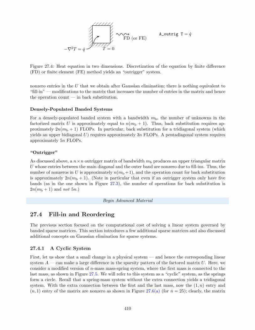
−∇2T = q T = 0

FD (or FE)A_outrig T = q

Figure 27.4: Heat equation in two dimensions. Discretization of the equation by finite difference(FD) or finite element (FE) method yields an “outrigger” system.

nonzero entries in the U that we obtain after Gaussian elimination; there is nothing equivalent to“fill-in” — modifications to the matrix that increases the number of entries in the matrix and hencethe operation count — in back substitution.

Densely-Populated Banded Systems

For a densely-populated banded system with a bandwidth mb, the number of unknowns in thefactorized matrix U is approximately equal to n(mb + 1). Thus, back substitution requires ap-proximately 2n(mb + 1) FLOPs. In particular, back substitution for a tridiagonal system (whichyields an upper bidiagonal U) requires approximately 3n FLOPs. A pentadiagonal system requiresapproximately 5n FLOPs.

“Outrigger”

As discussed above, a n×n outrigger matrix of bandwidth mb produces an upper triangular matrixU whose entries between the main diagonal and the outer band are nonzero due to fill-ins. Thus, thenumber of nonzeros in U is approximately n(mb +1), and the operation count for back substitutionis approximately 2n(mb + 1). (Note in particular that even if an outrigger system only have fivebands (as in the one shown in Figure 27.3), the number of operations for back substitution is2n(mb + 1) and not 5n.)

Begin Advanced Material

27.4 Fill-in and Reordering

The previous section focused on the computational cost of solving a linear system governed bybanded sparse matrices. This section introduces a few additional sparse matrices and also discussedadditional concepts on Gaussian elimination for sparse systems.

27.4.1 A Cyclic System

First, let us show that a small change in a physical system — and hence the corresponding linearsystem A — can make a large difference in the sparsity pattern of the factored matrix U . Here, weconsider a modified version of n-mass mass-spring system, where the first mass is connected to thelast mass, as shown in Figure 27.5. We will refer to this system as a “cyclic” system, as the springsform a circle. Recall that a spring-mass system without the extra connection yields a tridiagonalsystem. With the extra connection between the first and the last mass, now the (1, n) entry and(n, 1) entry of the matrix are nonzero as shown in Figure 27.6(a) (for n = 25); clearly, the matrix

410

wall

ff33

uu33

mm

ff44

uu44

mm

ff55

uu55

mm

ff66

uu66

mm

ff11

uu11

ff22

uu22

mm22

kk == 11 kk == 11 kk == 11 kk == 11 kk == 11 kk == 11

kk == 11

mm11

Figure 27.5: “Cyclic” spring-mass system with n = 6 masses.

(a) original matrix A (b) beginning of step 5 (c) final matrix U

Figure 27.6: Illustration of Gaussian elimination applied to a 25 × 25 “arrow” system. The redentries are “fill-in” introduced in the factorization process. The pivot for each step is marked by ared square.

is no longer tridiagonal. In fact, if apply our standard classification for banded matrices, the cyclicmatrix would be characterized by its bandwidth of mb = n− 1.

Applying Gaussian elimination to the “cyclic” system, we immediately recognize that the(1, n) entry of the original matrix “falls” along the last column, creating n − 2 fill-ins (see Fig-ures 27.6(b) and 27.6(c)). In addition, the original (n, 1) entry also creates a nonzero entry onthe bottom row, which moves across the matrix with the pivot as the matrix is factorized. As aresult, the operation count for the factorization of the “cyclic” system is in fact similar to that ofa pentadiagonal system: approximately 14n FLOPs. Applying back substitution to the factoredmatrix — which contains approximately 3n nonzeros — require 5n FLOPs. Thus, solution of thecyclic system — which has just two more nonzero entries than the tridiagonal system — requiresmore than twice the operations (19n vs. 8n). However, it is also important to note that this O(n)operation count is a significant improvement compared to the O(n(mb + 1)2) = O(n3) operationestimate based on classifying the system as a standard “outrigger” with a bandwidth mb = n− 1.

We note that the fill-in structure of U takes the form of a skyline defined by the envelope ofthe columns of the original matrix A. This is a general principal.

27.4.2 Reordering

In constructing a linear system corresponding to our spring-mass system, we associated the jth entryof the solution vector — and hence the jth column of the matrix — with the displacement of the jth

mass (counting from the wall) and associated the ith equation with the force equilibrium condition

411

(a) A (natural, nnz(A) = 460) (b) U (natural, nnz(U) = 1009)

(c) A′ (AMD, nnz(A′) = 460) (d) U ′ (AMD, nnz(U ′) = 657)

Figure 27.7: Comparison of the sparsity pattern and Gaussian elimination fill-ins for a n = 100“outrigger” system resulting from natural ordering and an equivalent system using the approximateminimum degree (AMD) ordering.

of the ith mass. While this is arguably the most “natural” ordering for the spring-mass system,we could have associated a given column and row of the matrix with a different displacementand force equilibrium condition, respectively. Note that this “reordering” of the unknowns andequations of the linear system is equivalent to “swapping” the rows of columns of the matrix, whichis formally known as permutation. Importantly, we can describe the same physical system usingmany different orderings of the unknowns and equations; even if the matrices appear different, thesematrices describing the same physical system may be considered equivalent, as they all produce thesame solution for a given right-hand side (given both the solution and right-hand side are reorderedin a consistent manner).

Reordering can make a significant difference in the number of fill-ins and the operation count.Figure 27.7 shows a comparison of number of fill-ins for an n = 100 linear system arising from twodifferent orderings of a finite different discretization of two-dimensional heat equation on a 10× 10computational grid. An “outrigger” matrix of bandwidth mb = 10 arising from “natural” orderingis shown in Figure 27.7(a). The matrix has 460 nonzero entries. As discussed in the previoussection, Gaussian elimination of the matrix yields an upper triangular matrix U with approximately

412

n(mb + 1) = 1100 nonzero entries (more precisely 1009 for this particular case), which is shownin Figure 27.7(b). An equivalent system obtained using the approximate minimum degree (AMD)ordering is shown in Figure 27.7(c). This newly reordered matrix A′ also has 460 nonzero entriesbecause permuting (or swapping) rows and columns clearly does not change the number of nonzeros.On the other hand, application of Gaussian elimination to this reordered matrix yields an uppertriangular matrix U shown in Figure 27.7(d), which has only 657 nonzero entries. Note that thenumber of fill-in has been reduced by roughly a factor of two: from 1009 − 280 = 729 for the“natural” ordering to 657 − 280 = 377 for the AMD ordering. (The original matrix A has 280nonzero entries in the upper triangular part.)

In general, using an appropriate ordering can significantly reduced the number of fill-ins andhence the computational cost. In particular, for a sparse matrix arising from n-unknown finitedifference (or finite element) discretization of two-dimensional PDEs, we have noted that “natural”ordering produces an “outrigger” system with mb =

√n; Gaussian elimination of the system yields

an upper triangular matrix with n(mb + 1) ≈ n3/2 nonzero entries. On the other hand, the numberof fill-ins for the same system with an optimal (i.e. minimum fill-in) ordering yields an uppertriangular matrix with O(n log(n)) unknowns. Thus, ordering can have significant impact in boththe operation count and storage for large sparse linear systems.

End Advanced Material

27.5 The Evil Inverse

In solving a linear system Au = f , we advocated a two-step strategy that consists of Gaussianelimination and back substitution, i.e.

Gaussian elimination: Au = f ⇒ Uu = f

Back substitution: Uu = f ⇒ u .

Alternatively, we could find u by explicitly forming the inverse of A, A−1. Recall that if A is non-singular (as indicated by, for example, independent columns), there exists a unique matrix A−1

such that

AA−1 = I and A−1A = I.

The inverse matrix A−1 is relevant to solution systems because, in principle, we could

1. Construct A−1;

2. Evaluate u = A−1f (i.e. matrix-vector product).

Note that the second step follows from the fact that

Au = f

A−1Au = A−1f

Iu = A−1f .

While the procedure is mathematically valid, we warn that a linear system should never be solvedby explicitly forming the inverse.

To motivate why explicitly construction of inverse matrices should be avoided, let us study thesparsity pattern of the inverse matrix for a n-mass spring-mass system, an example of which forn = 5 is shown in Figure 27.8. We use the column interpretation of the matrix and associate thecolumn j of A−1 with a vector pj , i.e.

413

wall

ff11 = 00 ff22 = 00 ff33 = 11 ff44 = 00 ff55 = 00

which ?

not in equilibrium

XX

all displacements nonzero

Figure 27.8: Response of a n = 5 spring-mass system to unit loading on mass 3.

A−1 =

p1 p2 p3 . . . pn

1st column of A−1

2nd column of A−1 nth column of A−1

Since Au = f and u = A−1f , we have (using one-handed matrix-vector product),

u = A−1f =

p1 p2 p3 . . . pn

f1

f2

...

fn

= p1f1 + p2f2 + · · ·+ pnfn .

From this expression, it is clear that the vector pj is equal to the displacements of masses due tothe unit force acting on mass j. In particular the ith entry of pj is the displacement of the ith massdue to the unit force on the jth mass.

Now, to deduce nonzero pattern of a vector pj , let us focus on the case shown in Figure 27.8;we will deduce the nonzero entries of p3 for the n = 5 system. Let us consider a sequence of eventsthat takes place when f3 is applied (we focus on qualitative result rather than quantitative result,i.e. whether masses move, not by how much):

1. Mass 3 moves to the right due to the unit load f3.

2. Force exerted by the spring connecting mass 3 and 4 increases as the distance between mass3 and 4 decreases.

3. Mass 4 is no longer in equilibrium as there is a larger force from the left than from the right(i.e. from the spring connecting mass 3 and 4, which is now compressed, than from the springconnecting mass 4 and 5, which is neutral).

414

4. Due to the unbalanced force mass 4 moves to the right.

5. The movement of mass 4 to the left triggers a sequence of event that moves mass 5, just asthe movement of mass 3 displaced mass 4. Namely, the force on the spring connecting mass4 and 5 increases, mass 5 is no longer in equilibrium, and mass 5 moves to the right.

Thus, it is clear that the unit load on mass 3 not only moves mass 3 but also mass 4 and 5 inFigure 27.8. Using the same qualitative argument, we can convince ourselves that mass 1 and 2must also move when mass 3 is displaced by the unit load. Thus, in general, the unit load f3

on mass 3 results in displacing all masses of the system. Recalling that the ith entry of p3 is thedisplacement of the ith mass due to the unit load f3, we conclude that all entries of p3 are nonzero.(In absence of damping, the system excited by the unit load would oscillate and never come to rest;in a real system, intrinsic damping present in the springs brings the system to a new equilibriumstate.)

Generalization of the above argument to a n-mass system is straightforward. Furthermore,using the same argument, we conclude that forcing of any of one of the masses results in displacingall masses. Consequently, for p1, . . . , pn, we have

u[for f = (1 0 · · · 0)T] = p1 ← nonzero in all entries!

u[for f = (0 1 · · · 0)T] = p2 ← nonzero in all entries!

...

u[for f = (0 0 · · · 0)T] = pn ← nonzero in all entries!

Recalling that pj is the jth column of A−1, we conclude that

A−1 =

p1 p2 · · · pn

is full even though (here) A is tridiagonal. In general A−1 does not preserve sparsity of A and isin fact often full. This is unlike the upper triangular matrix resulting from Gaussian elimination,which preserves a large number of zeros (modulo the fill-ins).

Figure 27.9 shows the system matrix and its inverse for the n = 10 spring-mass system. Thecolors represent the value of each entries; for instance, the A matrix has the typical [−1 2 −1]pattern, except for the first and last equations. Note that the inverse matrix is not sparse and isin fact full. In addition, the values of each column of A−1 agrees with our physical intuition aboutthe displacements to a unit load. For example, when a unit load is applied to mass 3, the distancebetween the wall and mass 1 increases by 1 unit, the distance between mass 1 and 2 increasesby 1 unit, and the distance between mass 3 and 2 increases by 1 unit; the distances between theremaining masses are unaltered because there is no external force acting on the remaining systemat equilibrium (because our system is not clamped on the right end). Accumulating displacementsstarting with mass 1, we conclude that mass 1 moves by 1, mass 2 moves by 2 (the sum of theincreased distances between mass 1 and 2 and mass 2 and 3), mass 3 moves by 3, and all theremaining masses move by 3. This is exactly the information contained in the third column of A−1,which reads [1 2 3 3 . . . 3]T.

In concluding the section, let us analyze the operation count for solving a linear system byexplicitly forming the inverse and performing matrix-vector multiplication. We assume that ourn×n matrix A has a bandwidth of mb. First, we construct the inverse matrix one column at a time

415

(a) A (b) A−1

Figure 27.9: Matrix A for the n = 10 spring-mass system and its inverse A−1. The colors representthe value of each entry as specified by the color bar.

by solving for the equilibrium displacements associated with unit load on each mass. To this end, wefirst compute the LU factorization of A and then repeat forward/backward substitution. Recallingthe operation count for a single forward/backward substitution is O(nm2

b), the construction of A−1

requires

Ap1 =

10...0

⇒ p1 O(nm2b) FLOPs

...

Apn =

00...1

⇒ pn O(nm2b) FLOPs

for the total work of n · O(nm2b) ∼ O(n2m2

b) FLOPs. Once we formed the inverse matrix, we cansolve for the displacement by performing (dense) matrix-vector multiplication, i.e.

u1

u2...un

=

x x · · · xx x · · · x...

.... . .

...x x · · · x

f1

f2...fn

O(n · n) = O(n2) FLOPs

A−1 (full) one-handed or two-handed

.

Thus, both the construction of the inverse matrix and the matrix-vector multiplication requireO(n2) operations. In contrast recall that Gaussian elimination and back substitution solves asparse linear system in O(n) operations. Thus, a large sparse linear system should never be solvedby explicitly forming its inverse.

416

Chapter 28

Sparse Matrices in Matlab

Throughout this chapter we shall assume that A is an n × n sparse matrix. By “sparse” herewe mean that most of the entries of A are zero. We shall define the number of nonzero entries of Aby nnz(A). Thus, by our assumption on sparsity, nnz(A) is small compared to n2; in fact, in all ofour examples, and indeed in many MechE examples, nnz(A) is typically cn, for a constant c whichis O(1) — say c = 3, or 4, or 10. (We will often consider families of matrices A in which case wecould state more precisely that c is independent of n.)

28.1 The Matrix Vector Product

To illustrate some of the fundamental aspects of computations with sparse matrices we shall considerthe calculation of the matrix vector product, w = Av, for A a given n× n sparse matrix as definedabove and v a given n × 1 vector. (Note that we considering here the simpler forward problem,in which v is known and w unknown; in a later section we consider the more difficult “inverse”problem, in which w is known and v is unknown.)

28.1.1 A Mental Model

We first consider a mental model which provides intuition as to how the sparse matrix vectorproduct is calculated. We then turn to actual Matlab implementation which is different in detailfrom the mental model but very similar in concept. There are two aspects to sparse matrices: howthese matrices are stored (efficiently); and how these matrices are manipulated (efficiently). Wefirst consider storage.

Storage

By definition our matrix A is mostly zeros and hence it would make no sense to store all the entries.Much better is to just store the nnz(A) nonzero entries with the convention that all other entriesare indeed zero. This can be done by storing the indices of the nonzero entries as well as the values,

417

DRAFT V2.1 © The Authors. License: Creative Commons BY-NC-SA 3.0.

as indicated in (28.1).

I(m), J(m), 1 ≤ m ≤ nnz(A) :

indices i = I(m), j = J(m)

for which Aij 6= 0

VA(m), 1 ≤ m ≤ nnz(A) :

value of AI(m),J(m)

O(nnz(A)) storage

� n2 if sparse. (28.1)

Here m is an index associated to each nonzero entry, I(m), J(m) are the indices of the mth nonzeroentry, and VA(m) is the value of A associated with this index, VA(m) ≡ AI(m),J(m). Note that VAis a vector and not a matrix. It is clear that if A is in fact dense then the scheme (28.1) actuallyrequires more storage than the conventional non-sparse format since we store values of the indicesas well as the values of the matrix; but for sparse matrices the scheme (28.1) can result in significanteconomies.

As a simple example we consider A = I, the n× n identity matrix, for which nnz(A) = n — avery sparse matrix. Here our sparse storage scheme can be depicted as in (28.2).

x

x

x

x

x

x

m = 1

m = n

m

m = 1: I(1) = 1, J(1) = 1 VA(1) = 1

m = 2: I(2) = 2, J(2) = 2 VA(2) = 1

...

m = n : I(n) = 1, J(n) = n VA(n) = 1

O(n) (� n2) .

storage

(28.2)We note that the mapping between the index m and the nonzero entries of A is of course non-unique; in the above we identify m with the row (or equivalently, column) of the entry on the maindiagonal, but we could equally well number backwards or “randomly.”

Operations

We now consider the sparse matrix-vector product in terms of the storage scheme introducedabove. In particular, we claim that

w︸︷︷︸to find

= A v︸︷︷︸given

can be implemented as

w = zeros(n, 1)

for m = 1: nnz(A)

w(I(m)) = w(I(m)) + VA(m)AI(m),J(m)

× v(J(m))

end

We now discuss why this algorithm yields the desired result.

418

We first note that for any i such that I(m) 6= i for any m — in other words, a row i of A which isentirely zero — w(i) should equal zero by the usual row interpretation of the matrix vector product:w(i) is the inner product between the ith row of A — all zeros — and the vector v, which vanishesfor any v.

i→

0 0 · · · 0 0

A

x

x

...

x

v

=

0

w

On the other hand, for any i such that I(m) = i for some m,

w(i) =

n∑j=1

Aijvj =

n∑j = 1Aij 6= 0

Aijvj .

In both cases the sparse procedure yields the correct result and furthermore does not perform allthe unnecessary operations associated with elements Aij which are zero and which will clearly notcontribute to the matrix vector product: zero rows of A are never visited; and in rows of A withnonzero entries only the nonzero columns are visited. We conclude that the operation count isO(nnz(A)) which is much less than n2 if our matrix is indeed sparse.

We note that we have not necessarily used all possible sparsity since in addition to zeros in Athere may also be zeros in v; we may then not only disregard any row of A which are is zero butwe may also disregard any column k of A for which vk = 0. In practice in most MechE examplesthe sparsity in A is much more important to computational efficiency and arises much more oftenin actual practice than the sparsity in v, and hence we shall not consider the latter further.

28.1.2 Matlab Implementation

It is important to recognize that sparse is an attribute associated not just with the matrix A ina linear algebra or mathematical sense but also an attribute in Matlab (or other programminglanguages) which indicates a particular data type or class (or, in Matlab , attribute). In situationsin which confusion might occur we shall typically refer to the former simply as sparse and thelatter as “declared” sparse. In general we will realize the computational savings associated with amathematically sparse matrix A only if the corresponding Matlab entity, A, is also declared sparse— it is the latter that correctly invokes the sparse storage and algorithms described in the previoussection. (We recall here that the Matlab implementation of sparse storage and sparse methods isconceptually similarly to our mental model described above but not identical in terms of details.)

Storage

We proceed by introducing a brief example which illustrates most of the necessary Matlab func-tionality and syntax. In particular, the script

n = 5;

419

K = spalloc(n,n,3*n);

K(1,1) = 2;

K(1,2) = -1;

for i = 2:n-1

K(i,i) = 2;

K(i,i-1) = -1;

K(i,i+1) = -1;

end

K(n,n) = 1;

K(n,n-1) = -1;

is_K_sparse = issparse(K)

K

num_nonzeros_K = nnz(K)

spy(K)

K_full = full(K)

K_sparse_too = sparse(K_full)

yields the output

is_K_sparse =

1

K =

(1,1) 2

(2,1) -1

(1,2) -1

(2,2) 2

(3,2) -1

(2,3) -1

(3,3) 2

(4,3) -1

(3,4) -1

(4,4) 2

(5,4) -1

(4,5) -1

(5,5) 1

num_nonzeros_K =

420

0 1 2 3 4 5 6

0

1

2

3

4

5

6

Figure 28.1: Output of spy(K).

13

K_full =

2 -1 0 0 0

-1 2 -1 0 0

0 -1 2 -1 0

0 0 -1 2 -1

0 0 0 -1 1

K_sparse_too =

(1,1) 2

(2,1) -1

(1,2) -1

(2,2) 2

(3,2) -1

(2,3) -1

(3,3) 2

(4,3) -1

(3,4) -1

(4,4) 2

(5,4) -1

(4,5) -1

(5,5) 1

as well as Figure 28.1.We now explain the different parts in more detail:

First, M = spalloc(n1,n2,k) (i) creates a declared sparse array M of size n1× n2 with allo-cation for k nonzero matrix entries, and then (ii) initializes the array M to all zeros. (If later

421

in the script this allocation may be exceeded there is no failure or error, however efficiencywill suffer as memory will not be as contiguously assigned.) In our case here, we anticipatethat K will be tri-diagonal and hence there will be less than 3*n nonzero entries.

Then we assign the elements of K — we create a simple tri-diagonal matrix associated withn = 5 springs in series. Note that although K is declared sparse we do not need to assignvalues according to any complicated sparse storage scheme: we assign and more generallyrefer to the elements of K with the usual indices, and the sparse storage bookkeeping ishandled by Matlab under the hood.

We can confirm that a matrix M is indeed (declared) sparse with issparse — issparse(M)

returns a logical 1 if M is sparse and a logical 0 if M is not sparse. (In the latter case, we will notsave on memory or operations.) As we discuss below, some Matlab operations may acceptsparse operands but under certain conditions return non-sparse results; it is often importantto confirm with issparse that a matrix which is intended to be sparse is indeed (declared)sparse.

Now we display K. We observe directly the sparse storage format described in the previoussection: Matlab displays effectively (I(m), J(m), VA(m)) triplets (Matlab does not displaym, which as we indicated is in any event an arbitrary label).

The Matlab built-in function nnz(M) returns the number of nonzero entries in a matrix M.The Matlab built-in function spy(M) displays the n1 × n2 matrix M as a rectangular gridwith (only) the nonzero entries displayed as blue filled circles — Figure 28.1 displays spy(K).In short, nnz and spy permit us to quantify the sparsity and structure, respectively, of amatrix M.

The Matlab built-in functions full and sparse create a full matrix from a (declared) sparsematrix and a (declared) sparse matrix from a full matrix respectively. Note however, that itis better to initialize a sparse matrix with spalloc rather than simply create a full matrixand then invoke sparse; the latter will require at least temporarily (but sometimes fatally)much more memory than the former.

There are many other sparse Matlab built-in functions for performing various operations.

Operations

This section is very brief: once a matrix A is declared sparse, then the Matlab statement w = A*v

will invoke the efficient sparse matrix vector product described above. In short, the (matrix) mul-tiplication operator * recognizes that A is a (declared) sparse matrix object and then automaticallyinvokes the correct/efficient “method” of interpretation and evaluation. Note in the most commonapplication and in our case most relevant application the matrix A will be declared sparse, the vec-tor v will be full (i.e., not declared sparse), and the output vector w will be full (i.e., not declaredsparse).1 We emphasize that if the matrix A is mathematically sparse but not declared sparse thenthe Matlab * operand will invoke the standard full matrix-vector multiply and we not realize thepotential computational savings.

1Note if the vector v is also declared sparse then the result w will be declared sparse as well.

422

28.2 Sparse Gaussian Elimination

This section is also very brief. As we already described in Unit III, in order to solve the matrixsystem Au = f in Matlab we need only write u = A \ f — the famous backslash operator. Wecan now reveal, armed with the material from the current unit, that the backslash operator in factperforms Gaussian elimination (except for overdetermined systems, in which case the least-squaresproblem is solved by a QR algorithm). The backslash will automatically perform partial pivoting— permutations of rows to choose the maximum-magnitude available pivot — to ensure for a non-singular matrix K that a zero pivot is never encountered and that furthermore amplification ofnumerical round-off errors (in finite precision) is minimized.

The sparse case is similarly streamlined. If A is a mathematically sparse matrix and we wishto solve Au = f by sparse Gaussian elimination as described in the previous chapter, we need onlymake sure that A is declared sparse and then write u = A \ f . (As for the matrix vector product,f need not be declared sparse and the result u will not be sparse.) In this case the backslashdoes more than simply eliminate unnecessary calculations with zero operands: the backslash willpermute columns (a reordering) in order to minimize fill-in during the elimination procedure. (Asfor the non-sparse case, row permutations will also be pursued, for purposes of numerical stability.)

The case of A SPD is noteworthy. As already indicated, in this case the Gaussian eliminationprocess is numerically stable without any row permutations. For an SPD matrix, the backslashoperator will thus permute the rows in a similar fashion to the columns; the columns, as before, arepermuted to minimize fill-in, as described in the previous chapter. A particular variant of Gaussianelimination, the Cholesky factorization, is pursued in the SPD case.

423

424

Unit VI

Nonlinear Equations

425

Chapter 29

Newton Iteration

29.1 Introduction

The demonstration robot arm of Figure 29.1 is represented schematically in Figure 29.2. Notethat although the robot of Figure 29.1 has three degrees-of-freedom (“shoulder,” “elbow,” and“waist”), we will be dealing with only two degrees-of-freedom — “shoulder” and “elbow” — in thisassignment.

Figure 29.1: Demonstration robot arm.

Figure 29.2: Schematic of robot arm.

The forward kinematics of the robot arm determine the coordinates of the end effector X =

427

(Robot and photograph courtesy of James Penn.)

DRAFT V2.1 © The Authors. License: Creative Commons BY-NC-SA 3.0.

[X1, X2]T for given joint angles Q = [Q1, Q2]T as[X1

X2

](Q) =

[L1 cos(Q1) + L2 cos(Q1 +Q2)

L1 sin(Q1) + L2 sin(Q1 +Q2)

], (29.1)

where L1 and L2 are the lengths of the first and second arm links, respectively. For our robot,L1 = 4 inches and L2 = 3.025 inches.

The inverse kinematics of the robot arm — the joint angles Q needed to realize a particularend effector position X — are not so straightforward and, for many more complex robot arms, aclosed-form solution does not exist. In this assignment, we will solve the inverse kinematic problemfor a two degree-of-freedom, planar robot arm by solving numerically for Q1 and Q2 from the setof nonlinear Equations (29.1) .

Given a trajectory of data vectors X(i), 1 ≤ i ≤ p — a sequence of p desired end effectorpositions — the corresponding joint angles satisfy

F(Q(i),X(i))= 0, 1 ≤ i ≤ p , (29.2)

where

F (q,X) =

[F1

F2

]=

[L1 cos(q1) + L2 cos(q1 + q2)−X1

L1 sin(q1) + L2 sin(q1 + q2)−X2

].

For the robot “home” position, Xhome ≈ [−0.7154, 6.9635]T, the joint angles are known: Qhome =[1.6, 0.17]T (in radians). We shall assume that X(1) = Xhome and hence Q(1) = Qhome in all cases;it will remain to find Q(2), . . . ,Q(p).

Based on the design of our robot, we impose the following physical constraints on Q1 and Q2:

sin(Q1) ≥ 0 ; sin(Q2) ≥ 0 . (29.3)

Note that a mathematically valid solution of Equation (29.2) might not satisfy the constraints ofEquation (29.3) and, therefore, will need to be checked for physical consistency.

Previously we considered solving equations of the form Ax = b for solution X, given appropri-ately sized matrix and vector A and b. In the univariate case with scalar (1× 1) A and b, we couldvisualize the solution of these linear systems of equations as finding the zero crossing (root) of theline f(x) = Ax− b, as shown in Figure 29.3(a).

Now we will consider the solution of nonlinear systems of equations f(z) = 0 for root Z, whereterms such as powers of z, transcendental functions of z, discontinuous functions of z, or any othersuch nonlinearities preclude the linear model. In the univariate case, we can visualize the solutionof the nonlinear system as finding the roots of a nonlinear function, as shown in Figure 29.3(b)for a cubic, f(z). Our robot example of Figures 29.1 and 29.2 represent a bivariate example of anonlinear system (in which F plays the role of f , and Q plays the role of Z — the root we wish tofind).

In general, a linear system of equations may have no solution, one solution (a unique solution), oran infinite family of solutions. In contrast, a nonlinear problem may have no solution, one solution,two solutions, three solutions (as in Figure 29.3(b)), any number of solutions, or an infinite familyof solutions. We will also need to decide which solutions (of a nonlinear problem) are of interest orrelevant given the context and also stability considerations.

The nonlinear problem is typically solved as a sequence of linear problems — hence buildsdirectly on linear algebra. The sequence of linear problems can be generated in a variety of fashions;our focus here is Newton’s method. Many other approaches are also possible — for example, leastsquares/optimization — for solution of nonlinear problems.

The fundamental approach of Newton’s method is simple:

428

−4 −2 0 2 4 6 8 10

−15

−10

−5

0

5

10

15

20

f(x) = 3x − 6 = 0

x

f(x)

(a) linear function

−6 −4 −2 0 2 4−80

−60

−40

−20

0

20

40

60

80f(z) = z3 + 3z2 − 6z − 8 = 0

z

f(z)

(b) nonlinear function

Figure 29.3: Solutions of univariate linear and nonlinear equations.

• Start with an initial guess or approximation for the root of a nonlinear system.

• Linearize the system around that initial approximation and solve the resulting linear systemto find a better approximation for the root.

• Continue linearizing and solving until satisfied with the accuracy of the approximation.

This approach is identical for both univariate (one equation in one variable) and multivariate(n equations in n variables) systems. We will first consider the univariate case and then extend ouranalysis to the multivariate case.

29.2 Univariate Newton

29.2.1 The Method

Given a univariate function f(z), we wish to find a real zero/root Z of f such that f(Z) = 0. Notethat z is any real value (for which the function is defined), whereas Z is a particular value of z atwhich f(z = Z) is zero; in other words, Z is a root of f(z).

We first start with an initial approximation (guess) z0 for the zero Z. We next approximatethe function f(z) with its first-order Taylor series expansion around z0, which is the line tangentto f(z) at z = z0

f0linear(z) ≡ f ′(z0)(z − z0) + f(z0) . (29.4)

We find the zero z1 of the linearized system f0linear(z) by

f0linear(z

1) ≡ f ′(z0)(z1 − z0) + f(z0) = 0 , (29.5)

which yields

z1 = z0 − f(z0)

f ′(z0). (29.6)

We then repeat the procedure with z1 to find z2 and so on, finding successively better approxi-mations to the zero of the original system f(z) from our linear approximations fklinear(z) until wereach zN such that |f(zN )| is within some desired tolerance of zero. (To be more rigorous, we mustrelate |f(zN )| to |Z − zN |.)

429

Figure 29.4: Graphical illustration of the Newton root finding method.

29.2.2 An Example

The first few steps of the following example have been illustrated in Figure 29.4.We wish to use the Newton method to find a solution to the equation

z2 + 2z = 3 . (29.7)

We begin by converting the problem to a root-finding problem

f(Z) = Z2 + 2Z − 3 = 0 . (29.8)

We next note that the derivative of f is given by

f ′(z) = 2z + 2 . (29.9)

We start with initial guess z0 = 4. We then linearize around z0 to get

f0linear(z) ≡ f ′(z0)(z − z0) + f(z0) = 10(z − 4) + 21 . (29.10)

We solve the linearized system

f0linear(z

1) ≡ 10(z − 4) + 21 = 0 (29.11)

to find the next approximation for the root of f(z),

z1 = 1.9 . (29.12)

430

We repeat the procedure to find

f1linear(z) ≡ f ′(z1)(z − z1) + f(z1) = 5.8(z − 1.9) + 4.41 (29.13)

f1linear(z

2) = 0 (29.14)

z2 = 1.1397 ; (29.15)

f2linear(z) ≡ f ′(z2)(z − z2) + f(z2) = 4.2793(z − 1.1397) + 0.5781 (29.16)

f2linear(z

3) = 0 (29.17)

z3 = 1.0046 . (29.18)

Note the rapid convergence to the actual root Z = 1. Within three iterations the error has beenreduced to 0.15% of its original value.

29.2.3 The Algorithm

The algorithm for the univariate Newton’s method is a simple while loop. If we wish to store theintermediate approximations for the zero, the algorithm is shown in Algorithm 1. If we don’t needto save the intermediate approximations, the algorithm is shown in Algorithm 2.

If, for some reason, we cannot compute the derivative f ′(zk) directly, we can substitute thefinite difference approximation of the derivative (see Chapter 3) for some arbitrary (small) given∆z, which, for the backward difference is given by

f ′(zk) ≈ f(zk)− f(zk −∆z)

∆z. (29.19)

In practice, for ∆z sufficiently small (but not too small — round-off), Newton with approximatederivative will behave similarly to Newton with exact derivative.

Algorithm 1 Newton algorithm with storage of intermediate approximations

k ← 0while

∣∣∣f(zk)∣∣∣ > tol do

zk+1 ← zk − f(zk)f ′(zk)

k ← k + 1end whileZ ← zk

Algorithm 2 Newton algorithm without storage

z ← z0

while∣∣f(z)

∣∣ > tol do

δz ← −f(z)f ′(z)

z ← z + δzend whileZ ← z

There also exists a method, based on Newton iteration, that directly incorporates a finitedifference approximation of the derivative by using the function values at the two previous iterations

431

(thus requiring two initial guesses) to construct

f ′(zk) ≈ f(zk)− f(zk−1)

zk − zk−1. (29.20)

This is called the secant method because the linear approximation of the function is no longer aline tangent to the function, but a secant line. This method works well with one variable (with amodest reduction in convergence rate); the generalization of the secant method to the multivariatecase (and quasi-Newton methods) is more advanced.

Another root-finding method that works well (although slowly) in the univariate case is thebisection (or “binary chop”) method. The bisection method finds the root within a given intervalby dividing the interval in half on each iteration and keeping only the half whose function evaluationsat its endpoints are of opposite sign — and which, therefore, must contain the root. This method isvery simple and robust — it works even for non-smooth functions — but, because it fails to exploitany information regarding the derivative of the function, it is slow. It also cannot be generalizedto the multivariate case.

29.2.4 Convergence Rate

When Newton works, it works extremely fast. More precisely, if we denote the error in Newton’sapproximation for the root at the kth iteration as

εk = zk − Z, (29.21)

then if

(i) f(z) is smooth (e.g., the second derivative exists),

(ii) f ′(Z) 6= 0 (i.e., the derivative at the root is nonzero), and

(iii)∣∣ε0∣∣ (the error of our initial guess) is sufficiently small,

we can show that we achieve quadratic (i.e., εk+1 ∼ (εk)2) convergence:

εk+1 ∼ (εk)2

(1

2

f ′′(Z)

f ′(Z)

). (29.22)

Each iteration doubles the number of correct digits; this is extremely fast convergence. For ourprevious example, the sequence of approximations obtained is shown in Table 29.1. Note thatthe doubling of correct digits applies only once we have at least one correct digit. For the secantmethod, the convergence rate is slightly slower:

εk+1 ∼ (εk)γ , (29.23)

where γ ≈ 1.618.

Proof. A sketch of the proof for Newton’s convergence rate is shown below:

432

iteration approximation number of correct digits

0 4 0

1 1.9 1

2 1.1... 1

3 1.004... 3

4 1.000005... 6

5 1.000000000006... 12

Table 29.1: Convergence of Newton for the example problem.

zk+1 = zk − f(zk)

f ′(zk)(29.24)

��Z + εk+1 =��Z + εk − f(Z + εk)

f ′(Z + εk)(29.25)

εk+1 = εk −���f(Z) + εkf ′(Z) + 1

2(εk)2f ′′(Z) + · · ·f ′(Z) + εkf ′′(Z) + · · · (29.26)

εk+1 = εk − εk f′(Z) + 1

2εkf ′′(Z) + · · ·

f ′(Z)(1 + εk f′′(Z)f ′(Z) + · · · )

(29.27)

εk+1 = εk − εk���f ′(Z)(1 + 1

2εk f′′(Z)f ′(Z) + · · ·

���f ′(Z)(1 + εk f

′′(Z)f ′(Z) + · · · )

; (29.28)

since 11+ρ ∼ 1− ρ+ · · · for small ρ,

εk+1 = εk − εk(

1 +1

2εkf ′′(Z

f ′(Z)

)(1− εk f

′′(Z)

f ′(Z)

)+ · · · (29.29)

εk+1 = ��εk − ��εk +

1

2(εk)2 f

′′(Z)

f ′(Z)+ · · · (29.30)

εk+1 =1

2

f ′′(Z)

f ′(Z)(εk)2 + · · · . (29.31)

We thus confirm the quadratic convergence.

Note that, if f ′(Z) = 0, we must stop at equation (29.26) to obtain the linear (i.e., εk+1 ∼ εk)convergence rate

εk+1 = εk −12(εk)2f ′′(Z) + · · ·

εkf ′′(Z)(29.32)

εk+1 =1

2εk + · · · . (29.33)

In this case, we gain only a constant number of correct digits after each iteration. The bisectionmethod also displays linear convergence.

433

29.2.5 Newton Pathologies

Although Newton often does work well and very fast, we must always be careful not to excite patho-logical (i.e., atypically bad) behavior through our choice of initial guess or through the nonlinearfunction itself.

For example, we can easily — and, thus, this might be less pathology than generally badbehavior — arrive at an “incorrect” solution with Newton if our initial guess is poor. For instance,in our earlier example of Figure 29.4, say that we are interested in finding a positive root, Z > 0, off(z). If we had chosen an initial guess of z0 = −4 instead of z0 = +4, we would have (deservingly)found the root Z = −3 instead of Z = 1. Although in the univariate case we can often avoid thisbehavior by basing our initial guess on a prior inspection of the function, this approach becomesmore difficult in higher dimensions.

Even more diabolical behavior is possible. If the nonlinear function has a local maximum orminimum, it is often possible to excite oscillatory behavior in Newton through our choice of initialguess. For example, if the linear approximations at two points on the function both return theother point as their solution, Newton will oscillate between the two indefinitely and never convergeto any roots. Similarly, if the first derivative is not well behaved in the vicinity of the root, thenNewton may diverge to infinity.

We will later address these issues (when possible) by continuation and homotopy methods.

29.3 Multivariate Newton

29.3.1 A Model Problem

Now we will apply the Newton method to solve multivariate nonlinear systems of equations. Forexample, we can consider the simple bivariate system of nonlinear equations

f1(z1, z2) = z21 + 2z2

2 − 22 = 0 ,

f2(z1, z2) = 2z21 + z2

2 − 17 = 0 .(29.34)

Note that f1 and f2 are the two paraboloids each with principal axes aligned with the coordinatedirections; we plot f1 and f2 in shown in Figure 29.5. We wish to find a zero Z = (z1 z2)T off(z) = (f1(z1, z2) f2(z1, z2))T such that f(Z) = 0. We can visualize Z as the intersections of theellipses f1 = 0 (the intersection of paraboloid f1 with the zero plane) and f2 = 0 (the intersectionof paraboloid f2 with the zero plane). The four solutions (Z1, Z2) = (±2,±3) are shown as the redcircles in the contour plot of Figure 29.6.

29.3.2 The Method

The Newton method for the multivariate case follows the same approach as for the univariate case:

• Start with an initial approximation z0 of a root to the nonlinear system f(z) = 0.

• Linearize the system at z0 and solve the resulting linear system to derive a better approxi-mation z1.

• Continue linearizing and solving until the norm of f(zN ) is within some desired tolerance ofzero.

However, the multivariate case can be much more challenging computationally.

434

−10−5

05

10

−10

−5

0

5

10−100

0

100

200

300

z1

f1(z1, z2) = z21 +2z22 − 22

z2 −10−5

05

10

−10

−5

0

5

10−100

0

100

200

300

z1

f2(z1, z2) = 2z21 + z22 − 17

z2

Figure 29.5: Elliptic Paraboloids f1 and f2.

z1

z 2

Contour plot of f1 and f2

−10 −5 0 5 10−10

−8

−6

−4

−2

0

2

4

6

8

10

Figure 29.6: Contour plots of f1 and f2 with their intersections of the zero contours (the solutionsto f(z) = 0) shown as red circles.

435

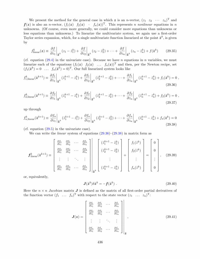
We present the method for the general case in which z is an n-vector, (z1 z2 · · · zn)T andf(z) is also an n-vector, (f1(z) f2(z) · fn(z))T. This represents n nonlinear equations in nunknowns. (Of course, even more generally, we could consider more equations than unknowns orless equations than unknowns.) To linearize the multivariate system, we again use a first-orderTaylor series expansion, which, for a single multivariate function linearized at the point zk, is givenby

fklinear(z) ≡ ∂f

∂z1

∣∣∣∣zk

(z1 − zk1 ) +∂f

∂z2

∣∣∣∣zk

(z2 − zk2 ) + · · ·+ ∂f

∂zn

∣∣∣∣zk

(zn − zkn) + f(zk) (29.35)

(cf. equation (29.4) in the univariate case). Because we have n equations in n variables, we mustlinearize each of the equations (f1(z) f2(z) . . . fn(z))T and then, per the Newton recipe, set(f1(zk) = 0 . . . fn(zk) = 0)T. Our full linearized system looks like

fk1,linear(zk+1) ≡ ∂f1

∂z1

∣∣∣∣zk

(zk+11 − zk1 ) +

∂f1

∂z2

∣∣∣∣zk

(zk+12 − zk2 ) + · · ·+ ∂f1

∂zn

∣∣∣∣zk

(zk+1n − zkn) + f1(zk) = 0 ,

(29.36)

fk2,linear(zk+1) ≡ ∂f2

∂z1

∣∣∣∣zk

(zk+11 − zk1 ) +

∂f2

∂z2

∣∣∣∣zk

(zk+12 − zk2 ) + · · ·+ ∂f2

∂zn

∣∣∣∣zk

(zk+1n − zkn) + f2(zk) = 0 ,

(29.37)

up through

fkn,linear(zk+1) ≡ ∂fn

∂z1

∣∣∣∣zk

(zk+11 − zk1 ) +

∂fn∂z2

∣∣∣∣zk

(zk+12 − zk2 ) + · · ·+ ∂fn

∂zn

∣∣∣∣zk

(zk+1n − zkn) + fn(zk) = 0

(29.38)(cf. equation (29.5) in the univariate case).

We can write the linear system of equations (29.36)–(29.38) in matrix form as

fklinear(zk+1) ≡

∂f1∂z1

∂f1∂z2

· · · ∂f1∂zn

∂f2∂z1

∂f2∂z2

· · · ∂f2∂zn

......

. . ....

∂fn∂z1

∂fn∂z2

· · · ∂fn∂zn

∣∣∣∣∣∣∣∣∣∣∣∣∣∣∣∣zk

(zk+11 − zk1 )

(zk+12 − zk2 )

...

(zk+1n − zkn)

+

f1(zk)

f2(zk)

...

fn(zk)

=

0

0

...

0

, (29.39)

or, equivalently,

J(zk)δzk = −f(zk) . (29.40)

Here the n × n Jacobian matrix J is defined as the matrix of all first-order partial derivatives ofthe function vector (f1 . . . fn)T with respect to the state vector (z1 . . . zn)T:

J(z) =

∂f1∂z1

∂f1∂z2

· · · ∂f1∂zn

∂f2∂z1

∂f2∂z2

· · · ∂f2∂zn

......

. . ....

∂fn∂z1

∂fn∂z2

· · · ∂fn∂zn

∣∣∣∣∣∣∣∣∣∣∣∣∣∣∣∣z

, (29.41)

436

such that the i, jth component of the Jacobian corresponds to the partial derivative of the ith

function with respect to the jth variable,

Jij(z) =∂fi∂zj

(z) . (29.42)

Thus J(zk) denotes the Jacobian matrix for the system evaluated at the point zk. Note also thatδzk is the displacement vector pointing from the current approximation zk to the next approxima-tion zk+1

δzk =

(zk+11 − zk1 )

(zk+12 − zk2 )

...

(zk+1n − zkn)

. (29.43)

Hence δzk is the Newton update to our current iterate.

29.3.3 An Example

We can now apply Newton to solve the n = 2 model problem described in Section 29.3.1:

f1(z1, z2) = z21 + 2z2

2 − 22 = 0 ,

f2(z1, z2) = 2z21 + z2

2 − 17 = 0 .(29.44)

We first compute the elements of the Jacobian matrix as

J11 =∂f1

∂z1= 2z1, J12 =

∂f1

∂z2= 4z2, J21 =

∂f2

∂z1= 4z1, J22 =

∂f2

∂z2= 2z2 , (29.45)

and write the full matrix as

J(z) =

J11 J12

J21 J22

=

2z1 4z2

4z1 2z2

. (29.46)

We can now perform the iteration.We start with initial guess z0 = (10 10)T. We next linearize around z0 to get

f0linear(z) ≡ J(z0)(z − z0) + f(z0) =

20 40

40 20

δz0 +

278

283

. (29.47)

Note that we can visualize this system as two planes tangent to f1 and f2 at z0. We now solve thelinearized system

f0linear(z

1) ≡

20 40

40 20

δz0 +

278

283

=

0

0

(29.48)

or 20 40

40 20

δz0 =

−278

−283

(29.49)

437

to find

δz0 =

−4.8

−4.55

; (29.50)

thus the next approximation for the root of f(z) is given by

z1 = z0 + δz0 =

5.2

5.45

. (29.51)

We repeat the procedure to find

f1linear(z) ≡ J(z1)(z − z1) + f(z1) =

10.4 21.8

20.8 10.9

δz1 +

64.445

66.7825

, (29.52)

f1linear(z

2) = 0 (29.53)

z2 =

2.9846

3.5507

; (29.54)

f2linear(z) =≡ J(z2)(z − z2) + f(z2) =

5.9692 14.2028

11.9385 7.1014

δz2 +

12.1227

13.4232

, (29.55)

f2linear(z

3) = 0 (29.56)

z3 =

2.1624

3.0427

. (29.57)

We see that the solution rapidly approaches the (nearest) exact solution Z = (2 3)T.

29.3.4 The Algorithm

The multivariate Newton algorithm is identical to the univariate algorithm, except that now foreach pass through the while loop we must now solve a linearized system of equations involving theJacobian matrix.

Algorithm 3 Multivariate Newton algorithm without storage

z ← z0

while ‖f(z)‖ > tol do{Solve the linearized system for δz.}J(z)δz = −f(z)z ← z + δz

end whileZ ← z

We can see that the computational cost for the multivariate Newton iteration is essentially thetotal number of iterations multiplied by the cost to solve an n×n linear system — which, if dense,

438

could be as much as O(n3) and, if sparse, as little as O(n) operations. Additionally, for “pure”Newton, the Jacobian needs to be recomputed (O(n2) operations) at each iteration. (In “impure”Newton the Jacobian sometimes is held fixed for several iterations or updated selectively.)

Note that, as before in the univariate case, we can substitute a finite difference approximation forthe Jacobian if we can not (or choose not to) use the analytical expressions. Here we first introducea scalar ∆z (small); note that ∆z is not related to δz — i.e., this is not a secant approach. Thenwe approximate, for 1 ≤ i ≤ n, 1 ≤ j ≤ n,

Jij(z) ≡ ∂fi∂zj

(z) ≈ fi(z + ∆zej)− fi(z)

∆z≡ Jij(z), (29.58)

where ej is the unit vector in the j-direction such that z + ∆zej differs from z in only the jth

component — a partial difference approximation to the partial derivative ∂fi∂zj

. Note that to compute

the full finite difference approximation n× n matrix J(z) we need O(n2) function evaluations.

29.3.5 Comments on Multivariate Newton

For multivariate Newton, both the convergence rate and the pathologies are similar to the univariatecase, although the pathologies are somewhat more likely in the multivariate case given the greaternumber of degrees of freedom.

The main difference for the multivariate case, then, is the relative cost of each Newton itera-tion (worst case O(n3) operations) owing to the size of the linear system which must be solved.For this reason, Newton’s rapid convergence becomes more crucial with growing dimensionality.Thanks to the rapid convergence, Newton often outperforms “simpler” approaches which are lesscomputationally expensive per iteration but require many more iterations to converge to a solution.

29.4 Continuation and Homotopy

Often we are interested not in solving just a single nonlinear problem, but rather a family ofnonlinear problems f(Z;µ) = 0 with real parameter µ which can take on a sequence of valuesµ(1), . . . , µ(p). Typically we supplement f(Z;µ) = 0 with some simple constraints or continuityconditions which select a particular solution from several possible solutions.

We then wish to ensure that, (i) we are able to start out at all, often by transforming theinitial problem for µ = µ(1) (and perhaps also subsequent problems for µ = µ(i)) into a seriesof simpler problems (homotopy) and, (ii) once started, and as the parameter µ is varied, wecontinue to converge to “correct” solutions as defined by our constraints and continuity conditions(continuation).

29.4.1 Parametrized Nonlinear Problems: A Single Parameter

Given f(Z;µ) = 0 with real single parameter µ, we are typically interested in how our solutionZ changes as we change µ; in particular, we now interpret (a la the implicit function theorem) Zas a function Z(µ). We can visualize this dependency by plotting Z (here n = 1) with respect toµ, giving us a bifurcation diagram of the problem, as depicted in Figure 29.7 for several commonmodes of behavior.

Figure 29.7(a) depicts two isolated solution branches with two, distinct real solutions overthe whole range of µ. Figure 29.7(b) depicts two solution branches that converge at a singularpoint , where a change in µ can drive the solution onto either of the two branches. Figure 29.7(c)depicts two solution branches that converge at a limit point , beyond which there is no solution.

439

(a) isolated branches (b) singular point

(c) limit point (d) isola

(e) pitchfork

Figure 29.7: Bifurcation Diagram: Several Common Modes of Behavior.

440

Figure 29.8: Simple mechanical linkage.

Figure 29.7(d) depicts an isola, an isolated interval of two solution branches with two limit pointsfor endpoints. Figure 29.7(e) depicts a single solution branch that “bifurcates” into several solutionsat a pitchfork ; pitchfork bifurcations often correspond to nonlinear dynamics that can display eitherstable (represented by solid lines in the figure) or unstable (represented by dotted lines) behavior,where stability refers to the ability of the state variable Z to return to the solution when perturbed.

Note that, for all of the mentioned cases, when we reach a singular or limit point — characterizedby the convergence of solution branches — the Jacobian becomes singular (non-invertible) and henceNewton breaks down unless supplemented by additional conditions.

29.4.2 A Simple Example

We can develop an intuitive understanding of these different modes of behavior and correspondingbifurcation diagrams by considering a simple example.

We wish to analyze the simple mechanical linkage shown in Figure 29.8 by finding X corre-sponding to an arbitrary θ for given (constant) H, R, and L. In this example, then, θ correspondsto the earlier discussed generic parameter µ.

We can find an analytical solution for X(θ; R, H, L) by solving the geometric constraint

(X − R cos θ)2 + (H − R sin θ)2 = L2 , (29.59)

which defines the distance between the two joints as L. This is clearly a nonlinear equation, owing tothe quadratic term in x. We can eliminate one parameter from the equation by non-dimensionalizingwith respect to L, giving us

(X −R cos θ)2 + (H −R sin θ)2 = 1 , (29.60)

where X = X

L, R = R

L, and H = H

L. Expanding and simplifying, we get

aX2 + bX + c ≡ f(X; θ;R,H) = 0 , (29.61)

where a = 1, b = −2R cos θ, and c = R2 +H2−2HR sin θ−1. A direct application of the quadraticformula then gives us the two roots

X+ =−b+

√b2 − 4ac

2a,

X− =−b−

√b2 − 4ac

2a,

(29.62)

441

which may be real or complex.We observe three categories for the number of solutions to our quadratic equation depending on

the value of the discriminant ∆(θ;R,H) ≡ b2 − 4ac. First, if ∆ < 0,√

∆ is imaginary and there isno (real) solution. An example is the case in which H > L+ R. Second, if ∆ = 0, there is exactlyone solution, X = −b

2a . An example is the case in which H = L + R and θ = π2 . Third, if ∆ > 0,

there are two distinct solutions, X+ and X−; an example is shown in Figure 29.8. Note that withour simple crank example we can obtain all the cases of Figure 29.7 except Figure 29.7(e).

We note that the case of two distinct solutions is new — our linear systems of equations (forthe univariate case, f(x) = Ax − b) had either no solution (A = 0, b 6= 0; line parallel to x axis),exactly one solution (A 6= 0; line intersecting x axis), or an infinite number of solutions (A = 0,b = 0; line on x axis). Nonlinear equations, on the other hand, have no such restrictions. Theycan have no solution, one solution, two solutions (as in our quadratic case above), three solutions(e.g., a cubic equation) — any finite number of solutions, depending on the nature of the particularfunction f(z) — or an infinite number of solutions (e.g., a sinusoidal equation). For example, iff(z) is an nth-order polynomial, there could be anywhere from zero to n (real) solutions, dependingon the values of the n+ 1 parameters of the polynomial.

It is important to note, for the cases in which there are two, distinct solution branches corre-sponding to X+ and X−, that, as we change the θ of the crank, it would be physically impossible tojump from one branch to the other — unless we stopped the mechanism, physically disassembledit, and then reassembled it as a mirror image of itself. Thus for the physically relevant solution wemust require a continuity condition, or equivalently a constraint that requires |X(θ(i))−X(θ(i−1))|not too large or perhaps X(θ(i))X(θ(i−1)) > 0; here θ(i) and θ(i−1) are successive parameters in ourfamily of solutions.

In the Introduction, Section 29.1, we provide an example of a linkage with two degrees offreedom. In this robot arm example the parameter µ is given by X, the desired position of the endeffector.

29.4.3 Path Following: Continuation

As already indicated, as we vary our parameter µ (corresponding to θ in the crank example),we must reflect any constraint (such as, in the crank example, no “re-assembly”) in our numericalapproach to ensure that the solution to which we converge is indeed the “correct” one. One approachis through an appropriate choice of initial guess. Inherent in this imperative is an opportunity— we can exploit information about our previously converged solution not only to keep us onthe appropriate solution branch, but also to assist continued (rapid) convergence of the Newtoniteration.

We denote our previously converged solution to f(Z;µ) = 0 as Z(µ(i−1)) (we consider here

the univariate case). We wish to choose an initial guess Z(µ(i)) to converge to (a nearby root)Z(µ(i)) = Z(µ(i−1) + δµ) for some step δµ in µ. The simplest approach is to use the previouslyconverged solution itself as our initial guess for the next step,

Z(µ(i)) = Z(µ(i−1)) . (29.63)

This is often sufficient for small changes δµ in µ and it is certainly the simplest approach.We can improve our initial guess if we use our knowledge of the rate of change of Z(µ) with

respect to µ to help us extrapolate, to wit

Z(µ(i)) = Z(µ(i−1)) +dZ

dµδµ . (29.64)

442

We can readily calculate dZdµ as

dZ

dµ=−∂f∂µ

∂f∂z

, (29.65)

since

f(Z(µ);µ) = 0⇒ df

dµ(Z(µ);µ) ≡ ∂f

∂z

dZ

dµ+∂f

∂µ �����1

dµ

dµ= 0⇒ dZ

dµ=−∂f∂µ

∂f∂z

, (29.66)

by the chain rule.

29.4.4 Cold Start: Homotopy

In many cases, given a previous solution Z(µ(i−1)), we can use either of equations (29.63) or (29.64)

to arrive at an educated guess Z(µ(i)) for the updated parameter µ(i). If we have no previoussolution, however, (e.g., i = 1) or our continuation techniques fail, we need some other means ofgenerating an initial guess Z(µ(i)) that will be sufficiently good to converge to a correct solution.

A common approach to the “cold start” problem is to transform the original nonlinear prob-lem f(Z(µ(i));µ(i)) = 0 into a form f(Z(µ(i), t);µ(i), t) = 0, i.e., we replace f(Z;µ(i)) = 0 with

f(Z;µ(i), t) = 0. Here t is an additional, artificial , continuation parameter such that, when t = 0,the solution of the nonlinear problem

f(Z(µ(i), t = 0);µ(i), t = 0) = 0 (29.67)

is relatively simple (e.g., linear) or, perhaps, coincides with a preceding, known solution, and, whent = 1,

f(z;µ(i), t = 1) = f(z;µ(i)) (29.68)

such that f(Z(µ(i), t = 1);µ(i), t = 1) = 0 implies f(Z(µ(i));µ(i)) = 0 and hence Z(µ(i)) (the desired

solution) = Z(µ(i), t = 1).We thus transform the “cold start” problem to a continuation problem in the artificial parameter

t as t is varied from 0 to 1 with a start of its own (when t = 0) made significantly less “cold” byits — by construction — relative simplicity, and an end (when t = 1) that brings us smoothly tothe solution of the original “cold start” problem.

As an example, we could replace the crank function f of (29.61) with a function f(X; θ, t;R,H) =at X2 + bX + c such that for t = 0 the problem is linear and the solution readily obtained.

29.4.5 A General Path Approach: Many Parameters

We consider now an n-vector of functions

f(z;µ) = (f1(z;µ) f2(z;µ) . . . fn(z;µ))T (29.69)

that depends on an n-vector of unknowns z

z = (z1 z2 . . . zn)T (29.70)

and a parameter `-vector µ (independent of z)

µ = (µ1 µ2 . . . µ`)T . (29.71)

443

We also introduce an inequality constraint function

C(Z) =

{1 if constraint satisfied

0 if constraint not satisfied. (29.72)

Note this is not a constraint on z but rather a constraint on the (desired) root Z. Then, given µ,we look for Z = (Z1 Z2 . . . Zn)T such that f(Z;µ) = 0

C(Z) = 1. (29.73)

In words, Z is a solution of n nonlinear equations in n unknowns subject which satisfies theconstraint C.

Now we consider a path or “trajectory” — a sequence of p parameter vectors µ(1), . . . , µ(p).We wish to determine Z(i), 1 ≤ i ≤ p, such that f(Z(i);µ(i)) = 0

C(Z(i)) = 1. (29.74)

We assume that Z(1) is known and that Z(2), . . . ,Z(p) remain to be determined. We can expect,then, that as long as consecutive parameter vectors µ(i−1) and µ(i) are sufficiently close, we shouldbe able to use our continuation techniques equations (29.63) or (29.64) to converge to a correct(i.e., satisfying C(Z(i)) = 1) solution Z(i). If, however, µ(i−1) and µ(i) are not sufficiently close,our continuation techniques will not be sufficient (i.e. we will fail to converge to a solution at allor we will fail to converge to a solution satisfying C) and we will need to apply a — we hope —more fail-safe homotopy.

We can thus combine our continuation and homotopy frameworks into a single algorithm. Onesuch approach is summarized in Algorithm 4. The key points of this algorithm are that (i) we areusing the simple continuation approach given by equation (29.63) (i.e., using the previous solutionas the initial guess for the current problem), and (ii) we are using a bisection-type homotopy that,each time Newton fails to converge to a correct solution, inserts a new point in the trajectoryhalfway between the previous correct solution and the failed point. The latter, in the language ofhomotopy, can be expressed as

f(z;µ(i), t) = f(z; (1− t)µ(i−1) + tµ(i)) (29.75)

with t = 0.5 for the inserted point.Although there are numerous other approaches to non-convergence in addition to Algorithm 4,

such as relaxed Newton — in which Newton provides the direction for the update, but then we takejust some small fraction of the proposed step — Algorithm 4 is included mainly for its generality,simplicity, and apparent robustness.

444

Algorithm 4 General Path Following Algorithm

for i = 2: p doZ(i) ← Z(i−1)

repeatZ(i) ← {Solve f(z;µ(i)) = 0 via Newton given initial guess Z(i)}if Newton does not converge OR C(Z(i)) 6= 1 then

for j = p : − 1: i doµ(j+1) ← µ(j) {Shift path parameters by one index to accommodate insertion}

end forµ(i) ← 1

2(µ(i−1) + µ(i)) {Insert point in path halfway between µ(i−1) and µ(i)}p← p+ 1 {Increment p to account for insertion}

end ifuntil Newton converges AND C(Z(i)) = 1

end for

445

MIT OpenCourseWarehttp://ocw.mit.edu

2.086 Numerical Computation for Mechanical EngineersSpring 2013

For information about citing these materials or our Terms of Use, visit: http://ocw.mit.edu/terms.