Math for Eng and Scientists 3
89
Mathematics for Engineers and Scientists 3 F18XC1 Heriot-Watt University
-
Upload
john-wilkinson -
Category
Documents
-
view
77 -
download
8
description
differential equations and multiple integrals application problems,linear approximation and error analysis using Taylor and mclaurin series, partial differential equations, maxima and minima values of differential equation
Transcript of Math for Eng and Scientists 3

Mathematics
for
Engineers and Scientists 3
F18XC1
Heriot-Watt University

2

Contents
1 Introduction to Ordinary Differential Equations 11.1 Terminology . . . . . . . . . . . . . . . . . . . . . . . . . . . . . . . . . . . 21.2 1st Order Differential Equations: Simple Examples . . . . . . . . . . . . . 21.3 1st Order Differential Equation: Separation of Variables . . . . . . . . . . . 31.4 1st Order Differential Equation: Transformations . . . . . . . . . . . . . . 51.5 1st Order Linear Differential Equations: Integrating Factor Method . . . . 6
2 Homogeneous, Linear, Constant-Coefficient, 2nd-Order ODEs 112.1 Introduction to Linear Second-Order Ordinary Differential Equations . . . 112.2 Newton’s second law . . . . . . . . . . . . . . . . . . . . . . . . . . . . . . 122.3 Springs and Hooke’s Law . . . . . . . . . . . . . . . . . . . . . . . . . . . . 132.4 Simple Harmonic Motion . . . . . . . . . . . . . . . . . . . . . . . . . . . . 142.5 Damped oscillations . . . . . . . . . . . . . . . . . . . . . . . . . . . . . . . 162.6 ODE classification (revisited) . . . . . . . . . . . . . . . . . . . . . . . . . 162.7 Homogeneous linear ODEs: The Principle of Superposition . . . . . . . . . 172.8 Solving linear second-order constant-coefficient homogeneous ODEs . . . . 18
2.8.1 Exponential solutions . . . . . . . . . . . . . . . . . . . . . . . . . . 182.8.2 Case I: b2 − 4ac > 0 . . . . . . . . . . . . . . . . . . . . . . . . . . . 182.8.3 Case II: b2 − 4ac = 0 . . . . . . . . . . . . . . . . . . . . . . . . . . 192.8.4 Case III: b2 − 4ac < 0 . . . . . . . . . . . . . . . . . . . . . . . . . . 20
2.9 Practical example: damped springs . . . . . . . . . . . . . . . . . . . . . . 222.9.1 Overdamping: C2 − 4mk > 0 . . . . . . . . . . . . . . . . . . . . . . 232.9.2 Critical damping: C2 − 4mk = 0 . . . . . . . . . . . . . . . . . . . . 242.9.3 Underdamping: C2 − 4mk < 0 . . . . . . . . . . . . . . . . . . . . . 24
3 Inhomogeneous Linear ODEs 273.1 Examples of applications . . . . . . . . . . . . . . . . . . . . . . . . . . . . 273.2 Linear operators . . . . . . . . . . . . . . . . . . . . . . . . . . . . . . . . . 273.3 Solving inhomogeneous linear ODEs . . . . . . . . . . . . . . . . . . . . . . 283.4 Method of undetermined coefficients . . . . . . . . . . . . . . . . . . . . . 293.5 Degenerate inhomogeneities . . . . . . . . . . . . . . . . . . . . . . . . . . 33
4 Partial Differentiation 394.1 Reminder of derivatives of functions of a single variable . . . . . . . . . . . 394.2 Partial derivatives of functions of two variables . . . . . . . . . . . . . . . . 404.3 Higher-order partial derivatives . . . . . . . . . . . . . . . . . . . . . . . . 434.4 Directional Derivatives . . . . . . . . . . . . . . . . . . . . . . . . . . . . . 44
3

4.5 Using the chain rule to find derivatives . . . . . . . . . . . . . . . . . . . . 454.6 Functions of many variables . . . . . . . . . . . . . . . . . . . . . . . . . . 474.7 Partial differential equations . . . . . . . . . . . . . . . . . . . . . . . . . . 48
5 Maxima and Minima 53
6 Taylor Series and Linear Approximation 616.1 Taylor series . . . . . . . . . . . . . . . . . . . . . . . . . . . . . . . . . . . 626.2 Estimation of errors . . . . . . . . . . . . . . . . . . . . . . . . . . . . . . . 63
7 Multiple Integrals 677.1 Integration of functions of one variable . . . . . . . . . . . . . . . . . . . . 677.2 Integration of functions of two variables . . . . . . . . . . . . . . . . . . . . 687.3 Interchanging the order of integration . . . . . . . . . . . . . . . . . . . . . 74
8 Double Integrals: Applications and Polar Coordinates 798.1 Change of variables to polar coordinates . . . . . . . . . . . . . . . . . . . 798.2 Volume . . . . . . . . . . . . . . . . . . . . . . . . . . . . . . . . . . . . . . 818.3 Average values . . . . . . . . . . . . . . . . . . . . . . . . . . . . . . . . . 828.4 Mass and centre of mass . . . . . . . . . . . . . . . . . . . . . . . . . . . . 82
4

Chapter 1
Introduction to Ordinary DifferentialEquations
A differential equation is an equation involving variables (say x and y) and ordinary
derivatives, i.e. dydx, d2y
dx2 .
When the derivative is of the form dydx
then x is the independent variable and y is thedependent variable.
To solve a differential equation of the form dydx
= f(x) means to determine y as a functionof x.
Example 1.1. Find a general solution of the differential equation
dy
dx= 1 .
This can be solved by integrating both sides with respect to x,
∫dy
dxdx =
∫
1 dx, to get
y = x+ A where A is a constant of integration.
Example 1.2. The following differential equation represents how the current I in anelectrical circuit changes with time t,
Ld2I
dt2+R
dI
dt+
1
CI = 0 ,
where L, inductance, R, resistance and C, capacitance are constants.
Here, I is the dependent variable and t is the independent variable (we seek solutions forI in terms of t). Note there is a second derivative d2I
dt2and so this is called a second order
differential equation.
1

1.1 Terminology
The order of a differential equation is determined by the highest order derivative in thedifferential equation.
Example 1.3. The general linear second order differential equation is represented by
a(t)d2y
dt2+ b(t)
dy
dt+ c(t)y = f(t) .
Here, y is the dependent variable and t is the independent variable, the highest orderterm is d2y
dt2and so it is a second order differential equation.
It is linear since the coefficients of y and its derivatives are functions of t only (so thereare no powers of y or its derivatives or products of these). If a differential equation is notlinear it is said to be nonlinear.
If f(t) = 0 the the differential equation is homogeneous. Otherwise it is inhomoge-neous.
1.2 1st Order Differential Equations: Simple Exam-
ples
Example 1.4. Find the general solution of the differential equation
dy
dx= x.
By integrating both sides with respect to x we get the solution
y =1
2x2 + C
where C is an arbitrary constant. As the solution contains an arbitrary constant it iscalled a general solution.
If we are given further information, such as y(0) = 1, we can determine the value of Cand find a particular solution.
Given that y = 1 when x = 0, we have 1 = 0 + C, so that C = 1. Thus, the particularsolution satisfying the condition y(0) = 1 is
y =1
2x2 + 1.
2
Example 1.5. Find the solution of the differential equation
dy
dx= cos x ; y(π/2) = 2.
The general solution isy = sin x+ C
where C is an arbitrary constant.
Given that y = 2 when x = π2, we have 2 = 1+C, so that C = 1. therefore the particular
solution isy = sin x+ 1.
1.3 1st Order Differential Equation: Separation of
Variables
Consider the generic separable differential equation.
dx
dt= f(x)g(t)
This is called separable as the differential equation to be written in the following form
dx
f(x)= g(t) dt
where the functional dependence of x and t are on different sides of the equation. We canthen integrate both sides as follows
∫dx
f(x)=
∫
g(t) dt
to find a general solution to the differential equation.
Example 1.6. Find the solution of the differential equation
dy
dx=
x2
y.
The differential equation can be written in the following form
y dy = x2 dx ⇒∫
y dy =
∫
x2 dx.
3
By performing the integration, the general solution is
1
2y2 =
1
3x3 + C.
Note, we only need one arbitrary constant C.
Example 1.7. Find the solution of the differential equation
dy
dx= y2e−x : y(0) = 0.5.
The differential equation can be written in the following form
1
y2dy = e−x dx ⇒
∫1
y2dy =
∫
e−x dx.
Integrating gives the general solution
−1
y= −e−x + C.
If y = 0.5 when x = 0 we get −2 = −1 + C and so C = −1. The particular solution is
1
y= e−x + 1 ⇒ y =
1
e−x + 1.
Example 1.8. Newton’s second law of motion (‘F = ma’) can be applied to a dragsterthat has deployed its parachute and is slowing down. The differential equation is
F = mdv
dtwhere the drag force F = −1
2CD ρA v2
where CD, the drag coefficient, ρ, the density of air, and A the area of the parachuteare constants. This looks complicated but we can combine all the constants as k =(CDρA)/(2m) to write as a separable differential equation
dv
dt= −kv2.
This can be written as∫
1
v2dy =
∫
−k dt with general solution1
v= kt+ C.
If we are provided with the speed of the dragster when the parachute was deployed, sayv(0) = 30m s−1, we can find a particular solution.
If v = 30 when t = 0 then 1/30 = C. Therefore the particular solution is
1
v= kt+
1
30⇒ 1
v=
30kt+ 1
30⇒ v =
30
30kt+ 1.
4

1.4 1st Order Differential Equation: Transformations
Some differential equations are not separable but can be made separable by using atransformation (or substitution). The first transformation we will consider sets y = vxand considers homogeneous differential equations of the form
dy
dx= f
(y
x
)
.
To apply the transformation we substitute
y = vx anddy
dx= v + x
dv
dx
into the original equations. (Note the substitution for dydx
comes from using the product
rule to give d(vx)dx
= v + xdvdx.) The differential equation is now separable as it can be
written as
v + xdv
dx= f(v) ⇒
∫1
f(v)− vdv =
∫1
xdx
Example 1.9. Find the solution of the differential equation
dy
dx=
y2 + xy
x2which can be writtem as
dy
dx=
(y
x
)2
+(y
x
)
.
Substitute y = vx and dydx
= v + xdvdx
to get
v + xdv
dx=
(vx)2 + x(vx)
x2⇒ v + x
dv
dx= v2 + v ⇒ x
dv
dx= v2.
Using the separable variables methods gives∫
1
v2dv =
∫1
xdx ⇒ −1
v= ln(x) + C.
We substitute v = y/x to return to the original variables
−x
y= ln x+ C ⇒ y =
x
ln x+ C.
Other transformations can be used. For example the transformation v = ax+ by + c canbe used for differential equations of the form
dy
dx= f(ax+ by + c).
To apply the transformation we substitute
v = ax+ by + c anddy
dx=
1
b
(dv
dx− a
)
into the original equations.
5

Example 1.10. Find the solution of the differential equation
dy
dx=
x− y + 2
x− y + 3.
Let v = x− y+3 and therefore substitute y = x− v+3 and dydx
= 1− dvdx
into the originalequation to get
1− dv
dx=
v − 1
v⇒ dv
dx= 1− v − 1
v⇒ dv
dx=
1
v.
Using the separable variables methods gives∫
v dv =
∫
1 dx ⇒ v2
2= x+ C ⇒ (x− y + 3)2 = 2(x+ C).
We have chosen to leave the answer as an implicit solution for y.
1.5 1st Order Linear Differential Equations: Inte-
grating Factor Method
A linear first order differential equation is an equation of the form
f(x)dy
dx+ g(x) y = h(x)
where f(x), g(x), h(x) are functions of x.
In the special case that g(x) is the derivative of f(x), then the LHS can be simplified,using the product rule for differentiation, as illustrated by the following example.
Example 1.11. Solve the linear first order differential equation
x2 dy
dx+ 2xy = ex
Sinced
dx(x2) = 2x, the equation can be written
d
dx
(x2y
)= ex.
Integrating gives the solution:x2y = ex + C.
If we do not have the special condition f ′(x) = g(x), we can find a function I(x), calledan integrating factor, such that on multiplying the differential equation by I(x) theresulting equation does satisfy the special condition.
6

Formula for integrating factor
By dividing throughout by f(x), the linear first order differential equation
f(x)dy
dx+ g(x) y = h(x)
can be written in standard form
dy
dx+ p(x) y = q(x).
If I = I(x) is an integrating factor for the standard form equation, then
dI
dx= I(x)p(x)
⇒ dI
I= p(x) dx ⇒ ln I =
∫
p(x) dx.
Thus:
I(x) = e∫p(x) dx i.e. I(x) = exp
(∫
p(x) dx
)
.
In words: integrate p(x) (omit arbitrary constant C) and take e to this power. Forexample:
p(x) = 2x ⇒ I(x) = ex2
.
Summary
1. Write the differential equation in standard form
dy
dx+ p(x) y = q(x).
2. Determine the integrating factor
I(x) = e∫p(x) dx.
3. Write
I(x)y =
∫
I(x)q(x) dx
and complete the integral on the RHS and solve for y.
Example 1.12. Find the general solution of the linear first order differential equation
dy
dx+ 4y = e−2x.
7

The equation is already in standard form with p(x) = 4 and q(x) = e−2x. Therefore theintegrating factor is
I(x) = e∫p(x)dx = e
∫4dx = e4x.
Writing
I(x)y =
∫
I(x)q(x) dx ⇒ e4xy =
∫
e4xe−2x dx.
Therefore
e4xy =1
2e2x + C ⇒ y =
1
2e−2x + Ce−4x.
Example 1.13. Find the general solution of the linear first order differential equation
xdy
dx+ 2y = x cos x3.
Divide the equation throughout by x to put in standard form:
dy
dx+
2
xy = cos x3.
The integrating factor isI(x) = e
∫2/x dx = e2 lnx = x2.
Therefore
x2y =
∫
x2 cosx3 dx =
∫1
3cos u du
using the substitution u = x3 so that du = 3x2dx. Thus:
x2y =1
3sin u+ C =
1
3sin x3 + C.
Example 1.14. The lumped capacity differential equation model that represents the cool-ing of a block of hot steel with initial temperature T0 can be solved using the integratingfactor method.
dT
dt= −k (T − Tamb) ⇒ dT
dt+ kT = kTamb
where k and the ambient temperature of the environment, Tamb, are constants. This is instandard form and so we determine the integrating factor:
I(t) = e∫kdt = ekt.
Therefore
ektT =
∫
ektkTamb dt ⇒ ektT = Tambekt + C ⇒ T = Tamb + Ce−kt.
Using T = T0 when t = 0 gives T0 = Tamb + C and so C = T0 − Tamb. The particularsolution is therefore
T = Tamb + (T0 − Tamb) e−kt.
8
1. Problems: 1st Order ODEs
Problem 1.1.
(a) Find the general solution of the differential equation
dy
dx= e4x.
(b) Find the solution of the differential equation
dy
dx= sin x+ cos x
satisfying the condition y = 2 when x = π/2.
Problem 1.2.
(a) Find the general solution of the differential equation
dy
dx= x2ey.
Find the solution to the following initial value problems
(b)dx
dt=
sin t
x2: x(0) = 0, (c)
dy
dx= xy : y(0) = 1.
Find the general solution of the differential equations
(d) xdx
dt= sin t, (e)
√tdx
dt=
√x.
(f) A chemical reaction is governed by the differential equation
dY
dt= K(5− Y )2
where Y (t) is the concentration of a chemical at time t. The initial concentration iszero and the concentration at t = 5s is 2mol cm−3. Find the particular solution to thedifferential equation and find the value ofK. What value does the concentration approachin the long term?
Problem 1.3.
Find the general solution of the differential equations using the transformation y = vx.
(a) xydy
dx= y2 + x2 , (b) x
dy
dx=
y2 + xy
x, (c) x
dy
dx= y + xey/x.
(d) Use the transformation v = y − x+ 1 to find the general solution of
dy
dx=
y − x+ 2
y − x+ 1.
9

(e) Use a suitable transformation to find the general solution of
dy
dx= 2x+ y + 2.
(f) Use a suitable transformation to find the general solution of
dy
dx= (2x+ y)2 − 2.
Problem 1.4.
Find the general solution of the linear first order differential equations
(a)dy
dt− 2y = et, (b) t
dy
dt+ 4y =
1
t2,
(c) xdy
dx− 2y = x3 sin 2x, (d)
dx
dt+ 3t2x = t2.
(e) Find the particular solution of the differential equation
dy
dx= x+ y : y(0) = 0.
(f) In an open storage vessel where the flow rates are governed by gravity, the flow rateQ out of the vessel at time t is represented by the following initial value problem
dQ
dt+ aQ = bh(t) : Q(0) = Q0,
where a and b are constants representing chemical and frictional losses and h(t) is thedepth of fluid in the storage vessel. If a = 5, b = 2 and h(t) = 10e−4t solve the initialvalue problem.
Answers1. (a) y = 1
4e4x + C, (b) y = sin x− cos x+ 1.
2. (a) −e−y = x3
3+ C, (b) x = (3− 3 cos t)
1
3 , (c) y = ex2/2, (d) x = ±
√2C − 2 cos t,
(e) x = (t1/2 + C/2)2, (f) Y = 5− 5
5Kt+ 1, K = 2/75 and Y = 5mol cm−3.
3. (a) y = ±√
2x2 ln(Cx), (b) y = − xlnCx
, (c) y = −x ln(− lnCx)),
(d) y = x− 1±√2x+ 2C, (e) y = Cex − 2x− 4, (f) y = −2x− 1
x+C.
4. (a) y = −et + Ce2t, (b) y = 12t2
+ Ct4, (c) y = −1
2x2 cos 2x+ Cx2,
(d) x = 13+ Ce−t3 , (e) y = −x− 1 + ex, (f) Q = 20e−4t + (Q0 − 20)e−5t.
10

Chapter 2
Homogeneous, Linear,Constant-Coefficient, 2nd-OrderODEs
2.1 Introduction to Linear Second-Order Ordinary
Differential Equations
We first remind ourselves of how a first-order linear ODE is solved:
Example 2.1. The general 1st-order problem,
dy
dt+ a(t)y = f(t) ,
can be solved by multiplying by the integrating factor, I(t) = exp(∫ t
a(t) dt), to get
d
dt(I(t)y) = I(t)
dy
dt+ a(t)I(t)y = I(t)f(t)
and integrating:
I(t)y =
∫ t
I(t)f(t) dt+ C so y =
(∫ t
I(t)f(t) dt
)
/I(t) + C/I(t) .
In particular, if a(t) = constant and f(t) = Kekt, with both k and K constant, andk 6= −a,
I(t) = eat,
∫ t
I(t)f(t) dt =Ke(a+k)t
(a+ k),
so y =Kekt
(a+ k)+ Ce−at.
Note that the first term is of the same form of the right-hand side in the original ODE,and the second term is the general solution for a corresponding “homogeneous” problem,with f(t) replaced by 0.
11

Question 2.1. Taking a, α and β to be constants, with β 6= 0, solve
dy
dt+ ay = α sin βt .
Solution. As in the previous example, the integrating factor is I(t) = eat, so we mustnow find F (t) =
∫αeat sin βt dt. This we do by integrating by parts twice:
F (t) =α
aeat sin βt− αβ
a
∫
eat cos βt dt =α
aeat sin βt− αβ
a2eat cos βt− αβ2
a2
∫
eat sin βt dt .
Thus (
1 +β2
a2
)
F (t) =α
aeat sin βt− αβ
a2eat cos βt
so F (t) =α(a sin βt− β cos βt)
a2 + β2
and y =α(a sin βt− β cos βt)
a2 + β2+ Ce−at.
More generally, we can see use integrating factors for problems of this type (with a con-stant) to find that:
1. If f(t) = Ktnekt, with k 6= −a and n a non-negative integer, then y = (Antn +
An−1tn−1 + · · ·+ A1t+ A0)e
kt + Ce−at;
2. If f(t) = Ktne−at, with n a non-negative integer, then y = (An+1tn+1+Ant
n+ · · ·+A1t+ C)e−at;
3. If f(t) = tnekt(K1 cos βt+K2 sin βt), with β 6= 0 and n a non-negative integer, theny = (Ant
n +An−1tn−1 + · · ·+A1t+A0)e
kt cos βt+ (Bntn +Bn−1t
n−1 + · · ·+B1t+B0)e
kt sin βt+ Ce−at.
The constants A0, B0, A1, etc. are not arbitrary but are fixed by the values of theconstants in the ODE (as with Ex. 2.1 and Qu. 2.1).
2.2 Newton’s second law
We shall begin looking at second-order ODEs by stating Newton’s fundamental kinematiclaw relating the force, mass and acceleration of an object whose position is y(t) at time t.
Newton’s second law states that the force F applied to an object is equal to its
mass m times its accelerationd2y
dt2, i.e.
F = md2y
dt2.
12

Question 2.2. Find the height y(t), at time t, of a body falling freely under gravity (takethe convention that we measure positive displacements upwards).Solution. The equation of motion of a body falling freely under gravity, is, by Newton’ssecond law (and weight = mass × gravity),
d2y
dt2= −g . (2.1)
We can solve equation (2.1) by integrating with respect to t, which yields an expressionfor the velocity of the body,
dy
dt= −gt+ v0 ,
where v0 is the constant of integration which here also happens to be the initial velocity.Integrating again with respect to t gives
y(t) = −1
2gt2 + v0t+ y0 ,
where y0 is the second constant of integration which also happens to be the initial heightof the body.
Equation (2.1) is an example of a second-order differential equation (becausethe highest derivative that appears in the equation is second order):
• the solutions of the equation are a family of functions with two parameters(in this case v0 and y0);
• choosing values for the two parameters corresponds to choosing a partic-ular function of the family.
2.3 Springs and Hooke’s Law
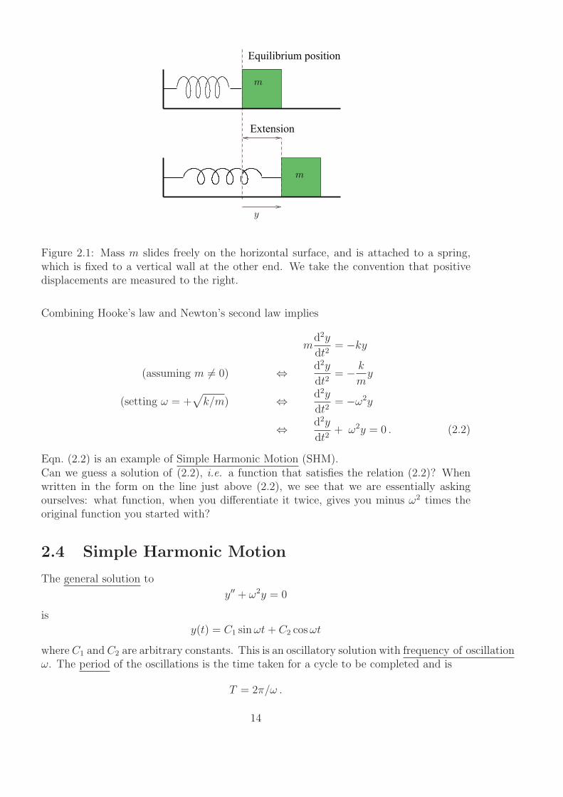
Consider a mass m kg on the end of a spring, as in Figure 2.1. With the initial conditionthat the mass is pulled to one side and then released, what do you expect to happen?
Hooke’s law implies that, provided y is not so large as to deform the spring, then therestoring force is
Fspring = −ky ,
where the constant k > 0 depends on the properties of the spring, for example its stiffness.
13
Equilibrium position
Extension
y
m
m
Figure 2.1: Mass m slides freely on the horizontal surface, and is attached to a spring,which is fixed to a vertical wall at the other end. We take the convention that positivedisplacements are measured to the right.
Combining Hooke’s law and Newton’s second law implies
md2y
dt2= −ky
(assuming m 6= 0) ⇔ d2y
dt2= − k
my
(setting ω = +√
k/m) ⇔ d2y
dt2= −ω2y
⇔ d2y
dt2+ ω2y = 0 . (2.2)
Eqn. (2.2) is an example of Simple Harmonic Motion (SHM).Can we guess a solution of (2.2), i.e. a function that satisfies the relation (2.2)? Whenwritten in the form on the line just above (2.2), we see that we are essentially askingourselves: what function, when you differentiate it twice, gives you minus ω2 times theoriginal function you started with?
2.4 Simple Harmonic Motion
The general solution to
y′′ + ω2y = 0
is
y(t) = C1 sinωt+ C2 cosωt
where C1 and C2 are arbitrary constants. This is an oscillatory solution with frequency of oscillationω. The period of the oscillations is the time taken for a cycle to be completed and is
T = 2π/ω .
14

Example 2.2. For the equationd2y
dt2+ 36y = 0
we have that ω2 = 36 and ω = 6 so the general solution is y(t) = C1 sin 6t+ C2 cos 6t.
Example 2.3. For the equation 16 d2y/dt2+y = 0 we first rewrite it as d2y/dt2+y/16 =0 . For this equation, ω2 = 1/16 and ω = 1/4 so the general solution is y = C1 sin
t4+
C2 cost4.
Question 2.3. Find the solution of
d2y
dt2+ 9y = 0
with y(0) = 2, dy/dt(0) = 0 . Find also the frequency of oscillations, the period ofoscillations, the amplitude of the solution, and the maximum velocity.Solution. The general solution to d2y/dt2 + 9y = 0 is
y(t) = C1 sin 3t+ C2 cos 3t . (2.3)
Differentiating (2.3) we get
dy
dt= 3C1 cos 3t− 3C2 sin 3t . (2.4)
Using y(0) = 2 in (2.3) and sin 0 = 0 , cos 0 = 1 , we obtain C2 = 2 .
Using dy/dt(0) = 0 in (2.4) we obtain C1 = 0 . Hence y(t) = 2 cos 3t. The frequency ofoscillations is 3 and the period is 2π/3 .The amplitude of the solution is the maximum displacement. From y(t) = 2 cos 3t theamplitude is 2 .
The velocity is dy/dt = −6 sin 3t so the the maximum velocity is 6 .
Question 2.4. Find the solution of
d2y
dt2+ 16y = 0
with y(0) = 0,dy
dt(0) = 12 .
Solution. The general solution to d2y/dt2 + 16y = 0 is
y(t) = C1 sin 4t+ C2 cos 4t . (2.5)
15
Differentiating (2.5) we get
dy
dt= 4C1 cos 4t− 4C2 sin 4t . (2.6)
Using y(0) = 0 in (2.5) and sin 0 = 0 , cos 0 = 1 we obtain C2 = 0 .
Usingdy
dt(0) = 12 in (2.6) we obtain 4C1 = 12 so C1 = 3 . Hence y(t) = 3 sin 4t.
2.5 Damped oscillations
Consider a more realistic spring which has resistance to motion.
In general, the frictional force or drag is proportional to velocity, i.e.
Ffriction = −Cdy
dt,
where C is a constant known as the drag or friction coefficient. The frictionalforce acts in a direction opposite to that of the motion and so C > 0.
Newton’s Second Law implies (adding the restoring and frictional forces together)
md2y
dt2= Fspring + Ffriction ,
i.e.
md2y
dt2= −ky − C
dy
dt.
Hence the damped oscillations of a spring are described by the differential equation
md2y
dt2+ C
dy
dt+ ky = 0. (2.7)
We show how to solve equation (2.7) in the next chapter.
2.6 ODE classification (revisited)
ODEs are classified according to order, linearity and homogeneity.
16

• Order. The order of a differential equation is the order of the highestderivative present in the equation.
• Linear or nonlinear. A second-order ODE is said to be linear if it can bewritten in the form
a(t)d2y
dt2+ b(t)
dy
dt+ c(t)y = f(t) , (2.8)
where the coefficients a(t), b(t) and c(t) can, in general, be functions oft. An equation that is not linear is said to be nonlinear. Note that linearODEs are characterised by two properties:
1. The dependent variable and all its derivatives are of first degree, i.e.the power of each term involving y is 1.
2. Each coefficient depends on the independent variable t only.
• Homogeneous or inhomogeneous. The linear differential equation (2.8) issaid to be homogeneous if f(t) ≡ 0; if f(t) 6≡ 0, the differential equationis said to be inhomogeneous.
Example 2.4. The differential equation
d2y
dt2+ 5
(dy
dt
)3
− 4y = et ,
is second order because the highest derivative is second order, and nonlinear because thesecond term on the left-hand side is cubic in dy/dt.
2.7 Homogeneous linear ODEs: The Principle of Su-
perposition
Consider the linear, second-order, homogeneous, ordinary differential equation
a(t)d2y
dt2+ b(t)
dy
dt+ c(t)y = 0 , (2.9)
where a(t), b(t) and c(t) are known functions.
17

• If y1(t) and y2(t) satisfy (2.9), then for any two constants C1 and C2, thePrinciple of Superposition says that
y(t) = C1y1(t) + C2y2(t) (2.10)
is a solution also.
• If y1(t) is not a constant multiple of y2(t), then the general solution of(2.9) takes the form (2.10).
2.8 Solving linear second-order constant-coefficient
homogeneous ODEs
2.8.1 Exponential solutions
We restrict ourselves here to the case when the coefficients a, b and c in (2.9) are constants,i.e. (2.9) is
ad2y
dt2+ b
dy
dt+ cy = 0 . (2.11)
Let us try to find a solution to (2.11) of the form
y = eλt . (2.12)
The reason for choosing the exponential function is that we know that solutions to linearfirst-order constant-coefficient ODEs always have this form for a specific value of λ thatdepends on the coefficients. So we’ll try to look for a solution to a linear second-orderconstant-coefficient ODE of the same form, where at the moment we will not specify whatλ is—with hindsight we will see that this is a good choice.Substituting (2.12) into (2.11) implies
ad2y
dt2+ b
dy
dt+ cy = aλ2eλt + bλeλt + ceλt
= eλt(aλ2 + bλ+ c)
which must = 0 .
Since the exponential function is never zero, i.e. eλt 6= 0, then we see that λ has to satisfythe auxiliary equation:
aλ2 + bλ+ c = 0 ,
then (2.12) will be a solution of (2.11). There are three cases we need to consider.
2.8.2 Case I: b2 − 4ac > 0
There are two real and distinct solutions to the auxiliary equation,
λ1 =−b+
√b2 − 4ac
2aand λ2 =
−b−√b2 − 4ac
2a,
18

and so two functions,eλ1t and eλ2t ,
satisfy the ordinary differential equation (2.11). The Principle of Superposition impliesthat the general solution is
y(t) = C1eλ1t + C2e
λ2t .
Question 2.5. Find the general solution to the ODE d2y/dt2 + 2dy/dt− 3y = 0.Solution. The auxiliary equation is λ2 + 2λ− 3 = 0.
b2 − 4ac = 4 + 12 = 16
so
λ =−2± 4
2hence λ = 1 or λ = −3 .
The general solution isy = C1e
t + C2e−3t.
2.8.3 Case II: b2 − 4ac = 0
In this case there is one real repeated root to the auxiliary equation, namely
λ1 = λ2 = − b
2a.
Hence we have one solution, which is
y(t) = eλ1t = e−b
2at.
However, there should be another independent solution (for a second-order differentialequation we should be able to impose two items of initial data to fix two constants,namely the coefficients of two independent solutions). It’s not obvious what it might be,but let’s make the educated guess
y = teλ1t
where λ1 is the same as above, i.e. λ1 = − b2a. Substituting this guess for the second
solution into our second-order differential equation,
⇒ ad2y
dt2+ b
dy
dt+ cy = a (λ2
1teλ1t + 2λ1e
λ1t) + b (eλ1t + λ1teλt) + c teλ1t
= eλ1t(t (aλ2
1 + bλ1 + c) + (2aλ1 + b))
which in fact = 0 ,
since we note that aλ21 + bλ1 + c = 0 and 2aλ1 + b = 0 because λ1 = −b/2a. Thus te−
b
2at
is another solution (which is clearly not a constant multiple of the first solution). ThePrinciple of Superposition implies that the general solution is
y = (C1 + C2t)e− b
2at .
19

Example 2.5. Find the general solution to the ODE d2y/dt2 + 4dy/dt+ 4y = 0 .
Solution. The auxiliary equation is λ2 + 4λ+ 4 = 0.
b2 − 4ac = 16− 16 = 0
so λ = −2 and the general solution is
y = (C1 + C2t) e−2t.
2.8.4 Case III: b2 − 4ac < 0
In this case, there are two complex roots to the auxiliary equation, namely
λ1 = p+ iq ,
λ2 = p− iq ,where p = − b
2aand q =
√
|b2 − 4ac|2a
. (2.13)
Hence the Principle of Superposition implies that the general solution takes the form
y(t) = A1eλ1t + A2e
λ2t
= A1e(p+iq)t + A2e
(p−iq)t
= A1ept+iqt + A2e
pt−iqt
= A1epteiqt + A2e
pte−iqt
= ept(A1e
iqt + A2e−iqt
)
(using Euler’s formula) = ept(A1
(cos qt+ i sin qt
)+ A2
(cos qt− i sin qt)
)
= ept((A1 + A2
)cos qt+ i
(A1 − A2
)sin qt)
), (2.14)
where:
1. We have used Euler’s formula
eiz ≡ cos z + i sin z ,
first with z = qt and then secondly with z = −qt, i.e. we have used that
eiqt = cos qt+ i sin qt and e−iqt = cos qt− i sin qt
since cos(−qt) = cos qt and sin(−qt) ≡ − sin qt;
2. A1 and A2 are arbitrary (and in general complex) constants—at this stage this meanswe appear to have a total of four constants because A1 and A2 both have real andimaginary parts. However we expect the solution y(t) to be real—the coefficientsare real and we shall pose real initial data.
The solution y(t) in (2.14) will be real if and only if
A1 + A2 = C1 , i(A1 − A2) = C2 ,
where C1 and C2 are real constants. Hence the general solution in this case has the form
y(t) = ept(C1 cos qt+ C2 sin qt) .
20
Question 2.6. Find the solution to d2y/dt2 + 4dy/dt+ 9y = 0.Solution. The auxiliary equation is λ2 + 4λ+ 9 = 0.
b2 − 4ac = 16− 36 = −20 = 20i2 so λ = (−4±√20i)/2 = −2±
√5i.
The general solution is y = e−2t(C1 cos
√5t+ C2 sin
√5t).
Question 2.7. Find the solution to the initial-value problem d2y/dt2 − dy/dt− 6y = 0
, with y(0) = 5 ,dy
dt(0) = 10.
Solution. The auxiliary equation is λ2 − λ− 6 = 0.
b2 − 4ac = 1 + 24 = 25 so that λ = 3 or λ = −2 .
The general solution isy = C1e
3t + C2e−2t.
Now dy/dt = 3C1e3t − 2C2e
−2t.
Using y(0) = 5,dy
dt(0) = 10 and e0 = 1,
C1 + C2 = 5 , 3C1 − 2C2 = 10 .
Solving these gives C1 = 4 and C2 = 1 so
y = 4e3t + e−2t.
Question 2.8. Find the solution to the initial-value problem d2y/dt2− 6dy/dt+9y = 0 ,
with y(0) = 2 ,dy
dt(0) = 1.
Solution. The auxiliary equation is λ2 − 6λ+ 9 = 0.
Then b2 − 4ac = 36− 36 = 0 so λ = 3 . The general solution is
y = (C1 + C2t) e3t.
Then dy/dt = 3 (C1 + C2t) e3t + C2e
3t .
Using y(0) = 2 anddy
dt(0) = 1, C1 = 2 and 3C1 + C2 = 1 so
y = (2− 5t) e3t.
21

Case Roots of Generalauxiliary equation solution
b2 − 4ac > 0 λ1,2 =−b±
√b2−4ac2a
y = C1eλ1t + C2e
λ2t
b2 − 4ac = 0 λ1,2 = − b2a
y =(C1 + C2t
)eλ1t
λ1,2 = p± iqb2 − 4ac < 0 y = ept
(C1 cos qt+ C2 sin qt
)
p = − b2a, q =
√|b2−4ac|2a
Table 2.1: Solutions to the linear second-order, constant-coefficient, homogeneous ODEad2y/dt2 + b dy/dt+ cy = 0.
Question 2.9. Find the solution to the initial-value problem d2y/dt2+6dy/dt+13y = 0 ,
with y(0) = −1 ,dy
dt(0) = 11.
Solution. The auxiliary equation is λ2 + 6λ+ 13 = 0.
b2 − 4ac = 36− 52 = −16 = 16i2 so
λ =−6± 4i
2= −3± 2i .
The general solution isy = e−3t (C1 cos 2t+ C2 sin 2t)
sody
dt= −3e−3t (C1 cos 2t+ C2 sin 2t) y + e−3t (−2C1 sin 2t+ 2C2 cos 2t) .
Using y(0) = −1,dy
dt(0) = 11, C1 = −1 − 3C1 + 2C2 = 11 so
y = e−3t (4 sin 2t− cos 2t) .
2.9 Practical example: damped springs
For the case of the damped spring note that in terms of the physical parameters a = m > 0,b = C > 0 and c = k > 0. Hence
b2 − 4ac = C2 − 4mk .
22
0 1 2 3 4 5 6 7 8 9 10−1
−0.5
0
0.5
1
y(t
)
(a) Overdamped (m=1, C=3, k=1)
y(0)=1, y′(0)=0
y(0)=−1, y′(0)=4
0 1 2 3 4 5 6 7 8 9 10−1
−0.5
0
0.5
1
y(t
)
(b) Critically damped (m=1, C=2, k=1)
y(0)=1, y′(0)=0
y(0)=−1, y′(0)=4
0 1 2 3 4 5 6 7 8 9 10−1
−0.5
0
0.5
1
t
y(t
)
(c) Underdamped (m=1, C=2, k=32)
y(0)=1, y′(0)=0
exponential
envelope
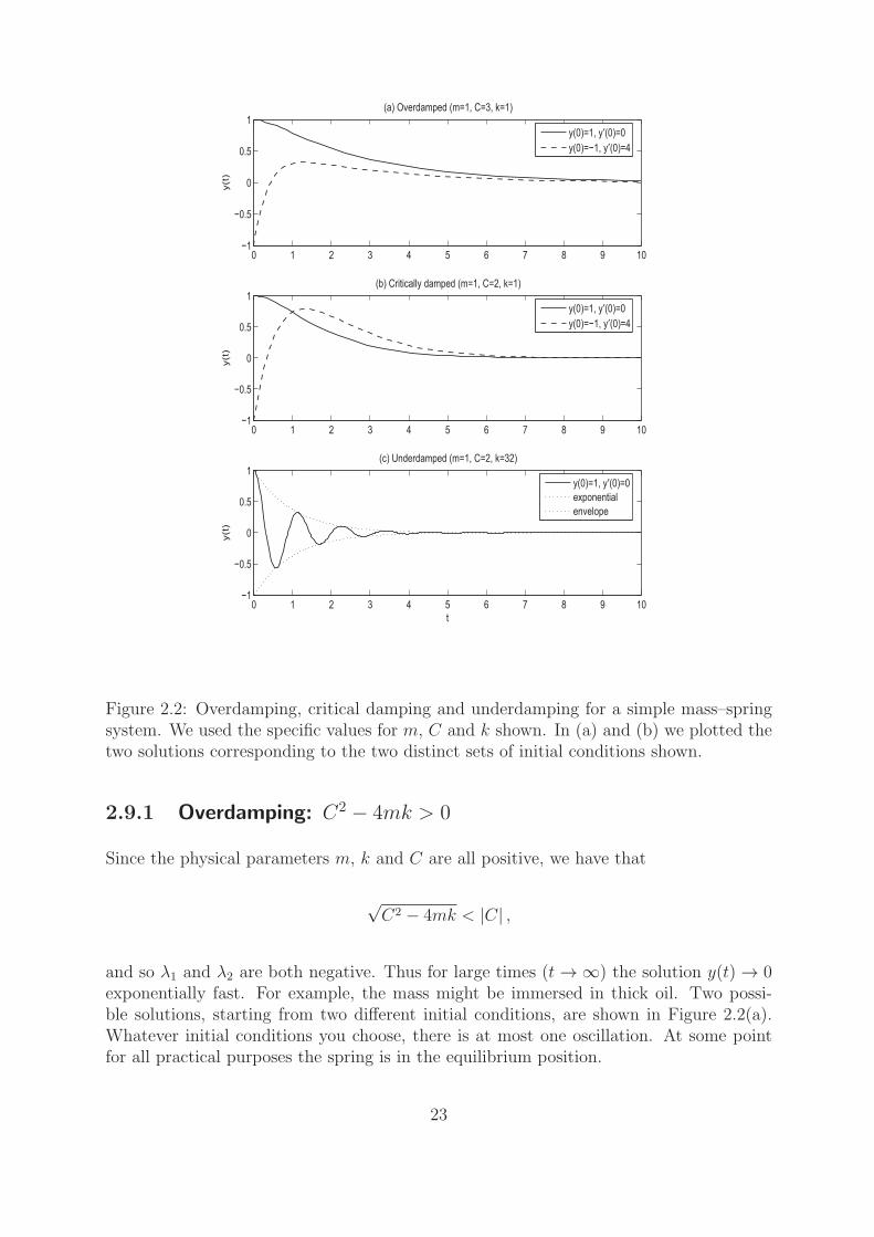
Figure 2.2: Overdamping, critical damping and underdamping for a simple mass–springsystem. We used the specific values for m, C and k shown. In (a) and (b) we plotted thetwo solutions corresponding to the two distinct sets of initial conditions shown.
2.9.1 Overdamping: C2 − 4mk > 0
Since the physical parameters m, k and C are all positive, we have that
√C2 − 4mk < |C| ,
and so λ1 and λ2 are both negative. Thus for large times (t → ∞) the solution y(t) → 0exponentially fast. For example, the mass might be immersed in thick oil. Two possi-ble solutions, starting from two different initial conditions, are shown in Figure 2.2(a).Whatever initial conditions you choose, there is at most one oscillation. At some pointfor all practical purposes the spring is in the equilibrium position.
23

2.9.2 Critical damping: C2 − 4mk = 0
In appearance—see Figure 2.2(b)—the solutions for the critically damped case look verymuch like those in Figure 2.2(a) for the overdamped case.
2.9.3 Underdamping: C2 − 4mk < 0
Since for the spring
p = − b
2a= − C
2m< 0 ,
the mass will oscillate about the equilibrium position with the amplitude of the os-cillations decaying exponentially in time; in fact the solution oscillates between theexponential envelopes which are the two dashed curves Aept and −Aept, where A =
+√
C21 + C2
2—see Figure 2.2(c). In this case, for example, the mass might be immersedin light oil or air.
24

2. Problems: 2nd Order Homogeneous ODEs
Problem 2.1. Find the general solutions to the following differential equations:
(a)d2y
dt2−9y = 0 ; (b)
d2y
dt2+dy
dt−6y = 0 ; (c)
d2y
dt2+8
dy
dt+16y = 0 .
Problem 2.2. Find the general solutions to the following differential equations:
(a)d2y
dt2+2
dy
dt+5y = 0 ; (b)
d2y
dt2−4
dy
dt+5y = 0 ; (c)
d2y
dt2−6
dy
dt+13y = 0 .
Problem 2.3. Find the solutions of :
(a)d2y
dt2+ 7
dy
dt+ 10y = 0, with y(0) = 0,
dy
dt(0) = 3;
(b)d2y
dt2+ 6
dy
dt+ 9y = 0, with y(0) = 1,
dy
dt(0) = 2;
(c)d2y
dt2+ 4
dy
dt+ 5y = 0, with y(0) = 3,
dy
dt(0) = 1.
Problem 2.4. Find the solution of d2y/dt2 + ω2y = 0 with y(0) = a, dy/dt (0) = 0.Write down the frequency, period and amplitude of oscillation.
Problem 2.5. The following represent the motion of oscillating springs.
1.d2y
dt2+ 4y = 0, y(0) = 5,
dy
dt(0) = 0,
2. 4d2y
dt2+ y = 0, y(0) = 10,
dy
dt(0) = 0,
3.d2y
dt2+ 6y = 0, y(0) = 4,
dy
dt(0) = 0,
4. 6d2y
dt2+ y = 0, y(0) = 20,
dy
dt(0) = 0.
Use the previous problem to determine which differential equation represents
(a) the spring oscillating most quickly (with the shortest period)?
(b) the spring oscillating with the largest amplitude?
(c) the spring oscillating most slowly (with the longest period)?
(d) the spring oscillating with the largest maximum velocity?
25
Answers
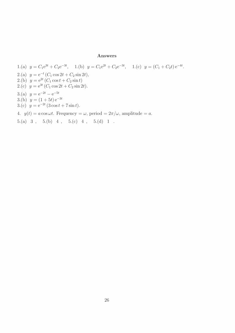
1.(a) y = C1e3t + C2e
−3t, 1.(b) y = C1e2t + C2e
−3t, 1.(c) y = (C1 + C2t) e−4t.
2.(a) y = e−t (C1 cos 2t+ C2 sin 2t),2.(b) y = e2t (C1 cos t+ C2 sin t)2.(c) y = e3t (C1 cos 2t+ C2 sin 2t).
3.(a) y = e−2t − e−5t
3.(b) y = (1 + 5t) e−3t
3.(c) y = e−2t (3 cos t+ 7 sin t).
4. y(t) = a cosωt. Frequency = ω, period = 2π/ω, amplitude = a.
5.(a) 3 , 5.(b) 4 , 5.(c) 4 , 5.(d) 1 .
26

Chapter 3
Inhomogeneous Linear ODEs
3.1 Examples of applications
Example 3.1. Forced spring systems What happens if our spring system (damped orundamped) is forced externally? For example, consider the following initial-value problemfor a forced harmonic oscillator (which models a mass on the end of a spring which isforced externally)
md2y
dt2+ C
dy
dt+ ky = f(t), y(0) =
dy
dt(0) = 0 .
Here y(t) is the displacement of the mass, m, from equilibrium at time t. The externalforcing f(t) could be oscillatory, say
f(t) = A sinωt ,
where A and ω are also (given) positive constants. We will see in this chapter how solutionsto such problems can behave quite dramatically when the frequency of the external forceω matches that of the natural oscillations ω0 = +
√
k/m of the undamped (C ≡ 0)system—undamped resonance! We will also discuss the phenomenon of resonance in thepresence of damping (C > 0).
3.2 Linear operators
Consider the general inhomogeneous second-order linear ODE
a(t)d2y
dt2+ b(t)
dy
dt+ c(t)y = f(t) . (3.1)
We can abbreviate the ODE (3.1) to
Ly(t) = f(t) , (3.2)
where L is the differential operator
L = a(t)d2
dt2+ b(t)
d
dt+ c(t) . (3.3)
27
We can re-interpret our general linear second-order ODE as follows. When we operate ona function y(t) by the differential operator L, we generate a new function of t:
Ly(t) = a(t)d2y
dt2(t) + b(t)
dy
dt(t) + c(t)y(t) .
To solve (3.2), we want the most general expression, y as a function of t, which is suchthat L operated on y gives f(t).
An operator L is said to be linear if
L(αy1 + βy2
)= αLy1 + βLy2 ,
for every y1 and y2, and all constants α and β.
As an example, the operator L in (3.3) is linear.
3.3 Solving inhomogeneous linear ODEs
Consider the linear second-order ODE
Ly = f . (3.4)
To solve this problem we first consider the solution to the associated homogeneous ODE:
LyCF = 0 . (3.5)
This solution is called a Complementary Function (CF). Since the ODE (3.5) is linear,second-order and homogeneous, we can always find an expression for the solution. In theconstant-coefficient case the solution has one of the forms given in Table 2.1. Now supposethat we can find a particular solution—often called the particular integral (PI)—of (3.4),i.e. some function, yPI, which satisfies (3.4):
LyPI = f .
Then the complete general solution of (3.4) is
y = yCF + yPI .
This must be the general solution because it contains two arbitrary constants (in the yCF
part) and satisfies the ODE, since, using that L is a linear operator,
L(yCF + yPI) = LyCF︸ ︷︷ ︸
=0
+LyPI︸︷︷︸
=f
= f .
Hence to summarise:
28
To solve an inhomogenous linear ODE of the form
Ly = f :
1. Find the general solution—the complementary function yCF—to the cor-responding homogeneous linear ODE
LyCF = 0 .
2. Find any solution—the particular integral yPI—to the full inhomogeneouslinear ODE
LyPI = f .
Then the general solution to the inhomogeneous linear ODE is
y = yCF + yPI .
3.4 Method of undetermined coefficients
We now need to know how to obtain a particular integral. For special cases of theinhomogeneity f(t) we use the method of undetermined coefficients. In the method ofundetermined coefficients we make an initial assumption about the form of the particularintegral yPI, but with the coefficients left unspecified. We substitute our guess for yPI intothe linear ODE, Ly = f , and attempt to determine the coefficients so that yPI satisfiesthe equation.
Question 3.1. Find the general solution of the linear ODE
d2y
dt2− 3
dy
dt− 4y = 3e2t .
Solution.
Step 1: Find the complementary function
Looking for a solution of the form eλt, the auxiliary equation is λ2− 3λ− 4 = 0 which hastwo real distinct roots λ1 = 4 and λ2 = −1 so that
yCF(t) = C1e4t + C2e
−t .
29

Inhomogeneity f(t) Try yPI(t)
eαt Aeαt
sinαt A sinαt+ B cosαt
cosαt A sinαt+ B cosαt
b0 + b1t+ b2t2 + · · ·+ bnt
n A0 + A1t+ A2t2 + · · ·+ Ant
n
eαt sin βt Aeαt sin βt+ Beαt cos βt
eαt cos βt Aeαt sin βt+ Beαt cos βt
Table 3.1: Method of undetermined coefficients. When the inhomogeneity f(t) hasthe form (or is any constant multiplied by this form) shown in the left-hand column, thenyou might try a yPI(t) of the form shown in the right-hand column. We can also makethe obvious extensions for combinations of the inhomogeneities f(t) shown.
30

Step 2: Find the particular integral
Assume that the particular integral has the form (using Table 3.1)
yPI(t) = Ae2t ,
where the coefficient A is yet to be determined. Substituting this form for yPI into theODE, we get
(4A− 6A− 4A)e2t = 3e2t ⇔ −6Ae2t = 3e2t .
Hence A must be −12and a particular solution is
yPI(t) = −12e2t .
Hence the general solution to the differential equation is
y(t) = C1e4t + C2e
−t
︸ ︷︷ ︸
yCF
−12e2t
︸ ︷︷ ︸
yPI
.
Question 3.2. Find the general solution of the linear ODE
d2y
dt2− 3
dy
dt− 4y = 2 sin t .
Solution.
Step 1: Find the complementary function
In this case, the complementary function is clearly the same as in the last example—thecorresponding homogeneous equation is the same—hence
yCF(t) = C1e4t + C2e
−t .
Step 2: Find the particular integral
Assume that yPI has the form (using Table 3.1)
yPI(t) = A sin t+B cos t ,
where the coefficients A and B are yet to be determined. Substituting this form for yPIinto the ODE implies
(−A sin t− B cos t)− 3(A cos t− B sin t)− 4(A sin t+B cos t) = 2 sin t
⇔ (−A+ 3B − 4A) sin t+ (−B − 3A− 4B) cos t = 2 sin t .
Equating coefficients of sin t and also cos t, we see that
−5A+ 3B = 2 and − 5B − 3A = 0 .
31

Hence A = − 517
and B = 317
and so
yPI(t) = − 517sin t+ 3
17cos t .
Thus the general solution is
y(t) = C1e4t + C2e
−t
︸ ︷︷ ︸
yCF
− 517sin t+ 3
17cos t
︸ ︷︷ ︸
yPI
.
Question 3.3. Find the solution to the initial value problem
d2y
dt2+ 4
dy
dt+ 5y = 20 , y(0) = 2 ,
dy
dt(0) = 7 .
Solution. Step 1 Solve d2y/dt2 + 4dy/dt+ 5y = 0 .
Auxiliary equation: λ2 + 4λ+ 5 = 0 .
Then b2 − 4ac = 16− 20 = −4 = 4i2 so
λ =−4± 2i
2= −2± i .
The general solution for the homogeneous equation is yCF = e−2t (C1 cos t+ C2 sin t).
Step 2 Find a particular integral of d2y/dt2 + 4dy/dt+ 5y = 20 .
Set y = C.
Then dy/dt = d2y/dt2 = 0 so 5C = 20 and C = 4. Hence a particular integral is yPI = 4.
Step 3 The general solution of d2y/dt2 + 4dy/dt+ 5y = 20 is
y = e−2t (C1 cos t+ C2 sin t) + 4
Step 4 Use the initial conditions for the general solution obtained in Step 3. Now
dy
dt= −2e−2t (C1 cos t+ C2 sin t) + e−2t (−C1 sin t+ C2 cos t) .
Using y(0) = 2,dy
dt(0) = 7,
C1 + 4 = 2 , −2C1 + C2 = 7 ,
so C1 = −2 and C2 = 3 . Hence
y = e−2t (3 sin t− 2 cos t) + 4 .
32

3.5 Degenerate inhomogeneities
Question 3.4. Find the general solution of the degenerate linear ODE
d2y
dt2+ 4y = 3 cos 2t .
Solution.
Step 1: Find the complementary function
First we solve the corresponding homogeneous equation
d2y
dt2+ 4y = 0 , (3.6)
to find the complementary function. Two solutions to this equation are sin 2t and cos 2t,and so the complementary function is
yCF(t) = C1 sin 2t+ C2 cos 2t ,
where C1 and C2 are arbitrary constants.
Step 2: Find the particular integral
Assume that yPI has the form
yPI(t) = A sin 2t+B cos 2t ,
where the coefficients A and B are yet to be determined. Substituting this form for yPIinto the ODE implies
(−4A sin 2t− 4B cos 2t) + 4(A sin 2t+B cos 2t) = 3 cos 2t
⇔ (4B − 4B) sin 2t+ (4A− 4A) cos 2t = 3 cos 2t .
Since the left-hand side is zero, there is no choice of A and B that satisfies this equation.Hence for some reason we made a poor initial choice for our particular solution yPI(t).This becomes apparent when we recall the solutions to the homogeneous equation (3.6) aresin 2t and cos 2t. These are solutions to the homogeneous equation and cannot possibly besolutions to the inhomogeneous case we’re considering. We must therefore try a slightlydifferent choice for yPI(t), for example,
yPI(t) = At cos 2t+Bt sin 2t .
Substituting this form for yPI into the ODE and cancelling terms imply
−4A sin 2t+ 4B cos 2t = 3 cos 2t .
Therefore, equating coefficients of sin 2t and cos 2t, we see that A = 0 and B = 34and so
yPI(t) =34t sin 2t .
33

Hence the general solution is
y(t) = C1 sin 2t+ C2 cos 2t︸ ︷︷ ︸
yCF
+ 34t sin 2t
︸ ︷︷ ︸
yPI
.
Occasionally such a modification will be insufficient to remove all duplications of thesolutions of the homogeneous equation, in which case it is necessary to multiply by t asecond time. For a second-order equation though, it will never be necessary to carry theprocess further than two modifications.
Question 3.5. Consider the following equation
d2y
dt2+ 16y = f(t) . (3.7)
(a) Find the general solution of equation (3.7) when f(t) = 0.
(b) Now suppose that f(t) = cos 2t . Write down what form for the particular integralyou would try.
(c) Now suppose that f(t) = sin 4t . Write down what form for the particular integralyou would try.
Solution.(a) y = C1 cos 4t+ C2 sin 4t .(b) y = A sin 2t+B cos 2t .(c) y = A t sin 4t+B t cos 4t .
Question 3.6. Consider the following equation
d2y
dt2− 36y = f(t) . (3.8)
(a) Find the general solution of equation (3.8) when f(t) = 0.
(b) Now suppose that f(t) = e4t. Write down what form for the particular integral youwould try.
(c) Now suppose that f(t) = e−6t. Write down what form for the particular integralyou would try.
Solution. For part (a), the auxiliary equation is λ2−36 = 0 so λ = ±6 and the generalsolution is
y = C1e6t + C2e
−6t.
(b) y = Ae4t.
(c) y = A te−6t.
34

Resonance
Example 3.2. Undamped resonance Consider the following initial value problem fora forced harmonic oscillator, which, for example, models a mass on the end of a springwhich is forced externally,
d2y
dt2+ ω2
0 y = 1mf(t), y(0) =
dy
dt(0) = 0 .
Here y(t) is the displacement of the mass m from equilibrium at time t, and ω0 =√
k/mis a positive constant representing the natural frequency of oscillation when no forcing ispresent. Suppose
f(t) = A sinωt
is the external oscillatory forcing, where A and ω are also positive constants.
The solution depends on if ω 6= ω0 or if ω = ω0.
If ω 6= ω0, a calculation shows that the solution is
y(t) =Aω
m(ω2 − ω20)
·( 1
ω0
sinω0t︸ ︷︷ ︸
natural oscillation
− 1
ωsinωt
︸ ︷︷ ︸
forced oscillation
)
, (3.9)
where the first oscillatory term represents the natural oscillations, and the second, theforced mode of vibration.
What happens when ω → ω0? If we naively take the limit ω → ω0 in (3.9) we see thatthe two oscillatory terms combine to give zero, but the denominator in the multiplicativeterm
Aω
m(ω2 − ω20)
also goes to zero. This implies we should be much more careful.
If ω = ω0 the solution to the initial-value problem is
y(t) =A
2mω0
·( 1
ω0
sinω0t︸ ︷︷ ︸
natural oscillation
− t cosω0t︸ ︷︷ ︸
resonant term
)
. (3.10)
The important aspect to notice is that when ω = ω0, the second term ‘t cosω0t’ growswithout bound (the amplitude of these oscillations grows like t) and this is the “signatureof undamped resonance”.
Damped resonance
Suppose we introduce damping into our simple spring system so that the coefficient offriction C > 0. In the overdamped, critically damped or underdamped cases the com-plementary function is always exponentially decaying in time. We call this part of the
35
solution the transient solution—it will be significant initially, but it decays to zero ex-ponentially fast. The contribution to the solution from the particular integral, whicharises from the external forcing, cannot generate unbounded resonant behaviour for anybounded driving oscillatory force. However the amplitude of the forced oscillations of thesolution (from the particular integral, which is potentially the only significant componentfor large times) does have a global maximum at a given practical resonance frequency.
36

3. Problems: 2nd Order Inhomogeneous ODEs
Problem 3.1. For the following inhomogeneous differential equations, determine thecomplimentry function and write down what form for the particular integral you wouldtry (just write it down, there’s no need to do any calculations):
(a)d2y
dt2+16y = sin 3t ; (b)
d2y
dt2+16y = cos 4t ; (c)
d2y
dt2−25y = e4t ; (d)
d2y
dt2−25y = e−5t .
Problem 3.2. Find the general solution to the inhomogeneous differential equations:
(a) d2y/dt2 + 4y = sin 3t ; (b) d2y/dt2 − 9y = 16e−t ;(c) d2y/dt2 − 5dy/dt+ 6y = 2 sin 4t ; (d) d2y/dt2 − 5dy/dt+ 6y = e−2t ;(e) d2y/dt2 + 2dy/dt+ y = t ; (f) d2y/dt2 + 4y = sin 2t .
Problem 3.3. Solved2y
dt2− y = 12e2t, with y(0) = 4,
dy
dt(0) = 10.
Problem 3.4. Solved2y
dt2− 5
dy
dt+ 6y = cos 3t, with y(0) = 0,
dy
dt(0) = 5.
Problem 3.5. The charge Q(t) in a simple electrical circuit, consisting of a coil withinductance L, a capacitance C and resistance R, satisfies
Ld2Q
dt2+R
dQ
dt+
1
CQ = V (t)
where V (t) is an imposed voltage. Find Q(t), given that L = 1, R = 2, C = 1/5,
Q(0) = Q0,dQ
dt(0) = 0, and the voltage is V (t) = e−t sin 3t.
Problem 3.6. The landing gear of a plane, consisting of a spring and a damper, is testedusing a drop test, where the response of a subsystem of the landing gear is subjected to aninstantaneous force representative of a plane landing. The spring force Fspring, modelledusing Hooke’s law, and the damper force, Fdamper are as follows:
Fspring = kx , Fdamper = Bdx
dt,
where x is the height and t is time.
Applying Newton’s 2nd law, ’F = ma’, (and the force due to gravity) we get
mg − Bdx
dt− kx = m
d2x
dt2⇒ d2x
dt2+
B
m
dx
dt+
k
mx = g.
Given the intial conditions x(0) = 0 and dxdt
= V when t = 0 and that m = 50, k = 312.5,B = 150 and we approximate g = 10 find the solution to the initial value problem (youranswer will be in terms of V ).
37

Answers
1.(a) y = A sin 3t+B cos 3t ; 1.(b) y = At sin 4t+Bt cos 4t ; 1.(c) y = Ae4t ;1.(d) y = Ate−5t.
2.(a) y = C1 sin 2t+ C2 cos 2t− 15sin 3t; 2.(b) y = C1e
3t + C2e−3t − 2e−t.
2(c) y = C1e3t + C2e
2t + 225cos 4t− 1
25sin 4t; 2.(d) y = C1e
3t + C2e2t + 1
20e−2t;
2.(e) y = (C1 + C2t) e−t + t− 2; 2.(f) y = C1 sin 2t+C2 cos 2t− t
4cos 2t.
3. y = et − e−t + 4e2t .
4. y = 316e3t − 67
13e2t − 5
78sin 3t− 1
78cos 3t .
5. Q = e−t
(
Q0 cos 2t+
(5Q0 + 3
10
)
sin 2t
)
− 1
5e−t sin 3t.
6. x = e−1.5t (−1.6 cos 2t+ (0.5V − 1.2) sin 2t) + 1.6.
38
Chapter 4
Partial Differentiation
To date most functions have had only one variable; for example,
• “y is a function of x”,
• “position is a function of time”.
However functions can have two or more variables — they often do in physical situations!
Partial differentiation gives us a way to generalise differentiation for functions of severalvariables.
4.1 Reminder of derivatives of functions of a single
variable
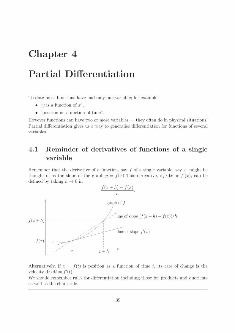
Remember that the derivative of a function, say f of a single variable, say x, might bethought of as the slope of the graph y = f(x) This derivative, df/dx or f ′(x), can bedefined by taking h → 0 in
f(x+ h)− f(x)
h.
line of slope (f (x + h)− f (x))/h
line of slope f ′(x)
f (x + h)
graph of f
x + h
f (x)
x
Alternatively, if z = f(t) is position as a function of time t, its rate of change is thevelocity dz/dt = f ′(t).
We should remember rules for differentiation including those for products and quotientsas well as the chain rule.
39

Question 4.1. Let y = x ln x. Find dy/dx.
Solution. Use the product rule: if y(x) = u(x)v(x) thendy
dx=
d
dx(uv) = u
dv
dx+ v
du
dx.
Here we let u = x and v = ln x so du/dx = 1 and dv/dx = 1/x. Then
dy
dx=
d
dx(x ln x) = x · (1/x) + (ln x) · 1 = 1 + ln x .
Question 4.2. Find dy/dx where y = x2 cos x.Solution. Let u = x2 and v = cosx so du/dx = 2x and dv/dx = − sin x. Thus theproduct rule gives
dy
dx= −x2 sin x+ 2x cos x .
Question 4.3. Findd
dx
( x
ex
)
.
Solution. This time we use the quotient rule:d
dx
(u
v
)
=v dudx
− udvdx
v2. Letting u = x
and v = ex we have du/dx = 1 and dv/dx = ex. Thus the quotient rule gives
d
dx
( x
ex
)
=ex − xex
(ex)2= (1− x)e−x .
Note that x/ex is the same as xe−x which can be differentiated using the product rule.
Question 4.4. Let y = 2 cos2 x. Find dy/dx.
Solution. Now use the chain rule:dy
dx=
du
dx
dy
du. Writing y = 2(cos x)2 = 2u2 with
u = cos x we have du/dx = − sin x and dy/du = 4u. Thus the chain rule gives
dy
dx=
du
dx
dy
du= (− sin x).4u = −4 sin x cos x .
Question 4.5. A particle moves along a line y = 6x−3 in such a way that its x coordinateat time t is x = 3t+ 5. Find the instantaneous velocity in the y direction.
Solution. It is possible to use the chain rule:dy
dt=
dy
dx
dx
dt= 6× 3 = 18.
(Alternatively the expression for x can be substituted into that for y: y = 6(3t+5)− 3 =18t+ 27. Then dy/dt = 18.)
4.2 Partial derivatives of functions of two variables
Example 4.1. If we definef(x, y) = xy2 + y3
then f is a function of two variables, namely x and y.
40

Example 4.2. Consider the volume V of box with sides x, y and z:
✏✏✏✏✏✏✏✏✏✏
✏✏✏✏✏
xy
z
Then V = V (x, y, z) = xyz is a function of three variables.
Example 4.3. Consider the function f of two variables given by
f(x, y) = x2 + 3xy − y2.
We might be interested in how rapidly this varies as either x or y changes. In particular,fixing y and regarding f purely as depending upon x we can then differentiate f withrespect to x. Similarly, we can regard x as fixed to determine a derivative of f withrespect to y. We then get the two partial derivatives
∂f
∂x= 2x+ 3y and
∂f
∂y= 3x− 2y.
Note the use of the different style “d”, ∂, when we take partial derivatives.These partial derivatives can be got from:
∂f
∂x(x, y) = lim
h→0
f(x+ h, y)− f(x, y)
h; (4.1)
∂f
∂y(x, y) = lim
h→0
f(x, y + h)− f(x, y)
h. (4.2)
It can be seen from these that
∂f/∂x is calculated by regarding y as a constant and using the normal rules ofdifferentiation to differentiate with respect to x;
∂f/∂y is calculated by regarding x as a constant and using the normal rules ofdifferentiation to differentiate with respect to y.
41

Example 4.4. Consider the function f of two variables given by
f(x, y) = x sin y + ye2x.
Then∂f
∂x= sin y + 2ye2x and
∂f
∂y= x cos y + e2x.
For f a function of x and y, we might visualise its graph as a surface in three-dimensionalspace. ∂f/∂x is then the slope of this surface in the x direction (broken line in the figurebelow) while ∂f/∂y is the slope in the y direction (dotted line).
00.2
0.40.6
0.81
0
0.2
0.4
0.6
0.8
10
0.5
1
1.5
2
2.5
xy
f
Alternatively, still for a function of two variables f(x, y), we might plot curves givingconstant values of f in the x - y plane. (Like contour lines on a map.)
Example 4.5. Taking f(x, y) = x2 + y2, f = constant, say c, if x2 + y2 = r2 = c ≥ 0,
with r the distance of the point (x, y) from the origin.
f = 0
f = r21
f = r22
42

Question 4.6. Find ∂f/∂x and ∂f/∂y where f(x, y) = 3y/(y + cos x).Solution. For ∂f/∂x we regard y as a constant and use the quotient rule:
∂f
∂x=
∂
∂x
(3y
y + cos x
)
=(y + cos x) ∂
∂x(3y)− 3y ∂
∂x(y + cosx)
(y + cos x)2
=(y + cosx)× 0− 3y × (− sin x)
(y + cos x)2=
3y sin x
(y + cos x)2.
For ∂f/∂y we regard x as a constant an use the quotient rule:
∂f
∂y=
∂
∂y
(3y
y + cos x
)
=(y + cos x) ∂
∂y(3y)− 3y ∂
∂y(y + cos x)
(y + cos x)2
=(y + cos x)× 3− 3y × 1
(y + cos x)2=
3 cos x
(y + cos x)2.
4.3 Higher-order partial derivatives
So far we have only seen first-order partial derivatives – taking a single derivative at a time.As with ordinary differentiation we can do repeated differentiation, taking derivatives ofderivatives, to get higher-order derivatives.
Example 4.6. For the function
f(x, y) = exy + x2y
the first-order partial derivatives are
∂f
∂x= yexy + 2xy and
∂f
∂y= xexy + x2.
We can now compute the second-order partial derivatives:
∂2f
∂x2=
∂
∂x
(∂f
∂x
)
=∂
∂x
(
yexy + 2xy)
= y2exy + 2y
∂2f
∂y2=
∂
∂y
(∂f
∂y
)
=∂
∂y
(
xexy + x2)
= x2exy
∂2f
∂y∂x=
∂
∂y
(∂f
∂x
)
=∂
∂y
(
yexy + 2xy)
= y · xexy + exy + 2x = (xy + 1)exy + 2x
∂2f
∂x∂y=
∂
∂x
(∂f
∂y
)
=∂
∂x
(
xexy + x2)
= x · yexy + exy + 2x = (xy + 1)exy + 2x .
43

It is a general rule that for “reasonable” functions,
∂2f
∂x∂y=
∂2f
∂y∂x. (4.3)
For “mixed” derivatives of functions which you meet in this course, the orderin which the derivatives are taken does not matter.
Question 4.7. Let f(x, y) = ln(x2 + y2).
(i) Verify that∂2f
∂x∂y=
∂2f
∂y∂x.
(ii) Show that∂2f
∂x2+
∂2f
∂y2= 0.
Solution. Using the chain rule (regarding the variable we’re not differentiating withrespect to as being constant), we have that ∂f/∂x = 2x/(x2 + y2) and ∂f/∂y = 2y/(x2 +y2). The quotient rule now gives
∂2f
∂x2=
∂
∂x
(∂f
∂x
)
=(x2 + y2).2− 2x.2x
(x2 + y2)2=
2(y2 − x2)
(x2 + y2)2,
∂2f
∂y∂x=
∂
∂y
(∂f
∂x
)
=(−2y).2x
(x2 + y2)2=
−4xy
(x2 + y2)2,
∂2f
∂y2=
∂
∂y
(∂f
∂y
)
=(x2 + y2).2− 2y.2y
(x2 + y2)2=
2(x2 − y2)
(x2 + y2)2,
∂2f
∂x∂y=
∂
∂x
(∂f
∂y
)
=(−2x).2y
(x2 + y2)2=
−4xy
(x2 + y2)2,
Hence it can be seen that (i) ∂2f/∂x∂y = ∂2f/∂y∂x and that (ii) ∂2f/∂x∂y = ∂2f/∂y∂x.
Question 4.8. Find∂2w
∂x∂ygiven that w(x, y) = xy +
ey
y2 + 1.
Solution. This is made simpler by reversing the order of differentiation:
∂2w
∂x∂y=
∂2w
∂y∂x=
∂
∂y
(∂w
∂x
)
=∂
∂yy = 1 .
4.4 Directional Derivatives
The value of ∂f∂x
at a point (a, b) gives the gradient of f(x, y) in the x-direction at (a, b).
Similarly, the value of ∂f∂y
at a point (a, b) gives the gradient of f(x, y) in the y-direction
at (a, b).
44
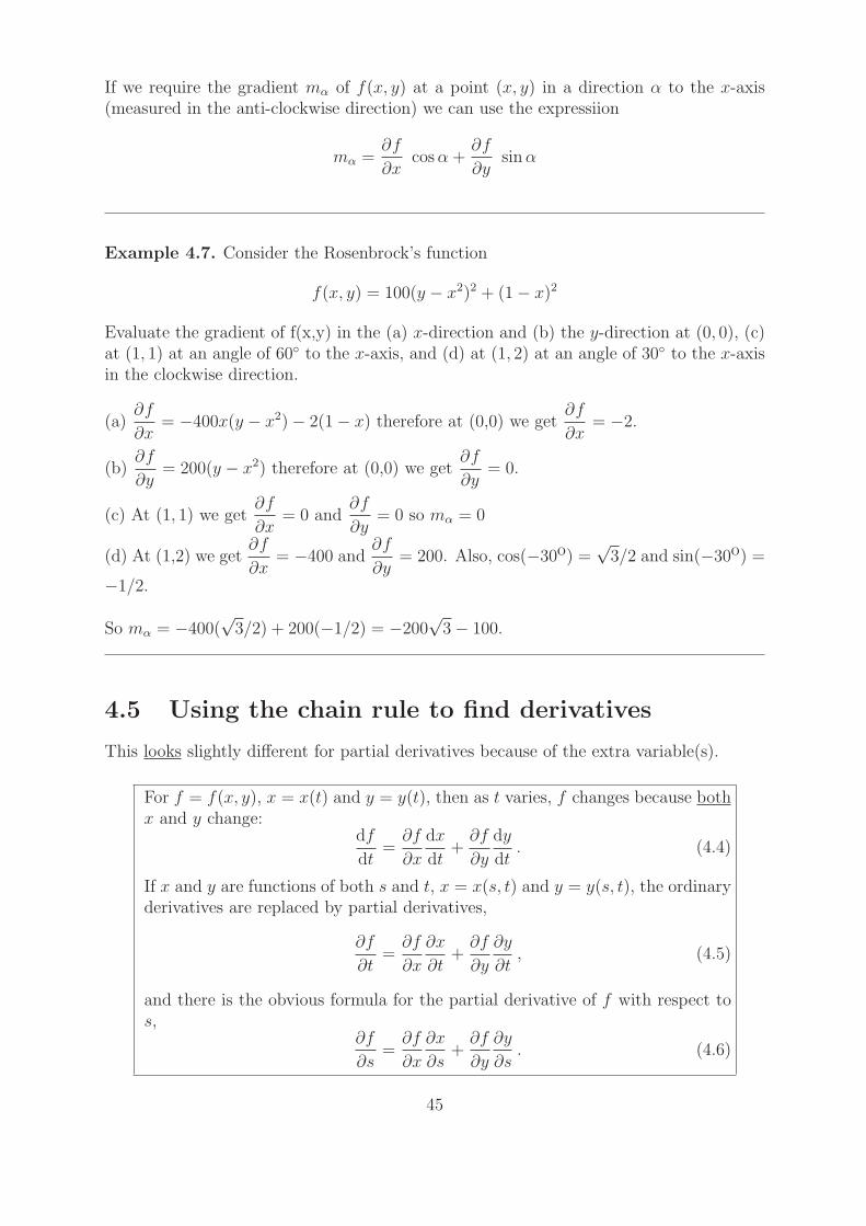
If we require the gradient mα of f(x, y) at a point (x, y) in a direction α to the x-axis(measured in the anti-clockwise direction) we can use the expressiion
mα =∂f
∂xcosα +
∂f
∂ysinα
Example 4.7. Consider the Rosenbrock’s function
f(x, y) = 100(y − x2)2 + (1− x)2
Evaluate the gradient of f(x,y) in the (a) x-direction and (b) the y-direction at (0, 0), (c)at (1, 1) at an angle of 60◦ to the x-axis, and (d) at (1, 2) at an angle of 30◦ to the x-axisin the clockwise direction.
(a)∂f
∂x= −400x(y − x2)− 2(1− x) therefore at (0,0) we get
∂f
∂x= −2.
(b)∂f
∂y= 200(y − x2) therefore at (0,0) we get
∂f
∂y= 0.
(c) At (1, 1) we get∂f
∂x= 0 and
∂f
∂y= 0 so mα = 0
(d) At (1,2) we get∂f
∂x= −400 and
∂f
∂y= 200. Also, cos(−30o) =
√3/2 and sin(−30o) =
−1/2.
So mα = −400(√3/2) + 200(−1/2) = −200
√3− 100.
4.5 Using the chain rule to find derivatives
This looks slightly different for partial derivatives because of the extra variable(s).
For f = f(x, y), x = x(t) and y = y(t), then as t varies, f changes because bothx and y change:
df
dt=
∂f
∂x
dx
dt+
∂f
∂y
dy
dt. (4.4)
If x and y are functions of both s and t, x = x(s, t) and y = y(s, t), the ordinaryderivatives are replaced by partial derivatives,
∂f
∂t=
∂f
∂x
∂x
∂t+
∂f
∂y
∂y
∂t, (4.5)
and there is the obvious formula for the partial derivative of f with respect tos,
∂f
∂s=
∂f
∂x
∂x
∂s+
∂f
∂y
∂y
∂s. (4.6)
45

Question 4.9. Suppose f(x) = ex and x(t) = t3. Compute df/dt.Solution. As a function of t we have f(t) = et
3
. Now
df
dx= ex and
dx
dt= 3t2
so the chain rule givesdf
dt=
df
dx
dx
dt= ex · 3t2 = 3t2et
3
.
Example 4.8. Suppose that f(x, y) = yex, where x = sin t and y = t2. Then
∂f
∂x= yex,
∂f
∂y= ex and
dx
dt= cos t ,
dy
dt= 2t.
Using the chain rule it follows that
df
dt=
∂f
∂x
dx
dt+
∂f
∂y
dy
dt= yex · cos t+ ex · 2t = t2esin t cos t+ 2tesin t.
Note that, as a function of t we have
f(t) = t2esin t.
We can also compute df/dt from this expression (using the product and chain rules forone variable — do this to see that the same result is obtained!)
Question 4.10. Suppose
f(x, y) = x3 − y2
where x = st and y = s/t. Find∂f
∂t.
Solution. We have∂f
∂x= 3x2,
∂f
∂y= −2y
and∂x
∂t= s,
∂y
∂t= − s
t2.
Using the chain rule it follows that
∂f
∂t=
∂f
∂x
∂x
∂t+
∂f
∂y
∂y
∂t= 3x2 · s+ (−2y)
(
− s
t2
)
= 3(st)2s+ 2(s/t)(s/t2) = 3s3t2 + 2s2/t3 .
46

4.6 Functions of many variables
Partial differentiation extends easily to functions of many variables.
• To calculate the partial derivative with respect to a certain variable keep all theother variables constant.
• For mixed derivatives the order (generally) doesn’t matter!
• The chain rule contains more terms.
Example 4.9. If f ≡ f(x, y, z) where x, y, z are functions of s, t then
∂f
∂t=
∂f
∂x
∂x
∂t+
∂f
∂y
∂y
∂t+
∂f
∂z
∂z
∂t.
Similarly for∂f
∂s.
Example 4.10. Consider the function of four variables
f(x, y, z, t) = xy + z2t.
Here there are four first-order partial derivatives
∂f
∂x= y,
∂f
∂y= x,
∂f
∂z= 2zt,
∂f
∂t= z2.
We can also compute higher-order derivatives; for example
∂2f
∂z∂t=
∂
∂z
(∂f
∂t
)
=∂
∂z(z2) = 2z.
Note that we also have∂2f
∂t∂z= 2z. (Check this!)
Question 4.11. Let f(x, y, z) = 2x2 + y2 + 3z and let x = uv, y = 2v and z = v + ln u.Find ∂f/∂u and ∂f/∂v.Solution.
∂f
∂u=
∂f
∂x
∂x
∂u+
∂f
∂y
∂y
∂u+
∂f
∂z
∂z
∂u= 4x · v + 2y · 0 + 3 · 1/u = 4uv2 + 3/u .
∂f
∂v=
∂f
∂x
∂x
∂v+
∂f
∂y
∂y
∂v+
∂f
∂z
∂z
∂v= 4x · u+ 2y · 2 + 3 · 1 = 4u2v + 8v + 3 .
47
4.7 Partial differential equations
• A partial differential equation (or PDE ) is an equation involving several variables,a function of these variables and its partial derivatives.
• PDEs arise in very many physical situations. They describe how physical quantitieschange with respect to several different variables.
• In this course we will only show that a given function is a solution of a given PDE— a straightforward calculation!
Example 4.11. An example of a PDE is
3y2∂U
∂x+
∂U
∂y= 2U.
where U is a function of x and y.
Example 4.12. Another example of a PDE is
∂2w
∂t2+ 2
∂2w
∂x∂y= 4w.
where w is a function of x, y and t.
48

Question 4.12. Show that u(x, y) = e2x+y2 is a solution of the partial differential equation
y2∂2u
∂x2+
1
y
∂u
∂y− ∂2u
∂y2= 0 .
Solution. Calculating the partial derivatives, we have
∂u
∂y= 2ye2x+y2 ,
∂2u
∂y2= 4y2e2x+y2 + 2e2x+y2 ,
∂u
∂x= 2e2x+y2 ,
∂2u
∂x2= 4e2x+y2 .
Thus
y2∂2u
∂x2+
1
y
∂u
∂y− ∂2u
∂y2= y2 × 4e2x+y2 +
1
y× 2ye2x+y2 −
(
4y2e2x+y2 + 2e2x+y2)
= 0 .
Example 4.13. Let w(x, t) denote the displacement of the point at x on a string at time t.A wave moving along the string with speed c can be modelled by the one-dimensional wave equation:
∂2w
∂t2= c2
∂2w
∂x2. (4.7)
A slice of the graph with t fixed shows us the shape of the string at that time t. Thefigure shows three such slices:
x
u
t = Tt = 0t = −T
u = f (x− cT )
cT
u = f (x)
cT
u = f (x + cT )
A slice of the graph with x fixed would show us how the point at x on the string moveswith time.
49

Question 4.13. Show that the function
w(x, t) = cos(x− ct)
is a solution of the 1D wave equation.Solution. Direct calculations give
∂w
∂t= c sin(x− ct),
∂2w
∂t2= −c2 cos(x− ct)
and∂w
∂x= − sin(x− ct),
∂2w
∂x2= − cos(x− ct).
It follows that∂2w
∂t2= c2
∂2w
∂x2,
as required.
Note: The alternative notation of subscripts is also used for partial differentiation, sothat fx means ∂f/∂x, uyz is the same as ∂2u/∂y ∂z, etc.
50

4. Problems: Partial Differentiation
Problem 4.1. Find ∂f/∂x and ∂f/∂y for each of the following functions:
(a) 3x+ 4y (b) xy3 + x2y2 (c) x3y + ex
(d) xe2x+3y (e) (x− y)/(x+ y) (f) 2x sin(x2y) .
Problem 4.2. Find ∂f/∂x, ∂f/∂y and ∂f/∂z for f(x, y, z) = x cos z + x2y3ez.
Problem 4.3. Find ∂2f/∂x2 and ∂2f/∂y2, and check that ∂2f/∂x∂y = ∂2f/∂y∂x for
(i) f(x, y) = x2 sin y + y2 cos x ; (ii) f(x, y) =(y
x
)
ln x .
Problem 4.4. Calculate the gradient for the Rosenbrock’s function
f(x, y) = 100(y − x2)2 + (1− x)2
at (a) (x, y) = (−1, 1) at an angle α = 45◦ to the x-axis is an anti-clockwise direction.(b) (x, y) = (−1, 1) at an angle α = 45◦ to the x-axis is an clockwise direction.(c) (x, y) = (1, 2) at an angle α = 80◦ to the x-axis is an anti-clockwise direction.
Problem 4.5. Suppose that f(x, y) =1
x2 + y2, x = r cos t and y = r sin t. Find ∂f/∂r
and ∂f/∂t.
Problem 4.6. Suppose that f(x, y) = x2 + xy − y2, x = r cos θ and y = r sin θ. Find∂f/∂r and ∂f/∂θ, (i) by direct substitution and (ii) by using the chain rule.
Problem 4.7. Suppose that f(x, y) = x3y − y3x, x = uv and y = u/v. Find ∂f/∂u and∂f/∂v.
Problem 4.8. Suppose that f(x, y, z) = 2y − sin xz, x = 3t, y = et−1 and z = ln t. Finddf/dt.
Problem 4.9. Suppose that f(x, y) = x2 + xy + y2, x = uv and y = u/v. Show that
u∂f
∂u+ v
∂f
∂v= 2x
∂f
∂xand u
∂f
∂u− v
∂f
∂v= 2y
∂f
∂y.
Is the same true for f(x, y) = x sin y + y sin x?
Problem 4.10. Show that u = ln(1+xy2) is a solution of the partial differential equation
2∂2u
∂x2+ y3
∂2u
∂x∂y= 0 .
Problem 4.11. Show that u(x, y) = x2 cosh(1+xy2) is a solution of the partial differentialequation
2x∂u
∂x− y
∂u
∂y− 4u = 0 .
Problem 4.12. Show that u(x, t) = ln(2x + 2ct) is a solution of the one-dimensionalwave equation
∂2u
∂t2= c2
∂2u
∂x2
51
Answers
3.(i) 2 sin y − y2 cosx, 2 cos x− x2 sin y.
3.(ii)y
x3(2 ln x− 3), 0.
4. (a) −2√2 = −2.828, (b) −2
√2 = −2.828, (c) 127.5
5. −2/r3, 0.
6. 2r(cos2 θ + cos θ sin θ − sin2 θ), r2(cos2 θ − sin2 θ − 4 cos θ sin θ).
7. 4u3v2 − 4u3/v2, 2u4v + 2u4/v3.
8. −3 cos(3t ln t)(1 + ln t) + 2et−1.
52

Chapter 5
Maxima and Minima
As before, we first look at the one-variable case
Question 5.1. Find the stationary points of the function
f(x) =x3
3− x+ 2.
Solution. We have f ′(x) = x2 − 1 so
f ′(x) = 0 ⇐⇒ x2 − 1 = 0 ⇐⇒ x2 = 1 ⇐⇒ x = ±1 .
Thus f has two stationary points, one at x = −1 and the other at x = 1.
Example 5.1. Returning to the previous example we have f ′′(x) = 2x. The secondderivative test then gives us the following information:
Stationary point x f ′′(x) Nature of stationary point
−1 −2 < 0 local maximum
+1 +2 > 0 local minimum
The graph of f looks something like the following:
✲x
✻y
s
−1
83
s
1
43
2
53

Example 5.2. Consider the function f(x) = x4. Then f ′(x) = 4x3 so the stationarypoints of f occur when
f ′(x) = 0 ⇐⇒ 4x3 = 0 ⇐⇒ x = 0.
Now f ′′(x) = 12x2 so at the stationary point x = 0 we get f ′′(x) = 0; it follows that wecannot use the second derivative test to determine the nature of the stationary point!However f(x) = x4 = (x2)2 ≥ 0 for all values of x while f(0) = 0. It follows that x = 0must be a local minimum.
Question 5.2. You have been asked to design a 1-litre oil can shaped like a cylinder.What dimensions will use the least material?Solution. Consider the oil can:
....................................................
..................................
................................................................................................................................................................................................................................................................................................................................................................................. ............. .............. ................ .................. ................... ..................... ...................... ................................. .................................. .................................. ................................. ...................... .....................
.........................................................................................................
.......................... ............. .............. ................ .................. ................... ..................... ...................... ................................. .................................. .................................. ................................. ...................... .................................................................................................................................................
.........................
.......................................................................................................................................................
s ✲✛ r
✻
❄
h
The amount of material need to make the oil can is simply A, the surface area of thecylinder; we wish to minimise A whilst keeping the volume of the can, V equal to 1 l =1000 cm3.Now
A = area of ends + area of cylinder wall
= 2πr2 + 2πrh.
On the other hand
V = πr2h = 1000 so h =1000
πr2.
It follows that
A = A(r) = 2πr2 + 2πr × 1000
πr2= 2πr2 +
2000
r.
Therefore
A′(r) = 4πr − 2000
r2
so
A′(r) = 0 ⇐⇒ 4πr =2000
r2⇐⇒ r =
3
√
500
π.
54

Thus A has a stationary point when r = 3
√
500/π; we need to check the nature of thisstationary point. Now
A′′(r) = 4π +4000
r3
so when r = 3
√
500/π we get
A′′(r) = 4π + 4000× π
500= 12π > 0.
Thus the stationary point is a local minimum. It follows that use of material is minimisedif we make a cylindrical oil can with radius
r = 3
√
500/π ≈ 5.42 cm.
Two variables are more complicated! But we shall clearly still need first derivatives tovanish, so, for f = f(x, y), we need both
∂f
∂x(x, y) = 0 and, simultaneously,
∂f
∂y(x, y) = 0 . (5.1)
One thing we shall certainly want is an equivalent of the second-derivative test.
Example 5.3. What sort stationary points might (i) f(x, y) = x2 + y2, (ii) g(x, y) =−x2 − 2y2, (iii) h(x, y) = x2 + 4xy + y2 have?
The first two are fairly obvious: For (x, y) 6= (0, 0), f > 0 and g < 0 but f = g = 0 if(x, y) = (0, 0). f clearly has a minimum at x = y = 0 while g has a maximum there.
The third one is not so straightforward, although it’s apparent that ∂h/∂x = 2(x + 2y)and ∂h/∂y = 2(2x + y) are only simultaneously zero at the origin. Taking x = 0 givesh = y2 ≥ 0, while if y = 0, h = x2 ≥ 0. However, we can complete the square to geth = (x+ 2y)2 − 3y2. It can now be seen that if x 6= 0 = y then h > 0 but if x = −2y 6= 0then h ≤ 0. Depending upon which direction we move away from the stationary point atx = y = 0, the graph of h = h(x, y) can curve either up or down. For (iii), the stationarypoint, at x = y = 0, is a saddle point of h.
More generally, suppose that f(x, y) has a stationary point at (x, y) = (a, b), then∂f
∂x(a, b) =
∂f
∂y(a, b) = 0. Now taking a Taylor expansion of f(x, y) − f(a, b) about
(a, b), the first terms will be those in∂2f
∂x2,
∂2f
∂x∂yand
∂2f
∂y2. By completing the square for
these three terms, like for (iii) in the above example leads to the following version of thesecond-derivative test:
55
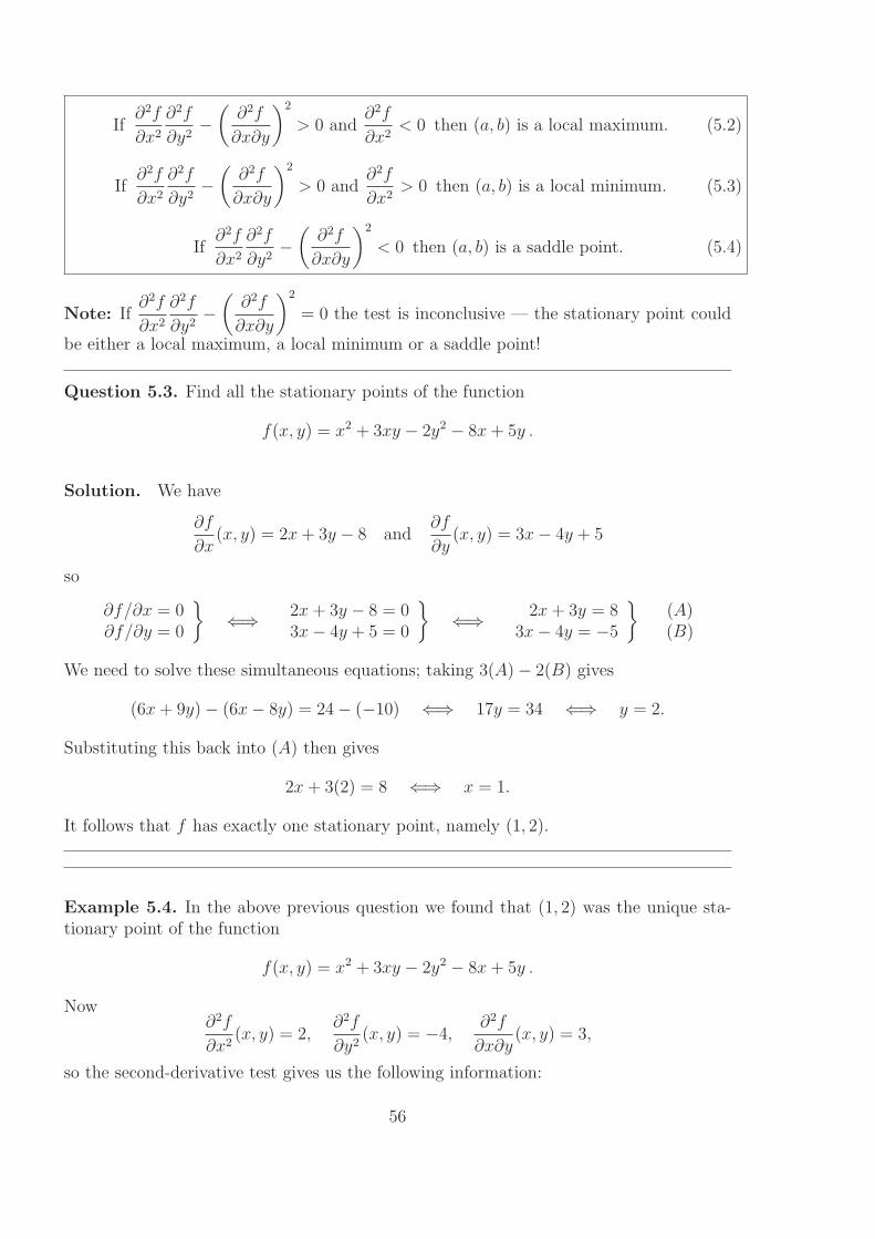
If∂2f
∂x2
∂2f
∂y2−
(∂2f
∂x∂y
)2
> 0 and∂2f
∂x2< 0 then (a, b) is a local maximum. (5.2)
If∂2f
∂x2
∂2f
∂y2−
(∂2f
∂x∂y
)2
> 0 and∂2f
∂x2> 0 then (a, b) is a local minimum. (5.3)
If∂2f
∂x2
∂2f
∂y2−
(∂2f
∂x∂y
)2
< 0 then (a, b) is a saddle point. (5.4)
Note: If∂2f
∂x2
∂2f
∂y2−
(∂2f
∂x∂y
)2
= 0 the test is inconclusive — the stationary point could
be either a local maximum, a local minimum or a saddle point!
Question 5.3. Find all the stationary points of the function
f(x, y) = x2 + 3xy − 2y2 − 8x+ 5y .
Solution. We have
∂f
∂x(x, y) = 2x+ 3y − 8 and
∂f
∂y(x, y) = 3x− 4y + 5
so
∂f/∂x = 0∂f/∂y = 0
}
⇐⇒ 2x+ 3y − 8 = 03x− 4y + 5 = 0
}
⇐⇒ 2x+ 3y = 83x− 4y = −5
}(A)(B)
We need to solve these simultaneous equations; taking 3(A)− 2(B) gives
(6x+ 9y)− (6x− 8y) = 24− (−10) ⇐⇒ 17y = 34 ⇐⇒ y = 2.
Substituting this back into (A) then gives
2x+ 3(2) = 8 ⇐⇒ x = 1.
It follows that f has exactly one stationary point, namely (1, 2).
Example 5.4. In the above previous question we found that (1, 2) was the unique sta-tionary point of the function
f(x, y) = x2 + 3xy − 2y2 − 8x+ 5y .
Now∂2f
∂x2(x, y) = 2,
∂2f
∂y2(x, y) = −4,
∂2f
∂x∂y(x, y) = 3,
so the second-derivative test gives us the following information:
56

Stationary point∂2f
∂x2
∂2f
∂x∂y
∂2f
∂y2∂2f
∂x2
∂2f
∂y2− (
∂2f
∂x∂y)2 Nature of stationary point
(1, 2) 2 3 −4 −17 < 0 saddle point
Question 5.4. Find and classify all the stationary points of the function
f(x, y) = xy(1− x− y).
Solution. We have
∂f
∂x(x, y) = −xy + y(1− x− y) = y(1− 2x− y)
and∂f
∂y(x, y) = −xy + x(1− x− y) = x(1− x− 2y) .
Therefore∂f∂x(x, y) = 0
∂f∂y(x, y) = 0
}
⇐⇒ y(1− 2x− y) = 0x(1− x− 2y) = 0
}
We must solve these simultaneous equations; this can be done by considering four separatecases:
Case (i):y = 0x = 0
}
This immediately gives the stationary point (0, 0).
Case (ii):y = 0
1− x− 2y = 0
}
Putting y = 0 in the second equation gives 1 − x − 0 = 0 or x = 1. Thus we get thestationary point (1, 0).
Case (iii):1− 2x− y = 0
x = 0
}
Putting x = 0 in the first equation gives 1−0−y = 0 or y = 1. Thus we get the stationarypoint (0, 1).
Case (iv):1− 2x− y = 01− x− 2y = 0
}
⇐⇒ 2x+ y = 1x+ 2y = 1
}(A)(B)
Taking (A)− 2(B) gives
(2x+ y)− (2x+ 4y) = 1− 2 ⇐⇒ −3y = −1 ⇐⇒ y = 13.
57
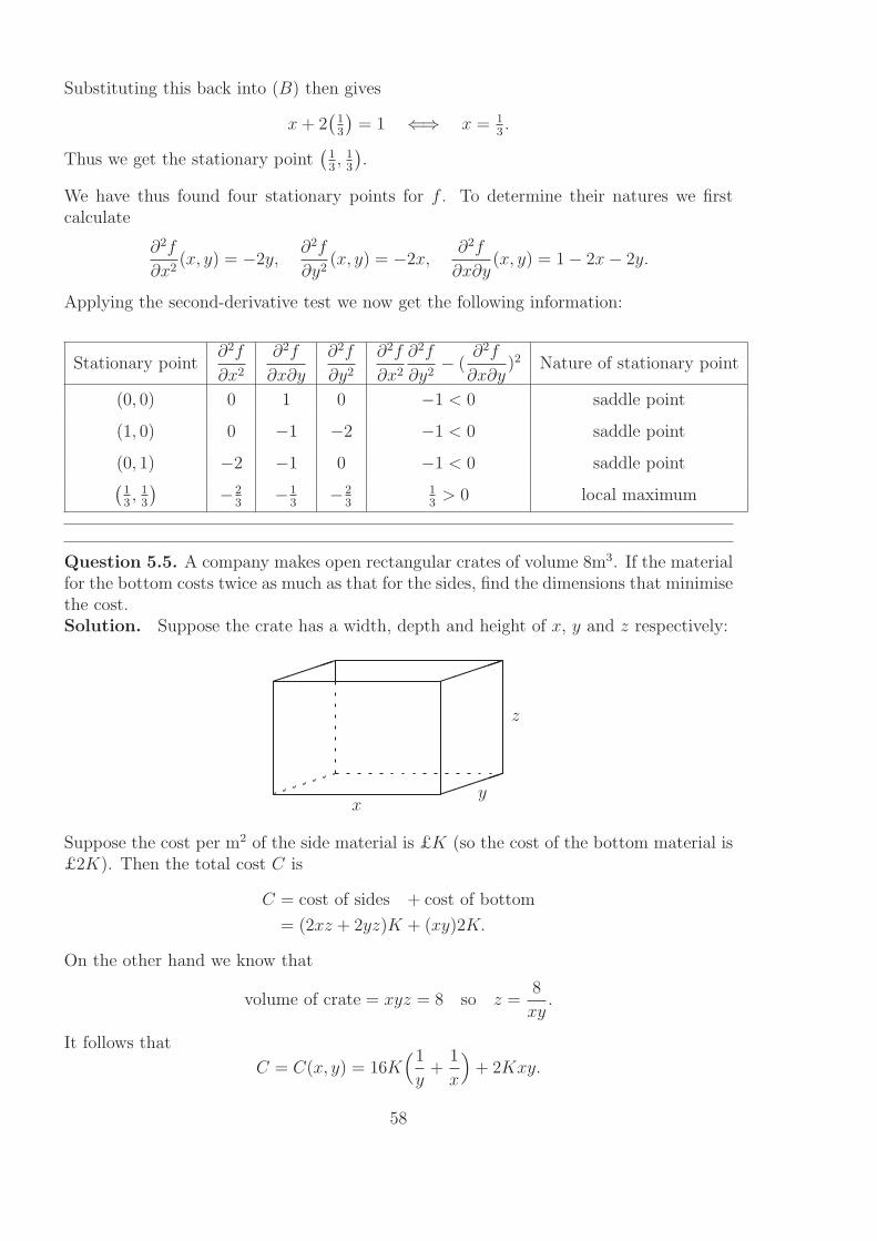
Substituting this back into (B) then gives
x+ 2(13
)= 1 ⇐⇒ x = 1
3.
Thus we get the stationary point(13, 13
).
We have thus found four stationary points for f . To determine their natures we firstcalculate
∂2f
∂x2(x, y) = −2y,
∂2f
∂y2(x, y) = −2x,
∂2f
∂x∂y(x, y) = 1− 2x− 2y.
Applying the second-derivative test we now get the following information:
Stationary point∂2f
∂x2
∂2f
∂x∂y
∂2f
∂y2∂2f
∂x2
∂2f
∂y2− (
∂2f
∂x∂y)2 Nature of stationary point
(0, 0) 0 1 0 −1 < 0 saddle point
(1, 0) 0 −1 −2 −1 < 0 saddle point
(0, 1) −2 −1 0 −1 < 0 saddle point(13, 13
)−2
3−1
3−2
313> 0 local maximum
Question 5.5. A company makes open rectangular crates of volume 8m3. If the materialfor the bottom costs twice as much as that for the sides, find the dimensions that minimisethe cost.Solution. Suppose the crate has a width, depth and height of x, y and z respectively:
✏✏✏✏✏✏✏✏✏✏
✏✏✏✏✏
xy
z
Suppose the cost per m2 of the side material is £K (so the cost of the bottom material is£2K). Then the total cost C is
C = cost of sides + cost of bottom
= (2xz + 2yz)K + (xy)2K.
On the other hand we know that
volume of crate = xyz = 8 so z =8
xy.
It follows that
C = C(x, y) = 16K(1
y+
1
x
)
+ 2Kxy.
58

We now find the stationary points of C; firstly we calculate
∂C
∂x(x, y) = −16K
x2+ 2Ky and
∂C
∂y(x, y) = −16K
y2+ 2Kx.
The stationary points are then given by solving
∂C
∂x(x, y) = 0
∂C
∂y(x, y) = 0
⇐⇒−16K
x2+ 2Ky = 0
−16K
y2+ 2Kx = 0
⇐⇒y =
8
x2
x =8
y2
(A)
(B)
Substituting (A) into (B) gives
x =8
(8x2
)2 ⇐⇒ x =x4
8⇐⇒ x3 = 8 ⇐⇒ x = 2.
Substituting this back into (A) then gives
y =8
22= 2.
Thus C(x, y) has the stationary point (2, 2). We can use the second derivative test tocheck that this stationary point is a minimum for the cost; alternatively this point is quiteclear if one thinks about the set up of the problem.Finally we note that when x = y = 2 we have z = 8/(xy) = 2 so the cheapest shape tomake the crate is as a cube measuring 2m×2m×2m.
59
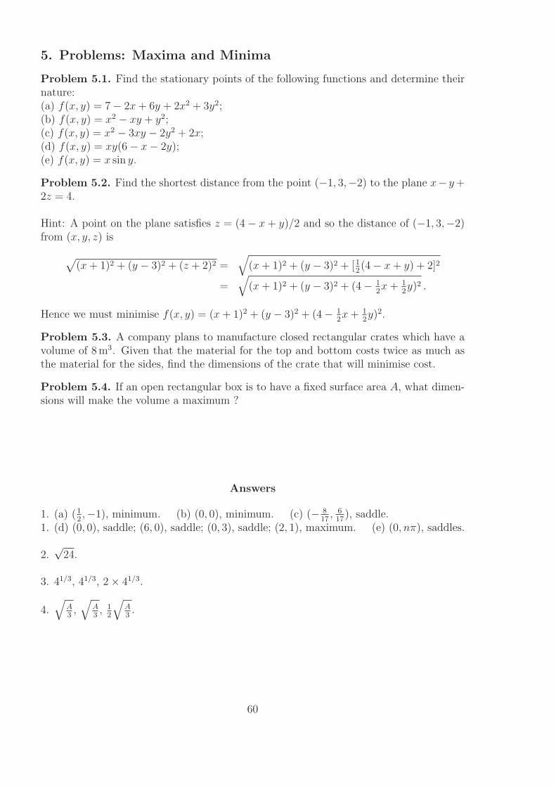
5. Problems: Maxima and Minima
Problem 5.1. Find the stationary points of the following functions and determine theirnature:(a) f(x, y) = 7− 2x+ 6y + 2x2 + 3y2;(b) f(x, y) = x2 − xy + y2;(c) f(x, y) = x2 − 3xy − 2y2 + 2x;(d) f(x, y) = xy(6− x− 2y);(e) f(x, y) = x sin y.
Problem 5.2. Find the shortest distance from the point (−1, 3,−2) to the plane x− y+2z = 4.
Hint: A point on the plane satisfies z = (4− x + y)/2 and so the distance of (−1, 3,−2)from (x, y, z) is
√
(x+ 1)2 + (y − 3)2 + (z + 2)2 =√
(x+ 1)2 + (y − 3)2 + [12(4− x+ y) + 2]2
=√
(x+ 1)2 + (y − 3)2 + (4− 12x+ 1
2y)2 .
Hence we must minimise f(x, y) = (x+ 1)2 + (y − 3)2 + (4− 12x+ 1
2y)2.
Problem 5.3. A company plans to manufacture closed rectangular crates which have avolume of 8m3. Given that the material for the top and bottom costs twice as much asthe material for the sides, find the dimensions of the crate that will minimise cost.
Problem 5.4. If an open rectangular box is to have a fixed surface area A, what dimen-sions will make the volume a maximum ?
Answers
1. (a) (12,−1), minimum. (b) (0, 0), minimum. (c) (− 8
17, 617), saddle.
1. (d) (0, 0), saddle; (6, 0), saddle; (0, 3), saddle; (2, 1), maximum. (e) (0, nπ), saddles.
2.√24.
3. 41/3, 41/3, 2× 41/3.
4.√
A3,√
A3, 1
2
√A3.
60

Chapter 6
Taylor Series and LinearApproximation
Recall, first, what happens for a function of only one variable.
Example 6.1. If h is small then h2 and h3 etc., are very small compared to h. Forexample, if
h = 0.02 then h2 = 0.0004.
A function f(x) with x “near” some value a, say x = a + h, can then be given by itsTaylor series:
f(x) = f(a+ h) = f(a) + hdf
dx(a) +
h
2
d2f
dx2(a) + . . . .
With h small enough we might stop with the second term on the right-hand side to getthe linear approximation
f(x) = f(a+ h) ≈ f(a) + hdf
dx(a) .
Question 6.1. Use linear approximation to estimate (1.01)1/3.Solution. Take f(x) = x1/3 so f ′(x) = 1
3x−2/3. Then
(1.01)1/3 = f(1 + 0.01)
≈ f(1) + f ′(1)× 0.01
= 1 +1
3× 0.01
≈ 1.0033.
Linear approximation replaces the graph of f with a section of straight line.
61
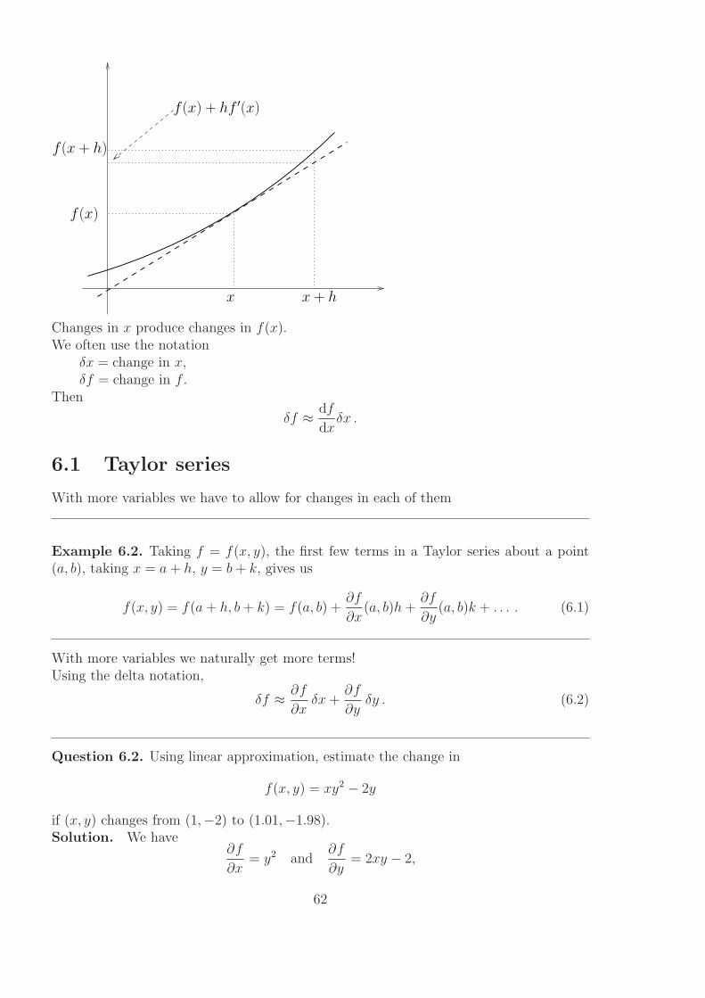
x x + h
f (x) + hf ′(x)
f (x)
f (x + h)
Changes in x produce changes in f(x).We often use the notation
δx = change in x,δf = change in f .
Then
δf ≈ df
dxδx .
6.1 Taylor series
With more variables we have to allow for changes in each of them
Example 6.2. Taking f = f(x, y), the first few terms in a Taylor series about a point(a, b), taking x = a+ h, y = b+ k, gives us
f(x, y) = f(a+ h, b+ k) = f(a, b) +∂f
∂x(a, b)h+
∂f
∂y(a, b)k + . . . . (6.1)
With more variables we naturally get more terms!Using the delta notation,
δf ≈ ∂f
∂xδx+
∂f
∂yδy . (6.2)
Question 6.2. Using linear approximation, estimate the change in
f(x, y) = xy2 − 2y
if (x, y) changes from (1,−2) to (1.01,−1.98).Solution. We have
∂f
∂x= y2 and
∂f
∂y= 2xy − 2,
62
while
δx = 1.01− 1 = 0.01 and δy = −1.98− (−2) = 0.02.
Therefore
δf ≈ ∂f
∂x(1,−2)× δx+
∂f
∂y(1,−2)× δy
= 4× 0.01 + (−6)× 0.02
= −0.08.
Question 6.3. Using linear approximation, estimate the change in
f(x, y) = xy3
if (x, y) changes from (1, 2) to (0.99, 2.02).Solution. We have
∂f
∂x= y3 and
∂f
∂y= 3xy2,
while
δx = 0.99− 1 = −0.01 and δy = 2.02− 2 = 0.02.
Therefore
δf ≈ ∂f
∂x(1, 2)× δx+
∂f
∂y(1, 2)× δy = 8× (−0.01) + 12× 0.02 = 0.16 .
6.2 Estimation of errors
We can use linear approximation to estimate the effect of errors in measurements:
• Suppose that we are interested in a quantity Q(x, y).
• We make measurements of x and y with errors δx and δy.
• The corresponding error in Q is
δQ ≈ ∂Q
∂xδx+
∂Q
∂yδy.
Example 6.3. A company makes tanks 6m high with a of radius 2m. How do errors inconstruction affect the volume? Consider a tank of height h and radius r:
63
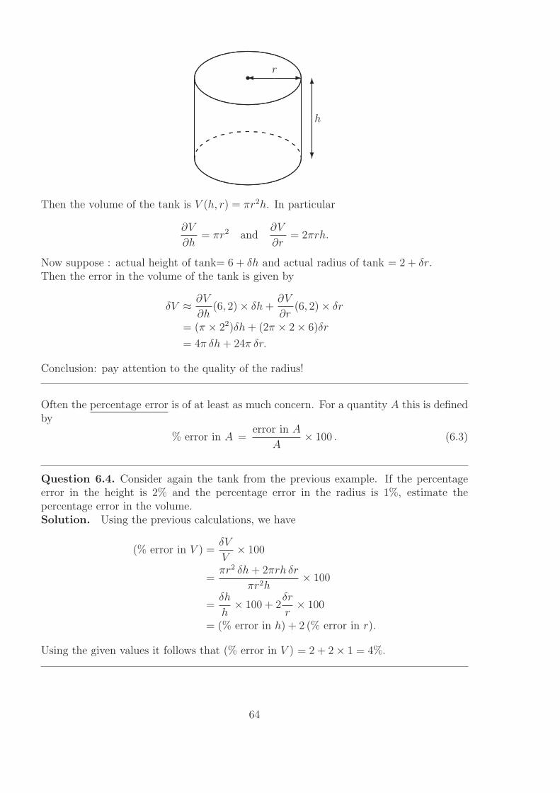
....................................................
..................................
................................................................................................................................................................................................................................................................................................................................................................................. ............. .............. ................ .................. ................... ..................... ...................... ................................. .................................. .................................. ................................. ...................... .....................
.........................................................................................................
.......................... ............. .............. ................ .................. ................... ..................... ...................... ................................. .................................. .................................. ................................. ...................... .................................................................................................................................................
.........................
.......................................................................................................................................................
s ✲✛ r
✻
❄
h
Then the volume of the tank is V (h, r) = πr2h. In particular
∂V
∂h= πr2 and
∂V
∂r= 2πrh.
Now suppose : actual height of tank= 6 + δh and actual radius of tank = 2 + δr.Then the error in the volume of the tank is given by
δV ≈ ∂V
∂h(6, 2)× δh+
∂V
∂r(6, 2)× δr
= (π × 22)δh+ (2π × 2× 6)δr
= 4π δh+ 24π δr.
Conclusion: pay attention to the quality of the radius!
Often the percentage error is of at least as much concern. For a quantity A this is definedby
% error in A =error in A
A× 100 . (6.3)
Question 6.4. Consider again the tank from the previous example. If the percentageerror in the height is 2% and the percentage error in the radius is 1%, estimate thepercentage error in the volume.Solution. Using the previous calculations, we have
(% error in V ) =δV
V× 100
=πr2 δh+ 2πrh δr
πr2h× 100
=δh
h× 100 + 2
δr
r× 100
= (% error in h) + 2 (% error in r).
Using the given values it follows that (% error in V ) = 2 + 2× 1 = 4%.
64

Question 6.5. A company makes boxes with dimensions x, y and z.
✏✏✏✏✏✏✏✏✏✏
✏✏✏✏✏
xy
z
Estimate the percentage error in the volume in terms of the percentage errors in x, y andz.Solution. The volume of the box is given as V (x, y, z) = xyz so
δV ≈ ∂V
∂xδx+
∂V
∂yδy +
∂V
∂zδz
= yz δx+ xz δy + xy δz.
HenceδV
V≈ yz δx
xyz+
xz δy
xyz+
xy δz
xyz=
δx
x+
δy
y+
δz
z.
It follows that
(% error in V ) =δV
V× 100
≈ δx
x× 100 +
δy
y× 100 +
δz
z× 100
= (% error in x) + (% error in y) + (% error in z).
65
6. Problems: Linear Approximation and Error Analysis
Problem 6.1. Consider the function f(x) = x1/3.
Derive a linear approximation (using Taylor series) centred at x0 = 8. Use the linearapproximation to approximate 91/3.
What is the percentage error in the approximation compared to the true value of 91/3.
Problem 6.2. Use linear approximation to estimate√24.
Problem 6.3. Use linear approximation to estimate the change in f(x, y) = x2 − 3x3y+4x− 2y3+6 if (x, y) changes from (−2, 3) to (−2.02, 3.01) and hence find an approximatevalue for f(−2.02, 3.01).
Problem 6.4. The dimensions of a closed rectangular box are measured as 3 m, 4 m,and 5m with maximum possible error of 0.1 cm. Using linear approximation find themaximum error in the calculated values of (i) the volume of the box, and (ii) the surfacearea of the box.
Problem 6.5. The height of a tower is calculated by measuring the horizontal distancex from the foot of the tower to a point A and the angle of elevation θ of the top of thetower from A. Using linear approximation, estimate the percentage error in the height interms of the percentage errors in x and θ.
Problem 6.6. The rate of flow of gas in a pipe is given by v = Cd1
2T− 5
6 where C is aconstant, d is the diameter of the pipe and T is the temperature of the gas. By usinglinear approximation, find the % change in v when the diameter of the pipe is increasedby 1% and the gas temperature is increased by 2%.
Answers
1. f(x) ≈ 2 + 112(x− 8), 91/3 ≈ 2.0833, 0.16% .
2. 4.9.
3. 1.86, 21.86.
4. 0.047 m3, 0.048 m2.
5. % error in x+θ
sin θ cos θ× % error in θ.
6. −76% .
66

Chapter 7
Multiple Integrals
7.1 Integration of functions of one variable
We start by recalling the basics of integration with respect to a single variable.We have results such as:
∫ b
a
f(x) dx =[F (x)
]b
a:= F (b)−F (a)
where F is an “antiderivative” or indefinite integral of f . (f = dF/dx.)
∫
λf(x) dx = λ
∫
f(x) dx,
∫
(f(x) + g(x)) dx =
∫
f(x) dx+
∫
g(x) dx .
Useful techniques include:
• Integration by parts.
• Integration by substitution.
• Use of partial fractions.
Some specific integrals can be found on the formula sheet.
Question 7.1. Calculate
∫ 1
0
(3x4 + x2ex
3)dx.
Solution. This integral is designed to use a few different techniques! Firstly we cansplit the integral as
∫ 1
0
(3x4 + x2ex
3)dx = 3
∫ 1
0
x4 dx+
∫ 1
0
x2ex3
dx.
The first integral on the right-hand side is straightforward:
∫ 1
0
x4 dx =[x5
5
]1
0=
1
5.
67
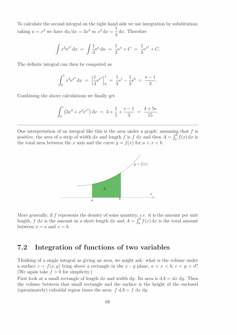
To calculate the second integral on the right hand side we use integration by substitution;
taking u = x3 we have du/dx = 3x2 so x2 dx =1
3du. Therefore
∫
x2ex3
dx =
∫1
3eu du =
1
3eu + C =
1
3ex
3
+ C.
The definite integral can then be computed as
∫ 1
0
x2ex3
dx =[1
3ex
3
]1
0=
1
3e1 − 1
3e0 =
e− 1
3.
Combining the above calculations we finally get
∫ 1
0
(3x4 + x2ex
3)dx = 3× 1
5+
e− 1
3=
4 + 5e
15.
One interpretation of an integral like this is the area under a graph: assuming that f ispositive, the area of a strip of width dx and length f is f dx and then A =
∫ b
af(x) dx is
the total area between the x axis and the curve y = f(x) for a < x < b.
y = f (x)
x
a b
A
More generally, if f represents the density of some quantity, i.e. it is the amount per unitlength, f dx is the amount in a short length dx and A =
∫ b
af(x) dx is the total amount
between x = a and x = b.
7.2 Integration of functions of two variables
Thinking of a single integral as giving an area, we might ask: what is the volume undera surface z = f(x, y) lying above a rectangle in the x - y plane, a < x < b, c < y < d?(We again take f > 0 for simplicity.)
First look at a small rectangle of length dx and width dy. Its area is dA = dx dy. Thenthe volume between that small rectangle and the surface is the height of the enclosed(aproximately) cuboidal region times the area: f dA = f dx dy.
68

dydx
z = f (x, y)
f
The volume between the x - y plane and the surface in the slab of width dx between y = cand y = d is then given by integrating with respect to y: (
∫ d
cf(x, y) dy) dx. (In doing this
integral, x is held fixed.) Finally, to get the total volume, we must integrate with respectto x from a to b:
volume = V =
∫ b
a
(∫ d
c
f(x, y) dy
)
dx . (7.1)
We usually abbreviate this double integral as
V =
∫ b
a
∫ d
c
f(x, y) dy dx . (7.2)
Noting that, for cases we’ll be considering at least, we could have integrated with respectto x first and then y, we also have
V =
∫ d
c
∫ b
a
f(x, y) dx dy =
∫ ∫
D
f(x, y) dx dy , (7.3)
where D is our region of integration, here D is the rectangle a < x < b, c < y < d.More generally if f once again represents some sort of density, e.g. mass per unit area ina sheet of metal, the double integral
∫ ∫
Df(x, y) dx dy is the total amount in the region
D.
Example 7.1. An example of a double integral is
∫ 4
1
∫ −1
−3
(x2y + sin(xy)
)dy dx.
Question 7.2. Calculate
∫ 4
2
∫ 3
1
(xy2 + y) dy dx.
Solution. Calculating the inner integral first gives
∫ 3
1
(xy2 + y) dy =
[xy3
3+
y2
2
]3
1
=(
9x+9
2
)
−(x
3+
1
2
)
=26x
3+ 4 .
69

Therefore ∫ 4
2
∫ 3
1
(xy2 + y) dy dx =
∫ 4
2
(26x
3+ 4
)
dx
=
[13x2
3+ 4x
]4
2
=(13× 16
3+ 16
)
−(13× 4
3+ 8
)
= 13× 4 + 8 = 60 .
Question 7.3. Calculate
∫ 1
0
∫ 3
2
2xy dx dy.
Solution. Calculating the inner integral first gives
∫ 3
2
2xy dx =[x2y
]3
2= 9y − 4y = 5y.
Therefore∫ 1
0
∫ 3
2
2xy dx dy =
∫ 1
0
5y dy =
[5y2
2
]1
0
=5
2.
Example 7.2. For the double integral
∫ 3
2
∫ 1
0
2xyexy2
dy dx the region of integration D is
the rectangle given by0 ≤ y ≤ 1, 2 ≤ x ≤ 3.
✲x
✻y
D
2 3
1
Question 7.4. Calculate
∫ 3
2
∫ 1
0
2xyexy2
dy dx.
Solution. Firstly consider the inner integral
∫ 1
0
2xyexy2
dy.
We will use integration by substitution for this integral; taking u = xy2 we have∂u
∂y= 2xy
so du = 2xy dy and hence∫
2xyexy2
dy =
∫
eu du = eu + C = exy2
+ C.
70

Thus ∫ 1
0
2xyexy2
dy =[exy
2]1
0= ex − 1.
It follows that∫ 3
2
∫ 1
0
2xyexy2
dy dx =
∫ 3
2
(ex − 1) dx =[ex − x
]3
2= (e3 − 3)− (e2 − 2) = e3 − e2 − 1 .
Question 7.5. Let D be the rectangle given by
−1 ≤ y ≤ 0, 1 ≤ x ≤ 3.
Calculate
∫∫
D
(x2 + y) dy dx.
Solution. The region of integration is the following:
✲x
✻y
D
1 3
−1
Now∫∫
D
(x2 + y) dy dx =
∫ 3
1
∫ 0
−1
(x2 + y) dy dx =
∫ 3
1
[
x2y +y2
2
]0
−1
dx =
∫ 3
1
(
x2 − 1
2
)
dx
=
[x3
3− x
2
]3
1
=(
9− 3
2
)
−(1
3− 1
2
)
=23
3.
Of course a region of integration need not be rectangular. If D can be described byg(x) < y < h(x) for a < x < b, the (double) integral of f(x, y) over D will be
∫ ∫
D
f(x, y) dy dx =
∫ b
a
(∫ h(x)
g(x)
f(x, y) dy
)
dx .
We can drop the brackets and simply write this as∫ b
a
∫ h(x)
g(x)f(x, y) dy dx.
Example 7.3. Consider the region given by
−1
2≤ x ≤ 1
2, −
√1− x2 ≤ y ≤
√1− x2.
This region is part of a disc.
71

✲x
✻y
−1 1
y =√1− x2
✂✂✌
y = −√1− x2
❇❇▼
Example 7.4. Consider the region D:
✲x
✻y
D
1
1
y = 1− x!!✠
In this region we have 0 ≤ x ≤ 1 whilst, for a given x, 0 ≤ y ≤ 1− x. Thus the region Dis described by
0 ≤ x ≤ 1, 0 ≤ y ≤ 1− x.
Question 7.6. Calculate
∫ ∫
D
y dA over the region D below:
Solution. In this region we have 0 ≤ x ≤ 1, whilst, for a given x, we have
√x ≤ y ≤ 1.
0
1
1
y =√x
x
y
D
72

Therefore ∫ ∫
D
y dA =
∫ 1
0
∫ 1
√x
y dy dx.
Calculating the inner integral first gives
∫ 1
√x
y dy =[y2
2
]1
√x=
1
2− x
2.
Hence∫
D
y dA =
∫ 1
0
(1
2− x
2
)
dx =
[x
2− x2
4
]1
0
= 0−(1
2− 1
4
)
=1
4.
Example 7.5. Consider the region D:
✲x
✻y
D
1
1
y = x ❍❍❥
In this region we have 0 ≤ y ≤ 1, whilst, for a given y, y ≤ x ≤ 1.
Question 7.7. Calculate
∫∫
D
(3 − x − y) dA where D is the region described in the
previous question.Solution. Recall that D is described by
0 ≤ y ≤ 1, y ≤ x ≤ 1.
Therefore ∫∫
(3− x− y) dA =
∫ 1
0
∫ 1
y
(3− x− y) dx dy.
Now
∫ 1
y
(3− x− y) dx =
[
3x− x2
2− yx
]1
y
=(
3− 1
2− y
)
−(
3y − y2
2− y2
)
=5
2− 4y +
3y2
2.
It follows that
∫∫
(3− x− y) dA =
∫ 1
0
(5
2− 4y+
3y2
2
)
dy =
[5y
2− 2y2 +
y3
2
]1
0
=(5
2− 2 +
1
2
)
− 0 = 1 .
73
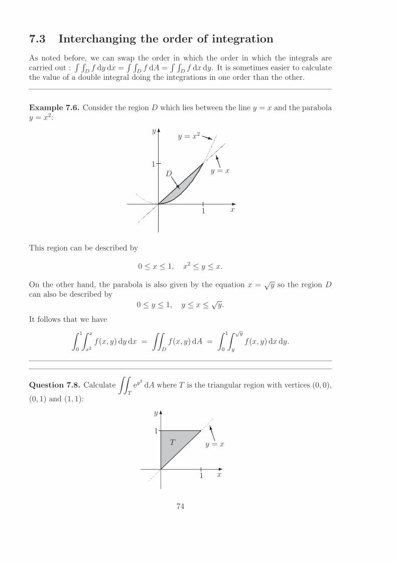
7.3 Interchanging the order of integration
As noted before, we can swap the order in which the order in which the integrals arecarried out :
∫ ∫
Df dy dx =
∫ ∫
Df dA =
∫ ∫
Df dx dy. It is sometimes easier to calculate
the value of a double integral doing the integrations in one order than the other.
Example 7.6. Consider the region D which lies between the line y = x and the parabolay = x2:
✲x
✻y
D❏❏❫
1
1
y = x2 PPq
y = x❇❇▼
This region can be described by
0 ≤ x ≤ 1, x2 ≤ y ≤ x.
On the other hand, the parabola is also given by the equation x =√y so the region D
can also be described by
0 ≤ y ≤ 1, y ≤ x ≤ √y.
It follows that we have
∫ 1
0
∫ x
x2
f(x, y) dy dx =
∫∫
D
f(x, y) dA =
∫ 1
0
∫ √y
y
f(x, y) dx dy.
Question 7.8. Calculate
∫∫
T
ey2
dA where T is the triangular region with vertices (0, 0),
(0, 1) and (1, 1):
✲x
✻y
T
1
1
y = x❇❇❇▼
74

Solution. As a first attempt we may describe T by
0 ≤ x ≤ 1, x ≤ y ≤ 1.
It follows that ∫∫
T
ey2
dA =
∫ 1
0
∫ 1
x
ey2
dy dx.
The inner integral is then∫ 1
x
ey2
dy
which can’t be evaluated very easily! We’ve got stuck!
As a second attempt let us describe T the other way; that is
0 ≤ y ≤ 1, 0 ≤ x ≤ y.
Then ∫∫
T
ey2
dA =
∫ 1
0
∫ y
0
ey2
dx dy.
Evaluating the inner integral first gives
∫ y
0
ey2
dx =[xey
2]y
0= yey
2
.
It follows that
∫∫
T
ey2
dA =
∫
yey2
dy =[ey
2
2
]1
0=
e
2− 1
2=
1
2(e− 1) ,
where we used the substitution u = y2 to evaluate the integral.
Note. On evaluating a double integral I =∫ ∫
Df(x, y) dA by doing the y integral first,
i.e. taking I =∫ b
a
∫ g2(x)
g1(x)f(x, y) dy dx, we integrate along vertical strips between the lower
boundary, say y = g1(x), and the upper boundary, say y = g2(x) (this gives a result which
generally depends upon x, but definitely does not depend on y): Iy(x) =∫ g2(x)
g1(x)f(x, y) dy.
We then total up the contributions of strips by integrating Iy from the lowest value
of x taken in D, say a, to the largest, say b (see Fig. 7.1(i)): I =∫ b
af(x, y) dx. On
the other hand, doing the y integral first, we take I =∫ d
c
∫ h2(y)
h1(y)f(x, y) dx dy, we integrate
along horizontal strips between the left-hand boundary, say x = h1(y), and the right-handboundary, say x = h2(y) (this gives a result which generally depends upon y, but definitely
does not depend on x): Ix(y) =∫ h2(y)
h1(y)f(x, y) dx. We then total up the contributions of
strips by integrating Ix from the lowest value of y taken in D, say c, to the largest, say d(see Fig. 7.1(ii)). (Either way, the final result does not depend on either x or y!)
75

(i) (ii)
DD
xba
y y
x
c
d
y = g1(x)
y = g2(x)
x = h2(y)
x = h2(y)
Figure 7.1: Different orders of integration over D.
76
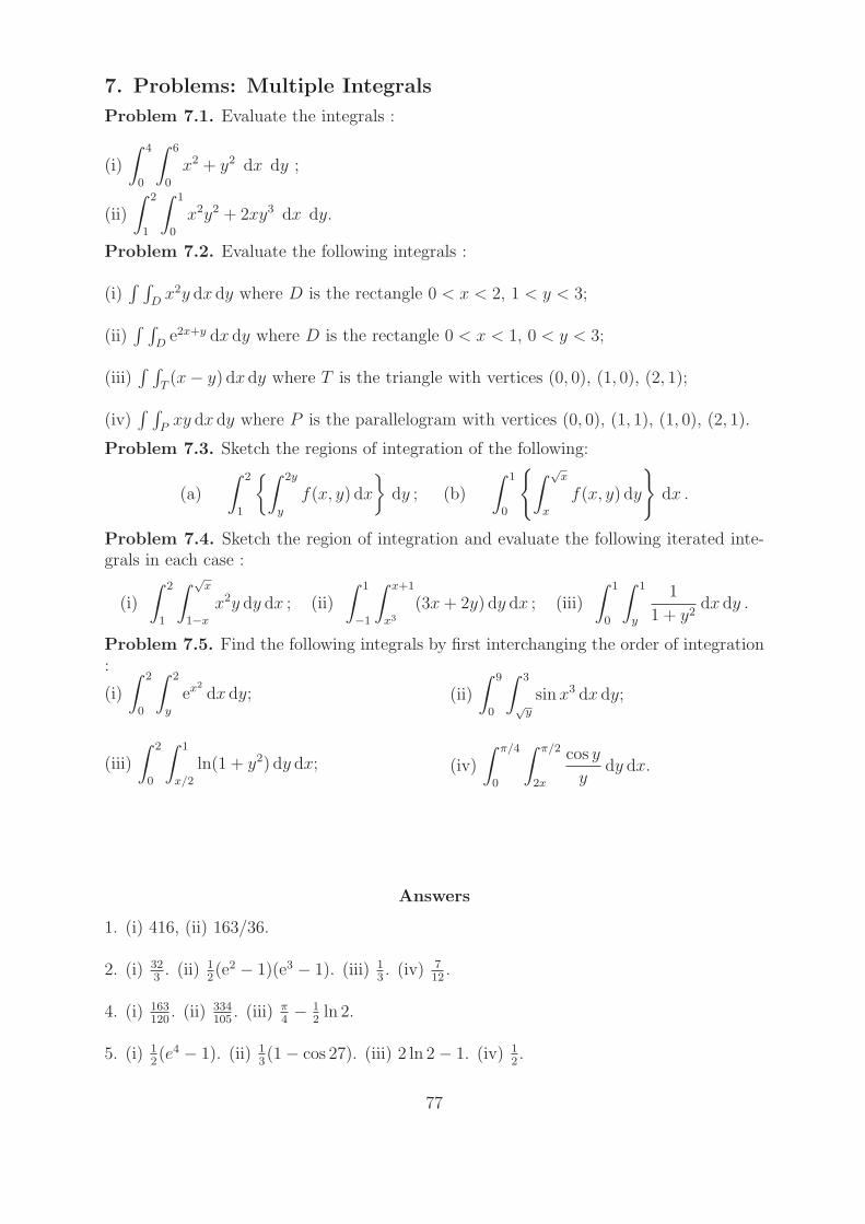
7. Problems: Multiple Integrals
Problem 7.1. Evaluate the integrals :
(i)
∫ 4
0
∫ 6
0
x2 + y2 dx dy ;
(ii)
∫ 2
1
∫ 1
0
x2y2 + 2xy3 dx dy.
Problem 7.2. Evaluate the following integrals :
(i)∫ ∫
Dx2y dx dy where D is the rectangle 0 < x < 2, 1 < y < 3;
(ii)∫ ∫
De2x+y dx dy where D is the rectangle 0 < x < 1, 0 < y < 3;
(iii)∫ ∫
T(x− y) dx dy where T is the triangle with vertices (0, 0), (1, 0), (2, 1);
(iv)∫ ∫
Pxy dx dy where P is the parallelogram with vertices (0, 0), (1, 1), (1, 0), (2, 1).
Problem 7.3. Sketch the regions of integration of the following:
(a)
∫ 2
1
{∫ 2y
y
f(x, y) dx
}
dy ; (b)
∫ 1
0
{∫ √
x
x
f(x, y) dy
}
dx .
Problem 7.4. Sketch the region of integration and evaluate the following iterated inte-grals in each case :
(i)
∫ 2
1
∫ √x
1−x
x2y dy dx ; (ii)
∫ 1
−1
∫ x+1
x3
(3x+ 2y) dy dx ; (iii)
∫ 1
0
∫ 1
y
1
1 + y2dx dy .
Problem 7.5. Find the following integrals by first interchanging the order of integration:
(i)
∫ 2
0
∫ 2
y
ex2
dx dy;
(iii)
∫ 2
0
∫ 1
x/2
ln(1 + y2) dy dx;
(ii)
∫ 9
0
∫ 3
√y
sin x3 dx dy;
(iv)
∫ π/4
0
∫ π/2
2x
cos y
ydy dx.
Answers
1. (i) 416, (ii) 163/36.
2. (i) 323. (ii) 1
2(e2 − 1)(e3 − 1). (iii) 1
3. (iv) 7
12.
4. (i) 163120
. (ii) 334105
. (iii) π4− 1
2ln 2.
5. (i) 12(e4 − 1). (ii) 1
3(1− cos 27). (iii) 2 ln 2− 1. (iv) 1
2.
77

78

Chapter 8
Double Integrals: Applications andPolar Coordinates
8.1 Change of variables to polar coordinates
We must first be familiar with polar coordinates.
Question 8.1. Convert the function
f(x, y) =2xy
x2 + y2.
into a function of polar coordinates.Solution. We need to make the substitutions
x = r cos θ , y = r sin θ .
This gives us
f(r, θ) =2 r cos θ × r sin θ
r2 cos2 θ + r2 sin2 θ=
r2 2 cos θ sin θ
r2(cos2 θ + sin2 θ)= sin 2θ .
Now we can look at how they are used for double integrals.A key step is to see what replaces the dx dy we were using for Cartesian co-ordinates wehad our small area element a rectangle of area dA = dx dy. For polars, with change inangle, dθ, and change in distance from the origin, dr, both small, we get something whichis approximately rectangular, with sides of length rdθ and dr.
r
dθ
r dθdr
dA
79

We can then write a double integral∫ ∫
f dA =∫ ∫
f dx dy as∫ ∫
f dA =∫ ∫
fr dr dθ.
Example 8.1. The quarter circle
✲
✻
2
2
is given by
0 ≤ r ≤ 2, 0 ≤ θ ≤ π
2,
whilst the annulus
✲
✻
1 2
is given by1 ≤ r ≤ 2, 0 ≤ θ ≤ 2π.
Question 8.2. Calculate
∫ 1
0
∫ √1−x2
0
5√
x2 + y2 dy dx .
Solution. Clearly this is going to be very messy if we use cartesian coordinates. Onthe other hand, converting the integrand to polar coordinates gives
5√
x2 + y2 = 5√
r2 cos2 θ + r2 sin2 θ = 5r,
whilst the region of integration
0 ≤ x ≤ 1, 0 ≤ y ≤√1− x2
is a quarter circle (n.b. if y =√1− x2 then x2 + y2 = 1 which is the equation for the
circle of radius 1, centred at the origin):
80

✲
✻
1
1y =
√1− x2
!!✠
Thus, in polar coordinates, the region of integration is given by
0 ≤ r ≤ 1, 0 ≤ θ ≤ π
2.
It follows that∫ 1
0
∫ √1−x2
0
5√
x2 + y2 dy dx =
∫ π/2
0
∫ 1
0
5r r dr dθ.
Calculating the inner integral gives
∫ 1
0
5r2 dr =[5r3
3
]1
0=
5
3.
Therefore∫ π/2
0
∫ 1
0
5r r dr dθ =
∫ π/2
0
5
3dθ =
[5θ
3
]π/2
0=
5π
6.
8.2 Volume
Question 8.3. Find the volume of the solid which lies under the graph of
f(x, y) = x2 + 3y2
over the triangle with corners (0, 0), (0, 1) and (1, 0).Solution. The region of integration is the following
✲x
✻y
1
1
y = 1− x!!✠
which can be defined by0 ≤ x ≤ 1, 0 ≤ y ≤ 1− x.
81

Therefore
Volume =
∫ 1
0
∫ 1−x
0
(x2 + 3y2) dy dx.
Calculating the inner integral first gives
∫ 1−x
0
(x2 + 3y2) dy =[x2y + y3
]1−x
0= x2(1− x) + (1− x)3.
Hence
Volume =
∫ 1
0
(x2−x3+(1−x)3
)dx =
[x3
3− x4
4− (1− x)4
4
]1
0
=(1
3−1
4−0
)
−(
0−0−1
4
)
=1
3.
8.3 Average values
Example 8.2. Consider a 3m×3m metal plate R. For convenience take the origin to bethe bottom left corner.
✲x
✻y
R
3
3
Suppose the temperature at the point (x, y) is given by
T (x, y) = 40 + 2x+ 2y.
Then we can calculate
Average temperature of R =1
Area of R
∫∫
R
(40+2x+2y) dA =1
9
∫ 3
0
∫ 3
0
(40+2x+2y) dy dx
=1
9
∫ 3
0
[40y+2xy+ y2
]3
0dx =
1
9
∫ 3
0
(129+6x) dx =1
9
[129x+3x2
]3
0=
1
9(378+27) = 46 .
8.4 Mass and centre of mass
Question 8.4. Find the centre of mass of a triangular metal plate P with vertices at(0, 0), (1, 0) and (0, 1), and which has uniform density given by ρ(x, y) = 1 g/cm2.
82
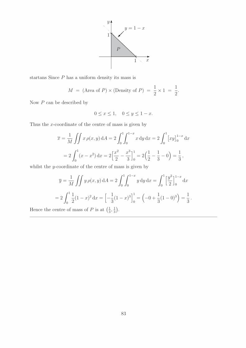
✲x
✻y
P
1
1
y = 1− x!!✠
startans Since P has a uniform density its mass is
M = (Area of P )× (Density of P ) =1
2× 1 =
1
2.
Now P can be described by
0 ≤ x ≤ 1, 0 ≤ y ≤ 1− x.
Thus the x-coordinate of the centre of mass is given by
x =1
M
∫∫
x ρ(x, y) dA = 2
∫ 1
0
∫ 1−x
0
x dy dx = 2
∫ 1
0
[xy
]1−x
0dx
= 2
∫ 1
0
(x− x2) dx = 2[x2
2− x3
3
]1
0= 2
(1
2− 1
3− 0
)
=1
3,
whilst the y-coordinate of the centre of mass is given by
y =1
M
∫∫
y ρ(x, y) dA = 2
∫ 1
0
∫ 1−x
0
y dy dx =
∫ 1
0
[y2
2
]1−x
0dx
= 2
∫ 1
0
1
2(1− x)2 dx =
[
−1
3(1− x)3
]1
0=
(
−0 +1
3(1− 0)3
)
=1
3.
Hence the centre of mass of P is at(13, 13
).
83
8. Problems: Applications of Multiple Integrals
Problem 8.1. Find∫ ∫
C
√
x2 + y2 dA where C is the circle x2 + y2 < a2.
Problem 8.2. For each of the following sketch the region of integration evaluate theintegral by using polar coordinates.
(a)
∫ 3
0
∫√
9−y2
0
x2y dx dy . (b)
∫ 1/√2
0
∫ √1−x2
x
√
1 + x2 + y2 dy dx .
Problem 8.3. Find∫ ∫
Dsin(
√
x2 + y2) dA where D is
(i) the semi-circle x2 + y2 < 1, y > 0;
(ii) the ring-shaped region 1 < x2 + y2 < 4.
Problem 8.4. Find the volume V of the solid bounded by the paraboloid z = 4−x2−y2
and the x - y plane.
Problem 8.5. Find the volume of the solid which lies under the surface z = x2+2y2 andover the triangle in the x - y plane with vertices (0, 0), (1, 0) and (1, 2).
Problem 8.6. Find the volume of the tetrahedron bounded by the co-ordinate planesand the plane of equation 2x+ y + z = 2.
Problem 8.7. A landscape is described by a function H(x, y) = x2 + y2 where x and yare co-ordinates on some map. This function gives the height above sea level at the point(x, y). Find the average height of the landscape above the rectangle 0 < x < 3, 1 < y < 2.
Problem 8.8. A flat plate in the shape of a triangle with vertices (0, 0), (1, 1), (2, 0)(using cm) lies in the x - y plane. The density of the plate, ρ(x, y), at the point (x, y) isequal to 1 + 6x + 12y g/cm2. Find the mass of the plate (given by
∫ ∫
Tρ(x, y) dx dy).
Write down the co-ordinates of the centre of mass of the triangle in terms of doubleintegrals.
84

Answers
1. 2πa3/3.
2. (a) 815. (b) π
12(2√2− 1).
3. (i) π(sin 1− cos 1). (ii) 2π(sin 2− 2 cos 2− sin 1 + sin 2).
4. 8π.
5. 116.
6. 23.
7. 163.
8. 11; 111
∫ 1
0
∫ 2−y
yx(1 + 6x+ 12y) dx dy; 1
11
∫ 1
0
∫ 2−y
yy(1 + 6x+ 12y) dx dy.
85