Math 6520: Differentiable Manifolds...
121
Math 6520: Differentiable Manifolds I Taught by Reyer Sjamaar Notes by David Mehrle [email protected] Cornell University Fall 2016 Last updated December 11, 2016. The latest version is online here.
Transcript of Math 6520: Differentiable Manifolds...

Math 6520: Differentiable Manifolds I
Taught by Reyer Sjamaar
Notes by David [email protected]
Cornell UniversityFall 2016
Last updated December 11, 2016.The latest version is online here.

Contents
1 Introduction . . . . . . . . . . . . . . . . . . . . . . . . . . . . . . . . . 51.1 Dimension . . . . . . . . . . . . . . . . . . . . . . . . . . . . . . . 91.2 Lots of Examples . . . . . . . . . . . . . . . . . . . . . . . . . . . 101.3 The Smooth Category . . . . . . . . . . . . . . . . . . . . . . . . . 14
2 Tangent Vectors . . . . . . . . . . . . . . . . . . . . . . . . . . . . . . . 152.1 Derivations . . . . . . . . . . . . . . . . . . . . . . . . . . . . . . . . 21
3 Submanifolds . . . . . . . . . . . . . . . . . . . . . . . . . . . . . . . . 263.1 Rank . . . . . . . . . . . . . . . . . . . . . . . . . . . . . . . . . . . 313.2 Submersions and Immersions . . . . . . . . . . . . . . . . . . . . 353.3 Embeddings . . . . . . . . . . . . . . . . . . . . . . . . . . . . . . 38
4 Vector Fields . . . . . . . . . . . . . . . . . . . . . . . . . . . . . . . . . 424.1 Independent vector fields on spheres . . . . . . . . . . . . . . . . 434.2 Flows . . . . . . . . . . . . . . . . . . . . . . . . . . . . . . . . . . 444.3 Derivations, Revisited . . . . . . . . . . . . . . . . . . . . . . . . 50
5 Intermezzo: Point-set topology of Manifolds . . . . . . . . . . . . . . 545.1 Paracompactness . . . . . . . . . . . . . . . . . . . . . . . . . . . 555.2 Partitions of Unity . . . . . . . . . . . . . . . . . . . . . . . . . . . 575.3 Some applications . . . . . . . . . . . . . . . . . . . . . . . . . . . 59
6 Lie Groups . . . . . . . . . . . . . . . . . . . . . . . . . . . . . . . . . . 636.1 Vector fields on Lie groups . . . . . . . . . . . . . . . . . . . . . . 676.2 Actions of Lie groups on manifolds . . . . . . . . . . . . . . . . . 696.3 Classical Lie Groups . . . . . . . . . . . . . . . . . . . . . . . . . 736.4 Smooth maps on Vector Fields . . . . . . . . . . . . . . . . . . . . 746.5 Lie algebras and the Lie bracket . . . . . . . . . . . . . . . . . . . 776.6 Brackets and Flows . . . . . . . . . . . . . . . . . . . . . . . . . . 79
7 Vector bundles . . . . . . . . . . . . . . . . . . . . . . . . . . . . . . . . 857.1 Variations on the notion of manifolds . . . . . . . . . . . . . . . 857.2 Vector Bundles . . . . . . . . . . . . . . . . . . . . . . . . . . . . . 877.3 Subbundles . . . . . . . . . . . . . . . . . . . . . . . . . . . . . . 93
8 Foliations . . . . . . . . . . . . . . . . . . . . . . . . . . . . . . . . . . . 958.1 Integrability . . . . . . . . . . . . . . . . . . . . . . . . . . . . . . 1008.2 Distributions on Lie Groups. . . . . . . . . . . . . . . . . . . . . 103
9 Differential Forms . . . . . . . . . . . . . . . . . . . . . . . . . . . . . . 1039.1 Operations on Vector Bundles . . . . . . . . . . . . . . . . . . . . 103
1

9.2 Alternating algebras . . . . . . . . . . . . . . . . . . . . . . . . . 1069.3 Differential Forms . . . . . . . . . . . . . . . . . . . . . . . . . . . 1109.4 The de Rahm complex . . . . . . . . . . . . . . . . . . . . . . . . 1139.5 De Rahm Cohomology . . . . . . . . . . . . . . . . . . . . . . . . 1179.6 Functoriality of HDR . . . . . . . . . . . . . . . . . . . . . . . . . 1189.7 Other properties of HDR(M) . . . . . . . . . . . . . . . . . . . . . 119
2

Contents by Lecture
Lecture 01 on August 23, 2016 . . . . . . . . . . . . . . . . . . . . . . . . . 5
Lecture 02 on August 26, 2016 . . . . . . . . . . . . . . . . . . . . . . . . . 8
Lecture 03 on August 29, 2016 . . . . . . . . . . . . . . . . . . . . . . . . . . 11
Lecture 04 on August 31, 2016 . . . . . . . . . . . . . . . . . . . . . . . . . 13
Lecture 05 on September 2, 2016 . . . . . . . . . . . . . . . . . . . . . . . . 17
Lecture 06 on September 7, 2016 . . . . . . . . . . . . . . . . . . . . . . . . 19
Lecture 07 on September 9, 2016 . . . . . . . . . . . . . . . . . . . . . . . . 22
Lecture 08 on September 12, 2016 . . . . . . . . . . . . . . . . . . . . . . . 25
Lecture 09 on September 14, 2016 . . . . . . . . . . . . . . . . . . . . . . . 28
Lecture 10 on September 16, 2016 . . . . . . . . . . . . . . . . . . . . . . . 30
Lecture 11 on September 19, 2016 . . . . . . . . . . . . . . . . . . . . . . . 34
Lecture 12 on September 21, 2016 . . . . . . . . . . . . . . . . . . . . . . . 37
Lecture 13 on September 23, 2016 . . . . . . . . . . . . . . . . . . . . . . . 40
Lecture 14 on September 26, 2016 . . . . . . . . . . . . . . . . . . . . . . . 43
Lecture 15 on September 28, 2016 . . . . . . . . . . . . . . . . . . . . . . . 45
Lecture 16 on September 30, 2016 . . . . . . . . . . . . . . . . . . . . . . . 48
Lecture 17 on October 03, 2016 . . . . . . . . . . . . . . . . . . . . . . . . . . 51
Lecture 18 on October 05, 2016 . . . . . . . . . . . . . . . . . . . . . . . . . 54
Lecture 19 on October 07, 2016 . . . . . . . . . . . . . . . . . . . . . . . . . 57
Lecture 20 on October 12, 2016 . . . . . . . . . . . . . . . . . . . . . . . . . 59
Lecture 21 on October 14, 2016 . . . . . . . . . . . . . . . . . . . . . . . . . 62
Lecture 22 on October 17, 2016 . . . . . . . . . . . . . . . . . . . . . . . . . 66
Lecture 23 on October 19, 2016 . . . . . . . . . . . . . . . . . . . . . . . . . 69
3

Lecture 24 on October 21, 2016 . . . . . . . . . . . . . . . . . . . . . . . . . 72
Lecture 25 on October 24, 2016 . . . . . . . . . . . . . . . . . . . . . . . . . 76
Lecture 26 on October 26, 2016 . . . . . . . . . . . . . . . . . . . . . . . . . 79
Lecture 27 on October 28, 2016 . . . . . . . . . . . . . . . . . . . . . . . . . 82
Lecture 28 on October 31, 2016 . . . . . . . . . . . . . . . . . . . . . . . . . 85
Lecture 29 on November 3, 2016 . . . . . . . . . . . . . . . . . . . . . . . . 87
Lecture 30 on November 4, 2016 . . . . . . . . . . . . . . . . . . . . . . . . 90
Lecture 31 on November 7, 2016 . . . . . . . . . . . . . . . . . . . . . . . . 92
Lecture 32 on November 9, 2016 . . . . . . . . . . . . . . . . . . . . . . . . 95
Lecture 33 on November 11, 2016 . . . . . . . . . . . . . . . . . . . . . . . 98
Lecture 34 on November 14, 2016 . . . . . . . . . . . . . . . . . . . . . . . 100
Lecture 35 on November 16, 2016 . . . . . . . . . . . . . . . . . . . . . . . 103
Lecture 36 on November 18, 2016 . . . . . . . . . . . . . . . . . . . . . . . 106
Lecture 37 on November 21, 2016 . . . . . . . . . . . . . . . . . . . . . . . 109
Lecture 38 on November 28, 2016 . . . . . . . . . . . . . . . . . . . . . . . . 111
Lecture 39 on November 30, 2016 . . . . . . . . . . . . . . . . . . . . . . . 114
Lecture 40 on December 2, 2016 . . . . . . . . . . . . . . . . . . . . . . . . 117
4

Lecture 01: Introduction August 23, 2016
Administrative
There is a class website. There will be no exams, only homework. The first onewill be due on September 7th. There is no textbook, but there are many booksthat you might want to download. Among them, Smooth Manifolds by Lee.
1 Introduction
Example 1.1. Some examples of manifolds:
Example 1.2. Non-examples of manifolds.
5

Lecture 01: Introduction August 23, 2016
Often the non-manifolds are more interesting than the manifolds, but wehave to understand the manifolds first. Here are the features of manifolds.
• “Smooth,” as in differentiable infinitely many times everywhere.
• “same everywhere,” “homogeneous”
• There is a tangent space at every point that is a vector space. The non-examples above have points where we can’t define a tangent space, or itisn’t a vector space.
Definition 1.3 (Notation). Let A be an open subset of Rn and f : A → R afunction. Let α = (α1,α2, . . . ,αn) ∈Nn be a tuple of non-negative integers (amulti-index). We say that the α-th derivative of f is
∂αf :=∂α1
∂xα11
∂α2
∂xα22
· · · ∂αn
∂xαnnf,
if it exists. The order of α is |α| = α1 +α2 + . . .+αn.
Definition 1.4. We say that f is Cr if ∂αf exists and is continuous for all multi-indexes α of order ≤ r. We write
Cr(A) = f : A→ R | f is Cr
for the collection of all Cr functions on open subsets A of Rn.If f is Cr for every r, then we say that f is C∞.
C∞(A) :=⋂r≥0
Cr(A).
Definition 1.5. A vector valued function F : A→ Rm with components
F(x) =
f1(x)
f2(x)...
fm(x)
For 0 ≤ r ≤∞, we say that F is Cr if fi is Cr for all i = 1, . . . ,m.
Definition 1.6. Let B be open in Rm. Let F : A→ B be a map. We say that F is adiffeomorphism if F is smooth (i.e. C∞), bijective, and F−1 is smooth as well.
Example 1.7. Smooth bijections need not be diffeomorphisms. f(x) = x3 issmooth (polynomial), and has an inverse f−1(x) = 3
√(x), but f−1 fails to be
differentiable at x = 0.
6

Lecture 01: Introduction August 23, 2016
Remark 1.8. If A,B are open in Rn and Rm, respectively, and f : A → B isa diffeomorphism, then m = n. Why? Since f is smooth, we can take it’sderivative. So the Jacobi matrix of f exists; f is invertible and the derivative ofthe inverse is the inverse of the derivative (follows from the chain rule, as in thecorollary below), so the Jacobi matrix for fmust be square.
Proposition 1.9 (Chain Rule). If A,B,C are open subsets of Rn, Rm and R`,respectively, and we have Cr functions
Af−→ B
g−→ C,
then g f is Cr and
D(g f)(x) = Dg(f(x)) Df(x).
Corollary 1.10. If f : A → B is a diffeomorphism, with A ⊆ Rn and B ⊆ Rm,then Df(x) is invertible for all x.
Proof. Let g = f−1 : B→ A. Then g f = idA, and f g = idB. So we have
Dg(f(x)) Df(x) = D(g f)(x) = D(idA) = In
And similarly,Df(x) Dg(f(x)) = Im
And moreover,m = n.
Definition 1.11. Let M be a topological space. A chart on M is a pair (U,φ)where U is an open subset ofM (called the domain) and φ : U→ Rn is a map(called the coordinate map) with the properties
(i) φ(U) is open in Rn,
(ii) φ : U → φ(U) is a homeomorphism (i.e. φ is continuous, bijective, andφ−1 : φ(U)→ U is also continuous).
If x ∈ U, then we say that (U,φ) is a chart at x. If x ∈ U and φ(x) = 0 ∈ Rn,then we say that the chart is centered at x.
Definition 1.12. M is locally Euclidean or a topological manifold ifM admitsa chart at every point.
Example 1.13. An example of a topological manifold is the ice cream cone inR3. A chart might be projection onto the plane. But this isn’t a smooth manifoldbecause of the singularity at the apex of the cone (it’s pointy, not smooth!).
Definition 1.14. Given two charts (U,φ) and (V ,ψ) on M, we can form thetransition map
ψ (φ|U∩V )−1 : φ(U∩ V)→ ψ(U∩ V).
7
Lecture 02: Introduction August 26, 2016
The transition map is (by the definition of charts) necessarily a homeomor-phism with inverse
φ (ψ|U∩V )−1 : ψ(U∩ V)→ φ(U∩ V).
It eventually becomes really dreary to write the restriction every time, sowe will abbreviate ψ φ−1, respectively φ ψ−1. The charts are compatible ifψ φ−1 and φ ψ−1 are smooth (equivalently, if either is a diffeomorphism).This is trivially true if U∩ V = ∅.
By Remark 1.8, if (U,φ : U→ Rn) and (V ,ψ : V → Rm) are compatible andU∩ V 6= ∅, thenm = n.
Definition 1.15. An atlas A onM is a collection of charts
A = (Uα,φα) | α ∈ I
with the properties
(i)⋃α∈IUα =M
(ii) every pair of charts (Uα,φα), (Uβ,φβ) is compatible, i.e. the transitionmap
φβα = φβ φ−1α : φα(Uαβ)→ φβ(Uαβ)
is smooth, where Uαβ = Uα ∩Uβ.
Given any atlas, we can always make it bigger. For example, to a world atlaswe could add maps of each city, and then to that we could add all naval maps,etc. The set of atlases onM is partially ordered by inclusion.
Definition 1.16. IfA,B are atlases on a topological spaceM, we say thatA ≤ Bif A ⊆ B.
A smooth structure onM is a maximal atlas.
Definition 1.17. A (smooth) manifold is a pair (M,A) where A is a maximalatlas (smooth structure) onM.
To emphasize: maximality of A means that if B is another atlas on M, and ifA ⊆ B, then A = B.
Lemma 1.18. Let A be an atlas onM. Then A is contained in a unique maximalatlas.
Proof. Define
A =(U,φ)
∣∣ (U,φ) is a chart onM and compatible with every chart in A
.
Then if B is an atlas onM and A ≤ B, then B ≤ A.
8
Lecture 02: Dimension August 26, 2016
We also need to check that A is an atlas itself. Clearly the union of all of thecharts in A is M, since A ≤ A. So remains to show that each pair of charts inA are compatible. The idea is that each chart in A is compatible with one in A,and smoothness is a local property.
Let c0 = (U0,φ0) and c1 = (U1,φ1) be charts in A. We need to show thatc0 and c1 are compatible, that is,
φ10 = φ1 φ−10 : φ0(U01)→ φ1(U01)
is smooth. Enough to show that for each x ∈ φ0(U01), φ10 is smooth in aneighborhood of x. Choose a chart c2 = (U2,φ2) ∈ A at φ−1
0 (x). Then c0, c1are compatible with c2 by construction ofA. Therefore,φ12 andφ20 are smooth.So
φ10 = φ1 φ−10 = φ1 φ−1
2 φ2 φ−10 : φ0(U0∩U1∩U2)→ φ1(U0∩U1∩U2)
is the composition of two smooth maps, and so φ10 is smooth at x ∈ U01.
A consequence of this lemma is that to specify a manifold structure on atopological space M, you need only specify a single atlas on M. Then thisguarantees that there is a unique smooth structure that comes from that atlas.
1.1 Dimension
Definition 1.19. Let (M,A) be a (smooth) manifold. Let (U,φ : U→ Rn) and(V ,ψ : V → Rm) be two charts at x ∈M. By compatibility, we have that m = n.Define dimx(M) = n, the dimension ofM at x.
Remark 1.20. Note that dimy(M) = n for any u ∈ U. So for each n, in the set
Mn := x ∈M | dimx(M) = n
is open. Therefore,
x ∈M | dimx(M) 6= n =⋃
m∈N\n
x | dimx(M) = m
is also open, as the union of open sets. Hence, Mn is open and closed, so Mn isa union of connected components ofM.
Definition 1.21. We say thatM is pure of dimension n if each connected com-ponent has the same dimension n.
Remark 1.22 (Notation). IfM is an n-dimensional manifold, then we often saythatM is an n-manifold and use the notationMn.
9

Lecture 02: Lots of Examples August 26, 2016
Theorem 1.23 ((Kervaire, 1960)). Not every topological manifold has a smoothstructure. Kervaire gave a 10-dimensional example.
Remark 1.24 (Convention). Usually we denote a manifold (M,A) by just M,omitting the atlas A. When we say “a chart on M,” we mean a chart in thesmooth structure A.
1.2 Lots of Examples
Example 1.25.
(1) Let E be a finite-dimensional real vector space. Choose a linear isomor-phism φ : E → Rn. This makes E into a topological space by declaringU ⊆ E to be open if its image φ(U) ⊆ Rn is open. This defines a topologyon E, and (E,φ) is a chart. Let A be the smooth structure defined by thischart.
This smooth structure is independent of φ. Reason: if ψ is another choiceof linear isomorphism E ∼= Rn, then ψ φ−1 : Rn → Rn is linear, andhence smooth. So (E,ψ) also extends to the same smooth structure.
(2) Any set M equipped with the discrete topology is a zero-dimensionalmanifold. The charts are of the form (x,φ : x→ R0).
(3) Let (M,A) be a manifold andU ⊆M an open subset. LetAU be the collec-tion of charts (V ,ψ) ∈ Awith V ⊆ U. ThenAU is a smooth structure onU,called the induced smooth structure. (U,AU) is an open submanifold.
(4) The productM =M1 ×M2 of two manifoldsM1 andM2 is a manifold.Given charts (U1,φ1 : U1 → Rn1) on M1 and (U2,φ2 : U1 → Rn2) onM2, we can form their product chart (U,φ) with U = U1 ×U2 and φ =
φ1 ×φ2, that is,
φ(x1, x2) = (φ1(x1),φ2(x2)) ∈ Rn1 ×Rn2 = Rn1+n2 .
(5) The line with two origins. Let M = R× 0, 1. Define an equivalencerelation on M generated by (x, 0) ∼ (x, 1) for all x 6= 0. LetM = M/ ∼ bethe quotient space. Denote by [x, 0] the equivalence class of (x, 0).
Let π : M→M be the map that takes a point to its equivalence class. Mhas the topology that a set U ⊆M is open if π−1(U) is open. The picturegoes like this:
10

Lecture 03: Lots of Examples August 29, 2016
M = U0 ∪U1 is the union of two open setsU0,U1, whereU0 = π(R× 0)
and U1 = π(R× 1). Define charts φ0 : U0 → R by φ0([x, 0]) = x andφ1 : U1 → R by φ1([x, 1]) = x.
What’s the point of this? Well, ”it has two origins which is in some people’sopinion undesirable.”M is furthermore not Hausdorff! The two originsare in each other’s closure.
Remark 1.26 (Convention). Henceforth in this class we consider only manifoldswhich are
(1) pure: each connected component is the same dimension
(2) Hausdorff
(3) second-countable: there is a sequence U1,U2, . . . ,Un, . . . such that everyopen set U in M is the union of some subcollection of the Ui’s. Equiva-lently, the topology onM has a countable basis.
Example 1.27 (Continued from Example 1.25).
(6) The n-sphere isSn = x ∈ Rn+1 | ‖x‖ = 1,
where ‖x‖ =√x21 + x
22 + . . .+ x
2n is the Euclidean norm. Give Sn the
subspace topology. Define open subsets
U+i = x ∈ Sn | xi > 0
U−i = x ∈ Sn | xi < 0
for i = 1, . . . ,n+ 1. For example, when n = 1, we have
U+2
U−2
U−1 U+
1
For charts, define φ±i : U±i → Rn by
φ±i (x) = (x1, . . . , xi−1, xi, xi+1, . . . , xn+1)
11

Lecture 03: Lots of Examples August 29, 2016
where the hat indicates that the i-th coordinate should be omitted. φ±i is ahomeomorphism from U±i onto y ∈ Rn | ‖y‖ < 1. The transition mapfor i < j from φ±i to φ±j is
φ±j (φ±i )
−1(y) =
(y1, . . . ,yi−1,±
√1− ‖y‖2,yi, . . . , yj, . . . yn
).
This is smooth for ‖y‖ < 1.
(7) The n-dimensional real projective space Pn(R) or RPn or PnR is the setof all lines (i.e. 1-dimensional linear subspaces) of Rn+1.
For x ∈ Rn+1, let [x] = Rx be the line spanned by x. Define
τ : Rn+1 \ 0 → Pn(R)
x 7→ [x]
Notice that τ is surjective and τ(x) = τ(y) if and only if y = λx for someλ 6= 0. Given Pn(R) the quotient topology with respect to τ. That is,U ⊆ PRn is open if and only if τ−1(U) is open in Rn+1 \ 0.
[x]
•• •
x
For i = 1, 2, . . . ,n, let
Ui = [x] ∈ Pn(R) | xi 6= 0.
This is open. Define φi : Ui → Rn by
φi([x]) =1
xi(x1, . . . , xi, . . . , xn+1) .
12

Lecture 04: Lots of Examples August 31, 2016
Also define
ρi : Rn → Rn+1
y 7→ (y1, . . . ,yi−1, 1,yi, . . . ,yn)
Then
ρi(φi([x])) =
(x1xi
, . . . ,xi−1xi
, 1,xi+1xi
, . . . ,xn+1xi
).
So we get thatτ(ρi(φi([x]))) = [x],
andφi(τ(ρi(y))) = [y1, . . . ,yi−1, 1,yi, . . . ,yn] = y.
So τ ρi = φ−1i : Rn → Ui. This lets us compute the transition maps.
φj φ−1i (y) =
(y1yj
, . . . , yj, . . . ,yi−1yj
,1
yj,yiyj
, . . . ,yn
yj
)is smooth on it’s domain (which is yj 6= 0).This shows that PnR is an n-manifold.
We could have just as well used C instead of R. Then PnC is the space ofall lines (i.e. 1-dimensional complex subspaces of Cn+1). This would be amanifold of dimension 2n instead of n.
If you’re feeling adventurous, you could make projective space over thequaternions instead of R or C. Pn(H) is the space of all lines (i.e. 1-dimensional quaternionic subspaces in Hn+1). This is a 4n-manifold.
Why is Pn(R) Hausdorff and second countable?
Lemma 1.28.
(i) The quotient map τ : Rn+1 \ 0→ Pn(R) is an open map.
(ii) Pn(R) is second countable.
Proof.
(i) Let V ⊆ Rn+1 \ 0. Is τ(V) open? To answer this, we want to know ifτ−1(τ(V)) is open. But τ−1(τ(V)) =
⋃λ 6=0 λV is the union of open sets
and therefore open.
(ii) Let Vi be a countable basis of the topology on Rn+1 \ 0. Then by (i),τ(Vi) is a countable basis for the topology on Pn(R).
Lemma 1.29. Let X be any topological space and R an equivalence relation on X.Let Y = X/Rwith the quotient topology. Then Y is Hausdorff if
(i) the graph of R is closed in X× X, and
(ii) the quotient map X→ Y is open.
13

Lecture 04: The Smooth Category August 31, 2016
1.3 The Smooth Category
Definition 1.30. Let (M,A) and (N,B) be (smooth) manifolds and F : M→ N
a map. F is called smooth if
(i) F is continuous
(ii) the expressionψ F φ−1 : φ(U∩ F−1(V))→ ψ(V) is smooth for any pairof charts (U,φ) ofM and (V ,ψ) of N.
M N
F
ψ F φ−1
U V
φ ψ
Rm Rn
Definition 1.31. We call the charts (U,φ), (V ,ψ) adapted to F if U ⊆ F−1(V).
To know that smooth manifolds with smooth maps between them forms acategory, we need to know that composition of smooth maps is smooth. But thisfollows from the chain rule. Hence, smooth manifolds form a category C∞ with
• objects: smooth manifolds
• arrows: smooth maps.
Definition 1.32. We denote by C∞(M,N) the set of all smooth maps M → N,and C∞(M) = C∞(M, R) (or sometimes C∞(M, C)).
Remark 1.33. To check that F : M→ N is smooth, we need only check condition(ii) for all pairs of adapted charts C,C ′ where C ranges over some atlasA0 ⊆ A.
Example 1.34. Let M = Rn+1 \ 0, and let N = Pn(R). Let F = τ : M→ N bethe quotient map , τ(x) = [x]. Then F is continuous. Let Vi = x ∈ Rn+1 \ 0 |
xi 6= 0. Then A0 = (Vi, idVi) | i = 1, . . . ,n is an atlas on Rn+1 \ 0.
τ(Vi) = Ui = [x] ∈ N | xi 6= 0.
Recall thatφi([x]) =
1
xi(x1, . . . , xi, . . . , xn+1) ∈ Rn.
14

Lecture 04: Tangent Vectors August 31, 2016
(Ui,φi) | i = 1, . . . ,n is an atlas on N. The expression for F in these charts is
φi F id(x) = φi([x]) : Vi → Rn.
This is smooth.
Example 1.35. If M = Sn, N = Rn+1, then the inclusion map Sn → Rn+1 issmooth.
2 Tangent Vectors
Definition 2.1. Given a manifold M, consider the set of triples (c, x,h) wherec = (U,φ : U→ Rn) is a chart, x ∈ U and h ∈ Rn. Call two triples equivalent,
(c1, x1,h1) ∼ (c2, x2,h2)
if x1 = x2 and
h2 = D(φ2 φ−11 )φ1(x)h1 = D(φ21)φ1(x)h1.
An equivalence class [c, x,h] is a tangent vector toM at x.
Definition 2.2. The tangent bundle TM is the collection of all of all tangentvectors toM, with the projection π = πM : TM→M, π([c, x,h]) = x.
Definition 2.3. The tangent space toM at x is TxM = π−1(x).
Notice thatTM =
∐x∈M
TxM.
15

Lecture 04: Tangent Vectors August 31, 2016
Example 2.4. ForM = S1, the picture of the tangent bundle looks like this:
•
•
•
Lemma 2.5. Let x ∈M and c = (U,φ) a chart at x. Then
(i) The map Rn → TxM defined by h 7→ [c, x,h] is a bijection.
(ii) Let dxφ : TxM→ Rn be the inverse of this bijection. Let c1 = (U1,φ1) beanother chart at x. Then
TxM
Rn Rn
dxφ dxφ1
dxφ1 (dxφ)−1 = D(φ1 φ−1)φ(x)
Proof.
(i) If [c, x,h1] = [c, x,h2], then h2 = D(φ φ−1)h1 = h1, so the map isinjective. If v ∈ TxM then v = [c0, x,h0] for some chart c0 = (U0,φ0) at x.Then v = [c, x,h] with h = D(φ φ−1
0 )φ0(x)h0. So the map is surjective.
(ii)
dxφ1 (dxφ)−1(h) = dxφ1([c, x,h])
= dxφ1([c1, x,D(φ1 φ−1)φ(x)h])
= D(φ1 φ−1)φ(x)h
16

Lecture 05: Tangent Vectors September 2, 2016
Now we can endow TxM with a vector space structure by declaring dxφto be a linear isomorphism. This is independent of the chart by the previouslemma.
Let V be an open submanifold of M. Then each chart c = (U,φ) on V is achart on M. So for x ∈ U, h ∈ Rn, we have tangent vectors [c, x,h]V ∈ TxVand [c, x,h]M ∈ TxM. There is no real distinction between them, and we’ll treatthem as if they were the same. Both TxM and TxV are isomorphic to Rn, withisomorphism given by dxφ.
[c, x,h]V TxV TxM [c, x,h]M
h Rn h
∈∼=
dxφ dxφ
3
∈ 3
We identify TxMwith TxV , and the tangent bundle of V is TV = π−1M (V).
Definition 2.6. We call the isomorphism dxφ : TxM∼−→ Rn the derivative of φ
at x.
Example 2.7. If M = U is an open subset of Rn, then let c = (U, idU) be theidentity chart. Then dx(idU) : TxU
∼−→ Rn. So the map TU→ U×Rn given by
[c, x,h] 7→ (x,h) is a bijection.We again identify TU = U×Rn. Then π : TU→ U is given by π(x,h) = x.
Definition 2.8. Let F : Mm → Nn be a smooth map. Choose F-adapted charts(U,φ) and (V ,ψ). The x ∈ U, h ∈ Rn, v = [c, x,h], we define the tangent mapby TxF : TxM→ TF(x)N
TxF(v) = TF([c, x,h]) =[c ′, F(x),D(ψ F φ−1)φ(x)h
].
Lemma 2.9. TxF : TM→ TNmaps TxM linearly to TF(x)N.
Proof. By the definition of TxF, the following diagram commutes.
TxM TF(x)N
Rm Rn
TxF
dxφ df(x)ψ
D(ψFφ−1)φ(x)
Hence, TxF is the composite of linear maps.
Lemma 2.10. The tangent map is well-defined, that is, it doesn’t depend on thechoice of charts.
17

Lecture 05: Tangent Vectors September 2, 2016
Proof. Let x ∈ M. Consider two pairs of adapted charts c1 = (U1,φ1), c ′1 =
(V1,ψ1) and c2 = (U2,φ2), c ′2 = (V2,ψ2). With respect to each pair, we get anexpression for F. Let Fi = ψi F φ−1
i be this expression for F for i = 1, 2. Thenwe can compare the two expressions via
F2 = ψ21 F1 φ−121 .
Let h1,h2 ∈ Rn. Suppose that [c1, x,h1] = [c2, x,h2]. Then
h1 = D(φ12)φ2(x)h2 (1)
So[c ′2, F(x),DF2φ2(x)h2
]=[c ′2, F(x),D(ψ21 F1 φ−1
21 )φ2(x)h2
]=[c ′2, F(x),D(ψ21)ψ1(F(x)) D(F1)φ1(x)h1
]by (1), chain rule
=[c2, F(x),D(F1)φ1(x)h1
]= TF(v)
Example 2.11. Let U ⊆ Rm be open and f : U → Rn smooth. Then Tf : U×Rm → Rn ×Rn. If c is the identity chart on U and c ′ is the identity chart onRn, then
Tf(x,h) = Tf([c, x,h]) = [c ′, f(x),Dfxh] = (f(x),Dfxh).
So Tf records both f and Df.
Let c = (U,φ : U→ Rn) be a chart on a manifoldM. Then
Tφ : TU→ Rn ×Rn = R2n
is given by Tφ([c, x,h]) = (φ(x),h). Writing v = [c, x,h],
Tφ(v) = (φ(x),dxφ(v)).
For each x, the map Txφ : TxU∼
−→ φ(x)×Rn is bijective. So we concludeTφ : TU→ φ(U)×Rn is a bijection. The codomainφ(U)×Rn is an open subsetof R2n.
Definition 2.12. The pair Tc = (TU, Tφ) is a chart (in the sense of homework 1)on TM, called a tangent chart.
Theorem 2.13.
18

Lecture 06: Tangent Vectors September 7, 2016
(i) The tangent charts Tc form an atlas (again in the sense of homework 1)on TM, and hence TM is a 2n-manifold. (The topology on TM is that wedeclare V ⊆ TM to be open if Tφ(V ∩U) is open in R2n for every chart(U,φ) onM.)
(ii) For every smooth f : M→ N, the tangent map Tf : TM→ TN is smooth.
Proof.
(i) Let c1 = (U,φ), c2 = (U2,φ2) be charts onM. What is the transition mapTc1 → Tc2?
For x ∈ U1 ∩U2, v ∈ TxM, we have the tangent charts
Txφi(v) = (φi(x),dxφi(v))
for i = 1, 2. So
Txφ2 (Txφ1)−1 : φ1(U1 ∩U2)×Rn −→ φ2(U1 ∩U2)×Rn
Txφ2 (Txφ1)−1(y,h) =(φ2 φ−1
1 (y),D(φ2 φ−11 )φ(x)h
)Both φ2 φ−1
1 andD(φ2 φ−11 ) are smooth, so this defines a smooth map
between subsets of R2n. Hence, the transition maps are smooth, and thischecks that the tangent charts define an atlas.
(ii) Let c = (U,φ : U→ Rn). Let c ′ = (V ,ψ : V → Rn) be adapted charts onM and N, respectively. Then Tc is a chart on TM, and Tc ′ is a chart on TN.We can express Tf in these charts:
Tψ Tf (Tφ)−1 : φ(U)×Rn −→ ψ(V)×Rn
(y,h) 7−→ (ψ f φ−1(y),D(ψ f φ−1)yh
)This is again a smooth pair of maps, so it is smooth again.
Theorem 2.14 (Chain rule). T is a functor from C∞ to itself. More precisely, thismeans
(1) for each smooth manifoldM, we get a new smooth manifold TM, and
(2) for each smooth map F : M→ N, we get a smooth map TF : TM→ TN
in such a way that T respects identity and composition.
Proof. We’ve already seen that TM is a smooth manifold, and that the tangentmap TF is smooth. It’s clear that T respects identities, so we will only check thatT respects composition.
19

Lecture 06: Tangent Vectors September 7, 2016
LetM,N,P be smooth manifolds of dimensionsm,n and p, respectively. LetF : M→ N and G : N→ P. Let x ∈M and y = F(x) ∈ N, z = G(y) ∈ P. Choosecharts c = (U,φ) at x, c ′ = (V ,ψ) at y, and c ′′ = (W,χ) at z in M, N, and P,respectively.
M NP
F G
ψ F φ−1 χ G ψ−1
U WV
φ ψ χ
Rm
Rn
Rp
•x •y •z
We may assume that F(U) ⊆ V , G(V) ⊆W. Express F and G in coordinatesas
F = ψ F φ−1, G = χ G ψ−1.
Let H = G F; in coordinates, the expression for H is
H = χ H φ−1
= χ G F φ−1
= χ G ψ−1 ψ F φ−1
= G F
So for v = [c, x,k] ∈ TxM, we have on one hand
TH(v) = [c ′′, z,D(H)φ(x)k]
but on the other hand,
TG(TF(v)) = TG([c ′,y,D(F)φ(x)k]) = [c ′′, z,D(G)ψ(y)D(F)φ(x)k]
and these are equal by the usual chain rule for Rn.
Example 2.15. In the special case when N = Rk, then if F : M→ Rk is smooth,then TF : TM→ TRk = Rk ×Rk sends TxM to TF(x)Rk = F(x)×Rk and thefollowing commutes
TM Rk ×Rk
Rk RkF
TF
π1
π2
20

Lecture 07: Derivations September 9, 2016
In other words, π1(TF(v)) = F(x) if v ∈ TxM.Define dF(v) = π2(TF(v)). For v ∈ TxM, TxF(v) = (F(x),dxF(v)). So for each
x,dxF : TxM→ Rk
is linear. Then dxF(v) is the directional derivative of f at x along v.If c = (U,φ) is a chart at x, and if v = [c, x,h], with h ∈ Rn, and F = F φ−1,
thenTxF(v) = (F(x),DFφ(x)h).
So
dxF(v) = DFφ(x)h = limt→0 F(φ(x) + th) − F(φ(x))t
.
This explains the name directional derivative.
Definition 2.16. A linear map TxM → R is a cotangent vector to M at x. Thecotangent space at x is (TxM)∗, usually written T ∗xM.
So if f : M→ R is smooth, for each x ∈Mwe have dxf ∈ T ∗xM.
Example 2.17. For a special case, let I ⊆ R be an open interval and let γ : I→M
be a smooth map, called a smooth path inM.Then Tγ : TI = I×R→ TM. For each t ∈ I,
Ttγ : t×R→ Tγ(t)M
is linear, so determined by it’s value Ttγ(t, 1) = γ ′(t) ∈ Tγ(t)M. This is oftencalled the velocity vector at time t.
I•t
M
γ)(
•γ(t)γ ′(t)
Lemma 2.18. For every x ∈M and v ∈M, there is a path γ : I→Mwith 0 ∈ I,γ(0) = x, and γ ′(0) = v.
2.1 Derivations
Definition 2.19. Let x ∈ M and let U,V be open neighborhoods of x, withf : U → R, g : V → R smooth functions. Call f and g equivalent if there is anopen neighborhood of x, W ⊆ U ∩ V , such that f|W = g|W . The equivalenceclass of f is called the germ of f at x. We use the notation [f] or [f]x to denote thegerm of f at x.
21

Lecture 07: Derivations September 9, 2016
Definition 2.20. The set of all germs at x is denoted C∞M,x.
If [f]x, [g]x are germs at x, then [f+ g]x and [fg]x and [cf]x are well-definedgerms, for c ∈ R. Hence, C∞
M,x is a commutative unital R-algebra.
Remark 2.21. Said slightly differently, C∞M,x is the colimit over all open U
containing x of C∞(U),C∞M,x = colim
U3xC∞(U).
Definition 2.22. The evaluation map ev = evx, is defined by
evx : C∞M,x −→ R
[f]x 7−→ f(x)
ev : C∞M,x → R is a morphism of R-algebras with unit.
Definition 2.23. A derivation of M at x is an R-linear map ` : C∞M,x → R
satisfying the Leibniz rule:
`([fg]) = `([f])g(x) + f(x)`([g]).
Definition 2.24. Let DxM be the set of all derivations ofM at x. Then
DxM ⊆ HomR(C∞M,x, R)
is a linear subspace.
Lemma 2.25. Let ` ∈ DxM. Then `(1) = 0.
Proof. `(1) = `(1 · 1) = `(1) · 1+ 1 · `(1) = 2`(1) =⇒ `(1) = 0
Example 2.26. LetM = Rn, and x = 0. For i = 1, 2, . . . ,n, define
`i([f]0) =∂f
∂xi(0).
For shorthand, we write that
`i =∂
∂xi
∣∣∣∣x=0
.
Then `i ∈ D0Rn. Hence,
` =
n∑i=1
ci`i ∈ D0Rn
is a derivation at 0 as well, for c1, . . . , cn ∈ R. Note
`([f]0) =
n∑i=1
ci∂f
∂xi(0) = Df0~c,
where ~c is the vector with components ci ∈ R. This means that ` is the direc-tional derivative operator along ~c evaluated at zero.
22
Lecture 07: Derivations September 9, 2016
Lemma 2.27. Keep the same notation as in Example 2.26. Then `1, . . . , `n forma basis of D0Rn. Hence every derivation ` ∈ D0Rn is a directional derivative,that is, `([f]0) = Df0~v, for a unique ~v ∈ Rn.
Proof. Let ` = D0Rn. Let [f] ∈ C∞Rn,0. To show that `i are spanning, write
f(x) = f(0) +
n∑i=0
xifi(x)
using Taylor’s Theorem, where fi ∈ C∞(Ui) for some Ui 3 0 open, and
fi(0) =∂f
∂xi(0).
So now we have that
`([f]0) = `([f(0)]) +
n∑i=1
`([xifi])
= 0+
n∑i=1
(`([xi])
∂f
∂xi(0) + 0`([fi])
)
=
n∑i=1
`([xi])`i([f])
=
n∑i=1
vi`i([f])
= Df0~v
where vi = `([xi]). This demonstrates that the `i are spanning.To verify that the `i are independent, suppose that
` =
n∑i=1
vi`i = 0.
Then Df0~v = 0 for all [f] ∈ C∞Rn,0. In particular, for f(x) = xi, then we see that
vi = 0.
Now for M an arbitrary n-manifold with x ∈ M, v ∈ TxM, define thederivation
`v : C∞M,x → R
by `v([f]x) = dxf(v). What does this mean? If we choose a chart c = (U,φ) at x,such that v = [c, x,h] and set f = f φ−1, then
dxf(v) = Dfφ(x)h.
So for each v ∈ TxM, `v is a derivation.
23

Lecture 07: Derivations September 9, 2016
Theorem 2.28. The map Lx : TxM→ DxM defined by Lx(v) = `v is an isomor-phism of vector spaces.
To prove this theorem, we first need a few definitions and lemmas.
Definition 2.29. For a smooth map F : M → N and x ∈ M and y = F(x) ∈ N,define the pullback of germs
F∗ : C∞N,y −→ C∞
M,x[g]y 7−→ [g F]x.
So the map on germs goes backwards compared to the map of smoothmanifolds. But on derivations, we get a map in the forward direction.
Definition 2.30. If F : M→ N is smooth, define the pushforward of derivationsF∗ : DxM→ DyN by
F∗(`)([g]y) = `(F∗[g]y)
Then F∗(`) is a derivation of N at y. We will sometimes use the alternativenotation F∗ = DxF : DxM→ DyN.
Pushbacks and pullforwards come with their own versions of the chain rule.
Lemma 2.31. If F : M → N and G : N → P are smooth maps of manifolds, andx ∈M, y = F(x), z = G(y), then
(G F)∗ = F∗ G∗.
Proof.
(F∗ G∗)([h]z) = F∗(G∗[h]z)= F∗([h G]y)= [h G F]x = (G F)∗[h]z
Lemma 2.32. If F : M → N and G : N → P are smooth maps of manifolds, andx ∈M, y = F(x), z = G(y), then
(G F)∗ = G∗ F∗
Proof.
(G F)∗(`) = ` (G F)∗
= ` F∗ G∗
= G∗(` F∗) = (G∗ F∗)(`)
24

Lecture 08: Derivations September 12, 2016
Lemma 2.33. Let F : M→ N be smooth, x ∈M, y = F(x). Then the diagram
TxM TyN
DxM DyN
TxF
Lx LyF∗=DxF
commutes.
Proof. Let v ∈ TxM, [g]y ∈ C∞N,y. Then let’s chase the diagram. First counter-
clockwise starting in the top left.
DxF(Lx(v))([g]y) = Lx(v)(F∗([g]y))= Lx(v)([g F]x)= dx(g F)(v) (2)
Second, clockwise starting in the top left.
Ly(TxF(v))([g]y) = dxg(TxF(v)) (3)
We have that (2) and (3) are equal by the chain rule.
Now we can prove the theorem.
Proof of Theorem 2.28. Chose a chart c = (U,φ) centered at x. Then applyLemma 2.33 to F = φ to get a commutative diagram
TxM Rn
DxM D0Rn
dxφ
Lx L0φ∗=Dxφ
Then the top arrow and the right arrow are isomorphisms, so TxM ∼= D0Rn.Claim that φ∗ is also an isomorphism.
To see that, notice that φ∗ : C∞Rn,0 → C∞
M,x is also an isomorphism, so
φ∗ : DxM∼−→ D0Rn
is also an isomorphism. Hence, Lx is an isomorphism as well because thediagram commutes.
Now that we’ve proved Theorem 2.28, we can think of tangent vectors asderivations instead of equivalence classes of triples. We will in fact identifyTxM = DxM and TxF = DxF. The following remark explains why this works.
25

Lecture 08: Submanifolds September 12, 2016
Remark 2.34. The isomorphism
Lx : TxM∼
−→ DxM = Der(C∞M,x, R)
defined by Lx(v)([f]x) = dxf(v) (the directional derivative) is a natural isomor-phism, that is, a natural transformation between the functors Dx(−) and Tx(−)
that is an isomorphism.Naturality means that for any smooth map F : M→ N, for any x ∈Mwith
y = F(x), then the following commutes
TxM DxM
TyN DyN
Lx
TxF F∗=DxFLy
commutes.
Remark 2.35. On the next homework, you will prove that
DxM ∼=(mx/
m2x
)∗,
where mx is the unique maximal ideal of C∞M,x, given by the germs that vanish
at x.mx = ker(evx : C∞
M,x → R) = [f]x ∈ C∞M,x | f(x) = 0.
Hence the cotangent space T ∗xM is defined by
T ∗xM = HomR(TxM, R) ∼= D∗xM ∼=mx/
m2x.
This is often called the Zariski cotangent space.
3 Submanifolds
We still don’t have a satisfactory way of constructing many manifolds. Mostmanifolds come as submanifolds of some other one, so talking about submani-folds will give us a good tool to construct more examples.
For k ≤ n, we identify Rk with the subspace
x ∈ Rn | xk+1 = xk+2 = . . . = xn = 0 ⊆ Rn.
This is the prototype for defining k-submanifolds of an n-manifold.
Definition 3.1. Let A be a subset ofMwith x ∈ A. A chart c = (U,φ) at x is asubmanifold chart of dimension k for A at x if
A∩U = φ−1(Rk).
26

Lecture 08: Submanifolds September 12, 2016
Definition 3.2. Let c = (U,φ) be a submanifold chart of dimension k for A at x.Let φA = φA∩U. Then cA = (A∩U,φA) is the restriction of the chart to A.
Definition 3.3. Let A ⊆M and x ∈ A. We call A a submanifold (or embeddedsubmanifold) of dimension k if there exists a collection of submanifold chartsof dimension k for Awhose domains cover A.
The restrictions of these charts to A define an atlas, and hence a smoothstructure on A, called the induced smooth structure. The induced topology isthe subspace topology.
Definition 3.4. If A is a k-dimensional submanifold of an n-dimensional mani-foldM, then the codimension of A is
codimM(A) = n− k.
Example 3.5. Open subsets ofM are submanifolds of codimension zero.
Definition 3.6. Let X be a topological space, and Y ⊆ X. Then Y is locallyclosed if for every y ∈ Y, there is a neighborhood U 3 y, open in X, such thatY ∩U is closed in U.
Remark 3.7. An equivalent definition of locally closed is that Y is of the formY = C∩ V with C closed in X and V open in X.
Lemma 3.8. Let A be a k-dimensional submanifold of an n-manifoldM. Thenlet i : A→M be the inclusion. Then
(i) A is a locally closed subset ofM;
(ii) the inclusion map i : A→M is smooth and Ti : TA→ TM is injective.
(iii) Let c = (U,φ) be a submanifold chart for A. Then Tc = (TU, Tφ) is a sub-manifold chart for Ti(TA). For x ∈ A, we have Txi(TxA) = (dxφ)
−1(Rk).
(iv) Ti(TA) is a submanifold of TM of dimension 2k.
Proof.
(i) Taking a submanifold chart (U,φ) at x ∈ A, we have U ∩A = φ−1(Rk).And φ : U→ φ(U) is a homeomorphism, so φ−1(Rk) is closed in U.
(ii) i is continuous. Let c = (U,φ) be a submanifold chart for A. Then the pairof charts cA = (U∩A,φA), c = (U,φ) is adapted for i, and
U∩A U
φ(U∩A)∩Rk φ(U)
φA
i
φ
i
(4)
27

Lecture 09: Submanifolds September 14, 2016
The map i is just the inclusion of Rk into Rn. It is linear, and hencesmooth. Now by the chain rule, the diagram
T(U∩A) TU
φ(U∩A)×Rk φ(U)×Rn
TφA
Ti
Tφ
Ti
commutes. (Apply the functor T to the diagram (4).) Here, T i is therestriction to φ(U ∩A)×Rk of the inclusion Rk ×Rk → Rn ×Rn. Sofor x ∈ A∩U,
TxA TxM
Rk Rn
Txi
dxφA dxφ
So for each x, Txi : TxA → TxM is injective.
(iii) & (iv) By the previous part, we have that Ti(T(A ∩ U)) = (Tφ)−1(Rk × Rk).This shows that (TU, Tφ) is a submanifold chart for Ti(TA), and thereforethat Ti(TA) is a submanifold of TM of dimension 2k.
Henceforth, we identify TA with Ti(TA) ⊆ TM, and identify TxA withTxi(TA) ⊆ TM.
The next theorem gives us an alternative way of looking at charts.
Theorem 3.9. Let V be an open neighborhood of x ∈ M, let φ1, . . . ,φn ∈C∞(V). Suppose that dxφ1, . . . ,dxφn ∈ T ∗xM form a basis for T ∗xM. Let
φ = (φ1, . . . ,φn) : V → Rn.
Then there is an open neighborhood U ⊆ V of x such that (U,φ|U) is a chart atx.
Proof. To check that this is a chart, we must produce a neighborhood U ⊇ V ofx such that φ|U is a diffeomorphism onto an open subset of Rn.
Choose any chart (W,ψ) at x ∈M. It’s enough to show that
ζ = φ ψ−1 : ψ(U)→ φ(U)
28
Lecture 09: Submanifolds September 14, 2016
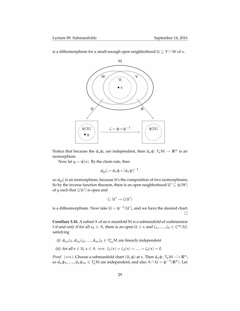
is a diffeomorphism for a small enough open neighborhood U ⊆ V ∩W of x.
M
VW
• x
U
ψ φ
ζ = φ ψ−1ψ(U) φ(U)
• y
Notice that because the dxφi are independent, then dxφ : TxM → Rn is anisomorphism.
Now let y = ψ(x). By the chain rule, then
dyζ = dxφ (dxψ)−1.
so dyζ is an isomorphism, because it’s the composition of two isomorphisms.So by the inverse function theorem, there is an open neighborhood U ′ ⊆ ψ(W)
of y such that ζ(U ′) is open and
ζ : U ′ → ζ(U ′)
is a diffeomorphism. Now take U = ψ−1(U ′), and we have the desired chart.
Corollary 3.10. A subsetA of an n-manifoldM is a submanifold of codimension` if and only if for all x0 ∈ A, there is an open U 3 x and ζ1, . . . , ζ` ∈ C∞(U)
satisfying
(i) dx0ζ1,dx0ζ2, . . . ,dx0ζ` ∈ T ∗x0M are linearly independent
(ii) for all x ∈ U, x ∈ A ⇐⇒ ζ1(x) = ζ2(x) = . . . = ζ`(x) = 0.
Proof. (=⇒). Choose a submanifold chart (U,φ) at x. Then dxφ : TxM∼
−→ Rn,so dxφ1, . . . ,dxφm ∈ T ∗xM are independent, and also A ∩U = φ−1(Rk). Let
29

Lecture 10: Submanifolds September 16, 2016
ζ1 = φk+1, ζ2 = φk+2, . . ., ζ` = φn. It can be verified that this choice offunctions works.
(⇐=). Conversely, put φk+1 = ζ1, . . . ,φn = ζ`. Then complete the covec-tors
dxφk+1 = dxζ1, . . . ,dxφn = dxζ` ∈ T ∗xM
to a basis of T ∗xM, say
α1, . . . ,αk,αk+1 = dxφk+1, . . . ,αn = dxφn ∈ T ∗xM.
So by Lemma 3.12 there are functions φ1, . . . ,φk ∈ C∞(U) such that for asufficiently small enough open U 3 x, we have
dxφ1 = α1, . . . ,dxφk = αk.
By the previous theorem, φ = (φ1, . . . ,φn) : U→ Rn is a chart (after possiblyshrinking U), and U∩A = φ−1(Rk).
Remark 3.11.
(1) Keep the same setup as in Corollary 3.10. Let ζ = (ζ1, . . . , ζ`) ∈ C∞(U, R`).Then Item (i) is equivalent to dx0ζ : Tx0M→ R` surjective, and Item (ii) isequivalent to U∩A = ζ−1(0).
(2) Tx0A consists of all v ∈ Tx0Mwith
dx0ζ1(v) = . . . = dx0ζ`(v) = 0.
So Tx0A = v ∈ Tx0M | dx0ζ(v) = 0 = ker(dx0ζ).
In the special case ofM = Rn, dx0ζmanifests itself as the Jacobian matrixDζx0 , which is an `× n matrix. Then dx0ζj = (Dζj)x0 is the j-th row ofDζx0 . So
Tx0A = ker(Dζ(x0)) = ker((Dζ1)x0)∩ . . .∩ ker((Dζ`)x0)
= 〈∇x0ζ1〉⊥ ∩ . . .∩ 〈∇x0ζ`〉⊥,
where 〈v〉 denotes the linear subspace generated by the vector v ∈ R`.
Lemma 3.12. For every α ∈ T ∗xM, there is a germ [f]x ∈ C∞M,x such that dxf = α.
That is, dx : C∞M,x → T ∗xM is surjective.
Proof. On the next homework.
30

Lecture 10: Rank September 16, 2016
3.1 Rank
Definition 3.13. LetM andN be manifolds of dimensionm and n, respectively.Let F : M→ N be smooth. The rank of F at x ∈M is
rankx(F) = rank(TxF : TxM→ TF(x)N) = dim(TxF(TxM)).
Remark 3.14 (Recall). A linear map T : Rm → Rn of rank r ≤ min(m,n) hasanm× nmatrix representation [
Ir 0
0 0
]
with respect to suitable bases of Rm and Rn. Then in coordinates relative tothese bases,
T(x1, . . . , xm) = (x1, . . . , xr, 0, . . . , 0︸ ︷︷ ︸n−r
).
Theorem 3.15. Let f : M → N be a smooth map of smooth manifolds, m =
dim(M), n = dim(N). Let a ∈ M, r = ranka(f) = rank(Taf) ≤ min(m,n).Then there exist adapted charts (U,φ) centered at a and (V ,ψ) centered at f(a)and a smooth map g : φ(U)→ Rn−r such that
(i) ψ f φ−1(x1, . . . , xn) = (x1, . . . , xr,g(x1, . . . , xm))
(ii) g(0) = 0
(iii) Dg0 = 0
Proof. Let E = TaM and F = Tf(a)N, T = Taf : E → F, and F1 = im(T). Letr = dim F1. Choose a basis v1, . . . , vr of F1 and complete it to a basis v1, . . . , vr,vr+1, . . . , vn of F. Choose vectors u1, . . . ,ur ∈ Ewith Tui = vi for 1 ≤ i ≤ r.
Since the images of the ui’s are independent, then the ui’s must be indepen-dent themselves. So E1 = spanu1, . . . ,ur ⊆ E has dimension r, and
T |E1 : E1 → F1
is an isomorphism.Now if u ∈ E1 ∩ ker(T), then T(u) = 0, so u = 0 because u ∈ E1. Hence,
E1∩ker(T) = 0. So if we choose a basisur+1, . . . ,um of ker(T), thenu1, . . . ,ur,ur+1, . . . ,um is a basis of E by the rank-nullity theorem.
We have that
T(uj) =
vj for j ≤ r0 for j > r
31

Lecture 10: Rank September 16, 2016
The matrix of T with respect to these bases is
A =
[Ir 0
0 0
]
Let u∗1, . . . ,u∗m ∈ E∗ and v∗1, . . . , v∗n ∈ F∗ be the dual bases, with u∗i(uj) = δijand v∗i(vj) = δij. Then the dual map T ∗ : F∗ → E∗ satisfies
T ∗(v∗j ) = v∗j T = u∗j .
By Theorem 3.9, there is a chart (V ,ψ) centered at f(a) such that df(a)ψj =v∗j for j = 1, . . . ,n. Let U0 = f−1(V), this is an open neighborhood of a. So forj = 1, . . . , r, define
φj := ψj f
This choice guarantees that the following commutes.
U0 V Rm R
a f(a) 0
φj
f ψ prj
∈ ∈ ∈
Then for j = 1, . . . , r,
daφj = df(a)ψj Taf = v∗j T = u∗j
and also, φj(a) = 0 by the choice of charts. Now to make a chart at a ∈ M,choose C∞ functions φr+1, . . . ,φm ∈ C∞(U) with
φj(a) = 0, daφj = u∗j
for all j ≥ r+ 1.So by Corollary 3.10, there is an open neighborhood U ⊆ U0 of x such that
the restriction of φ = (φ1, . . . ,φr,φr+1, . . . ,φm) to U is a coordinate map onU. Hence, (U,φ) is a chart.
So let gj = ψj f φ−1 for j = r+ 1, . . . ,n and set
g = (gr+1, . . . ,gn) : φ(U)→ Rn−r.
We will verify that this choice of g is the map that we want.It’s easily seen that g(0) = 0 by the choice of charts. Moreover, for x ∈ φ(U),
we have thatψj f φ−1(x) = φj φ−1(x) = xj
32

Lecture 10: Rank September 16, 2016
for 1 ≤ j ≤ r, andψj f φ−1(x) = gj(x)
for r+ 1 ≤ j ≤ n. So
ψ f φ−1(x) = (x1, . . . , xr,g(x))
as desired.Finally, daφj = u∗j for all j implies that
daφj(ui) = δij.
So daφ(ui) = ei is the standard basis vector of Rn. Hence for j ≥ r+ 1,
D(gj)0ei =(df(a)ψj T (daφ)−1
)ei
= df(a)ψj(T(ui))
=
df(a)ψj(vi) = v
∗j (vi) = δij if i ≤ r
df(a)ψj(0) = 0 if i ≥ r+ 1
If i ≤ r, we get D(gj)0ei = δij. But j ≥ r+ 1 and i ≤ r, so the Kronecker deltavanishes here and we see that D(gj)0ei = 0 for all i.
If i ≥ r+ 1, then T(ui) = 0, so D(gj)0ei = df(a)ψj(T(ui)) = 0.Hence, D(gj)0 kills all standard basis vectors, so Dg0 = 0.
Corollary 3.16. Every a0 ∈ M has a neighborhood U such that ranka(f) ≥ranka0(f) for all a ∈ U.
This is called semicontinuity of the rank function.
Proof. Choosing charts as in Theorem 3.15, we have
ψ f φ−1(x) =
x1...xrg(x)
.
D(ψ f φ−1)x =
[Ir 0
D1gx D2gx
],
where Dgx = (D1gx,D2gx), D1gx is the partials of g with respect to x1, . . . , xr,and D2gx is the partials of gwith respect to xr+1, . . . , xm.
With this in mind, we can see that
rank(f) = rank(ψ f ψ−1) = rankD(ψ f φ−1) ≥ r.
33

Lecture 11: Rank September 19, 2016
Definition 3.17. f : M→ N has constant rank at a ∈M (or is a subimmersion)if rankb(f) = ranka(f) for b in a neighborhood of a.
Theorem 3.18 (Constant Rank Theorem). Suppose f has constant rank at a. Thenthere exist adapted charts (U,φ) centered at a and (V ,ψ) centered at f(a) suchthat
ψ f φ−1(x1, . . . , xm) = (x1, . . . , xr, 0, . . . , 0︸ ︷︷ ︸n−r
).
Proof. Choose charts (U,φ) and (V ,ψ) as in Theorem 3.15. Then f is constantrank near a if and only if f has constant rank near 0 ∈ Rm, where f = ψ fφ−1.Therefore, since
Df0 =
[Ir 0
D1g0 D2g0
],
and g(0) = 0, then we must have that D2gx = 0 for x close to 0 in Rm. Hence,g(x) is independent of xr+1, . . . , xm for x ∈ W = W1 ×W2, where W1 is aneighborhood of 0 ∈ Rr andW2 is a neighborhood of 0 ∈ Rm−r. So there is asmoooth h : W1 → Rn−r with g(x1, . . . , xm) = h(x1, . . . , xr). Hence,
ψ f φ−1(x1, . . . , xm) = (x1, . . . , xr,h(x1, . . . , xr)).
Define a shear transformation
σ : W1 ×Rn−r −→ W1 ×Rn−r
(u, v) 7−→ (u, v− h(u))
This is a diffeomorphism with inverse
σ−1(y, z) = (y, z+ h(y)).
We have that
σ ψ f φ−1(x1, . . . , xm) = (x1, . . . , xr, 0, . . . , 0).
So finally, replace ψ with σ ψ. Need also to restrict φ to U∩φ−1(W) and ψ toV ∩ψ−1(W ×Rn−r) for everything to remain well-defined.
The previous theorem is a workhorse of differential topology. There are twoextreme cases that come up quite often: namely when the rank of f is either thatof the domain or of the codomain.
34

Lecture 11: Submersions and Immersions September 19, 2016
3.2 Submersions and Immersions
Definition 3.19. Let f : M→ N be smooth. Then f is called
(a) an immersion at a ∈M if Taf : TaM→ Tf(a)N is injective.
(b) a submersion at a ∈M if Taf : TaM→ Tf(a)N is surjective.
Corollary 3.20 (Immersion Theorem). If f is an immersion at a, then rankb(f) =m for b in a neighborhood of a, and there exist adapted charts (U,φ) centeredat a and (V ,ψ) centered at f(a) with
ψ f φ−1(x1, . . . , xm) = (x1, . . . , xm, 0, . . . , 0︸ ︷︷ ︸n−m
).
Proof. If f is an immersion at a, then ranka(f) = m = dim(M). So m ≤ n andfor b close to a, the rank is bounded below by m by Theorem 3.18, but alsoabove by the number of columns, so we see that
m ≤ rankb(f) ≤ m.
Hence, rankb(f) is constant near a. Now take r = m in Theorem 3.18.
Corollary 3.21 (Submersion Theorem). If f is a submersion at a, then rankb(f) =m for b in a neighborhood of a, and there exist adapted charts (U,φ) centeredat a and (V ,ψ) centered at f(a) with
ψ f φ−1(x1, . . . , xm) = (x1, . . . , xn).
Proof. If f is a submersion at a, then ranka(f) = n = dim(N). Similarly, we seethat
n ≤ rankb(f) ≤ n
for b near a. So rankb(f) is constant near a. Now take r = n in Theorem 3.18.
Definition 3.22. If f : X→ Y, then the fiber of f over y ∈ Y is
f−1(y) = x ∈ X | f(x) = y.
Theorem 3.23 (Fiber Theorem). Let f : M→ N, dim(M) = m, dim(N) = n. Letc ∈N and A = f−1(c). Further assume that f is of constant rank r at all pointsof A.
Then the fiber f−1(c) is a closed submanifold ofM of dimension dim(A) =
m− r and the tangent bundle is equal to
TA = ker(Tf) =⊔a∈A
ker(Taf).
35

Lecture 11: Submersions and Immersions September 19, 2016
Proof. Let a ∈ A. Choose charts (U,φ) and (V ,ψ) as in Theorem 3.15, and letF ⊆ Rm be the linear subspace
F = x ∈ Rm | x1 = x2 = . . . = xr = 0 ∼= Rm−r.
Then x ∈ φ(U∩A) ⇐⇒ f(x) = 0. But
f(x) = (x1, . . . , xr, 0, . . . , 0︸ ︷︷ ︸n−r
),
so f(x) = 0 ⇐⇒ x ∈ F. SoU∩A = φ−1(F). This shows thatA is a submanifoldofM at a; up to renumbering the coordinates, (U,φ) is a submanifold chart forA. We have that dim(A) = dim(F) = m− r.
Now the following diagram commutes by the definition of Taf.
TaM TcN
Rm Rn
Taf
daφ dcψ
f=Df0
Moreover, the vertical maps are isomorphisms. Hence,
TaA = (daφ)−1(F)
= (daφ)−1(ker(f))
= ker(f daφ
)= ker(Df0 daφ)
= ker(dcψ Taf)= ker(Taf),
the last equality because dcψ is an isomorphism.
Definition 3.24. The number e(f,A) = n− r is called the excess of f at A =
f−1(c).
Remark 3.25. Interpretation of excess. Near a ∈ A, φ(A) is the solution set ofn equations inm variables,
f1(x1, . . . , xm) = 0
f2(x1, . . . , xm) = 0
...
fn(x1, . . . , xm) = 0
If the equations were functionally independent, then we would have dim(A) =
m − n. Instead, only r equations are independent, so dim(A) = m − r =
m−n+ e(f,A).
36

Lecture 12: Submersions and Immersions September 21, 2016
In the case where the excess is zero, then we have the following importantdefinition.
Definition 3.26. Call c ∈ N a regular value of f if for all a ∈ A = f−1(c), f is asubmersion at a.
Theorem 3.27 (Regular value theorem). If c ∈ N is a regular value of f, thenA = f−1(c) is a closed submanifold of dimensionm−n, and TA = ker(Tf).
Example 3.28. Let M =M(n× n, R) ∼= Rn2
be the n× n matrices with entriesin R. Then define f : M→M by f(X) = XXT . Then
f−1(I) = X ∈M | XXT = I
is the orthogonal group of n×n orthogonal matrices, denotedO(n) orO(n, R).
Claim 3.29. O(n) is a submanifold ofM of dimension n(n− 1)/2 and TIO(n) =o(n), the Lie algebra of skew-symmetric matrices.
Proof. Let N = Y ∈M | Y = YT be the subspace of symmetric matrices. Viewf as a map f : M → N. We can check that I is a regular value of f. Let A ∈ M.Then DfA : M→ N is linear. For H ∈M, what is DfAH?
f(A+H) = (A+H)(A+H)T
= AAT +AHT +HAT +HHT
= f(A) + LA(H) + R(H)
where L(H) = AHT +HAT is linear and R(H) = HHT . So, considering thematrix norms,
‖R(H)‖‖H‖ =
‖HHT ‖‖H‖ ≤ ‖H‖
2
‖H‖ = ‖H‖ −−−−→H→0 0
So we have thatDfA(H) = LA(H) = AH
T +HAT .
To check that f is a submersion at A ∈ O(n), we need to know that LA issurjective. So let B ∈ N. We want to solve
AHT +HAT = B
for H. To do this, rewrite the above as
AHT +HAT = 12B+ 1
2B.
Then half of the above equation is easy to solve. If we set HAT = 12B, then
H = HATA = 12BA.
37

Lecture 12: Embeddings September 21, 2016
This H = 12BA satisfies
AHT +HAT = 12AA
TB+ 12BAA
T = B
because B is symmetric.Hence, I is a regular value of f, because f−1(I) = O(n) and f is a submersion
at each point in O(n).Therefore,
dim(O(n)) = dim(M) − dim(N) = n2 − 12n(n+ 1) = 1
2n(n− 1).
Then TIO(n) = ker(Df(I)) = ker(H 7→ HT +H), which is all of the skew-symmetric matrices.
Remark 3.30. O(n) is our first example of a Lie group. For any A ∈ O(n),
1 = det(AAT ) = det(A)2 =⇒ det(A) = ±1.
So O(n) has two connected components, namely the preimage under det of +1and the preimage under det of −1.
The special orthogonal group is
SO(n) = A ∈ O(n) | det(A) = 1,
the connected component of O(n) of determinant 1matrices is one coset, andthe other connected component of O(n) is the coset
A0 SO(n) = A ∈ O(n) | det(A) = −1,
where A0 is the matrix
A0 =
−1
1
. . .1
Remark 3.31. Another method we could use to prove Claim 3.29 would be tocheck that f is a subimmersion of appropriate rank. We’ll do this later when wetalk about Lie groups.
3.3 Embeddings
Definition 3.32. f : M → N is an embedding if it is an immersion (that is, animmersion at every point ofM) and a homeomorphism onto its image.
Remark 3.33. Equivalently, f : M→ N is an embedding if
38

Lecture 12: Embeddings September 21, 2016
(i) f is injective,
(ii) Taf is injective for all a ∈M, and
(iii) f−1 : f(M)→M is continuous.
Theorem 3.34 (Embedding Theorem).
(i) The inclusion of a submanifold i : A→M is an embedding.
(ii) If f : P → M is an embedding, then A− f(P) is a submanifold of M andf : P → A is a diffeomorphism and TA = Tf(TP).
Proof.
(i) Recall that Ti is injective, so i is an immersion. By definition, the inclusionis injective. Also the topology on A is the subspace topology inducedby its smooth structure is the subspace topology inherited from M. Inparticular, this means that i is a homeomorphism onto its image.
(ii) Let k = dim(P) and n = dim(M). Then let p ∈ P, a = f(p) ∈ A. Theimmersion theorem gives adapted charts (U,φ) centered at p and (V ,ψ)centered at a such that
ψ f φ−1(x1, . . . , xk) = (x1, . . . , xk, 0, . . . , 0)
is the inclusion Rk → Rn.
Rk( )
φ(U)
P
( )•p
φ
ψ f φ−1
f
MA V
•a
ψ
ψ(V)
Rn
We would like that f(U) = A∩V and f(U) = ψ−1(Rk). This may howeverfail, so first replace (V ,ψ) by (V0,ψ0) where V0 = V ∩ψ−1(φ(U)×Rk)
and ψ0 = ψ|V0 .
39

Lecture 13: Embeddings September 23, 2016
To get f(U) = A∩ V0 use the fact that f is a homeomorphism onto A. Sotehre is open V ′ ⊆M withf(U) = A∩ V ′. Replace (V0,ψ0) with (V1,ψ1)where V1 = V0 ∩ V ′ and ψ1 = ψ0|V1 . Now we have that f(U) = A ∩ V1and f(U) = ψ−1
1 (Rk).
Then (V1,ψ1) is a submanifold chart for A at a. The map f−1 : A→ P isrepresented near a by
φ f−1 ψ−1 : ψ(A∩ V1) −→ φ(U)
x 7−→ x
noting that both ψ(A ∩ V1) and φ(U) are contained in Rk. So f−1 issmooth, so f is a diffeomorphism and Tf : TP → TM sends TP onto TA.
Example 3.35 (Non-example). Let P = (−π2 , 3π2 ),M = R2, and
f(t) =
(cos(t)
cos(t) sin(t)
).
We have chosen the domain such that this is injective. The graph of this functionfor t ∈ P is the lemniscate.
f is an injective immersion, and
f ′(t) =
(− sin(t)
− sin2(t) + cos2(t)
)6=(0
0
).
Then f−1 : f(P) → P is not continuous: f is not an embedding, f(P) is not asubmanifold.
40

Lecture 13: Embeddings September 23, 2016
Example 3.36 (Non-example). Let P = R andM = S1 × S1 the 2-torus. Let
f(t) =
(eit
eiαt
).
Hence we think of S1 as the unit circle z ∈ C | |z| = 1. Then
f ′(t) =
(ieit
iαeiαt
)6=(0
0
),
so f is an immersion.If α = p
q ∈ Q, then f is not injective: f(t) = f(t+ 2πq). But f descends to amap
f :R/2πqZ
→ S1 × S1
called a torus knot. f is an injective immersion, and in fact f is an embeddingbecause the inverse is continuous. To check that f−1 : f(R) → R/2πqZ is con-tinuous, one must check that if C ⊆ R/2πqZ is closed, then f(C) is closed inS1 × S1. True because R/2πqZ
∼= S1 is compact.
Fact 3.37 (Kronecker). If α 6∈ Q, then f is injective and A = f(P) is dense in M,so it is certainly not a submanifold.
The plot of the torus knot f(t) = (eit, eiαt) for α irrational and 0 ≤ t ≤ 200(left) or 0 ≤ t ≤ 500 (right). Notice that the as the upper bound on t grows
larger, more of the torus is filled in.
Definition 3.38. An immersed submanifold of a manifold M is a pair (P, f)where P is a manifold and f : P →M is an injective immersion.
Then f : P → A = f(P) is a continuous bijection, but f−1 : A → P is notnecessarily continuous for the subspace topology on A.
Remark 3.39. Identifying PwithA, we see an immersed submanifold is a subsetA ofM equipped with a smooth structure such that the inclusion i : A→M isan immersion.
But the topology onA induced by this smooth structure may be finer (bigger,stronger) than the subspace topology.
41

Lecture 14: Vector Fields September 26, 2016
4 Vector Fields
LetM be an n-manifold, and let π = πM : TM→M the tangent bundle projec-tion. Then for any a ∈M, π−1(a) = TaM for all a ∈M.
Definition 4.1. A vector field on M is a smooth section of π, that is, a mapξ : M → TM satisfying π ξ = idM. So ξ(a) ∈ TaM for all a ∈ M. We oftenwrite ξ(a) = ξa.
Definition 4.2. A point a ∈M is a zero or equilibrium of ξ if ξa = 0 ∈ TaM.
Let c = (U,φ) be a chart onM. Then ξ(U) ⊆ TU = π−1(U), so c and Tc areadapted for ξ. An expression for ξ in coordinates is then
Tφ ξ φ−1 : φ(U) −→ Tφ(U) = φ(U)×Rn
So this defines a vector field on φ(U) ⊆ Rn. For each x ∈ φ(U),
Tφ ξ φ−1(x) = (x,h)
for some h ∈ R. We write h = ξ(x), with ξ : φ(U)→ Rn.
Definition 4.3. A vector field ξ is smooth if and only if ξ is smooth for all chartsc onM.
Remark 4.4. This meshes with our definition of smooth morphisms of mani-folds: f : M → N is smooth if and only if it’s expression in any pair of chartsis smooth as a map Rm → Rn. We see that ξ is smooth if and only if it’sexpression Tπ ξ φ−1 is smooth, if and only if ξ is smooth.
Definition 4.5. For vector fields ξ,η and a function f : M→ R, we define vectorfields ξ + η and fξ by (ξ + η)(a) = ξ(a) + η(a) and (fξ)(a) = f(a)ξ(a).
With respect to a chart cwe have (ξ + η) = ξ + η and (fξ) = f ξ.
Definition 4.6 (Notation). T (M) =ξ : M→ TM | π ξ = idM, ξ is smooth
Remark 4.7. T (M) is a module over the algebra C∞(M).
Definition 4.8. A k-frame on M is an ordered k-tuple (ξ1, . . . , ξk) of smoothvector fields onM such that for all a ∈M, (ξ1)a, . . . , (ξk)a ∈ TaM are linearlyindependent.
Example 4.9. A 1-frame on M is a nowhere vanishing vector field ξ. That is,ξa 6= 0 for all a.
Definition 4.10. An n-manifoldM is called parallelizable if it has an n-frame.
42

Lecture 14: Independent vector fields on spheres September 26, 2016
Let kM = maxk |M has a k-frame
≤ dim(M).M is parallelizable if and
only if kM = dim(M).
Example 4.11. Let M = U be an open subset of Rn. A smooth vector field onU is a smooth map ξ : U → TU = U×Rn of the form ξ(x) = (x, ξx), whereξ : U→ Rn is smooth.U is parallelizable: the constant vector fields e1, . . . , en : U → Rn serve as
an n-frame for U.
Example 4.12. A Lie groups G is parallelizable by a basis of the associated Liealgebra g = T0G, left-or-right-translated around G.
4.1 Independent vector fields on spheres
Theorem 4.13 (F. Adams, 1962). Let M = Sn−1. Let m = max` | 2` divides n.Write m = 4b+ a, with b ∈ Z, a ∈ 0, 1, 2, 3. Let ρ(n) = 2a + 8b. This is theRadon-Hurwitz number. Then
kSn−1 = ρ(n) − 1.
Here are the first 10 values of ρ(n). This counts the number of independentvector fields on a sphere. If n is odd, then m = 0, a = b = 0, so kM = 0, andevery smooth vector field on an even dimensional sphere has zeros.
n 1 2 3 4 5 6 7 8 9 10 · · ·ρ(n) 1 2 1 4 1 2 1 8 1 2 · · ·
Sn−1 is parallelizable if and only if kSn−1 = n− 1 if and only if ρ(n) = n.
Theorem 4.14 (Kervaire, 1956). ρ(n) = n if and only if n = 1, 2, 4, 8. Therefore,Sn−1 is parallelizable if and only if n = 1, 2, 4, 8.
The reason that this only works for n = 1, 2, 4, 8 is that there are only fourreal division algebras: R, C, the quaternions, and the octonions. This will be onyour homework.
Remark 4.15. Some of these spheres have Lie group structures. S1 is the Liegroup U(1), and S3 can be identified with the unit quaternions, which is alsoSU(2). S7 is the unit octonions, but they are not associative, so there is no Liegroup structure on S7.
43

Lecture 14: Flows September 26, 2016
4.2 Flows
Recall that for γ : J→M, where J ⊆ R is an open interval, the tangent map is
Ttγ : TtR = t×R→ Tγ(t)M.
We put γ ′(t) = Ttγ(t, 1).
Definition 4.16. Let ξ ∈ T(M). An integral curve or trajectory of ξ is a smoothmap γ : J→M, which satisfies γ ′(t) = ξγ(t) for all t ∈ J.
We say that γ starts at a ∈M if 0 ∈ J and γ(0) = a.
For s ∈ R let J+ s = t+ s | t ∈ J.
Lemma 4.17 (Time Translation Lemma). Let γ : J → M be a trajectory for ξ.Define δ : J− s → M by δ(t) = γ(t+ s). Then δ is a trajectory. If s ∈ J, then δstarts at a = γ(s).
Proof. By the chain rule, δ ′(t) = γ ′(t + s) = ξγ(t+s) = ξδ(t). If s ∈ J, then0 ∈ J− s and δ(0) = γ(s) = a.
What if there’s a hole in our manifold, and a mouse running along a trajectorywould fall into that hole? Then we cannot extend the map γ : J→M to all of R.The question is when we can extend a trajectory to all of R.
Definition 4.18. Define a partial ordering on trajectories as follows. If γ1 : J1 →M and γ2 : J2 →M are trajectories, then γ1 ≤ γ2 if J1 ⊆ J2 and γ2|J1 = γ1.
A trajectory γ : J → M of ξ is maximal if it is maximal with respect to thispartial ordering. That is, if for any other trajectory γ1 : J1 →M with J1 ⊇ J andγ1|J = γ, we have J = J1.
Essentially, maximality of a trajectory means that it cannot be extended anyfurther. The initial value problem for ξ is to find for each a ∈ M a trajectoryγ : J→M such that γ ′(t) = ξγ(t) starting at a, γ(0) = a, which is maximal. Thenext theorem says that the initial value problem has a solution for any a ∈M.
Theorem 4.19 (Existence and Uniqueness). For each a ∈ M, there is a uniquemaximal trajectory starting at a.
Proof. To settle existence, choose a chart (U,φ) at a. Then write the vector fieldin coordinates: for any path γ : J→M, we get a path
γ = φ γ : J −→ φ(U) ⊆ Rn.
Also, write
Tφ ξ φ−1 : φ(U) −→ φ(U)×Rn
x 7−→ (x, ξx)
44

Lecture 15: Flows September 28, 2016
where ξ : φ(U) → Rn is the expression for ξ in the chart (U,φ). Then γ is atrajectory of ξ starting at a if and only if
γ ′(t) = ξγ(t)
γ(0) = φ(a),(5)
which is a vector-valued ordinary differential equation, and ξγ(t) is smooth.By the existence theorem for solutions to ODE’s, a solution γ : J → φ(U)
exists. Compose with φ−1 to the desired γ = φ−1 γ : J→ U starting at a.
To settle uniqueness, let γ1 : J1 → M and γ2 : J2 → M be two trajectoriesstarting at a solving the ODE (5).
Let I = t ∈ J1 ∩ J2 | γ1(t) = γ2(t). Then 0 ∈ I because γ1(0) = a = γ2(0).Let Γ(t) = (γ1(t),γ2(t)). Notice that Γ : J1 ∩ J2 →M×M is smooth.
We have that I = Γ−1(∆M) where ∆M = (x, x) | x ∈ M. Since M isHausdorff, ∆ is closed. Hence, I is closed in J1 ∩ J2 as the inverse image of aclosed set under a smooth map.
The uniqueness theorem for solutions to ODE’s, applied to (5), so I is open.Hence, I = J1 ∩ J2 as a connected, nonempty component of J1 ∩ J2. Therefore,γ1 = γ2 on J1 ∩ J2.
Finally, to show maximality, let γα : Jα → M | α ∈ A be the collectionof trajectories starting at a. For all α,β ∈ A, we have γα = γβ on Jα ∩ Jβ bythe argument for uniqueness. So define J =
⋃α∈A Jα. This is an open interval
containing a, and γ(t) = γα(t) for all t ∈ J and α ∈ A such that t ∈ Jα. Then γis well-defined, smooth, and maximal by construction.
Corollary 4.20. Let γ : J→M be the maximal trajectory of ξ starting at a ∈M.Let s ∈ J, and b = γ(s) and δ(t) = γ(t+ s). Then δ : J− s → M is the uniquemaximal trajectory starting at b.
Proof. Combine the Time Translation Lemma (Lemma 4.17) and the previoustheorem (Theorem 4.19).
Definition 4.21. For a ∈ M, let 0 ∈ Da = Da(ξ) ⊆ R be the domain of themaximal trajectory starting at a. The flow domain of ξ is
D = D(ξ) = (t,a) | t ∈ Da ⊆ R×M.
The flow of ξ is the map θ : D → M defined by θ(t,a) = γ(t), where γ is themaximal trajectory of ξ starting at a.
45

Lecture 15: Flows September 28, 2016
M
Rn
•D
a
Remark 4.22 (Notation). Also put Dt = a ∈ M | (t,a) ∈ D, and θt(a) =
θa(t) = θ(t,a) for t ∈ R, a ∈M. Define
θa : Da →M
θt : Dt →M
by θ(t,a) = θt(a) = θa(t). Finally, note that
t ∈ Da ⇐⇒ (t,a) ∈ D ⇐⇒ a ∈ Dt.
Example 4.23. If M = R, and ξ(x) = x2, then what is the flow of ξ? We solvethe initial value problem for ξ:
x ′(t) = x(t)2
x(0) = x0
This is an ODE that we can solve. We have
x ′(t)
x(t)2= 1
so integrating, we see that
−1
x(t)= t+C
for some constant C. Hence,
x(t) = −1
t+C.
Substituting the inital value x(0) = x0, we see that C = − 1x0
. Therefore,
x(t) =1
−t+ 1x0
=x0
1− tx0
46

Lecture 15: Flows September 28, 2016
is the solution. The flow isθ(t, x) =
x
1− tx.
The domain of this flow is for x0 = 0, x(t) = 0 for all t, so D0 = R. This is theequilibrium solution. For x0 > 0, x(t) exists for t < 1
x0, so
Dx0 = (−∞, 1x0 ).
For x0 < 0, we have thatDx0 =
(1x0
,∞) .
M
R
Ds
s
x0Dx0
Dx1x1
Theorem 4.24.
(i) The flow domain D ⊆ R ×M of ξ is open and the flow θ : D → M
is smooth. In particular for each t ∈ R the set Dt ⊆ M is open andθt : Dt →M is smooth.
(ii) Dθ(t,a) = Da − t for all (t,a) ∈ D.
(iii) We have that Ds+t ⊇ Ds ∩ θ−1s (Dt) and on Ds ∩ θ−1s (Dt) the flow law
θs+t = θt θs (6)
holds.
(iv) D0 =M and θ0 = idM.
Proof.
(i) We will only sketch the proof of this, because it’s analysis that we don’tneed to think about. Use charts to reduce to the case of M = U ⊆ Rn
open. Then the result is true by the theory of ODE’s: for each a ∈ U, there
47

Lecture 16: Flows September 30, 2016
is an open neighborhood V of a in U and ε > 0 such that for all x ∈ V ,the trajectory θ(t, x) exists for all t ∈ (−ε, ε). This shows D is open. Also,θ(t, x) depends smoothly on t and x.
(ii) Let γ(t) = θ(t,a). For some s ∈ Da, let δ(t) = γ(t+ s). The domainof δ is Da − s by time translation; δ starts at γ(s) = θ(s,a). That is,δ(t) = θ(t, θ(s,a)). The definition interval of D is Dθ(s,a).
(iii) Fix a ∈M; let γ, δ be as in (ii). We get
γ(t+ s) = θ(t, θ(s,a)).
That is,θ(t+ s,a) = θ(t, θ(s,a)).
We can rewrite this as
θs+t(a) = θt(θs(a)).
For this to hold we must have s ∈ Da and t ∈ Da − s = Dθ(s,a). This istrue if and only if a ∈ Ds and θ(s,a) ∈ Dt. Again, this is true if and onlyif a ∈ Ds and a ∈ θ−1s (Dt).If t, s satisfy these conditions, then s+ t ∈ Da. That is, a ∈ Ds+t.
(iv) Clear from the results of the other parts.
Corollary 4.25. θt(Dt) = D−t and θt : Dt → D−t is a diffeomorphism withinverse θ−t.
Proof. By Theorem 4.24(iii), for all (s, t,a) ∈ R×R×M,
s+ t ∈ Da ⇐⇒ s ∈ Da − t(iii)= Dθ(t,a) ⇐⇒ θ(t,a) ∈ Ds ⇐⇒ θt(a) ∈ Ds.
Set s = −t. Then0 ∈ Da ⇐⇒ θt(a) ∈ D−t.
But we always have that 0 ∈ Da, so θt(Dt) ⊆ D−t.Then the flow law (6) tells us that
θ−t(θt(a)) = θ0(a) = a
and replacing t by −t, we get that θt θ−t = idD−t.
Definition 4.26. ξ is complete if D = D(ξ) = R×M, that is, Da = R for all a,or Dt =M for all t.
48

Lecture 16: Flows September 30, 2016
Remark 4.27. In the case that the flow of ξ is complete, then each θt is a dif-feomorphism M → M. That is, θt ∈ Diff(M), the group of diffeomorphismsM→M, and in this case t 7→ θt is a homomorphism R→ Diff(M) by the flowlaw (6). It also defines an action of R onM.
When is a vector field complete? Are there easy criteria for this?
Lemma 4.28 (Uniform Time Lemma). If there is ε > 0 such that (−ε, ε)×M ⊆ D,then ξ is complete.
M
Rn
•D
ε
Proof. Let a ∈M. Let s = sup(Da). Suppose s <∞.
( )|s− ε st0
Da
Then let t0 ∈ (s−ε, s) ∈ Da. Let b = θ(ta,a). Since (−ε, ε) ⊆ Db = Dθ(t0,a) =
Da − t0, we have (t0 − ε, t0 + ε) ⊆ Da. But t0 + ε > s, which is a contradiction.So s =∞. Similarly, inf(Da) = −∞.
Definition 4.29. The support of ξ is
supp(ξ) =a ∈M | ξa 6= 0a
Theorem 4.30. If supp(ξ) is compact, then ξ is complete.
Proof. Let K = supp(ξ). If a 6∈ K, then ξa = 0, so θ(t,a) = a for all t andDa = R. For every a ∈ K there is εa > 0 and a neighborhood Ua of a such that(−ε, ε)×Ua ⊆ D. That is to say that for all b ∈ Ua, we have (−εa, εa) ⊆ Db.
Cover K by finitely many Ua1 , . . . ,Uap ; put ε = minεa1 , . . . , εap . Then(−ε, ε) ⊆ Da for all a ∈M.
Now apply the uniform time Lemma 4.28.
49

Lecture 17: Derivations, Revisited October 03, 2016
Corollary 4.31. On a compact manifold every vector field is complete.
Example 4.32. An example of a complete vector field: linear vector fields onvector spaces.
Let ξ : Rn → Rn be a linear map with matrix A. The flow of ξ is given byθ : R×Rn → Rn, that is, the solution to the differential equation
x ′(t) = ξ(x(t)) = Ax(t)
x(0) = x0
The solution to this equation is
x(t) = exp(tA)x0,
where exp is the matrix exponential. This is defined for all t.A time-dependent linear vector field on Rn is a vector field ξ on R×Rn
of the form
ξ(t, x) =(d
dt,A(t)x
)where A : R→M(n, R) is a smooth map. Such a vector field is also complete.
4.3 Derivations, Revisited
Let A be a commutative unital ring and let B be a commutative A-algebra withidentity. Let C be a B-module. Think of A as the scalars, (e.g. A = R) and B asthe functions (e.g. B = C∞(M, R)), and C as the vector valued functions (e.g.C∞(M, Rk) or T (M)).
Definition 4.33. An A-derivation of B into C is a map ` : B→ C satisfying
(a) A-linearity: `(a1b1 + a2b2) = a1`(b1) + a2`(b2), and
(b) the Leibniz rule: `(b1b2) = `(b1)b2 + b1`(b2).
for all ai ∈ A and bi ∈ B.
Remark 4.34. We should really write b2`(b1) instead of `(b1)b2 because C is a(left) B-module, but if we were working in the non-commutative case then thiswould be wrong. But in our case, B is commutative so we may pretend that C isa B-bimodule with the left and right actions coinciding. In the noncommutativecase, we must add the assumption that C is a B-bimodule.
Definition 4.35. The set DerA(B,C) is the set of all A-derivations of B into C.It is a B-module as well as an A-module; if b1,b2 ∈ B and `1, `2 ∈ DerA(B,C),then b1`1 + b2`2 is also a derivation for B commutative.
50

Lecture 17: Derivations, Revisited October 03, 2016
Lemma 4.36. If ` ∈ DerA(B,C), then `(a1B) = 0 for all a ∈ A.
Proof. `(1B) = `(1B1B) = `(1B)1B + 1B`(1B) = 2`(1B) =⇒ `(1B) = 0.
Example 4.37. Let a ∈M and let B = C∞M,a be the algebra of germs at a, and
C = R. Here A = R. Recall that we have an evaluation map
C∞M,a C = R
[f] f(a)
eva
This is an algebra homomorphism. This makes C into a B-module, via
[f] · c = f(a)c.
We called DerR(C∞M,a, R) the derivations ofM at a. The map
TaM DerR(C∞M,a, R)
v La(v)
La
is an isomorphism given by
La(v)([f]) = daf(v).
Definition 4.38. Let B = C∞(M) = C. We call DerR(C∞(M)) the derivations
ofM.
Definition 4.39. Each ξ ∈ T (M) defines a derivation Lξ ofM, given by
Lξ(f) = df(ξ).
This is the Lie derivative or directional derivative of f along ξ.
That is, Lξ(f) is the function defined by
Lξ(f)(a) = daf(ξa),
and Lξ satisfies the Leibniz rule.
Remark 4.40. We need to check that Lξ(f) is smooth. We check this in a chart(U,φ), where we may write
f = f φ−1.
Recall that(Tφ ξ φ−1)(x) = (x, ξ(x)),
51

Lecture 17: Derivations, Revisited October 03, 2016
so thatTφ ξ φ−1 = idφ(U) × ξ,
where ξ : φ(U)→ Rn is smooth. Then
Lξ(f)(a) = daf(ξa) = D(f)φ(a)(ξφ(a))
for all a ∈ U. Since f, ξ are smooth, then so is Lξ(f).
Theorem 4.41. The map L : T (M) → DerR(C∞(M)) defined by ξ 7→ Lξ is an
isomorphism.
To prove this theorem, we will first need a few analysis lemmas.
Lemma 4.42 (Existence of Smooth Step Functions). For all 0 < p < q there is asmooth function λ : Rn → [0, 1] with
λ(x) =
1 for ‖x‖ < p0 for ‖x‖ > q.
The function λ looks like this:
Proof of Lemma 4.42. Define
α(x) =
e−1/x for x > 0
0 for x ≤ 0.
We can show that α is in fact smooth! Then α(k)(0) = 0 for all k ≥ 0; we say thatα is flat at 0. The k-th Taylor polynomial of α at x = 0 is the zero polynomial.
52

Lecture 17: Derivations, Revisited October 03, 2016
Define β : R→ [0,∞) by β(x) = α(x− p)α(q− x).
Define γ : R→ [0, 1] by
γ(x) =
∫qx β(t)dt∫qp β(t)dt
.
Then γ is C∞.Finally, let λ(x) = γ(‖x‖). This works.
Recall from Definition 4.29 that the support of f ∈ C∞(M) is
supp(f) = x ∈M | f(x) 6= 0
Lemma 4.43 (Extension Lemma). For every a ∈M, the restriction map
C∞(M) C∞M,a
f [f]a
is surjective.
Proof. Let [g]a ∈ C∞M,a. Then there is g ∈ C∞(U), where U is an open neighbor-
hood of a. We will cook up a global function f onM that has the same germ asg at a.
Without loss, we may assume that U is the domain of a chart (U,φ) centeredat a. Choose 0 < p < q such that Bp(0) ⊆ Bq(0) ⊆ φ(U). Choose λ as in theprevious laemma, and let ρ = λ φ ∈ C∞(U). Then
supp(ρ) = φ−1(Bq(0))
is compact and hence closed inM (becauseM is Hausdorff).Hence V = M \ supp(ρ) is open and U,V form an open cover of M. Now
define
f =
0 on V
ρg on U
On U ∩ V , ρg = 0, so f is well-defined, and f is smooth on U and on V , so fis smooth. Finally, f = g on a sufficiently small neighborhood of a, namelyφ−1(Bq(0)), so [f]a = [g]a.
53

Lecture 18: Intermezzo: Point-set topology of Manifolds October 05, 2016
Remark 4.44. Taking g = 1 in the Extension Lemma (Lemma 4.43), we get theexistence of smooth bump functions onM, corresponding to ρ in the previousproof. This leads to the next lemma.
Lemma 4.45 (Bump Function Lemma). For each a ∈M and every neighborhoodU of a, there is a smooth ρ ∈ C∞(M) with supp(ρ) ⊆ U and ρ = 1 in aneighborhood of a.
Lemma 4.46 (Locality of Derivations). Let ` ∈ DerR(C∞(M)) and f ∈ C∞(M).
Let U ⊆M be open. If f = 0 on U, then `(f) = 0 on U.
Proof. Let a ∈ U, ρ ∈ C∞(M) a bump function at a, supported on U. Thenρf = 0, so
f = (ρ+ (1− ρ))f = (1− ρ)f.
So
`(f) = `((1− ρ)f) = `(1− ρ)f+ (1− ρ)`(f).
This vanishes on a neighborhood of a. But the argument holds for all a ∈ U, so`(f) = 0 on U.
Proof Sketch of Theorem 4.41. The map ξ 7→ Lξ is evidently R-linear.To check injectivity, suppose Lξ = 0. Then for all f ∈ C∞(M),
Lξ(f) = df(ξ) = 0.
Let a ∈ M, and evaluate this at a. By Lemma 4.43, eva : C∞(M) → C∞M,a is
surjective, so for all [f]a ∈ C∞M,a,
La(ξa)([f]a) = daf(ξa) = 0.
Now using the pointwise version of the isomorphism La : TaM ∼= Dera(M) =
DerR(C∞M,a, R), we see that ξa = 0 ∈ TaM. So ξ = 0.
To check surjectivity, use locality of derivations and using charts, reduceto the case where M = U is open in Rn. Then the isomorphism L : T (M) →Der(M) is another case of Taylor’s theorem. (This is on the homework).
5 Intermezzo: Point-set topology of Manifolds
This section is some annoying business that we’ve been postponing.
54
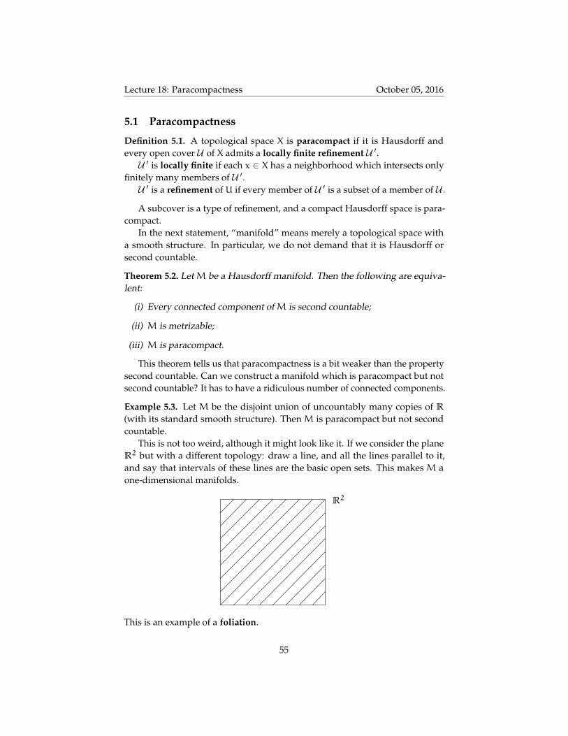
Lecture 18: Paracompactness October 05, 2016
5.1 Paracompactness
Definition 5.1. A topological space X is paracompact if it is Hausdorff andevery open cover U of X admits a locally finite refinement U ′.U ′ is locally finite if each x ∈ X has a neighborhood which intersects only
finitely many members of U ′.U ′ is a refinement of U if every member of U ′ is a subset of a member of U .
A subcover is a type of refinement, and a compact Hausdorff space is para-compact.
In the next statement, “manifold” means merely a topological space witha smooth structure. In particular, we do not demand that it is Hausdorff orsecond countable.
Theorem 5.2. Let M be a Hausdorff manifold. Then the following are equiva-lent:
(i) Every connected component ofM is second countable;
(ii) M is metrizable;
(iii) M is paracompact.
This theorem tells us that paracompactness is a bit weaker than the propertysecond countable. Can we construct a manifold which is paracompact but notsecond countable? It has to have a ridiculous number of connected components.
Example 5.3. Let M be the disjoint union of uncountably many copies of R
(with its standard smooth structure). Then M is paracompact but not secondcountable.
This is not too weird, although it might look like it. If we consider the planeR2 but with a different topology: draw a line, and all the lines parallel to it,and say that intervals of these lines are the basic open sets. This makes M aone-dimensional manifolds.
R2
This is an example of a foliation.
55

Lecture 18: Paracompactness October 05, 2016
Proof Sketch of Theorem 5.2. (i) =⇒ (ii). Let C be a connected component ofM.Then C is Hausdorff and second countable. M is also locally compact, soM isregular. For each x ∈M and each closed subset A ⊆M with x 6∈ A, there areopen sets U,V with x ∈ A, A ⊆ V , and U∩ V = ∅.
So now by Urysohn’s Metrization Theorem C is metrizable. So every com-ponent C of M is metrizable, so M is metrizable. Why? For each connectedcomponent C, let dC be a metric on C. Let
δC(x,y) =dC(x,y)
1+ dC(x,y),
then δC is a metric on C that defines the same topology. Define
d(x,y) =
δC(x,y) if x,y are in the same connected component C
1 otherwise.
Then d is a metic compatible with the topology onM.(ii) =⇒ (iii). Every metrizable space is paracompact (look it up!)(iii) =⇒ (i). We may assume without loss thatM is connected. Every point
in M has a second countable neighborhood by the paracompact assumption. Toget global second countability, we show thatM is σ-compact, that is, a countableunion of compact sets.M has an open cover U whose members U have compact closure. By para-
compactness, we may replace U by a refinement that is locally finite. So assumeU is locally finite. Let ∅ 6= U0 ∈ U . Then U0, being compact, intersects onlyfinitely many members of U , sayU1,U2, . . . ,Un1 . Likewise,U0 ∪U1 ∪ . . .∪Unintersects only finitely many members of U , say Un1+1, . . . ,Un2 .
Continuing in this way, we get a sequence U0,U1,U2, . . . in U , with∞⋃j=0
Uj =∞⋃j=0
Uj.
The collection Ujj∈N is locally finite, and therefore Ujj∈N is locally finite.The union of a locally finite family of closed sets is closed, so this implies that
∞⋃j=0
Uj
is closed. On the other hand, ∞⋃j=0
Uj =∞⋃j=0
Uj
is open, so
M =∞⋃j=0
Uj.
56

Lecture 19: Partitions of Unity October 07, 2016
Hence,M is σ-compact. Global second-countability follows.
Example 5.4. Letω1 be the first uncountable ordinal. The elements ofω1 areall countable ordinals. The long ray is
R = ω1 × [0, 1)
equipped with lexicographic order(a, s) < (b, t) if a < b
(a, s) < (a, t) if s < t
and the order topology (subbasis consisting of all segments R<x and R>x).R is a connected 1-manifold with boundary point (0, 0). The long line is
obtained by gluing two copies of R together along their boundary.The long line is not second countable, so it is not paracompact.
For the purposes of differential geometry, however, this example is generallyuseless.
5.2 Partitions of Unity
Definition 5.5. Let U = Ui | i ∈ I be an open cover ofM. A partition of unitysubordinate to U is a family of smooth functions λi : M → [0, 1] | i ∈ I suchthat
(a) supp(λi) ⊆ Ui,
(b) supp(λi) | i ∈ I is locally finite,
(c)∑i∈I
λi = 1.
Remark 5.6. Note that (b) implies that for any a ∈M, there is a neighborhoodV of a such that only finitely many λi are nonzero on V , so the sum
∑i∈I λi(a)
make sense. Moreover, for any J ⊆ I the sum∑i∈J λi is well-defined and
smooth.
Theorem 5.7. Let M be paracompact and let U be an open cover. Then thereexists a partition of unity subordinate to U .
In particular, this theorem holds whenM is Hausdorff and second countable.
Lemma 5.8. LetM be paracompact. Then
(i) M is regular, and
57

Lecture 19: Partitions of Unity October 07, 2016
(ii) every open cover U = Ui | i ∈ I of M has a shrinking: a locally finiterefinement V = Vi | i ∈ I, indexed by the same set, with Vi ⊆ Ui.
Proof.
(i) Let A ⊆ M be closed, x ∈ X \A. We want to separate A and x by opensets. For each y ∈ A, choose open sets Uy, Vy with x ∈ Uy, y ∈ Vy,Uy ∩ Vy = ∅.
Then Uy,Vy | y ∈ A∪ M \ (A∪ x) is an open cover ofM. Let Wii∈Ibe a locally finite refinement. Let
J = i ∈ I |Wi ∩ Vy 6= ∅ for some y ∈ A.
Choose open U 3 x that meets only finitely many Wj for j ∈ J, sayWj1 , . . . ,Wjn . Let
U ′ = U \ (Wj1 ∪ . . .∪Wjn), W =⋃j∈JWj.
Then U ′ ∩W = ∅, U ′ 3 x is open, andW is an open neighborhood of A.
(ii) Let Ai = M \Ui. Let x ∈ Ui. Use regularity to find a neighborhoodWi,x 3 x such that Wi,x ∩A = ∅. So Wi,x ⊆ Ui. ThenW = Wi,x | i ∈I, x ∈M is an open cover of M and a refinement of U . Choose a locallyfinite refinementW ′ ofW .
ThenW ′ = W ′j | j ∈ J for some index set J. Choose f : J → I such that
W ′j ⊆Wf(j),x. for some x ∈ Uf(j). ThenW ′j ⊆ Uf(j) sinceWi,x ⊆ Ui.For i ∈ I, set
Vi =⋃
j∈f−1(i)W ′j .
BecauseW ′ is locally finite,
Vi =⋃
j∈f−1(i)W′j ⊆ Ui.
So V = Vi | i ∈ I is a shrinking of U .
Proof of Theorem 5.7. Choose a locally finite atlas (Vj,φj) | j ∈ J of M, suchthat V = Vj | j ∈ J refines U and Vj is compact with φj(Vj) is bounded in Rn.It suffices to define a partition of unity subordinate to V .
Choose a shrinkingW = Wj | j ∈ J of V . Then Wj ⊆ Vj, soWj is compact.Cover φ(Wj) with finitely many closed balls
Bj,1,Bj,2, . . . ,Bj,m(j) ⊆ φ(Wj).
58

Lecture 20: Some applications October 12, 2016
Choose smooth functions νj,k : Rn → [0, 1] such that
νj,k(x) > 0 ⇐⇒ x ∈ int(Bj,k);
these exist by Lemma 4.45). Let
νj =
m(j)∑k=1
νj,k : Rn → [0,∞).
Then
νj(x)
> 0 for x ∈ φ(Wj)= 0 for x ∈ Rn \
⋃m(j)j=1 Bj,k.
Let
µj =
νj φj on Vj0 onM \φ−1
j
(⋃m(j)j=1 Bj,k
).
Then µj is well-defined and smooth; µj > 0 on Wj, supp(µj) ⊆ Vj. Thecollection supp(νj) | j ∈ J is locally finite.
Finally, put
λj =µj∑i∈J µi
5.3 Some applications
Assume throughout this section thatM is paracompact.
Lemma 5.9 (Smooth Urysohn’s Lemma). Let A,B be disjoint closed subsets ofM. Then there exists a smooth f : M → [0, 1] with f = 0 on A and f = 1 on B.Hence, there exist open sets U ⊇ A and V ⊇ B and U∩ V = ∅.
Proof. Let X =M \B, Y =M \A. Then X, Y is an open cover ofM, so let f,gbe a partition of unity subordinate to X, Y. Then supp(f) ⊆ X, so f = 0 on A,and supp(g) ⊆ Y, so g = 0 on B. We have that f = g = 1, so f = 1− g = 1 on B.Now take U = f−1([0, ε]) and V = f−1([1− ε, 1]).
Definition 5.10. Let A ⊆M be closed. A germ at A is an equivalence class [f]Aof smooth functions where f ∈ C∞(U) for some U ⊇ A open, and f ∈ C∞(U),g ∈ C∞(V) are equivalent, f ∼A g, if f = g for someW ⊇ A open,W ⊆ U∩ V .
Definition 5.11. Let C∞M,A be the algebra of germs [f]A at A.
Lemma 5.12 (Generalized Extension Lemma). Let A ⊆M be closed and U ⊆Man open neighborhood of A. Let f : A → R be smooth. Then there exists asmooth f : M→ R satisfying f|A = f and supp(f) ⊆ U.
59

Lecture 20: Some applications October 12, 2016
Recall that if A is closed, we say f : A→ R is smooth if for all a ∈ A, there isan open neighborhood Va of a and a smooth function fa ∈ C∞(Va) such thatfa|V∩A = f.
Proof. For each a ∈ A we choose Va and fa as above. Without loss, we mayassume that Va ⊆ U. Let
U = Va | a ∈ A∪ M \A;
this is an open cover ofM. Let
λa | a ∈ A∪ λ0
be a partition of unity subordinate to U. This means that each λa : M → [0, 1]is smooth with supp(λa) ⊆ Va and supp(λ0) ⊆ M \A, and the collection ofsupports is locally finite, and
∑a∈A λa + λ0 = 1.
Define fa : M→ R by
fa =
λafa on Va0 onM \ supp(λa)
and f0 = 0. Then fa, f0 are smooth. Put
f =∑a∈A
fa.
Then for x ∈ A, λ0(x) = 0, so
f(x) =∑a∈A
fa(x) + f0(x)
=∑a∈A
λa(x)fa(x) + λ0(x)f(x)
=∑a∈A
λa(x)f(x) + λ0(x)f(x)
=
(∑a∈A
λa(x) + λ0(x)
)f(x)
= f(x)
Moreover,
supp(f) ⊆⋃a∈A
supp(fa)
⊆⋃a∈A
supp(λa)
⊆⋃a∈A
Va
⊆ U.
60

Lecture 20: Some applications October 12, 2016
Theorem 5.13. Let A ⊆ M be closed. Let C∞M,A be the algebra of germs of
smooth functions at A. Then the restriction map C∞(M) → C∞M,A given by
f 7→ [f]A is surjective.
Proof. Let [g]A ∈ C∞M,A be represented by a smooth g : U→ R, where U ⊇ A is
open. Then M \U and A are nonintersecting closed subsets, so by Urysohn’sLemma, there is an open V ⊇ A with V ⊆ U. By the generalized extensionlemma, the constant function 1 on V extends to a smooth ρ : M → R withsupp(ρ) ⊆ U. Put
f =
ρg on U
0 onM \ supp(ρ).
Then f is well-defined and smooth and f = g on V , so [f]A = [g]A.
Remark 5.14. This theorem is one of the dividing lines between algebraic orcomplex geometry and real differential geometry. Locally defined polynomialor holomorphic functions on an open set on a complex manifold or variety don’ttend to extend globally without acquiring poles – they extend meromorphically,but not holomorphically.
There are also applications of partitions of unity to Riemannian geometry.
Definition 5.15. A Riemannian metric onM is a collection
g = ga | a ∈M.
where for each a ∈M,ga : TaM× TaM→ R
is an inner product (positive definite symmetric bilinear form) with the propertythat for each chart (U,φ), the expression g for g
g : φ(U)×Rn ×Rn → R
gx(h,k) = gφ−1(x)((dxφ)−1(h), (dxφ)−1(k))
is smooth.
Definition 5.16. A Riemannian manifold is a pair (M,g) of a Hausdorff mani-foldM and a Riemannian metric g onM.
Remark 5.17. We can also express a metric as a matrix. For each x ∈ φ(U), let
Ax =[gx(ei, ej)
]1≤i,j≤n
be the matrix of the inner product gx on Rn with respect to the standard basis.Then gx(h,k) = hTAxk, and g is smooth if and only if the map A : φ(U) →Mn×n(R), x 7→ Ax is smooth.
61

Lecture 21: Some applications October 14, 2016
Proposition 5.18. A manifoldM has a Riemannian metric.
Proof. Choose an atlas (Ui,φi) | i ∈ I on M. For each i ∈ I, a ∈ Ui, andv,w ∈ TaM, define a metric using the ordinary dot product in Rn.
(gi)a(v,w) = 〈daφ(v),daφ(w)〉 = daφ(v)Tdaφ(w).
The matrix of gi is the identity matrix, so onUi, gi defines a smooth Riemannianmetric.
Choose a partition of unity λi | i ∈ I subordinate to the atlas (Ui,φi) | i ∈I and put
(hi)a =
λi(a)(gi)a for a ∈ Ui0 for a ∈M \ supp(λi).
Then hi is a smooth symmetric bilinear positive semidefinite form on TM. Let
g =∑i∈I
hi.
This g is smooth, symmetric, bilinear, and positive semidefinite. We just need tocheck that g is positive definite. Given a ∈M and v ∈ TaM, then
ga(v, v) =∑i∈I
a∈supp(λi)
λi(a)(gi)a(v, v) ≥ 0.
Since (gi)a(v, v) > 0 for at least one i, we get ga(v, v) > 0.
Proposition 5.19. Every Riemannian manifold (M,g) is paracompact.
Proof. We may assume that M is connected, so let γ : [0, 1] → M be a smoothpath. Then length of γ is
length(γ) =∫10‖γ ′(t)‖dt
where ‖ · ‖ is the length with respect to g. Then define for x,y ∈M
d(x,y) = inflength(γ) | γ(0) = x,γ(1) = y.
Then d is a metric onM in the usual topological sense, and d is compatible withthe topology. SoM is metrizable, and therefore paracompact.
62

Lecture 21: Lie Groups October 14, 2016
6 Lie Groups
Definition 6.1. A Lie group is a set G equipped with a smooth structure and agroup structure which are compatible in the sense that multiplication
µ : G×G −→ G
(g,h) 7−→ gh
and inversionι : G −→ G
g 7−→ g−1
are both smooth. The unit of G is denoted by 1.
Example 6.2. Let F be a finite-dimensional associative unital division algebrawith unit over R. Although this sounds very general, a theorem of Frobeniusimplies that F = R, C or H. LetM(m× n, F) be the set of m× nmatrices withentries in F.
Under matrix multiplication, M(n, F) := M(n× n, F) is a R-algebra. Thegeneral linear group of dimension n over F is its group of units,
GL(n, F) = X ∈M(n, F) | X invertible .
M(n, F) is a vector space over R of dimension n2 dimR(F). A matrix X isinvertible if and only if det(X) 6= 0, so G = GL(n, F) is an open submanifoldof M(n, F). (There’s a bit of subtlety here in defining the determinant of aquaternionic matrix, because multiplication of quaternions is not commutative.However, we can use the embeddingM(n, H) →M(n, C).)
Multiplication M(n, F)×M(n, F) → M(n, F) is R-bilinear, and thereforesmooth. Inversion is smooth because there’s a formula for inversion of a matrix,known as Cramer’s rule: (which is really only useful here)
X−1 =1
det(X)adj(X),
where adj(X) is the adjugate matrix.For n = 1, we have
GL(1, F) = F× = F \ 0.
Example 6.3. Fn, equipped with addition, is a Lie group of dimensionndimR(F).
Definition 6.4. Let G be a fixed Lie group. For fixed a ∈ G, define maps
La : G −→ G,g 7−→ ag
Ra : G −→ G,g 7−→ ga
Ada : G −→ G.g 7−→ aga−1
63

Lecture 21: Lie Groups October 14, 2016
Claim 6.5. La,Ra, Ada are diffeomorphisms from G to G.
Proof. Let ia(g) = (a,g). Then the following diagram commutes.
G G×G
G
ia
Laµ
and La = µ ia is the composition of two smooth maps. Hence, La is smooth.Also (La)
−1 = La−1 , so La is a diffeomorphism. Similarly, Ra is a diffeomor-phism.
Finally Ada = La R−1a = R−1a La, so Ada is the composition of twodiffeomorphisms and therefore itself a smooth diffeomorphism.
Definition 6.6. For subsets U,V ⊆ G, define
aU = La(U),
Ua = Ra(U),
aUa−1 = Ada(U),
U−1 = ι(U),
UV = µ(U× V).
Definition 6.7. The identity component G0 of G is the connected componentof G containing the identity.
Lemma 6.8.
(i) Suppose G is connected. Let U be an open neighborhood of the identity.Then U generates G.
(ii) G is second-countable.
(iii) G0 is a subgroup of G
(iv) The connected components of G are the (left) cosets of G0.
(v) G is Hausdorff and paracompact.
Proof.
(i) Let H be the subgroup generated by U, that is,
H =⋂
K | K is a subgroup of G containing U =⋃k∈N
(UU−1)(k),
64

Lecture 21: Lie Groups October 14, 2016
where V(k) = V · V · · ·V is the set of k-fold products of elements of V . SoH is open, as the union of open sets. Hence gH = Lg(H) is open, so
H = G \⋃g 6∈H
gH
is also closed. Hence, the subgroup H generated by U is both open andclosed in G, and G is connected, so H = G.
(ii) If we take U to be second-countable, then as in the previous part, we seethat
G =⋃k∈N
(UU−1)(k)
is also second-countable.
(iii) Note that G0 is both an open and closed in G, and moreover, because µand ι are smooth, µ(G0 ×G0) ⊆ G0 and ι(G0) ⊆ G0, so G0 is an openand closed subgroup of G.
(iv) Every coset gG0 of G0 is an open and closed connected submanifold, andhence a connected component of G. The cosets cover G, so the decomposi-tion of G into cosets decomposes G into connected components as well.Moreover, dim(gG0) = dim(Lg(G0)) = dim(G0), so G is pure.
(v) Let∆G = (g,g) | g ∈ G
be the diagonal. Then ∆G = f−1(1), where
f : G×G −→ G
(g,h) 7−→ gh−1
G is a manifold, so 1 is closed. And f is continuous, so ∆G is closed,which implies G is Hausdorff. To show that G is paracompact, we knowthat G is both second-countable and Hausdorff.
Definition 6.9. Let H,G be Lie groups. A Lie Group homomorphism is a mapf : G→ H such that f is both smooth and a group homomorphism.
Example 6.10.
(a) For all g ∈ G, Adg : G→ G is a Lie group automorphism, called the innerautomorphism defined by g.
(b) Morphisms G→ GL(n, F) are called representations of G over F.
(c) The determinant maps det : GL(n, R) → R× and det : GL(n, C) → C×
and det : GL(n, H)→ R× are morphisms of Lie groups.
65

Lecture 22: Lie Groups October 17, 2016
Definition 6.11. A Lie subgroup (or embedded Lie subgroup) of G is a subsetH that is both a subgroup of G and an embedded submanifold.
Lemma 6.12. LetM,N be manifolds, and f : M→ N smooth. LetA ⊆M, B ⊆ Nbe submanifolds, and suppose that f(A) ⊆ B. Let g : A→ B be the restriction off to A. Then g is smooth.
Proof. First, restrict the domain of f, f|A : A→ N. Then
A M
N
iA
f|Af
commutes, so f|A is the composition of smooth maps and therefore smooth.Next, restrict the codomain. If we have a global smooth retraction rB : N→ B
of the inclusion iB : B → N, then g = rB f|A is smooth.
A N
B
f|A
grB
Although we may not always have a global smooth retraction, the implicitfunction theorem guarantees that it exists locally, and this is sufficient.
Remark 6.13. This is an easy way to generate maps between smooth manifolds,because they may often be embedded in ambient Euclidean space, so if a mapbetween manifolds is smooth on the whole ambient Euclidean space, then it issmooth on the manifolds.
Lemma 6.14. Let H be a Lie subgroup of G. Then the smooth structure andgroup structure on H are compatible. Hence, H is a Lie group.
Proof. Multiplication and inversion on H, µH : H×H→ H and ιH : H→ H areobtained by restricting the domain and codomain of µG and ιG. Hence, byLemma 6.12, µH and ιH are smooth.
Example 6.15.
(a) The identity component G0 of any Lie group G is a Lie subgroup of G.
(b) S1 = z ∈ C | |z| = 1 is a Lie subgroup of C× = GL(1, C).
(c) S3 is a Lie subgroup of H× = GL(1, H).
66

Lecture 22: Vector fields on Lie groups October 17, 2016
Example 6.16 (A non-example). Let G = S1 × S1, and let α ∈ R \ Q. The mapf : R → G given by f(t) = (eit, eiαt) is a morphism of Lie groups. It’s alsoan injective immersion with dense image (proof due to Kronecker). However,H = f(R) is not a Lie subgroup (f is not an embedding). But we say that H is animmersed Lie subgroup.
Lemma 6.17. Let H be a Lie subgroup of G. Then H is closed in G.
Proof. H is a submanifold, so H is locally closed in G. Choose an open neigh-borhood U of 1 ∈ H such that U ∩H is closed in U. After replacing U withU ∩U−1, we may assume that U = U−1. Let x ∈ H. The open neighborhoodxU of x intersects H, since x ∈ H, so let y ∈ xU∩H.
Then x ∈ yU−1 = yU, and we have y(U ∩H) = Ly(U ∩H) = yU ∩H, thelast equality from the fact that y ∈ H. This is closed in yU. But x ∈ yU∩H, andyU∩H is the closure of yU∩H in yU. So x ∈ yU∩H. Therefore, x ∈ H.
G
H
1
x
U
xU
Fact 6.18 (Converse of Lemma 6.17). IF H is a subgroup of G and H is a closedsubset of G, then H is a Lie subgroup.
6.1 Vector fields on Lie groups
G×G −→ G
(g,h) 7−→ gh = Lg(h)
The multiplication µ : G×G → G is smooth, so the partial tangent map withrespect to the second factor is also smooth.
G× TG −→ TG
(g, ξ) 7−→ TLg(ξ).
67

Lecture 22: Vector fields on Lie groups October 17, 2016
Put g = T1G, the tangent space at the identity. The restriction to G× g is alsosmooth.
G× g −→ TG
(g, ξ) 7−→ T1Lg(ξ) ∈ TgGHence, for each ξ ∈ g the map
ξL : G −→ TG
g 7−→ T1Lg(ξ) ∈ TgG
is smooth: ξL ∈ T (G). Hence, if ξ1, . . . , ξn is a basis of g, then (ξ1)L(g), . . . , (ξn)L(g)is a basis of TgG. So we have shown the following.
Lemma 6.19. Every Lie group is parallelizable.
Similarly, we have ξR ∈ T (G) given by ξR(g) = T1Rg(ξ).
Lemma 6.20. ξL is complete for every ξ ∈ g.
Proof. Let γ : (−ε, ε)→ G be a trajectory of ξL starting at 1G:γ ′(t) = ξL(γ(t)) = T1Lγ(t)(ξ)
γ(0) = 1G.
Let g ∈ G and let δ = Lg γ : (−ε, ε) → G. Then δ(t) = gγ(t). Then δ(0) =
g · 1 = g and
δ ′(t) = Tγ(t)Lg(γ′(t))
= Tγ(t)Lg(ξL(γ(t)))
= Tγ(t)Lg T1Lγ(t)(ξ)= T1(Lg Lγ(t))(ξ)= T1Lgγ(t)(ξ) = T1Lδ(t)(ξ) = ξL(δ(t)).
So δ is a trajectory of ξL starting at g. So ξL is complete by the Uniform TimeLemma (Lemma 4.28).
Definition 6.21. For ξ ∈ g = T1G, let γ : R→ G be the maximal trajectory of ξLstarting at 1G. Define exp(ξ) = γ(1) ∈ G. We have a map exp : g→ G.
Example 6.22. Let G = GL(n, F) where F = R, C, H. Then g = T1G =M(n, F).Let A ∈ g. To find the trajectory of AL, solve
γ ′(t) = Lγ(t) = γ(t)A
γ(0) = I.
The solution here is γ(t) = etA. So exp(A) = eA. Notice that AR has the sametrajectory starting at 1.
68

Lecture 23: Actions of Lie groups on manifolds October 19, 2016
6.2 Actions of Lie groups on manifolds
Definition 6.23. Let M be a manifold and G a Lie group. A (left) action of GonM is a smooth map
θ : G×M −→ M
(g,a) 7−→ g · a
with the properties
(a) (gh) · a = g · (h · a)
(b) 1 · a = a
for g,h ∈ G and a ∈ M. A G-manifold is a manifold M equipped with aG-action.
Remark 6.24 (Notation). Write
θ(g,a) = θg(a) = θa(g) = ga = g · a.
Then θgh = θg θh.
For each g ∈ G, θg is invertible with inverse (θg)−1 = θg−1 . So each θg is a
diffeomorphism and g 7→ θg is a group homomorphism G→ Diff(M).
Definition 6.25. The set
Ga = G · a = ga | g ∈ G = θa(G)
is the G-orbit of a ∈M.The action of G on M is transitive if M = Ga for some a ∈ M (and hence
for every a ∈M).
Definition 6.26. The set
Ga = g ∈ G | ga = a = (θa)−1(a)
is a closed subgroup of G, called the isotropy or stabilizer subgroup of a.The action is free at a if Ga = 1, and free if it is free at all a ∈M.
Example 6.27. If M = S2 and G = S1, then G spins M about the vertical axis
69

Lecture 23: Actions of Lie groups on manifolds October 19, 2016
with uniform angular velocity.
The orbit Ga of a is the circle of latitude a, and the action is free at each pointx ∈ S2 except for the north pole N and south pole S.
Ga =
1 if a 6∈ N,S
G if a ∈ N,S.
Example 6.28. (a) A complete vector field ξ ∈ T (M) has a flow θ : R×M→M, which, by the flow law, defines an R-action onM.
(b) L : G×G→ G given by L(g,h) = gh is the left-translation action of G onitself.
(c) R : G×G→ G given by R(g,h) = hg is the right-translation action of Gon itself. It is not a (left) action, but it is a right action: (gh)a = h(ga).
However, (g,h) 7→ h−1g is a left-action of G on itself.
(d) Ad : G×G → G given by (g,h) 7→ ghg−1 is the adjoint or conjugationaction of G on itself.
(e) Let H be another Lie group and f : G → H a Lie group homomorphism.Then the map G×H→ H given by (g,h) 7→ f(g)h is a G-action on H.
(f) A representation of G over F = R, C, H is a Lie group homomorphismG→ GL(n, F). This defines an action of G onM = Fn with the propertythat each θg : M→M is F-linear.
70

Lecture 23: Actions of Lie groups on manifolds October 19, 2016
Remark 6.29. For F = H, we regard Hn as a right vector space. For q ∈ H,x ∈Hn,
x =
x1x2...xn
,
we put
xq =
x1q
x2q...
xnq
.
Matrices A ∈M(n, F) act on Fn by left multiplication:
Ax =
a11x1 + . . .+ a1nxna21x1 + . . .+ a2nxn
...an1x1 + . . .+ annxn
Matrix multiplication is not left-linear:
A(qx) 6= q(Ax)
because multiplication is not commutative. However, it is right-linear
A(xq) = (Ax)q
because H is associative.
Lemma 6.30. Let a ∈M. Then
(i) θa : G→M has constant rank.
(ii) The stabilizer Ga is a Lie subgroup of Gwith T1Ga = ker(T1θa).
(iii) If the action is free at a, then θa is an immersion and Ga is an immersedsubmanifold.
Proof.
(i) Let’s compare the rank of θa at two points. Through some notationaltrickery,
(gh)a = g(ha) =⇒ θa(gh) = gθa(h) =⇒ θa(Lg(h)) = θg(θa(h)).
71

Lecture 24: Actions of Lie groups on manifolds October 21, 2016
So the following diagram commutes, expressing that θa is G-equivariant.
G M
G M
θa
Lg θg
θa
So now take derivatives of both sides of this equation, and use the chainrule. We get the following commutative diagram.
T1G TaM
TgG TgaM
T1θa
T1Lg Taθg
Tgθa
But in the diagram above, Lg is a diffeomorphism of G, and θg is adiffeomorphism of M, so T1Lg and Taθg are linear isomorphisms. Hence,T1θ
a and Tgθa have the same rank, for each g ∈ G. So θa has the samerank at each g ∈ G.
(ii) Combine part (i) and Theorem 3.18 to see that Ga = (θa)−1(a) is asubmanifold of Gwith tangent space T1Ga = ker(T1θa).
(iii) If the action is free at a, then θa is injective. By (i), θa is a map of constantrank, so Tgθa is also injective for all g ∈ G. So θa is an injective immersion,and therefore θa(G) = Ga is an immersed submanifold.
Remark 6.31. In Lemma 6.30(iii), the conclusion still holds if the action is notfree at a. In fact, the orbit Ga = θa(G) is always an immersed submanifold.
Corollary 6.32. LetH be a Lie group and f : G→ H a Lie group homomorphism.Then
(i) f has constant rank.
(ii) The subgroup N = ker(f) = f−1(1H) is a (normal) Lie subgroup of G andT1N = ker(T1f).
(iii) If f is injective, then f(G) is an immersed Lie subgroup of H.
Proof. Apply Lemma 6.30 to the action of G on H given by g · h = f(g)h.
72

Lecture 24: Classical Lie Groups October 21, 2016
6.3 Classical Lie Groups
Example 6.33.
(a) Let G = GL(n, F) where F = R, C, H, and
H = Z(F)× =
R× if F = R,
C× if F = C,
R× if F = H.
Let f = det : G→ H. The special linear group
GL(n, F) = ker(det) = X ∈M(n, F) | det(X) = 1.
(b) Let G = GL(n, F) act onM =M(n, F) via
g · X = gXgT ,
where gT is the transpose of g ∈ G. Let’s verify that this is an action.
g · X = ghX(gh)T = ghXhTgT = g · (h · X).
1 · X = x
(Note that this only defines an action in the case that F = R or C; seeRemark 6.34.)
The stabilizer of X = I under this action is the orthogonal group
O(n, F) = g ∈ GL(n, F) | ggT = I.
This is a Lie subgroup of GL(n, F).
(c) The tangent space to O(n, F) at the identity is
TIO(n, F) = X ∈M(n, F) | XT = −X.
Why is this? We have defined an action θ(g,X) = gXgT , and at the identity,this is the map
θI : G −→ M
g 7−→ ggT
We want to find the stabilizer of the derivative of θI at A = I.
TIθI : TIG ∼=M −→ TIM ∼=M
We have that if H is a small matrix,
θI(I+H) = (I+H)(I+H)T = I+H+HT +HHT
= θI(I) + (H+HT ) +HHT
Therefore, the derivative of θI at I is the linear portion of the above map,which is H 7→ H+HT .
73

Lecture 24: Smooth maps on Vector Fields October 21, 2016
(d) To get a version of the orthogonal group over any F, consider θ(g,X) =gXg∗ where g∗ = gT is the conjugate transpose. Then
GI = U(n, F) = g ∈ G | gg∗ = I
is the unitary group over F.
U(n, R) = O(n, R)
U(n, C) 6= O(n, C)
U(n, H) = Sp(n)
The last of these, U(n, H) is often written Sp(n), called the compact sym-plectic group.
Remark 6.34 (The “Socks and Shoes Rule”). When you dress yourself in themorning, you put on socks first and then shoes. But in the evening, to undo thisoperation, you first take off your shoes and then your socks:
(AB)T = BTAT .
Note that the socks and shoes rule only works if your matrices have entries in acommutative ring! To prove that identity, you need to commute the scalars.
6.4 Smooth maps on Vector Fields
LetM,N be manifolds and f : M→ N smooth. Then f induces a map Tf : TM→TN on the tangent spaces. Does f induce a map T (M)→ T (N)?
Example 6.35. LetM = R, N = R2. Then if
f(t) =
(cos t
cos t sin t
), ξ =
d
dt,
there is no vector field η on Nwith the property that η(f(t)) = Taf(ξ(t)).
Definition 6.36. ξ ∈ T (M) and η ∈ T (N) are f-related, ξ ∼f η, if ηf(a) =
Taf(ξa) for all a ∈M, that is,
η f = Tf ξ,
and the following diagram commutes.
TM TN
M N
Tf
πM πNξ
f
η
74

Lecture 24: Smooth maps on Vector Fields October 21, 2016
Equivalently, f maps trajectories of ξ to trajectories of η, or the followingcommutes.
C∞(M) C∞(N)C∞(N)
C∞(M) C∞(N)
Lξf∗
Lη
f∗
Given ξ, when can we guarantee the existence of a related η?
Lemma 6.37. The following are equivalent for ξ ∈ T (M), η ∈ T (N).
(i) ξ ∼f η,
(ii) ξ(g f) = η(g) f for all g ∈ C∞(N),
(iii) for any trajectory γ of ξ, f γ is a trajectory of η.
Remark 6.38 (Notation). In Lemma 6.37(ii) we identify ξ ∈ T (M) with Lξ ∈Der(M) given by
ξ(h) = Lξ(h) = dh(ξ)for h ∈ C∞(M).
We also write g f = f∗(g). Then Lemma 6.37(ii) reads
ξ f∗ = f∗ η.
Proof of Lemma 6.37.
(i)⇔ (ii). If a ∈M:
ξ(g f)(a) = da(g f)(ξa) = df(a)g Taf(ξa) (7)
(η(g) f)(a) = df(a)g(ηf(a)) (8)
So (7) = (8) for all g ∈ C∞(N) if and only if
α(Taf(ξa)) = α(ηf(a))
for all α ∈ T ∗f(a)N if and only if
TaF(ξa) = ηf(a)
if and only if ξ ∼f η.
(ii)⇒ (iii) Let δ(t) = f(γ(t)). Then
δ ′(t) = (f γ) ′(t)= Tγ(t)f(γ
′(t))
= Tγ(t)f(ξγ(t))
= ηf(γ(t)) = ηδ(t). (9)
So δ is a trajectory of η.
75

Lecture 25: Smooth maps on Vector Fields October 24, 2016
(iii)⇒ (ii) Let a = γ(0), δ = f γ. Then by (9), δ is a trajectory of η starting at f(a).So
ηf(a) = δ′(0) = Taf(γ
′(0)) = Taf(ξa).
This tells us that ξ ∼f η.
Corollary 6.39. Suppose that ξ ∼f η. Let
θξ : Dξ →M
θη : Dη → N
be the flows of ξ and η, respectively. For t ∈ R, let
Mt = Dξ ∩ (t×M)
Nt = Dη ∩ (t×N)
Then f(Mt) ⊆ Nt and
Mt Nt
M−t N−t
θξ,t
f
θ
f
We can restate Lemma 6.37 in a more friendly way. This gives us conditionsunder which, given ξ, we can guarantee the existence of a related η.
Lemma 6.40 (Lemma 6.37, restated). If f is a diffeomorphism, for every ξ ∈T (M) there is a unique η = f∗(ξ) = Tf ξ f−1 which is f-related to η.
Conversely, we have the following.
Lemma 6.41. If f is a local diffeomorphism (Txf invertible for all x), for everyη ∈ T (N) there is a unique f-related η = f∗(η) ∈ T (M), namely
ξx = (Txf)−1(ηf(x)).
This is C∞ because f locally has smooth inverses.
Now suppose f is an embedding. Given η ∈ T (N), when is there an f-relatedξ ∈ T (M)? IdentifyMwith the submanifold A = f(M). The we want
ξa = ηa
for a ∈ A, so ηa ∈ TaA.
Definition 6.42. We say that η is tangent to A if ηa ∈ TaA for all a ∈ A.
Lemma 6.43. Let f : M→ N be an embedding and identifyMwith A = f(M) ⊆N. For each η ∈ T (N) which is tangent to A, there is a unique ξ = η|A which isf-related to η.
76

Lecture 25: Lie algebras and the Lie bracket October 24, 2016
6.5 Lie algebras and the Lie bracket
Let k be a commutative ring (for example k = R) and let A be a k-module (per-haps A = C∞(M)). Let Endk(A) be the k-algebra of k-linear endomorphismsof A, that is, k-linear maps f : A→ A. This is a k-algebra under composition.
Definition 6.44. The commutator of f,g ∈ Endk(A) is
[f,g] = f g− g f.
Definition 6.45. A Lie algebra L over k is a k-module with a k-bilinear product[ · , · ] : L× L→ L satisfying
(a) anti-symmetry: [x, x] = 0 for all x ∈ L,
(b) the Jacobi identity: [x, [y, z]] + [y, [z, x]] + [z, [x,y]] = 0.
Remark 6.46 (Warning!). Note that the definition of a Lie algebra doesn’t de-mand that L has a unit, nor does it demand associativity! Instead of associativity,we have the Jacobi identity, which is an infinitesimal form of associativity.
Example 6.47. Let L = M(n,k). The n× n matrices over k with the [x,y] =xy− yx is a Lie algebra.
More generally, L = Endk(A) for any k-module A.
Example 6.48. g = T1G is a Lie algebra, where G is a Lie group. Details to comelater.
Definition 6.49. Suppose that A is a k-algebra. The k-derivations of A,
Derk(A) ⊆ Endk(A),
is the set of those k-linear ` : A→ A satisfying the Leibniz rule:
`(a,b) = `(a)b+ a`(b).
Lemma 6.50 (“One of nature’s little miracles.”). Derk(A) is a Lie subalgebra ofEndk(A), that is, a k-submodule closed under the Lie bracket [ · , · ].
Proof. Let `1, `2 ∈ Derk(A). Let a1,a2 ∈ A. Then
(`1`2)(a1a2) = `1(`2(a1)a2 + a1`2(a2))
= `1(`2(a1))a2 + `2(a1)`1(a2) + `1(a1)`2(a2) + a1`1(`2(a2))
Similarly,
(`2`1)(a1a2) = `2(`1(a1)a2 + a1`1(a2))
= `2(`1(a1))a2 + `1(a1)`2(a2) + `2(a1)`1(a2) + a1`2(`1(a2))
In the difference of these two, the second-order terms cancel and we are leftwith
[`1, `2](a1a2) = [`1, `2](a1)a2 + a1[`1, `2](a2).
77

Lecture 25: Lie algebras and the Lie bracket October 24, 2016
A consequence of this lemma is that for every manifoldM,
Der(M) = DerR(C∞(M))
is a Lie algebra under the commutator bracket. Hence, T (M) ∼= Der(M) is a Liealgebra: for ξ,η ∈ T (M), define
[ξ,η] = L−1([Lξ ,Lη]).
This definition makesL : T (M)→ Der(M)
a Lie algebra isomorphism.Restricting ξ,η to a chart (U,φ), write
∂i = φ∗(d
dxi
)for the frame on U induced by the standard basis on Rn. Then
ξ =
n∑i=1
ξi∂i, η =
n∑j=1
ηj∂j,
for some coefficients ξi,ηj ∈ R. For f ∈ C∞(U), then we have
[ξ,η](f) = ξ(η(f)) − η(ξ(f))
= ξ
∑j
ηj∂jf
− η
(∑i
ξi∂if
)
=∑i,j
ξi(∂iηj∂jf+ ηj∂i∂jf) −∑i,j
ηj(∂jξi∂if+ ξi∂i∂jf
)=∑i,j
ξi(∂iηj)(∂jf) − ηj(∂jξi)(∂if)
So as a differential operator,
[ξ,η] =n∑
i,j=1
(ξi∂iηj − ηi∂iξj
)∂j.
Proposition 6.51 (Naturality of the Lie bracket). Let f : M→ N be smooth, andξ1, ξ2 ∈ T (M), η1,η2 ∈ T (N). Suppose that ξ1 ∼f η1, ξ2 ∼f η2. Then
[ξ1, ξ2] ∼f [η1,η2].
Proof. We know that ξi f∗ = f∗ ηi for i = 1, 2. Hence ξi ξj f∗ = f∗ηi ηj.Therefore, [ξ1, ξ2] f∗ = f∗ [η1,η2].
78

Lecture 26: Brackets and Flows October 26, 2016
Example 6.52. Special cases of the above.
(a) If f is an embedding, and η1,η2 ∈ T (N) are tangent to the submanifoldM, then so is [η1,η2].
(b) If f is a diffeomorphism, then f∗[ξ1, ξ2] = [f∗ξ1, f∗ξ2].
(c) If f is a local diffeomorphism, then f∗[η1,η2] = [f∗η1, f∗η2].
Remark 6.53. Let F : M→ N be a diffeomorphism. We defined
F∗ : T (N) −→ T (M)
η 7−→ (TF)−1 η F
F∗ : T (M) −→ T (N)
ξ 7−→ TF ξ F−1
Then according to these definitions, we have that F∗ = (F∗)−1.
Remark 6.54. Let F : M→ N be a diffeomorphism. We can also define F∗ : Der(N)→Der(M) by
F∗(`)(f) = F∗`((F∗)−1(f)) = `(f F−1) F.
C∞(N) C∞(M)
C∞(N) C∞(M).
`
F∗
F∗(`)
F∗
But because Der(M) ∼= T (M), we can identify the two, and see that the follow-ing also commutes.
T (N) T (M)
Der(N) Der(M)
LM∼=
F∗
LN∼=F∗
6.6 Brackets and Flows
Remark 6.55. There are three different notations for the derivative of f ∈C∞(M) along a vector field ξ ∈ T (M):
df(ξ) = Lξ(f) = ξ(f)
We will define a fourth notation for this concept to muddy the waters evenfurther.
79

Lecture 26: Brackets and Flows October 26, 2016
Definition 6.56 (Notation). Let θ = θξ : Dξ →M be the flow of ξ, and let a ∈M.Then ξa = d/dtθa(0), so according to Remark 6.55,
daf(ξa) = daf(d
dtθa(0)) = d(fθa)(0) = d
dt(fθt(a))
∣∣∣∣t=0
=d
dtθ∗t(f)(a)
∣∣∣∣t=0
.
We write
df(ξ) =d
dtθ∗t(f)
∣∣∣∣t=0
.
This shows us that we may substitute for f any other type of object that canbe pulled back under diffeomorphism. So we can take deriatives of vector fieldsalong vector fields, for example.
Definition 6.57. For ξ,η ∈ T (N), define
Lξ(η) =d
dtθ∗t(η)
∣∣∣∣t=0
,
where θ = θξ is the flow of ξ.
Remark 6.58. Some authors use the sign convention
d
dt(θξ,t)∗(η)
∣∣∣∣t=0
with(θξ,t)∗ = (θ∗ξ,t)
−1 = θ∗ξ,−t.
This gives the opposite sign of our Lξ(η).
What’s the interpretation of Lξ(η)? Well, it makes more sense pointwise.For each a ∈M and for t ∈ Da, we have
θ∗t(η)(a) = (Taθt)−1ηθt(a) ∈ TaM.
This is a smooth curve Da → TaM. Hence, it’d derivative at t = 0 exists and isagain in TaM. What is that vector field?
Theorem 6.59. Lξ(η) = [ξ,η]
Proof. We will show that Lξ(η)(f) = [ξ,η](f) for any f ∈ C∞(M).Let f ∈ C∞(M). Let θ be the flow of ξ, and D = Dξ be the flow domain. Let
a ∈M. Choose an open U 3 a and ε > 0 such that (−ε, ε)×U ⊆ D.Define
F : (−ε, ε)×U −→ R
F(t, x) = f(θt(x)) − f(x)
80

Lecture 26: Brackets and Flows October 26, 2016
Then F(0, x) = 0, so there is a smooth G : (−ε, ε)×U→ R withF(t, x) = tG(t, x)dF/dt(0, x) = G(0, x).
(10)
Namely, we can take
G(t, x) =∫10∂1F(ts, x)ds.
Then (10) is equivalent toθ∗t(f) = f+ tGt (where Gt(x) = G(t, x))
ξ(f) = G0.(11)
Pulling back η (or rather Lη) along θt gives
θ∗t(η)(f) = θ∗t
(η(θ∗−t(f))
)= θ∗t(η(f θ−t))= θ∗t(η(f− tG−t)) by (11)
= θ∗t(η(f)) − tθ∗t(η(G−t))
So
Lξ(η)(f) =d
dtθ∗t(η)(f)
∣∣∣∣t=0
= ξ(η(f)) − θ∗0(η(G−0)) −
[td
dtθ∗t(η(G−t))
]t=0
= ξ(η(f)) − θ∗0(η(G−0))
= ξ(η(f)) − η(G−0 θ0)= ξ(η(f)) − η(G0)
= ξ(η(f)) − η(ξ(f))
= [ξ,η](f)
Corollary 6.60. For ξ,η ∈ T (M), f ∈ C∞(M),
(i) Lξ(η) = −Lη(ξ)
(ii) Lξ(fη) = Lξ(f)η+ fLξ(η)
(iii) F∗(Lξ(η)) = LF∗(ξ)(F∗(η))
for any diffeomorphism F : M→ N.
Proof.
81

Lecture 27: Brackets and Flows October 28, 2016
(i) Use [ξ,η] = Lξ(η) by Theorem 6.59. The Lie bracket is antisymmetric.
(ii) This is a general fact about derivations. If A is a k-algebra over a commu-tative ring k, and `1, `2 ∈ Derk(A), then for all a ∈ A,
[`1,a`2] = `1(a)`2 + a[`1, `2].
(iii) By Proposition 6.51, we have F∗[ξ,η] = [F∗ξ, F∗η] and by Theorem 6.59, wehave Lξ(η) = [ξ,η]. Combining these gives the desired result.
Remark 6.61 (Note to reader). If you’re reading these notes online and spot anyerrors, please send any corrections to [email protected].
Remark 6.62 (Recall). Given F : M→ N smooth, ξ ∈ T (M), η ∈ T (N), we saythat ξ ∼F η if for all x ∈M,
TxF(ξx) = ηF(x).
This condition is equivalent to the following diagram commuting for all t.
M N
M N
F
θξ,t θη,t
F
The domain of θξ,t is notM, but see Remark 6.63 below.
Remark 6.63 (Notation). Notice that the domain of θξ,t is not M, but insteadMt = x ∈M | (t, x) ∈ Dξ, and its target is M−t. Therefore Mt is open in Mand every x ∈M is inMt for some sufficiently small t. So by abuse of notation,we considerM to be the domain of θξ,t.
Lemma 6.64.d
dtθ∗ξ,t(η)
∣∣∣∣t=s
= θ∗ξ,s(Lξ(η))
Proof. Put θξ = θ. Then
d
dtθ∗t(η)
∣∣∣∣t=s
= limt→s 1
t− s(θ∗t(η) − θ
∗s(η)) defn of derivative
= limt→0 1t
(θ∗s+t(η) − θ
∗s(η)
)= θ∗s
(limt→0 1t (θ∗t(η) − η)
)flow law
= θ∗s(Lξ(η))1Especially those of you who skip manifolds class and read these notes instead!
82

Lecture 27: Brackets and Flows October 28, 2016
The following lemma is often read as “F commutes with the flow of ξ.”
Lemma 6.65. Let F : M→ N be a diffeomorphism. Then
ξ ∼F ξ ⇐⇒ F∗(ξ) = ξ ⇐⇒ ∀t, θξ,t F = F θξ,t.
Proof. Recall that ξ ∼F η ⇐⇒ F∗(ξ) = η ⇐⇒ θη,t F = F θξ,t. Now takeη = ξ.
There are two tribes of mice on a manifold, and they’re friendly. Call themthe ξ-mice and the η-mice. They give each other rides around the manifold, andtake turns carrying each other on their back. But they’re stupid mice, so if theystart in the same place and the ξ-mice carry the η-mice first, they don’t alwaysend up in the same place as if the η-mice carry the ξ-mice first. When do theyend up in the same place? The next theorem tells us the answer.
Theorem 6.66 (Commuting Flow Theorem). Let ξ,η ∈ T (M). Then for all s, t,
θξ,s θη,t = θη,t θξ,s ⇐⇒ [ξ,η] = 0.
Proof. (=⇒). Apply Lemma 6.65 to F = θξ,s and the vector field η:
θ∗ξ,s(η) = η.
Hence,
[ξ,η] =d
dsθ∗ξ,s(η)
∣∣∣∣s=0
= 0.
83

Lecture 27: Brackets and Flows October 28, 2016
(⇐=). Let a ∈M. Put γ(s) = θ∗ξ,s(η)(a) ∈ Ta(M). Then γ : (−ε, ε)→ TaM
is smooth and for all s,
γ ′(s) = θ∗ξ,s(Lξ(η)) Lemma 6.64
= θ∗ξ,s([ξ,η]) Theorem 6.59
= 0.
This holds for all s, so for all s, γ(s) = γ(0), that is,
θ∗ξ,s(η) = η.
so by Lemma 6.65,θξ,s θη,t = θη,t θξ,s.
The previous theorem also holds for sets of k vector fields onM.
Theorem 6.67. Let ξ1, . . . , ξk ∈ T (M). Then suppose that
(a) for all i, j ≤ k, [ξi, ξj] = 0, and
(b) ξ1, . . . , ξk are linearly independent at a ∈M.
Then there exists a chart (U,φ) centered at a such that ξi|U = φ∗(∂/∂xi
)for
i = 1, 2, . . . ,k.
Proof. Using a preliminary chart (V ,ψ) centered at a, the vector fields ηi =
ψ∗(ξi|V ) on ψ(V) ⊆ Rn satisfy
(a) [ηi,ηj] = 0 by naturality of the Lie bracket (Proposition 6.51),
(b) η1(0) = 21, . . . ,ηk(0) = ek, where e1, . . . , ek are standard basis vectorson Rk.
Now we may assume without loss of generality that M is an open neigh-borhood of a = 0 ∈ Rn and ξi(0) = ei for i = 1, 2, . . . ,k. Now put θi = θξiand
F(x) = F(x1, . . . , xn) = θ1,x1 θ2,x2 · · · θk,xk(0, . . . , 0, xk+1, . . . , xn).
Then F(0) = 0 and F : W → Rn is well-defined and smooth on an open neigh-borhoodW of 0 ∈ Rn.
For i > k,
F(0, . . . , 0, xi, 0, . . . , 0) = (0, . . . , 0, xi, 0, . . . , 0).
soDF0ei = ei (12)
84

Lecture 28: Variations on the notion of manifolds October 31, 2016
for i > k.For i ≤ k,
F(x1, . . . , xi + h, . . . , xn) = θ1,x1 · · · θi,xi+h · · · θk,xk(0, . . . , 0, xk+1, . . . , xn)
= θi,h F(x1, . . . , xi, . . . , xn)
by the flow law and Theorem 6.66. This can be rewritten as
F(ϑi,h(x)) = θi,h(F(x)),
where ϑi,h(x) = x+ hei, that is, ϑi is the flow of ∂/∂xi . Hence,
∂
∂xi∼F ξi.
Therefore,
TxF
(∂
∂xi
)= (ξi)F(x). (13)
Now put x = 0, to see that
T0F
(∂
∂xi
)= (ξi)0.
In particular, we conclude that for i ≤ k,
DF0ei = ei. (14)
Finally, (12) and (14) imply that DF0 = In, so F is a local diffeomorphism.Hence by (13),
F∗
(∂
∂xi
)= ξi.
7 Vector bundles
7.1 Variations on the notion of manifolds
Let M be a fixed topological space. An M-valued chart on a set M is a pair(U,φ) ,w here U ⊆M and φ : U→M is a bijection to an open subset of M. Atransition between two charts (U,φ), (V ,ψ) is
ψ φ−1 : φ(U∩ V)→ ψ(U∩ V).
These transitions might satisfy various notions of compatibility; see Example 7.6below.
We might not only demand that transitions are smooth, but also analytic.Then we get analytic manifolds.
85

Lecture 28: Variations on the notion of manifolds October 31, 2016
Definition 7.1. A function f : U→ R is real-analytic if for all x ∈ U, the Taylorseries T(f, x) at x converges to f uniformly in a neighborhood of x.
Definition 7.2 (Notation). We denote by Cω(U) the class of real-analytic func-tions on a domain U.
Example 7.3 (Counterexample). The function
f(x) =
e−1/x x > 0
0 x ≤ 0.
is smooth but not real analytic. The Taylor series for f at 0 is just T(f, 0) = 0, sothis converges, but not to f, so f is not analytic at x = 0.
Alternatively, if the transition maps are affine maps, then we get affinemanifolds.
Definition 7.4. An affine map Rn → Rn is a linear map composed with trans-lation. An affine structure onM is a maximal atlas in which the transitions are(restrictions of) affine maps.
For any affine manifold, there are well-defined notions of straight lines andaffine submanifolds.
Example 7.5. Examples of affine manifolds include Rn, Pn(F), and Tn =
(S1)n, because Tn is the quotient of Rn by a lattice.
Example 7.6.
86

Lecture 29: Vector Bundles November 3, 2016
Model Transitions Type of manifold(1) Rn smooth diffeomorphisms smooth manifold
(2) Rn Cr-diffeomorphisms Cr-manifold(r ∈N∪ ∞,ω
)(3) Cn biholomorphic maps complex manifold
(4) (Qp)n analytic diffeomorphisms p-adic manifolds
p-adic numbers
(5) Rn−1 × [0,∞) smooth diffeomorphisms manifold with boundary
(6) [0,∞)n smooth diffeomorphisms manifold with corners
(7) Rn affine diffeomorphisms affine manifold
(8) B× F vector bundle transition vector bundle overB top. space Bwith fiber FF vector space
(9) B× F smooth vector bundle smooth vector bundleBmanifold transitionsF vector space
In (2), C0-diffeomorphism means homeomophism. Moreover, if 1 ≤ r ≤ s,then every Cr-structure on M contains a Cs-structure. This, however, is falsefor r = 0; that was the contents of several fields medals in the mid 20-th century.
7.2 Vector Bundles
Let F be R, C, or H, and let r ∈ N. Let E,B be manifolds with a smoothsurjection π = πE : E→ B.
Definition 7.7. A local triavialization of E (alternatively, an F-vector bundlechart) is a pair (U,φ) with U ⊆ B open and a diffeomorphism
φ : π−1(U)→ U×Fr
such thatπ−1(U) U×Fr
U
π|U
φ
pr1
commutes; that is, π|U = pr1 φ.
87

Lecture 29: Vector Bundles November 3, 2016
Definition 7.8 (Notation). For b ∈ B, we define φb : π−1(b)→ Fr by
π−1(b) b×Fr Fr
φb
φ pr2
Remark 7.9. π : E→ B is a submersion, so each π−1(b) = Eb is a submanifoldof E and φb : Eb → Fr is a diffemorphism.
Definition 7.10. Two local trivializations (vector bundle charts) (U1,φ1), (U2,φ2)are compatible if
Fr π−1(b) Frφ−11,b φ2,b
is F-linear for all b ∈ U1 ∩U2.
Fact 7.11. If two local trivializations (U1,φ1), (U2,φ2) are compatible, then
g12 : U1 ∩U2 −→ GL(r, F)
b 7−→ g12(b)
is smooth.
Definition 7.12. A vector bundle atlas is a compatible set of local trivializations(Uα,φα) | α ∈ A whose domains cover B.
Definition 7.13. A vector bundle of rank r over B is a manifold Ewith a smoothsurjection π : E B and a maximal vector bundle atlas. E is called the totalspace of the vector bundle and B is called the base space.
Definition 7.14 (Notation).
(1) For any open U ⊆ B, write E|U = π−1(U); this is called the restriction ofE to U. Then π : E|U → U is a vector bundle of rank r over U.
(2) For b ∈ B, write Eb = π−1(b). We make Eb into an r-dimensional vectorspace over F by declaring φb : Eb → Fr to be a linear isomorphism. Thisis independent of the choice of local trivialization because gαβ(b) is linearfor all local trivializations (Uα,φα), (Uβ,φβ) in the atlas.
Example 7.15. The tangent bundle of a smooth manifold M with the mapπ : TM→M of a manifold M is a real vector bundle of rank r = dim(M). For(U,φ) a chart onM, we have a tangent chart (TU, Tφ), where
Tφ : TU∼
−→ φ(U)×Rn.
Since φ(U) is diffeomorphic to U, composing with φ−1 × idRn gives
φ = (φ−1 × idRn) Tφ : TU = π−1(U)→ U×Rn.
88

Lecture 29: Vector Bundles November 3, 2016
Then (U,φ) is a local trivialization on TM. The transitions from a vector bundlechart (U1,φ1) to (U2,φ2) is
g12 : U1 ∩U2 −→ GL(n, R)
a 7−→ Dφ(a)(φ2 φ−11 ).
Example 7.16. Let B be any manifold, and E = B × Fr. Then π : E → B isprojection onto the first factor, with the vector bundle atlas generated by theglobal vector bundle chart (U = B,φ = idE). This makes E into a vector bundlecalled the trivial vector bundle over B of rank r.
Definition 7.17 (Notation). For local trivializations (Ui1 ,φi1), . . . , (Uis ,φis) ina vector bundle atlas (Ui,φi) | i ∈ I, define
Ui1i2...is := Ui1 ∩Ui2 ∩ . . .∩Uis
Given a vector bundle π : E→ B and a vector bundle atlas (Ui,φi) | i ∈ I,consider the collection of smooth maps
gij : Ui ∩Uj → GL(r,E) (15)
given by the r× rmatrices
gij(b) = φj,b φ−1i,b : Fr → Fr.
Definition 7.18. We call each gij a cocycle. These gij satisfy the cocycle condi-tion:
gii = idUi on Uigjk gij = gik on Ui ∩Uj ∩Uk.
(16)
These two cases imply that gij = g−1ji on Ui ∩Uj.
Given a collection of cocycles g = gij, that is, an open cover Ui | i ∈ Iand a collection of maps as in (15) satisfying the cocycle condition (16), define
E =⊔i∈I
(Ui ×Fr).
For (a,u) ∈ Ui ×Fr and (b, v) ∈ Uj ×Fr, define an equivalence relation
(a,u) ∼ (b, v) ⇐⇒ a = b and gij(a)u = v.
Fact 7.19. This equivalence relation is regular and
Eg := E/ ∼
is a vector bundle over Bwith cocycles given by gij.
89

Lecture 30: Vector Bundles November 4, 2016
Fact 7.20. If g = gij is the collection of cocycles of a vector bundle E, then thereis an isomorphism of vector bundles E→ Eg.
Definition 7.21. Given two vector bundles π1 : E1 → B and π2 : E2 → B overthe same base B, a vector bundle morphism F : E1 → E2 is a smooth map suchthat
E1 E2
B
π1
F
π2
commutes and F restricts to linear maps between the fibers of π1 and π2.
Example 7.22. Let B = S1 with open cover given by
U1 = , U2 =
Then
U12 =
U+12
U−12
Then define a single cocycle g12 : U12 → GL(1, R) = R×.
g12 =
+1 on U+
12
−1 on U−12.
Definition 7.23. A section of π : E→ B is a map σ : B→ E satisfying π σ = idB,that is, π(σ(b)) = b, so σ(b) ∈ Eb for all b ∈ B.
Composing σwith a vector bundle chart (U,φ) gives a smooth map
σ = pr2 φ σ : U→ Fr.
E|U U×Fr
U Fr
πpr1
pr2σ
90

Lecture 30: Vector Bundles November 4, 2016
We have that φ σ(b) = (b, σ(b)) for b ∈ U. We call σ the expression for σ inthe chart (U,φ). Since σ is smooth, then σ is smooth as well.
Sections of a vector bundle can be added:
(σ1 + σ2)(b) = σ1(b) + σ2(b).
They can also be multiplied by functions f : B→ F
(fσ)(b) = f(b)σ(b).
This corresponds to scalar multiplication in Eb.We have
˜(σ1 + σ2) = σ1 + σ2,
(fσ) = f σ.
for any vector bundle chart (U,φ). So if σ1,σ2,σ and f are smooth, then σ1+σ2and fσ are smooth as well.
Definition 7.24 (Notation). We denote by Γ(E) the set of smooth sections ofπ : E→ B. For U ⊆ B open, Γ(U,E) = Γ(E|U) is the smooth sections of E|U.
For each U, Γ(U,E) is a C∞(U)-module.
Example 7.25. The set of smooth vector fields on a manifold M is the set ofsmooth sections of the tangent bundle: T (M) = Γ(TM).
Definition 7.26. A k-frame on E is a k-tuple (σ1, . . . ,σk) of sections σi ∈ Γ(E)such that σ1(b), . . . ,σk(b) ∈ Eb are linearly independent in the F-vector spaceEb for all b ∈ B.
If E has a k-frame, then k ≤ rank(E). A trivialization φ : E→ B×Fr givesrise to an r-frame (σ1, . . . ,σr) given by the standard basis e1, . . . , er of Fr
σj(b) = φ−1(b, ej) ∈ Eb.
E B×Fr (b, ej)
B b
φπ
φ−1
3
3
Conversely, given an r-frame (σ1, . . . ,σr), we define
Ψ : B×Fr −→ E
(b,y) 7−→ ∑rj=1 yjσj(b).
Lemma 7.27. Ψ is a diffeomorphism and Ψ−1 is a trivialization (global vectorbundle chart) of E
91

Lecture 31: Vector Bundles November 7, 2016
Proof. Since σ1, . . . ,σr are smooth, then Ψ is smooth as well. Since σ1, . . . ,σrare linearly independent, r = rank(E), then Ψ is bijective.
So it remains to show that T(b,y)Ψ is bijective for all (b,y) ∈ B×Fr. Choosea vector bundle chart (U,φE) at b ∈ B and also a chart (U,φB) on B at b. Wehave
φB(U)×Fr U×Fr E|U U×Fr φB(U)×Fr.
f
φ×id
diffeoΨ φE
diffeo
φB×id
diffeo
f is a smooth map f : φB(U)×Fr → φB(U)×Fr of the form
f(x,y) = (x,A(x,y))
where A : φB(U)× Fr → Fr is smooth, F-linear for each x ∈ φB() and y 7→A(x,y) is invertible for each x. Hence,
Df(x,y) =[
In 0
D(1)A(x,y) A(x, · )
].
For all x, A(x,y) is invertible, so Df(x,y) is invertible and therefore T(b,y)Ψ isinvertible.
For any vector bundle, there is a one-to-one correspondence between triv-ializations and r-frames, and for any U ⊆ B open, there is a one-to-one cor-respondence between vector bundle charts with domain U and r-frames onE|U.
Lemma 7.28. Let (σ1, . . . ,σk) be a k-frame on E and b0 ∈ B. Then there existsan open neighborhood U of b0 and sections σk+1, . . . ,σr such that (σ1, . . . ,σr)is an r-frame over U.
Proof. Choose a vector bundle chart (V ,φ) on E at b0. The vectors σ1(b0, . . . ,σk(b0) ∈Eb0 are independent, so φ(σ1(b0)), . . . ,φ(σk(b0)) ∈ Fr are independent. So af-ter composing φwith an invertible r× rmatrix A, we may assume φ(σj(b0)) =ej is the standard basis vector, with 1 ≤ j ≤ k.
E|V V ×Fr V ×Fr
V
π
φ idV×A
For j > k and b ∈ V , set σj(b) = φ−1(b, ej). Then (σ1, . . . ,σr) are independentat b0 and therefore independent for all b in a neighborhood U of b0.
92

Lecture 31: Subbundles November 7, 2016
Remark 7.29. Assume π : E→ B is a smooth vector bundle over F = R, C, H. Ehas a zero section 0E : B→ E, right inverse to the projection π : E→ B. The zerosection is defined by 0E(b) = 0 ∈ Eb for all b. 0E : B → E is an embeddding,and by an abuse of language, 0E(B) ∼= B is often called the zero section of E.
7.3 Subbundles
Let F ⊆ E.
Definition 7.30. A vector bundle chart (U,φ) on E is a subbundle chart forF ⊆ E of rank s if
π−1(U)∩ F = φ−1(U×Fs),
where we regard Fs as an F-linear subspace of Fr.
Definition 7.31. F ⊆ E is a subbundle if for all b ∈ B, there is a vector bundlechart (U,φ) on Ewith b ∈ U and
F∩ π−1(U) = φ−1(U×Fs)
for some s ≤ r, where we regard Fs as a subspace of Fr.
For each b ∈ B, Fb is a linear subspace of Eb, and moreover, F is a submani-fold of E.
Proposition 7.32. The following are equivalent.
(i) F ⊆ E is a subbundle of rank s.
(ii) F is a submanifold and Fb = Eb ∩ F is an s-dimensional F-linear subspaceof Eb for all b ∈ B.
(iii) For all b0 ∈ B, the fiber Fb is an F-linear subspace of Eb and there is anopen neighborhood U of b0 and an s-frame σ1, . . . ,σs of E|U such that forall b ∈ U, σ1(b), . . . ,σs(b) ∈ Eb is a basis of Fb.
Proof. (iii) =⇒ (i). By Lemma 7.28, after shrinking U we can extend σ1, . . . ,σsto a frame σ1, . . . ,σr of E|U. Then the trivialization given by σ1, . . . ,σr is asubbundle chart for F.
E|U U×Fr
U
φ
φ−1
σ1,...,σr
φ−1(x,y) = y1σ1(x) + y2σ2(x) + . . .+ yrσr(x)
93
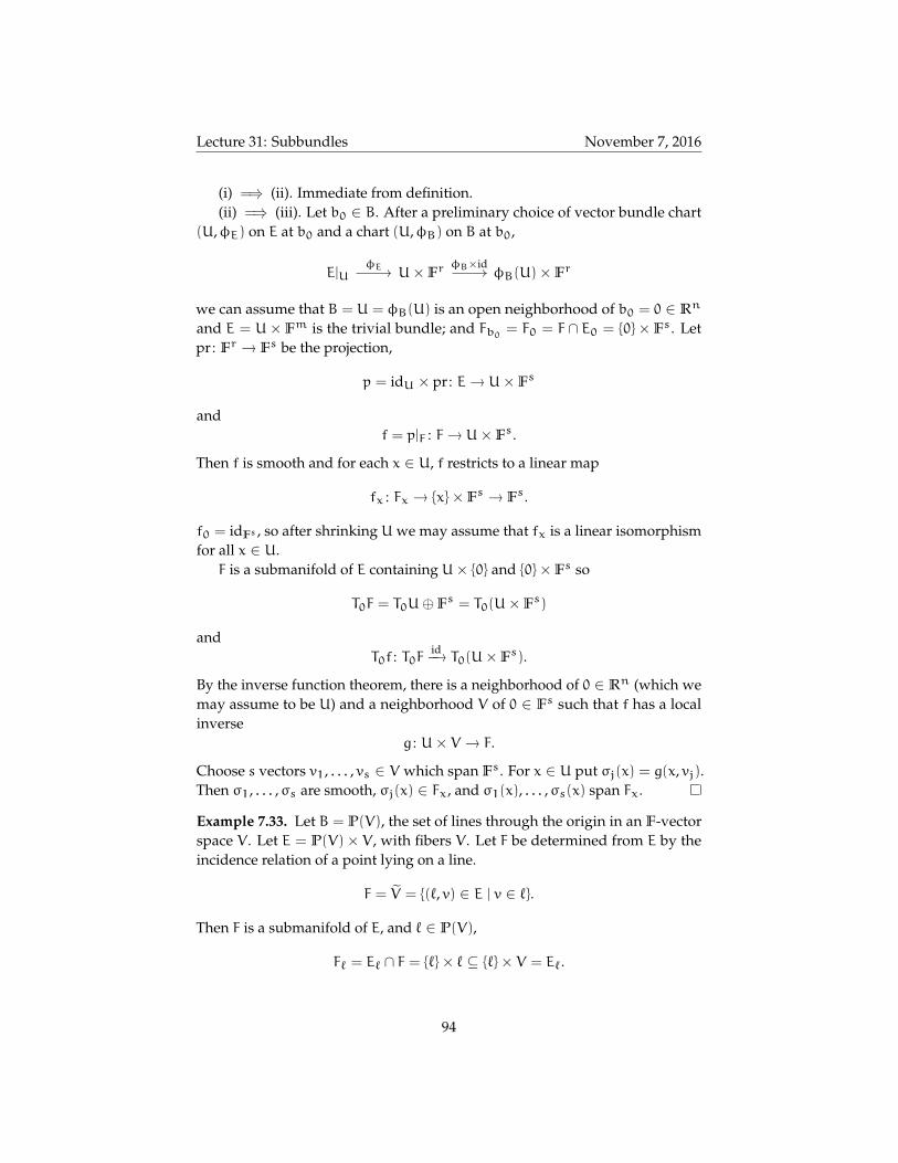
Lecture 31: Subbundles November 7, 2016
(i) =⇒ (ii). Immediate from definition.(ii) =⇒ (iii). Let b0 ∈ B. After a preliminary choice of vector bundle chart
(U,φE) on E at b0 and a chart (U,φB) on B at b0,
E|U U×Fr φB(U)×FrφE φB×id
we can assume that B = U = φB(U) is an open neighborhood of b0 = 0 ∈ Rn
and E = U× Fm is the trivial bundle; and Fb0 = F0 = F ∩ E0 = 0× Fs. Letpr : Fr → Fs be the projection,
p = idU × pr : E→ U×Fs
andf = p|F : F→ U×Fs.
Then f is smooth and for each x ∈ U, f restricts to a linear map
fx : Fx → x×Fs → Fs.
f0 = idFs , so after shrinking Uwe may assume that fx is a linear isomorphismfor all x ∈ U.F is a submanifold of E containing U× 0 and 0×Fs so
T0F = T0U⊕Fs = T0(U×Fs)
andT0f : T0F
id−→ T0(U×Fs).
By the inverse function theorem, there is a neighborhood of 0 ∈ Rn (which wemay assume to be U) and a neighborhood V of 0 ∈ Fs such that f has a localinverse
g : U× V → F.
Choose s vectors v1, . . . , vs ∈ V which span Fs. For x ∈ U put σj(x) = g(x, vj).Then σ1, . . . ,σs are smooth, σj(x) ∈ Fx, and σ1(x), . . . ,σs(x) span Fx.
Example 7.33. Let B = P(V), the set of lines through the origin in an F-vectorspace V . Let E = P(V)× V , with fibers V . Let F be determined from E by theincidence relation of a point lying on a line.
F = V = (`, v) ∈ E | v ∈ `.
Then F is a submanifold of E, and ` ∈ P(V),
F` = E` ∩ F = `× ` ⊆ `× V = E`.
94

Lecture 32: Foliations November 9, 2016
Then by Proposition 7.32(iii), this is the tautological bundle over P(V).
V
P(V) V
π β
where π is the F-line bundle projection and β is the blow-down map.
8 Foliations
Definition 8.1. Let M be a manifold. A tangent sub-bundle or distributionoverM is a subbundle of TM.
Example 8.2.
(1) Let (ξ1, . . . , ξr) be an r-frame on M, with r ≤ n = dimM. Let E be thespan of ξ1, . . . , ξr, that is,
Ex = spanξ1(x), . . . , ξr(x) ⊆ TxM
for any x ∈M. By the proposition, E is a distribution onM.
(2) Let f : M→ N be a map of constant rank. Let E = ker(Tf), that is,
Ex = ker(Txf)
for x ∈ M. For all x ∈ M, the subspace Ex ⊆ TxM has dimensiondim(M) − r. Choosing charts, (U,φ) onM, (V ,ψ) on N such that
f(x) = (x1, . . . , xr, 0, . . . , 0)
we see that the tangent chart (TU, Tφ) also defines a subbundle chart forE = ker(Tf). So E is a tangent subbundle.
Let Gr(r, Rn) be the Grassmannian of r-planes in Rn.
Definition 8.3. Let E be a subbundle of rank r of the trivial rank n bundleB×Rn. The Gauss map of E is the map f : B→ Gr(r, Rn) defined by f(b) = Eb.
Definition 8.4. Fr(r, Rn) is the Stiefel manifold of all r-frames in Rn.
Lemma 8.5. f is smooth.
95
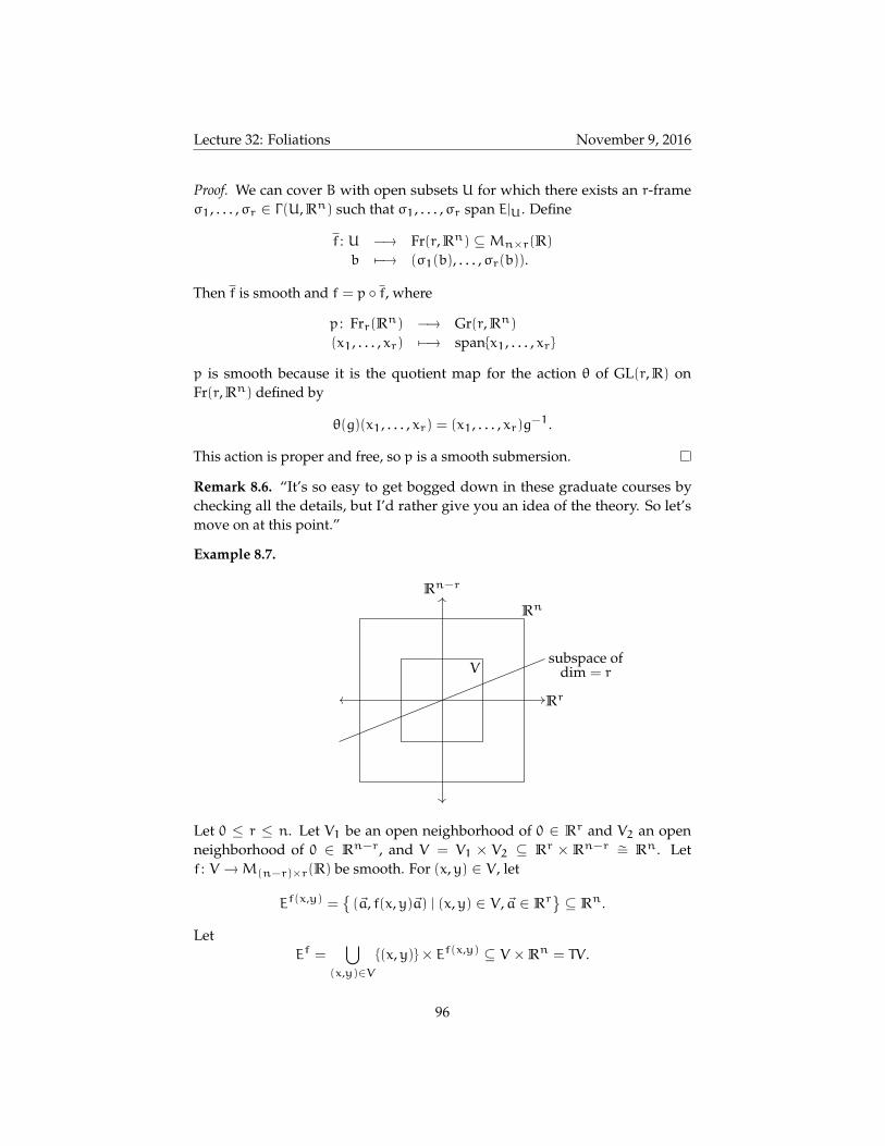
Lecture 32: Foliations November 9, 2016
Proof. We can cover B with open subsets U for which there exists an r-frameσ1, . . . ,σr ∈ Γ(U, Rn) such that σ1, . . . ,σr span E|U. Define
f : U −→ Fr(r, Rn) ⊆Mn×r(R)
b 7−→ (σ1(b), . . . ,σr(b)).
Then f is smooth and f = p f, where
p : Frr(Rn) −→ Gr(r, Rn)
(x1, . . . , xr) 7−→ spanx1, . . . , xr
p is smooth because it is the quotient map for the action θ of GL(r, R) onFr(r, Rn) defined by
θ(g)(x1, . . . , xr) = (x1, . . . , xr)g−1.
This action is proper and free, so p is a smooth submersion.
Remark 8.6. “It’s so easy to get bogged down in these graduate courses bychecking all the details, but I’d rather give you an idea of the theory. So let’smove on at this point.”
Example 8.7.
Rr
Rn−r
V
Rn
subspace ofdim = r
Let 0 ≤ r ≤ n. Let V1 be an open neighborhood of 0 ∈ Rr and V2 an openneighborhood of 0 ∈ Rn−r, and V = V1 × V2 ⊆ Rr × Rn−r ∼= Rn. Letf : V →M(n−r)×r(R) be smooth. For (x,y) ∈ V , let
Ef(x,y) =(~a, f(x,y)~a) | (x,y) ∈ V , ~a ∈ Rr
⊆ Rn.
LetEf =
⋃(x,y)∈V
(x,y)× Ef(x,y) ⊆ V ×Rn = TV .
96

Lecture 32: Foliations November 9, 2016
This is the tangent subbundle on V of rank r. Ef has a global frame: let
∂i =∂
∂xi
be the standard vector fields corresponding to the standard basis vectors e1, . . . , en ∈Rn. So a basis of Ef(x,y) is
(ei, f(x,y)ei) i = 1, . . . , r.
So the vector fields
ξi(x,y) = (∂i, f(x,y)∂i) i = 1, . . . , r
form an r-frame that spans Ef.Let πi : V → Vi be the projection for i = 1, 2. The first component of ξi is ∂i,
that is, ξi ∼π1 ∂i. Therefore,
[ξi, ξj] ∼π1 [∂i,∂j] = 0
that isT(x,y)π1[ξi, ξj](x,y) = 0.
Also, if f(0, 0) = 0, then Ef(0,0) = Rr and
ξi(0, 0) = (∂i, 0)
is just the first r standard basis vectors of Rn.
This example is important because any distribution (tangent subbundle)locally looks like the one above.
Proposition 8.8. Let E be a tangent subbundle of rank r over M. For everya ∈M, there is a chart (U,φ : U→ Rn) centered at a and a smooth
f : φ(U)→M(n−r)×r(R)
such that f(0) = 0 and E|U = (Tφ)−1(Ef).
Proof. Choose a basis v1, v2, . . . , vn ∈ TaM such that Ea = Spanv1, . . . , vr. Letα1, . . . ,αn ∈ T ∗aM. Then
daφ : TaM→ Rn
maps Ea → Rr ⊆ Rn. LetF = (Tφ)(E|U ′),
a subbundle of TV ′ = V ′ ×Rn where V ′ = φ(U ′). Let f ′ : V ′ → Gr(r, Rn) bethe Gauss map of F.
On Gr(r, Rn), we have a chart (O,ψ), centered at the standard hyperplaneRr, with ψ : O→M(n−r)×r. Let V = (f ′)−1(0) and U = φ−1(V), and f = f ′|V .Then F = Ef.
97

Lecture 33: Foliations November 11, 2016
Definition 8.9. An integral manifold of a distribution E ⊆ TM is an immersedsubmanifold A ⊆M such that TaA = Ea for all a ∈ A.
Picture E as a series of lines at each point on the manifold M, and A as a setof curves that are tangent to these lines everywhere.
Example 8.10.
(1) If E = Spanξ, ξa 6= 0 for all a, then integral manifolds are imagesof trajectories γ : I → M. Because ξ is nowhere zero, γ is an injectiveimmersion.
(2) E = ker(Tf) where f : M→ N is any constant rank map. The fibers f−1(y)are integral manifolds.
Example 8.11. E = Ef for some smooth f : V → M(n−r)×r(R), where V =
V1 × V2 ⊆ Rr × Rn−r ∼= Rn is open is a product of open sets V1 ⊆ Rr,V2 ⊆ Rn−r. Ef is the tangent subbundle over V given by
Ef(x,y) = graph of f(x,y) : Rr → Rn−r ⊆ Rn.
V1
V2
U1
U2
A
For every (x0,y0) ∈ V1 × V2, and every integral manifold A of E containing(x0,y0), by the implicit function theorem, there are open U1 ⊆ V1, U2 ⊆ V2such that A∩U is the graph of a unique smooth function u : U1 → U2.
Conversely, suppose that u : V1 → V2 is a C∞ map. Then
Au = graph of u ⊆ V1 × V2 = V
is an n-dimensional submanifold of V . Then is Au an integral submanifold?Au is the image of an embedding
u : V1 → V u(x) =
[x
u(x)
].
98

Lecture 33: Foliations November 11, 2016
Let (x,y) ∈ Au, that is y = u(x). A basis of T(x,y)Au is
Du(x)ei =
[Ir
Du(x)
]ei =
[ei
Du(x)ei
].
A basis of Ef(x,y) are the columns of[Ir
f(x,y)
].
That is, the vectors [ei
f(x,y)ei
], i = 1, . . . , r.
We want T(x,y)Au = Ef(x,y) in order for this to be integral. That is,
Du(x)ei = f(x,y)ei, i = 1, . . . , r.
Or more concisely,Du(x) = f(x,y).
We have determined the following.
Proposition 8.12. Au is an integral submanifold if and only if u satisfies thesystem of first-order partial differential equations
Du(x) = f(x,u(x)). (17)
The next theorem tells us that we cannot have integral submanifolds thatmeet in a point or anything like that.
Theorem 8.13. Let A1,A2 be integral manifolds of E. Then A1 ∩A2 is an opensubmanifold of A1 and A2.
Proof. Let E ⊆ TM be a distribution. Let a ∈ A1 ∩A2. Without loss of generality,M = V = V1 × V2, where V1 ⊆ Rr, V2 = Vn−r are open neighborhoods of 0,and a = (0, 0) ∈ Rr ×Rn−r = Rn, E = Ef for some
f : V →M(n−r)×r(R),
and A1 = graph(u1), A2 = graph(u2) for two solutions u1,u2 : V1 → V2 ofthe PDE (17).
We have that u1(0) = 0 = u2(0). Without loss, we may assume that V1 isconnected. Let x ∈ V1. Then choose a smooth path
γ : [0, 1] V1 V2u1
u2
99

Lecture 34: Integrability November 14, 2016
with γ(0) = 0 ∈ Rr, γ(1) = x. Put vi = ui γ for i = 1, 2. Then vi satisfies anODE
v ′i(t) = Dui(γ(t))γ′(t)
(17)= f(γ(t),ui(γ(t)))γ ′(t) = f(γ(t), vi(t))γ ′(t)
for 0 ≤ t ≤ 1.We have v1(0) = 0 = v2(0). Hence, by uniqueness of ODE solutions, v1 = v2.
In particular, v1(1) = v2(1), which means that
u1(x) = u2(x)
for all x ∈ V1. Therefore, u1 = u2, and it follows that A1 = A2.The theorem follows because we reduced to the case of successively smaller
neighborhoods; we have shown that on a sufficiently small open neighborhood,A1 = A2.
Corollary 8.14. Let Aii∈I be a family of integral manifolds of E. Then⋃i∈IAi
is an integral manifold as well. Moreover, if I is finite, then⋂i∈IAi is an integral
manifold of E.
8.1 Integrability
Definition 8.15. E is integrable if for every a ∈M, there is an integral manifoldof E containing a.
The union of all connected integral manifolds containing a is the uniquelargest connected integral manifold of E containing a, and is called the leaf of a.
SoM is a disjoint union of leaves. Each leaf is an r-dimensional immersedsubmanifold.
Remark 8.16 (Caution!). Let Aii∈I be a family of integral manifolds of E. LetA =
⋃i∈IAi; the topology on A may be finer than the subspace topology
inherited fromM.
Example 8.17. Let M = R3 with coordinates (x1, x2,y). Let E be the vectorbundle spanned by
ξ =∂
∂x1+ f(x1, x2)
∂
∂y,
η =∂
∂x2+ g(x1, x2)
∂
∂y,
where f,g : R2 → R are smooth. That is, for x ∈ R3,
Ex = Span
1
0
f(x1, x2)
,
0
1
g(x1, x2)
.
100
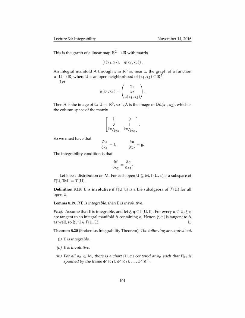
Lecture 34: Integrability November 14, 2016
This is the graph of a linear map R2 → R with matrix(f(x1, x2), g(x1, x2)
).
An integral manifold A through x in R3 is, near x, the graph of a functionu : U→ R, where U is an open neighborhood of (x1, x2) ∈ R2.
Let
u(x1, x2) =
x1x2
u(x1, x2)
.
Then A is the image of u : U→ R3, so TxA is the image of Du(x1, x2), which isthe column space of the matrix 1 0
0 1∂u/∂x1
∂u/∂x2
.
So we must have that∂u
∂x1= f,
∂u
∂x2= g.
The integrability condition is that
∂f
∂x2=∂g
∂x1.
Let E be a distribution on M. For each open U ⊆M, Γ(U,E) is a subspace ofΓ(U, TM) = T (U).
Definition 8.18. E is involutive if Γ(U,E) is a Lie subalgebra of T (U) for allopen U.
Lemma 8.19. If E is integrable, then E is involutive.
Proof. Assume that E is integrable, and let ξ,η ∈ Γ(U,E). For every a ∈ U, ξ,ηare tangent to an integral manifold A containing a. Hence, [ξ,η] is tangent to Aas well, so [ξ,η] ∈ Γ(U,E).
Theorem 8.20 (Frobenius Integrability Theorem). The following are equivalent.
(i) E is integrable.
(ii) E is involutive.
(iii) For all a0 ∈ M, there is a chart (U,φ) centered at a0 such that E|U isspanned by the frame φ∗(∂1),φ∗(∂2), . . . ,φ∗(∂r).
101

Lecture 34: Integrability November 14, 2016
Remark 8.21. Knowing (iii), we see that the submanifolds
φr+1(x) = c1, φr+2(x) = c2, · · · φn(x) = cn−r
are integral submanifolds of E|U.
Proof of Theorem 8.20.(i) =⇒ (ii). This is proven in Remark 8.21.(ii) =⇒ (iii). Let a0 ∈ M. Without loss of generality, assume M = V =
V1 × V2, where V1 is an open neighborhood of 0 ∈ Rr and V2 is an openneighborhood of 0 ∈ Rn−r, a = (0, 0), E = Ef for some smooth f : V →M(n−r)×r(R).Ef has a global frame
ξi =
(∂i
f(x,y)∂i
), i = 1, . . . , r.
and ξi ∼π1 ∂i, where π1 : Rn → Rr. That is,
Tπ1(ξi) = ∂i.
SoTπ1([ξi, ξj]) = [∂i,∂j] = 0.
We know that Γ(E) is a Lie subalgebra of T (M), so [ξi, ξj] ∈ Γ(E), which means
[ξi, ξj](x,y) ∈ E(x,y) = Ef(x,y)
for all (x,y) ∈ V1 × V2. Now
Tπ1 : Ef(x,y)
∼=−→ TxV1 ∼= Rr.
Therefore, [ξi, ξj](x,y) = 0 for all (x,y) ∈ V , so
[ξi, ξj] = 0.
Then by Proposition 8.8 and Example 8.7, there is a chart (U,φ) centered ata0 ∈Mwith ξi = φ∗(∂i).
(iii) =⇒ (i). By Remark 8.21, above, there is an integral submanifold throughevery point inM. So E is integrable.
Fact 8.22. IfM is paracompact, then the leaves of an integrable distribution arealso paracompact.
102

Lecture 35: Operations on Vector Bundles November 16, 2016
8.2 Distributions on Lie Groups.
LetM = G be a Lie group.
Definition 8.23. A vector field ξ ∈ T (G) is left-invariant if TLg(ξh) = ξgh forall g ∈ G. Write T (G)L for the space of all left-invariant vector fields.
So this vector field is determined by it’s value in the Lie algebra g = TidG.Recall that the left trivialization
φL : G× g −→ TG
(g, ξ) 7−→ TidLg(ξ)
is a diffeomorphism. For ξ ∈ g, let ξL,g = φL(g, ξ). Then ξL ∈ T (G)L. There isa one-to-one correspondence
g = TidG←→ T (G)L.
Lemma 8.24. T (G)L is a Lie subalgebra of T (G).
Proof. ξ,η ∈ T (G)L =⇒ L∗g([ξ,η]) = [L∗g(ξ),L∗g(η)] = [ξ,η] for all g ∈ G.
Via the isomorphism φL : g→ T (G)L, this makes g = TidG a Lie algebra.
Definition 8.25. g is the Lie algebra of G.
Remark 8.26. If we had done this with right-invariant vector fields instead, wewould end up with the opposite Lie algebra gop, which is the same except thebracket has a negative sign.
9 Differential Forms
9.1 Operations on Vector Bundles
Let π : E → B be a smooth vector bundle over F = R, C. We want to performalgebraic operations on the fibers of E.
Example 9.1. E∗ is the dual of E. Define
E∗ =⊔b∈B
(Eb)∗
where E∗b = HomF(Eb, F) is the dual vector space. Define π = πE∗ : E∗ → B by
sending (Eb)∗ to b. To get a vector bundle atlas on E∗, take a chart (U,φ) for E:
E|U U×Fr
U.
φ
pr1
103

Lecture 35: Operations on Vector Bundles November 16, 2016
We have F-linear isomorphisms
Eb b×Fr Fr
φb
φ
We have transpose maps φTb : (Fr)∗ ∼= (Eb)
∗. Define a chart (U,φ∗) on E∗
E∗|U U× (Fr)∗
U
φ∗
πpr1
by letting the restriction of φ∗ be the inverse transpose map
(φTb)−1 : E∗b
∼= (Fr)∗ ∼= b× (Fr)∗.
To verify that this is an atlas, we need to check compatibility. Given twocharts (U1,φ1) and (U2,φ2) on Ewith transition map g12 : U1∩U2 → GL(r, F),where g12(b) = φ2,b φ−1
1,b. The transition map for (U1,φ∗1) and (U2,φ∗2) is
g∗12(b) = (φT2,b)−1 (φT1,b)
−1 = (g12(b)T )−1.
That is,U1 ∩U2 GL(r, F)
GL(r, F)
g∗12
g12
f
g∗12 = f g12, where f(A) = (AT )−1. In particular, the transition map g∗12 =
f g12 is smooth since f is a Lie group homomorphism, and therefore the dualcharts define an atlas. Hence E∗ is a vector bundle.
If σ1, . . . ,σr is an r-frame on E|U corresponding to a chart (U,φ) on E, thentake the r-frame on E∗|U corresponding to (U,φ∗) is the dual frame σ∗1, . . . ,σ∗r ∈Γ(U,E∗) characterized by
σ∗i(σj) = δij,
that is,σ∗1(b)(σj(b)) = δij
for all b ∈ U.
Example 9.2. A special case of the previous example is when E = TM is thetangent bundle of a manifoldM. Then E∗ = T ∗M is the cotangent bundleof M.Choosing a chart (U,φ) onM gives rise to an n-frame on TU
∂
∂x1,∂
∂x2, . . . ,
∂
∂xn.
104

Lecture 35: Operations on Vector Bundles November 16, 2016
The dual frame on T ∗U is denoted by
dx1,dx2, . . . ,dxn.
Definition 9.3. Sections of T ∗M are called differential forms of degree 1.
For a more general construction of new vector bundles from old ones, let Vectbe the category of finite-dimensional vector spaces over F. Let F : Vect→ Vectbe a functor.
For a vector bundle π : E→ B, define
F(E) =∐b∈BF(Eb)
as a set, and define π : F(E)→ B by sending F(Eb) to b ∈ B.A chart (U,φ) on E gives rise to a chart (U,F(φ)) on F(E) as follows.
F(E)|U U×F(Fr)
U
F(φ)
pr1
For each b ∈ U, we have φb : Eb ∼= Fr.If F is covariant, then apply F :
F(φb) : F(Eb) ∼= F(Fr).
Define the restriction of F(φ) to F(Eb) to be the map
F(Eb) F(Fr) b×F(Fr)F(φb)
If F is contravariant, then apply F to φb to get
F(φb) : F(Fr) ∼= F(Eb).
Define the restriction of F(φ) to F(Eb) to be the map
F(Eb) F(Fr) b×F(Fr)F(φb)−1
To check compatibility of the charts, suppose (U1,φ1) and (U2,φ2) arecharts on Ewith transition
g12 : U1 ∩U2 −→ GL(r, F).
Then the charts (U1,F(φ1)) and (U2,F(φ2)) have transition map
F(g12) : U12 → GL(F(Fr))
105

Lecture 36: Alternating algebras November 18, 2016
given by eitherF(g12)(b) = F(g12(b))
in the covariant case, or
F(g12)(b) = F(g12(b))−1
in the contravariant case. We need this to be smooth for the charts to be compat-ible. But F defines a map
Hom(Fr, Fr)F−→ Hom(F(Fr),F(Fr)),
which restricts to a map
GL(r, F)F−→ GL(F(Fr)), (18)
which is a homomorphism if F is covariant and an antihomomorphism if F iscontravariant.
Theorem 9.4. Suppose that F has the property that (18) is smooth. Then F(E)is a smooth vector bundle over B, and if gij : Uij → GL(r, F) | i, j ∈ I is acocycle representing E, then a cocycle for F(E) is
F(gij) : Uij → GL(F(Fr)).
Example 9.5. If F = (−)∗ is the dual functor, then we obtain the dual vectorbundle. Similarly, we could let F be the tensor algebra, symmetric algebra, oralternating algebra over a vector space V , giving other bundles.
9.2 Alternating algebras
Definition 9.6. Let Vect be the category of finite-dimensional vector spaces andlinear maps over the field F = R, C. A covariant functor F : Vect → Vect issmooth if for all objects V ,W,
Hom(V ,W)F−→ Hom(F(V), F(W))
is smooth. Similarly for contravariant functors.
A smooth functor F can be applied to the fibers of a vector bundle E→ B toyield a new vector bundle F(E)→ B.
Example 9.7. Let F(V) = V∗, F(f : V →W) = (fT : W∗ → V∗). The map
Hom(V ,W)F
−−−−−−→transpose
Hom(V∗,W∗)
is smooth because it’s linear.
106

Lecture 36: Alternating algebras November 18, 2016
Let k be a commutative ring and V a k-module. For example, k = R,V = TxM, or k = C∞(M), V = T (M).
Definition 9.8. The alternating algebra of V is the k-module A(V) spanned byall symbols
u1 ∧ u2 ∧ . . .∧ un
for n ∈N, u1, . . . ,un ∈ V . These are subject to all relations of the form:
u1 ∧ . . .∧ (aui + a′ui ′)∧ . . .∧ un = a(u1 ∧ . . .∧ ui ∧ . . .∧ un)
+ a ′(u1 ∧ . . .∧ ui ′ ∧ . . .∧ un)(19)
u1 ∧ . . .∧ ui ∧ . . .∧ uj ∧ . . .∧ uk = 0 if ui = uj for i 6= j. (20)
for all a,a ′ ∈ k and ui ∈ V . If n = 0, we interpret u1 ∧ . . .∧ un as 1 ∈ k.A(V) is an associative algebra over kwith unit and multiplication ∧ defined
on generators by
(u1 ∧ . . .∧ un)∧ (v1 ∧ . . .∧ vm) = u1 ∧ . . .∧ un ∧ v1 ∧ . . .∧ vm.
Axiom (19) is called multilinarity and axiom (20) is called alternating.
Example 9.9. 5+ 3u+ v∧w ∈ A(v) for any u, v,w ∈ V .
Example 9.10. u∧ v = −(v∧ u) for all u, v ∈ V . Why?
(u+ v)∧ (u+ v) = 0
Then apply the multilinearity and alternating relations above.
Definition 9.11. Some variations on Definition 9.8.
(a) If we omit (20), the resulting algebra is the tensor algebra T(V) withmultiplication denoted ⊗.
(b) If we replace (20) by the following relation
u1u2 · · ·ui · · ·uj · · ·un = u1u2 · · ·uj · · ·ui · · ·un,
we obtain the symmetric algebra S(V) of V with multiplication denotedby juxtaposition.
(c) If we replace (20) with the Clifford Axiom,
uu = q(u),
where q : V → k is a quadratic form, we get the Clifford algebra Cl(V ,q)of the pair (V ,q).
107
Lecture 36: Alternating algebras November 18, 2016
Definition 9.12. An element of A(V) has degree n if it’s a linear combinationof generators u1 ∧ . . .∧ un, with ui ∈ V . The elements of degree n form ak-submodule, the n-th alternating power An(V) of V .
We have that
A(V) =∞⊕n=0
An(V)
where A0(V) = k, A1(V) = V . Therefore, A(V) is a graded algebra, with
Ai(V)∧Aj(V) ⊆ Ai+j(V).
Remark 9.13. If x ∈ Ai(V),y ∈ Aj(V), then y∧ x = (−1)ij(x∧ y).
Definition 9.14. The graded commutator is given on basis elements x ∈ Ai(V),y ∈ Aj(V) by
[x,y] = x∧ y− (−1)ij(y∧ x)
and extended by linearity. This is also called the Koszul sign rule.
By Remark 9.13, A(V) is graded commutative: [x,y] = 0 for all x,y ∈ A(V).The alternating algebra construction V 7→ A(V) defines a functor
A : Modk → Algk,
where Modk is the category of k-modules and Algk is the category of k-algebras.If V ,W are modules and f : V →W is k-linear, then define
A(f) : A(V)→ A(W)
on generators by
A(f)(u1 ∧ . . .∧ un) = f(u1)∧ . . .∧ f(un),
and extend by k-lienarity.This is then well-defined, k-linear and moreover multiplicative (which
means that A(f)(x ∧ y) = A(f)(x) ∧ A(f)(y) for all x,y). We also say thatA(f) is of degree zero, that is,
deg(A(f)(x)) = deg(x).
Therefore, A(f) is a homomorphism of graded algebras.
Some questions we may ask are: what does a basis ofA(V) look like? What’sthe matrix of a linear transformation A(f) relative to the matrix for f?
Let V∗ = Homk(V ,k) be the k-dual of V . Define a pairing
Ak(V∗)×Ak(V)→ k
108

Lecture 37: Alternating algebras November 21, 2016
by
(φ1 ∧ . . .∧φk)(u1 ∧ . . .∧ uk) = det
φ1(u1) . . . φ1(uk)...
. . ....
φk(uk) . . . φk(uk)
for φi ∈ V∗, ui ∈ V . This is well-defined and k-bilinear.
Now assume that V is a free k-module of finite rank n. Choose a basisb1, . . . ,bn of V , with dual basis b∗1, . . . b∗n such that b∗i(bj) = δij. Let I =
(i1, . . . , in) be a multi-index with 1 ≤ i` ≤ r. Write
bI = bi1 ∧ . . .∧ bir and b∗I = b∗i1
∧ . . .∧ b∗ir .
We say that I is increasing if 1 ≤ i1 < . . . < ir ≤ n. Let Inr be the set of suchmulti-indices.
Lemma 9.15. The elements bI for I ∈ Inr span Ak(V). Likewise, the elementsb∗I span Ak(V∗).
Proof. Let u1, . . . ,uk ∈ V . Then it’s enough to show that u1 ∧ . . .∧ uk is alinear combination of the bI. Expressing
ui =∑
cijbi
with cij ∈ k and using the properties of the wedge product, we see that
u1 ∧ . . .∧ uk =
k∑j1,j2,...,jk=1
c1j1c2j2 · · · ckjkbj1 ∧ . . .∧ bjk .
Using the alternating rule, we may rearrange this to be in the form
u1 ∧ . . .∧ uk =∑J∈Ink
aJbJ.
Lemma 9.16. b∗I(bJ) = δI,J for all I, J ∈ Ink .
Proof.
b∗I(bJ) = (b∗i1 ∧ . . .∧ b∗ik)(bj1 ∧ . . .∧ bjk)
= det
b∗i1(bj1) · · · b∗i1(bjk)
.... . .
...b∗ik(bj1) · · · b∗ik(bjk)
= det(δip,jq)1≤p,q≤k)
=
1 I = J
0 I 6= J
109

Lecture 37: Differential Forms November 21, 2016
Theorem 9.17. Suppose that V is a free k-module of rank nwith basis b1, . . . ,bn.
(i) The collections bI | I ∈ Ink and b∗I | I ∈ Ink are bases of the k-modulesAk(V) and Ak(V∗), respectively. In particular, these modules are free ofrank #Ink =
(nk
). Also, Ak(V) = Ak(V∗) = 0 for k > n.
(ii) The pairing Ak(V∗)×Ak(V)→ k is nondegenerate in the sense that theassociated map Ak(V∗)→ Ak(V)∗ is an isomorphism.
(iii) As a k-module, A(V) is free of rank∑nk=0
(nk
)= 2n.
Now let V ,W be free k-modules and f : V →W a linear map. Choose basesb1, . . . ,bn of V and c1, . . . , cm of W. Let (fij) ∈ Mm×n(k) be the matrix of f,that is,
fij = c∗i(f(bj)) ∈ k.
Recall that f : V →W induces a k-linear map Ak(f) : Ak(V)→ Ak(W) given by
Ak(f)(u1 ∧ . . .∧ uk) = f(u1)∧ . . .∧ f(uk).
Theorem 9.18. The matrix elements of Ak(f) relative to the bases bJ | J ∈ Ink and cI | I ∈ Imk are det(fI,J), where fI,J ∈ Mk×k(k) is the k× k submatrix(fip,jq)1≤p,q≤k with rows i1, . . . , ik and columns j1, . . . , jk.
Proof.
c∗I(Ak(f)(bJ)) = (c∗i1 ∧ . . .∧ c
∗ik)(f(bj1)∧ . . .∧ f(bjk))
= det(c∗ip(f(bjq)))1≤p,q≤k
= det(fip,jq)1≤p,q≤k
= det(fI,J)
9.3 Differential Forms
Now set k = R and let VectR be the category of finite-dimensional R-vectorspaces.
Corollary 9.19. The functors Ak : VectR → VectR are smooth.
Proof. For all V ,W in VectR,
Mm×n(R) ∼= HomR(V ,W)Ak−−→ HomR(A
k(V),Ak(W) ∼=M(mk )×(nk)(R)
is smooth, and in fact multilinear.
110

Lecture 38: Differential Forms November 28, 2016
So for for every smooth vector bundle π : E→ B, with cocyles gij we geta new vector bundles Ak(E)→ B and Ak(E∗)→ Bwith cocycles Ak(gij andAk(g∗ij), respectively.
We also have an alternating algebra bundle
A(E) =n⊕k=0
Ak(E),
and an isomorphism Ak(E∗) ∼= Ak(E)∗.
Definition 9.20. In the special case that E = T ∗M for a manifoldM, we say thatA(T ∗M) is the bundle of differential forms onM, and use the notation
Ω(M) =n⊕k=0
Ωk(M).
Definition 9.21. When E = TM for a manifold M, we say that A(TM) is thebundle of multivector fields onM and use the notation
X (M) =n⊕k=0
X k(M).
Definition 9.22. Let Vk = V × V × . . .× V and letW be any other k-module. Amap µ : Vk →W is alternating multilinear if
(a) µ(u1, . . . ,ui, . . . ,uj, . . . ,uk) = 0 if ui = uj for some i 6= j.
(b) ui 7→ µ(u1, . . . ,ui, . . . ,uk) is linear for all i.
Then put
Altk(V ,W) = µ : Vk →W | µ is alternating and multilinear,
and also Altk(V) = Altk(V ,k).
Example 9.23. If V = kn, then µ = det : Vn → k is an element of Altn(V).Furthermore, for any V , we may define i : Vn → An(V) by i(u1, . . . ,uk) =
u1 ∧ . . .∧ uk. Then i is alternating multilinear.
Theorem 9.24 (The universal property of Ak(V)). For every alternating multi-linear µ : Vk →W, there is a unique linear µ : Ak(V)→W satisfying µ = µ i.
Vk W
Ak(V)
i
µ
∃!µ
111

Lecture 38: Differential Forms November 28, 2016
Proof. Supposing that µ exists, there’s only one possible way to define it: wehave
µ(u1, . . . ,uk) = µ(i(u1, . . . ,uk)) = µ(u1 ∧ . . .∧ uk).
Since the products u1 ∧ . . .∧ uk generate Ak(V), this shows that µ is unique.Now define µ on generators by µ(u1 ∧ . . .∧ uk) = µ(u1,u2, . . . ,uk). This
is well-defined because µ is alternating multilinear. So µ is a k-linear mapAk(V)→W and µ = µ i.
Corollary 9.25. Altk(V ,W) ∼= Homk(Ak(V),W).
Proof. The isomorphism is given by µ 7→ µ i.
Example 9.26. A special case of this is whenW = k, when
Altk(V) ∼= Ak(V)∗ ∼= Ak(V∗)
Fact 9.27. Let π : E→ B be a vector bundle.
(i) Γ(E∗) ∼= Γ(E)∗
(ii) Γ(Ak(E)) ∼= Ak(Γ(E))
Proof Sketch. Recall that Γ(E) is the space of smooth sections B→ E of E. Γ(E) isa module over C∞(B).
In (i), E∗ =⊔b∈B E
∗b is the dual vector bundle with fibers E∗b = HomR(Eb, R),
while Γ(E)∗ = HomC∞(B)(Γ(E),C∞(B)) is the dual C∞(B)-module of Γ(E). Therest of this will be on the homework.
In (ii), Ak(E) =⊔b∈BA
kR(Eb) is the k-th alternating power of E, while
Ak(Γ(E)) = AkC∞(B)(Γ(E)) is the k-th alternating power of the C∞(B)-module
Γ(E).
We can put this previous fact together with the definition of the bundle ofdifferential forms onM to see that
Ωk(M) := Γ(Ak(T ∗M)) ∼= Γ(Ak(TM)∗)
∼= Γ(Ak(TM))∗ Fact 9.27(i)∼= Ak(Γ(TM))∗ Fact 9.27(ii)∼= Ak(T (M))∗
∼= Altk(T (M))
We have proved
Proposition 9.28.Ωk(M) ∼= Altk(T (M)).
112

Lecture 38: The de Rahm complex November 28, 2016
Figure 1: An octopus eating vector fields. (Illustration by Lila Greco)
Remark 9.29. A k-form on the manifoldM is like an octopus that eats k-manyvectors ξ1, . . . , ξk onM and spits out a real number. The expression of a k-formin a chart (U,φ) onM is as follows. Let α ∈ Ωk(M). Let ∂/∂x1 , . . . , ∂/∂xn be theframe on TU defined by φ, and dx1, . . . ,dxn the dual frame of T ∗U. For I ∈ Ink ,put
dxI = dxi1 ∧ . . .∧ dxik .
Then there exist unique functions fI ∈ C∞(U) such that
α|U =∑I∈Ink
fIdxI,
where fI = α|U(∂/∂xi1 , . . . , ∂/∂xik ).
9.4 The de Rahm complex
Ω0(M) = Γ ∗ (A0(T ∗M)) = Γ(trivial bundleM×R) = C∞(M).
Let f ∈ Ω0(M) = C∞(M). Recall that
df = pr2 Tf : TMTf−→ TR = R×R
pr2−−→ R
For ξ ∈ T (M) we define df(ξ) = Lξ(f) by
df(ξ)(x) = dxf(ξx) ∈ R
If g ∈ C∞(M) we have
df(gξ) = Lgξ(f) = gLξ(f) = gdf(ξ).
So df, considered as a map T (M) → C∞(M) is C∞(M)-linear. So we mayregard df as a section of T ∗M,
df ∈ Γ(T ∗M) = Γ(A1(T ∗M)) = Ω1(M).
113

Lecture 39: The de Rahm complex November 30, 2016
This in turn tells us that d is a map
d : Ω0(M)→ Ω1(M).
Then d is R-linear and satisfies the Leibniz rule:
d(fg) = (df)g+ f(dg)
becauseLξ(fg) = Lξ(f)g+ fLξ(g)
for all ξ ∈ T (M).
Lemma 9.30. LetM = U open in Rn and f ∈ C∞(M). Then
df =
n∑i=1
∂f
∂xidxi.
Proof. We have that
df =
n∑i=1
gidxi
for some gi ∈ C∞(U), and these gi are given by
df
(∂
∂xi
)=∂f
∂xi.
Remark 9.31. The previous lemma tells us that in particular, d(xi) = dxi. Thisexplains the notation dxi for the 1-form dual to the vector field ∂/∂xi .
We want to expand this map d into a sequence of maps
Ω0(M)d−→ Ω1(M)
d−→ · · · d−→ Ωn(M)→ 0
satisfying the graded Leibniz rule d(α∧ β) = dα∧ β+ (−1)kα∧ dβ for α ∈Ωk(M) and β ∈ Ω`(M).
Definition 9.32. For α ∈ Ωk(M), define dα ∈ Ωk+1(M) by
dα(ξ1, . . . , ξk+1) =k+1∑`=1
(−1)`+1Lξ`(α(ξ1, . . . , ξ`, . . . , ξk+1))
+∑
1≤i<j≤n(−1)i+jα([ξi, ξj], ξ1, . . . , ξi, . . . , ξj, . . . , ξ`)
for ξ1, . . . , ξk+1 ∈ T (M).
114

Lecture 39: The de Rahm complex November 30, 2016
Example 9.33. In the special case that α = f ∈ Ω0(M) = C∞(M), then
(df)(ξ) = Lξ(f).
This coincides with the definition of d : Ω0 → Ω1.
Example 9.34. If α ∈ Ω1(M), then
(dα)(ξ,η) = Lξ(α(η)) −Lη(α(ξ)) −α([η, ξ]) (21)
Lemma 9.35. dα is alternating multilinear over C∞(M) and therefore defines a(k+ 1)-form. That is, d : Ωk → Ωk+1 is well-defined.
Proof. We only check the case when k = 1. For k = 1, α ∈ Ω1(M), so dα(ξ, ξ) =0 by (21). Moreover, (21) is additive with respect to η and ξ.
Now if f ∈ C∞(M),
dα(fξ,η) = Lfξ(α(η)) −Lη(α(fξ)) −α([fξ,η])
= fLξ(α(η)) −Lη(fα(ξ)) +α([η, fξ])
= fLξ(α(η)) − (Lη(f)α(ξ) + fLη(α(ξ))) +α(Lη(fξ)) (22)
Now
α(Lη(fξ)) = α (Lη(f)(ξ) + fLη(ξ))= Lη(f)α(ξ) + fα(Lη(ξ))= Lη(f)α(ξ) + fα([η, ξ])
= Lη(f)α(ξ) − fα([η, ξ])
Substittue this into (22) to see that
dα(fη, ξ) = f(Lξ(α(η)) −Lη(α(ξ)) −α([ξ,η])
).
Lemma 9.36. LetM = U be open in Rn, α ∈ Ωk(U),
α =∑I
fIdxI.
Then
dα =∑I
dfI ∧ dxI =∑I
n∑i=1
∂fI∂xi
dxi ∧ dxI.
Proof. Put ∂i = ∂/∂xi , and ∂I = ∂i1 ∧ . . .∧ ∂ik . Recall that fI = α(∂I). Similarly,
dα =∑J∈Ink+1
gJdxJ
115

Lecture 39: The de Rahm complex November 30, 2016
with
gJ = dα(∂J) =
k+1∑`=1
∂j`(α(∂J\j`)) + 0
=∑`
(−1)`+1∂j`fJ\j`
=∑`
(−1)`+1∂fJ\j`
∂x`
So
dα =∑J
k+1∑`=1
(−1)`+1∂fJ\j`
∂x`dxJ =
∑I
n∑i=1
∂fI∂xi
dxi ∧ dxI.
Where we substitute I = J \ j` and i = j`.
Remark 9.37. The previous proof also shows that dxJ = (−1)`+1dxi∧dxI. Thegraded Leibniz rule follows from this.
Theorem 9.38. d2 = 0, that is, d(dα) = 0 for all α ∈ Ωk(M).
Proof. Enough to show that d2α|U = 0 for every coordinate neighborhood U onM. So without loss we may assume thatM = U ⊆ Rn open, and
α =∑I
fIdxI.
Then
d(dα) = d
(∑I
∑i
∂fI∂xi
dxi ∧ dxI
)
=∑I
∑j
∑i
∂2fI∂xi∂xj
dxi ∧ dxj ∧ dxI
=∑I
∑1≤i<j≤n
(∂2fI∂xi∂xj
−∂2fI∂xj∂xi
)dxi ∧ dxj ∧ dxI
= 0
The mixed partial derivatives of fI cancel because f is smooth.
Corollary 9.39.Ω(M) =∞⊕k=0
Ωk(M) is a commutative differential graded al-
gebra.
116

Lecture 40: De Rahm Cohomology December 2, 2016
9.5 De Rahm Cohomology
Definition 9.40. A k-form α ∈ Ωk(M) is closed if dα = 0 (if α is in the kernelof d).
A k-form α ∈ Ωk(M) is exact if α = dβ for some β ∈ Ωk−1(M) (if α is inthe image of d). Set
Zk(M) = α ∈ Ωk(M) | dα = 0 = ker(d : Ωk(M)→ Ωk+1(M))
Bk(M) = dβ | β ∈ Ωk−1(M) = im(d : Ωk−1(M)→ Ωk(M))
Notice that d2 = 0 implies that Bk(M) ⊆ Zk(M).
Definition 9.41. The k-th de Rahm cohomology ofM is the R-vector space
HkDR(M) =Zk(M)/
Bk(M)
Definition 9.42. The cup product of two classes [α] ∈ HkDR(M) and [β] ∈H`DR(M) is [α]^ [β] = [α∧β] ∈ Hk+`DR (M).
The cup product is well-defined because of the following lemma.
Lemma 9.43.
(i) α,β closed =⇒ α∧β closed.
(ii) α closed and β exact =⇒ α∧β exact.
Proof.
(i) d(α∧β) = dα∧β+ (−1)k`α∧ dβ = 0
(ii) Let β = dγ. Then
d(α∧ γ) = dα∧ γ± α∧ dγ = 0∧ γ± α∧β
Therefore, α∧β is exact.
This also shows us that Z(M) =∞⊕k=0
Zk(M) is a sub-algebra of Ω(M) that
is also a commutative graded differential algebra. Similarly, B(M) is a gradedideal of Z(M).
Corollary 9.44. HDR(M) =∞⊕k=0
HkDR(M) is a commutative graded R-algebra.
117

Lecture 40: Functoriality of HDR December 2, 2016
Example 9.45.
H0DR(M) = Z0(M) = ker(d : C∞(M)→ Ω1(M))
= f ∈ C∞(M) | df = 0
= f ∈ C∞(M) | fconstant on connected components ofM
Therefore, the zeroth de Rahm cohomology of M is Rπ0(M), where π0(M) isthe set of connected components ofM.
The de Rahm cohomology algebra of M satisfies several important prop-erties. Namely, M 7→ HDR(M) is functorial, homotopy invariant, and has theMayer-Vietoris property.
9.6 Functoriality of HDRLet F : M → N be a smooth map. Recall that we have maps of smooth vectorbundles
TM
M
∗
T ∗M
M
A
A(T ∗M)
M.
F induces a map on tangent spaces.
TM TN
M N
TF
F
Let F be a contravariant functor. Then we get a pullback map on sections ofF(TX)
F∗ : Γ(F(TN))→ Γ(F(TM)).
In particular, when F = A, we get
F ∗ : Ω(N)→ Ω(M).
Example 9.46.
(a) For k = 0, f ∈ Ω0(N) = C∞(N) and F∗(f) = f F.
(b) For f ∈ Ω0(N), let α = df. Then
F∗(α)x(v) = αF(x)(TxF(v)) = dF(x)f(TxF(v)) = dx(f F)(v).
So F∗(α) = d(f F) = dF∗(f), that is, F∗(df) = dF∗(f).
118

Lecture 40: Other properties of HDR(M) December 2, 2016
Fact 9.47 (Other properties of pullback).
(a) F∗(dα) = dF∗(α) for all α ∈ Ωk(N).
(b) F∗(α∧β) = F∗(α)∧ F∗(β)
(c) If G : N→ P is smooth as well, then (G F)∗ = F∗ G∗, and we get
(G F)∗ : Ω(P)G∗−−→ Ω(N)
F∗−→ Ω(M).
So Ω is a contravariant functor from the category of Manifolds to thecategory of commutative differential graded algebras.
We also get an induced map on cohomology. F∗ induces an homomorphismof commutative graded algebras also denoted by F∗,
F∗ : HDR(N) −→ HDR(M)
[α] 7−→ [F∗(α)]
9.7 Other properties of HDR(M)
Definition 9.48. Smooth maps F0, F1 : M → N are homotopic if there is asmooth map F : M× [0, 1] → N with F(x, 0) = F0(x) and F(x, 1) = F1(x). Thenotation is Ft(x) = F(x, t).
Think ofM× [0, 1] as a manifold with boundary.
Theorem 9.49 (de Rahm). If two maps F0, F1 : M→ N are homotopic, then theyinduce the same map on cohomology, that is F∗0 = F∗1 : HDR(N)→ HDR(M).
In fact, de Rahm’s theorem can say more: it says that the de Rahm cohomol-ogy ofM is identical to the singular cohomology H(M;R) ofM as a topologicalspace.
Example 9.50. M is contractible to a point x0 ∈ M if the maps id : M → M
and the constant map f : x 7→ x0 are homotopic. Then id∗ = f∗ : HDR(M) →HDR(M). So
HDR(M) =
R k = 0
0 k > 0.
Example 9.51. HDR(M) ∼= HDR(M× [0, 1])
HDR(M) has a Mayer-Vietoris long exact sequence.
119

Lecture 40: Other properties of HDR(M) December 2, 2016
Lemma 9.52. Suppose that U,V ⊆M are open, and U∪ V =M. Then there is ashort-exact sequence
0 −→ Ω(M)f−→ Ω(U)⊕Ω(V)
g−→ Ω(U∩ V) −→ 0
α 7−→ (α|U,α|V )(β,γ) 7−→ β|U∩V − γ|U∩V
Proof sketch. The fact that g f = 0 is clear. If g(β,γ) = 0, then (β,γ) = f(α) forsome α. So im(f) = ker(g).
Injectivity of f is clear. For surjectivity of γ, use a partition of unity for thecover U,V ofM.
Theorem 9.53 (Mayer-Vietoris). There is a long exact sequence of cohomology.
· · ·→ Hk(U)→ Hk(V)→ Hk(M)→ Hk(U∩V)→ Hk+1(U)⊕Hk+1(V)→ · · ·Example 9.54. We can use the previous theorem to calculate the de Rahmcohomology of Sn, for example.
HkDR(Sn) =
R k = 0,n
0 k 6= 0,n
120