Math 5364 Notes Chapter 5: Alternative Classification Techniques Jesse Crawford Department of...
119
Math 5364 Notes Chapter 5: Alternative Classification Techniques Jesse Crawford Department of Mathematics Tarleton State University
-
Upload
nathan-mosley -
Category
Documents
-
view
221 -
download
1
Transcript of Math 5364 Notes Chapter 5: Alternative Classification Techniques Jesse Crawford Department of...

Math 5364 NotesChapter 5: Alternative Classification Techniques
Jesse Crawford
Department of MathematicsTarleton State University

Today's Topics
• The k-Nearest Neighbors Algorithm
• Methods for Standardizing Data in R
• The class package, knn, and knn.cv

k-Nearest Neighbors
• Divide data into training and test data.• For each record in the test data
• Find the k closest training records• Find the most frequently occurring
class label among them• The test record is classified into that
category• Ties are broken at random
• Example• If k = 1, classify green point as p• If k = 3, classify green point as n• If k = 2, classify green point as p
or n (chosen randomly)

k-Nearest Neighbors Algorithm
Algorithm depends on a distance metric d

Euclidean Distance Metric
1 2 1 2
1 2 1 2
2 211 21 1 2
( , )
( ) ( )
( () )p p
d x x x x
x x x x
x xx x
‖ ‖
=
1 11 1
2 21 2
( , , )
( , , )
p
p
x
x
x x
x x
Example 1• x = (percentile rank, SAT)• x1 = (90, 1300)• x2 = (85, 1200)• d(x1, x2) = 100.12
Example 2• x1 = (70, 950)• x2 = (40, 880)• d(x1, x2) = 76.16
• Euclidean distance is sensitive to measurement scales.• Need to standardize variables!

Standardizing Variables
1
1
Data set , ,
sample mean
sample standard deviation
Then , , has mean 0
and standard deviation 1
n
ii
n
x x
x
s
x xz
s
z z
mean percentile rank = 67.04st dev percentile rank = 18.61
mean SAT = 978.21st dev SAT = 132.35
Example 1• x = (percentile rank, SAT)• x1 = (90, 1300)• x2 = (85, 1200)• z1 = (1.23, 2.43)• z2 = (0.97, 1.68)• d(z1, z2) = 0.80
Example 2• x1 = (70, 950)• x2 = (40, 880)• z1 = (0.16, -0.21)• z2 = (-1.45, -0.74)• d(z1, z2) = 1.70

Standardizing iris Data
x=iris[,1:4]xbar=apply(x,2,mean)xbarMatrix=cbind(rep(1,150))%*%xbars=apply(x,2,sd)sMatrix=cbind(rep(1,150))%*%s
z=(x-xbarMatrix)/sMatrixapply(z,2,mean)apply(z,2,sd)
plot(z[,3:4],col=iris$Species)

Another Way to Split Data
#Split iris into 70% training and 30% test data.set.seed=5364train=sample(nrow(z),nrow(z)*.7)
z[train,] #This is the training dataz[-train,] #This is the test data

The class Package and knn Function
library(class)
Species=iris$SpeciespredSpecies=knn(train=z[train,],test=z[-train,],cl=Species[train],k=3)
confmatrix(Species[-train],predSpecies)
Accuracy = 93.33%

Leave-one-out CV with knn
predSpecies=knn.cv(train=z,cl=Species,k=3)confmatrix(Species,predSpecies)
CV estimate for accuracy is 94.67%

Optimizing k with knn.cv
accvect=1:10
for(k in 1:10){ predSpecies=knn.cv(train=z,cl=Species,k=k) accvect[k]=confmatrix(Species,predSpecies)$accuracy}
which.max(accvect)
For binary classification problems, odd values of k avoid ties.

General Comments about k
• Smaller values of k result in greater model complexity.• If k is too small, model is sensitive to noise.• If k is too large, many records will start to be classified
simply into the most frequent class.

Today's Topics
• Weighted k-Nearest Neighbors Algorithm
• Kernels
• The kknn package
• Minkowski Distance Metric

Indicator Functions
True) 1
False) 0
Example:
Assume 5
( 10) 1
(x 20) 0
(
(
I
x
I x
I
I

max and argmax
2Let ( ) 10 ( 4)
max
arg m
(
ax
) 10
( ) 4
x
x
f x
f
f x x
x

k-Nearest Neighbors Algorithm

Kernel Functions
1(| | 1) )
2( IK dd
(1 | |) (| | 1)( ) d IK d d

Kernel Functions
23(1( ) ) (| | 1)
4K Id d d
2 215(1 ) (| | 1)
16( ) d IK d d

Weighted k-Nearest Neighbors

kknn Package
• train.kknn uses leave-one-out cross-validation to optimize k and the kernel
• kknn gives predictions for a specific choice of k and kernel (see R script)
• R Documentation
http://cran.r-project.org/web/packages/kknn/kknn.pdf
• Hechenbichler, K. and Schliep, K.P. (2004) "Weighted k-Nearest-Neighbor Techniques and Ordinal Classification".
http://epub.ub.uni-muenchen.de/1769/1/paper_399.pdf

Minkowski Distance Metric
12
1
2
1
1
Euclidian Distance
( , ) ( )
Minkowski Distance
( , ) ( )q
p
i j is jss
pq
i j is jss
d x x x x
d x x x x
Euclidean distance is Minkowski distance with q = 2

Today's Topics
• Naïve Bayes Classification

HouseVotes84 Data
• Want to calculate
P(Y = Republican | X1 = no, X2 = yes, …, X16 = yes)
• Possible Method• Look at all records where X1 = no, X2 = yes, …., X16 = yes• Calculate the proportion of those records with Y = Republican
• Problem: There are 216 = 65,536 combinations of Xj's, but only 435 records
• Possible solution: Use Bayes' Theorem

Setting for Naïve Bayes
1 1 1
1 1 1
( ) ( ),
| | )
(
|
for 1,2, ,
( , , ) ( , ,
| ) ( | )
( , , ( | ) ( | ))
p p p
j j j j
p p p
y c
P X x X x Y y f x x
x Y y f x y
f x x f
P Y y f y
y
P X
y x y f x y
p.m.f. for YPrior distribution for Y
Joint conditional distributionof Xj's given Y
Conditional distribution of Xj given Y
Assumption: Xj's are conditionally independent given Y

1 11 1
1 1
( , , ,, , )
( ,
)|
),( p p
p pp p
P Y y x X xx X
Xx
P x X xP Y y X
X
1 1
1 11
( ) ( | )
( ) (
,
, |
,
, )
p p
c
p py
P Y y P X Y y
P Y P
x
X Y
X x
y x X x y
1
11
, ,( ) (
( ) (
| )
, , | )
p
c
py
xf y f x
f fy xx
y
y
1 11
1 11
( ) ( | )( |
( | ), , )
(( ) ( | ) | )
p pp c
p py
y f x yf y f xf y x
f f xx
y y f x y
Bayes' Theorem

Prior Probabilities
ConditionalProbabilities
Posterior Probability
How can we estimate prior probabilities?
), for Democrat, Republican
(Democrat) 0.614
(Republican) 0.38
(
6
y y
f
f
f
1 11
1 11
( ) ( | )( |
( | ), , )
(( ) ( | ) | )
p pp c
p py
y f x yf y f xf y x
f f xx
y y f x y

Prior Probabilities
ConditionalProbabilities
Posterior Probability
How can we estimate conditional probabilities?
8
8
| ), for Democrat, Republican
(No | Democrat) 0.171
(No | Republican) 0. 7
(
84
j j y yf
f
f
x
1 11
1 11
( ) ( | )( |
( | ), , )
(( ) ( | ) | )
p pp c
p py
y f x yf y f xf y x
f f xx
y y f x y
8
8
(Yes | Democrat) 0.829
(Yes | Republican) 0.153
f
f

Prior Probabilities
ConditionalProbabilities
Posterior Probability
How can we calculate posterior probabilities?
1
7
| , , ), for Democrat, Republican
(Democrat | n, y,n, y, y, y,n,n,n, y, NA, y, y, y,n, y) 1.03 10
(Republican | n, y,n, y, y, y,n,n,n, y, NA, y, y, y,n, y) 0.99999 9
(
9
px x y
f
f
f y
1 11
1 11
( ) ( | )( |
( | ), , )
(( ) ( | ) | )
p pp c
p py
y f x yf y f xf y x
f f xx
y y f x y

Naïve Bayes Classification
1 11
1 11
( ) ( | )( |
( | ), , )
(( ) ( | ) | )
p pp c
p py
y f x yf y f xf y x
f f xx
y y f x y
1 1
1
If , ,
ˆ arg max ( | , , )
p p
y p
X x X x
Y f y x x
7(Democrat | n, y, , y) 1.03 10
(Republican | n, y, , y) 0.9999999
ˆ Republican
f
f
Y

Naïve Bayes with Quantitative Predictors
2|
2||
3|setosa
3|setosa
Option 1: Assume has a certain type of
conditional distribution, e.g., normal
(1( | ) exp
2
Example: Iris data
)
2
1.462
0.174
j
j j yj j
j yj y
X
xf x y

Testing Normality
0 A
0
Shaprio-Wilk Test
H : Distribution is normal vs. H : Distribution is not normal
If -value , reject H (statistically significant evidence distribution is not normal)p
qq Plots• Straight line: evidence of normality• Deviates from straight line: evidence against normality

Naïve Bayes with Quantitative Predictors
Option 2: Discretize predictor variables using cut function.
(convert variable into a categorical variables by breaking into bins)

Today's Topics
• The Class Imbalance Problem
• Sensitivity, Specificity, Precision, and Recall
• Tuning probability thresholds

Class Imbalance Problem
Confusion MatrixPredicted Class
+ -ActualClass
+ f++ f+-
- f-+ f--
• Class Imbalance: One class is much less frequent than the other
• Rare class: Presence of an anomaly (fraud, disease, loan default, flight delay, defective product).• + Anomaly is present• - Anomaly is absent

Confusion MatrixPredicted Class
+ -ActualClass
+ f++ (TP) f+- (FN)- f-+ (FP) f-- (TN)
• TP = True Positive
• FP = False Positive
• TN = True Negative
• FN = False Negative
ˆAccura
C
c
lassific
y (
ation Accurac
)
y
TP TNP Y Y
TP TN FP FN

Confusion MatrixPredicted Class
+ -ActualClass
+ f++ (TP) f+- (FN)- f-+ (FP) f-- (TN)
• TP = True Positive
• FP = False Positive
• TN = True Negative
• FN = False Negative
True Positive Rate (Sensitivity)
True Negative Rate (Specificity)
ˆ( | )
ˆ( | )
TPTPR P Y Y
TP FN
TNTNR P Y Y
TN FP

Confusion MatrixPredicted Class
+ -ActualClass
+ f++ (TP) f+- (FN)- f-+ (FP) f-- (TN)
• TP = True Positive
• FP = False Positive
• TN = True Negative
• FN = False Negative
False Positive Rate
False Negative Rate
ˆ( | )
ˆ( | )
FPFPR P Y Y
FP TN
FNFNR P Y Y
TP FN

Confusion MatrixPredicted Class
+ -ActualClass
+ f++ (TP) f+- (FN)- f-+ (FP) f-- (TN)
• TP = True Positive
• FP = False Positive
• TN = True Negative
• FN = False Negative
Precision
Recall (Same as sensitivity)
ˆ( | )
ˆ( | )
TPp P Y Y
TP FP
TPr TPR P Y Y
TP FN

1
1 1 1
ˆ( | )
ˆ
Precision
Recal
( | )
2 2 2
2
l
measure
r p
TPp P Y Y
TP FP
TPr TPR P Y Y
TP FN
rp TPF
r p TP FP
F
FN
• F1 is the harmonic mean of p and r• Large values of F1 ensure reasonably large values of p and r

2
2
0
1 1
1 4
1 2 3 4
( 1)
= , where each 0
Accuracy, sensitivity
measure
Weighted Ac
, specificity, prec
cur
ision, recall, and are all
special cases of weight
ac
ed a
y
c
i
rpF
r p
F p
F F
wTP w TNw
wTP w FP w FN w
F
r
T
F
N
F
curacy

Probability Threshold
1 1 1ˆˆ ( , , ) ( | , , )
ˆˆ ( )
Typical Classification Scheme
ˆˆIf 0.5 then
ˆˆIf 0.5 then
p p pp x x P Y X x X x
p P Y
p Y
p Y

Probability Threshold
1 1 1ˆˆ ( , , ) ( | , , )
ˆˆ ( )
Typical classification scheme
ˆˆIf 0.5 then
ˆˆIf 0.5 then
p p pp x x P Y X x X x
p P Y
p Y
p Y
0
0
0
More general scheme
ˆˆIf then
ˆˆIf then
Probability threshold
p p Y
p p Y
p

Probability Threshold
1 1 1ˆˆ ( , , ) ( | , , )
ˆˆ ( )
Typical classification scheme
ˆˆIf 0.5 then
ˆˆIf 0.5 then
p p pp x x P Y X x X x
p P Y
p Y
p Y
0
0
0
More general scheme
ˆˆIf then
ˆˆIf then
Probability threshold
p p Y
p p Y
p
We can modify the probability threshold p0
to optimize performance metrics

Today's Topics
• Receiver Operating Curves (ROC)
• Cost Sensitive Learning
• Oversampling and Undersampling

Receiver Operating Curves (ROC)
• Plot of True Positive Rate vs False Positive Rate
• Plot of Sensitivity vs 1 – Specificity
• AUC = Area under curve

AUC = Area under curve
ˆ ˆAUC Percentage of the time that
when and
AUC 1
AUC 0.5 Worse than Random Guessing
AUC 0.5 Random Guessing
AUC 0.7 Acceptable Discrimination
0
i j
i j
p p
Y Y
AUC 0.8 Good Discrimination
AUC 0.9 Excellent Discrimination
• AUC is a measure of model discrimination• How good is the model at discriminating between +'s and –'s

ˆPlotting vs. p p

Cost Sensitive Learning
Confusion MatrixPredicted Class
+ -ActualClass
+ f++ (TP) f+- (FN)- f-+ (FP) f-- (TN)
Cost ( , ) ( , ) ( , ) ( , )
Usually, we have
( , ) 0
( , ) 0
C TP C TN C FN C FP
C
C
( , ) 0
( , ) 0
C
C

Example: Flight Delays
Confusion MatrixPredicted Class
Delay + Ontime -ActualClass
Delay + f++ (TP) f+- (FN) Ontime - f-+ (FP) f-- (TN)
( , ) 0
( , ) 0
( , ) 1
( , ) 5
C
C
C
C
0
Optimal Probability Thresho
( , )
( ,
ld
1 1.
1 5 6) ( , )
Cp
C C

0
0
0
0 0
0
Assume ( , ) ( , ) 0
and ( , ), ( , ) 0
ˆˆIf then
ˆ(Cost) ( , )
ˆˆIf then
ˆ(Cost) ( , )(1 )
ˆWhen we are indifferent to classifying as or
( , ) ( , )(1 )
( , )
C C
C C
p p Y
E C p
p p Y
E C p
p p Y
C p C p
Cp
( , ) ( , )C C
Key Assumption:
ˆModel probabilities are accuratep

0
Assume ( , ), ( , ) 0
and ( , ), ( , ) 0
( , ) C( , )
( , ) ( , ) C( , ) ( , )
C C
C C
Cp
C C C

Undersampling and Oversampling
• Split training data into cases with Y = + and Y = -• Take a random sample with replacement from each group• Combine samples together to create new training set
• Undersampling: decreasing frequency of one of the groups• Oversampling: increasing frequency of one of the groups

Today's Topics
• Support Vector Machines

( 1)-dimensional subspace of
an -dimensional space.
E
Hyperplane
line in 2-dimen
xamples:
A space
A
sional
plane in 3-dimension
: A
al s
n
pace
n
n
Hyperplanes

2 1
1 2
1
2
4
2 4 0
24 0
1
2 and
0
1
2
4
w
x x
x
x
w
x
x
b
x
b
Equation of a Hyperplane

Rank-nullity Theorem
If is linear and onto then
dim(ker )
( )
1 dim(ker )
1 dim(ker ) dim({ | 0})
{ | 0} is a hyper lane
:
p
:
n m
n
n m T
T x w x
n T
n T x w x
x w x
T
T

{ | 0}
{ | 0}
x w x
x w x b

Support Vector Machines
Goal: Separate different classeswith a hyperplane

Support Vector Machines
Goal: Separate different classeswith a hyperplane
Here, it's possible
This is a linearly separable problem

Support Vector Machines
Another hyperplane that works

Support Vector Machines
Many possible hyperplanes

Support Vector Machines
Which one is better?

Support Vector Machines
Want the hyperplane with the
maximal margin

Support Vector Machines
Want the hyperplane with the
maximal margin
How can we find this hyperplane?

Support Vector Machines
1
2
1 2
0
0
0
( ) 0
x b
w x b
w x
w
x
b
w x
2x
1xw

Support Vector Machines
support vect
0
an orsd
, where 0
, where
are
' 0
c s
c
s
x b
x x
x b k k
w x b k k
w
w
cx
sx
w

Support Vector Machines
support vect
0
an ors ared
1
1
c s
c
s
w
w
x b
x x
x b
w x b
cx
sx
w
Modify and w b

Support Vector Machines
0
1
1
(
2
2
) 2
c
s
c s
x b
x b
w x b
w
w
w d
dw
w
xx
‖ ‖
‖ ‖
cx
sx
w
d
margind
Want to maximize
Want to minimize
d
w‖ ‖

Support Vector Machines
0
1
1
1, if 1
1,
)
1
1(
if
c
s
i i
i i
i i
x b
x b
w x b
w x b y
w x b y
y w x
w
w
b
cx
sx
w
d

Support Vector Machines
Linear SVM Problem (Separable Case)
minimiFind and that
subject to the constraints
( ) 1, for 1,2 ,
ze
i i
w b
w
y w x b i N
‖ ‖

Support Vector Machines
2
Linear SVM Problem (Separable Case)
minimizFind and that
2
subject to the constraints
( ) 1, for 1 ,
e
, 2i i
w b
w
y w x b i N
‖ ‖

Support Vector Machines
2
Linear SVM Problem (Separable Case)
minimizFind and that
2
subject to the constraints
( ) 1, for 1 ,
e
, 2i i
w b
w
y w x b i N
‖ ‖2
1
1) 1)]
2
0
Lagrangi n
[ (
a
N
i i ii
i
L w x by w
‖ ‖

2
1
1
1
1) 1
Lagran
[ (
0
i n
2
a
0
]
g
N
i i ii
N
i i ii
N
i ii
L w x by w
y x
y
Lw
w
L
b
‖ ‖
1
1
0
N
i i ii
N
i ii
w y x
y

2
1 1 ,
1
1
1) 1)
Lagrang
[ (
0
i
]
0
2
an
N N
i i i i i j i j i ji i i j
N
i i ii
N
i ii
y w yL w x b x
Lw
w
L
y x
y
yb
x
‖ ‖
1
1
0
0
N
i i ii
N
i i
i
i
w y x
y
Karush-Kuhn-Tucker Theorem
Want to maximize this
subject to these constraints

Karush-Kuhn-Tucker TheoremKuhn, H.W. and Tucker, A.W. (1951). "Nonlinear Programming". Proceedings of 2nd Berkeley Symposium. pp. 481–492.
Derivations of SVM'sCortes, C. and Vapnik, V. (1995). "Support Vector Networks". Machine Learning, 20, p. 273—297.
) 1] 0
0
If 0 then ) 1
If 0 then is
Important Result of K
[ (
(
KT Theorem
support vectoa r
i i i
i
i i i
i i
y w
y
x
w
x b
x b

Key Results
1
support If 0 t vectorhen is a
N
i i i
i i
i
w x
x
y

Today's Topics
• Soft Margin Support Vector Machines
• Nonlinear Support Vector Machines
• Kernel Methods

Soft Margin SVM
• Allows points to be on the wrong side of hyperplane
• Uses slack variables
1 , if 1
1 ,
( )
if 1
1
i i i
i i i
i i i
w x b y
w x b y
y xw b

Soft Margin SVM
2
1
Constraints
Objective Function
( 1
2
)i i i
N
ii
y x
wC
w b
‖ ‖
Want to minimize this

2
1 1 1
1
1
Lagrangian
Resul
[1
) 1 ]2
0
ts
0
(
0
0
0
N N N
i i i i i i ii i i
i i i
N
i i ii
N
i ii
i i
L w x bC y w
y
w x
C
y
‖ ‖
) 1
KKT Conditions
support vector
] 0
0
If 0 then is
[
a
(i i i i
i i
i i
b
x
y w x

Soft Margin SVM
) 1
KKT Conditions
support vector
] 0
0
If 0 then is
[
a
(i i i i
i i
i i
b
x
y w x

Relationship Between Soft and Hard Margins
2
1
0
Soft Margin
Objective Functio
0
2
n
0i i
i i
i i
i
N
ii
C
C
C
wC
‖ ‖

Relationship Between Soft and Hard Margins
2
1
0
Soft Margin
Objective Functio
0
2
n
0i i
i i
i i
i
N
ii
C
C
C
wC
‖ ‖ 2
Hard Margin
Objective Functi
0
on
2
i
w
‖ ‖

Relationship Between Soft and Hard Margins
2
1
0
Soft Margin
Objective Functio
0
2
n
0i i
i i
i i
i
N
ii
C
C
C
wC
‖ ‖ 2
Hard Margin
Objective Functi
0
on
2
i
w
‖ ‖
lim Soft Margin) Hard Ma( rginC

Nonlinear SVM

Nonlinear SVM
2 21 2 1 2 1 2 1 2F , ,eature Mappin ,g: ( ) ( , )2 , ,12 2x xx x x x x x

Nonlinear SVM
2
1
Minimize
2
subject to the constrai
(
nts
( 1) )
N
ii
i i i
wC
y xw b
‖ ‖
,
1( ) ( ) other te
Lag
rms2
rangian
i j i j i ji j
y yL x x
Can be computationallyexpensive

Kernel Trick
2 21 2 1 2 1 2 1 2
2 2 2 21 2 1 2 1 2 1 2 1 2 1 2
2 2 2 21 1 2 2 1 1 2 2 1 2 1 2
2 21 1 2 2
, , , , ,1)
, , , , ,1) , , ,
Feature Mapping
( ) ( , ) ( 2 2
, ,1)
2 2
2
( ) (
2 1
( 1)
) ( 2 2 2 ( 2 2
( ) (1 , )
2
x
x y
x y x y x y x y
x x x x x x x x
x y x x
x x y y
x x y
x x x y y y y
x Ky y
y
xy

Kernels
2
degree
Polynomial Kernel
Radial Basi
( ) ( )
(
s Ker
, ) ( coef0)
( , )
( , ) tanh( coef0)
(
nel
Sigmoid Kernel
, )
x y
x y
K x y x y
K x y e
K x y
K x
x y
y
‖ ‖

Kernels
2
degree
Polynomial Kernel
Radial Basi
( ) ( )
(
s Ker
, ) ( coef0)
( , )
( , ) tanh( coef0)
(
nel
Sigmoid Kernel
, )
x y
x y
K x y x y
K x y e
K x y
K x
x y
y
‖ ‖
2( ( , )
Polynomial kern
( ) ( ) 1)
1
coef0 1
degre
el with
e 2
Example
x Kx y yy x

Today's Topics
• Neural Networks

The Logistic Function
:
(
(0,1)
1)
1
1
x
x x
f
f xe
e e

Neural Networks
0.92
0.13
0.02
8.94
13.29
10.17
0.66

Neural Networks
0.92
0.13
0.02
8.94
13.29
10.17
0.66100
0.92 0.13(100) 13.95
0.66 0.02(100) 1.66
(13.95) 1.00logistic
logist (1.66 4i ) 8c 0.
13.95
1.66
1.00
0.84

Neural Networks
0.92
0.13
0.02
8.94
13.29
10.17
0.66100
13.95
1.66
1.00
0.84
10.17 8.94(1.00) 13.29(0.84) 9.94 (9.94)linout 9.94
9.94 9.94

1.5
0.2
1
Softmax Function (Generalized Logistic Function)
( )j
i
x
j nx
i
ef x
e
16.00
6.49
22.50
0.99993
57.37 10
171.89 10
16.00
16.00 6.49 22.500.99993
e
e e e
Probabilities
This flower would beclassified as setosa

Let be the parameter / weight vector of a learning algorithm
( ) Error Function
At the Global Minimum
0
points in the direction of steepest descent
Idea of Gradient Descent: Take steps in dir
w
E w
EE
w
E
( )
(0)
( 1) ( )
ection of steepest descent
Initial guess for parameter/weight vector
k
k k
w
w
Ew w
w
Gradient Descent
Learning Rate

2
1
( 1) ( ) ( )
1 1( ' 2 ' ' ' )
2 2
' ' 0
( ' )
Gradient Descen
( )
)
t
( ' 'k k k
Y Xw Y Y Y Xw w X Xw
EX Y X Xw
w
w X X X Y
w w X Y X w
E w
X
‖ ‖
Gradient Descent for Multiple Regression Models

Neural Network (Perceptron)
1ix
ˆiy
2ix
i px
1w
2w
pw
2
's are binary (0/1)
Assume activation functio
ˆ ( )
Assume
is sigmoid/logistic
1( )
n
1
( )(1 ( ))(1 )
i i
i
u
u
u
y w x
y
ue
eu u
u e
Input
Layer
Output
Layer
Single Layer Neural Network
(No hidden layers)

Gradient for Neural Network
1ix
ˆiy
2ix
i px
1w
2w
pw
2 2
1 1
1
1
ˆ ( )
1 1ˆ( ) ) ( ))
2 2
( )) ( )(1 (
( (
( ))
( ) ) ( )(1 ( ))
(Notation different from Gale s ha dout
(
n )
i i
n n
i i i ii i
n
i i i i ii
n
i i i i ii
y w x
E w y w x
Ew x w x w x x
w
w x y w x w x
y
x
y y
Input
Layer
Output
Layer
Single Layer Neural Network
(No hidden layers)

• Neural network with one hidden layer• 30 neurons in hidden layer• Classification accuracy = 98.7%

Two-layer Neural Networks
Input
Layer
Output
Layer
Hidden
Layer
• Two-layer Neural Network (One hidden layer)
• A two-layer neural network with sigmoid (logistic) activation functions can model any decision boundary

Multi-layer Perceptron
91% Accuracy

Gradient Descent for Multi-layer Perceptron
Error Back Propagation Algorithm
At each iteration• Feed inputs forward through the neural network
using current weights.• Use a recursion formula (back propagation) to
obtain the gradient with respect to all weights in the neural network.
• Update the weights using gradient descent.

Today's Topics
• Ensemble Methods• Bagging• Random Forests• Boosting

Ensemble Methods
1 25
25*
1
Idea: Construct a single classifier from many classifiers
Example:
Consider 25 binary classifiers
Error rate for each one is 0.35
Create ensemble by majority vot
• , ,
•
ing
( ) g (
•
ar max y ii
C
x I
C
C C
ò
Ensemble
2525
13
( ) )
13 or more classifiers make an(
25(0.35) (0.65) 0.
error
06
)
i i
i
P
i
x y
ò

Bagging (Bootstrap Aggregating)
Consider a data set
Let bootstrap sa
of size
Bagging Algorithm
1. Repeat the following times:
• witmple of size
Train classifier on bootstrap sample
2. The bagging ensem
h replacem
ble
ent
•
m
i
i i
N
D
D
k
D N
C
*
1
akes predictions with majority vot
arg m
in
ax ( ) )
g:
( ) (k
y ii
xC x I yC

Random Forests
• Uses Bagging
• Uses Decision Trees
• Features used to split decision tree are randomized

Boosting
Idea: • Create classifiers sequentially• Later classifiers focus on mistakes of
previous classifiers

Boosting
Idea: • Create classifiers sequentially• Later classifiers focus on mistakes of
previous classifiers
1
Training Data {( , ) 1, , }
th classifier
weights for training records
Error rate of classifier
Notat
( )
ion
( )
j j
i
j
i
N
i j i j jj
x y j N
C i
w
C
x yw I C
ò
û

Boosting
Idea: • Create classifiers sequentially• Later classifiers focus on mistakes of
previous classifiers
1
Training Data {( , ) 1, , }
th classifier
weights for training records
Error rate of classifier
Notat
( )
ion
( )
j j
i
j
i
N
i j i j jj
x y j N
C i
w
C
x yw I C
ò
û
( )( 1)
11ln
2
Weight update fo
Importance of classifie
rmula
, if (
r
)
, if ( )
i
i
i
ii
i
ij i j ji
ji j ji
w C x y
C
e
ew
C x yZ
òò


Today's Topics
• The Multiclass Problem
• One-against-one approach
• One-against-rest approach

The Multiclass Problem
• Binary dependent variable y: Only two possible values
• Multiclass dependent variable y: More than two possible values
How can we deal with multiclass variables?

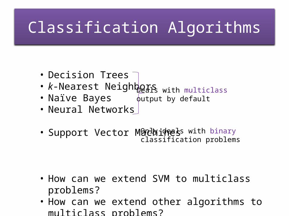
Classification Algorithms
• Decision Trees• k-Nearest Neighbors• Naïve Bayes• Neural Networks
• Support Vector Machines
• How can we extend SVM to multiclass problems?• How can we extend other algorithms to multiclass
problems?
Deals with multiclass output by default
Only deals with binary classification problems

One-against-one Approach
,
, ,
Dependent variable
training data where
Possible values: 1, 2, ,
For each pair , {1,2, , } where
•
binary classifier trained wi
or
•
Final classification is done by
th
voting
i j
i j i j
y
y k
i j k i j
y i yD
C D
j
*,
1, ,
(ties broken randomly)
( ) a ( ( )rg max )i jy k i j
I C x yC x

One-against-one Approach
,
, ,
Dependent variable
training data where
Possible values: 1, 2, ,
For each pair , {1,2, , } where
•
binary classifier trained wi
or
•
Final classification is done b
th
y voting
i j
i j i j
y
y k
i j k
y i yD
i j
C D
j
*,
1, ,
(ties broken randomly)
( ) a ( ( )rg max )i jy k i j
I C x yC x
Number of m
(
odels
2
1)
2
k k k

One-against-rest Approach
Possible values: 1, 2, ,
For each {1,2, , }
• Create training set as follows:
replace that value with
•
ot
Dep
her
endent variable
anytime
binary classifi
Final classi
er trained w
f
i
icati
th
i
i iC
y
y k
i k
D
y
D
y i
( ) one vote for
on is done by
( ) other one vote for each other val
voting (ties broken randomly)
• counts as
• counts as u e of i
i
C x i i
C x y