Math 3680

Lecture #19

Correlation and Regression

The Correlation Coefficient:

Limitations

0

5

10

15

20

25

30

-6 -4 -2 0 2 4 6

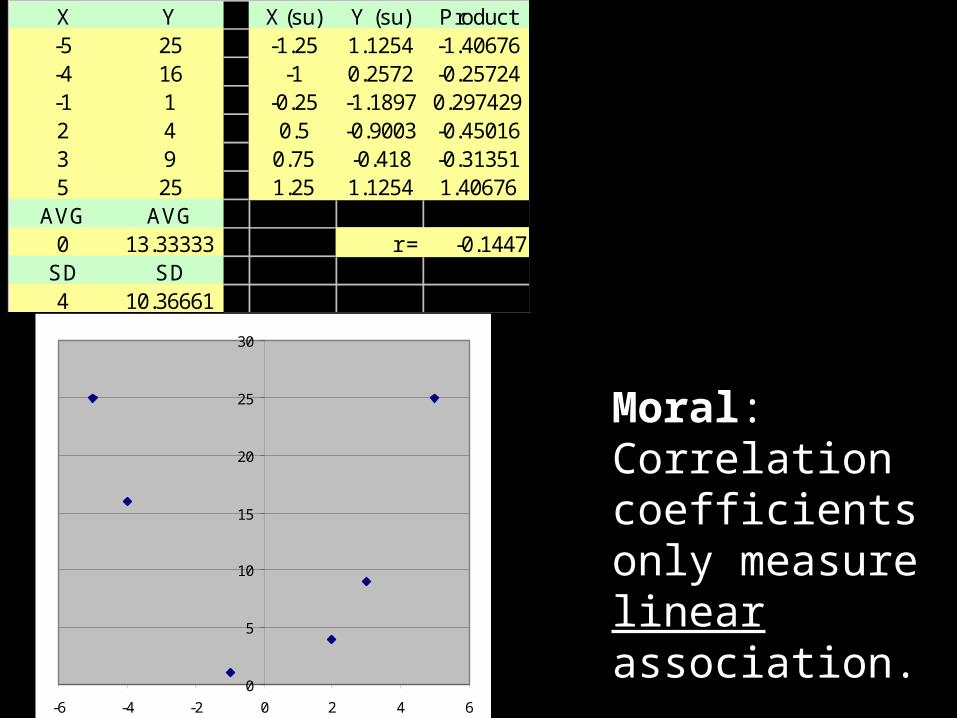
X Y X (su) Y (su) Product-5 25 -1.25 1.1254 -1.40676-4 16 -1 0.2572 -0.25724-1 1 -0.25 -1.1897 0.2974292 4 0.5 -0.9003 -0.450163 9 0.75 -0.418 -0.313515 25 1.25 1.1254 1.40676

AVG AVG0 13.33333 r = -0.1447

SD SD4 10.36661

Moral: Correlation coefficients only measure linear association.

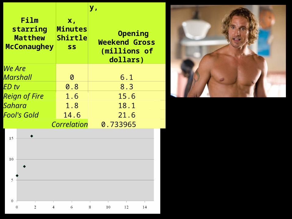
Film starring Matthew

McConaughey

x, Minutes Shirtless

y, Opening Weekend Gross (millions of dollars)

We Are Marshall 0 6.1ED tv 0.8 8.3Reign of Fire 1.6 15.6Sahara 1.8 18.1Fool's Gold 14.6 21.6

Correlation 0.733965

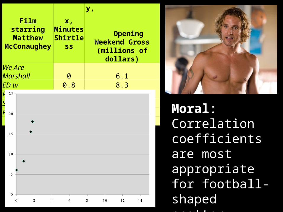
Film starring Matthew

McConaughey

x, Minutes Shirtless

y, Opening Weekend Gross (millions of dollars)

We Are Marshall 0 6.1ED tv 0.8 8.3Reign of Fire 1.6 15.6Sahara 1.8 18.1Fool's Gold

Correlation 0.966256

Moral: Correlation coefficients are most appropriate for football-shaped scatter diagrams and can be very sensitive to outliers.

Regression

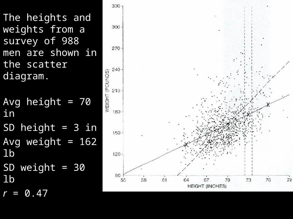
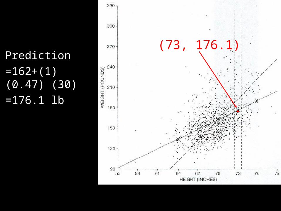
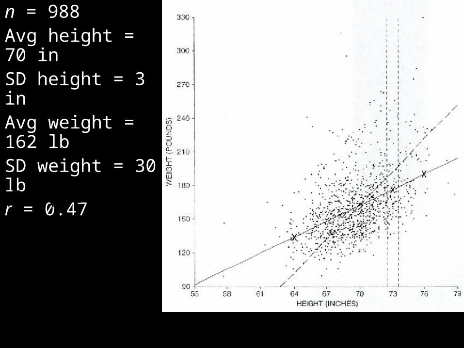
The heights and weights from a survey of 988 men are shown in the scatter diagram.

Avg height = 70 in

SD height = 3 in

Avg weight = 162 lb

SD weight = 30 lb

r = 0.47

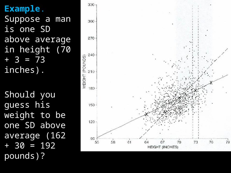
Example. Suppose a man is one SD above average in height (70 + 3 = 73 inches).

Should you guess his weight to be one SD above average (162 + 30 = 192 pounds)?

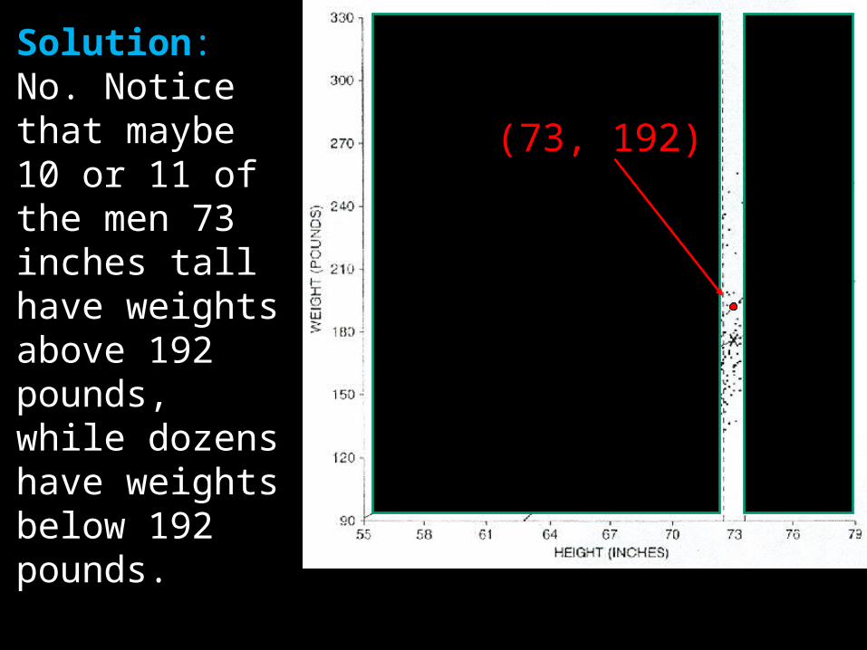
Solution: No. Notice that maybe 10 or 11 of the men 73 inches tall have weights above 192 pounds, while dozens have weights below 192 pounds.

(73, 192)

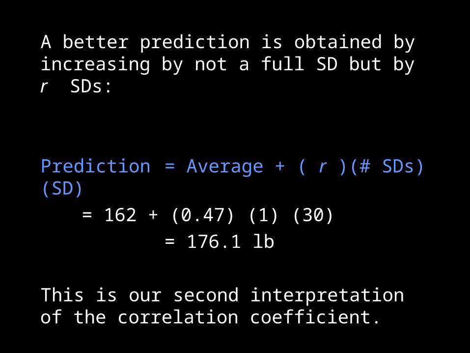
A better prediction is obtained by increasing by not a full SD but by r SDs:

Prediction = Average + ( r )(# SDs)(SD)

= 162 + (0.47) (1) (30)

= 176.1 lb

This is our second interpretation of the correlation coefficient.

Prediction

=162+(1) (0.47) (30)

=176.1 lb

(73, 176.1)

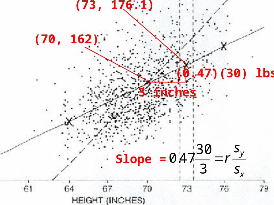
(73, 176.1)

(70, 162)

3 inches

(0.47)(30) lbs

Slope = x

y

s

sr

3

3047.0

Example: Predict the height of a man who is 176.1 pounds. Does this contradict our previous example?

Example: Predict the weight of a man who is 5’6”. Where does this prediction appear in the diagram?

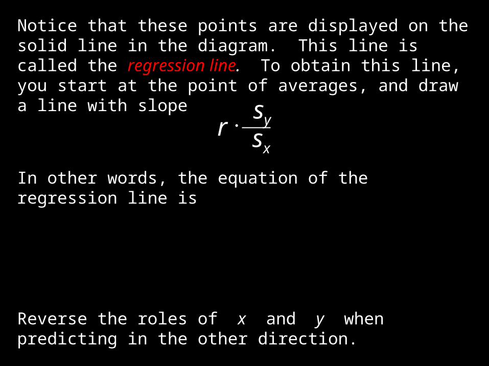
Notice that these points are displayed on the solid line in the diagram. This line is called the regression line. To obtain this line, you start at the point of averages, and draw a line with slope

In other words, the equation of the regression line is

Reverse the roles of x and y when predicting in the other direction.

sy r sx

)(ˆ xxs

sryy

x

y

Example: Find the equation of the regression line for the height-weight diagram.

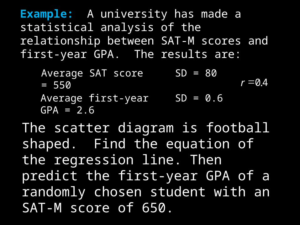
Average SAT score = 550 SD = 80

Average first-year GPA = 2.6 SD = 0.6

 

Example: A university has made a statistical analysis of the relationship between SAT-M scores and first-year GPA. The results are:

40.r

The scatter diagram is football shaped. Find the equation of the regression line. Then predict the first-year GPA of a randomly chosen student with an SAT-M score of 650.

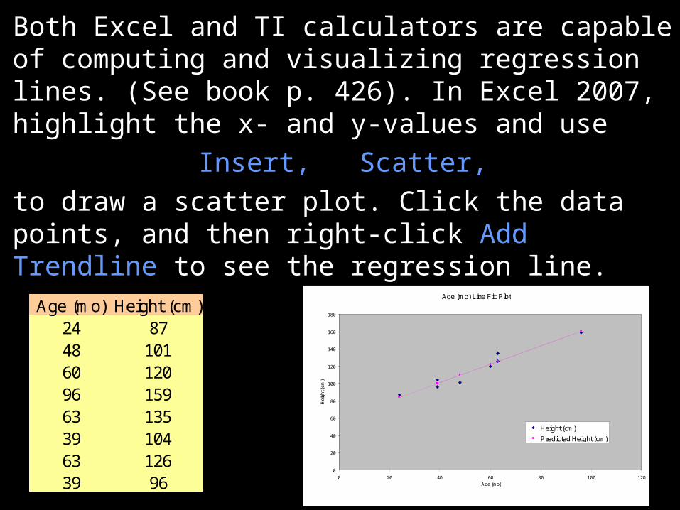
Both Excel and TI calculators are capable of computing and visualizing regression lines. (See book p. 426). In Excel 2007, highlight the x- and y-values and use

Insert, Scatter,

to draw a scatter plot. Click the data points, and then right-click Add Trendline to see the regression line.

Age (mo) Height (cm)24 8748 10160 12096 15963 13539 10463 12639 96

Age (mo) Line Fit Plot

0

20

40

60

80

100

120

140

160

180

0 20 40 60 80 100 120Age (mo)

Hei

ght (

cm)

Height (cm)

Predicted Height (cm)

The Regression Effect

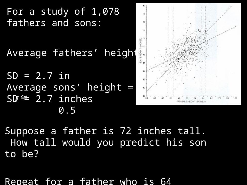
For a study of 1,078 fathers and sons:

Average fathers’ height = 68 inSD = 2.7 inAverage sons’ height = 69 inSD = 2.7 inches 0.5 r

Suppose a father is 72 inches tall. How tall would you predict his son to be?

Repeat for a father who is 64 inches tall.

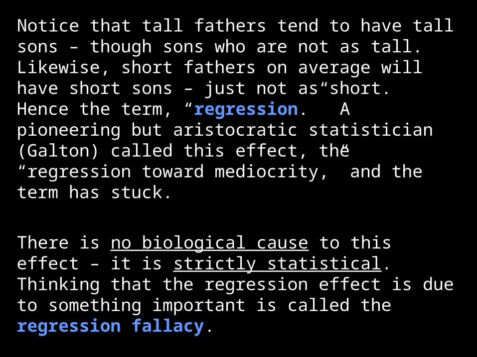
Notice that tall fathers tend to have tall sons – though sons who are not as tall. Likewise, short fathers on average will have short sons – just not as short. Hence the term, “regression.” A pioneering but aristocratic statistician (Galton) called this effect, the “regression toward mediocrity,” and the term has stuck.

There is no biological cause to this effect – it is strictly statistical. Thinking that the regression effect is due to something important is called the regression fallacy.

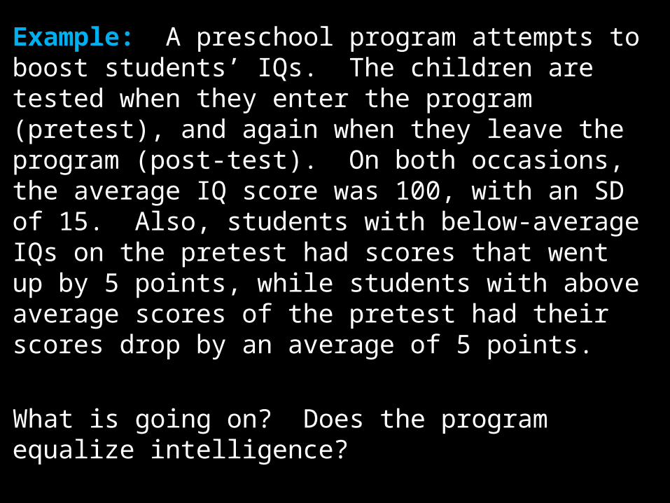
Example: A preschool program attempts to boost students’ IQs. The children are tested when they enter the program (pretest), and again when they leave the program (post-test). On both occasions, the average IQ score was 100, with an SD of 15. Also, students with below-average IQs on the pretest had scores that went up by 5 points, while students with above average scores of the pretest had their scores drop by an average of 5 points.

What is going on? Does the program equalize intelligence?

Example. Suppose someone gets a score of 140 on the pretest. Does this mean that the student has an IQ of exactly 140?

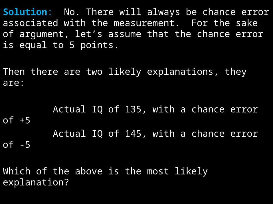
Solution: No. There will always be chance error associated with the measurement. For the sake of argument, let’s assume that the chance error is equal to 5 points.

Then there are two likely explanations, they are:

         Actual IQ of 135, with a chance error of +5

         Actual IQ of 145, with a chance error of -5

Which of the above is the most likely explanation?

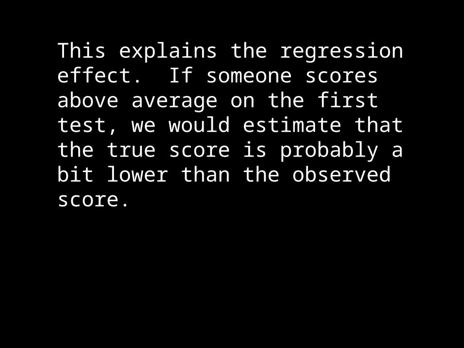
This explains the regression effect. If someone scores above average on the first test, we would estimate that the true score is probably a bit lower than the observed score.

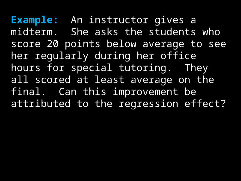
Example: An instructor gives a midterm. She asks the students who score 20 points below average to see her regularly during her office hours for special tutoring. They all scored at least average on the final. Can this improvement be attributed to the regression effect?

Regression and

Error Estimation

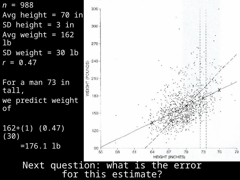
n = 988Avg height = 70 inSD height = 3 inAvg weight = 162 lbSD weight = 30 lbr = 0.47

For a man 73 in tall,we predict weight of

162+(1) (0.47) (30) =176.1 lb

Next question: what is the error for this estimate?Based on the picture, is it 30 lb? Or less?

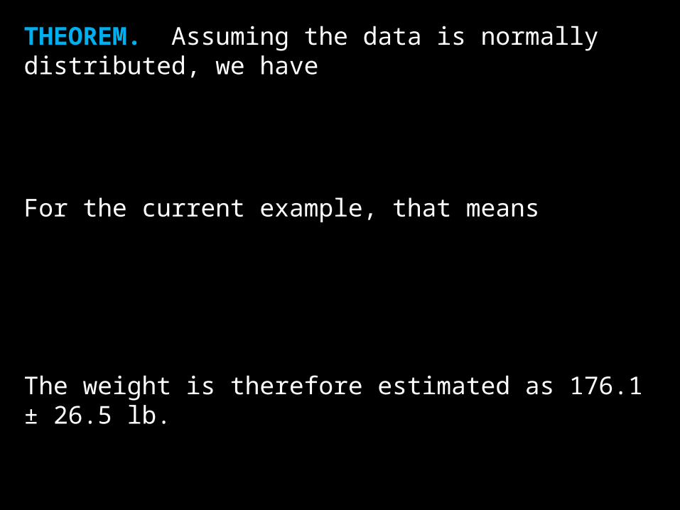
THEOREM. Assuming the data is normally distributed, we have

For the current example, that means

The weight is therefore estimated as 176.1 ± 26.5 lb.

2

11 2

n

nrss ye

5.26986

987)47.0(130 2 es

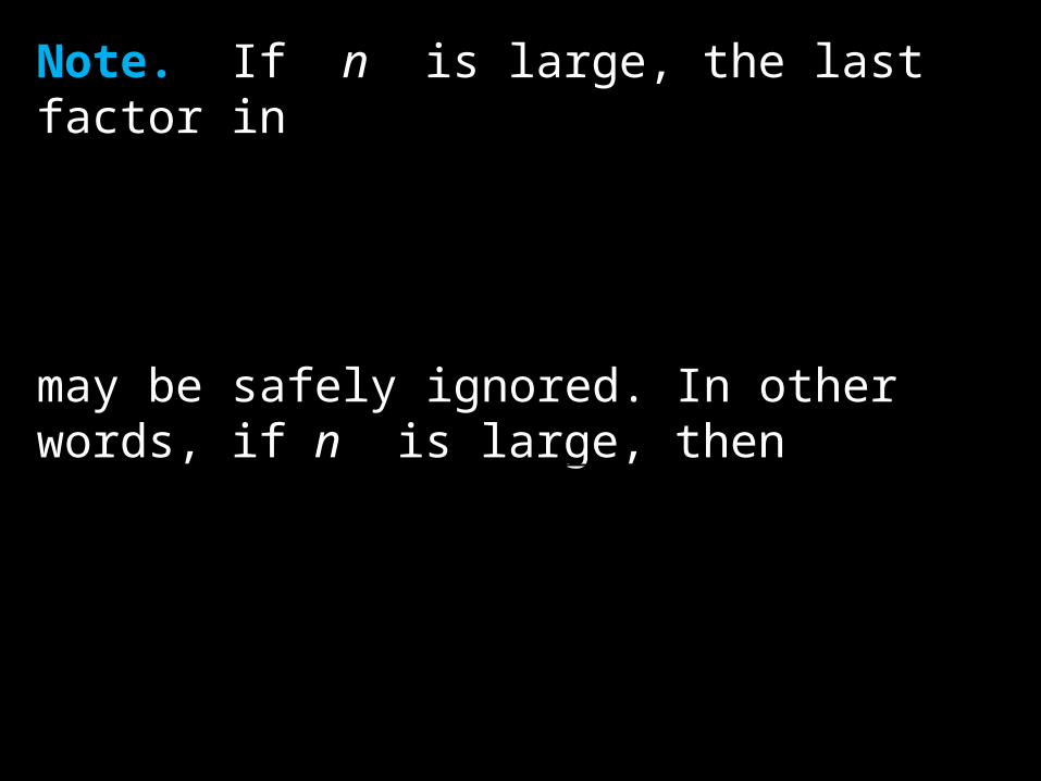
Note. If n is large, the last factor in

may be safely ignored. In other words, if n is large, then

2

11 2

n

nrss ye

21 rss ye

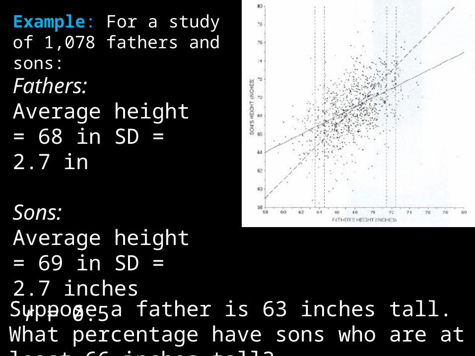
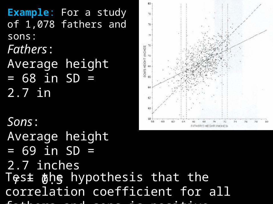
Example: For a study of 1,078 fathers and sons:

Fathers:Average height = 68 in SD = 2.7 in

Sons: Average height = 69 in SD = 2.7 inches r = 0.5

Suppose a father is 63 inches tall. What percentage have sons who are at least 66 inches tall?

Testing Correlation

Recall the equation of the regression line:

so that the slope of the regression line is .

The standard error for the slope is given by

)(ˆ xxs

sryy

x

y

x

y

s

srb

2

1

2

1

1

22

n

r

r

b

n

r

s

s

ns

sSE

x

y

x

eb

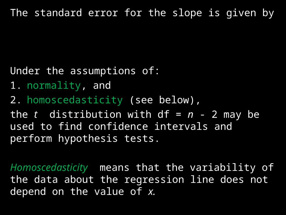
The standard error for the slope is given by

Under the assumptions of:

1. normality, and

2. homoscedasticity (see below),

the t distribution with df = n - 2 may be used to find confidence intervals and perform hypothesis tests.

Homoscedasticity means that the variability of the data about the regression line does not depend on the value of x.

2

1

2

1

1

22

n

r

r

b

n

r

s

s

ns

sSE

x

y

x

eb

n = 988Avg height = 70 inSD height = 3 inAvg weight = 162 lbSD weight = 30 lbr = 0.47

7.43

30)47.0(

b

281.0986

)47.0(1

47.0

7.4 2

bSE

For df = 986, the Student t distribution is almost normal. So a 95% confidence interval for the slope is

The corresponding confidence interval for the correlation coefficient for all men is

55.07.4)281.0)(96.1(7.4

055.047.0

Example: For a study of 1,078 fathers and sons:

Fathers:Average height = 68 in SD = 2.7 in

Sons: Average height = 69 in SD = 2.7 inches r = 0.5

Test the hypothesis that the correlation coefficient for all fathers and sons is positive.