Math 220 F11 Lecture Notes - Department of Mathematics · Math 220 F11 Lecture Notes William Chen...

Math 220 F11 Lecture Notes

William Chen

November 14, 2011

1. Lecture 1. Firstly, lets just get some notation out of the way.

Notation. R,Q,C,Z,N,∈,⊂,⊆, {}, ∅, A×B.

Everyone in high school should have studied equations of the form y = mx+ b. What does such anequation describe? It’s a line. Indeed, this is essentially where the “linear” in linear algebra comesfrom. Now, instead of thinking of this as the graph of the function

f(x) = mx+ b

we want to write it as x1 −mx2 = b and consider this as a linear equation in two variables.

Definition 1. (Linear equation). A linear equation in the variables x1, . . . , xn is an equation thatcan be written in the form

a1x1 + a2x2 + · · ·+ anxn = a0

where the coefficients ai ∈ R (ie, the ai’s are real numbers)

Examples. (Give examples and nonexamples of linear equations)

Once we view y = mx + b as the linear equation x1 − mx2 = b, we can talk about its solutionset. Whenever you have an equation in some variables, the solution set of the equation is just thecollection of assignments to the variables that make the equation true. In this case, we can also plotthe solution set on a graph with two axes, one for x1 and one for x2.

Example. Consider 2x1 + 3x2 = 0

Now, suppose we wanted to solve two such equations simultaneously. For example, suppose we had:

2x1 + 3x2 = 0

x1 − x2 = 1

How could we solve this? Now, if we plot the solution sets of these equations on a graph, what doesthe solution correspond to on the graph? Now consider an arbitrary system of linear equations in 2variables:

a1x1 + a2x2 = a

b1x1 + b2x2 = b

Some natural questions: Does it always have a solution, is the solution always unique? Examples?

Theorem 2. Any linear system has either 0, 1, or infinitely many solutions.

Definition 3. We say a system of linear equations (ie, a linear system) is consistent if it has atleast 1 solution, and inconsistent if it has no solutions.

Example. A good example of an inconsistent linear system is x = 1, x = 2.

A key object of study in this course is a matrix.

Definition 4. An m × n matrix is a rectangular array of numbers with m rows and n columns.Here, m× n is the size of the matrix.

1

Example. The following is a 2× 3 matrix[1 π 0−3 −2 1

3

]Now lets return to discussing systems of linear equations. The rest of the class will be spentdiscussing an algorithm for solving such systems. In fact, since systems can have 0, 1, or infinitelymany solutions, instead of “solving”, we are instead “determining the solution set” of the system.Consider this system:

x2 + 2x3 = 0

−x1 + 2x2 + x3 = 1

2x1 + 5x2 − x3 = −3

To solve this system, we need to make a few observations.

(a) (Interchange) If we interchange the positions of two equations, the resulting system has thesame solution set as the original.

(b) (Scaling) If we multiply any equation by a nonzero constant, the resulting system has the samesolution set.

(c) (Replacement) If we add a multiple of one equation to another equation, the resulting systemagain has the same solution set.

Proof. The first one is obvious. For (b), clearly it suffices to show that it doesn’t change the solutionset of the equation we’re scaling. To see this, suppose our original equation was:

a1x1 + a2x2 + a3x3 = a

then after multiplying by the nonzero constant c, we get

c(a1x1 + a2x2 + a3x3) = ca

We want to compare the solution sets of these two equations. Suppose (b1, b2, b3) is a solutionfor the first equation, then we see that a1b1 + a2b2 + a3b3 − a = 0, but that also means thatc(a1b1 + a2b2 + a3b3 − a) = 0, so (b1, b2, b3) is a solution to the second equation. Similarly, if(b1, b2, b3) is a solution to the second equation, then we know that c(a1b1 + a2b2 + a3b3 − a) = 0, sosince c 6= 0, we can multiply by 1/c to see that a1b1 + a2b2 + a3b3 − a = 0, so (b1, b2, b3) is also asolution to the first. Thus, we’ve shown that the two solution sets are the same, so scaling does notchange the solution set of the equation.

Lastly, for (c), since the operation only affects two equations, it suffices to show that the solutionset of the “subsystem” consisting of those two equations is unchanged by this operation. Let thoseequations be

a1x1 + a2x2 + a3x3 = a

b1x1 + b2x2 + b3x3 = b

and suppose we want to add c-times the first equation to the second, so the resulting system wouldbe:

a1x1 + a2x2 + a3x3 = a

c(a1x1 + a2x2 + a3x3) + b1x1 + b2x2 + b3x3 = b+ ca

Suppose (d1, d2, d3) is a solution to this system, then...etc

2

Now, with these observations, we can define an algorithm for computing solution set of any systemof linear equations. First, to simplify matters, we’ll represent the system in a more compact formusing matrices.

Definition 5. Suppose the system has n variables and m equations, then the coefficient matrix ofthe linear system is the m×n matrix whose (i, j)th entry is the coefficient of xj in the ith equation.

The augmented matrix of the system is coefficient matrix with an extra column added, where thejth entry of this column is the constant term in the jth linear equation.

Example. For the example given earlier, the coefficient and augmented matrices are 0 1 2−1 2 1

2 5 −1

0 1 2 0−1 2 1 1

2 5 −1 −3

The algorithm is difficult to describe, so we’ll just do it for a few examples

Examples.

x2 + 2x3 = 0

−x1 + 2x2 + x3 = 1

2x1 + 5x2 − x3 = −3

3

2. Lecture 2.

Quick review. Elementary row operations. Fundamental questions: existence and uniqueness.

Definition 6. A matrix is in echelon form if it has the following three properties:

(a) All nonzero rows are above any rows of all zeros.

(b) Each leading entry of a row is in a column to the right of the leading entry of the row above it.

(c) All entries in a column below a leading entry are zeros.

A matrix in echelon form is said to be in reduced echelon form if it satisfies the additional conditions

(d) The leading entry in each nonzero row is 1.

(e) Each leading 1 is the only nonzero entry in its column.

Definition 7. If a matrix A can be transformed into a matrix B via a sequence of elementary rowoperations, then we say that A is row-equivalent to B.

Note that any matrix that is row equivalent to the augmented matrix of some linear system describesa system with the same solution set.

Definition 8. A pivot position in a matrix A is a location/position in A that corresponds to aleading 1 in the reduced echelon form of A. A pivot column is a column of A that contains a pivotposition.

Note that pivots are not numbers. They are just locations in a matrix. The pivots of a matrix areproperties of its row-equivalence class, not of any particular matrix.

Algorithm for obtaining reduced row-echelon form. Let A be a matrix.

(a) Begin with leftmost nonzero column of A. This is a pivot column. This pivot position is at thetop.

(b) If the pivot position has a 0, interchange some rows to make it nonzero.

(c) Use row replacements to kill everything below the pivot position.

(d) Now let A be the matrix obtained by removing the first row and first column. Repeat steps1-3.

(e) Starting with the rightmost pivot and moving left, use row replacements to kill everythingabove each pivot.

4

3. Lecture 3.

Last time:

Definition 9. A matrix is in echelon form if it has the following three properties:

(a) All nonzero rows are above any rows of all zeros.

(b) Each leading entry of a row is in a column to the right of the leading entry of the row above it.

(c) All entries in a column below a leading entry are zeros.

A matrix in echelon form is said to be in reduced echelon form if it satisfies the additional conditions

(d) The leading entry in each nonzero row is 1.

(e) Each leading 1 is the only nonzero entry in its column.

Definition 10. If a matrix A can be transformed into a matrix B via a sequence of elementaryrow operations, then we say that A is row-equivalent to B. We’ll use the symbol ∼ to denoterow-equivalence. Ie, A ∼ B.t

Definition 11. A pivot position in a matrix A is a location/position in A that corresponds to aleading 1 in the reduced echelon form of A. A pivot column/row is a column/row of A that containsa pivot position.

Theorem 12. Each matrix is row-equivalent to exactly one reduced echelon matrix.

Definition 13. If A is the augmented matrix of some linear system, the basic variables of the systemare the variables that correspond to the pivot columns of A. The free variables of the system arethe variables that are not basic.

Definition 14. A linear system is consistent if it has at least one solution, and inconsistent other-wise.

Theorem 15. A linear system either has 0, 1, or infinitely many solutions.

– It is inconsistent if and only if the last column of its augmented matrix is a pivot column.

– It has a unique solution if and only if it is consistent and has no free variables.

– It has infinitely many solutions if and only if it is consistent and has at least one free variable.

Example. Solve the systems: 1 1 3 00 1 2 01 1 4 1

1 1 3 0

0 1 2 01 0 1 1

A general or parametric solution to a linear system identifies the free variables, and writes thebasic variables in terms of the free variables.

From the example, we can observe:

Theorem 16. Let A be a matrix, then the positions of the row leaders of A are the pivot positionsof A.

VECTOR SPACES

Idea of a vector, vector spaces over a field of coefficients/scalars F .

Definition 17. A vector space over F is a nonempty set V of objects called vectors, on which isdefined two operations, called addition and multiplication by scalars (elements of F ), such that thefollowing are true:

5

(a) For all u, v ∈ V , u+ v ∈ V .

(b) For all u, v ∈ V , u+ v = v + u.

(c) (u+ v) + w = u+ (v + w)

(d) There is zero vector 0 ∈ V , such that u+ 0 = u for all u ∈ V .

(e) For each u ∈ V , there is a vector v ∈ V such that u+ v = 0. We call this v “−u”.

(f) For every u ∈ V and c ∈ F , cu ∈ V .

(g) For all c ∈ F, u, v ∈ V , c(u+ v) = cu+ cv

(h) (c+ d)u = cu+ du

(i) c(du) = (cd)u

(j) 1u = u

We will mostly restrict our attention to vector spaces over R, ie, where F = R. If a vector space ismentioned without mention of its field of coefficients, we’ll assume that it’s R.

Example. Prove uniqueness of 0, uniqueness of inverses, 0u = 0, and (−1)u = −u.

Example. Last wednesday we discussed the set R2. These are the ordered pairs of real numbers(so (1, 2) 6= (2, 1)). We can represent each element in many ways, though often when we think of R2

as a vector space, we’ll want to write them as 2 × 1 matrices. Thus, elements of R2 will look like[ab

]. It’s important however to note that (a, b) is just as good a way to represent a vector in R2.

To make R2 into a vector space, we’ll define addition and multiplication as follows:[ab

]+

[cd

]=

[a+ cb+ d

]and for any c ∈ R, c

[ab

]=

[cacb

]Note that to talk about a set as a vector space, you need three pieces of information: its field ofcoefficients, and what addition and multiplication are on this set. For example, I can’t really ask ifthe set {0, 1} is a vector space, because I haven’t defined its field of coefficients, addition, or multi-plication. However, we can turn it into a vector space over itself if we define addition/multiplicationmod 2.

Verify this is a vector space. View these vectors as points in the plane. Can view vectors alsoas arrows. Talk about adding arrows.

Example. Let u = (3, 1). What does the set {cu : c ∈ R} look like? What about {cu+ v : c ∈ R}where v = (0, 1)? Lets relate these to linear equations. The first one contains all points that satisfyy = c, x = 3c. Substituting, we get x = 3y, or y = x/3. Repeat for other example.

Example. Introduce R3, then Rn.

Definition 18. For some vectors v1, . . . , vn in an vector space, a linear combination of v1, . . . , vn isan expression of the form:

c1v1 + c2v2 + · · ·+ cnvn ci ∈ R

Note that by properties (a) and (f), this is a vector, and property (c) allows us to omit parentheses.

Now let u, v ∈ R3. Given a vector w, is w a linear combination of u, v?

Theorem 19. Let v1, v2, . . . , vn, w be vectors, then the equation

x1v1 + · · ·+ xnvn = w

has the same solution set as the linear system whose augmented matrix is[v1 v2 · · · vn w

]Definition 20. Let v1, . . . , vn ∈ V , then the set of all linear combinations of v1, . . . , vn is denotedby Span {v1, . . . , vn} and is called the subset of V spanned/generated by v1, . . . , vn.

6

Thus, asking if a vector w is a linear combination of u, v is the same as asking if w ∈ Span {u, v}.Exercise. Let A be a set of vectors in V , then must 0 ∈ Span A?

Prove the following:

1. Span {(1, 0, 0), (0, 1, 0), (0, 0, 1)} = R3.

2. Span {(1, 0, 0), (0, 1, 0), (2,−5, 0)} 6= R3.

7

4 Lecture 4

ANNOUNCEMENTS: Theory Quiz next tuesday, definitions list online.

QUICK REVIEW OF LAST TIME.

Consider R3. Let u, v ∈ R3. What does Span {u} look like? What about Span {u, v}? Can you find2 vectors that span R3? What about 3 vectors?

Example. At the store, there are two sets of legos. Set A comes with 4 green blocks, 4 blue blocks,and 2 red block. Set B has 3 green, 4 blue, and 5 red. To build a spaceship, you need exactly 19green blocks, 22 blue blocks, and 20 red blocks. Is it possible to buy some number of sets A and Bto have exactly enough to build your spaceship?

Definition 21. A subspace of a vector space V is a subset W ⊆ V such that for any x, y ∈ W ,x+ y ∈W , and for any x ∈W, c ∈ R, cx ∈W .

Theorem 22. A subspace of a vector space is itself a vector space.

Exercises.

(a) Let v1, . . . , vn ∈ V . Is Span {v1, . . . , vn} a subspace?

(b) Is 0 ∈ Span {v1, . . . , vn}?(c) Come up with two vectors v, w ∈ R2 such that Span {v, w} is a line.

(d) Come up with three vectors u, v, w ∈ R3 such that Span {u, v, w} is a line.

(e) Let u = (1, 1), and v = (2, 3). What is Span {u, v}? Write (0, 0) as a linear combination ofu, v. Write (a, b) as a linear combination of u, v.

(f) Let u = (1, 2, 3), v = (6,−1, 0), and w = (−1,−1, 2). What is Span {u, v, w}?(g) Suppose a lego spaceship requires 5 red blocks, 3 green blocks, and 3 black blocks, and a lego

car requires 2 red blocks, 4 green blocks, and 2 black blocks. Lastly, a lego death star requires 1red block, 2 green blocks, and 8 black blocks. Suppose you have 31 red blocks, 20 green blocks,and 40 black blocks. Is it possible to build a collection of spaceships/cars/death stars and haveno blocks left over? If so, how many of each can you build?

Definition 23. If A is an m × n matrix with columns a1, . . . , an, and x = (x1, . . . , xn) a columnvector in Rn, we define the product Ax to be the (column) vector x1a1 + · · ·+ xnan.

This only makes sense if the number of columns of A equals the number of entries of x.

8

Lecture 5. Homework due today, definitions quiz next tuesday.

Is Span {(1, 1, 2), (5, 1, 10), (−1,−1, 3)} = R3?

Why can’t 1 vector span R2? (change one of the vectors coordinates, that wont be in the span!) Whycan’t 2 vectors span R3? Sure, it makes sense in these two cases, but why can’t say, 10 vectors spanall of R11? You can see the pattern and while you might be able to generalize to higher dimensions,to really be able to understand it you need to formulate a rigorous argument.

LAST TIME:

Ask for definitions of span and linear combination.

Definition 24. If A is an m × n matrix with columns a1, . . . , an, and x = (x1, . . . , xn) a columnvector in Rn, we define the product Ax to be the (column) vector x1a1 + · · ·+ xnan.

This product allows us to write our equations in terms of matrices. Let A be an m× n matrix withcolumns a1, . . . , an, and x, b ∈ Rn. Compare the two equations:

Ax = b x1a1 + · · ·+ xnan = b

By the definition of matrix multiplication, they’re exactly the same equation. Thus, we see that

Theorem 25. For a matrix A, the equation Ax = b has a solution if and only if b is a linearcombination of the columns of A

Recall:

Theorem 26. An augmented matrix A represents an inconsistent linear system iff the last columnis a pivot column.

Theorem 27. Let A be an m× n matrix. Then the following are equivalent:

(a) For each b ∈ Rm, Ax = b has a solution.

(b) For each b ∈ Rm, the augmented matrix [A b] represents a consistent system.

(c) Each b ∈ Rm is a linear combination of the columns of A.

(d) The columns of A span Rm.

(e) A has a pivot position in every row.

Proof. Clearly the first 4 are the same. For (c) =⇒ (d), suppose the REF of A does not have a pivotposition in every row, then the row without a pivot must be a zero row and must be on the bottom.Let v = (0, . . . , 0, 1). Now suppose B is the REF of A, then consider the (augmented) matrix [B v].Clearly [B v] is inconsistent. Reverse the row reduction process to obtain an augmented matrix[A w]. Since [B v] is inconsistent, so is [A w], and hence Ax = w does not have a solution, so thecolumns of A could not have spanned Rm. Thus, if they do span Rm, A must have a pivot in everyrow!

Example: Consider the matrix

A =

0 −6 −41 3 52 0 6

Find a vector b such that Ax = b is inconsistent.

For (d) =⇒ (c), suppose A has a pivot in every row, then consider the matrix [A (x1, . . . , xm)].Applying the same operations to this matrix as the ones used to row-reduce A will also give an REFmatrix that looks like [B (y1, . . . , ym)] where since B has a pivot in every row, the last column of[B (y1, . . . , ym)] is not a pivot, so the system is consistent, so the original system was consistent, nomatter what the xi’s are!

9

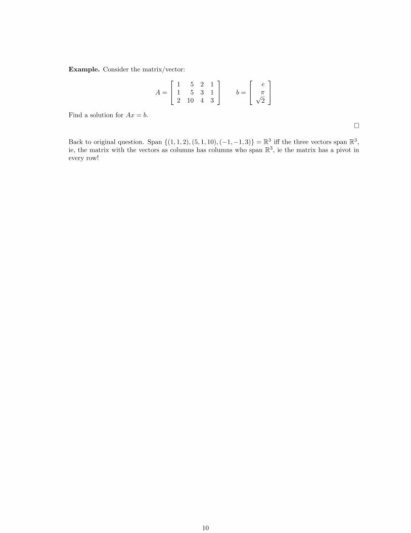
Example. Consider the matrix/vector:

A =

1 5 2 11 5 3 12 10 4 3

b =

eπ√2

Find a solution for Ax = b.

Back to original question. Span {(1, 1, 2), (5, 1, 10), (−1,−1, 3)} = R3 iff the three vectors span R3,ie, the matrix with the vectors as columns has columns who span R3, ie the matrix has a pivot inevery row!

10

6. Lecture 6. QUIZ TODAY. Problem set 3 is online. Thursday office hours moved to 1pm - 2:15pm.

Theorem 28. If A is an m× n matrix, and u, v ∈ Rn, and c ∈ R, then

(a) A(u+ v) = Au+Av

(b) A(cu) = c(Au)

Proof. Do examples with

A =

[1 5 20 −2 1

]u =

102

v =

31−1

(don’t compute any sums)

Definition 29. A system of linear equations is homogeneous if it can be written in the form Ax = 0.(ie, if all the constant terms are 0).

Give examples. Ask for example of homogeneous system that has no solutions. In fact, allhomogeneous systems have at least one solution. (Which solution?) Together with the existenceand uniqueness theorem of 1.2, we have:

Theorem 30. A homogeneous equation Ax = 0 has a nontrivial solution if and only if the equationhas at least one free variable (when viewed as a linear system).

Exercise. Is the following systems homogeneous? Does it have any nontrivial solutions? (findgeneral solutions) 3 1 11 0

3 2 13 01 1 5 0

What about 3x1− 6x2 + 12x3 = 0? (write as augmented matrix, row reduce, find general solutions)

What do these general solutions look like? Write general solutions in parametric form.

Theorem 31. Let A be an m × n matrix. The solution set to the equation Ax = 0 can be writtenas Span {v1, . . . , vk}. In particular, the solution set is a subspace of Rn.

The fact that it’s a subspace also follows from the linearity of matrix multiplication A(u + v) =Au+Av,A(cu) = c(Au).

Now let b 6= 0, so that Ax = b is nonhomogeneous. Suppose p is a solution to Ax = b, and q is asolution to Ax = 0. Must p+ q be a solution to Ax = b? In fact, all solutions are of this form:

Theorem 32. Let p be a solution to the equation Ax = b, and let W be the solution set of Ax = 0.Then the solution set of Ax = b is the set:

p+W = {p+ w : w ∈W}

Exercise. Write the general solution of Ax = b in parametric vector form.

A =

1 2 02 4 10 0 0

b =

100

In general, to write the solution set of a consistent system in parametric vector form:

(a) Reduce the augmented matrix to reduced echelon form.

(b) Express each basic variable in terms of free variables and/or constants.

(c) Write a typical solution x as a vector whose entries depend on the free variables.

(d) Decompose x into a linear combination of vectors using free variables as parameters.

Introduce as much of linear independence as possible.

11

7. Lecture 7

Linear Independence! Look at example 3 in section 1.5 for a good example of finding parametricforms.

Review: go over homogeneous systems...geometric view of solutions sets as being shifted subspaces.

LAST TIME:

Theorem 33. Let A be a matrix, b a vector. Let W be the solution set of Ax = 0, and let p be afixed solution of Ax = b, then the solution set of Ax = b is exactly p+W .

Question: Suppose Ax = 0 has a nontrivial solution. How many solutions does Ax = b have? CanAx = b has a different number of solutions than Ax = 0? Note that the above theorem says nothingabout the case when Ax = b is inconsistent! In general,...

Theorem 34. If Ax = b is consistent, then it has exactly the same “number” of solutions (ie, either1 or ∞) as Ax = 0.

Purpose: Consider two vectors in R2. What are the possibilities for their span? When is it a point,a line, a plane? What about 3 vectors in R3? Today, we’ll try to pinpoint exactly what propertythose three vectors must have.

Definition 35. A (finite) set of vectors S = {v1, . . . , vp} ∈ Rn is said to be linearly independent ifthe vector equation:

x1v1 + · · ·+ xpvp = 0

has only the trivial soution. They are said to be linearly dependent if they are not linearly indepen-dent (ie, there exists a nontrivial solution).

Or, equivalently, S is linearly independent if the matrix equation [v1 v2 . . . vp]x = 0 has only thetrivial solution.

Example. Columns of the matrices 1 3 8 10 −1 3 23 1 1 0

1 3 10 −1 11 2 3

Special Cases. Let S ⊂ Rn contain only one vector. When is S linearly dependent? What if|S| = 2?

Theorem 36. A set S ⊂ Rn consisting of one vector is linearly dependent if and only if S = {0}.If |S| = 2 (say S = {u, v}, u 6= v), then S is linearly dependent if and only if one of the vectors is amultiple of the other.

Theorem 37. A set S ⊆ Rn of two or more vectors is linearly dependent if and only if at least oneof the vectors in S is a linear combination of the others.

Proof. Let S = {v1, . . . , vp} be such a set of vectors, then to say that S is linearly dependent is tosay that there exist a nontrivial solution x1, . . . , xn to the equation

x1v1 + · · ·+ xpvp = 0

rearranging, we get:

x1v1 = −x2v2 − x3v3 − · · · − xpvp → v1 = −x2x1v2 − · · · −

xpx1vp

Where did we use the fact that the solution is nontrivial? Can we always say that every v ∈ S canbe written as a linear combination of the others?

Theorem 38. Let S ⊆ Rn, then if |S| > n, S is linearly dependent.

12

8. Lecture 8.

Consider the equation Ax = b. Solving the equation amounts to finding a vector such that whenmultiplied by A, gives you b. Thus, we see that “multiplication by A” is a way of transformingvectors into other vectors. The right terminology for this is a function.

For another simple example, consider the function f(x) = x2.

Definition 39. Let A,B be sets, then a function/map/transformation f from A to B is denotedf : A → B and is a rule that assigns an element of B to every element of A. In a way, we thinkof f as being a machine that when fed an element of A, spits out an element of B. Here, A is thedomain, and B is the codomain. If a ∈ A, then we say that T (a) is the image of a (under T ), andwe say that the range of T is the set of all images T (a) for a ∈ A.

Examples. f : R → R defined by f(x) = x, f(x) = x2. Also, f : R2 → R3 given by f(x, y) =(x, y, 0). (What are the images of these?)

Definition 40. Let V,W be vector spaces (for example, V = Rn, W = Rm), then function T : V →W is called a linear transformation if:

(a) For all u, v ∈ V , T (u+ v) = T (u) + T (v)

(b) For all u ∈ V, c ∈ R, T (cu) = cT (u)

Theorem 41. If T : V → W is a linear transformation, then for any v1, . . . , vn ∈ V , anda1, . . . , an ∈ R, we have

T (a1v1 + · · ·+ anvn) = a1T (v1) + · · ·+ anT (vn)

Example. Let T : R2 → R2 be given by T ((x, y)) = (x + y, 2x − y). Is this linear? Let u = (1, 0)and v = (1, 1). What is T (u), T (v)? What is T ((12,−3))?

So far we’ve thought of Ax = b as a linear system. But now, we see it in a new light:

Let A be an m× n matrix, then we define the map: TA : Rn → Rm by TA(x) = Ax. Is TA a lineartransformation?

Here, we essentially view A as a function that maps vectors in Rn to vectors in Rm via multiplication.

Notation. From now on, we write ei to be the vector with 1 in the ith coordinate, and 0’s everywhereelse. The set {e1, . . . , en} are called the canonical basis vectors of Rn.

Examples. Let

A =

[1 −2 3−1 0 1

]B =

1 23 −10 1

b =

[22

]u =

12−1

Find TA(u). Is b in the range of TA? Is u in the range of TB? How many vectors does TA map tob? How many vectors does TB map to u? Recall the theorems:



(e) A has a pivot position in every row.

Theorem 43. Let S ⊆ Rn, then if |S| > n, S is linearly dependent.

Example. Consider various matrices.[0 −11 0

], [ 1 0

0 1 ] , [ 2 00 2 ]. Compute TA(ei). Note that they’re just

the columns of the matrices.

13

9. Lecture 9 Section 1.9 in the book.

New homework online, DUE THURSDAY

LAST TIME:

Definition 44. Let V,W be vector spaces, then a function T : V → W is called a linear transfor-mation if:

(a) For all u, v ∈ V , T (u+ v) = T (u) + T (v)

(b) For all u ∈ V, c ∈ R, T (cu) = cT (u)

In particular, this means that T (0) = T (0 ·u) = 0 ·T (u) = 0, ie any linear transformation maps 0 to0 (so if T is a function with T (0) 6= 0, then T is not linear)

Theorem 45. Let v1, . . . , vn ∈ V (a vector space), a1, . . . , an ∈ R, and T : V → W a lineartransformation. Then

T (a1v1 + · · ·+ anvn) = a1T (v1) + · · ·+ anT (vn)

Corollary 46. Suppose v1, . . . , vp ∈ Rn span Rn, then any linear transformation T : Rn → Rm iscompletely determined by how it acts on v1, . . . , vn.

In particular, if v1, . . . , vp span Rn and you know the values T (v1), . . . , T (vp), then you can calculateT (v) for ANY v ∈ Rn.

Notation. From now on, we’ll refer to ei as being the vector with a 1 in the i-th position and zeroeseverywhere else. Note that this vector will depend on context. For example,

e2 ∈ R2 is

[01

]but e2 ∈ R3 is

010

Corollary 47. Any linear transformation T : Rn → Rm is completely determined by its action onthe canonical basis vectors e1, . . . , en ∈ Rn.

Example. Suppose T : R3 → R2 is a linear transformation, and

v1 =

011

v2 =

222

v3 =

−103

T (v1) =

[30

], T (v2) =

[06

], T (v3) =

[−312

]

What is T (e1), T (e2), T (e3)? Since the domain of T is R3, e1 =

100

, e2 =

010

, e3 =

001

Hint: For each i = 1, 2, 3, solving for [v1 v2 v3]x = ei will show e1 = −v1+ 1

2v2, e2 = 43v1−

16v2−

13v3,

and e3 = − 13v1 + 1

6v2 + 13v3.

Now consider A =

[−3 5 −2

3 −5 4

]. Let e1 =

100

, e2 =

010

, and e3 =

001

.

What is TA(e1), TA(e2), TA(e3)? What is Span {e1, e2, e3}? (Answer: TA(ei) = T (ei)!) But thecorollary tells us that any linear transformation is completely determined by how it acts on e1, e2, e3(or any other spanning set!) Thus, T must be the same transformation as TA! Indeed, for any x, y, z,we have

T

xyz

= T (xe1 + ye2 + ze3) = xT (e1) + yT (e2) + zT (e3)

14

but also

TA

xyz

= TA (xe1 + ye2 + ze3) = xTA(e1) + yTA(e2) + zTA(e3)

But since TA(ei) = T (ei), we have T (x, y, z) = TA(x, y, z)! Thus, this means that any lineartransformation can be represented by a matrix!

Theorem 48. Let T : Rn → Rm be a linear transformation, then there is a unique matrix AT suchthat T (x) = Ax for all x ∈ Rn. In fact, AT = [T (e1) T (e2) . . . T (en)]. We call this matrix AT the(standard) matrix for T .

Proof. Any linear transformation from Rn → Rm is completely determined by their action one1, . . . , en. Thus, if two linear transformations behave the same way on e1, . . . , en, then they mustbe the same transformation.

To see why it’s unique, note that if A is a matrix that represents the transformation T , then for allx ∈ Rn, TA(x) = T (x). In particular, for each i, TA(ei) = T (ei), but TA(ei) is also the ith columnof A, so A must be the matrix with columns T (ei).

Examples. Let T : R2 → R2 be the linear transformation defined by rotating everything counter-clockwise by 90◦, and the reflecting across the x-axis. Find AT (the standard matrix for T )

Definition 49. A function f : A→ B is said to be onto if the range of f is equal to the codomain.

Definition 50. A function f : A→ B is said to be one-to-one (as opposed to many-to-one) if eachb ∈ B is the image of at most one a ∈ A.

Example. Are the following functions 1-1? (ie, one-to-one), are they onto?

(a) f : R→ R, where f(x) = 3x

(b) f : R→ R, where f(x) = ex (1-1 but not onto)

(c) f : R→ R, where f(x) = x3 − x (onto but not 1-1, since it has three roots)

(d) f : R→ R, where f(x) = x2 (neither 1-1 nor onto)

Note that with these definitions, we can extend an earlier theorem as follows:



(b) For each b ∈ Rm, the augmented matrix [A b] represents a consistent system.

(c) Each b ∈ Rm is a linear combination of the columns of A.


(e) A has a pivot position in every row. (ie, all rows are pivot rows)

*(f) TA : Rn → Rm is onto.

In fact, we have the following fact:

Theorem 52. If T : Rn → Rm is a linear transformation, then the range of T is the span of thecolumns of AT .

Proof. The range of T is by definition the set of all things that look like T (~x) for some ~x =(x1, . . . , xn) ∈ Rn. But by definition of AT , if ~a1, . . . ,~an are the columns of AT , we have

T (~x) = ATx = x1~a1 + · · ·+ xn~an

where the second equality is just the definintion of multiplying a matrix by a vector. Thus, we seethat T (~x) is a linear combination of the columns of AT . From this, noting that x1, . . . , xn are freeto range over all possible real numbers, we see that the set of all T (~x) = AT~x is exactly the set ofall linear combinations of ~a1, . . . ,~an.

Corollary 53. Let T : Rn → Rm be a linear transformation, then T is onto if and only if thecolumns of AT span Rm.

15

10. Lecture 10 Sections 1.9 and 2.1 in the book.

Recall that theorem 51 gave us some characterizations of what it means for a linear transformationto be onto. Today, we discuss what it means for a linear transformation to be 1-1, and then continueon to discuss how to do algebra with matrices.

Theorem 54. Let T : Rn → Rm be a linear transformation, then the following are equivalent:

(a) T is one-to-one.

(b) T (x) = 0 has only the trivial solution.

(c) The columns of AT are linearly independent.

(d) There is a pivot in every column of AT . (ie, all columns are pivot columns)

Proof. First we show (a)⇐⇒ (b) If T is 1-1, then in particular T can map at most one thing to 0,and since T (0) = 0, this means that T (x) = 0 must have only the trivial solution. Conversely, if Tis not one-to-one, then suppose for distinct vectors u 6= v ∈ V , we have T (u) = T (v), then

T (u)− T (v) = 0 = T (u− v)

but that since u 6= v, u− v 6= 0, so u− v is a nontrivial solution to T (x) = 0. This shows that (a) isexactly the same as (b).

To see that (b)⇐⇒ (c), note that by the definition of AT , T (x) = ATx. Thus, the equation T (x) = 0is the same as the equation ATx = 0, and the latter equation only having a trivial solution is exactlyto say that the columns of AT are linearly independent.

Lastly to show that (d) is the same as (a),(b),(c), note that: [T (x) = ATx = 0 has a unique solution]⇐⇒ [there are no free variables] ⇐⇒ [all variables are basic] ⇐⇒ [every column correspondingto a variable in the augmented matrix [AT

~0] contains a pivot]

Thus (d) is the same as (b), which are the same as (a) and (c), so all of the statements (a),(b),(c),(d)are the same.

Example. What is the domain/codomain/range of TA? Is TA onto? 1-1?

A =

1 3 −20 5 10 0 80 0 0

Domain is R3, codomain is R4. The range of TA is the span of the columns. Since not every rowcontains a pivot, by 51, TA is not onto. Since every column is a pivot column, by 54, TA is 1-1.

MATRIX OPERATIONS

Let A be a matrix, then we’ll use aij to denote the number in the ith row and jth column.

Definition 55. Let A,B be matrices of the same size (say m × n). Then we define the matrixA+B to be the matrix C such that cij = aij + bij for all 1 ≤ i ≤ m and 1 ≤ j ≤ n.

For any r ∈ R, we define the scalar multiple rA to be the matrix D such that dij = raij .

The zero matrix is a matrix with all zero entries, which we’ll often denote with 0.

In other words, we add matrices by adding corresponding entries, and multiply matrices by scalarsby scaling corresponding entries.

Example. Ie,[1 23 4

]+

[0 16 1

]=

[1 39 5

], and 2

[1 23 4

]=

[2 46 8

]Addition and scalar multiplication of matrices satisfy the usual rules:

16

Theorem 56. Let A,B,C be matrices of the same size, and let r, s ∈ R.

(a) A+B = B +A

(b) (A+B) + C = A+ (B + C)

(c) A+ 0 = A

(d) r(A+B) = rA+ rB

(e) (r + s)A = rA+ sA

(f) r(sA) = (rs)A

Proof. These all follow directly from the definitions. Do some examples until you believe theseproperties.

Definition 57. Let A be an m× n matrix, and let B be an n× p matrix with columns ~b1, . . . ,~bp.Then define the product of A and B as:

AB = [A~b1 A~b2 · · · A~bp]

In light of this definition, note that multiplying a matrix by a vector is a special case of multiplyingtwo matrices. (ie, the vector is just an m× 1 matrix.)

Exercise 58. If A is m× n, and B is n× p, what is the size of AB?

Example 59. Verify these:[1 00 1

] [1 23 4

]=

[1 23 4

]and

[1 2 00 −1 1

] 3 1 0−1 2 0

0 −2 0

=

[1 5 01 −4 0

]

On the other hand, 3 1 0−1 2 0

0 −2 0

[ 1 2 00 −1 1

]is undefined!!!

The Row-Column rule for matrix multiplication. Suppose A,B are matrices of appropriatesizes, where say B = [~b1 · · · ~bp], then the ij-th entry of AB is the ith entry of A~bj . To compute

that, by the row-column rule for vectors, the ith entry of A~bj is just ~ai ·~bj , where · denotes the dotproduct, and ~ai is the ith row of A.

Definition 60. Let Im be the m×m matrix with 1’s along the main diagonal and 0’s everywhereelse. We’ll call Im the m ×m identity matrix. If the size is clear from context, we sometimes justuse the letter I.

Example 61. I2 =

[1 00 1

], and I3 =

1 0 00 1 00 0 1

.

Theorem 62. Let r ∈ R, A be an m× n matrix, and let B,C have sizes for which the expressionsbelow make sense.

(a) A(BC) = (AB)C

(b) A(B + C) = AB +AC

(c) (B + C)A = BA+ CA

(d) r(AB) = (rA)B = A(rB)

(e) ImA = A = AIn

Proof. These all follow directly from the definitions. Do some examples until you believe theseproperties.

17

Of these, (a) is especially interesting. While at first it may seem like a technicality, to understandwhat it means, consider the following example.

Example 63. Suppose A is 4×3, and B is 3×2. Then, we have the associated linear transformationsTA : R3 → R4 and TB : R2 → R3. (What are the standard matrices of TA, TB?)

Now, consider the map T : R2 → R4 defined by first sending any vector x ∈ R2 to TB(x), and thensending TB(x) to TA(TB(x)). Pictorially, we have the following diagram:

T : R2 TB // R3 TA // R4

x� // TB(x)

� // TA(TB(x))

x � // Bx � // A(Bx)

Ie, T is the composition of the linear transformations TA and TB , denoted T = TA ◦ TB , whereT (x) = TA(TB(x)). In other words, T is the map obtained by first applying TB , and then TA.

Referring to the above diagram, T is defined by the rule: “for any x ∈ R2, T (x) = A(Bx)”.

Now, using 62(a) and setting C = x, we find A(Bx) = (AB)x. Thus,

T (x) = A(Bx) = (AB)x

What’s the standard matrix for T?

Since T (x) = (AB)x, by the definition of the standard matrix, the standard matrix for T is AB!(ie, T = TAB)

In particular, since T is the map defined by “multiplication by AB”, T is a linear transformation.We summarize this in the following theorem.

Theorem 64. Let TB : Rp → Rn, and TA : Rn → Rm be linear transformations given by theirstandard matrices A,B. Then the composition TA ◦ TB is a linear transformation from Rp → Rm

defined by“starting in Rp, apply TB, then apply TA and land in Rm”

More precisely, (TA ◦ TB)(x) = TA(TB(x)). Furthermore, the standard matrix for TA ◦ TB is AB.

Also, AS is m× n, AT is n× p, so ASAT is m× p.

Example 65. Suppose A =

[0 11 0

]. Note that[

0 11 0

] [a bc d

]=

[c da b

]Suppose T : R2 → R2 is the map defined by first rotating counterclockwise by 90◦, and then reflectingacross the line x = y. What is the standard matrix for T?

The usual method involves computing T (e1) and T (e2). Then, the standard matrix is just [T (e1) T (e2)],

which in this case is

[1 00 −1

].

Here’s another (not necessarily easier) way to think about it. Firstly,

– let R : R2 → R2 be the linear transformation “Rotate counterclockwise by 90◦”

– let F : R2 → R2 the linear transformation “reFlect across the line x = y”.

Note that the standard matrix for R is the matrix AR =

[0 −11 0

], and the standard matrix for

F is AF = A (the matrix above).

Then, the entire transformation T is really just the composition F ◦R (ie, first Rotate, then reFlect).theorem 64 tells us that T is indeed a linear transformation, and its standard matrix is AFAR, ie

By theorem 64 the standard matrix of T is

[0 11 0

] [0 −11 0

]=

[1 00 −1

]

18

WARNING 66.

(a) In general, AB 6= BA.

In the above example, note that AFAR =

[1 00 −1

], but ARAF =

[−1 0

0 1

]. Indeed,

AFAR represents the transformation “first rotate, then reflect”, and ARAF represents thetransformation “first reflect, then rotate”. Think about what these transformations do to e1(or e2)

(b) Cancellation laws do not in general hold for matrix multiplication. That is, even if AB = AC,that does not mean that B = C. (See exercise 2.1.10 in the book)

(c) If AB = 0 (ie, the zero matrix), then from this information alone you cannot conclude thateither A = 0 or B = 0. (See exercise 2.1.12 in the book)

MATRIX TRANSPOSE

We probably won’t have time to get to this, but matrix transposes are pretty easy. They’re just a“flipped” version of the matrix. Here’s the precise definition and some properties.

Definition 67. Let A be m×n, then the transpose of A is denoted AT and has entries (aT )ij = aji.

Theorem 68. Let A,B denote matrices of appropriate sizes, then

(a) (AT )T = A

(b) (A+B)T = AT +BT

(c) For any scalar r, (rA)T = rAT

(d) (AB)T = BTAT

19

11. Lecture 11. (Section 2.2) Quiz next thursday (no definitions/proofs, mostly computations andtrue/false), covering everything through next tuesday’s lecture. Also, problem set 5 will be due nextthursday. It’ll be a little shorter than pset4. Use it to study for the quiz!

Recall the warning from last time: Given AB = AC, this does not general mean that B = C!When/why does this cancellation law fail?

Example 69. FREE POINTS!

– Let P : R2 → R2 be the linear transformation P (x, y) = (x, 0). (think of this as projectiononto the x-axis)

– Let S : R2 → R2 be the linear transformation that scales all vectors by 2.

– Let T : R2 → R2 be the linear transformation where T (1, 0) = (2, 0), and T (0, 1) = (0, 3).

What are the standard matrices for P, S, T?

Now, computing APAS and APAT , we see that APAS = APAT , and yet AS 6= AT ! What happenedhere? To analyze this situation, we’ll try to understand these matrices geometrically. Recall thatmatrices represent linear transformations, and matrix multiplication is really just the compositionof the associated linear transformations. In other words,

– the matrix APAS is the standard matrix for the transformation

“first apply S (ie multiply by AS), then apply P (ie multiply by AP )”

or equivalently, “first scale by 2, then project onto the x-axis”

– the matrix APAT is the standard matrix for the transformation

“first apply T (ie multiply by AT ), then apply P (ie multiply by AP )”

or equivalently, “first scale horizontally by 2 and vertically by 3, and then project onto thex-axis”’

Phrased another way, this is saying that even though S 6= T as linear transformations, P ◦S = P ◦T !Why did this happen?

First, note that S and T can be defined as: S(x, y) = (2x, 2y), and T (x, y) = (2x, 3y).

Now, the effect of P is that it makes the y-coordinate of the input 0, no matter what it used to be (andleaves the x-coordinate alone). Thus, P in a way throws away all the information associated withthe y-coordinate. Now, how do S and T differ? Well, they do the same thing to the x-coordinate,and in fact the only way they differ is in how they treat the y-coordinate. S scales it by 2, and Tscales it by 3. But in the compositions P ◦S and P ◦ T , since P is composed on the left, this meansthat after S or T are applied (to some input vector), P is applied. Thus, no matter how differentlyS and T acts on the y-coordinate, P washes away all the evidence of S, T being distinct by makingthe y coordinate uniformly 0. Specifically, we can see that on the vector (1, 1) ∈ R2, we have

P (S(1, 1)) = P (2, 2) = (2, 0) and P (T (1, 1)) = P (2, 3) = (2, 0)

Thus, even though S and T act differently on the vector (1, 1), the compositions P ◦ S and P ◦ Tact the same on (1, 1). Why? Because applying P destroyed the distinction between S(1, 1) = (2, 2)and T (1, 1) = (2, 3).

It’s like having two objects, which are exactly the same except that one is red and one is blue. Eventhough they’re different, after dipping both in green paint, both will end up being indistinguishable!In this analogy, the dipping in green paint corresponds to applying the transformation P .

In a sense, the matrix P and the process of dipping in green paint destroys some of the informationabout the original objects. Specifically, multiplying both S and T on the left by P throws awayinformation about how S, T acted on the y-coordinate, and dipping both objects in green paintthrows away information about their previous colors.

20

Now that we’ve seen the kinds of situations in which the cancellation law fails, ie where

AB = AC but B 6= C,

it remains to ask: when does it hold? From the example above, it would seem to hold when thematrix A does not throw away any information. Such matrices will be called invertible.

Definition 70. Let A be an n × n matrix, then A is said to be invertible if there exists an n × nmatrix B with AB = BA = In. We call B the inverse of A, or A−1.

Theorem 71. If A,B are n×n and AB = In, then BA = In. In particular, if A,B are square andAB = I, then both A,B are invertible with A−1 = B and B−1 = A.

Theorem 72. Let A,B be invertible matrices of the same size, then

(a) A−1 is invertible, with (A−1)−1 = A

(b) AB is invertible, with (AB)−1 = B−1A−1

(c) AT is invertible, with (AT )−1 = (A−1)T

Proof. Follows directly from the definitions.

Note that (b) says that the inverse of a product is the product of the inverses, in reverse order. Thisis because without being about to reorder the matrices in a product, ABA−1B−1 is not in generalequal to I. On the other hand,

ABB−1A−1 = A(BB−1)A−1 = AIA−1 = AA−1 = I

Theorem 73. If A is an n × n invertible matrix, then the equation Ax = b has a unique solutionfor every b ∈ Rn.

Proof. Set x = A−1b. Then Ax = A(A−1b) = Ib = b, so x = A−1b is indeed a solution!

Conversely, if x is any solution, ie Ax = b, then mutliplying on the left on both sides by A−1 gives

A−1Ax = A−1b ie... Ix = A−1b so x = A−1b

Exercise 74. How many pivots must an n× n invertible matrix have?

Definition 75. An elementary matrix is one that is obtained by performing a single elementaryrow operation on an identity matrix.

Example 76. Consider

E1 =

1 0 00 1 03 0 1

E2 =

0 1 01 0 00 0 1

E3 =

1 0 00 1 00 0 3

A =

1 2 34 5 67 8 9

Compute E1A,E2A,E3A. Note that E1A is just the matrix obtained from A by adding 3 times thefirst row to the third row. E2A is the matrix obtained by swapping the first two rows of A, and E3Ais the matrix obtained by scaling the third row of A. We summarize this in the following theorem.

Theorem 77. Let A be m×n. Suppose E is the m×m matrix obtained by applying some elementaryrow operation to Im. Then EA is the matrix obtained by applying the same elementary row operationto A.

In other words, multiplying on the left by an elementary matrix E is equivalent to applying theelementary row operation that E represents.

In particular, this means that the process of row-reducing a matrix is exactly the same as left-multiplying by a sequence of elementary matrices.

21

Example 78. Are elementary matrices invertible? What’s the inverse of E1, E2, E3?

Theorem 79. An n×n matrix A is invertible if and only if A is row equivalent to In, and the samesequence of row operations that reduces A to In also reduces In into A−1.

Proof. Suppose A is invertible, then since Ax = b has a solution for every b, every row is a pivotrow, but since A is square, the REF of A must be In (think about the possible REF’s of a squarematrix with a pivot in every row), ie A is row-equivalent to In.

Conversely, suppose E1, . . . , Ek are elementary matrices that reduce A to In, where the row operationrepresented by E1 is applied first, then E2, and so on..., then

(Ek · · ·E2E1︸︷︷︸A−1

)A = In

ie, A−1 = EkEk−1 · · ·E2E1 = (EkEk−1 · · ·E2E1)I. In particular, this shows that A is invertible.

This in fact gives us an algorithm for finding the inverse of any matrix A. If we can row-reduce Ato the identity matrix, then if we keep track of the row-operations used to reduce A to In, applyingthe same operations to In will give us A−1. The following algorithm gives a nice way of keepingtrack of the row-operations used.

Algorithm for finding A−1.

1. Row reduce the matrix [A I].

2. If A reduces to I, then [A I] reduces to [I A−1]. Otherwise A doesn’t have an inverse.

Another View of Matrix Inversion. Let A be n×n, then A−1 is the matrix such that AA−1 = I.Let b1, . . . , bn be the columns of A−1. By the definition of matrix multiplication,

AA−1 = I means that [Ab1 . . . Abn] = I

which is to say that for each 1 ≤ i ≤ n, Abi = ei. In other words, the ith column of A−1 is justthe solution to the equation Ax = ei. We sum this up in the following theorem:

Theorem 80. Let A be an n×n matrix. If A is invertible, then the ith column of A−1 is the uniquesolution of the equation Ax = ei.

Theorem 81. Let A =[a bc d

], then A is invertible iff ad− bc 6= 0, and its inverse is

1

ad− bc

[d −b−c a

]Example 82. Consider the matrices

R90 =

[0 −11 0

]F =

[0 −1−1 0

]S =

[2 00 2

]Using thm81, compute the inverses of these matrices. Now note that R90 is just the familiar “rotatecounterclockwise by 90◦” matrix, F just reflects everything across the line x = −y, and S scaleseverything by 2.

Given these descriptions, it’s easy to see that the inverse of the transformation “rotate counter-clockwise by 90◦” is “rotate clockwise by 90◦”, the inverse of “reflect across the line x = −y” isexactly the same transformation (reflecting twice is the identity!), and the inverse of “scaling by 2”is “scaling by 1/2”. Now, using the standard technique (thm48) for determining standard matrices,compute the standard matrices of these inverse transformations, and verify that they coincide withthe inverse matrices computed using thm81.

22

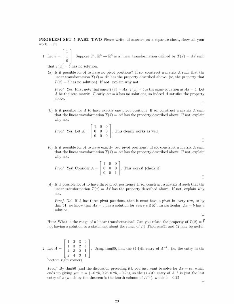
PROBLEM SET 5 PART TWO Please write all answers on a separate sheet, show all yourwork, ...etc

1. Let ~b =

110

. Suppose T : R3 → R3 is a linear transformation defined by T (~x) = A~x such

that T (~x) = ~b has no solution.

(a) Is it possible for A to have no pivot positions? If so, construct a matrix A such that thelinear transformation T (~x) = A~x has the property described above. (ie, the property that

T (~x) = ~b has no solution). If not, explain why not.

Proof. Yes. First note that since T (x) = Ax, T (x) = b is the same equation as Ax = b. LetA be the zero matrix. Clearly Ax = b has no solutions, so indeed A satisfies the propertyabove.

(b) Is it possible for A to have exactly one pivot position? If so, construct a matrix A suchthat the linear transformation T (~x) = A~x has the property described above. If not, explainwhy not.

Proof. Yes. Let A =

1 0 00 0 00 0 0

. This clearly works as well.

(c) Is it possible for A to have exactly two pivot positions? If so, construct a matrix A suchthat the linear transformation T (~x) = A~x has the property described above. If not, explainwhy not.

Proof. Yes! Consider A =

1 0 00 0 00 0 1

. This works! (check it)

(d) Is it possible for A to have three pivot positions? If so, construct a matrix A such that thelinear transformation T (~x) = A~x has the property described above. If not, explain whynot.

Proof. No! If A has three pivot positions, then it must have a pivot in every row, so bythm 51, we know that Ax = c has a solution for every c ∈ R3. In particular, Ax = b has asolution.

Hint: What is the range of a linear transformation? Can you relate the property of T (~x) = ~bnot having a solution to a statement about the range of T? Theorems51 and 52 may be useful.

2. Let A =

1 2 3 41 3 2 44 3 2 12 4 3 1

. Using thm80, find the (4,4)th entry of A−1. (ie, the entry in the

bottom right corner)

Proof. By thm80 (and the discussion preceding it), you just want to solve for Ax = e4, whichends up giving you x = (−0.25, 0.25, 0.25,−0.25), so the (4,4)th entry of A−1 is just the lastentry of x (which by the theorem is the fourth column of A−1), which is −0.25

23

3. Suppose T : R3 → R3 is a linear transformation such that

T (~e1) =

111

and T (~e2) =

222

(a) Can T be 1-1? If yes, give an example of a T that is both 1-1 and satisfies the properties

described above. If no, explain why.Hint: If you said yes, then the easiest way to define a linear transformation is to come upwith a matrix A, and define T (~x) = A~x. Note that here, the matrix will have to be 3× 3.Hint: Recall the definition of 1-1 (50), and linear transformation (40).

Proof. Nope! Let A be the standard matrix for T . Note that the two conditions aboveimply that the first two columns of A are T (e1), T (e2). Ie, A must have the form

A =

1 2 a1 2 b1 2 c

But no matter what the last column contains, the first two columns are linearly dependent,so all three columns must be linearly dependent! (the first column is a linear combinationof the second one, and hence also a linear combination of the second and third columns).Thus, by thm54, T cannot be 1-1.

(b) Can T be onto? If yes, give an example. If no, explain why.Hint: As usual, when asked if something can be/is onto, theorem51 will be useful.

Proof. From above, we know that T cannot be 1-1, and hence since T is square, by thm94,it can’t be onto either.

(c) Is the set {~e1, ~e2} linearly independent? Is the set {T (~e1), T (~e2)} linearly independent?

Proof. Yes to the first question, no to the second.

(d) Suppose:

T

111

=

444

and ~w =

12−3

Compute T (~w).

Proof. First, write w as a linear combination of

111

, e1, and e2. In other words, find

x1, x2, x3 such that 12−3

= x1

100

+ x2

010

+ x3

111

Then use linearity of T to compute

T

12−3

= x1T

100

+ x2T

010

+ x3T

111

But you know all the values on the right hand side of the above equation, so you cancompute this for yoself.

24

11. Lecture 11. (Section 2.3) Exam and review session details on

http://www.math.psu.edu/dmh/Teaching/Fall2011-220/

– REVIEW Session on Sunday, 10/9 starting at 6pm in 117 Osmond

– EXAM on Wednesday, 10/12 from 6:30 - 7:45pm in 102 Forum

– CONFLICT Exam on Wednesday, 10/12 from 5:05 - 6:20pm in 108 Tyson

– MAKEUP Exam on Thursday, 10/20 from 6:30 - 7:45pm ...somewhere else

So far we’ve discussed what it means for linear transformations to be onto and 1-1, what it meansfor their standard matrices, and how you can tell. Today, we summarize the results we’ve uncovered,and derive some new implications.

Recall:

Theorem 83. (From 48) Let T : Rn → Rm be a linear transformation, then there is a uniquematrix AT such that T (x) = ATx for all x ∈ Rn. In fact, AT = [T (e1) T (e2) . . . T (en)]. We callthis matrix AT the (standard) matrix for T .

Firstly, many problems will require you to determine if a particular linear transformation is 1-1/onto.If the transformation is defined in terms of its matrix, then the table below gives you a concreteway to tell if the transformation is 1-1/onto. If it isn’t, then just find its matrix! (and then use thetable).

Suppose T : Rn → Rm is a linear transformation, and let A be its matrix, then

T is onto T is not ontoT is 1-1 Every row and column Every column of A has a

of A has a pivot. pivot, but not every row.T is not 1-1 Every row of A has a There are both columns and

pivot, but not every column. rows without pivots.

The above table tells us what 1-1/onto mean in terms of what the matrix of the transformationmust look like, but often it is also necessary to understand the other consequences of a lineartransformation being 1-1/onto. The most important ones are summed up here:

Theorem 84. (From51)Let T : Rn → Rm be a linear transformation with matrix A. The followingare equivalent:

(a) T is onto.

(b) For every b ∈ Rm, the equation Ax = b has a solution.

(c) Every row of A has a pivot.


Theorem 85. (From54) Let T : Rn → Rm be a linear transformation with standard matrix A. Thefollowing are equivalent:

(a) T is 1-1.

(b) The equation Ax = 0 has a unique solution.

(c) Every column of A has a pivot.

(d) The columns of A are linearly independent.

Exercise 86. Suppose T : R2 → R2 is a linear transformation given by T (x, y) = (2x − y, x + y),then is T 1-1? Is T onto?

25

Note that in the above exercise, after we discovered that T is 1-1, we automatically know for freethat T is onto! This is because any square matrix with a pivot in every column must also have apivot in every row (and vice versa).

Before stating the following result, we need a quick discussion on invertible transformations.

Definition 87. Define idn : Rn → Rn to be the linear transformation defined by:

idn(x) = x for all x ∈ Rn

Definition 88. A linear transformation T : Rn → Rm is said to be an invertible linear transforma-tion if there exists another linear transformation S : Rm → Rn such that

(a) For all x ∈ Rn, S(T (x)) = x.

(b) For all x ∈ Rm, T (S(x)) = x.

In this case, we call S the inverse of T , or T−1.

Note that the two conditions above say that S ◦ T = idn, and T ◦S = idm. (Recall that S ◦ T is thecomposition of S and T , which is a linear transformation defined by “first apply T , then apply S”.)

Pictorially, the situation above is as follows:

RnT**Rm

S

jj

where S, T are inverses of each other if S “undoes” everything that T does, and similarly T “undoes”everything that S does.

Note that this definition directly parallels the definition for a matrix inverse, which I’ve reproducedhere for convenience:

Definition 89. (From70) Let A be an n × n matrix, then A is said to be invertible if there existsan n× n matrix B with AB = BA = In. We call B the inverse of A, or A−1.

Example 90. Let T : R3 → R2 be given by T (x1, x2, x3) = (x1, x2), and S : R2 → R3 be given byS(x1, x2) = (x1, x2, 0). Note that T (1, 2, 0) = (1, 2), and S(1, 2) = (1, 2, 0).

(a) Are S, T inverses of each other? (ie, is T invertible with T−1 = S?)

The answer is no! Note that T maps (1, 2, 3) to (1, 2), but S maps (1, 2) to (1, 2, 0), so S doesnot reverse the action of T on all x.

(b) Is T invertible?

Again the answer is no! Let A be the standard matrix for T , then

T maps a large space into a small space =⇒ A have more columns than rows

⇐⇒ not every column of A contains a pivot

⇐⇒ T is not 1-1

⇐⇒ there exist distinct vectors x, y ∈ R3 such that T (x) = T (y)

Let z = T (x), then the last statement says that: “T maps distinct vectors x, y both to z”.

This means that for any function S to reverse the action of T on x, it must map z to x, andfor it to reverse the action of T on y, it must map z to y, but S can’t map z to both x and y(since S is a function!), so no such S exists, and T is not invertible.

So, WHY isn’t T invertible? Fundamentally, what went wrong was the fact that T is not 1-1. Thus,since T maps distinct vectors to the same vector, it “discards information”, and thus, given anyvector z in the codomain (here, R2), the vector in the domain (here, R3) that maps to z cannot berecovered, since it is not unique (there are multiple vectors in R3 that maps to z ∈ R2)

Thus, in general, if T is not 1-1, then T is not invertible. In particular, if n > m, then any mapT : Rn → Rm cannot be 1-1, hence is not invertible.

26

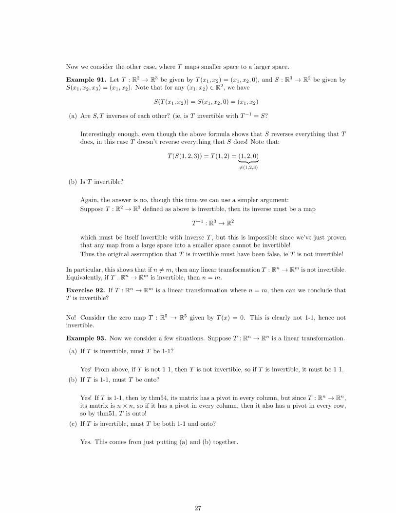
Now we consider the other case, where T maps smaller space to a larger space.

Example 91. Let T : R2 → R3 be given by T (x1, x2) = (x1, x2, 0), and S : R3 → R2 be given byS(x1, x2, x3) = (x1, x2). Note that for any (x1, x2) ∈ R2, we have

S(T (x1, x2)) = S(x1, x2, 0) = (x1, x2)

(a) Are S, T inverses of each other? (ie, is T invertible with T−1 = S?

Interestingly enough, even though the above formula shows that S reverses everything that Tdoes, in this case T doesn’t reverse everything that S does! Note that:

T (S(1, 2, 3)) = T (1, 2) = (1, 2, 0)︸︷︷︸6=(1,2,3)

(b) Is T invertible?

Again, the answer is no, though this time we can use a simpler argument:

Suppose T : R2 → R3 defined as above is invertible, then its inverse must be a map

T−1 : R3 → R2

which must be itself invertible with inverse T , but this is impossible since we’ve just proventhat any map from a large space into a smaller space cannot be invertible!

Thus the original assumption that T is invertible must have been false, ie T is not invertible!

In particular, this shows that if n 6= m, then any linear transformation T : Rn → Rm is not invertible.Equivalently, if T : Rn → Rm is invertible, then n = m.

Exercise 92. If T : Rn → Rm is a linear transformation where n = m, then can we conclude thatT is invertible?

No! Consider the zero map T : R5 → R5 given by T (x) = 0. This is clearly not 1-1, hence notinvertible.

Example 93. Now we consider a few situations. Suppose T : Rn → Rn is a linear transformation.

(a) If T is invertible, must T be 1-1?

Yes! From above, if T is not 1-1, then T is not invertible, so if T is invertible, it must be 1-1.

(b) If T is 1-1, must T be onto?

Yes! If T is 1-1, then by thm54, its matrix has a pivot in every column, but since T : Rn → Rn,its matrix is n × n, so if it has a pivot in every column, then it also has a pivot in every row,so by thm51, T is onto!

(c) If T is invertible, must T be both 1-1 and onto?

Yes. This comes from just putting (a) and (b) together.

27

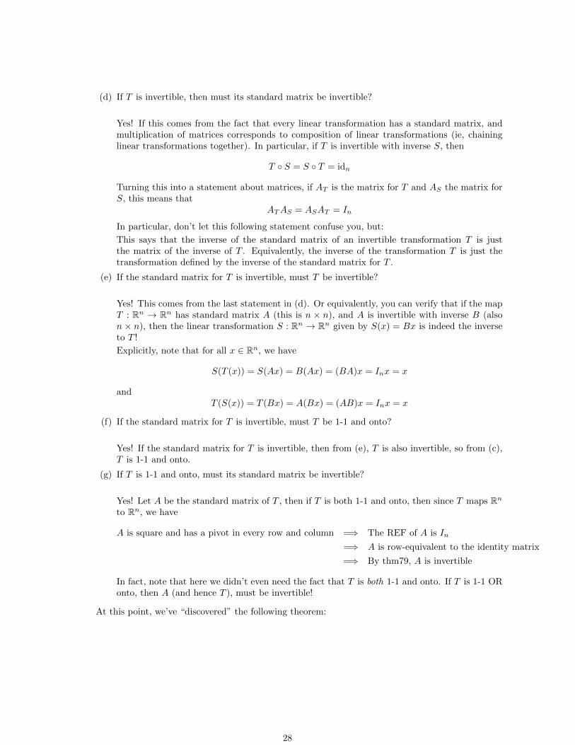
(d) If T is invertible, then must its standard matrix be invertible?

Yes! If this comes from the fact that every linear transformation has a standard matrix, andmultiplication of matrices corresponds to composition of linear transformations (ie, chaininglinear transformations together). In particular, if T is invertible with inverse S, then

T ◦ S = S ◦ T = idn

Turning this into a statement about matrices, if AT is the matrix for T and AS the matrix forS, this means that

ATAS = ASAT = In

In particular, don’t let this following statement confuse you, but:

This says that the inverse of the standard matrix of an invertible transformation T is justthe matrix of the inverse of T . Equivalently, the inverse of the transformation T is just thetransformation defined by the inverse of the standard matrix for T .

(e) If the standard matrix for T is invertible, must T be invertible?

Yes! This comes from the last statement in (d). Or equivalently, you can verify that if the mapT : Rn → Rn has standard matrix A (this is n × n), and A is invertible with inverse B (alson× n), then the linear transformation S : Rn → Rn given by S(x) = Bx is indeed the inverseto T !

Explicitly, note that for all x ∈ Rn, we have

S(T (x)) = S(Ax) = B(Ax) = (BA)x = Inx = x

andT (S(x)) = T (Bx) = A(Bx) = (AB)x = Inx = x

(f) If the standard matrix for T is invertible, must T be 1-1 and onto?

Yes! If the standard matrix for T is invertible, then from (e), T is also invertible, so from (c),T is 1-1 and onto.

(g) If T is 1-1 and onto, must its standard matrix be invertible?

Yes! Let A be the standard matrix of T , then if T is both 1-1 and onto, then since T maps Rn

to Rn, we have

A is square and has a pivot in every row and column =⇒ The REF of A is In

=⇒ A is row-equivalent to the identity matrix

=⇒ By thm79, A is invertible

In fact, note that here we didn’t even need the fact that T is both 1-1 and onto. If T is 1-1 ORonto, then A (and hence T ), must be invertible!

At this point, we’ve “discovered” the following theorem:

28

Theorem 94. Let T : Rn → Rn be a linear transformation with matrix A. The following areequivalent:

(a) T is invertible.

(b) A is invertible.

(c) T is 1-1 and onto.

(d) T is 1-1.

(e) T is onto.

Furthermore, any linear transformation T : Rn → Rm for n 6= m is not invertible, and similarly anymatrix that is not square is not invertible.

Note that this theorem is compatible with theorems 51 and 54:

Example 95. Suppose T : Rn → Rn is a linear transformation, and suppose T (x) = b has a solutionfor every b ∈ Rn, then is T 1-1? onto? invertible?

All three are true! Let A be its standard matrix, then to say that T (x) = b has a solution for everyb ∈ Rn is to say that Ax = b has a solution for every b ∈ Rn, which by thm51, we see that thismeans that T is onto, and hence (by thm94) T is 1-1, onto, and invertible!

Exercise 96. (Seriously, do this!) Let T : R2 → R2 be defined by T (x1, x2) = (2x1+x2, 5x1+3x2).

(a) Find the standard matrix for T . Call it A. Note that as usual, for all x ∈ R2, we haveT (x) = Ax (ie, this gives an equivalent description of T )

(b) Verify that the matrix A found in (a) is an invertible matrix, and find its inverse, which we’llcall B.

(c) Define the linear transformation S : R2 → R2 by S(x) = Bx.

(d) Verify that S and T are inverses of each other (ie, T is invertible with inverse S and vice versa)

(e) Find the standard matrices of S and T . (You’ve done most of the work already)

(f) Verify that the standard matrices of S and T are inverses of each other.

Other random questions:

– What’s the standard matrix for scale vertically by 2? (as a transformation from R2 → R2)

– What’s the standard matrix for reflect across the origin?

– What’s the standard matrix for “scale vertically by 2, then reflect across the origin”?

– What’s its inverse?

– Suppose T : R3 → R3 is a linear transformation, and suppose there are distinct vectors u, vsuch that T (u) = T (v). What can you say about T? What can you say about its matrix?What if u, v were LI? What now?

– Suppose T (1, 0) = (3, 3, 8), and T (0, 1) = (1, 0, 1). What is T (−1, 5)?

– Let T : R3 → R3, and T (1,−2, 3) = (1, 1, 1), T (2,−1, 0) = (1, 6, 2), and T (5, 2, 1) = (−1,−1,−1).What is T (10, 10, 10)? Is there enough information? What is the range of T?

– Let T : Rn → Rm be linear. If T is 1-1, what can you say about n,m? If T is onto, what canyou say about n,m? What is T (0)?

– Let T be defined by T (x, y, z) = (2x+ y, x+ 2y, y− z). Is it 1-1? Is it onto? How do you solvethis? What is its matrix?

29

12. Lecture 12. (Sections 2.3 and 2.8)

HOMEWORK DUE NOW!

Quiz at end of class. Three problems, 6 points per problem, and 2 bonus points for finishing ontime.

Finishing up invertible matrices. Now that we’ve talked enough about how matrices can bemanipulated, it’s valuable to spend a moment to think about doing algebra with matrices. In fact,you can do algebra much the same way, keeping in mind the warnings from 66

Example 97. Suppose A,B are invertible n× n matrices.

(a) Is AB invertible?

Yes! This was discussed earlier. In fact, the inverse is just B−1A−1.

(b) Is A+B? Invertible?

No! (not in general). For example, consider I and −I. Clearly both I, −I are invertible, butI + (−I) = 0.

(c) Suppose A(C +D) = B, then is C +D invertible?

Yes! Note that since A is invertible, we can multiply both sides on the left by A−1, giving us:C +D = A−1B, but A−1, B are both invertible, so A−1B is invertible, hence C +D is.

(d) Suppose C,D are also n×n matrices, though not necessarily invertible, and A(X+C)B−1 = D.Can we solve for X?

Yes! Proceed as you would normally do, keeping in mind that you have to multiply on thesame side when manipulating the equation.

A(X + C)B−1 = D

(X + C)B−1 = A−1D

X + C = A−1DB

X = A−1DB − C

Subspaces.

First, recall the definition of a vector space. Really, you don’t need to remember all the technicaldetails word-for-word, but the idea you should have in your mind is that a vector space is “a setwhere you can add and scale” where also the set must have a 0 element, as well as “negative”elements.

Until now, the only examples of vector spaces that we’ve discussed in detail are the sets Rn. Whilethe category of vector spaces is far more diverse than just Rn, today we’ll expand our bank ofexamples of vector spaces to subspaces of Rn.

Definition 98. Let V be a vector space, then a subset W ⊆ V is a subspace if W is itself a vectorspace.

Theorem 99. A subset W ⊆ V is a subspace if and only if

(a) For all u, v ∈W , u+ v ∈W(b) For all u ∈W,a ∈ R, au ∈W .

30

We won’t prove this, but intuitively, this means that a subset W of a vector space is a vector spaceif and only if the sum of any two things in W is also in W , and any scalar multiple of anything inW is also in W .

(For the purpose of a definitions quiz, I’ll allow this theorem to be cited as an “alternate” definitionof subspace)

Example 100.

(a) Let V be a vector space. Must every subspace of V contain 0 (the zero vector)?

Yes! Let W be any subspace of V , and let u be any vector in W . By property (b) of 99, sinceu ∈W , we must have 0u ∈W , but 0u = 0, so 0 ∈W . This gives a quick check to see if certainsubsets are not subspaces (ie, if you’re given a subset of a vector space that doesn’t have 0, itcan’t be a subspace!)

(b) Let v1, . . . , vp ∈ Rn, then is Span {v1, . . . , vp} a subspace?

Yes! Any sum of linear combinations of v1, . . . , vp is a linear combination, and so is any scalarmultiple. We discussed this earlier. Explicitly, if ai, bi, c ∈ R, then

(a1v1 + a1v2 + · · ·+ apvp) + (b1v1 + b2v2 + · · ·+ bpvp) = (a1v1 + b1v1) + · · ·+ (apvp + bpvp)

= (a1 + b1)v1 + · · ·+ (ap + bp)vp

andc(a1v1 + a1v2 + · · ·+ apvp) = (ca1)v1 + · · ·+ (cap)vp

(c) What about the line x = y in R2?

Yes! This is just Span {(1, 1)}, or equivalently Span {(2, 2)},Span {−6,−6}, or in generalSpan {(a, a)} for any a 6= 0.

(d) Consider Span {(1, 1, 1), (1, 2, 3)} ⊆ R3. Now suppose we add a vector v into the span. Forwhat v will Span {(1, 1, 1), (1, 2, 3), v} 6= Span {(1, 1, 1), (1, 2, 3)}?

Well, if it doesn’t change the span, that means that v must have already been in Span {(1, 1, 1), (1, 2, 3)},ie, {(1, 1, 1), (1, 2, 3), v} is linearly dependent!

On the other hand, if it does change the span, then in fact the set {(1, 1, 1), (1, 2, 3), v} willbe linearly independent. You can prove this by showing that none of the vectors can be linearcombinations of the others, though by next thursday we’ll have a slicker way to argue this.

Recall that the range of a linear transformation T : Rn → Rm is just the span of the columns of itsstandard matrix. Now, we’ll give this space a name:

Definition 101. The column space of a matrix A is the span of its columns, denoted Col A.

Note that while “range” is a word that applies to functions, “column space” is a word that applies toa matrix. The connection between these two terms is as follows: “the range of a linear transformationT is the column space of the standard matrix for T”

Example 102. Let A be an m× n matrix. Is Col A a subspace? What is it a subspace of?

Yup! By definition, it’s the span of a bunch of vectors, hence is a subspace! Since the vectors are inRm, it’s a subspace of Rm.

Definition 103. The null space of a matrix A is the solution set of Ax = 0, denoted Nul A.

Example 104.

31

(a) Let A be m× n. Is Nul A a subspace? What is it a subspace of?

Yes again! Firstly, if u ∈ Nul A, then Au = 0, so for this to make sense, we must have u ∈ Rn,so Nul A is a subset of Rn.

To see that it’s a subspace, suppose u, v ∈ Nul A, then that’s to say that Au = Av = 0, but thenA(u+v) = Au+Av = 0, so u+v ∈ Nul A. Furthermore, if c ∈ R, then A(cu) = c(Au) = c0 = 0,so cu ∈ Nul A, so by 99, Nul A is a subspace (of Rn).

(b) Now let A be an m× n matrix, and b ∈ Rm with b 6= 0. Let W be the solution set of Ax = b.Is W a subspace?

No! Recall that the solution set of Ax = b is either empty, or a shifted copy of the solution setof Ax = 0 (which we now can call Nul A). Thus, if Ax = b is consistent and p is any solutionto Ax = b, then [

Solution set of Ax = b]

= {p+ w : w ∈ Nul A}

Now, does the right hand side contain 0?

Geometrically speaking, you can imagine that the solution set of Ax = 0 (ie, Nul A) is goingto be some line, plane, or higher dimensional space through the origin, and the solution set ofAx = b is some shifted copy of that. But since it shifts in a direction that is not “along” theline/plane, the shifted copy won’t contain 0. (Note that shifting the line x = y by the vector(1,1) will not change the line at all!)

However, this is not a proof. To prove this, we have to appeal to the algebra:

Algebraically speaking, if 0 = p+ w for some w ∈ Nul A, then p = −w, so since this expressesp as a scalar multiple of something in Nul A, using the fact that Nul A is a subspace, we canconclude that p ∈ Nul A.

However, this is impossible, since by assumption Ap = b and b 6= 0, so p /∈ Nul A, so we cannotwrite 0 = p+ w for any w ∈ Nul A, ie 0 is not in the solution set of Ax = b.

The following definition is kind of the most important idea in all of linear algebra.

Definition 105. A basis for a vector space is a linearly independent subset of W that spans W .

32

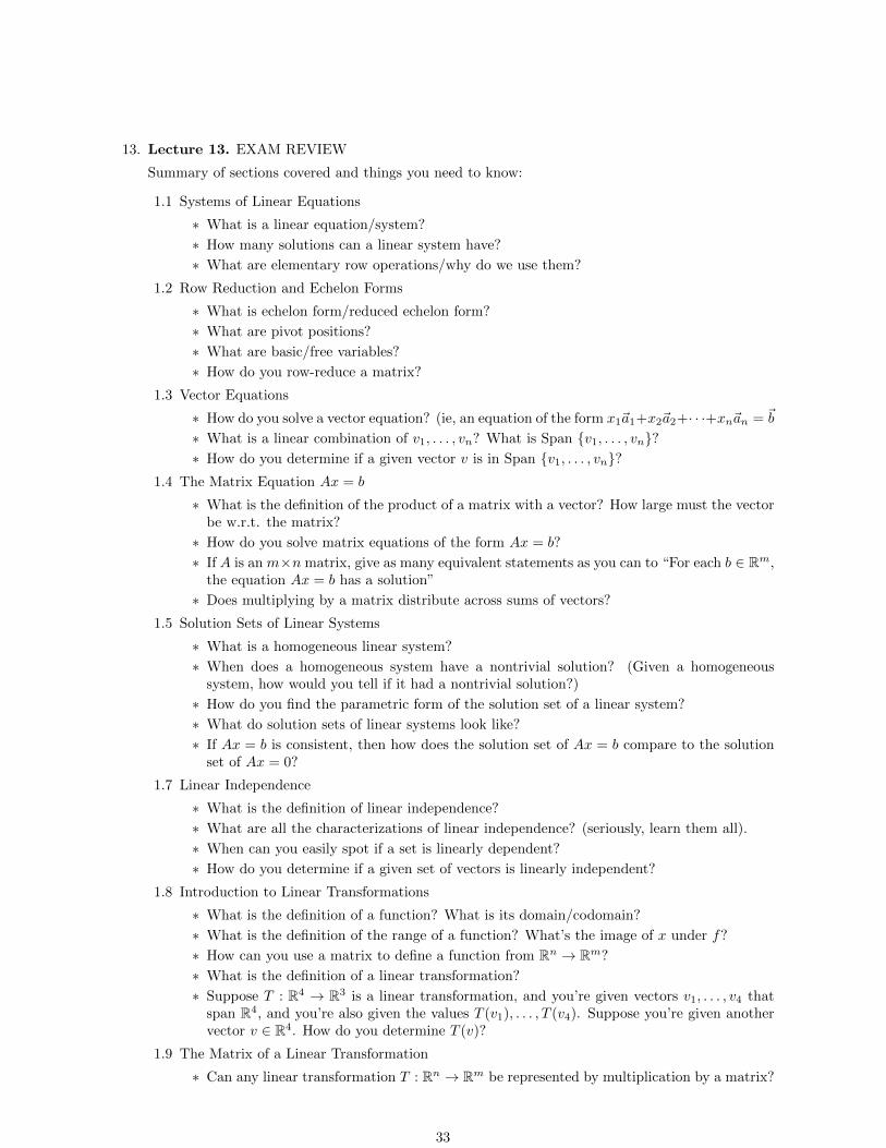
13. Lecture 13. EXAM REVIEW

Summary of sections covered and things you need to know:

1.1 Systems of Linear Equations

∗ What is a linear equation/system?

∗ How many solutions can a linear system have?

∗ What are elementary row operations/why do we use them?

1.2 Row Reduction and Echelon Forms

∗ What is echelon form/reduced echelon form?

∗ What are pivot positions?

∗ What are basic/free variables?

∗ How do you row-reduce a matrix?

1.3 Vector Equations

∗ How do you solve a vector equation? (ie, an equation of the form x1~a1+x2~a2+· · ·+xn~an = ~b

∗ What is a linear combination of v1, . . . , vn? What is Span {v1, . . . , vn}?∗ How do you determine if a given vector v is in Span {v1, . . . , vn}?

1.4 The Matrix Equation Ax = b

∗ What is the definition of the product of a matrix with a vector? How large must the vectorbe w.r.t. the matrix?

∗ How do you solve matrix equations of the form Ax = b?

∗ If A is an m×n matrix, give as many equivalent statements as you can to “For each b ∈ Rm,the equation Ax = b has a solution”

∗ Does multiplying by a matrix distribute across sums of vectors?

1.5 Solution Sets of Linear Systems

∗ What is a homogeneous linear system?

∗ When does a homogeneous system have a nontrivial solution? (Given a homogeneoussystem, how would you tell if it had a nontrivial solution?)

∗ How do you find the parametric form of the solution set of a linear system?

∗ What do solution sets of linear systems look like?

∗ If Ax = b is consistent, then how does the solution set of Ax = b compare to the solutionset of Ax = 0?

1.7 Linear Independence

∗ What is the definition of linear independence?

∗ What are all the characterizations of linear independence? (seriously, learn them all).

∗ When can you easily spot if a set is linearly dependent?

∗ How do you determine if a given set of vectors is linearly independent?

1.8 Introduction to Linear Transformations

∗ What is the definition of a function? What is its domain/codomain?

∗ What is the definition of the range of a function? What’s the image of x under f?

∗ How can you use a matrix to define a function from Rn → Rm?

∗ What is the definition of a linear transformation?

∗ Suppose T : R4 → R3 is a linear transformation, and you’re given vectors v1, . . . , v4 thatspan R4, and you’re also given the values T (v1), . . . , T (v4). Suppose you’re given anothervector v ∈ R4. How do you determine T (v)?

1.9 The Matrix of a Linear Transformation

∗ Can any linear transformation T : Rn → Rm be represented by multiplication by a matrix?

33

∗ Given a linear transformation T : Rn → Rm, how do you find the matrix A such thatT (x) = Ax for all x ∈ Rn?

∗ Come up with some 2× 2 matrices and describe their action on the plane.

∗ What does it mean for a function to be onto? 1-1?

∗ Come up with as many equivalent statements as you can to “a linear transformation T :Rn → Rm is 1-1”

∗ Come up with as many equivalent statements as you can to “a linear transformation T :Rn → Rm is onto”

2.1 Matrix Operations

∗ When is the product of two matrices defined/undefined?

∗ What’s the definition of the product of two matrices AB?

∗ What’s the row-column rule for computing matrix products?

∗ What is the significance of the product of two matrice AB w.r.t. the linear transformationsthey represent?

∗ Is AB = BA for all matrices A,B (of the appropriate sizes) ?

∗ If AB = AC, then does that mean B = C?

∗ If AB = 0, must A = 0 or B = 0?

∗ Given an equation involving matrices like A(I+X)B = D how can you solve for X? (Whenis it possible?)

∗ What is the transpose of a matrix? What are the properties of the transpose?

2.2 The Inverse of a Matrix

∗ What does it mean for a matrix to be invertible?

∗ When is a 2× 2 matrix invertible?

∗ If A is invertible, then what does that say about the equation Ax = b?

∗ If A,B are invertible, what is the inverse of AB?

∗ What is an elementary matrix?

∗ What must the REF of an invertible matrix look like?

∗ How can you tell if a matrix is invertible? If it is, how do you find its inverse?

∗ How can you compute a particular column of the inverse without computing the entireinverse?

2.3 Characterzations of Invertible Matrices

∗ If m 6= n, and A is m× n, can A be invertible?

∗ If A is square, come up with as many equivalent statements as you can to “A is invertible”

∗ What is an invertible linear transformation?

∗ If T : Rn → Rn is invertible, how would you find its inverse?

2.8 Subspaces of Rn

∗ What is a subspace of Rn?

∗ What is the column space/null space of a matrix?

∗ What is a basis for a vector space?

34

14. Lecture 14. (Sections 2.8, 2.9) Definitions quiz next thursday.

Recall the definition of basis:

Definition 106. A basis for a vector space W is a linearly independent subset of W that spans W .

I’ve cut/pasted these examples from last time:

Example 107.

(a) Conisder the set {e1, e2} ⊆ R2. Is this a basis for R2?

Yes. To verify this, we have to check that it’s both (a) linearly independent, and (b) spans allof R2. It’s easy to check this by elementary means, but we’re going to do something else:

Consider the matrix I2 = [ 1 00 1 ]. Since it’s clearly got a pivot in every column, by 54, the

columns (which are e1, e2) are linearly independent. Since it’s clearly got a pivot in every row,by 51, the columns span all of R2.

We used this method because it is easily generalizable.

(b) Consider the set {(−2, 0, 4), (1, 2, 3), (2, 2, 1)}. Is this a basis for R3?

As it turns out, no! Even though you can’t spot any obvious relations between the three, itturns out that the set is in fact linearly dependent, and hence does not span R3. To see this,consider the matrix with those three vectors as columns. As it turns out...

A =

−2 1 20 2 24 3 1

∼ 1 0 −1/2

0 1 10 0 0

And thus since there isn’t a pivot in the last row/column, the columns are not linearly inde-pendent, AND the columns do not span R3.

(c) Do the columns of the above matrix span R2?

NO! This is a favorite question to ask on the exam. R2 and R3 are completely different sets.While we might think of R2 as being “smaller” than R3, it is in no way a subset of R3. Thus,since the columns are vectors in R3, and the span of vectors in R3 give subspaces of R3, theanswer is a resounding NO.

(d) Let u, v, w ∈ R231, and let W = Span {u, v, w} ⊆ R231. Suppose {u, v, w} is linearly indepen-dent. Is {u, v, w} a basis for W?

Yes. By definition they span W , and by assumption they’re linearly independent, so they’re abasis for W !

They however are not a basis for R231.

Now that we’re comfortable checking to see if particular sets of vectors form a basis for Rn,let’s try to find a basis for some subspaces of Rn.

(e) Find a basis for the null space of the matrix

A =

−3 6 −1 1 −71 −2 2 3 −12 −4 5 8 −4

To do this, we’ll want to write the solution of Ax = 0 in parametric vector form.

[A 0] ∼

1 −2 0 −1 3 00 0 1 2 −2 00 0 0 0 0 0

−→ x1 − 2x2 − x4 + 3x5 = 0x3 + 2x4 − 2x5 = 0

0 = 0

35

Writing the basic variables in terms of the free variables, we get:

x1 = 2x2 + x4 − 3x5

x3 = −2x4 + 2x5

Thus, a general solution will look like:x1x2x3x4x5

=

2x2 + x4 − 3x5

x2−2x4 + 2x5

x4x5

= x2

21000

︸︷︷︸

u

+x4

10−2

10

︸︷︷︸

v

+x5

−3

0201

︸︷︷︸

w

Note here that the matrix [u v w] is already in echelon form, and in fact has a pivot inevery column! This tells us that {u, v, w} is linearly independent. On the other hand, thiscomputation shows us that Nul A is exactly Span {u, v, w}.

In example (e) above, in general the matrix [u, v, w] may not be in echelon form. On the otherhand, it is {u, v, w} will always be linearly independent. To see this, note that each vector u, v, wcorresponds to a free variable. In this case, u corresponds to x2, v to x4, and w to x5. Note that uis the only vector of the 3 that has a nonzero entry in the x2 position, and similarly for v with x4,and w with x5. Thus, if

x2u+ x4v + x5w = 0

this means that in particular the sums of the 2nd, 4th, and 5th coordinates of (x2u+ x4v+ x5w arezero, but since the only possible contributor to the 2nd coordinate is u, and v for the 4th, and w forthe 5th, we see that each coefficient x2, x4, x5 must all be 0.

Example 108. Consider the REF matrix

A =

1 0 2 0 −30 1 6 0 50 0 0 1 60 0 0 0 0

How can you describe Col A? What is a basis for Col A?

Clearly the span of the columns of A will only contain vectors with a 0 in the 4th coordinate.However, looking at the pivot columns, we see that any vector with a 0 in the 4th coordinate canbe expressed as a linear combination of the columns. Furthermore, the pivot columns are obviouslylinearly independent, so in this case we see that they form a basis for Col A.

Now consider

B =

2 0 4 0 −61 1 8 1 20 1 6 0 51 0 2 1 3

It can be shown that B ∼ A, ie A is the REF of B. But the column space of B is clearly differentfrom that of A, since it contains stuff with nonzero 4th coordinate. Indeed, Col B is much moredifficult to understand and coming up with a basis for Col B is also not easy.

Can anyone think of a way to find a basis for Col B?

In our efforts to understand Col B, we’ll need to discuss some further properties of linear transfor-mations.

36

Lemma 109. Suppose v is a linear combination of {v1, . . . , vp}, and T : V →W a linear transfor-mation, then T (v) is a linear combination of T (v1), . . . , T (vp).

Proof. Suppose v = a1v1 + · · ·+ apvp, then T (v) = T (a1v1 + · · ·+ apvp) = a1T (v1) + · · ·+ apT (vp).

Lemma 110. Suppose {v1, . . . , vp} is a linearly independent set, and T : V → W is a 1-1 lineartransformation, then {T (v1), . . . , T (vp)} is also linearly independent.

Proof. Suppose {T (v1), . . . , T (vp)} were linearly dependent, then there would be scalars a1, . . . , ap ∈R, not all 0, such that

a1T (v1) + · · ·+ apT (vp) = 0

But that means T (a1v1 + · · · + apvp) = 0. Since T is 1-1, this means that a1v1 + · · · + apvp = 0,which is to say that v1, . . . , vp were linearly dependent (since not all the ai’s are 0). Since v1, . . . , vpwere not linearly dependent, T (v1), . . . , T (vp) couldn’t have been linearly dependent either!

Now we can prove the following theorem, which tells us exactly how to find a basis for Nul A andCol A of any matrix A.

Theorem 111. Given an m× n matrix A

(a) The vectors obtained in the parametric form of the solution to Ax = 0 form a basis for Nul A.

(b) The pivot columns of A form a basis for Col A.

Proof. Only the second part remains to be proven.

To see that the pivot columns of A form a basis, we must prove two things:

To see that they are linearly independent, let B be the REF of A. Then for some elementary matricesE1, . . . , Ek, we have (Ek · · ·E1)A = B. Let E = Ek · · ·E1.

Clearly the pivot columns of B are linearly independent (think about what the pivot columns of amatrix in REF must look like), but also, since E1, . . . , Ek are invertible, so is E, so we have

EA = B A = E−1B

But letting b1, . . . , bn be the columns of B, we have E−1B = [E−1b1 . . . E−1bn], so the pivotcolumns of A are just E−1 times the pivot columns of B, so by lemma 110, the pivot columns of Aare also linearly independent.

Furthermore, they span the column space because:

(a) The non-pivot columns of B are linear combinations of the pivot columns of B.

(b) The non-pivot columns of A are just E−1 times the non-pivot columns of B, and thus by 109are linear combinations of the pivot columns of A.

In other words. Suppose b1, . . . , br are the pivot columns of B, and br+1, . . . , bn are the non-pivotcolumns, and similarly a1, . . . , ar are the pivot columns of A, and ar+1, . . . , an the non-pivotcolumns of A. (in general the pivot columns might not come first, but it doesn’t matter forthis argument)

Then, we know that for each i = 1, . . . , n, we have ai = E−1bi. Remark (a) tells us that foreach i = r + 1, . . . , n, we have bi is a linear combination of b1, . . . , br. Since multiplicationby E−1 is a linear transformation, so by 109, we also have that each ai = E−1bi is a linearcombination of a1 = E−1b1, . . . , ar = E−1br.

37

Coordinate Systems

Theorem 112. Suppose B = {b1, . . . , bp} is a basis for a vector space V , then for any x ∈ V , thereexist uniquely determined a1, . . . , ap ∈ R such that x = a1b1 + · · ·+ apbp.

Proof. Since a basis must span V , clearly such a1, . . . , ap exist. Now suppose there c1, . . . , cp ∈ Ralso has the property that x = c1b1 + · · ·+ cpbp, then subtracting, we get:

0 = x− x = (a1 − c1)b1 + · · ·+ (ap − cp)bp

but since the b1, . . . , bp are linearly independent, all the coefficients on the right hand side of theabove equation are zero, ie ai = ci for each i.

Definition 113. Two vector spaces V,W are called isomorphic if there is an invertible linear trans-formation T : V →W . We write V ∼= W to mean V is isomorphic to W .

Theorem 114. Suppose B = {b1, . . . , bn} is a basis for V ⊆ Rm, then V ∼= Rn.

Proof. Define a linear transformation T : Rn → V by sending ei 7→ bi, ie

T (a1e1 + · · ·+ anen) = a1b1 + · · ·+ anbn for all ai ∈ R

Now, this is 1-1, since the standard matrix of T (viewed as a linear transformation Rn → Rm) isjust A = [T (e1) T (e2) · · · T (en)] = [b1 b2 · · · bn], but since b1, . . . , bn are a basis, they’re linearlyindependent, so the standard matrix must represent a 1-1 transformation.

Furthermore, it’s onto, since V = Span {b1, . . . , bn}, but clearly T will map to any linear combinationof the bi’s, so T is onto.

Note that we also have a map T−1 : V → Rn given by

T−1(a1b1 + · · ·+ anbn) = a1e1 + · · ·+ anen =

a1...

an

This map essentially gives us a way of writing vectors of V as vectors of Rn.

Note. In the proof above, note that if we think of T as a linear transformation Rn → Rm, it’s notonto, but if we restrict the codomain to V ⊆ Rm, it is onto!

Indeed, this fact is reflected in the following question: Must the matrix A defined above be invertible?

Nope! Note that A is m× n, so if m 6= n, A isn’t invertible!

In a way, the above theorem says that we can work with V in essentially the same way as workingwith Rn. Concretely speaking, we need a good way of representing vectors in V :

Definition 115. Suppose the set B = {b1, . . . , bp} is a basis for a vector space V , then for eachx ∈ V , the coordinates of x relative to the basis B are the coefficients c1, . . . , cp such that

x = c1b1 + · · ·+ cpbp

The vector:

[x]B =

c1...cp

is called the coordinate vector of x relative to B, or the B-coordinate vector of x.

38

15. Lecture 15. (Section 2.9) DEFINITIONS QUIZ ON THURSDAY

PROBLEM SET 6 DUE NEXT THURSDAY (start early. It’s long)

Example 116. Consider the vectors:

v =

112

, b1 =

110

, b2 =

001

(a) Are b1, b2 linearly independent? For what vector space V is B = {b1, b2} a basis?

Since B is linearly independent obviously B spans Span B, it’s a basis for Span B! Now,theorem 114 tells us that V must behave exactly like R2. How exactly does it behave like R2?

(b) Is v ∈ Span B? What is [v]B?

Yes, v = b1 + 2b2. By the definition, we have [v]B =

[12

]. Indeed, the map:

[·]B : Span B → R2

that takes any v ∈ Span B to [v]B ∈ R2 is really just the map T−1 defined in thm 114. Thisallows us to identify R2 with a subspace of R3.

In this way we can identify any vector space as Rn for some n.

(c) What I’m about to say is a little philosophical:

Consider all the points on the (infinite) blackboard. I’ll draw a special point called O, and I’lldefine the scalar multiple aP (a ∈ R) of a point P as just being the point Q that lies on thesame line as P and O, but is a-times as far away from O as P .

Furthermore, I’ll define the sum of points P +Q as the fourth point of the parallelogram withvertices at P,Q,O and edges PO,QO. Using these definitions, we can similarly define linearcombinations, span, linear independence, and so on.

Now, it can be shown geometrically that this is a vector space! But, clearly

B = {all points on the infinite blackboard} 6= {all lists of real numbers (x, y) with x, y ∈ R} = R2

They’re just completely different sets, in the sense that the set of all apples is different from theset of all oranges. However, they are similar in a certain sense, in that both apples and orangesare fruits, and so any knowledge we have of apples that depend only on their “fruitiness”carries over to the land of oranges. On the other hand, oranges are tasty and apples are gross,so they’re not all the same.

In the same sense, even though you can “erase” points on the blackboard, but you can’t eraselists of real numbers (since they’re in your head), these two sets are similar as vector spaces.Consider the following questions, and ask them of B and R2:

i. Is there a nonzero element?

ii. Does there exist an element x such that every element is a scalar multiple of x?

iii. Do there exist elements x, y such that every element is a linear combination of x, y?

We see that each question has the same answer for B and R2! Thus, in this sense, they aresimilar. On the other hand, for us it’s easier to add vectors in R2 than it is to add points bydrawing a parallelogram and finding the 4th vertex. Thus, we want a way of connecting B withR2 in a way that allows easy transition between the two worlds.

This ends up just amounting to putting a coordinate system on B. Pick any two linearlyindependent points P,Q ∈ B, and define the linear transformation

T : B→ R2 by T (aP + bQ) =

[ab

]

39

It can be shown (completely geometrically!) that P,Q are a basis for B, and so by thm114, wesee that T is both 1-1 and onto, and thus we can identify B with R2 via T .

The key point here is that you can put different coordinate systems on B by choosing differentpoints for P,Q.

(d) The fact that you can put different coordinate systems on any vector space is essentially whywe talk about the standard matrix for a linear transformation. You can represent the same lineartransformation via different matrices! In fact, given any linear transformation T : Rn → Rm and achoice of basis B for Rn and C for Rm, you can define a matrix A such that A[v]B = [T (v)]C .

Theorem 117. Let V be a vector space and let B = {b1, . . . , bn} and C = {c1, . . . , cm} be two basesfor V . Then n = m.

Proof. Suppose not, that, say, n < m, then we have invertible linear transformations S : Rn → Vand T : V → Rm, so T ◦S is an invertible linear transformation Rn → Rm, which is impossible fromour discussions on section 2.3.

Lemma 118. Suppose V is a vector space, and let {v1, . . . , vn} ⊆ V be linearly independent. Letw ∈ V with w /∈ Span {v1, . . . , vn}, then {w, v1, . . . , vn} is also linearly independent.

Proof. Suppose there exist a0, . . . , an ∈ R with a0w + a1v1 + · · · + anvn = 0. To show that{w, v1, . . . , vn} is linearly independent, we’d like to show that a0 = a1 = · · · = an = 0.

Now, first consider the case where a0 = 0. But that would mean that a1v1 + · · ·+ anvn = 0, so bylinear independence of {v1, . . . , vn}, we must have a1, . . . , an = 0, so it proves it in this case.

Now suppose a0 6= 0. Then, we can write

a0w = −a1v1 − · · · − anvn so... w = −a1a0v1 − · · · −

ana0vn

But this shows that w is a linear combination of v1, . . . , vn, which can’t happen because by assump-tion w /∈ Span {v1, . . . , vn}.

Theorem 119. Every vector space V has a basis.

Proof. The idea is to “grow” a basis starting with the set {v1} for u ∈ V any nonzero vector.

Let v1 ∈ V be any nonzero vector. If {v1} doesn’t form a basis, since it’s clearly linearly independent,it must be that {v1} doesn’t span V , so you can find something (call it v2) that lies outside Span {v1},and throw it in.

Now by the above lemma, we have that {v1, v2} is also linearly independent, so if {v1, v2} isn’t abasis, you can find v3 /∈ Span {v1, v2}, and consider {v1, v2, v3}.Continue in this way until your set spans V . (since at each step the set we have is linearly indepen-dent, the final set will be a basis for V )

Example 120. In this example we’ll try to come up with a good definition of dimension.

Now, it’s natural to think of R1 as being a line, R2 as a plane, and R3 as being 3-space, and hencein a way, these spaces have dimensions 1,2, and 3, respectively. However, Rn isn’t the only exampleof a space we might think of as being n-dimensional. For example, consider

V = Span

1

11

, W = Span

1

00

, 0

10

, U = Span

1

11

, 1

01

Geometrically, V is a line in 3-space, and W,U are planes in R3.

How can we come up with a nice definition of dimension that will agree with the fact that Rn hasdimension n, dim V = 1, and dim W = dim U = 2?

40

Definition 121. The dimension of a nonzero vector space V is the size of any basis for V . Thedimension of the vector space {0} is defined to be 0.

Definition 122. The rank of a matrix A is the dimension of its column space. The kernel of alinear transformation, denoted Ker T is the null space of its standard matrix.

Ie, if A is the standard matrix of T , then Ker T = Nul A and Ran T︸︷︷︸ie, range of T

= Col A.

Example 123. Let A be row-equivalent to the following matrix: 1 0 2 −1 00 1 1 3 00 0 0 0 1

(a) What is the dimension of Col A?

By thm111, we see that the pivot columns form a basis for Col A. Since A clearly has threepivot columns, dim Col A = 3.

(b) What is the dimension of Nul A?

By thm111, we see that the vectors obtained in the parametric form of the solution set ofAx = 0 form a basis for Nul A. By reviewing the example of how one finds the parametricsolution set, we see that there is one vector for each free variable, and since the matrix [A 0]has clearly 3 pivots, and hence 3 basic variables, it has 2 free variables, so dim Nul A = 2.

(c) Suppose now that B is a 4× 7 matrix, and suppose that {v1, v2, v3} is a basis for Nul B. Whatis dim Col B?

Since Nul B has a basis of 3 elements, dim Nul B = 3, ie there are 3 free variables in theequation Bx = 0. On the other hand, there are 7 variables total in that equation, hencethere are 4 basic variables, which means there must be 4 pivots in B, corresponding to 4 pivotcolumns, so by thm111, dim Col B = 4.

Example (c) illustrates a useful line of reasoning that we’ll summarize in the following theorem:

Theorem 124. (The Rank-Nullity Theorem) Let A be an m× n matrix, then

dim Nul A+ dim Col A = n

Proof. The dimension of Nul A is the number of free variables in the equation Ax = 0, correspondingto the number of columns of A that are not pivot columns. Since the total number of columns ifn, the rest must be pivot columns, the number of which is the dimension of Col A. Thus, we havedim Nul A+ dim Col A = n.

Note that here, dim Col A is the rank, and dim Nul A can be called the “nullity” of A.

Example 125. Suppose T : R5 → R3 is a linear transformation, and {u, v} ⊆ R5 is linearlyindependent. Suppose T (u) = T (v) = 0. What can you say about dim Ran T? Can it be 0? 1? 2?3? 4? 5?

Let A be the standard matrix of T , then A is 3× 5, and to say that T (u) = T (v) = 0 is to say thatu, v ∈ Nul A. Since u, v are linearly independent, this means that dim Nul A ≥ 2 (with equalityif and only if Nul A = Span {u, v}). Since dim Nul A ≥ 2, and dim Nul A + dim Col A = 4, thismeans that dim Col A = dim Ran T ≤ 3.

41

This example in a way illustrates how to best think of the rank-nullity theorem. Any m× n matrixA represesents a linear transformation that maps from TA : Rn → Rm. In this case, the domainis what we want to look at. Now, T will map some of the domain to 0, and some of it to nonzerovectors in Rm. In a way, the vectors it maps to zero form the null space and do not contribute to thedimension of the range, whereas the vectors that don’t get mapped to zero contribute everything tothe dimension of the range. Thus, since Rn has n dimensions for T to work on, intuitively speaking,the dimensions of Rn that T maps to zero correspond to the dimension of the kernel, and the otherones correspond to the the dimension of the range.

Example 126. Let T : R3 → R3 be a linear transformation. Can you always find a basis for kerTconsisting of nothing but the vectors {e1, e2, e3}? (not necessarily including them all)

Nope. Lets think about what kinds of subspaces {e1, e2, e3} can span. They can span only three1-dimensional subspaces (namely the x, y, z axes), and can span only three 2-dimensional subspaces(namely the xy-plane, xz-plane, and the yz-plane). They can also span the 0-space {0}, and all ofR3.

On the other hand, kerT = Nul A (where A is the standard matrix of T ) doesn’t have to be sowell-behaved. We’ve seen many examples where Nul A is a line or a plane that doesn’t fit squarelyon any collections of axes. Indeed, it’s possible to come up with a linear transformation T : R3 → R3

whose null space is Span {(1, 1, 1)}.

PROBLEM SET 6 PART TWO (one problem).

Suppose T : R3 → R3 is a linear transformation such that

kerT = Span

1

11

1. What is dim Ran T? (Hint: Use the rank nullity theorem (124) on the standard matrix of T )

Proof. Recall that Ran T denotes the range of T , which is exactly the same as the columnspace of the standard matrix of T . Let A be the standard matrix of T .

Now, clearly kerT is onto dimensional, since (1, 1, 1) is certainly a basis for it. Thus, sincekerT = Nul A, we have dim Nul A = 1, so by the rank-nullity theorem, dim Nul A+dim Col A =3, so dim Col A = 2.

2. Given an example of such a linear transformation.

(Hint: Come up with an appropriate matrix A such that Nul A = Span {(1, 1, 1)}, the defineT by T (x) = Ax. What must such a matrix look like?)

Proof. From part (a), we see that since dim Col A = 2, A must have two pivots. Thus, yousimply have to come up with a matrix A with two pivots such that A · (1, 1, 1) = (0, 0, 0). Thereare many possibilities - here’s one:

A =

1 −1 00 1 −10 0 0

Example 127. Let H be a p-dimensional vector space.

(a) Suppose {v1, . . . , vp} is a linearly independent set of vectors in H. Must they form a basis?

If they weren’t a basis, then that’d be to say that they did not span H, so we can find additionalvectors vp+1, . . . such that {v1, . . . , vp, vp+1, . . .} is also linearly independent, which would meanthat H had dimension ≥ p+ 1, which is a contradiction.

42

(b) Suppose instead that {v1, . . . , vp} spans H. Must they form a basis?

If they weren’t a basis, then that’d be to say that the set is linearly dependent, which is to saythat at least one of the vectors is a linear combination of the others, so we can remove at leastone vector and have the resulting set still span H. Since we can repeat this until we arrive ata basis for H, this would show that H had dimension < p, which is also a contradiction.

Example 128. Let A be n× n.

(a) If the columns of A are linearly independent, must they form a basis for Rn?

Yes! Since A is square, the columns must also span Rn, hence they’re a basis for Rn.

(b) In this case, what is rank A? dim Col A? Nul A? dim Nul A?

43

16. Lecture 16. (Sections 3.1 and 3.2) Problem set 6 DUE NEXT THURSDAY

Determinants

Recall that for 2 × 2 matrices[a bc d

], we saw that they were invertible if and only if ad − bc 6= 0,

where ad− bc was called the determinant of the matrix.

Notation. If A is a matrix, then we use Aij to denote the submatrix obtained by removing the ithrow and jth column.

Definition 129. For n ≥ 2, the determinant of an n× n matrix A = [aij ] is:

detA = |A| =n∑

j=1

(−1)1+ja1j detA1j

We’ll define the determinant of a 1× 1 matrix [a] to be a.

Example 130. (a) Find the determinant of the matrix A =

[a bc d

].

From the definition, we see that detA = |A| = (−1)2a · det[d] + (−1)3b · det[c] = ad− bc.Thus, the quantity ad− bc is indeed the determinant of A as it was defined.

(b) Find the determinant of the matrix

B =

a b cd e fg h i

Again by applying the definition, we have

detB = (−1)2a · det

[e fh i

]+ (−1)3b · det

[d fg i

]+ (−1)4c · det

[d eg h

]= a

∣∣∣∣[ e fh i

]∣∣∣∣− b ∣∣∣∣[ d fg i

]∣∣∣∣+ c

∣∣∣∣[ d eg h

]∣∣∣∣= a(ei− fh)− b(di− fg) + c(dh− eg)

= aei− afh− bdi+ bfg + cdh− ceg

Thus, we see that in general, the determinant is a complicated polynomial function in theentries of your matrix, and in fact, for general matrices, this determinant is rather difficult tocompute. However, in some cases it’s easy.

(c) Find the determinant of the matrix

C =

0 0 0d e fg h i

The above computation shows that |C| = 0!

Indeed, this shows that the presence of 0’s in the right places can make determinants signif-icantly easier to compute. However, to fully take advantage of this technique, we need somemore technology.

44

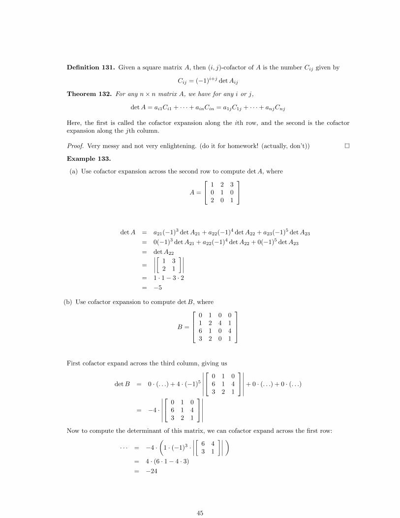
Definition 131. Given a square matrix A, then (i, j)-cofactor of A is the number Cij given by

Cij = (−1)i+j detAij

Theorem 132. For any n× n matrix A, we have for any i or j,

detA = ai1Ci1 + · · ·+ ainCin = a1jC1j + · · ·+ anjCnj

Here, the first is called the cofactor expansion along the ith row, and the second is the cofactorexpansion along the jth column.

Proof. Very messy and not very enlightening. (do it for homework! (actually, don’t))

Example 133.

(a) Use cofactor expansion across the second row to compute detA, where

A =

1 2 30 1 02 0 1

detA = a21(−1)3 detA21 + a22(−1)4 detA22 + a23(−1)5 detA23

= 0(−1)3 detA21 + a22(−1)4 detA22 + 0(−1)5 detA23

= detA22

=

∣∣∣∣[ 1 32 1

]∣∣∣∣= 1 · 1− 3 · 2= −5

(b) Use cofactor expansion to compute detB, where

B =

0 1 0 01 2 4 16 1 0 43 2 0 1

First cofactor expand across the third column, giving us

detB = 0 · (. . .) + 4 · (−1)5

∣∣∣∣∣∣ 0 1 0

6 1 43 2 1

∣∣∣∣∣∣+ 0 · (. . .) + 0 · (. . .)

= −4 ·

∣∣∣∣∣∣ 0 1 0

6 1 43 2 1

∣∣∣∣∣∣Now to compute the determinant of this matrix, we can cofactor expand across the first row:

· · · = −4 ·(

1 · (−1)3 ·∣∣∣∣[ 6 4

3 1

]∣∣∣∣ )= 4 · (6 · 1− 4 · 3)

= −24

45

(c) Use cofactor expansion to compute the determinant of the following matrix

C =

a b c d0 e f g0 0 h i0 0 0 j

First cofactor-expand along the first column:

detC = a

∣∣∣∣∣∣ e f g

0 h i0 0 j

∣∣∣∣∣∣then again expand along the first column of the 3× 3 matrix:

· · · = a ·(e

∣∣∣∣[ h i0 j

]∣∣∣∣ )and then again...

· · · = a · (e(hj)) = aehj

Indeed, this illustrates the following fact:

Definition 134. A triangular matrix is a square matrix such that all entries either above or belowthe main diagonal are zero.

In the case where everything below the diagonal are zeros, we call the matrix upper triangular. Ifeverything above the diagonal are zero, we call it lower triangular.

Theorem 135. If A is a triangular matrix, then detA is the product of all the entries on the maindiagonal.

Proof. We’ve already seen that if A is upper-triangular, repeated cofactor expansion along the firstcolumn proves the claim. For the case where A is lower-triangular, simply cofactor-expand acrossthe first row.

Corollary 136. If A is a triangular matrix with a zero on the main diagonal, then detA = 0.

Properties of Determinants

Now that we know how to compute determinants, what are they good for?

Before proceeding, we’ll take this theorem for granted:

Theorem 137. If A,B are square matrices of the same size, then |AB| = |A||B|.

Proof. Kind of difficult. Assuming this however makes proving other stuff a lot simpler.

Theorem 138. |A| = |AT |.

Proof. This comes from the fact that you can either cofactor-expand along rows or columns, withoutchanging the value of the determinant. Proving this is also unnecessarily messy and unenlightening.

46

Example 139. Compute the determinant of the following matrices:

E1 =

k 0 00 1 00 0 1

E2 =

0 1 01 0 00 0 1

E3 =

1 0 00 1 k0 0 1

The first and third are triangular, and it’s easily seen that |E1| = k and |E3| = 1.

On the other hand, cofactor-expanding along either the third row or column will show that |E2| = −1.

In fact, this illustrates a more general fact, which we also won’t prove in full rigor:

Theorem 140. Let E be an elementary matrix, and let I be the identity matrix of the same size.

(a) If E was obtained by scaling a row of I by k, then |E| = k.

(b) If E was obtained by interchanging two rows of I, then |E| = −1.

(c) If E was obtained by a row replacement operation, then |E| = 1.

In particular, the determinant of any elementary matrix is always nonzero.

Corollary 141. Let A be a square matrix.

(a) If B is obtained by scaling a row of A by k, then |B| = k|A|.(b) If B is obtained by interchanging two rows of A, then |B| = −|A|.(c) If B is obtained by applying a row-replacement operation to A, then |B| = |A|.

Proof. This corollary just comes from the fact that applying an elementary row operation corre-sponds to multiplying by the appropriate elementary matrix. Ie, in (a), B = EA, where E is theelementary matrix representing the “scale a row k” operation, so applying the multiplicativity ofthe determinant, we have

|B| = |EA| = |E||A| = k|A|

The same technique also proves (b) and (c).

IN FACT! Since |A| = |AT |, the previous corollary is true when “row” is replaced by “column”.

Example 142. Now suppose A is row-equivalent to the matrix

B =

1 2 30 −1 20 0 0

What is detA?

First note that |B| = 0 (it’s triangular with a 0 on the main diagonal).

Now, to say that A ∼ B is to say that there exist elementary matrices E1, . . . , En such that

B = EnEn−1 · · ·E1A so |B|︸︷︷︸0

= |EnEn−1 · · ·E1A| = |En||En−1| · · · |E1||A|

But since none of the Ei’s have determinant zero, so since |B| = 0, we must also have |A| = 0.

Warning. Note that in general, if B ∼ A, it is NOT true that |B| = |A|. However, we do knowthat if one of them is zero, then the other is zero, since multiplying by elementary matrices cannotmake nonzero determinants zero.

This example demonstrates the following fact:

47

Corollary 143. Suppose A,B are square matrices and A ∼ B, then |A| = 0 if and only if |B| = 0.

Example 144. Suppose A is a square matrix. Let B be any echelon form of A.

(a) Is B triangular?

Yes, in fact it’s upper-triangular.

(b) If A is invertible, what can you tell about detB?

Since it’s invertible, it must have a pivot in every row/column. Since B is in echelon form,every diagonal entry must be a row-leader, and hence is nonzero. Thus, detB 6= 0.

(b) If A is not invertible, what can you say about detB?

If A is not invertible, then it won’t have a pivot in every row/column. Just thinking about thepossible echelon forms of a square matrix that don’t have a pivot in every row/column, we seethat at least one of the diagonal entries must be zero, hence detB = 0.

Combined with the previous corollary, we get the following theorem:

Theorem 145. A square matrix A is invertible if and only if detA 6= 0.

Notation. For any n×n matrix A and b ∈ Rn, let Ai(b) be the matrix obtained from A by replacingcolumn i by the vector b.

Theorem 146. Let A be an invertible n × n matrix. For any b ∈ Rn, the unique solution x ofAx = b has entries given by

xi =detAi(b)

detAi = 1, 2, . . . , n

48

17. Lecture 17. Eigenvectors/Eigenvalues/Eigenspaces. Sections 5.1 and 5.2. Pset 6 due thursday.

Example 147. Consider the matrix

A =

[4 −12 1

], we can compute: A

[10

]=

[42

]A

[01

]=

[−1

1

]So at first the action of A on the plane is difficult to describe. On the other hand, we can ask:

Does there exist a vector x ∈ R2 such that Ax = λx for some λ ∈ R? (in other words, do there existvectors x ∈ R2 that are scaled by A?

Definition 148. An eigenvector of a square matrix A is a nonzero vector x such that Ax = λxfor some λ ∈ R. An eigenvalue of a matrix A is a number λ such that for some nonzero vector x,Ax = λx.

Here, λ is the eigenvalue corresponding to the eigenvector x, and x is an eigenvector w eigenvalue λ.

Example 149. Let A =

[4 −12 1

]as above.

(a) Is

[21

]an eigenvector of A?

We can compute

[4 −12 1

] [21

]=

[75

]6= λ

[21

]for any λ ∈ R, and hence is not an

eigenvector.

(b) Is

[12

]an eigenvector of A?

We can compute

[4 −12 1

] [12

]=

[24

]= 2

[12

], so

[12

]is an eigenvector of A with

eigenvalue λ = 2.

Thus, we see that indeed there do exist vectors x ∈ R2 that are scaled by A. Now that we haveone, we can ask

(c) How many eigenvectors of A are there?

Infinitely many! This is because if Ax = λx, then for any c ∈ R, A(cx) = c(Ax) = cλx = λ(cx),so cx is also an eigenvector (as long as c 6= 0).

In fact, note that if x, y are eigenvectors of A with eigenvalue λ, then Ax = λx and Ay = λy,so

A(x+ y) = Ax+Ay = λx+ λy = λ(x+ y),

which shows that (x+ y) is also an eigenvector of A with the same eigenvalue!

(d) Let λ ∈ R, then is the set of all eigenvectors of A with eigenvalue λ a subspace of R2?

Almost! (but not quite). Note that technically, the zero vector ~0 is not an eigenvector. However,the above computations show that

The set of all eigenvectors of A with eigenvalue λ, together with ~0, is a subspace of R2

We’ll see this in another light later on.

Now, we’ve found that A has infinitely many eigenvectors. However, all the examples we’ve got areall scalar multiples of (1, 2), so now we may ask : are these the only eigenvectors of A? To answerthis question, we’ll first consider another:

49

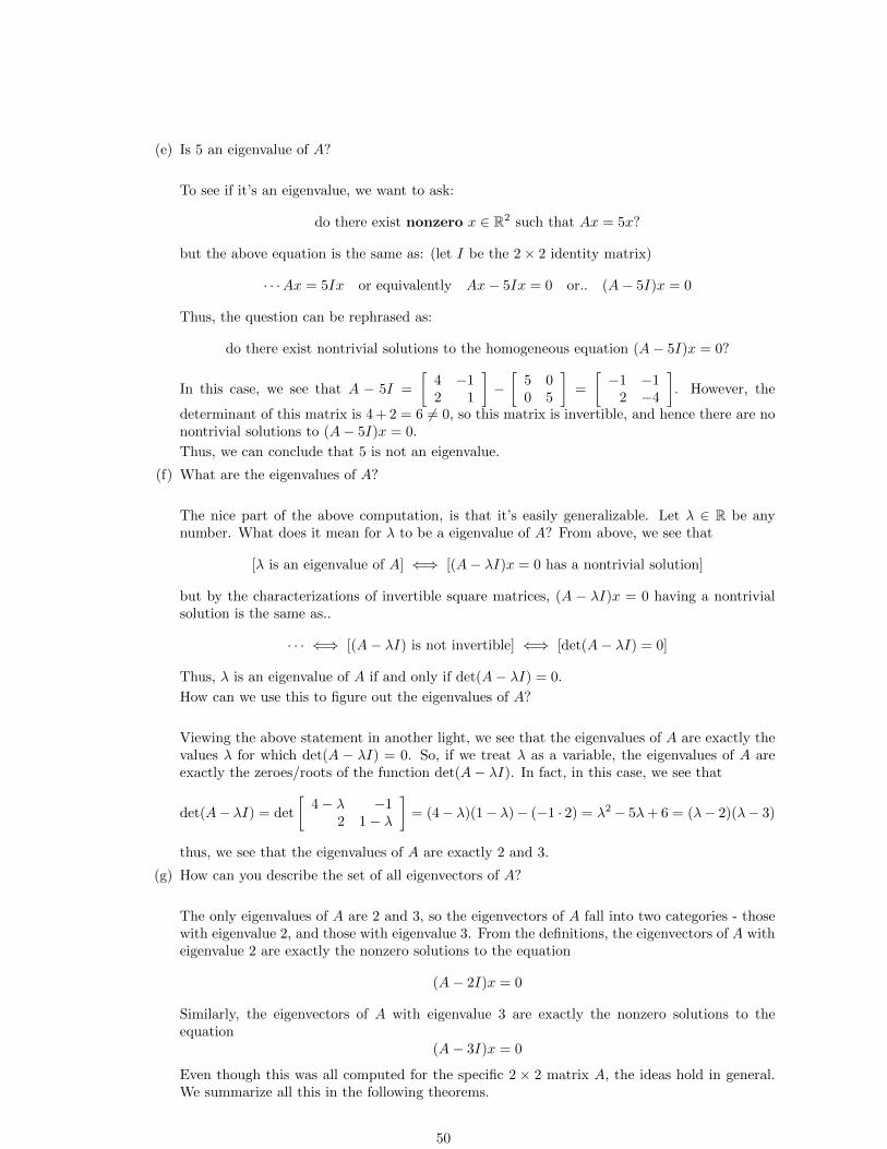
(e) Is 5 an eigenvalue of A?

To see if it’s an eigenvalue, we want to ask:

do there exist nonzero x ∈ R2 such that Ax = 5x?

but the above equation is the same as: (let I be the 2× 2 identity matrix)

· · ·Ax = 5Ix or equivalently Ax− 5Ix = 0 or.. (A− 5I)x = 0

Thus, the question can be rephrased as:

do there exist nontrivial solutions to the homogeneous equation (A− 5I)x = 0?

In this case, we see that A − 5I =

[4 −12 1

]−[

5 00 5

]=

[−1 −1

2 −4

]. However, the

determinant of this matrix is 4 + 2 = 6 6= 0, so this matrix is invertible, and hence there are nonontrivial solutions to (A− 5I)x = 0.

Thus, we can conclude that 5 is not an eigenvalue.

(f) What are the eigenvalues of A?

The nice part of the above computation, is that it’s easily generalizable. Let λ ∈ R be anynumber. What does it mean for λ to be a eigenvalue of A? From above, we see that

[λ is an eigenvalue of A] ⇐⇒ [(A− λI)x = 0 has a nontrivial solution]

but by the characterizations of invertible square matrices, (A − λI)x = 0 having a nontrivialsolution is the same as..

· · · ⇐⇒ [(A− λI) is not invertible] ⇐⇒ [det(A− λI) = 0]

Thus, λ is an eigenvalue of A if and only if det(A− λI) = 0.

How can we use this to figure out the eigenvalues of A?

Viewing the above statement in another light, we see that the eigenvalues of A are exactly thevalues λ for which det(A − λI) = 0. So, if we treat λ as a variable, the eigenvalues of A areexactly the zeroes/roots of the function det(A− λI). In fact, in this case, we see that

det(A− λI) = det

[4− λ −1

2 1− λ

]= (4− λ)(1− λ)− (−1 · 2) = λ2 − 5λ+ 6 = (λ− 2)(λ− 3)

thus, we see that the eigenvalues of A are exactly 2 and 3.

(g) How can you describe the set of all eigenvectors of A?

The only eigenvalues of A are 2 and 3, so the eigenvectors of A fall into two categories - thosewith eigenvalue 2, and those with eigenvalue 3. From the definitions, the eigenvectors of A witheigenvalue 2 are exactly the nonzero solutions to the equation

(A− 2I)x = 0

Similarly, the eigenvectors of A with eigenvalue 3 are exactly the nonzero solutions to theequation

(A− 3I)x = 0

Even though this was all computed for the specific 2 × 2 matrix A, the ideas hold in general.We summarize all this in the following theorems.

50

Theorem 150. A number λ is an eigenvalue for a square matrix A if and only if there is a nontrivialsolution to the equation

(A− λI)x = 0

Definition 151. Let A be an n× n square matrix, then det(A− λI) as a function in the variableλ is a polynomial of degree n. We call this the characteristic polynomial of A, denoted

χA(λ) = det(A− λI)

Corollary 152. The eigenvalues of any square matrix A are the roots of the polynomial χA(λ).

Definition 153. For any square matrix A and λ ∈ R, the eigenspace of A corresponding to λ (orthe λ-eigenspace) is the solution set of the equation

(A− λI)x = 0

Note that λ is an eigenvalue iff its eigenspace is nontrivial (ie, has dimension > 0)

Note. Here, we’re certainly justified in using the name “eigenspace” in the above definition. Indeed,if x ∈ Rn is an eigenvector of an n×n matrix A with eigenvalue λ, then Ax = λx, so (A−λI)x = 0, sox is indeed in the λ-eigenspace of A. Thus, the λ-eigenspace of A certainly contains all eigenvectorsof A with eigenvalue λ.

Furthermore, everything (except ~0) in the λ-eigenspace is also an eigenvector, since

(A− λI)x = 0 is to say Ax = λx

Thus, we see that the λ-eigenspace is exactly the set of all eigenvectors of A with eigenvalue λ,together with the vector ~0.

Corollary 154. An n× n matrix A is invertible if and only if 0 is not an eigenvalue for A.

Proof. If it’s noninvertible, then there must be a nonzero vector x ∈ Rn such that Ax = 0, but that’sto say that 0 is an eigenvalue of A.

Conversely, if A is invertible, then (A−0I)x = Ax = 0 has no nontrivial solutions, so the 0-eigenspaceis trivial, so 0 is not an eigenvalue of A.

Example 155. Let A =

4 −1 62 1 62 −1 8

. Find a basis for the 2-eigenspace.

By definition, the 2-eigenspace is exactly the null space of the matrix

A− 2I =

2 −1 62 −1 62 −1 6

∼ 2 −1 6

0 0 00 0 0

Since this matrix has two non-pivot columns, the equation (A − 2I)x = 0 has a null space ofdimension 2. To find a basis for the null space, simply find the parametric form of the solution setof (A− 2I)x = 0 and apply theorem 111.

Example 156. Now consider the matrix

A =

1 2 −40 2 20 0 −5

What are the eigenvalues of this matrix?

51

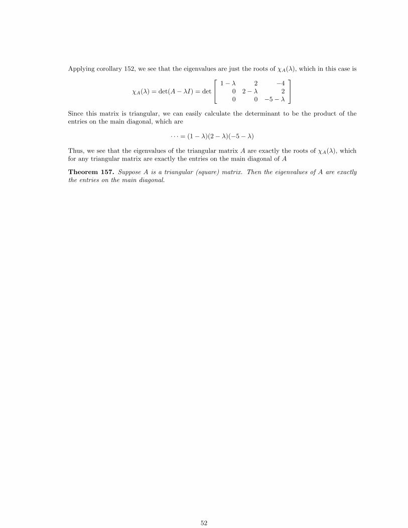
Applying corollary 152, we see that the eigenvalues are just the roots of χA(λ), which in this case is

χA(λ) = det(A− λI) = det

1− λ 2 −40 2− λ 20 0 −5− λ

Since this matrix is triangular, we can easily calculate the determinant to be the product of theentries on the main diagonal, which are

· · · = (1− λ)(2− λ)(−5− λ)

Thus, we see that the eigenvalues of the triangular matrix A are exactly the roots of χA(λ), whichfor any triangular matrix are exactly the entries on the main diagonal of A

Theorem 157. Suppose A is a triangular (square) matrix. Then the eigenvalues of A are exactlythe entries on the main diagonal.

52

18. Lecture 18. Sections 5.1 and 5.2, Problem Set 6 due NOW! Problem set 7 due next next tuesday.

Firstly, recall the theorem that described how applying row operations to your matrix affects thedeterminant (thm 141). To summarize, the theorem said:

– scaling a row by k also scales the determinant by k.

– interchanging two rows flips the sign of the determinant.

– applying a replacement operation does not change the determinant.

Now, even though A ∼ B doesn’t mean |A| = |B|, in some situations we can profitably use theabove theorem to compute the determinant of various matrices.

Example 158. Compute the determinant of the following matrices:

(a) A =

0 4 51 2 30 0 6

There are a number of ways. Using cofactor expansion, you can either expand along the bottomrow, or the leftmost column. If you expand along the bottom row, you get

|A| = 6 ·∣∣∣∣[ 0 4

1 2

]∣∣∣∣ = 6 · (−4 · 1) = −24

If you cofactor expand along the leftmost column, you get:

|A| = 1 ·∣∣∣∣[ 4 5

0 6

]∣∣∣∣ = −1 · 4 · 6 = −24

Or, you could note that swapping the first two rows gives you a triangular matrix, whose diag-onal entries are 1, 4, 6, so the triangular matrix you get after the interchange has determinant24, so the original matrix has determinant -24.

(b) B =

1 2 31 2 40 3 −1

This matrix is a little lacking in zeroes, so cofactor expansion will be a little difficult. However,note that if you subtract the first row from the second and then interchange the last two rows,we get:

· · · ∼

1 2 30 0 10 3 −1

∼ 1 2 3

0 3 −10 0 1

which has determinant 3. Since we applied only a row replacement and an interchange operationto get to this triangular matrix, the original matrix B must have had determinant -3.

Alright, back to eigenvectors. Last time, we learned how to find the eigenvectors of any matrix.

Example 159.

(a) What are the eigenvalues of the matrix

A =

−1 4 80 3 00 0 3

Recall that for any matrix A, the eigenvalues of the matrix are exactly the roots of the poly-nomial det(A− λI). In this case, this polynomial is:

χA(λ) =

∣∣∣∣∣∣ −1− λ 4 8

0 3− λ 00 0 3− λ

∣∣∣∣∣∣ = (−1−λ)(3−λ)(3−λ) (since this matrix is triangular)

53

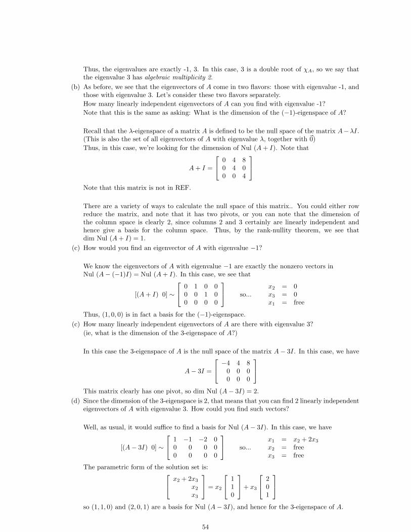
Thus, the eigenvalues are exactly -1, 3. In this case, 3 is a double root of χA, so we say thatthe eigenvalue 3 has algebraic multiplicity 2.

(b) As before, we see that the eigenvectors of A come in two flavors: those with eigenvalue -1, andthose with eigenvalue 3. Let’s consider these two flavors separately.

How many linearly independent eigenvectors of A can you find with eigenvalue -1?

Note that this is the same as asking: What is the dimension of the (−1)-eigenspace of A?

Recall that the λ-eigenspace of a matrix A is defined to be the null space of the matrix A−λI.(This is also the set of all eigenvectors of A with eigenvalue λ, together with ~0)

Thus, in this case, we’re looking for the dimension of Nul (A+ I). Note that

A+ I =

0 4 80 4 00 0 4

Note that this matrix is not in REF.

There are a variety of ways to calculate the null space of this matrix.. You could either rowreduce the matrix, and note that it has two pivots, or you can note that the dimension ofthe column space is clearly 2, since columns 2 and 3 certainly are linearly independent andhence give a basis for the column space. Thus, by the rank-nullity theorem, we see thatdim Nul (A+ I) = 1.

(c) How would you find an eigenvector of A with eigenvalue −1?

We know the eigenvectors of A with eigenvalue −1 are exactly the nonzero vectors inNul (A− (−1)I) = Nul (A+ I). In this case, we see that

[(A+ I) 0] ∼

0 1 0 00 0 1 00 0 0 0

so...x2 = 0x3 = 0x1 = free

Thus, (1, 0, 0) is in fact a basis for the (−1)-eigenspace.

(c) How many linearly independent eigenvectors of A are there with eigenvalue 3?

(ie, what is the dimension of the 3-eigenspace of A?)

In this case the 3-eigenspace of A is the null space of the matrix A− 3I. In this case, we have

A− 3I =

−4 4 80 0 00 0 0

This matrix clearly has one pivot, so dim Nul (A− 3I) = 2.

(d) Since the dimension of the 3-eigenspace is 2, that means that you can find 2 linearly independenteigenvectors of A with eigenvalue 3. How could you find such vectors?

Well, as usual, it would suffice to find a basis for Nul (A− 3I). In this case, we have

[(A− 3I) 0] ∼

1 −1 −2 00 0 0 00 0 0 0

so...x1 = x2 + 2x3x2 = freex3 = free

The parametric form of the solution set is: x2 + 2x3x2x3

= x2

110

+ x3

201

so (1, 1, 0) and (2, 0, 1) are a basis for Nul (A− 3I), and hence for the 3-eigenspace of A.

54

To summarize, given a matrix A, we’ve found bases for both the (-1)-eigenspace and the 3-eigenspaceof A:

basis for the (-1)-eigenspace :

1

00

basis for the 3-eigenspace:

1

10

, 2

01

Note in particular that if we put these vectors together, the set:

100

, 1

10

, 2

01

form a basis for R3 (why is this?)

Thus, in the case of A, we’ve found a basis for R3 consisting of eigenvectors. Geometrically, thismeans that we can describe the effect that A has on R3 in terms of vectors that are scaled by A.This gives us a nice way of understanding how the matrix A acts on R3.

In fact... let v = (1, 1, 0). Note that v is an eigenvector of A with eigenvalue 3. Then, lets computeA2v:

A2v = A(Av) = A(3v) = 3Av = 3(3v) = 9v

A good way to think about it is as follows: If x is an eigenvector for a 3 × 3 matrix B, then youwant to think of Span {x} as being a “track” in 3-space such that applying B to any vector on thissubspace just pushes the vector further along, and the speed at which the vector is pushed alongthe track is just the eigenvalue. In the case of the matrix A above, it has three linearly independenttracks, one with “speed” -1, and two with “speed” 3.

In the case of the above computation, we saw that applying A two times to v essentially just pushedit along the v-track with speed 3, two times (of course, speed is probably not the right word here,since we ended up with A2v = 9v (as opposed to 6v), but it’s okay as an analogy).

In general, n× n matrices B for which it is possible to find a basis of Rn consisting of eigenvectorsof B are called diagonalizable. We’ll see why this is in a moment, but first, some setup:

Definition 160. Two matrices A,B are similar if there exists an invertible matrix P such thatA = PBP−1.

Lemma 161. If P is an invertible matrix, then |P−1| = 1/|P |.

Proof. Note that I = PP−1, so 1 = |I| = |PP−1| = |P ||P−1|, so |P−1| = 1/|P |.

Theorem 162. If two matrices A,B are similar, then χA = χB.

Proof. Suppose A,B are similar, ie, A = PBP−1 for some invertible matrix P , then

A− λI = PBP−1 − λPIP−1 = P (B − λI)P−1

taking determinants, we get:

χA = |A− λI| = |P (B − λI)P−1| = |P ||B − λI||P−1| = |B − λI| = χB

Definition 163. A diagonal matrix is a square matrix that is both upper and lower triangular. (ie,the only nonzero entries are on the main diagonal)

Example 164. Let D =

−1 0 00 3 00 0 3

. Clearly D is diagonal.

55

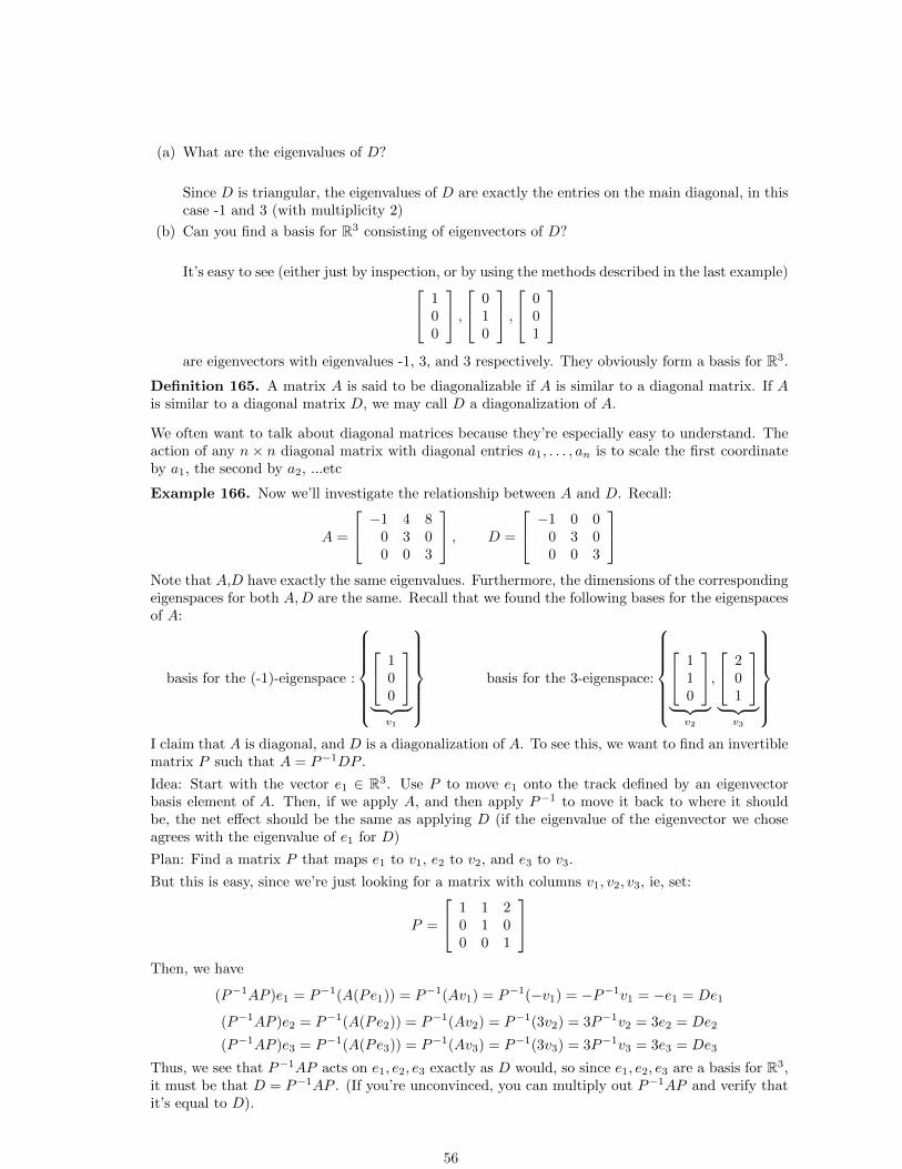
(a) What are the eigenvalues of D?

Since D is triangular, the eigenvalues of D are exactly the entries on the main diagonal, in thiscase -1 and 3 (with multiplicity 2)

(b) Can you find a basis for R3 consisting of eigenvectors of D?

It’s easy to see (either just by inspection, or by using the methods described in the last example) 100

, 0

10

, 0

01

are eigenvectors with eigenvalues -1, 3, and 3 respectively. They obviously form a basis for R3.

Definition 165. A matrix A is said to be diagonalizable if A is similar to a diagonal matrix. If Ais similar to a diagonal matrix D, we may call D a diagonalization of A.

We often want to talk about diagonal matrices because they’re especially easy to understand. Theaction of any n× n diagonal matrix with diagonal entries a1, . . . , an is to scale the first coordinateby a1, the second by a2, ...etc

Example 166. Now we’ll investigate the relationship between A and D. Recall:

A =

−1 4 80 3 00 0 3

, D =

−1 0 00 3 00 0 3

Note that A,D have exactly the same eigenvalues. Furthermore, the dimensions of the correspondingeigenspaces for both A,D are the same. Recall that we found the following bases for the eigenspacesof A:

basis for the (-1)-eigenspace :

1

00

︸︷︷︸

v1

basis for the 3-eigenspace:

1

10

︸︷︷︸

v2

,

201

︸︷︷︸

v3

I claim that A is diagonal, and D is a diagonalization of A. To see this, we want to find an invertiblematrix P such that A = P−1DP .

Idea: Start with the vector e1 ∈ R3. Use P to move e1 onto the track defined by an eigenvectorbasis element of A. Then, if we apply A, and then apply P−1 to move it back to where it shouldbe, the net effect should be the same as applying D (if the eigenvalue of the eigenvector we choseagrees with the eigenvalue of e1 for D)

Plan: Find a matrix P that maps e1 to v1, e2 to v2, and e3 to v3.

But this is easy, since we’re just looking for a matrix with columns v1, v2, v3, ie, set:

P =

1 1 20 1 00 0 1

Then, we have

(P−1AP )e1 = P−1(A(Pe1)) = P−1(Av1) = P−1(−v1) = −P−1v1 = −e1 = De1

(P−1AP )e2 = P−1(A(Pe2)) = P−1(Av2) = P−1(3v2) = 3P−1v2 = 3e2 = De2

(P−1AP )e3 = P−1(A(Pe3)) = P−1(Av3) = P−1(3v3) = 3P−1v3 = 3e3 = De3

Thus, we see that P−1AP acts on e1, e2, e3 exactly as D would, so since e1, e2, e3 are a basis for R3,it must be that D = P−1AP . (If you’re unconvinced, you can multiply out P−1AP and verify thatit’s equal to D).

56

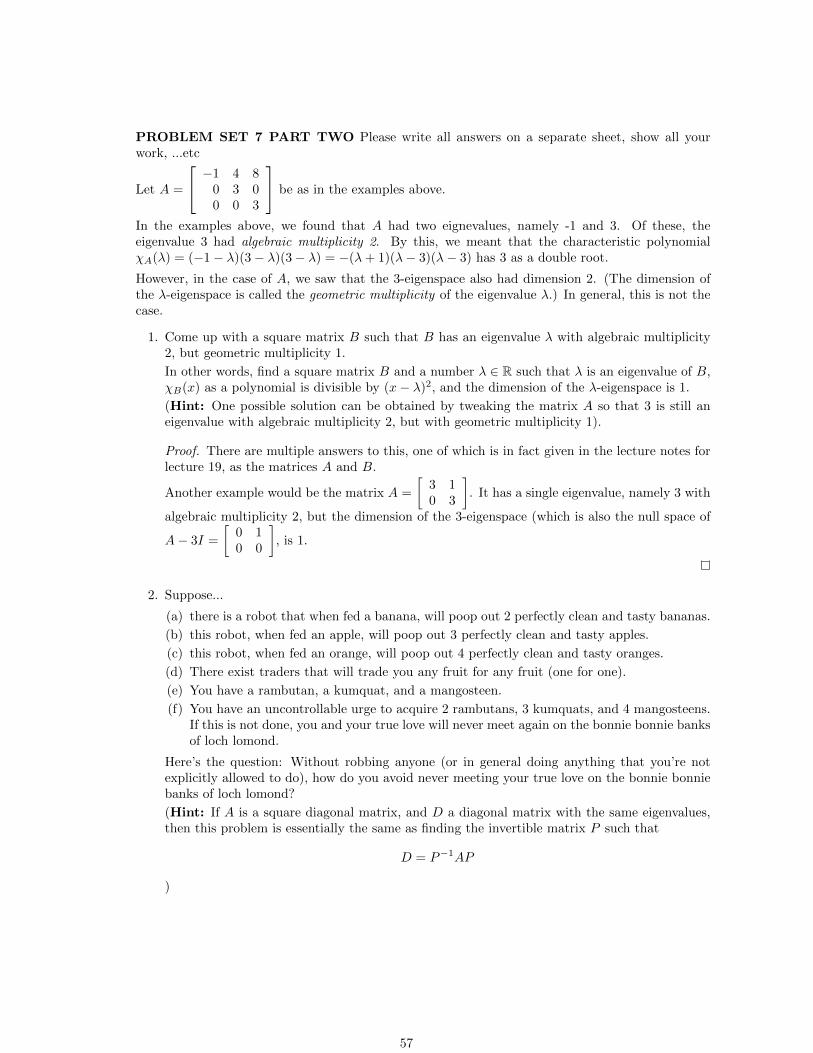
PROBLEM SET 7 PART TWO Please write all answers on a separate sheet, show all yourwork, ...etc

Let A =

−1 4 80 3 00 0 3

be as in the examples above.

In the examples above, we found that A had two eignevalues, namely -1 and 3. Of these, theeigenvalue 3 had algebraic multiplicity 2. By this, we meant that the characteristic polynomialχA(λ) = (−1− λ)(3− λ)(3− λ) = −(λ+ 1)(λ− 3)(λ− 3) has 3 as a double root.

However, in the case of A, we saw that the 3-eigenspace also had dimension 2. (The dimension ofthe λ-eigenspace is called the geometric multiplicity of the eigenvalue λ.) In general, this is not thecase.

1. Come up with a square matrix B such that B has an eigenvalue λ with algebraic multiplicity2, but geometric multiplicity 1.

In other words, find a square matrix B and a number λ ∈ R such that λ is an eigenvalue of B,χB(x) as a polynomial is divisible by (x− λ)2, and the dimension of the λ-eigenspace is 1.

(Hint: One possible solution can be obtained by tweaking the matrix A so that 3 is still aneigenvalue with algebraic multiplicity 2, but with geometric multiplicity 1).

Proof. There are multiple answers to this, one of which is in fact given in the lecture notes forlecture 19, as the matrices A and B.

Another example would be the matrix A =

[3 10 3

]. It has a single eigenvalue, namely 3 with

algebraic multiplicity 2, but the dimension of the 3-eigenspace (which is also the null space of

A− 3I =

[0 10 0

], is 1.

2. Suppose...

(a) there is a robot that when fed a banana, will poop out 2 perfectly clean and tasty bananas.

(b) this robot, when fed an apple, will poop out 3 perfectly clean and tasty apples.

(c) this robot, when fed an orange, will poop out 4 perfectly clean and tasty oranges.

(d) There exist traders that will trade you any fruit for any fruit (one for one).

(e) You have a rambutan, a kumquat, and a mangosteen.

(f) You have an uncontrollable urge to acquire 2 rambutans, 3 kumquats, and 4 mangosteens.If this is not done, you and your true love will never meet again on the bonnie bonnie banksof loch lomond.

Here’s the question: Without robbing anyone (or in general doing anything that you’re notexplicitly allowed to do), how do you avoid never meeting your true love on the bonnie bonniebanks of loch lomond?

(Hint: If A is a square diagonal matrix, and D a diagonal matrix with the same eigenvalues,then this problem is essentially the same as finding the invertible matrix P such that

D = P−1AP

)

57

19. Lecture 19. Homework 7 online. Yes, it’s all extra credit! (whatever that means)

Notation. From now on, the act of “diagonalizing a matrix A” will refer to the process of findinga diagonal matrix D such that A = PDP−1 for some invertible matrix P . (Note this is equivalentto finding D,P such that D = PAP−1, or D = P−1AP , or A = P−1DP ).

Last time we saw how to diagonalize the matrix A =

−1 4 80 3 00 0 3

.

Now, lets try to diagonalize another matrix.

Example 167. Consider the matrix B =

−1 4 80 3 10 0 3

.

(a) What are the eigenvalues of B?

Recall that the eigenvalues of a matrix B are exactly the roots of its characteristic polynomial.In this case, we have

χB(λ) =

∣∣∣∣∣∣ −1− λ 4 8

0 3− λ 10 0 3− λ

∣∣∣∣∣∣ = (−1− λ)(3− λ)(3− λ)

Thus, the eigenvalues are again −1 and 3, with the eigenvalue 3 having algebraic multiplicity 2.

(b) Find a basis for the −1-eigenspace of B.

Again, the −1-eigenspace of B is just the solution set of (B − (−I))x = (B + I)x = 0. In thiscase, we have

B + I =

0 4 80 4 10 0 4

So, we get:

[(B + I) 0] ∼

0 1 0 00 0 1 00 0 0 0

x1 = freex2 = 0x3 = 0

so parametric solution is: x1

100

And hence (1, 0, 0) is a basis for the −1-eigenspace, just as in the case with A.

(c) Find a basis for the 3-eigenspace of B.

As usual, this is the same as finding a basis for Nul (B − 3I). In this case, we have

B − 3I =

−4 4 80 0 10 0 0

so...

[(B − 3I) 0] ∼

1 −1 0 00 0 1 00 0 0 0

so...x1 = x2x2 = freex3 = 0

The parametric form of the solution set is: x2x20

= x2

110

so (1, 1, 0) is a basis for the 3-eigenspace of B. This is the crucial difference between A and B. Whilethe 3-eigenspace of A has dimension 2, the 3-eigenspace of B has dimension 1.

58

(d) Is B diagonalizable?

What happens when you try to diagonalize it? Well, your best guess for a diagonalization of Bwould probably be something like

D =

−1 0 00 3 00 0 3

just like the diagonalization of A. Now, we have to find a suitable invertible matrix P such thatD = P−1BP . Let’s try our old idea, ie

(a) We want the process of first multiplying by P , then B, then P−1 to be the same as the effect ofmultiplying by D. To show this, it suffices to show that P−1BPe1 = De1, and similarly withe2, e3.

(b) To do this, we’ll want to let B do most of the work, and use P to trade the input vectorse1, e2, e3 into vectors we can use B to scale. Thus, we’ll want to map e1, e2, e3 to eigenvectorsof B.

But at this point, we see we’re stuck! Why? Well, first, lets consider the following lemma:

Lemma 168. Let T : Rn → Rn be a linear transformation. Let {v1, . . . , vp} ⊆ Rn be linearlyindependent. Suppose now that {T (v1), . . . , T (vp)} is linearly dependent. Then T isn’t invertible!

Proof. Firstly, note that since {T (v1), . . . , T (vp)} is linearly dependent, the dimension of their span isstrictly lower than p. Now, what’s essentially happening here is that T is mapping vectors that spana p-dimensional subspace, and squeezing them into a subspace of lower dimension. In other words,you can think of T as mapping a big space to a small space, so naturally T discards information,and hence can’t be invertible!

More formally, suppose a1T (v1) + · · · + apT (vp) = 0 is a nontrivial linear dependence relation (ie,not all the ai’s are 0). On the other hand, we have (by linearity of T ):

0 = a1T (v1) + · · ·+ apT (vp) = T (a1v1 + · · · apvp)

Since the ai’s are not all 0, and v1, . . . , vp are linearly independent, this means that a1v1+· · · apvp 6= 0,so T maps a nonzero vector to 0, so since it also maps 0 to 0, it’s not 1-1, and hence not invertible.

Now let’s return to the question of finding a suitable invertible matrix P such that D = P−1BP .Now, via the lemma, we see that for P to be invertible, we must define P by sending e1, e2, e3 tolinearly independent eigenvectors of B. Why is this impossible?

It’s impossible because the eigenvectors of D all come in two flavors, either with eigenvalue -1 orwith eigenvalue 3. However, since the (-1)-eigenspace has dimension 1, and the 3-eigenspace hasdimension 1, we see that we can find at most two linearly independent eigenvectors of B!

Thus, this shows that our method, given our initial guess for D, is doomed to failure! As it turnsout, for this particular matrix B, there does not exist a diagonal matrix that is similar to B. Ie, Bis not diagonalizable! In fact, we have a more general theorem:

59

Theorem 169. An n × n matrix A is diagonalizable if and only if A has n linearly independenteigenvectors.

Proof. First we’ll show that if A is diagonalizable, then it must have n linearly independent eigen-vectors. To see this, suppose A = PDP−1 for some invertible matrix P and diagonal matrix D.Suppose

D =

d1 0 00 d2 00 0 d3

Then, what are the vectors that P−1 maps to e1, e2, e3?

Well, clearly P ~e1, P ~e2, P ~e3 are the columns of P , so if P = [~p1 ~p2 ~p3], then P−1 must map ~p1, ~p2, ~p3to ~e1, ~e2, ~e3 respectively (since inverses reverse the action of the original map).

Now, note that for i = 1, 2, 3, we have:

A~pi = PDP−1~pi = PD~ei = P (di~ei) = di(P ~ei) = di~pi

Thus we see that p1, p2, p3 are eigenvectors of A with eigenvalues d1, d2, d3. On the other hand,we know that since ~p1, ~p2, ~p3 are the columns of P , and P is invertible, they must be linearlyindependent, so indeed we’ve found 3 linearly independent eigenvectors of A!

Now suppose that v1, v2, v3 are three linearly independent eigenvectors of A (with eigenvaluesλ1, λ2, λ3. Then, we want to find an invertible matrix P such that D = P−1AP for some diag-onal matrix D. As described earlier, we’d like P to map e1, e2, e3 to v1, v2, v3. Thus, if you letP = [v1 v2 v3], we’d have that for i = 1, 2, 3

P−1APei = P−1Avi = P−1λivi = λi(P−1vi) = λiei

But this tells you exactly that the columns of P−1AP are λ1e1, λ2e2, and λ3e3. In other words,

P−1AP = [λ1e1 λ2e2 λ3e3]

which is indeed diagonal!

Important! Note that here, all we needed was for P to map the set {e1, e2, e3} onto the set{v1, v2, v3}. It didn’t necessarily need to map ei to vi. Ie, it could mix them up a bit. For example,if P = [v2 v3 v1], this would still work! (Though you’d end up with another diagonal matrix D)

In fact, I would urge you to try this on the homework. Ie, when diagonalizing, try mixing up theorder a bit and see what happens.

Example 170. Consider the matrix A =

1 2 30 2 30 0 3

. Is it diagonalizable?

So, by the above theorem 169, we see that A is diagonalizable if and only if it has 3 linearlyindependent eigenvectors. To see this, we’ll first ask, what are the eigenvalues of A?

As usual, since A is triangular, the eigenvalues are just the entries down the main diagonal. Inthis case, 1, 2, and 3. Thus, this shows that the eigenvectors of A come in 3 flavors - those witheigenvalue 1, those with eigenvalue 2, and those with eigenvalue 3. Thus, each of those eigenvalueswill come with its own eigenspace, each of which in this case will be 1-dimensional. Let v1, v2, v3 beeigenvectors corresponding to the eigenvalues 1, 2, 3. Are these eigenvectors linearly independent?In fact, they are:

60

Theorem 171. If A is an n× n matrix with eigenvectors v1, . . . , vp with eigenvalues λ1, . . . , λp. Ifthe eigenvalues are all distinct, then {v1, . . . , vp} are linearly independent.

Proof. Suppose {v1, . . . , vp} were linearly dependent, then we a1, . . . , ap, not all zero, such thata1v1 + · · · + apvp = 0. Now, there may be many choices for the ai’s, so choose the ai’s so that asmany ai’s are zero as possible. Ie, find a linear dependence relation that involves as few vectors aspossible. Possibly reordering/renaming the vectors, suppose the vectors involved in this minimalrelation are v1, . . . , vr, so we have:

a1v1 + · · ·+ arvr = 0

where a1, . . . , ar are all nonzero, and there is no smaller nontrivial linear combination of v1, . . . , vrthat equals 0. Now, if we apply T , we get:

T (a1v1 + · · ·+ arvr) = a1T (v1) + · · · arT (vr) = a1λ1v1 + · · ·+ arλrvr = 0

On the other hand, multiplying the entire relation by λr, we get

a1λrv1 + a2λrv1 + · · ·+ arλrvr = 0

Thus, subtracting the two equations, we get:

a1(λ1 − λr)v1 + a2(λ2 − λr)v2 + · · ·+ ar(λr − λr)vr = 0

However, since the lambda’s are all distcint, the coefficients above are all nonzero, except for thelast one ar(λr − λr) = 0. But, this certainly gives us a smaller linear dependent relation of the setv1, . . . , vr, contradicting the minimality of the relation we picked in the first place.

Thus, we conclude that our assumption (that {v1, . . . , vp} were linearly dependent), must have beenfalse. Ie, they’re linearly independent.

Corollary 172. Let A be an n× n matrix..

(a) For any eigenvalue λ of A, the dimension of the λ-eigenspace is less than or equal to thealgebraic multiplicity of λ.

(b) If A has n distinct eigenvalues, then A is diagonalizable.

(c) A is diagonalizable if and only if the sums of the dimensions of the eigenspaces equals n.

(d) If A is diagonalizable whose distinct eigenvalues are λ1, . . . , λp, then if Bk is a basis for theeignespace cooresponding to λk, the total collection of the vectors in B1, . . . , Bp form a linearlyindependent set of eigenvectors. If (c) is true, then they form an eigenvector basis for Rn.

Proof. We haven’t proven (a), but it can be deduced by examining the matrix A− λI.

Everything else is more or less straightforward.

Example 173.

(a) Diagonalize the matrix A =

4 0 −10 0 10 0 2

, if possible.

Since this is triangular, we can easily see that the eigenvalues are 4, 0, and 2. Since these give3 distinct eigenvalues, we see that A is diagonalizable.

Then, by thm 169, P−1AP is diagonal, where the columns of P are 3 linearly independenteigenvectors of A.

61

(b) Diagonalize the matrix A =

1 0 00 0 −10 1 0

if possible.

The characteristic polynomial of A is:

χA(λ) =

∣∣∣∣∣∣ 1− λ 0 0

0 −λ −10 1 −λ

∣∣∣∣∣∣ = (1− λ)(λ2 + 1)

Unfortunately this polynomial only has one real root, and hence only 1 real eigenvalue, so thismatrix is not diagonalizable (over R). Note that it IS diagonalizable if we allow our matricesto have complex entries.

(c) Diagonalize the matrix A =

1 3 3−3 −5 −3

3 3 1

if possible.

Read the book.

Example 174.

(a) Suppose D =

2 0 00 3 00 0 4

. Calculate D4.

So, you could either do this manually, and after a while you might notice a pattern, or youmight not, but it’s easier and more enlightening to notice that De1 = 2e1, De2 = 3e2, andDe3 = 4e3. From this, you can easily see:

D4e1 = DDDDe1 = DDD(2e1) = 2DDDe1 = 2DD(2e1) = 4DDe1 = 4D(2e1) = 8De1 = 16e1

And similarly, we haveD4e2 = 81e2 and D4e3 = 256e3

But how does D4e1, D4e2, D

4e3 relate to the entries of D4? Indeed, they are just the columns!From this we see immediately that

D4 =

24 0 00 34 00 0 44

Using this, we can simplify the exponentiation of diagonalizable matrices significantly:

(b) Suppose A = PDP−1 for some diagonal matrix D and invertible P . Write A3 in terms ofP,D, P−1 and simplify:

A3 = (PDP−1)(PDP−1)(PDP−1) = PDIDIDP−1 = PD3P−1

(c) Are diagonalizable matrices always invertible?

Not always. They’re invertible if and only if all of their eigenvalues are nonzero.

62

20. Lecture 20. Problem Set 7 due tuesday.

Definition 175. For two column vectors u, v ∈ Rn, we define the dot product of u and v, denotedu · v as u1v1 + · · ·+ unvn. Ie, u · v = uT v.

Example 176. 123

· 4

56

=[

1 2 3] 4

56

= 1 · 4 + 2 · 5 + 3 · 6 = 32

In particular, 123

· 1

23

= 12 + 22 + 32 = 14

Proposition 177. Let u, v, w ∈ Rn, and c ∈ R, then

(a) u · v = v · u.

(b) (u+ v) · w = u · w + v · w.

(c) (cu) · v = c(u · v) = u · (cv).

(d) u · u ≥ 0, and u · u = 0 if and only if u = 0.

Proof. Easy to verify.

Definition 178. For v ∈ Rn, the norm (or length) of v is the value√v · v, denoted ‖v‖.

Theorem 179. For any c ∈ R, and v ∈ Rn, we have

‖cv‖ = |c|‖v‖

Proof. ‖cv‖ =√

(cv) · (cv) =√c(v · (cv)) =

√c2(v · v) = |c|

√v · v = |c|‖v‖

Definition 180. A unit vector is a vector of norm 1. Given v ∈ Rn, we define the normalization ofv to be the unit vector u = 1

‖v‖v.

Example 181. The normalization of v = (1,−2, 2) is...

· · · = 1

‖v‖· v =

1√1 + 4 + 4

· v =

1/3−2/3

2/3

Definition 182. For u, v ∈ Rn, the distance between u and v, is defined to be ‖u− v‖, sometimeswritten dist(u, v).

Note that this definition incorporates the distance formula that we’ve learned for R2 and R3, andgeneralizes this to higher dimensions as well.

Example 183. What is the distance between the vectors (1, 1) and (4, 5)?

By the formula, the distance is ‖(1, 1)− (4, 5)‖ = ‖(−3,−4)‖ =√

(−3)2 + (−4)2 =√

25 = 5.

Now that we’ve defined some notion of distance, a natural next step is to somehow define angle. Asit turns out, for our purposes, we won’t actually need a precise definition of angle (though such adefinition is possible). Instead, we’ll only need the notion of orthogonality.

Naturally, we have some notion of orthogonality of vectors in the plane, or 3-space, but it’s clearthat the power of linear algebra comes from the fact that it allows us to easily generalize into higher

63

dimensions, so naturally we’ll want to come up with a satisfactory definition of orthogonality forRn.

How do you define orthogonality in the plane? In R3?

For R2, we can describe the phenomenon of orthogonality using the mathematical framework we’vedeveloped so far as follows:

Consider two lines through the origin in R2 determined by the vectors u, v. In R2, these two linesare perpendicular if and only if ‖u− v‖ = ‖u− (−v)‖ = ‖u+ v‖, which the same as requiring that‖u+ v‖2 = ‖u− v‖2. But also, we have:

‖u+ v‖2 = (u+ v) · (u+ v) = u · u+ 2u · v + v · v = ‖u‖2 + ‖v‖2 + 2u · v

similarly,

‖u− v‖2 = (u− v) · (u− v) = u · u− 2u · v + v · v = ‖u‖2 + ‖v‖2 − 2u · v

and ‖u− v‖2 = ‖u+ v‖2 if and only if

‖u‖2 + ‖v‖2 + 2u · v = ‖u‖2 + ‖v‖2 − 2u · v ie... 2u · v = −2u · v

which is exactly to say that u · v = 0, so we see that u, v ∈ R2 are orthogonal if and only if u · v = 0.This connection allows us to generalize the idea of orthogonality to Rn.

Definition 184. Given u, v ∈ Rn, we say that u, v are orthogonal (to each other) if u · v = 0

The computation above also gives us this nice little fact:

Theorem 185. Two vectors u, v are orthogonal if and only if ‖u+ v‖2 = ‖u‖2 + ‖v‖2.

64

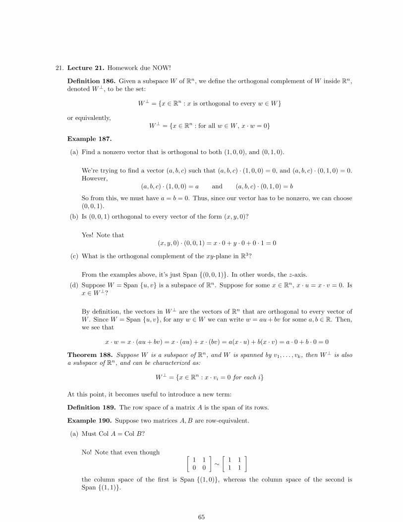
21. Lecture 21. Homework due NOW!

Definition 186. Given a subspace W of Rn, we define the orthogonal complement of W inside Rn,denoted W⊥, to be the set:

W⊥ = {x ∈ Rn : x is orthogonal to every w ∈W}

or equivalently,W⊥ = {x ∈ Rn : for all w ∈W , x · w = 0}

Example 187.

(a) Find a nonzero vector that is orthogonal to both (1, 0, 0), and (0, 1, 0).

We’re trying to find a vector (a, b, c) such that (a, b, c) · (1, 0, 0) = 0, and (a, b, c) · (0, 1, 0) = 0.However,

(a, b, c) · (1, 0, 0) = a and (a, b, c) · (0, 1, 0) = b

So from this, we must have a = b = 0. Thus, since our vector has to be nonzero, we can choose(0, 0, 1).

(b) Is (0, 0, 1) orthogonal to every vector of the form (x, y, 0)?

Yes! Note that(x, y, 0) · (0, 0, 1) = x · 0 + y · 0 + 0 · 1 = 0

(c) What is the orthogonal complement of the xy-plane in R3?

From the examples above, it’s just Span {(0, 0, 1)}. In other words, the z-axis.

(d) Suppose W = Span {u, v} is a subspace of Rn. Suppose for some x ∈ Rn, x · u = x · v = 0. Isx ∈W⊥?

By definition, the vectors in W⊥ are the vectors of Rn that are orthogonal to every vector ofW . Since W = Span {u, v}, for any w ∈W we can write w = au+ bv for some a, b ∈ R. Then,we see that

x · w = x · (au+ bv) = x · (au) + x · (bv) = a(x · u) + b(x · v) = a · 0 + b · 0 = 0

Theorem 188. Suppose W is a subspace of Rn, and W is spanned by v1, . . . , vk, then W⊥ is alsoa subspace of Rn, and can be characterized as:

W⊥ = {x ∈ Rn : x · vi = 0 for each i}

At this point, it becomes useful to introduce a new term:

Definition 189. The row space of a matrix A is the span of its rows.

Example 190. Suppose two matrices A,B are row-equivalent.

(a) Must Col A = Col B?

No! Note that even though [1 10 0

]∼[

1 11 1

]the column space of the first is Span {(1, 0)}, whereas the column space of the second isSpan {(1, 1)}.

65

(b) Must Row A = Row B?

As it turns out, yes! To see this, we analyze what happens when you perform a single elementaryrow operation:

Clearly interchanging two rows doesn’t change the span, and scaling any row by a nonzeronumber doesn’t change the span. On the other hand, suppose the rows of your matrix arecalled v1, v2, v3, and suppose we add a times v1 to v3. Then, consider the two spans:

W = Span {v1, v2, v3} V = Span {v1, v2, av1 + v3}

Clearly av1 + v3 ∈W , so certainly W ⊃ V . On the other hand, −av1 ∈ V , so (−av1) + (av1 +v3) = v3 ∈ V , so V ⊃W , so we must have V = W .

Theorem 191. If A and B are row equivalent, then Row A = Row B.

Now let A be a matrix with v1, . . . , vn as rows, ie A =

v1...

vn

. Then given a vector x, applying the

row-column rule, we see that

Ax =

v1 · x...

vn · x

From this, we see that if Ax = 0, then x must be orthogonal to every row of A! (and conversely, ifx · vi = 0 for each i, then Ax = 0).

Theorem 192. Let A be any matrix, then

(Row A)⊥ = Nul A and (Col A)⊥ = Nul AT

Example 193. Let W = Span {v1, v2, v3}, where

v1 =

1023−1

v2 =

310−1

0

v3 =

−2

15−1

1

Find a basis for W⊥.

Consider the matrix A with v1, v2, v3 as rows, namely

A =

1 0 2 3 −13 1 0 −1 0−2 1 5 −1 1

then W = Row A, so by the theorem above, we have W⊥ = (Row A)⊥ = Nul A, so we only need tofind a basis for Nul A, which is something we already know how to do.

66

Definition 194. A set of vectors {u1, . . . , up} ⊆ Rn is an orthogonal set if the vectors are pairwiseorthogonal. That is, ui · uj = 0 for all i 6= j.

Theorem 195. Any orthogonal set of nonzero vectors is linearly independent.

Proof. Suppose {u1, . . . , un} is orthogonal, then if c1u1 + · · ·+ cnun = 0, then

u1 · (c1u1 + · · ·+ cnun) = u1 · 0 = 0

but the left side is just c1u1, and so since u1 6= 0, it must be that c1 = 0. Repeating this for each cishows that u1, . . . , un is linearly independent.

Example 196. Consider the following vectors in R3.

v1 =

311

v2 =

−121

v3 =

−1/2−27/2

(a) Is this an orthogonal set?

To see if it’s an orthogonal set, you have to check to see if v1 · v2 = v1 · v3 = v2 · v3 = 0. In thiscase, all these are zero, so indeed {v1, v2, v3} is an orthogonal set.

(b) Do {v1, v2, v3} form a basis for R3?

Yes. By the preceding theorem, this set is linearly independent. Since it’s a linearly independentset of 3 vectors in the 3-dimensional space R3, it’s a basis for R3.

(c) What are the coordinates of w = (1, 1, 1) relative to this basis?

This is a problem we already know how to do. Ie, we’re just solving the vector equationw = x1v1 + x2v2 + x3v3. Another way to do this involves taking advantage of the properties oforthogonal sets.

Since v1, v2, v3 form a basis for R3, we know that there must exist c1, c2, c3 such that

w = c1v1 + c2v2 + c3v3

So now, let’s start by trying to figure out what c1 is. Now, consider dotting both sides by v1.Then, we get

v1 · w = v1 · (c1v1 + c2v2 + c3v3)

= v1 · (c1v1) + v2 · (c2v2) + v3 · (c3v3)

= c1(v1 · v1) + c2(v1 · v2) + c3(v1 · v3)

= c1‖v1‖2

Thus, we see that

c1 =v1 · w‖v1‖2

=

311

· 1

11

/ 311

· 3

11

= 5/11

Repeating this process with v2, v3, we see that

c2 =v2 · w‖v2‖2

and c3 =v3 · w‖v3‖2

67

Theorem 197. Let {u1, . . . , up} be an orthogonal basis for a subspace W of Rn, then for any w ∈W ,we have

w = c1u1 + · · ·+ cpup

where ci = w·ui

‖ui‖2 .

Proof. Since {u1, . . . , up} span W , these coefficients must exist. Thus, dotting by ui, we get:

w · ui = (c1u1 + · · · cpup) · ui = ci(ui · ui)

so ci = w·ui

‖ui‖2 .

This theorem is a special case of a more general idea.

Example 198. Suppose W is a 1-dimensional subspace of Rn, generated by w (ie, W = Span {w}),and y ∈ Rn.

(a) How could we break y down into two pieces, one that lies in W , and one that is orthogonal toW?

Ie, we want to write y = y + z, where y ∈W and z ∈W⊥.

Since z = y − y, the question is, for what y ∈W will y − y ∈W⊥?

Well, since y − y ∈ W⊥ if and only if y − y is orthogonal to w, so this is equivalent to solvingthe equation

w · (y − y) = 0

or equivalently, since y ∈ W , we can write y = αw, so we’re really asking, “for what α isw · (y − αw) = 0?”

0 = w · (y − αw) = w · y − αw · w = w · y − α‖w‖2

Thus, it must be that α = w·y‖w‖2 .

(b) Suppose W = Span {(1, 2)} ⊆ R2. Let y = (2, 1). Decompose y = y + z, where y ∈ W andz ∈W⊥.

Well, as usual, we want to find y ∈W such that y − y ∈W⊥. In other words, we want to findα ∈ R such that y − α(1, 2) ∈W⊥, ie we want to find α such that[

12

]·([

21

]− α

[12

])= 0

Thus, as usual, solving for α, we get:

0 =

[12

]·[

21

]− α

∥∥∥∥[ 12

]∥∥∥∥2 =

[12

]·[

21

]− 5α = 3− 5α

soα = 3/5

Alternatively, directly applying the formula from (a), we get

α =

[12

]·[

21

]∥∥∥∥[ 1

2

]∥∥∥∥2=

3

5

From this, we see that y =

[21

]=

3

5

[12

]︸︷︷︸

y

+

[ 21

]− 3

5

[12

]︸︷︷︸

z

.

68

22. Lecture 22. (Sections 6.2 and 6.3)

Problem Set 8 due next thursday.

Interlude on Orthonormal Sets

Definition 199. A set of vectors {u1, . . . , up} is an orthonormal set if it is an orthogonal set of unitvectors. An orthonormal basis for a vector space V is an orthonormal set that is also a basis for V .

Example 200. Consider the set

v1 =

311

, v2 =

−121

, v3 =

−1−4

7

(a) Is it an orthonormal set?

You can compute that v1 · v2 = v1 · v3 = v2 · v3 = 0. On the other hand, they are not all unitvectors (in fact, none of them are). Thus, they are not orthonormal.

(b) How could you modify v1, v2, v3 to form an orthonormal set?

Note that scaling orthogonal sets preserves the property of orthogonality. Thus, we simplyneed to scale each of the vectors by their norms, ie, the set{

1

‖v1‖v1,

1

‖v2‖v2,

1

‖v3‖v3

}is orthonormal.

Theorem 201. An m× n matrix U has orthonormal columns if and only if UTU = I.

Proof. For simplicity, suppose n = 3, then let U = [u1 u2 u3]. Consider the product

UTU =

uT1uT2uT3

[u1 u2 u3]

Corollary 202. An m× n matrix U has orthonormal rows if and only if (ask class) UUT = I.

Example 203.

(a) Suppose U is 5× 4 and has orthonormal columns. Can it have orthonormal rows? Must it?

No, because then it would be invertible. Also, if it did, then UT would be a 4× 5 matrix withorthnormal(LI) columns.

(b) Suppose U is 5× 5. Suppose it has orthonormal columns. Must it have orthonormal rows?

Yes. Since it has orthonormal columns, its columns are linearly independent, and hence sinceit’s square, it must be invertible. On the other hand, since UTU = I, its inverse is exactly UT ,so we also know that UUT = I, ie U has orthonormal rows.

Theorem 204. Let U be an m × n matrix with orthonormal columns, and let x and y be in Rn.Then, (Ux) · (Uy) = x · y.

69

Proof. Let xi, yi be the coordinates of x, y, and ui be the columns of U , then

(Ux) · (Uy) = (∑

xiui) · (∑

yiui) =∑

xiyi‖ui‖2 =∑

xiyi = x · y

Corollary 205. Let U be an m× n matrix with orthonormal columns, and let x, y ∈ Rn. Then,

(a) ‖Ux‖ = ‖x‖(b) (Ux) · (Uy) = 0 if and only if x · y = 0

Proof. For (a), recall that ‖Ux‖ = (Ux) · (Ux), but by the previous theorem, we have

(Ux) · (Ux) = x · x = ‖x‖

This proves (a). Part (b) also follows immediately from the previous theorem.

Orthogonal Projections

Last time, we considered problems like this:

Example 206. Suppose W = Span {(1, 0, 0)} ⊆ R3. Let y = (1, 1, 1). Decompose y = y+ z, wherey ∈W and z ∈W⊥.

In this case, we want to find α such that

100

·

z︷︸︸︷ 111

− α 1

00

︸︷︷︸

y

= 0

ie, 100

· 1

11

− α∥∥∥∥∥∥ 1

00

∥∥∥∥∥∥2

= 0 simplifying... 1− α = 0

So, α = 1. Indeed, we can write

y =

111

=

100

+

111

− 1

00

=

100

+

011

Here, we say that the vector y is called the orthogonal projection of y onto the 1-dimensionalsubspace W , and is denoted projW y.

Definition 207. Given a subspace W ⊆ Rn and a vector y ∈ Rn, the orthogonal projection of yonto W is denoted projW y, and is the unique vector y ∈W such that y − y ∈W⊥.

What would we do if instead W was 2-dimensional?

Example 208. Suppose W = Span {(1, 0, 0), (1, 1, 0)} ⊆ R3. Let y = (2, 2, 2). Find projW y.

As per the definition, we’re trying to find a vector y ∈W such that y − y ∈W⊥. Let

v1 =

100

, v2 =

110

70

So we see that W = Span {v1, v2}. Now, everything in W can be written as a1v1 + a2v2, so we’rereally just trying to find the coefficients a1, a2 such that 2

22

︸︷︷︸

y

−a1

100

︸︷︷︸

v1

−a2

110

︸︷︷︸

v2

∈W⊥

Once we have a1, a2, we can declare y = a1v1 + a2v2, and say z = y − y. By thm188, since W isspanned by v1, v2, it suffices to find a1, a2 such that:

222

︸︷︷︸

y

−a1

100

︸︷︷︸

v1

−a2

110

︸︷︷︸

v2

· 1

00

︸︷︷︸

v1

= 0

and 2

22

︸︷︷︸

y

−a1

100

︸︷︷︸

v1

−a2

110

︸︷︷︸

v2

· 1

10

︸︷︷︸

v2

= 0

Now, if you simplify the above two equations as much as possible, you can see that each equation isin fact a linear equation in the variables a1, a2, and so solving the two equations above is really justthe same as solving a linear system.

This method will in general work. However, we’re going to consider another method.

Example 209. Consider the problem in the previous example. Note that {(1, 0, 0), (0, 1, 0)} ={e1, e2} is an orthogonal basis for W . Now, suppose there exists y ∈W such that y− y ∈W⊥, thenwe can write y = b1e1 + b2e2. Thus, figuring out what y is is the same as determining b1, b2. So,what are b1, b2?

Let’s start with b1. To find b1, we’ll first ask, what is (y − y) · e1?

By assumption, since (y − y) ∈W⊥, it must be the case that (y − y) · e1 = 0. Thus, we have

0 = (y − y) · e1= y · e1 − y · e1= y · e1 − (b1e1 + b2e2) · e1= y · e1 − b1e1 · e1 − b2e2 · e1= y · e1 − b1‖e1‖2 − b2(e2 · e1)

however, since {e1, e2} form an orthogonal basis for W , we see that e2 · e1 = 0, so:

0 = · · · = y · e1 − b1‖e1‖2

Thus, doing this for b2 as well will show that

b1 =y · e1‖e1‖2

, b2 =y · e2‖e2‖2

In fact, you can verify that

y − y · e1‖e1‖2

e1 −y · e2‖e2‖2

e2 ∈W⊥

Note that here, we used the crucial fact that {e1, e2} formed an orthogonal basis for W . In fact, ingeneral, we have:

71

Theorem 210. Suppose W ⊆ Rn is a subspace, and {u1, . . . , up} is an orthogonal basis for W .Then for any y ∈ Rn, we can find y, z such that y ∈W , z ∈W⊥, and y = y+ z. Here, by definitiony = projW y. In fact, we have the following formula for y = projW y:

y = projW y =y · u1‖u1‖2

u1 + · · ·+ y · up‖up‖2

up

With notation as in the theorem above, let Wi = Span {ui}. Note that these vectors y·ui

‖ui‖2uiare in fact the vectors projWi

y. Essentially, the way we construct y, is by projecting y onto each“one-dimensional axis” of W , and then adding all the components together.

Note that the above theorem is only useful if we can find an orthogonal basis for W . We’ll discussnext week how to find orthogonal bases.

Example 211. Let W ⊆ Rn be a subspace, and y ∈W . What is projW y?

Recall, we’re just trying to find the vector y ∈W such that y− y ∈W⊥. However, since y ∈W , wecan pick y = y, in which case we have y − y = 0, which is trivially in W⊥.

Thus, we see that if y ∈W , we have projW y = y.

Theorem 212. (Best Approximation Theorem) Let W be a subspace of Rn, and let y ∈ Rn. Lety = projW y, then for all v ∈W with v 6= y, we have

‖y − y‖ < ‖y − v‖

Proof. Clearly y − v ∈ W , and by definition of orthogonal projection, y − y ∈ W⊥ and hence isorthogonal to y− v. Thus, by the pythagorean theorem (if x · y = 0, then ‖x+ y‖2 = ‖x‖2 + ‖y2‖ =‖x− y‖2), we see that.

‖y − v‖2 = ‖(y − y) + (y − v)‖2 = ‖y − y‖2 + ‖y − v‖2

Thus ‖y − v‖2 − ‖y − y‖2 = ‖y − v‖2 > 0, which shows that ‖y − v‖ > ‖y − y‖.

Note that this ensures that projW y is in fact unique and well-defined.

Lastly, we have this following fact. The proof is in the book (thm 10, page 351), but it’s really aspecial case that isn’t very interesting imo.

Theorem 213. If {u1, . . . , up} is an orthonormal basis for a subspace W of Rn, then

projW y = (y · u1)u1 + (y · u2)u2 + · · ·+ (y · up)up

If U = [u1 u2 · · · up], thenprojW y = UUT y

for all y ∈ Rn.

72

23. Lecture 23. Gram-Schmidt (Section 6.4)

Example 214. We’ll develop this procedure inductively.

(a) We’ll start with the base case: Suppose W is a 1-dimensional subspace of Rn, say W =Span {x1}. What is an orthgonal basis for W?

In this case, {x1} is itself an orthogonal basis for W ! Note that since W is 1-dimensional,x1 6= 0, so {x1} is a linearly independent (and orthogonal) set, that in this case spans W , henceit’s an orthogonal basis for W .

(b) Now suppose W is a k-dimensional space, and v1, . . . , vk is an orthogonal basis for W . Furthersuppose V is a (k+ 1)-dimensional space that contains W , and suppose v is a vector such thatv ∈ V but v /∈W .

How would you find an orthogonal basis for V ?

Hint: Note that we’ve already got an orthogonal basis for W , namely {v1, . . . , vk}. How couldwe find a vk+1 such that {v1, . . . , vk, vk+1} is an orthogonal basis for V ?

Indeed, we’re looking for a nonzero vector vk+1 ∈ V such that vk+1 is orthogonal to v1, . . . , vk.How could we find such a vector?

Hint: How can you “extract” such a vector vk+1 from the vector v?

We know we can write v = projW v + z, where z ∈ W⊥. Since projW v ∈ W , and v /∈ W , itmust be the case that z 6= 0. Thus, z is a nonzero vector that is orthogonal to all of W , and inparticular to v1, . . . , vk. Thus, the set

{v1, . . . , vk, z}

is an orthogonal set of nonzero vectors in V , and hence they are linearly independent. Onthe other hand, there are k + 1 vectors there, and V is (k + 1)- dimensional, so they form anorthogonal basis of V that extends the orthogonal basis for W .

The general process can be summarized as follows:

Algorithm 215. (Gram-Schmidt)

(a) Given one-dimensional space W , let v1 ∈ W be any nonzero vector. Then {v1} forms anorthogonal basis of W .

(b) Suppose W is a k-dimensional space with orthogonal basis {v1, . . . , vk}, and suppose V ) Wis a (k + 1)-dimensional space containing W , then we can find a vector vk+1 ∈ V such that{v1, . . . , vk, vk+1} is an orthogonal basis for V . This is accomplished as follows:

(i) Since V is strictly larger than W , it’s possible to find some vector v ∈ V with v /∈W . Findsuch a v.

(ii) Given such a v as above, we know that we can write

v = projW v + z

where by definition projW v ∈ W and z ∈ W⊥. Since {v1, . . . , vk} is an orthogonal basisfor W , we can apply thm210 to compute projW v as follows:

projW v =v · v1‖v1‖2

v1 +v · v2‖v2‖2

v2 + · · ·+ v · vk‖vk‖2

vk

Now we may compute z = v − projW v ∈ W⊥. Since v /∈ W and projW v ∈ W , it must bethe case that z 6= 0. Thus, setting vk+1 := z, we see that

{v1, . . . , vk, vk+1}

indeed gives us an orthogonal set of (k + 1) nonzero vectors in V . Since they are orthog-onal and nonzero, the set is linearly independent, so since dim V = k + 1, they form anorthogonal basis for V .

73

Now we’ll apply this method to a few explicit examples.

Example 216. Consider the vectors

x1 =

11−1

, x2 =

132

, x3 =

210

(a) Is {x1, x2, x3} a basis for R3?

Yes. The matrix [x1 x2 x3] is a 3× 3 matrix with 3 pivots, so its columns are a basis for R3.

(b) Find an orthogonal basis for W1 = Span {x1}.

Let v1 := x1, then previous example shows that

{v1} = {x1} =

1

1−1

is itself an orthogonal basis for W1.

(c) Find an orthogonal basis for W2 = Span {x1, x2}.

Now we’re in case (b) of the previous example. Here, W1 is our k-dimensional space (in thiscase k = 1), with orthogonal basis {v1}.In this case, since {x1, x2} are linearly independent, we see that x2 /∈ W1 = Span {v1}, andhence x2 plays the role of the vector v in case the previous example. Thus, we want to writex2 = projW1

x2 + z.

To do this, we must first compute projW1x2. To do this, we refer to thm210. The theorem tells

us that since {v1} is an orthogonal basis for W1,

projW1x2 =

x2 · v1‖v1‖2

v1 =2

3

11−1

=

2/32/3−2/3

Thus, solving for z, we get:

z = x2 − projW1x2 = x2 −

x2 · v1‖v1‖2

v1 =

132

− 2/3

2/3−2/3

=

1/37/38/3

We know from the definition of projW1

x2 that z is orthogonal to v1, and hence setting

v2 = z =

1/37/38/3

,we see that {v1, v2} is now an orthogonal basis for W2.

(d) Find an orthogonal basis for W3 = Span {x1, x2, x3} = R3.

Again we’re in case (b) of the previous example, where k = 2. Here, W2 = Span {x1, x2} is ourk-dimensional space, with orthogonal basis {v1, v2}.Now, again since {x1, x2, x3} are linearly independent, x3 /∈W2, and hence we want to extractthe perpendicular component from it to form v3. To do this, again we use thm210 to calculate

projW2x3 =

x3 · v1‖v1‖2

v1 +x3 · v2‖v2‖2

v2 =3

3

11−1

+3

38/3

1/37/38/3

=

11−1

+9

38

1/37/38/3

74

Thus, by the definition of projW2x3, we know that the vector

z = x3 − projW2x3 =

210

− 1

1−1

+9

38

1/37/38/3

is orthogonal to W2, and hence in particular it is orthogonal to v1, v2. Furthermore, z 6= 0, soif we set

v3 = z =

210

− 1

1−1

+9

38

1/37/38/3

we see that

{v1, v2, v3}

is an orthogonal set of 3 nonzero vectors in the 3-dimensional space W3 = R3, and hence theyform an orthogonal basis for W3.

Corollary 217. In general, given a basis {x1, . . . , xp} for a vector space W , define

v1 = x1

v2 = x2 −x2 · v1‖v1‖2

v1

v3 = x3 −x3 · v1‖v1‖2

v1 −x3 · v2‖v2‖2

v2

...

vp = xp −xp · v1‖v1‖2

v1 −xp · v2‖v2‖2

v2 − · · · −xp · vp−1‖vp−1‖2

vp−1

then {v1, . . . , vp} is an orthogonal basis for W .

Colors

So far, we’ve only thought of vector spaces in two contexts - either as solution sets of linear systems,or geometric “spaces”, like the line, the plane, or 3-space. In fact, the kinds of vector spaces thatappear in science and mathematics form a far more varied lot than the paltry few we’ve considered.Today, we’ll consider one of these weird/crazy/awesome vector spaces.

We know that there are 3 primary colors. What does that mean? It means, that by combiningsuitable quantities of each of the three primary colors, we can achieve any color that we want.Indeed, this is beginning to sound exactly like the definition of what it means for a vector space tobe 3-dimensional. In this sense, then, the space of colors is 3-dimensional. Indeed, you can scalecolors (in the sense that you can increase/decrease the intensity of the colors), and you can addcolors (by combining them), so it makes sense to call the space of colors, under the two operationsof scaling and combining (read: multiplication by scalars and addition), a vector space!

Since it’s 3-dimensional, as it turns out it’s isomorphic to R3, in the following sense:

If we view the vector rgb

∈ R3

as representing the color obtained by combining r-amounts of red, g-amounts of green, and b-amountsof blue, where r, g, b ∈ R, we can view points in R3 as colors!

On the other hand, what are colors really? Well, fundamentally speaking, a “color” is just a formof visible light, and in fact, if we want to distinguish, say, light red from dark red, we should reallyidentify color with all the data associated to a light wave (not just its frequency).

75

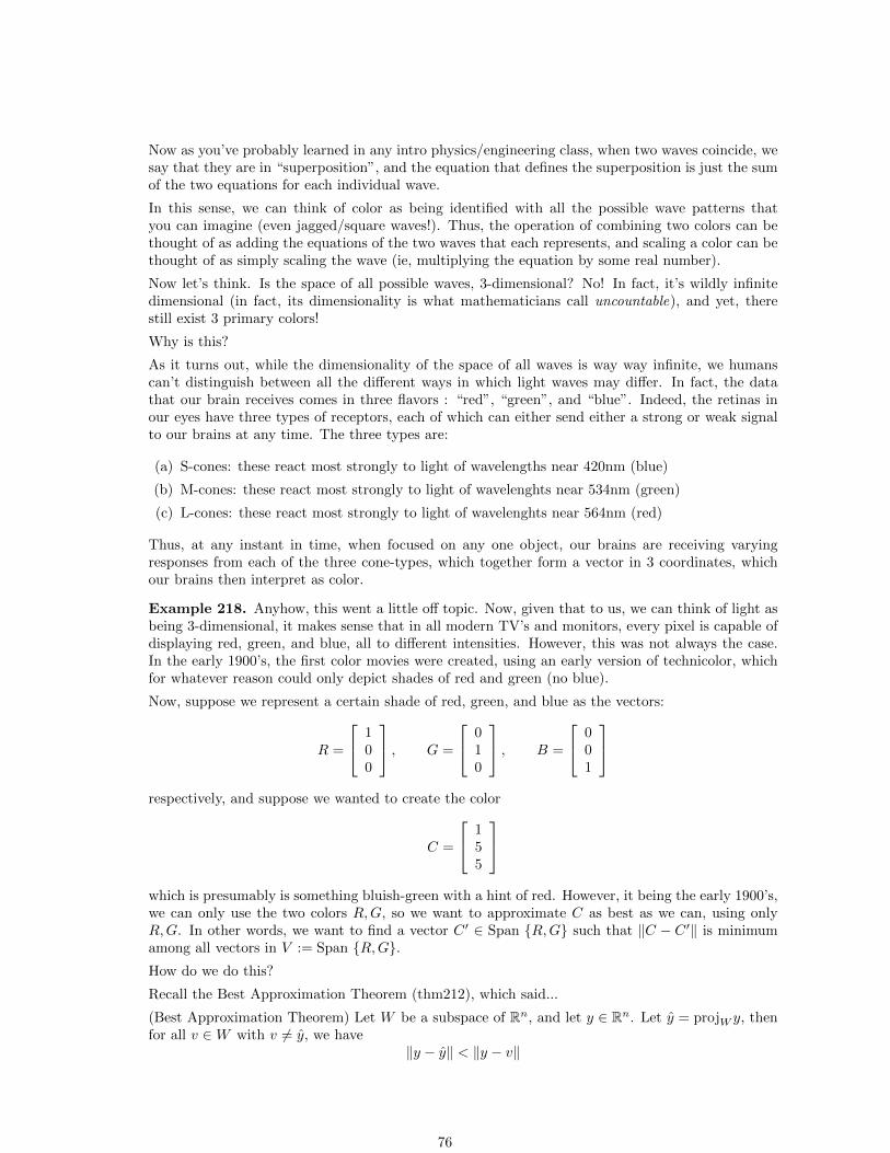
Now as you’ve probably learned in any intro physics/engineering class, when two waves coincide, wesay that they are in “superposition”, and the equation that defines the superposition is just the sumof the two equations for each individual wave.

In this sense, we can think of color as being identified with all the possible wave patterns thatyou can imagine (even jagged/square waves!). Thus, the operation of combining two colors can bethought of as adding the equations of the two waves that each represents, and scaling a color can bethought of as simply scaling the wave (ie, multiplying the equation by some real number).

Now let’s think. Is the space of all possible waves, 3-dimensional? No! In fact, it’s wildly infinitedimensional (in fact, its dimensionality is what mathematicians call uncountable), and yet, therestill exist 3 primary colors!

Why is this?

As it turns out, while the dimensionality of the space of all waves is way way infinite, we humanscan’t distinguish between all the different ways in which light waves may differ. In fact, the datathat our brain receives comes in three flavors : “red”, “green”, and “blue”. Indeed, the retinas inour eyes have three types of receptors, each of which can either send either a strong or weak signalto our brains at any time. The three types are:

(a) S-cones: these react most strongly to light of wavelengths near 420nm (blue)

(b) M-cones: these react most strongly to light of wavelenghts near 534nm (green)

(c) L-cones: these react most strongly to light of wavelenghts near 564nm (red)

Thus, at any instant in time, when focused on any one object, our brains are receiving varyingresponses from each of the three cone-types, which together form a vector in 3 coordinates, whichour brains then interpret as color.

Example 218. Anyhow, this went a little off topic. Now, given that to us, we can think of light asbeing 3-dimensional, it makes sense that in all modern TV’s and monitors, every pixel is capable ofdisplaying red, green, and blue, all to different intensities. However, this was not always the case.In the early 1900’s, the first color movies were created, using an early version of technicolor, whichfor whatever reason could only depict shades of red and green (no blue).

Now, suppose we represent a certain shade of red, green, and blue as the vectors:

R =

100

, G =

010

, B =

001

respectively, and suppose we wanted to create the color

C =

155

which is presumably is something bluish-green with a hint of red. However, it being the early 1900’s,we can only use the two colors R,G, so we want to approximate C as best as we can, using onlyR,G. In other words, we want to find a vector C ′ ∈ Span {R,G} such that ‖C − C ′‖ is minimumamong all vectors in V := Span {R,G}.How do we do this?

Recall the Best Approximation Theorem (thm212), which said...

(Best Approximation Theorem) Let W be a subspace of Rn, and let y ∈ Rn. Let y = projW y, thenfor all v ∈W with v 6= y, we have

‖y − y‖ < ‖y − v‖

76

Indeed, this tells us that the closest vector in Span {R,G} to C is just projV C. In this case, this iseasy to compute. Since R,G are an orthogonal basis for V , we can use thm210 to compute projV Cas follows:

projV C =C ·R‖R‖2

R+C ·G‖G‖2

G =1

1

100

+5

1

010

=

150

Not surprisingly, the closest vector in the “xy-plane” to (1, 5, 5) is just (1, 5, 0).

Of course, this was just a toy example. The full power in the best approximation theorem, and infact in everything that we’ve learned so far, is their ability to generalize, build upon each other, andprovide context and understanding for the specific cases we’re already familiar with, and in doingso shed light on the mysterious and unfamiliar territory where all the booty is buried.

77

Math 220 F11 Lecture Notes - Department of Mathematics · Math 220 F11 Lecture Notes William Chen...

Documents

Transcript of Math 220 F11 Lecture Notes - Department of Mathematics · Math 220 F11 Lecture Notes William Chen...