MATH 154. ALGEBRAIC NUMBER THEORYmath.stanford.edu/~conrad/154Page/handouts/undergraduate-number...
153
MATH 154. ALGEBRAIC NUMBER THEORY LECTURES BY BRIAN CONRAD, NOTES BY AARON LANDESMAN CONTENTS 1. Fermat’s factorization method 2 2. Quadratic norms 8 3. Quadratic factorization 14 4. Integrality 20 5. Finiteness properties of O K 26 6. Irreducible elements and prime ideals 31 7. Primes in O K 37 8. Discriminants of number fields 41 9. Some monogenic integer rings 48 10. Prime-power cyclotomic rings 54 11. General cyclotomic integer rings 59 12. Noetherian rings and modules 64 13. Dedekind domains 69 14. Prime ideal factorization 74 15. Norms of ideals 79 16. Factoring pO K : the quadratic case 85 17. Factoring pO K : the general case 88 18. Ramification 93 19. Relative factorization and rings of fractions 96 20. Localization and prime ideals 101 21. Applications of localization 105 22. Discriminant ideals 110 23. Decomposition and inertia groups 116 24. Class groups and units 122 25. Computing some class groups 128 26. Norms and volumes 134 27. Volume calculations 138 28. Minkowski’s theorem and applications 144 29. The Unit Theorem 148 References 153 Thanks to Nitya Mani for note-taking on two days when Aaron Landesman was away. 1
-
Upload
nguyenlien -
Category
Documents
-
view
224 -
download
1
Transcript of MATH 154. ALGEBRAIC NUMBER THEORYmath.stanford.edu/~conrad/154Page/handouts/undergraduate-number...

MATH 154. ALGEBRAIC NUMBER THEORY
LECTURES BY BRIAN CONRAD, NOTES BY AARON LANDESMAN
CONTENTS
1. Fermat’s factorization method 22. Quadratic norms 83. Quadratic factorization 144. Integrality 205. Finiteness properties of OK 266. Irreducible elements and prime ideals 317. Primes in OK 378. Discriminants of number fields 419. Some monogenic integer rings 4810. Prime-power cyclotomic rings 5411. General cyclotomic integer rings 5912. Noetherian rings and modules 6413. Dedekind domains 6914. Prime ideal factorization 7415. Norms of ideals 7916. Factoring pOK: the quadratic case 8517. Factoring pOK: the general case 8818. Ramification 9319. Relative factorization and rings of fractions 9620. Localization and prime ideals 10121. Applications of localization 10522. Discriminant ideals 11023. Decomposition and inertia groups 11624. Class groups and units 12225. Computing some class groups 12826. Norms and volumes 13427. Volume calculations 13828. Minkowski’s theorem and applications 14429. The Unit Theorem 148References 153
Thanks to Nitya Mani for note-taking on two days when Aaron Landesman was away.1

2 BRIAN CONRAD AND AARON LANDESMAN
1. FERMAT’S FACTORIZATION METHOD
Today we will discuss the proof of the following result, and highlightsome of its main ideas that will be important themes in the course:
Theorem 1.1 (Fermat). For x, y ∈ Z, the only solutions of y2 = x3 − 2 are(3,±5).
Remark 1.2. This is an elliptic curve (a notion we shall not define, essentiallythe set of solutions to a certain type of cubic equation in two variables) withinfinitely many Q-points, a contrast with finiteness of its set of Z-points.
Fermat’s equation can be rearranged into the form x3 = y2 + 2.
Lemma 1.3. For any Z-solution (x, y) to x3 = y2 + 2, the value of y must be odd.
Proof. Indeed, if y is even then x is even, so x3 is divisible by 8. But y2 + 2 =4k + 2 is not divisible by 8. �
Fermat’s first great idea is to introduce considerations in the ring
Z[√−2] := {m + n
√−2 |m, n ∈ Z}.
The point is that over this ring, the equation
x3 = y2 + 2
can be expressed as
x3 = (y +√−2)(y−
√−2).
To find solutions to this, we ask the following two questions:
Question 1.4. Do y +√−2 and y−
√−2 have “gcd = 1” (meaning no non-
trivial factor in common, where “nontrivial” means “not a unit”)?
Question 1.5. If we know the answer to the above question is “yes,” can weconclude that both y±
√−2 are cubes in Z[
√−2]?
Recall the definition of unit:
Definition 1.6. For R a commutative ring, an element u ∈ R is a unit if thereexists u′ ∈ R, so that uu′ = 1. We let
R× := { units in R};this is an abelian group.
Example 1.7. (1) Z× = {±1}.(2) For F a field, F× = F− {0} by the definition of a field.
MATH 154. ALGEBRAIC NUMBER THEORY 3
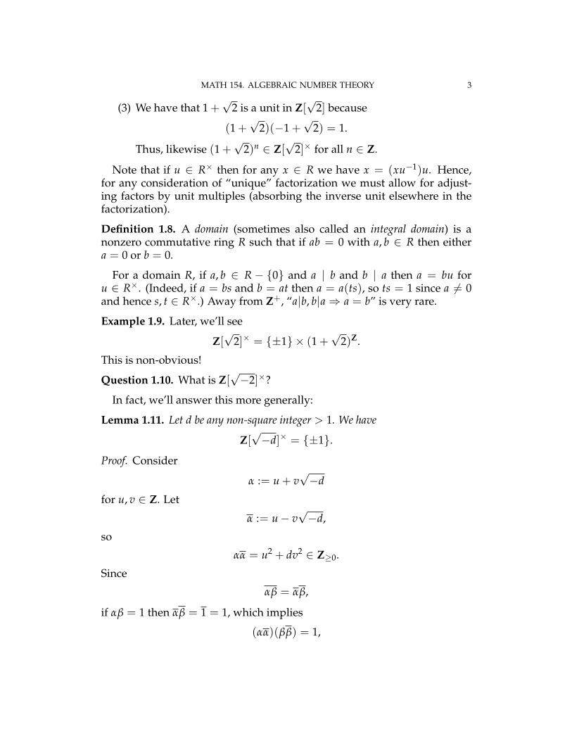
(3) We have that 1 +√
2 is a unit in Z[√
2] because
(1 +√
2)(−1 +√
2) = 1.
Thus, likewise (1 +√
2)n ∈ Z[√
2]× for all n ∈ Z.
Note that if u ∈ R× then for any x ∈ R we have x = (xu−1)u. Hence,for any consideration of “unique” factorization we must allow for adjust-ing factors by unit multiples (absorbing the inverse unit elsewhere in thefactorization).
Definition 1.8. A domain (sometimes also called an integral domain) is anonzero commutative ring R such that if ab = 0 with a, b ∈ R then eithera = 0 or b = 0.
For a domain R, if a, b ∈ R − {0} and a | b and b | a then a = bu foru ∈ R×. (Indeed, if a = bs and b = at then a = a(ts), so ts = 1 since a 6= 0and hence s, t ∈ R×.) Away from Z+, “a|b, b|a⇒ a = b” is very rare.
Example 1.9. Later, we’ll see
Z[√
2]× = {±1} × (1 +√
2)Z.
This is non-obvious!
Question 1.10. What is Z[√−2]×?
In fact, we’ll answer this more generally:
Lemma 1.11. Let d be any non-square integer > 1. We have
Z[√−d]× = {±1}.
Proof. Consider
α := u + v√−d
for u, v ∈ Z. Let
α := u− v√−d,
so
αα = u2 + dv2 ∈ Z≥0.
Since
αβ = αβ,
if αβ = 1 then αβ = 1 = 1, which implies
(αα)(ββ) = 1,

4 BRIAN CONRAD AND AARON LANDESMAN
so
αα = 1
because αα = u2 + dv2 ∈ Z≥0. The equality u2 + dv2 = 1 with d > 1 forcesv = 0 and then u = ±1. �
Remark 1.12. If we try the same argument for Z[√
d], we get u2− dv2 = ±1with u, v ∈ Z (and v 6= 0 for units distinct from±1). The question of findingsuch non-trivial units then becomes Pell’s equation, which is
u2 − dv2 = 1
and its variant with −1 on the right side. For the case d = 2, Pell’s equationhas infinitely many Z-solutions with u, v > 0 (as we will recover later in thecourse from a more sophisticated point of view), beginning with:
(3, 2), (17, 12), . . .
by considering powers (1 +√
2)2n = (3 + 2√
2)n for n > 0.The variant equation u2 − 2v2 = −1 also has infinitely many Z-solutions
with u, v > 0 by considering (1 +√
2)2n+1 with n ≥ 0, such as:
(1, 1), (7, 5), . . .
We’ll now resume our goal of finding the Z-solutions to x3 = y2 + 2,first addressing if y±
√−2 have a non-unit common factor. The answer is
negative:
Lemma 1.13. If δ ∈ Z[√−2] satisfies
δ | (y +√−2) and δ | (y−
√−2)
then δ is a unit.
Proof. First, recall from Lemma 1.3 that y is odd. Observe that
δ | (y +√−2)− (y−
√−2)
= 2√−2
= (√−2)3.
Then, we claim the following sublemma:
Lemma 1.14. The element√−2 ∈ Z[
√−2] is irreducible (i.e., it is a nonzero
non-unit such that any factorization as αβ must have α or β a unit).
Proof. Assuming√−2 = αβ, we have −
√−2 = αβ by conjugating both
sides. Multiplying these relations, 2 = (αα)(ββ) ∈ Z≥0, so αα = 1 orββ = 1. This implies either α or β is a unit, as desired. �

MATH 154. ALGEBRAIC NUMBER THEORY 5
In HW1 it will be shown that Z[√−2] is a UFD, so the irreducibility of√
−2 forces δ = u√−2
efor some 0 ≤ e ≤ 3 and some unit u ∈ Z[
√−2].
Thus, if δ is not a unit then√−2 | δ. Hence, to get a contradiction (and
conclude δ is a unit) it is enough to show√−2 - (y +
√−2) in Z[
√−2].
Suppose for some u, v ∈ Z that
y +√−2 =
√−2(u + v
√−2)
= 2v + u√−2.
This forces y = 2v to be even, but y is odd by Lemma 1.3. This concludesthe proof that δ is a unit. �
We conclude that in the UFD Z[√−2] we have
gcd(y +√−2, y−
√−2) = 1.
This completes the preparations for:
Proof of Theorem 1.1. In any UFD, any nonzero element is a finite product ofirreducibles, and by lumping together any irreducibles that agree up to unitmultiple we can rewrite such a product as
u ·∏i
πeii
with πi pairwise non-associate irreducible elements (non-associate meansone is not a unit times another; by irreducibility of the πi’s, this amountsto saying πi - πj for any i 6= j).
Since
(y +√−2)(y−
√−2) = x3
with
gcd(y +√−2, y−
√−2) = 1,
it follows from expressing each of
y±√−2
as a unit multiple of a product of pairwise non-associate irreducibles thatall irreducible factors of y ±
√−2 occur with multiplicity divisible by 3.
Therefore, y±√−2 is the product of a unit and a cube. But now a miracle
occurs: we know the units of Z[√−2] by Lemma 1.11, and from this we see
that all units are themselves cubes (as −1 = (−1)3)! Hence,
y +√−2 = (a + b
√−2)3
for some a, b ∈ Z.

6 BRIAN CONRAD AND AARON LANDESMAN
Therefore,
y +√−2 = (a + b
√−2)3
= a(a2 − 6b2) + b(3a2 − 2b2)√−2,
so
1 = b(3a2 − 2b2),
from which we see that b = ±1, so b2 = 1. This implies ±1 = 3a2 − 2 so
3a2 = 2± 1.
Then 3a2 equals either 3 or 1. The latter is impossible because we cannothave 3a2 = 1 with a ∈ Z. Thus, 3a2 = 3, so a = ±1. This implies b = 1, so
y = a(a2 − 6b2)
= ±(1− 6)= ±5
and x3 = y2 + 2 = 27, so x = 3, concluding the proof. �
The above considerations yield the following lessons:(1) For studying Z-solutions to polynomial equations, it’s useful to con-
sider arithmetic in larger number systems. For example, in this case,it was useful to work in Z[
√−2].
(2) We have to know about unique factorization and units in such num-ber systems. For example, in this case, we got lucky that all elementsin
Z[√−2]× = {±1}
are cubes. This is quite false for Z[√
2] since (as we’ll see later)
Z[√
2]× = (±1)× (1 +√
2)Z;
e.g., 1 +√
2 is a non-cube unit. The need to grapple with non-cubeunits makes it much harder to analyze the Z-solutions to the varianty2 = x3 + 2 of Fermat’s equation because it is harder to determinethe structure of the relevant unit group.
Let’s now consider another question of unique factorization in an imagi-nary quadratic situation.
Example 1.15. Is Z[√−3] a unique factorization domain? By Lemma 1.11,
the only units are {±1}. We can write
4 = 2 · 2
MATH 154. ALGEBRAIC NUMBER THEORY 7
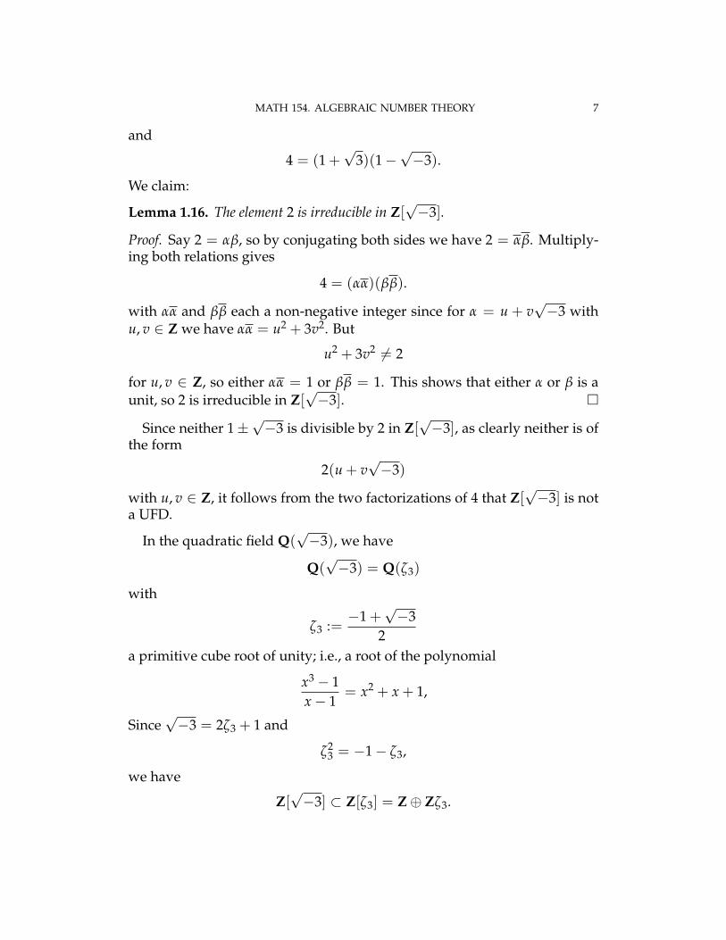
and
4 = (1 +√
3)(1−√−3).
We claim:
Lemma 1.16. The element 2 is irreducible in Z[√−3].
Proof. Say 2 = αβ, so by conjugating both sides we have 2 = αβ. Multiply-ing both relations gives
4 = (αα)(ββ).
with αα and ββ each a non-negative integer since for α = u + v√−3 with
u, v ∈ Z we have αα = u2 + 3v2. But
u2 + 3v2 6= 2
for u, v ∈ Z, so either αα = 1 or ββ = 1. This shows that either α or β is aunit, so 2 is irreducible in Z[
√−3]. �
Since neither 1±√−3 is divisible by 2 in Z[
√−3], as clearly neither is of
the form
2(u + v√−3)
with u, v ∈ Z, it follows from the two factorizations of 4 that Z[√−3] is not
a UFD.
In the quadratic field Q(√−3), we have
Q(√−3) = Q(ζ3)
with
ζ3 :=−1 +
√−3
2a primitive cube root of unity; i.e., a root of the polynomial
x3 − 1x− 1
= x2 + x + 1,
Since√−3 = 2ζ3 + 1 and
ζ23 = −1− ζ3,
we have
Z[√−3] ⊂ Z[ζ3] = Z⊕ Zζ3.

8 BRIAN CONRAD AND AARON LANDESMAN
We’ll later prove that the domain Z[ζ3] is a UFD. Thus, although Z[√−3]
fails to be a UFD, perhaps it is also the “wrong” ring to consider when con-templating “arithmetic” inside Q(
√−3); that is, it seems that Z[ζ3] is a bet-
ter ring to use. But how can one arrive at this determination in a systematicway? More broadly:
Question 1.17. For K/Q a finite extension, what is the “correct” notion of“ring of integers” for K?
Remark 1.18. Euler’s proof of Fermat’s Last Theorem for exponent 3 as-sumed that Z[
√−3] is a UFD (which is of course false by Example 1.15!)
This proof can be fixed by working in Z[ζ3].The proof of Fermat’s Last Theorem for exponent 4 is [Samuel, §1.2], af-
ter which the essential case for proving Fermat’s Last Theorem is that withexponent an odd prime p. If zp = xp + yp for p > 2 prime then
yp = zp − xp = ∏(z− ζjpx)
with ζp a primitive pth root of unity. In general, it will turn out that
Z[ζp]×
is infinite whenever p > 3, and rather beyond the scope of this course isthe fact that Z[ζp] is not a UFD whenever p > 19. Nonetheless, we will seethat Z[ζp] is the correct notion of “ring of integers” for the field Q(ζp), anddespite its failure to be a UFD in general it does have a lot of nice structuralfeatures that allow one to make serious progress on Fermat’s Last Theoremfor lots of p (and the final solution by Wiles uses techniques of a much moreadvanced nature, though building very much on the classic ideas of alge-braic number theory to be developed in this course).
2. QUADRATIC NORMS
Last time, we discussed Z-solutions to
y2 = x3 − 2
which we saw were (3,±5) via factoring in a suitable subring of the fieldQ(√−2). It turns out that the only Z-solutions to
y2 = x3 + 2
are (−1,±1) via factorization in the subring Z[√
2] ⊂ Q(√
2). This is harderto prove, but follows with some work once one shows
Z[√
2]× = ±(1 +√
2)Z.

MATH 154. ALGEBRAIC NUMBER THEORY 9
To tackle these problems, we need a way to show rings such as Z[ñ2]
are UFD’s. The most rudimentary way to do this is via the notion of Eu-clidean domain (since Euclidean domains are PID’s, hence are UFD’s).
Euclidean domains essentially are only used in first courses in algebra,and once one develops more algebraic tools, one can more easily show awider class of rings are PID’s whereas many rings we encounter in numbertheory that are PID’s turn out not to be Euclidean domains.
The Euclidean-domain approach will work for some rings like Z[i] andZ[ñ2], but quickly runs out of steam for the study of Q(
√d) with square-
free d ∈ Z once |d| grows beyond a small set of values.We next review the definition of Euclidean domain:
Definition 2.1. A domain R is Euclidean if it admits a function
ν : R→ Z≥0
(which is not necessarily multiplicative) so that
(1) ν(x) = 0 ⇐⇒ x = 0,(2) For any a, b ∈ R with b 6= 0, there exist q, r ∈ R so that a = bq + r
with ν(r) < ν(b).
Remark 2.2. There is no uniqueness assumption for q, r in the second con-dition of Definition 2.1.
Example 2.3. Take R = Z, ν(x) = |x|. Then, one could use the “greedy”division algorithm, with −b/2 ≤ r ≤ b/2. In this case r is not alwaysunique (namely, b/2 can be exchanged for −b/2 when b is even, at the costof changing q by 1).
Example 2.4. If R = k[t] over a field k, define
ν( f ) = deg f .
This is not quite a function satisfying the definition of Euclidean domainbecause ν takes value 0 on the non-zero constants too, but those are unitsand so it is not a real obstacle to extracting the PID conclusion; one mightcall such a situation “pseudo-Euclidean.”
Definition 2.5. We say Z[√
d] ⊂ Q(√
d) is norm-Euclidean if it is Euclideanwith respect to the map
ν(x) = |N(x)| := xx,
with x 7→ x the nontrivial element of Gal(Q(√
d)/Q).
10 BRIAN CONRAD AND AARON LANDESMAN
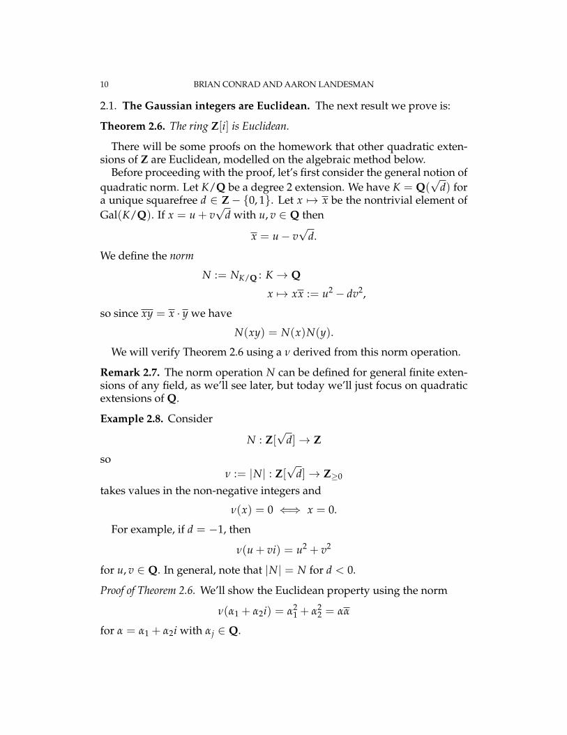
2.1. The Gaussian integers are Euclidean. The next result we prove is:
Theorem 2.6. The ring Z[i] is Euclidean.
There will be some proofs on the homework that other quadratic exten-sions of Z are Euclidean, modelled on the algebraic method below.
Before proceeding with the proof, let’s first consider the general notion ofquadratic norm. Let K/Q be a degree 2 extension. We have K = Q(
√d) for
a unique squarefree d ∈ Z− {0, 1}. Let x 7→ x be the nontrivial element ofGal(K/Q). If x = u + v
√d with u, v ∈ Q then
x = u− v√
d.
We define the norm
N := NK/Q : K → Q
x 7→ xx := u2 − dv2,
so since xy = x · y we have
N(xy) = N(x)N(y).
We will verify Theorem 2.6 using a ν derived from this norm operation.
Remark 2.7. The norm operation N can be defined for general finite exten-sions of any field, as we’ll see later, but today we’ll just focus on quadraticextensions of Q.
Example 2.8. Consider
N : Z[√
d]→ Z
soν := |N| : Z[
√d]→ Z≥0
takes values in the non-negative integers and
ν(x) = 0 ⇐⇒ x = 0.
For example, if d = −1, then
ν(u + vi) = u2 + v2
for u, v ∈ Q. In general, note that |N| = N for d < 0.
Proof of Theorem 2.6. We’ll show the Euclidean property using the norm
ν(α1 + α2i) = α21 + α2
2 = αα
for α = α1 + α2i with αj ∈ Q.

MATH 154. ALGEBRAIC NUMBER THEORY 11
The idea of the proof is the following: if we are to have a = bq + r withν(r) < ν(b) for some q, r ∈ Z[i] then
Q(i) 3 ab= q +
rb
,
with q ∈ Z[i] and r/b at distance < 1 from 0 since ν(r/b) = ν(r)/ν(b) < 1.This motivates the geometric idea to construct q and r: we try to take q to bethe point in the lattice Z[i] = Z⊕ Zi nearest to a/b ∈ Q(i) ⊂ C.
In algebraic terms, sinceab∈ Q(i) = Q[i] = {u + iv | u, v ∈ Q}
we can writeab= t1 + t2i
with t1, t2 ∈ Q, so if qj ∈ Z is the nearest integer to tj ∈ Q (breaking tiesarbitrarily) then
tj = qj + ε j
with qj ∈ Z and |ε j| ≤ 12 . Then,
ab= (q1 + q2i) + (ε1 + ε2i) = q + ε
for q ∈ Z[i] and |ε j| ≤ 12 . Hence, multiplying through by b gives a = bq + r
with
r := εb = a− bq ∈ Z[i].
By multiplicativity of the norm Q(i)→ Q, we have
ν(r) = ν(ε)ν(b) < ν(b)
because
ν(ε) = ε21 + ε2
2 ≤14+
14= 1/2.
�
Warning 2.9. The very last step that
ν(ε) = ε21 + ε2
2 ≤14+
14= 1/2.
breaks when we try to adapt it to Z[√−d] for d moderately larger (such as
all d ≥ 3) because
ν(ε) ≤ 1/4 + d/4

12 BRIAN CONRAD AND AARON LANDESMAN
and this upper bound is not generally below 1 anymore (but we barelyscrape by successfully for Z[
√−2]).
Last time it was shown that for non-square integers d > 1, we have
Z[√−d]× = {±1}.
We can make a similar, but slightly different statement when d = 1 as fol-lows. When d = 1 there are some additional units, namely ±i, but nothingmore:
Lemma 2.10. We have
Z[i]× = {±1,±i}.
Proof. Suppose
α = α1 + α2i ∈ Z[i]×
with α1, α2 ∈ Z. Then, there exists β ∈ Z[i] with
αβ = 1.
by definition of unit. Taking norms, we have
N(α)N(β) = N(1) = 1
in Z≥0 since
N(u + iv) = u2 + v2.
This forces N(α) = 1, so α21 + α2
2 = 1. One can then see that either α1 = 0 orα2 = 0, implying
α ∈ {±1,±i}.
�
Remark 2.11. As a variant, we’ll see in Exercise 2(i) of Homework 2 that inR = Z[ζ3] we have
R× = {±1,±ζ3,±ζ23}.
2.2. Factoring in quadratic UFD’s using the norm. Let’s now use the normto help with factoring in a quadratic UFD.
Example 2.12. Let’s find the prime factorization of 7 + 4i in Z[i].You might think “hmm. . . looks prime!” Who knows? Is it prime? Where
do we search? What do we do?

MATH 154. ALGEBRAIC NUMBER THEORY 13
Let’s try taking the norm to get some guidance from our experience withprime factorization in Z. Observe that this has norm 65 = 5 · 13. If we couldwrite 7 + 4i = αβ with non-units α, β then we would have
65 = N(α)N(β) with N(α), N(β) ∈ Z>1.
Therefore, if anything is going to work we can swap the roles of α and β ifnecessary to arrange that
N(α) = α21 + α2
2 = 5,
N(β) = β21 + β2
2 = 13.
To cut down on some of the subsequent case-checking to find any possibleα, β that might exist, without loss of generality we can arrange α1 > 0 bynegating both α and β if necessary. Since 5 = 12 + 22 and by inspection thisis the unique way (up to order of terms) to write 5 as a sum of two squares,either α1 = 1 or 2, so α = 1± 2i or α = 2± i are the only possibilities. Wesimilarly can uniquely write 13 = 22 + 32, so±β = 2± 3i, 3± 2i are the onlypossibilities for β up to an overall sign.
Let’s just try 1 + 2i for α and 2 + 3i for β and see if we get lucky:
(1 + 2i)(2 + 3i) = −4 + 7i= i(7 + 4i).
This is off from 7 + 4i by an overall factor of i, so we just absorb a factor ofi into one of the chosen values for α and β. Hence, we can take α = 1 + 2i,β = 3− 2i to arrange that
αβ = 7 + 4i.
Remark 2.13. We got a bit lucky here: if we instead tried α = 1 + 2i andβ = 2− 3i then we would get
αβ = (1 + 2i)(2− 3i) = 8 + i
and there is no way to fix this up to get 7 + 4i by adjusting the choices of αand β by a unit. So in a way there is still a bit of an art to this process. Wewill see how to make it more systematic later.
Note further that (up to unit multiplies) this is the prime factorizationof 7 + 4i. Indeed, we only need to show that α and β are themselves ir-reducible, and that holds because both have prime norm, permitting us toapply:
Lemma 2.14. Suppose γ ∈ Z[i] satisfies that N(γ) = p ∈ Z is prime. Then γ isirreducible in Z[i].

14 BRIAN CONRAD AND AARON LANDESMAN
Proof. Certainly γ 6∈ Z[i]×. If γ = xy for some x, y ∈ Z[i] then p = N(γ) =N(x)N(y). Since p is prime, one of the positive N(x) or N(y) must equal 1,implying that x or y is a unit (with inverse given by its conjugate). �
We’d next like to address the following question:
Question 2.15. How do we find all primes in Z[i]?
As a variant whose significance will become apparent later, we also have:
Question 2.16. For p ∈ Z+ prime, how does it factor in Z[i], or is it stillprime in Z[i]?
Note first that taking norms does not help for the second question (incontrast with the case of 7 + 4i) since N(p) = p2, which is useless.
Example 2.17. Let’s try p = 5. In this case
5 = (1 + 2i)(1− 2i)
since 5 = 12 + 22. Note that 1± 2i are not associate (as the only units are±1,±i).
Example 2.18. Let’s next try p = 2. Here, we get
2 = (1 + i)(1− i) = −i(1 + i)2.
In this case, 2 has an irreducible factor that occurs with multiplicity > 1(accounting for unit multiples) in Z[i].
Example 2.19. What about 3, 7, 11?
Lemma 2.20. If p ≡ 3 mod 4, then p is prime in Z[i].
Proof. Suppose p = αβ for α, β ∈ Z[i] non-units. Then,
p2 = N(p) = N(α)N(β)
with N(α), N(β) > 1, so both of these norms are equal to p since p is a pos-itive prime in Z. Therefore, p = α2
1 + α22. Consider this modulo 4. Since the
squares modulo 4 are 0 and 1, a sum of two squares can only be 0, 1, 2 mod 4,so it cannot be 3 mod 4. Therefore, we cannot have N(α) = p, and henceany p ≡ 3 mod 4 does not have a non-trivial factorization in Z[i]. �
3. QUADRATIC FACTORIZATION
Last time we saw that Z[i] is a UFD with unit group {±1,±i}, and wesaw a few factorization results:
• if α ∈ Z[i] and N(α) is prime in Z then α is irreducible in Z[i],• 2 = (1 + i)(1− i) = −i(1 + i)2 with 1 + i irreducible (since its norm
2 is prime in Z),

MATH 154. ALGEBRAIC NUMBER THEORY 15
• any p ≡ 3 mod 4 remains irreducible in Z[i].
(Whenever we write “p” without qualification, we implicitly mean an ele-ment of Z+ that is prime.)
In the remaining case p ≡ 1 mod 4, the first two values (5 and 13) wereseen to be reducible in Z[i] due to being a sum of two squares: 5 = 12 + 22 =(1 + 2i)(1− 2i) and 13 = 22 + 32 = (2 + 3i)(2− 3i). This phenomenon iscompletely general:
Theorem 3.1 (Fermat). If p ≡ 1 mod 4 then p = x2 + y2 for some x, y ∈ Z.
Before addressing the proof, we make some observations. Once it isknown that x, y exist, clearly each is nonzero and p = (x + iy)(x − iy) =N(x + iy), so π := x + iy is irreducible in Z[i]. We claim that the irreduciblefactors π and π of p are non-associate (in contrast with the case p = 2), so preally has two distinct irreducible factors in Z[i] (up to unit multiple).
To see this, first note that gcdZ(x, y) = 1 since the square of this gcddivides x2 + y2 = p. The only units in Z[i] are ±1 and ±i, so if x − iy isa unit multiple of x + iy then necessarily (since x, y 6= 0) we must havey = ±x, so x2|p in Z[i] and hence x2|p in Z (since Z[i] ∩Q = Z). But thenx, y = ±1, so p = x2 + y2 = 2, a contradiction. This affirms that such π, πare non-associate.
Since Z[i]× = {±1,±i} consists of four elements, the preceding interpre-tation of x + iy as one of the two distinct irreducible factors of p (up to unitmultiple!) in the unique factorization domain Z[i] accounts for 4× 2 = 8 obvi-ous ordered pairs (u, v) ∈ Z2 satisfying u2 + v2 = p obtained from (x, y) byintroducing signs and swapping the roles of x and y. This establishes:
Corollary 3.2. The ordered pair (x, y) in Theorem 3.1 is unique up to signs andswapping the roles of x and y.
Note how this corollary makes essential use of a ring-theoretic property ofZ[i]; it is not something we prove by bare-hands manipulation of equations.
Let us now discuss the proof of Theorem 3.1. The details are worked outstep-by-step in HW1, so here we just make some basic observations. Sincep ≡ 1 mod 4, we know −1 ≡ � mod p (because F×p is cyclic of order p− 1).For n ∈ Z satisfying n2 ≡ −1 mod p, we have p|(n2 + 1) = (n + i)(n− i)in Z[i]. If p were irreducible then the UFD property of Z[i] would force pto divide either n + i or n − i, either of which leads to a contradiction byinspection (due to i having Z-coefficient ±1 in n± i). So since p is clearlya nonzero non-unit in Z[i], the only remaining option is that p must be re-ducible. From this one can get Fermat’s result via norm considerations.

16 BRIAN CONRAD AND AARON LANDESMAN
Now that we have understood with the help of norms how ordinaryprimes behave for factorization in Z[i], let’s harness that information tocharacterize in terms of norms when a general element of Z[i] is irreducible:
Proposition 3.3. A nonzero non-unit π ∈ Z[i] is irreducible⇔ N(π) falls intoany of the following three mutually exclusive cases:
(i) N(π) = p2 with p ≡ 3 mod 4 (and then π = ±p,±ip),(ii) N(π) = p ≡ 1 mod 4 (and then π, π are the irreducible factors of p in
Z[i] up to units),(iii) N(π) = 2 (and then π = u(1 + i) for some u ∈ Z[i]×).
Proof. Let’s first handle the easier implication “⇐”. In case (i) we have
p2 = N(π) = ππ
with p irreducible in Z[i]. Hence, the left side has two irreducible factorsoccurring (up to unit multiple), so the same must hold on the right sidesince Z[i] is a UFD. But each of π and π is a nonzero non-unit, so eachcontributes at least one irreducible factor to the right side through its irre-ducible factorization, and there is no room for more irreducible factors onthe right side (since there are only two such on the left side). Hence, π mustbe irreducible. By the uniqueness (up to unit multiples!) of irreducible fac-torization, π must agree with p up to units, which is to say π = ±p,±ip.This settles (i), and both (ii) and (iii) are clear since primality of N(α) forcesα to be irreducible in Z[i].
Now consider “⇒”, so π is irreducible and hence N(π) ∈ Z>1. We canpick a prime factor p of N(π) in Z+, so
ππ = N(π) = p(· · · )in Z[i] with π, π irreducible in Z[i]. If p ≡ 3 mod 4 then p is an irreduciblefactor on the right side in Z[i], so by “unique factorization” in Z[i] it followsthat p coincides with π or π up to unit multiple. But p = p, so p = uπfor some u ∈ Z[i]×. Applying the norm to this latter relation then givesp2 = N(π), so we are in case (i).
If instead p ≡ 1 mod 4 then by Theorem 3.1 we have p = γγ for someirreducible γ ∈ Z[i], so
ππ = p(· · · ) = γγ(· · · )in Z[i]. Once again using the UFD property, the irreducible factor γ on theright side must be a unit multiple of one of the irreducible factors π or π onthe left side, so p = N(γ) = N(π). This puts us into case (ii).
We have addressed all cases when N(π) ∈ Z>1 has an odd prime factor,so the only remaining case to address is when N(π) = 2e for some e > 0.

MATH 154. ALGEBRAIC NUMBER THEORY 17
But thenππ = 2e = u(1 + i)2e
with 1+ i irreducible and u ∈ Z[i]×. The irreducible factor π on the left sidemust then coincide with 1+ i up to a unit multiple, so N(π) = N(1+ i) = 2.This is case (iii). �
Since the irreducibles in Z[i] have now been characterized via norms, let’snow see how to find the irreducible factorization of a general nonzero non-unit α ∈ Z[i], at least modulo our ability to carry out prime factorization inZ. If we write α = α1 + α2i with αj ∈ Z not both zero, for n := gcdZ(α1, α2) ∈Z>0 we can write
α = n(β1 + β2i)
with β j ∈ Z satisfying gcdZ(β1, β2) = 1. In particular, β := β1 + β2i is notdivisible in Z[i] by any p ≡ 3 mod 4 (as it isn’t even divisible in Z[i] by anyinteger m > 1, since m(u + iv) = mu + imv yet gcdZ(β1, β2) = 1).
Thus, the irreducible factorization of β in the “power” formulation (col-lecting associate irreducibles into a power of a single irreducible, up to aunit multiple as always) is
β = u(1 + i)e ∏j
πejj
with u ∈ Z[i]×, e ≥ 0, and non-associate irreducibles πj satisfying N(πj) =pj ≡ 1 mod 4 (and ej ≥ 1). Note that for any πj that occurs, its (non-associate!) conjugate π j does not occur as a factor, since otherwise πjπ j = pjwould be a factor of β in Z[i], contradicting that gcdZ(β1, β2) = 1. Thus,there are no repetitions among the pj’s, so the formula
N(β) = 2e ∏j
pejj
is the prime factorization of N(β) in Z+ (and is even precisely when e > 0).To summarize, after extracting the factor n (which we factor into primes
in Z, and then turn into the irreducible factorization of n in Z[i] using ourknowledge of how all primes of Z+ factor into irreducibles in Z[i]), we canread off the irreducible factorization of β = α/n (up to units) from the primefactorization of N(β) in Z+. The only caveat is that for each p ≡ 1 mod 4that occurs in N(β), we have to figure out which among the two (conjugate,but non-associate) irreducible factors of p in Z[i] is the one that actually di-vides β (and its multiplicity in β is the same as that of p in N(β)). This lattertask is achieved via the old trick of “rationalizing the denominator”: we

18 BRIAN CONRAD AND AARON LANDESMAN
pick an irreducible factor π of p (by writing p as a sum of two squares) andcompute
β
π=
βπ
ππ=
βπ
p∈ Q[i].
If this belongs to Z[i] then we chose well, and if it is not in Z[i] then (as inthe Indiana Jones movie) we chose poorly (and π is what occurs in β).
It should now be clear that the UFD property of Z[i] is a very powerfulfact. One may then wonder:
Question 3.4. For which squarefree d ∈ Z− {0, 1} is Z[√
d] a UFD?
For d > 1, this is known to hold for d = 2, 3, 6, 7, 11, 13, 14, . . . (though the“Euclidean domain” method for proving such a UFD property quickly runsout of steam, and this condition must be attacked in an entirely differentmanner via the notion of “class group” that we will study later). It is widelybelieved that this holds for infinitely many d, but this remains unsolved.
For d < 0, there are only finitely many d for which the UFD propertyholds. This was also conjectured in a precise form by Gauss (the class num-ber 1 problem), and it was first solved in 1952 by a German high school mathteacher named Kurt Heegner. His paper had some errors and was writ-ten in a form that was hard to read, so (since he was moreover a completeunknown) his paper was disregarded. In the late 1960’s the problem wassolved (again) by some professional number theorists. A bit later Heeg-ner’s paper was re-examined and it was realized that his errors were fairlyminor and that in effect he really had solved the problem. UnfortunatelyHeegner had died by that time, but his name lives on through constructionsin the arithmetic theory of elliptic curves (Heegner points, etc.).
Question 3.5. Is Z[√
d] the “right” ring to focus on in Q[√
d]?
In general, the answer is “no”. We have already seen this for Q(√−3) =
Q(ζ) for ζ = (−1 +√−3)/2 a primitive cube root of 1: Z[
√−3] is not a
UFD, but in HW2 you’ll show Z[ζ] is a UFD. Since ζ2 = 1 + ζ we haveZ[ζ] = Z⊕ Zζ and this contains Z[
√−3] with index 2.
Example 3.6. For K = Q(√
5), it turns out that Z[√
5] is not a UFD but forthe “Golden Ratio” Φ := (1 +
√5)/2 that satisfies Φ2 = Φ + 1 we have
Z[Φ] = Z ⊕ ZΦ and later we will show Z[Φ] is a UFD (containing Z[√
5]with index 2).
Consider the ring Z[i/2] = {α/2n, | α ∈ Z[i], n ≥ 0}. In this domain 1 + iis a unit but the other irreducibles of Z[i] remain irreducible (since 1 + i isthe only irreducible factor of 2 up to Z[i]×-multiple) and that accounts for

MATH 154. ALGEBRAIC NUMBER THEORY 19
all irreducibles in Z[i/2] which is moreover a UFD. This is very analogousto Z[1/7] as a UFD (with units ±7Z).
Although Z[i/2] is a UFD, there is a sense in which this is “worse” thanZ[i]: it is not finitely generated as a Z-module. Indeed, the UFD-property ofZ[i] allows us to write fractions α/2n in “reduced form” (up to possibly asingle factor of 1 + i in the numerator, since 2 is a unit multiple of (1 + i)2)and so in this way we see that there are such fractions whose “reducedform” involves an exponent n as large as we wish. That is an obstructionto being finitely generated as a Z-module: for any finite collection of suchfractions αj/2nj , a Z-linear combination will never yield a “reduced form”fraction α/2n with n > maxj nj. (A toy analogue is that Z[1/7] is not finitelygenerated as a Z-module: the Z-linear combinations of any finite set of suchfractions will never yield 1/7n for arbitrarily large n.)
The failure of Z[i/2] to be finitely generated as a Z-module will be seennext time to encode the failure of i/2 to be an “algebraic integer” in thesense of the following definition:
Definition 3.7. A number field is a finite-degree extension field K over Q. Analgebraic integer is an element α of a number field K such that f (α) = 0 forsome monic f ∈ Z[X] (i.e., the leading coefficient is 1).
We know from Galois theory that any element of a number field is a rootof a monic polynomial over Q, and we can clear denominators to makethat a polynomial with coefficients in Z at the cost of losing monicity. Themonicity condition on f ∈ Z[X] is the really crucial feature of the definitionof an algebraic integer, as we will see next time.
Beware that in the definition of being an algebraic integer, it is not re-quired that f is the minimal polynomial of α over Q; i.e., we do not demandthat the (monic) minimal polynomial has coefficients in Z. Fortunately, wewill see that this latter property is equivalent to a given α algebraic over Qbeing an algebraic integer. However, to set up a robust general theory itwould be very bad to make that concrete condition be the initial definition.
Example 3.8. Inside the number field Q, the algebraic integers are preciselythe elements of Z. Indeed, this is a consequence of the rational root theoremfrom high school. Recall that the rational root theorem says that if f =adXd + · · ·+ a1X + a0 ∈ Z[X] with ad 6= 0 has a root q ∈ Q that is writtenas m/n with m ∈ Z and n ∈ Z+ satisfying gcd(m, n) = 1 then m divides theconstant term a0 and n divides the leading coefficient ad. Hence, if ad = 1(i.e., f is monic) then n = 1 and so q = m/1 ∈ Z, as desired.

20 BRIAN CONRAD AND AARON LANDESMAN
4. INTEGRALITY
Definition 4.1. For a number field K, say α ∈ K is an algebraic integer iff (α) = 0 for a monic f ∈ Z[x].
Example 4.2. Consider K = Q(√
d) for d ∈ Z− {0, 1} squarefree. Let
α = u + v√
d
with u, v ∈ Z and v 6= 0.This has minimal polynomial over Q equal to x2 − 2ux + (u2 − dv2).You may hear people use the phrase “rational integer” meaning the alge-
braic integers in Q (which is just Z, by the rational root theorem).
Example 4.3. The element
1 +√
52
is an algebraic integer as it is a root of x2 − x− 1. Similarly,
−1 +√−3
2
is an algebraic integer as it is a root of x2 + x + 1.
Remark 4.4. Recall that we only require α to be a root of some such f , andnot necessarily that f is the minimal polynomial of α over Q. However,we’ll show later, in Homework 2, that α ∈ K is an algebraic integer if andonly if its minimal polynomial over Q has Z-coefficients.
Here are a couple basic questions about algebraic integers we want toanswer.
Question 4.5. If α, β ∈ K are algebraic integers, is α+ β an algebraic integer?Is αβ an algebraic integer?
Question 4.6. For K/Q a quadratic extension, how do we find all algebraicintegers in K?
We’ll come to the second question next time, but for today we’ll focuson the first question. The issue is that it is not easy to express the minimalpolynomial of α + β or αβ in terms of those of α and β. Hence, to answerQuestion 4.5 we need a more robust way to think about integrality.
Recall the following result from field theory:
Proposition 4.7. Let L/k be a field extension. If α, β ∈ L are algebraic over k thenα + β and αβ are also algebraic over k.

MATH 154. ALGEBRAIC NUMBER THEORY 21
Proof. Consider the subring
k[α, β] := {∑ cijαiβj | cij ∈ k} ⊂ L
that lies between k and L. Note that since k[α] = k(α) (a field!) by algebraic-ity of α over k, and likewise for β, we have
k ⊂ k(α), k(β) ⊂ k[α, β] ⊂ L.
The crucial point is that k[α, β] is finite-dimensional over k since in the ex-pressions ∑ cijα
iβj we can always rewrite this using only i < d and j < d′
where d and d′ are the respective degrees of the minimal polynomials of αand β over k.
It follows that if N = dimk k[α, β] then for any γ ∈ k[α, β] there must be anontrivial k-linear dependence relation among the N + 1 elements
{1, γ, γ2, . . . , γN}.Such a relation cannot only involve 1, so it exhibits γ as being algebraic overk. By taking γ = α + β and γ = αβ (both lie in k[α, β]!) we thereby concludeeach of these is algebraic over k. �
Warning 4.8. The proof of Proposition 4.7 crucially uses linear algebra andin particular the notion of dimension over the field k. Therefore, it doesn’tapply to create monic relations over Z, hence doesn’t apply as written toour questions of integrality. Nonetheless, we will adapt some of the ideasin that proof.
Definition 4.9. Let OK denote the set of algebraic integers in K.
We now have the following goal:
Theorem 4.10. Let K be a number field. Then:(1) OK is a subring,(2) OK is finitely generated as a Z-module.
Today, we’ll show that OK is a subring of K and we’ll prove the secondpart later.
Warning 4.11. Beware that although we can write K = Q(α) (by the prim-itive element theorem), there is no “primitive element theorem” for rings:OK need not admit a description as Z[β] for some β ∈ OK. In fact, later we’llsee that for any n > 1 there exist K such that OK is not even generated asa ring over Z by n elements. The upshot is that rings of integers are rathermore subtle objects than their fraction fields from an algebraic point of view,and in particular the techniques we require to analyze their structure willbe more indirect than in the theory of field extensions.

22 BRIAN CONRAD AND AARON LANDESMAN
Example 4.12 (Dedekind). If one takes
K = Q(θ)
for θ a root of the irreducible
x3 + x2 − 2x + 8 ∈ Q[x]
then OK is not monogenic over Z.We will see why this OK cannot be generated by a single element later,
after we have learned some basic facts concerning Dedekind domains.
Remark 4.13. For quadratic and cyclotomic fields K a convenient miraclewill happen: there will be an explicit single generator for OK over Z as aring. In general we cannot hope for such a miracle.
Observe that if α is an algebraic integer then
Z[α] = {∑j
cjαj | cj ∈ Z}
(finite sums) is finitely generated as a Z-module. Indeed, since
αd + rd−1αd−1 + · · ·+ r1α + r0 = 0
for some rj ∈ Z, we have
Z[α] = Z + Zα + · · ·+ Zαd−1
by repeatedly using the degree-d monic relation for α over Z.In contrast, the ring Z[2/3] is not finitely generated as a Z-module (con-
sider powers of 3 in the denominator, akin to what we saw last time).The module-finiteness of Z[α] will turn out not only to be a consequence
of α being an algebraic integer, but will even imply it is so. The link tomodule-finiteness of certain rings will be the key to explaining why sumsand products of algebraic integers are algebraic integers. To explain this, weshall work more generally, not just in the context of number fields:
Definition 4.14. For an injective map of rings A ↪→ B, we say b ∈ B isintegral over A if f (b) = 0 for some monic f ∈ A[x].
Example 4.15. Consider the case Z ↪→ K. The elements of K integral over Zare precisely the elements of OK.
Example 4.16. If A and B are fields, the elements of B integral over A areprecisely the elements of B that are algebraic over A.
To see this, note that if we’re working over a field we can always divideby the (non-zero!) leading coefficient of a nonzero polynomial to make itmonic. Therefore, when A is a field, the elements algebraic over A are inte-gral over A.

MATH 154. ALGEBRAIC NUMBER THEORY 23
Definition 4.17. For A ↪→ B an extension (i.e., injective map) of rings, theintegral closure of A in B is defined to be
{b ∈ B | b is integral over A}.
We do not yet know that the integral closure of A in B is a subring of B,though we shall soon see this. Note that if b ∈ B is integral over A then
A[b] := {∑j
ajbj} ⊂ B
(finite sums) is a subring containing A that is finitely generated as an A-module: it is generated by {1, b, b2, . . . , bd−1} where f (b) = 0 for a monicf ∈ A[x] with degree d > 0.
If A is a domain then the integral closure A of A is by definition the inte-gral closure of A in its own fraction field.
Example 4.18. Let A = Z[√−3] ⊂ B = Q(
√−3). We have that ζ3 ∈ B lies
outside A but is even integral over Z ⊂ A. Thus, A is not its own integralclosure. (In this case, we say A is not integrally closed.) Later, we’ll showA = Z[ζ3].
We next want to show that A[b] is finitely generated as an A-module ifand only if b is integral over A. That is, we want to show this integral-ity property is precisely captured by module-finiteness of certain subrings.This is encoded in the following general result:
Theorem 4.19. For any b ∈ B, we have that b is integral over A if and only ifb ∈ R ⊂ B for a subring R ⊃ A that is finitely generated as an A-module.
Using this theorem, we can easily prove Theorem 4.10(i) as follows (andthen we will prove Theorem 4.19):
Proof of Theorem 4.10(i). Say we have b, b′ ∈ B which are both integral overA. Then b + b′ and b · b′ both belong to the subring R := A[b, b′] ⊂ B, where
A[b, b′] := {∑ aijbib′j}
(finite sums). The key point is that R is a finitely generated A-module sinceit is spanned as an A-module by bib′j for i < d, j < d′, where d and d′ are thedegrees of respective monic relations over A for b and b′. Hence, it followsthat all elements of R are integral over A, and in particular b + b′ and bb′ areintegral over R. �
We now give:

24 BRIAN CONRAD AND AARON LANDESMAN
Proof of Theorem 4.19. The implication “⇒” is easy: take R to be A[b].Now consider the converse. By hypothesis R = ∑N
i=1 Ari with r1, . . . , rN ∈R. We want to show that any element b ∈ R is integral over A. Informally,the idea is that although there is no linear independence condition on theri’s over A, so A-linear maps R → R aren’t “the same” as N × N matri-ces with entries in A, we will nonetheless study polynomial relations for bover A by instead considering polynomial relations for the correspondingA-linear multiplication operator mb : R→ R defined by r 7→ br and apply a“Cayley-Hamilton Theorem” to a matrix “computing” mb.
To be precise, we can write each brj (as for any element of R) in the form
brj = ∑i
aijri
for some aij ∈ A (that need not be unique, but we don’t care). In the notationof matrices, this system of equations is expressed as the equality:b · · · 0
... . . . · · ·0 · · · b
r1...
rN
=
a11 · · · a1N... . . . · · ·
aN1 · · · aNN
r1...
rN
Subtracting the right side from the left side, we obtainb− a11 · · · −a1N
... . . . · · ·−aN1 · · · b− aNN
r1...
rN
=
0...0
Let M be the matrix on the left, so we can form its adjugate matrix
Madj := (m′ij)
with m′ij = (−1)i+j det Mij, where Mij denotes the ij-minor of M, gottenfrom M by removing row i and column j. Cramer’s formula is the universalmatrix identity:
MadjM =
det M · · · 0... . . . · · ·0 · · · det M
If you are uncomfortable with matrices with entries in general commutativerings, feel free to consider only the case when B and A are domains, sothe preceding calculations can be viewed with entries in the field Frac(B),putting us in the more familiar setting of linear algebra over fields whereCramer’s Formula is a known general matrix identity.

MATH 154. ALGEBRAIC NUMBER THEORY 25
Multiplying by Madj thereby givesdet M · · · 0... . . . · · ·0 · · · det M
r1...
rN
=
0...0
where the matrix on the left is the diagonal matrix with entry det M alongthe diagonal. This says det M · rj = 0 in R for all j. But every r ∈ R is anA-linear combination of the rj’s, so det M · r = 0 for all r ∈ R. Taking r = 1,we get det M = 0 in R ⊂ B.
But if we go back to how M was defined, and more specifically how bappears in M, the vanishing of det M expresses exactly a monic relation forb over A, as we now explain. Expanding the determinant as a signed sumof products of N entries at a time (one from each row and column), there isonly one such product that involves N occurrences of b, namely the product∏i(b− aii) along the diagonal; all others involves at most N− 1 occurrencesof b. Thus, when we expand out det M we have
det M = ∏i(b− aii) + g(b)
where g ∈ A[X] (possibly not monic) has degree at most N − 1. But
∏i(X− aii) = XN + h(X)
with h ∈ A[X] (possibly not monic) of degree at most N − 1, so det M =f (b) for f := XN + h(X) + g(X) ∈ A[X] monic of degree N. Thus, therelation f (b) = 0 due to the vanishing of det M implies b is integral over A.(Explicitly, f is just the “characteristic polynomial” of (aij).) �
Remark 4.20. The method used in the argument is called the “determinanttrick” and the argument applies with A an arbitrary commutative ring (onceone knows that Cramer’s Formula actually holds for matrices with entriesin any such ring), far beyond the setting of domains or subrings of num-ber fields. This is very useful, and is explained more fully in the handout“Generalized Cayley-Hamilton and Integrality”.
Here is a related question:
Question 4.21. If A is a domain, is its integral closure in Frac(A) actuallyfinitely generated as an A-module?
This is often true (non-obviously) but not always true. It is a subtle prob-lem in commutative algebra.

26 BRIAN CONRAD AND AARON LANDESMAN
5. FINITENESS PROPERTIES OF OK
Before we take up the general module-finiteness for OK over Z, we com-pute OK in a basic important case:
Theorem 5.1. Let K = Q(√
d) for d ∈ Z− {0, 1} squarefree. Then,
OK =
{Z[√
d] if d ≡ 2, 3 mod 4,
Z[
1+√
d2
]if d ≡ 1 mod 4.
Remark 5.2. One useful way to remember the 1 mod 4 case is separate isby remembering the case d = −3. In this case, for d = −3, we can re-member the result as OK = Z[ζ3] with ζ3 = (−1 +
√−3)/2, and since
(1 +√−3)/2 = 1 + ζ3 we clearly have Z[ζ3] = Z[(1 +
√−3)/2].
Remark 5.3. Note that in the setting of Theorem 5.1, OK is free of rank 2over Z since
Z⊕ Z · α = Z[α]
for α any root of a monic f ∈ Z[x] of degree 2 that is irreducible over Q,such as f equal to either x2 − d or (for d ≡ 1 mod 4) x2 − x + (1− d)/4.
Warning 5.4. Note that replacing d by n2d for n ∈ Z>1 has no effect onQ(√
d) in the sense that
Q(√
n2d) = Q(√
d),
but at the level of the ring of integers there is a huge effect; e.g.,
Z[√
28] = Z⊕ 2Z√
7 6= Z[√
7]
since√
7 /∈ Z[√
28]. So for the asserted formula for OK for quadratic fieldsK, it is really essential that we are taking d to be a squarefree integer (as wemay certainly always arrange to be the case when describing the field K)and not merely a non-square integer.
Proof of Theorem 5.1. By inspection√
d and 1+√
d2 are integral in the respec-
tive cases, so Z[√
d] ⊂ OK when d ≡ 2, 3 mod 4 and Z[
1+√
d2
]⊂ OK when
d ≡ 1 mod 4 since OK is a subring of K.It remains to prove the reverse containment in all cases. Consider a gen-
eral element
α := x + y√
d ∈ OK
with x, y ∈ Q. Denote the unique nontrivial automorphism of K over Q as
z 7→ z;
MATH 154. ALGEBRAIC NUMBER THEORY 27
this satisfies√
d 7→ −√
d. This carries OK isomorphically to OK, since moregenerally for any inclusion of rings A → B any A-automorphism of B asa ring sends A-integral elements of B to A-integral elements of B becauseapplying such an automorphism to a monic polynomial relation over A pre-serves the monic polynomial relation.
We conclude that
α = x− y√
d ∈ OK,
so
α + α, αα ∈ OK ∩Q = Z.
This says
2x, x2 − dy2 ∈ Z.
Hence, either x ∈ Z or x = n2 for some odd n ∈ Z. There are now two cases.
First, suppose x ∈ Z. Since x2 − dy2 ∈ Z, we have dy2 ∈ Z. But d issquarefree, so this forces y ∈ Z (by considering the possibility of d can-celling the entire denominator of y2). Hence, α ∈ Z[
√d]. Note that for
d ≡ 1 mod 4 we have√
d ∈ Z[(1 +√
d)/2], so Z[√
d] ⊂ Z[(1 +√
d)/2] insuch cases too.
Next, suppose x /∈ Z. This is the more difficult case. Since 2x ∈ Z, wehave x = n
2 for some odd n ∈ Z, so
n2
4− dy2 ∈ Z;
this forces y /∈ Z. Clearly n2 − 4dy2 ∈ 4Z, so 4dy2 ∈ Z. This implies y = m2
for odd m, where we are again using the fact that d is squarefree.Thus, n2 − dm2 ≡ 0 mod 4. But m, n are odd, so n2, m2 ≡ 1 mod 4.
Hence, the relation n2 − dm2 ≡ 0 mod 4 says 1− d ≡ 0 mod 4, or equiva-lently d ≡ 1 mod 4. Moreover,
α =n2+
m2
√d
=1 +√
d2
+ (n− 1
2+
m− 12
√d) ∈ Z
[1 +√
d2
],
using that
n− 12
+m− 1
2
√d ∈ Z[
√d],
since n and m are odd. �

28 BRIAN CONRAD AND AARON LANDESMAN
Remark 5.5. Beyond degree 2, one has to grapple with coefficients beyondthe rather concrete trace and norm in the quadratic case, and it becomeshard to establish “general descriptions”. For cubefree d ∈ Z − {0, 1}, theinclusion
Z[d1/3] ⊂ OQ(d1/3)
can fail to be an equality; e.g., we will see later that this happens whend = 10.
There is another important case of a collection of number fields for whichthe ring of integers admits a clean monogenic description. Later we willprove:
Theorem 5.6 (Kummer). For K = Q(ζm) = splitQ(xm − 1), we have
OK = Z[ζm].
This lies much deeper than the case of quadratic fields (though for m =
2, 3 it recovers our descriptions of the ring of integers of Q(√
d) for d =−1,−3).
Our remaining goal for today is to prove:
Theorem 5.7. For a number field K, the ring OK is finitely generated as a Z-module. It is free of rank n := [K : Q].
Before giving the proof, we make some preliminary observations. WritingK = Qe1⊕· · ·⊕Qen upon choosing a Q-basis of K, any α ∈ K can be writtenas
α = ∑i
ciei
for ci ∈ Q. Thus, if OK is finitely generated as a Z-module then all Q-coefficients of all elements of OK with respect to the basis {ei} admit a singlecommon denominator (since that holds for any finite subset of K, and thenfor all Z-linear combinations of such a finite subset).
Further, the converse also holds. Indeed, if
OK ⊂∑1d
Zei
for some d ∈ Z − {0} then OK is a submodule of a finitely generated freeZ-module (generated by the elements ei/d), and all submodules of a finitefree (meaning the span of a finite set of linearly independent elements) Z-module are again finite free due to the structure theorem for modules overa PID (as explained in the early handout “Modules over a PID”). Hence, itwould follow that OK is a finite free Z-module.

MATH 154. ALGEBRAIC NUMBER THEORY 29
Inspired by this reasoning, the method of the proof of Theorem 5.7 willinvolve finding a common denominator for Q-coefficients of all elements ofOK with respect to a suitable Q-basis {ei}. The proof will also show that OKhas rank n as a free Z-module (but without producing an explicit Z-basis).
As a first step in the proof, we want to scale a choice of Q-basis of K sothat all elements of the basis belong to OK. This will be achieved via theuseful:
Lemma 5.8. For any α ∈ K, we have bα ∈ OK for some b ∈ Z+ (perhaps depend-ing on α). In particular,
α =bα
b∈ 1
bOK.
Proof. We know α is a root of some
f = xm + cm−1xm−1 + · · ·+ c1X + c0 ∈ Q[x].
Say b is a common denominator of all cj. Multiplying through by bm gives
bm f (x) = (bx)m + bcm−1(bx)m−1 + · · ·+ (bm−1c1)(bx) + bmc0.
Note that bm−ici ∈ Z by construction of b, so bm f (x) ∈ Z[x]. More specifi-cally, we have just seen that bm f (x) = h(bx) for some monic h ∈ Z[x]. Buth(bα) = bm f (α) = 0, so bα ∈ OK. �
Proof of Theorem 5.7. By Lemma 5.8, we can replace a Q-basis e1, . . . , en of Kby Me1, . . . , Men for M ∈ Z+ sufficiently divisible so that ei ∈ OK for all i.
Now consider any x = ∑i ciei ∈ OK with ci ∈ Q. We seek a commondenominator d of all ci such that d is independent of such x, as then
OK ⊂∑ Z · (ei/d)
(so OK is free of rank at most n, by the structure theorem for modules overa PID). Moreover, we would also have
⊕ni=1Zei ⊂ OK ⊂ ⊕n
i=1Z · (ei/d)
so comparing ranks throughout gives
n ≤ rkZ OK ≤ n,
forcing rkZ OK = n as desired.The main issue is to find such a uniform denominator d. To achieve this,
we introduce a Q-valued “dot-product” on K that is Z-valued on OK: define
〈x, y〉 = TrK/Q(xy) ∈ Q.
The crucial feature of this Q-bilinear pairing K × K → Q is that it carriesOK × OK into Z, or more specifically that TrK/Z(OK) ⊂ Z. To prove thislatter containment, we compute the trace with the help of Galois theory: for

30 BRIAN CONRAD AND AARON LANDESMAN
a Galois closure L/Q of K (or really any finite extension L of K that is Galoisover Q) we have
TrK/Q(ξ) = ∑j:K→L
j(ξ) ∈ OL
(since any Q-embedding K → L certainly carries algebraic integers to alge-braic integers). But this trace belongs to Q, and OL ∩Q = Z (!), so indeedTrK/Q(OK) ⊂ Z as claimed. In particular, as noted above, for x, y ∈ OK wehave 〈x, y〉 ∈ Z.
Recall that for an orthonormal basis relative to the usual dot product, onecan extract coefficients of a vector relative to that basis via its dot productagainst the members of such a basis. It is essentially never going to hap-pen that {ei} is orthonormal relative to the trace-pairing we have built, butnonetheless let us consider the pairing of x ∈ OK against each ej and relatesuch values to the actual coefficients ci = ci(x) that depend on x.
By design we have ej ∈ OK for all j, so
Z 3 〈x, ej〉 = ∑i
ci〈ei, ej〉
for all j. Thus,
Zn 3
〈x, e1〉...
〈x, en〉
=
〈e1, e1〉 · · · 〈e1, en〉... . . . ...
〈en, e1〉 · · · 〈en, en〉
c1...
cn
where ci = ci(x) ∈ Q. Note that the matrix M = (〈ei, ej〉) is a symmetricmatrix with integer entries that is independent of x. We can compute therational vector of ci’s in terms of the integer vector of 〈x, ej〉’s by invertingM provided that M is actually invertible. Fortunately, we have:
Lemma 5.9. The n × n matrix M = (〈ei, ej〉) is invertible. In particular, theinteger det M ∈ Z is nonzero.
The significance of such determinant constructions will be understoodlater when we take up the finer structure theory of rings of integers.
Proof. As a preliminary step, we note that the invertibility or not is indepen-dent of the choice of Q-basis for reasons explained in the handout “Normand Trace”, where the determinant is what we called the “discriminant”with respect to the {ei}. We also saw there that under a change of basis thisdeterminant changes by a nonzero square multiplier.
Hence, it suffices to prove the non-vanishing of such a determinant with{ei} replaced with any single Q-basis of K. But for a separable field exten-sion k′/k of finite degree (such as K/Q) it was seen in the handout “Norm

MATH 154. ALGEBRAIC NUMBER THEORY 31
and Trace” via a van der Monde determinant that the determinant relativeto a power basis {1, α, . . . , αm−1} for a primitive element α of k′/k is equalto±Nk′/k( f ′(α)) where f ∈ k[x] is the minimal polynomial of α over k. Thisis nonzero because f ′(α) ∈ k′× due to separability of k′/k. �
The upshot is that there is a matrix M with entries in Z and independentof x such thatc1(x)
...cn(x)
= M−1(Zn) ∈ (1/d)Madj(Zn) ⊂ (1/d)Zn
for the adjugate matrix Madj with entries in Z and d := det(M) ∈ Z− {0}.This shows that d is a universal denominator for OK. �
6. IRREDUCIBLE ELEMENTS AND PRIME IDEALS
Consider K = Q(√−3). We have a finite-index inclusion Z[
√−3] ⊂
OK = Z[ζ3] where Z[√−3] is not a UFD but Z[ζ3] is a UFD. More interest-
ingly, for F = Q(√−5) even the ring of integers OF = Z[
√−5] (whose unit
group is {±1}) fails to be a UFD. Indeed, we claim that the two factoriza-tions
2 · 3 = 6 = (1 +√−5)(1−
√−5)
of 6 have irreducible factors; since these are not related through unit multi-plications, this would then show that the UFD property does not hold.
To show the indicated factors of 6 are irreducible in Z[√−5], suppose
2 = αβ with α, β non-units in Z[√−5]. Then, 4 = NαNβ with each norm a
positive integer distinct from 1, so Nα = 2; this says
u2 + 5v2 = 2
where α = u + v√−5 with u, v ∈ Z, but obviously no such integers u and v
exist. A similar proof works for showing 3 is irreducible in Z[√−5].
Finally, we show irreducibility of 1+√−5 (and then 1−
√−5 is handled
similarly, or follows by applying the conjugation automorphism since anautomorphism of a domain carries irreducibles to irreducibles). Suppose
1 +√−5 = αβ
with non-units α, β ∈ Z[√−5]. Then taking norms of both sides gives
6 = Nα · Nβ.
One of these norms must equal 2, and the other must equal 3, but we havealready seen that neither 2 nor 3 are norms from Z[
√−5]. This completes
the proof that Z[√−5] is not a UFD.

32 BRIAN CONRAD AND AARON LANDESMAN
Remark 6.1. The property of Z[√−5] not being a UFD is “fake” in the sense
that it will be explained by a variant of the following simple calculation inZ: we have two distinct factorizations of 210 in Z given by
14 · 15 = 210 = 6 · 35,
but these are related to each other via two separate ways of grouping to-gether pairs from the full factorization of 210 into prime factors, namely
(2 · 7)(3 · 5) = (2 · 3)(5 · 7).By working with ideals rather than elements in Z[
√−5], we will be able
to factor certain principal ideals of Z[√−5] into a product of non-principal
prime ideals (a notion to be defined shortly), and by grouping together suchprime ideal factors in different ways we will recover the two different fac-torizations of 6 into pairs of irreducible elements.
We now review the notion of an ideal, and some operations on ideals.
Definition 6.2. For a commutative ring R, an ideal I of R is an R-submoduleof R.
You may have previously encountered other ways of defining the conceptof an ideal (e.g., an additive subgroup of R carried into itself under multi-plication by any element of R), but if you think it through you’ll see it isreally the same thing as the above definition.
For two ideals I, J ⊂ R we define their sum to be
I + J := {x + y | x ∈ I, y ∈ J}.
Exercise 6.3. Verify this is indeed an ideal.
We define the product ideal
I J := {∑ xiyi | xi ∈ I, yi ∈ J}(using finite collections of xi’s and yi’s). It is also left as an exercise to checkthis is an ideal.
Definition 6.4. An ideal is principal if it is of the form (r) := {sr | s ∈ R} forsome r ∈ R.
Example 6.5. Suppose I = (r) and J = (r′) are principal. Then, I J = (rr′) isalso principal but
I + J = {ar + br′ | a, b ∈ R}is rarely principal (we will see many such examples, including some latertoday). In the special case that R is a PID we have I + J = (gcd(r, r′)); thisis very distant from (r + r′)!

MATH 154. ALGEBRAIC NUMBER THEORY 33
We list a few important exercises that one should check follow directlyfrom the definitions.
Exercise 6.6. For ideals I, J1, . . . , Jm of R, show
I(J1 + · · ·+ Jm) = I J1 + · · ·+ I Jm.
Exercise 6.7. For ideals I1, I2, I3 of R, show
I1(I2 · I3) = (I1 · I2)I3.
Exercise 6.8. Verify (1) = R. (We call this the unit ideal; obviously (1) · J = Jfor any ideal J.)
Define the notation
(r1, . . . , rn) :=
{n
∑i=1
xiri | xi ∈ R
}.
It is easy to check (do it!) that (r1, . . . , rn)(r′1, . . . , r′m) is the ideal generatedby all products rir′j.
Example 6.9. Note that for a, b ∈ R with R a ring, we have
a | b ⇐⇒ b = ax⇐⇒ b ∈ (a)⇐⇒ (b) ⊂ (a).
If you have trouble remembering this, just think about the case a = 2, b = 10for R = Z rather than memorize anything.
Example 6.10. For R = Z and c, a, b ∈ Z+ we have
c = ab ⇐⇒ (c) = (ab) = (a)(b)
since Z× = {1,−1} meets Z+ in {1}. Here, we are using that for a domainD and α, β ∈ D− {0}, (α) = (β) if and only if α = βu for some u ∈ D×.
We now come back to explaining Remark 6.1.
Example 6.11. Consider R = Z[√−5] and the ideals
p := (2, 1 +√−5)
q := (3, 1 +√−5).
We’ll show soon that p, q are indeed non-principal (and they will later beseen to be instances of prime ideals, hence the notation for them). We have
q := (3, 1−√−5)
34 BRIAN CONRAD AND AARON LANDESMAN
where the overline denotes complex conjugation (applying the nontrivialelement of Gal(Q(
√−5)/Q)). Observe that p+ q = (1) just because 2 ∈ p,
3 ∈ q, and we have 2Z + 3Z = Z as ideals of Z.
Lemma 6.12. The ideals p, q are not principal.
It follows by applying the conjugation automorphism that q is also not prin-cipal.
Proof. Suppose p = (α) for some α ∈ Z[√−5], so 2 ∈ p = (α) yet 2 is
irreducible, so up to units (which is all that matters for any possible α) theonly options are α = 2 or α = 1. We shall rule out both possibilities.
We have
(2, 1 +√−5) 6= (2)
because 1+√−5 clearly cannot be expressed in the form 2(u+ v
√−5) with
u, v ∈ Z.To show p 6= (1), we first recall that for any ring R and ideal I the ad-
ditive quotient group R/I has a natural ring structure using multiplicationof representatives in R. We will show that the quotient ring Z[
√−5]/p is
nonzero: via HW2 we have Z[x]/( f ) ' Z[β] for any algebraic integer β thatis a root of a monic f ∈ Z[x] that is irreducible over Q (the isomorphismcarries x to β), so via the resulting isomorphism Z[x]/(x2 + 5) ' Z[
√−5]
carrying x to√−5 we have (using the definition p = (2, 1 +
√−5))
Z[√−5]/p = (Z[x]/(x2 + 5))/p
= Z[x]/(x2 + 5, 2, 1 + x)
= F2[x]/(x2 + 5, 1 + x)= F2[x]/(x + 1)= F2.
This completes the proof that p is non-principal. The case of q goes simi-larly. �
Now, observe that
pq = (6, 2(1 +√−5), 3(1 +
√−5), (1 +
√−5)2)
= (1 +√−5)(1−
√−5, 2, 3, 1 +
√−5)
= (1 +√−5)(1)
= (1 +√−5).
MATH 154. ALGEBRAIC NUMBER THEORY 35
Similarly,
pq = (2, 1 +√−5)(3, 1−
√−5)
= (6, 2(1−√−5), 3(1 +
√−5), 6)
= (6, 2(1−√−5), (−2 +
√−5)(1−
√−5), 6)
= (1−√−5)(1 +
√−5, 2,−2 +
√−5)
= (1−√−5)(1)
= (1−√−5).
Therefore,
(6) = (1 +√−5)(1−
√−5)
= (pq)(pq)
= p2(qq),
where the final step entailed some rearrangement of terms reminiscent ofwhat was seen in the factorization of 210 in two different ways.
Now we fulfill Remark 6.1 by showing that the preceding rearrangementof the non-principal ideal factors p, q, q can be interpreted in terms of prin-cipal ideals to arrive at the more familiar factorization of 6 as a product ofthe irreducibles 2 and 3 in Z[
√−5]:
Lemma 6.13. We have p2 = (2) and qq = (3).
Proof. These are direct calculations:
p2 = (2, 1 +√−5)(2, 1 +
√−5)
= (4, 2(1 +√−5),−4 + 2
√−5)
= (2)(2, 1 +√−5,−2 +
√−5)
= (2)(1)
= (2)
and
qq = (3, 1 +√−5)(3, 1−
√−5)
= (9, 3(1 +√−5), 3(1 +
√−5), 6)
= (3)(3, 1−√−5, 1 +
√−5, 2)
= (3).
�

36 BRIAN CONRAD AND AARON LANDESMAN
Now that we have seen that the failure of Z[√−5] to be a UFD via the
different irreducible factorizations of 6 is explained by rearranging a factor-ization of (6) as a product of 4 non-principal ideals, we want to explain thesense in which those 4 non-principal ideals deserve to be called “prime”.As a warm-up, we consider a perspective on irreducibility for UFD’s:
Lemma 6.14. For any UFD R and π ∈ R a nonzero non-unit, R/(π) is a domainif and only if π is irreducible.
Proof. By definition, a domain is not the zero ring. Since π is a non-unit,R/(π) is not the zero ring. A nonzero ring is a domain precisely when anyproduct of nonzero elements is nonzero. For R/(π), this is precisely thecondition in R that π | ab =⇒ π | a or π | b. Since R is a UFD, it is notdifficult to check (by considering the factorization of the nonzero non-unit πinto irreducibles) that this is precisely the condition that π is irreducible. �
Warning 6.15. Note that Lemma 6.14 does not hold without the assumptionthat R is a UFD. For example, we have seen that 3 is irreducible in the non-UFD R = Z[
√−5] but
R/(3) = Z[x]/(x2 + 5, 3)
= F3[x]/(x2 − 1)
is not a domain because (x + 1)(x − 1) = x2 − 1 but x + 1 and x − 1 arenonzero modulo the quadratic x2 − 1.
Definition 6.16. An ideal I ⊂ R is prime if the quotient ring R/I is a domain.
Since domains are non-zero (i.e., the zero ring is not a domain) by def-inition, prime ideals are always proper ideals (i.e., not the unit ideal) bydefinition. Thus, an ideal I in a ring R is a prime ideal if and only if I is aproper ideal and ab ∈ I ⇒ a ∈ I or b ∈ I; this is sometimes presented as theinitial definition of primality for ideals.
Example 6.17. Here is an example of a proper ideal that is not prime, for R =Z[√−3]. Consider I = (1 +
√−3). One can verify 1 +
√−3 is irreducible
by the usual norm considerations, but
R/I = Z[x]/(x2 + 3, 1 + x) = Z/((−1)2 + 3) = Z/4Z
(using Z[x]/(1 + x) ' Z for the second equality). Note that Z/4Z is not adomain, since 2 · 2 ≡ 0 mod 4; explicitly, 2 /∈ (1 +
√−3) (as can easily be
checked directly: do it!) whereas
2 · 2 = 4 = (1 +√−3)(1−
√−3).

MATH 154. ALGEBRAIC NUMBER THEORY 37
Example 6.18. We can “fix” the failure of primality in the preceding exampleby passing to the slightly bigger ideal
p := (2, 1 +√−3) ⊂ Z[
√−3].
Indeed,
Z[√−3]/p = Z[x]/(x2 + 3, 2, 1 + x)
= F2[x]/(x2 + 3, 1 + x)= F2[x]/(x + 1)= F2
is clearly a domain.
In terms of our new terminology, if a domain R is not a UFD then fora nonzero non-unit r ∈ R the primality of (r) is not equivalent to r beingirreducible (e.g., r = 3 in R = Z[
√−5] as in Warning 6.15) whereas the
equivalence does hold when R is a UFD.
Definition 6.19. An ideal m in a commutative ring R is maximal if R/m is afield.
Exercise 6.20. Verify m is maximal if and only if m 6= (1) and m is not strictlycontained inside another proper ideal (thereby explaining the terminology).
Note that maximal ideals are prime because fields are domains.
Example 6.21. For R a PID, the prime ideals are (r) precisely for r irre-ducible and for r = 0. (The ideal (0) is prime in a ring R precisely whenR is a domain. There are very good reasons for permitting (0) as a possi-bility for the definition of prime ideal, but this will be better appreciatedlater in life after you learn some modern algebraic geometry.) The maximalideals in a PID are precisely the ideals generated by the irreducible elements(such ideals really are not strictly contained in any other proper ideal: whynot?).
In particular, the prime ideals of Z are just the ideals (p) for prime p ∈ Z+
and the ideal (0), whereas the maximal ideals of Z are precisely (p) forprime p ∈ Z+.
7. PRIMES IN OK
Let K be a number field and let OK be its ring of integers. Today, we’lldiscuss some basic properties of nonzero ideals in OK, generalizing the caseK = Q for which nonzero ideals are mZ ⊂ Z for unique m ∈ Z+.
Theorem 7.1. Let K be a number field of degree n := [K : Q]. Then, the followingresults hold:

38 BRIAN CONRAD AND AARON LANDESMAN
(1) For each nonzero ideal a ⊂ OK, a ' Zn as a Z-module and #OK/a < ∞.(2) All nonzero prime ideals p ⊂ OK are maximal ideals.(3) For all maximal ideals p ⊂ OK, we have p ∩ Z = pZ for some prime
p ∈ Z+.Remark 7.2. We’ll see later that for every prime p ∈ Z+ there exists a maxi-mal ideal p ⊂ OK such that p∩ Z = pZ.Proof. We prove the statements in order.
(1) Choose some nonzero α ∈ a. We have that αOK ⊂ a ⊂ OK ' Zn,using Theorem 5.7. It follows that a ' Zr for some r ≤ n. Since mul-tiplication by α induces an isomorphism OK ' αOK as Z-modules,we have αOK ' Zn as Z-modules. Thus, Zn ' αOK ⊂ a ' Zr, son ≤ r. It follows that r = n, so a ' Zn as Z-modules.
Now we need to show that OK/a is finite. Since OK ' Zn anda ' Zn, this reduces to the following lemma:Lemma 7.3. Any injective homomorphism µ : Zn → Zn has finite coker-nel.Proof. This follows from the structure theorem for finitely generatedmodules over a PID, which gives that for any inclusion M′ ⊂ Mbetween free finitely generated modules over a PID R, there existsa basis {e1, . . . , em} of M and {e′1, . . . , e′m′} of M′ (with m′ ≤ m) suchthat e′j = rjej for some rj ∈ R−{0}; in effect, M′ ↪→ M looks diagonalrelative to suitable R-bases of M′ and M. (Beware that this does notassert that we can first choose a basis of M′ and then find a basis ofM for which the above “diagonal” formula holds.)
Applying this to make suitable Z-bases {e′i} of a and {ei} of OKsuch that µ(e′i) = diei for all i with some di ∈ Z − {0}, we havecoker µ ' ∏n
i=1(Z/diZ), which is visibly finite. �(2) For p ⊂ OK a nonzero prime ideal, we would like to show that OK/p
is a field. Since OK/p is a finite domain, we can apply:Lemma 7.4. Suppose R is a finite domain. Then R is a field.Proof. For r ∈ R − {0}, the multiplication-by-r map mr : R → Rdefined by x 7→ rx is injective because R is a domain. Since R isfinite, mr must therefore be surjective too! This implies there existssome s with rs = 1. This s serves as the multiplicative inverse for r,so R is a field. �
(3) Let p ⊂ OK be a nonzero prime ideal. We can realize p ∩ Z as thekernel of the composite ring map
(7.1) Z OK OK/p.

MATH 154. ALGEBRAIC NUMBER THEORY 39
Call this composition φ. Note that ker φ 6= 0 since OK/p is finitewhereas Z is infinite, so ker φ = mZ for m ∈ Z>0. It remains to showm is prime. However, we have an injection of rings Z/mZ → OK/p.Since a subring of a domain is a domain, we have that Z/mZ is adomain, so m is prime (as otherwise m = ab with a, b > 1, so a, b ∈Z/mZ are nonzero elements whose product is zero, contradicting thedomain property).
�
Remark 7.5. Suppose p ⊂ OK is a nonzero prime with pZ ⊂ p ∩ Z. Then,p∩ Z = pZ since pZ is a maximal ideal and 1 /∈ p∩ Z.
Example 7.6. Let K = Q(√
d) for d ≡ 2, 3 mod 4. What are the prime idealscontaining pOK for p ∈ Z a prime?
To answer this question, and in particular to see that at least one suchprime of OK exists for each p, recall that OK = Z[
√d] ' Z[x]/(x2 − d).
Moreover, any prime p of OK containing pZ must contain pOK since p con-tains all OK-multiples of any of its elements (such as p), so the set of primeideals p of OK containing p is in bijection with the set of prime ideals ofOK/pOK. (Here we are using that for any ring R and ideal I there is a bijec-tion J 7→ J/I from the set of ideals of R containing I onto the set of idealsof R/I, under which primes correspond to primes in both directions since(R/I)/(J/I) ' R/J as rings.)
We have OK/pOK ' Fp[x]/(x2 − d), and this ring structure can be deter-mined by the Chinese Remainder Theorem (keep in mind that for p = 2 andodd d we have x2 − d = (x− 1)2 in F2[x]):
Fp[x]/(x2 − d) =
Fp[x]/(x− 1)2 if p = 2 and d is odd ,Fp2 if p 6= 2, p - d, d 6≡ � mod p,Fp × Fp if p 6= 2, p - d, d ≡ � mod p,Fp[x]/x2 if p | d.
In the first of these four cases there is only one prime ideal in the in-dicated ring (since any field quotient of that ring must kill the nilpotentx − 1), corresponding to a unique prime ideal containing p = 2, namelyp = (2,
√d− 1) = (2,
√d + 1). Likewise, in the second case p = pOK is the
unique prime ideal containing p, but in the third case with d ≡ u2 mod pwe see that the vanishing of (1, 0) · (0, 1) = (0, 0) in Fp × Fp forces any fieldquotient as a ring to kill one of (1, 0) or (0, 1) and hence to be projection to ei-ther of the two evident copies of Fp (corresponding to killing x+ u or x− u).Thus, there are exactly two such p in the third case, namely (p,
√d + u) and

40 BRIAN CONRAD AND AARON LANDESMAN
(p,√
d− u). For the final case there is again exactly one prime containing p(as in the first case), namely p = (p,
√d).
Observe that in the preceding example we always have that each ordinaryprime p ∈ Z+ lies in either exactly one prime ideal of OK or exactly twosuch prime ideals. Further, OK/pOK has nonzero nilpotents only for finitelymany p, namely for those p | d along with p = 2 when d is odd.
Later we shall see that such properties generalize to any number field K:there are only finitely many primes p ∈ Z for which OK/(p) has nonzeronilpotents (which will turn out to be exactly when pOK has a repeated primeideal factor, akin to the case of (2) in Z[i]; such p will be called ramified inK), and the number of prime ideals of OK containing p is always between 1and [K : Q].
Remark 7.7. A standard convention is to say “prime of K” to mean “nonzeroprime ideal of OK” (or equivalently “maximal ideal of OK”) and “rationalprime” to denote a prime p ∈ Z+. We will often use this convention.
As the course develops, we will see that a common scenario will be toconsider an extension K′/K of number fields and the corresponding ringextension OK ⊂ OK′ . Since OK′ is finitely generated as a Z-module, it iscertainly finitely generated as an OK-module. However, whereas OK′ is freeas a Z-module (since Z is a PID), it will typically happen that OK′ is not freeas an OK-module (we will encounter examples of quadratic K with OK not aPID). An important and useful task will be to understand the factorizationof pOK′ for prime ideals p of OK; for K = Q and K′ = Q(i) this was thekey to Fermat’s 2-square theorem. Many Diophantine problems will also berelated to such factorization questions.
Our next goal is to understand the theory of factorization of nonzeroideals in rings of integers of number fields. The main highlights will be:
(1) Nonzero ideals a ⊂ OK always have at most 2 generators (a factthat is nice to know – just barely not a PID! – but in practice usuallyuseless).
(2) Each nonzero ideal a factors uniquely (up to rearrangement) as afinite product a = ∏r
i=1 pi of maximal ideals pi ⊂ OK.(3) There exists a positive integer hK, called the the class number, such
that ahk is principal for all nonzero ideals a ⊂ OK.The first step on the road toward understanding such matters is to build
up more experience with rings of integers beyond the quadratic case, andin particular to develop methods to prove in some non-quadratic cases thatOK ' Z[α]. This will rests on an “integral” theory of discriminants, refiningthe notion that has arisen already in the case of separable finite-degree field

MATH 154. ALGEBRAIC NUMBER THEORY 41
extensions: at the level of such fields we defined a notion of discriminantthat is nonzero and well-defined up to square multiple. In the integral the-ory, we will define a more refined notion of discriminant that is an actualspecific number, with no scaling ambiguity at all!
8. DISCRIMINANTS OF NUMBER FIELDS
We will define the discriminant of a number field, or really the “discrim-inant over Z” of OK, to be denoted discZ(OK).
Goal 8.1. There are two initial applications (the first of which we will reachlater today) for the integral version of discriminants that we shall define:
(1) For α ∈ OK such that K = Q(α) (so the minimal polynomial f ∈ Q[x]of α lies in Z[x] and has degree n = [K : Q]),
Zn ' ⊕n−1j=0 Zαj = Z[α] ⊂ OK ' Zn,
so Z[α] ⊂ OK has finite index. How can we bound this index multi-plicatively (i.e., find an explicit nonzero integer that is a multiple ofthis index) without having already found OK inside K?
(2) For a prime p ∈ Z+, we have pOK = pe11 · · · p
egg for distinct maximal
ideals pj and ej ≥ 1. We’d like to show that there are only finitelymany p for which some ej > 1; how do we show this, and in practicefind these finitely many “bad” p?
Example 8.2. In the special case K = Q(√
d) with a squarefree integer d 6=0, 1 we have mentioned that the property in (2) that some ej > 1 will beequivalent to OK/pOK having a nonzero nilpotent element, a property thatfor d ≡ 2, 3 mod 4 we have seen happens if and only if p|d or p = 2 withd odd. How does this explicit characterization of such p generalize beyondthese quadratic cases?
Toy version of discriminants. In (1) above, we have
Z[x]/( f ) ' Z[α] ⊂ OK
and the evident Z-basis {1, α, . . . , αn−1} of Z[α] has associated determinant
discQ(1, α, . . . , αn−1) := det(TrK/Q(αiαj)) ∈ Z− {0} ∈ Z
since all traces in this matrix are in Z (and the non-vanishing was seen inRemark 3.1 of the handout “Norm and Trace”, applicable to any orderedbasis of a finite-degree separable extension of fields, such as K/Q). It willbe seen later today that this explicit determinant is computable and alwaysdivisible by [OK : Z[α]] (something even better than this will be proved),

42 BRIAN CONRAD AND AARON LANDESMAN
providing a-priori control on what OK might be as a lattice containing theexplicit Z[α].
Recall from the handout “Norm and Trace” that for a finite extension F/kwith {ei} an ordered k-basis of F, the determinant
D(e1, . . . , en) = det(TrF/k(eiej)) ∈ k
depends on {ei} up to multiplication by a nonzero square in k (via a formulawe’ll review shortly), and is nonzero when F/k is separable.
Example 8.3. The field K = Q(√
d) has Q-basis {1,√
d}, and
D(1,√
d) = det(
2 00 2d
)= 4d.
In the preceding example, if we change the Q-basis of K then the deter-minant changes by a nonzero rational square. But if we limit ourselves to aclass of Q-bases that have a fixed Z-span in K then the scaling ambiguity inthe determinant will be completely eliminated! We illustrate this with themost important case first:
Proposition 8.4. If {ei} and {e′i} are Z-bases of the same Z-lattice in K then
D(e1, . . . , en) = D(e′1, . . . , e′n).
By a “Z-lattice” we mean the Z-span of a Q-basis of K; i.e., the Z-spanof n = [K : Q] elements linearly independent over Q. (For example, everynonzero ideal of OK is a Z-lattice in K, as is Z[α] for any α ∈ K for whichQ(α) = K.)
Proof. We can write e′i = ∑ cijej for a matrix M = (cij) that is invertible overQ, and
D(e′1, . . . , e′n) = det(TrK/Q(e′ie′j)) = det(B(e′i, e′j))
where B denotes the symmetric bilinear form
B : K× K → Q
(x, y) 7→ TrK/Q(xy).
The matrix (B(e′i, e′j)) computes B when vectors are written relative tothe basis {e′i}. How is this related to the matrix that computes B relativeto the basis {ei}? If we write [v]e and [v]e′ to denote the elements of Qn
(“column vectors”) expressing the coordinates of a given v ∈ K relative tothe respective ordered Q-bases {ei} and {e′i} then since [v]e = M[v]e′ (keep

MATH 154. ALGEBRAIC NUMBER THEORY 43
in mind how M was defined!) we have
B(x, y) = [x]Te (B(ei, ej))[y]e= [x]Te′M
T(B(ei, ej))M[y]e′
= [x]Te′(MT(B(ei, ej))M)[y]e′ ,
so (B(e′i, e′j)) = MT(B(ei, ej))M. (This is the general formula for how the“matrix” computing a given bilinear form B : V × V → k on a finite-dimensional vector space V over a field k changes under a change of or-dered basis.) It follows that
D(e′1, . . . , e′n) = det(M)2D(e1, . . . , en)
since det MT = det M.So far we have not used that {ei}, {e′i} are Z-bases of the same Z-lattice L.
But given this latter property we have M ∈ Matn(Z) and M−1 ∈ Matn(Z)(since each of {ei} and {e′i} expressed in terms of the other involves onlyZ-coefficients, as each lies in the Z-span of the other due to both havingthe same Z-span by hypothesis). It follows that det M ∈ Z× = {±1}, sodet(M)2 = 1! �
Definition 8.5. The discriminant of K/Q is D(e1, . . . , en) ∈ Z− {0} for anyZ-basis {ei} of OK; this is denoted by the notations discZ(OK), disc(OK/Z),or disc(K/Q).
For any Z-lattice L ⊂ K, define discZ(L) := D(e1, . . . , en) ∈ Q× for anyZ-basis {ei} of L. (This belongs to Z when L ⊂ OK.)
These notions of discriminant are well-defined elements of Q (no scalingambiguity!) due to Proposition 8.4, and they are always nonzero since suchnon-vanishing holds for these determinant constructions applied to any Q-basis of K (as seen for separable finite-degree extensions of fields in thehandout “Norm and Trace”). The notation disc(K/Q) to mean disc(OK/Z)is perhaps a bit abusive (much like “prime of K” to mean “maximal ideal ofOK”), but it is ubiquitous in practice.
Example 8.6. Let L = Z[α] for α ∈ OK such that K = Q(α). (We haveseen that many such α exist: begin with any primitive element for K overQ and multiply it by a sufficiently divisible nonzero integer.) This latticeadmits as a Z-basis {1, α, . . . , αn−1}, so the intrinsic discZ(L) coincides withthe determinant D(1, α, . . . , αn−1). By Remark 3.1 in the handout “Normand Trace”, if f is the minimal polynomial of α over Q then a van der Mondecalculation yields
D(1, α, . . . , αn−1) = (−1)n(n−1)/2NK/Q( f ′(α))
44 BRIAN CONRAD AND AARON LANDESMAN
with f ′(α) ∈ K× since K/Q is separable.
Example 8.7. If n = 2 and f = x2 + ax + b then
D(1, α) = −NK/Q(2α + a)= −(2α + a)(2α + a)
= a2 − 4b.
Example 8.8. If n = 3 and f = x3 + ax + b then
D(1, α, α2) = −4a3 − 27b2;
see [Samuel, p. 41] for the more general case with irreducible f of the formxn + ax + b for any n > 1.
Example 8.9. If K = Q(√
d) for some square-free d ∈ Z− {0, 1} then OK =Z[α] where
α =
{√d if d ≡ 2, 3 mod 4,
1+√
d2 if d ≡ 1 mod 4.
Thus, by a matrix calculation that we already saw for d ≡ 2, 3 mod 4 andleave as an exercise for d ≡ 1 mod 4,
disc(K/Q) =
{4d if d ≡ 2, 3 mod 4,d if d ≡ 1 mod 4.
The sign of the discriminant detects if the quadratic field is real or imag-inary quadratic, and we observe by inspection (using that d is square-free)that any two non-isomorphic quadratic fields have distinct discriminants.Later in the course we will encounter a remarkable theorem of Hermite (see[Samuel, §4.3]) that there are only finitely many number fields K with a givendiscriminant (no hypothesis on [K : Q]!); the importance of this will be ap-preciated later as well.
Remark 8.10. The discriminant can be given a geometric meaning in termsof volume. This is going to be significant in our later work with the “geom-etry of numbers”, and for now we illustrate it in the first non-trivial case:real quadratic fields.
Consider K = Q(√
d) with square-free d > 1, and for simplicity assumed ≡ 2, 3 mod 4. (What we are about to do also works for d ≡ 1 mod 4 interms of the validity of the final conclusion.) We want to think about K as anabstract field, in order not to prejudice ourselves among its two embeddingsinto R, so let’s write K as Q(α) with α2 = d. (The point is that in R thereis a genuine distinction between the two square roots of d, with exactly one

MATH 154. ALGEBRAIC NUMBER THEORY 45
being positive for the unique order structure on R, but K does not have apreferred order structure and so there is no way whatsoever to intrinsicallydistinguish among the two square roots of d in K; after all, Gal(K/Q) swapsthese square roots!)
We have two field embeddings
τ± : K ⇒ R
α 7→ ±√
d.
Using both at once defines an injective Q-linear map
σ : K → R× R
x 7→ (τ+(x), τ−(x)).
Let’s see where OK goes. Since OK = Z⊕ Zα (recall α2 = d), we have
σ(OK) = Zσ(1) + Zσ(α).
This is the Z-span of the vectors σ(1) = (1, 1) and σ(α) = (√
d,−√
d);such a Z-span is visibly a “lattice” in the plane R2 for which a fundamentalparallelogram (i.e., {tσ(1) + t′σ(α) | 0 ≤ t, t′ ≤ 1}) has area∣∣∣∣det
(1√
d1 −
√d
)∣∣∣∣ = 2√
d =√|disc(K/Q)|.
Now it is finally time to begin to reveal the real power of discriminants,starting with the following innocuous-looking property that we shall seehas striking applications:
Theorem 8.11. For Z-lattices L′ ⊂ L inside K, [L′ : L] < ∞ and
discZ(L′) = [L′ : L]2 · discZ(L).
In particular, if L′ ⊂ OK and the integer discZ(L′) ∈ Z − {0} is squarefreethen [OK : L′] = 1; i.e., L′ = OK!
The key point is the final assertion, since we can compute discZ(L′) with-out knowing exactly what OK is (e.g., this can be applied to L′ = Z[α] forα ∈ OK that is a primitive element for K/Q). This will be seen to imposestrong constraints on the possibilities for OK.
Proof. Since L and L′ are Z-free of the same finite rank, by the structuretheorem for modules over a PID, we can pick Z-bases {ei} of L and {e′i} of L′
so that e′i = diei for some di ∈ Z− {0}. Thus, TrK/Q(e′ie′j) = didj TrK/Q(eiej),
so we have the matrix relation

46 BRIAN CONRAD AND AARON LANDESMAN
d1. . .
dn
(TrK/Q(eiej))
d1. . .
dn
= (TrK/Q(e′ie′j)).
Applying the determinant to both sides yields
discZ(L′) = (∏ d2i ) · discZ(L)
= (∏ |di|)2 · discZ(L).
But the compatible Z-bases also allow us to identify the quotient L/L′ with⊕i(Z/diZ) (make sure you understand this!), so
[L′ : L] = #(L/L′) = ∏ #(Z/diZ) = ∏ |di|.
Hence, [L′ : L]2 = (∏ |di|)2, so we are done. �
Now we can illustrate the power of this “integral” notion of discriminant:the key point is that if α ∈ K is a primitive element over Q and α ∈ OKwith Z[α] having squarefree discriminant then its square factor [OK : Z[α]]2is forced to be 1, which is to say OK = Z[α]!
Example 8.12. Take K = Z(θ) where θ3 − θ − 1 = 0. (It is easy via therational root theorem to check that X3 − X− 1 is irreducible in Q[X].) Notethat Z[θ] ⊂ OK. By the general formula for discriminants given above in thecubic case with f = X3 + aX + b, we have
D(1, θ, θ2) = −4b3 − 27a2 = 4− 27 = −23.
This is squarefree, so by Theorem 8.11 we have Z[θ] = OK.We can also compute the matrix of traces explicitly (and then compute its
determinant by hand):
(TrK/Q(θi+j))0≤i,j≤2 =
3 0 20 2 32 3 2
Indeed, it is obvious that TrK/Q(1) = [K : Q] = 3 and TrK/Q(θ) = 0 sincethe minimal polynomial of θ has vanishing quadratic coefficient. Once wefigure out TrK/Q(θ
2) we can work out TrK/Q(θm) for any m ≥ 3 since the
cubic relation for θ allows us to write any such θm as a Z-linear combinationof 1, θ, and θ2, and TrK/Q is Z-linear.
To compute TrK/Q(θ2), one method is to go back to the definition of field
trace and compute the matrix for multiplication mθ2 explicitly relative to the

MATH 154. ALGEBRAIC NUMBER THEORY 47
basis {1, θ, θ2} and thereby check that its trace is 2: this matrix is (check!)
[mθ2 ] =
0 1 00 1 11 0 1
.
Another method is to manipulate symmetric functions in Galois conjugatesover Q: if {θ1, θ2, θ3} are the roots of X3 − X − 1 in a splitting field over Qthen
TrK/Q(θ2) = ∑ θ2
i = (∑ θi)2 − 2 ∑
i<jθiθj = 02 − 2(−1) = 2.
With the traces of 1, θ, θ2 known, one can compute the traces of higherpowers via repeated substitutions into the relation θ3 = 1 + θ as mentionedabove; e.g., θ4 = θ + θ2, so TrK/Q(θ
4) = TrK/Q(θ) + TrK/Q(θ2) = 2.
Example 8.13. A root θ of the irreducible x3 + x + 1 ∈ Q[x] satisfies
D(1, θ, θ2) = −31
and a root θ of the irreducible x3 + 10x + 1 ∈ Q[x] satisfies
D(1, θ, θ2) = −4027
(a prime!), so in each of these cases OK = Z[θ].
Sometimes life is not so simple: x3 − x− 4 is an irreducible cubic over Qand a root θ of this cubic satisfies
(TrK/Q(θi+j))0≤i,j≤2 =
3 0 20 2 122 12 2
(it is a good exercise to check the correctness of this matrix of traces); thedeterminant of this matrix is −428 = −4 · 107. The maximal square factorof this integer is 4, so for K = Q(θ) the (finite) index of Z[θ] inside OK isequal to either 1 or 2; i.e., either OK = Z[θ] or OK contains Z[θ] with index2. Hence, OK lies somewhere between Z[θ] and (1/2) · Z[θ].
We have constrained OK to at most 8 possibilities: Z[θ] or Z[θ] + Zv for vrepresenting one of the 7 nonzero cosets in (1/2) ·Z[θ]/Z[θ] = ((1/2)Z/Z)2
(a 3-dimensional vector space over F2). Have we just “chosen poorly” for θas an integral primitive element for K/Q, or is the index really 2? Next timewe will explore this example further.

48 BRIAN CONRAD AND AARON LANDESMAN
9. SOME MONOGENIC INTEGER RINGS
We now resume the example we left off with at the end of last time.
Example 9.1. Let K = Q(α) with α3 − α− 4 = 0. We would like to deter-mine the ring of integers OK. To start, we should (as always) verify thatthe polynomial x3 − x− 4 is irreducible over Q. To do this, by the rationalroot theorem it suffices to check that no factors of the constant term −4 (i.e.,±4,±2,±1) are roots. This is not too difficult or time-consuming (even to doin one’s head) since the coefficients of the cubic are tiny (and no quadraticterm appears) and 4 has few factors (including negatives!).
As we noted last time,
[OK : Z[α]]2 discZ(OK) = discZ(Z[α]) = −22 · 107.
Thus, Z[α] has index in OK dividing 2, and hence 2OK ⊂ Z[α], so Z[α] ⊂OK ⊂ 1
2 Z[α]. To find OK, all we need to do is check among coset representa-tives of the nonzero elements in 1
2 Z[α]/Z[α] which are algebraic integers; achoice of such representatives is given by
β :=a0
2+
a1
2α +
a2
2α2
with a0, a1, a2 ∈ {0, 1}, and not all ai equal to 0. Since the index is 1 or 2, atmost one such coset class belongs to OK.
We also know 12 /∈ OK, so we can assume either a1 or a2 is nonzero (i.e., is
equal to 1); hence, there are only 6 possible β for which we need to check ifβ ∈ OK. By HW2, this is the same as the minimal polynomial of such β overQ having coefficients in Z. How do we find these minimal polynomials?
At this step we employ a small trick: [K : Q] = 3 is prime, and suchβ have been designed to not lie in Q, so all such β have cubic minimalpolynomial over Q and hence it suffices to find some monic cubic over Qsatisfied by β (that must then be the minimal polynomial). To find such acubic, consider the Q-linear endomorphism
mβ : K → Kx 7→ βx
of the 3-dimensional Q-vector space K. This operator has monic cubic char-acteristic polynomial χβ(T). By Cayley Hamilton, as operators K → K wehave χβ(mβ) = 0. Evaluating both sides on the vector 1 ∈ K, we get
χβ(β) = 0
in K, since mnβ(1) = βn for any n ≥ 0.

MATH 154. ALGEBRAIC NUMBER THEORY 49
The upshot is that in each of the 6 cases we compute the matrix for mβ
relative to some Q-basis (e.g., {1, α, α2}, repeatedly using the relation α3 =α + 4) and then from that matrix compute χβ as its characteristic polyno-mial. If this ever lies in Z[T] then we have found an extra element β of OKso that OK = Z[α] + Zβ (and hence OK = Z[α, β]); if no χβ lie in Z[T] thenOK = Z[α].
Let’s try the case
β :=α + α2
2=
12
α +12
α2.
The matrix [mβ] for multiplication by β with respect to the Q-basis {1, α, α2}of K is determined by the computations
1 7→ 12
α +12
α2, α 7→ 2 +12
α +12
α2, α2 7→ 2 +52
α +12
α2
(using as always the relation α3 = α + 4). In other words,
[mβ] =
0 2 21/2 1/2 5/21/2 1/2 1/2
Computing the characteristic polynomial, we get
χβ = T3 − T2 − 3T − 2 ∈ Z[T],
so OK = Z[α] + Z · β = Z[α, β]. Having discovered β ∈ OK − Z[α], so Z[α]has index 2 in OK (rather than index 1), we obtain
discZ OK = −107
since Z[α] has discriminant −4 · 107.
Exercise 9.2. Curiosity may lead us to wonder how deep inside OK the sub-ring Z[β] is. One can check
D(1, β, β2) = −107;
make sure to do this by hand, not with a computer! We deduce that OK =Z[β], so OK is monogenic in this case (even though our first guess for a ringgenerator, α, didn’t work).
Let’s now try another example:
Example 9.3 (Dedekind). Let f := x3− x2− 2x− 8. For a root α of f we willconsider K = Q(α). To start, we check that f is irreducible over Q. Thereare a couple of ways to do this:

50 BRIAN CONRAD AND AARON LANDESMAN
(1) We can use the rational root test, but it’s starting to get a bit annoy-ing to check all integral factors of the constant term: there are nowmore factors (can’t ignore the negative ones!), and the polynomial isgetting more complicated to evaluate in our head.
(2) We can use Gauss’ criterion:
Lemma 9.4. If f ∈ Z[T] is monic and its reduction f ∈ Fp[T] is irre-ducible for some prime p then f is irreducible over Q.
Proof. This is shown in HW3 in the wider context of PID’s (in placeof Z). �
Using Gauss’ criterion, it suffices to check that f mod p ∈ Fp[x] is irre-ducible for one prime p, for which it is enough (due to being a cubic) thatno element of Fp is a root. For small p this is something we can check withmuch less of a hassle than the rational root test method over Q. Since p = 2doesn’t work, we try p = 3: it is easy to check that f has no roots modulo 3by plugging in 0, 1, and −1. Therefore, f really is irreducible over Q.
We would like to find the ring of integers OK. Might it coincide with itsfinite-index subring Z[α]? As we have seen, the first order of business is tocompute the discriminant of Z[α] (by systematically using the cubic relationf (α) = 0):
Exercise 9.5. Verify that
D(1, α, α2) = −2012 = −4 · 503.
It follows that the inclusion
Z[α] ⊂ OK
has index 1 or 2. As in the previous example, there are 7 possible cosetrepresentatives to check (one of them is 1
2 , so we can rule that out and reduceto checking 6 possibilities). It turns out that one of these elements β does liein the ring of integers, so the index is 2. But what makes this cubic examplemore interesting than the previous one is that one doesn’t get “lucky” andfind that OK is monogenic with β as a generator; in fact, whichever β youtry, you will find
discZ Z[β] 6= −503,
so Z[β] 6= OK.It turns out that OK 6= Z[θ] for all θ ∈ OK − Z! What is the obstruction? If
θ ∈ OK is a primitive element for K/Q with minimal polynomial h over Q,so necessarily h ∈ Z[x], then there are at most p ring homomorphisms
Z[θ] = Z[x]/(h) � Fp

MATH 154. ALGEBRAIC NUMBER THEORY 51
(sending x to an element of Fp at which h vanishes modulo p). But iffor some p there are more than p maximal ideals pj containing p such thatOK/pj ' Fp then we would get more than p ring homomorphisms OK � Fp(pairwise distinct kernel ideals pj), and this would rule out the possibilitythat OK could have the form Z[θ]. In effect, having “too many” maximalideals containing a given small prime p provides an obstruction to mono-genicity.
Using the structure theory of Dedekind domains that we shall developin the coming lectures, which requires more sophisticated techniques thanthose we have seen so far (and is really where algebraic number theory getsoff the ground), we will show as Dedekind did that for this specific cubicfield K there are three distinct maximal ideals m ⊂ OK with OK/m ' F2.Since 3 > 2, this property implies that OK cannot be monogenic! This willlater be pushed much further, to show that for any n > 1 there are numberfields K such that OK doesn’t admit n ring generators.
Before proceeding to develop the theory of Dedekind domains, we dis-cuss one further important class of examples: cyclotomic fields. These arenumber fields of the form K = Q(ζn), the splitting field over Q of xn− 1. Re-call the following theorem from field theory, also proved in [Samuel, §1.6]:
Theorem 9.6. If k is a field, any finite subgroup of k× is cyclic.
For example, we can apply this to the set of solutions to xn − 1 in a split-ting field k′/k (as this set of solutions is certainly a finite subgroup of k′×).If follows that if char k - n, so xn − 1 is separable over k, in k′ the set of rootsis cyclic of size n. We call a generator for this group a primitive nth root ofunity.
Example 9.7. When k = C, we can visualize the cyclicity via the vertices ofa regular n-gon centered at 0 with one vertex at 1 (and so vertices equal tothe points e2πij/n for j ∈ Z/(n)). In this case we can take a primitive nthroot of unity to be e2πi/n.
It is absolutely essential to remember that from an algebraic point of view,any primitive nth root of unity is just as good as any other: there is nointrinsic algebraic sense in which e±2πi/n are preferred if one is workinginside C, for example, and for many later purposes it will be important tomaintain the viewpoint of a number field as an abstract field (not equippedwith a specific embedding into C). Thus, never write “e2πi/n” when youwish to refer to a primitive nth root of unity; always denote it as ζn. Thisnotation promotes clearer thinking.

52 BRIAN CONRAD AND AARON LANDESMAN
Remark 9.8. Recall that any cyclic group of size n has φ(n) generators. Forexample, if we choose a primitive nth root of unity ζn in a field k (withchar k - n) then the primitive nth roots of unity in k are precisely ζa
n withgcd(a, n) = 1 (i.e., a ∈ (Z/nZ)×).
Since any single primitive nth root of unity generates all roots to xn − 1,a splitting field for xn − 1 over a field k with char k - n always has the formk(ζn) for ζn a primitive nth root of 1. The Galois conjugates of such a ζn overk are also primitive nth roots of unity (because they must have the samefinite multiplicative order n that ζn does), so since there are φ(n) primitiventh roots of 1 we deduce:
Lemma 9.9. If k is a field with char k - n then [k(ζn) : k] ≤ φ(n).
Upon choosing some ζn, we define the injective (!) map of sets
a : Gal(k(ζn)/k)→ (Z/nZ)×
σ 7→ a(σ)
where a(σ) is defined by the formula σ(ζn) = ζa(σ)n . Now observe that
for any j ∈ Z/nZ whatsoever, σ(ζjn) = σ(ζn)j = (ζ
a(σ)n )j = (ζ
jn)
a(σ). Inother words, for all ζ satisfying ζn = 1 we have σ(ζ) = ζa(σ), so the sameexponent a(σ) ∈ (Z/nZ)× computes the effect of σ on all nth roots of unity.That is, a(σ) does not depend on the initial choice of ζn. It follows that a isa homomorphism since for any ζ at all and τ, σ ∈ Gal(k(ζn)/k) we have
τ(σ(ζ)) = τ(ζa(σ)) = (τ(ζ))a(σ) = (ζa(τ))a(σ) = ζa(τ)a(σ)
when ζn = 1; this shows that a(τσ) = a(τ)a(σ).
Example 9.10. If k = R and n > 1 is odd then k(ζn) = C and the mapa carries complex conjugation to −1 (since the complex conjugate of z is1/z = z−1 for any z on the unit circle in C).
We conclude that in general the inequality [k(ζn) : k] ≤ φ(n) is an equal-ity if and only if a : Gal(k(ζn)/k) ↪→ (Z/nZ)× is an isomorphism, whichis precisely the case when all primitive nth roots of 1 are Galois conjugatesto each other over k. In such cases one could truly say that all primitive nthroots of 1 are “created equal” over k, since there is no way to distinguishthem from each other algebraically over k (as the Galois group permutesthem transitively in such cases). For k = R and n > 2 the minimal polyno-mials over R of the primitive nth roots of 1 are all quadratic, namely
X2 − 2 cos(2π j/n)X + 1 ∈ R[X]

MATH 154. ALGEBRAIC NUMBER THEORY 53
for j ∈ (Z/nZ)×, so algebraically over R the various primitive nth roots of 1over C are distinguishable up to the effect of complex conjugation (passingto the other root of the same minimal polynomial over R).
But over Q the situation is much better: it is an important fact, originallydue to Dedekind and proved in Galois theory (and whose proof we willreview later), that
[Q(ζn) : Q] = φ(n).
We will use this as an ingredient in our proof that
OQ(ζn) = Z[ζn],
a property of much historical importance for Kummer’s development ofmany features of algebraic number theory in the special case of cyclotomicfields. Kummer was lucky that even though he didn’t know about the con-cept of algebraic integer, the naive guess Z[ζn] for the ring to focus upon forarithmetic in Q(ζn) turns out to be the “right one” (in the sense of havingmany good properties from the general theory, due to being the actual ringof integers of the number field).
Our development of properties of Q(ζn) will proceed in stages, first withn a prime power and then the general case with aid from discriminant cal-culations. So now suppose n = pr with p a prime and r ≥ 1. A primitiveprth root of 1 has multiplicative order exactly pr, which is to say that itsprth-power is equal to 1 but its pr−1th-power does not equal 1. In otherwords, this is precisely the condition of being a root of
Xpr − 1Xpr−1 − 1
=Yp − 1Y− 1
for Y := Xpr−1. The right side is Yp−1 + Yp−2 + · · ·+ Y + 1, motivating us
to define
Φpr(X) := Xpr−1(p−1) + Xpr−1(p−2) · · ·+ Xpr−1+ 1 ∈ Z[X];
we have just argued that the roots of Φpr are precisely the primitive prthroots of 1. Dedekind’s theorem on equality for [Q(ζn) : Q] ≤ φ(n) in thecase n = pr amounts to:
Lemma 9.11. The polynomial Φpr is irreducible over Q.
This is proved in HW3 via yet another irreducibility criterion over frac-tion fields of PID’s called Eisenstein’s criterion.

54 BRIAN CONRAD AND AARON LANDESMAN
10. PRIME-POWER CYCLOTOMIC RINGS
Fix a prime p and r ≥ 1. Let K = Q(ζpr) = splitQ(Xpr − 1). We want toshow:
Theorem 10.1. Z[ζpr ] = OK
Before proving this, we review some results from last time. Recall that
Φpr(x) :=xpr − 1xpr−1−1
= xpr−1(p−1) + xpr−1(p−2) + · · ·+ xpr−1+ 1
has as its roots exactly the primitive prth roots of unity, and by Eisenstein’sirreducibility criterion it is irreducible over Q. Thus,
Z[x]/(Φpr) = Z[ζpr ]
⊂ K= Q[x]/(Φpr)
(in particular, [K : Q] = deg Φpr = φ(pr)) and the inclusion
a : Gal(K/Q) ↪→ (Z/prZ)×
σ 7→ a(σ)
(defined by σ(ζ) = ζa(σ) for all prth roots of unity ζ) is an equality for sizereasons (as #(Z/prZ)× = φ(pr) = pr−1(p− 1) = deg Φpr = [K : Q]).
For the rest of today, we write ζ for ζpr (a primitive prth root of unity).Since the algebraic integer ζ is a primitive element for K/Q, we know thatthe inclusion
Z[ζ] ⊂ OK
has finite index. We want it to have index 1.We know
discZ(Z[ζ]) = [OK : Z[ζ]]2 · discZ OK.
In particular, [OK : Z[ζ]]|discZ(Z[ζ]). For abelian groups A ⊂ A′ with A′/Afinite, multiplication by [A′ : A] kills A′/A and hence
[A′ : A]A′ ⊂ A.
Thus, for
d := D(1, ζ, . . . , ζ pr−1(p−1)−1)
= discZ(Z[ζ])6= 0

MATH 154. ALGEBRAIC NUMBER THEORY 55
we have
d ·OK ⊂ Z[ζ].
In other words,
OK ⊂1d· Z[ζ].
We now have now reached the heart of the proof. We will state the fol-lowing two lemmas, show why this implies the desired theorem, and thencome back to prove the lemmas.
Lemma 10.2. The discriminant d is a p-power up to a sign, with p|d when pr > 2.
Lemma 10.3. We have ((1/p)Z[ζ]) ∩OK = Z[ζ].
Granting the lemmas, we argue as follows. If α ∈ OK, by Lemma 10.2we have α = β/pe for β ∈ Z[ζ] and some integer e ≥ 0. We’ll show byinduction on general e ≥ 0 that
(p−eZ[ζ]) ∩OK = Z[ζ].
The case e = 0 is trivial and the case e = 1 is Lemma 10.3. Suppose e > 1 andassume the asserted equality holds for e− 1. Hence, for any α = β/pe ∈ OKwith β ∈ Z[ζ] we have
pα = β/pe−1 ∈ OK
with β ∈ Z[ζ], so by induction pα ∈ Z[ζ]. But then
α ∈ ((1/p)Z[ζ]) ∩OK = Z[ζ],
where we used Lemma 10.3 for the final equality.To complete the proof of Theorem 10.1, we only need prove Lemma 10.2
and Lemma 10.3.
Proof of Lemma 10.2. The minimal polynomial of ζ over Q is
f := Φpr = Xpr−1(p−1) + · · ·+ Xpr−1+ 1,
so
D(1, ζ, . . . , ζr) = ±NQ(ζ)/Q( f ′(ζ)).
Recall that
f =Xpr − 1
Xpr−1 − 1.
Therefore,
f ′ =(Xpr−1 − 1)prXpr−1 − (Xpr − 1)pr−1Xpr−1−1
(Xpr−1 − 1)2.

56 BRIAN CONRAD AND AARON LANDESMAN
Evaluating at ζ kills the second term in the numerator, and then cancelling aremaining common factor of (Xpr−1 − 1)|X=ζ in the numerator and denom-inator yields
f ′(ζ) =prζ−1
ζp − 1,
with ζp := ζ pr−1. (We have used that ζ pr−1 = ζ−1 since ζ pr
= 1.) SinceNQ(ζ)/Q(ζ) = ±1 (either by looking at the constant term of the minimalpolynomial Φpr of ζ over Q, or by using that this norm is rational yet also aroot of unity due to multiplicativity of the norm), we get
NQ(ζ)/Q( f ′(ζ)) =(pr)pr−1(p−1)(±1)NQ(ζ)/Q(ζp − 1)
,
where the exponent pr−1(p − 1) is coming from the degree of K over Q.Since NQ(ζ)/Q(ζp− 1) ∈ Z, the nonzero integer NQ(ζ)/Q( f ′(ζ)) is a p-powerup to sign (as desired).
We have shown ±d is a p-power, which is all we shall actually need. Tosee p|d when pr > 2, we need to determine NQ(ζ)/Q(ζp − 1) as a p-power
up to a sign. Below we will see this is equal to NQ(ζp)/Q(ζp − 1)pr−1with
NQ(ζp)/Q(ζp − 1) = ±p, so this norm in the denominator is ±ppr−1. Com-
paring with the p-power in the numerator, we get p|d except precisely whenr(p− 1) = 1, which is to say pr = 2. �
Remark 10.4. The denominator in the above expression for NQ(ζ)/Q( f ′(ζ))can be simplified a bit as follows. For any finite extension of fields k′/kand a ∈ k′ we have Nk′/k(a) = Nk(a)/k(Nk′/k(a)(a)) = Nk(a)/k(a[k
′ :k(a)]) =
Nk(a)/k(a)[k′ :k(a)], so
NQ(ζ)/Q(ζp − 1) = NQ(ζp)/Q(ζp − 1)pr−1
since [Q(ζ) : Q(ζp)] = pr−1.
Before proving Lemma 10.3, we need the following lemma.
Lemma 10.5. The following three statements hold:(1) NQ(ζ)/Q(ζ − 1) = ±p.(2) For j ∈ (Z/prZ)× we have
ζ j − 1ζ − 1
∈ Z[ζ]×.
(3) We have p = u(ζ − 1)φ(pr) for some u ∈ Z[ζ]×.

MATH 154. ALGEBRAIC NUMBER THEORY 57
Proof. For (2), first note that (ζ j− 1)/(ζ− 1) ∈ Z[ζ] since (Y j− 1)/(Y− 1) =1 + Y + · · · + Y j−1. We need to show (ζ − 1)/(ζ j − 1) ∈ Z[ζ]. Observethat ζ ′ := ζ j is a primitive prth root of unity (since p - j), so ζ = ζ ′h forsome h ∈ (Z/prZ)×. (Explicitly, h is multiplicative inverse to j modulo pr.)Hence,
ζ − 1ζ j − 1
=ζ ′h − 1ζ ′ − 1
∈ Z[ζ ′] ⊂ Z[ζ].
This settles (2).Next, we reduce (3) to (1), using (2). Let Γ = Gal(Q(ζ)/Q) = (Z/prZ)×.
We have
NQ(ζ)/Q(ζ − 1) = ∏g∈Γ
(g(ζ − 1))
= ∏g∈Γ
(g(ζ)− 1)
= ∏j∈(Z/prZ)×
(ζ j − 1),
and by (2) this final product is a Z[ζ]×-multiple of (ζ − 1)φ(pr) as desired.Therefore, (3) is reduced to (1).
Finally, to prove (1) we note that
Ypr−1(p−1) + · · ·+ Ypr−1+ 1 = Φpr(Y) = ∏
j∈(Z/prZ)×(Y− ζ j),
so evaluating at 1 gives
p = 1 + · · ·+ 1 = Φpr(1) = ±NQ(ζ)/Q(ζ − 1)
where the sign comes from swapping the order of subtraction in the pre-ceding product description of the norm (so the sign is actually (−1)φ(pr),which is equal to 1 except when pr = 2 since φ(pr) is easily seen to be evenwhenever pr > 2 by considering the cases p 6= 2 and p = 2 separately). �
Proof of Lemma 10.3. We want to show
OK ∩ (1/p)Z[ζ] = Z[ζ].
It is equivalent to show that
(pOK) ∩ Z[ζ] = pZ[ζ].
We’ll write elements of Z[ζ] in terms of Z-linear combinations of powers ofζ − 1 rather than ζ, as we may certainly do (since ζ = (ζ − 1) + 1):
α = c0 + c1(ζ − 1) + · · ·+ cn−1(ζ − 1)n−1
58 BRIAN CONRAD AND AARON LANDESMAN
where n = [K : Q] = φ(pr) and cj ∈ Z. We want to show that if α ∈ pOKthen cj ∈ pZ for all 0 ≤ j < n.
Note that it is harmless to replace α by any β ∈ Z[ζ] that differs from α byelements of pZ[ζ] = pZ[ζ − 1]. We start at j = 0 and then increase j. Since
c0 = α− (c1(ζ − 1) + · · ·+ cn−1(ζ − 1)n−1) ∈ pOK + (ζ − 1)OK,
by Lemma 10.5(3) we see that c0 even lies in (ζ − 1)OK, so c0 ∈ pZ due to:
Lemma 10.6. We have
Z ∩ (ζ − 1)OK = pZ.
Proof. The containment
Z ∩ (ζ − 1)OK ⊃ pZ.
is clear. To check the reverse containment, for a ∈ Z ∩ (ζ − 1)OK we haveby Lemma 10.5(3) that
aφ(pr) ∈ Z ∩ pOK = p((1/p)Z ∩OK) = pZ,
which implies a ∈ pZ. �
By Lemma 10.6, we can replace α with α − c0. Now we may supposeinductively that
α = ci0(ζ − 1)i0 + · · ·+ cn−1(ζ − 1)n−1 ∈ pOK
for some i0 < n. We want to show ci0 ∈ pZ, so it is enough to show ci0 ∈(ζ − 1)OK (by Lemma 10.6). By Lemma 10.5(3) we have
(ζ − 1)nOK = pOK 3 α = ci0(ζ − 1)i0 + · · · .
All terms on the right beyond the i0-term (if any such occur) are divisibleby (ζ − 1)i0+1, as is the left side since i0 < n, so dividing by (ζ − 1)i0 yields
ci0 ∈ (ζ − 1)OK ∩ Z = pZ.
�
We have finished the proof of Theorem 10.1.
Corollary 10.7. The ideal (1− ζ) ⊂ OK = Z[ζ] containing p is prime and is theunique prime ideal containing p.
Proof. To see primality, we compute that the quotient by this ideal is a do-main:
Z[ζ]/(ζ − 1) = Z[x]/(x− 1, Φpr(x)) = Z/(Φpr(1)) = Z/pZ.

MATH 154. ALGEBRAIC NUMBER THEORY 59
It remains to show OK/pOK has a unique prime ideal. We have
OK/pOK = Z[x]/(p, Φpr(x))= Fp[x]/(Φpr).
The identity xpr − 1 = Φpr(x) · (xpr−1 − 1) in Z[x] reduces to the same iden-tity in Fp[x], but in Fp[x] we have xpj − 1 = (x− 1)pj
for any j ≥ 0 (since thep-power map is additive in Fp[x]), so we can cancel (x − 1)pr−1
from bothsides to get Φpr = (x− 1)pr−pr−1
in Fp[x] (not in Z[x]!). In other words,
OK/pOK = Fp[x]/(x− 1)deg Φpr ,
so x − 1 is nilpotent in this ring. It follows that in any domain quotientof OK/(p), x − 1 must vanish. Thus, all such domains are quotients ofFp[x]/(x − 1) = Fp, which has only itself as a domain quotient. This saysthere is only one prime ideal over p (corresponding to (p, Φpr(x), x− 1) ⊂Z[x], or equivalently (p, ζ − 1) = (ζ − 1) in Z[ζ] = OK). �
11. GENERAL CYCLOTOMIC INTEGER RINGS
Today, we want to show that for all N ≥ 1, we have OQ(ζN) = Z[ζN]. InTheorem 10.1, we settled the case that N is a prime power. As in that case,we next need to understand Gal(Q(ζN)/Q) in general:
Theorem 11.1 (Dedekind). The injective homomorphism
Gal(Q(ζN)/Q)→ (Z/NZ)×
σ 7→ a(σ)
is an isomorphism, where σ(ζ) = ζa(σ) for all Nth roots of unity ζ.
Remark 11.2. Note that ΦN(x) := ∏ primitive ζ(x − ζ) ∈ Z[x] because itscoefficients lie in Q by Galois theory and are algebraic integers by inspec-tion. The map Gal(Q(ζN)/Q) ↪→ (Z/NZ)× is an isomorphism if andonly if ΦN(x) is irreducible over Q, due to degree considerations sincedeg ΦN = #(Z/NZ)×. Therefore, Theorem 11.1 is equivalent to ΦN(x) be-ing the minimal polynomial of ζN over Q.
Proof of Theorem 11.1. Choose a primitive Nth root of unity ζ and let f ∈Q[x] be its minimal polynomial over Q, so f ∈ Z[x] and f is monic. Itsuffices to show f (ζe) = 0 for all e ∈ (Z/NZ)× (so [Q(ζN) : Q] = deg f ≥φ(N), forcing equality since the reverse inequality is already known due tothe injection of the Galois group into (Z/NZ)×).
Observe that every element e ∈ (Z/NZ)× is represented by some m > 1.So, it is enough to treat the case e = p mod N for p - N, just using that

60 BRIAN CONRAD AND AARON LANDESMAN
every residue class is a product of primes. Here it is crucial that we aretreating all primitive Nth roots of unity on an equal footing in our basicclaim with a prime exponent, so that with a general exponent m > 1 writtenas a product ∏ pj of primes we can iterate the prime-exponent claim: tohandle ζm = (((ζ p1)p2)p3)... we use the primitive Nth root of unity ζ p1 as azero of f and the prime exponent p2 to deduce that the primitive Nth rootof unity ζ p1 p2 is also a root of f , and so on until we reach that ζm is a rootof f as desired. (Note that we are not using the deep Dirichlet theorem onprimes in arithmetic progressions here, just the very elementary fact thatany m > 1 is a product of primes!)
Our aim is to show f (ζ p) = 0 for any prime p - N, with f the minimalpolynomial over Q for a primitive Nth root of unity ζ. Suppose this doesnot hold. Let g ∈ Q[x] be the minimal polynomial of ζ p over Q, so g ∈ Z[x]is monic and g 6= f . The monic irreducible g and f are both factors of xN − 1over Q (as each is the minimal polynomial of a root of xN − 1, namely ζ p
and ζ respectively), so since g 6= f we have g f | xN − 1 ∈ Q[x]. Observethat g f ∈ Z[x] and it is monic. We claim that in fact, the divisibility relationg f | (xN − 1) in Q[x] even holds in Z[x]. This follows from:
Lemma 11.3. Consider h1, h2 ∈ A[x] with A a domain. Suppose h1 | h2 in F[x]for the fraction field F of A. If h1 is monic then h1 | h2 in A[x].
Proof. The point is that when one carries out long division to write
h2 = h1q + r
for q, r ∈ F[x] with deg(r) < deg h1, the explicit division algorithm showsthat if h1 is monic then q ∈ A[x] (so also r = h2− h1q ∈ A[x]), which is whatwe wanted to show. �
We have shown that xN − 1 = g f · h, for some h ∈ Z[x]. Now it makessense to reduce modulo p to obtain
xN − 1 = g · f · h ∈ Fp[x]
(where g denotes g mod p and similarly for f and h). Since xN − 1 is sepa-rable over Fp because p - N (check!), its monic factors g and f cannot haveany irreducible factor in common! Thus,
gcdFp[x](g, f ) = 1.
We shall now contradict this gcd calculation (so the original assumptionthat f (ζ p) 6= 0, which is to say f 6= g, is false).
Since g is the minimal polynomial over Q for ζ p, so g(ζ p) = 0, we cansay that the polynomial g(xp) ∈ Q[x] vanishes at ζ. Therefore, f | g(xp) in

MATH 154. ALGEBRAIC NUMBER THEORY 61
Q[x], so by Lemma 11.3 we have f | g(xp) in Z[x]. Reducing this integraldivisibility property modulo p, we obtain
f | g(xp) = g(xp)
in Fp[x]. But the p-power map on Fp[x] is a ring homomorphism with noeffect on Fp, so
g(xp) = g(x)p.
Thus, f |gp in Fp[x]. But gcdFp[x]( f , g) = 1 with deg f , deg g > 0, so we havereached a contradiction. �
Remark 11.4. Characteristic p is awesome! We just used characteristic p todeduce non-obvious facts in characteristic 0. The two worlds can commu-nicate through Z.
Corollary 11.5. We have
[Q(ζN) : Q] = φ(N).
Proof. We saw in Theorem 11.1 that Q(ζN)/Q is Galois with Galois groupisomorphic to (Z/NZ)×. Since the size of the Galois group for a Galoisextension is the degree of the field extension, we are done. �
Theorem 11.6. For any N ≥ 1, let K = Q(ζN).(1) OQ(ζN) = Z[ζN],(2) if N is not twice an odd integer then p | disc(K) if and only if p | N.
Remark 11.7. In the second part of Theorem 11.6, the avoidance of the caseN = 2n for odd n is very appropriate and harmless for the following reason:if n is odd then −ζn is a primitive 2nth root of unity (think about this) yetZ[ζn] = Z[−ζn]. Thus, the field Q(ζN) and the ring Z[ζN] cannot intrinsi-cally detect whether an odd N is replaced with 2N. Hence, for any intrinsicproperty such as determining prime factors of the discriminant in terms ofprime factors of N we cannot expect 2n and n to be treated on equal footingfor odd n.
The case N = pr was done in Theorem 10.1. Note that (2) was also donesince pr is never twice an odd number when pr > 2 (even if p = 2!).
We may now assume N has at least two prime factors and we inducton the number of prime factors. We may and do write N = prN′ for anodd prime p with r > 0, and N′ > 1 for which p - N′. By the precedingdiscussion we may and do assume N is not twice an odd integer. Since wearranged (as may) that p is odd, it is clear that N′ also cannot be twice anodd integer (as N is not twice an odd integer).

62 BRIAN CONRAD AND AARON LANDESMAN
We have φ(N) = φ(pr)φ(N′), so in the diagram of fields
(11.1)
Q(ζN)
Q(ζpr) Q(ζN′)
Q
the total degree is the product of the degrees of the middle two fields. Wewill exploit this after first addressing some interaction between those fields,as a special case of:
Lemma 11.8. If gcd(a, b) = 1, then Q(ζa)Q(ζb) = Q(ζab) inside Q(ζab). Morespecifically,
Z[ζa]Z[ζb] = Z[ζab]
where by definition
Z[α] · Z[β] := {∑ figj | fi ∈ Z[α], gj ∈ Z[β]} = Z[α, β].
Proof. As motivation, inside C we have e2πi/ab = (e2πi/b)x(e2πi/a)y where1 = ax + by with x, y ∈ Z (ensuring 1/(ab) = x/b + y/a). The proof canthen be done purely algebraically as follows: we may write ax + by = 1for some x, y ∈ Z, so 1/(ab) = x/b + y/a and one then checks directlyby purely algebraic means (exercise!) that ζx
b ζya is a primitive abth root of
unity. �
To prove Theorem 11.6, it suffices to prove:
Theorem 11.9. For number fields K, K′/Q with F = KK′ a compositum andm := [K : Q] and m′ := [K′ : Q], suppose in the field diagram
(11.2)
F
K K′
Q
we have [F : K′] = m and [F : K] = m′; equivalently, we assume
[F : Q] = [K : Q][K′ : Q].
If also gcd(disc K, disc K′) = 1 then

MATH 154. ALGEBRAIC NUMBER THEORY 63
(1) OKOK′ = OF,(2) disc F = (disc K)m′ · (disc K′)m.
Observe that this two-part result really does enable us to push throughthe induction with pr as m and N′ as m′ due to the nature of our induc-tive hypothesis (carrying along the information of the prime factors of thediscriminant alongside the determination of the cyclotomic integer ring).
Warning 11.10. The condition gcd(disc K, disc K′) = 1 cannot be dropped.For example, if K = Q(
√−2n) and K′ = Q(
√2n) for squarefree odd n > 1
then [KK′ : Q] = 4, OK = Z[√−2n], and OK′ = Z[
√2n], so
OKOK′ = {a0 + a1√
2n + a2√−2n + a3 · 2n
√−1 | aj ∈ Z}.
Hence,√−1 6∈ OKOK′ (due to evenness of the coefficient of
√−1 in the
above description) yet clearly√−1 ∈ KK′ and hence
√−1 ∈ OKK′ .
The crucial observation to prove Theorem 11.9 is that hypothesis on thefield degrees implies
TrF/K′ |K = TrK/Q .
To see this equality, note that if {ei} is a Q-basis of K then
F = KK′ =m
∑i=1
K′ei
with m = [F : K′], so the K′-linear spanning set {ei} for F must be a K′-basis for F. This ensures that for any for α ∈ K, the K′-linear multiplicationmap mα : F → F has the same matrix with respect to the K′-basis {ei} ofF as the Q-linear mα : K → K does with respect to the Q-basis {ei} of K;the traces of these matrices therefore agree, and this is exactly the statementthat TrF/K′ |K = TrK/Q.
For the proof of (2) via the fact that TrF/K′ |K = TrK/Q, see the hand-out “Discriminant of Composite Fields”; this uses (1) and amounts to someslightly tedious but ultimately rather concrete arguments in linear algebrawith matrices and determinants, using that the collection of mm′ = [F : Q]elements {eie′j} is a Z-basis of OKOK′ for {ei} a Z-basis of OK and {e′j} aZ-basis of OK′ .
To prove (1), we have OKOK′ ⊂ OF and we want to show the index dividesdisc K and disc K′. Once this is shown, then since these two discriminantshave gcd equal to 1 it will follow that the index of OKOK′ inside OF is 1,which is to say OKOK′ = OF. Indeed, the finite index statement followsfrom Lemma 12.2 and the divisibility statement follows from Lemma 12.3.
64 BRIAN CONRAD AND AARON LANDESMAN
The key is to study the (compatible!!) trace maps
(11.3)OK OF
Z OK′
and to adapt over the base ring OK′ our earlier observations for using dis-criminants to control the index for subrings generated over the base ring Z.(In effect, this will be an argument in “relative” algebraic number theory,studying F/K′ via analogues of arguments seen earlier for studying K/Q.)We will give the proof of (1) at the start of next time.
12. NOETHERIAN RINGS AND MODULES
Remark 12.1. For some interesting exercises on rings of integers, look at theExercises for Chapter 2 of the book Number Fields by Daniel Marcus.
Let’s now finish up a loose end from last time: proving OKOK′ = OF whena compositum F = KK′ of two number fields has degree [K : Q][K′ : Q] andthe discriminants of K and K′ are coprime. Let m = [K : Q], m′ = [K′ : Q].As a preliminary step, we show:
Lemma 12.2. The subring OKOK′ ⊂ OF has finite index.
Proof. Let {ei} be a Z-basis of OK and {e′j} a Z-basis of OK′ , so
OKOK′ := {∑r
αrα′r | αr ∈ OK, α′r ∈ OK′}
is thereby seen to be the Z-span of {eie′j} (why?).Since the mm′ vectors eie′j (1 ≤ i ≤ m, 1 ≤ j ≤ m′) span F = KK′ over
Q and [F : Q] = mm′, it follows that OKOK′ is a Z-lattice (i.e., Z-span ofa Q-basis) in the Q-vector space F. But we saw earlier that any inclusionof Z-lattices in the finite-dimensional Q-vector space has finite index, soOKOK′ ⊂ OF has finite index. �
It now suffices to show:
Lemma 12.3. The finite abelian quotient group OF/OKOK′ is killed by multipli-cation by both disc K and disc K′.
Since gcd(disc K, disc K′) = 1, this implies that OF/OKOK′ = 0, which isto say OKOK′ = OF as desired.

MATH 154. ALGEBRAIC NUMBER THEORY 65
Proof. This is symmetric in K and K′, so it suffices to show OF/OKOK′ iskilled by disc K. Our task amounts to showing that for any α ∈ OF,
α ∈ 1disc K
·OKOK′ .
We have
F = K · K′ = ∑i
K′ei,
for any Q-basis {ei} of K. But [F : K′] = [K : Q], so the K′-spanning set {ei}of F has size [F : K′] and hence is also a K′-basis. Thus, for α ∈ OF we mayuniquely write
α = ∑i
c′iei
for c′i ∈ K′. It suffices to show
c′i ∈1
disc KOK′ .
Inspired by the calculations we carried out to control denominators inour proof of Z-module finiteness of rings of integers, we obtain in exactlythe same way the equalityTrF/K′(αe1)
...TrF/K′(αem)
= (TrF/K′(eiej))
c′1...
c′m
.
The left side belongs to K′n, but in Exercise 0 of Homework 3 it was shownthat TrF/K′ carries OF into OK′ , so the left side actually belongs to On
K′ (thisis where we use the hypothesis that α ∈ OF, which ensures each αej alsobelongs to OF!). We want to control “denominators” for the elements c′j ∈K′, so we wish to invert the matrix of traces in this equality.
The crucial point is that the trace TrF/K′(eiej) coincides with TrK/Q(eiej)since TrF/K′ |K = TrK/Q (as was deduced earlier from the hypothesis onfield degrees). Thus, (TrF/K′(eiej)) = (TrK/Q(eiej)) is an integer matrix withdeterminant disc(K/Q). Hence, by Cramer’s Formula, the inverse matrixis 1/ disc(K/Q) times an integer matrix, so c′1
...c′m
∈ 1disc K
M ·
OK′...
OK′
where M is a Z-matrix. Therefore, α = ∑ c′iei ∈ 1
disc K ·OK′ , as desired. �

66 BRIAN CONRAD AND AARON LANDESMAN
The determination of cyclotomic integer rings is done, and we move onto spend a few lectures setting up the basics of Dedekind domains. As mo-tivation, we now highlight three key properties of OK. Here are the firsttwo:
(1) The ring OK is an integrally closed domain (see Homework 3)(2) All nonzero prime ideals of OK are maximal (proved earlier).
In fact, there are lots of maximal ideals in any ring of integers, as followsfrom:
Proposition 12.4. For any prime p ∈ Z+, there exists a maximal ideal m ⊂ OKsatisfying m∩ Z = pZ.
Remark 12.5. The property m ∩ Z = pZ is equivalent to the condition thatthe finite field OK/m contains Fp (i.e., has characteristic p).
We have previously verified this proposition by hand when [K : Q] = 2by using the explicit description of quadratic integer rings; a more concep-tual method is required for the general case. Later it will be see that for eachp, the non-empty collection of maximal ideals as in this Proposition has sizeat most [K : Q], as we have also seen directly in the quadratic case.
Proof. We just need to show that OK/pOK has some maximal ideal. Recallthat maximal ideals are by definition maximal with respect to containmentamong proper ideals.
As a Z-module we have OK ' Z⊕n with n = [K : Q], so
OK/pOK ' Fnp
is a nonzero finite-dimensional Fp-vector space. Note that any ideal is anFp-subspace.
To prove a maximal ideal I of OK/pOK exists, start with any proper idealI1 (e.g., (0)). If I1 is not maximal, choose a proper ideal I2 strictly containingI1. If I2 is not maximal, choose a proper ideal I3 strictly containing I2. Thisprocess cannot continue forever, since otherwise this would be a sequenceof strictly increasing ideals
I1 ( I2 ( I3 · · ·
in the n-dimensional Fp-vector space OK/p ' Fnp. We even see that this pro-
cess must stop within n steps.The termination implies that we have found a maximal ideal in OK/pOK;
its preimage in OK is a maximal ideal of OK that contains p. �
The third key property of OK rests on the following concept:

MATH 154. ALGEBRAIC NUMBER THEORY 67
Definition 12.6. A module M over a commutative ring A satisfies the as-cending chain condition (abbreviated acc) if for any sequence of submodules
M1 ⊂ M2 ⊂ M3 ⊂ · · ·of M there is some n so that Mn = Mn+1 = Mn+2 = · · · ; i.e., the chain ofsubmodules eventually stabilizes.
Definition 12.7. A module M over a commutative ring A is called noetherianif it satisfies the ascending chain condition.
Lemma 12.8. A module M over a ring A is noetherian if and only if all A-submodules of M are finitely generated.
Before proving the lemma, here is a crucial example:
Example 12.9. A ring A is noetherian as an A-module if and only if all idealsare finitely generated, since the A-submodules of A are precisely the idealsof A.
Proof. First we show that if M is noetherian then all submodules are finitelygenerated. Let N ⊂ M be a submodule. Suppose N is not finitely generated.Pick n1 ∈ N (which exists as we can take n1 = 0). Take M1 := An1 ⊂ N.Since N is not finitely generated, necessarily M1 6= N. Then we can pickn2 ∈ N −M1. Take
M2 := M1 + An2 ⊆ N.
Since N is not finitely generated, necessarily M2 6= N, so we can pick n3 ∈N −M2.
Proceeding in this way, we obtain an infinite ascending chain
M1 ( M2 ( · · · .
This violates acc, so N has to be finitely generated after all!We now show the converse implication. Suppose all submodules of M
are finitely generated. Consider some ascending chain M1 ⊂ M2 ⊂ · · · . Wewant show this sequence stabilizes. Let
N := ∪i≥0Mi.
This is an A-submodule of M due to the “ascending chain” property (aunion of submodules is usually not a submodule, much like a union of sub-spaces of a vector space is typically not a subspace; the containment relationMi ⊂ Mi+1 for all i is what ensures that any A-linear combination of finitelymany elements of N again belongs to N inside M).
By hypothesis, N is generated by finitely many elements, say n1, . . . , nrBut then, for each j there is some k(j) with nj ∈ Mk(j). Taking t to be themaximum over all j of the k(j)’s, we see that nj ∈ Mt for all j, so N ⊂ Mt.
68 BRIAN CONRAD AND AARON LANDESMAN
Thus, for t′ ≥ t we have Mt ⊂ Mt′ ⊂ N = Mt, so Mt′ = Mt, for all t′ ≥ t;this is the stabilization condition we wanted. �
Example 12.10 (Non-example). Consider
A := Q[x1, x2, . . .]
= ∪n≥1Q[x1, . . . , xn].
The ideal (x1, x2, . . .) of A (polynomial expressions in finitely many xi’s withvanishing constant term) is not finitely generated. To see this, the sequenceof ideals Mj = (x1, . . . , xj) in A violates acc (check!).
Example 12.11. Any principal ideal domain is a noetherian ring becauseevery ideal is generated by a single element by definition of “PID”.
The robustness of the noetherian condition is due to the second part of:
Theorem 12.12. (1) If M is a module over a commutative ring A and M′ ⊂M is a submodule, then M is a noetherian A-module if and only if M′ andM/M′ are noetherian A-modules.
(2) If A is a noetherian ring, then all finitely generated A-modules are noether-ian as A-modules.
Example 12.13. To illustrate the utility of this theorem, consider A → B isa module finite ring map with A a noetherian ring, such as with A a PID; akey case for us is Z→ OK. In such cases, we claim B is always a noetherianring (so OK is always noetherian; i.e., its ideals are finitely generated).
The key point is that ideals of B are A-submodules. Part (2) of Theo-rem 12.12 implies that B is a noetherian A-module, so acc holds for chainsof A-submodules of B. But any chain of ideals of B is also a chain of A-submodules and hence stabilizes! This says that B satisfies acc for chainsof its own ideals, which is to say B is a noetherian B-module. This meansby definition that B is a noetherian ring (so all ideals of B are finitely gener-ated!).
Proof. The proof of (1) is [Samuel, Ch. III, §3.1, Prop. 1]. Let’s now see why(2) follows from (1). Let M be a finitely generated A-module, so it has somefinite generating set: we can write M = ∑r
j=1 Amj. We shall induct on r.First, we do the inductive step. Suppose r > 1, and let M′ = ∑r−1
j=1 Amj.Then, M/M′ is generated by the image of mr. By the inductive hypothe-sis, we know M′ is noetherian, so by (1) the noetherian property for M isreduced to that of the A-module M/M′ generated by a single element.
It remains to treat the case r = 1. But then we have a surjection
A→ Ma 7→ am,
MATH 154. ALGEBRAIC NUMBER THEORY 69
and we are assuming A is a noetherian A-module. It then follows from (1)that the quotient A-module M is also noetherian, so the base case that r = 1is settled. �
13. DEDEKIND DOMAINS
Last time we saw that noetherian rings are equivalently characterized bythe acc property for their ideals and by the property of all ideals beingfinitely generated, and moreover that any ring module-finite over a noe-therian ring is itself a noetherian ring. In particular, any ring module-finiteover a PID is noetherian. This is how we deduced OK is noetherian for anynumber field K. The following definition encapsulates the key properties ofOK that were reviewed in the previous lecture:
Definition 13.1. A Dedekind domain is a domain A that is not a field suchthat the following three conditions hold:
(1) It is noetherian.(2) It is integrally closed (in its fraction field).(3) Every nonzero prime ideal p ⊂ A is maximal.
In the presence of (3), the condition that the domain A is not a field isequivalent to the requirement that A admits a nonzero prime ideal. Indeed,in a noetherian ring every proper ideal is contained in a maximal ideal (asany counterexample would yield a strictly increasing infinite sequence ofideals, contradicting acc), so once A contains a nonzero ideal – as alwaysoccurs when A is not a field, by considering the principal ideal generatedby a nonzero non-unit – it must contain a nonzero maximal ideal.
Remark 13.2. From the viewpoint of algebraic geometry, condition (3) is a“1-dimensionality” property on A. A huge supply of Dedekind domainsarises as follows. Let k be a perfect field, and f ∈ k[x, y] irreducible. (Notethat k[x, y] = (k[x])[y] is a UFD since R[y] is a UFD whenever R is a UFD.)
The domain k[x, y]/( f ) is Dedekind if and only if f satisfies the “smooth-ness” condition that whenever x0, y0 are algebraic over k and f (x0, y0) = 0then the gradient of f is nonzero at (x0, y0) (i.e., at least one of ∂ f /∂x or∂ f /∂y is nonzero at (x0, y0)). This is part of the theory of algebraic curves(the smoothness condition turns out to encode exactly integral closedness;it is why k needs to be perfect). For example, if h ∈ k[x] is squarefree non-constant and char(k) 6= 2 then k[x, y]/(y2 − h(x)) is “smooth”.
In addition to the preceding examples via smooth algebraic curves overperfect fields, the other classes of Dedekind domains that we have encoun-tered are PID’s and OK for a number field K.

70 BRIAN CONRAD AND AARON LANDESMAN
To give some non-examples, Z[√−3] is noetherian (due to being Z-finite)
and its nonzero prime ideals are maximal (as the proof of this property forOK only used that OK is Z-finite, nothing more) but it is not integrally closed(e.g., ζ3 ∈ Q(
√−3) is integral over Z and hence over Z[
√−3] but does not
belong to Z[√−3]). A bit more exotic is the ring
Z := {a ∈ C | a is integral over Z}of “all” algebraic integers; this satisfies (2) and (3) in the definition of aDedekind domain (the proof of (3) requires some thought) but it is not noe-therian (for reasons we won’t get into).
Although Dedekind domains were discovered in the context of study-ing rings of integers of number fields, Dedekind domains in general reallyconstitute a topic in commutative ring theory. The number theory aspect isthrough the special finiteness properties that are satisfied by OK’s but not bygeneral Dedekind domains, such as: (i) the field OK/m is finite for all max-imal ideals m, (ii) the unit group O×K is finitely generated. (We will discussthe proof of (ii) at the very end of the course; it is the Dirichlet Unit Theo-rem, a vast generalization of Pell’s Equation for the context of real quadraticfields.) For the Dedekind domain A = C[x, y]/(y2 − (x3 − x)), both (i) and(ii) fail: it turns out that A/m = C for all m and A× = C× (an uncount-able abelian group, so very far from finitely generated), though neither ofthese features of this A is evident without some knowledge about algebraiccurves.
Later we will see that for Dedekind domains, the PID property is equiv-alent to the UFD property. The failure of the UFD property for Dedekinddomains will always be governed in a precise sense by a specific associatedabelian group called its class group. The finiteness of class groups for theDedekind domains OK will be another of the big theorems of this course,with nice applications to Diophantine questions.
Remark 13.3. Dedekind’s definition of “Dedekind domain” is not the onewe have introduced; he took it to mean “domain not a field for whichnonzero ideals are uniquely a finite product of maximal ideals”. We willshow that this property of the nonzero ideals is a consequence of the defini-tion we have given (that was introduced by Noether as part of her structuralrevolution for commutative ring theory in the 1930’s). It turns out that con-versely Dedekind’s definition does imply the definition we are using, butthis is now only of historical interest since the definition we are using iswithout any doubt the correct one upon which to base the theory.
Let us record the main result we aim to discuss for the rest of today andall of next time:

MATH 154. ALGEBRAIC NUMBER THEORY 71
Theorem 13.4. If A is a Dedekind domain then every nonzero proper ideal a of Ahas the form ∏r
j=1 pj for maximal ideals pj unique up to rearrangement.
In the special case that A is a PID, so the maximal ideals are precisely (π)for irreducible π ∈ A, this theorem expresses exactly the UFD property be-cause the use of principal ideals elegantly absorbs away the intervention ofunits. The proof of the theorem will be non-constructive, but in the specialcase A = OK = Z[α] we will see how to find the pj’s in the case a = pOK forprime p ∈ Z+ (a case that is most important for subsequent developments;recall that our study of general factorization in Z[i] had as its key ingredientthe knowledge of how to factor pZ[i] for prime p ∈ Z+).
The first step in the proof of Theorem 13.4 is a striking application of thenoetherian property (not using integral closedness):
Lemma 13.5. For any nonzero ideal a in a Dedekind domain A, there is a finitecollection of maximal ideals p1, . . . , pm such that ∏ pj ⊂ a.
In the context of our desired result for Dedekind A, one should regardthis collection of pj’s as overkill: we will need to seek out some subcollec-tion whose product is exactly equal to a (multiplying against extra maximalideals makes the product smaller within A). So we will need a procedure toidentify and remove excess pj’s.
Proof. We suppose some a violates the desired conclusion and we will geta contradiction. Such an a cannot be maximal (otherwise it would be asingleton product of maximal ideals, so it wouldn’t violate the desired con-clusion). Being nonzero, it therefore cannot be prime (as all nonzero primeideals of A are maximal, by definition of being Dedekind). Thus, there existx, y ∈ A− a such that xy ∈ a. Hence, the ideals
a+ (x), a+ (y)
each strictly contain a yet their product is contained in a:
(a+ (x))(a+ (y)) = a2 + xa+ ya+ (xy) ⊂ a
(using crucially here that xy ∈ a).By hypothesis a doesn’t contain a finite product of maximal ideals, so it
follows that at least one of a+ (x) or a+ (y) cannot contain any such prod-uct (if each did contain such a product then so would (a+ (x))(a+ (y)), anideal we have seen is contained in a, thereby contradicting the assumptionthat a does not contain any finite product of maximal ideals). So let a1 beeither of these two that doesn’t contain any finite product of maximal ideals.
To summarize, we have shown that if there is a nonzero ideal a not con-taining any finite product of maximal ideals then a is strictly contained in
72 BRIAN CONRAD AND AARON LANDESMAN
an ideal a1 (so necessarily a1 6= (0)) such that a1 also doesn’t contain any fi-nite product of maximal ideals. But we can then iterate this process forever,arriving at a strictly increasing infinite chain of ideals
a ( a1 ( a2 ( . . . ,
contradicting acc for A! Thus, no such a can exist, so we win. �
Next, we introduce a construction that will be the ideal-theoretic ana-logue of forming the reciprocal of a nonzero element of a domain inside thefraction field: for any nonzero ideal I of a domain A with fraction field F,we define
I := {y ∈ F | yI ⊂ A}.Note that I is an A-submodule of F (why?), and clearly A ⊂ I. Informally,the elements of I are characterized as those y ∈ F admitting a description asa fraction a′/a where a can be any desired nonzero element of I (i.e., I−{0}is contained in the set of “denominators” of y ∈ F); indeed, this exactly saysya ∈ A for all a ∈ I − {0} since y = (ya)/a for any a ∈ A− {0}.
Example 13.6. In case I = αA is a nonzero principal ideal for a domain Awith fraction field F, I = (1/α)A. Indeed, y ∈ I precisely when yαA ⊂ A,which is equivalent to saying yα ∈ A (why?), and that in turn says exactlythat y ∈ (1/α)A.
Next time we will see that when A is noetherian, I is finitely generated asan A-module. These I’s aren’t generally ideals of A since they usually arenot even contained in A, but in the Dedekind case they will be instances ofa notion to be called “fractional ideal” (and provide a reasonable notion of“multiplicative inverse” for nonzero ideals beyond the principal case). Thekey lemma concerning this construction for our purposes, and which willbe proved next time, is:
Lemma 13.7. For a maximal ideal p of a Dedekind domain A, the product
p · p := { ∑finite
xiyi | xi ∈ p, yi ∈ p}
is equal to A.
Note that by the definition pp is an A-submodule of F, it is contained inA (by definition of p), and it contains p (since 1 ∈ p). Since an A-submoduleof A is just an ideal of A by another name, it follows that pp is an ideal ofA lying between A and p. Up to here, p could have been any nonzero idealof A. But p is maximal, so the only ideals lying between p and A are theobvious ones: p and A.

MATH 154. ALGEBRAIC NUMBER THEORY 73
The substance of the lemma is that the option pp = p cannot occur. Ourproof of this will use crucially the integral closedness of Dedekind domains.Without integral closedness, this can really fail: Exercise 4 on HW5 willprovide such an example with A = Z[
√5] (not integrally closed).
Since we have some extra time today, let’s make a digression to discuss aresult that we will never need in this course but which illustrates most strik-ingly how robust the noetherian condition on rings really is. The followingtheorem was a tremendous breakthrough:
Theorem 13.8 (Hilbert Basis Theorem). If A is a noetherian ring then A[x] isalso a noetherian ring.
We are not claiming A[x] is a noetherian A-module: it never is (whenA 6= 0)! Indeed, the A-submodules
Md = { f ∈ A[x] | deg f ≤ d} = A + Ax + · · ·+ Axd
of A[x] violate acc (when A 6= 0).To appreciate the importance of the Hilbert Basis Theorem, note that via
the inductive recipe
A[X1, . . . , Xn] = (A[X1, . . . , Xn−1])[Xn]
it follows that A[X1, . . . , Xn] is noetherian for all n when A is noetherian,and by passing to quotients modulo ideals it follows that for any ring mapA → B with B finitely generated as an A-algebra (i.e., all elements of Bare A-linear combinations of monomials in some fixed finite set of elementsof B) necessarily B is noetherian whenever A is. This is really amazing:if α1, . . . , αn ∈ C is any finite set of complex numbers then then subringZ[α1, . . . , αn] ⊂ C (a quotient of Z[X1, . . . , Xn]) is a noetherian ring regard-less of whatever algebraic relations may be satisfied among the αj’s over Z.That is a very non-obvious fact!
Hilbert’s method of proof is so non-constructive that it was very contro-versial at the time it was announced at the end of the 19th century (in thecontext of polynomial rings over C, since the general concept of noetherianring didn’t yet exist).
Proof. Let I ⊂ A[x] be an ideal. We want to show it is finitely generated.Hilbert’s brilliant idea is to introduce an auxiliary ideal of A to control this:let J ⊂ A be the ideal of leading coefficients of elements of I. That is, J is theset of a ∈ A such that a = lead( f ) for some f ∈ I (where it is understoodthat lead(0) = 0). To check that J really is an ideal of A the main issue is sta-bility under addition when dealing with elements of A[x] having differentdegrees: if a = lead( f ) with n = deg( f ) and b = lead(g) with m = deg(g)

74 BRIAN CONRAD AND AARON LANDESMAN
for f , g ∈ I − {0} then
a + b = lead(Xm f + Xng)
with Xm f + Xng ∈ I, so J is indeed stable under addition.By the noetherian property of A, the ideal J is finitely generated. We may
assume I 6= (0), so J 6= (0), and so pick a finite generating set a1, . . . , ar of Jwith ai ∈ A− {0}. Each ai is the leading coefficient of some nonzero fi ∈ I.Let di = deg( fi) and d = maxi di.
For any nonzero f ∈ A[x] with deg( f ) ≥ d, the leading coefficient a ∈A− {0} of f belongs to J, so a = ∑ biai for some bi ∈ A. Hence, the differ-ence
f −∑i
biXdeg( f )−di fi
has its Xdeg( f )-coefficient cancelling out, due to which this difference hasdegree at most deg( f )− 1. In other words, by subtracting from f a suitableelement of ( f1, . . . , fr) ⊂ I we can successively knock down the degree of funtil we reach degree < d.
So I = ( f1, . . . , fr) + (I ∩ A[x]<d), where
A[x]<d :=d−1
∑i=0
Axi.
Since A[x]<d is a finitely generated A-module and A is noetherian, the A-submodule I ∩ A[x]<d is finitely generated! If {h1, . . . , hs} is an A-spanningset for I ∩ A[x]<d, then we conclude that the inclusion
( f1, . . . , fr, h1, . . . , hs) ⊂ I
of ideals of A[x] is an equality. �
14. PRIME IDEAL FACTORIZATION
Let A be a Dedekind domain (i.e., a noetherian integrally closed domainthat is not a field and for which all nonzero prime ideals are maximal). Let-ting F be its fraction field, for any nonzero ideal I of A we defined last time
I := {y ∈ F | yI ⊂ A} ⊂ F;
this is visibly an A-submodule of F and was described concretely in termsof an element of F admitting a fractional expression description with anydesired element of I − {0} as the denominator.
For any A-submodules M and N of F, we define their “product” to be
MN := {∑ mini |mi ∈ M, ni ∈ N}(sums of finitely many products inside F); this is clearly an A-submoduleof F and in case M and N are ideals of A (or equivalently are contained in
MATH 154. ALGEBRAIC NUMBER THEORY 75
A) this coincides with the earlier notion of multiplication for ideals. ClearlyMN = NM, and AM = M (why?). As in the case of ideal multiplication,it is not difficult to check that this “product” operation is also associative:if M, M′, M′′ ⊂ F are A-submodules then (MM′)M′′ = M(M′M′′). Thus,there is no need to worry about parentheses when we iterate this operationmany times (as we shall do).
Later it will be seen that I plays the role of a “multiplicative inverse” toI in this sense of multiplication among A-submodules of F (in effect, I I =A). For now, the key case we need is when I is a maximal ideal, as thiswill provide an ideal-theoretic replacement for the cancellation step in theproof of uniqueness of prime factorization in Z+. That special case wasstated but not proved last time, and we now record it again (incorporatingan additional finiteness property):
Lemma 14.1. The A-module I is finitely generated for any nonzero ideal I of A,and for a maximal ideal p of A the product
p · p := { ∑finite
xiyi | xi ∈ p, yi ∈ p}
is equal to A.
Proof. By definition of p, we have pp ⊂ A and this is an A-submodule, so itis an ideal. But 1 ∈ p (why?), so p ⊂ pp. Hence, pp is an ideal of A lyingbetween A and the maximal ideal p. Thus, the only possibilities for pp arethat it is equal to A or p; we will rule out the latter possibility and therebyconclude that pp = A. In particular, we will not directly prove that pp = A(such as by exhibiting 1 in the form ∑ xiyi with xi ∈ p and yi ∈ p), butwe will instead deduce this must be the case by ruling out the only otherpossibility consistent with p being a maximal ideal of A.
We assume pp = p and seek a contradiction. It must be stressed that thisstep will have to use crucially that A is integrally closed: in HW5 it willbe seen for a suitable maximal ideal p of the non-Dedekind Z[
√5] (it is not
integrally closed!), the equality pp = p actually can happen. Since p ⊂ pp,the hypothesis pp = p amounts to the reverse inclusion pp ⊂ p, and it is fromthis that we shall deduce a contradiction. This inclusion is that statementthat for any α ∈ p ⊂ F, the multiplication operator mα : x 7→ αx on F carriesp into itself. Rather generally, we shall now prove:
Lemma 14.2. For any nonzero ideal I of A, the only α ∈ F for which mα(I) ⊂ Iare the elements of A.

76 BRIAN CONRAD AND AARON LANDESMAN
Once this lemma is proved, it would follow in our situation that p ⊂ A(the reverse containment is obvious, by the way). Then to get a contradic-tion it would be sufficient to find an element β ∈ p− A. We will constructsuch a β after we prove Lemma 14.2:
Proof. We shall use the following general construction: for any A-modulesM and N, define HomA(M, N) to be the set of A-linear maps T : M → N.We make HomA(M, N) into an A-module via pointwise operations on suchT (for addition and A-multiplication). If M and N were free A-modules offinite rank then HomA(M, N) could be described via matrices with entriesin A; in general freeness does not hold (such as with M and N non-principalideals of A), so there is typically no matrix-theoretic way to describe suchT: they simply are what they are, nothing more.
In the special case M = N (which is what we will need), there is anadditional operation on HomA(M, M), namely composition of such linearmaps. The crucial feature, shown on Homework 5, is that for any noetherianring R at all and any finitely generated R-modules M and N, the R-moduleHomR(M, N) is always finitely generated. (This is ultimately reduced via themagic of noetherianity to the case when M and N are free modules.)
Let’s consider HomA(I, I) for a nonzero ideal I of the Dedekind domainA. As we have noted above, this is finitely generated. What are some el-ements of this A-module? If α ∈ F has the property that mα(I) ⊂ I thenmα ∈ HomA(I, I). We claim that all T ∈ HomA(I, I) arise in this way.More specifically, for any a ∈ I − {0} we claim that the fraction T(a)/a ∈ Fis independent of a, in which case upon denoting it as λT we would haveT(a) = λTa for all a ∈ I (even a = 0, for silly reasons); this says T = mλT . Toprove this independence of a, we simply compute that for any a, b ∈ I−{0},
bT(a) = T(b · a) = T(a · b) = aT(b)
(using the A-linearity of T : I → I twice), so indeed T(a)/a = T(b)/b asdesired.
We may now define a map ξ I : HomA(I, I) → F by assigning to eachT the scalar λT as made above. By inspection, if one adds two scalar mul-tipliers then the effect is multiplication by the sum of the scalars, so ξ I isadditive. It is also easy to check that ξ I is A-linear, and most importantly ξ Icarries composition over to multiplication in F: if we compose two scalar-multiplication operators, the net effect is multiplication by the product ofthose scalars.
Thus, via ξ I we have made HomA(I, I) a subring of F (so HomA(I, I) hasa commutative composition law); note that ξ I(idI) = 1 by inspection, andξ I is injective since T is determined by λT by design (T(x) = λTx for all

MATH 154. ALGEBRAIC NUMBER THEORY 77
x ∈ I). This subring of F contains A, since certainly multiplication by anya ∈ A carries I into itself.
But we have already noted that HomA(I, I) is module-finite over A, so(by A-linearity of ξ I) it is a subring of F that is module-finite over A. Weknow that a module-finite extension of commutative rings is always inte-gral, yet A is integrally closed in its fraction field by virtue of being Dedekind.Voila, so this forces A = HomA(I, I) inside F, which is to say that the onlyα ∈ F satisfying αI ⊂ I are the elements of A! This completes the proof ofLemma 14.2. �
The preceding method of argument also gives A-finiteness of I for anynonzero ideal I of A: for any y ∈ I we have my : I → A by definition ofI, so y 7→ my defines a map I → HomA(I, A) which is A-linear (check!)and also injective (since my(1) = y). Since HomA(I, A) is a finitely gener-ated A-module (by Homework 5, due to A being noetherian), all of its A-submodules are also finitely generated (because A is noetherian) and henceI is finitely generated as an A-module!
The only remaining step to complete the proof of Lemma 14.1 is to findan element β ∈ p not belonging to A. For this we will use Lemma 13.5. Asa warm-up, let’s consider a special case:
Example 14.3. If p is principal, say p = (α) = αA for some α ∈ A, necessar-ily α 6= 0 and α 6∈ A× (why?), so we know p = (1/α)A. Thus, in such casesβ := 1/α ∈ p− A.
In general of course p isn’t principal, but since elements of p (such as βthat we seek to make) can be written as a fraction with any desired elementof p− {0} as the denominator, we pick a nonzero α ∈ p to serve as such adenominator and have by Lemma 13.5 that
p ⊃ (α) ⊃ p1 · · · pm
for some maximal ideals p1, . . . , pm. Let’s consider such a collection of pj’swith m as small as possible (relative to the fixed choice of α). If m = 1 thenp ⊃ (α) ⊃ p1, but any containment among maximal ideals in a commuta-tive ring is always an equality (why?), so this would force p = p1 and bysqueezing therefore p = (α) is principal, a case we have settled.
Now suppose this minimal m is larger than 1. Since the prime ideal p con-tains the product of the ideals pj, at least one of the pj’s must be containedin p. Indeed, quite generally if a prime ideal P in a commutative ring con-tains a product J1 · · · Jn of finitely many ideals J1, . . . , Jn then some Ji mustbe contained in P: if not then for each i we can pick xi ∈ Ji with xi 6∈ P, butthen ∏ xi ∈ ∏ Ji ⊂ P, contradicting primality of P since xi 6∈ P for all i.

78 BRIAN CONRAD AND AARON LANDESMAN
By rearrangement of the pj’s we can suppose it is p1 that is contained inp. But then p1 = p (again, a containment among maximal ideals must be anequality), so we have
p ⊃ (α) ⊃ pp2 · · · pm.
By the minimality of m, the product p2 · · · pm of m− 1 maximal ideals cannotbe contained in (α), so there exists α′ ∈ p2 · · · pm not lying in (α); i.e., α - α′
in A, or in other wordsβ := α′/α 6∈ A.
We will show that β works, in the sense that β ∈ p. That will finallyfinish the proof of Lemma 14.1. It has to be shown that βp ⊂ A. Using thedefinitions and recalling that p = p1,
βp = (α′/α)p = (1/α)(α′p) ⊂ (1/α)(p2 · · · pm)p ⊂ (1/α)(αA) = A.
�
The hard work has been done, and now we reap the fruit of our labors,beginning with the uniqueness of prime ideal factorization:
Proposition 14.4. If a is a nonzero proper ideal of A and it is a product of maximalideals in two ways
p1 · · · pm = a = q1 · · · qn
then m = n and the collection {pi} is a rearrangement of {pj}.
Proof. We argue by induction on min(m, n) ≥ 1. First suppose this mini-mum is 1, so by relabeling m = 1:
p1 = a = q1 · · · qn.
Thus, p1 ⊂ qj for all j, so p1 = qj for all j (a containment among maximalideals is an equality). This says p1 = pn
1 , and we just need to check n = 1.If n > 1 then multiplying throughout by p1 yields A = pn−1
1 ⊂ p1 (usingn− 1 > 0 for the inclusion), a contradiction.
Now suppose min(m, n) ≥ 2. We have
p1 ⊃ a = q1 · · · qn,
so some qj0 is contained in p1 (by primality of p1). By rearranging, we cansuppose q1 ⊂ p1 and so q1 = p1. Then multiplying throughout by p1 gives
p2 · · · pm = q2 · · · qn.
This equality of a product of m− 1 and n− 1 maximal ideals then permitsus to use induction on min(m, n) to conclude. �

MATH 154. ALGEBRAIC NUMBER THEORY 79
How about the existence of prime ideal factorization for nonzero properideals a of A? We have a ⊂ p for some maximal ideal p of A (use acc tosee this: if a isn’t maximal then a ( a′ for a proper ideal a′, and if a′ isn’tmaximal then a′ ( a′′ for a proper ideal a′′, and so on; the process mustreach a maximal ideal or else it violates acc). The key point is to relate suchcontainment to divisibility in the sense of ideal multiplication:
Lemma 14.5. If a is a proper nonzero ideal of A and a ⊂ p for maximal p thena = pa′ for an ideal a′ of A that strictly contains a.
The idea for the proof is that via the intuition of p behaving like an “in-verse” to p, there is a natural guess for what a′ should be: we define a′ = paand hope for the best. The (visibly nonzero) A-module a′ inside F really isan ideal since
a′ = pa ⊂ pp ⊂ A,and in fact by Lemma 14.1 it “works”:
pa′ = ppa = Aa = a.
But the really important and less evident property is that a′ strictly containsa. Certainly a′ ⊃ a (since a = pa′ ⊂ a′), so it amounts to showing a′ 6= a.This requires work, explained in §3 of the handout “Unique Factorizationin Dedekind Domains”.
With Lemma 14.5 in hand, we get existence of prime ideal factorizationvia acc (in place of descending induction from the proof of existence ofprime factorization in Z+) as follows. If a′ = A, so a = p, then we are done.Suppose otherwise, so a′ is a nonzero proper ideal, and hence a′ ⊂ p′ forsome maximal ideal p′. Then by Lemma 14.5 we have a′ = p′a′′ for an ideala′′ strictly containing a′. Now a = pp′a′′ with a ( a′ ( a′′. If a′′ = A we aredone, and otherwise we keep repeating, and by acc the process eventuallyends, giving an expression for a as a finite product of maximal ideals.
In §4 of the handout “Unique Factorization in Dedekind Domains”, somecorollaries of prime ideal factorization are given, such as: (i) a Dedekinddomain is a UFD if and only if it is a PID, (ii) a containment a ⊂ b amongnonzero ideals of A is equivalent to the divisibility a = bc for a nonzeroideal c of A.
15. NORMS OF IDEALS
For a nonzero ideal a in OK, we know that the quotient ring OK/a is finite(as any inclusion between Z-lattices in a finite-dimensional Q-vector spacehas finite index), or equivalently a has finite index in OK. We define thenorm of a to be
N(a) = #(OK/a) ∈ Z+.

80 BRIAN CONRAD AND AARON LANDESMAN
For example, if a = p is a maximal ideal, so p ∩ Z = pZ for a unique primep ∈ Z+ (this is the unique prime p belonging to p) and p = char(OK/p), wehave Np = #(OK/p) = p f for f := [OK/p : Fp]. Next time we will prove:
Theorem 15.1. For nonzero ideals a, b ⊂ OK, N(ab) = N(a)N(b).
In view of the (unique) factorization of nonzero ideals into products ofmaximal ideals, it suffices to peel off one prime ideal factor at a time; i.e.,to prove the general identity N(cm) = N(c)N(m) for nonzero ideals c andmaximal ideals m (as feeding this into itself yields N(c) = ∏ N(qj)
ej forthe prime ideal factorization ∏ q
ejj of any c, from which the general multi-
plicativity of the ideal-norm operation follows). We will not use this resulttoday.
Remark 15.2. The definition of N(a) makes sense for nonzero ideals in or-ders O of K; i.e., if a is a nonzero ideal of such an O then O/a is finite.However, the assignment a 7→ #(O/a) is generally not multiplicative whenO 6= OK. A counterexample will be given in Exercise 5 of Homework 6.
As justification for the “norm” terminology, we establish an importantlink in the case of principal ideals that will be very useful next week whenworking out how to factor nonzero principal ideals into a product of primeideals in OK:
Proposition 15.3. For nonzero α ∈ OK, N(αOK) = |NK/Q(α)| ∈ Z+.
Proof. By definition, NK/Q(α) = det(mα) for the Q-linear multiplicationmap mα : K → K defined by x 7→ αx; this is the determinant of the ma-trix for mα relative to any desired choice of ordered Q-basis of K.
Since the image of mα is αOK, N(αOK) is the size of coker(mα). Hence,it suffices to show more generally that if V is a finite-dimensional nonzeroQ-vector space, T : V → V is a Q-linear isomorphism, and L ⊂ V is a Z-lattice for which T(L) ⊂ L (e.g., V = K, T = mα, L = OK) then [L : T(L)] =|det(T)|; note that T(L) really is a Z-lattice in V since T(L) is the Z-span ofthe Q-basis {T(ei)} of V for any Z-basis {ei} of L, so L/T(L) really is finite.
To compare [L : T(L)] and det(T), we use the structure theorem for mod-ules over a PID, which gives that for the finite-index inclusion T : L → Lthere exist ordered Z-bases {ei} and {e′i} of L such that T(e′i) = ciei forci ∈ Z− {0}; i.e., relative to these respective bases of L as source and targetof T the resulting matrix for T is diagonal with entries c1, . . . , cn along thediagonal. Concretely, this exhibits L/T(L) as ∏(Z/(ci)), so #(L/T(L)) =∏ |Z/(ci)Z| = ∏ |ci| = |∏ ci|. Hence, it suffices to show that det(T) =±∏ ci.

MATH 154. ALGEBRAIC NUMBER THEORY 81
By definition, we can compute the determinant of T : V ' V by usingwhatever common Q-basis we wish on V as source and target. Say we usethe basis {e′i} for both. The matrix M of T relative to that choice is unlikelyto be diagonal, but since T has matrix diag(ci) when using {e′i} as basis onthe source and {ei} as basis on the target we see that
M = A · diag(ci)
where A is the change-of-basis matrix (in one direction or the other!) be-tween {ei} and {e′i} as ordered Q-bases of V. But these two bases have thesame Z-span, namely L! Thus, the change of basis matrix between them inboth directions is an integer matrix. In other words, A and A−1 are bothinteger matrices, so det(A), det(A−1) = 1/ det(A) ∈ Z, which is to saydet(A) ∈ Z× = {±1}. It follows that det(M) = det(A)det(diag(ci)) =±∏ ci, as desired. �
For the rest of today, we address some basic notions in what is calledthe “relative viewpoint”’: rather than focusing on OK by itself, or as anextension of Z (such as to contemplate how pOK factors for prime p ∈ Z+),we consider a general extension of number fields K/E and study OE → OK.For example, if m is a maximal ideal of OE then how does mOK factor? Notethat unlike the case E = Q, typically OE is not a PID and the OE-module OK(finitely generated, since OK is even Z-finite) is generally not free; see theRemark in Exercise 0 of Homework 3.
The importance of the relative viewpoint becomes more apparent as onestudies number theory further. For now, we record an important instanceto be fully developed later in this course:
Example 15.4. For an odd prime p, Q(ζp)/Q is a Galois extension with Ga-lois group (Z/pZ)× that is cyclic of size p − 1 that is even, so there is aunique quadratic subfield. This subfield turns out to be Q(
√(−1|p)p) (as
is proved classically via an explicit formula for this square root in terms ofwhat are called Gauss sums, but which we shall prove more conceptuallyvia the ideal-theoretic notion of “ramification”). The study of the exten-sion Q(ζp)/Q(
√(−1|p)p) will later yield an elegant Galois-theoretic proof
of quadratic reciprocity (the only proof of quadratic reciprocity that I canactually remember).
Let us now take the first steps on the road toward replacing “Z → OK”with suitable extensions between general Dedekind domains.
Theorem 15.5. Let A be a Dedekind domain with fraction field F and let F′/F bea finite separable extension field. Let A′ ⊂ F′ denote the integral closure of A in F.
(1) A′ is module-finite over A (so A′ is noetherian) and Frac(A′) = F′.

82 BRIAN CONRAD AND AARON LANDESMAN
(2) A′ is integrally closed in its fraction field F′, and A′ 6= F′.(3) All nonzero prime ideals p′ of A′ are maximal, and p′ ∩ A is a maximal
ideal of A.In particular, A′ is a Dedekind domain.
This result vastly generalizes many features we have seen for Z → OK.Whereas earlier proofs often had to rely on the structure theorem for mod-ules over a PID (e.g., Z-freeness of OK), now we know more powerful tech-niques in algebra (such as noetherianity); this will enable us to push throughvariants of earlier arguments that seemed only to work when the base ring(such as Z) is a PID.
There is one feature that lies a bit deeper and is not recorded above: muchas every maximal ideal pZ of Z does arise as p ∩ Z for some maximal idealp of OK, it is also true in the above generality that every maximal ideal m ofA has the form m′ ∩ A for a maximal ideal m′ of A′. The crucial step in theproof of this for A = Z was to use the Z-module freeness of OK to deducethat OK/pOK 6= 0. To show A′/mA′ 6= 0 requires further development ofcommutative ring theory techniques (such as the notion of “localization”that will enable us to reduce a variety of problems over general Dedekinddomains to the special case of PID’s where some arguments over Z adaptvery easily!).
Proof. Proof of (1). We first show that Frac(A′) = F′, and even more pre-cisely that
1A− {0}A′ = F′
(i.e., every α ∈ F′ can be written as a fraction a′/a for some a′ ∈ A′ anda ∈ A − {0}). We shall apply the exact same “clear denominators” trickthat was employed long ago to show that K = (1/(Z − {0}))OK for anynumber field K.
Pick α ∈ F′. Since F′/F is a finite extension, f (α) = 0 for some monicf = ∑ ciXi ∈ F[X]. If a ∈ A − {0} is a common denominator of thefinitely many coefficients of f in F = Frac(A) (i.e., a f ∈ A[X]) then forthe degree d > 0 of f we have that ad f (X) = ∑(ad−ici)(aX)i vanishes atα. But g(Y) = ∑(ad−ici)Yi is monic (as a0cd = 1) with coefficients in A andg(aα) = ad f (α) = 0, so a′ := aα is an element of F′ integral over A; i.e.,a′ ∈ A′. Since a′/a = α, we have expressed α in the desired form.
To prove that A′ is module-finite over A, we will apply a variant of thesame method with a determinant of traces used to show OK is module-finiteover Z. The main changes are: appeals to the structure theorem for modulesover a PID will be replaced with noetherianity considerations, and invokingthe rational root theorem will be replaced with the fact that A is integrally

MATH 154. ALGEBRAIC NUMBER THEORY 83
closed in F (for A = Z, this property was deduced from the rational roottheorem as for any PID).
Pick an ordered F-basis {ei} of F′. By applying scaling on these ei’s bysuitable elements of A − {0} (as we may do), it can be arranged that ei ∈A′ for all i. The trace map TrF′/F : F′ → F carries A′ into A for exactlythe same Galois-theoretic reasons as were used to show that TrK/Q(OK) ⊂Z for number fields K (namely, working inside a Galois closure of F′/F,sums of A-integral elements are A-integral and the A-integral elements ofF are precisely the elements of A since A is integrally closed in F). In theexpansion α = ∑ ciei with ci ∈ F, the main aim is to uniformly controldenominators for such ci’s independently of α ∈ A′. For n = [F′ : F],consider the following matrix that has nothing to do with α:
(TrF′/F(eiej)) ∈ Matn(F);
these traces belong to A since eiej ∈ A′ for all i, j.This matrix has determinant d ∈ A that is non-zero due to the separabil-
ity of F′/F, by exactly the same reasoning as was used to prove the non-vanishing of such a determinant for number fields K/Q. (Namely, the non-vanishing property is seen to be independent of the choice of F-basis for F′,and we compute it for a power-basis via a norm of an element of F′ that isnonzero due to the separability of F′/F.) The exact same linear algebra com-putations as carried out for K/Q yield that ci ∈ (1/d)A for all i (where dhas nothing to do with α), so
A′ ⊂∑(1/d)Aei.
In the earlier setting with A = Z, we then deduced Z-finiteness of OK at thisstep via facts about torsion-free finitely generated modules over a PID (e.g.,all submodules of such are again finitely generated). Now we know morealgebra and can instead argue that since A is noetherian, the A-submoduleA′ of the finitely generated (even free) A-module ∑(1/d)Aei is finitely gen-erated (though typically not A-free!). This completes the proof of (1).
Proof of (2). Next, we check that A′ 6= F′ (equivalently by (1), A′ is nota field) and that A′ is integrally closed in F′. Since A is not a field, so thereexists a nonzero non-unit a ∈ A, to show A′ is not a field it is sufficientto show any such a is not a unit in A′. Well, just as the trace map TrF′/Fcarries A′ into A, the norm map NF′/F : F′ → F carries A′ into A (by thesame reasoning used to show NK/Q carries OK into Z). Thus, if a admits amultiplicative inverse a′ in A′ then applying NF′/F to the identity aa′ = 1 inA′ yields the identity NF′/F(a)NF′/F(a′) = 1 in A. But since NF′/F|F : F → Fis the power map t 7→ tn for n = [F′ : F], we get
anNF′/F(a′) = 1.

84 BRIAN CONRAD AND AARON LANDESMAN
This says that the element an−1NF′/F(a′) ∈ A is a multiplicative inverse to a,contradicting that we chose a to be a nonzero non-unit in A. This completesthe proof that A′ 6= F′.
The integral closedness of A′ in its fraction field F′ goes via exactly thesame argument used to show (in Exercise 0 of HW3) that OK is integrallyclosed in its fraction field K, namely using transitivity of integrality througha composition of ring extensions (e.g., if α ∈ F′ is integral over A′ then viaintegrality of A′ over A we deduce α is integral over A, so in fact α ∈ A′).The proof of (2) is now done.
Proof of (3). Finally, we show that every nonzero prime ideal p′ of A′is maximal, and that p′ ∩ A is a maximal ideal of A. The intersection p :=A ∩ p′ is a prime ideal of A since the natural map
A/p→ A′/p′
is an injective ring homomorphism whose target is a domain, forcing thesubring A/p to also be a domain; this conclusion says that p is prime. (Recallthat by definition the zero ring is not a domain. More specifically, since p′
is a proper ideal, so 1 6∈ p′, likewise 1 6∈ A ∩ p′ =: p, so p is a proper idealof A.) The Dedekind property of A gives that all nonzero prime ideals of Aare maximal, so to conclude that the prime ideal p = p′ ∩ A of A is maximalwe just need to check that it is nonzero. (It still needs to be shown that p′ ismaximal!)
More generally, for a′ any nonzero ideal of A′ we claim A ∩ a′ 6= 0. Picka nonzero element a′ ∈ a′, and let f ∈ F[X] be its minimal polynomial overF. The constant term f (0) is nonzero since a′ 6= 0, and the coefficients of fbelong to A due to a′ ∈ A′ being integral over A (by an argument identical tothat by which it was shown in Exercise 3 of Homework 2 that the minimalpolynomial in Q[X] of any algebraic integer necessarily has its coefficientsin Z). Writing f = ∑ ciXi with all ci ∈ A and c0 = f (0) ∈ A − {0}, thevanishing of f (a′) implies
c0 = ∑i>0−cia′
i= a′(−∑
i>0cia′
i−1) ∈ a′
since a′ ∈ a′. Hence, the nonzero c0 belongs to A ∩ a′, so A ∩ a′ 6= 0.With p = A ∩ p′ now known to be a maximal ideal of A, let’s revisit the
ring-theoretic inclusionA/p→ A′/p′.
This expresses the domain A′/p′ as a ring extension of the domain A/pthat is a field (as p is maximal), and this ring extension is module-finitebecause we have shown that A′ is module-finite over A. Voila, the ringA′/p′ is a domain that is finite-dimensional over its subring A/p that is a

MATH 154. ALGEBRAIC NUMBER THEORY 85
field, and in such situations we know that the ambient domain must be afield (see Exercise 4(ii) in Homework 3). With A′/p′ now shown to be afield, it follows that p′ is maximal in A′! �
16. FACTORING pOK : THE QUADRATIC CASE
We’ll start by finishing up a loose end from last time. Let K be a numberfield and let OK be its ring of integers. Recall that the norm of a nonzeroideal I of OK, denoted N(I), is the size of OK/I.
Theorem 16.1. For nonzero ideals a, b ⊂ OK, we have
N(a · b) = N(a) · N(b).
Proof. We can write b as a product of prime ideals: p1 · · · pk. Using this, itis enough to do the case that b is a prime ideal by applying the formularecursively via induction on k since then
N(a · p1 · · · pk) = N(ap1 · · · pk−1) · N(pk)
= N(a)N(p1)N(p2) · · ·N(pk)
= N(a) · N(p1 · p2) · N(p3) · · ·N(pk)
= . . .
= N(a) · N(b).
Thus, for the remainder of the proof, we assume b is prime.We have
N(a · b) = #(OK/(a · b)).We have containments
ab ⊂ a ⊂ OK,
and one of the isomorphism theorems yields
#(OK/ab) = #(OK/a)#(a/ab)
= N(a) · #(a/ab).
Thus, it suffices to show
#(a/ab) ?= N(b) := #(OK/b)
for maximal ideals b.It suffices to build an OK-linear isomorphism between a/a · b and OK/b.
To set this up, note that it is well-defined to multiply elements of a/abagainst elements of OK/b: for x ∈ OK, y ∈ a, and b ∈ b,
(x + b)y = xy + by ≡ modab.

86 BRIAN CONRAD AND AARON LANDESMAN
This implies a/ab is a vector space over the finite field OK/b. Since thisvector space finite-dimensional (as a is a finitely generated OK-module), saywith dimension d, we have
(a/ab) ' (OK/b)d
as OK/b-vector spaces for some d ≥ 0. It suffices to show that d = 1. Clearlyd > 0 since the inclusion ab ⊂ a cannot be an equality due to the uniquenessof prime factorization. (Recall b is now a maximal ideal.)
Suppose d > 1, so a/ab has a proper nonzero subspace. Passing to preim-ages under the OK-linear surjection a → a/ab, we get a strict containmentOK-submodules
ab ( I ( a;
note that I is a (nonzero) ideal of OK since it is an OK-submodule of OK. Tosee that this leads to a contradiction, recall that for nonzero ideals J, J′ ofOK, we have J ⊂ J′ if and only if J′ divides J. This implies that a | I andI | ab. Since b is a prime, by uniqueness of prime factorization either I = aor I = ab, contrary to the strict containments in the way I was made. �
Remark 16.2. If I = p1 · · · pr for maximal pj’s, we have
NI = (Np1) · · · (Npr).
Each Npi is a prime power because OK/pi is a finite field, and all finite fieldshave prime power order.
Explicitly, if Npi = qα for some prime integer q ∈ Z+, then in fact q ∈ pi.To see this, recall that q is the characteristic of the finite field OK/pi, so qvanishes in the quotient OK/pi. Since q ∈ pi, we obtain a containment ofideals qOK ⊂ pi. This implies pi divides the ideal qOK, and that q is theunique prime in Z+ such that q ∈ pi.
In summary, to factor I, one can follow the following outline in order:(1) factor N(I) (if we have some other way to compute it),(2) for each prime q ∈ Z+ dividing N(I), factor qOK into prime ideals
(we will explain how to do this later today and into next time),(3) finally, figure out which of the resulting prime ideals divide I (and
with what multiplicity).For the remainder of today, we will concentrate on examples of the secondstep, factoring qOK, for K a quadratic field and q a prime in Z+.
Let d ∈ Z− {0, 1} be squarefree and K = Q(√
d). For convenience, as-sume d ≡ 2 or 3 mod4 so that OK = Z[
√d]. Consider a prime q > 2. (See
the handout “Some Quadratic Factoring” for a systematic treatment of all d,

MATH 154. ALGEBRAIC NUMBER THEORY 87
permitting the case d ≡ 1 mod 4 and allowing the case q = 2.) Recall thateither
OK/qOK =
Fq × Fq if d is a nonzero square mod qFq2 if d is not a square mod qFq[x]/(x2) if d ≡ 0 mod q
Primes ideals of OK/qOK correspond to prime ideals of OK containing qOK.Correspondingly, we claim that the prime ideal factors of qOK are as follows:
(1) (q, u +√
d) 6= (q, u−√
d), where u satisfies u2 ≡ d mod q.(2) qOK is prime(3) (q,
√d)
The first case is called split because the prime is a product of two distinctprime ideals, the second case is called inert because the rational prime “re-mains a prime” in OK (in the sense of the ideal that it generates), and re-maining case is called ramified because qOK is the square of a unique prime-ideal factor. To verify this claim, first note that N(qOK) = q2. Since OK =
{a + b√
d | a, b ∈ Z} and qOK = {a + b√
d | q|a, q|b, a ∈ Z, b ∈ Z}, we canfactor qOK manually in each respective case to the above cases:
(1) We have qOK = (q, u +√
d)(q, u −√
d) because we know from ex-istence and uniqueness of prime ideal factorization (and the equiva-lence between the relation I|J and J ⊂ I for nonzero ideals I and J ofOK) that
qOK = (q, u +√
d)α(q, u−√
d)β
for some α, β ≥ 1. Taking norms we see q2 = qαqβ, and so we musthave α = β = 1 (as can also be verified by bare hands).
(2) We have qOK is prime, so there is nothing to do.(3) We have qOK = (q,
√d)2. To see this, observe that N(q,
√d) = q
because the equality
(q,√
d) = {a + b√
d | b ∈ Z, q | a}.
implies N(q,√
d) = q by inspection of the lattice index. Therefore,
qOK = (q,√
d)α
for some α ≥ 1, and we see by taking norms that q2 = qα, so α = 2(as can also be verified by bare hands).
Example 16.3. Consider K = Q(√−5). We have OK = Z[
√−5].

88 BRIAN CONRAD AND AARON LANDESMAN
Let’s factor the ideal a = (1 +√−5). Following our procedure, we first
take norms. Recalling the link between norms of elements and norms ofprincipal ideas as established last time,
Na = |NK/Q(1 +√−5)| = (1 +
√−5)(1−
√−5) = 6.
Since 6 = 2 · 3, we must have a = p2p3 with Np2 = 2, Np3 = 3. Then,p2 must divide 2OK and p3 must divide 3OK. The only prime dividing 2OKis (2, 1 +
√−5) (as explained in the handout “Some Quadratic Factoring”
for factoring 2OK). Since −5 ≡ 12 mod 3, we also have the prime idealfactorization
3OK = (3, 1 +√−5)(3, 1±
√−5).
for exactly one of the two possibilities for the sign. The prime ideal factorof 3OK that occurs here must be the unique one containing 1 +
√−5, so
(1 +√−5) = (2, 1 +
√−5)(3, 1 +
√−5).
(Again, recall that a containment among nonzero ideals in OK amounts to adivisibility in the opposite direction.)
See the handout “Some Quadratic Factoring” for further explicit exam-ples in this spirit for K = Q(
√−5).
17. FACTORING pOK : THE GENERAL CASE
Let p be a rational prime (meaning a prime number in Z+) and K be anumber field. In the factorization
pOK = pe11 pe2
2 · · · pegg ,
the numbers ei are called the ramification indices and the numbers fi arecalled the residual degrees. We have the following relation between rami-fication indices, residual degrees, and [K : Q].
Theorem 17.1. If pOK = pe11 · · · p
egg is the prime factorization of p in OK, then
∑i ei fi = [K : Q].
Proof. In the above setup, OK/pi is an Fp-vector space, so we have an iso-morphism of vector spaces
OK/pi ' F fip .
This tells us that
Npi = #OK/pi = p fi .

MATH 154. ALGEBRAIC NUMBER THEORY 89
Hence,
p[K:Q] = NK/Q(p) = N(pOK)
= N(p1)e1 N(p2)
e2 · · ·N(pg)eg
= (p f1)e1(p f2)e2 · · · (p fg)eg
= p∑ ei fi .
Comparing the exponents on the powers of p gives the result. �
Remark 17.2. Since ∑gi=1 ei fi ≥ ∑
gi=1 1 = g, we always have g ≤ [K : Q].
Hence, for a maximal ideal pZ of Z, the ideal pOK that it generates in OKsplits into a product of at most [K : Q] maximal ideals in OK.
Example 17.3. Let us examine Theorem 17.1 in the quadratic case. In thecase [K : Q] = 2, we have ∑
gi=1 ei fi = 2. Hence, there are three cases:
(1) The first case is g = 2, in which case necessarily ei = fi = 1 for all i.This is called the totally split case. Here we have
pOK = p1p2
for prime ideals p1 6= p2.(2) The second case is g = 1, e = 2, f = 1. Here pOK = p2. This is called
the ramified case.(3) The third case is g = 1, e = 1, f = 2, so pOK is itself prime. This is
called the inert case.
How do we determine the ei, fi, and g for a given prime p in general? Thisis the task we addressed last time for K quadratic over Q, and today we willaddress the general case.
Definition 17.4. Write pOK = pei1 p
e22 · · · p
egg with all ej ≥ 1. If some ei > 1
then we say p ramifies in K.
Next time it will be shown that p ramifies in K if and only if p | disc(K). Inparticular, there are only finitely many primes that ramify in a given num-ber field, since there are only finitely many primes dividing the discrimi-nant.
Definition 17.5. If g = [K : Q] (equivalently, ei = fi = 1 for all i) we say p istotally split in K.
To factor primes in number fields, we have the following useful sufficientcriterion:
Proposition 17.6 (Dedekind’s Criterion). Let K be a number field, α ∈ OK aprimitive element for K/Q (equivalently, [OK : Z[α]] is finite). If p - [OK : Z[α]]then we can factor pOK as follows.

90 BRIAN CONRAD AND AARON LANDESMAN
Let h ∈ Z[x] be the minimal polynomial of α over Q. Factor the reductionh ∈ Fp[x] as
h = he11 h
e22 · · · h
egg
for distinct monic irreducible hi. Choose monic hi ∈ Z[x] reducing to hi. Then
pOK = pe11 pe2
2 · · · pegg ,
for pi := (p, hi(α)) is the prime factorization of p ∈ OK.
This result is proved in the handout “Dedekind’s Factorization Crite-rion”. We want to explain here how to use the result, as this gives moreappreciation for the usefulness of the result than is gained from a study ofthe proof (which is nonetheless an instructive piece of ring-theoretic reason-ing).
First, recall that
[OK : Z[α]]2 disc K = ±NK/Q(h′(α)).
Thus, if p - NK/Q(h′(α)) then p - [OK : Z[α]]. This provides a computablecondition on p to ensure the non-divisibility hypothesis in Dedekind’s cri-terion applies to p for a given α even without knowing [OK : Z[α]].
Next, when Dedekind’s criterion applies we can also use it to computethe residual degrees fi. Namely, we have
fi = dimFp OK/pi
= dimFp Fp[x]/(hi)
= deg hi.
As a final general remark, we stress that it can happen for a given K andp that Dedekind’s criterion doesn’t apply for any choice of α ∈ OK that isa primitive element of K/Q (i.e., for all such α, necessarily p|[OK : Z[α]];an explicit example of this for a cubic extension K/Q with p = 2 will bediscussed later.
Let us now take up an explicit cubic extension K/Q and several primes p(and the handout “Dedekind Factorization Criterion” works out some moreexamples with another cubic number field).
Example 17.7. Let K = Q(α) with α3 = 10. We can apply Dedekind’s cri-terion to any prime p not dividing the finite index of Z[α] in OK. Note thatOK 6= Z[α] since
β := (1/3)(1 + α + α2) ∈ OK,
MATH 154. ALGEBRAIC NUMBER THEORY 91
as β3 − β2 − 3β− 3 = 0, checked by computing the characteristic polyno-mial for multiplication mβ : K → K (say computed with respect to the Q-basis {1, α, α2} of K). Thus, some primes divide the index [OK : Z[α]] > 1.Which ones?
The minimal polynomial of α over Q is h = x3− 10, so h′ = 3x2 and hence
NK/Q(h′(α)) = NK/Q(3α2)
= NK/Q(3)NK/Q(α)2
= 27 · 102
= 22 · 52 · 32.
Thus, forp 6= 2, 3, 5 we know for certain that p doesn’t divide [OK : Z[α]]and hence we can apply Dedekind’s criterion to determine the factorizationof pOK. Let’s do this for several such p.
The case p = 7. We need to factor x3− 10 in F7[x]. The element 10 ∈ F7 isnot a cube, since the only cubes in F7 are ±1 (and 0). This implies x3 − 10 isirreducible in F7[x]. Hence, by Dedekind’s criterion we conclude that 7OKis prime in OK. In particular, the ramification index is 1 and the residualdegree is 3.
The case p = 11. Since 10 ≡ −1 mod 11, in F11[x] we have x3 − 10 =x3 + 1 = (x + 1)(x2 − x + 1) and we can check this quadratic has no roots(its discriminant −3 is a non-square modulo 11, either by computing withLegendre symbols via quadratic reciprocity or by inspection since 11 is rea-sonably small). Hence that quadratic factor is irreducible over F11.
It follows that the prime ideal factorization is
11OK = (11, α + 1)(11, α2 − α + 1).
The ramification indices of both prime ideal factors is 1, for the first primeideal factor the residual degree is f1 = 1 and for the second prime it isf2 = 2. Here, we have ∑2
i=1 ei fi = 1 · 1 + 1 · 2 = 3 = [K : Q] as we knewmust hold.
The case p = 37. How can we factor x3 − 10 in F37[x]? Since
10 ≡ −27 = (−3)3 mod 37,
we get a factor of x + 3. Is the remaining quadratic factor of x3 − 10 irre-ducible, or alternatively does 10 have 3 distinct cube roots in F37?
Since 37 ≡ 1 mod 3, the cyclic group F×37 has order 36 that is divisible by3 and hence contains 3 distinct cube roots of 1. Thus, from one cube of 10we can make three such (multiplying it by the three cube roots of 1).

92 BRIAN CONRAD AND AARON LANDESMAN
Remark 17.8. As an alternate way to see that F37 contains a non-trivial cuberoot of 1, we consider such a cube root ω in an extension of F37 and cancheck via Galois theory if it lies in F37: it is necessary and sufficient thatω37−1 = 1. But ω3 = 1, so obviously ω36 = 1.
Letting ω be a nontrivial cube root of unity, we have that 10 = (−3)3 =(−3ω)3 = (−3ω2)3. It follows that x3 − 10 factors as a product of threedistinct monic degree-1 polynomials over F37. With a bit of searching tofind an explicit ω in F37 (or by seeking
√−3 and using (−1 +
√−3)/2 as
ω), we can make this explicit:
x3 − 10 = (x− 7)(x + 4)(x + 3) ∈ F37[x].
Thus,
37OK = (37, α− 7)(37, α + 4)(37, α + 3).
is the prime factorization of (37) in OK. This is totally split (so ei = fi = 1for all i). It turns out that 37 is the smallest prime p > 5 that is totally splitin K (and even 2, 3, 5 are not, but this involves more work; we will analyzethe factorization of 3OK next time).
Example 17.9. Now we will give an example of a number field K such thatno rational prime p “remains prime” in OK (i.e., pOK is never prime). Wewill use K = Q(
√2,√
3), so [K : Q] = 4 and hence ∑i ei fi = 4.Our task is to show it is not possible to have g = 1, e1 = 1, f1 = 4. Observe
that if pOK is prime then pOL is prime for any subfield L ⊂ K: if pOL factorsnon-trivially in OL then
pOL = p1p2a
for two (possibly equal) maximal ideals pi and an ideal a of OL. But then
pOK = p1OK · p2OK · aOK.
This contradicts the primality of pOK provided that each piOK is not the unitideal (and so admits prime ideal factors), that in turn is a special case of thegeneral fact (to be proved later) that for any extension F′/F of number fieldsand any maximal ideal p of OF, the ideal pOF′ is never the unit ideal.
We saw last time that an odd prime p remains prime in Q(√
2) (i.e.,pZ[√
2] is prime, or equivalently p is irreducible in Z[√
2] that is a PID)precisely when 2 is not a square mod p. Therefore, if p remains prime in OKthen necessarily 2 is not a square mod p. Similarly, applying this to the sub-field Q(
√3), we get the further necessary condition that 3 is not a square

MATH 154. ALGEBRAIC NUMBER THEORY 93
mod p. Finally, using Q(√
6), we obtain that 6 is not a square mod p. But interms of Legendre symbols we then have(
6p
)=
(2p
)(3p
)= (−1)(−1)= 1
which contradicts that (6p) = −1.
18. RAMIFICATION
Let OK be the ring of integers in a number field K. Let p ∈ Z+ be prime,and α ∈ OK such that [OK : Z[α]] is not divisible by p. If f is the minimalpolynomial of α over Q then
Z[α] ' Z[t]/( f )
and we saw that (even if Z[α] 6= OK) the factorization of pOK is determinedby the factorization of f mod p ∈ Fp[t]. Explicitly, pOK = pe1
1 · · · pekk with
pi = (p, fi(α)) where f mod p = ∏ feii for pairwise distinct monic irre-
ducible f i ∈ Fp[t]. We now revisit a cubic field K considered last time.
Example 18.1. Let K = Q(α) and α3 = 10. Recall that Z[α] 6= OK as we sawin Example 17.7. We also saw in Example 17.7 that disc Z[α] = −2700 =225233, which is divisible by 2, 3, and 5.
To factor 3OK, we shall find a more convenient order than Z[α]. Consider
β = (1/3)(1 + α + α2);
this satisfies β3 − β2 − 3β − 3 = 0, from which one computes disc Z[β] =−300 = 22 · 3 · 52. Recalling that
[OK : Z[β]]2 | disc Z[β],
it follows that the index [OK : Z[β]] cannot be divisible by 3 (and must di-vide 10). Therefore, Dedekind’s criterion may be applied for p = 3 by usingthe order Z[β]: the factorization of 3OK corresponds to the factorization oft3 − t2 − 3t− 3 ∈ F3[t]; this factors as t2(t− 1), so
3OK = (3, β)2(3, β− 1).
The formula disc Z[β] = [OK : Z[β]]2 disc OK also shows that 3|disc OK.Note that if we were sloppy and used Dedekind’s criterion at p = 3 with
Z[α] (which violates the requirement that p - [OK : Z[α]]) we would get thewrong answer since Z[α]/(3) = F3[t]/(t3 − 10) = F3[t]/(t− 1)3 yet 3OK is

94 BRIAN CONRAD AND AARON LANDESMAN
not the cube of (3, α− 1) in view of the actual prime ideal factorization of3OK given above.
A rational prime p is called ramified in number field K if in the prime idealfactorization ∏i p
eii of pOK some ei is larger than 1. The above shows that 3 is
ramified in Q(101/3), and last time we saw that no prime p > 5 is ramifiedin this cubic field (since if p > 5 then t3 − 10 is clearly separable in Fp[t], soDedekind’s criterion applicable at such p ensures ei = 1 for all i).
Our aim today is to prove a general characterization of ramified primes:
Theorem 18.2. A prime p ∈ Z+ is ramified in K if and only if p | disc(OK). Inparticular, at most finitely many rational primes ramify in any specific K.
Remark 18.3. For quadratic fields, this result is shown directly in the hand-out “Some Quadratic Factoring” (it works even for p = 2!). For the cubicfield K in the preceding example we saw that 3|disc(OK) and that 3 is ram-ified in K, and that every prime p > 5 doesn’t divide disc(OK) and is un-ramified in K. For every K 6= Q we will later discuss that |disc(OK)| > 1,so for every K 6= Q there exists a rational prime ramified in K.
Remark 18.4. At the end of the handout “Dedekind’s Factorization Crite-rion” we gave an explicit cubic field K with discriminant−4027 and checkeddirectly that for the prime p = 4027, the factorization of pOK has two primefactors of which one occurs with multiplicity 2 (so p is ramified).
To prove Theorem 18.2, we choose a Z-basis {vi} of OK, so ⊕Zvi = OK.We’d like to find the primes dividing disc OK = det(TrK/Q vivj). ReducingOK modulo p, we get the ring
A := OK/pOK = ⊕Fpvi
that is also a finite dimensional Fp-vector space with basis consisting of theelements vi := vi mod p.
For any a ∈ OK, the reduction modulo p of the matrix for the multipli-cation operator ma : OK → OK relative to the Z-basis {vi} is the matrixfor multiplication operator ma mod p : A → A relative to the basis {vi}.Hence, the residue class TrK/Q(a) mod p ∈ Fp coincides with the mod-ptrace TrA/Fp(a mod p). Applying this to a = vivj for each i, j gives
TrA/Fp(vivj) = TrK/Q(vivj) mod p,
so
det(TrA/Fp vivj) = disc OK mod p.
Our task has reduced to showing that
det(TrA/Fp(vivj)) = 0 in Fp ⇐⇒ p is ramified in K.

MATH 154. ALGEBRAIC NUMBER THEORY 95
Recall that if we compute the left side for some other Fp-basis of A =OK/(p) (not necessarily arising from a Z-basis of OK!) then the determi-nant changes by multiplication against a nonzero square factor. Hence, thevanishing or not of the left side is unaffected by replacing {vi} with any de-sired ordered Fp-basis of A.
We shall now find a more convenient such Fp-basis by using the primefactorization ∏i p
eii of pOK. By the Chinese Remainder Theorem, we have a
ring isomorphism
A = OK/pOK ' (OK/pe11 )× (OK/pe2
2 )× · · · × (OK/pegg ).
Define Ai := OK/peii ; each Ai is then an Fp-vector space.
Consider an Fp-basis {wi} for A adapted to this product decomposition:{w1, . . . , wm1} is a basis for A1, {wm1+1, . . . , wm2} is a basis for A2, and ingeneral {wms−1+1, . . . , wms} is a basis for As. Since the product of an elementof Ai and an element of Aj inside A vanishes whenever i 6= j, the matrix
(TrA/Fp(wiwj))
has vanishing entries except possibly when wi and wj arise in the same fac-tor ring As. Thus, this matrix of traces is a block-diagonal matrix for whichthe sth block corresponds to As. Likewise, if a ∈ As then
TrA/Fp(a) = TrAs/Fp(a)
because ma : A → A has matrix given by ma : As → As as one block and0 everywhere else (since x 7→ ax from A = ∏ Ai into A = ∏ Ai kills Ai fori 6= s since a ∈ As and carries As into itself via a-multiplication on As).
We conclude that if wi, wj are part of the basis of As then TrA/Fp(wiwj) =
TrAs/Fp(wiwj) and otherwise TrA/Fp(wiwj) = 0 (since wiwj = 0 in all othercases), so
det(TrA/Fp wiwj) =g
∏s=1
det(TrAs/Fp wms−1+iwms−1+j)
(with the sth determinant applied to a matrix whose indices i, j vary be-tween 1 and ms − ms−1 = dim As). In other words, up to non-zero squaremultipliers in F×p that are harmless for checking vanishing, we have
disc(A/Fp) =g
∏i=1
disc(Ai/Fp).
So to summarize, p|disc(OK) (equivalently, disc(A/Fp) = 0) if and only ifsome disc(Ai/Fp) vanishes. But p is ramified in K if and only if some primefactor pi of pOK occurs with multiplicity ei > 1. Hence, our task reduces to:

96 BRIAN CONRAD AND AARON LANDESMAN
Lemma 18.5. For a maximal ideal p of OK, integer e ≥ 1, and R := OK/pe,
disc(R/Fp) = 0
if and only if e > 1.
Proof. If e = 1 then R is a finite field, and it is separable over Fp (as for anyextension between finite fields), so its discriminant over Fp is nonzero. Nowsuppose e > 1. We want to show
det(TrR/Fp(rirj)) = 0
for some Fp-basis {ri} of R (which implies the same for all Fp-bases of R).We will do this by showing the corresponding matrix (TrR/Fp(rirj)) has arow of 0’s upon making a good choice of the Fp-basis (which we are freeto choose at will for the purpose of analyzing the vanishing or not of thedeterminant).
Since e > 1, we have p 6= pe (by unique factorization of prime ideals, forexample). Hence, we may choose a nonzero element x ∈ p/pe and arrangethat this is the first member r1 of an ordered Fp-basis {ri} of R. We claimthat in this case the entire first row of the matrix of traces vanishes, which isto say each trace TrR/Fp(r1rj) vanishes. Note that r1rj ∈ R = OK/pe belongsto p/pe since r1 was chosen from p/pe, so (r1rj)
e = 0 in R = OK/pe.The vanishing of the trace of each r1rj is now seen to be a special case of
the general assertion that for any nilpotent r ∈ R, TrR/Fp(r) = 0. To provethis general vanishing, note first that if rN = 0 then the multiplication oper-ator mr : R→ R is nilpotent: its Nth iterate is multiplication against rN = 0.Since TrR/Fp(r) is the trace of mr by definition, it is enough to prove a gen-eral fact from linear algebra: if T : V → V is a nilpotent endomorphism of afinite-dimensional (nonzero) vector space V over any field k then Tr(T) = 0.
The trace of a matrix can be computed after any extension of the field kover which we are working. We can extend k a finite amount to split thecharacteristic polynomial of T, so T has upper-triangular matrix M relativeto a suitable basis. But when multiplying upper-triangular matrices, theeffect along the diagonal is term-wise multiplication. Thus, nilpotence ofan upper-triangular matrix forces all diagonal entries to vanish. (Concretely,all eigenvalues are equal to 0.) Hence, the trace of T vanishes since it is thesum of the diagonal entries of M. �
19. RELATIVE FACTORIZATION AND RINGS OF FRACTIONS
Always remember that when we write disc(K), we really mean disc(OK)(or more accurately discZ(OK)). This is a common abuse of notation. (It is

MATH 154. ALGEBRAIC NUMBER THEORY 97
similar to the abuse of terminology “prime of K” to mean “maximal ideal ofOK”: as a field K has only has one prime ideal, namely 0.)
Let’s begin today with an interesting application of the result from lasttime that p | disc(K) ⇐⇒ pZ is ramified in OK (see Theorem 18.2):
Example 19.1 (Dedekind). Let K = Q(θ) with θ3 + θ2 − θ + 8 = 0. We sawin Example 9.3 that disc Z[θ] = −4 · 503, so if OK 6= Z[θ] (i.e., if we can findan algebraic integer in K not belonging to Z[θ]) then [OK : Z[θ]] = 2 anddisc(K) = −503. In fact (1/2)(θ + θ2) ∈ OK − Z[θ], so disc(K) = −503.From this, we conclude 2 is unramified in K since 2 - −503.
Thus, 2OK is either prime, a product of two distinct primes, or a productof three distinct primes. The first two of these options can be ruled out, sothe final one must hold; i.e., even without knowing how to explicitly de-scribe OK, it can be inferred that 2OK is a product of three distinct maximalideals. This in turn can be used to show that OK is not monogenic.
The handout “A Non-primitive Ring of Integers” provides full details onthis example (including a clean proof that (1/2)(θ + θ2) ∈ OK).
In order to better understand which features of OK’s are really “numbertheory” and which parts are general features of commutative ring theoryor at least general features of Dedekind domains (without any reliance onfiniteness of residue fields or other special properties of rings of integers),now consider the following general setup. Let A be a Dedekind domain andF = Frac(A). Let F′ be a finite separable field extension of F with degree n,and A′ ⊂ F′ the integral closure of A in F′, as in the following diagram:
(19.1)F′ A′
F A
We have seen earlier that A′ is Dedekind and A-finite, with Frac(A′) = F′.Example 19.2. (1) If A = OK for a number field F = K then A′ = OF′ .
(2) Take A = k[t] and F = k(t) for a field k with char(k) 6= 2, and F′ =k(t)[y]/(y2 − f ) for f ∈ k[t] squarefree. Then, A′ = k[t, y]/(y2 − f ).This correspond to the algebraic curve “y2 = f (t)”; to make precisewhat is meant by “algebraic curve” and how Dedekind domains in-form the study of such geometric objects is one of the main points ofMath 145. This provides useful geometric intuition for general ques-tions with Dedekind domains and in particular questions in numbertheory (where a geometric picture isn’t readily apparent).
A key case of interest for us will be the case that F′/F is Galois. The basictopic we want to understand is the following vague question:

98 BRIAN CONRAD AND AARON LANDESMAN
Question 19.3. For m a maximal ideal of A, what can we say about thefactorization mA′ = ∏
gi=1(m
′i)
ei .
If we write mA′ = ∏gi=1(m
′i)
ei for maximal ideals m′i of A′ and ei ≥ 1 thenm′i ∩ A = m (as the containment “⊃” is clear because each prime factor m′iof mA′ contains mA′ and hence contains the maximal ideal m, and m′i ∩ Ais a proper ideal because 1 6∈ m′i). Moreover, the residue field extensionA/m → A′/m′i has finite degree fi = [A′/m′i : A/m] because A′ is A-finite.With such invariants ei and fi in hand, we may wonder:Question 19.4. As we proved in the case that A = Z, does it still hold that∑
gi=1 ei fi = n? Our proof of this for Z used in an essential way that Z is a
PID. Might a better method of proof apply more widely?Question 19.5. Are all but finitely many such m unramified in A′? Thatis, are there only finitely many m for which some ei > 1? For A = Z thishas been seen using disc(K); is there a generalization of this discriminantconstruction to more general Dedekind A in place of Z?
In general, we’d like to see to what extent properties we have previouslyproved for Z and rings of integers hold more widely for Dedekind domainsor perhaps in more general ring-theoretic situations.
There are two basic problems with carrying out such generalizations:I. If A is not a PID, then A′ may not be A-free. In HW3 we saw that this
phenomenon already occurs in cases with A the ring of integers of aquadratic field F, so this issue is already relevant when consideringrings of integers as extensions of other rings of integers.
In the A-free case, as holds when A is a PID, we can show mA′is a proper ideal, or equivalently that A′/mA′ 6= 0, as follows. IfA′ = A⊕r, then
A′/mA′ = A⊕r/mA⊕r
= A⊕r/m⊕r
= (A/m)⊕r
6= 0.
Without the crutch of A-freeness for A′, how can we show thatmA′ 6= A′? That is, how can we show A′/mA′ 6= 0? The answerwill be to use the technique of localization, which we will begin todevelop later today; it will allow us to reduce many problems withgeneral Dedekind domains to the PID case!
II. If m′ is a maximal ideal of A′, then m′ ∩ A ⊂ A is prime since
A/(m′ ∩ A) ↪→ A′/m′

MATH 154. ALGEBRAIC NUMBER THEORY 99
as rings and any subring of a field is a domain. Further, the primeideal m′ ∩ A of A is nonzero, as we saw earlier by looking at theconstant term f (0) ∈ A− {0} for f ∈ F[t] the minimal polynomialof any nonzero a′ ∈ m′. Since m′ ∩ A is a nonzero prime ideal of A, itis maximal since A is Dedekind.
But does the fact that m′ ∩ A is a maximal ideal of A for m′ a max-imal ideal of A′ hold for module-finite ring extensions A → A′ be-yond the Dedekind case?
The question raised in (II) has an affirmative answer:
Proposition 19.6. Suppose A ↪→ A′ is a module-finite extension of rings. Forany maximal ideal m′ in A′, m′ ∩ A is a maximal ideal of A.
Example 19.7. The module-finiteness hypothesis on A → A′ cannot bedropped. For instance, the ring map Z → Q is not module-finite and thepreimage of the maximal ideal (0) of Q is the prime ideal (0) of Z that is notmaximal. (Here we could replace Z with any domain that is not a field.)
We now prove Proposition 19.6.
Proof. Observe that A/(m ∩ A′) → A′/m′ is a module finite ring extension,with the latter a field. In particular, A/(m′ ∩ A) is a domain. Our goal is toshow A/(m′ ∩ A) is a field. By renaming A/(m′ ∩ A) and A′/m′ as A andA′ respectively, it is enough to show the following lemma. �
Lemma 19.8. Suppose A ↪→ A′ is a module-finite map of domains. If A′ is a fieldthen A is a field.
The converse (i.e., a domain finite-dimensional over a field is itself a field)is a result we have proved and used earlier.
Proof. Pick a ∈ A− {0}, so we have an element 1/a ∈ A′ since A′ is a field.We want to show that actually 1/a ∈ A.
Since A′ is A-finite, we have that 1/a is integral over A. Hence, we havea relation
(1/a)n + cn−1(1/a)n−1 + · · ·+ c1(1/a) + c0
for some c0, c1, . . . , cn−1 ∈ A. Clearing denominators,
1 + cn−1a + cn−2a2 + · · ·+ c1an−1 + c0an = 0.
Hence,
1 = a(−cn−1 − cn−2a− · · · − c1an−2 − c0an−1).
Thus, the element −cn−1 − cn−2a− · · · − c1an−2 − c0an−1 ∈ A is the multi-plicative inverse of a. This shows A− {0} ⊂ A×, so A is a field. �

100 BRIAN CONRAD AND AARON LANDESMAN
To address problem (I), the issue that A may not be a PID, we now beginto develop the theory of “rings of fractions.”
Definition 19.9. For a domain A, a subset S ⊂ A− {0} is a multiplicative setif 1 ∈ S and whenever s, s′ ∈ S then ss′ ∈ S.
Here are three key examples:(1) S = {1, a, a2, a3, . . .} for a ∈ A− {0}.(2) S = A− p for prime p ⊂ A is a multiplicative set exactly by the def-
inition of prime ideal (a, b /∈ p =⇒ ab /∈ p). That is, by unravelingdefinitions, for an ideal I of a domain A one sees that A− I is a mul-tiplicative subset if and only if I is prime. (The condition 1 ∈ S forcesI 6= A when A− I is a multiplicative set, encoding the requirementin the definition of primality that prime ideals are proper ideals.)
(3) For a subring B ⊂ A and a prime ideal q ⊂ B, then S = B− q ⊂ Ais multiplicative. (More generally, any multiplicative set in a subringof A is also a multiplicative set in A.) A case of much interest will beB = Z, A = OK, S = Z− pZ for a prime p ∈ Z+.
Definition 19.10. For F = Frac(A), we define
S−1A := {a/s ∈ F | a ∈ A, s ∈ S}.
By inspecting how one adds and multiplies fractions, the definition of Sbeing a multiplicative set ensures that S−1A ⊂ F is a subring of F containingA (e.g., it contains A because 1 ∈ S). Further, F = Frac(A) ⊂ Frac(S−1A) ⊂F, forcing Frac(S−1A) = F.
Example 19.11. For S = A− {0} we have S−1A = F by definition of F.
Example 19.12. For A = Z and S = {10r}r≥0, S−1A = Z[1/10] consists ofexactly those q ∈ Q such that q can be written with denominator only divisi-ble by 2 and 5 (since any fraction m/(2a5b) can be expressed as m′/10max(a,b)
by multiplying the numerator and denominator by some factors or 2 or 5 tobring the exponents in the denominator to a state of equality).
Example 19.13. In general, for I ⊂ A an ideal we see that
S−1 I = {a/s | a ∈ I, s ∈ S}
is an ideal of S−1A, and in fact S−1 I = I · S−1A as one checks from thedefinitions (do it!). For example,
6 · Z[1/10] = 3 · Z[1/10].
This illustrates that from an ideal-theoretic viewpoint the role of 2 has be-come multiplicatively invisible since 2 is a unit in Z[1/10] (explicitly, 1/2 =

MATH 154. ALGEBRAIC NUMBER THEORY 101
5/10 ∈ Z[1/10]). In a sense we will make precise next time, when we invertan element s ∈ A− {0} we “remove” all the prime ideals containing s.
Example 19.14. Let’s take S = Z− 7Z. Then,
S−1Z = {q ∈ Q | q can be written with denominator not divisible by 7 }.
In this case, all primes of Z+ that are not 7 have become units in this ring.The ideal generated by 7 remains prime but 2, 3, 5, 11, 13, . . . have all becomeunits. So, S−1Z is a PID in which (7) is the only maximal ideal. This exampleand variations on it will be explored at length in the coming lectures andHW7.
The key lesson is that by inverting everything in the complement of themaximal ideal 7Z, we obtain a new ring in which all other maximal idealshave disappeared. It will be shown later that for any Dedekind domain atall (not necessarily a PID), applying such a construction with the comple-ment of any maximal ideal m will always yield a PID with only one maximalideal, corresponding in a precise (and useful!) sense to m.
20. LOCALIZATION AND PRIME IDEALS
For a domain A with fraction field F and a multiplicative set S ⊂ A−{0},last time we defined the subring S−1A ⊂ F; this is called a localization of A(for reasons related to algebraic geometry that would take much too long toexplain here). For I an ideal of A we defined the ideal S−1 I ⊂ S−1A andnoted that S−1 I = I · S−1A.
Remark 20.1. We have S−1 I = (1), or equivalently 1 ∈ S−1 I, if and only ifI ∩ S 6= ∅. The reason is simply that if a/s = 1 for a ∈ I and s ∈ S thena = s ∈ S ∩ I.
Example 20.2. Consider A = Z, I = 4Z, and S = {10r}r≥0. We have 100 ∈I ∩ S and
I · (S−1Z) = 4 · Z[1/10] 3 1
since 1 = (4 · 25)/102.
We now introduce the following notation:
Definition 20.3. (1) For S = {1, a, a2, . . .} with (a ∈ A− {0}) we denoteS−1A as Aa or A[1/a].
(2) Let S = A− p for prime p we write Ap to denote S−1A; this is called“localizing at p.”

102 BRIAN CONRAD AND AARON LANDESMAN
Example 20.4. Using the above notation, for A = Z, we have
Z(7) = {q ∈ Q | 7 - denom(q)}while
Z7 = Z[1/7] = {m/7r |m ∈ Z, r ≥ 0}.The first is the localization at the prime ideal 7Z while the second is the lo-calization at the multiplicative set generated by 7. Do not confuse these.(Further, do not confuse either of these with the ring of 7-adic integers,which is closely related to Z(7) and not at all related to Z7 but is also de-noted Z7! We will not use p-adic integers in this course.)
Theorem 20.5. Let A be a domain and S ⊂ A− {0} be a multiplicative set.(1) For any ideal J ⊂ S−1A we have J = S−1 I for an ideal I ⊂ A. Further, we
may take I to be J ∩ A, the “ideal of numerators of J”.(2) If A is noetherian then S−1A is noetherian. Likewise, if A is a PID then
S−1A is a PID.(3) Consider
(20.1)F′ A′
F A
with F′/F a finite extension of fields, F := Frac(A), and A′ the integralclosure of A in F′. Then S−1A′ is the integral closure of S−1A in F′. Inparticular, using F′ = F, A′ = A: if A is integrally closed then so is S−1A.
Proof. We prove the parts in order:(1) Consider x ∈ J, so x = a/s for some a ∈ A and s ∈ S. Then a = sx ∈
A ∩ J =: I. Therefore, x = a/s ∈ S−1 I, so J ⊂ S−1 I. Further, I ⊂ Jby construction, so S−1 I = I · S−1A ⊂ J since J is an ideal of S−1A.Hence, J = S−1 I.
(2) Given an ascending chain of ideals {Jn} in S−1A, we obtain an as-cending chain of corresponding ideals In := Jn ∩ A in A. Therefore,since A is noetherian, {In} stabilizes, so S−1 In = Jn also stabilizes inS−1A. Therefore, S−1A is noetherian. (Alternatively, if J is an ideal ofS−1A then its ideal of numerators I in A has a finite set of generators{a1, . . . , am} and so the ideal J = I · S−1A is generated by the ai’s inS−1A.)
(3) Since S−1 I = I · (S−1A), the PID implication is clear: if J ⊂ S−1Ais an ideal, then I := J ∩ A is generated by some a ∈ A, and so agenerates I · S−1A = S−1 I = J.
MATH 154. ALGEBRAIC NUMBER THEORY 103
(4) To prove this statement concerning integral closure, one must chasemany denominators in integrality relations. See [Samuel, Proposi-tion 2, §5.1]. The notation there is slightly different: they use B in-stead of A′, and R instead of F′.
�
We now want to study how localization interacts with prime ideals. Thiswill be a powerful technique to establish for general Dedekind domains(which may not be PID’s) statements we have previously shown for Z orfor PID’s.
Theorem 20.6. We have a bijection
(20.2)
{p ⊂ A | p is a prime ideal with p∩ S = ∅}
{P |P is a prime ideal of S−1A}
defined by p 7→ S−1p with inverse given by P 7→ A ∩P. Further, this bijection isinclusion-preserving in both directions.
Moreover, if p is a prime of A not meeting S, corresponding to a prime P ofS−1A, then naturally as rings
S−1(A/p) ' (S−1A)/P
where S ⊂ (A/p)− {0} denotes the image of S in A/p. In particular, if p is max-imal in A then P is maximal in S−1A and their residue fields naturally coincide.
Warning 20.7. The above is not saying maximal ideals of S−1A correspondto maximal ideals of A. It may be that a maximal ideal of S−1A correspondsto a prime ideal of A contained in a bigger prime ideal m of A (e.g., a maxi-mal ideal of A) satisfying m∩ S 6= ∅. For example, take A = Z, S = A−{0}(so S−1A = Q), and P = (0). Then, p = (0) is not maximal in A.
Proof. Let’s first check that this recipe makes sense in both directions: eachoperation on prime ideals lands in the asserted target set. For a prime P ofS−1A, we have an inclusion of rings
A/(A ∩P) ↪→ (S−1A)/P,
where the latter is a domain, so A/(A ∩P) is a domain and hence A ∩P isprime. Further, A ∩P is disjoint from S because of the containment
A ∩P ⊂ P

104 BRIAN CONRAD AND AARON LANDESMAN
with P a proper ideal of S−1A implying P ∩ (S−1A)× = ∅ (and S ⊂(S−1A)×).
Now, take a prime p of A with p ∩ S = ∅. We have S−1p 6= (1) becausep ∩ S = ∅. Next, to show S−1p is prime in S−1A we have to show that forx = a/s, y = b/t ∈ S−1A with s, t ∈ S, a, b ∈ A and xy ∈ S−1p then either xor y lies in S−1p. Clearly
abst
= xy =cs′
for some c ∈ p, s′ ∈ S. Cross-multiplying, we obtain
s′ab = cst ∈ p
Since s′ /∈ p (because p ∩ S = ∅), either a ∈ p or b ∈ p, which means eitherx or y lies in S−1p.
Next, let us check the two constructions on prime ideals are inverse toeach other. Given a prime p ⊂ A with p ∩ S = ∅, we know A ∩ S−1p ⊃ p.We want to show this containment is an equality. Suppose we have a ∈ Asatisfying a = b/s for some b ∈ p and s ∈ S. We want to show a ∈ p. Clearlysa = b ∈ p and s 6∈ p since s ∈ S, so a ∈ p.
For the reverse composition, give P ⊂ S−1A, we have S−1(P ∩ A) = Pby the argument with the ideal of numerators construction in the proof ofTheorem 20.5(1) (so this direction doesn’t use that P is prime). This com-pletes the verification of the desired bijection. By construction, inclusion-preservation in both directions is clear.
Next, for corresponding p and P, we want to identify S−1(A/p) with
(S−1A)/P. Recall p = A ∩P, so we have a subring inclusion of domains
A/p ↪→ (S−1A)/P.
This induces a containment Frac(A/p) ⊂ Frac((S−1A)/P) between theirfraction fields (as for any inclusion of domains!). Thus,
S−1(A/p) ⊂ (S−1A)/P
inside Frac((S−1A)/P) because the image of any element of S in S−1A/Pis visibly invertible. To show the above containment is an equality, pick anyx ∈ (S−1A)/P and a fraction representative a/s ∈ S−1A. Letting s ∈ S bethe image of s, the fraction (a mod p)/s ∈ S−1
(A/p) is carried to x, as weleave to be checked by unraveling definitions. �

MATH 154. ALGEBRAIC NUMBER THEORY 105
Corollary 20.8. If A is Dedekind and A′ = S−1A with S−1A 6= F := Frac(A)then A′ is Dedekind and we have a bijection
Max(A′)→ {m ∈ Max A |m∩ S = ∅}m′ 7→ m′ ∩ A.
Proof. Most of the conditions for A′ to be a Dedekind domain are immediatefrom what we have already done: it is noetherian and integrally closed, withA′ 6= F by hypothesis (and clearly F = Frac(A′)). Further, nonzero primesof A′ correspond to nonzero primes of A that are disjoint from S. But thelatter are the maximal ideals of A disjoint from S (since A is Dedekind), sothere are no strict containment relations among the latter primes. Thus, backin the localization A′ it follows that there are no strict containment relationsamong its nonzero prime ideals, so all such must be maximal ideals of thenoetherian domain A′. Hence, A′ is Dedekind. �
21. APPLICATIONS OF LOCALIZATION
For us, localization is an algebraic mechanism to remove certain primesfrom a ring, while retaining information at other primes. Let’s recall ourrunning notational setup from the end of last time: let A be a Dedekinddomain, F := Frac(A), and A′ := S−1A for a multiplicative set S ⊂ A−{0}.Assume further that A′ 6= F. Last time we saw that A′ is Dedekind and thatthere is a bijection between Max(A′) and the set of m ∈ Max(A) disjointfrom S (via the operations m′ 7→ m′ ∩ A and m 7→ S−1m = mA′). We alsosaw that naturally A/m ' A′/m′ because “inverting S mod m” in A/mdoes nothing due to A/m being a field.
The key case of this setup for our purposes is S := A−m0 for a maximalideal m0 of A, in which case A′ = Am0 and we have a bijection
Max(A′)→ {m ∈ Max(A) |m∩ S = ∅}.But the condition m ∩ S = ∅ says exactly m ⊂ m0, and since m is maximalthis is the same as saying m = m0. In other words, A′ has m0A′ = m0Am0 asits unique maximal ideal. It follows that Am0 is a PID, due to:
Lemma 21.1. If B is a Dedekind domain with only finitely many maximal idealsthen B is a PID.
Example 21.2. For example, in Z(p) the unique maximal ideal is m = pZ(p)and it inherits the PID property from Z.
Proof. Say Max(B) = {p1, . . . , pr}. By weak approximation, as shown in thehomework, for any e1, . . . , er ≥ 0, there exists b ∈ B−{0} so that ordpi(b) =ei. Hence, bB = pe1
1 · · · perr a for a nonzero ideal a not divisible by any pi’s.

106 BRIAN CONRAD AND AARON LANDESMAN
But the pi’s exhaust all maximal ideals of B, so the only option is a = (1), so∏ p
eii = (b). By prime ideal factorization for B, we see B is a PID.
(Alternatively, weak approximation provides elements bi ∈ B− {0} suchthat (bi) is divisible by pi exactly once and not divisible by any other pj, sofrom the viewpoint of prime ideal factorization this forces (bi) = pi. Thus,each maximal ideal of B is principal, so all nonzero proper ideals of B areprincipal due to the unique factorization into maximal ideals.) �
Remark 21.3. Here is a strange but valid (yet totally non-quantitative) ar-gument for the infinitude of primes in Z+. Suppose there were only finitelymany primes. Then there would only be finitely many prime ideals in OKfor any number field K because there are only finitely many primes in OK ly-ing over a given prime (p) ⊂ Z. By the preceding lemma this would implythat OK is always a PID. However, Z[
√−5] is not a PID, contradiction!
This argument is due to Larry Washington. It really is not circular (i.e.,up to now nothing in this course has relied on the infinitude of the set ofprimes in Z+).
Definition 21.4. A discrete valuation ring (dvr) is a Dedekind domain witha unique maximal ideal. Any generator of the maximal ideal is called auniformizer.
Some properties of dvr’s, along with a variety of explicit numerical com-putations with them, are developed in Homework 7.
Example 21.5. The ring Z(p), with maximal ideal m = pZ(p) is a dvr withuniformizer p (and any Z×
(p)-multiple of p is also a uniformizer, such asp/(p + 1), −p, etc.). All nonzero x ∈ Z(p) can be written uniquely in theform x = pn · u for a unique n ≥ 0 and u ∈ Z×
(p) (check!).
Example 21.6. Consider the ring of “formal power series”
CJtK :=
{∑n≥0
antn | an ∈ C
}(one adds term-wise, and multiplies in the usual formal manner not in-volving convergence issues; e.g., the degree-3 coefficient of f (t)g(t) onlyinvolves the coefficients of f and g in degree ≤ 3). For f = ∑ antn witha0 = f (0) 6= 0, we can write
f = a0(1 + tg)
for some g ∈ CJtK, so1f=
1a0· 1
1 + tg∈ CJtK

MATH 154. ALGEBRAIC NUMBER THEORY 107
since the geometric series ∑(−1)ntngn involves only finitely many coeffi-cients in any specific degree due to the tn-multiplier with n → ∞ (so againthere are no convergence issues when computing this as a formal powerseries).
It follows that any f 6= 0 can be written in the form tm · u for a uniquem ≥ 0 and u ∈ CJtK×, and that (t) is the maximal ideal (in fact, the set of allnon-units). In HW7 it is shown that for any domain R such that all nonzeroelements are uniquely an R×-multiple of a power of a fixed nonzero non-unit π, necessarily R is a dvr with π as a uniformizer.
We next take up a variant of dvr’s. Suppose we have a Dedekind domainA with fraction field F, a finite separable extension F′ of F and let A′ denotethe A-finite integral closure of A in F′, as in the diagram
(21.1)F′ A′
F A
For a map of rings A → B and p a prime in A, by abuse of notation wedefine Bp := (A− p)−1B.
For the unique maximal ideal m ⊂ A, let’s localize throughout by S =A−m. The localization S−1A′ =: A′m is the integral closure of Am in F′/F,fitting into the diagram
(21.2)F′ A′m
F Am
and we have a bijection
Max(A′m)→ {m′ ∈ Max(A′) |m′ is disjoint from A−m}.
The latter condition is equivalent to m′ ∩ A ⊂ m. But we know m′ ∩ A mustbe maximal, so necessarily m′ ∩ A = m, or equivalently (as we have seen inour earlier work with Dedekind domains) m′ is a prime factor of mA′. SinceA′m is Dedekind with only finitely many maximal ideals (corresponding tothe prime ideal factors of mA′ in A′), it follows that A′m is a PID.
Example 21.7. Localizing at Z − pZ, if K is a number field then the inte-gral closure of Z(p) in K is OK,(p) in which the finitely many maximal idealscorrespond to the prime ideal factors of pOK.

108 BRIAN CONRAD AND AARON LANDESMAN
Lemma 21.8. For m′ lying over mA′ the diagram of field maps
(21.3)A′/m′ A′m/m′A′m
A/m Am/mAm
'
'
commutes. In particular, the residue field degree f (m′|m) := [A′/m′ : A/m] isunaffected by localizing throughout at m.
Proof. This is just a matter of chasing through the definitions of the maps; itis an instructive exercise. �
Lemma 21.9. If ∏gi=1(m
′i)
ei is the prime factorization of mA′ in A′, theng
∏i=1
(m′i A′m)
ei
is the prime factorization of mA′m in A′m.
That the displayed product coincides with mA′m is the (easily verified!)compatibility of products of ideals with localization at a multiplicative set,and we have seen above that the ideals m′i A
′m are precisely the maximal
ideals of A′m (no repetition!), so since the ei’s are each at least 1 it followsthat we do indeed have the prime ideal factorization of mA′m. This lemmayields the important consequence that ei is “unaffected” by localizing at m.
As an application of the preceding work with localization, now we canprove Theorem 17.1 in the more general context of extensions of Dedekinddomains, going beyond our earlier work for Z→ OK:
Theorem 21.10. For A, F, F′, A′ as above and n = [F′ : F], let ei be the multiplic-ity of m′i as a factor of mA′ and let fi := [A′/m′i : A/m]. Then
g
∑i=1
ei fi = n.
Proof. We can pass to the localization Am → A′m without affecting anything,so now we can assume A is a dvr and then A′ is also a PID (since it hasonly finitely many maximal ideals). The PID property for A ensures that A′is now A-free, which is to say A′ = A⊕r as an A-module for some r ≥ 1(freeness typically does not hold in the initial setup prior to localization).
We claim that r = n. By localizing at A− {0}, we get
F′ = (A− {0})−1A′ = F⊕r
as an F-module. Thus, r = dimF F′ = n, as desired. Therefore, we havenow established A′ = A⊕n.
MATH 154. ALGEBRAIC NUMBER THEORY 109
Define π to be a uniformizer for the dvr A, so m = πA. Reducing modulom, we have
A′/πA′ ' (A/m)⊕n
has dimension n as an A/m-vector space. Let’s compute A/m-dimensionof the left side in another way to get ∑i ei fi.
By the Chinese Remainder Theorem,
A′/mA′ 'g
∏i=1
(A′/(m′i)ei)
as an A′-module (and as rings). Consider these as vector spaces over k :=A/m, so computing k-dimensions of both sides yields
n =g
∑i=1
dimk(A′/(m′i)ei).
It is therefore enough to show that
ei fi = dimk(A′/(m′i)ei)
for all i, recalling fi = [k′i : k].We have the chain of k-subspaces
A′/m′eii ⊃ m′i/m
′eii ⊃ m′2i /m′ei
i ⊃ · · · ⊃ m′ei−1i /m′ei
i ⊃ (0).
In this chain there are ei steps, and recall that for a subspace W ⊂ V of afinite-dimensional vector space V over a field we have
dim V = dim W + dim V/W.
Thus,
dimk A′/m′eii =
ei
∑j=1
dimk(m′j−1i /m′ji ),
so it suffices to show each of the ei terms in the sum equals fi = [k′i : k] =dimk k′i (as then the sum of fi of these is equal to ei fi as desired).
Since A′ is a PID, so m′i has a generator π′i , we have a k-linear (even k′i-linear) map
k′i = A′/m′i → m′j−1i /m′ji = (π′i)
j−1/(π′i)j
defined by x 7→ π′j−1i x that is easily seen (check!) to be bijective and hence
an isomorphism. Therefore, each of the ei terms in the preceding sum isindeed equal to fi. �
Corollary 21.11. The number g of primes m′i over m is at most n, and g = n ifand only if ei = fi = 1 for all i.

110 BRIAN CONRAD AND AARON LANDESMAN
Proof. We have ∑gi=1 ei fi = n, so the result follows. �
Definition 21.12. When g = n, we say m is totally split in F′.
Definition 21.13. A maximal ideal m′ of A′ over m ∈ Max(A) is called un-ramified if both of the following hold:
• e(m′|m) = 1 (i.e., m′ occurs exactly once in the prime factorization ofmA′),• the residue field extension A/m→ A′/m′ is separable.
We say m ∈ Max A is unramified in F′/F if all m′i dividing mA′ are unram-ified over A (i.e., mA′ has no repeated prime factors and all residue fieldextensions are separable over A/m).
If m′ ∈ Max A′ is not unramified over A, we say m′ is ramified over A. Ifm ∈ Max A is not unramified in F′/F (i.e., some prime ideal factor of mA′has multiplicity > 1 or involves a non-separable residue field extension),we say m is ramified in F′/F.
Remark 21.14. The condition that A/m → A′/m′ is separable is often in-visible in first courses in algebraic number theory because the fields A/mare usually perfect (meaning that their finite extensions are all separable),as occurs when the residue fields are finite (or characteristic 0). When A/mis perfect, unramifiedness is equivalent to the condition e(m′|m) = 1.
Next time, we’ll define a nonzero discriminant ideal disc(A′/A) ⊂ Awith the property that m | disc(A′/A) if and only if m is ramified in F′/F.In particular, all but finitely many maximal ideals of A are unramified in F′.We will make this ideal by bootstrapping from the PID case via localization.
22. DISCRIMINANT IDEALS
For a module-finite extension of Dedekind domains A → A′, we want todefine a nonzero ideal
disc(A′/A) ⊂ A
recovering disc(OK/Z) · Z for A = Z and satisfying the properties:
(1) disc(S−1A′/S−1A) = S−1 disc(A′/A) for any multiplicative set S ⊂A− {0};
(2) for m ∈ Max A,m | disc(A′/A) if and only if m is ramified in F′/F(so in particular, only finitely many m are ramified in F′/F).
Before undertaking this construction, we discuss an interesting applica-tion of the relationship already established between discriminants and ram-ification for number fields over Q. Consider an odd prime p in Z+. The

MATH 154. ALGEBRAIC NUMBER THEORY 111
cyclotomic extension
(22.1)Q(ζp)
Q
has Galois group (Z/pZ)× cyclic of even order p− 1, so by the Galois cor-respondence there is a unique quadratic extension K/Q of degree 2:
(22.2)
Q(ζp)
K
Q.
What is K?We know K/Q has ramified primes since disc(OK/Z) 6= ±1 for quadratic
fields. Any prime ` of Q ramified in K is ramified in Q(ζp) (since the pres-ence of a repeated prime factor in `OK forces the presence of a repeatedprime factor in the ideal generated by `OK in any finite extension of K). Butdisc(Z[ζp]/Z) is a (non-trivial) power of p up to sign, so the only possibilityis ` = p. Thus, the odd prime p is the unique prime ramified in K.
Writing K = Q(√
d) for some squarefree d ∈ Z− {0, 1}, the discriminantmust be ±p and hence is not divisible by 4, so necessarily d ≡ 1 mod 4 byour calculation of the discriminant for quadratic extensions of Q. It followsthat d = ±p with the sign uniquely chosen (depending on p mod 4) to maked ≡ 1 mod 4; in other words, d = (−1|p)p. This gives a pure-thought proofthat K = Q(
√(−1|p)p).
An explicit proof that this quadratic field lies inside Q(ζp), by exhibitinga specific element of Z[ζp] (“Gauss sum”) whose square is (−1|p)p, is givenin [Samuel, (6), §5.5]. That is a very different argument from the precedingone based on ramification considerations.
Returning to the issue of discriminant ideals, last time we saw that for Aa Dedekind domain, F = Frac A, F′/F a separable extension of degree n,

112 BRIAN CONRAD AND AARON LANDESMAN
and A′ the integral closure of A in F′ as in the diagram
(22.3)F′ A′
F A
the exponents ei in the factorization mA′ = ∏gi=1(m
′i)
ei and the residue fielddegrees fi = [A′/m′i : A/m] satisfy
g
∑i=1
ei fi = n.
Thus, g ≤ n with g = n if and only if all ei = 1, fi = 1. We said in thiscase that m is totally split in F′/F. (When F = Q and [F′ : F] = 2 then thisrecovers the notion of “split” for a rational prime in a quadratic field.)
Example 22.1. Which rational primes p are totally split in Q(ζn)? Using
(22.4)Q(ζn) Z[ζn] = Z[x]/(Φn)
Q Z
we know from Dedekind’s criterion that p is totally split if and only if Φn ∈Fp[x] is a product of distinct monic degree-1 polynomials. Note that whenthis happens, necessarily p - n since a totally split prime is unramified andhence cannot divide the discriminant (and we know that the prime factorsof the discriminant of Q(ζn) are the prime factors of n when n is not twicean odd integer, and the prime factors of n/2 when n is twice an odd integer).
We claim that Φn splits into a product of distinct monic degree-1 factorsover a field k with char(k) - n if and only if k× contains n distinct nth rootsof unity. To see this, consider the identity
Xn − 1 = ∏d|n
Φd
in k[X], which holds because we can check it even in Z[X] (via considerationof roots in a big enough extension of Q). This identity implies that when k×has n distinct nth roots of unity, so Xn − 1 is a product of distinct monicdegree-1 factors, then the same holds for its monic factor Φn. Conversely,if Φn has even a single degree-1 factor in k[X], the corresponding root mustbe a primitive nth root of 1 (so k× has n distinct nth roots of 1). Indeed,otherwise Φn would have a root in common with that of Xm− 1 for a properdivisor m of n, and hence with Φd for some d|m, but then the factor ΦnΦd

MATH 154. ALGEBRAIC NUMBER THEORY 113
of Xn − 1 in k[X] would provide a repeated root, contradicting that Xn − 1is separable over k (as char(k) - n).
Taking the field k to be Fp, since F×p is cyclic of order p− 1, it contains ndistinct nth roots of unity if and only if this cyclic group contains a subgroupof order n, which is to say n|(p− 1) or equivalently p ≡ 1 mod n. Thus, psplits completely in Q(ζn) if and only if p ≡ 1 mod n.
Remark 22.2. In general, class field theory shows that in a suitable sensesplitting behaviors of primes in Galois extensions of number fields are gov-erned by “congruence conditions” (suitably defined) when the Galois groupis abelian. This is beyond the level of the course, but it puts Dirichlet’stheorem on primes in arithmetic progressions into a wider Galois-theoreticframework for which it makes sense to consider non-abelian Galois groupstoo, leading to a vast generalization of Dirichlet’s theorem called the Cheb-otarev Density Theorem (proved by a mixture of representation theory andcomplex analysis).
Even for the study of extensions of number fields, it is useful to have ageneral notion of discriminant ideal. For example, if we have K/L/Q anextension of number fields, it will be useful to study prime factorizationrelative to K/L in the study of K/Q, and typically OL will not be a PID(even when [L : Q] = 2).
Construction of the discriminant in the free case. Let’s consider the spe-cial case that A′ is A-free. That is, suppose A′ = ⊕n
i=1Aei. In this case wewill define
disc(A′/A) = δ · A
with
δ := det(TrF′/F(eiej)).
Let’s see that this is well-posed (i.e., independent of the A-basis of A′) andnonzero. Firstly, {ei} is an F-basis of
(A− {0})−1A′ = F′,
and we know that if we change {ei} to any F-basis of F′, then the effect onδ is scaling by an element of (F×)2, so δ 6= 0 since we can check using apower basis (thanks to the separability of F′/F).
Note also that TrF′/F(A′) ⊂ A, so δ ∈ A. If one changes {ei} to anyother A-basis of A′ then δ changes by multiplication against the square ofthe determinant of a change-of-basis matrix, and that matrix and its inverseboth have all entries in A (since we’re comparing two A-bases of A′), so the
114 BRIAN CONRAD AND AARON LANDESMAN
multiplier belongs to (A×)2. In particular, the nonzero principal ideal δ · Ais independent of {ei}.
Let’s see that this construction for A-free A′ satisfies our desired prop-erties: it interacts well with localization and encodes the ramified primesof A relative to F′/F. For any multiplicative set S ⊂ A − {0}, we haveS−1A′ = ⊕S−1Aei, so by using the same basis we obtain the same δ andclearly δS−1A = S−1(δA). This establishes the compatibility with localiza-tion. Next, we have:
Lemma 22.3. If A′ is A-free then the maximal ideals dividing δA are preciselythose which ramify in F′/F.
Proof. For a nonzero ideal J ⊂ A, we see that Jm = JAm encodes the m-part of J (as localizing at m causes any maximal ideal of A distinct fromm to acquire a unit element and hence to generate the unit ideal in Am).Hence, we can detect whether m | δA after localizing at m. Further, we canalso detect the data of ramification indices and residue field degrees at allm′i | mA′ after localization at m. Hence, for the purposes of the proof we canfirst localize throughout at each such m to reduce to the case that A is a dvrand hence a PID.
Now the same arguments we have given for Z work equally well, withone small addition given by the following fact applied to residue field ex-tensions. This is a technical digression on inseparability that can be safelyignored for the purposes of this course (by limiting attention to Dedekinddomains whose residue fields are perfect if you wish, such as finite fieldsor characteristic 0). The fact we need is that for a finite extension of fieldsk′/k, disc(k′/k) 6= 0 if and only if k′/k is separable. To see this equivalence,if k′/k is separable then we can use the usual power basis formula. For theconverse, the non-vanishing of
disc(k′/k) = det(Trk′/k(eiej))
implies that Trk′/k : k′ → k is nonzero. This implies k′/k is separable, asexplained in Lemma 2.2 of the handout “Norm and Trace”. �
Construction of the discriminant in the general case. We now constructthe discriminant in general. The starting point is to show directly that allbut finitely many m are unramified in F′/F, and use this to build the globaldiscriminant from “local” data.
Lemma 22.4. All but finitely many m are unramified in F′/F.
Proof. Pick a primitive element α for F′/F, so F′ = F[α]. We may scale αby an element of A − {0} so that α ∈ A′. Hence, A[α] ⊂ A′ and A′ is A-finite. Looking at the F-coefficients of expansions of each of a finite set of

MATH 154. ALGEBRAIC NUMBER THEORY 115
A-module generators of A′ relative to expansions in the power basis {αi}for F′ over F, we have
A[α] ⊂ A′ ⊂ (1/a)A[α]
for a sufficiently divisible “common denominator” a ∈ A−{0}. But localiz-ing at a throughout (i.e., permitting denominators an for all n ≥ 1) collapsesthe inclusion between outer terms to an equality, forcing the first inclusionto also localize to an equality.
In other words, A′[1/a] = A[α][1/a] = (A[1/a])[α], so A′[1/a] is A[1/a]-free using the basis of powers αj for 0 ≤ j < [F′ : F]. For m ⊂ A not dividing(a) (which misses only finitely many prime factors), localizing at m can becomputed by first localizing at a (since a ∈ A−m), so such an m is ramifiedrelative to F′/F if and only if mA[1/a] is ramified for A[1/a] → A′[1/a](with A′[1/a] the integral closure of A[1/a] in F′). But A′[1/a] is A[1/a]-free, so by the settled free-module case we know there are only finitelymany maximal ideals of A[1/a] ramified if F′/F! Thus, overall there areonly finitely many m that can be ramified relative to F′/F (namely, possi-bly those dividing aA and the ones corresponding to ramified primes forA[1/a]→ A′[1/a]). �
We can now finally define the discriminant ideal in general, which willmake sense since we have shown that there are only finitely many primeswhich ramify.
Definition 22.5. Define
disc(A′/A) = ∏m that ramify
mε(m)
where ε(m) ≥ 1 is defined by
disc(A′m/Am) = (mAm)ε(m)
(which makes sense since Am is a dvr, hence a PID, so A′m is Am-free!).
This construction made from “local” data at each maximal ideal is com-patible with any localization at a multiplicative set in A − {0}, as suchcompatibility amounts to a comparison of prime ideal factorizations in aDedekind domain that in turn can be analyzed by checking after localizingat each individual maximal ideal. So this does satisfy the desired proper-ties, and in the A-free case it really does coincide with the original globallyprincipal construction for such cases because that construction was seen tobe compatible with localization and hence comparing the two definitionsfor such cases can be checked after localizing at each maximal ideal of A(which makes the contribution from all other maximal ideals disappear).

116 BRIAN CONRAD AND AARON LANDESMAN
Here is a numerical example to illustrate that the discriminant ideal ingeneral can be non-principal, so something really does have to be done inthe general definition beyond the global determinant method in the A-freecase.
Example 22.6. Consider F = Q(√−17) and A = OF = Z[
√−17]. In this
extension of Q, the primes 3 and 89 split. Take α = −23 + 4√−17. We have
N(α) = 9 · 89,
and visibly α 6∈ 3OF, so (α) = p23p89 with p3 and p89 among the two primes
over 3 and 89 respectively. These prime ideals must contain α, so one cancheck that p89 = (89,−28 +
√−17), which is not principal since no element
of OF has norm 89 (i.e., x2 + 17y2 = 89 has no Z-solutions, as can be checkedby hand in various ways).
By using some finer knowledge in ramification theory than we have timeto develop in this course, for F′ = F(
√α) one can show that the primes of
OF over 2 are really not ramified in F′, and then that disc(OF′/OF) = p89.
23. DECOMPOSITION AND INERTIA GROUPS
Example 23.1. Here is a nice application of unramified extensions and dis-criminant ideals.
Suppose we have finite separable extensions
(23.1)
F′
F1 F2
F
with corresponding Dedekind domains and integral closures
(23.2)
A′
A1 A2
A
Assume F′ = F1F2 and that the ideals disc(A1/A), and disc(A2/A) in Ahave no common factor (equivalently, every m ∈ Max(A) is unramified in

MATH 154. ALGEBRAIC NUMBER THEORY 117
at least one of the extensions Fi/F). Note that we are not assuming [F′ : F] =[F1 : F][F2 : F].
Then it turns out that
A′ = A1A2 := { ∑finite
a1ia2i}
For a proof of this, see the handout “Application of Ideal Discriminant toUnramifiedness”. (The proof is somewhat complicated because we don’thave enough commutative algebra technology in this course. I took a shortproof based on much more advanced notions and reformulated it to workbased on what we have developed.)
The lesson is that unramifiedness makes the integral closure behave morelike a field extension. In this sense, unramified primes are “good” (and moreexperience will only confirm this further).
Let’s now consider the case that F′/F is Galois with Galois group G, as inthe diagram
(23.3)F′ A′
F A
We shall investigate how the Galois property imposes relations among theei’s and among the fi’s for a chosen maximal ideal m ⊂ A. Consider thefactorizations
mA′ = ∏(m′i)ei .
For the residue field degrees
fi = [A′/m′i : A/m]
we know
∑i
ei fi = n = #G.
For each σ ∈ G, we have σ(A′) ⊂ A′ and σ−1(A′) ⊂ A′, and the latterequivalently says A′ ⊂ σ(A′) (by applying σ to both sides), so σ(A′) =A. In other words, the F-automorphism σ of the field F′ restricts to an A-automorphism of the ring A′.
By the definitions we see that σ(mA′) = σ(m)σ(A′), and this is equal tomA′ since σ has no effect on m ⊂ A and we just showed σ(A′) = A′. Hence,
118 BRIAN CONRAD AND AARON LANDESMAN
we have the diagram
(23.4)A′ A′
mA′ mA′
σ
σ
with bijective horizontal maps But σ : A′ → A′ is a ring isomorphism, so itis compatible with the formation of products of ideals and hence
σ(∏(m′i)ei) = ∏ σ(m′i)
ei .
Since ring isomorphisms carry maximal ideals to maximal ideals, it followsthat the σ(m′i)’s are pairwise distinct maximal ideals, so
∏ σ(m′i)ei
is also an expression of mA′ as a product of powers of a collection of pair-wise distinct maximal ideals.
Thus, by uniqueness of prime factorization, it follows that {σ(m′i)}i is apermutation of the collection of prime ideal factors of mA′. In other words,G permutes the finite set of prime ideals of A′ over m. In fact, we can saymore:
Theorem 23.2. In the above setup, the G-action on {m′i} is transitive; i.e., for alli 6= j there exists σ ∈ G such that m′j = σ(m′i).
We refer to [Samuel, §6.2, Proposition 1] for the proof, which amounts tosome cleverness with commutative algebra. Informally, this result says thatthe primes of A′ over m are all “created equal”: the symmetry arising fromG makes it impossible to intrinsically distinguish any one from any other.For our purposes, what is really important is the following consequence:
Corollary 23.3. The integers ei and fi associated to m′i over m are independent of1 ≤ i ≤ g and furthermore, letting e and f denote these respective common values,we have e f g = n.
Proof. Since mA′ = ∏i σ(m′i)ei , the exponent e(σ(m′i)|m) for σ(m′i) as a prime
factor of mA′ coincides with the exponent ei = e(m′i|m) for m′i as a primefactor of mA′. In other words, e(σ(m′)|m) = e(m′|m) for all m′|mA′ and allσ ∈ G. By transitivity, it follows that e(m′|m) is the same value for all m′,which is to say that all ei are equal to a common value e ∈ Z+ (dependingonly on m).

MATH 154. ALGEBRAIC NUMBER THEORY 119
Also, we have a commutative diagram of maps of fields
(23.5)A′/m′ A′/σ(m′)
A/m A/m
σ
for m′ | mA′, where the bottom map is the identity and the top map is theisomorphism induced by σ : A′ ' A′. Thus, the vertical maps have thesame field degree, which is to say f (σ(m′)|m) = f (m′|m) for all m′ and allσ ∈ G. By transitivity, these residual degrees are all equal to each other,which is to say all fi are equal to a common value f ∈ Z+ (depending onlyon m).
From the equality ∑gi=1 ei fi = n we conclude that e f g = n. �
Definition 23.4. The decomposition group at m′ over m is
D(m′|m) = {σ ∈ G | σ(m′) = m′}viewed as a subgroup of G = Gal(F′/F).
Observe that we have an action of D(m′|m) on the field A′/m′ over A/m,since if σ ∈ G preserves m′ then the automorphism that σ defines on A′induces an automorphism of the residue field A′/m′ visibly having no effecton the subfield A/m.
Thus, we have a group homomorphism
D(m′|m)→ AutA/m(A′/m′)
carrying σ to the automorphism σ : a′ mod m′ 7→ σ(a′) mod m′ of A′/m′over A/m.
By definition, the inertia group I(m′|m) is the kernel of this homomor-phism, or equivalently
I(m′|m) = {σ ∈ G | σ(a′) ≡ a′ mod m′ for all a′ ∈ A′}.
Remark 23.5. On Homework 8, there is a plethora of explicit examples ofcomputing inertia groups and decomposition groups.
Lemma 23.6. For each σ ∈ G, we have
D(σm′ | m) = σD(m′|m)σ−1, I(σm′ | m) = σI(m′|m)σ−1.
In particular, if G is abelian then D(m′|m) and I(m′|m) are independent of m′ overm.
Proof. The proof is definition-chasing, first for D and then for I ⊂ D. (In thecase of D, this just expresses the general behavior of stabilizers at points in

120 BRIAN CONRAD AND AARON LANDESMAN
the same orbit under a group action on a set, such as the G-action on the setof primes of A′ over m.) Work through the details yourself! �
The key fact is:
Theorem 23.7 (Frobenius). The natural map D(m′|m) → AutA/m(A′/m′) issurjective. In particular, this is an isomorphism if I(m′|m) = 1.
We’ll see soon that I(m′|m) = 1 in unramified settings.
Proof. All modern texts either prove this using decomposition fields (an ob-solete notion) or completions (in effect, the field of p-adic numbers, andvariants thereof); the proof in our course text is of the first type (though itdoesn’t mention the terminology “decomposition field” for the field con-structed in the middle of its proof).
However, it turns out that Frobenius’ original proof, largely forgotten, ismuch simpler than these! His proof involves studying the polynomial
∏σ∈G
(Y−∑ σ(a′i)Xi) ∈ A′[Y, X1, X2, . . . ]
for {a′i} a finite spanning set of A′ over A (i.e., ∑ Aa′i = A′). The G-actionon A′ permutes the factors of this polynomial, so the polynomial itself is anelement of (A′)G[Y, X1, X2, . . .] = A[Y, X1, X2, . . .]. By studying its mod-mreduction, Frobenius showed that any A/m-automorphism of A′/m′ actu-ally comes from an A-automorphism of A′ preserving m′ (and hence anF-automorphism of F′ belonging to D(m′|m)). See the handout “Frobenius’Surjectivity Theorem” for full details. �
Consequences of Theorem 23.7. Let’s now see some useful consequences.Recall in the setup of Theorem 23.7, we have an action of G on the set
{m′1, . . . ,m′g}
of size g, and this action is transitive. Thus, the stabilizer D(m′|m) at a pointm′ in this set has size #G/g = n/g = (e f g)/g = e f .
We also have an isomorphism
D/I ' AutA/m(A′/m′),
and this automorphism group has a known size if A/m → A′/m′ is Galois:it would be equal to the residual degree f , so then we could also concludethat #I = #D/ f = (e f )/ f = e and hence I = 1 in the unramified case.
But is the residue field extension Galois? It certainly is for finite residuefields, as in the case of number fields. This actually holds much more gen-erally, for purely algebraic reasons, as we now explain. First we recall:
MATH 154. ALGEBRAIC NUMBER THEORY 121
Definition 23.8. A finite-degree extension of fields E/L is normal if for anyelement a ∈ E the minimal polynomial of a over L splits completely in E.
(It is equivalent to say E/L is the splitting field of a polynomial in L[x], aswe learned in our study of fields prior to this course.)
Proposition 23.9. The extension of residue fields
A/m→ A′/m′
is always normal. In particular, it is Galois if it is separable.
Proof. We have to check that for a′ ∈ A′, the minimal polynomial h of a′ :=a′ mod m′ ∈ k′ over k splits completely over k′. It is enough to find someh1 ∈ k[x] with a′ as a root such that h1 splits completely over k′, as then thesame would hold for h since h|h1 over k.
Consider H1 ∈ F[x] the minimal polynomial of a′ over F, so H1 ∈ A[x]has reduction h1 that is vanishing at a′. However, F′/F being Galois impliesthat H1 splits completely over F′ with all roots in A′. Therefore, H1 splits inA′[x], so its reduction h1 completely over k′ = A′/m′. �
Now, assume A/m is perfect. For example, this holds for all finite fields,so it will apply whenever A is the ring of integers of a number field (orlocalization thereof!). In such cases we have seen that #I = e, so if m isunramified in F′/F then
D(m′|m) ' Gal((A′/m′)/(A/m)).
Returning to the setting of number fields suppose we have an extensionK′/K with Galois group G
(23.6)K′ p′
K p
Assume p is unramified in K′/K, and pick p′ over p. Recall Np = #OK/p, sothe extension of finite residue fields OK/p→ OK′/p′ has Galois group withgenerator
x′ 7→ x′Np
called the Frobenius generator.Thus, there exists a unique element Fr(p′|p) ∈ D(p′|p) inducing the Frobe-
nius generator of the Galois group for the extension of finite residue fields.This is remarkable: a field automorphism in characteristic p has a canonicallift to an automorphism in characteristic 0. Concretely, Fr(p′|p) is the uniqueelement s ∈ D(p′|p) such that s(a′) ≡ a′Np mod p′ for all a′ ∈ OK′ . (Note

122 BRIAN CONRAD AND AARON LANDESMAN
that this congruence even characterizes Fr(p′|p) as an element of G since ifs(a′) ≡ a′Np mod p′ for all a′ ∈ OK′ then a′ ≡ 0 mod p′ ⇒ s(a′) ≡ 0 mod p′,so s carries p′ into itself, which is to say s ∈ D(p′|p).)
For σ ∈ G, one checks as an instructive exercise that
σFr(p′|p)σ−1 = Fr(σ(p′)|p).Hence, given p, we obtain a conjugacy class of “Frobenius elements” in G (byvarying the choice of p′ over p). For G abelian, we thereby get a well-definedelement Frobp ∈ G. Next time, we’ll calculate what the Frobenius element isin the case of the abelian extension Q(ζn)/Q at unramified primes p.
These Frobenius conjugacy classes are the key to modern algebraic num-ber theory.
24. CLASS GROUPS AND UNITS
Before moving on to class groups and units, we wrap up our discussionof Frobenius elements (which we started last time) by discussing how to useFrobenius elements to give a conceptual proof of quadratic reciprocity thatone can actually remember (unlike various “elementary” proofs which aretoo long or complicated). This builds on the entire infrastructure we haveset up so far, and is quite satisfying.
Consider a Galois extension of number fields K′/K with Galois group G.Let p be a prime of K unramified in K′, and choose a prime p′ of K′ lyingover p. Let k′ be the residue field of p′ and k be the residue field of p:
(24.1)K′ p′ k′
K p k
Recall that the generator
Fr(p′|p) ∈ D(p′|p) ⊂ G
arises as follows: by our unramifiedness assumption the natural surjectivemap
D(p′|p)→ Gal(k′/k)
is an isomorphism, and Fr(p′|p) corresponds to (x 7→ x#k) ∈ Gal(k′/k). Thiselement Fr(p′|p) is the unique element σ ∈ G satisfying
σ(a′) ≡ (a′)Np mod p′
for all a′ ∈ OK′ . (Recall that this congruence condition forces preservationof p′, so it incorporates the requirement of membership in D(p′|p).)

MATH 154. ALGEBRAIC NUMBER THEORY 123
Example 24.1. Consider the special case K = Q and K′ = Q(ζn), so G =Gal(Q(ζn)/Q) ' (Z/nZ)×, with a ∈ (Z/nZ)× corresponding to the ele-ment σa ∈ G uniquely determined by the condition σa(ζ) = ζa for all nthroots of unity ζ ∈ K′ (it is the same to require this only for ζn, as then passingto its powers gives the same for all ζ).
Choose a positive prime p - n, so p is unramified in Q(ζn). There existsa unique Frobp ∈ G preserving each p′ over pZ and inducing the p-powermap on each residue field Z[ζn]/p′. What is Frobp viewed in (Z/nZ)×? (Ifn = 2m for odd m, so Q(ζn) = Q(ζm), note that (Z/nZ)× = (Z/mZ)×.)
We claim that Frobp = p mod n; i.e., Frobp = σp. To prove this, considerthe ring-theoretic decomposition from the Chinese Remainder Theorem:
Z[ζn]/(p) = ∏p′|(p)
Z[ζn]/p′.
The automorphism σp preserves (p) and so induces an automorphism σp
of the quotient ring Z[ζn]/(p). Also by design σp : ζn 7→ ζpn. We claim
that σp agrees with the p-power endomorphism of the Fp-algebra Z[ζn]/(p)(recall that for any Fp-algebra A, a 7→ ap is a ring homomorphism from Ato itself). Since Z[ζn]/(p) is generated as a ring over Fp by the image of ζn,to compare two endomorphisms of this ring it suffices to compare them onthe single element ζn mod p, on which we’ve noted that σp and the p-powerendomorphism coincide.
We have shown that the effect of σp on Z[ζn]/(p) coincides with the p-power endomorphism that in turn is clearly given by the p-power endo-morphism of each factor field Z[ζn]/p′ of Z[ζn]/(p)! In particular, σp pre-serves the kernel of the projection to each factor field, so σp preserves eachp′ (i.e., it lies in each D(p′|pZ)) and on the quotient modulo each p′ inducesthe p-power map. That exactly says that σp satisfies the properties uniquelycharacterizing Frobp, so indeed σp = Frobp.
Remark 24.2. The above yields a connection between group-theoretic infor-mation in a Galois group and primes in arithmetic progressions: the state-ment that every arithmetic progression a + nZ with gcd(a, n) = 1 containsa prime is the statement that each element of Gal(Q(ζn)/Q) is a Frobeniuselement at an unramified prime (ignoring the case n = 2m for odd m at theunramified prime 2|n). Needless to say, it is by no means obvious that an el-ement in Gal(K′/K) should be a Frobenius element at an unramified prime,let alone at infinitely many unramified primes.
This perspective is the starting point for a vast “non-abelian” general-ization of Dirichlet’s theorem on primes in arithmetic progressions, lyingbeyond the level of this course.
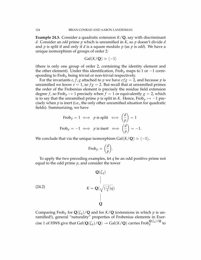
124 BRIAN CONRAD AND AARON LANDESMAN
Example 24.3. Consider a quadratic extension K/Q, say with discriminantd. Consider an odd prime p which is unramified in K, so p doesn’t divide dand p is split if and only if d is a square modulo p (as p is odd). We have aunique isomorphism of groups of order 2:
Gal(K/Q) ' 〈−1〉
(there is only one group of order 2, containing the identity element andthe other element). Under this identification, Frobp maps to 1 or −1 corre-sponding to Frobp being trivial or non-trivial respectively.
For the invariants e, f , g attached to p we have e f g = 2, and because p isunramified we know e = 1, so f g = 2. But recall that at unramified primesthe order of the Frobenius element is precisely the residue field extensiondegree f , so Frobp 7→ 1 precisely when f = 1 or equivalently g = 2, whichis to say that the unramified prime p is split in K. Hence, Frobp 7→ −1 pre-cisely when p is inert (i.e., the only other unramified situation for quadraticfields). Summarizing, we have
Frobp = 1 ⇐⇒ p is split ⇐⇒(
dp
)= 1
Frobp = −1 ⇐⇒ p is inert ⇐⇒(
dp
)= −1.
We conclude that via the unique isomorphism Gal(K/Q) ' 〈−1〉,
Frobp =
(dp
).
To apply the two preceding examples, let q be an odd positive prime notequal to the odd prime p, and consider the tower
(24.2)
Q(ζq)
K = Q(√(−1
q )q)
Q
Comparing Frobp for Q(ζq)/Q and for K/Q (extensions in which p is un-ramified!), general “naturality” properties of Frobenius elements in Exer-
cise 1 of HW8 give that Gal(Q(ζq)/Q) � Gal(K/Q) carries FrobQ(ζq)/Qp to

MATH 154. ALGEBRAIC NUMBER THEORY 125
FrobK/Qp , so via the identification of the two maps
(24.3)
Gal(Q(ζq)/Q) Gal(K/Q)
(Z/qZ)× 〈−1〉
we have that p mod q 7→ ((−1|q)q|p). But the cyclic group (Z/qZ)× hasonly one order-2 quotient, namely by the index-2 subgroup of squares mod-ulo q, so it follows that ((−1|q)q|p) = (p|q). This is exactly quadratic reci-procity! (See [Samuel, Ch. VI, §5] for full details, including a related argu-ment using Q(ζ8) to deduce the supplementary law for (2|p).)Remark 24.4. For p unramified in a Galois extension K′/K, Fr(p′|p) has or-der f , so since p is totally split if and only if (e = 1 and) f = 1, it is totallysplit if and only if Fr(p′|p) = 1 for some (equivalently, all) p′ over p.
For the rest of the course, we’ll discuss the proofs and applications of twofundamental finiteness theorems. To formulate the first one, we need somenotation. For a number field K, the class group Cl(K) denotes the groupCl(OK) studied in Homeworks 6 and 7: this is the group of fractional idealsmodulo principal ideals. We call hK := # Cl(K) the class number of K whenit is finite. Note that hK = 1 if and only if OK is a PID. Since a Dedekinddomain is a PID if and only if it is a UFD, this is also equivalent to OK beinga UFD. The first big finiteness theorem is:Theorem 24.5. Any number field has finite class number.
To state the second big finiteness theorem, the Dirichlet Unit Theorem, weneed some more notation. For K a number field, we let r1 denote the num-ber of embeddings K → R and let 2r2 denote the number of embeddingsK → C which do not factor through R (these come in conjugate pairs, sincecomposing with complex conjugation changes any non-real embedding). Weemphasize that these are counts of maps, and not of the image subfields un-der such maps. For example, if K/Q is Galois then all such embeddingshave the same image but there are [K : Q] distinct embeddings (since C isalgebraically closed).
In general, since C is algebraically closed (so the minimal polynomialover Q of a primitive element of K splits completely over C), we have
r1 + 2r2 = #{K → C} = [K : Q] =: n.
Theorem 24.6 (Dirichlet Unit Theorem). For K a number field, O×K is a finitelygenerated group of rank r1 + r2 − 1. Equivalently,
O×K ' µ× Zr1+r2−1

126 BRIAN CONRAD AND AARON LANDESMAN
for µ the (finite!) group of roots of unity in K.
Remark 24.7. In Exercise 4 in Homework 7, for a finite set
S = {p1, . . . , pm}
of primes of K (notation not to be confused with a multiplicative set for lo-calization) we defined the ring OK,S of S-integers of K (whose set of maximalideals is that of OK with S removed) and saw that
Cl(OK,S) = Cl(OK)/〈[pi]〉i.
Thus, Cl(OK,S) is trivial if we choose the pi to generate Cl(OK), as we canalways do since each of the finitely many elements of Cl(OK) is representedby a nonzero ideal of OK that in turn is a product of finitely many primes.(It is true that every element of Cl(OK) is the class of a prime ideal on thenose, but that is beyond the level of the course.) In this case, OK,S is a UFD.
It was seen in Homework 7 that for any such S there exists a ∈ OK − {0}so that OK,S = OK[1/a], so OK[1/a] is a UFD for some a. This latter propertyis very specific to the Dedekind domains OK that arise from number fields.For instance, in contrast the Dedekind domain
A := C[x, y]/(y2 − (x3 − x))
has uncountable class group and A[1/a] is not a UFD for any a ∈ A− {0};the proof involves the theory of elliptic curves. Similarly, for the Dedekinddomain B = Q[x, y]/(y2 − (x3 − 36x)), deeper input from the theory ofelliptic curves shows Cl(B) = (Z/2Z)2⊕ Z (countably infinite!) and B[1/b]is not a UFD for any b ∈ B− {0}.
The proof of finiteness of the class group will be effective, in the sense thatit gives explicit bounds on where to search to find generators. However, theproof of Dirichlet’s Unit Theorem uses a compactness argument and is noteffective (in a suitable sense). To illustrate the more subtle nature of findingunits, let’s first see what the Unit Theorem is saying for some small valuesof the rank r1 + r2 − 1. Since r1 + 2r2 = n, it follows that
r1 + r2 − 1 = 0 ⇐⇒ K is either imaginary quadratic (r2 = 1, r1 = 0)
or K = Q (r2 = 0, r1 = 1).
Likewise we have r1 + r2 − 1 = 1 if and only if either
r1 = 2, r2 = 0 (i.e., real quadratic),r1 = 0, r2 = 1 (i.e., quartic extensions with no real embedding),r1 = 1, r2 = 1 (i.e., cubic extensions with one real embedding).

MATH 154. ALGEBRAIC NUMBER THEORY 127
Let’s consider the real quadratic case. For real quadratic K the only rootsof unity are ±1 (as R doesn’t contain higher-order roots of unity), so
O×K = 〈−1〉 × εZK,
where εK is a fundamental unit, meaning a generator of the unit group mod-ulo the torsion subgroup {±1}. There are 4 fundamental units: ±εK,±1/εK,so if we fix an embedding j : K ↪→ R then there is exactly one fundamentalunit in each of the 4 connected components of R−{0,±1} (transitively per-muted via iterating the operations x 7→ 1/x and x 7→ −x). The unique onein (1, ∞) is often called “the” fundamental unit of K (relative to j).
Example 24.8. The variation of the fundamental unit is quite erratic as wevary the real quadratic field K, as illustrated with the following 3 cases:
K εK > 1Q(√
381) 1015 + 52√
381Q(√
382) 164998439999 + 8442054600√
382Q(√
383) 18768 + 959√
383
TABLE 1. Variation of εK for some real quadratic fields
Example 24.9. For a higher-rank illustration of the Unit Theorem, considerK = Q(ζp) for p > 3. We have r1 = 0, so 2r2 = p− 1 and hence r1 + r2− 1 =(p− 3)/2 > 0. Thus,
Z[ζp]× = µ2p × 〈ε1, . . . , ε(p−3)/2〉
for some multiplicatively independent ε1, . . . , ε(p−3)/2. In general, it is quitedifficult to find such ε j’s, but one can give an explicit multiplicatively inde-pendent subgroup of finite index (called the cyclotomic units) as follows.
For 2 ≤ j ≤ p− 2 (so p− 3 values of j) we define
uj = (ζ1/2p )1−j ·
1− ζjp
1− ζp
(note that ζ1/2p makes sense unambiguously since one can uniquely divide
by 2 in a finite abelian group of odd order). The root of unity multiplier inthe definition of uj is rigged to ensure that up−j = −uj (as one may checkwithout difficulty). These multiplicative dependence relations (i.e., up−j/ujis 2-torsion for all j) imply that the group of uj’s has rank at most (p− 3)/2(generated by uj’s for 2 ≤ j ≤ (p− 1)/2).
128 BRIAN CONRAD AND AARON LANDESMAN
For explicit small p one can use techniques from the proof of the UnitTheorem to show that the rank of the group of cyclotomic units is exactly(p− 3)/2 (so this group has finite index in Z[ζp]×), but to prove the same forall p requires a theoretical argument ultimately relying on analytic input viaL-functions. It turns out that the finite index of the group of cyclotomic unitsinside Z[ζp]×/µ2p is exactly the class number hQ(ζp)+ of the maximal realsubfield Q(ζp)+ = Q(ζp + ζ−1
p ) of Q(ζp), a fact that was first discovered inthe course of Kummer’s work on Fermat’s Last Theorem.
In a handout “Diophantine Applications of Class Groups” we give someapplications of class group computations to two types of arithmetic ques-tions. Let us survey the highlights of one of those here:
Example 24.10. Consider y2 = x3 − 51. It can be shown that this has so-lutions in Z/mZ for all m > 1 and that it has infinitely many Q-solutions(one of which is (1375/9, 50986/27)). However, there are no solutions overZ! This is interesting because it cannot be proven by congruential methods(due to the existence of solutions modulo m for all m > 1).
As in the first lecture of the course, one begins by rewriting it as
x3 = y2 + 51 = (y +√−51)(y−
√−51).
Now a new difficulty emerges: one has hQ(√−51) > 1, so the ring of integers
Z[√−51] is not a UFD. Thus, the analogue of the step showing that certain
quantities are cubes seems doomed.But a miracle happens: it turns out that 3 - hQ(
√−51), so there is no non-
trivial 3-torsion in the class group and hence any nonzero (potentially non-principal) ideal of Z[
√−51] whose cube is principal must itself be principal.
This allows one to push through a version of the method from the first dayof class “as if” Z[
√−51] were a UFD! The key in the end is that a non-trivial
class number is nonetheless coprime to 3, a property that cannot be seen viacongruential considerations in the ring of integers.
(In Kummer’s work on Fermat’s Last Theorem for exponent p, he madedecisive progress in the cases for which p - hQ(ζp), called “regular” primes.In these cases, to battle with unit issues it was crucial that Kummer hadthe explicit group of cyclotomic units whose index is hQ(ζp)+ . The subtleinterplay of units and class groups is a pervasive issue in number theory.)
25. COMPUTING SOME CLASS GROUPS
We wish to state a more precise version of the finiteness of class numbers(Theorem 24.5). This requires some notation:

MATH 154. ALGEBRAIC NUMBER THEORY 129
Definition 25.1. Let K be a number field and n := [K : Q]. Let r1 be thenumber of real embeddings, and 2r2 be the number of non-real complexembeddings, so r1 + 2r2 = n. Define the Minkowski constant for K to be
λK :=n!nn (4/π)r2
√|disc K|
Here is the precise version of finiteness:
Theorem 25.2. Let K be a number field. Each element of Cl(K) is the ideal class[a] of a nonzero ideal a ⊂ OK such that
Na ≤ λK.
Note that there are only finitely many a = ∏i prii with (Npi)
ri ≤ λK for alli since this latter inequality bounds the possibilities for the rational primepi | Npi over which pi lies (so there are only finitely many possibilities foreach pi), and also bounds the possibilities for ri since pri
i ≤ λK. This yields:
Corollary 25.3. For K a number field, Cl(K) is generated by the classes [p] for thefinitely many primes p over the finitely many primes p ∈ Z+ such that p ≤ λK.
Let’s now see some consequences of the preceding more precise versionsof the finiteness result.
Example 25.4. If λK < 2 then hK = 1 since there are no p’s satisfying Np ≤λK and hence the only possibility for a in the preceding discussion is theunit ideal (so Cl(K) = {1}, or equivalently OK is a UFD).
Let’s see what this yields when K = Q(√
d) for squarefree d ∈ Z− {0, 1}.(1) If d > 0, then n = 2, r1 = 2, r2 = 0, so
λK =
{12
√d if d ≡ 1 mod 4,√
d if d ≡ 2, 3 mod 4.
(2) If d < 0, then n = 2, r1 = 0, r2 = 1. We then obtain
λK =
{2π
√|d| if d ≡ 1 mod 4,
4π
√|d| if d ≡ 2, 3 mod 4.
Thus, we have λK < 2 (and hence hK = 1) precisely for
d = 2, 3, 5, 13,−1,−2,−3,−7.
In fact, these are all norm-Euclidean, so such cases are not so impressive fortriviality of the class number (though admittedly the preceding approachtreats all of them by a single slick method, without needing to battle withdifferent norm formulas in many cases).
130 BRIAN CONRAD AND AARON LANDESMAN
But hK = 1 in many more cases by using more refined techniques to com-pute class groups as we shall begin to illustrate later today. For example,
hK = 1 if d = 17, 19, 21, 29, 33,−11
but λK > 2 in all of these cases. The case K = Q(√−19) also satisfies hK = 1
and it can be proved that OK is not Euclidean (i.e., it has no possible normfunction!).
For the rest of today, we answer the following question via concrete ex-amples:
Question 25.5. When λK ≥ 2, how do we find relations among the idealclasses [p] for primes p|p with p ≤ λK?
We shall focus on some imaginary quadratic cases, taking up the harderreal quadratic case next time (the extra difficulty due to units not of finiteorder, as we shall see).
Example 25.6. Consider K = Q(√−14). We will show
Cl(K) ' Z/4Z.
Let’s first work out the Minkowski constant. We have n = 2, r1 = 0, r2 =1, disc K = −56, so approximately
λK ∼ 4.764 . . .
Therefore, Cl(K) is generated by [p] for p over 2 and 3, so we should factorthe ideals (2) and (3) into primes and then try to find as many relations aswe can among the ideal classes of those prime factors. Recall that
OK = Z[√−14] = Z[x]/(x2 + 14).
Thus, by Dedekind’s method, to find the primes above 2 and 3, we factorx2 + 14 mod p for p = 2 and 3. We get
(2) = p22,
(3) = p3p′3,
for p2 the unique prime above 2 and p3, p′3 the two distinct primes above 3.We conclude that the class group Cl(K) is generated by [p2], [p3] because[p′3] = [p3]
−1 (as the product p3p′3 is principal). Also, [p2]
2 = 1.We’d like to determine if [p2] has order 2 or order 1; we just saw that
its order divides 2. Since there is only one prime p2 over 2 and its normis 2, the principality of p2 is equivalent to finding α ∈ OK with |Nα| = 2.Also, Nα ≥ 0 for all α ∈ OK since K is imaginary quadratic. Explicitly,if α = u + v
√−14 with u, v ∈ Z then 2 = Nα = u2 + 14v2, but this is
impossible, so [p2] has order exactly 2.

MATH 154. ALGEBRAIC NUMBER THEORY 131
What can we do about [p3]? The key idea comes now: if we can find anelement of norm 6 then its principal ideal would yield a relation in the classgroup between the classes of p2 and either p3 or p′3 (with [p′3] = [p3]
−1), andin general if we can find an element α for which the only prime factors of itsnorm are 2 and 3 then factoring (α) will give us a relation between p2 andp3 in the class group. We now state this more precisely.
Norm technique. For K = Q(θ), with θ ∈ OK, and elements α := ∑n−1i=0 ciθ
i
with ci ∈ Z we compute
Nα = N(n−1
∑i=0
ciθi) ∈ Z.
The principal ideal (α) is a product of primes p over the primes p | N(α),yielding relations among such [p]’s in Cl(K). Hence, if we can find some αfor which the prime factors of N(α) all satisfy p ≤ λK then we get relationsin the class group among some primes p over such p.
To see this technique in our example K = Q(√−14), consider
N(m +√−14) = m2 + 14
for various m ∈ Z. We have N(1 +√−14) = 15 and N(2 +
√−14) = 18 =
2 · 32. Therefore, for some prime p5 above 5 we have
(1 +√−14) = p5 · p3 or p5 · p′3
We cannot yet distinguish if p3 or p′3 is a factor because we have not yetstated which prime above 3 is p3. Similarly, we have that (2+
√−14) factors
as one among the possibilities
p2p23, p2p3p
′3, p2(p
′3)
2.
We can rule out the second case since p3p′3 = (3) and 3 - (2 +
√−14) in
Z[√−14]. Thus, swapping p3 and p′3 if necessary, we may arrange that
(2 +√−14) = p2p
23,
so
[p3]2 = [p2]
−1
where [p2] has order 2.Therefore, [p3] has order 4: its order divides 4, but its order does not
divide 2 because its square is inverse to the element [p2] that is nontrivial(even with order exactly 2). This implies
Cl(K) = 〈[p3]〉 ' Z/4Z.

132 BRIAN CONRAD AND AARON LANDESMAN
Example 25.7. For K = Q(√−30) we have n = 2, r1 = 0, r2 = 1, disc K =
−120, so
λK ∼ 6.97 . . .
We therefore need to study the primes p over (2), (3), and (5). We claimCl(K) = Z/2Z× Z/2Z. Using that 2, 3, and 5 are all ramified, one then hasthree generators which are all 2-torsion. By norm considerations as above,these 2-torsion ideal classes are all non-trivial. In Homework 9, one finds afurther relation among them and shows it is “the only relation”.
Example 25.8. Consider K = Q(√−65). Since −65 ≡ 3 mod 4, we have
OK = Z[√−65].
We claim
Cl(K) = (Z/4Z)× (Z/2Z).
Computing the Minkowski constant, we get
λK =4π
√65 ∼ 10.26,
so we need to look at the factors of (2), (3), (5) and (7) in Z[√−65].
By factoring x2 + 65 mod p for p = 2, 3, 5, 7, we get
(2) = p22
(3) = p3p′3
(5) = p25
(7) = p7.
We therefore see the class group is generated by the classes of p2, p3, p5, sincethe class of p7 is trivial and [p′3] = [p3]
−1. We further see p2 and p5 are 2-torsion in the class group. In fact, all of p2, p3, p5 are not principal becausetheir norms are 2, 3, and 5 and one cannot write any of 2, 3, or 5 in the formu2 + 65v2 for u, v ∈ Z.
This tells us that [p2] and [p5] both have order exactly 2 in the class group.We now want to link [p3] to [p2] and [p5] using the norm technique from theprevious example. We seek an element whose norm only involves 2, 3, and5 as prime factors. To do this, we compute
N(a +√−65)
for various small a ∈ Z. (There is no particular reason that we have a coef-ficient 1 in front of
√−65; we are just playing around and trying different

MATH 154. ALGEBRAIC NUMBER THEORY 133
things.) That is, we hope to find some a2 + 65 with all prime factors in{2, 3, 5}.
Try a = 4 and a = 5: N(4 +√−65) = 81 = 34 and N(5 +
√−65) = 90 =
2 · 32 · 5. Therefore,
(4 +√−65) = p4
3 or p′43
using that 3 - (4+√−65) (to rule out any intervention by p3p
′3). Let’s relabel
p3 and p′3 if necessary so that (4 +√−65) = p4
3. Then
(5 +√−65) = p2p5p
′23
since we know it is a product of a prime above 2, a prime above 5, and twoprimes above 3 with the two primes above 3 equal to each other (i.e., p3and p′3 can’t both appear) because 3 - (5 +
√−65) and not both equal to p3
because p3 | (4 +√−65) yet 4 +
√−65 and 5 +
√−65 generate 1 (so their
associated principal ideals cannot have a common prime factor, such as p3).Therefore,
1 = [p2][p′3]
2[p5]
= [p2][p3]−2[p5].
This relation among the ideal classes of p2, p3, p5 allows us to drop [p5] fromthe list of generators: Cl(K) is generated by the element [p2] of order 2 andthe element [p3] of order dividing 4.
We claim [p3] has order exactly 4. We know its order is either 2 or 4 sincep3 is not principal. To rule out the possibility [p3]
2 = 1, suppose otherwise,so p2
3 = (α) for some α that must satisfy Nα = 9. If we write Nα = u2 + 65v2,we see that the only way this can happen is if u = ±3, v = 0, which wouldsay p2
3 = (α) = (3) = p3p′3, an absurdity (since p′3 6= p3). Therefore, we have
a surjection
Z/4Z× Z/2Z→ Cl(K)
with Z/4Z corresponding to the subgroup generated by [p3] and Z/2Z cor-responding to the subgroup generated [p2]. In particular, the class grouphas order dividing 8.
To show this surjective map is an isomorphism, we only need rule out thepossibility that the class group doesn’t have order 8, which is to say that itcoincides with its subgroup of order 4 generated by [p3]. In this latter casewe would have [p3]
2 = [p2] for order reasons, so we just need to rule outthis latter equality.
Suppose [p3]2 = [p2], so
[p2][p3]2 = [p3]
4 = 1.
134 BRIAN CONRAD AND AARON LANDESMAN
Therefore, we would obtain
p2p23 = (α)
for some α = u + v√−65 with u, v ∈ Z. But then
u2 + 65v2 = Nα = 18,
which is clearly impossible. Thus,
Cl(K) ' Z/4Z× Z/2Z
Next time, we’ll investigate a real quadratic example, in which case we’llhave to grapple with new difficulties involving units.
26. NORMS AND VOLUMES
An example of the class group of a real quadratic extension. Last time, weworked out a number of examples of class groups of imaginary quadraticfields. We’ll begin by working through an example of a real quadratic case.It will become apparent why this is harder when we encounter the plethoraof units in the associated ring of integers.
Example 26.1. Let’s compute Cl(K) for K = Q(√
82). We’ll show Cl(K) =Z/4Z. We have n = 2, r1 = 2, r2 = 0, disc(K) = 4 · 82, so
λK ∼ 9.055 . . .
The upshot is that the class group is generated by the classes [p] for primesp over 2, 3, 5, and 7.
Since OK = Z[√
82] = Z[x]/(x2 − 82), to factor pOK is the same as tofactor x2 − 82 ∈ Fp[x]. Thus, (2) = p2
2 and (3) = p3p′3 for primes p3 6= p′3.
Via quadratic reciprocity or by hand one can check that 82 is not a squaremodulo 5 and 7, so (5) and (7) are actually prime in OK. Therefore, Cl(K)is generated by [p2] (which is 2-torsion) and [p3] (the class of either of theprimes over 3).
Let’s now cross our fingers and hope we can find some nonzero elementin OK whose norm has as only 2 and/or 3 as its prime factors: we’ll compute
N(a +√
82) = a2 − 82
for some small integers a. Doing this, we eventually discover
N(10 +√
82) = 18 = 2 · 32.
This tells us
(10 +√
82) = p2 · p23

MATH 154. ALGEBRAIC NUMBER THEORY 135
after possibly switching p3 and p′3. Here we are using that 3 visibly does notdivide 10 +
√82 in OK = Z[
√82], so (10 +
√82) cannot have both p3 and p′3
as prime factors (as their product is (3)).Therefore,
[p3]2 = [p2]
−1 = [p2].
We conclude that [p3] generates the class group and is 4-torsion. To show[p3] has order exactly 4, it suffices to show that the ideal class [p3]
2 = [p2] isnontrivial; i.e., we are reduced to showing p2 is not principal.
So far, we have not encountered any difficulties in dealing with a realquadratic field instead of an imaginary quadratic field. Suppose p2 = (α)
for some α ∈ OK = Z[√
82]; we seek a contradiction. We can write α =u + v
√82 for some u, v ∈ Z. The equality p2 = (α), implies |NK/Q(α)| =
Np2 = 2 so u2− 82v2 = NK/Q(α) = ±2. Conversely, if NK/Q(α) = ±2, then(α) = p2 since p2 is the unique prime over (2).
Hence, our task of showing [p2] 6= 1 is equivalent to showing
x2 − 82y2 = ±2(26.1)
has no solutions in Z. The huge difference in this real quadratic case is thatto rule out integral solutions to such a “norm equation” we can no longersimply do a quick finite check as in the imaginary quadratic case.
In O×K , we have a fundamental unit given by
ε = 9 +√
82.(26.2)
What really matters initially is that N(ε) = −1, so after potentially multi-plying by ε we see that if we had a solution to (26.1) for one of the signs onthe right side then we get a solution for the other sign too. Hence, it doesn’tactually matter whether we consider 2 or −2 on the right side.
To appreciate the subtlety involved in proving the absence of Z-solutions,we observe two features of the conic (26.2) with +2 on the right. Firstly, ithas infinitely many Q-points, one of which is (10/3, 1/3). Moreover, thisconic even has points modm for all m ≥ 1 (this requires some work, but isultimately some effort with congruential algebra and doesn’t involve any-thing very deep, though handling m divisible by high powers of 2 or 41 doesentail some additional thought); e.g., for m = 41 we have 172 ≡ 2 mod 41and −1 is a square modulo 41, so −2 is also a square modulo 41.
The upshot is that we cannot rule out Z-solutions just by congruence rea-sons, so the absence of such solutions is not an entirely “elementary” asser-tion. On Exercise 5 of Homework 9 you will show (26.1) has no Z-solutions.A key input in the argument, going beyond congruential information, isthat ε is a fundamental unit satisfying N(ε) = −1, due to which the units of

136 BRIAN CONRAD AND AARON LANDESMAN
norm 1 are up to a sign precisely the squares of units. One builds on that toshow that if there exists a Z-solution then one of ±2 is a square in Q(
√82),
which is absurd.
The geometry of numbers. Finiteness of class groups and finite generationof unit groups were understood by the 1880’s, but in 1896 Minkowski cameup with a way to establish such results via consideration of lattices in Eu-clidean spaces attached to number fields. His method, called “geometry ofnumbers”, has applications to the arithmetic of quadratic forms and manyother problems in number theory.
We shall turn the questions of finiteness of the class group and finite gen-eration of units into one of finding nonzero vectors of lattices contained inspecific bounded regions in a Euclidean space. To achieve this, we shallshow the following reformulation of the refined finiteness of class numbers:
Theorem 26.2. For any nonzero ideal b ⊂ OK, there is some β ∈ b− {0} suchthat
|NK/Q(β)| ≤ λK · Nb.
Let’s see why this implies Theorem 25.2.
Proof. The fractional ideal a := βb−1 lies inside OK since β ∈ b (think backto how b−1 is defined), so a is an ordinary nonzero ideal of OK. We have
[a] = [b]−1
and Na = |NK/Qβ|Nb−1 ≤ λK. The upshot is that [b]−1 has an integral idealrepresentative with norm at most λK. However, every element of Cl(K) hasthis form, since b is just an integral representative of the inverse class. �
We next aim to give a geometric interpretation of norms in terms of vol-umes of parallelotopes in some RN. Which RN do we take?
The time has come to consider all embeddings of a number field into Cat once (e.g., for a real quadratic field, it will be essential to treat both realembeddings on an equal footing, and not prefer one over the other). Thekey geometric tool is the following map:
θK : K → Rr1 × Cr2
x 7→ (σ1(x), . . . , σr1(x), σr1+1, . . . , σr1+r2(x))
where we identify Rr1 ×Cr2 with Rn for n = r1 + 2r2 via identifying C withR⊕ R · i; here σ1, . . . , σr1 : K → R are the real embeddings and
σj, σj : K ⇒ C
for r1 + 1 ≤ j ≤ r1 + r2 is the set of conjugate pairs of non-real embeddings.

MATH 154. ALGEBRAIC NUMBER THEORY 137
Lemma 26.3. For any nonzero ideal b ⊂ OK the image θK(b) ⊂ Rn is a lattice(i.e., the Z-span of a R-basis).
Proof. Any Z-basis of b is a Q-basis of K, so it is enough to show that if{e1, . . . , en} is any Q-basis of K then the n vectors {θK(ej)}1≤j≤n is an R-linearly independent set in Rn.
To show this, it is the same to show that the n× n real matrix
M =
θK(e1)...
θK(en)
has nonzero determinant. We will establish this using column operations,actually working with |det(M)| and regarding M as a matrix with its n2
entries in C rather than just in R (so we may applying column operationsinvolving scaling against elements of C× such as ±i).
More explicitly, writing <(z) and =(z) to denote the real and imaginaryparts of z ∈ C, M is given as:σ1(e1) . . . σr1(e1) <σr1+1(e1) =σr1+1(e1) . . . <σr1+r2(e1) =σr1+r2(e1)
... . . . ......
... . . . ......
σ1(en) . . . σr1(en) <σr1+1(en) =σr1+1(en) . . . <σr1+r2(en) =σr1+r2(en)
The rightmost 2r2 columns come in pairs <σj and =σj, so for such r1 + 1 ≤j ≤ r1 + r2 if we multiply the column of =σj’s by −i (which has no effect on|det(M)|) and subtract this from the column of <σj’s then we turn the <σj-column into σj. Next, doubling each −i=σj-column is counteracted by mul-tiplying the determinant by 2−r2 . Adding the σj-column to the −2i=(σj)-column yields σj in place of −2i=σj. Therefore, we have arrived at the ma-trix in Matn(C) given byσ1(e1) . . . σr1(e1) σr1+1(e1) σr1+1(e1) . . . σr1+r2(e1) σr1+r2(e1)
... . . . ......
... . . . ......
σ1(en) . . . σr1(en) σr1+1(en) σr1+1(en) . . . σr1+r2(en) σr1+r2(en)
In other words, this is the matrix (σ(em)) whose entries are indexed by pairs(σ, m) for all embeddings σ : K → C and 1 ≤ m ≤ n. Our task is reduced toshowing that this latter matrix has nonzero determinant.
This final non-vanishing property is independent of the choice of Q-basis{ej} of K since it is easy to check that if we applying an invertible Q-linearchange of basis to {ej} then this final matrix is changed via multiplicationagainst an invertible n × n matrix with rational entries. Thus, it is nowenough to consider the matrix (σ(em))(σ,m) for one Q-basis {ej} of K. Weconsider a power basis! That is, for α ∈ K a primitive element over Q, take

138 BRIAN CONRAD AND AARON LANDESMAN
{ej} to be {1, α, . . . , αn−1}. Then our matrix is (σ(αm)), which is precisely thematrix that came up in the proof of the non-vanishing of the discriminantof K: this is a van der Monde matrix whose determinant is nonzero sinceσ(α) 6= τ(α) for any σ 6= τ (as Q(α) = K). �
27. VOLUME CALCULATIONS
Application of K → Rr1 ×Cr2 to video games. There is a video game calledLucy and Lily by Rich Schwartz, a math professor at Brown; it is on his web-page at Brown, and he wrote an article about it for the American MathematicalMonthly (also on his webpage).
Take K = Q(ζ) for a primitive 5th root of unity ζ. We consider two pen-tagons in their own copies of C, with center at the origin and vertices at the5th roots of unity in C; call these pentagons Lucy and Lily (the names ofRich Schwartz’ children). Each pentagon is dissected into 5 equal sectors asusual (sector edges joining the vertices to the center), colored with a com-mon set of 5 colors. The coloring order in the counterclockwise direction ofLily is related to that of Lucy by doubling the angles (note that 2 generates(Z/5Z)×). Combining this information amounts to considering
θK : OK = Z[ζ]→ C× C
defined by ζ 7→ (ζ5, ζ25) for ζ5 := e2πi/5.
The pentagons move by flipping across an exterior edge, and whateveris done in one plane happens in the other via flipping through the exterioredge of the same color (so geometric effects in the two planes are different,due to the angle-doubling on colored sectors). The game begins by clos-ing your eyes while the computer does many flips, and the challenge uponopening your eyes is to move Lucy back to 0 through exterior edge flips.This is impossible to win using just Lucy because the discrete θK(Z[ζ]) ⊂ C2
has dense image under projection to either factor C (so the set of centers oflegal positions of the pentagon is dense!); a later handout will prove density.
The “winning strategy” (explained at length in the AMM article) exploitsthe discreteness of OK in C2 = R4 to overcome the density of the image ofOK in each copy of C: one first moves Lucy as efficiently as possible towardsthe origin via exterior edge flips while Lily makes the “same” flips (basedon colors) but moves quite differently. The distance loss by Lily winds upbeing less than the gain made by Lucy, and so if we then switch to movingLily as efficiently as possible towards the origin we entail some loss for Lucyby it is not as bad as the gain by Lily. Then go back to efficient moves forLucy towards the origin, etc. The linked motion corresponds to makingprogress towards (0, 0) ∈ C2 in the lattice θK(OK) as measured by distancein R4, so by the discreteness of θK(OK) we eventually win (i.e., reach 0 ∈ C)!

MATH 154. ALGEBRAIC NUMBER THEORY 139
Remark 27.1. On the same website is a “√
2-game” with boats hopping dis-tances of 1 or
√2 in R to illustrate the phenomenon with K = Q(
√2)→ R2:
one sees 2-dimensional discreteness and 1-dimensional density, and whythe strategy of moving optimally in alternating “parallel worlds” works.
Geometric meaning of determinant.
Lemma 27.2. Let Λ ⊂ Rn be a lattice, and let v := {vi} be an ordered Z-basis ofΛ. For the parallelotope Pv := {∑i tivi | 0 ≤ ti ≤ 1}, Vol(Pv) is independent of vand is given by the n× n absolute determinants:
(27.1) Vol Pv =
∣∣∣∣∣∣det
v1...
vn
∣∣∣∣∣∣ = ∣∣det(v1 · · · vn
)∣∣(where both matrices inside the determinants are n× n).
FIGURE 1. Both v = {v1, v2} and v′ = {2v1 − v2,−3v1 + v2}have the same Z-span, and Pv and Pv′ have the same area.

140 BRIAN CONRAD AND AARON LANDESMAN
Before proving the lemma, we make some observations. From a geomet-ric viewpoint the independence of v may be a bit surprising. For examplewith n = 2, v′ = {2v1− v2,−3v1 + v2} is also a Z-basis of Zv1⊕Zv2 because
det(
2 −3−1 1
)= −1 ∈ Z×
(so the inverse is also an integer matrix), yet the geometry of the parallelo-grams Pv′ and Pv are very different (but areas agree), as shown in Figure 1.
Also, the real explanation for Pv having volume independent of v is thatthe compact coset space Rn/Λ that is intrinsic to Λ (i.e., it doesn’t involvea choice of v) inherits a natural measure from the one on Rn relative towhich its volume is that of every Pv (informally, Pv → Rn/Λ is a measure-preserving isomorphism “away from the measure-zero boundary”). How-ever, we don’t want to digress into a discussion of measures on coset spaces,so we opt for the perspective of Pv ⊂ Rn that is sufficient for our needs.
Now we take up the proof of the lemma:
Proof. By definition Pv is the image of [0, 1]n under the invertible linear map
T : Rn → Rn
corresponding to the n× n matrix(v1 · · · vn
)Therefore,
Vol(Pv) = |det T| ·Vol([0, 1]n),
which is the right side of (27.1).For independence of v, if v′ = {v′1, . . . , v′n} with v′j = ∑i aijvi another
ordered Z-basis of Λ then the integer matrix (aij) has inverse matrix that isalso an integer matrix (why?) and hence its determinant belongs to Z× ={±1}. But it is elementary to check (work it out for n = 2 first) that(
v′1 · · · v′n)=(v1 · · · vn
)· (aij)
as n× n matrices. Applying |det(·)| to both sides gives the result. �
Definition 27.3. We write VolΛ to denote Vol(Pv) for any ordered Z-basis vof Λ.
To apply the preceding lemma in the proof of finiteness of the class num-ber, let’s recall that we have previously reduced the finiteness to the follow-ing:

MATH 154. ALGEBRAIC NUMBER THEORY 141
Goal 27.4. For a nonzero ideal b ⊂ OK, we seek β ∈ b− {0} so that
|NK/Qβ| ≤ λK · Nb,
where
λK =n!
nn (4/π)r2
√|disc K|.
We need the following result to reinterpret our goal in terms of volumesattached to lattices:
Theorem 27.5. For a nonzero integral ideal b ⊂ KθK−→ Rr1 × Cr2 = Rn, we have
Volb := VolθK(b) = 2−r2
√|disc K| · Nb.
For example, in the above notation, we have
VolθK(OK) = 2−r2
√|disc K|.
Here is an explicit example:
Example 27.6. Take K = Q(α) with α2 = 3. Let’s define the embeddingsσi : K → R by σ1(α) =
√3 and σ2(α) = −
√3. Then OK = Z[α] and
θK(Z[α]) = {θK(a + bα) = (a + b√
3, a− b√
3) | a, b ∈ Z}
is the Z-span of θK(1) = (1, 1) and θK(α) = (√
3,−√
3). In other words,
(a + b√
3, a− b√
3) = a · (1, 1) + b · (√
3,−√
3)
is the lattice spanned over Z by θK(1), θK(α). Its associated volume (“area”)is ∣∣∣∣det
(1√
31 −
√3
)∣∣∣∣ = 2√
3 =√
12.
as desired. Similarly, for the ideal b = (1 + α) with norm |NK/Q(1 + α)| =| − 2| = 2 we have
θK(b) = {θK((1 + α) · (a + bα)) | a, b ∈ Z}= {((1 +
√3)(a + b
√3), (1−
√3)(a− b
√3)) | a, b ∈ Z}
= {a(1 +√
3, 1−√
3) + b(3 +√
3, 3−√
3) | a, b ∈ Z},so
Volb =∣∣∣∣det
(1 +√
3 3 +√
31−√
3 d−√
3
)∣∣∣∣ = 2√
12,
consistent with the fact that we saw Nb = 2.

142 BRIAN CONRAD AND AARON LANDESMAN
The proof of the general formula for Volb is given in the handout “VolumeAttached to an Ideal”. Here, we’ll explain why
Volb = Nb ·VolOK ;
the computation VolOK = 2−r2√|disc K| as given in that handout is essen-
tially a more refined version of what we did last time where we performeda linear transformation to turn the matrix for our embedding θK : K → Rn
into a van der Monde matrix related to a discriminant.Since Nb = [OK : b], the desired relation between Volb and VolOK is a
special case of the more general claim for any pair of lattices Λ′ ⊂ Λ in Rn
that
VolΛ′ = [Λ : Λ′] ·VolΛ .
By the structure theorem for modules over a PID, we can always choose Z-bases of the two lattices so that the Z-basis of Λ’ is given by multiples of aZ-basis of Λ:
Λ = ⊕Zvi, Λ′ = ⊕Z(civi)
for some ci ∈ Z − {0}. Thus, [Λ : Λ′] = ∏i |ci|, and for v′ = {civi} theparallelogram Pv′ is covered by ∏i |ci| translates of Pv that are “essentiallydisjoint” (from the viewpoint of volumes) in the sense that their pairwiseoverlaps are contained in hyperplanes (hence not contributing to volume):
Pv′ =⋃~r
(Pv + ∑ rjvj)
for varying ~r = (r1, . . . , rn) with 0 ≤ rj < |cj|. This implies Vol(Pv′) =(∏i |ci|) ·Vol(Pv), or equivalently VolΛ′ = [Λ′ : Λ]VolΛ as desired.
Now consider the diagram
(27.2)K Rr1 × Cr2
Q R
θK
|NK/Q| N
with N : Rr1 × Cr2 → R defined by
(~x,~z) 7→∏ |xi| ·∏ |zj|2.
It is left as an exercise to show this diagram commutes. (The main point isthat |z|2 = |z||z| impliesN ◦ θK : v 7→ ∏σ:K→C |σ(v)| = |∏σ:K→C σ(v)|withσ varying through all field embeddings K → C, including both members ofeach pair of conjugate non-real embeddings, so the commuting of the dia-gram reduces to the purely algebraic formula NK/Q(v) = ∏σ:K→C σ(v) for
MATH 154. ALGEBRAIC NUMBER THEORY 143
each v ∈ K, which in turn is proved via transitivity of field norms appliedto the tower K/Q(v)/Q.)
Using this, it suffices to prove the following result in which K has essen-tially disappeared (except for the values of r1 and r2 that acquire the statusof independent parameters in the formulation):
Theorem 27.7. For any r1, r2 ≥ 0 at least one of which is positive, n := r1 + 2r2,and any lattice L ⊂ Rr1 × Cr2 = Rn, we have
L ∩ {v ∈ Rn | N (v) ≤ n!nn (8/π)r2 VolL} 6= 0.
Theorem 26.2 follows from this general result for lattices applied to L =θK(b) due to the commutative diagram (27.2) and the general formula forVolb! We now prove Theorem 27.7:
Proof. Since r1 + 2r2 = n, for v = (~x,~z) ∈ Rr1 × Cr2 the arithmetic-meangeometric-mean inequality gives
N (v)1/n ≤ (∑i|xi|+ 2 ∑
j|zj|)/n.
Thus, it is enough to show
L ∩ {v ∈ Rn | ((∑i|xi|+ 2 ∑
j|zj|)/n)n ≤ n!
nn (8/π)r2 VolL} 6= 0
(note that the denominator nn on both sides of the inequality cancels out).To prove this latter assertion, we shall use the following volume compu-tation that is proved in [Samuel, Ch. IV, Appendix, pp. 66-67] via a cleverapplication of Fubini’s theorem and an induction on r1 and r2:
Lemma 27.8. For t > 0, the compact region
Xt := {(x, z) ∈ Rr1 × Cr2 | ∑i|xi|+ 2 ∑
j|zj| ≤ t}
satisfies
Vol(Xt) = 2r1(π/2)r2tn
n!.
Now, consider
D = {(x, z) ∈ Rr1 × Cr2 | ((∑i|xi|+ 2 ∑
j|zj|)/n)n ≤ n!
nn (8/π)r2 VolL}.
This is Xt0 of Lemma 27.8 for t0 satisfying
tn0 = n!(8/π)r2 VolL,

144 BRIAN CONRAD AND AARON LANDESMAN
so
Vol(Xt0) = 2r1(π/2)r2(8/π)r2 VolL
= 2r1+2r2 VolL
= 2n VolL .
Note that each Xt is compact, convex (i.e., it contains the line segmentjoining any two of its points), and symmetric around 0 (i.e., stable undernegation). Hence, we are reduced to the general result below that is trulyjust about lattices in Rn for any n > 0 and has nothing to do with K. �
Theorem 27.9 (Minkowski convex body theorem). If L ⊂ Rn is a lattice andD ⊂ Rn is compact, convex, and symmetric around 0 with
Vol(D) ≥ 2n VolL
then L ∩ D contains a nonzero element.
We will prove this next time. Note that D contains 0 (an obvious propertyfor D = Xt): D is non-empty due to positivity of Vol(D) and for d0 ∈ D thesymmetry forces −d0 ∈ D, so the convexity implies that the midpoint 0 ofthe segment joining d0 and −d0 belongs to D.
28. MINKOWSKI’S THEOREM AND APPLICATIONS
We have seen that finiteness of class numbers is reduced to Minkowski’sconvex body theorem stated at the end of last lecture (Theorem 27.9).
Remark 28.1. Kronecker’s original proof of finiteness of class numbers in1882 came before Minkowski’s invention of the geometry of numbers in1896 (and even before Minkowski earned his PhD in 1885). The proof (writ-ten in Latin) used a pigeonhole argument instead of volumes and got a con-stant λ′K depending on a choice of Z-basis of OK. Typically λ′K is much largerthan λK, and Minkowski’s geometric method has much wider significance(as we shall see).
Before proceeding with the general proof, let’s see the idea illustratedwhen n = 2. Pick a Z-basis {v, v′} for L. Define the “half-open” parallelo-gram
P := {tv + tv′ | − 1 ≤ t, t′ < 1},so Vol P = 4 VolL. We’ll treat the case Vol(D) > 4 VolL (and when treat-ing general n we’ll discuss a trick to handle the case of equality Vol(D) =2n VolL). The plane R2 is covered by disjoint translates Pα of the paral-lelogram P. Consider the overlaps D ∩ Pα. Only finitely many such arenonempty because D is bounded. Letting Dα ⊂ P be the translate of D ∩ Pα

MATH 154. ALGEBRAIC NUMBER THEORY 145
back into P, at least two such subsets Dα ⊂ P must have a non-empty over-lap because
∑α
Vol(Dα) = Vol(D) > 4 VolL = Vol(P).
Thus, for some α0 6= β0 there exists ξ ∈ D∩ Pα0 , ξ ′ ∈ D∩ Pβ0 that translateto the same point in P. These points ξ, ξ ′ ∈ D are distinct (since Pα’s arepairwise distinct) yet ξ − ξ ′ ∈ 2L, so 0 6= ξ−ξ ′
2 ∈ L. However, ξ ∈ D and−ξ ′ ∈ D (since D is symmetric), so by convexity the entire line segment ofpoints tξ + (1− t)(−ξ ′) for 0 ≤ t ≤ 1 belongs to D. Setting t = 1/2, themidpoint (1/2)(ξ − ξ ′) of the segment joining ξ and −ξ ′ belongs to D, butwe also saw that this belongs to L− {0}.Remark 28.2. It may seem that the full force of convexity is not needed inthis proof, since we only used that D is stable under passing to midpoints.However, via repeated bisections of a segment, stability under midpointsin general implies that a dense subset of the segment joining any two pointsof D is inside D. Thus, when D is closed it follows that the entire segmentbelongs to D, so stability under taking midpoints is equivalent to convex-ity. One might then ask where we use that D is closed. This is relevantin handling the case Vol(D) = 4 VolL which we didn’t discuss above butwill discuss in the treatment of general n below (and which also uses morecrucially that D is bounded).
Now we give the proof of Minkowski’s convex body theorem for all n.First, we explain how to reduce the case Vol D = 2n VolL to the case Vol D >2n VolL, using closedness of D. That is, assuming Theorem 27.9 holds for allcompact convex symmetric D′ with Vol D′ > 2n VolL we claim it also holds forcompact convex symmetric D satisfying Vol D = 2n VolL.
Pick some ε > 0 and consider the fattened region
Dε := (1 + ε) · Dthat is also compact, convex, and symmetric with volume
Vol Dε = (1 + ε)n Vol D > 2n VolL .
Thus, Dε ∩ L 6= {0} for all ε > 0. A priori, Dε ∩ L is finite since L is alattice Rn and Dε is bounded (this is easiest to see using coordinates relativeto a Z-basis of L, keeping in mind that boundedness in Rn is coordinate-independent: we just observe after a coordinate change to turn L into Zn
that a bounded subset of Rn has finite intersection with Zn).For ε′ < ε clearly Dε′ ∩ L ⊂ Dε ∩ L as finite sets, so for sufficiently small ε
all Dε ∩ L coincide. Thus, since these all contain a nonzero point of L, thereexists ` ∈ L − {0} belonging to ∩ε>0Dε. But this intersection that visibly

146 BRIAN CONRAD AND AARON LANDESMAN
contains D is contained in the closure D of D (writing ` = (1 + ε)dε for dε ∈D amounts to saying (1+ ε)−1` ∈ D, and these points for ε→ 0 converge to`, forcing ` ∈ D), yet D is closed by hypothesis, so this intersection is equalto D and hence D meets L− {0} as desired. (Note that we have used that Dis bounded and closed, or equivalently compact.)
We conclude that it suffices to treat the case Vol(D) > 2n VolL, which willproceed basically as in the case n = 2 that we settled already, up to somemore notation. Pick a Z-basis e = {ei} of L so Rn also has e as an R-basis:Rn = ⊕iRei. Define the “half-open” parallelotope
Pe := {∑i
tiei | − 1 ≤ ti < 1},
so Vol Pe = 2n VolL. Since
R = än∈Z
[2n− 1, 2n + 1) = än∈Z
([−1, 1) + 2n)
is the disjoint union of even translates of [−1, 1), by applying this alongeach coordinate direction for ⊕Rei = Rn we have
Rn = ä`∈2L
(Pe + `).
By boundedness of D, the overlap
D` := D ∩ (Pe + `)
of D with each 2L-translate of Pe is nonempty for only finitely many ` ∈2L. (This is most easily seen by working in the e-coordinate system of Rn,in terms of which 2L corresponds to 2Zn and Pe becomes [−1, 1)n.) Now,consider the translates
D′` := −`+ D` ⊂ Pe.
Since
∑`∈2L
Vol D′` = ∑`∈2L
Vol(D`)
= Vol(D)
> 2n VolL
= Vol Pe,
by volume reasons there exist distinct `1, `2 ∈ 2L so that
D′`1∩ D′`2
6= ∅.

MATH 154. ALGEBRAIC NUMBER THEORY 147
Therefore, there are points ξ1 ∈ D ∩ (Pe + `1) and ξ2 ∈ D ∩ (Pe + `2) suchthat −`1 + ξ1 = −`2 + ξ2. Note that ξ1 6= ξ2 since Pe + `1 and Pe + `2 aredisjoint (as `1 6= `2). But
0 6= ξ1 − ξ2
2∈ D
by convexity and symmetry (as in the case n = 2), and also
ξ1 − ξ2
2=
`1 − `2
2∈ 1
2(2L) = L.
Therefore, we have constructed a nonzero point (ξ1 − ξ2)/2 ∈ D ∩ L, asdesired.
Let’s now record some further applications of Minkowski’s convex bodytheorem, to illustrate its power. These results, unlike finiteness of class num-bers, were not known prior to Minkowski’s geometry of numbers.
Theorem 28.3 (Minkowski). If K 6= Q then |disc K| > 1. In particular, forK 6= Q there exist rational primes ramified in K.
Kronecker was led to initially conjecture this result via analogies betweenrings of integers and compact Riemann surfaces. See [Samuel, Theorem 1,p. 58] for a proof.
The next finiteness result is quite striking due to not imposing any con-straint on the degree over Q:
Theorem 28.4 (Hermite). For any B > 0 there are only finitely many numberfields K up to isomorphism with |disc K| ≤ B.
This result is proved in [Samuel, Theorem 3, p. 59]. As a complement, ifwe don’t constrain the discriminant but only its prime factors and we boundthe field degree then we get a finiteness result over any number field:
Theorem 28.5. For F a number field, S := {p1, . . . , pm} a finite set of primes ofF, and n > 1, the set of extensions K/F (up to isomorphism) of degree at most nramified at most over S is finite.
The proof of this result requires deeper input from ramification theory(such as higher ramification groups, a refinement of inertia groups), and isgiven in [Neukirch, Theorem 2.13, Ch III]. Ultimately, the idea of the proofis to use n and S to deduce a uniform bound on the discriminant of K overQ so that one can apply Hermite’s theorem.
Remark 28.6. Loosely speaking, the preceding theorem says that OF,S has“fundamental group” with strong finiteness properties (made precise usingGrothendieck’s theory of etale fundamental groups). This fits well into the

148 BRIAN CONRAD AND AARON LANDESMAN
analogy between rings of integers and compact Riemann surfaces, an anal-ogy that involves the theory of algebraic curves and often doesn’t help toprove things but can help in deciding what to try to prove!
Next time, we’ll prove the Dirichlet Unit Theorem which says that thegroup O×K is finitely generated with rank r1 + r2 − 1. Recall from HW5 Ex-ercise 1(ii) that the torsion subgroup
(O×K )tor = { roots of unity in K}
of O×K is finite. Thus, it is equivalent to show that the torsion-free groupO×K /(O×K )tor is finitely generated of rank r1 + r2 − 1. The key difficulty isto show the rank is as big as r1 + r2 − 1; we’ll see that finite generatednessand the rank being at most r1 + r2 − 1 are not so deep. The main task isto construct units not of finite order when r1 + r2 − 1 > 0 (i.e., when K isneither Q nor imaginary quadratic), which we will do using pigeonhole-type arguments via the geometry of numbers.
Example 28.7. For K = Q(21/4) we have r1 = 2 and r2 = 1 (since there areexactly two 4th roots of 2 in R and one conjugate pair of non-real 4th rootsof 2 in C), so Dirichlet’s Unit Theorem says rkZ O×K = 2. This is exhibited bythe explicit description O×K = 〈±1〉(1 + 21/4)Z · (1 +
√2)Z. (The only roots
of unity in K are ±1 since K admits a real embedding.) The proof we’ll giveof Dirichlet’s theorem is theoretical; to compute the unit group in a specificcase, one needs refinements of the theoretical methods (explained in bookson computational algebraic number theory).
29. THE UNIT THEOREM
Today we finally come to the proof of Dirichlet’s Unit Theorem, after wefirst discuss a few more illustrative examples. The proof will rest cruciallyon Minkowski’s geometry of numbers; Dirichlet’s original proof in 1846 (18years before Minkowski was born!) involved pigeonhole arguments insteadof the volume-theoretic method we will use. The modern algorithms for ac-tually computing generators of the unit group of an explicitly given numberfield rest on using “lattice reduction” techniques (for finding short vectorsin lattices) to make the method of proof below more explicit.
The idea for the original proof came to Dirichlet during a concert in theSistine Chapel in Rome. He had already proved special cases (such as forcubic fields), but the general case stumped him for some years. Minkowskiinvented the geometry of numbers 50 years later, in 1896.
Before proving the Unit Theorem, let’s see some more examples.

MATH 154. ALGEBRAIC NUMBER THEORY 149
Example 29.1. Suppose [K : Q] = 3. Since r1 > 0 (why?) and r1 + 2r2 = 3we have two possibilities for (r1, r2), so two possibilities for rk O×K :
rk O×K =
{2 if r1 = 3, r2 = 0;1 if r1 = 1, r2 = 1.
An instance of the first case is Q(α) with α3 − 3α + 1 = 0. For this, one hasO×K = 〈±1〉αZ(α + 1)Z. An instance of the second case is Q(21/3), for whichO×K = 〈±1〉(21/3 − 1)Z.
Example 29.2. Consider the biquadratic extension K = Q(√
2,√
3). Wehave r1 = 4 and r2 = 0, so rk O×K = 3. There are three quadratic subfields:Q(√
2), Q(√
3), Q(√
6). These give units 1 +√
2, 2 +√
3, 5− 2√
6 whichcan be shown to be multiplicatively independent by using the “log map”to be defined later. Thus, the group generated by these units is of finiteindex in O×K (and hence anything in O×K has a nontrivial power contained inthis subgroup). This subgroup really misses some infinite-order units. Forexample, it misses
√2−√
3 (with square 5− 2√
6) and (√
2 +√
6)/2 (withsquare 2 +
√3).
Example 29.3. Let p be an odd prime and K = Q(ζp). Inside K the subfieldK+ := Q(ζp + ζ−1
p ) equals the fixed field E of complex conjugation (as K+ iscertainly inside that “index-2” subfield E yet [K : K+] ≤ 2 since ζp is easilyseen to satisfy a quadratic relation over K+, so [K : K+] = 2 and K+ = E).
Thus, rK1 = 0, rK
2 = p−12 whereas rK+
1 = p−12 , rK+
2 = 0, so O×K+ ⊂ O×K hasfinite index. This generalizes with Q(ζp) replaced by any CM field (where“CM” stands for Complex Multiplication, an important notion in the theoryof abelian varieties).
To prove the Unit Theorem, we will first turn our multiplicative probleminto an additive problem via the so-called log map
L : O×K ⊂ K×θK−→ (R×)r1 × (C×)r2 `−→ Rr1+r2
where ` : (R×)r1 × (C×)r2 → Rr1+r2 is defined by
(x1, . . . , xr1 , z1, . . . , zr2) =: (x, z) 7→ (log |x1|, . . . , log |z1|2, . . . )
(output to be denoted below by the shorthand (log |x|, log |z|2)). The com-posite map L is therefore given by
L : O×K → Rr1+r2
u 7→ (log |σ(u)|, log |τ(u)|2)

150 BRIAN CONRAD AND AARON LANDESMAN
where σ varies through the r1 real embeddings and τ varies through ther2 non-real embeddings taken up to complex conjugation. Further, since|τ(u)|2 = |τ(u)| |τ(u)|, the sum of the coordinates of L (u) is preciselylog |NK/Q(u)| = log 1 = 0 (using that NK/Q(O
×K ) ⊂ {±1}).
Hence, we obtain
L (O×K ) ⊂ H := {t ∈ Rr1+r2 |r1+r2
∑j=1
tj = 0} ⊂ Rr1+r2
with dim H = r1 + r2− 1. No other linear dependence relation on the imageof L leaps to mind (beyond ∑ tj = 0), so we aim show it is a lattice in H.
Example 29.4. Let K = Q(α) with α2 = 2, so O×K = 〈±1〉(1 + α)Z. We haveθ : K → R2 via α 7→ (
√2,−√
2), so θ(a + bα) = (a + b√
2, a − b√
2) fora, b ∈ Q. Here, the log map ` : R× × R× → R2 is
(x, y) 7→ (log |x|, log |y|).The image θK(O
×K ) ⊂ R× × R× lies inside {|x||y| = 1} = {xy = ±1} ⊂
R2 as a discretely-placed set of points, and L (O×K ) is a lattice in the line{t1 + t2 = 0} ⊂ R2, as shown in Figure 2.
FIGURE 2. Picture showing θK(O×K ) ⊂ {|x||y| = 1} and ` car-
rying it into the line H = {t1 + t2 = 0} in R2.

MATH 154. ALGEBRAIC NUMBER THEORY 151
For later use, we define the norm-1 hypersurface
Σ := `−1(H) = {(x, z) ∈ Rr1 × Cr2 | ∏i|xi| ·∏
j|zj|2 = 1}
(equivalently, this is the set of points v ∈ Rr1 × Cr2 such that |N (v)| = 1).Note that ` carries Σ onto H. In the handout “Generalized Pell Equation”we use the log map to bound any possible Z-solution to x2 − dy2 = n forany given n ∈ Z−{0}when such solutions are taken up to Z[
√d]×-scaling.
The aim is to slide along the norm-n hypersurface via θK(Z[√
d]×)-scalingto get oneself into some specific bounded region in the plane, and then doa search through the finitely many Z-points in that bounded region; thehandout illustrates how it goes.
Let’s first see that the log map does not lose a lot of information:
Lemma 29.5. The containment (O×K )tor ⊂ ker L is an equality. In particular,ker L is finite.
Proof. If ζ ∈ K satisfies ζm = 1 for some m > 0 then L (ζ) = 0 since allthe roots of unity in C clearly lie on the unit circle. To show the reverseinclusion, suppose L (u) = 0, so |σ(u)| = 1 for all σ : K → C. This isequivalent to all Q-conjugates of u in C lying in the unit circle. Hence,since [Q(u) : Q] ≤ [K : Q], there is a uniform bound on the Z-coefficientsof the minimal polynomial f over Q of u, so there are only finitely manypossibilities for f and hence for such u. But all un satisfy the same bounds(they’re all killed by L too!), so uZ is finite and hence u is a root of unity.The finiteness of ker L follows because there are only finitely many rootsof unity in K by HW 5, Exercise 1. �
By Lemma 29.5 we know ker L is finite, so for the Unit Theorem we arereduced to studying L (O×K ) ⊂ H. We can get an initial handle on thisimage using the following soft topological input proved in [Samuel, §4.1]:
Lemma 29.6. If Γ ⊂ RN is a subgroup that is discrete in the sense that Γ has finiteintersection with any bounded region in RN then Γ is finitely generated with anyZ-basis linearly independent over R. In particular rkZ Γ ≤ N.
Beware that RN can have finitely generated subgroups with rank > N;they are not discrete. For example, Z · 1+ Z ·
√2 ⊂ R is dense (see the hand-
out “Density for the Ring of Integers” for a version with any number field).Working out the proof of Lemma 29.6 for N = 1 by yourself is instructive.
Bounding the rank from above. If Lemma 29.6 applies to Γ := L (O×K ) ⊂H then Γ (and hence O×K ) is finitely generated with rank at most dim H =

152 BRIAN CONRAD AND AARON LANDESMAN
r1 + r2 − 1. It will be much deeper that the rank is equal to r1 + r2 − 1, forwhich we shall use the geometry of numbers.
To establish the discreteness of Γ in H, it suffices to show the overlap
Γ ∩ ([−B, B]r1 × [−2B, 2B]r2)
with big boxes is finite for any B > 0. Indeed, this would imply Γ is discretein Rr1 × Cr2 , and hence also in the subspace H (so Lemma 29.6 applies).
For any γ := L (u) ∈ Γ in this box, −B ≤ log |σ(u)| ≤ B for σ : K → Rand −2B ≤ log |τ(u)|2 ≤ 2B for non-real τ : K → C, so |σ(u)| ≤ eB for allfield embeddings σ : K → C. This uniformly bounds the Z-coefficients ofthe minimal polynomial over Q for u (as [Q(u) : Q] ≤ [K : Q] for all suchu), and hence permits only finitely many such u.
The idea for establishing maximal rank. To complete the proof of the UnitTheorem, we need to show the discrete subgroup Γ ⊂ H has full rank;equivalently, the R-span RΓ exhausts H (recall that we know a Z-basis of Γis linearly independent over R by Lemma 29.6, so dimR RΓ = rkZ Γ).
The idea is to find some compact ∆ ⊂ H with
H = ∪γ∈Γ(γ + ∆).
If we could do this, the compact region ∆ gives us a set of representatives forH/Γ, implying we have a continuous surjective map ∆ � H/Γ � H/RΓ.But then H/RΓ is a compact R-vector space, forcing it to vanish, which isto say H = RΓ as desired. This argument highlights the important fact thatone should regard the Unit Theorem as a compactness result (for H/Γ).
Proving the lower bound for the rank of the units. Now let’s now discusshow to find ∆. Recall that the norm-1 hypersurface
Σ = {(x, z) ∈ Rr1 × Cr2 | ∏i|xi| ·∏
j|zj|2 = 1}
admits a surjection ` : Σ � H with H ⊃ Γ = L (O×K ) = `(θK(O×K )). It is
enough to find some compact ∆′ ⊂ Σ so that
Σ = ∪ε∈O×K(∆′ · θK(ε)),
as then applying ` to this equality does the job using ∆ = `(∆′).For ξ ∈ (R×)r1 × (C×)r2 consider the associated region
D := {(x, z) ∈ Rr1 × Cr2 | |xi| ≤ |ξi|, |zj| ≤ |ξ j|}.Since the compact convex symmetric D is a product of r1 closed intervalsand r2 closed discs centered at 0, its volume is 2r1πr2C for C := |N (ξ)| =∏ |ξi|∏ |ξ j|2. Hence, choosing ξ to make C big enough ensures we can use

MATH 154. ALGEBRAIC NUMBER THEORY 153
Minkowski’s theorem to find a nonzero element of the lattice θK(OK) be-longing to D, which is to say D contains θK(a) for some a ∈ OK − {0}.
For any v ∈ Σ, the domain D · v (using component-wise multiplication)can be described exactly like D but using the component-wise product ξ · vin place of ξ, so it has the same volume since |N (ξv)| = |N (ξ)||N (v)| =C · 1 = C. Hence, D · v contains θK(av) for some av ∈ OK − {0}. Themembership θK(av) ∈ D · v implies∣∣NK/Q(av)
∣∣ ≤∏ |ξi|∏ |ξ j|2 = C,
so the nonzero principal ideals (av) ⊂ OK have bounded norm as we varythrough all uncountably many v ∈ Σ. There are only finitely many nonzeroideals of OK with norm below a given bound (such as C), so the collectionof principal ideals (av) must involve a lot of repetition as we vary v (pigeon-hole principle!). Every time (av) = (av′) for v, v′ ∈ Σ, we have av′/av ∈ O×K ;this is a way to produce units (and is Dirichlet’s key idea).
If one is careful with this repetition process, the units obtained in thisway turn out to be sufficiently abundant to multiplicatively slide each pointv ∈ Σ into a specific compact subset ∆′ ⊂ Σ. The precise definition of∆′ and the proof that it works in this way are addressed in the handout“Minkowski Step with Units”.
REFERENCES
[Neukirch] J. Neukirch, Algebraic Number Theory, Springer-Verlag, 1999.[Samuel] Pierre Samuel, Algebraic Theory of Numbers, Dover, 2013 reprint of 1970 original.
DEPARTMENT OF MATHEMATICS, STANFORD UNIVERSITY, STANFORD, CA 94305E-mail address, Brian Conrad: [email protected]
DEPARTMENT OF MATHEMATICS, STANFORD UNIVERSITY, STANFORD, CA 94305E-mail address, Aaron Landesman: [email protected]


![MATH 154. ALGEBRAIC NUMBER THEORYvirtualmath1.stanford.edu/~conrad/...number-theory.pdf · MATH 154. ALGEBRAIC NUMBER THEORY 5 In HW1 it will be shown that Z[ p p 2] is a UFD, so](https://static.fdocuments.in/doc/165x107/5f0c4b8a7e708231d434b07c/math-154-algebraic-number-conradnumber-theorypdf-math-154-algebraic-number.jpg)
![Algebraic Number Theory - School of Mathematical Sciences, · Algebraic Number Theory 1. Algebraic prerequisites 1.1. General 1.1.1. Definition. ... (iii) F-vector space F[a] = f](https://static.fdocuments.in/doc/165x107/5b04a0137f8b9a2e228e2522/algebraic-number-theory-school-of-mathematical-sciences-number-theory-1-algebraic.jpg)


![[Mollin R.a.] Algebraic Number Theory(Book4You)](https://static.fdocuments.in/doc/165x107/577ca7751a28abea748c6890/mollin-ra-algebraic-number-theorybook4you.jpg)

