Math 103A: Complex Analysis Course Notes

Spring 2015, UCSC

Leninwith help from Che and Hate

June 4, 2015

Abstract

These are the notes from my complex analysis class to be used as reference. I take most material from my notes inProfessor Mitchell’s Math 103A class at UCSC, Spring 2015, and other sources occasionally which I will cite as often as Iremember. This is not written to be a definitive introduction or even explanation, but is a reference document and somefun tidbits of information.

Contents

1 Complex Numbers and Their Behavior 31.1 Cubics and Complex Use in Mathematics . . . . . . . . . . . . . . . . . . . . . . . . . . . . . . . . . . . . . . 31.2 Complex Number Formalism, Hamilton: Field/Abelian Group and Division . . . . . . . . . . . . . . . . . . . 31.3 Other Formalisms and Uses/Ways of Thinking of C . . . . . . . . . . . . . . . . . . . . . . . . . . . . . . . . . 51.4 Un-ordered Numbers, the Complex Plane . . . . . . . . . . . . . . . . . . . . . . . . . . . . . . . . . . . . . . 51.5 Some helpful Properties of C . . . . . . . . . . . . . . . . . . . . . . . . . . . . . . . . . . . . . . . . . . . . . 51.6 Roots and Powers . . . . . . . . . . . . . . . . . . . . . . . . . . . . . . . . . . . . . . . . . . . . . . . . . . . 61.7 Equal Complex Numbers . . . . . . . . . . . . . . . . . . . . . . . . . . . . . . . . . . . . . . . . . . . . . . . 6

2 Functions of a Complex Variable 82.1 Modulus Function, Roots of . . . . . . . . . . . . . . . . . . . . . . . . . . . . . . . . . . . . . . . . . . . . . . 82.2 Exponential of Complex Number and Thinking in Terms of Periods . . . . . . . . . . . . . . . . . . . . . . . . 82.3 Exponential Revisited, Day 2 . . . . . . . . . . . . . . . . . . . . . . . . . . . . . . . . . . . . . . . . . . . . . 8

3 Complex Proof Tools and Definitions 93.1 Neighborhoods and Delta/Epsilon Disks . . . . . . . . . . . . . . . . . . . . . . . . . . . . . . . . . . . . . . . 93.2 Complex Limits: Continuity . . . . . . . . . . . . . . . . . . . . . . . . . . . . . . . . . . . . . . . . . . . . . . 10

3.2.1 Continuity . . . . . . . . . . . . . . . . . . . . . . . . . . . . . . . . . . . . . . . . . . . . . . . . . . . 103.2.2 A Limit Does Not Exist, lim = DNE . . . . . . . . . . . . . . . . . . . . . . . . . . . . . . . . . . . . 103.2.3 Unproven Real Analysis Properties that Carry Over to C . . . . . . . . . . . . . . . . . . . . . . . . . 113.2.4 Theorem of Continuity for f(z) = u(x, y) + ıv(x, y), z = x+ ıy . . . . . . . . . . . . . . . . . . . . . . 11

3.3 Complex Differentiation . . . . . . . . . . . . . . . . . . . . . . . . . . . . . . . . . . . . . . . . . . . . . . . . 123.3.1 Definition and Unproven Properties from Real Analysis We Assume . . . . . . . . . . . . . . . . . . . 123.3.2 Cauchy-Riemann Equations, Necessary Conditions for Differentiability . . . . . . . . . . . . . . . . . . 133.3.3 Theorem of Sufficient Conditions for Differentiablity . . . . . . . . . . . . . . . . . . . . . . . . . . . . 133.3.4 Definitions for Functions on C . . . . . . . . . . . . . . . . . . . . . . . . . . . . . . . . . . . . . . . . 133.3.5 Cauchy-Riemann in Polar Form . . . . . . . . . . . . . . . . . . . . . . . . . . . . . . . . . . . . . . . . 14

4 Properties of Some Complex Functions 154.1 Constant Functions, That Which Implies Them . . . . . . . . . . . . . . . . . . . . . . . . . . . . . . . . . . . 15

4.1.1 Corollaries and More Constant Functions . . . . . . . . . . . . . . . . . . . . . . . . . . . . . . . . . . 154.2 The Complex Logarithm . . . . . . . . . . . . . . . . . . . . . . . . . . . . . . . . . . . . . . . . . . . . . . . . 15

4.2.1 The “Naive” Complex Logarithm . . . . . . . . . . . . . . . . . . . . . . . . . . . . . . . . . . . . . . . 164.2.2 Principle Logarithm . . . . . . . . . . . . . . . . . . . . . . . . . . . . . . . . . . . . . . . . . . . . . . 16

4.3 Powers of Complex Numbers, Looking at Real Exponents . . . . . . . . . . . . . . . . . . . . . . . . . . . . . 174.4 Trigonometric and Hyperbolic Functions . . . . . . . . . . . . . . . . . . . . . . . . . . . . . . . . . . . . . . . 17

5 Things to Do When Free Time Materialized from the Æther 18

1

6 Theorems for Final Review 196.1 Trilogy Theorem . . . . . . . . . . . . . . . . . . . . . . . . . . . . . . . . . . . . . . . . . . . . . . . . . . . . 19

7 HW Problems from Complex Variables and Applications by Brown and Churchill, 9th ed. 207.1 HW One . . . . . . . . . . . . . . . . . . . . . . . . . . . . . . . . . . . . . . . . . . . . . . . . . . . . . . . . . 207.2 HW Two . . . . . . . . . . . . . . . . . . . . . . . . . . . . . . . . . . . . . . . . . . . . . . . . . . . . . . . . 207.3 HW Three . . . . . . . . . . . . . . . . . . . . . . . . . . . . . . . . . . . . . . . . . . . . . . . . . . . . . . . . 207.4 HW Four . . . . . . . . . . . . . . . . . . . . . . . . . . . . . . . . . . . . . . . . . . . . . . . . . . . . . . . . 20

2

1 Complex Numbers and Their Behavior

This is the introduction of the formalism of the complex numbers, some of their simple properties and some of their simplebehavior (roots, powers, etc.).

1.1 Cubics and Complex Use in Mathematics

Following the existence of the Quadratic Formula, mathematicians expected a formula to exist for the cubic in the form

x3 + bx2 + cx+ d = 0. (1.1)

In 1545 Cardano1 published a change of variables enabling one to find solutions to Eq. 1.1. These solutions often requiredevaluating square roots with negative radicands, even if they canceled out and the final root was indeed real.

For a while, mathematicians used complex numbers because they were useful, though without nailing down any rigorousdefinitions.

1. Descartes names ı “imaginary.”

2. Euler uses them extensively.

3. Gauss, Arganel, and Wessel continue to use them into the early 1800s.

1.2 Complex Number Formalism, Hamilton: Field/Abelian Group and Division

In the 1830s, Hamilton2 comes along and calms people down a bit by formalizing complex numbers not as a new form ofnumber, but as a collection of two numbers with rules attached to their addition and subtraction. The numbers are definedfrom our modern notation as

a+ bı = (a, b) (1.2)

where addition is term by term

(a, b) + (c, d) = (a+ b, c+ d) (1.3)

and multiplication follows

(a, b) · (c, d) = (ac− bd, ad+ bc). (1.4)

In effect, by our modern definitions, Hamilton defined a basis for the complex numbers{1 = (1, 0)ı = (0, 1)

(1.5)

so

z = a+ bı = a(1, 0) + b(0, 1). (1.6)

In this formalism, the complex numbers are, by modern definition, an Abelian Group3 in multiplication and addition sincefor both of these operations, the following properties hold:

1. Commutative

2. Associateive

3. Identity: Id = (1, 0)

4. Inverse: z−1

Of the four properties, only the multiplicative inverse begs additional investigation by me the author, so we will do that now.

1More info: http://en.wikipedia.org/wiki/Cubic function#Cardano.27s method2Hamilton also did work on a four-dimensional number system called quaternions, from which we have the vector cross and dot products, as

well as the Mad Hatter’s Tea Table.3It is also a field, but the exact distinctions between them are lost to me currently.

3

Multiplicative Inverse of Complex Numbers; Division

Proposition: ∀z ∈ C,∃z−1 ∈ C s.t. z · z−1 = Id = (1, 0)

Proof: Direct

We begin by letting z, z−1 ∈ C where z = (a, b) and z−1 = (c, d).

Next we look at the definition of multiplication and write out the multiplication that we want and rearrange untilwe find ourselves with a matrix equation

(a, b) · (c, d) = (1, 0) (1.7)

(ac− bd, ad+ bc) = (1, 0) (1.8)

(ac− bd, bc+ ad) = (1, 0) (1.9){ac− bd = 1bc+ ad = 0

(1.10)(a −bb a

)·(cd

)=

(10

). (1.11)

From here we find the inverse solution to the system as(cd

)=

1

a2 + b2

(a b−b a

)(10

)=

1

a2 + b2

(a−b

)(1.12)

so

c =a

a2 + b2, d =

−ba2 + b2

. (1.13)

Now we check that (c, d) is the inverse of (a, b)

(a, b) · (c, d) = (a, b) · (a,−b)a2 + b2

(1.14)

=(aa− b(−b), a(−b) + ba)

a2 + b2(1.15)

=(a2 + b2, 0)

a2 + b2(1.16)

= (1, 0). (1.17)

Which proves the existence of a multiplicative inverse of complex numbers.

�With the existence of the multiplicative inverse, the quantity a2 + b2 deserves further consideration. What does it signify?Consider a point in the complex plane in which a lies along the horizontal axis (real) and b lies along the vertical axis(imaginary), then

√a2 + b2 would be the distance from the origin to the point (a, b) = z = a+ bı, and a2 + b2 is the square

of this distance. We define this quantity to be the modulus and is written |z| =√a2 + b2.

Another important definition of the complex number is the conjugate, that is the complex number with the negative imagi-nary part. We signify this with a bar so for z = a+ bı, the conjugate, often called the complex conjugate, is z = a− bı.

With these two definitions we can rewrite the complex multiplicative inverse as

z−1 =a− bıa2 + b2

(1.18)

=z

|z|2. (1.19)

We already showed that the inverse was equal to the identity 1 = (1, 0) and this implies that zz = |z|2 by

zz−1 = zz

|z|2= 1 (1.20)

zz = |z|2. (1.21)

From the multiplicative inverse we can define division as the multiplication of a number by the inverse of the divisor.

4

1.3 Other Formalisms and Uses/Ways of Thinking of CBy returning to the matrix form of z = (a, b) we can observe a decomposition in multiplication(

a −bb a

)=

(|z| 00 |z|

)·

(a|z|

−b|z|

b|z|

a|z|

)(1.22)

=

(|z| 00 |z|

)·(

cos θ − sin θsin θ cos θ

). (1.23)

In Eq. 1.23 the first matrix gives the magnitude of a dilation (stretch) in the magnitude of a number multiplied by (a, b),while the second denotes the the rotation4 by the angle θ.

This idea is essential and the way to think about complex numbers. When they multiply times another number, the originalnumber is stretched by the complex number’s magnitude, and rotated by its angle. When two complex numbers are multi-plied, they have the effect of adding their angles, and multiplying their magnitudes.

This is easiest to see in polar form (last in the list below), of which we will not go into detail. However, we now have severalways to write a complex number:

z = a+ bı (1.24)

= |z|(cos θ + ı sin θ), |z| =√a2 + b2, tan θ =

b

a(1.25)

= (a, b) (1.26)

=

(a −bb a

)=

(|z| 00 |z|

)·(

cos θ − sin θsin θ cos θ

)(1.27)

= |z|eıθ (1.28)

1.4 Un-ordered Numbers, the Complex Plane

The set of complex numbers is un-ordered; i.e., given a modulus (magnitude), there are infinite numbers (angles) that havethe same magnitude and these are not ordered. This is very different from the real numbers R, which move sequentially fromone to the next and one number with respect to another is either larger, smaller, or equal.

1.5 Some helpful Properties of CThese properties are about complex numbers in general.

1. Double Conjugate: ¯z = z

2. Magnitude by Conjugate: zz = |z|2

3. Bar over Multiplication: z · w = z · w =⇒ Πni=1zi = Πn

i=1zi, z · z = z2 = z · z = (z)2

4. Bar over Division:(zw

)= z

w

5. Addition to Conjugate: z + z = 2Re[z]

6. Subtraction to Conjugate: z − z = 2Im[z]

7. Bar over Addition: z + w = z + w =⇒ Πni=1zi = Πn

i=1zi

By using the above, we can show that if a complex number z is a root of a polynomial, then so is its conjugate:

P (z) = anzn + an−1z

n−1 + · · · a0 =

n∑i

aizi, ai ∈ R (1.29)

0 = 0 = P (z) =

n∑i

ai(z)i = P (z) (1.30)

These properties are about the modulus.

4Draw a picture to see where the trig comes from.

5

1. Re(z) ≤ |z|, Im(z) ≤ |z|, |z| = |z|

2. |z · w| = |z||w| Proof: Use conjugate def of Modulus

3.∣∣ zw

∣∣ = |z||w| For proof note 1

w = w−1 = y as substitution

4. ||z| − |w|| ≤ |z + w| ≤ |z|+ |w|, bounders and note the extra magnitude on the lower bound

The complex bounds in No. 4 deserve a note. The upper bound can be seen by squaring |z +w| and arguing algebra for theinequality. The lower bound is slightly more complicated and is shown below

|z| = |(z + w)− w| ≤ |z + w|+ |w| =⇒ |z| − |w| ≤ |z + w| (1.31)

||z| − |w|| ≤ |z + w| (1.32)

where the additional magnitude is used to take care of the case in which |z| < |w|.

1.6 Roots and Powers

These operations are easiest to do on complex numbers when they are in polar form using Euler’s Identity. It can also bedone algebraically (at least in theory if not computationally) or using trigonometry identities, but we’ll skip those and usethe complex exponential.

In thinking about complex numbers in exponential form, the modulus gives the radius of the circle on which the numbersits, and the exponent gives the angle on that circle. This is an important picture, as important as the picture of whatmultiplication does: stretch the modulus and add the angles (rotation).

Conventionally, we call the principle angle to be between negative π and π: Arg(z) = θ, θ ∈ [−π, π]. As such, the principleangle is not periodic. The angle is periodic of course beyond these bounds and this is represented by adding the period timesan integer: arg(z) = θ, θ = Arg(z) + 2πk, k ∈ Z.

Powers are not multi-valued i.e., for a given complex number there is only one complex number that corresponds to thatnumber raised to the power, as we are used to on the real number line:

zn = rneınθ. (1.33)

The roots of complex numbers, however, can be multi-valued. This is because each complex number can be represented bymultiple angles.

z1/n = r

1/neıθ/n+2πk/n, k ∈ {0, 1, 2...n− 1} (1.34)

1.7 Equal Complex Numbers

The formal definition for two complex numbers being equal in exponential form is given by:

z = aeıθ, w = beıφ, w/ z, w ∈ C (1.35)

(a = b) ∧ (θ ≡ φ mod 2π) =⇒ z = w (1.36)

Consider z5−1 = 0 =⇒ z = 11/5, which has five solutions. We also want to think about z5−1 = (z−1)(1+x+x2 +x3 +x4),

and that if we are asked to find the roots of 1 + x + x2 + x3 + x4, we remember that we can multiply by x − 1 and justdisregard the z = 1 solution. This seems like an important thought process to have.

When the problems get more complicated it may require some trickery to find solutions. In the following example we willlook at it qualitatively first, then solve it.

(z + 1)5 = z5 =⇒ |z + 1|5 = |z|5 = |z − (−1)|5 (1.37)

This says the distance from the origin to the number is the same as the distance from the number z = −1. This is a verticalline at x = −1/2.

6

Back to solving the problem: (z + 1

z

)5

=

(1 +

1

z

)5

= 1 (1.38)

Let w = 1 +1

z(1.39)

w5 = 1 = eı2πk =⇒ z =1

w − 1(1.40)

w = eı25πk, k ∈ {0, 1, 2, 3, 4} (1.41)

z =1

eı25πk − 1

. (1.42)

By inspection k, cannot be zero since this would cause division by zero, so we toss5 out this root as not being a solution.To get a good look at these numbers, we treat the denominator as one complex number, remembering that 1

w = w|w|2 , and

playing with algebra:

z =eı

25πk − 1∣∣∣eı 25πk − 1

∣∣∣2 (1.43)

=cos[− 2

5πk]

+ ı sin[− 2

5πk]− 1∣∣cos

[25πk

]ı sin

[25πk

]− 1∣∣2 (1.44)

=cos[

25πk

]− 1− ı sin

[25πk

](cos[

25πk

]− 1)2

+ sin2[

25πk

] =−(1− cos

[25πk

])− ı sin

[25πk

]cos2

[25πk

]− 2 cos

[25πk

]− 1− ı sin

[25πk

] (1.45)

= −1

2+ ı

sin[

25πk

]2(1− cos

[25πk

])

(1.46)

5Wait, we’re tossing out solutions again? That’s what we did when we got solutions last time and they turned out to be complex. Does thismean there are complex-complex numbers where the division-by-zero numbers exist? That sounds like fun...

7

2 Functions of a Complex Variable

For complex functions, we no longer get to use graphs as we did with f(x), so instead we look at regions and how they mapto other regions.

A few quick examples

1. Conjugate, f(z) = z: The map is flipped over the real axis.

2. Complex of, f(z) = ız: The map is rotated by π/2 counterclockwise about the origin.

3. Squared, nth power, f(z) = zn: Easiest seen in exponential form, the modulus is taken to the power and the angle ismultiplied by the power.

Consider opposite points, z1 = reıθ, z2 = reıθ−ıπ. Both of these points map to the same point by the squared function. Moregenerally, z0 = reıθ, zi = reıθ−ı

2πk/n map to the same point for the nth power, where k ∈ Z. What this means is that zn

maps the complex plane to the complex plan n times.

2.1 Modulus Function, Roots of

One function we can kind of graph is the modulus function. This function |f(z)| = |z2| gives the distance from the origin off(z) = z2 = a2 + b2. This looks like a bowl.

Consider f(z) = z2 + 1, then |f(z)| = |z2 + 1|, which has zeroes only at ±ı. This plot looks like a tooth, or a bowl with aninverted bottom6 and two spikes that hit zero only at ±ı.

2.2 Exponential of Complex Number and Thinking in Terms of Periods

We begin with the simple function

f : C→ C, f(z) = ez. (2.1)

This function has a domain of the complex numbers, and a codomain of the complex numbers. Splitting the complex numberinto its component parts we have

f(z) = ex+ıy = exeıy. (2.2)

From this we can see that the real part of the complex number from the domain defines the radius of the circle the numberin the codomain sits on, and it defines this exponentially. Due to the periodicity of the polar form of a complex number,the imaginary part of the complex number from the domain effectively repeats, and we can limit our imaginary input toy ∈ [−π, π].

Now, when x = 0, we are on the unit circle at some angle defined by y. As x moves into the negative real number line, theradius of the circle diminishes down to, but not including, the origin. In this way (x, y) ∈ (−∞, 0]× [−π, π] maps to the unitdisk, not including the origin. As x moves into the positive numbers, the radius of the circle grows and approaches infinityas x approaches infinity.

In this case the imaginary part of the input had a period of 2π so we were allowed to narrow down y. This will not alwaysbe the case and each function needs to be analyzed and considered in it own right.

2.3 Exponential Revisited, Day 2

We again looked at the strip (−∞,∞) × [−π, π]. For x = 0, we have the unit circle. When x > 0, the circle expandsexponentially and covers the complex plane. When x < 0 the circle contracts and covers the inside of the unit disk, exceptfor the origin as �∃x s.t. ex = 0.

6It also kind of looks like a tooth if you don’t take the vertical axis too high. In three space, z-axis is the modulus of f , x-axis is the real axisand y-axis is the imaginary.

8

3 Complex Proof Tools and Definitions

Here are some tools and thought processes, sometimes analogous to real analysis in a very basic way because I don’t yetknow what real analysis looks like.

3.1 Neighborhoods and Delta/Epsilon Disks

First we want some notation to define disk on the complex plane. To center a disk of radius ε at z0 ∈ C, we write

Dε(z0) = {z ∈ C : |z − z0| < ε} (3.1)

and call7 the disk the ε-neighborhood of z0.

Now if we call a subset of the complex plane, U ⊆ C, open if ∀z0 ∈ U,∃ε > 0 s.t. Dε(z0) ⊆ U . This means a curve (line)cannot be open. Also z0 cannot lie on a boundary, so U cannot include its boundary8.

This is helpful for the definitions of a boundary : ∂U is the set of all z s.t. ∀ε > 0, Dε(z) contains points in U and not in U .

Proposition: The disk Dε(z0) is open.

Proof: Direct

Let z ∈ Dε(z0).

We will show ∃δ > 0 s.t. Dδ(z) ⊆ Dε(z0), for which we will choose a δ and choose δ = ε − |z − z0|. To show the subsetwe will also need to define z ∈ Dδ(z). Geometrically these definitions can be seen in Fig. 3.1

Figure 3.1: The outer line of ε should be dashed since the entire point of this proof is to show the neighborhood does notinclude the boundary, oops.

To show that Dδ(z) ⊆ Dε(z0) we show that |z − z0| < ε.

From the triangle inequality and considering z, z, z0 we have

|z − z0| ≤ |z − z|+ |z − z0| (3.2)

|z − z| < δ = ε− |z − z0| (3.3)

|z − z0| < ε− |z − z0|+ |z − z0| (3.4)

|z − z0| < ε. (3.5)

thus what we have is that any z in the ε-neighborhood of z0 has its own δ-neighborhood, which implies that the ε-neighborhood, Dε(z0), is indeed open.

�7I think, something close at least; right idea8Note above in the definition of the unit disk that we did not include the boundary.

9

3.2 Complex Limits: Continuity

What does the familiar limit notation, limz→z0 f(z) = ω0, mean in the complex plane? We have a plane, so we have infinitepaths to take from some arbitrary point z to the point z0. We use the disk-neighborhood definitions previously defined.

The limit notation means that given Dε(ω0), there exists Dδ(z0). Formally

∀ε > 0,∃δ > 0 s.t. 0 < |z − z0| < δ (3.6)

=⇒ |f(z)− ω0| < ε. (3.7)

3.2.1 Continuity

Continuity

limz→z0

f(z) = f(z0) (3.8)

then is defined as

∀z ∈ Domain of f(z),∀ε > 0,∃δ > 0, |z − z0| < δ =⇒ |f(z)− f(z0)| < ε. (3.9)

3.2.2 A Limit Does Not Exist, lim = DNE

To show that a limit does not exist, we need to show that two point within a neighborhood map to a neighborhood that isby definition not going to shrink.

Example:A complicated example to illustrate this is given

f : C→ C, f(z) =(zz

)2

, (3.10)

what is the limit at the origin:

limz→0

f(z) = ? (3.11)

First we do some algebraic manipulation based on how we know complex numbers behave

1

z· zz

=z

|z|2=⇒ f(z) =

z4

|z|4(3.12)

and we keep in mind what this expression does to a number z: stretches the modulus to the fourth power, then dividesby the modulus; and it adds four of the angles together–indicated by the fourth power. Now, for a given number inexponential form, easiest to see,

f(reıθ) = eı4θ. (3.13)

Given any purely real or purely imaginary number in the neighborhood of the origin, so r = ε and θ = π2 k, k ∈ Z, has

an image by f of

f(reıπk/2) = eı2πk = 1. (3.14)

However, a complex number that lives on one of the diagonals with slope ±1 through the origin in the neighborhood ofthe origin, so r = ε and θ = ±π/4,±3π/4, has an image of f of

f(reı±3π/4) = f(reı

π/4 = eıπk = −1. (3.15)

Thus, we have found two sets of numbers that have two separate limits near the origin, so the limit at the origin doesnot exist.

10

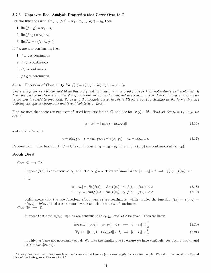
3.2.3 Unproven Real Analysis Properties that Carry Over to C

For two functions with limz→z0 f(z) = w0, limz→z0 g(z) = s0, then

1. lim(f ± g) = w0 ± s0

2. lim(f · g) = w0 · s0

3. lim f/g = w0/s0, s0 6= 0

If f, g are also continuous, then

1. f ± g is continuous

2. f · g is continuous

3. f/g is continuous

4. f ◦ g is continuous

3.2.4 Theorem of Continuity for f(z) = u(x, y) + ıv(x, y), z = x+ ıy

These proofs are new to me, and likely this proof and formalism is a bit clunky and perhaps not entirely well explained. IfI get the chance to clean it up after doing some homework on it I will, but likely look to later theorem proofs and examplesto see how it should be organized. Same with the example above, hopefully I’ll get around to cleaning up the formatting anddefining example environments and it will look better. -Lenin

First we note that there are two metrics9 used here, one for z ∈ C, and one for (x, y) ∈ R2. However, for z0 = x0 + ıy0, wedefine

|z − z0| = ||(x, y)− (x0, y0)|| (3.16)

and while we’re at it

u = u(x, y), v = v(x, y), u0 = u(x0, y0), v0 = v(x0, y0). (3.17)

Proposition: The function f : C→ C is continuous at z0 = x0 + ıy0 iff u(x, y), v(x, y) are continuous at (x0, y0).

Proof: Direct

Case: C =⇒ R2

Suppose f(z) is continuous at z0, and let ε be given. Then we know ∃δ s.t. |z − z0| < δ =⇒ |f(z)− f(z0)| < ε.

Then

|u− u0| = |Re(f(z))−Re(f(z0))| ≤ |f(z)− f(z0)| < ε (3.18)

|v − v0| = |Im(f(z))− Im(f(z0))| ≤ |f(z)− f(z0)| < ε (3.19)

which shows that the two functions u(x, y), v(x, y) are continuous, which implies the function f(z) = f(x, y) =u(x, y) + ıv(x, y) is also continuous by the addition property of continuity.

Case: R2 =⇒ C

Suppose that both u(x, y), v(x, y) are continuous at x0, y0, and let ε be given. Then we know

∃δ1 s.t. ||(x, y)− (x0, y0)|| < δ1 =⇒ |u− u0| <ε

2(3.20)

∃δ2 s.t. ||(x, y)− (x0, y0)|| < δ1 =⇒ |v − v0| <ε

2(3.21)

in which δk’s are not necessarily equal. We take the smaller one to ensure we have continuity for both u and v, andset δ = min{δ1, δ2}.

9A very deep word with deep associated mathematics, but here we just mean length, distance from origin. We call it the modulus in C, andthink of the Pythagorean Theorem for R2.

11

Now

|z − z0| < δ (3.22)

|f(z)− f(z0)| = |(u− u0)− ı(v − v0)| (3.23)

≤ |u− u0|+ |v − v0| (3.24)

<ε

2+ε

2= ε (3.25)

�

3.3 Complex Differentiation

This is a strange beast, similar but different in ways from differentiation on R2 due to the complex term. In particular, seethe Cauchy-Riemann equations below and compare to partial derivatives in R2. We still require the derivative at a point tobe the same no matter the path taken, but some interestingly fun things can happen with this (ex. f(z) = z, f(z) = z/|z|).

3.3.1 Definition and Unproven Properties from Real Analysis We Assume

To say that a derivative of f : C→ C at some z0 ∈ C exists is to say

∃ω ∈ C s.t. limz→z0

f(z)− f(z0)

z − z0= lim

∆z→0

f(z0 + ∆z)− f(z0)

∆z= ω (3.26)

and we write

f ′(z0) = ω. (3.27)

Properties: f, g continuous functions with continuous derivatives on U ⊆ C, where U is open.

1. Addition: (f ± g)′ = f ′ ± g′

2. Product: (f · g)′ = f ′ · g + f · g′

3. Quotient:(fg

)′=, I use the inverse of g and the product rule because I hate this identity, which will probably fail me

one day...

4. Chain: (f ◦ g)(z) = f ′(g(z))g′(z)

To illustrate the derivative we show a function that does not have a derivative anywhere.

Example:

Let f : C→ C, f(z) = z. Then we want to see if

lim∆z→0

f(z0 + ∆z)− f(z0)

∆z(3.28)

exists.

The limit does not exist, and to show this we approach z0 by moving parallel to the real axis (∆z = ∆x), then parallelto the imaginary axis (∆z = ∆y). Parallel to the real axis looks like

lim∆z→0

f(z0 + ∆z)− f(z0)

∆z= lim

∆x→0

x0 + ∆x+ ıy0 − x0 + lıy0

∆x(3.29)

= lim∆x→0

∆x

∆x= 1. (3.30)

Parallel to the imaginary axis looks like

lim∆z→0

f(z0 + ∆z)− f(z0)

∆z= lim

∆y→0

x0 + ıy0 + ı∆y − x0 + ıy0

ı∆y(3.31)

= lim∆y→0

ı∆y

ı∆y= lim

∆y→0

−ı∆yı∆y

= −1. (3.32)

Since these limits are not equal, the function does not have a derivative.

12

3.3.2 Cauchy-Riemann Equations, Necessary Conditions for Differentiability

Suppose f is differentiable at z0, what does this imply about u(x, y) and v(x, y)? We consider the definition of the derivativealong a path parallel to the real axis, and one parallel to the imaginary axis.

Parallel to the Real Axis:

lim∆z→0

f(z0 + ∆z)− f(z0)

∆z= lim

∆x→0

u(x0 + ∆x, y0) + ıv(x0 + ∆x, y0)− (u(x0, y0) + ıv(x0, y0))

∆x(3.33)

= lim∆x→0

u(x0 + ∆x, y0)− u(x0, y0)

∆x+ ı

v(x0 + ∆x, y0)− v(x0, y0)

∆x(3.34)

=∂

∂x(u(x, y))

∣∣∣∣(x0,y0)

+ ı∂

∂y(v(x, y))

∣∣∣∣(x0,y0)

. (3.35)

Now, parallel to the Imaginary Axis:

lim∆z→0

f(z0 + ∆z)− f(z0)

∆z= lim

∆y→0

u(x0, y0 + ∆y) + ıv(x0, y0 + ∆y)− (u(x0, y0) + ıv(x0, y0))

ı∆y(3.36)

= lim∆y→0

u(x0, y0 + ∆y)− u(x0, y0)

ı∆y+ ı

v(x0, y0 + ∆y)− v(x0, y0)

ı∆y(3.37)

=∂

∂y(v(x, y))

∣∣∣∣(x0,y0)

− ı ∂

∂y(u(x, y))

∣∣∣∣(x0,y0)

. (3.38)

Because we know that these limits must be equal, since f(z) is differentiable, then we can equate the real and imaginaryparts to get the Cauchy-Riemann Equations10

∂

∂x(u(x, y)) =

∂

∂y(v(x, y)) (3.39)

∂

∂x(v(x, y)) = − ∂

∂y(u(x, y)) (3.40)

The Cauchy-Riemann Equations are a necessary condition for differentiability, so a function that fails to satisfy the C-R Eqs.is not differentiable. To see that they are not sufficient, consider

f(z) =

{(zz

)2, z 6= 0

0, z = 0(3.41)

the proof of which is left to the reader. The hint11 is in the footnote.

One last note about the Cauchy-Riemann Equations, is that they should also be considered in polar form, considering howuseful complex exponentials are in complex analysis. As yet, this is left as an exercise for the reader.

3.3.3 Theorem of Sufficient Conditions for Differentiablity

The small addition to the Cauchy-Riemann Equations is that the derivatives of u(x, y), v(x, y) must also be continuous12.The following proposition is the theorem, but I don’t have time to work out the proof and type it up right now, so hopefullyI’ll make it back to it. - Lenin

Proposition: If u(x, y) and v(x, y) are C1 on some ε-disk w/ center at x0, y0 and they satisfy the Cauchy-Riemann Equa-tions at (x0, y0), ∃ω ∈ C s.t. f ′(z0) = ω.

3.3.4 Definitions for Functions on C

A function f on C is considered analytic on an open set U ⊆ C if f is differentiable on U .

A function that is analytic on U = C then is called an entire.

To quote Mitchell, functions that are entire are: “As nice as it gets.” “Boring.” “We want some singularities.”

10These can be solved analytically via the separation of variables with the solution left as a exercise for the reader.11Get |z|2 in the denominator, split into real and imaginary parts, take partials and equate.12The symbol, used in the proposition, for this continuity is C1, which means that the function and the first derivative are continuous, which

kind of implies the existence of the derivative. There may be a better and more rigorous way to word that (I’d bet 100 to one that there is), butit works for now.

13

3.3.5 Cauchy-Riemann in Polar Form

Hopefully when we get some free time we’ll add the derivations, but for now to use the Cauchy-Riemann Equations in polarform

r∂

∂r(u) =

∂

∂θ(v) (3.42)

∂

∂θ(u) = −r ∂

∂θ(u) (3.43)

14

4 Properties of Some Complex Functions

In this section we look at a few complex functions, some of the trouble they might cause and how to fix it.

4.1 Constant Functions, That Which Implies Them

We begin by considering what a constant function is in the Complex World, and it is very different from the Real World, butits is a useful preliminary to deal with first.

Proposition: Let f : D ⊆ C→ C. If f ′(z) = 0 ∀z ∈ D, then f is constant.

Proof: Direct

We begin by noting the functions u(x, y), v(x, y) : D ⊆ R2 → R2 for f(z) = u(x, y) + ıv(x, y), and since we have adefinition for f ′(z) = 0 = ux + ıux, it must exist, satisfy the Cauchy-Riemann Equations

ux = vy, uy = −vx (4.1)

and f ′(z) = 0 =⇒ ux = 0.

Consider a path connecting two elements in the domain of f , z1, z2 ∈ D. Now, since D is open, we can follow close to thepath by moving only parallel to the real axis or imaginary axis at a time. We will consider two legs of this journey, oneparallel to each axis and shown in Fig. 4.1.

Figure 4.1: Consider an intermediate point arbitrarily close to z1, z′.

For the first leg of our journey we move from (d, c) to (a, c), in which we have f(z) = u(x, c)+ ıv(x, c), x ∈ [d, a]. However,we know that ux = 0, which implies that f(d, c) = f(a, c) since there was no change in f by x.

The same argument holds for the second leg of the journey, (a, c) → (a, b) at z′. This process is repeated until we reachz2, and thus f(z1) = f(z2).

�

4.1.1 Corollaries and More Constant Functions

By the Cauchy-Riemann Equations, the following function definitions imply constant functions over C

1. If f is analytic and Real Value, v(x, y) ≡ 0, thus vx, vy = 0.

2. If u is constant, then all partial derivatives are always zero; same true for v.

3. If f is analytic and |f(z)| = const then13 f is constant.

4.2 The Complex Logarithm

Now we get to some real content and interesting features of the Complex World.

13This is more involved and should be proven, I’m thinking use polar forms.

15

4.2.1 The “Naive” Complex Logarithm

We14 call this the “Naive” Complex Logarithm because as we will see we will want to get rid of a multi-value output.

We begin by just considering what we want from the complex logarithm. For

z = eω (4.2)

we want

log(z) = ω. (4.3)

Consider z in polar form

z = reı(θ+2πk) = eω = eu+ıv = eueıv (4.4)

and we see that

r = eu, v = θ + 2πk (4.5)

which implies15 that

u = ln(r). (4.6)

From this we can define the natural logarithm as

log(z) = ln(r) + ı(θ + 2πk), k ∈ R (4.7)

= ln(r) + ıarg(z) (4.8)

where arg(z) indicates the angle argument of the complex number z. Since we are defining a function, we must also makesure we define its domain. The imaginary part of the logarithm is defined for all angles, however the modulus is not definedat r = 0. Additionally under this definition the complex logarithm is a function that is infinite-valued. We get z and infinite2π steps up the imaginary axis.

So, we define the logarithm as

Definition: Complex LogarithmThe Complex Logarithm is the function f : C − {0} → C, f(z) = ln(r) + ıarg(z), where r is the modulus of z andarg(z) is the angle of z, mod 2π.

4.2.2 Principle Logarithm

In order to avoid the infinite values of the complex logarithm, we define

Log(z) = ln(r) + ıArg(z) (4.9)

where Arg(z) is the Principle Angle of z, θ ∈ (−π, π].

However, the Principle Logarithm loses16 the multiplication of the real logarithm: Log(z1 · z2) 6= Log(z1) + Log(z2).

Additionally, because of the image restriction to the Principle Angle of z, the Principle Logarithm runs into differentiabilityproblems near the negative real axis. Consider moving on the unit circle from the point (1, 0) with two points, z1, z2. Thepoint z1 traces the upper semicircle, and z2 traces the lower semi-circle. As these points meet on the far end of the circle at(−1, 0) we can define z1, z2 ∈ Dδ((−1, 0)), but this does not imply f(z1), f(z2) ∈ Dε(f((−1, 0))). In fact, Log(z1) approaches(1, π) and Log(z2) approaches (1,−π). This indicates there is a series discontinuity on A = (−∞, 0]× [0].

To deal with this discontinuity we remove the set A from the domain of Log(z). Now we cannot create the same Dδ((−1, 0)),and in fact cannot create a loop that contains the origin or any negative purely real numbers. As such, we can now definethe Principle Complex Logarithm.

Definition: Principle Complex LogarithmThe Principle Complex Logarithm is the function f : C \ (−∞, 0]× {0} → (−∞,∞)× (−π, π), f(z) = ln(r) + ıArg(z),where r is the modulus of z and Arg(z) is the Principle Angle of z, θ ∈ (−π, π).

14This convention was made up while typing and we don’t yet have a different one for the distinction.15We are going to reserve the notation ln(x) to only indicate logarithms of base e when x ∈ R, as is the case for the modulus of z.16To see this use z1 = ı, z2 = ı− 1 and note that the angle summation of the right side is no longer in the image of Log(z).

16

4.3 Powers of Complex Numbers, Looking at Real Exponents

In real analysis we will do much more of this bit, but we’ll gloss over a bit to get to the fun stuff with our dear friend ı.

Let x, y,∈ R. In an expression like xm/n = y with m,n ∈ Z, we think xm = yn =⇒ x · x · · ·x = y · y · · · y, that is we have

an intuition as to what integer powers and their reciprocals mean. We have investigated this briefly with nth roots using DeMoivre’s Theorem and playing with Euler’s Form for Complex Numbers. Remember that when xq, q ∈ Q, we get a periodicanswer, namely n roots where n is the denominator of q.

But what about xa, a 6∈ Q?

In Real Analysis, we use Cauchy Sequences to say limn→∞ rn = a, rn ∈ Q, and this gives us a little bit (if of infinite com-plexity) of intuition as to what xa means. However, since we are in Complex Analysis, what about xα, α ∈ C?

Ok, the above got a little away us in tangents, and will be fixed later–hopefully. We will now consider the powers of complexnumbers of the form zα, z ∈ Z, α not yet defined. We’ll get to it. First, observe

z = elog z (4.10)

so we can write

zα = eα log z = eα(ln z+ıarg(z)+ı2πk), k ∈ Z (4.11)

= eα ln zeıarg(Z)αeı2παk. (4.12)

Now, if α ∈ Q, the last product above will be periodic with a period in k of the denominator of α. However, if α ∈ R \ Q,we lose this periodicity. Raise 1 to the power of π and see17 what happens.

A final note on powers, since they actually behave pretty nicely, if strangely, is that the complex power is likewise nice thanksto be able to split apart z = a+ bı. The quantity ıı is an interesting plot along the real axis, try it out too!

4.4 Trigonometric and Hyperbolic Functions

We begin by defining the trigonometric functions in terms of the hyperbolic

sin[x] =eıx − e−ıx

2ı= −ı sinh[ıx] (4.13)

cos[x] =eıx + e−ıx

2= cosh[ıx], x ∈ R (4.14)

which can be verified with Euler’s Identity. We do this so we can replace the real argument x with a complex argument z,and we understand what to do with ez.

Next we consider that if the argument of one of the hyperbolic functions is complex, the hyperbolic function is then periodicwith period 2πk, k ∈ Z, which is in the imaginary direction. From this we have that the trigonometric functions are periodicalong the real axis, while the hyperbolic functions are periodic along the imaginary axis.

From the definition of the trigonometric functions above, a complex argument gives

sin[z] = sin[x] cosh[y] + ı cos[x] sinh[y] (4.15)

cos[z] = cos[x] sin[y]− ı sin[x] sinh[y] (4.16)

z ∈ R, x, y ∈ R, z = x+ ıy. (4.17)

Now we want to consider the zeroes of the trigonometric and hyperbolic functions. Note their periodicity, then the trigfunctions have zeroes along the real axis, and the hyperbolic along the imaginary axis.

The trigonometric functions are no longer bounded, which can be seen by considering the magnitude squared of the a trigono-metric function with a complex argument.

When solving a function like sin[z] = 2, it is sometimes helpful to think in terms of the trig-hyper products defined above.

17Didn’t we think that 1 to the power of anything was just 1? What fun is this complexity!

17

5 Things to Do When Free Time Materialized from the Æther

1. FINISH TYPING NOTES2. Show Cauchy-Riemann in Polar Form from Rectangular

3. Implement Che’s edits and suggestions

4. Theorem of Sufficient Conditions for Differentiability

5. Prove |f(z)| = const =⇒ f(z) = const

18

6 Theorems for Final Review

6.1 Trilogy Theorem

Proposition: Suppose that a function f(z) is continuous on a domain D. If any of the following statements are true, thenso are the others. If any of the statements are false, then so are the others.

1. The function f(z) has an antiderivative F (z) throughout D.

2. The integral of f(z0 along contours lying entirely in D and

19

7 HW Problems from Complex Variables and Applications by Brown andChurchill, 9th ed.

7.1 HW One

1. Chapter 1, Section 2: 1, 2, 4

2. Chapter 1, Section 3: 1

3. Chapter 1, Section 5: 5, 6, 9

4. Chapter 1, Section 6: 1, 9, 11, 13

5. Chapter 1, Section 9: 1, 2, 5, 9, 10

6. Chapter 1, Section 11: 2, 3, 6, 7

7. Chapter 2, Section 14: 2, 8

8. Chapter 2, Section 18: 1, 5, 7

7.2 HW Two

1. Chapter 2, Section 20: 1, 8, 9

2. Chapter 2, Section 24: 1, 3, 4, 6

3. Chapter 2, Section 26: 2, 7

4. Chapter 3, Section 30: 1, 3, 6, 7, 8

7.3 HW Three

1. Chapter 3, Section 33: 2, 3, 5

2. Chapter 3, Section 36: 1, 2, 3

3. Chapter 3, Section 38: 1, 7, 8, 9, 11

4. Chapter 3, Section 39: 4, 5, 6, 8

5. Chapter 3, Section 40: 2a

6. Chapter 4, Section 42: 2, 3, 4

7. Chapter 4, Section 43: 5, 6

7.4 HW Four

1. Chapter 4, Section 46: 1, 2, 5, 13

2. Chapter 4, Section 47: 1, 3, 4, 5

3. Chapter 4, Section 49: 1, 2, 3

4. Chapter 4, Section 53: 1, 2, 3

5. Chapter 4, Section 57: 1(a, b, c), 2a, 3, 7

20