HAL Id: halshs-03157270https://halshs.archives-ouvertes.fr/halshs-03157270

Preprint submitted on 3 Mar 2021

HAL is a multi-disciplinary open accessarchive for the deposit and dissemination of sci-entific research documents, whether they are pub-lished or not. The documents may come fromteaching and research institutions in France orabroad, or from public or private research centers.

L’archive ouverte pluridisciplinaire HAL, estdestinée au dépôt et à la diffusion de documentsscientifiques de niveau recherche, publiés ou non,émanant des établissements d’enseignement et derecherche français ou étrangers, des laboratoirespublics ou privés.

Maternal depression and child human capital: A geneticinstrumental-variable approach

Giorgia Menta, Anthony Lepinteur, Andrew Clark, Simone Ghislandi,Conchita d’Ambrosio

To cite this version:Giorgia Menta, Anthony Lepinteur, Andrew Clark, Simone Ghislandi, Conchita d’Ambrosio. Mater-nal depression and child human capital: A genetic instrumental-variable approach. 2021. �halshs-03157270�

WORKING PAPER N° 2021 – 10

Maternal depression and child human capital: A genetic instrumental-variable approach

Giorgia Menta Anthony Lepinteur

Andrew E. Clark Simone Ghislandi

Conchita D’Ambrosio

JEL Codes: I14, J24 Keywords: Mendelian Randomisation, Maternal Depression, Human Capital, Instrumental Variables, ALSPAC.

Maternal depression and child human capital:

A genetic instrumental-variable approach*

GIORGIA MENTA University of Luxembourg

giorgia.menta@uni.lu

ANTHONY LEPINTEUR University of Luxembourg

anthony.lepinteur@uni.lu

ANDREW E. CLARK Paris School of Economics - CNRS

Andrew.Clark@ens.fr

SIMONE GHISLANDI Bocconi University

simone.ghislandi@unibocconi.it

CONCHITA D’AMBROSIO University of Luxembourg

conchita.dambrosio@uni.lu

This version: February 2021

Abstract

We here address the causal relationship between maternal depression and child human capital

using UK cohort data. We exploit the conditionally-exogenous variation in mothers’ genomes

in an instrumental-variable approach, and describe the conditions under which mother’s genetic

variants can be used as valid instruments. An additional episode of maternal depression

between the child’s birth up to age nine reduces both their cognitive and non-cognitive skills

by 20 to 45% of a SD throughout adolescence. Our results are robust to a battery of sensitivity

tests addressing, among others, concerns about pleiotropy and the maternal transmission of

genes to her child.

Keywords: Mendelian Randomisation, Maternal Depression, Human Capital, Instrumental

Variables, ALSPAC.

JEL Classification Codes: I14, J24.

* We would like to thank Aysu Okbay for her comments and assistance with the GWAS summary data, and Niels Rietveld

for sharing his codes with us. We are very grateful to Sonia Bhalotra, Pietro Biroli, Dalton Conley, Maria Cotofan, Jan-

Emmanuel De Neve, Emilia Del Bono, Martin Fernandez-Sanchez, Sarah Flèche, Richard Layard, Andrew Oswald, Steve

Pischke, Alois Stutzer, Felix Tropf, and participants at the First Social Science Genetics Paris meeting, the IGSS conference,

the EuHEA, the University of Luxembourg, and the University of Oxford Wellbeing seminars for useful comments. We are

extremely grateful to all the families who took part in this study, the midwives for their help in recruiting them, and the whole

ALSPAC team, which includes interviewers, computer and laboratory technicians, clerical workers, research scientists,

volunteers, managers, receptionists and nurses. The UK Medical Research Council and the Wellcome Trust (Grant ref:

217065/Z/19/Z) and the University of Bristol provide core support for ALSPAC. A comprehensive list of Grants funding is

available on the ALSPAC website (http://www.bristol.ac.uk/alspac/external/documents/grant-acknowledgements.pdf).

Genotype data were generated by Sample Logistics and Genotyping Facilities at Wellcome Sanger Institute and LabCorp

(Laboratory Corporation of America) using support from 23andMe. This publication is the work of the authors and all authors

will serve as guarantors for the contents of this paper. Financial support from the Fonds National de la Recherche Luxembourg

(Grants C19/SC/13650569 and 10949242) is gratefully acknowledged. Andrew Clark acknowledges financial support from

the EUR grant ANR-17-EURE-0001.

1

1. Introduction

The prevalence of mental-health disorders has been rising steadily for over two decades

(Stansfeld et al., 2016), and these are now estimated to affect over 20% of the population in

the UK (www.mind.org.uk) and the US (www.nami.org/mhstats). Depression is one of the

most common of these disorders. A vast literature has documented worse outcomes for the

depressed in terms of not only health, but also employment and earnings (Zimmerman and

Katon, 2005; Fletcher, 2013; Banerjee et al., 2017; Hakulinen et al., 2019), productivity

(Bubonya et al., 2017), marital status and marital satisfaction (Gotlib et al., 1998), and

parenting style (Kiernan and Huerta, 2008). Major Depressive Disorder has been identified as

the largest worldwide contributor to years lost to disability (Prince et al., 2007).

Depression in addition, likely also spills over onto others. There is a great deal of work on

the intergenerational correlation between parental and child depression (see Gotlib et al., 2020,

for a recent summary). We here consider the consequences of maternal depression on child

human-capital in unique British birth-cohort data, beyond the intergenerational inheritance of

the genes associated with depression.

While a broad range of descriptive evidence has underlined the negative association

between maternal depression and child outcomes (see Goodman et al., 2011, and O'Hara and

McCabe, 2013, for meta-analyses and reviews of the psychological literature), there has been

little causal analysis of this intergenerational link. One exception is Dahlen (2016), who uses

non-parametric bounds to estimate ranges of the negative causal impact of maternal depression

on the test scores and socioemotional outcomes of US kindergarten children. More notably,

von Hinke et al. (2019) rely on unexpected life experiences (the illness or death of friends and

family members) to isolate the effect of perinatal maternal depression on children’s cognitive

and non-cognitive skills in a UK birth cohort (ALSPAC; the same dataset that we use here).

They find that mother’s worse mental health around birth negatively affects their children’s

non-cognitive skills, with the effects fading away as the child approaches adolescence. No

effect is found on cognitive outcomes.

A small number of contributions have focused on the beneficial causal effects of the

successful treatment of depressed mothers. Perry (2008), exploiting the arguably-exogenous

variation in US primary-care physicians’ propensity to diagnose depression, shows that treating

maternal depression improved children’s asthma outcomes. Using data from a randomised

controlled trial, Baranov et al. (2020) find that prenatally-depressed mothers in rural Pakistan

who were offered psychotherapy had better mental-health outcomes, and invested more time

2

and money in their children (although there is only limited evidence that this investment

improved child-development outcomes).

The causal link between parental mental health and child outcomes is of primary policy

importance, but is in general not particularly easy to establish. The interplay between maternal

mental health and child human-capital development is complex and subject to potential

endogeneity concerns. For instance, poor child school performance or behavioural problems

might themselves produce maternal depression; alternatively, environmental variables (shared

by parents and children who live in the same household), such as local public goods or

criminality, could feed through to both parental mental health and child outcomes. In both cases

it is difficult to establish causality.

We here address endogeneity via recent advances in Epidemiology and Molecular Genetics.

In particular, we adopt a genetic instrumental-variable approach (similar to DiPrete et al.,

2018), and instrument maternal depression using a synthetic measure (the polygenic score)

based on the mother’s genetic variants that are robustly associated with the trait of depression.

Our empirical analysis is based on genetic and socio-economic information on mother-child

pairs from the Avon Longitudinal Study of Parents and Children (ALSPAC), a UK-based

cohort study that recruited about 14,000 pregnant mothers in the early 1990s. The key

explanatory variable is reported maternal depression: this is a summary measure from the

answers mothers give to questions about recent depression in seven different data waves from

childbirth up to child age nine. We instrument this cumulative depression score by the

polygenic score (PGS) for maternal depression, using Genome-Wide Association Studies

(GWAS) summary statistics from the depression meta-analysis in Turley et al. (2018). Our

methodological approach is similar to that in von Hinke et al. (2016), who illustrate the

assumptions under which an individual’s genetic variants can be used as instrumental variables

for that individual’s traits (in their empirical application, child fat mass). Our question differs

from theirs, as the trait we instrument (depression) and the outcome (human capital) refer to

different individuals (respectively, the mother and her child). In this intergenerational analysis,

additional concerns need to be addressed, such as those deriving from genetic inheritance that

we will discuss below.

Following the human-capital development and skill-formation literature (see, for example,

Cunha and Heckman, 2008), we consider child cognitive and non-cognitive skills as human

capital components. The cognitive element is given by the measurement of child skills and

knowledge at different stages of compulsory education in the UK. We in particular analyse the

child’s average Key Stage test-scores at ages 11 and 14, and their total GCSE score at age 16

3

(at the end of compulsory education); all three of these test scores come from administrative

data. Non-cognitive skills come from the child’s score from the questions in the Strengths and

Difficulties Questionnaire (as reported by their principal carer) at child ages 11, 13 and 16.

The genetic instrument allows us to isolate an exogenous change in maternal depression up

to child age nine and establish its causal impact on the child’s later human capital. We find that

one additional episode of maternal depression (out of the seven recorded) has a persistent

negative impact on both cognitive and non-cognitive skills, with an effect size of around 20%

of a standard deviation for the former and 40% for the latter.

Our identification strategy relies on a number of assumptions: while the relevance of the

mother’s PGS in predicting her depression can be formally tested, the genetic nature of this

instrument calls for a more thorough investigation of the exclusion restriction. We illustrate

the potential pathways that may compromise identification here, and discuss some ways in

which these concerns can be addressed. Pleiotropy (when one genetic variant can explain a

number of different traits) is arguably the main issue with genetic instrumentation in general.

The intergenerational nature of our research introduces a second potential problem, that of

genetic inheritance: as the child inherits about 50% of each parent’s genetic variants, the direct

effect of the child’s inherited genetic variants may confound the relationship between mother’s

instrumented depression and child human capital. Child outcomes will be affected by the

child’s own depression, and this is partly due to the genetic propensity for depression that was

inherited from the mother. But this is not what we understand by asking if depressed mothers

affect their children’s outcomes: we here rather wish to establish the effect of maternal

depression net of genetic inheritance.

We tackle some of the pleiotropic concerns by controlling for a set of maternal and child

traits that might be affected by the genetic variants used in the construction of the PGS, and

that are in turn likely to affect human-capital development (e.g. educational attainment and

fertility decisions). Following Lawlor et al. (2017) and DiPrete et al. (2018), we control for

genetic inheritance by holding constant the child’s own PGS for depression, as well as their

PGSs for cognitive and non-cognitive skills. Our results are robust to these and other sensitivity

tests.

The remainder of this paper is organised as follows. Section 2 describes the birth-cohort

data that we use. Section 3 then provides an overview of the conditions under which genetic

variants can be used as instrumental variables in observational data, and considers the specific

issues when the treatment and the outcome refer to different individuals who are genetically-

related. The main results, of a sizeable causal effect of maternal depression in childhood on

4

adolescent children’s cognitive and non-cognitive skills, and a variety of robustness checks,

appear in Section 4. Last, Section 5 concludes.

2. Data: The Avon Longitudinal Study of Parents and Children

We will use mother’s genetic information as an instrument to establish the causal effect of

her depression on her children’s cognitive and non-cognitive outcomes. The data requirements

to carry out this analysis are stringent. We need information on mother’s reported depression

during her child’s young years, the adolescent outcomes of her child, and both the the mother’s

and the child’s genotype. Few datasets contain all of this information. One that does is the

Avon Longitudinal Study of Parents and Children (ALSPAC) survey, also known as ‘The

Children of the 90s’.

ALSPAC is an English birth-cohort study designed to investigate the influence of

environmental, genetic, and socio-economic variables on health and development over the life

course. Over 14,000 pregnant women who were due to give birth between April 1991 and

December 1992 in the county of Avon (Bristol and its surrounding areas) were recruited. These

women and their families have been followed ever since, even if they move out of the original

recruitment area (see www.bristol.ac.uk/alspac/). The pregnancy outcomes of the participants

resulted in a total of 14,062 live births, with 13,988 children surviving their first year. The

sample is broadly representative of the early 1990s UK population of mothers with children

under age one, although higher socio-economic status groups as well as Whites are over-

represented (see Fraser et al., 2013, and Boyd et al., 2013, for a full description of the cohort

profile). The study includes detailed information about the family environment, as well as

indicators of child development, wellbeing and skills over time, and rich information on the

parents’ characteristics and background.1 Biological samples from the children and their

parents were collected at different points in time, allowing for DNA genotyping. We here use

imputed genotype data from around 9,000 children and their mothers (Taylor et al., 2018,

provide technical details on the genotyping technology, imputation, and quality control in

ALSPAC).

When the child was aged 8 months and 2, 3, 4, 5, 6 and 9 years, their mothers were asked

whether they had experienced depression since the last interview in which they were asked

about their health (or since the birth of the child the first time this question was asked).

1 The study website contains details of all the data that is available through a fully searchable data dictionary and

variable search tool: http://www.bristol.ac.uk/alspac/researchers/our-data/.

5

Although the wording of the question changed slightly across waves, the potential responses

were the same: “Yes and consulted a doctor”, “Yes but did not consult a doctor” and “No”. We

consider a mother to have had an episode of depression between two periods if she replied

“Yes and consulted a doctor” or “Yes but did not consult a doctor”. We combine these seven

reported depression scores to produce an index of reported maternal depression from the child’s

birth to the child’s ninth birthday, with index values running from zero to seven.

Our child non-cognitive skill measures come from the Strengths and Difficulties

Questionnaire (SDQ) (as used in Flèche, 2017; Briole et al., 2020; and Clark et al., 2021). The

SDQ is a 25-question behavioural-screening tool for children, including questions on whether

the child is considerate of others, and her concentration span, worries and fears, degree of

obedience, and social isolation (Goodman, 1997). The full list of the SDQ items appears in

Appendix Table A1. The main carer (this is the mother in the vast majority of cases) was asked

to rate the child’s SDQ seven times between child ages 4 and 16. We will relate maternal

depression during the child’s first 9 years to the child’s subsequent SDQ scores at ages 11, 13

and 16.

The 25 SDQ items are split up into five sub-scales covering emotional problems, peer

problems, conduct problems, hyperactivity/inattention and pro-social behaviour. Consistent

with Goodman et al. (2010) and the SDQ scores produced by ALSPAC, our main analysis will

use the total SDQ score, which is the sum of the first four sub-scales. We code total SDQ so

that higher values represent better outcomes (i.e. strengths rather than difficulties). In the

robustness checks (Section 4.4.2), we will consider additional non-cognitive skill measures to

test for convergent validity (teacher-reported SDQ scores, and an alternative measure of non-

cognitive skills from the Short Moods and Feelings Questionnaire, SMFQ, reported by the

main carer).

Child cognitive development is measured by their national exam results in linked

administrative data from the UK National Pupil Database. We use the average Key Stage fine-

grading test-scores at ages 11 and 14 and the total GCSE score in all of the exams that the child

took at the end of compulsory education at age 16.2

The next section first sets out the principle of using genotype data as an instrument, and

then describes the way in which we will apply this method using ALSPAC data.

2 At the end of Key Stages 2 (age 11) and 3 (age 14), children’s progress in Mathematics, Science and English is

assessed using National Curriculum tests. While these tests do not produce exit certificates, the national exams

taken at the end of Key Stage 4 (age 16), the General Certificate of Secondary Education (GCSE), do produce

qualification certificates. Students in the UK typically take at least 5 GCSEs (one per subject), with Mathematics,

Science and English being compulsory.

6

3. A Genetic Instrumental-Variables Approach

3.1. Mendelian Randomisation

Establishing causality in non-experimental data is very often challenging, and particularly

so for variables that are unlikely to be targeted by policies or be subject to quasi-experimental

variation. One recent approach in Social Sciences and Epidemiology is Mendelian

Randomisation (MR). This term refers to Mendel’s Laws of Segregation and Independent

Assortment, which are involved in the formation of reproductive cells (i.e. gametes) through

meiosis and which ensure genetic variability across individuals. Traits that are regulated by

one gene are defined by a sequence of two alleles (one inherited from each parent); the Law of

Segregation states that each individual has a 50% chance of inheriting one of the two maternal

(paternal) alleles for a given gene. The Law of Independent Assortment, on the other hand,

ensures that alleles for different traits are passed on independently of each other.3 As a result,

conditional on the parental genotypes, the child’s genotype can be seen as the outcome of a

lottery.4

MR in practice refers to a variety of different approaches, the common denominator being

the use of genetic variants as instrumental variables for a given endogenous trait (see

Koellinger and De Vlaming, 2019, and Hemani et al., 2018, for reviews of some recent

developments). While some traits can be linked to a clear small set of genetic variants through

well-characterised biological pathways (this is the case for severe health problems, such as

Huntington’s disease), most traits that interest economists and other social scientists (e.g.

socio-economic status, education, and subjective well-being) are highly polygenic and, as such,

involve a greater degree of genetic complexity. The burgeoning literature on large-scale

GWAS, which aims to estimate the relationship between a given trait and known genetic

variants (typically Single-Nucleotide Polymorphisms, or SNPs) in large samples, has brought

about significant advances in the understanding of the genetic architecture of genetically-

complex traits such as education (Lee et al., 2018; Demange et al., 2021), depression (Okbay

et al., 2016; Turley et al., 2018) and risk behaviour (Karlsson Linnér et al., 2019).

One issue with the use of genetic variants of complex traits as instrumental variables is

weak instruments, as each single SNP identified in a GWAS likely has only relatively little

3 The Law of Independent Assortment does however come with a caveat: genes that are close to each other on a

chromosome strand have a higher chance of being transmitted together. This leads to what is known as linkage

disequilibrium: in a given population, alleles for different genes have higher association rates than those that

would be expected from random matching. 4 Note that if parents were to match to each other independently of the trait that a given genotype regulates, we

would not even need to condition on parental genotypes for the genotype of the child to be a random draw from

the population genetic pool.

7

predictive power on its own. Polygenic scores have then come into widespread use as linear

combinations of all of the relevant genetic markers into one synthetic measure (Appendix B

provides more details on the PGS and its functional form), capturing a greater portion of trait

variance as compared to single SNPs (DiPrete et al., 2018; Davies et al., 2015).

We now consider the various relationships between maternal genes and her child’s

outcomes, and how these can be addressed to establish a plausible causal relationship.

3.2. Instrumental Variable Assumptions in the Context of Genetic Instruments

While others have laid down the assumptions for drawing inference from genetic

instruments within the same individual (notably von Hinke et al., 2016), we here consider

instrumentation between parent and child, as illustrated by the solid black lines in Figure 1. We

aim to measure the causal effect of a mother’s trait DM on her child’s outcome YC (i.e. the value

of the parameter β), where GMD

is a vector of independent genetic variants of the mother that

are robustly associated with this trait DM. In the ALSPAC analysis that we undertake here, DM

is maternal depression between child birth and child age nine, YC the adolescent-child’s human

capital, and GMD

the mother’s PGS for depression, based on the 88 most-relevant SNPs (p-value

threshold of 10–6) derived from the single-trait meta-analysis in Turley et al. (2018). The results

throughout the paper are robust to the use of a more-stringent threshold, identifying what are

called genome-wide significant SNPs, with a p-value threshold of 5×10–8.

Just as in a standard instrumental variables (IV) analysis, the validity of the identification

strategy relies on the following assumptions:

- Relevance: the genetic variants GMD

are correlated with the trait DM (α ≠ 0).

- Independence: the GMD

are not correlated with any confounders (𝑈) of the association

between the mother’s trait and the child outcome (η = 0).

- Exclusion restriction: the GMD

are causally related to the outcome YC only through the

trait DM (so that β is not confounded by any of the dashed grey lines in Figure 1).

The relevance assumption, while being the easiest to prove in most IV contexts, is

particularly straightforward in the case of genetic instrumental variables. The task of

identifying which genetic variants are robustly associated with a given trait is typically left to

summary data from published GWAS (see Appendix B for further details). As noted above,

single genetic variants per se might not be sufficiently strong predictors of a trait, especially

when the latter is genetically-complex. In these cases, it is more appropriate to use synthetic

measures such as the PGS to avoid weak-instrument problems.

8

The independence assumption is typically assumed to hold in the context of MR due to the

randomness of genetic variants, with very few exceptions suggesting otherwise (e.g. Koellinger

and De Vlaming, 2019). It is worth underlining, however, that the mother’s genotype can be

considered as truly random only when conditioning on the maternal grandparents’ genotype.

In practice, for data-availability reasons, it is seldom possible to partial out the genes of the

mother’s parents when analysing GMD

. Some common established good practices in MR

analyses are controlling for population stratification5 and documenting the absence of

systematic correlations between the instrument and observable confounders (Smith et al., 2007;

Boef et al., 2015).

In the context of multivariate regressions, controlling for a selected set of grandparental

traits, as well as environmental characteristics, should also attenuate the concerns regarding the

independence assumption. Consider, as an illustration of U in Figure 1, the potential influence

of grandparental depression. Depressed grandparents are first more likely to have genetic

variants associated with depression: via genetic inheritance, their daughters will then also likely

display a higher PGS for depression (in Figure 1 this would translate into 𝜂 ≠ 0). In addition,

grandparental depression may increase the chances of their daughter’s depression through non-

genetic pathways, e.g. by increasing familial stress and anxiety (this is represented by the line

from U to DM in Figure 1). Last, grandparental depression can affect child outcomes directly,

as depicted in the line from U to YC: this could reflect, for example, the crowding-out effect of

the time that mothers with depressed parents can dedicate to their children. As they may

simultaneously affect all of the variables of interest (via the three unbroken grey lines in Figure

1), not controlling for grandparental genes and/or their associated traits can violate the

independence assumption.6 Introducing controls for the depression of both of the grandparents,

as well as for other grandparental traits and environmental characteristics, can attenuate the

bias in this case.

The exclusion restriction is well-known to be the most problematic assumption in all IV

setups, and this is particularly true in the context of MR (Koellinger and De Vlaming, 2019).

5 This stratification reflects drifts in allelic frequencies within the population of interest. A popular solution, which

is particularly well-suited in contexts of considerable geographical and ethnic diversity, is controlling for principal

components derived from genotyped data. These account for systematic associations between the alleles in subsets

of a given population that are produced, among other things, by within-group assortative-matching patterns. 6 While the grandparents’ non-transmitted alleles can be unobserved confounders of the DM - YC association

(through genetic nurture, as they likely affect the way in which the grandparents bring up the mother), they do not

play a role in the independence assumption of the effect of GMD on YC, as they cannot appear in the mother’s PGS

for depression (Mendel’s Law of Segregation).

9

In our mother-child framework, phenomena such as horizontal pleiotropy and genetic

inheritance can link GMD

and YC through pathways other than DM.

Under horizontal pleiotropy, an individual’s genetic variant directly affects two or more of

her traits through separate biological pathways (e.g. the genetic variants causing maternal

depression might also affect other maternal traits, such as educational attainment). This will

pose identification problems if these additional traits affected by GMD

(the XM in Figure 1) are

correlated with the outcome of interest (γ1 ≠ 0).

One simple way to account for the confounding effects of the XM in Figure 1 is to control

for them. While this may sound rather trivial, most MR applications are actually bivariate

associations (accompanied, in most cases, by statistical tools to account for pleiotropy),

typically due to data limitations. We do of course need to be careful when controlling for

maternal traits: while some might indeed capture part of the observable pleiotropic effects, they

can also partly mediate the relationship between DM and YC and, as such, be ‘bad controls’

(Angrist and Pischke, 2008). In relation to Figure 1, holding ‘bad controls’ constant would lead

to the attenuation of the estimated value of β.

Genetic inheritance also poses a problem for identification. Each child inherits 50% of each

parent’s genetic variants. This produces the path from GMD

to GCD

, the child’s genetic variants

that are associated with child trait D, in Figure 1. There are then two pathways from GCD

to the

child’s outcome. The first is the direct biological pathway from GCD

to YC (δ1 ≠ 0); the second

is due to vertical pleiotropy (γ2 ≠ 0), i.e. the effect of GC

D on YC that is mediated by one or more

child traits (XC).

The issues around genetic inheritance might not only concern the transmission of the

genetic variants for depression. The child’s genetic variants explaining YC, GCY may also partly

be inherited from the mother’s GMD

and/or result from linkage disequilibrium (LD from here

onwards; see footnote 3 for the definition) with it (δ2 ≠ 0). This is important here, as mental

health and cognitive achievement partly share the same genetic aetiology (see Rajagopal et al.,

2020). Similarly to GCD, the vector GC

Y can affect the child outcomes either directly or via

vertical pleiotropy (γ2 ≠ 0).

Were the genetic data detailed enough, we could deal with all the concerns arising from

genetic inheritance by using only the mother’s non-transmitted alleles as instruments:

mechanically, there would then be no correlation between the mother’s and the child’s

genotypes (unless there is assortative matching between the parents over trait D and/or Y).

10

Another possibility, which is what we do here, is to control for the child’s genotypes, so as to

hold constant all of the pathways between GCD

, GCY and YC. We will in addition control for the

child’s traits, XC, in case these partly result from genetic variants other than GCD

and GCY. We

are to the best of our knowledge the first to be able to control for both the child’s PGS for

depression, GCD

(Lawlor et al., 2017), and cognitive (non-cognitive) skills, GCY (DiPrete et al.,

2018),7 in the empirical analysis. Note that once we have controlled for the relevant child PGSs,

the residual part of the bivariate pathway between XM and YC in Figure 1, γ1 , reflects genetic

nurture (Kong et al., 2018), i.e. the effect of the maternal traits caused by the part of GMD

that is

not inherited by the child.

We next describe the equations that to be estimated using ALSPAC data.

3.3. Empirical Strategy

We address endogeneity by estimating the following Two-Stage Least Squares (2SLS)

regressions using a genetic instrument:

DM = α1PGSMD

+ α2XM + α3XC + α4PCM + ϵM (1)

HKCt = β1DM + β

2XM + β

3XC + β

4PCM + υCt. (2)

In Equation (1), DM is the number of self-reported episodes of maternal depression, from

the child’s birth up to age nine, taking on values from 0 to 7. In Equation (2), the outcome HKCt

is successively different measures of child C’s human capital at age t : the fine-grading average

Key Stage test-scores at ages 11 and 14, the total GCSE score at age 16, and total (carer-

reported) SDQ at child ages 11, 13 and 16. We standardise the different HKCt variables for

comparison purposes, as they are not measured on the same scale.

We address pleiotropy by controlling for a set of both mother and child traits. XM is a vector

of mother’s traits when the child is aged nine: age at the birth of the child and dummies for

being employed, having at least an A-level,8 having a partner, having a partner with at least an

7 Note that controlling for GC

Y is what DiPrete et al. (2018) refer to as Unconditional Genetic Instrumental

Variables (GIV-U), that is simply controlling for all the genetic variants associated with 𝑌𝐶 (i.e. GCY ). In particular,

they show that GIV-U regression provides a reasonable lower bound for the true effect of DM on YC under several

violations of the IV assumptions (either through moderate pleiotropy or other genetic confounds). 8 An A-level (Advanced Level) qualification is a subject-based school-leaving certificate that is typically obtained

at the end of Upper-Secondary School at around age 18.

11

A-level, having an employed partner, the number of additional children, and banded household

income (the latter two variables are measured at child age 8). It can be argued that some of

these are potentially bad controls, as they may themselves be influenced by maternal depression

(for example, mother’s labour-force status and the household’s income). We will address this

issue in the robustness checks. Last, the XC are time-invariant child traits: gender, birth year

and birth order.

In Equation (1), PGSMD

, the maternal polygenic score for depression (our measure of

mother’s genetic variants, GMD

, in Figure 1) is used as an instrument for maternal depression

DM. We calculate PGSMD

using the command-line program PLINK 1.9, with summary statistics

from the single-trait depression meta-analysis GWAS in Turley et al. (2018). 68 of the 88 SNPs

identified in the GWAS are genotyped in ALSPAC participants and were used in the PGS: see

Appendix B for the details of the calculation. We standardise PGSMD

, as polygenic scores have

no natural scale. With polygenic scores being based on genetic variants that are determined at

conception, the exogenous variation in maternal depression provided by PGSMD

is fixed prior

to the child’s birth: this rules out reverse-causality concerns (e.g. mothers’ mental health being

affected by their children’s poor cognitive and/or non-cognitive performance).

We address population stratification by excluding mothers of non-European descent:

Hansell et al. (2015) find no evidence of any remaining population stratification in ALSPAC

after this selection and other standard quality-control (QC) procedures (see Taylor et al., 2018,

for a complete overview of the QC procedures that were applied to ALSPAC data prior to its

release). While the documented lack of stratification provides evidence in favour of the

independence assumption in our context, we always control for 10 ancestry-informative

principal components PCM (as in von Hinke et al., 2016) and carry out additional tests for the

influence of grandparental characteristics and partners’ depression on the effect of maternal

depression (see Section 4.3).

Our estimation sample consists of observations with non-missing values for mothers’

genetic information, depression history, and the controls measured at child age nine.9 As there

are only 1,065 families with non-missing information on all six human-capital measures and

we cannot reject concerns about weak instruments in this balanced sample, we here use a

9 The mother’s traits that are measured at child age eight (household income and the number of children in the

household) are missing in roughly 9% of the cases in our different estimation samples. Where the respondents

have missing information, we create a variable-specific dummy to flag this missing information (the Missing

Indicator method) and replace the missing value by the sample mean. We in addition drop the 32 cases with

multiple births for the mother over the 18-month initial survey period (although our results are robust to including

these observations).

12

different estimation sample for each dependent variable to maximise statistical power. Our

final samples consist of between 2,036 and 2,993 observations per equation estimated. Due to

attrition, the size of the non-cognitive skills estimation samples falls naturally with child age

(from 2,993 to 2,076 observations). For cognitive skills, the estimation samples consist of 2,828

observations at age 16 (GCSE), 2,601 observations at age 11 (KS2) and 2,036 at age 14 (KS3).

The discrepancy between the sample sizes at age 16 and earlier child ages reflects that the

average KS2 and KS3 grades are retrospectively matched when the child takes her GCSE

exams at age 16. 10% of the 227-observation difference between the GCSE and KS2 samples

is due to either missing values in the school and academic year identifiers or in the grades,

while the remaining 90% is due to the NPD data-cleaning process. For the gap between the

GCSE and KS3 samples, 258 observations are missing for these two reasons, while the

remaining 534 are due to the KS3 grades of ALSPAC children taking their GCSE in academic

year 2008-09 no longer being collected.10 The influence of maternal depression and PGSMD

on

attrition and the different sample sizes is discussed in the next section.

The distribution of self-reported maternal depression in the different estimation samples

appears in Table 1, where depression takes on values between zero and seven. Around half of

the women in our samples reported at least one episode of depression between the birth and

ninth birthday of their child. This figure is consistent with data from a nationally-representative

survey, the British Household Panel Study (BHPS), over the same time period: around 45% of

the mothers observed for at least two consecutive years from 1991 to 2000 reported a least one

episode of depression. The distribution of the measures of children’s human capital is shown

in Appendix Figure A1, and the complete descriptive statistics are listed in Tables A2

(cognitive skills) and A3 (non-cognitive skills).

While Equation (2) partly addresses pleiotropy by controlling for both the mother’s and the

child’s traits (XM and XC), the maternal PGS may still be directly linked to child human capital

via the child’s genome (GCD

and GCY in Figure 1). We here follow Lawlor et al. (2017) and

DiPrete et al. (2018), and address these concerns by controlling for the child’s PGS for

depression and, respectively, cognitive and non-cognitive outcomes (see Section 4.2.3).

10 Technical details about the NPD cleaning process and the collection of the KS3 average grades we use here can

respectively be found at http://www.bristol.ac.uk/media-library/sites/cmpo/migrated/documents/

ks5userguide2011.pdf and https://find-npd-data.education.gov.uk/en/data_elements/11e50a8a-78d6-425c-871d-

9d9fd3330dd9.

13

4. Results

4.1. Main Results

Table 2 presents the OLS and 2SLS estimates of Equation (2) for the effect of maternal

depression on the different measures of child human capital. All of the estimated coefficients

are negative and significantly different from zero at the 10% level at least. In the 2SLS results

in columns (2), (4) and (6), one additional episode of maternal depression before child age nine

reduces child test-scores by on average 23% of a standard-deviation (SD) and total SDQ by

roughly 45% of a SD.11 Although the 2SLS estimates become a little larger as the child grows

older, none of them are significantly different from each other. This pattern does not reflect the

different sample compositions: restricting our analysis to families with valid information on

either all of the cognitive-skill measures or all of the non-cognitive skill measures yields similar

conclusions (these results are available upon request). Our specification exploits the

longitudinal dimension of the dataset by looking at the impact of the observed history of a

mother’s depression on the subsequent cognitive and non-cognitive outcomes of her children.

Our estimates may thus reflect the predictive effect of the PGS on unobserved later episodes

of maternal depression occurring between child age nine and the time the child’s outcome of

interest is observed. Maternal depression during a child’s puberty could have a greater impact

on their schoolwork and behaviour, producing larger coefficients at ages 14 and 16. In either

case, maternal depression produces worse child outcomes.

Instrument relevance is evaluated in the first-stage estimates below the 2SLS results in

Table 2. As expected, a higher PGS for depression significantly predicts more maternal-

depression episodes in all specifications (at the 0.1% level at least). We also list the Cragg-

Donald Wald F-statistics for the first-stages, which are sufficiently large to alleviate weak-

instrument concerns in most cases.12 This F-statistic is under 10 only for the effect of maternal

depression on total SDQ at age 16, which may show selective attrition. The probability of

dropping out of the total SDQ estimation sample between two periods rises with maternal

11 The reduced-form estimates for the PGS for depression range from -0.036 to -0.051 SD for cognitive skills and

from -0.071 to -0.063 SD for non-cognitive skills, with significance levels identical to those in our baseline 2SLS

estimates. While reduced-form estimates rely on weaker assumptions, they come at a cost in terms of

interpretation, as they do not identify a mediating trait in the maternal genes - child outcome relationship. Under

the assumptions described in Section 3.2, our 2SLS estimates reveal that the causal effect of the PGS for

depression of the mother on the human child capital of children is only mediated by maternal depression. 12 We cannot make strong statements about whether the effect of maternal depression differs by gender, birth-

order, maternal education and household-income band, as the smaller samples produce F-statistics that are mainly

too low for robust inference.

14

depression, but does not depend on the value of the instrument. It is thus unsurprising to see a

lower first-stage F-statistic in the last column of the bottom panel of Table 2.13

Columns (1), (3) and (5) show the OLS results. Although these are qualitatively similar to

the 2SLS estimates, they are four to ten times smaller in size. This gap may reflect that the

GWAS summary statistics from Turley et al. (2018) are based on discovery samples where the

trait is mostly measured as clinically diagnosed depression or self-diagnosed major depressive

disorder (in around 80% of cases). As such, it is normal that the 2SLS estimates be larger than

those in OLS, as the instrument captures more extreme forms of depression, that in turn play a

larger role in human-capital accumulation. When analysing a non-binary trait (like our measure

of maternal depression) genetic compliers can be seen as the whole population (see Dixon et

al., 2020). Our 2SLS estimates then capture the average treatment effect of the trait that is most

prevalent in the GWAS discovery cohorts – that is, ‘severe’ forms of depression (clinically-

diagnosed depression, or major depressive disorder). On the contrary, the OLS estimates reveal

the average effect of all forms of depression, both mild and severe.

The difference between the OLS and 2SLS estimates is larger for cognitive than non-

cognitive skills: this may reflect the relative importance of diagnosed and undiagnosed

symptoms of maternal depression in these two dimensions of human capital. While we do not

observe formal diagnoses of depression, we know whether the mother consulted a doctor due

to her depressive symptoms. When we separately consider episodes of maternal depression that

were followed up by a medical visit and those that were not, the descriptive evidence from the

OLS estimates suggests that, while both measures matter equally for non-cognitive skills, only

the former is significantly associated with child cognitive skills (results available upon

request).14

13 Note that neither maternal depression nor the instrument predict retrospective attrition for cognitive skills in the

top panel of Table 2. As information on Key Stages 2 and 3 (child ages 11 and 14, respectively) test-scores are

obtained retrospectively, attrition here is the probability of being in the age-16 sample for cognitive skills and

being absent from, respectively, the analogous age-11 and age-14 samples. The results on attrition in the cognitive

and non-cognitive samples are available upon request. 14 It might be thought then that we would be better-off restricting our analysis only to episodes of maternal

depression that are followed by a medical consultation. When doing so, we find coefficients that are on average

twice as large as the baseline 2SLS estimates from Table 2 (all significant at least at the 10% level). However, the

F-statistics for episodes of maternal depression followed by a medical visit take values that are systematically

lower than those in Table 2. Using only depressive episodes followed by a medical visit comes at a greater risk of

weak-instrument issues.

15

4.2. Addressing the Exclusion Restriction

4.2.1. Horizontal Pleiotropy

The credibility of the exclusion restriction relies on there being no relationship between the

PGS for maternal depression and the child outcomes, other than via maternal depression.

However, as set out in Section 3.2, a genetic variant may predict more than one trait: this is

horizontal pleiotropy. While we already control for a set of maternal traits in our main

specification, we here provide additional evidence against pleiotropy playing a significant role

in our analysis. Table A4 in Appendix A shows the bivariate associations between the PGS for

depression and a variety of maternal traits. Unsurprisingly, the association between the PGS

and maternal depression is positive and very significant. Just as importantly, none of the other

traits is significantly associated with this instrument. While we cannot entirely rule out an effect

of the genetic variants in the mother’s PGS on other unobserved traits involved in child human-

capital development, the lack of any correlation with the observed traits is reassuring.

We also address the risk of pleiotropy more directly, investigating the known biological

functions that are linked to the 68 SNPs used in the mother’s PGS for depression. We do so

using the NHGRI-EBI online GWAS Catalog to review all of the biological functions

associated with our SNPs. In line with von Hinke et al. (2016), we then calculate a new PGS

discarding the six lead SNPs linked to either the cognitive or non-cognitive outcomes,15 as

these are likely to violate the exclusion restriction via their effect on the mother’s human

capital. Columns (2), (4) and (6) of Table A5 list the 2SLS estimates with this restricted PGS:

these are very similar to those in the baseline (reproduced in columns (1), (3) and (5)). We also

calculate the mother’s PGS for depression excluding the lead SNPs that predict any trait other

than depression, even those that may appear unrelated to human capital (e.g. bone density).

The last two sets of mother’s PGS exclude the SNPs in LD with genetic variants explaining

other traits (first, only the cognitive and/or non-cognitive outcomes, and second an expanded

set of traits made up of these two outcomes, along with BMI, and smoking), using a window

of 500k base-pairs and a squared pairwise correlation of at least 0.6. Although both approaches

reduce the variability in our instrument on which identification is based, the 2SLS estimates

remain qualitatively the same. These results are available upon request.

We last address unobserved associations between the SNPs for depression and mother’s

human capital (e.g. unknown biological pathways) by computing her PGS for both cognitive

and non-cognitive skills based on the GWAS summary statistics in Demange et al. (2021), and

15 These are the following: rs10514301, rs10789340, rs10045971, rs11876620, rs12958048, and rs174548.

16

introducing these as controls in our main specification. Table A6 shows that partialling out

maternal genetic variation in cognitive and non-cognitive skills does not qualitatively change

the results (and these latter are mostly not significant predictors of maternal depression in the

first-stage regressions).

4.2.2. Bad Controls

As discussed in Section 2, controlling for mother’s and child’s traits attenuates pleiotropy

concerns. It can nonetheless be argued that some of these traits (for example, mother’s labour-

force status, the presence of a partner in the household and household income) are bad controls

as they could themselves result from depression. We thus re-estimate our 2SLS regressions

first with no controls, then controlling for the mother’s traits, and finally for the child’s traits.

The results, as compared to the baseline estimates (which control for both sets of traits), are

depicted in Figure 2. The inclusion of potentially ‘bad’ controls makes relatively little

difference, and the estimated coefficients on maternal depression remain negative and

significant in every specification for every outcome.

4.2.3. Genetic Inheritance and Trait Overlap

We can expect about half of the genetic variants included in the PGS for maternal

depression to be passed on to the child (and an even higher figure if the parents match

assortatively on the basis of depression). As noted in Section 2, if the inherited variants are

correlated with the child’s cognitive/non-cognitive outcomes, then the exclusion restriction

will be violated. Controlling for the child’s polygenic scores for depression and cognitive/non-

cognitive skills will effectively shut off any confounding effect from genetic inheritance that

affects these traits.

We here again use the summary statistics from the depression meta-analysis GWAS in

Turley et al. (2018) to calculate a PGS for depression in children. We use the GWAS-by-

subtraction summary data from Demange et al. (2021) and the summary statistics from the

genome-wide association meta-analysis of Middeldorp et al. (2016) to calculate the PGSs for

cognitive and non-cognitive skills. We do not use Demange et al. (2021) to calculate the PGS

for non-cognitive skills, as the weights from a GWAS on an adult population might not be

relevant for children (see Zhang et al., 2015). Furthermore, as Demange et al. (2021) define as

‘non-cognitive’ those SNPs associated with educational attainment independent of cognitive

ability, a PGS based on their summary statistics may not be appropriate for our measure of

non-cognitive skills (SDQ). In contrast, Middeldorp et al. (2016) use a discovery sample of

children under 13 to identify the SNPs associated with attention-deficit/hyperactivity disorder

17

(ADHD) symptoms (a condition arguably captured by the ‘inattention/hyperactivity’ subscale

of the SDQ).16

Columns (1), (5) and (9) in Table 3 show the baseline 2SLS estimated coefficients for

maternal depression from Table 2; the other columns introduce various child PGS measures.

As the child genotype is missing in roughly 10% of the cases, we replace the missing values

with the sample average and use a missing-indicator flag (dropping missing-genotype children

from the estimation produces similar results). Columns (2), (6) and (10) in the top panel of

Table 3 control for the child’s cognitive-skill PGS: this is positively correlated with the child’s

average test-scores (as expected), but not with the PGS for maternal depression (there is little

change in the F-statistics). Analogous results pertain for the child’s non-cognitive PGS in the

bottom panel of Table 3.

We then turn to the child’s depression PGS, part of which is inherited from the mother. As

expected, we find a 50% unconditional correlation between the mother’s and the child’s PGSs

for depression (which explains the lower F-statistics in columns (3), (7) and (11) when

controlling for the latter). However, in regressions including the mother’s PGS, the child’s

depression PGS does not significantly influence the dependent variables (as shown in the table)

or maternal depression (not reported – results available upon request). As the PGS uses weights

derived from an adult population, the genetic variants identified there may not work in the same

way for children.

Columns (4), (8) and (12) introduce the two scores simultaneously, which does not change

our conclusions: the children of more-depressed mothers have significantly worse cognitive

and non-cognitive skills. Although the estimated maternal-depression coefficients change a

little in size as we introduce different PGS controls, they are never significantly different from

each other.17

4.2.4. Plausible Exogeneity

While the analyses above have put considerable effort into tackling potential violations of

the exclusion restriction, there may still be unobserved pathways for which we do not control.

16 Note that the discovery sample of Middeldorp et al. (2016) includes the ALSPAC cohort. We also used

alternative summary statistics from other GWAS (Benke et al., 2014; Pappa et al., 2016; Demange et al., 2021)

to calculate alternative polygenic scores for non-cognitive skills, but none of these significantly correlates with

total SDQ other than that from Middeldorp et al. (2016). These results are available upon request. 17 Another way of ruling out confounding genetic-inheritance effects is to recalculate the PGS for maternal

depression excluding the genetic variants that are also associated with children’s cognitive and non-cognitive

skills (either directly or through LD patterns). Out of the 68 top variants for maternal depression genotyped in

ALSPAC, we find that none coincides with top variants for cognitive skills, while fourteen others are in LD with

at least one cognitive top variant. In contrast, we find no overlap with the eight main genetic variants for non-

cognitive outcomes (as measured by ADHD). The results, available upon request, remain qualitatively unchanged.

18

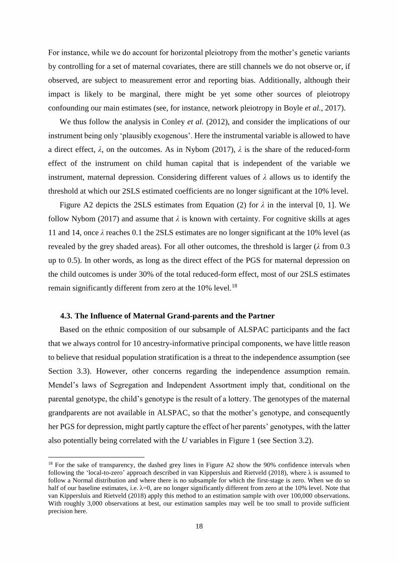
For instance, while we do account for horizontal pleiotropy from the mother’s genetic variants

by controlling for a set of maternal covariates, there are still channels we do not observe or, if

observed, are subject to measurement error and reporting bias. Additionally, although their

impact is likely to be marginal, there might be yet some other sources of pleiotropy

confounding our main estimates (see, for instance, network pleiotropy in Boyle et al., 2017).

We thus follow the analysis in Conley et al. (2012), and consider the implications of our

instrument being only ‘plausibly exogenous’. Here the instrumental variable is allowed to have

a direct effect, λ, on the outcomes. As in Nybom (2017), λ is the share of the reduced-form

effect of the instrument on child human capital that is independent of the variable we

instrument, maternal depression. Considering different values of λ allows us to identify the

threshold at which our 2SLS estimated coefficients are no longer significant at the 10% level.

Figure A2 depicts the 2SLS estimates from Equation (2) for λ in the interval [0, 1]. We

follow Nybom (2017) and assume that λ is known with certainty. For cognitive skills at ages

11 and 14, once λ reaches 0.1 the 2SLS estimates are no longer significant at the 10% level (as

revealed by the grey shaded areas). For all other outcomes, the threshold is larger (λ from 0.3

up to 0.5). In other words, as long as the direct effect of the PGS for maternal depression on

the child outcomes is under 30% of the total reduced-form effect, most of our 2SLS estimates

remain significantly different from zero at the 10% level.18

4.3. The Influence of Maternal Grand-parents and the Partner

Based on the ethnic composition of our subsample of ALSPAC participants and the fact

that we always control for 10 ancestry-informative principal components, we have little reason

to believe that residual population stratification is a threat to the independence assumption (see

Section 3.3). However, other concerns regarding the independence assumption remain.

Mendel’s laws of Segregation and Independent Assortment imply that, conditional on the

parental genotype, the child’s genotype is the result of a lottery. The genotypes of the maternal

grandparents are not available in ALSPAC, so that the mother’s genotype, and consequently

her PGS for depression, might partly capture the effect of her parents’ genotypes, with the latter

also potentially being correlated with the U variables in Figure 1 (see Section 3.2).

18 For the sake of transparency, the dashed grey lines in Figure A2 show the 90% confidence intervals when

following the ‘local-to-zero’ approach described in van Kippersluis and Rietveld (2018), where λ is assumed to

follow a Normal distribution and where there is no subsample for which the first-stage is zero. When we do so

half of our baseline estimates, i.e. λ=0, are no longer significantly different from zero at the 10% level. Note that

van Kippersluis and Rietveld (2018) apply this method to an estimation sample with over 100,000 observations.

With roughly 3,000 observations at best, our estimation samples may well be too small to provide sufficient

precision here.

19

While we cannot control for the genetic variants of the maternal grandparents, we do have

data on a set of grandparental traits: their education, social status, and a dummy for at least one

of the maternal grandparents having had a severe mental illness prior to the birth of the child.

The results controlling for these variables appear in Table A7. The 2SLS estimates are virtually

unchanged from those in the baseline. The F-statistics are slightly lower. This is unsurprising:

even though, after conditioning on the mother’s traits, none of the grandparental characteristics

is correlated with child human-capital, the mother having at least one parent with a history of

mental illness is positively and significantly associated with both our measure of maternal

depression and her PGS for depression.

We finally consider assortative matching between the child’s parents: depressed mothers

might choose their partners according to certain traits (depression itself, and/or other traits),

which may in turn affect child human capital. Our main specification, which includes a number

of the mother’s partner’s controls, partly addresses this. We can further show that these traits

(having a partner, partner’s working status and education) are not systematically explained by

the mother’s PGS for depression (see Table A4). While this alleviates concerns about cross-

trait assortative matching, mothers with a higher genetic risk of being depressed might be more

likely to have a depressed partner. We have information on the mother’s partner’s number of

depression episodes, measured at child ages 2, 4 and 6. While the unconditional correlation

between the partner’s depression and maternal depression is relatively high (0.44) and

significant, its correlation with the PGS for maternal depression is not statistically different

from zero (in both bivariate and multivariate analyses). Introducing partner’s depression makes

little difference to our main results: see Table A8.

4.4. Robustness Checks

4.4.1. The Measurement of Maternal Depression

We carry out a battery of robustness checks. We first show that our results hold with

different maternal-depression measures (the descriptive statistics of which appear in Table A9).

Our baseline count of reported depressive episodes between child ages 0 and 9 weights recent

and more-distant episodes equally, but those at younger child ages may matter more (as

children then have greater developmental plasticity and spend more time with their mothers).

Panels B and C of Table A10 however reveal larger estimates for more-recent depressive

episodes (although the estimated coefficients between these panels are not significantly

different from each other). The results continue to hold using only the number of episodes net

of post-partum depression (i.e. between child ages 2 and 9) in Panel D, and with a dummy for

20

any episode of depression in Panel E. Panel F considers a dummy for recent depression and

Panel G the average of the six maternal scores on the Edinburgh Postnatal Depression Scale

(EPDS) between child ages 0 and 8 (at child age 8 months and 2, 3, 5, 6 and 8 years). Although

the results continue to be of the same nature, the F-statistics are notably worse. The instrument

weakness here reveals that our PGS has greater predictive power when maternal depression is

measured over longer time periods and in a similar way to that in the GWAS meta-analysis

(the EPDS does not appear in Turley et al., 2018).

4.4.2. The Measurement of Non-Cognitive Skills

The SDQ measure of non-cognitive skills we use is reported by the mother. As depressed

mothers may over- or under-estimate their children’s non-cognitive skills (Del Bono et al.,

2020) we turn to teacher-reported SDQ (which is only available when the child was aged 11).

In the first column of Table A11, an additional episode of maternal depression continues to

reduce total SDQ with an effect size identical to that in Table 2.19 We also test for convergent

validity using the SMFQ (reported by the main carer) in columns (2) to (4) of Table A11: the

resulting estimates are not significantly different from those in the baseline (although that at

age 16 is statistically insignificant).

5. Conclusion

Social scientists are interested in causal phenomena, and research agendas are partly limited

to the analysis of variables that can be influenced, either directly or via policy intervention.

However, there are many variables and pathways that are either costly or impossible to

manipulate. We believe that it is possible to make causal statements about some of these latter

via the increasing availability of genetic data and recent developments in the fields of

Epidemiology and Molecular Genetics. This is the approach that we have taken here. However,

the use of genetic data as instruments is not a quick fix, as it comes with a number of quite-

stringent assumptions. We have here discussed a number of tests and tools that can be applied

in this empirical setting.

We illustrate how genetic data can be used to identify the effect of maternal depression on

children’s human capital, using data from a British birth-cohort study. We first show that

genetic variants, combined into a synthetic polygenic score, are a strong instrumental variable

19 Total SDQ can be split into two finer subscales: internalising SDQ (emotional health: the sum of ‘peer problems’

and ‘emotional problems’) and externalising SDQ (behavioural issues: the sum of ‘hyperactivity/inattention’ and

‘conduct problems’). Maternal depression produces worse outcomes for both internalising and externalising SDQ.

These results are available upon request.

21

for maternal depression. In 2SLS estimation, we then exploit the exogenous differences in

maternal depression resulting from the mother’s genes to identify its negative consequences on

the cognitive and non-cognitive outcomes of their adolescent children.

Our results suggest that fewer episodes of maternal depression will not only benefit

mothers, but also improve their children’s human capital. In turn, better cognitive and non-

cognitive skills in childhood are known to have positive returns on a variety of outcomes during

adulthood, such as income and labour-market experience (Heckman et al., 2006; Heckman et

al., 2018; Clark et al., 2018; Clark and Lepinteur, 2019). As revealed by the evaluation of the

Improving Access to Psychological Therapies programme in the UK in Clark (2018), the costs

of effective treatments for depression are extremely low compared to their expected benefits.

If treatment also produces positive spillovers on children, the benefit-cost ratio will be even

higher, making treatment more attractive.

However, as we compare depressed to not-depressed or less-depressed mothers using cross-

section data on adolescents, our results do not tell us how changes in depression (in particular,

due to its treatment) would affect children. Baranov et al. (2020) find only small long-term

effects on child development following the treatment of prenatally-depressed mothers in rural

Pakistan. The socio-economic, geographical and temporal contexts of our work and those in

Baranov et al. (2020) are of course dissimilar. More importantly, they look at mothers who

were already depressed pre-birth, whereas we consider a general sample of mothers, some of

whom experience episodes of depression after birth and some of whom do not. While we show

that the experience of maternal depression has large scarring effects on adolescent children, we

do not know how easy it is to erase these scars. Policies that aim to prevent depression, rather

than treat it once it occurs, may have a greater return from a societal perspective.

The use of polygenic scores as instrumental variables is a promising avenue for causal

inference in observational data. It is however important to keep in mind that the genetic

component of complex traits, such as mental health, is far from deterministic. The same

polygenic score can be found in individuals with a very wide range of values of the trait of

interest. This may reflect that the individual genetic architecture predicts outcomes partly via

individuals’ reactions to their environment. This opens the door to policy intervention: while

genes are fixed, the environment is not. Future research on which stressors are the most

important in this context will help advance our understanding of the sign and size of causal

relationships that can serve as inputs to public-policy debate.

22

References

Angrist, J. D., and Pischke, J. S. (2008). Mostly Harmless Econometrics: An Empiricist's

Companion. Princeton University Press.

Banerjee, S., Chatterji, P., and Lahiri, K. (2017). “Effects of psychiatric disorders on labor

market outcomes: A latent variable approach using multiple clinical indicators.” Health

Economics, 26, 184-205.

Baranov, V., Bhalotra, S., Biroli, P., and Maselko, J. (2020). “Maternal depression, women's

empowerment, and parental investment: Evidence from a randomized controlled trial.”

American Economic Review, 110, 824-59.

Benke, K. S., Nivard, M. G., Velders, F. P., Walters, R. K., Pappa, I., Scheet, P. A., ... and

Verhulst, F. C. (2014). “A genome-wide association meta-analysis of preschool

internalizing problems.” Journal of the American Academy of Child and Adolescent

Psychiatry, 53, 667-676.

Boef, A. G., Dekkers, O. M., and Le Cessie, S. (2015). “Mendelian randomization studies: a

review of the approaches used and the quality of reporting.” International Journal of

Epidemiology, 44, 496-511.

Boyd, A., Macleod, J., Henderson, J., Molloy, L., Ring, S., Golding, J., and Ness, A. (2013).

“Cohort profile: The “Children of the 90s”-The index offspring of the Avon longitudinal

study of parents and children.” International Journal of Epidemiology, 42, 111-127.

Boyle, E. A., Li, Y. I., and Pritchard, J. K. (2017). “An expanded view of complex traits: from

polygenic to omnigenic.” Cell, 169, 1177-1186.

Briole, S., Le Forner, H., and Lepinteur, A. (2020). “Children’s socio-emotional skills: Is there

a quantity–quality trade-off?” Labour Economics, 64,

https://doi.org/10.1016/j.labeco.2020.101811.

Bubonya, M., Cobb-Clark, D. A., and Wooden, M. (2017). “Mental health and productivity at

work: Does what you do matter?” Labour Economics, 46, 150-165.

23

Clark, A.E., D’Ambrosio, C., and Barazzetta, M. (2021). “Childhood circumstances and young

adult outcomes: The role of mothers’ financial problems”. Health Economics, 30, 342-357.

Clark, A.E., Flèche, S., Layard, R., Powdthavee, N., and Ward, G. (2018). The Origins of

Happiness: The Science of Well-being over the Life Course. Princeton University Press.

Clark, A.E., and Lepinteur, A. (2019). “The causes and consequences of early-adult

unemployment: Evidence from cohort data.” Journal of Economic Behavior &

Organization, 166, 107-124.

Clark, D. M. (2018). “Realizing the mass public benefit of evidence-based psychological

therapies: the IAPT program.” Annual Review of Clinical Psychology, 14, 159-183.

Conley, T. G., Hansen, C. B., and Rossi, P. E. (2012). “Plausibly exogenous.” Review of

Economics and Statistics, 94, 260-272.

Cunha, F., and Heckman, J. J. (2008). “Formulating, identifying and estimating the technology

of cognitive and noncognitive skill formation.” Journal of Human Resources, 43, 738-782.

Dahlen, H. M. (2016). “The impact of maternal depression on child academic and

socioemotional outcomes.” Economics of Education Review, 52, 77-90.

Davey Smith, G., and Hemani, G. (2014). “Mendelian randomization: Genetic anchors for

causal inference in epidemiological studies.” Human Molecular Genetics, 23, 89-98.

Davies, N. M., von Hinke Kessler Scholder, S., Farbmacher, H., Burgess, S., Windmeijer, F.,

and Smith, G. D. (2015). “The many weak instruments problem and Mendelian

randomization.” Statistics in Medicine, 34, 454-468.

Del Bono, E., Kinsler, J., and Pavan, R. (2020). Skill Formation and the Trouble with Child

Non-Cognitive Skill Measures. IZA Discussion Paper No. 13713.

Demange, P. A., Malanchini, M., Mallard, T. T., Biroli, P., Cox, S. R., Grotzinger, A. D., ...

and Corcoran, D. (2021). “Investigating the genetic architecture of non-cognitive skills

using GWAS-by-subtraction.” Nature Genetics, 53, 35-44.

24

DiPrete, T. A., Burik, C. A., and Koellinger, P. D. (2018). “Genetic instrumental variable

regression: Explaining socioeconomic and health outcomes in nonexperimental data.”

Proceedings of the National Academy of Sciences, 115, 4970-4979.

Flèche, S. (2017). Teacher Quality, Test-scores and Non-Cognitive Skills: Evidence from

Primary School Teachers in the UK. CEP Discussion Paper No. 1472.

Fletcher, J. (2013). “Adolescent depression and adult labor market outcomes.” Southern

Economic Journal, 80, 26-49.

Fraser, A., Macdonald-Wallis, C., Tilling, K., Boyd, A., Golding, J., Davey Smith, G., ... and

Ring, S. (2013). “Cohort profile: The Avon Longitudinal Study of Parents and Children:

ALSPAC mothers cohort”. International Journal of Epidemiology, 42, 97-110.

Goodman, R. (1997). “The Strengths and Difficulties Questionnaire: A research note.” Journal

of Child Psychology and Psychiatry, 38, 581-586.

Goodman, A., Lamping, D. L., and Ploubidis, G. B. (2010). “When to use broader internalising

and externalising subscales instead of the hypothesised five subscales on the Strengths and

Difficulties Questionnaire (SDQ): Data from British parents, teachers and children.”

Journal of Abnormal Child Psychology, 38, 1179-1191.

Goodman, S. H., Rouse, M. H., Connell, A. M., Broth, M. R., Hall, C. M., and Heyward, D.

(2011). “Maternal depression and child psychopathology: A meta-analytic review.” Clinical

Child and Family Psychology Review, 14, 1-27.

Gotlib, I., Goodman, S., and Humphreys, K. (2020). “Studying the Intergenerational

Transmission of Risk for Depression: Current Status and Future Directions.” Current

Directions in Psychological Science, 29, 174-179.

Gotlib, I. H., Lewinsohn, P. M., and Seeley, J. R. (1998). “Consequences of depression during

adolescence: Marital status and marital functioning in early adulthood.” Journal of

Abnormal Psychology, 107, 686-690.

Grogger, J., and Eide, E. (1995). “Changes in college skills and the rise in the college wage

premium.” Journal of Human Resources, 30, 280-310.

25

Hakulinen, C., Elovainio, M., Arffman, M., Lumme, S., Pirkola, S., Keskimäki, I., ... and

Böckerman, P. (2019). “Mental disorders and long‐term labour market outcomes:

Nationwide cohort study of 2,055,720 individuals.” Acta Psychiatrica Scandinavica, 140,

371-381.

Hansell, N. K., Halford, G. S., Andrews, G., Shum, D. H., Harris, S. E., Davies, G., ... and

Medland, S. E. (2015). “Genetic basis of a cognitive complexity metric”. PloS One, 10,

https://doi.org/10.1371/journal.pone.0123886.

Hanushek, E.A. and Kimko, D.D. (2000). “Schooling, labor-force quality and the growth of

nations.” American Economic Review, 90, 1184-1208.

Heckman, J. J., Stixrud, J., and Urzua, S. (2006). “The effects of cognitive and noncognitive

abilities on labor market outcomes and social behavior.” Journal of Labor Economics, 24,

411-482.

Heckman, J. J., Humphries, J. E., and Veramendi, G. (2018). “Returns to education: The causal

effects of education on earnings, health, and smoking.” Journal of Political Economy, 126,

197-246.

Hemani, G., Bowden, J., and Davey Smith, G. (2018). “Evaluating the potential role of

pleiotropy in Mendelian randomization studies.” Human Molecular Genetics, 27, 195-208.

Karlsson Linnér, R., Biroli, P., Kong, E., Meddens, S. F. W., Wedow, R., Fontana, M. A., ...

and Nivard, M. G. (2019). “Genome-wide association analyses of risk tolerance and risky

behaviors in over 1 million individuals identify hundreds of loci and shared genetic

influences.” Nature Genetics, 51, 245-257.

Kiernan, K. E., and Huerta, M. C. (2008). “Economic deprivation, maternal depression,

parenting and children's cognitive and emotional development in early childhood.” British

Journal of Sociology, 59, 783-806.

Koellinger, P. D., and De Vlaming, R. (2019). “Mendelian randomization: the challenge of

unobserved environmental confounds.” International Journal of Epidemiology, 48, 665-

671.

26

Kong, A., Thorleifsson, G., Frigge, M. L., Vilhjalmsson, B. J., Young, A. I., Thorgeirsson, T.

E., ... and Gudbjartsson, D. F. (2018). “The nature of nurture: effects of parental genotypes.”

Science, 359, 424-428.

Lawlor, D., Richmond, R., Warrington, N., McMahon, G., Smith, G. D., Bowden, J., and

Evans, D. M. (2017). “Using Mendelian randomization to determine causal effects of

maternal pregnancy (intrauterine) exposures on offspring outcomes: Sources of bias and

methods for assessing them.” Wellcome Open Research, 2,

https://doi.org/10.12688/wellcomeopenres.10567.1.

Lee, J. J., Wedow, R., Okbay, A., Kong, E., Maghzian, O., Zacher, M., ... & Fontana, M. A.

(2018). “Gene discovery and polygenic prediction from a genome-wide association study

of educational attainment in 1.1 million individuals.” Nature Genetics, 50, 1112-1121.

Middeldorp, C. M., Hammerschlag, A. R., Ouwens, K. G., Groen-Blokhuis, M. M., Pourcain,

B. S., Greven, C. U., ... and Vilor-Tejedor, N. (2016). “A genome-wide association meta-

analysis of attention-deficit/hyperactivity disorder symptoms in population-based pediatric

cohorts.” Journal of the American Academy of Child and Adolescent Psychiatry, 55, 896-

905.

Murnane, R.J., Singer, J.D., Willet, J.B., Kemple, J.J. and Olsen, R. (1991). Who Will Teach?

Policies that Matter. Cambridge, MA: Harvard University Press.

Nybom, M. (2017). “The distribution of lifetime earnings returns to college.” Journal of Labor

Economics, 35, 903-952.

O’Hara, M. W., and McCabe, J. E. (2013). “Postpartum depression: Current status and future

directions.” Annual Review of Clinical Psychology, 9, 379-407.

Okbay, A., Baselmans, B. M., De Neve, J. E., Turley, P., Nivard, M. G., Fontana, M. A., ...

and Gratten, J. (2016). “Genetic variants associated with subjective well-being, depressive

symptoms, and neuroticism identified through genome-wide analyses.” Nature Genetics,

48, 624-633.

27

Pappa, I., St Pourcain, B., Benke, K., Cavadino, A., Hakulinen, C., Nivard, M. G., ... and Evans,

D. M. (2016). “A genome‐wide approach to children's aggressive behavior: The EAGLE

consortium.” American Journal of Medical Genetics Part B: Neuropsychiatric Genetics,

171, 562-572.

Perry, C. D. (2008). “Does treating maternal depression improve child health management?

The case of pediatric asthma.” Journal of Health Economics, 27, 157-173.

Prince, M., Patel, V., Saxena, S., Maj, M., Maselko, J., Phillips, M.R., and Rahman, A. (2007).

“No health without mental health.” Lancet, 370, 859-877.

Rajagopal, V. M., Ganna, A., Coleman, J. R., Allegrini, A. G., Voloudakis, G., Grove, J., ...

and Schork, A. (2020). Genome-wide association study of school grades identifies a genetic

overlap between language ability, psychopathology and creativity. bioRxiv.

Smith, G. D., Lawlor, D. A., Harbord, R., Timpson, N., Day, I., and Ebrahim, S. (2007).

“Clustered environments and randomized genes: A fundamental distinction between

conventional and genetic epidemiology”. PLoS Medicine, 4, 1985-1992.

Stansfeld, S., Clark, C., Bebbington, P., King, M., Jenkins, R., and Hinchliffe, S. (2016).

“Chapter 2: Common mental disorders.” In S. McManus, P. Bebbington, R. Jenkins, and T.

Brugha (Eds.), Mental Health and Wellbeing in England: Adult Psychiatric Morbidity

Survey 2014 (pp. 37-68). Leeds: NHS Digital.

Taylor, A. E., Jones, H. J., Sallis, H., Euesden, J., Stergiakouli, E., Davies, N. M., ... & Tilling,

K. (2018). “Exploring the association of genetic factors with participation in the Avon

Longitudinal Study of Parents and Children.” International Journal of Epidemiology, 47,

1207-1216.

Turley, P., Walters, R. K., Maghzian, O., Okbay, A., Lee, J. J., Fontana, M. A., ... and

Magnusson, P. (2018). “Multi-trait analysis of genome-wide association summary statistics

using MTAG.” Nature Genetics, 50, 229-237.

Van Kerm, P. (2003). “Adaptive kernel density estimation”. Stata Journal, 3, 148-156.

Van Kippersluis, H., and Rietveld, C. A. (2018). “Pleiotropy-robust Mendelian

randomization.” International Journal of Epidemiology, 47, 1279-1288.

28

Von Hinke, S., Rice, N., and Tominey, E. (2019). Mental Health around Pregnancy and Child

Development from Early Childhood to Adolescence. IZA Discussion Paper No. 12544.

Von Hinke, S., Smith, G. D., Lawlor, D. A., Propper, C., and Windmeijer, F. (2016). “Genetic

markers as instrumental variables.” Journal of Health Economics, 45, 131-148.

Zhang, G., Bacelis, J., Lengyel, C., Teramo, K., Hallman, M., Helgeland, Ø., ... and Jacobsson,

B. (2015). “Assessing the causal relationship of maternal height on birth size and gestational

age at birth: a mendelian randomization analysis.” PLoS Medicine, 12,

10.1371/journal.pmed.1001865.

Zimmerman F., and Katon, W. (2005). “Socioeconomic status, depression disparities, and

financial strain: What lies behind the income-depression relationship?” Health Economics,

14, 1197-1215.

29

Figure 1: A Directed Acyclic Graph Illustrating the IV Setup and its Assumptions

Notes: The solid black lines depict the standard IV setup, where GM

D is a (vector of)

instrument(s) for a maternal trait DM and YC is the child-level outcome of interest. U is a set of

unobservable confounders of the trait-outcome association that should not be correlated with

GMD (the independence assumption, i.e. 𝜂 = 0). XM is a set of maternal traits that are influenced

by GMD through horizontal pleiotropy or other confounding pathways (e.g. genetic nurture) and

have an impact on YC, thus violating the exclusion restriction. The identification issues in the

bottom half of the figure reflect genetic inheritance (GCD and GC

Y are, respectively, the child’s

genetic variants for traits D and Y). Lines with arrows at the end represent causal relationships;

the line between GMD and U does not have an arrow and therefore reflects a correlational

relationship.

30

Figure 2: Maternal Depression and Child Human Capital:

2SLS Results with Different Sets of Covariates

Notes: The horizontal lines in each bar show the 90% confidence intervals. All of the dependent variables are

standardised. The child traits are the child’s gender, birth year and birth-order dummies. The mother’s traits are

the child’s number of siblings in the household, the age of the mother at birth of the cohort member, dummies

for the mother having at least an A-level, working, having a partner, having a partner with at least an A-level,

and having a working partner, and dummies for banded household income. All regressions using test-scores as

the dependent variable include school and school-year fixed effects. The Cragg-Donald Wald F-statistics for

weak identification, going from the “No traits” specification to the “All traits” specification, are the following:

for KS2, 15.5, 16.0, 13.0, 14.0; for KS3, 20.9, 20.7, 18.8, 19.5; for KS4, 22.8, 22.2, 20.6, 21.2; for SDQ11, 23.8,

23.0, 20.6, 21.0; for SDQ13, 22.1, 21.4, 21.1, 20.8; for SDQ16, 9.7, 9.2, 8.3, 8.1. *** p<0.01, ** p<0.05, * p<0.1.

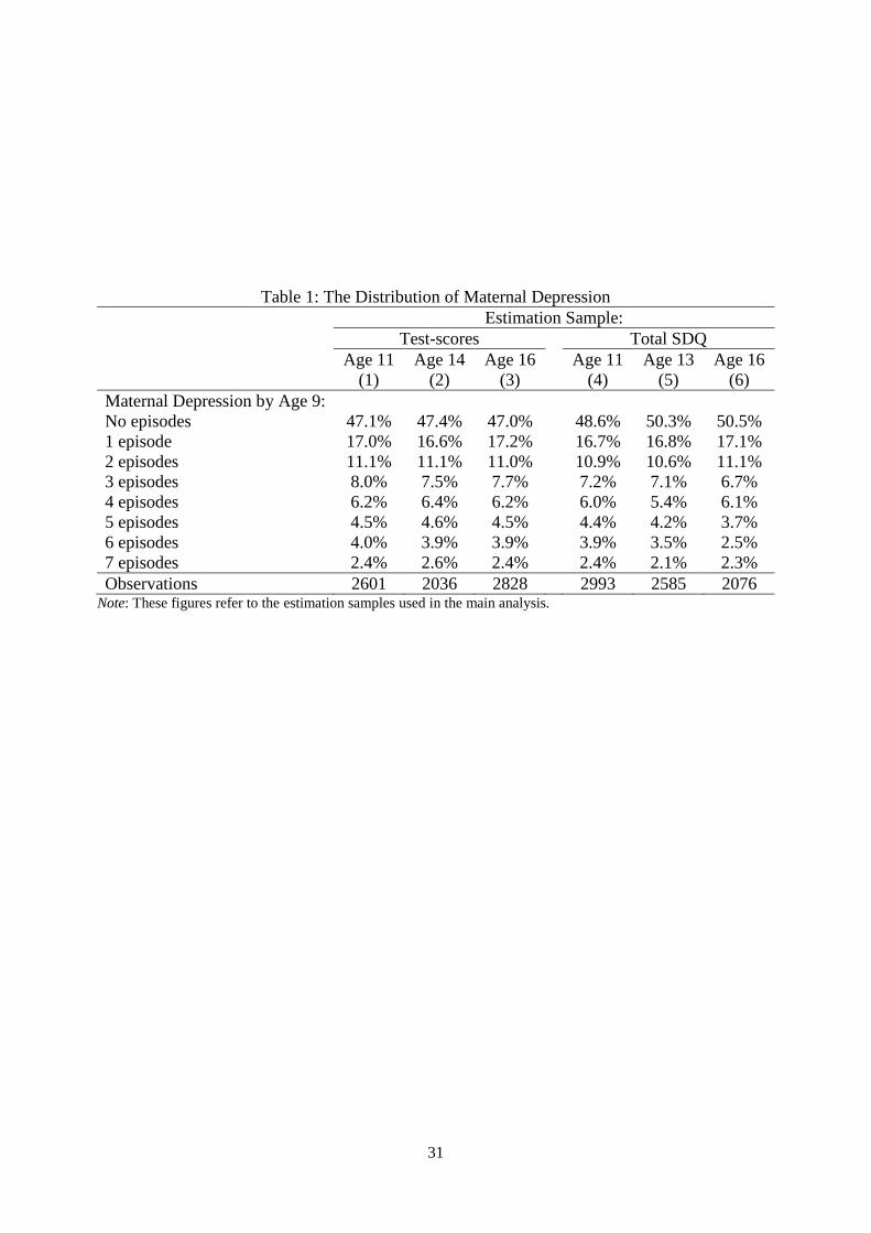
31

Table 1: The Distribution of Maternal Depression

Estimation Sample:

Test-scores Total SDQ

Age 11 Age 14 Age 16 Age 11 Age 13 Age 16

(1) (2) (3) (4) (5) (6)

Maternal Depression by Age 9:

No episodes 47.1% 47.4% 47.0% 48.6% 50.3% 50.5%

1 episode 17.0% 16.6% 17.2% 16.7% 16.8% 17.1%

2 episodes 11.1% 11.1% 11.0% 10.9% 10.6% 11.1%

3 episodes 8.0% 7.5% 7.7% 7.2% 7.1% 6.7%

4 episodes 6.2% 6.4% 6.2% 6.0% 5.4% 6.1%

5 episodes 4.5% 4.6% 4.5% 4.4% 4.2% 3.7%

6 episodes 4.0% 3.9% 3.9% 3.9% 3.5% 2.5%

7 episodes 2.4% 2.6% 2.4% 2.4% 2.1% 2.3%

Observations 2601 2036 2828 2993 2585 2076 Note: These figures refer to the estimation samples used in the main analysis.

32

Table 2: Maternal Depression and Child Human Capital: OLS and 2SLS Results

Test-scores

Age 11 Age 14 Age 16

OLS 2SLS OLS 2SLS OLS 2SLS

(1) (2) (3) (4) (5) (6)

Maternal Depression -0.018* -0.222* -0.031*** -0.178* -0.016* -0.273***

(0.010) (0.120) (0.010) (0.097) (0.009) (0.102)

First Stage:

Mother's PGS 0.158*** 0.205*** 0.179***

(0.042) (0.046) (0.039)

F-statistics 14.1 19.5 21.2

Observations 2601 2601 2036 2036 2828 2828

Total SDQ

Age 11 Age 13 Age 16

OLS 2SLS OLS 2SLS OLS 2SLS

(1) (2) (3) (4) (5) (6)

Maternal Depression -0.100*** -0.390*** -0.087*** -0.421*** -0.083*** -0.531**

(0.009) (0.128) (0.010) (0.136) (0.012) (0.245)

First Stage:

Mother's PGS 0.160*** 0.167*** 0.114***

(0.035) (0.037) (0.040)

F-statistics 20.9 20.8 8.1

Observations 2993 2993 2585 2585 2076 2076 Notes: Standard errors appear in parentheses. All dependent variables are standardised. Maternal depression is the number

of episodes of depression reported by the mother from the birth of the child to the child’s ninth birthday. The controls are:

the child’s gender, birth year, birth order, number of siblings, the age of the mother at the birth of the child; dummies for

the mother having at least an A-level, being employed, having a partner, having a partner with at least an A-level, having

an employed partner, dummies for banded household income and ancestry-informative principal components. All

regressions using test-scores as the dependent variable include school and school-year fixed effects. The reported F-

statistics are those for the Cragg-Donald Wald weak-identification test. *** p<0.01, ** p<0.05, * p<0.1.

33

Table 3: Addressing Genetic Inheritance for Maternal Depression and Child Human Capital: 2SLS results

Test-scores

Age 11 Age 14 Age 16

(1) (2) (3) (4) (5) (6) (7) (8) (9) (10) (11) (12)

Maternal Depression -0.222* -0.192 -0.238* -0.225* -0.178* -0.164* -0.182** -0.177** -0.273*** -0.255** -0.294*** -0.288***

(0.120) (0.117) (0.123) (0.121) (0.097) (0.096) (0.089) (0.089) (0.102) (0.100) (0.106) (0.105)

Child PGS: 0.071*** 0.072*** 0.047** 0.047** 0.061*** 0.062***

Cognitive Skills (0.020) (0.021) (0.022) (0.022) (0.020) (0.020)

Child PGS: 0.005 0.012 0.002 0.006 0.009 0.014

Depression (0.022) (0.021) (0.021) (0.021) (0.021) (0.021)

F-statistics 14.1 13.9 13.7 13.7 19.5 19.2 23.0 22.9 21.2 21.3 20.3 20.4

Observations 2601 2601 2601 2601 2036 2036 2036 2036 2828 2828 2828 2828

Total SDQ

Age 11 Age 13 Age 16

(1) (2) (3) (4) (5) (6) (7) (8) (9) (10) (11) (12)

Maternal Depression -0.390*** -0.391*** -0.295** -0.296** -0.421*** -0.421*** -0.384*** -0.383*** -0.531** -0.529** -0.478* -0.482*

(0.128) (0.128) (0.124) (0.124) (0.136) (0.136) (0.127) (0.127) (0.245) (0.244) (0.249) (0.250)

Child PGS: 0.044** 0.039* 0.058** 0.056** 0.077** 0.074**

Non-Cognitive Skills (0.022) (0.021) (0.025) (0.024) (0.031) (0.031)

Child PGS: -0.036* -0.036* -0.015 -0.015 -0.014 -0.013

Depression (0.022) (0.022) (0.024) (0.024) (0.031) (0.031)

F-statistics 20.9 20.9 19.5 19.4 20.8 20.8 22.4 22.4 8.1 8.1 7.1 7.0

Observations 2993 2993 2993 2993 2585 2585 2585 2585 2076 2076 2076 2076 Notes: Standard errors are in parentheses. All dependent variables are standardised. Maternal depression is the number of episodes of depression reported by the mother from the birth of

the child to the child’s ninth birthday. The controls are: the child’s gender, birth year, birth order, number of siblings, the age of the mother at the birth of the child; dummies for the mother

having at least an A-level, being employed, having a partner, having a partner with at least an A-level, having an employed partner, dummies for banded household income and ancestry-

informative principal components. All regressions using test-scores as the dependent variable include school and school-year fixed effects. The reported F-statistics are those for the Cragg-

Donald Wald weak-identification test. *** p<0.01, ** p<0.05, * p<0.1.

34

Appendix A: Additional Figures and Tables

Figure A1: The Distribution of Test-scores and Total SDQ

Notes: Each figure refers to one of our estimation samples. The test-scores at age 11, 14 and 16 respectively refer

to the Key-Stage 2 average score, Key-Stage 3 average score and GCSE total score. The densities are plotted

using an adaptive-kernel (see Van Kerm, 2003, for the technical details).

35

Figure A2: Plausible Exogeneity and Pleiotropy-robust MR

Notes: Lambda represents the share of the reduced-form effect of the instrument on the outcome that

is independent of maternal depression. The black line is the 2SLS point estimate of maternal

depression for different values of lambda; the grey solid area represents 90% confidence intervals

using the Nybom (2017) approach, while the grey dashed lines are the 90% confidence intervals

following van Kippersluis and Rietveld (2018).

36

Table A1: Strengths and Difficulties Questionnaire (SDQ)

Please think about this child’s behaviour over the last 6 months if you can

This child: Not True Somewhat

True

Certainly

True

1. Is considerate of other people’s feelings [PS] 2 1 0

2. Is restless, overactive, cannot stay still for long

[H]

0 1 2

3. Often complains of headaches, stomach-aches or

sickness [E]

0 1 2

4. Shares readily with other children, for example

toys, treats, pencils [PS]

2 1 0

5. Often loses temper [B] 0 1 2

6. Is rather solitary, prefers to play alone [P] 0 1 2

7. Is generally well behaved, usually does what

adults request [B]

2 1 0

8. Has many worries or often seems worried [E] 0 1 2

9. Is helpful if someone is hurt, upset or feeling ill

[PS]

2 1 0

10. Is constantly fidgeting or squirming [H] 0 1 2

11. Has at least one good friend [P] 2 1 0

12. Often fights with other children or bullies them

[B]

0 1 2

13. Is often unhappy, depressed or tearful [E] 0 1 2

14. Is generally liked by other children [P] 2 1 0

15. Is easily distracted, concentration wanders [H] 0 1 2

16. Is nervous or clingy in new situations, easily

loses confidence [E]

0 1 2

17. Is kind to younger children [PS] 2 1 0

18. Often lies or cheats [B] 0 1 2

19. Is picked on or bullied by other children [P] 0 1 2

20. Often volunteers to help others (parents,

teachers, other children) [PS]

2 1 0

21. Thinks things out before acting [H] 2 1 0

22. Steals from home, school or elsewhere [B] 0 1 2

23. Gets along better with adults than with other

children [P]

0 1 2

24. Has many fears, is easily scared [E] 0 1 2

25. Has a good attention span, sees chores or

homework through to the end [H]

2 1 0

Notes: [E], [B], [H], [P] and [PS] refer respectively to the following dimensions of the SDQ: “Emotional health”,

“Behaviour problems”, “Hyperactivity/inattention”, “Peer relationship problems” and “Pro-social behaviour”.

Internalising SDQ is the sum of the “Emotional health” and “Peer relation problems” scores, and externalising SDQ the

sum of the “Hyperactivity/inattention” and “Behaviour problems” scores. Total SDQ is the sum of internalising and

externalising SDQ.

37

Table A2: Descriptive Statistics: Cognitive-Skills Estimation Samples

Estimation Samples:

Test-scores (age 11)

2601 observations

Test-scores (age 14)

2036 observations

Test-scores (age 16)

2828 observations

Mean SD Min Max Mean SD Min Max Mean SD Min Max

Cohort member characteristics:

KS2 average score (fine-grading) 28.76 3.48 15 35

KS3 average score (fine-grading) 37.33 5.65 17 49

GCSE total score 445.48 132.63 0 1171

Female 0.51 0 1 0.52 0 1 0.51 0 1

Birth year:

1991 0.36 0 1 0.43 0 1 0.36 0 1

1992 0.63 0 1 0.57 0 1 0.64 0 1

1993 0.01 0 1 0.00 0 0 0.01 0 1

Birth order:

1st-born 0.46 0 1 0.45 0 1 0.46 0 1

2nd-born 0.37 0 1 0.38 0 1 0.37 0 1

3rd-born 0.14 0 1 0.13 0 1 0.14 0 1

4th-born or higher 0.03 0 1 0.03 0 1 0.03 0 1

Mother and family characteristics:

No. of episodes of maternal depression 1.50 1.94 0 7 1.51 1.96 0 7 1.50 1.94 0 7

Employed mother 0.74 0 1 0.74 0 1 0.73 0 1

Mother has an A-level or above 0.33 0 1 0.33 0 1 0.35 0 1

Age of the mother at child's birth 29.29 4.23 18 44 29.29 4.23 18 44 29.43 4.28 18 44

Presence of partner 0.94 0 1 0.94 0 1 0.94 0 1

Employed partner 0.89 0 1 0.89 0 1 0.88 0 1

Partner has an A-level or above 0.47 0 1 0.47 0 1 0.49 0 1

Number of siblings 2.29 0.77 0 6 2.29 0.77 0 6 2.28 0.76 0 6

Average family take-home income per week:

<£100 0.01 0 1 0.01 0 1 0.01 0 1

£100-£199 0.07 0 1 0.07 0 1 0.07 0 1

£200-£299 0.16 0 1 0.16 0 1 0.15 0 1

£300-£399 0.20 0 1 0.21 0 1 0.20 0 1

£400+ 0.47 0 1 0.46 0 1 0.48 0 1

Do not know 0.05 0 1 0.05 0 1 0.05 0 1

Missing 0.04 0 1 0.04 0 1 0.04 0 1 Note: These figures refer to our estimation samples.

38

Table A3: Descriptive Statistics: Non-Cognitive Skills Estimation Samples

Estimation Samples:

Total SDQ (age 11)

2993 observations

Total SDQ (age 13)

2585 observations

Total SDQ (age 16)

2076 observations

Mean SD Min Max Mean SD Min Max Mean SD Min Max

Cohort member characteristics:

Total SDQ 33.79 4.85 6 40 33.86 4.55 10 40 34.55 4.26 13 40

Female 0.50 0 1 0.50 0 1 0.53 0 1

Birth year:

1991 0.36 0 1 0.36 0 1 0.35 0 1

1992 0.63 0 1 0.63 0 1 0.64 0 1

1993 0.01 0 1 0.01 0 1 0.01 0 1

Birth order:

1st-born 0.47 0 1 0.47 0 1 0.48 0 1

2nd-born 0.37 0 1 0.37 0 1 0.37 0 1

3rd-born 0.13 0 1 0.13 0 1 0.12 0 1

4th-born or more 0.03 0 1 0.03 0 1 0.02 0 1

Mother and family characteristics:

No. of episode of maternal depression 1.46 1.94 0 7 1.37 1.88 0 7 1.33 1.84 0 7

Employed mother 0.73 0 1 0.74 0 1 0.74 0 1

Mother has an A-level or more 0.39 0 1 0.41 0 1 0.44 0 1

Age of the mother at child's birth 29.59 4.27 18 44 29.63 4.24 18 43 29.77 4.26 18 43

Presence of partner 0.94 0 1 0.94 0 1 0.95 0 1

Employed partner 0.89 0 1 0.89 0 1 0.90 0 1

Partner has an A-level or above 0.53 0 1 0.54 0 1 0.56 0 1

Number of siblings 2.27 0.76 0 6 2.26 0.75 0 6 2.25 0.74 0 6

Average family take-home income per week:

<£100 0.01 0 1 0.01 0 1 0.01 0 1

£100-£199 0.06 0 1 0.06 0 1 0.05 0 1

£200-£299 0.14 0 1 0.13 0 1 0.13 0 1

£300-£399 0.19 0 1 0.19 0 1 0.17 0 1

£400+ 0.51 0 1 0.53 0 1 0.55 0 1

Do not know 0.05 0 1 0.04 0 1 0.04 0 1

Missing 0.04 0 1 0.04 0 1 0.04 0 1 Note: These figures refer to our estimation samples.

39

Table A4: The PGS for Maternal Depression and Maternal Traits: Bivariate Associations

PGS for Maternal Depression

Maternal Traits:

Maternal Depression [0-7] 0.177***

(0.035)

Mother is Employed -0.007

(0.008)

Mother has at least an A-level 0.003

(0.009)

Age at Birth of CM 0.066

(0.076)

Mother has a Partner -0.005

(0.004)

Working Partner+ 0.002

(0.004)

Partner has at least an A-level 0.012

(0.009)

Number of Siblings 0.013

(0.014)

Family Income above the Median+ -0.013

(0.009) Notes: Each cell reports the estimate and standard errors (in parentheses) of separate

bivariate associations between the PGS for maternal depression and various maternal

traits. The bivariate regressions are based on the observations coming from our largest

estimation sample (the one for which the SDQ at age 11 is not missing: 2993

observations). Using our five other estimation samples produces similar estimates. + indicates that we excluded the missing values of the maternal traits from the

estimation sample (including the missing values and introducing a missing-indicator

flag produces similar estimates). *** p<0.01, ** p<0.05, * p<0.1.

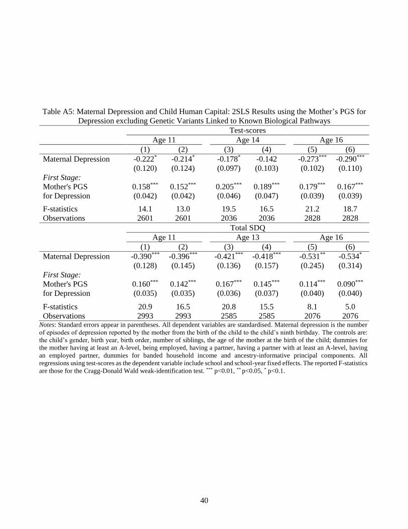
40

Table A5: Maternal Depression and Child Human Capital: 2SLS Results using the Mother’s PGS for

Depression excluding Genetic Variants Linked to Known Biological Pathways

Test-scores

Age 11 Age 14 Age 16

(1) (2) (3) (4) (5) (6)

Maternal Depression -0.222* -0.214* -0.178* -0.142 -0.273*** -0.290***

(0.120) (0.124) (0.097) (0.103) (0.102) (0.110)

First Stage:

Mother's PGS 0.158*** 0.152*** 0.205*** 0.189*** 0.179*** 0.167***

for Depression (0.042) (0.042) (0.046) (0.047) (0.039) (0.039)

F-statistics 14.1 13.0 19.5 16.5 21.2 18.7

Observations 2601 2601 2036 2036 2828 2828

Total SDQ

Age 11 Age 13 Age 16

(1) (2) (3) (4) (5) (6)

Maternal Depression -0.390*** -0.396*** -0.421*** -0.418*** -0.531** -0.534*

(0.128) (0.145) (0.136) (0.157) (0.245) (0.314)

First Stage:

Mother's PGS 0.160*** 0.142*** 0.167*** 0.145*** 0.114*** 0.090***

for Depression (0.035) (0.035) (0.036) (0.037) (0.040) (0.040)

F-statistics 20.9 16.5 20.8 15.5 8.1 5.0

Observations 2993 2993 2585 2585 2076 2076 Notes: Standard errors appear in parentheses. All dependent variables are standardised. Maternal depression is the number

of episodes of depression reported by the mother from the birth of the child to the child’s ninth birthday. The controls are:

the child’s gender, birth year, birth order, number of siblings, the age of the mother at the birth of the child; dummies for

the mother having at least an A-level, being employed, having a partner, having a partner with at least an A-level, having

an employed partner, dummies for banded household income and ancestry-informative principal components. All

regressions using test-scores as the dependent variable include school and school-year fixed effects. The reported F-statistics

are those for the Cragg-Donald Wald weak-identification test. *** p<0.01, ** p<0.05, * p<0.1.

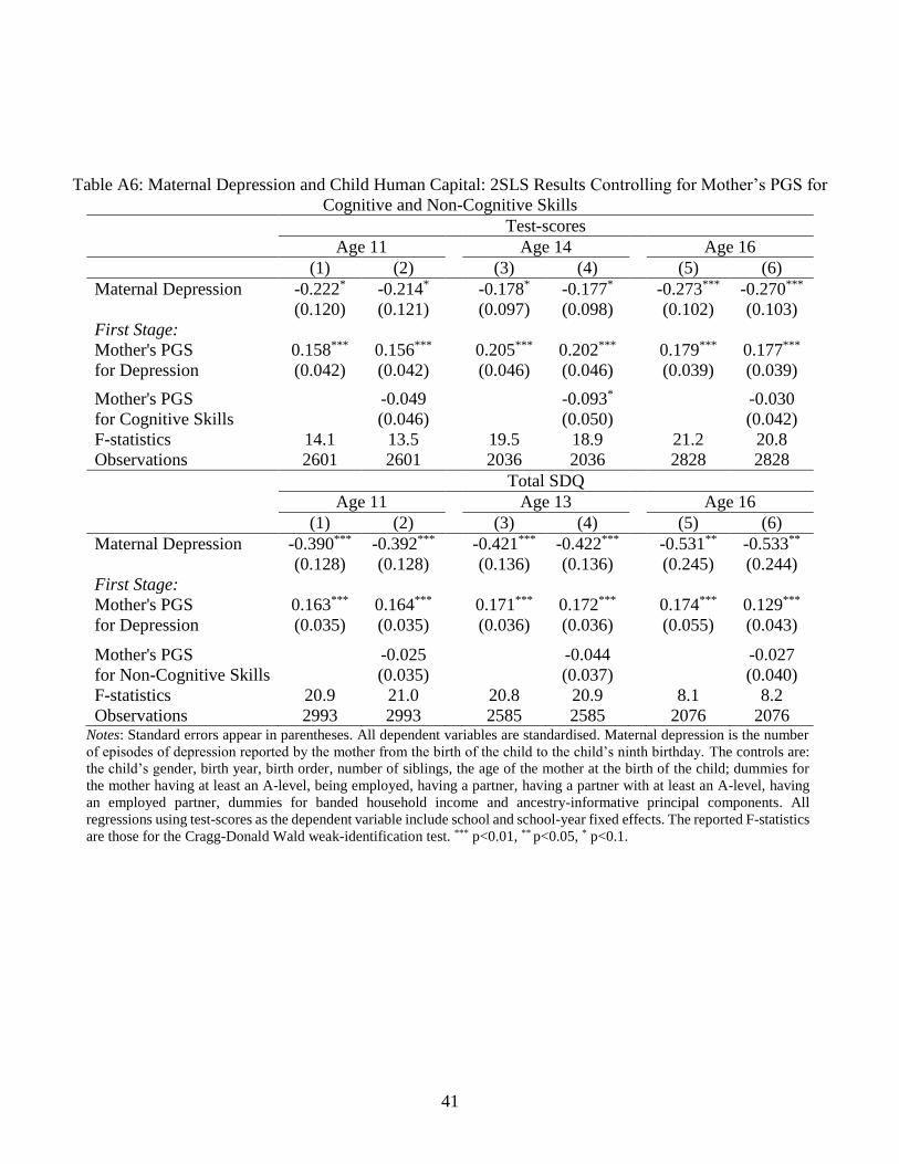
41

Table A6: Maternal Depression and Child Human Capital: 2SLS Results Controlling for Mother’s PGS for

Cognitive and Non-Cognitive Skills

Test-scores

Age 11 Age 14 Age 16

(1) (2) (3) (4) (5) (6)

Maternal Depression -0.222* -0.214* -0.178* -0.177* -0.273*** -0.270***

(0.120) (0.121) (0.097) (0.098) (0.102) (0.103)

First Stage:

Mother's PGS 0.158*** 0.156*** 0.205*** 0.202*** 0.179*** 0.177***

for Depression (0.042) (0.042) (0.046) (0.046) (0.039) (0.039)

Mother's PGS -0.049 -0.093* -0.030

for Cognitive Skills (0.046) (0.050) (0.042)

F-statistics 14.1 13.5 19.5 18.9 21.2 20.8

Observations 2601 2601 2036 2036 2828 2828

Total SDQ

Age 11 Age 13 Age 16

(1) (2) (3) (4) (5) (6)

Maternal Depression -0.390*** -0.392*** -0.421*** -0.422*** -0.531** -0.533**

(0.128) (0.128) (0.136) (0.136) (0.245) (0.244)

First Stage:

Mother's PGS 0.163*** 0.164*** 0.171*** 0.172*** 0.174*** 0.129***

for Depression (0.035) (0.035) (0.036) (0.036) (0.055) (0.043)

Mother's PGS -0.025 -0.044 -0.027

for Non-Cognitive Skills (0.035) (0.037) (0.040)

F-statistics 20.9 21.0 20.8 20.9 8.1 8.2

Observations 2993 2993 2585 2585 2076 2076 Notes: Standard errors appear in parentheses. All dependent variables are standardised. Maternal depression is the number

of episodes of depression reported by the mother from the birth of the child to the child’s ninth birthday. The controls are:

the child’s gender, birth year, birth order, number of siblings, the age of the mother at the birth of the child; dummies for

the mother having at least an A-level, being employed, having a partner, having a partner with at least an A-level, having

an employed partner, dummies for banded household income and ancestry-informative principal components. All

regressions using test-scores as the dependent variable include school and school-year fixed effects. The reported F-statistics

are those for the Cragg-Donald Wald weak-identification test. *** p<0.01, ** p<0.05, * p<0.1.

42

Table A7: Maternal Depression and Child Human Capital: 2SLS Results Controlling for Grandparental

Characteristics

Test-scores Total SDQ

Age 11 Age 14 Age 16 Age 11 Age 13 Age 16

(1) (2) (3) (4) (5) (6)

Maternal Depression -0.255* -0.186* -0.296*** -0.385*** -0.437*** -0.525*

(0.132) (0.100) (0.112) (0.138) (0.147) (0.273)

First Stage:

Mother's PGS 0.146*** 0.196*** 0.164*** 0.147*** 0.158*** 0.102**

(0.042) (0.047) (0.039) (0.035) (0.037) (0.040)

F-statistics 11.8 17.5 17.7 17.6 18.2 6.4

Observations 2601 2036 2828 2993 2585 2076 Notes: Standard errors are in parentheses. All dependent variables are standardised. Maternal depression is the

number of episodes of depression reported by the mother from the birth of the child to the child’s ninth birthday. The

controls are: the child’s gender, birth year, birth order, number of siblings, the age of the mother at the birth of the

child; dummies for the mother having at least an A-level, being employed, having a partner, having a partner with at

least an A-level, having an employed partner, dummies for banded household income and ancestry-informative

principal components. The regressions also include the following grandparental characteristics: dummies for the

mother having at least one parent who had a mental illness before the birth of the child and the highest diploma

obtained by the maternal grandmother and grandfather, and a social-status index for the maternal grandmother and

grandfather. All of the regressions using test-scores as the dependent variable include school and school-year fixed

effects. The reported F-statistics are those for the Cragg-Donald Wald weak-identification test. *** p<0.01, ** p<0.05, * p<0.1.

Table A8: Maternal Depression and Child Human Capital: 2SLS Results Controlling for Partner’s Depression

Test-scores Total SDQ

Age 11 Age 14 Age 16 Age 11 Age 13 Age 16

(1) (2) (3) (4) (5) (6)

Maternal Depression -0.240* -0.187* -0.297*** -0.406*** -0.436*** -0.566**

(0.129) (0.102) (0.113) (0.136) (0.143) (0.270)

First Stage:

Mother's PGS 0.148*** 0.195*** 0.163*** 0.151*** 0.160*** 0.105***

(0.040) (0.044) (0.037) (0.033) (0.035) (0.039)

Partner’s Depression 0.965*** 0.963*** 0.942*** 0.912*** 0.859*** 0.873***

(0.068) (0.073) (0.062) (0.056) (0.060) (0.066)

F-statistics 13.4 19.3 19.3 20.3 20.4 7.4

Observations 2601 2036 2828 2993 2585 2076 Notes: Standard errors appear in parentheses. All dependent variables are standardised. Maternal depression is the

number of episodes of depression reported by the mother from the birth of the child to the child’s ninth birthday. The

controls are: the child’s gender, birth year, birth order, number of siblings, the age of the mother at the birth of the

child; dummies for the mother having at least an A-level, being employed, having a partner, having a partner with at

least an A-level, having an employed partner, dummies for banded household income and ancestry-informative

principal components. All regressions using test-scores as the dependent variable include school and school-year

fixed effects. The reported F-statistics are those for the Cragg-Donald Wald weak-identification test. *** p<0.01, **

p<0.05, * p<0.1.

43

Table A9: Descriptive Statistics: Alternative Measures of Maternal Depression

Mean SD Min Max

Estimation Sample: Test-scores (age 11)

No. of depressive episodes between child age 0 and 5 1.06 1.44 0 5

No. of depressive episodes between child age 5 and 9 0.44 0.70 0 2

No. of depressive episodes between child age 2 and 9 1.25 1.70 0 6

Had at least one episode of depression 0.48 0 1

Recent depression 0.24 0 1

Mean EPDS 5.60 3.80 0 24.33

Estimation Sample: Test-scores (age 14)

No. of depressive episodes between child age 0 and 5 1.08 1.46 0 5

No. of depressive episodes between child age 5 and 9 0.43 0.70 0 2

No. of depressive episodes between child age 2 and 9 1.25 1.71 0 6

Had at least one episode of depression 0.48 0 1

Recent depression 0.23 0 1

Mean EPDS 5.62 3.84 0 24

Estimation Sample: Test-scores (age 16)

No. of depressive episodes between child age 0 and 5 1.06 1.44 0 5

No. of depressive episodes between child age 5 and 9 0.44 0.70 0 2

No. of depressive episodes between child age 2 and 9 1.25 1.70 0 6

Had at least one episode of depression 0.48 0 1

Recent depression 0.24 0 1

Mean EPDS 5.56 3.76 0 24

Estimation Sample: Total SDQ (age 11)

No. of depressive episodes between child age 0 and 5 1.03 1.44 0 5

No. of depressive episodes between child age 5 and 9 0.43 0.70 0 2

No. of depressive episodes between child age 2 and 9 1.21 1.70 0 6

Had at least one episode of depression 0.47 0 1

Recent depression 0.23 0 1

Mean EPDS 5.47 3.72 0 24

Estimation Sample: Total SDQ (age 13)

No. of depressive episodes between child age 0 and 5 0.97 1.40 0 5

No. of depressive episodes between child age 5 and 9 0.40 0.68 0 2

No. of depressive episodes between child age 2 and 9 1.14 1.66 0 6

Had at least one episode of depression 0.45 0 1

Recent depression 0.22 0 1

Mean EPDS 5.30 3.60 0 24

Estimation Sample: Total SDQ (age 16)

No. of depressive episodes between child age 0 and 5 0.95 1.38 0 5

No. of depressive episodes between child age 5 and 9 0.39 0.66 0 2

No. of depressive episodes between child age 2 and 9 1.10 1.62 0 6

Had at least one episode of depression 0.21 0 1

Recent depression 0.44 0 1

Mean EPDS 5.27 3.54 0 24 Note: These figures refer to the estimation samples used in Table A10.

44

Table A10: Alternative Measures of Maternal Depression and Child Human Capital: 2SLS results

Test-scores Total SDQ

Age 11 Age 14 Age 16 Age 11 Age 13 Age 16

(1) (2) (3) (4) (5) (6)

Panel A (Main estimates from Table 2)

No. of depressive episodes -0.227* -0.179* -0.284*** -0.394*** -0.416*** -0.498**

between child ages 0 and 9 (0.118) (0.093) (0.102) (0.125) (0.132) (0.211)

F-statistics 14.8 21.3 21.8 22.1 22.2 10.3

Observations 2601 2036 2828 2993 2585 2076

Panel B

No. of depressive episodes -0.273** -0.223* -0.364*** -0.512*** -0.579*** -0.597**

up to child’s 5th birthday (0.139) (0.115) (0.130) (0.162) (0.187) (0.244)

F-statistics 18.2 24.7 23.7 23.5 20.5 12.5

Observations 2601 2036 2828 2993 2585 2076

Panel C

No. of depressive episodes -0.681* -0.545* -0.777** -1.019*** -0.969*** -1.750

between child ages 5 and 9 (0.409) (0.320) (0.328) (0.375) (0.335) (1.112)

F-statistics 6.0 8.4 10.4 12.4 15.6 3.0

Observations 2601 2036 2828 2993 2585 2076

Panel D

No. of depressive episodes -0.282* -0.218* -0.345*** -0.468*** -0.475*** -0.572**

between child ages 2 and 9 (0.148) (0.114) (0.126) (0.151) (0.152) (0.245)

F-statistics 12.6 18.8 19.1 20.4 21.9 10.0

Observations 2601 2036 2828 2993 2585 2076

Panel E

Had at least one episode -0.948* -0.843* -1.234*** -1.555*** -1.631*** -1.520**

of depression (dummy) (0.502) (0.457) (0.463) (0.502) (0.532) (0.610)

F-statistics 12.6 14.6 17.0 20.9 20.2 14.8

Observations 2601 2036 2828 2993 2585 2076

Panel F

Recent depression (dummy) -3.218 -1.972 -2.565** -3.162** -2.826** -7.374

(2.759) (1.339) (1.283) (1.358) (1.107) (7.789)

F-statistics 1.6 3.8 5.5 7.1 9.9 0.9

Observations 2601 2036 2828 2993 2585 2076

Panel G

Average EPDS -0.889 -0.583* -1.038** -1.220*** -0.961*** -2.048

(0.568) (0.336) (0.485) (0.443) (0.315) (1.394)

F-statistics 3.7 7.1 6.4 9.1 15.2 2.2

Observations 2559 1998 2783 2947 2548 2053 Notes: Standard errors appear in parentheses. All dependent variables are standardised. All non-binary measures of maternal depression are

standardised. The controls are: the child’s gender, birth year, birth order, number of siblings, the age of the mother at the birth of the child;

dummies for the mother having at least an A-level, being employed, having a partner, having a partner with at least an A-level, having an

employed partner, dummies for banded household income and ancestry-informative principal components. All of the regressions with test-

scores as the dependent variables include school and school-year fixed effects. The difference in observations in the sixth panel is due to

missing values for the EPDS (Edinburgh Postnatal Depression Score) when the cohort member was eight years old. The reported F-statistics

are those for the Cragg-Donald Wald weak-identification test. *** p<0.01, ** p<0.05, * p<0.1.

45

Table A11: Maternal Depression and Children’s Non-Cognitive Skills: Validity Tests - 2SLS Results

Total SDQ

(Teacher reported)

SMFQ

(Main-carer reported)

Age 11 Age 11 Age 13 Age 16

(1) (2) (3) (4)

Maternal Depression -0.332** -0.399*** -0.362*** -0.130

(0.165) (0.128) (0.133) (0.188)

First Stage:

Mother's PGS 0.172*** 0.160*** 0.163*** 0.116***

(0.048) (0.035) (0.037) (0.041)

F-statistics 12.6 20.9 19.4 8.1

Observations 1559 2993 2558 2015 Notes: Standard errors are in parentheses. All dependent variables are standardised. SMFQ takes on

integer values from 0 to 26. The mean values (standard deviations) at ages 11, 13 and 16 are 23.8 (3.1),

23.9 (3.1) and 24.2 (3.0). Teacher-reported total SDQ at age 11 is on the same scale as carer-reported

total SDQ, with mean (standard deviation) of 35.5 (5.1). Maternal depression is the number of episodes

of depression reported by the mother from the birth of the child to the child’s ninth birthday. The controls

are: the child’s gender, birth year, birth order, number of siblings, the age of the mother at the birth of the

child; dummies for the mother having at least an A-level, being employed, having a partner, having a

partner with at least an A-level, having an employed partner, dummies for banded household income and

ancestry-informative principal components. The reported F-statistics are those for the Cragg-Donald

Wald weak-identification test. *** p<0.01, ** p<0.05, * p<0.1.

46

Table A12: Short Moods and Feelings Questionnaire (SMFQ)

These questions are about how your teenager may have been feeling or acting recently.

For each question, please say how much you think he/she has felt or acted this way in the past

two weeks.

Your teenager: Not True Somewhat

True True

1. Felt miserable or unhappy 2 1 0

2. Didn’t enjoy anything at all 2 1 0

3. Felt so tired that he/she just sat around and did nothing 2 1 0

4. Was very restless 2 1 0

5. Felt he/she was no good anymore 2 1 0

6. Cried a lot 2 1 0

7. Found it hard to think properly or concentrate 2 1 0

8. Hated himself/herself 2 1 0

9. Was a bad person 2 1 0

10. Felt lonely 2 1 0

11. Thought nobody really loved him/her 2 1 0

12. Thought he/she could never be as good as other kids 2 1 0

13. Felt he/she did everything wrong 2 1 0

47

Appendix B: Polygenic scores

Genetic variants, such as single-nucleotide polymorphisms (SNPs), are locations in the human

DNA at which a certain degree of variation is observed across individuals in a population. There

are only two possible nucleotide variations for each SNP, which are called alleles. Some specific

alleles, the “effect alleles”, are associated with particular diseases or traits (due to evolutionary

mechanisms of natural selection, these are typically the alleles appearing less frequently in the

population, i.e. the “minor alleles”). The number of effect alleles that an individual possesses for

a given SNP (the so-called “allelic dosage”) can either be 0 (no effect allele), 1 (only one effect

allele), or 2 (both alleles are the effect allele).

Polygenic scores (PGS) are weighted sums or averages of individual allelic dosages for a given

set of SNPs. Both the weights and the set of relevant SNPs are obtained from the publicly-available

summary statistics of an existing GWAS. These are typically tables or text files providing a list of

SNPs that are robustly associated with a trait, accompanied by a range of characteristics (e.g. the

effect size of the SNP-trait association, the p-value of such association, and the effect allele). For

a given individual j in a prediction sample (independent of the training sample used in the GWAS),

the default formula for the calculation of her PGS in the command line program PLINK 1.9

(www.cog-genomics.org/plink/) is:

PGSj = ∑ β̂

i Xij N i=1

P Mj

where β̂i is the estimated effect size of SNP i on the trait of interest (obtained from a GWAS), Xij

the number of effect alleles observed in individual j for SNP i, P the ploidy of the sample (i.e. the

number of sets of chromosomes in a cell, which is generally two for humans), N the total number

of SNPs included in the PGS, and Mj the number of non-missing SNPs observed in individual j. If

individual j has a missing genotype for SNP i, then the population minor-allele frequency

multiplied by the ploidy (MAFi × P) is used instead of Xij .

The allelic dosages of SNPs that are close to each other on a DNA strand tend to be correlated

due to linkage disequilibrium (LD), i.e. Cov ( Xij

, Xsj ) ≠ 0 for i and s that are close enough. As

each β̂i coming from the GWAS results is separately estimated from a linear regression of the

trait of interest on SNP i in the training sample, some of the β̂i ’s will be biased. Due to the

48

overweighting of SNPs in long LD blocks, the resulting PGS will also be biased, and will have

worse predictive accuracy. There are several ways to account for LD when interpreting the results

of a GWAS: some, such as pruning or clumping,20 are based on recursive algorithms where only

approximately-independent SNPs are retained for PGS construction; others, such as LDpred

(Vilhjálmsson et al., 2015), use more complex machine-learning algorithms and Bayesian

inference to obtain corrected effect-size estimates β̂i that take LD into account. It is increasingly

common for GWAS authors to identify a “clean” set of approximately-independent SNPs (either

via pruning or clumping). This is the case for the depression meta-analysis in Turley et al. (2018)

that we use to calculate our instrumental variable. The single-trait meta-analysis expands on the

SNPs for depressive symptoms already identified in Okbay et al. (2016), using a larger sample of

465,337 individuals from UK Biobank, 23andMe, and the Resource for Genetic Epidemiology

Research on Adult Health and Aging (GERA). In particular, using clumping (for more details see

the Online Methods of Turley et al., 2018), the single-trait depression GWAS of Turley and co-

authors identified 88 SNPs for depression significant at least at a 10–6 p-value threshold, of which

68 were available in our ALSPAC genotyped data and used for the construction of the PGS for

maternal depression.21 Out of those 88 SNPs, 32 have a p-value lower than the genome-wide

significant threshold 5×10–8 and were used in robustness checks to test the sensitivity of our PGS

to the number of SNPs included in its computation (available upon request).

Other PGSs used for the production of Table 3 were derived from the GWASs of Demange et

al. (2021) and Middeldorp et al. (2016). The former, which captures the cognitive aspects of

educational attainment, was used to calculate the PGS for cognitive skills. We clumped the GWAS

summary statistics using p-value thresholds of, respectively, 5×10–8 for the lead SNPs and 10–6 for

20 Pruning takes the available SNPs in the prediction sample as the starting point. For each SNP in a defined window,

a pruning algorithm generally calculates the Variance Inflation Factor (VIF) or the squared pairwise correlation

between each pair of SNPs, and removes the pair if the LD is greater than a certain threshold (e.g. 0.5). The procedure

is then repeated shifting the window a certain number of SNPs forward. Clumping, on the other hand, uses the GWAS

summary results as the starting point. This procedure starts by taking the SNP whose association with the trait of

interest has the smallest p-value (the “lead” SNP) and constructing a symmetric window around it; SNPs in the window

that have a squared pairwise correlation with the lead SNP above a certain cut-off are assigned to the lead SNP’s

clump. The algorithm continues by taking the next-most significant SNP that is not yet assigned to a clump and

repeating the above procedure until there are no more significant SNPs (based on user-defined significance thresholds;

for large GWASs, the genome-wide significance p-value threshold of 5×10–8 is often used for lead SNPs). The

clumped set of SNPs is the list of all lead SNPs. 21 The full list of SNPs is available in the supplementary material of Turley et al. (2018). Those we could not use, as

they were not available in the genotyped data of ALSPAC participants, are the following: rs1806153, rs3806843,

rs4799936, rs9291059, rs9813064, rs10172121, rs10965565, rs113092725, rs11643097, rs11663393, rs12501627,

rs12515229, rs1520081, rs189383553, rs192796028, rs28383313, rs28567442, rs413130, rs7126679, rs9663959.

49

the SNPs in the clumps. Clumps were defined based on windows of 1000 kb from the lead SNPs

and squared pairwise correlations of at least 0.1 (LD patterns were inferred from the sequenced

genotypes of 379 individuals of European descent from Phase 1 of the 1000 Genomes Project).

Only 179 out of the 225 lead SNPs were found in ALSPAC children and used for the calculation

of the child’s PGS for cognitive skills.

For non-cognitive skills, we first applied the same clumping procedure to the SNPs that were

significantly associated with the non-cognitive aspects of educational attainment from the GWAS-

by-subtraction in Demange et al. (2021). However, the resulting PGS is not predictive of any of

our measures of non-cognitive development in ALSPAC. This could reflect that the measure used

in Demange et al. (2021) to determine non-cognitive skills (i.e. the portion of educational

attainment that is not explained by cognitive skills) is very different from our measures of non-

cognitive skills (the SDQ and SMFQ). Furthermore, with respect to cognitive ability, non-

cognitive skills encompass a broader and harder-to-define variety of traits, which are also more

likely to change over the life course. Consequently, the weights derived from GWASs in adult

populations may not provide an appropriate summary of the importance of these genetic variants

in the prediction of child non-cognitive outcomes. As such, we considered the GWASs of non-

cognitive skills in populations of children and/or adolescents. The GWASs from the Early Genetics

and Lifecourse Epidemiology (EAGLE) consortium are to our knowledge the only appropriate

ones, as they use cohorts of children and adolescents to analyse internalising problems (Benke et

al., 2014), ADHD, (Middeldorp et al., 2016) and aggressive behaviour (Pappa et al., 2016).22 As

the sample sizes here are much smaller than those in adult populations GWASs, the SNP-trait

associations are less-precisely estimated. We thus use less-stringent p-value thresholds to select a

subset of approximately-independent SNPs via clumping: leading SNPs should have p-values of

5×10–5 at most, and only SNPs with a p-value lower than 0.001 can form the clumps. Other than

that, the clumping procedure is the same as that described above for the depression PGS. After

clumping, the PGS from the eight lead SNPs from the ADHD GWAS of Middeldorp et al. (2016)

proved to be the most predictive of total SDQ across ages 11, 13 and 16. The PGSs from the

clumped SNPs of the other two GWASs (Benke et al., 2014, and Pappa et al., 2016), although

22 Note that the training samples here include children from the ALSPAC cohort, thus violating the standard non-

overlapping condition between the training and prediction sample (as we simply use the derived PGSs as controls in

Table 3, however, we do not believe that this constitutes a major problem in our context).

50

less-robustly associated with our measures of non-cognitive skills, were used for sensitivity

analysis in Table 3 (results available upon request).

Last, our results throughout the paper do not depend on either clumping or the clumping p-

value thresholds. The results remain qualitatively similar when using PGSs based on all SNPs

above certain p-value thresholds, regardless of LD concerns.23

23 In detail, we used p-value thresholds of either 5×10–8 or 10–6 for the PGSs for depression and cognitive skills, and

thresholds of 5×10–5 and 0.001 for all the PGSs for non-cognitive skills.

51

References for Appendix B

Benke, K. S., Nivard, M. G., Velders, F. P., Walters, R. K., Pappa, I., Scheet, P. A., ... and Verhulst,

F. C. (2014). “A genome-wide association meta-analysis of preschool internalizing problems.”

Journal of the American Academy of Child and Adolescent Psychiatry, 53, 667-676.

Demange, P. A., Malanchini, M., Mallard, T. T., Biroli, P., Cox, S. R., Grotzinger, A. D., ... and

Corcoran, D. (2021). “Investigating the genetic architecture of non-cognitive skills using

GWAS-by-subtraction.” Nature Genetics, 53, 35-44.

Middeldorp, C. M., Hammerschlag, A. R., Ouwens, K. G., Groen-Blokhuis, M. M., Pourcain, B.

S., Greven, C. U., ... and Vilor-Tejedor, N. (2016). “A genome-wide association meta-analysis

of attention-deficit/hyperactivity disorder symptoms in population-based pediatric cohorts.”

Journal of the American Academy of Child and Adolescent Psychiatry, 55, 896-905.

Okbay, A., Baselmans, B. M., De Neve, J. E., Turley, P., Nivard, M. G., Fontana, M. A., ... and

Gratten, J. (2016). “Genetic variants associated with subjective well-being, depressive

symptoms, and neuroticism identified through genome-wide analyses.” Nature Genetics, 48,

624-633.

Pappa, I., St Pourcain, B., Benke, K., Cavadino, A., Hakulinen, C., Nivard, M. G., ... and Evans,

D. M. (2016). “A genome‐wide approach to children's aggressive behavior: The EAGLE

consortium.” American Journal of Medical Genetics Part B: Neuropsychiatric Genetics, 171,

562-572.

Turley, P., Walters, R. K., Maghzian, O., Okbay, A., Lee, J. J., Fontana, M. A., ... and Magnusson,

P. (2018). “Multi-trait analysis of genome-wide association summary statistics using MTAG.”

Nature Genetics, 50, 229-237.

Vilhjálmsson, B. J., Yang, J., Finucane, H. K., Gusev, A., Lindström, S., Ripke, S., ... & Hayeck,

T. (2015). “Modeling linkage disequilibrium increases accuracy of polygenic risk scores.”

American Journal of Human Genetics, 97, 576-592.