MATERIAL SPECIFIC LOAD COMBINATION FACTORS FOR … Schaser Thesis Final Draft.pdf · report No....

MATERIAL SPECIFIC LOAD COMBINATION FACTORS FOR OPTION 2 FAD CURVES

MATT SAXON SCHASER, P.E.

Bachelor of Science in Chemistry

Cleveland State University

June, 1994

Bachelor of Science in Mechanical Engineering

Cleveland State University

August, 2007

Submitted in partial fulfillment of the requirements for the degree

MASTER OF ENGINEERING MECHANICS

at the

CLEVELAND STATE UNIVERSITY

November, 2013

We hereby approve the thesis of Matt Saxon Schaser

Candidate for the Master of Engineering Mechanics Degree

This thesis has been approved for the Department of Civil Engineering And the College of Graduate Studies by

_____________________________________________________ Thesis Chairman: Stephen F. Duffy PhD, P.E., F. ASCE Department of Civil & Environmental Engineering

______________________

Date

_____________________________________________________ Norbert Delatte PhD, P.E., F.ACI, F.ASCE

Department of Civil & Environmental Engineering

______________________ Date

_____________________________________________________ Paul P. Lin PhD, F.ASME

Associate Dean of Engineering for Academic Affairs Washkewicz College of Engineering

______________________

Date

______________________ Date of Defense

Dedication ________

To my wife Amanda with all my love

thank you for your encouragement and sacrifice, and to my daughter Madelyn (”Bunny”)

Special Thanks ________

To David Osage for his inspiration and The Equity Engineering Group, Inc.

and

Dr. Stephen Duffy for his time, patience and tenacity

iv

MATERIAL SPECIFIC LOAD COMBINATION FACTORS FOR OPTION 2 FAD CURVES

MATT SAXON SCHASER, P.E.

ABSTRACT

The use of failure assessment diagrams (FAD) for evaluating the integrity of components

containing crack‐like flaws has developed a well‐defined methodology over the years

that includes a correction factor to account for combined loading effects that are a

result of primary and secondary stresses. The load combination factor, ψ, is based on

the Option 1 FAD currently in use in the Central Electricity Generating Board’s (CEGB)

report No. R/H/R6 (R6) and the API‐579‐1/ASME FFS‐1 fitness for service standard. The

ψ factors for the Option 2 FAD based on ASME B&PV Code Section VIII, Division 2

material stress‐strain curves are developed and tabulated here for a wide range

materials used for the construction of pressure vessels. The ψ factors based on the

Option 1 FAD are recalculated here and compared to current published data. The

approach utilizing Option 1 FAD methods is evaluated here with regard to its

conservatism and applicability to material models other than the Ramberg‐Osgood

model. In addition, a sensitivity analysis is performed to estimate ψ factor errors due to

uncertainty in material property parameters. A critical review of the tabulated data in

API‐579 is performed and errors are identified along with suggested solutions to correct

the data.

v

TABLE OF CONTENTS

ABSTRACT ........................................................................................................................................ iv

LIST OF TABLES ............................................................................................................................... vii

LIST OF FIGURES ............................................................................................................................ viii

LIST OF NOMENCLATURE ................................................................................................................. x

CHAPTER I – THE FAILURE ASSESSMENT DIAGRAMS ..................................................................... 15

1.1 Introduction ............................................................................................................... 15

1.2 FAD Curves ................................................................................................................. 18

1.3 Option 3 FAD Curves .................................................................................................. 22



1.6 Effects from Load Combinations ................................................................................ 34

1.7 Scope and Objectives ................................................................................................. 36

CHAPTER II ‐ AINSWORTH’S APPROACH ........................................................................................ 38

2.1 Thermal and Residual Stresses .................................................................................. 38

2.2 Ainsworth’s Reference Stress Concept ...................................................................... 40

2.3 Ainsworth’s Secondary Stress Correction Factor ....................................................... 47

2.4 Published ψ Factors ................................................................................................... 52

CHAPTER III ‐ STRESS‐STRAIN MODELS .......................................................................................... 58

3.1 Ramberg‐Osgood Model ............................................................................................ 58

3.2 Prager Model ............................................................................................................. 59

CHAPTER IV ‐ MATERIAL SPECIFIC CORRECTION FACTORS ‐ ψ2 .................................................... 65

4.1 Introduction ............................................................................................................... 65

4.2 Ainsworth’s Approach Using Option 2 FAD Curves ................................................... 71

4.3 A Comparison of Methods ......................................................................................... 81

4.4 Modeling Primary and Secondary Stresses with Finite Element Analysis ................. 88

4.5 API‐579‐1/ASME FFS‐1 Part 9 Addendum ................................................................. 99

CHAPTER V ‐ PARAMETER SENSITIVITY ANALYSIS ....................................................................... 101

5.1 Introduction ............................................................................................................. 101

5.2 Yield Stress Sensitivity .............................................................................................. 103

5.3 Elastic Modulus Sensitivity ....................................................................................... 108

5.4 A Comparison of Ferritic Steel With Other Metal Alloys ......................................... 115

vi

CHAPTER VI ‐ SUMMARY AND CONCLUSIONS ............................................................................. 119

BIBLIOGRAPHY ............................................................................................................................. 122

APPENDIX A – MATERIAL SPECIFIC ψ FACTORS ........................................................................... A‐1

vii

LIST OF TABLES

Table 2. 1: ψ1 Factor Secondary Stress Load Ratio Conversion Table .......................................... 57

Table 3. 1: Stress‐Strain Curve Parameters ................................................................................... 61

Table 5. 1: Yield Stress Sensitivity ‐ % Residuals ......................................................................... 105

Table 5. 2: Yield Stress Sensitivity ‐ % Normalized Residuals ...................................................... 105

Table 5. 3: Young’s Modulus Sensitivity ‐ % Residual ................................................................. 111

Table 5. 4: Young’s Modulus Sensitivity ‐ % Normalized Residuals ............................................ 111

Table 5. 5: Material Sensitivity Results, Ferritic Steel vs. Stainless Steel and Nickel Alloys ....... 116

Table 5. 6: Material Sensitivity Results, Ferritic Steel vs. Duplex Stainless Steel ....................... 116

Table 5. 7: Material Sensitivity Results, Ferritic Steel vs. Precipitation Hardened Nickel .......... 116

Table A. 1: Representative Materials Used in the Construction of Pressure Vessels ................. A‐2

viii

LIST OF FIGURES

Figure 1. 1: Option 1 FAD Curve (R6 Rev. 3) ................................................................................. 19

Figure 1. 2: Option 1 and Option 2 FAD Curves based on the Ramberg‐Osgood Material Model32

Figure 1. 3: Failure Assessment Diagrams: Option 1 (R6 Rev. 3) and Option 2 (S8D2) ................ 33

Figure 1. 4: The Effects of Thermal Stress on the Mechanical Stress FAD Curve ......................... 35

Figure 2. 1: Schematic Showing the Effects of Thermal Residual Stresses ................................... 39

Figure 2. 2: Variation of the ψ1 Factor with Mechanical and Thermal Loads [14] ........................ 49

Figure 2. 3: Values of the Maximum Shift of ψ1 Curve, [14] ......................................................... 50

Figure 2. 4: Ainsworth’s Secondary Stress Assumption ................................................................ 52

Figure 2. 5: Recalculated ψ1 Values Based on the Option 1 FAD Curve ....................................... 53

Figure 2. 6: Comparison Between Calculated and Tabulated Max ψ1 Values .............................. 54

Figure 2. 7: Values of ψ1 for LrS = 0.481......................................................................................... 55

Figure 2. 8: Values of ψ1 for LrS = 1.28 ........................................................................................... 55

Figure 3. 1: Stress‐Strain Representation of the Option 1 and Option 2 FAD Curves ................... 63

Figure 3. 2: Option 1 FAD Crosses the Horizontal Axis at Lr = 2.67 ............................................... 63

Figure 3. 3: Stress Asymptote Associated with the (‐) and (+) Values of f1................................... 64

Figure 4. 1: Failure Assessment Diagrams ‐ Option 1 and Option 2 ............................................. 67

Figure 4. 2: Failure Assessment Diagrams with and without the Effects of ψ1 ............................ 69

Figure 4. 3: Failure Assessment Diagrams with and without the Effects of ψ2 ............................ 70

Figure 4. 4: Reference Strain vs. Dummy Reference Stress with (εref)min = 0.0738 ....................... 73

Figure 4. 5: (εref) min vs. LrP for an Option 2 FAD Curve Using Prager’s Stress‐Strain Model .......... 74

Figure 4. 6: σCref as a Function of Lr

P for Option 2 FAD Curves (Prager) ........................................ 76

Figure 4. 7: ψ2 as a Function of LrP for Option 2 FAD Curves (Prager) .......................................... 77

Figure 4. 8: Resolution Study for the Dummy Reference Stress, σRref at (εref)min .......................... 78

Figure 4. 9: ψ Values Corresponding to σRref Resolution Study .................................................. 79

Figure 4. 10: (εref)min vs. LrP for Option 2 FAD Curves Using Prager’s Stress‐Strain Model ............ 80

Figure 4. 11: σCref vs. Lr

P for Option 2 FAD Curves Using Prager’s Stress‐Strain Model ................. 80

Figure 4. 12: ψ as a Function of LrP for Option 2 FAD Curves ........................................................ 81

Figure 4. 13: Reference Strain vs. Dummy Reference Stress ........................................................ 83



ix


Figure 4. 17: Failure Assessment Diagrams, Option 1 and Option 2 ............................................ 88

Figure 4. 18: Beam Geometry and Load Applications ................................................................... 90

Figure 4. 19: Finite Element Mesh ................................................................................................ 91

Figure 4. 20: Case 1, Elastic ........................................................................................................... 92

Figure 4. 21: Case 1, Elastic‐Plastic ............................................................................................... 93

Figure 4. 22: Case 2, Elastic ........................................................................................................... 94

Figure 4. 23: Case 2, Elastic‐Plastic ............................................................................................... 94

Figure 4. 24: J‐integrals Case 1 ...................................................................................................... 96

Figure 4. 25: J‐integrals Case 2 ...................................................................................................... 97

Figure 4. 26: Total J‐integral for Case 1 and Case 2 ...................................................................... 97

Figure 4. 27: FAD Curves for Case 1 and Case 2 ............................................................................ 98

Figure 5. 1: Graphical Representation of ψ2, ψ2* and the Option 2 Function (f2) ...................... 102

Figure 5. 2: Max ψ2 Factors as a Function of Load Ratio Normalized with Respect to f2 ........... 104


Figure 5. 4: Percent Residuals as a Function of the Secondary Load Ratio ................................ 106

Figure 5. 5: Percent Residuals as a Function of the Secondary Load Ratio ................................ 107

Figure 5. 6: Percent Normalized Residuals as a Function of the Secondary Load Ratio ............. 107

Figure 5. 7: Percent Normalized Residuals as a Function of the Secondary Load Ratio ............. 108



Figure 5. 10: Percent Residuals as a Function of the Secondary Load Ratio .............................. 112

Figure 5. 11: Percent Residuals as a Function of the Secondary Load Ratio .............................. 113

Figure 5. 12: Percent Normalized Residuals as a Function of the Secondary Load Ratio ........... 114

Figure 5. 13: Percent Normalized Residuals as a Function of the Secondary Load Ratio ........... 114

Figure 5. 14: Material Sensitivity ‐ Maximum ψ2 Factor ............................................................. 117

Figure 5. 15: Material Sensitivity – Percent Residual .................................................................. 117

Figure 5. 16: Material Sensitivity – Percent Normalized Residual .............................................. 118

x

LIST OF NOMENCLATURE

a crack depth.

ea effective crack depth adjusted for crack tip plasticity.

A strain energy function for deformation bounding equation.

1A curve fitting constant for the elastic region of the stress‐strain curve.

2A curve fitting constant for the plastic region of the stress‐strain curve.

b remaining ligament length.

C Ramberg‐Osgood strength coefficient.

E elastic modulus.

'E elastic modulus for plane strain and plane stress.

1f Option 1 failure function.



1h normalized Jplastic integral.

H stress‐strain curve fitting parameter.

CJ critical J integral.

elasticJ elastic J integral.

plasticJ plastic J integral.

totalJ total J integral.

SelasticJ elastic J integral for secondary stress.

StotalJ total J integral for secondary stress.

xi

K stress intensity factor, or Prager stress strain parameter.

CK critical stress intensity factor.

ICK critical stress intensity factor for mode I separation.

PIK primary load stress intensity factor for mode I separation.

SIK secondary load stress intensity factor for mode I separation.

effK effective stress intensity factor.

SJK secondary load stress intensity adjusted for crack tip plasticity.

rK total stress intensity ratio.

PrK primary load stress intensity ratio.

SrK secondary load stress intensity ratio.

rL load ratio equal to reference stress divided by yield stress.

PrL primary load ratio.

SrL secondary load ratio.

1m curve fitting exponent for the stress‐strain curve equal to the true strain

at the proportional limit and the strain hardening coefficient in the large strain region.

2m curve fitting exponent for the stress‐strain curve equal to the true strain

at the true ultimate stress. n Ramberg‐Osgood strain hardening exponent.

P applied primary load.

LP limit load due to primary loads.

oP primary characteristic load.

xii

p plastic strain rate for thermal plus mechanical loading.

*p plastic strain rate for dummy load plus mechanical load.

R dummy load, or Prager stress ratio equal to yield stress divided by engineering ultimate tensile stress.

rS load ratio equal to reference stress divided by flow stress.

t time.

u displacement for thermal plus mechanical loading.

*u displacement for dummy load plus mechanical load.

u increase in displacement for thermal plus mechanical loading at time T.

*u increase in displacement for dummy load plus mechanical load at time T.

V volume over which strain energy is summed.

w width of crack specimen.

Ramberg‐Osgood parameter.

effective crack length parameter, equal 2 for plane stress and 6 for plane

strain. plasticity correction coefficient.

1 true strain in the micro‐strain region of the stress‐strain curve.

2 true strain in the macro‐strain region of the stress‐strain curve.

,o ys 0.2% yield offset plastic strain.

p Prager stress‐strain curve fitting parameter.

1 true plastic strain in the micro‐strain region of the stress‐strain curve.

2 true plastic strain in the macro‐strain region of the stress‐strain curve.

xiii

ref reference strain at a reference stress.

ts Prager total true strain.

elastic strain rate for thermal plus mechanical loading.

* elastic strain rate for dummy load plus mechanical load.

kinematic hardening parameter for thermal plus mechanical loading.

* kinematic hardening parameter for dummy load plus mechanical load.

elastic modulus ratio.

elastic modulus factor.

Poisson’s ratio.

tensile stress for thermal plus mechanical loading.

* tensile stress for dummy load plus mechanical load.

ref reference stress.

Cref equivalent mechanical reference stress.

Pref reference stress based on primary loads.

Rref reference stress based on constant dummy load.

Sref reference stress based on secondary loads.

o , yield yield stress.

flow stress equal to the average of yield stress and true ultimate tensile stress.

ultimate engineering ultimate tensile stress.

t true tensile stress.

xiv

1 correction factor based on Option 1 failure function.

2 correction factor based on Option 2 failure function.

1 load combination factor based on Option 1 failure function.

2 load combination factor based on Option 2 failure function.

adjusted adjusted load combination factor.

* load combination factor including percentagewise adjustment in material

parameter. elastic strain energy function.

15

CHAPTER I – THE FAILURE ASSESSMENT DIAGRAMS

1.1 Introduction

Inspection of vital process components often reveals flaws that may compromise

the integrity of the component. Decisions to repair the component, replace the

component or continue to operate the component containing the flaw must be based

on sound engineering evaluation. Flaws of particular interest are crack‐like flaws since

they may lead to catastrophic failure of a component without warning. The term

“crack‐like” flaw includes, but is not limited to, cracks initiated by material fatigue or

fabrication flaws such as insufficient fusion of weld metal that lead to similar crack‐like

morphologies. Crack‐like flaws are unique in that they can lead to component failure

through multiple failure mechanisms such as brittle fracture, plastic collapse, or some

combination of each of those mechanisms. The role that fracture mechanics plays in

the failure assessment of critical components when crack‐like flaws are detected during

in‐service inspections is complex.

Early methods of assessments were based on linear elastic fracture mechanics.

With time analytical procedures have evolved that allowed for limited plasticity in the

vicinity of the crack tip. Next to evolve were procedures permitting analyses that

16

accounted for yielding in a limited region that is small in comparison to the crack, i.e.,

small scale yielding. However, low strength, high toughness materials do not promote

small scale yielding (ssy). These materials generally undergo extensive plastic

deformation and crack tip blunting prior to crack initiation and subsequent stable

propagation. This behavior has been modeled using elastic‐plastic fracture mechanics

(EPFM) tools and the American Petroleum Institute (API) Fitness‐for‐Service Code (API‐

579) [1] allows the use of these methods. Higher load capacities relative to small scale

yielding and elastic analyses can be computed by utilizing EPFM methods. These EPFM

based methods allow for limited stable crack extension for ductile materials in

comparison to load levels predicted by linear elastic fracture mechanics (LEFM)

methods.

For low toughness materials brittle fracture is the dominant failure mode. For

materials with relatively high toughness values (quantified through the fracture

toughness parameter KC) failure is dominated by the plastic flow properties of the

material. For these high toughness materials, at elevated load levels, failure by fracture

transitions to failure by a plastic collapse, i.e., complete through wall yielding of the

remaining ligament. The critical material property that defines the transition of failure

mechanisms is the flow stress ( ). API‐579 takes the flow stress equal to an average of

the material’s yield stress and the stress that corresponds to the true ultimate strength

of the material. Thus for materials with intermediate values of fracture toughness API‐

579 [1] allows for a transition from brittle fracture to plastic collapse. Methods based

on modified LEFM concepts and EPFM concepts bridge the transition. When plasticity is

17

limited to a small zone in front of the crack tip, a LEFM method modified by the size of

the plastic zone can be used. Alternatively, for any application where plastic yielding

takes place J‐integral methods are employed to predict failure loads.

The range of failure behavior described above can be unified into a single diagram

known as the failure assessment diagram (FAD). The concept was originally developed

by Dowling and Townley [2]. Harrison et al. [3] incorporated that approach into a CEGB

(Central Electricity Generating Board – United Kingdom) report. The FAD provides a

convenient visual that depicts a comprehensive failure criterion for a component that

contains crack‐like flaws. The failure criterion is defined by a mathematical formulation.

At this point in time there are three formulations of the failure function and are known

in the CEGB Report by Harrison et al. [3] as the Option 1, Option 2 and Option 3 curves.

They are briefly described as follows:

Option 1: A mathematical expression based on a lower bound curve fit to a

range of Option 2 curves that are based on the Ramberg‐Osgood stress‐strain

model [4].

Option 2: A mathematical expression derived from EPRI [5] equations for the J‐

integral and modified by Ainsworth [6] to be geometry independent and

applicable to materials with specified properties. This option is very applicable

to materials with stress‐strain relationships that are not well represented by the

Ramberg‐Osgood model.

Option 3: An approach based directly on a J‐integral analysis. This option is used

when a J‐Integral value for a structural component with a dominant defect is

18

available, or when a J‐integral analysis can be conducted through numerical

analysis. This option accurately captures the geometry and material properties

of the flawed component and contains far fewer assumptions than Options 1

and Option 2.

Each option and corresponding formulation is discussed in the next several sections.

1.2 FAD Curves

The generic FAD shown in Figure 1.1 graphically delineates a material’s propensity

to fail due to brittle fracture or plastic collapse. There are several regions along a FAD

curve, and each indicates a different failure behavior, e.g., brittle failure behavior,

elasto‐plastic failure behavior, and failure from plastic collapse. The vertical axis of the

FAD is defined in terms of the stress intensity ratio, Kr, i.e., the ratio of the elastic stress

intensity for the component, K, to the material toughness, KC, or

rC

KK

K (1.1)

The stress intensity is application specific (load, type of flaw, flaw size, and geometry)

and can include the effects of crack tip plasticity when present, however when used to

define an assessment point (see below) this parameter is always an elastic stress

intensity. The horizontal axis of the FAD represents a load ratio identified as Lr, and is

equal to either of the following ratios

19

0.0

0.2

0.4

0.6

0.8

1.0

0.0 0.5 1.0 1.5 2.0 2.5

Kr

LrP

Option 1 (R6 Rev. 3) FAD Curve (Yield = 38.4 ksi, Ultimate = 74.1 ksi, E= 25850 ksi)

Brittle + D

uctile

Transition Zone

Figure 1. 1: Option 1 FAD Curve (R6 Rev. 3)

rL

ref

yield

PL

P

(1.2)

The reference stress, σref, is associated with the load applied to the component. For

many geometries expressions for the reference stress in terms of a given load P and

component can be found in API‐579 [1] as well as other sources. The load PL is the

plastic collapse load, or the limit load, associated with the component analyzed, and

yield is the yield stress of the material. Rearranging equation (1.2) yields

yieldref r yield

L

PL

P

(1.3)

The FAD curve is constructed in a generic material space since the stress intensity K is

normalized with respect to the fracture toughness of the material, KC, along the vertical

20

axis and ref is normalized with respect to the material yield stress, yield, along the

horizontal axis.

Linear elastic fracture mechanics (LEFM) limits the ratio of the stress intensities

to a maximum value of one on the vertical axis. Here fracture occurs at relatively small

applied loads when the elastic stress intensity, K, for a given flaw and component

geometry (far field boundary conditions) approaches the fracture toughness, KC. This

provides an upper limit for the FAD curve. The horizontal axis is limited on the right by

Lr (max). This value is defined as the ratio of the reference flow stress, , to the yield

stress yield of the material, i.e.,

(max)ryield

L

(1.4)

where

2

yield ultimate

(1.5)

and ultimate is the true ultimate tensile strength of the material. The maximum load

ratio will be slightly larger than one depending on the material’s yield stress and

ultimate stress. In Figure 1.1 the FAD curve is defined by a function that has not yet

been specified.

The FAD curve spans the upper limit (Kr = 1) along the vertical axis to the

maximum load ratio limit (Lr Lr (max)) along the horizontal axis. Graphing the curve

suggests that the function is dependent on the load ratio, i.e.,

r rK f L (1.6)

21

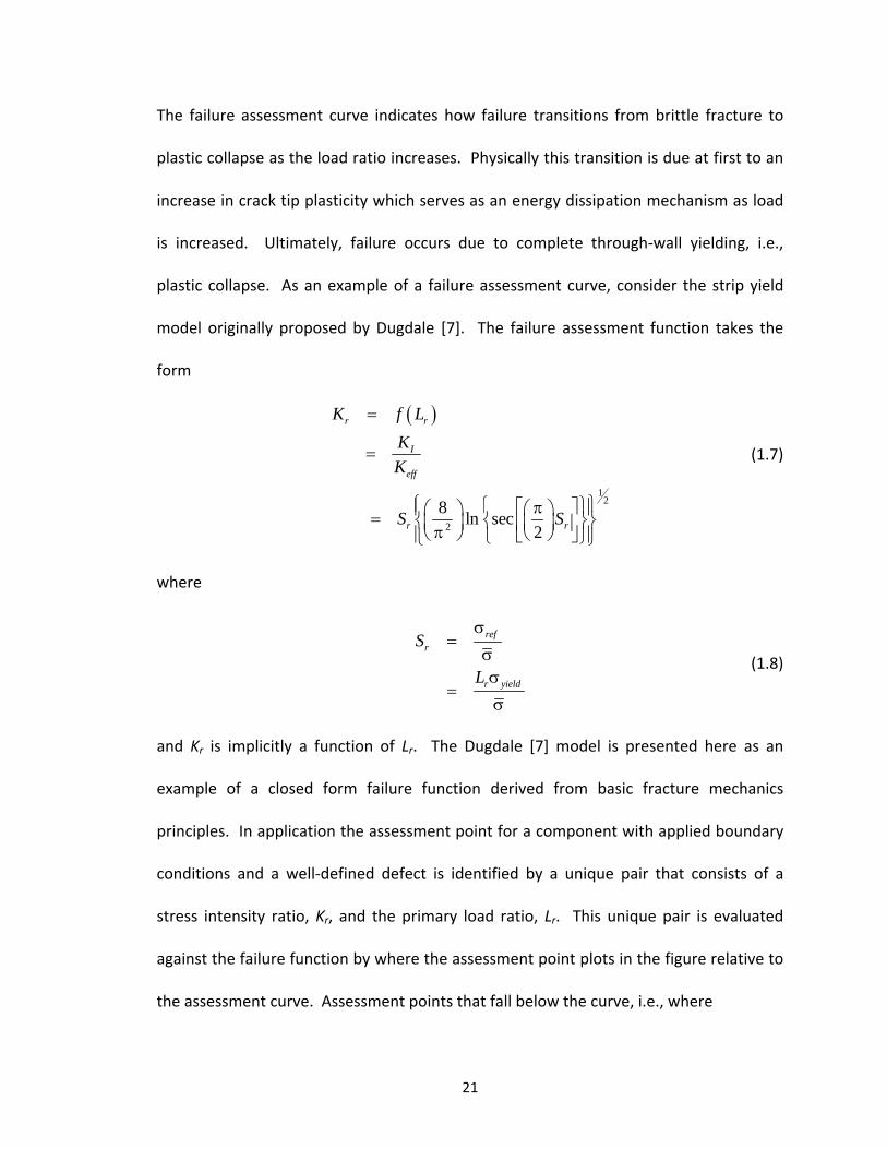
The failure assessment curve indicates how failure transitions from brittle fracture to

plastic collapse as the load ratio increases. Physically this transition is due at first to an

increase in crack tip plasticity which serves as an energy dissipation mechanism as load

is increased. Ultimately, failure occurs due to complete through‐wall yielding, i.e.,

plastic collapse. As an example of a failure assessment curve, consider the strip yield

model originally proposed by Dugdale [7]. The failure assessment function takes the

form

12

2

8ln sec

2

r r

I

eff

r r

K f L

K

K

S S

(1.7)

where

refr

r yield

S

L

(1.8)

and Kr is implicitly a function of Lr. The Dugdale [7] model is presented here as an

example of a closed form failure function derived from basic fracture mechanics

principles. In application the assessment point for a component with applied boundary

conditions and a well‐defined defect is identified by a unique pair that consists of a

stress intensity ratio, Kr, and the primary load ratio, Lr. This unique pair is evaluated

against the failure function by where the assessment point plots in the figure relative to

the assessment curve. Assessment points that fall below the curve, i.e., where

22

,r r r rassessL K K f L

(1.9)

are considered safe and acceptable. Assessment points that fall on or above the curve,

i.e., where

,r r r rassessL K K f L (1.10)

are considered unacceptable and correspond to unstable crack growth or plastic

collapse.

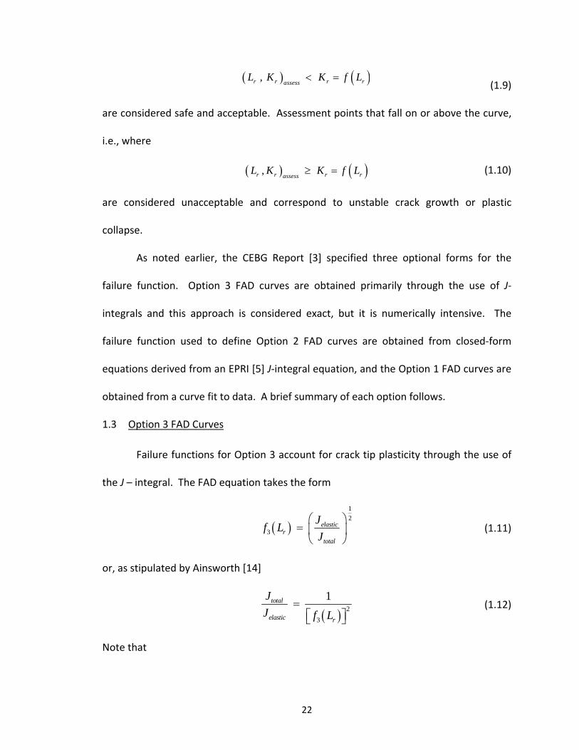
As noted earlier, the CEBG Report [3] specified three optional forms for the

failure function. Option 3 FAD curves are obtained primarily through the use of J‐

integrals and this approach is considered exact, but it is numerically intensive. The

failure function used to define Option 2 FAD curves are obtained from closed‐form

equations derived from an EPRI [5] J‐integral equation, and the Option 1 FAD curves are

obtained from a curve fit to data. A brief summary of each option follows.

1.3 Option 3 FAD Curves

Failure functions for Option 3 account for crack tip plasticity through the use of

the J – integral. The FAD equation takes the form

1

2

3elastic

rtotal

Jf L

J

(1.11)

or, as stipulated by Ainsworth [14]

2

3

1total

elastic r

J

J f L

(1.12)

Note that

23

total elastic plasticJ J J (1.13)

and

2

elastic

KJ

E

(1.14)

where

E E (1.15)

for plane stress and

21

EE

(1.16)

for plane strain. Here is Poisson’s ratio. Although a limited number of closed form

solutions exist, the Jtotal integral used in Option 3 is usually determined through finite

element analysis.


The concepts that support the failure function for Option 2 were derived by

Ainsworth [6] but were based on the Jtotal integral estimation scheme of Kumar and Shih

[8]. Kumar and Shih [8] proposed that in a structural component the Jtotal integral could

be estimated as

12

1'

total elastic plastic

n

eo o

o

J J J

K a Ph b

E P

(1.17)

where

1 1 ,

ah h n

w (1.18)

24

is dimensionless and depends on the crack length, component dimension and the

Ramberg‐Osgood strain hardening exponent (see discussion below). A number of

authors have tabulated values for h1 including He and Hutchison [9] as well as Kumar

and Shih [8]. Note the parameter a represents the actual crack length, and w is the

width of the specimen (w = b + a). Here b is the uncracked ligament length. In the

expression above the material constant E’ = E, is the elastic modulus in plane stress and

E’ = E/(1‐2) in plane strain, where is the Poisson’s ratio. The first term on the right

hand side of Eq. 1.17 corresponds to elastic behavior. The second term of Eq 1.17

represents a fully plastic J‐integral solution in terms of an applied load P, the

characteristic load Po, the yield stress σo, and εo is the strain at the onset of yield. Note

that ae is an effective crack length that Kumar and Shih [8] defined as

2

2

11 1

11

eo

o

n Ka a

n PP

(1.19)

which essentially provides a plastic correction for the elastic term in Eq 1.17. Note that

β = 2 corresponds to plane stress, and β = 6 for plane strain, and K = K(a) in Eq. 1.19.

The Jtotal quantity given by Eq. 1.17 can be evaluated assuming that the Ramberg‐

Osgood stress‐strain relationship applies. The Ramberg‐Osgood relationship was

originally defined as

n

CE E

(1.20)

25

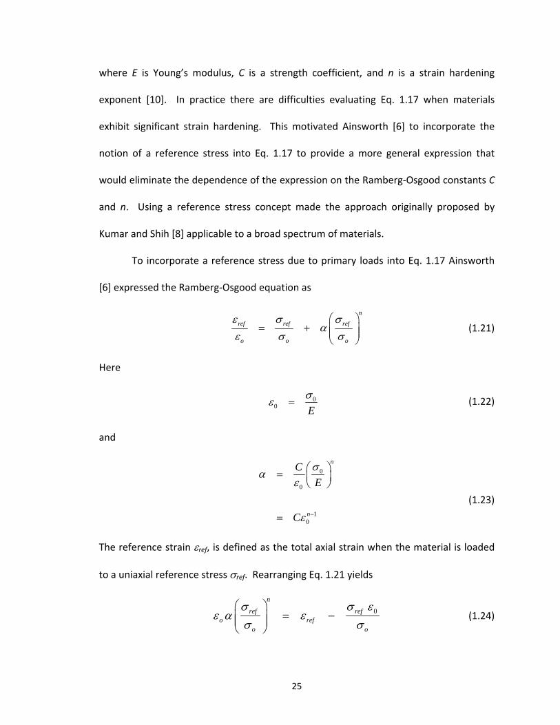
where E is Young’s modulus, C is a strength coefficient, and n is a strain hardening

exponent [10]. In practice there are difficulties evaluating Eq. 1.17 when materials

exhibit significant strain hardening. This motivated Ainsworth [6] to incorporate the

notion of a reference stress into Eq. 1.17 to provide a more general expression that

would eliminate the dependence of the expression on the Ramberg‐Osgood constants C

and n. Using a reference stress concept made the approach originally proposed by

Kumar and Shih [8] applicable to a broad spectrum of materials.

To incorporate a reference stress due to primary loads into Eq. 1.17 Ainsworth

[6] expressed the Ramberg‐Osgood equation as

n

ref ref ref

o o o

(1.21)

Here

00 E

(1.22)

and

0

0

10

n

n

C

E

C

(1.23)

The reference strain ref, is defined as the total axial strain when the material is loaded

to a uniaxial reference stress ref. Rearranging Eq. 1.21 yields

0

n

ref refo ref

o o

(1.24)

26

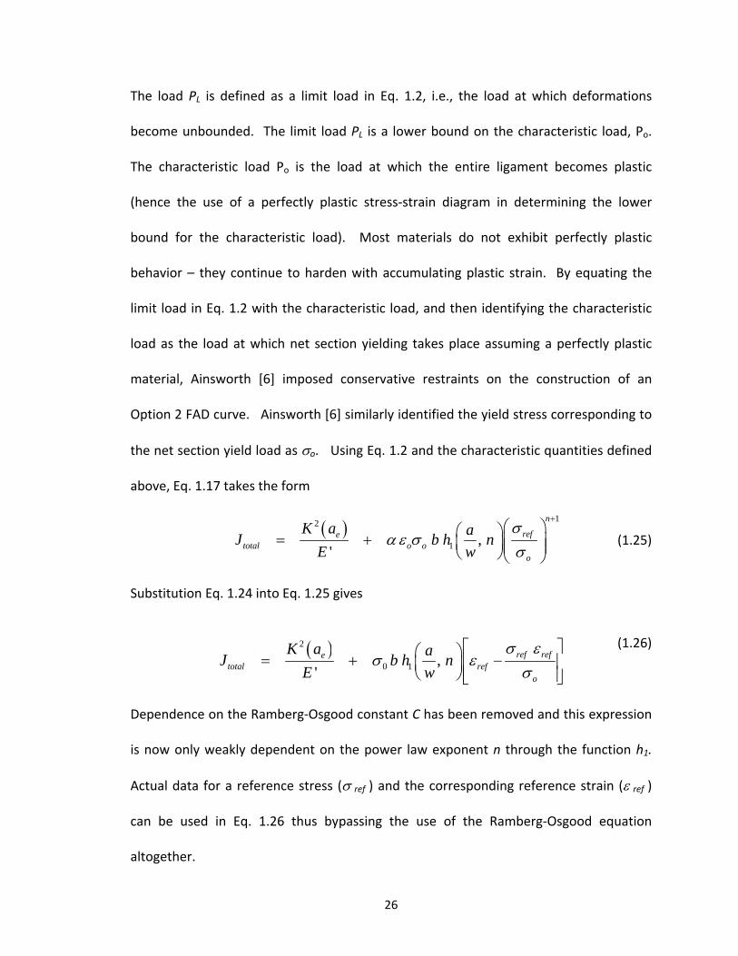
The load PL is defined as a limit load in Eq. 1.2, i.e., the load at which deformations

become unbounded. The limit load PL is a lower bound on the characteristic load, Po.

The characteristic load Po is the load at which the entire ligament becomes plastic

(hence the use of a perfectly plastic stress‐strain diagram in determining the lower

bound for the characteristic load). Most materials do not exhibit perfectly plastic

behavior – they continue to harden with accumulating plastic strain. By equating the

limit load in Eq. 1.2 with the characteristic load, and then identifying the characteristic

load as the load at which net section yielding takes place assuming a perfectly plastic

material, Ainsworth [6] imposed conservative restraints on the construction of an

Option 2 FAD curve. Ainsworth [6] similarly identified the yield stress corresponding to

the net section yield load as o. Using Eq. 1.2 and the characteristic quantities defined

above, Eq. 1.17 takes the form

12

1 ,'

n

refetotal o o

o

K a aJ b h n

E w

(1.25)

Substitution Eq. 1.24 into Eq. 1.25 gives

2

0 1 ,'

ref refetotal ref

o

K a aJ b h n

E w

(1.26)

Dependence on the Ramberg‐Osgood constant C has been removed and this expression

is now only weakly dependent on the power law exponent n through the function h1.

Actual data for a reference stress (ref ) and the corresponding reference strain (ref )

can be used in Eq. 1.26 thus bypassing the use of the Ramberg‐Osgood equation

altogether.

27

The non‐dimensional parameter h1 in Eq. 1.26 is still dependent on the Ramberg‐

Osgood constant n. Ainsworth [6] demonstrated that for special values of the

characteristic load, Po, h1 is independent of n. In addition, Ainsworth [6] recognized that

over a range of n values (n < 20) the ratio of the average value of h1 (i.e., 1h ) to the value

of h1(n = 1) is generally close to unity. When n is taken equal to one

1

1

2

1

,

1

n

refplastic o o

o

refo o

o

aJ b h n

w

b h

(1.27)

where Ainsworth’s [6] notation

1 1, 1 1a

h n hw

(1.28)

has been adopted. Since

0 0E (1.29)

then

2

0 0 10

2

1

1

1

refplastic

ref

J E b hE

E b hE

(1.30)

When n is taken equal to one the fully plastic solution corresponds to the elastic

solution with Poisson’s ratio = 1/2, thus

28

2

2

1 1'

elastic plastic

ref

J J

K aE b h

E E

(1.31)

With

21 (1.32)

and assuming a zero yield offset where

1 (1.33)

then

2 21(1) ( )refb h K a (1.34)

were μ=1 corresponds to plane stress, and μ=0.75 corresponds to plane strain.

Substituting Eq. 1.34 into Eq. 1.26 and assuming a value of Po such that

1 1h h (1.35)

then

2 2

1

1

( ) ( )1

' (1)refe

totalref

EK a K a hJ

E E h

(1.36)

Rearranging yields

22

2

( )( ) '1

' ( )refe

totalref

EK aK a EJ

E K a E

(1.37)

Eq. 1.37 typically underestimates the load carrying capacity of the component by 5% in

the post yield fracture region by assuming the characteristic load is equal to the limit

load, thus using this equation to construct a FAD curve represents a conservative

approximation.

29

To define the Option 2 curve Ainsworth [6] took

12 2

rC

C

KK

K

K a

J E

(1.38)

To define a failure assessment curve Jtotal in Eq. 1.37 is taken equal to the critical value of

the material, i.e.,

22

2

( )( ) '1

' ( )

total C

refe

ref

J J

EK aK a E

E K a E

(1.39)

or

2

2 2

' ( ) '1

( ) ( )refC e

ref

EJ E K a E

K a K a E

(1.40)

From Eq. 1.38

2 2

2

2

'1

( )

( ) '1

( )

C

r

refe

ref

J E

K K a

EK a E

K a E

(1.41)

Note that when Jtotal reaches a critical value JC, the flaw reaches a critical length and the

reference stress as well as the reference strain reach critical values. With

'E

E

(1.42)

and

30

0

r

PL

P (1.43)

then

1

22

21

1ref r

rref r

E LK

L

(1.44)

where, Lr implies load ratios derived from primary loads only ( PrL ). Here ɣ is defined as

2

2 122

2 2

(1) 11 11

1( )

r

e

rr

r

Lbh nK a a

n LL

K aL

(1.45)

Which for small corrections to the crack length simplifies to

1

2 1 1(1)

1

n Kb h

n K a

(1.46)

The choice for is rather arbitrary and the value chosen by Ainsworth [6] was = 1/2

which was obtained from Eq. 1.46 for a through wall crack in an infinite plate in tension

under plane stress conditions in the limit as n approaches infinity. With

1 (1.47)

for plane stress and

1

2

(1.48)

31

for a through wall crack in an infinite plate undergoing far field tensile stresses at the

boundaries, then the Option 2 FAD curve proposed by Ainsworth [6] is obtained from

Eq. 1.44, i.e.,

2

12 2

2

1

2 1

r r

rref

ref r

f L K

LE

L

(1.49)

The material properties needed to plot this FAD curve are Young’s modulus (E), the yield

stress (yield), the ultimate stress (ult) , as well as stress and strain information that can

be obtained directly from experimental data.


Ainsworth [4] pointed out that the Option 1 failure function is a curve fit

obtained from an amalgamation of material properties biased towards the lower bound

of material specific curves generated using the Option 2 FAD curves. The lower bound

estimate is valid for LrP < 1, σyield > 40 ksi, and for materials with hardening exponents

greater than ten (n > 10), as shown in Figure 1.2. The functional form of the Option 1

FAD curve is

2 61( ) (1 0.14 )[0.3 0.7 exp( 0.65 )]r r rf L L L (1.50)

This function has been modified slightly from its original formulation to better match

the Option 2 curves at intermediate values of Lr [11]. This modified curve was originally

presented in Harrison et al. [12] where the revised Option 1 FAD curve is expressed as

2 1/2 61 mod( ) (1 0.5 ) [0.3 0.7 exp( 0.6 )]r r rf L L L (1.51)

32

Through the years these expressions have been developed and refined through a

consensus process by various Code committees.

Figure 1. 2: Option 1 and Option 2 FAD Curves based on the Ramberg‐Osgood Material Model

(σyield = 38.4 ksi, σult = 74.1 ksi, E= 25850 ksi, a = 1, εo = 0.002)

Option 2 and Option 3 curves are material dependent, i.e., they are both

functions of the material stress‐strain curve. However, Option 1 is a lower bound curve

fit to a group of Option 2 curves that were based on materials characterized by

Ramberg‐Osgood stress‐strain relations and all materials within the group have the

same yield stress (~40 ksi). Therefore the Option 1 FAD curve may not represent a

lower bound for materials with yield stresses below 40 ksi. As a result, the Option 1

curve has limited applicability when stress‐strain relationships are not approximated

well by the Ramberg‐Osgood model and when the yield stress of the material is less

than 40 ksi. This is evident in Figure 1.3 where an Option 1 curve is compared to an

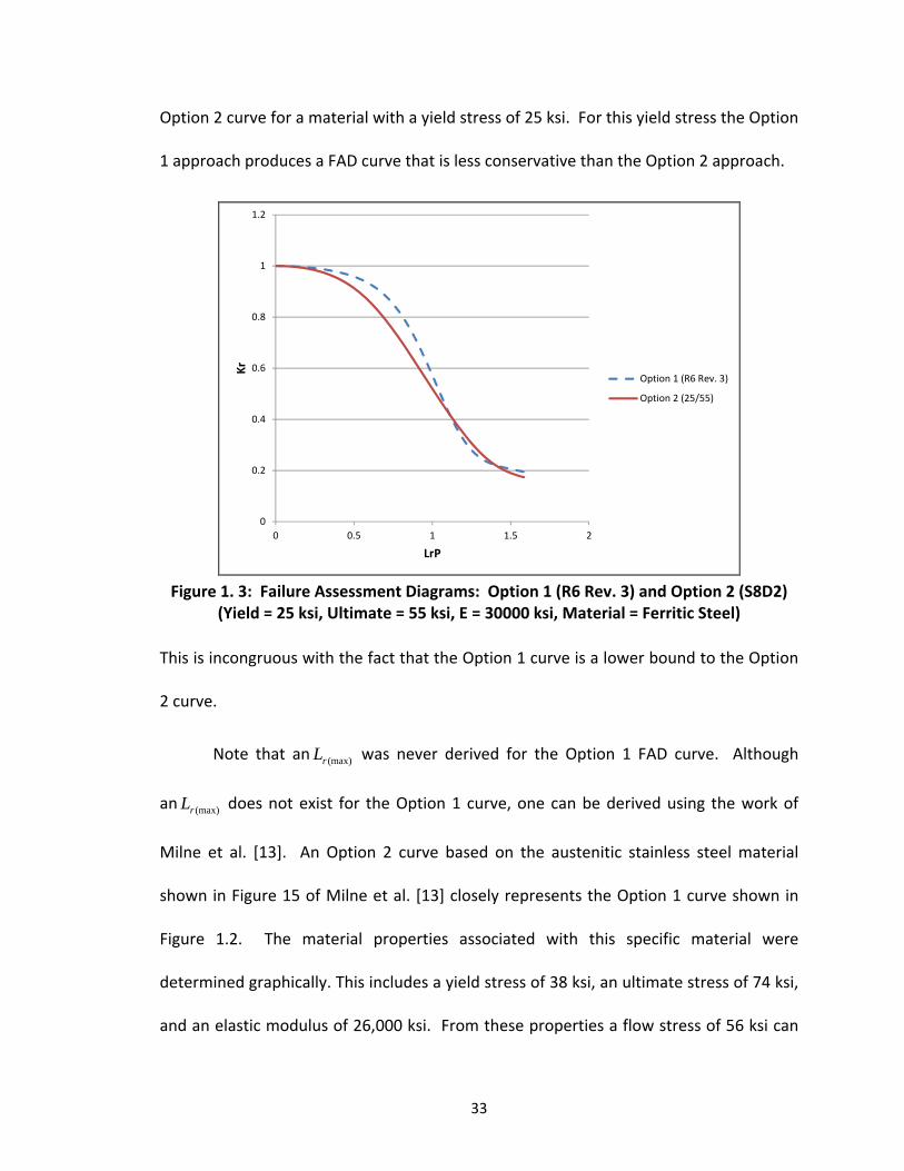
33

Option 2 curve for a material with a yield stress of 25 ksi. For this yield stress the Option

1 approach produces a FAD curve that is less conservative than the Option 2 approach.

0

0.2

0.4

0.6

0.8

1

1.2

0 0.5 1 1.5 2

Kr

LrP

Option 1 (R6 Rev. 3)

Option 2 (25/55)

Figure 1. 3: Failure Assessment Diagrams: Option 1 (R6 Rev. 3) and Option 2 (S8D2) (Yield = 25 ksi, Ultimate = 55 ksi, E = 30000 ksi, Material = Ferritic Steel)

This is incongruous with the fact that the Option 1 curve is a lower bound to the Option

2 curve.

Note that an (max)rL was never derived for the Option 1 FAD curve. Although

an (max)rL does not exist for the Option 1 curve, one can be derived using the work of

Milne et al. [13]. An Option 2 curve based on the austenitic stainless steel material

shown in Figure 15 of Milne et al. [13] closely represents the Option 1 curve shown in

Figure 1.2. The material properties associated with this specific material were

determined graphically. This includes a yield stress of 38 ksi, an ultimate stress of 74 ksi,

and an elastic modulus of 26,000 ksi. From these properties a flow stress of 56 ksi can

34

be computed using Eq. 1.5 and an (max)rL of 1.46 can be computed using Eq. 1.4. Hence,

by using the austenitic steel from Milne et al. [13] to represent the Option 1 FAD curve

behavior, Ainsworth was able to validate the Option 1 FAD curve and determine its

limiting properties.

1.6 Effects from Load Combinations

The assessment curves are also dependent on whether stresses in the

component being assessed are generated from primary or secondary loads. If thermal

or residual stresses (secondary loads) are present prior to the primary loads being

applied, an adjusted failure assessment curve could take secondary loads into account.

However Ainsworth [14] developed a simpler approach. The failure curve that

combines mechanical (primary) and thermal loads (secondary) will lie both above and

below the FAD curve for primary loads only. This is shown in Figure 1.4. The dashed

line depicts the effects the combined load has on calculating Jelastic and Jtotal, i.e., the

dashed line represents the more exact Option 3 curve. Assuming a material is linear

elastic, then by superposition Jelastic simply adds the primary and secondary load effects.

However, Jtotal includes nonlinear effects such as material hardening, and the primary

load effects cannot be simply added to the secondary load effects.

Thermal stresses and residual stresses from welding are examples of secondary

stresses. FAD curves are developed assuming proportional loads are applied to the

component being assessed. Components subject to secondary stresses prior to primary

stresses being applied are subject to non‐proportional loads. The effect of non‐

proportional loading is a change in the shape of the FAD. This change in shape is

35

0

0.2

0.4

0.6

0.8

1

1.2

0 0.2 0.4 0.6 0.8 1 1.2 1.4 1.6

Kr

LrP

Mechanical Only

Mechanical + Thermal

Figure 1. 4: The Effects of Thermal Stress on the Mechanical Stress FAD Curve

(Option 2 FAD Curve: σyield = 40.0 ksi, σult = 70.0 ksi, E = 25850 ksi, LrS = 1.25)

dependent on the specific amount and type of secondary stress applied as suggested in

Figure 1.4.

Since secondary stresses contribute to the driving force of the crack at low to

moderate primary stress levels, Jtotal is influenced by an increase in crack tip plasticity

that causes a decrease in the stress intensity ratio as primary load is applied to the

component under analysis. As the primary load increases this effect diminishes. The

FAD curve will increase beyond the level of the “primary stress only” FAD curve due to

the inclusion of both primary and secondary stresses in the Jelastic solution.

The inclusion of secondary stresses in a FAD analysis requires the calculation of a

specific FAD curve for a particular primary and secondary load combination. Creating a

specific FAD for each combined load case is cumbersome. Typically this requires a finite

element analysis with a pre‐determined residual stress field, thus alternative solutions

36

have been developed. Alternative solutions range in complexity due to the types of

application, for example: Turner [15] applies a fractional power addition of the

mechanical and residual J values; Chell [16] suggests a graphical approach which

involves moving the origin of the FAD based on the amount of secondary stress and

evaluates the primary stress using the resulting shifted FAD; and Ainsworth [14] applies

a load combination factor, , to the stress intensity ratio coordinate of the assessment

point to account for the difference between the “primary stress only” and the combined

stress FAD curves. Current revisions of the published standards that incorporate FAD

assessments such as API‐579‐1/ASME FFS‐1 [1] and CEGB report R/H/R6 [3] use load

combination factors based on Ainsworth’s development [14]. By doing this only one

assessment curve is needed regardless of the type of loads applied. The factor is a

function of both primary and secondary loads. Unfortunately, Ainsworth only

developed this approach for the Option 1 curve. The work presented here expands on

Ainsworth’s [14] efforts by using his methodology to develop load combination factors

for Option 2 curves based on ASME B&PV Code Section VIII, Division 2 [17] material

properties, and the Prager [18] stress‐strain relationship.

1.7 Scope and Objectives

The scope of this thesis includes developing load combination factors for Option

2 FAD curves and tabulating these factors for a variety of yield and ultimate stress

values. In essence this work will admit the effects of secondary stresses (thermal/weld

residual stresses) on the Option 2 FAD failure functions based on material stress‐strain

relations defined in ASME B&PV Code Section VIII, Division 2 [17]. The objective of this

37

thesis is three‐fold. First the level of conservatism is evaluated in the use of the Option

1 FAD failure functions relative to Option 2 curves. The relative conservatism of the

Option 1 approach to the Option 2 approach was briefly discussed earlier in reference to

Figure 1.3. In addition, the sensitivity of the factors to known errors in the material

properties used to generate the factors will be assessed. Finally, recommendations are

provided for Code updates that incorporate the use of the material specific factors.

38

CHAPTER II ‐ AINSWORTH’S APPROACH

2.1 Thermal and Residual Stresses

The influence that secondary (thermal) stress has on the crack tip stress state is

illustrated in Figure 2.1. Both curves depicted represent a ratio of Jtotal to Jelastic as a

function of the load ratio,PrL . The dashed curve in Figure 2.1 represents an increasing

primary (mechanical) load applied subsequent to an existing fixed secondary (thermal)

load. The solid curve is a result of only an increasing primary load. Since the secondary

stress is present prior to the application of primary loads (non‐proportional loading), the

J‐integral ratio for combined primary and secondary stresses (dashed line) has an initial

value greater than that of a component subject to primary loads alone (solid line). As

the primary load increases the difference between the two curves widen due to the

increased plastic zone near the crack tip as a result of the secondary stress. At some

point the rate of change in the primary stress curve overtakes the rate of change in the

combined stress curve. As primary loading continues both curves begin to take on the

same rate of change. The magnitude of this effect is proportional to the amount of

39

secondary stress applied. This effect will be referred to in this work as the “secondary

stress effect.”

0

2

4

6

8

10

12

14

16

18

0 0.2 0.4 0.6 0.8 1 1.2 1.4 1.6

J tot/J el

LrP

Mechanical Only

Mechanical + Thermal

Figure 2. 1: Schematic Showing the Effects of Thermal Residual Stresses

on J Integral Calculations

When conducting a failure assessment for a component, it is necessary to

include the effect that the secondary stress has on the stress intensity factor. In the

elastic stress regime the effects are easily accommodated. Here the stress intensity

from the secondary stress is simply added to the stress intensity from the primary load

invoking the superposition principle for linear functions. In the inelastic stress regime

the cumulative effects of secondary stresses along with stress from the primary loads do

not combine in a straightforward manner due to nonlinearities. To account for this one

can include secondary stresses and determine J‐integral values from a combination of

primary and secondary loads using finite element analyses. Ainsworth [14] proposed a

simpler approach that bypasses the need for a finite element analysis by adding a load

40

combination factor to the sum of the primary and secondary elastic stress intensity

ratios. This method corrects for any effects that secondary stresses have on the FAD

curve. Ainsworth’s [14] approach to account for the effect of secondary stresses is

explored in this Chapter.

2.2 Ainsworth’s Reference Stress Concept

In the discussion on FAD curves in the previous chapter

2

1

( )total

Pelastic r

J

J f L (2.1)

and

PrefP

ryield

L

(2.2)

were defined. Here the superscript “P” denotes the load ratio and the reference stress

are the result of primary (mechanical) loads on a component. Thus

2

1totalP

elastic ref

yield

J

Jf

(2.3)

Keep in mind that using the reference stress removes component geometry dependence

from the functional form of the FAD curve. Without loss of generality the elastic stress

intensity factor can be expressed as

1

2P PI refK a (2.4)

for mode I fracture. With

41

2

1p

elastic

KJ

E (2.5)

Solving Eq. 2.1 for Jtotal yields

2

Pref

total Pref

yield

aJ

Ef

(2.6)

In the context of this work thermal and residual stresses behave as local stresses and do

not tend to lead to plastic collapse; therefore, the plastic term in Eq. 1.17 for Jtotal can be

neglected. When estimating Jtotal for secondary stresses Ainsworth [14] assumes that

2S

J

total elastic

KJ J

E (2.7)

Here KJS is the elastic stress intensity factor for the secondary stress corrected for crack

tip plasticity. Setting Eq 2.7 equal to Eq. 2.6 yields

S Sref J

Sref

yield

K

af

(2.8)

Note that the quantity on the left side of Eq. 2.8 represents an effective reference stress

one that is adjusted for crack tip plasticity through the use of the FAD function.

Ainsworth [14] used the Option 1 FAD curve equation with the secondary reference

stress defined as

S Sref r yieldL (2.9)

Thus

42

2 6

1( ) 1 0.14 0.3 0.7 exp 0.65S Sref refS

ryield yield

f L

(2.10)

The secondary stress effect is inherently a plasticity phenomenon and if the material is

linear elastic (LEFM), the secondary stress effect will not occur and superposition can be

invoked and the primary and secondary stress intensity ratios are added together to

obtain a composite value for use in the FAD. However, when either the primary or

secondary stress states are the result of nonlinear behavior, i.e., crack tip plasticity, a

more in depth treatment is needed.

The next step is estimating what Ainsworth [14] proposed as an equivalent

mechanical stress that represents the combined stress state. This single mechanical

stress quantity generates an equivalent J‐integral for the actual component being

assessed. He derived this combined quantity, i.e., σCref, by comparing the displacement

of a component, where the actual primary and secondary stresses are applied, to the

displacement of the component where secondary (thermal) stress is replaced with an

additional constant mechanical load. Ainsworth [14] made the comparison through the

application of energy principles. The actual component assessed has an initial

secondary (thermal) stress distribution and a primary (mechanical) stress is

subsequently imposed (non‐proportional loading). The application of the primary load

is represented by a time‐like variable t, as P(t). The deformation from this analysis is

compared to the deformation of the component with the same geometry but now the

actual secondary stress is replaced by an additional primary stress from a constant load

43

identified as R. Using work – energy principles the displacements in both components

are related through the expression

0

T

VR u u p p dVdt (2.11)

The expression above is formulated on a uniaxial basis and represents the difference in

stored internal energy. On the left hand side Δu* is the increase in displacement under

the load R between time t = 0 and t = T. On the right hand side of the equation σ is

stress, is the elastic strain rate, p is the plastic strain rate, V is the volume, and t

represents a time‐like variable. Starred quantities on the right hand side are those in

the component where the constant load R is applied. Unstarred quantities are those

associated with the actual structure.

Ainsworth [6, 19] uses an interpretation of a deformation bounding theorem

from plasticity to estimate the equivalent mechanical load. Use of this theorem enables

the computation of an upper bound on the deformation of an equivalent component

with no thermal load but an increased mechanical load. The following upper bound can

be established from Eq. 2.11

0 0R u R u A A T R u A (2.12)

If the material hardens linearly then

1

2VA p p dV (2.13)

Note that is the elastic stain energy density function which is dependent on both

stress and strain, i.e.,

44

1,

2 (2.14)

and is a kinematic hardening parameter since bounding theorems assume perfect

plasticity. It is assumed that the displacements of interest for estimating the J‐integral

can be related on average to the values of strain at a reference stress. In general A(T)

will be unknown but since A is positive a conservative estimate of the upper bound

omits A(T) [6, 19]. In the actual component the reference stress is σSref at t = 0 and σCref

at t = T. In the component with the dummy load, the reference stress is σRref at t = 0,

and (σRref + σPref) at t = T. At time t = 0 Eq. 2.14 has the following estimated value for

elastic strain energy

2

,2

R Sref ref

E

(2.15)

and the following estimated value for plastic strain energy

1 1

2 2

R Sref refR S R S

ref ref ref refp pE E

(2.16)

Ainsworth [14] points out that is the uniaxial strain for a given value of stress, .

Therefore the total strain energy for Eq. 2.13 becomes

10

2R S R Sref ref ref refA V (2.17)

Similarly applying the work energy principles in order to estimate Δu and Δu* result in

R P R Rref ref ref refR u V (2.18)

and

45

R C Sref ref refR u V (2.19)

With this upper bound on the deformation one can then compute an estimate of the

equivalent reference stress. In his development Ainsworth [14] assumed that the

mechanical and thermal loads act to reinforce each other, i.e., both contribute to an

increase the equivalent stress intensity value. The equivalent mechanical reference

strain can be calculated by substituting Eq. 2.17, Eq. 2.18 and Eq. 2.19 into Eq. 2.12

which leads to

[ ][ ( ) ( )]( ) ( )

2

S R S Rref ref ref refC P R

ref ref ref Rref

(2.20)

Here the dummy reference stress is defined as

PrefR

ref

R

P

(2.21)

A value for R is selected such that ε(σCref) in Eq. 2.20 is minimized. This produces an

optimum or least upper bound on deformation.

Since Ainsworth [14] reasoned that the approach developed above for primary

and secondary stresses results in an equivalent applied mechanical strain then one can

estimate the combined equivalent reference stress, σCref, from

2

Cref

total Cref

yield

aJ

Ef

(2.22)

where the superscript “C” denotes combined. In addition, an equivalent mechanical

load, PC, can be obtained from the expression

46

C C Lref

yield

PP

(2.23)

Estimating the equivalent reference stress σCref for the combined loads first requires

knowledge of the primary reference stress σPref and the reference stress for the

secondary load alone, σSref.

The general formulation for an Option 2 FAD curve was expressed in Eq. 1.49.

Also recall that an Option 1 FAD curve was derived as a lower bound to the Option 2

FAD curves. So Ainsworth [14] also treated Eq. 1.49 as a general expression for the

Option 1 FAD curve. This equation was comprised of two terms. The first term

describes both elastic and fully plastic behavior. The second term represents minor

corrections when bulk behavior of the component is elastic but the J‐integral exceeds

the elastic value. Essentially, Ainsworth [14] argued that Eq 1.49 can be used in general

to characterize an Option 1 FAD curve if the second term is ignored. Ignoring the

second term and solving Eq. 1.49 for ( )ref leads to

21

( )/ref

ref

ref yieldf E

(2.24)

This is essentially a linear stress‐strain relationship with the Option 1 FAD equation

embedded in the expression. This relationship can be substituted for every occurrence

of strain in Eq. 2.20 and the result is Eq. 2.25. This expression allows the computation of

Cref for a set of primary and secondary reference stresses along with an optimized

Rref value.

47

21

21

2 21 1

1

( / )

( )1

(( ) / )

[ ]

2 ( / ) ( / )

CrefC

ref Cref yield

P Rref ref

P Rref ref yield

S R S Rref ref ref ref

R S Rref ref yield ref yield

E f

E f

f f

(2.25)

2.3 Ainsworth’s Secondary Stress Correction Factor

Ainsworth developed a correction factor identified here as , which is added to

the sum of the primary and the secondary stress intensity ratios in the following manner

P Sr r rK K K (2.26)

Here KrP is the stress intensity ratio associated with the primary mechanical loads, and

KrS is the stress intensity ratio associated with secondary thermal stresses and/or

residual stresses. This approach allows Kr to be adjusted for the effects of secondary

stress without changing the definition of Lr, thereby conforming to the methodology of

Harrison et al. [3].

To determine Ainsworth proposed that both

1

PS PrefI I

Ic Ic yield

K Kf

K K

(2.27)

and

1/2

1

( )C Cref ref

Ic yield

af

K

(2.28)

define a failure assessment curve. Rearranging Eq. 2.27 yields

1

P P Sref I I

yield Ic Ic

K Kf

K K

(2.29)

48

The expression

1/2

1

( )Cref

Ic Cref

yield

aK

f

(2.30)

can be obtained from Eq. 2.28. Substituting Eq. 2.30 into Eq. 2.29 for KIc yields

1 1 1/2 1/2( ) ( )

P C P Sref ref I I

C Cyield yield ref ref

K Kf f

a a

(2.31)

Substituting KIP from Eq. 2.4 and KI

S from Eq. 2.8 into this last expression yields

1 1

1

1

( / )

P C Sref ref refP

refC Syield yield ref ref yield

f ff

(2.32)

The ψ factors from Ainsworth’s original work [14] are recreated and shown in Figure 2.2.

These curves are functions of both primary and secondary load ratios through the stress

quantities employed. The maximum secondary load ratio, SrL , defined in Ainsworth’s

results is 1.1.

Note that Ainsworth [14] as well as Hooten and Budden [20] point out when the

primary load is zero the equivalent combined stress, σCref, is equal to the secondary

stress, σSref, as it should. Similarly, as the secondary stress, σSref, decreases, the

equivalent combined stress, σCref, approaches the primary mechanical stress, σPref.

49

Figure 2. 2: Variation of the ψ1 Factor with Mechanical and Thermal Loads [14]

Ainsworth [14] also included a plot of the maximum ψ factor as a function of

/ ( )S Sr rL f L and that plot is reproduced here in Figure 2.3. The horizontal axis in this

figure is based on the relationship found in Eq. 2.6 but as a function of σSref, instead of

σPref . With

2

1

SrefS

total Sref yield

aJ

Ef

(2.33)

once the assumption is made that

2

S Stotal elastic

SJ

J J

K

E

(2.34)

for small values of Sref. Substitution of Eq. 2.34 into Eq. 2.33 leads to

50

22

/

S SJ ref

Sref yield

K a

E Ef

(2.35)

Simplification yields

1/2

/

S Sref J

Syieldyield ref yield

K

af

(2.36)

Finally, recognizing that

/S S

ref yield rL (2.37)

results in

1/2

SSJr

Sr yield

KL

f L a (2.38)

the units Ainsworth [14] used for this figure in his original work.

0.000

0.050

0.100

0.150

0.200

0.250

0 1 2 3 4 5 6

Max ψ1

LrS/f(Lr

S)

Figure 2. 3: Values of the Maximum Shift of ψ1 Curve, [14]

51

In summary, a key feature of Ainsworth’s [14] development is the assumption

that for secondary stresses due to thermal/residual plasticity corrections can be

neglected. This assumption allows Ainsworth to replace totalJ with elasticJ in Eq. 2.7 and

Eq. 2.34. As later noted by Hooton and Budden [20] this assumption leads to non‐

conservative results for intermediate values of Sref , where S S

J IK K ; and overly

conservative results for high values of Sref , where S S

J IK K . Here SJK is a stress

intensity factor for secondary stresses corrected for plasticity. A graphical

representation of this is depicted in Figure 2.4 in terms of JStotal and JSelastic. Note the

assumption used by Ainsworth [14] is identified as JSelastic*. JSelastic* is Ainsworth’s

approximation for JStotal. Hooton’s and Budden’s [20] assessment of Ainsworth’s

assumption is corroborated by the results depicted in Figure 2.4. JSelastic*

underestimates JStotal for intermediate values of Sref and overestimates JStotal for high

values of Sref .

To address this issue, Hooton and Budden [20], developed a correction factor

that corrects the ψ factor for these situations. The adjusted ψ factor is

1

SI

adjusted SJ

K

K

(2.39)

where

/

/

C Sref yield ref

C Sref ref yield

f

f

(2.40)

52

Figure 2. 4: Ainsworth’s Secondary Stress Assumption

The Hooton and Budden [20] approach adjusts ψ based on the level of secondary

stress applied. At low levels of secondary stress their approach returns the values

determined by Ainsworth [14]. The key to their approach is determining the value

of SJK , the inelastic stress intensity factor for the secondary stress. This value is used

along with the elastic stress intensity factor for the secondary load to adjust the

factor.

2.4 Published ψ Factors

Ainsworth [14] published ψ1 factors in a graphical format. His Figure 4 depicts

variations with mechanical load and his Figure 5 depicts variations with respect to

thermal/residual stresses. Results from Ainsworth’s [14] Figure 4 are recreated here in

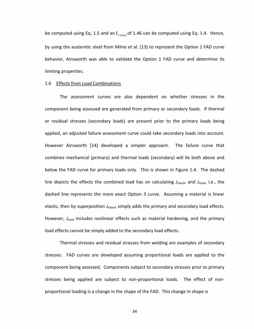
Figure 2.5 to demonstrate an ability to compute ψ1 factors properly. Since Ainsworth

did not publish tabulated data for ψ1 factors, a comparison of the factors presented in

53

Figure 2.5 and Ainsworth’s [14] original computations must be conducted visually. The

curves in Figure 2.5 appear to be a faithful reproduction of the original work by

Ainsworth [14].

Figure 2. 5: Recalculated ψ1 Values Based on the Option 1 FAD Curve

Ainsworth’s [14] Figure 5 depicts maximum ψ1 as a function

of 1 2SJ yieldK a . This graph is reproduced in Figure 2.6 to further validate that

calculated quantities from this effort are being computed properly. Note that the

maximum ψ1 factors in Figure 2.6 are plotted as a function of Sr

Sr LfL and not as a

function of 1 2SJ yieldK a . These two quantities were equated earlier in Eq. 2.38.

Maximum ψ1 values from Ainsworth’s [14] Figure 5 were determined by inspection. The

comparison in Figure 2.6 confirms that the maximum ψ1 factors computed here are

consonant with Ainsworth’s [14] original results.

54

Harrison et al. [3] present tabulated ψ1 factors but it is not clear how these

values were generated. However, visual comparisons between the tabulated values and

calculated values from this effort indicates that both match. Two graphical comparisons

are presented in Figures 2.7 and Figure 2.8 for the case of 481.0SrL and 28.1S

rL ,

respectively. Data for all intermediate value of SrL match in a similar fashion.

Figure 2. 6: Comparison Between Calculated and Tabulated Max ψ1Values

(yield = 38.4 ksi, ult = 74.1 ksi, E = 25850 ksi)

In their Table A4.1 Harrison et al. [3] publishes values of ψ1 factors as a function

of the primary load ratio, PrL , running down the table from zero to two in increments of

0.1. In addition, the table values of ψ1 factors are functions of secondary load which

Harrison et al. [3] quantified using the ratio S P PJ I rK K L . In the referenced Table A4.1

this ratio runs across the table from zero to five in increments of 0.5. This measure of

secondary load can be interpreted in terms of the ratio /S Sr rL f L through the use of

55

Figure 2. 7: Values of ψ1 for Lr

S = 0.481


Figure 2. 8: Values of ψ1 for Lr

S = 1.28


56

relationships derived earlier in the thesis. Substituting Eq. 2.2 for PrL and Eq. 2.4 for P

IK

in the ratio used by Harrison et al. [3] becomes

1 2

1 2

S SJ J

P P PI r ref

Pref

yield

SJ

yield

K K

K L a

K

a

(2.41)

Earlier it was noted that the right hand side of Eq. 2.41 was equal to Sr

Sr LfL by way of

Eq. 2.38, thus

/

S SJ r

P P SI r r

K L

K L f L (2.42)

The tabulated values provide by Harrison et al. [3] appear again in Tables 9.4 of API‐579

[1], however API‐579 [1] publishes ψ1 factors in terms of values for PrL and

SRrL . The

load ratio SRrL is defined in API‐579 [1] as the ratio of yield

SRref and the definition of

SRref is identical to the definition of S

ref used in this thesis. Thus load ratio SRrL from

API‐579 [1] is identical to the load ratio SrL used in this thesis and

S SSRJ rrP P S

I r r

K LL

K L f L (2.43)

The ψ1 factors published in API‐579 [1] are correct values – one need only compare

Table A4.1 from Harrison et al. [3] with Table 9.4 in API‐579 [1] to verify that. However,

the values of SRrL used in API‐579 [1] are not consonant with the values of S P P

J I rK K L

used in Harrison et al. [3]. Table 2.1 provides equivalent values of SrL with the values of

57

S P PJ I rK K L = 1/S S

r rL f L used by Harrison et al. [3]. This misinterpretation also

occurs in the published data of the φ1 factors in Tables 9.6 of API‐579 [1] and can be

corrected using Table 2.1. Values of ψ1 and φ1 based on the current published incorrect

values of SRrL for S P P

J I rK K L = 1/S Sr rL f L would be non‐conservative, i.e., values of

ψ1 would be underestimated. However, for SrL < 0.5, SR

rL and 1/S Sr rL f L are essentially

equivalent so errors would be negligible.

Table 2. 1: ψ1 Factor Secondary Stress Load Ratio Conversion Table

S P PJ I rK K L =

1/S Sr rL f L

SRrL

0 0.0

0.5 0.481

1.0 0.801

1.5 0.972

2.0 1.045

2.5 1.099

3.0 1.149

3.5 1.169

4.0 1.226

4.5 1.276

5.0 1.285

58

CHAPTER III ‐ STRESS‐STRAIN MODELS

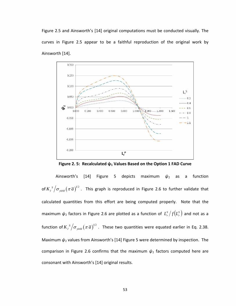
3.1 Ramberg‐Osgood Model

In Chapter 1 the Option 2 FAD curves are functionally dependent on specific

values taken from a material’s stress‐strain diagram, as indicated by Eq. 1.49. These

values could be obtained directly from experimental data if this data were available.

Typically, the stress‐strain values are obtained from the curves in ASME Boiler &

Pressure Vessel Code Section VIII, Division 2, Annex 3D. There are two approaches to

mathematically modeling stress‐strain curves, the Ramberg‐Osgood equation and the

Prager approach.

Much of the early developments in elastic‐plastic fracture mechanics used a

power law known as the Ramberg‐Osgood relationship to fit material’s stress‐strain

data. The Ramberg‐Osgood relationship is expressed as

n

CE E

(3.1)

where E is Young’s modulus, C is a strength coefficient, and n is a strain hardening

exponent [10]. If one plots true stress versus true strain on a log‐log plot the slope of

this curve should yield the hardening exponent, n. However, many materials have flow

59

behavior that does not plot as a straight line on a log‐log plot. This makes the use of the

Ramberg‐Osgood equation problematic. Low carbon steels, for instance, exhibit a strain

hardening exponent that is different near the proportional limit in comparison to large

strains. In these situations using the Ramberg‐Osgood expression to represent this type

of behavior can lead to significant errors in deriving fracture assessment curves [9].

A function that captures bi‐linear and non‐linear stress‐strain responses was

developed by Prager [18]. This stress‐strain model has been approved as an option for

use in Section VIII, Division 2 of the ASME B&PV Code [17]. Prager’s development of the

stress‐strain relation utilizes two hardening exponents ( 1m and 2m ) and captures the

bilinear behavior mentioned above. In Prager’s model [18] there are two nonlinear

terms identified here as 1 and 2 . Each non‐linear term is associated with the

previously identified hardening exponents. The nonlinear terms each contain a

hyperbolic tangent function and as a result of combining the two hyperbolic terms

additively a smooth transition is attained between the regions each term serves to

model.

3.2 Prager Model

The Prager [18] stress‐strain relation has been incorporated into Section VIII,

Division 2, of the ASME B&PV Code, for use with materials found in Section II, Part D of

the ASME B&PV Code. The complete description of the model is as follows

1 2t

t s E

(3.2)

where, t is the true stress, t s is the true strain corresponding to t , and

60

11 1.0 tanh

2H

(3.3)

22 1.0 tanh

2H

(3.4)

For 1

1

1

11

mt

A

(3.5)

11

1

ln 1

yield ys

m

ys

A

(3.6)

and

1

ln

ln 1ln

ln 1

p ys

p

ys

Rm

(3.7)

where the parameters in the expressions have been identified above. Note that

0.002ys (3.8)

is utilized by this model and represents the 0.2% offset strain. For 2

2

1

22

mt

A

(3.9)

and

2

22

2

expultimatem

mA

m

(3.10)

As noted in the table below the parameters 2m is a function of the stress ratio R, where

yield

ultimate

R

(3.11)

61

Table 3. 1: Stress‐Strain Curve Parameters [18]

Material Temperature Limit 2m p

Ferritic Steel 480C (900F) 0.60 1.00 R 2.0E‐5

Stainless Steel and

Nickel Base Alloys 480C (900F) 0.75 1.00 R 2.0E‐5

Duplex Stainless

Steel 480C (900F) 0.70 0.95 R 2.0E‐5

Precipitation

Hardened Nickel

Base

540C (1000F) 1.90 0.93 R 2.0E‐5

Aluminum 120C (250F) 0.52 0.98 R 5.0E‐6

Copper 65C (150F) 0.50 1.00 R 5.0E‐6

Titanium and

Zirconium 260C (500F) 0.50 0.98 R 2.0E‐5

For both 1 and 2 the parameter H used in the hyperbolic functions

2 t yield ultimate yield

uttimate yield

KH

K

(3.11)

The parameter K in the equation above is defined as

1.5 2.5 3.51.5 0.5K R R R (3.13)

The required inputs to calculate the true strain using equation 3.2 are the

nominal yield stress, yield , the ultimate engineering stress, ultimate , elastic modulus, E,

and the plastic strain associated with the nominal proportional limit, ys . Values for

yield , ultimate , E, and ys are estimated by inspection from the stress strain curve of a

particular material. Relationships for the parameters 2m and values of

p for various

62

materials can be found in Prager [18]. These parameters along with their

corresponding temperature limits are provided in Table 3.1.

Recall that the Option 1 FAD curve is a single curve that represents an

amalgamation of properties in order to produce a conservative lower bound for failure

assessments. The stress‐strain curves associated with the Option 1 FAD curve is shown

in Figure 3.1. For comparative purposes the true‐stress true‐strain curves from both the

Ramberg‐Osgood and the Prager models for the Option 2 curve are depicted as well. In

this figure the Ramberg‐Osgood (R.O.) model is depicted for two hardening exponents, n

= 6 and n = 7. The Prager model is shown for three yield‐to‐ultimate stress ratios, R =

30/50, R = 30/70, and R = 30/90. This Option 1 FAD curve is used to calculate the

equivalent mechanical reference stress discussed in Chapter II (see Eq. 2.24). All curves

shown in Figure 3.1 are depicted using a yield stress of 30 ksi, and an elastic modulus of

30,000 ksi.

Note that from Eq. 1.50 the Option 1 FAD function equals zero for Lr = 2.67, and

this is shown graphically in Figure 3.2. As a result when the scale for the true strain is

greatly extended in Figure 3.1 the true stress‐strain curve for the Option 1 material

exhibits an asymptote at

2.67

80.1

ref yield

ksi

(3.14)

as shown in Figure 3.3. The Option 1 FAD function produces a bifurcated true stress‐

true strain curve, i.e., two stress values exist for each true strain value from Eq. 2.24.

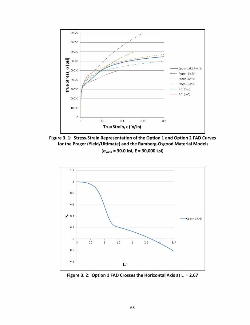
63

Figure 3. 1: Stress‐Strain Representation of the Option 1 and Option 2 FAD Curves for the Prager (Yield/Ultimate) and the Ramberg‐Osgood Material Models

(σyield = 30.0 ksi, E = 30,000 ksi)

Figure 3. 2: Option 1 FAD Crosses the Horizontal Axis at Lr = 2.67

64

Figure 3. 3: Stress Asymptote Associated with the (‐) and (+) Values of f1 (σyield = 30.0 ksi, E = 30,000 ksi)

Convention dictates that the reference stresses used in the calculation of the equivalent

mechanical reference strain from Eq. 2.25 and in turn the load combination factor ψ

from Eq 2.32 should not exceed 2.67 (σyield) so that invalid values of true stress are not

used from the upper branch of the bifurcated stress‐strain curve, as shown in Figure 3.3.

The ψ factors developed in this work are based on Option 2 FAD curves. Various

values of ψ based on materials typically employed for the manufacturing of pressure

vessels are compiled in Appendix A. These values were based on utilizing the Prager

[18] stress‐strain model. However, the methodology described in Chapter IV for

determining ψ is applicable to any stress‐strain relation.

65

CHAPTER IV ‐ MATERIAL SPECIFIC CORRECTION FACTORS ‐ Ψ2

4.1 Introduction

Historically the Option 1 FAD curve (f1) was developed as a lower bound to a

collection of material specific Option 2 FAD curves. Thus ψ factors that account for

secondary stresses that are based on the Option 1 FAD curve using a pseudo material

with an amalgamation of properties should produce similarly conservative failure

estimates. They do not always do so. The API/ASME Fitness‐for‐Service code, API‐579

[1], and the British structural integrity assessment procedures known as R6 [3] describe

the use of ψ1 factors. It will be shown later in the discussion that the Option 1 FAD

curve approach may or may not be conservative depending on the value of the primary

load ratio as well as the secondary load ratio. FAD curves for both Option 1 and Option

2 can cross one another for the same material at different primary load ratios in the

absence of secondary stresses. In addition, FAD curves for both options may shift above

or below one another depending on the value of the secondary load ratio. The use of

the Option 1 FAD curve does not always yield conservative answers. However, the

procedure developed originally by Ainsworth [14] and outlined in Chapter 2 is the

current industry norm and this approach utilizes the Option 1 FAD curve (f1) to generate

66

ψ factors. However, nothing precludes the use of an Option 2 FAD curve (f2) in the

computation of ψ factors, especially if this approach produces more conservative results

then the industry norm. In fact, if material properties are known, especially if stress‐

strain data is available up to and including the ultimate stress and its corresponding

strain, then there is no need for an Option 1 FAD curve approach. One can simply

perform an assessment using an Option 2 FAD curve in the presence of secondary

stresses.

In addition, the Option 2 FAD curves used to establish the lower bound for the

Option 1 FAD curve were constructed assuming that the materials being assessed follow

a Ramberg‐Osgood power law stress‐strain relationship. In this chapter that assumption

is relaxed and the stress‐strain relationships proposed by Prager and outlined in Chapter

3 will be used to compute Option 2 FAD curves (f2) and the corresponding ψ2 factors.

The difference between f1 using amalgamated properties and f2 using actual specific

properties, as well as differences associated with stress‐strain relationships are

generally depicted in Figure 4.1. Three curves are shown in this figure, i.e., an Option 1

FAD curve based on amalgamated material properties, an Option 2 FAD curve based on

the Prager stress‐strain relationship using actual material properties, and an Option 2

FAD curve based on the Ramberg‐Osgood stress‐strain relationship similarly using actual

material properties. The Option 2 curves in the figure are based on a material with a

yield strength of 25 ksi, an ultimate strength of 55 ksi and exclude the effects of

secondary stresses. Clearly both Option 2 FAD curves fall below the Option 1 FAD curve

for all primary load ratios ( PrL ) less than one. In addition, the Option 2 FAD curve

67

0

0.2

0.4

0.6

0.8

1

1.2

0 0.5 1 1.5 2

Kr

LrP

Option 1 (R6 Rev. 3)

Option 2 (Prager)

Option 2 (RBOG, n=10)

Figure 4. 1: Failure Assessment Diagrams ‐ Option 1 and Option 2

(yield = 25 ksi, ult = 55 ksi and E = 30,000 ksi)

derived using the Prager stress‐strain model lies below the Option 2 FAD curve derived

using the Ramberg‐Osgood stress‐strain relationship. This indicates that the Option 2

FAD curve (f2) developed using Prager’s stress‐strain relationship is the most

conservative of the three FAD curves for these material properties.

Whether or not the Prager stress‐strain law produces a more conservative failure

assessment for Option 2 FAD curves is dependent on the yield stress of the material and

the Ramberg‐Osgood hardening exponent. Option 2 FAD curves derived using the

Prager stress‐strain law produce more conservative failure estimates than the Option 1

FAD curve for materials with yield stresses below 40 ksi. Above 40 ksi yield stresses the

Prager based Option 2 FAD curves are no longer consistently the most conservative

option. However, if material properties are known then the conservatism offered by the

Option 1 FAD curve is not necessary. One should simply use actual material data when

68

in possession of this information. The work here assumes the design engineer has

access to this material data and the Prager stress‐strain law is used within the

framework developed by Ainsworth [14] for generating ψ factors.

The conservatism associated with each type of FAD curve was depicted in Figure

4.1. These curves did not include the effects of any secondary stresses have on the

failure assessment diagrams. Quantifying conservatism must be carefully considered

using ψ factors as outlined by Harrison et al. [3]. Keep in mind that the ψ2 factors

adjust the value of the stress intensity ratio, Kr. If an Option 1 FAD curve is used

1 1 1

1

1

( / )

P C Sref ref refP


f ff

(4.1)

and

1P S

r r rK K K (4.2)

Note that positive ψ1 factors effectively shift the Option 1 FAD curve down producing a

more conservative failure assessment, i.e., fitness for service is determined by

1rK f (4.3)

or

1 1P Sr rK K f (4.4)

If an Option 2 FAD curve is used then

2 2 2

2

1

( / )

P C Sref ref refP


f ff

(4.5)

and

2P S

r r rK K K (4.6)

69

i.e., fitness for service is determined by

2rK f (4.7)

or

2 2P Sr rK K f (4.8)

Thus one can’t simply track the differences in failure estimates of components subject

to secondary stress states by noting the differences in ψ1 and ψ2 for a specific

combination of load ratios LrS and Lr

P. The factor ψ1 is functionally dependent on f1 and

ψ2 is functionally dependent of f2. The effect from ψ1 factors on an Option 1 FAD curve

is depicted in Figure 4.2

0.000

0.200

0.400

0.600

0.800

1.000

1.200

0.0 0.2 0.4 0.6 0.8 1.0 1.2 1.4

Kr

LrP

Mechanical

Mechanical and Thermal

Ψ1(LrP,Lr

S)

ƒ1(LrP)

Figure 4. 2: Failure Assessment Diagrams with and without the Effects of ψ1

The effect from ψ2 factors on an Option 2 FAD curve is depicted in Figure 4.3. Since

each ψ factor affects a specific FAD curve, in order to compare values one must discern

the effect each ψ factor has on its respective FAD curve. Direct numerical comparison

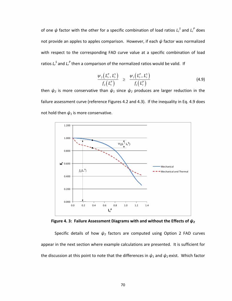
70

of one ψ factor with the other for a specific combination of load ratios LrS and Lr

P does

not provide an apples to apples comparison. However, if each ψ factor was normalized

with respect to the corresponding FAD curve value at a specific combination of load

ratios LrS and Lr

P then a comparison of the normalized ratios would be valid. If

2 1

2 1

, ,

P S P Sr r r r

P Pr r

L L L L

f L f L

(4.9)

then ψ2 is more conservative than ψ1 since ψ2 produces are larger reduction in the

failure assessment curve (reference Figures 4.2 and 4.3). If the inequality in Eq. 4.9 does

not hold then ψ1 is more conservative.

0.000

0.200

0.400

0.600

0.800

1.000

1.200

0.0 0.2 0.4 0.6 0.8 1.0 1.2 1.4

Kr

LrP

Mechanical

Mechanical and Thermal

Figure 4. 3: Failure Assessment Diagrams with and without the Effects of ψ2

Specific details of how ψ2 factors are computed using Option 2 FAD curves

appear in the next section where example calculations are presented. It is sufficient for

the discussion at this point to note that the differences in ψ1 and ψ2 exist. Which factor

71

produces a more conservative failure assessment will be pointed out as the discussion

unfolds.

4.2 Ainsworth’s Approach Using Option 2 FAD Curves

The first step in generating the material specific ψ2 factors using Option 2 FAD

curves is establishing the yield stress and the ultimate stress of material. In addition,

the primary and secondary stress states must be known. With this information one can

establish a reference strain. If the Option 2 approach is utilized, then a composite stress

can be computed using the reference strain and the Prager nonlinear stress‐strain

relationship discussed in the previous chapter. Once a composite stress value is

established a ψ2 factor can be computed using Eq. 4.5. If Ainsworth’s [14] approach is

used where an Option 1 FAD curve is used then Eq. 4.1 is employed and the composite

stress is computed using Eq. 2.24.

To establish a value for the composite stress σCref given a primary stress σPref and

a secondary stress σSref one must first establish a range for the dummy reference stress

σRref in order to compute a minimum reference strain. Noting that the sum of the

primary stress and the dummy reference stress is limited by the true ultimate stress of

the material, then

P Rref ref ultimate true

(4.10)

An upper bound can be established on the dummy reference stress with this expression,

i.e.,

R Pupper ref ultimate reftrue

(4.11)

72

A lower bound on the dummy reference stress can be surmised by noting that this

quantity appears in a denominator in Eq. 2.25, thus for practical purposes the lower

bound can be established at a value slightly larger than zero, say

0.001Rlower ref (4.12)

Given these values for an upper and lower limit on the dummy reference stress a series

of intermediate values can be established using

50Rref psi (4.13)

Incremental values of the dummy reference stress are computed using

max

max

1, 2, 3, ,R R Rref lower ref ref

i

R Rupper ref lower ref

Rref

i i i

i

(4.14)

The logic for adopting this value appears further in the discussion.

For each value of (σRref)i a corresponding reference strain value is computed

using Eq. 2.25 in the following form

22

2 22 2

1

( / )2

P Rref ref i

ref i P Rref ref yieldi

S R RSref ref refrefi i

SR Rref yieldref ref yieldi i

E f

f f

(4.15)

Note that in this equation

73

12 2

2 2

12 2

2

1

21

1

2 1

Sref

S Syieldref ref

S Syield ref ref

yield

SSrref

S Sref r

Ef

LE

L

(4.16)

As is evident in Figure 4.4 the function expressed in Eq. 4.15 produces a minimum along

the established range of dummy reference stresses. In this figure a material with a

Young’s modulus of 30,000 ksi, a yield stress of 30 ksi and an ultimate tensile

engineering strength of 60 ksi has been utilized. In this figure LrP was taken equal to

0.50, and LrS was equal to 1.50.

Figure 4. 4: Reference Strain vs. Dummy Reference Stress with (εref)min = 0.0738

yield = 30 ksi, ult = 60 ksi, E = 30,000 ksi, Lrp = 0.5, and Lr

S = 1.50)

74

One can hold the secondary stress ratio constant and vary the primary load ratio while

computing the minimum reference strain for each value of the primary load ratio. The

results from those computations are depicted in Figure 4.5 where the secondary load

ratio is equal to 1.50.

Figure 4. 5: (εref)min vs. LrP for an Option 2 FAD Curve Using Prager’s Stress‐Strain

Model

(yield = 30 ksi, ult = 60 ksi, E = 30,000 ksi, LrS = 1.50)

Clearly a minimum value for ref is established in Figure 4.4 within the range of

the dummy stress limits. Using this minimum value of ref a composite reference stress

is computed from Eq. 3.2 but solving for the stress, i.e.,

,min 1 2Cref refE (4.17)

where

11 1.0 tanh

2H

(4.18)

75

and

22 1.0 tanh

2H

(4.19)

Note that in the example where the minimum reference strain was determined to be

0.0738 the Prager stress‐strain constants are

30yield ksi (4.20)

60ultimate ksi (4.21)

0.5yield

ultimate

R

(4.22)

0.00002p (4.23)

0.002ys (4.24)

1

ln0.151

ln 1ln

ln 1

p ys

p

ys

Rm

(4.25)

2 0.60 1.00 0.3m R (4.26)

11

176,800

ln 1

yield ys

m

ys

A

(4.27)

2

22

2

exp116,000ultimate

m

mA

m

(4.28)

1.5 2.5 3.51.5 0.5 0.353K R R R (4.29)

The ultimate stress listed above is an engineering stress quantity and

76

2

2.29

Cref yield ultimate yield

uttimate yield

KH

K

(4.30)

Note that

1

1

11

0.0830C mref

A

(4.31)

and

22

2

1

0.0719Cref m

A

(4.32)

depend on the composite reference stress. Thus a value of the composite reference

must be found that satisfies Eq. 4.17, Eq. 4.30, Eq. 4.31 and Eq. 4.32 simultaneously

given the minimum reference strain and the Prager constants stipulated above. For

Figure 4. 6: σCref as a Function of Lr

P for Option 2 FAD Curves (Prager)

(yield = 30 ksi, ult = 60 ksi, and E = 30,000 ksi)

77

these material constants and the minimum value of ref depicted in Figure 4.4, the value

of the equivalent mechanical reference stress is 52.8 ksi. In Figure 4.6 the composite

reference stress is depicted as a function of the primary load ratio. The secondary load

ratio is equal to 1.5 in this figure.

Once the equivalent mechanical reference stress was determined, the ψ2 factor

can be computed from Eq. 4.5 when using the Option 2 FAD curve. Figure 4.7 depicts

the variation of ψ2 with the primary load ratio. The secondary load ratio is once again

equal to 1.5 in this figure. Note that the value of ψ2 approaches zero at a primary load

ratio nearly equal to one.

Figure 4. 7: ψ2 as a Function of LrP for Option 2 FAD Curves (Prager)

(yield = 30 ksi, ult = 60 ksi, and E = 30,000 ksi)

Earlier a value of 50 psi was used as the incremental value Δ Rref so that accurate

values for the minimum reference strain can be established. A number of calculations

78

were performed to determine this optimal value for Δ Rref and the results from this

effort are shown graphically in Figure 4.8. Here the dummy reference stress, Rref ,

associated with a computed minimum reference strain, ,minref , is graphed as a function

of the primary load ratio, PrL . The secondary load ratio was taken equal to 0.5, and the

value of Δ Rref was varied several times by an order of magnitude from curve to curve.

One can easily see that asymptotic behavior is obtained by the time Δ Rref reaches 50

psi. For computational efficiency this value of Δ Rref was utilized throughout this study.

Figure 4. 8: Resolution Study for the Dummy Reference Stress, σRref at (εref)min

(LrS = 0.5, yield = 30 ksi, ult = 60 ksi, E = 30,000 ksi, Ferritic Steel)

The corresponding ψ2 factors for this resolution study as a function of the primary load

ratio are shown in Figure 4.9. Each curve corresponds to a Δ Rref value used in Figure

4.8, i.e., comparisons were made between computations using Δ Rref values of 5000,

79

500, 50 psi to that of an analysis performed at 5 psi. In both figures it is clear that

asymptotic behavior is attained by the time Δ Rref is equal to 50 psi.

Figure 4. 9: ψ Values Corresponding to σRref Resolution Study

(LrS = 0.5, σyield = 30 ksi, σult = 60 ksi, E = 30,000 ksi, Material ‐ Ferritic Steel)

The minimum reference strain and the corresponding dummy reference stress

are functions of both the primary load ratio as well as the secondary load ratio. Up to

this point the effects in the variation associated with the primary load ratio have been

illustrated. In Figures 4.10, 4.11 and 4.12 variations in the minimum reference strain,

the composite reference stress, and ψ2 as functions of the primary load ratio are

presented with respect to secondary load ratios of 0, 0.5, 1.0, 1.5, and Lr max. It is

apparent in Figure 4.10 that the minimum reference strain increases with an increasing

secondary load ratio.

80

Figure 4. 10: (εref)min vs. LrP for Option 2 FAD Curves Using Prager’s Stress‐Strain Model

and Three Values of the Secondary Load Ratio

(σ yield = 30 ksi, σ ult = 60 ksi, and E = 30,000 ksi)

Figure 4. 11: σCref vs. Lr

P for Option 2 FAD Curves Using Prager’s Stress‐Strain Model

and Three Values of the Secondary Load Ratio


81

In a corresponding fashion, the composite reference stress increases with an increasing

secondary load ratio, which is depicted in Figure 4.11.

Finally in Figure 4.12 one can easily see that the absolute value of ψ2 decreases

for all values of the primary load ratio as the secondary load ratio decreases. In the

near vicinity of 1.0 for the primary load ratio all values of ψ2 approach zero irrespective

of the secondary load ratio.

Figure 4. 12: ψ as a Function of LrP for Option 2 FAD Curves

Using Prager’s Stress‐Strain Model and Three Values of the Secondary Load Ratio


4.3 A Comparison of Methods

In the previous section the methodology for computing the ψ2 factors based on

Option 2 FAD curves using the Prager stress‐strain model was presented with an

example. In this section general results are presented with comparisons made between

the methodologies presented in the previous section and the Option 1 FAD curve

82

approach as well as the Option 2 FAD curve approach to calculating ψ2 factors using the

Ramberg‐Osgood stress‐strain model.

Consider the plot of reference strain versus the dummy reference stress, Rref ,

for a material with a yield stress of 30 ksi, ultimate engineering stress of 60 ksi, primary

load ratio, PrL , equal to one, and a secondary load ratio, S

rL , equal to 0.01, which is

shown in Figure 4.13. Three curves appear in the figure along with the upper limit on

the dummy stress defined by Eq. 4.11. One curve is based on an Option 1 FAD curve,

the second and third curves are based on Option 2 FAD curves where the Prager stress‐

strain model and the Ramberg‐Osgood stress‐strain model with a hardening exponent of

10 are utilized, respectively. For very small values of the secondary load ratio the

secondary stress obviously approaches zero and the upper limit on the range for the

dummy reference stress will approach the value of the true ultimate stress minus

primary stress value. In this case the upper limit for the dummy reference stress is

grossly overestimated by the ultimate stress. Given the inequality in Eq. 4.10 the

minimum reference strain approaches the value of the first term in Eq. 4.15, that is,

22

1Pref

i Pref yield

E f

(4.33)

since the second term is multiplied by a factor that approaches zero as the secondary

stress approaches zero. Thus the composite stress approaches the primary stress, as it

should, and the ψ factor goes to zero, as it should.

Next a plot of reference strain versus dummy stress for the same material, same

primary load ratio but a secondary load ratio of 1.50 appears in Figure 4.14. Once again

83

Figure 4. 13: Reference Strain vs. Dummy Reference Stress

(yield = 30 ksi, ult = 60 ksi, E = 30,000 ksi, Lrp = 1, Lr

S = 0.01)


(yield = 30 ksi, ult = 60 ksi, E = 30,000 ksi, Lrp = 1, Lr

S = 1.5)

84

three curves are depicted in the figure based on the Option 1 FAD curve, and two based

on the Option 2 FAD curves using the Prager stress‐strain model and the Ramberg‐

Osgood stress‐strain model with a hardening exponent of 10, respectively. Note that

minimum values for the reference strain are clearly defined along each curve before the

upper limit of the dummy stress is attained.

Two trends are clearly evident in this figure and the ones that follow. First the

minimum reference strain associated with the Ramberg‐Osgood stress‐strain model

(n=10) is significantly larger than the minimum reference strain produced by the other

two curves. The minimum reference strain will increase proportionally with the

Ramberg‐Osgood exponent. The second trend is that minimum reference strain

associated with the Prager stress‐strain model is the intermediate value, and the

minimum reference strain associated with the Option 1 FAD curve produces the smallest

minimum reference strain and as a result the smallest composite stress, i.e., the least

conservative. Furthermore the Prager minimum reference strain using the Option 2 FAD

curve is much closer to the Option 1 FAD curve developed by Ainsworth [14]. However,

the Prager minimum reference strain remains more conservative. These two trends

continue in the next two figures.

A third plot of reference strain versus dummy stress for the same material as the

previous two figures, same secondary load ratio as the previous figure, but with a

primary load ratio of 0.01, appears in Figure 4.15. Again, the three curves depicted in

the figure are based on the Option 1 FAD curve, and two based on the Option 2 FAD

curves using the Prager stress‐strain model and the Ramberg‐Osgood stress‐strain

85

model with a hardening exponent of 10. As in the previous figure the minimum

reference strain associated with the Ramberg‐Osgood stress‐strain model is the largest

among the three curves. The minimum reference strain associated with the Prager

stress‐strain model is the intermediate value, and the minimum reference strain

associated with the Option 1 FAD curve produces the smallest minimum reference strain

and as a result the minimum composite stress.


(yield = 30 ksi, ult = 60 ksi, E = 30,000 ksi, Lrp = 0.01, Lr

S = 1.5)

A fourth plot of reference strain versus dummy stress for the same material,

same secondary load ratio as the previous figure, but a primary load ratio of 1.5 appear

in Figure 4.16. The three curves depicted in the figure are based on the Option 1 FAD

curve, and two based on the Option 2 FAD curves using the Prager stress‐strain model

and the Ramberg‐Osgood stress‐strain model with a hardening exponent of 10. Again,

the minimum reference strain associated with the Ramberg‐Osgood stress‐strain model

86

is the largest among the three curves. The minimum reference strain associated with

the Prager stress‐strain model is the intermediate value, and the minimum reference

strain associated with the Option 1 FAD curve produces the smallest minimum reference

strain and as a result the minimum composite stress.


(yield = 30 ksi, ult = 60 ksi, E = 30,000 ksi, Lrp = 1.50, Lr

S = 1.5)

As noted above, the minimum reference strain is converted to a composite

reference stress. The work here proposes the use of the Prager stress‐strain

relationship to make this conversion. Once a value of the composite stress is computed

a ψ2 factor is calculated using Eq. 4.5. Appendix A provides tabulated ψ2 factors, ψ2

curves, stress‐strain curves, and Option 2 FAD curves for a range of materials used in the

manufacturing of pressure vessels and sanctioned by ASME Section VIII, Division 1 and

2.

87

It is apparent that using the Option 1 FAD curve is not consistently the most

conservative approach. For instance, a comparison of the Option 2 FAD for ferritic

steels with a yield stress of 20 ksi and an ultimate engineering stress of 70 ksi to the

Option 1 FAD curve in Figure 4.17 indicates that the Option 1 FAD curve is non‐

conservative over most of its range. A similar comparison of the Option 1 FAD curve

with an Option 2 for ferritic steel with a yield stress of 70 ksi and ultimate engineering

stress of 90 ksi indicates that the Option 1 FAD curve is conservative for PrL values

greater than 0.7. These trends hold throughout Appendix A. In general, the Option 1

FAD curve is non‐conservative for materials with yield stresses below 40 ksi and

conservative relative to Option 2 FAD curves using the Prager stress‐strain relationship

for materials with yield stresses greater the 40 ksi. This should be expected since the

materials selected to construct the Option 1 FAD curve were austenitic steels with a

yield stress of approximately 40 ksi. A material with similar properties produces an

Option 2 FAD curve similar to the Option 1 FAD curve. The stress‐strain curve for this

material appears as Figure 15 in Milne [6].

Developing the ψ2 factors based on material specific FAD curves using the

approach of Ainsworth [14] requires that the secondary stress intensity factor adjusted

for crack tip plasticity, SJK , is equal to S

IK , i.e., the elastic stress intensity ratio for mode I

fracture. This assumption produces a certain level of conservatism in the analysis.

Hooton and Budden [20] originally pointed this out and they suggested a way to adjust

for this conservatism. Their factor approach is a function of the material specific FAD

curve and is similarly dependent on the yield and ultimate stress. The material specific

88

factor should be calculated along with the material specific ψ factor. Material specific

factors are included in Appendix A

Figure 4. 17: Failure Assessment Diagrams, Option 1 and Option 2

(yield = 20 ksi, ult = 45 ksi, E = 30,000 ksi, Ferritic Steel)

(yield = 70 ksi, ult = 90 ksi, E = 30,000 ksi, Ferritic Steel)

4.4 Modeling Primary and Secondary Stresses with Finite Element Analysis

Cold working, hot rolling, grinding, quenching treatments, welding and thermal

cutting all can induce residual stresses in a fabricated component. Residual stresses,

i.e., secondary stresses by the ASME code, produced by any of the fabrication processes

mentioned above will have an effect on the resulting FAD curve. In a somewhat

complex fashion secondary stresses affect the shape of the FAD curve based on primary

stresses alone. The development of ψ factors was an attempt to account for secondary

stresses and to correct for their effect on the FAD curve. The following two examples

89

illustrate the effect that secondary stresses have on a FAD curve and underscore the

necessity for a correction factor to account for its affects.

In the first case study a finite element analysis was conducted on a prismatic

beam with a center crack that was first subjected to an edge displacement normal to

the crack length. After the displacement was applied, a uniform stress was

subsequently applied along the upper edge of the beam producing flexural stresses. In

the second case study the prismatic beam was subjected to the uniform stress, but the

uniform displacement was not applied. A finite element analysis was similarly

conducted on the second case. Results for both analyses are presented in the following.

The beam geometry used in the finite element analyses is depicted in Figure

4.18. The beam thickness (t) is one inch, the length (L) is twelve inches, and the depth

of the beam (W) is one inch. A center edge crack with a length (a = 0.5 inches) is present

and is perpendicular to the bottom edge of the beam. Material properties include

Young’s Modulus, E = 30,000,000 psi, the yield stress, σyield = 30,000 psi, and the ultimate

engineering stress, σult = 55,000 psi. The relationship between engineering stress and

true stress is

truegengineerintrue exp (4.34)

Utilizing this relationship at ultimate stress values then

2exp( )true ultultm (4.35)

where m2 is a Prager [18] constant that represents the ultimate true strain. For ferritic

steel with (See Table 3.1)

Rm 160.02 (4.36)

90

and

30

0.5455

yield

ult

R

(4.37)

then

55 exp(0.28)

72

true ult

ksi

(4.38)

in this analysis.

Figure 4. 18: Beam Geometry and Load Applications

A finite element analysis was conducted using Abaqus, which is a commercially

available finite element analysis software algorithm. In the finite element analysis two

dimensional planar shell elements were utilized. Specifically eight node bi‐quadratic

reduced integration planar elements were employed throughout the entire mesh. A

focused (spider web) mesh was generated around the crack tip, which is evident in

Figure 4.19. Degenerate elements were used in the vicinity of the crack tip. These

elements have nodes that collapse on one side of the element at the crack tip. The

collapse mechanism produces duplicate nodes at the same point in the component that

numerically simulates the singularity that exists at the tip of a sharp crack.

91

The center node on the left edge of the bend specimen was constrained in both

the x‐ and y‐directions and left free to rotate. The center node on the right edge of the

bend specimen was constrained in the y‐direction by a boundary condition and in the x‐

direction by the applied displacement. These boundary constraints and mesh densities

were used for both examples.

Crack Location

Focused Mesh

Figure 4. 19: Finite Element Mesh

For the analysis in Case 1 an initial displacement of 0.0014 inches was applied to

the right edge of the specimen in the positive x‐direction. This displacement

corresponds to a secondary load ratio (LrS) of 0.4. Subsequent to the application of a

uniform displacement a uniform pressure of 340 psig was applied in the negative y‐

direction along the top surface of the specimen opposite the crack. Two separate

analyses were performed for Case 1, an elastic analysis and nonlinear stress‐strain

analysis.

92

The initial displacement applied in Step 1 of the elastic analysis caused a peak

elastic stress of 47,620 psi at the crack tip using a linear stress‐strain relationship. The

addition of the uniform pressure in the second step caused the elastic peak stress to rise

to 300,200 psi. Peak stresses from the application of both boundary conditions were

well above the yield stress of the material. The von Mises stress is depicted in Figure

4.20 for the combined boundary conditions, i.e., the applied displacement and the

applied uniform pressure.

Pressure

Displacement

Elastic Case 1

Step 1:

Step 2:

Figure 4. 20: Case 1, Elastic

The stress‐strain relationship used for the nonlinear stress‐strain analysis was

based on Prager’s [18] stress‐strain relationship described in Chapter 3. Recall that this

constitutive relationship includes a strain hardening mechanism that permits the stress‐

strain curve to become nonlinear as the material is loaded. The material parameters

used in Prager’s [18] relationship includes information relative to the yield stress, the

93

ultimate stress, and Young’s modulus. In addition, the material was assumed to be a

ferritic steel with the Prager [18] constant m2 taken equal to 0.27, and εp was taken

equal to 2x10‐5. The initial displacement applied in Step 1 of the nonlinear stress‐strain

analysis produced a peak stress of 31,490 psi at the crack tip. The added uniform

pressure produced a total peak stress of 71,180 psi. The von Mises stress for the

nonlinear stress‐strain stress analysis is shown in Figure 4.21.

Pressure

Displacement

Elastic-Plastic Case 1

Step 1:

Step 2:

Figure 4. 21: Case 1, Elastic‐Plastic

The mechanical loads applied in Case 2 are the same as Case 1 with the

exception that no initial displacement was imposed in the analysis. The linear elastic

stress‐strain relationship and the nonlinear stress‐strain relationship used in Case 1

were adopted and used in Case 2.

When only the uniform pressure is applied the linear elastic peak stress was

94

Pressure

Elastic Case 2

Step 1:

Step 2:

Figure 4. 22: Case 2, Elastic

Pressure

Elastic-Plastic Case 2

Step 1:

Step 2:

Figure 4. 23: Case 2, Elastic‐Plastic

95

252,700 psi at the crack tip. The von Mises stress for this analysis is depicted in Figure

4.22.

When the nonlinear stress‐strain analysis was conducted for the uniform

pressure boundary condition a peak stress of 70,650 psi was produced at the crack tip.

The von Mises stress for the nonlinear stress‐strain stress analysis is shown in Figure

4.23. A summary of peak stresses developed for each case is shown in Table 4.1.

Table 4.1 Peak Stress From Finite Element Analyses

Case #1 Combined Displacement and Uniform Distributed load

Linear Elastic Nonlinear Stress‐Strain

Displacement Imposed

Displacement and Uniform Distrib. Load

Displacement Imposed

Displacement and

Uniform Distrib. Load

47,620 psi 300,200 psi 31,490 psi 71,180 psi

Case #2 Uniform Distributed load

Linear Elastic Nonlinear Stress‐Strain

Uniform Distributed Load Top Edge Uniform Distributed Load Top Edge

252,700 psi 70,650 psi

In the elastic analysis of Case 1 the stresses from the initial displacement and

subsequent applied pressure are additive. In the nonlinear stress‐strain analysis of Case

1 the stresses are not additive since the material hardens and the stress fields are

nonlinear. This is clearly evident when comparing the results of the nonlinear stress‐

strain analyses of Case 1 and Case 2. Stresses above yield are indicated as grey in the

contour plots for both load curves. Material hardening is indicated by the large portion

of the specimen identified with stresses above yield.

96

The uniform distributed load applied in both Case 1 and Case 2 was applied in

increments of 4 psi. The J‐integral was calculated for each increment. The J‐integral

results for Case 1 are shown in Figure 4.24. The effects of the secondary stress due to

the initial displacement applied in Step 1 of the analysis can be seen in Figure 4.24

where the initial value of the J‐integral was greater than zero. The J‐integral results for

Case 2 are shown in Figure 4.25. Note that as before Jtotal is the sum of Jelastic and Jplastic.

A comparison of the total J‐integrals for both Case 1 and Case 2 is shown in

Figure 4.26. As the applied load in Step 2 increased the total J‐integrals initially

increased at different rates, however as the applied load increased further the two

curves took on the same rate or growth.

Figure 4. 24: J‐integrals Case 1

97

Figure 4. 25: J‐integrals Case 2

Figure 4. 26: Total J‐integral for Case 1 and Case 2

98

The FAD curves for Case 1 and Case 2 are shown in Figure 4.27. The FAD curve

was calculated for each case by plotting totalelasticr JJK as a function of Lr PPL

Here P is the applied pressure and PL is the limit load for this specimen, i.e., PL = 203

psig. The limit load was determined by applying elastic‐perfectly plastic material

properties with a yield stress of 30 ksi to the specimen and increasing the applied load P

until the FEA solution would not converge. This simulates failure by plastic collapse.

Figure 4. 27: FAD Curves for Case 1 and Case 2

The differences between the two FAD curves in Figure 4.27 show the effects of

secondary stress. The FAD curve for Case 1 includes secondary stress. At lower Lr values

the larger values of the total J‐integral for Case 1 caused the FAD to drop below that of

the Case 2. As Lr increased further the Case 1 FAD began to approach the Case 2 FAD.

As Lr increased further the Case 1 FAD curve increased beyond that of Case 2 due to the

inclusion of the secondary stress in the calculation of Jelastic.

99

The results from the two examples indicate that secondary stresses have a

significant effect on the shape of the FAD curve. A FAD assessment must consider the

effects of secondary stress. One option is to create a specific FAD for each application

of secondary stress. This option would make a FAD assessment cumbersome and time

consuming. An alternative is to account for the effects of secondary stress though a

correction factor. Ainsworth [14] accomplished this by developing the ψ factor. The use

of the ψ factor enables the analyst to use one FAD for an analysis regardless of the level

of secondary stresses applied.

4.5 API‐579‐1/ASME FFS‐1 Part 9 Addendum

The material specific ψ2 values developed in this thesis are readily calculated for

a given load condition. The steps required to calculate ψ2 and φ2 should be included in

API‐579 [1] Part 9. The following steps are suggested as an addendum to API‐579 [1]

Part 9 paragraph 9.4.4.1 b. Steps 4 and 5 in this paragraph of API‐579 [1] should be

replaced by the following:

“Step 4 – Calculate the material specific ψ2 and φ2 factor using the following procedure:

a.) Determine the minimum reference strain, ε(σref)min, for a range of dummy

reference stresses, σRref , using the following equation and the material

specific FAD function of STEP 3, f2, where LrP = σPref/σy.

2 222 22

( ) ( )( )

2 ( / ) ( / )( ) /

P R S R S Rref ref ref ref ref ref

ref R S RP Rref ref yield ref yieldref ref yield Ef EfEf

Let σRref range in value from one to (σtrue, uts ‐ σPref). Increments for σRref

within this range should be set at a maximum of 50 psi.

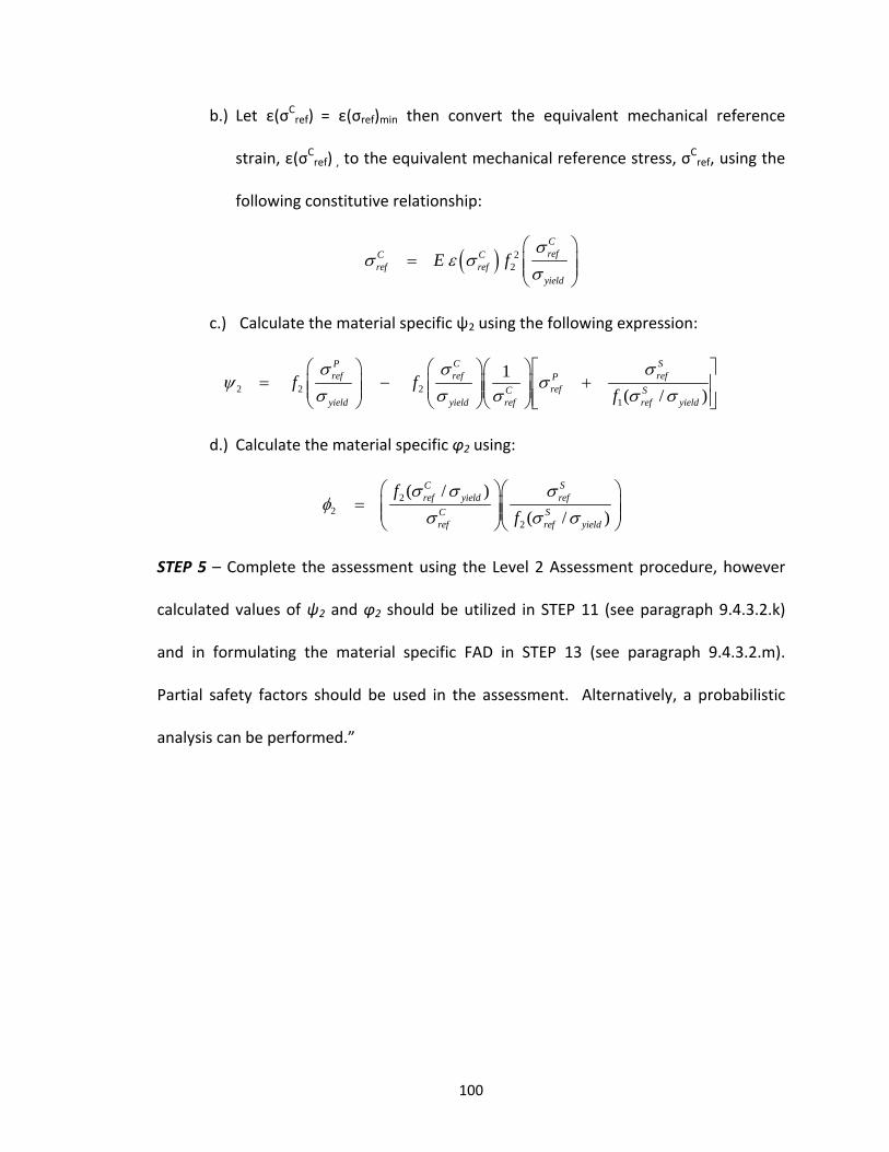
100

b.) Let ε(σCref) = ε(σref)min then convert the equivalent mechanical reference

strain, ε(σCref) , to the equivalent mechanical reference stress, σCref, using the

following constitutive relationship:

22

CrefC C

ref refyield

E f

c.) Calculate the material specific ψ2 using the following expression:

2 2 21

1

( / )

P C Sref ref refP


f ff

d.) Calculate the material specific φ2 using:

22

2

( / )

( / )

C Sref yield ref

C Sref ref yield

f

f

STEP 5 – Complete the assessment using the Level 2 Assessment procedure, however

calculated values of ψ2 and φ2 should be utilized in STEP 11 (see paragraph 9.4.3.2.k)

and in formulating the material specific FAD in STEP 13 (see paragraph 9.4.3.2.m).

Partial safety factors should be used in the assessment. Alternatively, a probabilistic

analysis can be performed.”

101

CHAPTER V ‐ PARAMETER SENSITIVITY ANALYSIS

5.1 Introduction

A study was conducted to evaluate the sensitivity of ψ2 factors to changes in the

parameters it depends on. The analyses included variations in yield stress and elastic

modulus. Later in the chapter changes in the type of material and the effect it has on ψ2

factors are explored. Sensitivity is quantified through a “residual” or a difference in the

value calculated without a variation in the parameter. Residuals are defined as

*2 2Residual , ,P S P S

r r r ri iL L L L (5.1)

Where *2 represents a value generated using a parameter that has been changed

percentagewise by 1%5%10% and 15%. The results from each analysis can be

presented in terms of “normalized residuals” one of which is defined as

*

2 2

2

, ,Percent Residual 100%

,

P S P Sr r r ri i

P Sr r i

L L L L

L L

(5.2)

This normalized residual is simply a percent residual. The residual defined in Eq. 5.1 can

also be normalized with respect to the Option 2 curve value (f2). The curve value is

associated with the unchanged parameters, and the relationship is expressed as

102

*

2 2

2

, ,Percent Normalized Residual 100%

P S P Sr r r ri i

Pr i

L L L L

f L

(5.3)

Normalized results provide a sense of the impact that a modified input parameter has

on a material specific Option 2 FAD curve analysis. The results provided include the

maximum and minimum residuals as well as the average residual over a range of

primary and secondary load ratios from zero to ( PrL )max and (

SrL )max, respectively, in

increments of 0.1. This is done for each percentage change in input parameter. The

quantities that appear in the equations above, i.e., 2 , *2 , and the corresponding

value of f2 the residual is normalized with, are identified in Figure 5.1.

Ψ2(LrP,Lr

S)i

f2*(LrP)i

Ψ2*(Lr

P,LrS)i Option 2 FADs

f2(LrP)i

Figure 5. 1: Graphical Representation of ψ2, ψ2* and the Option 2 Function (f2)

103

5.2 Yield Stress Sensitivity

The yield stress sensitivity analysis compared ψ2 factors calculated at a 30 ksi

yield stress to calculated values of ψ*2 associated with a 1% (yield = 29.7 ksi, yield =

30.3 ksi)a5% (yield = 28.5 ksi, yield = 31.5 ksi)a10% (yield = 27 ksi, yield = 33 ksi)

and a 15% (yield = 25.5 ksi, yield = 34.5 ksi) variation in this yield stress value. As was

just noted ψ2, and ψ*2 were computed over a range of primary and secondary load

ratios from zero to ( PrL )max and (

SrL )max, respectively, in increments of 0.1. This range

allows the computation of a maximum normalized residual, a minimum normalized

residual, and the average normalized residual over the entire range of the load ratio

increments. The maximum ψ2 at each secondary load ratio increment are plotted as a

function of Sr

Sr LfL 2 in Figures 5.2 (negative percent changes in the yield stress) and

Figure 5.3 (positive percent changes in the yield stress). As the yield stress was varied

the elastic modulus and the ultimate tensile strength were held at 30,000 ksi and 60 ksi,

respectively. The material hardening parameters for this ferritic steel are listed in Table

3.1.

Using Eq. 5.2 the largest average percentage change in the residual for ψ2 was

+23.6% and this value occurred at the +15% change in yield stress, i.e., yield = 34.5 ksi.

For a ‐15% change in yield stress, i.e., yield = 25.5 ksi, the average percentage change in

the residual for ψ2 was ‐9.1%. Results for all percent residuals are summarized in Table

5.1. Using Eq. 5.3 the largest average normalized change in the residual for ψ2 was

‐0.9% and this value occurred at the ‐15% change in yield stress. For a +15% change in

104

Figure 5. 2: Max ψ2 Factors as a Function of Load Ratio Normalized with Respect to f2

Corresponding to ‐1%, ‐5%, ‐10% and ‐15% Changes in Yield Stress

(Baseline yield = 30 ksi, E = 30,000 ksi, ult = 60 ksi, Ferritic Steel)

Figure 5. 3: Max ψ2 Factors as a Function of Load Ratio Normalized with Respect to f2 Corresponding to +1%, +5%, +10% and +15% Changes in Yield Stress


105

Table 5. 1: Yield Stress Sensitivity ‐ % Residuals


Statistic Yield Stress Differential (∆σyield)

‐15% ‐10% ‐5% ‐1% 1% 5% 10% 15%

Max 1456.7 947.7 464.5 95.0 458.5 2350.6 4849.4 7504.0

Min ‐6455.8 ‐4391.9 ‐2248.2 ‐452.7 ‐95.9 ‐484.4 ‐995.9 ‐1538.4

Mean ‐9.1 ‐6.4 ‐3.4 ‐0.7 0.9 4.7 10.4 23.6

Table 5. 2: Yield Stress Sensitivity ‐ % Normalized Residuals


Statistic Yield Stress Differential (∆σyield)

‐15% ‐10% ‐5% ‐1% 1% 5% 10% 15%

Max 10.9 7.5 3.8 0.8 0.6 3.2 6.4 9.6

Min ‐9.1 ‐6.1 ‐3.1 ‐0.6 ‐0.8 ‐4.0 ‐8.1 ‐12.4

Mean ‐0.9 ‐0.5 ‐0.2 0.0 0.0 0.2 0.3 0.6

yield stress the average normalized change in the residual ψ2 was +0.6%. Results for all

the percent normalized residuals are summarized in Table 5.2.

Maximum ψ2 factors as a function of Sr

Sr LfL 2 for the ‐1% change in yield

stress (yield = 29.7 ksi), the ‐5% change in yield stress (yield = 28.5 ksi),the10% change

in yield stress (yield = 27 ksi), and the ‐15% change in yield stress (yield = 25.5 ksi) are

provided in Figure 5.2. Maximum ψ2 factors as a function of Sr

Sr LfL 2 for the +1%

change in yield stress (yield = 30.3 ksi), the +5% change in yield stress (yield = 31.5

ksi),the10% change in yield stress (yield = 33 ksi), and the +15% change in yield stress

(yield = 34.5 ksi) are provided in Figure 5.3. Units along the horizontal axis are

historically consistent with the original development of ψ. The reader is directed to

Figure 5 in Ainsworth [14].

106

Percent residuals (Eq. 5.2) as a function of SrL for the ‐1% change in yield stress

(yield = 29.7 ksi), the ‐5% change in yield stress (yield = 28.5 ksi),the10% change in

yield stress (yield = 27 ksi), and the ‐15% change in yield stress (yield = 25.5 ksi) are

provided in Figure 5.4. Percent residuals (Eq. 5.2) as a function of SrL for the +1%

change in yield stress (yield = 30.3 ksi), the +5% change in yield stress (yield = 31.5

ksi),the10% change in yield stress (yield = 33 ksi), and the +15% change in yield stress

(yield = 34.5 ksi) are provided in Figure 5.5.

Figure 5. 4: Percent Residuals as a Function of the Secondary Load Ratio Corresponding to ‐1%, ‐5%, ‐10% and ‐15% Changes in Yield Stress


107

Figure 5. 5: Percent Residuals as a Function of the Secondary Load Ratio Corresponding to +1%, +5%, +10% and +15% Changes in Yield Stress


Figure 5. 6: Percent Normalized Residuals as a Function of the Secondary Load Ratio Corresponding to ‐1%, ‐5%, ‐10% and ‐15% Changes in Yield Stress


108

Percent normalized residuals (Eq. 5.3) as a function of SrL for the ‐1% change in

yield stress (yield = 29.7 ksi), the ‐5% change in yield stress (yield = 28.5 ksi),the10%

change in yield stress (yield = 27 ksi), and the ‐15% change in yield stress (yield = 25.5

ksi) are provided in Figure 5.6. Percent normalized residuals (Eq. 5.3) as a function of

SrL for the +1% change in yield stress (yield = 30.3 ksi), the +5% change in yield stress

(yield = 31.5 ksi),the10% change in yield stress (yield = 33 ksi), and the +15% change in

yield stress (yield = 34.5 ksi) are provided in Figure 5.7.

Figure 5. 7: Percent Normalized Residuals as a Function of the Secondary Load Ratio Corresponding to +1%, +5%, +10% and +15% Changes in Yield Stress

(Baseline σyield = 30 ksi, E = 30,000 ksi, σult = 60 ksi, Ferritic Steel)

5.3 Elastic Modulus Sensitivity

The sensitivity analysis with respect to Young’s modulus compared ψ2 factors

calculated at with a Young’s modulus (E) of 30,000 ksi to calculated values of ψ*2

associated with a 1% (= 29,700 ksi, = 30,300 ksi)a5% (= 28,500 ksi, =

109

31,500 ksi)a10% (= 27,000 ksi, = 33,000 ksi) and a 15% (= 25,500 ksi, =

34,500 ksi) variation in this Young’s modulus value. As in the last section ψ2, and ψ*2

were computed over a range of primary and secondary load ratios from zero to ( PrL )max

and ( SrL )max, respectively, in increments of 0.1. This range allows the computation of a

maximum normalized residual, a minimum normalized residual, and the average

normalized residual and a percentage change over the entire range of the load ratio

increments. The maximum ψ2 at each secondary load ratio increment are plotted for

comparison in Figures 5.8 (negative percent changes in the Young’s modulus) and Figure

5.9 (positive percent changes in the Young’s modulus). As the elastic modulus is varied

yield stress and the ultimate tensile strength were held at 30 ksi and 60 ksi, respectively.

The material hardening parameters for this ferritic steel are the same as the last section

and they can be found in Table 3.1.

Using Eq. 5.2 the largest average percentage change in the residual for ψ2 was

‐4.3% and this value occurred at the ‐15% change in Young’s modulus, i.e., = 25,500

ksi. For a +15% change in Young’s modulus, i.e., = 34,500 ksi, the average percentage

change in the residual for ψ2 was ‐1.6%, and this was not the second highest percentage

change. That took place at the ‐10% change in Young’s modulus, i.e., = 27,000 ksi

where the average percentage change in residuals was ‐2.6%. Results for all percent

residuals are summarized in Table 5.3. Using Eq. 5.3 the largest average normalized

change in the residual for ψ2 was +0.8% and this value occurred at the ‐15% change in

Young’s modulus. For a +15% change in Young’s modulus the average normalized

110

Figure 5. 8: Max ψ2 Factors as a Function of Load Ratio Normalized with Respect to f2 Corresponding to ‐1%, ‐5%, ‐10% and ‐15% Changes in Young’s Modulus

(yield = 30 ksi, Baseline E = 30,000 ksi, ult = 60 ksi, Ferritic Steel)

Figure 5. 9: Max ψ2 Factors as a Function of Load Ratio Normalized with Respect to f2 Corresponding to +1%, +5%, +10% and +15% Changes in Young’s Modulus


111

Table 5. 3: Young’s Modulus Sensitivity ‐ % Residual


Statistic Modulus Differential (∆E)

‐15% ‐10% ‐5% ‐1% 1% 5% 10% 15%

Max 2208.2 1469.3 707.3 147.3 48.7 240.1 472.0 418.0

Min ‐771.4 ‐505.5 ‐248.4 ‐49.0 ‐117.6 ‐693.7 ‐1362.8 ‐1976.2

Mean ‐4.3 ‐2.6 ‐1.3 ‐0.2 0.3 0.8 1.5 ‐1.6

Table 5. 4: Young’s Modulus Sensitivity ‐ % Normalized Residuals


Statistic Modulus Differential (∆E)

‐15% ‐10% ‐5% ‐1% 1% 5% 10% 15%

Max 5.5 3.5 1.7 0.3 0.0 0.2 0.4 0.6

Min ‐0.7 ‐0.5 ‐0.2 0.0 ‐0.3 ‐1.5 ‐3.0 ‐4.0

Mean 0.8 0.5 0.2 0.0 0.0 ‐0.2 ‐0.4 ‐0.5

change in the residual ψ2 was ‐0.5%. Results for all the percent normalized residuals are

summarized in Table 5.4.

Maximum ψ2 factors as a function of Sr

Sr LfL 2 for the ‐1% change in Young’s

modulus (E = 29,700 ksi), the ‐5% change in Young’s modulus ( = 28,500 ksi),the10%

change in Young’s modulus ( = 27,000 ksi), and the ‐15% change in yield stress ( =

25,500 ksi) are provided in Figure 5.8. Maximum ψ2 factors as a function of Sr

Sr LfL 2

for the +1% change in Young’s modulus ( = 30,300 ksi), the +5% change in Young’s

modulus ( = 31,500 ksi),the10% change in Young’s modulus ( = 33,000 ksi), and

the +15% change in Young’s modulus ( = 34,500 ksi) are provided in Figure 5.9.

112

Percent residuals (Eq. 5.2) as a function of SrL for the ‐1% change in Young’s

modulus (E = 29,700 ksi), the ‐5% change in Young’s modulus ( = 28,500 ksi),the10%

change in Young’s modulus ( = 27,000 ksi), and the ‐15% change in Young’s modulus

( = 25,500 ksi) are provided in Figure 5.10. Percent residuals (Eq. 5.2) as a function of

SrL for the +1% change in Young’s modulus ( = 30,300 ksi), the +5% change in Young’s

modulus ( = 31,500 ksi),the10% change in Young’s modulus ( = 33,000 ksi), and

the +15% change in Young’s modulus ( = 34,500 ksi) are provided in Figure 5.11.

Figure 5. 10: Percent Residuals as a Function of the Secondary Load Ratio Corresponding to ‐1%, ‐5%, ‐10% and ‐15% Changes in Young’s Modulus


113

Figure 5. 11: Percent Residuals as a Function of the Secondary Load Ratio Corresponding to +1%, +5%, +10% and +15% Changes in Young’s Modulus


Percent normalized residuals (Eq. 5.3) as a function of SrL for the ‐1% change in

Young’s modulus (E = 29,700 ksi), the ‐5% change in Young’s modulus ( = 28,500

ksi),the10% change in Young’s modulus ( = 27,000 ksi), and the ‐15% change in

Young’s modulus ( = 25,500 ksi) are provided in Figure 5.12. Percent normalized

residuals (Eq. 5.3) as a function of SrL for the +1% change in Young’s modulus ( =

30,300 ksi), the +5% change in Young’s modulus ( = 31,500 ksi),the10% change in

Young’s modulus ( = 33,000 ksi), and the +15% change in Young’s modulus ( =

34,500 ksi) are provided in Figure 5.13.

114

Figure 5. 12: Percent Normalized Residuals as a Function of the Secondary Load Ratio Corresponding to ‐1%, ‐5%, ‐10% and ‐15% Changes in Young’s Modulus


Figure 5. 13: Percent Normalized Residuals as a Function of the Secondary Load Ratio Corresponding to +1%, +5%, +10% and +15% Changes in Young’s Modulus


115

5.4 A Comparison of Ferritic Steel With Other Metal Alloys

The material sensitivity analysis compared ψ2 factors calculated using hardening

parameter based on ferritic steel to those calculated using stainless steel and nickel

alloys, duplex stainless steel, and precipitation hardened nickel hardening parameters.

The material parameters that were varied were m2 and εp from Table 3.1. The

parameters that were held constant in the analyses were the yield stress at 30 ksi, the

ultimate stress at 60 ksi, and modulus at 30,000 ksi.

The results indicated an average residual of ‐0.4% for a stainless steel and nickel

alloy comparison, ‐0.3% for a duplex stainless steel comparison, and 33.5% difference

for a precipitation hardened nickel comparison. The average normalized residuals were

‐0.3% for a stainless steel and nickel alloy comparison, ‐0.1% for a duplex stainless steel

comparison, and ‐3.9% for a precipitation hardened nickel comparison. The results for

the comparison of ferritic steel with stainless steel and nickel alloy are summarized in

Table 5.5. The results for the comparison of ferritic steel with duplex stainless steel are

summarized in Table 5.6. The results for the comparison of ferritic steel with

precipitation hardened nickel are summarized in Table 5.7. Graphs depicting the

maximum ψ2 factors versus Sr

Sr LfL 2 for all material comparisons are shown in Figure

5.14. Graphs depicting the percent change in residual from Eq. 5.2 as a function of

SrL for all material comparisons, i.e., ferritic steel with stainless steel and nickel alloys,

ferritic steel with duplex stainless steel, and ferritic steel with precipitation hardened

nickel are shown in Figure 5.15. Graphs depicting the normalized residual from Eq. 5.3

as a function of SrL for all three material comparisons are shown in Figure 5.16.

116

Table 5. 5: Material Sensitivity Results, Ferritic Steel vs. Stainless Steel and Nickel Alloys

(yield = 30 ksi, E = 30,000 ksi, ult = 60 ksi)

Function % Residual % Normalized Residual

Max 334.9 2.8

Min ‐305.3 ‐10.3

Mean ‐0.4 ‐0.3

Table 5. 6: Material Sensitivity Results, Ferritic Steel vs. Duplex Stainless Steel

(yield = 30 ksi, E = 30,000 ksi,ult = 60 ksi)


Max 101.4 0.6

Min ‐85.2 ‐2.5

Mean ‐0.3 ‐0.1

Table 5. 7: Material Sensitivity Results, Ferritic Steel vs. Precipitation Hardened Nickel

(yield = 30 ksi, E = 30,000 ksi,σult = 60 ksi)


Max 3928.0 11.2

Min ‐3904.7 ‐74.4

Mean 33.5 ‐3.9

117

Figure 5. 14: Material Sensitivity ‐ Maximum ψ2 Factor


Figure 5. 15: Material Sensitivity – Percent Residual


118

Figure 5. 16: Material Sensitivity – Percent Normalized Residual


119

CHAPTER VI ‐ SUMMARY AND CONCLUSIONS

The ψ factor approach to account for the secondary stress effect developed by

Ainsworth [14] is based on the concept of an equivalent mechanical load that produces

the same value of the J‐integral as the combined load. Primary and secondary loads are

not additive outside the linear elastic range. The load combination factor allows for the

inclusion of secondary stresses into a FAD assessment. Ainsworth’s development of the

ψ factor allows for an equivalent mechanical reference stress to be formulated in such a

way that it can be easily incorporated into the methodologies of the fitness‐for‐service

Codes without defining a new version of the FAD. Inclusion of the effects of secondary

stress is accomplished by simply adding the ψ factor to the sum of the primary and

secondary stress intensity ratios.

The rationale for choosing the Option 1 FAD curve for assessments is

diminishing. The assumption that it is a conservative option is rarely correct when using

materials that do not conform to a power law model. For materials that do conform to

a power law model, the conservatism is only applicable when PrL < 1. In addition, since

the Option 1 FAD curve is a lower bound fit and not based on an actual material, the

120

non‐conservative region beyond PrL = 1 has no basis or meaning. The availability and

ease of generating Option 2 FAD curves using simple spreadsheets makes it a viable

option over the Option 1 FAD curve. These reasons suggest that the Option 1 FAD curve

should be used in a limited fashion and in its place the Option 2 FAD curve should be

used in assessments where material property data is available and generation of the J

integrals through advanced analysis is not practical.

Stress‐strain relationships deemed more realistic than those of a simple power

law (Ramberg‐Osgood) are allowed by the ASME Code [17]. This suggests the need for

unique ψ factors. The work in this thesis has shown that Option 1 FAD curve once

considered a conservative option is now in many cases non‐conservative. The use a

single set of ψ factors for all FAD curves appears short sighted from the perspective of

the design engineer. Data presented in Appendix A identifies the material specific ψ‐

factors to be used in conjunction with the material specific Option 2 FAD curves.

Derivation of material specific ψ factors has been performed using the same methods

established by Ainsworth [14] to generate the Option 1 ψ factors. Errors associated

with uncertainties in input data are small.

In this work it was pointed out that the units associated with the published

values of ψ and φ in the American Petroleum Institute (API) Fitness‐for‐Service Code

(API‐579) [1] are incorrect. These incorrect units lead users to select non‐conservative

values for each of these factors. The errors may be corrected by replacing the

121

horizontal axis labels SrL in appropriate tables with the correct axis labels

/ S Sr rL f L or by converting the current values to the equivalent S

rL values.

The development presented in thesis was based on earlier work by Ainsworth

[14], and was not intended to validate his results but to expand on them. Further work

regarding the material specific ψ factor may include finite element analysis to support

the results of this thesis. In addition, benefit may be gained by the derivation of a

single formula for the material specific ψ factor base on the parameters used in its

development.

122

BIBLIOGRAPHY

1. “API 579‐1/ASME FFS‐1 Fitness‐for‐Service,” American Petroleum Institute,

Washington, DC, 2007

2. “The effect of Defects on Structural Failure: A Two‐Criteria Approach,” A.R. Dowling

and C.H.A. Townley, International Journal of Pressure Vessels & Piping, Vol. 3, No.

2, pp 77‐107, 1975

3. “Assessment of the Integrity of Structures Containing Defects,” R.P. Harrison, K.

Loosemore, and I. Milne, CEGB Report No. R/H/R6, Central Electric Generating

Board, London, UK, 1976.

4. “Failure Assessment Diagrams for Use In R6 Assessments for Austenitic

Components,” R.A. Ainsworth, International Journal of Pressure Vessels and

Piping, Vol. 65, pp. 303‐309, 1996.

5. “Ductile Fracture Handbook,” A.Zahoor, EPRI Report NP‐6301‐D, Electric Power

Institute, Palo Alto, California, 1989.

6. “The Assessment of Defects in Structures of Strain Hardening Materials,” R.A.

Ainsworth, Engineering Fracture Mechanics, Vol. 19, No. 4, pp. 633‐642, 1984.

7. “Yielding in Steel Sheets Containing Slits,” D.S. Dugdale, Journal of the Mechanics

and Physics of Solids, Vol. 8, pp. 100‐104, 1960.

8. “Fully Plastic Crack Solutions, Estimation Scheme and Stability Analysis for the

Compact Specimen,” V. Kumar and C.F. Shih, ASTM‐STP 700 Fracture Mechanics,

P.C. Paris (ed.), pp.406‐438, 1980.

123

9. “The Penny‐Shaped Crack and the Plain‐Strain Crack in an Infinite Body of Power‐

Law Material,” M.Y. He and J.W. Hutchinson, Journal of Applied Mechanics, Vol.

48, 1981, pp. 830‐840.

10. “Description of Stress‐Strain Curves by Three Parameters,” W. Ramberg and W.R.

Osgood, National Advisory Committee for Aeronautics, Washington, DC , 1943.

11. Fracture Mechanics: Fundamentals and Application, T.L. Anderson, CRC Press,

2005.

12. “Assessment of the Integrity of Structures Containing Defects,” R.P. Harrison,K.

Loosemore, I. Milne, UK Central Electric Generating Board, CEGB Report No.

R/H/R6, Revision 4, 1976

13. “Backgound to and Validation of CEGB Report R/H/R6 ‐ Revision 3,” I. Milne, R.A.

Ainsworth, A.R. Dowling and A.T. Stewart, International Journal of Pressure Vessels

& Piping, Vol. 32, pp. 105‐196, 1988.

14. “The Treatment of Thermal and Residual Stresses in Fracture Assessments,” R.A.

Ainsworth, Engineering Fracture Mechanics, Vol. 24, pp. 65‐76, 1986.

15. “Further Developments of a J‐Based Design Curve and its Relationship to Other

Procedures ,“ C.E. Turner, in Elastic‐Plastic Fracture, ASTM STP 803, II.80‐II.102

(1983).

16. “A Procedure for Incorporating Thermal and Residual Stresses into the Concept of a

Failure Assessment Diagram,” G.G. Chell, ASTM STP‐668 Elastic‐Plastic Fracture, J.

D. Landes , J. A. Begley and G. A. Clarke Eds., pp. 581‐605, 1979,.

17. ASME Boiler and Pressure Vessel Code (SI), ASME, Section VIII, Division 2, 2007

18. ASME Boiler and Pressure Vessel Code (SI), ASME, Section VIII, Division 2, Annex

3D, 2007

19. “Bounding Structural Deformation due to Combined Creep and Plasticity,” R.A.

Ainsworth, 1980, U.K.: Central Electric Generating Board.

20. “R6 Developments in the Treatment of Secondary Stresses,” D.G. Hooton and P.J.

Budden, Fatigue and Fracture Mechanics in Pressure Vessels and Piping, ASME

PVP Vol. 304, pp. 503‐509, 1995.

21. ASME Boiler and Pressure Vessel Code (SI), ASME, Section II, Part D, 2007.

A‐1

APPENDIX A – MATERIAL SPECIFIC Ψ FACTORS

The information in this appendix is directed towards material specific Option 2

FAD curves based on the Prager [18] stress‐strain model and their associated ψ and ϕ

values for the material properties presented in Table A1. The materials listed in Table

A1 represent typical materials used in the construction of pressure vessels. Table A1

represents only a small subset of the materials available for use with the ASME Boiler

and Pressure Vessel Code. A complete list of the available materials for use in pressure

vessel construction can be found in ASME B&PV Code Section II, Part D [21]. Data for

materials not listed in Table A1 can be generated using the methods described in

Chapter 4.

The designation used to identify the data in Appendix A is “yield/ultimate,

material,” For example “40/70 Ferritic” represents a ferritic steel with a 40 ksi yield

stress and a 70 ksi ultimate stress.

Information regarding each material listed in Table A.1 includes a comparison of

the material specific Option 2 FAD curve with the Option 1 FAD curve, tabulated data

used to generate the Option 2 curve, plot of the Prager [18] stress‐strain curve for the

A‐2

material, ψ factor curves, tabulated ψ factor data, ϕ factor curves, and tabulated ϕ

factor data.

Table A. 1: Representative Materials Used in the Construction of Pressure Vessels

Material ASME Specification [21] Minimum Engineering Properties @ 70°F

Page No.

Yield Stress(ksi)

Ultimate Stress (ksi)

Young's Modulus (x104ksi)

Ferritic

SA‐285‐C 30 55

2.95

A‐3

SA‐53, SA‐106‐B 35 60 A‐9

SA‐387‐12 40 65 A‐15

SA‐105, SA‐181 36 70 A‐21

SA‐516‐70 38 70 A‐27

SA‐182‐F1, SA‐182‐F12 40 70 A‐33

SA‐182‐F22, SA‐387‐22 45 75 A‐39

Stainless Steel

SA‐240‐410 30 65

2.80

A‐45

SA‐240‐304L/316L, SA‐182‐304L/316L

25 70 A‐51

SA‐240‐304/316, SA‐182‐304/316

30 75 A‐57

Duplex Stainless SA‐240‐2205 65 90 2.90 A‐63

Titanium SA‐381‐7, SA‐265‐7 40 50 1.55 A‐69

MATERIAL SPECIFIC LOAD COMBINATION FACTORS FOR … Schaser Thesis Final Draft.pdf · report No....

Documents

Transcript of MATERIAL SPECIFIC LOAD COMBINATION FACTORS FOR … Schaser Thesis Final Draft.pdf · report No....