MATERIAL MODEL PROPOSAL FOR THE DESIGN OF BIODEGRADABLE PLASTIC STRUCTURES

A. C. Vieira1, R. M. Guedes2, A. T. Marques2, V. Tita1

1Department of Aeronautical Engineering, Engineering School of São Carlos - University of São Paulo (andrefvieira@hotmail.com)

2Department of Mechanical Engineering, Faculty of Engineering at the University of Porto

Abstract. Several biodegradable polymers are used in many products with short life cycle. Aliphatic polyesters, such as polylactic acid (PLA), polyglycolic acid (PGA),polycaprolactone (PCL), polydioxone (PDO) and others, have been commonly used in biodegradable products. Important applications of these are found in the biomedical field, where biodegradable mate-rials are applied on manufacturing scaffolds. These scaffolds temporarily replace the biome-chanical functions of a biologic tissue, while it progressively regenerates its capacities. In the case of commodity products, biodegradable plastics claim clear environmental advantages in several brief use applications, mainly in their final stage of life (waste disposal), which can clearly be evident through life cycle assessment. Performance of a device depends of its be-havior to mechanical, thermal or chemical applied stresses. It is mostly conditioned by the materials selection and dimensioning of the product. For a biodegradable product, perfor-mance will decrease along its degradation. From the final user point of view, performance should be enough for the predicted use, during all its life cycle. Biodegradable plastics can present short term performances similar to conventional plastics. Hydrolytic and/or enzymat-ic chain cleavage of these materials leads to α-hydroxyacids, which, in most cases, are ulti-mately assimilated in human body or in a composting environment. The mechanical behavior of biodegradable materials along its degradation time, which is an important aspect of the project, is still an unexplored subject. The failure criteria for maximum strength as a function of degradation time have traditionally been modeled according to a first order kinetics. In this work, hyper elastic constitutive models, such as the Neo-Hokean, the Mooney-Rivlin mod-ified and the second reduced order will also be discussed. An example of these is shown for a blend composed of polylatic acid (PLA) and polycaprolactone (PCL). A numerical approach using ABAQUS is presented, where the material properties of the model proposal are auto-matically updated in correspondence to the degradation time, by means of a User Material subroutine (UMAT). The parameterization of the material model proposal for different deg-radation time was achieved by fitting the theoretical curves with the experimental data of ten-sile tests made on PLA-PCL blend (90:10) specimens. The material model proposal presented here could be used as a design toll for generic biodegradable devices.

Keywords: biodegradable materials, constitutive models, long-term dimensioning

Blucher Mechanical Engineering ProceedingsMay 2014, vol. 1 , num. 1www.proceedings.blucher.com.br/evento/10wccm

1. INTRODUCTION

There are many biodegradable polymers commercially available to produce a great va-riety of plastic products, each of them with suitable properties according to the application. However the design process is slight more complex. It must contemplate besides the me-chanical stress degradation, also defined as the time-dependent cumulative irreversible dam-age, such as fatigue or creep damage, the degradation due to hydrolysis. Biodegradable poly-mers can be classified as either naturally derived polymers or synthetic polymers. A large range of mechanical properties and degradation rates are possible among these polymers, for many applications in briefly used products. However, each of these may have some shortcom-ings, which restrict its use in a specific application, due to inappropriate stiffness or degrada-tion rate. Blending, copolymerization or composite techniques are extremely promising ap-proaches which can be used to tune the original mechanical and degradation properties of the polymers [3] according to the application requirements.

The most popular and important class of biodegradable synthetic polymers are ali-phatic polyesters, such as polylactic acid (PLLA and PDLA), polyglycolic acid (PGA), poly-caprolactone (PCL), polyhydoxyalkanoates (PHA’s) and polyethylene oxide (PEO) among others. They can be processed as other thermoplastic materials.

The poly-α-hydroxyesters, PLA, PGA and their copolymers are the most popular ali-phatic polyesters, which have been synthesized for more than 30 years. The left-handed (L- lactide) and right-handed (D-lactide) are the two enantiometric forms of PLA, with PDLA having a much higher degradation rate than PLLA. An intensive overview was done by Auras et al. [4]. PLLA is a rather brittle polymer with a low degradation rate, and compounding with PCL is frequently employed to improve mechanical properties. PCL is also hydrophobic with a low degradation rate, much more ductile than PLA [30]. PGA, since it is a hydrophilic ma-terial presents a high degradation rate. The combination of PGA with PLA is usually em-ployed to tune degradation rate [23]. Polyhydoxyalkanoates (PHA’s) is the largest class of aliphatic polyesters, comprising poly 3-hydroxybutyrate (PHB), copolymers of 3-hydroxybutyrate and 3-hydroxyvalerate (PHBV), poly 4-hydroxybutyrate (P4HB), copoly-mers of 3-hydroxybutyrate and 3-hydroxyhexanoate (PHBHHx) and poly 3-hydroxyoctanoate (PHO) and its blends. The changing PHA compositions also allow favourable mechanical properties and degradation time within desirable time frames [8]. Natural polymers used in biodegradable products include starch, collagen, silk, alginate, agarose, chitosan, fibrin, cellu-losic, hyaluronic acid-based materials, among others. In Table 1, some physical properties are presented for different aliphatic polyesters.

Exploratory experiments in degradation environment models that represent the service conditions can be carried out as a preliminary step to assess the performance of a biodegrada-ble device design. However, such studies represent a costly method of iterating the device dimensioning. The mechanical behavior of biodegradable materials along its degradation time, which is an important aspect of the project, is still an unexplored subject. The failure criteria for maximum strength as a function of degradation time have traditionally been mod-eled according to a first order kinetics. Many examples of this kind of design challenge can be found in the medical field, ranging from biodegradable sutures [19], pins and screws for or-

thopedic surgery [27], local drug delivery devices [18], tissue engineering scaffolds [20], bio-degradable ligaments [37], biodegradable endovascular [10] and urethral stents [31].

Table 1. Material properties of biodegradable thermoplastics: Tm, melting temperature; Tg,

glass transition temperature; Mw, number average molecular weight; Young Modulus; Tensile Strength and Maximum Elongation.

Material Tg (ºC) Tm (ºC) Mw

(g/mol)

Young Modulus (MPa)

Tensile Strength (MPa)

Maximum Elongation

(%) Ref.

PLA

62 138 [1] 3400 60 [26]

59 3.34x1

05 [24]

45-60 150-162 350-3500 21-60 2.5-6 [34] 3300 57.8 [39]

PLLA

4.5x105 [40] 53 170-180 [21] 65 175 1.1x105 3200-3700 55-60 [42]

55-65 170-200 2700-4140 15.5-150 3-10 [34] 60 178 2x105 [32]

PGA 37 [2]

35-45 220-233 6000-7000 60-100 1.5-20 [34] PDO 1.5x105 139 62 [17]

PDLLA

3.25x105

[33]

51,6 2800 26 11.4 [7] 50-60 1000-3450 27.6-50 2-10 [34]

PDLGA 1.2x105 [41]

PCL

-60 2.7x105 [33] 53.1 2.7x104 [7]

-60--65 58-65 210-440 20.7-42 300-1000 [34] -60 60 1.2x105 [32]

PDLA-PGA

40-60 1000-4340 41.4-55.2 2-10 [34]

PGA-PCL 1.5x105 192.1 55 [17]

PEO

3x105 [11]

105-

8x106 390 [13]

-64 [22] PHB 5-15 168-182 3500-4000 40 5-8 [34] PELA 14 26-31 [9] PESu -11.5 104 [6] PPSu -35 44 [6] PBSu -44 103 [6]

In this work, hyper elastic constitutive models, such as the Neo-Hokean, the Mooney-Rivlin modified and the second reduced order will also be discussed. An example of these is shown for a blend composed of polylatic acid (PLA) and polycaprolactone (PCL). A numeri-cal approach using ABAQUS is presented, where the material properties of the model pro-posal are automatically updated in correspondence to the degradation time, by means of a User Material subroutine (UMAT). The parameterization of the material model proposal for different degradation time was achieved by fitting the theoretical curves with the experimental data of tensile tests made on PLA-PCL blend (90:10). The material model proposal presented here could be used as a design toll for generic biodegradable devices.

2. DEGRADATION AND EROSION

All biodegradable polymers contain hydrolysable or oxydable bonds. This makes the material sensitive to moisture, heat, light and also mechanical stress. These different types of polymer degradation (photo, thermal, mechanical and chemical degradation) can be present alone or combined, working synergistically to the degradation. Usually the most important degradation mechanism of biodegradable polymers is chemical degradation via hydrolysis or enzyme-catalysed hydrolysis [14]. Hydrolysis rates are affected by the temperature or me-chanical stress, molecular structure, ester group density as well as by the degradation media used. The crystalline degree may be a crucial factor, since enzymes attack mainly the amor-phous domains of a polymer. The most important is its chemical structure and the occurrence of specific bonds along its chains, like those in groups of esters, ethers, amides, etc. which might be susceptible to hydrolysis [16, 25].

Another important distinction must be made between erosion and degradation. Both are irreversible processes, but, while the degree of erosion is estimated from the mass loss, or CO2 conversion, the degree of degradation can be estimated by either measuring the evolution of molecular weight (by size exclusion chromatography or gel permeation chromatography), or the tensile strength evolution (by universal tensile test). So the hydrolytic degradation pro-cess is included on the erosion process.

The erosion process can be described by phenomenological diffusion-reaction mecha-nisms presented in Figure 1. An aqueous media diffuses into the polymeric material while oligomeric products diffuse outwards to be then bioassimilated by the host environment. Then, there is material erosion with correspondent mass loss. On the other hand, degradation refers to mechanical damage and depends on hydrolysis. Within the polymeric matrix, hydro-lytic reactions take place, mediated by water and/or enzymes. While water diffuses rapidly well inside the material, enzymes are unable to do it, and so they degrade at surface.

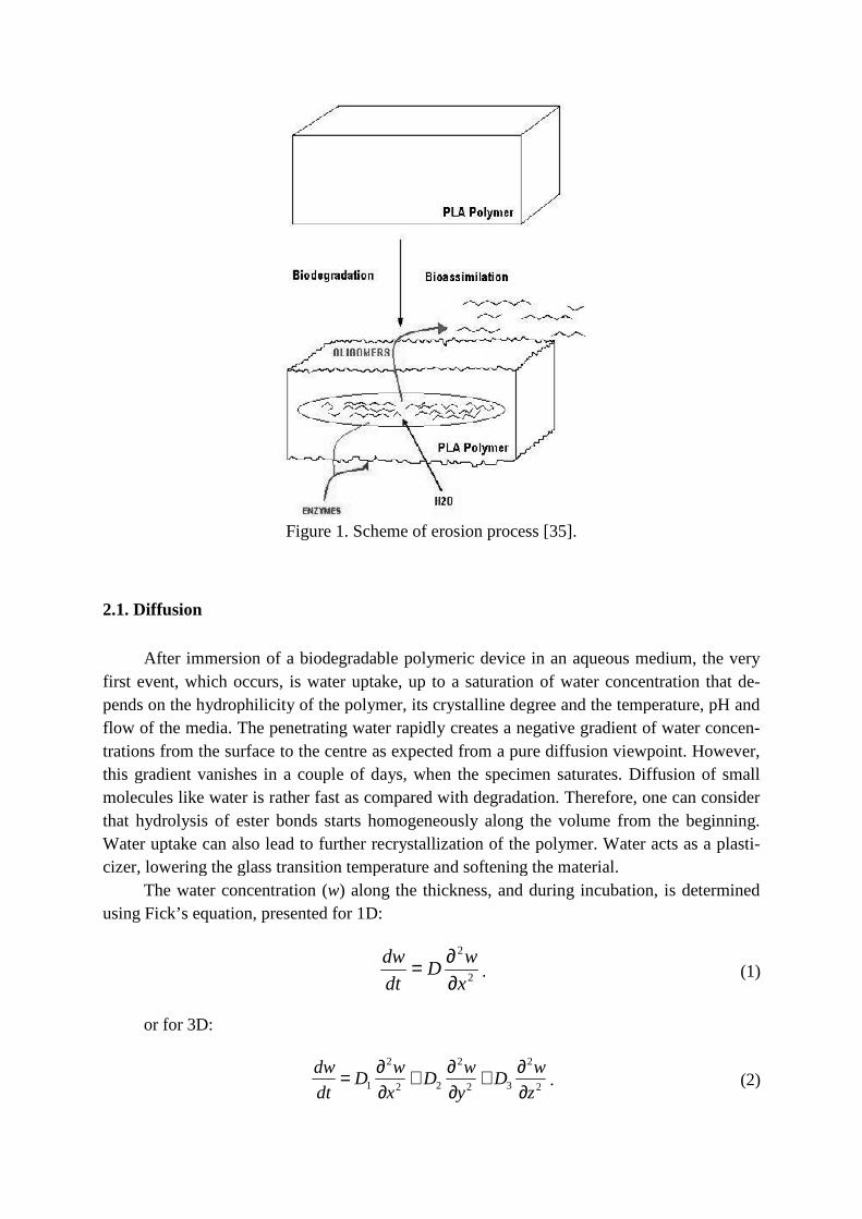
Figure 1.

2.1. Diffusion

After immersion of a biodegradable polymeric device in an aqueous medium, the very first event, which occurs, is water uptake, up to a saturation of water concentration that dpends on the hydrophilicity of the polymer, its crystalline degree and the temperature, pH and flow of the media. The penetrating water rapidly creates a negative gradient of water concetrations from the surface to the centre as expected from a pure diffusion viewpointhis gradient vanishes in a couple of days, when the specimen saturates. Diffusion of small molecules like water is rather fast as compared with degradation. Therefore, one can consider that hydrolysis of ester bonds starts homogeneously along Water uptake can also lead to further recrystallization of the polymer. Water acts as a plastcizer, lowering the glass transition temperature and softening the material.

The water concentration (using Fick’s equation, presented for 1D:

or for 3D:

Figure 1. Scheme of erosion process [35].

After immersion of a biodegradable polymeric device in an aqueous medium, the very is water uptake, up to a saturation of water concentration that d

hydrophilicity of the polymer, its crystalline degree and the temperature, pH and flow of the media. The penetrating water rapidly creates a negative gradient of water concetrations from the surface to the centre as expected from a pure diffusion viewpointhis gradient vanishes in a couple of days, when the specimen saturates. Diffusion of small molecules like water is rather fast as compared with degradation. Therefore, one can consider that hydrolysis of ester bonds starts homogeneously along the volume from the beginning. Water uptake can also lead to further recrystallization of the polymer. Water acts as a plastcizer, lowering the glass transition temperature and softening the material.

The water concentration (w) along the thickness, and during incubation, is determined using Fick’s equation, presented for 1D:

2

2

x

wD

dt

dw

∂∂= .

2

2

32

2

22

2

1 z

wD

y

wD

x

wD

dt

dw

∂∂+

∂∂+

∂∂= .

After immersion of a biodegradable polymeric device in an aqueous medium, the very is water uptake, up to a saturation of water concentration that de-

hydrophilicity of the polymer, its crystalline degree and the temperature, pH and flow of the media. The penetrating water rapidly creates a negative gradient of water concen-trations from the surface to the centre as expected from a pure diffusion viewpoint. However, this gradient vanishes in a couple of days, when the specimen saturates. Diffusion of small molecules like water is rather fast as compared with degradation. Therefore, one can consider

the volume from the beginning. Water uptake can also lead to further recrystallization of the polymer. Water acts as a plasti-

during incubation, is determined

(1)

(2)

The diffusion rate D of the material can be determined by measuring moisture absorp-tion increased weight during incubation. In the case of isotropic polymers, diffusion has no preferential direction, and D1=D2=D3=D.

2.2. Hydrolysis

The macromolecular skeleton of many polymers comprises chemical bonds, which can go through hydrolysis in the presence of water molecules, leading to chain scissions. In the case of aliphatic polyesters, these scissions occur at the ester groups. A general consequence of such process is the lowering of the plastic flow ability of the polymer, causing the change of a ductile, tough behavior into a brittle one. If the behavior was initially brittle, there will be an increase in the brittleness. In Figure 2, it is presented a scheme of the most common hy-drolysis mechanism. Each polymer molecule, with its own carboxylic and alcohol end groups, is broken in two, randomly in the middle at a given ester group. So, the number of carboxylic end groups will increase with degradation time, while the molecules are being split by hy-drolysis.

Figure 2. Acid catalyzed hydrolysis mechanism [38]. Hydrolysis has traditionally been modeled using a first order kinetics equation based on

the kinetic mechanism of hydrolysis, according to the Michaelis–Menten scheme [5]. Accord-ing to Farrar and Gillson [12] the following first-order equation describes the hydrolytic pro-cess relative to the carboxyl end groups (C), ester concentration (E) and water concentration (w):

uCkEwCdt

dC == . (3)

where u is the medium hydrolysis rate of the material , k is the hydrolysis rate constant E and w are constant in the early stages of the reaction. In addition, water is spread out uni-formly in the sample volume (no diffusion control). Using the molecular weight, and since the concentrations of carboxyl end groups are given by C=1/Mn; the equation 3 becomes:

ut

nn eMMt

−=0

. (4)

where Mnt and Mn0, are the number-average molecular weight, at a given time t and ini-tially at t = 0, respectively. This equation leads to a relationship Mn =f(t). However, in the design phase of a biodegradable device, it is important to predict the evolution of mechanical properties like tensile strength, instead of molecular weight. It has been shown by Vieira et al. [38] that the fracture strength follows the same trend as the molecular weight:

ut

t e−= 0σσ . (5)

The hydrolytic damage can be written, as Vieira et al. [38], in the form:

kEwtut eed −− −=−=−= 111

0h σ

σ. (6)

So the hydrolytic damage depends on the hydrolysis kinetic constant, k, the concentra-tions of ester groups, E, the water concentration in the polymer matrix, w, and the degradation time. In this example, of homogeneous degradation with instant diffusion, the degradation rate, u, is constant, and damage only depends on degradation time. Although these considera-tions are valid in the majority of the cases, in some cases the degradation rate cannot be con-sidered constant.

2.3. Surface vs. Bulk erosion

Different types of erosion are illustrated in Figure 3. One is homogeneous or bulk ero-sion without autocatalysis (Figure 3(c)), considered until now, where diffusion is considered to occur instantaneously. Hence, the decrease in molecular weight, the reduction in mechani-cal properties, and the loss of mass occur simultaneously throughout the entire specimen. One other type is heterogeneous or surface erosion (Figure 3(a)), in which hydrolysis occurs in the region near the surface, whereas the bulk material is only slightly or not hydrolyzed at all. As the surface is eroded and removed, the hydrolysis front moves through the material core. In this case, in which diffusion is very slow compared to hydrolysis, one must use equation 1 to calculate water concentration w(t, x) at any instant t through the thickness x, before using equations 4 and 5. Surface eroding polymers have greater ability to achieve zero-order release

kinetics, and are therefore ideal candidates for developing devices able to deliver substances such as drugs, aroma, fertilizesion, since enzymes are unable to diffuse and present a rais

Figure 3. Schematic illustration of three types of erosion phenomenon: (a) surface erosion, (b) bulk erosion with autocatalysis, (c) bul

Surface and bulk erosion are ideal cases to which most polymers cannot be unequiv

cally assigned. It can be definedation rate:

If D is the diffusion coefficient of water in the polymer and can be defined a characteristic time of diffusion,

When τH >> τD, water reaches the core of the material before it reacts, and the degradtion starts homogenously. When never reach the core of the material. The degradation starts heterogeneously through the voume. In these cases, a higher surface to volume ratio induces a faster degradation. Another factor, which complicates the erosion of biodegradablesautocatalytic [28]. For example, a thick plate of PLA erodes faster ththe same polymer [15]. This occurs due to retention ofwithin the material, which are carboxylic acids, causing a local decrease in pH and thereforeaccelerating the degradation [14]as a consequence [15].

kinetics, and are therefore ideal candidates for developing devices able to deliver substances such as drugs, aroma, fertilizers, etc [23]. Also enzymatic erosion fits on this last type of ersion, since enzymes are unable to diffuse and present a raised hydrolysis kinetic constant

Schematic illustration of three types of erosion phenomenon: erosion, (b) bulk erosion with autocatalysis, (c) bulk erosion without autocatalysis

[38].

Surface and bulk erosion are ideal cases to which most polymers cannot be unequivdefined the characteristic time of hydrolysis, as the i

mH ukEw

11 ==τ .

is the diffusion coefficient of water in the polymer and L is the sample thickness, a characteristic time of diffusion, τD:

D

LD

2

=τ .

reaches the core of the material before it reacts, and the degradtion starts homogenously. When τH << τD, water reacts totally in the superficial layer and will never reach the core of the material. The degradation starts heterogeneously through the vo

e. In these cases, a higher surface to volume ratio induces a faster degradation. Another complicates the erosion of biodegradables, consists on the hydrolysis reaction is

For example, a thick plate of PLA erodes faster than a thinner one made of . This occurs due to retention of the oligomeric hydrolysis products

within the material, which are carboxylic acids, causing a local decrease in pH and therefore[14]. As can be seen in Figure 3(b), hollow structures are formed

kinetics, and are therefore ideal candidates for developing devices able to deliver substances . Also enzymatic erosion fits on this last type of ero-

ed hydrolysis kinetic constant k.

Schematic illustration of three types of erosion phenomenon: k erosion without autocatalysis

Surface and bulk erosion are ideal cases to which most polymers cannot be unequivo-the characteristic time of hydrolysis, as the inverse of degra-

(7)

is the sample thickness, it

(8)

reaches the core of the material before it reacts, and the degrada-, water reacts totally in the superficial layer and will

never reach the core of the material. The degradation starts heterogeneously through the vol-e. In these cases, a higher surface to volume ratio induces a faster degradation. Another

consists on the hydrolysis reaction is an a thinner one made of

the oligomeric hydrolysis products within the material, which are carboxylic acids, causing a local decrease in pH and therefore,

b), hollow structures are formed

3. CONSTITUTIVE MODELS FOR BIODEGRADABLE MATERIALS

A constitutive model for a mechanical analysis is a relationship between the response of a body (for example, strain) and the stress due to the forces acting on this body. A wide variety of material behaviors are described with a few different classes of constitutive equa-tions. Due to the nonlinear nature of the stress vs. strain plot, the classical linear elastic model is clearly not valid for large deformations. Hence, given the nature of biodegradable plastic, classical models such as the neo-Hookean and Mooney-Rivlin models for incompressible hyperelastic materials may be used to describe its mechanical behavior until rupture. For these materials, stiffness depends on the fiber stretch. Mechanical properties of elastomeric materi-als are usually represented in terms of a strain energy density function W, which is a scalar function of the deformation gradient. W can also be represented as a function of the right Cauchy–Green deformation tensor invariants. In general, the strain energy density for an iso-tropic, incompressible, hyperelastic material is determined by two invariants. The first and second invariants in uniaxial tension are given by:

λλ 22 +=CI . (9)

λλ

21

2+=CII . (10)

where λ is the axial stretch (λ=1+ε), that satisfies λ≥1. The neo-Hookean incompressi-ble hyperelastic solid is given by stored energy function:

)3(2

1 −= CIWµ

. (11)

where µ1 > 0 is the material property, usually designed as the shear modulus. An ex-tension of this model is the Mooney-Rivlin incompressible hyperelastic solid, which stored energy function has the form equal to:

)3(2

)3(2

21 −+−= CC IIIWµµ

. (12)

with two material properties µ1 and µ2. Higher order stored energy functions may be considered to describe the experimental data, such as a reduced 2nd order stored energy func-tion, which includes a mixed term with both invariants of the right Cauchy–Green stretch ten-sor and an extra material constant µ3, which stored energy function has the form equal to:

)3)(3(6

)3(2

)3(2

321 −−+−+−= CCCC IIIIIIWµµµ

. (13)

The axial nominal stress for the three models, neo-Hookean (σNH), Mooney-Rivlin

(σMR) and reduced second order (σ2nd red), will be given by:

1 2

1( )NHσ µ λ

λ= − . (14)

)1

1()1

(3221 λ

µλ

λµσ −+−=MR. (15)

)1

()1

1)(()1

)((4

23332231

2

λλµ

λµµ

λλµµσ −+−−+−−=rednd

. (16)

According to Soares et al. [29], the model constitutive material parameters depend on degradation time. The material parameters are considered to be material functions of degrada-tion damage instead of material constants. Later, Vieira et al. [38] determined that only the first material parameter µ1, vary linearly with hydrolytic damage (as defined in Eq. 6). In this work, a blend of PLA-PCL (90:10) was used. From Fig. 4, one can see that the hyperelastic material models fit well the measured storage energy, for all the degradation steps up to 8 weeks.

Figure 4. Storage energy vs. axial stretch for 0, 2, 4 and 8 weeks of degradation [38].

The experimental data of storage energy was calculated by measuring the area (i.e., by taking the integral) underneath the stress-strain curve, from zero until a certain level of stretch. The neo-Hookean model was the less precise. However it respects the 2nd law of thermodynamics where every material parameters µi must have a positive value. The material parameters were calculated by inverse parameterization of the models with the experimental data, and are listed in Table 2.

Table 2. Evolution of the model material parameters during degradation [38].

Material Models weeks d µ1 µ2 µ3

Neo-Hookean

0 0.00 450

- - 2 0.18 410 4 0.33 364 8 0.55 364 16 0.80 630

Mooney-Rivlin

0 0.00 80

500 - 2 0.18 50 4 0.33 5 8 0.55 -30 16 0.80 150

2nd reduced order

0 0.00 155

400 -1 2 0.18 120 4 0.33 75 8 0.55 50 16 0.80 250

From Figure 5, one can see that the hyper elastic material models allowed a reasonable

approximation of the tensile test results. The presented method, that consists on changing the first material parameter with hydrolytic damage, µ1(d) , according to the linear regression (see Figure 6), enables to describe the mechanical behavior evolution by using equations 14, 15 or 16, while the limit stress is defined by equation 5.

These constitutive models can be implemented in commercial finite element software packages like ABAQUS, by changing the material parameter as function of hydrolytic dam-age or degradation time, and associated to the failure criterion. Besides, this implementation can be performed through a User Material (UMAT) subroutine.

Figure 5. Axial nominal stress vs. strain for 0, 2, 4 and 8 weeks of degradation (experimental

data and material models) [38].

Figure 6. Evolution of the material parameter, µ1, of the models during degradation [38].

4. IMPLEMENTATION AND APPLICATION OF THIS NEW APPROACH FOR NUMERICAL ANALYSIS OF BIODEGRADABLE PLASTIC STRUCTURES

In this section, an example of the new approach for predicting the life-cycle of a hy-drolytic degradable device, and its implementation in ABAQUS standard is shown, using the Neo-Hookean material model. This is used to simulate PLA-PCL behavior for fiber geometry. As commented earlier, this implementation was carried out using a subroutine UMAT as well as the PYTHON programming language. Although Neo-Hookean model was less accurate than the other models, it is not so complicate to implement, since it uses only one material parameter µ1. Furthermore, it avoids the violation of the 2nd Law of Thermodynamics, which happens for the other models when negative values for the material parameters (µ2 and µ3) take place. For this 3D case, the first and second invariants of deviator part of the left Cauchy-Green deformation tensor are given by:

r(B)t=I B . (17)

1/222

B ]trB -1/2[(trB)=II . (18)

where B is the deviator stretch tensor (B=FFT). The Neo-Hookean compressible hyper elastic model is given by stored energy function of the form equal to:

2

B1 1)-G(J+3)-/2)(I(µ=W . (19)

where G is a material constant that depends on the compressibility (G=0 for in-compressible materials). J is the determinant of the deformation gradient (J=1 for incompress-ible materials):

X)x/det(=J ∂∂ . (20)

where x is the current 3D position of a material point and X is the reference position of the same point. Then:

X)x/(J=F -1/3 ∂∂ . (21)

is the deformation gradient with volume change eliminated. The Cauchy stress tensor for the Neo-Hookean model used in this example is given by:

1)I-2G(J+dev(B) /J) µ(=T 1 . (22)

where I is the 2nd order identity tensor. The first material parameter is calculated as function of the hydrolytic damage, µ1(dh),

according to a linear regression shown in Figure 6. In this example, a 3D model of a fiber was developed by means of a script in PYTHON language, using solid and axisymmetric ele-ments, with parabolic interpolation functions, as well as with reduced and/or hybrid integra-

tion. This script is run by ABAQUS andter data (Figure 7). The hydrolysis rate of the material (degraded material (σ0) are initially set in the command lines. The material was considered nearly incompressible (G = 10cording to equation 6, and the material strength (radation time (t). The script also calculates the material parameter (C10of the hydrolytic damage C10(and G) are considered input data for the UMAT subroutine, as shown

Figure 7. Flow of operations done by ABAQUS/PYTHON and the UMAT subroutine

Based on the geometry, the loadings and boundary conditions, ABAQUS calculates

the variables, which correspond to the deformation gradient lates the Jacobian (J) and the distortion tensor (tively, for each integration point of the then calculated before the calculation of stress Cauchy tensor The implemented UMAT compares the principal stresses each integration point, acting as a failure criterion. Whenever these are greater than the strength, for a certain increment, the subroutine sets them to zero in the finite element anlyzed. Finally, the UMAT builtscrement into the OBD (Output Base Data) file of ABAQUS. The flow chart of calculi opertions is represented in Figure 7

Figure 8(a) shows the mesh of the finite element model and boundary condiplied, as well as a numerical result for maximum principal stress. The CAX8H (8quadratic axisymmetric quadrilateral, hybrid, linear pressure element) and C3D20RH (20node quadratic brick, hybrid, linear pressurewith similar results. Although the first element type is simpler and faster to calculate, it ca

tion. This script is run by ABAQUS and the degradation time is required as an input param). The hydrolysis rate of the material (u) and the strength of the non

) are initially set in the command lines. The material was considered 10-3). Then the script calculates the hydrolytic damage (

, and the material strength (σt) according to equation ). The script also calculates the material parameter (C10 =

of the hydrolytic damage C10(dh). The material strength (σt) and the material parameters (C10 ) are considered input data for the UMAT subroutine, as shown by Figure

Flow of operations done by ABAQUS/PYTHON and the UMAT subroutine

Based on the geometry, the loadings and boundary conditions, ABAQUS calculates correspond to the deformation gradient (∂x/∂X). Then, the UMAT calc) and the distortion tensor (F), according to Equation

tively, for each integration point of the finite elemen model. The deviator stretch tensor B is then calculated before the calculation of stress Cauchy tensor T, according to Equation The implemented UMAT compares the principal stresses (σ1, σ2 and σ3) to the strength (each integration point, acting as a failure criterion. Whenever these are greater than the strength, for a certain increment, the subroutine sets them to zero in the finite element an

builts the constitutive matrix and calculates the result for each icrement into the OBD (Output Base Data) file of ABAQUS. The flow chart of calculi oper

7. a) shows the mesh of the finite element model and boundary condi

plied, as well as a numerical result for maximum principal stress. The CAX8H (8quadratic axisymmetric quadrilateral, hybrid, linear pressure element) and C3D20RH (20node quadratic brick, hybrid, linear pressure, reduced integration) elemenwith similar results. Although the first element type is simpler and faster to calculate, it ca

the degradation time is required as an input parame-) and the strength of the non-

) are initially set in the command lines. The material was considered ). Then the script calculates the hydrolytic damage (dh) ac-

quation 5, for a given deg-= µ1/2) as a function

) and the material parameters (C10 Figure 7.

Flow of operations done by ABAQUS/PYTHON and the UMAT subroutine [36].

Based on the geometry, the loadings and boundary conditions, ABAQUS calculates ). Then, the UMAT calcu-

), according to Equation 20 and 21 respec-model. The deviator stretch tensor B is

, according to Equation 22. ) to the strength (σt) for

each integration point, acting as a failure criterion. Whenever these are greater than the strength, for a certain increment, the subroutine sets them to zero in the finite element ana-

the constitutive matrix and calculates the result for each in-crement into the OBD (Output Base Data) file of ABAQUS. The flow chart of calculi opera-

a) shows the mesh of the finite element model and boundary conditions ap-plied, as well as a numerical result for maximum principal stress. The CAX8H (8-node bi-quadratic axisymmetric quadrilateral, hybrid, linear pressure element) and C3D20RH (20-

tion) element types were used, with similar results. Although the first element type is simpler and faster to calculate, it can-

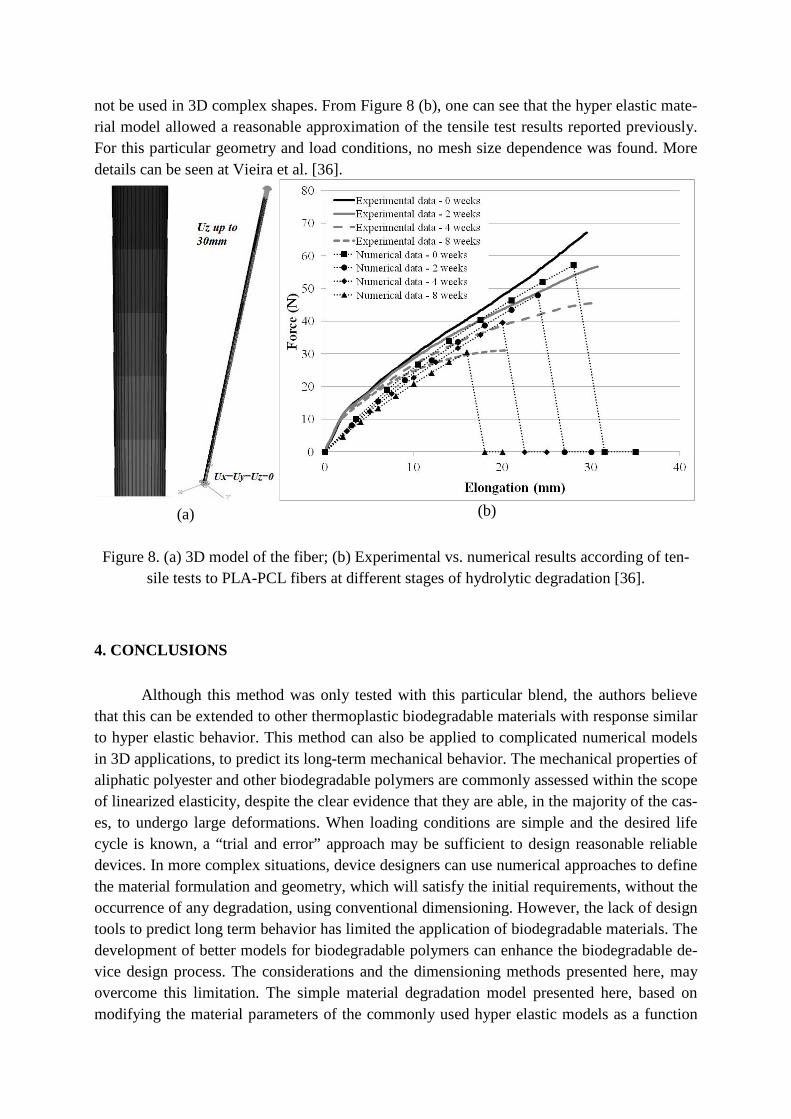
not be used in 3D complex shapes. From Figure 8 (b), one can see that the hyper elastic mate-rial model allowed a reasonable approximation of the tensile test results reported previously. For this particular geometry and load conditions, no mesh size dependence was found. More details can be seen at Vieira et al. [36].

(a) (b)

Figure 8. (a) 3D model of the fiber; (b) Experimental vs. numerical results according of ten-

sile tests to PLA-PCL fibers at different stages of hydrolytic degradation [36].

4. CONCLUSIONS

Although this method was only tested with this particular blend, the authors believe that this can be extended to other thermoplastic biodegradable materials with response similar to hyper elastic behavior. This method can also be applied to complicated numerical models in 3D applications, to predict its long-term mechanical behavior. The mechanical properties of aliphatic polyester and other biodegradable polymers are commonly assessed within the scope of linearized elasticity, despite the clear evidence that they are able, in the majority of the cas-es, to undergo large deformations. When loading conditions are simple and the desired life cycle is known, a “trial and error” approach may be sufficient to design reasonable reliable devices. In more complex situations, device designers can use numerical approaches to define the material formulation and geometry, which will satisfy the initial requirements, without the occurrence of any degradation, using conventional dimensioning. However, the lack of design tools to predict long term behavior has limited the application of biodegradable materials. The development of better models for biodegradable polymers can enhance the biodegradable de-vice design process. The considerations and the dimensioning methods presented here, may overcome this limitation. The simple material degradation model presented here, based on modifying the material parameters of the commonly used hyper elastic models as a function

of degradation time, can perfomr a reasonable prediction of the life time of complex biode-gradable devices.

Acknowledgements

Volnei Tita would like to thank Research Foundation of State of Sao Paulo (process number: 09/00544-5). The authors would like to highlight that this work was also partially supported by the Program USP/UP, which is a scientific cooperation agreement established between the University of Porto (Portugal) and the University of São Paulo (Brazil).

5. REFERENCES

[1] Agarwal M., Koelling K. W., Chalmers J. J., “Characterization of the Degradation of Po-lylactic Acid Polymer in a Solid Substrate Environment”. Biotechnol. Prog. 14, 517-526, 1998.

[2] Ashammakhi N., Mäkelä E. A., Vihtonen K., Rokkanen P., Kuisma H., Tormala P., “Strength retention of self-reinforced polyglycolide membrane: an experimental study”. Biomaterials. 16, 135-138, 1995.

[3] Aslan S., Calandrelli L., Laurienzo P., Malinconico M., Migliares C., “Poly(d,l-lactic acid)/poly(caprolactone) blend membranes: preparation and morphological characteriza-tion”. J. Mater. Sci. 35, 1615–1622, 2000.

[4] Auras R., Harte B., Selke S., “An Overview of Polylactides as Packaging Materials”. Ma-cromol. Biosci. 4, 835–864, 2004.

[5] Bellenger V., Ganem M., Mortaigne B., Verdu J., “Lifetime prediction in the hydrolytic ageing of polyesters”. Polym. Degrad. Stab. 49, 91–97, 1995.

[6] Bikiaris D. N., Papageorgiou G. Z., Achilias D. S., “Synthesis and comparative biodegra-dability studies of three poly(alkylene succinate)s”. Polym. Degrad. Stab. 91, 31- 43, 2006.

[7] Chen C-C., Chueh J.-Y., Tseng H., Huang H.-M., Lee S.-Y., “Preparation and characteri-zation of biodegradable PLA polymeric blends”. Biomaterials. 24, 1167–1173, 2003.

[8] Chen G.-Q., Wu Q., “Review:The application of polyhydroxyalkanoates as tissue enginee-ring materials”. Biomaterials. 26, 6565–6578, 2005.

[9] Cohn D., Hotovely-Salomon A., “Biodegradable multiblock PEO/PLA thermoplastic elas-tomers: molecular design and properties”. Polymer. 46, 2068–2075, 2005.

[10] Colombo A., Karvouni E., “Biodegradable stents: fulfilling the mission and stepping away”. Circulation. 102, 371-373, 2000.

[11] Fan L., Nan C.-W., Li M., “Thermal, electrical and mechanical properties of (PEO)16LiClO4 electrolytes with modified montmorillonites”. Chem. Phys. Lett. 369, 698–702, 2003.

[12] Farrar D. F., Gillson R. K., “Hydrolytic degradation of polyglyconate B: the rela-tionship between degradation time, strength and molecular weight”. Biomaterials. 23, 3905–3912, 2002.

[13] Ferretti A, Carreau P. J., Gerard P., “Rheological and Mechanical Properties of PEO/Block Copolymer Blends”. Polym. Eng. Sci. 45, 1385–1394, 2005.

[14] Göpferich A., “Mechanism of polymer degradation and erosion”. Biomaterials. 23, 103–114, 1996.

[15] Grizzi I., Garreau H., Li S., Vert M., “Hydrolytic degradation of devices based on po-ly[DL-lactic acid) size-dependence”. Biomaterials. 16, 305-311, 1995.

[16] Herzog K., Muller R.-J., Deckwer W.-D., “Mechanism and kinetics of the enzymatic hydrolysis of polyester nanoparticles by lipases”. Polym. Degrad. Stab. 91, 2486–2498, 2006.

[17] Hong J.-T., Cho N.-S., Yoon H.-S., Kim T.-H., Koh M.-S., Kim W.-G., “Biodegradable Studies of Poly(trimethylenecarbonate-e-caprolactone)-block-poly(p-dioxanone), Po-ly(dioxanone), and Poly(glycolide-e-caprolactone) (Monocryl) Monofilaments”. J. Appl. Polym. Sci. 102, 737–743, 2006.

[18] Langer L., “Drug delivery and targeting.”, Nature. 392, 5-10, 1998. [19] Laufman H., Rubel T., “Synthetic absordable sutures”. Surg. Gynecol. Obstet. 145,

597–608, 1977. [20] Levenberg S., Langer R., “Advances in tissue engineering”. Ed. Schatten, G.P., “Cur-

rent topics in developemental biology“. Elsevier Academic, San Diego, 113, 2004. [21] Mohantya A. K., Misra M., Hinrichsen G., “Biofibres, biodegradable polymers and bio-

composites: An overview”. Macromol. Mater. Eng. 276-277, 1–24, 2000. [22] Nagarajan S., Sudhakar S., Srinivasan K. S. V. “Poly(ethylene glycol) block copoly-

mers by redox process: kinetics, synthesis and characterization”. Pure. & Appl. Chem. 70, 1245-1248, 1998.

[23] Nair L. S., Laurencin C. T., “Biodegradable polymers as biomaterials”, Prog. Polym. Sci. 32, 762–798, 2007.

[24] Navarro M., Ginebra M. P., Planell J. A., Barrias C. C., Barbosa M. A., “In vitro degra-dation behavior of a novel bioresorbable composite material based on PLA and a soluble CaP glass”. Acta Biomaterialia. 1, 411–419, 2005.

[25] Nikolic M. S., Poleti D., Djonlagic J., “Synthesis and characterization of biodegradable poly(butylenes succinate-co-butylene fumarate)s”. Eur. Polym. J. 39, 2183-2192, 2003.

[26] Oksmana K., Skrifvars M., Selinc J.-F., “Natural fibres as reinforcement in polylactic acid (PLA) composites”. Comp. Sci. Tech. 63, 1317–1324, 2003.

[27] Pietrzak W. S., Sarver D. R, Verstynen M. L., “Bioabsorbable polymer science for the practicing surgeon.”, J. Craniofac. Surg. 8, 87-91, 1997.

[28] Siparsky G.L., Voorhees K.J., Miao F., “Hydrolysis of polylactic acid (PLA) and poly-caprolactone (PCL) in aqueous acetonitrile solutions: autocatalysis.” J. Polym. Environ. 6, 31–41, 1998.

[29] Soares J. S., Rajagopal K. R., Moore J. E., “Deformation-induced hydrolysis of a de-gradable polymeric cylindrical annulus”. Biomech. Model. Mechaobiol. 9, 177-186, 2010.

[30] Södergard A., Stolt M., “Properties of lactic acid based polymers and their correlation with composition”. Prog. Polym. Sci. 27, 1123-1163, 2002.

[31] Tamela T. L., Talja M., “Biodegradable urethral stents”. B.J.U. Int. 92, 843-850, 2003. [32] Todo M., Park S.-D., Takayama T., Arakawa K., “Fracture micromechanisms of bioab-

sorbable PLLA/PCL polymer blends”. Eng. Fract. Mech. 74, 1872–1883, 2007. [33] Tsuji H., Ikada Y., “Blends of Aliphatic Polyesters. I. Physical Properties and Morpho-

logies of Solution-Cast Blends f rorn Poly(Di-lactide) and Poly(e-caprolactone)”. J. Appl. Polym. Sci. 60, 2367-2375, 1996.

[34] Van de Velde K., Kiekens P., “Biopolymers: overview of several properties and conse-

quences on their applications”. Polymer. Testing. 21, 433–442, 2002. [35] Vieira A. C., “Degradation Parameters and Mechanical Properties Evolution”. Ed Bran-

don M. Johnson and Zachary E. Berkel, “Biodegradable Materials: Production, Properties and Applications”. ISBN: 978-1-61122-804-5, Nova Publisher, 2011.

[36] Vieira A. C., Marques A. T., Guedes R. M., Tita V., «Material model proposal for bio-degrada-ble materials». Procedia. Engineering. 10, 1597–1602, 2011.

[37] Vieira A.C., Guedes R.M., Marques A.T., “Development of ligament tissue biodegra-dable devices: A review”. J. Biomech. 42, 2421–2430, 2009.

[38] Vieira A.C., Vieira J.C., Ferra J., Magalhães F.D., Guedes R.M., Marques A.T., “Me-chanical study of PLA–PCL fibers during in vitro degradation”. J. Mech. Behav. Biomed. 4, 451-60, 2011.

[39] Yew G. H., Yuzof A.M., Ishak Z.A., Ishiaku U.S., “Water absorption and enzymatic degradation of poly(lactic acid)/rice starch composites”. Polym. Degrad. Stab. 90, 488-500, 2005.

[40] Zhang X., Hua H., Shen X., Yang Q., “In vitro degradation and biocompatibility of po-ly(L-lactic acid)/chitosan fiber composites”. Polymer. 48, 1005-1011, 2007.

[41] Zilberman M., “Novel composite Wber structures to provide drug/protein delivery for medical implants and tissue regeneration”. Acta. Biomaterialia. 3, 51–57, 2007.

[42] Zuideveld M., Gottschalk C., Kropfinger H., Thomann R., Rusu M., Frey H., “Miscibi-lity and properties of linear poly(L-lactide)/branched poly(L-lactide) copolyester blends”. Polymer. 47, 3740–3746, 2006.