1

Material Flows and Environmental Impacts of Manufacturing Systems via Aggregated

Input-Output Models

H. Xue*, V. Kumar, and J. W. Sutherland

Department of Mechanical Engineering and Engineering Mechanics Michigan Technological University

1400 Townsend Drive Houghton, Michigan 49931, USA

ABSTRACT

Manufacturing processes may be viewed as operational units in the overall manufacturing/production system.

Changes in technology, production patterns, and process settings are typically made at the process (unit) level. Very

often, environmental problems are apparent when the manufacturing/production system is viewed as a whole (many

units joined together). However, with the units aggregated to form a system, it is often difficult to identify the source

of an environmental problem or judge the singular effect of changes to a process unit; the changes become lost in the

complexity of the system as a whole. Recent efforts have employed input-output modeling to describe the flow of

materials and the environmental consequences associated with manufacturing processes. A method is introduced for

aggregating process-level material input-output models to form a combined material input-output model for a

manufacturing system. This resulting model serves as a bridge between unit-level changes and broader system

behaviors. The model form permits identification of opportunities for reducing environmental impacts at the process

level (e.g., reduction of emissions, waste generation, and material use) and driving the system toward zero emissions

based on an examination of the aggregated manufacturing system level model. Case studies are used to illustrate the

application of the aggregated material input-output model to minimizing waste and resource consumption.

Keywords: Input-Output, Material Flows, Environmental Impact, Model Aggregation, Zero Emission

* Corresponding author. Fax: 313-594-4521. E-mail address: hxue1@ford.com.

2

NOTATION

aij technical coefficients related to original inputs to the process

A technical coefficient matrix related to original inputs in the process, or the aggregated technical coefficient matrix

in a manufacturing system

bij technical coefficients related to new generated substances in the process

B technical coefficient matrix related to new generated substances in the process, or the aggregated technical

coefficient matrix in a manufacturing system

wij material flow from material i to new substance j

xi amount of input to the process

Xi the total output, or production, of sector i in an economic system

X vector of process inputs

yi output from the process in new substance forms

Yi the total final demand for i’s product in an economic system

Y vector of process outputs

Y estimate of Y

zij flow of input from sector i to sector j in an economic system, or the material flow from material i to material j in

physical unit

α weighting factor

β weighting factor

1. Introduction

Manufacturing processes in various industries, especially the chemical, automotive, electronics, and pulp and paper

industries, produce adverse environmental impacts such as waste generation, energy consumption, and the release of

hazardous substances. Process-centered efforts have been demonstrated to be an extremely effective means for

achieving the goal of reducing the environmental impact [1]. If manufacturing process innovations are employed to

achieve improved environmental performance, competitiveness will be indirectly benefited because of reduced costs

associated with controlling and containing environmental impacts. Competitiveness will be directly benefited because

3

the innovations are likely to produce lower costs, higher productivity, and better quality products. Of course, the

ultimate class of innovations are those that produce zero emissions.

One way of characterizing a manufacturing process is by materials flow analysis. Such an analysis can convert process

inputs into intermediate products or final products, and can consider a range of mechanisms, e.g., mechanical and

chemical. For manufacturing processes, the principal environmental impacts are associated with the process outputs,

which may take the form of solid, liquid, and gaseous emissions. Materials flow analysis identifies the amounts of

inputs and outputs associated with a process and then relates the inputs and outputs to provide a mathematical model

that can be used to explore opportunities for reduced environmental impact. To establish an input-output relation, it is

preferable to formulate a mathematical description based on physical, chemical, and other natural laws [2, 3, 4].

Unfortunately, it is often the case that there is insufficient knowledge or process information to develop a mechanistic

model of a manufacturing process. However, in practice, such a mechanistic understanding of the process may not be

needed; this is especially true during the beginning stages of environmental process improvement, when a simple,

tractable model may be sufficient to identify opportunities for reduced environmental impact. A matrix-based

input-output model represents such a model and is the focus of the effort described in this paper.

Input-output analysis has traditionally been used to analyze economic activities [5], and it has been extended to

address environmental analysis at the national, industry, and product levels [6, 7, 8, 9]. These analyses have provided

insight into the workings of environmental policy and the manifestation of pollution at various levels. For example, in

France the emission of SO2 and NOx was studied by constructing an input-output model to identify the main pollution

sources and to explore the possibilities for different abatement strategies [6]. A number of the complex relations

between energy, environment, and economic welfare were also investigated via a 10-sector input-output model of the

UK [7]. The model was used to simulate the effects of a variety of policies and scenarios through changes in the

demand levels and technical coefficients. In addition, input-output modeling has been used to characterize the

environmental impacts of manufacturing processes [10].

In this paper, we develop environmental input-output models at different spatial scales for such entities as

manufacturing systems, manufacturing plants, and a company. For environmental input-output models developed at

4

large spatial scales, e.g, at national or industry-wide levels, these models are highly aggregated and lack spatial

resolution, and cannot be decomposed or disaggregated to acquire information about the manufacturing systems,

manufacturing plants, and companies. Thus, there is a gap between national and process-level environmental

input-output models. To bridge this gap one needs to think in terms of aggregating process-level models to obtain a

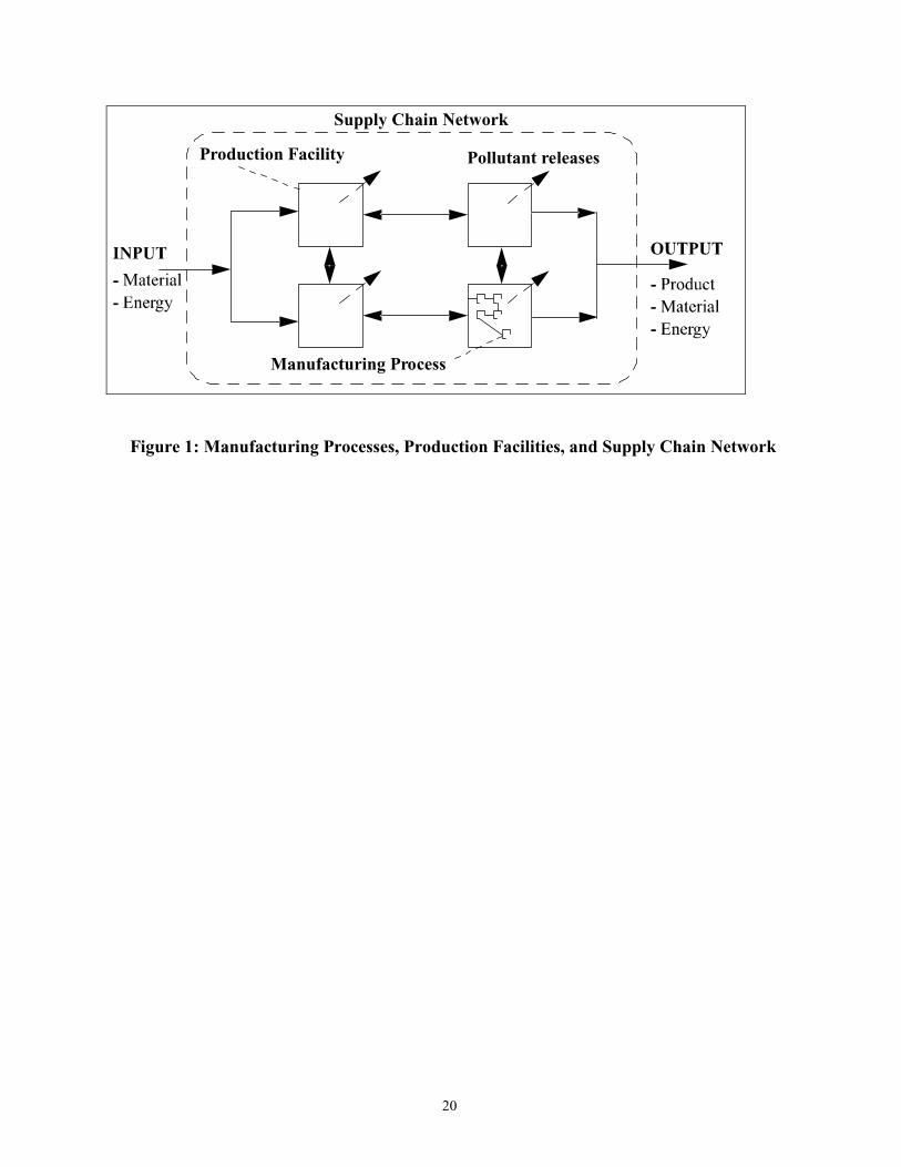
larger scale system-level material input-output model. As shown in Figure 1, manufacturing systems and supply

chains associated with contemporary industrial activities are very complex. Manufacturing unit operations interact

with one another to form manufacturing systems, which in turn interact to form a supply chain. For each

manufacturing process, it is possible to create a material input-output model. These process-level input-output models

may then be aggregated to form a material input-output model for the collection of processes that form the

manufacturing system or even further aggregated to establish a model for the complete supply chain.

Commonly, aggregation within input-output approaches is achieved by consolidating similar economic groups into a

sector. Such an aggregation requires a homogeneous input structure. Several efforts have been made to measure the

effects of aggregation of sectors in input-output models [11, 12, 13, 14, 15, 16]. This paper introduces a method for

aggregating process-level material input-output models to form a combined material input-output model for a

manufacturing system. The model form permits identification of opportunities for reducing environmental impacts at

the process level (e.g., reduction of emissions, waste generation, and material use) based on examination of the

aggregated manufacturing system level model. A case study is used to illustrate the application of the aggregated

material input-output model to minimizing waste and resource consumption and provide guidance on how to drive

processes toward zero emission.

2. Material Input-Output Models for Manufacturing Processes

The economic input-output model popularized by Leontief [5], can be viewed as a simple multi-input multi-output

model. Traditionally, the model has been employed to relate the economic (product) flows from producer sectors to

the consumer sectors. An input-output model is constructed from observed data for a particular economic area such as

a nation, a region, or a state. Its basic notation and fundamental relationships are given by

5

nnnnjnnn

iinijiii

nj

nj

YzzzzX

YzzzzX

YzzzzX

YzzzzX

++++++=

++++++=

++++++=

++++++=

LL

L

LL

L

LL

LL

21

21

22222212

11112111

(1)

where Xi is the total output, or production, of sector i, zij is the flow of input from sector i to sector j, and Yi is the total

final demand for sector i’s product. Equation (1) implies that the products created in sector i are consumed by either

itself or other industrial sectors and that the final demands, along with the amount of production in an underlying

economic system, maintain a balance. By defining a technical coefficientj

ijij X

za = , Equation (1) can be rewritten as:

nnnnnn

nn

nn

YXaXaXa

YXaXaXa

YXaXaXa

=−+−−−

=−−−+−=−−−−

)1(

)1(

)1(

2211

22222121

11212111

L

L

L

L

In matrix form, the above equation becomes

YXA =− )(I (2)

or

YAX 1)( −−= I (3)

where A is called the technical coefficient matrix, I is the n by n identity matrix, and 1)( −− AI is referred to as the

Leontief inverse, if it exists. Therefore, the input-output model represents the dependent relationship between inputs

and outputs within an economic system and is widely used in economics. It should be noted that the input-output

model is based on two fundamental assumptions: the multi-input multi-output relation is linear, and the technical

coefficient is fixed during the underlying time period for which data is available.

When the input-output analysis is used in assessing the environmental impact of manufacturing processes, the

traditional input-output analysis needs to be modified. This is because manufacturing processes have significantly

different characteristics from economic systems. With a traditional input-output model, the number of inputs is equal

6

to the number of outputs. However, when applying input-output modeling to a manufacturing process, the number of

process inputs is not necessarily equal to the number of process outputs. For instance, some inputs are converted into

different substance forms by the process, and other inputs maintain their original form. A second reason for

modification is that the units used in a process input-output model are not monetary units but mass units associated

with the material mass flows of interest. In addition to these reasons, there are no explicit final demands. Consequently,

the structure of the input-output analysis needs to be modified in order to meet the requirements of environmental

impact analysis of manufacturing processes.

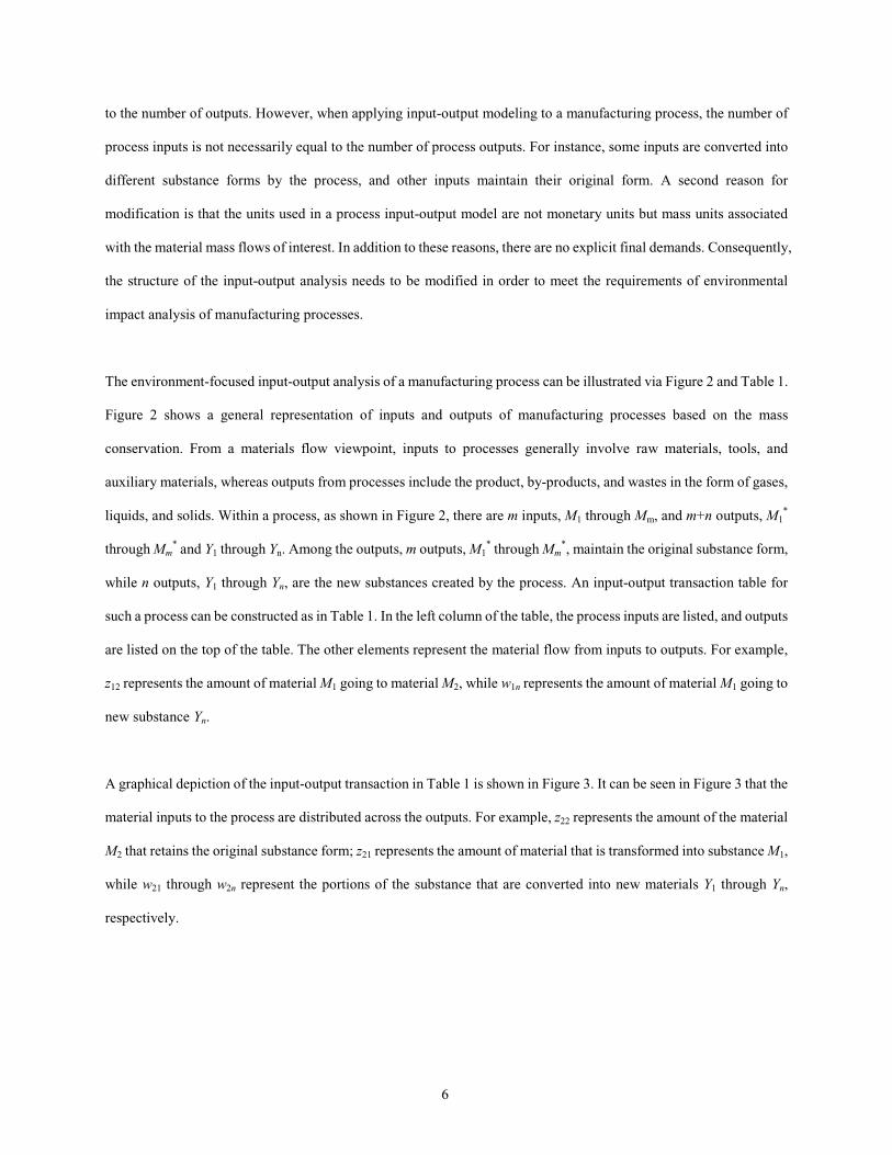
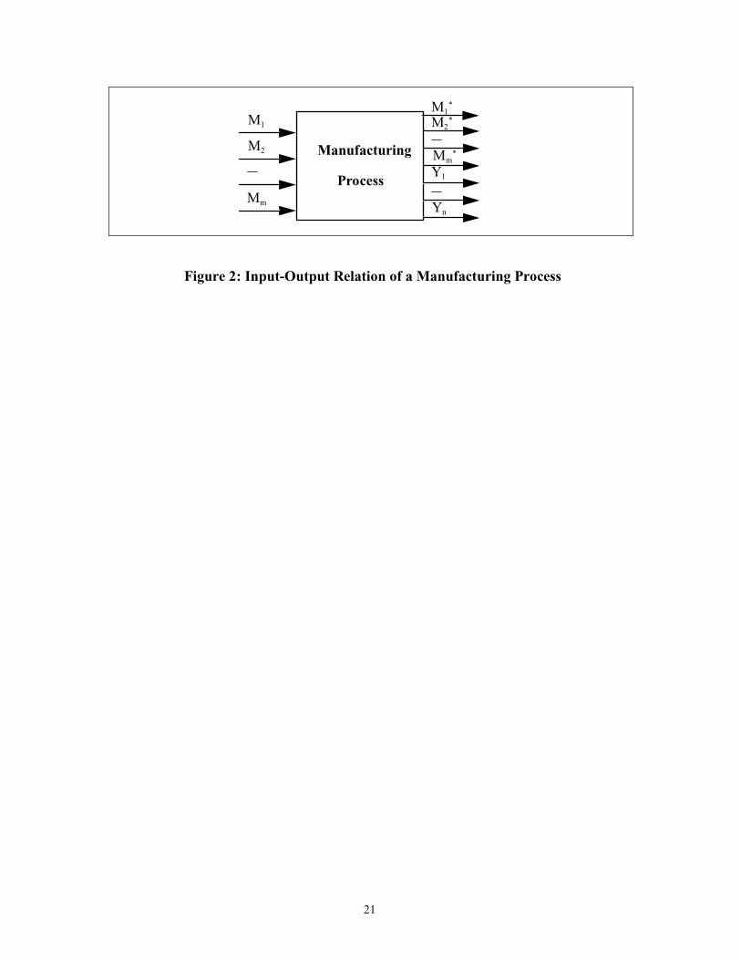
The environment-focused input-output analysis of a manufacturing process can be illustrated via Figure 2 and Table 1.

Figure 2 shows a general representation of inputs and outputs of manufacturing processes based on the mass

conservation. From a materials flow viewpoint, inputs to processes generally involve raw materials, tools, and

auxiliary materials, whereas outputs from processes include the product, by-products, and wastes in the form of gases,

liquids, and solids. Within a process, as shown in Figure 2, there are m inputs, M1 through Mm, and m+n outputs, M1*

through Mm* and Y1 through Yn. Among the outputs, m outputs, M1

* through Mm*, maintain the original substance form,

while n outputs, Y1 through Yn, are the new substances created by the process. An input-output transaction table for

such a process can be constructed as in Table 1. In the left column of the table, the process inputs are listed, and outputs

are listed on the top of the table. The other elements represent the material flow from inputs to outputs. For example,

z12 represents the amount of material M1 going to material M2, while w1n represents the amount of material M1 going to

new substance Yn.

A graphical depiction of the input-output transaction in Table 1 is shown in Figure 3. It can be seen in Figure 3 that the

material inputs to the process are distributed across the outputs. For example, z22 represents the amount of the material

M2 that retains the original substance form; z21 represents the amount of material that is transformed into substance M1,

while w21 through w2n represent the portions of the substance that are converted into new materials Y1 through Yn,

respectively.

7

The development of a mathematical model that relates the inputs and outputs begins by assuming that there is a linear

relationship between each output and its corresponding inputs. Based on this assumption, the following relationship

holds for each input i based on the principle of conservation of matter:

ninjijimimjijii

inijiimijiii

ybybybxaxaxaxa

wwwzzzzx

++++++++++=

++++++++++=

LLLL

LLLL

112211

121 (4)

where xi (i =1, ..., m) is the input amount, yi (i =1, ..., n) is the output from the process in new substance forms, zij is the

material flow from material i to material j, and wij is the material flow from material i to new substance j. All xi, yi, zij

and wij are in physical units, and aij and bij are technical coefficients, where:

j

ijij x

za = (5)

and

j

ijij y

wb = (6)

It is also assumed that the technical coefficients aij and bij are fixed and time-invariant. This assumption is reasonable

for a stable manufacturing process. Based on Equations (4) through (6), the following simultaneous equations can be

established for a process:

nmnmmmmmmm

nnmm

nnmm

ybybxaxaxax

ybybxaxaxax

ybybxaxaxax

++++++=

++++++=++++++=

LL

L

LL

LL

112211

212122221212

111112121111

(7)

Equation (7) can be rewritten in matrix form:

BYXA =− )(I (8)

where [ ]Tmxxx L21=X , [ ]Tnyyy L21=Y ,

8

=

mmmm

m

m

aaa

aaa

aaa

L

LLLK

L

L

21

22221

11211

A , and

=

mnmm

n

n

bbb

bbb

bbb

L

LLLK

L

L

21

22221

11211

B

A and B are technical coefficient matrices of the underlying process and they characterize material flow in the process.

Matrix A relates the process inputs to the process outputs whose substance form is unchanged, while matrix B relates

the process inputs to those process outputs that are newly produced substances. Since A is a square matrix, and

assuming that (I-A) is non-singular, the inputs X can be solved in terms of the outputs Y as

BYAX 1)( −−= I (9)

Equation (9) is of particular interest because, in general, waste materials that cause environmental impact appear in the

Y vector, and one expects to reduce their impact by changing the inputs to the process. Equation (9) can be viewed as

a design equation for process improvement. It can be seen from Equation (9) that if Y is specified, the corresponding

inputs X can be determined, provided that the matrix (I-A) is non-singular. The situation where (I-A) is singular may

arise if an input remains unchanged in the amount and substance form during the process operation. For such a case,

however, the input (and output) could be removed from the input-output table so that (I-A) invertibility is guaranteed.

On the other hand, Equation (9) can be used to solve for the outputs Y in terms of inputs X as:

( )XABY −= − I1 (10)

provided matrix B is square and invertible; otherwise a least squares solution can be obtained as

XABBBY )()(ˆ 1 −= − ITT (11)

if BTB is invertible.

Equations (10) and (11) relate the inputs to the process to the substances created by the process. These equations can

be used to evaluate the environmental impact of the process.

9

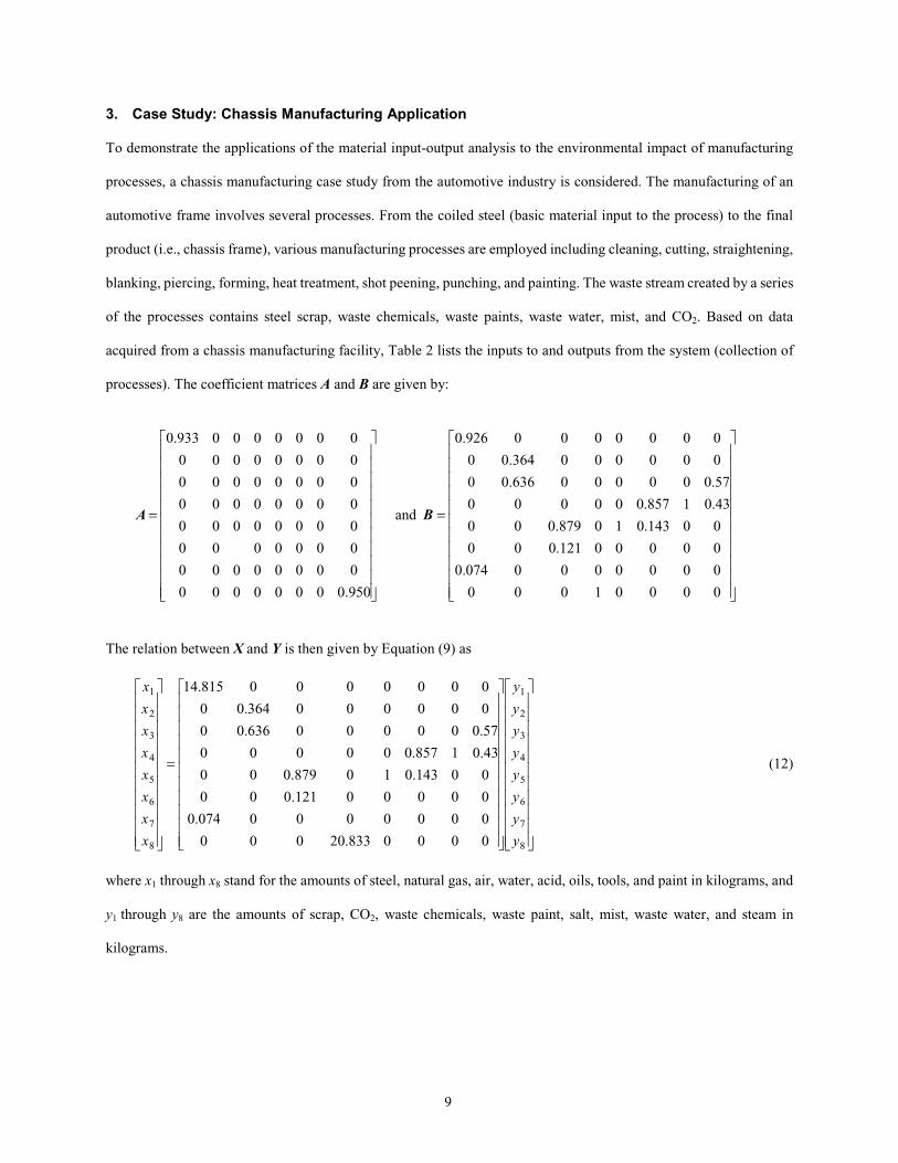
3. Case Study: Chassis Manufacturing Application

To demonstrate the applications of the material input-output analysis to the environmental impact of manufacturing

processes, a chassis manufacturing case study from the automotive industry is considered. The manufacturing of an

automotive frame involves several processes. From the coiled steel (basic material input to the process) to the final

product (i.e., chassis frame), various manufacturing processes are employed including cleaning, cutting, straightening,

blanking, piercing, forming, heat treatment, shot peening, punching, and painting. The waste stream created by a series

of the processes contains steel scrap, waste chemicals, waste paints, waste water, mist, and CO2. Based on data

acquired from a chassis manufacturing facility, Table 2 lists the inputs to and outputs from the system (collection of

processes). The coefficient matrices A and B are given by:

=

950.00000000

00000000

0000000

00000000

00000000

00000000

00000000

0000000933.0

A and

=

00001000

0000000074.0

00000121.000

00143.010879.000

43.01857.000000

57.000000636.00

000000364.00

0000000926.0

B

The relation between X and Y is then given by Equation (9) as

=

8

7

6

5

4

3

2

1

8

7

6

5

4

3

2

1

0000833.20000

0000000074.0

00000121.000

00143.010879.000

43.01857.000000

57.000000636.00

000000364.00

0000000815.14

y

y

y

y

y

y

y

y

x

x

x

x

x

x

x

x

(12)

where x1 through x8 stand for the amounts of steel, natural gas, air, water, acid, oils, tools, and paint in kilograms, and

y1 through y8 are the amounts of scrap, CO2, waste chemicals, waste paint, salt, mist, waste water, and steam in

kilograms.

10

Based on Equation (12), one can explore various possibilities to reduce the waste stream and drive the process toward

zero emission. For example, if it is desirable to reduce CO2 emissions by changing inputs, the corresponding gas and

air values can be determined from Figure 4. It also can be seen from Equation (12) that changes in several outputs may

depend on the same input. Figure 5 shows the relation between the input (acid) and the outputs (mist and waste

chemicals). The input acid level may then be specified to produce acceptable amounts of mist and waste chemicals.

Other input-output relations can be obtained in a similar fashion.

4. Aggregation of Material Input-output Models

If input-output models have been established for several processes operating in parallel, it might be desired to combine,

or aggregate, these models to understand the collective behavior of the processes. Care must be exercised in

undertaking this aggregation to avoid aggregation bias. For example, technical coefficients cannot simply be averaged,

since the input and output amounts may differ. To minimize or eliminate aggregation bias, aggregation should work

directly with the material inputs and outputs. The system boundary must also be selected carefully for the problem

under investigation so as to avoid excessive aggregation that may obscure model structures that reveal insights into the

underlying processes.

Based on the foregoing discussion, a methodology for aggregating material input-output models has been created to

combine process-level models. Such aggregation provides a broader region over which environmental performance

improvement opportunities can be pursued. Of course, if process-level material input-output models can be aggregated

to form an input-output model for a manufacturing system, further aggregation could then be performed to produce an

input-output model for an entire production facility. An aggregated material input-output model at the manufacturing

system, facility, or regional level can improve our ability to understand complex interactions by providing an insight

into relationship between the inputs and outputs. It also provides a method for harnessing input-output knowledge at

the process level to support the development of environmental input-output models at broader spatial levels.

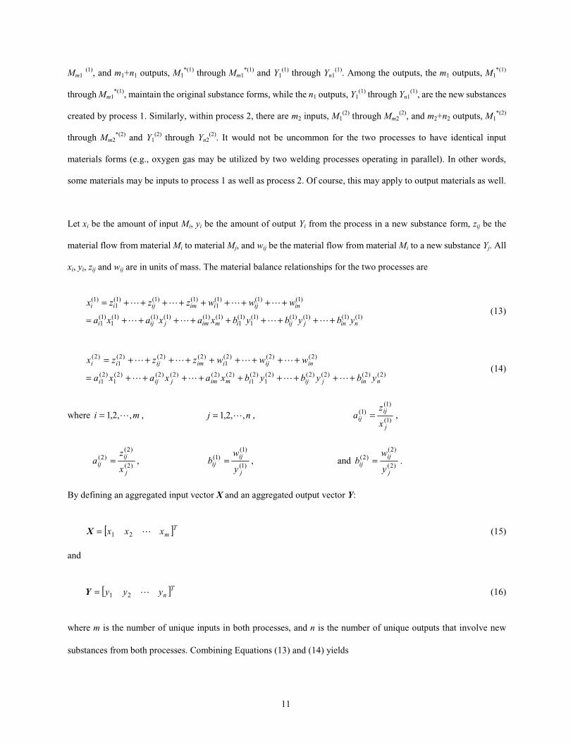
To aggregate material input-output models into a larger model, let us consider a fundamental case where two

manufacturing processes constitute a system, as shown in Figure 6. For process 1, there are m1 inputs, M1(1) through

11

Mm1 (1), and m1+n1 outputs, M1

*(1) through Mm1*(1) and Y1

(1) through Yn1(1). Among the outputs, the m1 outputs, M1

*(1)

through Mm1*(1), maintain the original substance forms, while the n1 outputs, Y1

(1) through Yn1(1), are the new substances

created by process 1. Similarly, within process 2, there are m2 inputs, M1(2) through Mm2

(2), and m2+n2 outputs, M1*(2)

through Mm2*(2) and Y1

(2) through Yn2(2). It would not be uncommon for the two processes to have identical input

materials forms (e.g., oxygen gas may be utilized by two welding processes operating in parallel). In other words,

some materials may be inputs to process 1 as well as process 2. Of course, this may apply to output materials as well.

Let xi be the amount of input Mi, yi be the amount of output Yi from the process in a new substance form, zij be the

material flow from material Mi to material Mj, and wij be the material flow from material Mi to a new substance Yj. All

xi, yi, zij and wij are in units of mass. The material balance relationships for the two processes are

)1()1()1()1()1(1

)1(1

)1()1()1()1()1(1

)1(1

)1()1()1(1

)1()1()1(1

)1(

ninjijimimjiji

inijiimijii

ybybybxaxaxa

wwwzzzx

+++++++++=

+++++++++=

LLLL

LLLL (13)

)2()2()2()2()2(1

)2(1

)2()2()2()2()2(1

)2(1

)2()2()2(1

)2()2()2(1

)2(

ninjijimimjiji

inijiimijii

ybybybxaxaxa

wwwzzzx

+++++++++=

+++++++++=

LLLL

LLLL (14)

where mi ,,2,1 L= , nj ,,2,1 L= , )1(

)1()1(

j

ijij

x

za = ,

)2(

)2()2(

j

ijij

x

za = ,

)1(

)1()1(

j

ijij

y

wb = , and

)2(

)2()2(

j

ijij

y

wb = .

By defining an aggregated input vector X and an aggregated output vector Y:

[ ]Tmxxx L21=X (15)

and

[ ]Tnyyy L21=Y (16)

where m is the number of unique inputs in both processes, and n is the number of unique outputs that involve new

substances from both processes. Combining Equations (13) and (14) yields

12

ninjijii

mimjijii

ininijijiiii

imimijijiiiii

ybybybyb

xaxaxaxa

wwwwwwww

zzzzzzzzx

++++++

+++++=

++++++++++

+++++++++=

LL

LL

LL

LL

2211

2211

)2()1()2()1()2(2

)1(2

)2(1

)1(1

)2()1()2()1()2(2

)1(2

)2(1

)1(1

(17)

where

)2()1(iii xxx += , and )2()1(

jjj yyy += .

The aggregated technical coefficients can be defined as follows:

)2()2()1()1(ijjijjij aaa αα += (18)

and

)2()2()1()1(ijjijjij bbb ββ += (19)

where )2()1()2()1( ,,, jjjj ββαα are weighting factors, j

jj x

x )1()1( =α ,

j

jj x

x )2()2( =α ,

j

jj y

y )1()1( =β , and

j

jj y

y )2()2( =β . It can

be seen that model aggregation does not introduce any bias. From Equations (13) through (19), an aggregated material

input-output model can be built with the following form:

BYAX 1)( −−= I , or ( )XABY −= − I1

where I is an m by m identity matrix, X is the aggregated input vector, and Y is the aggregated output vector defined by

Equation (15) and (16), A is the aggregated technical coefficient matrix, and B is the aggregated technical coefficient

matrix related to new substances from the underlying system.

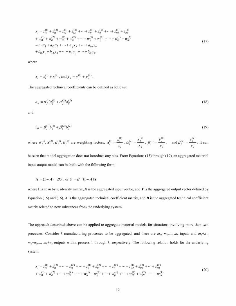
The approach described above can be applied to aggregate material models for situations involving more than two

processes. Consider k manufacturing processes to be aggregated, and there are m1, m2,..., mk inputs and m1+n1,

m2+n2,..., mk+nk outputs within process 1 through k, respectively. The following relation holds for the underlying

system.

)()2()1()()2()1()(1

)2(1

)1(1

)()2()1()()2()1()(1

)2(1

)1(1

kiNiNiN

kijijij

kiii

kiMiMiM

kijijij

kiiii

wwwwwwwww

zzzzzzzzzx

++++++++++++++

+++++++++++++=

LLLLL

LLLLL (20)

13

where M is the number of unique inputs in all k processes, and N is the number of unique outputs that involve new

generated substances from all k processes.

Correspondingly, aggregated technical coefficients are

)()()()()2()2()1()1( kij

kj

qij

qjijjijjij aaaaa αααα +++++= LL (21)

and

)()()()()2()2()1()1( kij

kj

qij

qjijjijjij bbbbb ββββ +++++= LL (22)

where )(qjα and )(q

jβ are weighting factors and have the following forms.

j

qjq

j x

x )()( =α (23)

j

qjq

j y

y )()( =β (24)

kq ,,2,1 L= .

As suggested by the above development, Equations (20) through (24) can be used to form a material input-output

model for a manufacturing system based on models for the individual processes. Using these relations, models for all

the production facilities operated by a company can be aggregated to form an input-output model for the company.

Similarly, the above methodology can support the aggregation of input-output models to create models at the industry

sector level, regional level, etc.

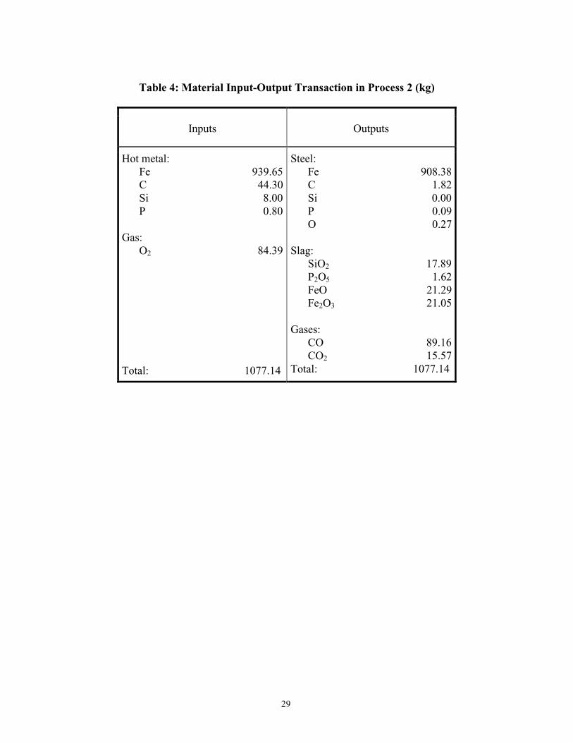
5. Application of the Aggregated Models in Steel-making

To illustrate the aggregation of material input-output models at the process level to form a model for a manufacturing

system, two steelmaking processes that operate in parallel within a production facility are used as an example. The two

steelmaking processes have different inputs and process operation control, and therefore the material outputs from the

two processes are different. The simplified material input-output transaction tables for the two processes are shown in

14

Tables 3 and 4, respectively [17]. The inputs to the process consist of hot metal, flux, and oxygen gas, while the

outputs from the process include steel, slag, fume, and gas. Fe, C, Si, P and O2, which form the X vector, are

considered inputs to the process. The new substances created by the process include FeO, Fe2O3, CO, CO2, SiO2, and

P2O5, which form the Y vector. In examining the table, CO and CO2 gases are significant discharges that have an

adverse environmental impact. The aim of the analysis presented here is to establish a linear multi-input multi-output

relationship through which opportunities to drive the process toward zero emission may be identified.

The aggregated input vector X and output vector Y are as follows.

[ ]2,,,, OPSiCFeT =X , and [ ]522232 ,,,,, OPSiOCOCOOFeFeOY T = .

It may be noted that the vector X includes all the unique material inputs while the vector Y includes all the unique

material outputs from the two processes. Then technical coefficient matrices of the two processes, based on Equations

(5) and (6), are

=

0071.00000

00000

003492.000

0000886.00

00009739.0

1A ,

=

05306.07265.05713.02913.00

000000

04694.00000

002735.04287.000

00007087.00

1B ,

=

0032.00000

01125.0000

00000

0000411.00

00009663.0

2A ,

=

5617.05324.07270.05712.03007.02226.0

4383.000000

04676.00000

002730.04288.000

00006993.07774.0

2B .

Using Equations (17) through (24) and A1, B1, A2, and B2, the aggregated technical coefficient matrices A and B can be

calculated as follows.

=

0050.00000

01125.0000

001726.000

0000639.00

00009703.0

A ,

=

5617.05317.07268.05712.02949.02226.0

4383.000000

04683.00000

002732.04288.000

00007051.07774.0

B .

15

Using Equation (9), it is possible to identify opportunities for reducing waste gases such as CO and CO2. For example,

assume that it is desirable to reduce the generation of CO and CO2 by 25 and 20 percent, respectively, i.e., the vector Y

is to be changed from [21.29 55.10 170.47 24.60 28.69 1.62]T to [21.29 55.10 127.85 19.68 28.69 1.62]T. Using

Equation (9), the vector X should be changed from [1865.22 85.26 15.79 0.80 153.54]T to

[1865.22 64.30 16.20 8.00 125.10]T. According to the I/O representation, the amount of input C should be reduced

from 85.26 to 64.30 kg. The result shows that the amount of carbon input into the process should be decreased. In

modern steelmaking practice, carbon is introduced in the form of coke in the blast furnace process. The carbon then

reduces FeO to produce elemental Fe and waste CO and CO2. Introducing more coke/carbon into the process, and

oversaturating the process with carbon, produces excessive levels of CO and CO2. Therefore, to implement an

environmentally friendly steelmaking process, control of the blast furnace process must avoid oversaturating the iron

with carbon. In this case, the input-output model has provided insight into how to improve the environmental

performance of the process. Of course, to implement the carbon reduction suggested by the input-output model

requires a careful technical analysis to assess the feasibility of the proposed change.

6. Discussion and Conclusions

Material input-output models provide a method to closely examine environmental impacts of manufacturing activities

at the process level. An aggregated material input-output model permits identification of opportunities to improve the

environmental performance and drive manufacturing systems toward zero emissions at larger spatial scales (e.g., the

facility level). However, care should be exercised when responding to changes suggested by input-output models, as

the feasibility of the changes must be carefully assessed for the process or system under study. For example, an

input-output model may suggest that it is mathematically possible to determine the process input X, using the design

equation, if a desired material output vector, Y, is specified. The model indicates that if the material inputs are changed,

the desired outputs will be obtained. However, further investigation must be undertaken to assess the

feasibility/efficacy of such changes. If such an investigation reveals that such changes are not feasible or will be

ineffective, it is very likely that the investigation will reveal alternative approaches like substitute processes, process

layout improvements, process control, and alternative processing materials [18, 19] that will produce environmental

benefits within the underlying manufacturing process/system. Of course structural changes in the process will change

elements of the technical coefficient matrices A and B, which in turn change the behavior of the underlying system.

16

There are several opportunities for reducing the environmental impact associated with manufacturing processes and

systems:

• changes in inputs to processes when desirable outputs are specified, provided that the specified process conditions

are feasible.

• changes in the technical coefficients of the underlying process.

It should be noted that while the input-output analysis provides a tractable method of identifying opportunities to

reduce the environmental impact, a more complex model may be necessary for those manufacturing processes with

nonlinear input-output relations. In addition, not all manufacturing process may be best modeled with an input-output

format [20]. Based on the analysis of process characteristics, an appropriate modeling strategy should be employed. It

should also be pointed out that process changes may affect material yield, productivity, and product quality

characteristics. As noted above, manufacturers must thoroughly investigate consequences and side-effects when

input-output analysis identifies promising opportunities for emission reduction/elimination.

Some conclusions can be drawn from the above analysis and discussion:

• The proposed environmental input-output analysis of manufacturing processes is helpful in understanding the

dependence of the environmental impact on the process inputs. It tracks material flow in the entire process and

provides clues as to how to drive the manufacturing processes and systems toward zero emission.

• Opportunities for reducing the environmental impact of manufacturing processes may include changes to the

inputs of the process, and changes in the technical coefficients of the processes. The implementation of the latter

needs to use specific process knowledge and techniques.

A methodology for aggregation of material input-output models at the process level has been developed. Material

input-output models of manufacturing processes can be aggregated into a system model without bias. It is possible to

further aggregate such models into a material input-output model for systems at larger spatial scales. The aggregated

material input-output model provides a means to support improvement opportunity analysis of the environmental

performance of manufacturing systems and production facilities.

17

7. Acknowledgement

The authors gratefully acknowledge support from the NSF/EPA Partnership for Environmental Research (NSF No.

DMI-9613076) and (EPA No. R825345), and Michigan Technological University. We would like to acknowledge the

assistance of Profs. Walter Olson (University of Toledo) and S. M. Pandit for their input during the early stages of this

work.

8. References

[1] NAE. Committee on Industrial Environmental Performance Metrics, Industrial Environmental Performance

Metrics, National Academy Press, 1999.

[2] Munoz, AA, Sheng P. An Analytical Approach for Determining the Environmental Impact of Machining

Processes. Journal of Materials Processing Technology 1995;53:736-58.

[3] Choi ACK, Kaebernick H, Lai WH. Manufacturing Processes Modeling for Environmental Impact Assessment.

Journal of Materials Processing Technology 1997;70:231-38.

[4] Bauer, DJ, Thurwachter S, Sheng P. Integration of Environmental Factors in Surface Planning: Part 1- Mass and

Energy Modeling. Transactions of NAMRI/SME 1998;XXVI:171-6.

[5] Leontief W. Input-Output Economics. New York: Oxford University Press, 1986.

[6] Breuil JM. Input-Output Analysis and Pollutant Emissions in France. The Energy Journal 1992;13(3).

[7] Hawdon D, Pearson P. Input-Output Simulations of Energy, Environment, Economy Interactions in the UK

Energy Economics 1995;17(1):73-86.

[8] Lave LB, E.Cobas-Flores, Hendrickson CT, McMichael FC. Using Input-Output Analysis to Estimate

Economy-wide Discharges. Environmental Science & Technology 1995; 29(9):420A-26A.

[9] Miller RE, Blair PD. Input-Output Analysis: Foundations and Extensions, Englewood Cliffs, NJ:Prentice-Hall,

1985.

[10] Milacic D, Gowaikar H, Olson WW, Sutherland JW. A Proposed LCA Model of Environmental Effects with

Markovian Decision Making. Proceedings of the 1997 Total Life Cycle Conference -Life Cycle Management and

Assessment (Part1), 1997:111-8.

[11] Hatanaka M. Note on Consolidation within a Leontief System. Econometrica 1952;20(2):301-03.

18

[12] Balderston JB, Whitin TM. Aggregation in the Input-Output Model. Economic Activity Analysis, In: Economic

Activity Analysis, Ed. Morgenstern O, New York:John Wiley & Sons, 1999:79-128.

[13] Caber B, Contreras D, Miravete EJ. Aggregation in Input-Output Tables: How to Select the Best Cluster

Linkage. Economic System Research 1991:99-109.

[14] Morimoto Y. On Aggregation Problems in Input-Output Analysis. Review of Economic Studies 1970;

37(109):119-26.

[15] Olsen A. Aggregation in Macroeconomic Models: an Empirical Input-Output Approach. Working Paper, 1999,

http//www.dreammodel.dk/pdf/W1999_02.pdf.

[16] Theil H. Linear Aggregation in Input-output Analysis. Econometrica 1957;25(1):111-22.

[17] Xue H, Kumar V, Pandit SM, Sutherland JW. An Enhanced Input-Output Model for Material Flow Analysis of

Manufacturing Processes. Proc. of 2004 JUSFA, 2004.

[18] Garner A, Keoleian GA. Industrial Ecology: an Introduction. 1995.

[19] Sutherland JW, Gunter KL. Chapter 13: Environmental Attributes of Manufacturing Processes. Handbook of

Environmentally Conscious Manufacturing, Ed. Christian N. Madu, Kluwer Academic Publishers, 2001:293-16.

[20] Xue H, Filipovic A, Pandit SM, Sutherland JW, Olson WW. Using a Manufacturing Process Classification

System for Improved Environmental Performance, Proc. of the 2000 SAE International Congress and Exposition:

Environmental Concepts for the Automotive Industry, 2000:23-30.

19

Author Vitae

Dr. Huanran Xue was born in China. He received his B.S. and M.S. degrees from the Huazhong

University of Science and Technology, China, and Ph.D. degree in the Department of Mechanical

Engineering - Engineering Mechanics from Michigan Technological University. He currently

works for Ford Motor Company Manufacturing Design Center as a system analyst. He works in

the CAD/CAM area for stamping engineering.

Vishesh Kumar is a Ph.D. candidate in the Department of Mechanical Engineering - Engineering

Mechanics at Michigan Technological University and a Graduate Scholar of the Michigan Tech

Sustainable Futures Institute. He received his B.Tech in Mechanical Engineering from IIT Kanpur

in 2000. Prior to coming to Michigan Tech, he worked as a research engineer for an Indian

automotive manufacturer. Mr. Kumar has published numerous papers in various journal and

conference proceedings. His research is focused on the economic sustainability of the automotive

recycling infrastructure and value recovery at the end-of-use stage of the product life cycle.

Dr. John W. Sutherland holds the Henes Chair Professorship within the Department of Mechanical

Engineering – Engineering Mechanics and serves as the Co-Director of the Sustainable Futures

Institute at Michigan Technological University. He received his Ph.D. from the University of

Illinois at Urbana-Champaign in 1987. Prior to joining the faculty at Michigan Tech in 1991, he

served as Vice President of a small manufacturing consulting company. His research and teaching

interests are focused on design and manufacturing for sustainability. He has mentored over 60

students to the completion of their degrees and has authored/co-authored over 200 publications. Dr.

Sutherland and his students are the recipients of numerous awards for education and research.

20

Production Facility Pollutant releases

Manufacturing Process

Supply Chain Network

Figure 1: Manufacturing Processes, Production Facilities, and Supply Chain Network

21

Mm*

Yn

Process

Manufacturing

M1*

M2*M1

M2

Mm

Y1

Figure 2: Input-Output Relation of a Manufacturing Process

22

system boundary

inflows outflows

Figure 3: Material Flows in Manufacturing Processes

23

6000

5550

5000

4500

4000

3500

3000

2500

6000500040003000200010000

natural gas

air

natural gas & air (kg)

current combination

Figure 4: Output CO2 vs. Inputs Natural Gas and Air

24

350

300

250

200

1501700165016001550150014501400

acid (kg)

1650

1600

1550

1500

1450

mist

waste chemicals

Figure 5: Outputs Mist and Waste Chemicals vs. Input Acid

25

Process 1

M1(1)

M2(1)

Mm1(1)

M1*(1)

Mm1*(1)

Y1(1)

Yn1(1)

---

---

---

Process 2

M1(2)

M2(2)

Mm2(2)

M1*(2)

Mm2*(2)

Y1(2)

Yn2(2)

---

---

---

Figure 6: Aggregation of Multiple Manufacturing Processes

26

Table 1: Input-Output Transaction for a Process

Outputs

M1* M2

* ... Mm* Y1 ... Yn

M1 z11 z12 ... z1m w11 ... w1n

M2 z21 z22 ... z2m w21 ... w2n

... ... ... ... ... ... ... ...

Inputs

Mm zm1 zm2 ... zmm wm1 ... wmn

27

Table 2: Input-Output Transaction for Manufacturing of Frame (kg)

St

eel

Nat

ural

G

as

Air

H2O

Aci

d

Oils

Too

ls

Pain

t

Scra

p

CO

2

Was

te

chem

.

Was

te

pain

t

Salt

Mis

t

Was

te

H2O

Stea

m

Tot

al

Steel 37500 2500 40000

Natural Gas

2000

2000

Air 3500 2250 5750

Water 300 28000 1700 30000

Acid 1450 200 50 1700

Oils 200 200

Tools 200 200

Paints 12.31 0.62 12.93

Total 37500 0 0 0 0 0 0 12.31 2700 5500 1650 0.62 200 350 28000 3950 79862.93

28

Table 3: Material Input-Output Transaction in Process 1 (kg)

Inputs Outputs

Pig Iron: Fe 925.57 C 40.96 Si 7.79

Gas:

O2 69.15

Total: 1043.47

Steel: Fe 901.44 C 3.63 Si 2.72

Slag:

SiO2 10.80 Fe2O3 34.05

Gases:

O2 0.49 CO 81.31 CO2 9.03

Total: 1043.47

29

Table 4: Material Input-Output Transaction in Process 2 (kg)

Inputs Outputs

Hot metal: Fe 939.65 C 44.30 Si 8.00 P 0.80

Gas:

O2 84.39

Total: 1077.14

Steel: Fe 908.38 C 1.82 Si 0.00 P 0.09 O 0.27

Slag:

SiO2 17.89 P2O5 1.62 FeO 21.29 Fe2O3 21.05

Gases:

CO 89.16 CO2 15.57

Total: 1077.14