Material Balance Notes

MATERIAL BALANCE NOTES

Revision 3

Irven Rinard

Department of Chemical EngineeringCity College of CUNY

and

Project ECSEL

October 1999

© 1999 Irven Rinard

i

CONTENTS

INTRODUCTION 1A. Types of Material Balance ProblemsB. Historical Perspective

I. CONSERVATION OF MASS 5A. Control VolumesB. Holdup or InventoryC. Material Balance BasisD. Material Balances

II. PROCESSES 13A. The Concept of a ProcessB. Basic Processing FunctionsC. Unit OperationsD. Modes of Process Operations

III. PROCESS MATERIAL BALANCES 21A. The Stream SummaryB. Equipment Characterization

IV. STEADY-STATE PROCESS MODELING 29 A. Linear Input-Output Models

B. Rigorous Models

V. STEADY-STATE MATERIAL BALANCE CALCULATIONS 33A. Sequential ModularB. SimultaneousC. Design SpecificationsD. OptimizationE. Ad Hoc Methods

VI. RECYCLE STREAMS AND TEAR SETS 37A. The Node Incidence MatrixB. Enumeration of Tear Sets

VII. SOLUTION OF LINEAR MATERIAL BALANCE MODELS 45A. Use of Linear Equation SolversB. Reduction to the Tear Set VariablesC. Design Specifications

-0-

VIII. SEQUENTIAL MODULAR SOLUTION OF NONLINEAR 53 MATERIAL BALANCE MODELS

A. Convergence by Direct IterationB. Convergence AccelerationC. The Method of Wegstein

IX. MIXING AND BLENDING PROBLEMS 61A. MixingB. Blending

X. PLANT DATA ANALYSIS AND RECONCILIATION 67A. Plant DataB. Data Reconciliation

XI. THE ELEMENTS OF DYNAMIC PROCESS MODELING 75A. Conservation of Mass for Dynamic SystemsB. Surge and Mixing TanksC. Gas Holders

XII. PROCESS SIMULATORS 87A. Steady StateB. Dynamic

BILIOGRAPHY 89

APPENDICES

A. Reaction Stoichiometry 91B. Evaluation of Equipment Model Parameters 93C. Complex Equipment Models 96D. Linear Material Balance by Spreadsheet - Example 97E. The Kremser Model of Gas Absorbers 98

-1-

INTRODUCTION Revised October 2, 1999

The material balance is the fundamental tool of chemical engineering. It is the basis forthe analysis and design of chemical processes. So it goes without saying that chemical engineersmust thoroughly master its use in the formulation and solution of chemical processing problems.

In chemical processing we deal with the transformation of raw materials of lower valueinto products of higher value and, in many, cases unwanted byproducts that must be disposed of.In addition many of these chemical compounds may be hazardous. The material balance is thechemical engineer's tool for keeping track of what is entering and leaving the process as well aswhat goes on internally. Without accurate material balances, it is impossible to design or operatea chemical plant safely and economically.

The purpose of these notes is to provide a guide to the use of material balances inchemical engineering. Why one might ask? Aren't there already enough books on the subject,books such as those by Felder and Rouseau, by Himmelblau, and by Reklaitis? To answer thatquestion we need to look briefly at the history of the problem.

A. Types of Material Balance Problems

First let us look at the types of material balance problems that arise in chemicalengineering. There are four basic types of problems:

(1) Flow sheet material balance models for continuous processes operating in the steady state,

(2) Mixing and blending material balances, (3) Flow sheet material balances for non-steady state processes, either continuous or

batch, and

(4) Process data analysis and reconciliation

A flow sheet is a schematic diagram of a process which shows at various levels of detailthe equipment involved and how it is interconnected by the process piping (See, for instance Figures II-1 and II-2 in Chapter II). A flow sheet material balance shows the flow rates andcompositions of all streams entering and leaving each item of equipment.

Most of the emphasis on material balance problems has been on continuous processesoperating in the steady state. Again one might ask why. The reason is simple. Of the totaltonnage of chemicals produced, the vast majority is produced using continuous steady-stateprocesses. This includes oil refineries as well as chemical plants producing large tonnage productssuch as sulfuric acid, ethylene, and most of the other commodity chemicals, petrochemicals and

-2-

polymers. It has been found that the most economical and efficient way to produce suchchemicals on a large scale is via the continuous process operating in the steady-state. This is thereason for the emphasis on this type of material balance problem.

Another class of material balance problems is those involving blending and mixing. A sub-stantial number of the products produced by the chemical processing industries are blends or mix-tures of various constituents or ingredients. Examples of blends are gasoline and animal feeds; ofprecise mixtures, prescription drugs and polymeric resins.

Dynamic material balance problems arise in the operation and control of continuousprocesses. Also, batch processes, by their very nature, are dynamic. In either case we mustconsider how the state of the process varies as a function of time. In addition to determining theflow rates and compositions of the interconnecting streams, we must also follow the changes ininventory within the process itself.

In the three types of problems just discussed, we are interested in predicting theperformance of the process or equipment. Our models start by assuming that the law ofconservation of mass is obeyed. A fourth type of problem, which encountered by engineers in theplant, starts with actual operating data, generally flow rates and compositions of various streams. The problem is to determine the actual performance of the plant from the available data.

This, in many ways, is a much more difficult problem than the first three. Why? Simple. The data may in error for one reason or another. A flow meter may be out of calibration orbroken entirely. A composition measurement is not only subject to calibration errors but samplingerrors as well. Thus the first thing one must do when dealing with plant data is to determine, ifpossible, whether or not it is accurate. If it is, then we can proceed to use it to analyze it todetermine process performance. If not, we must try to determine what measurements are in error,by how much, and make the appropriate corrections to the data. This is known as datareconciliation and is possible only if we have redundant measurements.

B. Historical Perspective

The solution of material balance problems for continuous steady-state processes of anycomplexity used to be very difficult. By its nature, the problem is one of solving a large numberof simultaneous algebraic equations, many of which are highly nonlinear. Before the availabilityof computers and the appropriate software, the solution of the material balance model for achemical process typically took a team of chemical engineers using slide rules and addingmachines days or weeks, if not months. And given the complexity of the problem, errors werecommon.

The methods used in those days to solve material balance problems days are best describedas ad hoc. Typically an engineer started with the process specifications such as the production

-3-

rate and product quality and calculated backwards through the process. Intermediate specifi-cations would be used as additional starting points for calculations. As will be seen later in thesenotes, such an approach goes against the output-from-input structure of the process and can leadto severe numerical instabilities.

The growing availability of digital computers in the late 1950's led to the development ofthe first material balance programs such as IBM's GIFS, Dartmouth's PACER and Shell’sCHEOPS. Almost every major oil and chemical company soon developed in-house programs ofwhich Monsanto's Flowtran is the best-known example. By the 1970's several companiesspecializing in flow sheet programs had come into existence. Today companies such asSimulation Sciences, Aspen Technology and Hyprotech provide third-generation versions ofsteady-state flow sheet simulation programs that provide a wide range of capabilities and arerelatively easy to use compared to earlier versions.

Dynamic simulation is less advanced than steady-state simulation. This is due, in part, tothe lack of emphasis until recently on the dynamic aspects of chemical engineering operations. This situation is changing rapidly due to demands for improved process control and for simulatorsfor training operating personnel. The companies mentioned in the previous paragraph have allrecently added dynamic simulators to their product lines. In addition several companies such asABB Simcon offer training simulators for the process industries.

C. Material Balance Methodology

There are two major steps involved in applying the principle of conservation of mass tochemical processing problems. The first is the formulation of the problem; the second, its solu-tion.

By formulation of the problem is meant determining the appropriate mathematicaldescription of the system based on the applicable principles of chemistry and physics. In the caseof material balances, the appropriate physical law is the conservation of mass. The resulting set ofequations is sometimes referred as a mathematical model of the system.

What a mathematical model means will be made clearer by the examples contained in thesenotes. However, some general comments are in order. First, there may be a number of mathe-matical models of varying levels of detail that can apply to the same system. Which we usedepends upon what aspects of the process we wish to study. This will also become clearer as weproceed. Second, for many systems of practical interest, the number of equations involved in themodel can be quite large, on the order of several hundred or even several thousand.

Thus, the process engineer must have a clear of how to formulate the model to insure thatit is a correct and adequate representation of the process for the purposes for which it is intended. This is the subject of Sections I - IV of these notes.

Today, using process simulation program such as PRO-II, ASPEN, and HYSIM, a single

-4-

engineer can solve significant flow sheeting problems in as little as a day or two and, moreover,do it much more accurately and in much more detail than was previously possible. The processengineer can now concentrate on the process model and the results rather than concocting ascheme to solve the model equations themselves. The simulation program will do that, at leastmost of the time. However, things do go wrong at times. Either the problem is very difficult forthe simulator to solve or a mistake has been made in describing the process to the program. Thus,in order to fix what is wrong, the engineer does need to know something about how the simula-tion program attempts to solve the problem. This is the subject of Sections V, VIII, and IX ofthese notes. Steady-state simulation programs are described briefly in Section XII.

Simple material balance problems involving only a few variables can still be solvedmanually. However, it is generally more efficient to use a computer program such as a spread-sheet. Both approaches are discussed in Section VII.

In order to achieve high levels of mass and energy utilization efficiency, most processesinvolve the use of recycle. As will be seen, this creates recycle loops within the process whichcomplicate the solution of material balances models for the process. A systematic procedure foridentifying recycle loops is presented in Section VI.

An introduction to problems encountered in determining plant performance from plant isgiven in Section X.

There are two basic process operating modes that are of interest to chemical engineers,dynamic and steady state. All processes are dynamic in that some or all of the process variableschange with time. Many processes are deliberately run dynamically; batch processes being theprime example. However, many large-scale processes such as oil refineries and petrochemicalplants are run in what is called the continuous or steady state operation. The appropriate modelfor dynamic processes are differential equations with respect to time. In general, continuous pro-cesses operating in the steady state are modeled by algebraic equations. Dynamic processmodeling is discussed briefly in Section XI and dynamic process simulators in Section XII.

Many topics in process modeling are not covered in these notes. The most seriousomission is the companion to the material balance, namely, the energy balance. Also, little atten-tion is paid to what are known as first-principle or rigorous equipment models. Such modeling ismore properly covered in texts and courses on unit operations and chemical reaction engineering. However, a few of the simpler and more useful models are given in Appendix E.

-5-

I. CONSERVATION OF MASS

Revised October 2, 1999

The principle of conservation of mass is fundamental to all chemical engineering analysis. The basic idea is relatively easy to understand since it is fact of our everyday life.

Let us consider a simple example. Suppose we are required to prepare one kilogram of asolution of ethanol in water such that the solution will contain 40% ethanol by weight. So, weweigh out 400 grams of ethanol and 600 grams of water and mix the two together in a largebeaker. If we weigh the resulting mixture (making appropriate allowance for the weight of thebeaker), experience says it will weigh 1000 grams or one kilogram. And it will. This is amanifestation of the conservation of mass.

That, in the absence of nuclear reactions, mass isconserved is a fundamental law of nature.

This law is used throughout these notes and throughout all chemical engineering.

Suppose we happened to measure the volumes involved in making up our alcoholsolution. Assuming that we do this at 20 C, we would find that we added 598.9 ml of water to315.7 ml of ethanol to obtain 935.2 ml of solution. However, the sum of the volumes of the purecomponents is 914.6 ml. We conclude that volume is not conserved.

Let us take note of one other fact about our solution. If we were to separate it back intoits pure components (something we could do, for instance, by azeotropic distillation) and did thiswith extreme care to avoid any inadvertent losses, we would obtain 400 gm of ethanol and 600gm of water. Thus, in this case, not only was total mass conserved but the mass of each of thecomponents was also.

This is not always true. Suppose that instead of adding ethanol and water, we added(carefully and slowly) sodium hydroxide to sulfuric acid. Suppose that the H2SO4 solutioncontains exactly 98.08 pounds of H2SO4 and that we add exactly 80.00 pounds of NaOH. Achemical reaction will take place as follows:

H2SO4 + 2 NaOH à Na2SO4 + 2 H2O.

Notice that the amount of H2SO4 in the original solution is 1.0 lb-mol and that the amount ofNaOH added is exactly 2.0 lb-mols. What we are left with is 1.0 lb-mol of Na2SO4 or 142.05 lbsand 2.0 lb-mols of H2O or 36.03 lbs. No individual component is conserved; the H2SO4 and theNaOH have disappeared and in their place we have Na2SO4 and H2O. However, if we look at theatomic species H, O, S, and Na, we will find that these are all con-served. That is exactly whatthe reaction equation expresses.

-6-

Thus we have to be careful to identify the appropriate conserved species for the system weare analyzing. If no chemical reactions are involved, then each of the molecular species isconserved. If chemical reactions are involved, then only atomic species are conserved. There willbe a mass balance for each of the conserved species. In the example above it does not make muchdifference since there are four conserved atomic species and four molecular species. But, ifadditional reactions take place involving, say, Na2S and NaHSO4, then the number of molecularspecies exceeds the number of conserved atomic species. This will generally be the case.

A. Control Volumes

We apply the principle of the conservation of mass to systems to determine changes in thestate of the system that result from adding or removing mass from the system or from chemicalreactions taking place within the system. The system will generally be the volume containedwithin a precisely defined section of a piece of equipment. We refer to this precisely definedvolume as a control volume.

It may be the entire volume of the equipment. This would be the case if the system is acylinder containing a gas or gas mixture. Or it may be the volume associated with a particularphase of the material held within the system. For instance, a flash drum is used to allow a mixtureof vapor and liquid to separate into separate vapor and liquid phases. The liquid phase willoccupy part of the total volume of the drum; the vapor, the remainder of the volume. If we areinterested only in what happens to the liquid phase, then we would specify the volume occupiedby the liquid as our control volume.

Note that the control volume can change over the course of an operation. Suppose we areadding liquid to a tank that contains 100 Kg of water to start with and that we add another 50 Kg. The tank would originally contain 100 liters of water but would contain 150 liters after theaddition. On the other hand, if our interest is in the entire contents of the tank - both the liquidand the vapor in the space above it - then we would take the volume of the tank itself as ourcontrol volume. This volume, of course, will not change.

B. Holdup or inventory

Another concept that we will need to make precise is that of holdup, also known asinventory or accumulation. Holdup refers to the amount of a conserved species contained withina control volume. We can refer to the total holdup as simply the total mass of material containedwithin the control volume. Or we can refer to the holdup of a particular component, sodiumchloride say, which is contained within the control volume. Needless to say, the sum of theholdups of all of the individual components within the control volume must equal the total hold-up.

-7-

C. Material Balance Basis

Whenever we apply the principle of conservation of mass to define a material balance, wewill want to specify the basis for it. Generally, the basis is either the quantity of total mass or themass of a particular component or conserved species for which the material balances will bedefined. Or, for continuous processes, it might be the mass flow rate of a component orconserved species.

Quite often the basis will be set by the specification of the problem to be solved. Forinstance, if we are told that a tank contains 5,000 pounds of a particular mixture about whichcertain questions are to be answered, then a natural basis for the problem would the 5,000 poundsof the mixture. Or, if we are looking at a continuous process to make 10,000 Kg/hr of ethanol, a reasonable choice for a basis would be this production rate.

Some problems, however, do not have a naturally defined basis so we must choose one. For instance, if we are asked what is the mass ratio of NaOH to H2SO4 required to produce aneutral solution of NaCl in water, we would have to specify a basis for doing the calculations. We might choose 98.08 Kg of H2SO4 (1.0 Kg-mol) as a basis. Or we could chose 1.0 lb ofH2SO4. Either is acceptable. One basis may make the calculations simpler than another, but inthis day of personal computers the choice is less critical than it might have been years ago. Whatever the choice of basis, it is mandatory that all material balances are defined to be consistentwith it.

D. Material Balances

We are now in a position to define material balances for some simple systems. (Note: Material balances are sometimes referred to as mass balances.) There are three basic situationsfor which we will want to do this:

1) A discrete process in which one or more steps are carried out over a finite butindefinite period of time.

An example of such a process is the dissolving of a specified quantity of salt in a quantityof water contained in a tank. We are only interested in the concentration in weight % of the saltin the water after it is completely dissolved and not how long it takes for the salt to dissolve.

2) A continuous process operating in the steady state.

By definition, continuous process operating in the steady state undergoes no changes in itsinternal state variables such as temperatures, pressures, compositions, and liquid levels. Inaddition, all the flow rates of all streams entering and leaving each item of equipment are constant. What this means from the standpoint of material balances is that there is no change in any of theholdups in the system.

-8-

3) Dynamic processes.

This is the general case in which both the holdups within equipment as well as the flowrates and compositions of the input and output streams can vary with time. This type of massbalance is discussed in more detail in Section XI.

Examples

a. Discrete process

Let us now consider the application of the principle of the conservation of mass to adiscrete process. For each of the conserved species, it can be stated as follows:

(I-1) Change in holdup = additions to the control volume- withdrawals from the control volume

Consider the following example:

We have a tank that initially holds 100 Kg of a solution containing 40% by weight of saltin water.

(1) We add 20 Kg of salt to the tank and allow it to dissolve.What do we now have in the tank?

First we have to identify the conserved species. Since there are no chemical reactionsinvolved, both salt and water are conserved species. Next we have to define the control volume. It seems natural to choose the salt solution in the tank. Our basis is the amount of solutionoriginally contained in the tank.

Now we can define a material balance for each conserved species as follows:

Water

Initial holdup of water = (1 - 0.4)(100) = 60 Kg

Change in holdup of water = additions of water to the control volume - withdrawals of water from the control volume

Since no water is either added or withdrawn, the change in this holdup is zero. Therefore theholdup of water after the salt addition is still 60 Kg.

SaltInitial holdup of salt = (0.4)(100) = 40 Kg

-9-

Change in holdup of salt = additions of salt to the control volume - withdrawals of salt from the control volume

We add 20 Kg of salt and withdraw no salt. Therefore the change in the holdup of salt = +20Kg and the holdup of salt after the addition is 40 + 20 = 60 Kg. A simple calculation shows thatthe concentration of salt in the tank is now 50 weight %.

(2) We withdraw 40 Kg of the solution now in the tank.

Since the solution in the tank is 50 weight % salt and 50 weight % water, in withdrawing40 Kg of solution, we will withdraw 20 Kg of salt and 20 Kg of water. This will leave 60 - 20 =40 Kg of each component in the tank. The composition has not changed from Step 1.

b. Continuous steady-state process

Let us consider a continuous mixer which has two input streams and, of course, oneoutput stream (See Figure 6 for a diagram). Suppose the first input stream has a flow rate of10000 lb/hr of a 40 wt. % solution of salt in water while the second input stream has a flow rateof 20000 lb/hr of a 70 wt. % solution of salt in water. What is the flow rate and composition ofthe output stream?

Since the system is now characterized in terms of rates of flow into the control volume(additions) and rates of flow out of the system (withdrawals), we need to restate the principle ofconservation of mass as follows:

(I-2) Rate of change of holdup = rate of additions to the control volume - rate of withdrawals from the control volume

For a continuous system operating in the steady state, the holdup does not change with time. Therefore, the rate of change of holdup is zero and Eqn. I-2 becomes

(I-3) Rate of withdrawals from the control volume = Rate of additions to the control volume

Let us apply this to the mixer problem. The control volume is the contents of the mixer (eventhough these do change) and the basis is the total rate of flow to the mixer. As in the previousexample, the conserved species are salt and water.

Salt

-10-

Fin

Fout

z

Rate of withdrawal of salt =

rate of additions of salt to the mixer

Rate of additions = (10000)(0.4) + (20000)(0.7) = 18000 lb/hr of salt

Water

Rate of withdrawal of water =rate of additions of water to the mixer

Rate of additions = (10000)(0.6) + (20000)(0.3) = 12000 lb/hr

Thus the stream leaving the mixer has a flow rate of 18000 lb/hr of salt and 12000 lb/hr of water,for a total of 30000 lb/hr. This is exactly the total flow rate of the mixer output we get by addingup the total flow rates to the mixer. Also, the composition of salt of the stream leaving the mixer=

(100)(18000)/(30000) = 60 wt %.

c. Dynamic Process

Consider the surge tank shown in Figure I-1. Water flows into the tank with a flow rate Fin lb/hr. Itflows out at a rate Fout lb/hr. The flow rates in andout can be adjusted by means of the valves in the inletand outlet piping. The tank has the form of anupright cylinder that has a cross section area of S ft2. The liquid level in the tank is z ft.

We know from experience that if the flowrates in and out are not exactly equal, the level in thetank will change with time. If the inlet flow rateexceeds the outlet flow rate, then the level will riseand vice versa. Now, the purpose of a surge tank isto absorb changes in the inlet flow rate whilemaintaining a relatively constant outlet flow rate. (The reservoirs that supply water to a town or cityare surge tanks where the inlet flow is the run-off from rainstorms and the outlet flow Figure I-1. Surge Tankis the daily consumption by the town or city.) Thus, a question that designers of surge tanks mustask is, given an estimate of the variations of inlet and outlet flow rates as functions of time, how

-11-

big must the surge tank be so that it never runs dry (town loses its water supply) or neveroverflows (area surrounding the reservoir is flooded). In general this is a complex design problembut let us look at a simple example to at least illustrate the concept.

Suppose that under normal conditions the level in the tank is to be half the height of thetank. If the flow rate into the tank becomes zero for a period of time (no rain), how long will ittake for the tank to run dry if the outlet flow rate is maintained at its usual value? Specifically,suppose that the cross section area of the tank is 10 ft2 and its height is 10 ft and the normal outletflow rate is 12,480 lb/hr.

First, let us take the volume of liquid in the tank as the control volume. The holdup ofwater in the control volume will be

Holdup = Szρ, where ρ is the density of water (62.4 lb/ft3).

Consider an interval of time ∆t. Suppose that over that time interval the inlet and outlet flowrates are constant but not necessarily equal. Then, by the conservation of mass the change in theholdup will be given by

(I-1) Holdup|t=�t - Holdup|t=0 = Fin ∆t - Fout ∆t

Now, if we divide both sides of the mass balance equation (Eqn. I-1) by ∆t and take the limit as∆t -> 0, we get the differential form of the mass balance, to wit,

(I-2) d[Szρ]/dt = Fin - Fout

If we assume that � is constant (a reasonable assumption if the temperature is also reasonablyconstant), then our mass balance equation becomes

(I-3) dz/dt = (Fin - Fout)/Sρ

For our problem Fin = 0 and Fout = 12,480 lb/hr, both constant. We can calculate dz/dt, that is

dz/dt = (0 - 12480)/(10)(62.4) = -20 ft/hr.

Since the nominal level is 5.0 ft (half the tank height of 10ft), it will take 0.25 hour or 15 minutesfor the tank to run dry.

Further examples of the application of the principle of conservation of mass, particularlyfor reacting systems, will be found in the subsequent sections of these notes.

-12-

II. PROCESSES


A. The Concept of a Process

-13-

Processes are the main concern of chemical engineers. A process is a system that convertsfeedstocks of lower intrinsic value to products of higher value. For instance, the block diagram ofa process to manufacture ammonia from natural gas is shown in Figure II-1. This process hasseveral sections, each one of which carries out a specific task and is, in effect, a mini-process. Natural gas, steam and air are fed to the Reformer Section that converts these feeds into a mixtureof H2, CO,

Fig. II-1. Block Diagram for Ammonia Process

CO2, N2, and H2O. The overall chemical reactions involved are:

CH4 + H2O à CO + 3 H2

CH4 + O2 à CO + 2 H2

CH4 + 2 O2 à CO2 + 2 H2O.

Since H2 is the desired raw material from which to make ammonia, this gas mixture is sentto the CO Shift Section where additional steam is added to improve conversion by the water gasshift reaction:

CH4

Steam

Air Steam

MethaneReformer

Water GasShift

Converter

CO2Removal

CO2H2O

ArgonPurge

Methanation

COCO2H2

H2ON2

CH4Ar

COH2N2

CH4Ar

SYN GASH2N2

CH4ArNH3

ProductAmmoniaSynthesis

Loop

-14-

CO + H2O à H2 + CO2.

The CO2 and H2O present in the gas mixture leaving the CO Shift Section are removed inthe CO2 Removal Section. The gas mixture leaving the CO2 Removal Section contains primarilya 3/1 mixture of H2 and N2 (the N2 coming from the air fed to the Reformer Section). It alsocontains small amounts of CO (the water gas shift reaction is equilibrium limited) as well as argonfrom the air feed to the Reformer Section.

The CO must be removed from this mixture because it will deactivate the catalyst used inthe ammonia converter. This is done in the Methanation Section via the reaction

CO + 3 H2 à CH4 + H20.

The gas mixture leaving the Methanation Section contains a 3/1 mixture of H2 and N2 andtrace amounts of CH4 and Ar. This is sent to the NH3 Synthesis Loop where the ammonia ismade via the well-known reaction

N2 + 3 H2 à 2 NH3.

So far each section of the process has been considered as a black box. Let us look at theAmmonia Synthesis Loop in more detail. A process flow diagram (PFD) is shown in Fig. II-2.

The ammonia synthesis reaction is equilibrium limited to the point where it must be run atrather high pressures (3000 PSIA or 20 mPa) in order to achieve a reasonable conversion of SynGas to ammonia across the Converter. Since the front end of the process is best run at muchlower pressures, a Feed Compressor is needed to compress the Syn Gas to the operating pressureof the Synthesis Loop.

Due to the unfavorable reaction equilibrium, only part of the Syn Gas is converted to ammonia ona single pass through the Converter. Since the unconverted Syn Gas is valuable, the majority of itis recycled back to the Converter. Due to pressure drop through the Synthesis Loop equipment, aRecycle Compressor is required to make up this pressure drop. The recycled Syn Gas is mixedwith fresh Syn Gas to provide the feed to the Synthesis Converter.

The effluent from the Synthesis Converter contains product ammonia as well as unreactedSyn Gas. These must be separated. At the pressure of the synthesis loop ammonia can be con-densed at reasonable temperatures. This is done in the Ammonia Condenser where the Syn Gas iscooled to approximately ambient temperature using cooling water (CW). The liquid ammonia isthen

-15-

Fig. II-2. Ammonia Synthesis Loop Process Flow Diagram

. separated from the cycle gas in the Ammonia Knockout (KO) Drum. The liquid ammonia isremoved from the bottom of the drum and the cycle gas leaves the top.

Some of the cycle gas must be purged from the Synthesis Loop. Otherwise, the argon thatenters the loop in the Syn Gas has no way to leave and will build up in concentration. This willreduce the rate of the ammonia synthesis reaction to an unacceptable level. To prevent this fromhappening, a small amount of the cycle gas must be purged, the amount being determined by theamount of argon in the feed and its acceptable level in the Synthesis Converter feed (generallyabout 10 mol %).

This description of the Ammonia Synthesis Loop covers only the most important aspects.Modern ammonia plants are much more complex due to attention paid to maximizing the amountof ammonia produced per mol of Syn Gas fed to the loop. However, the process shown in FigureII-2 is typical of many chemical processes.

C-1Feed

Compressor

M-1Feed

Mixer

R-1SynthesisConverter

E-1AmmoniaCondenser

F-1AmmoniaKO Drum

P-1ArgonPurge

C-2Recycle

Compressor

ST1

SynGas

ST2

ST3

ST4 ST5

ST6

ST7

LiquidAmmonia

ST8Purge

ST10

ST9

-16-

B. Basic Processing Functions

Several basic processing activities are required by the Ammonia Synthesis Loop in orderto convert the hydrogen and nitrogen to ammonia product. These activities are common toalmost all chemical processes; the functionality of each can be considered independently of anyspecific process.

There are five of these processing activities that are of major interest in chemicalengineering:

(1) Chemical Reaction(2) Mixing(3) Separation(4) Materials Transfer (Fluid flow)(5) Energy (Heat) Transfer

Of these the first three are involved in the process material balance. The last two are necessaryadjuncts to operation of chemical processes. Material must be transported from one piece ofequipment to another. For the large number of chemical plants processing only liquids andvapors, this involves fluid flow. Also, streams must be heated to or cooled to specifiedtemperatures as dictated by the needs of the process. For example, reactors in general areoperated at temperatures higher than those that are acceptable for most separation operations. Thus, streams must be heated to reaction temperature and then cooled back down for subsequentprocessing.

1. Chemical Reaction

What distinguishes the chemical process industries from almost all others is the use ofchemical reactions to convert less valuable raw materials to more valuable products. In otherwords, chemical reaction is the heart and soul of almost all processes.

In the Ammonia Synthesis Loop example, R-1, the Synthesis Converter is where theammonia synthesis reaction takes place.

2. Mixing

Many chemical reactions involve two or more reactants. In order for these reactants toreact, these must be brought into contact at the molecular level, i.e., mixed, before the desiredreactions can proceed properly.

Mixing is also required if several substances are to be blended to create a product mixturewith the desired properties.

-17-

For our example process, mixing of fresh synthesis gas and recycled synthesis gas takesplace in the Feed Mixer, M-1, before being sent to the Synthesis Converter.

3. Separation

In an ideal chemical process, exactly the right amounts of reactants would be mixed andreacted completely to the desired product. Unfortunately, this is seldom the case. Many reactionscannot be carried to completion for various reasons. Seldom do the reactants react only to thedesired product. Unwanted byproducts are formed in addition to the target product. Finally, thereactants are seldom 100% pure, again for many reasons.

The result is that the material leaving the reactor is a mixture containing the desiredproduct, by-products, unreacted raw materials, and impurities. It may also contain other compo-nents deliberately introduced for one reason or another. The use of a homogeneous catalyst isjust one example of this.

This mixture must separated into its various constituents. The product must be separatedfrom almost everything else and brought to an acceptable level of purity such that it can be sold. The reactants, being valuable, must be recovered and recycled back to the reactor. The impuritiesand by-products must be separated out for disposal in a suitable manner.

Thus, the activity of separation is fundamental to the operation of almost any process. Some separation systems are relatively simple. Others constitute the major part of the process. As will be seen, separation takes on many forms.

Separation of ammonia from cycle gas takes place in the Ammonia KO Drum, F-1. Thecycle gas leaving the Ammonia Condenser, E-1, contains droplets of liquid ammonia. This mix-ture enters the middle of the KO Drum. The vapor, being less dense, flows upward while theliquid ammonia falls to the bottom of the drum.

4. Materials Transfer

The Ammonia Synthesis Loop (Figure II-2) consists of several items of equipment, eachof which has material flowing in and material flowing out. These flows take places thoughprocess piping connecting the various items of equipment. If the pressure in the upstream item ofequipment is sufficiently higher than that in the downstream item, then material will flow from theupstream equipment to that downstream without the need for any additional equipment. Thispressure difference is necessary to overcome the friction due to fluid flow through the piping. As a result, the pressure will decrease in the direction of flow through the process.

Thus, as synthesis gas flows from the inlet to the reactor (Stream 3) through the reactor,condenser and knockout drum, the pressure decreases significantly. In order to be able to recyclethe unreacted hydrogen and nitrogen back to the reactor, some means is required to increase the

-18-

pressure of this stream back to that of the reactor inlet. Hence the presence of the compressor inthe recycle loop.

C. Unit Operations

One of the major contributions to the practice of chemical engineering is the concept ofthe unit operations. This concept was developed by Arthur D. Little and Warren K. Lewis in theearly 1900's. Prior to its development, chemical engineering was, to a large extent, practicedalong the lines of specific process technologies. For instance, if distillation was required in themanufacture of acetic acid, it became a problem in acetic acid distillation. The fact that a similardistillation might be required for the manufacture of, say, acetaldehyde was largely ignored. WhatLittle and Lewis did was to show that the principles of distillation (as well as many otherprocessing operations) were the same regardless of the materials being processed. So, if oneknew how to design distillation columns, one could do so for acetic acid, acetaldehyde, or anyother mixture of reasonable volatility with equal facility. The same proved to be true of otheroperations such as heat transfer by two-fluid heat exchangers, gas compression, liquid pumping,gas absorption, liquid-liquid extraction, fluid mixing, and many other operations common to thechemical industry.

The case for chemical reactors is less clear. Each reaction system tends to be somewhatunique in terms of its reaction conditions (temperature, pressure, type of catalyst, feed compo-sition, residence time, heat effects, and equilibrium limitations). Thus, each reaction system mustbe approached on its own merits with regard to the choice of reactor type and design. However,the field of chemical reaction engineering has undergone substantial development over the pastfew decades, the result being that much of what is required for the choice and design of reactors issubject to a rational and quantitative approach.

D. Modes of Process Operation

As mentioned previously, there are several modes of process operation. The one that hasbeen most widely studied by chemical engineers is that of the steady-state operation of continuousprocesses. The reasons have also been discussed. In this mode of operation we assume that theprocess is subject to such good control that as feed materials flow into the process as constantflow rates, the necessary reactions, separations, and other operations all take place at conditionsthat do not vary with time. The amount of material in each item of equipment (its inventory) doesnot vary with time; pressures and liquid levels are constant. Nor do temperatures, compositions,and flow rates at each point in the process vary with time. From the standpoint of the casualobserver, nothing is happening. However, finished product is flowing out of the other end of theprocess into the product storage tanks.

The next most common mode of process operation is known as batch operation. Here,every processing operation is carried out in a discrete step. Reactants are pumped into a reactor,

-19-

mixed, and heated up to reaction temperature. After a suitable length of time, the reactor turnedoff by cooling it down. It now contains a mixture of products, by-products, and unreactedreactants. These are pumped out of the reactor to the first of the various separation steps,possibly a batch distillation or a filtration if one of the products or byproducts is a solid. Eachbatch step has a beginning, a time duration, and an end. (Most activities around the home arebatch in nature - cooking, washing clothes, etc.).

A third mode is cyclic operation. From the standpoint of flows in and out of both theprocess and individual items of equipment, operation is continuous. However, in one or moreitems of equipment, operating conditions vary in time in a cyclical manner. A typical example isreactor whose catalyst deactivates fairly rapidly with time due to, say, coke formation on thecatalyst. To recover the catalyst activity, it must be regenerated by being taken out of reactionoperation. The coke is removed either by stripping by blowing an inert gas over the catalyst or, inthe more difficult cases, by burning the coke off with dilute oxygen in an inert gas carrier.

Two characteristics of cyclical operation become apparent. First off, if the process is to beoperated continuously but it one or more items of equipment must be taken off line for regen-eration of one sort or another, we must have at least two of such items available in parallel. Oneis on line while another is being regenerated. The second characteristic is the is that operationconditions in the cyclically operated equipment must vary with time. If catalyst activity decreasewith time, then something must be done to maintain the productivity of the reactor. Usually thisis achieved by raising the reactor temperature. Thus, a freshly regenerated reactor will start off ata relatively low temperature; the temperature will be raised during the cycle; and the reactor willbe taken off line when no further benefit is to be obtained by raising the temperature any further. (The catalyst may melt, for instance.)

-20-

III. PROCESS MATERIAL BALANCES


-21-

Material balances result from the application of the law of conservation of mass toindividual items of equipment and to entire plants (or subsections thereof). When the massconservation equations are combined with enough other equations (energy balances, equilibriumrelationships, reaction kinetics, etc.) for an individual item of equipment (such as a reactor or adistillation column), the result is a mathematical model of the performance of that equipment item. The model can be dynamic or steady state, depending upon how it is formulated.

For the present let us confine our attention to steady-state models. Such equipmentmodels are generally nonlinear and must be solved by iterative procedures, usually with the helpof a computer. However, if we make enough simplifying assumptions, linear models will result. While these will not be as accurate as the more rigorous nonlinear models, they are a goodstarting point for many applications, one which is pursued in subsequent sections of these notes.

Individual models can be combined to represent the performance of an entire chemicalplant or sections thereof. For instance, one might start by modeling the performance of thereaction section. When this is in hand, one can then add other parts of the plant such as theseparation and purification sections. As will be seen, if we limit ourselves to simple, linearequipment models, then the overall process or flowsheet model will also be linear. This we cansolve using a spreadsheet for instance. Not only that, we can solve rather large flowsheet modelswith a relatively modest amount of effort. This is one motivation for using linear models.

If the equipment models are nonlinear, we almost always require the use of a computer. Indeed, there are special-purpose programs that have been developed just for solving processflowsheet models. These programs are generally known as steady-state process simulators orflowsheeting programs.

A. The Stream Summary

Before discussing equipment characterization in detail, it is necessary to consider thecharacterization of the streams entering and leaving each item of equipment. While there is nounique way of doing this, the following characterization is typical. Each stream is represented bya vector of various quantities. If there are nc components of significance in the stream, then thefirst nc entries in the vector will be

fi,n - the molar flow rate of the component i in stream n.

Additional quantities that may be included in this vector are:

Fn - the total molar flow rate of stream n,

Tn - the temperature of stream n,

-22-

Pn - the pressure of stream n,

Rn - V/F, (the mols of stream n that are vapor)/(the total mols of stream n) [V/F = 0,stream is liquid; V/F = 1, stream is vapor; 0 � V/F � 1, stream is a two-phase mixture of liquidand vapor]

� n - mass density of stream n,

Mwn - average molecular weight of stream n,

Wn - the total mass flow rate of stream n,

Hn - the total enthalpy of stream n,

Sn - the total entropy of stream n, and

Gn - the total free energy of stream n.

Not all of these quantities have to be included in the stream vector for all problems. Only the fi,n

are needed for linear material balance calculations. However, most process simulation programsinclude all of the variables listed above in the stream characterization vector as well as molfractions and weight fractions of the individual components. Since the total mass balance aroundeach item of equipment is easy to check, we will include Wn in the stream vector (and will needMwn to calculate it from Fn).

A typical summary is shown in the Table III-1 below. It is for the Ammonia SynthesisLoop whose PID was presented in Fig. II-1 of the previous chapter. It was computed using theEXCEL spreadsheet program based on the linear material solution technique developed inChapter VII. The details of the spreadsheet solution are given in Appendix D.

B. Equipment Characterization

1. Reactors

The reactor is the heart of almost any chemical process. A simple reactor is shownschematically in Fig. III-1. The input or feed stream STin contains the reactants along any inerts,feed impurities, and diluents (all of which have usually been premixed in a mixer). One or morechemical reactions take place in the reactor and the reaction products, any remaining unreactedreactants, and the inerts, diluents, and feed impurities leave in the reactor output or effluentstream STout.

Stream SummaryComp ST1 ST3 ST4 ST6 ST7 ST8 ST9

-23-

fout,ifin i

f fout i in i i== ++, ∆

STin STout

Lb-mol/hrH2 750.00 2894.03 2193.37 2191.18 2.19 47.15 2144.03N2 250.00 934.20 700.65 699.25 1.40 15.05 684.20

Argon 10.00 425.95 425.95 425.10 0.85 9.15 415.95Ammonia 0.00 4.62 471.72 4.72 467.00 0.10 4.62

Total mol/hr 1010.00 4258.79 3791.69 3320.25 471.45 71.45 3248.79Mol percent

H2 74.26% 67.95% 57.85% 65.99% 0.47% 65.99% 65.99%N2 24.75% 21.94% 18.48% 21.06% 0.30% 21.06% 21.06%

Argon 0.99% 10.00% 11.23% 12.80% 0.18% 12.80% 12.80%Ammonia 0.00% 0.11% 12.44% 0.14% 99.06% 0.14% 0.14%

Total 100.00% 100.00% 100.00% 100.00% 100.00% 100.00% 100.00%Average MW 8.83 11.53 12.95 12.37 17.04 12.37 12.37Total lb/hr 8916.4 49101.78 49101.78 41069.19 8032.59 883.81 40185.38Table III-1. Stream Summary for Ammonia Synthesis Loop

There are many ways of characterizing reactors. In general, what we want to know is theextent of reaction ∆i

for each component i. We define the extentof reaction of compo-nent i as the mols of ithat are made or usedup in the reactor. Fora continuous steady-state reaction, theextent of reaction isreally a rate, namely,the mols of i formedor consumed per unittime.

Figure III-1. Reactor

The extent of reaction can be determined in various ways. Regardless of how determined,the ∆i must satisfy the reaction stoichiometry. Let us consider a simple example. Let us supposethat methane (CH4) is being oxidized using air to a mixture of CO and CO2 according to thefollowing chemistry:

1) CH4 + 3/2 O2 ---> CO + 2 H2O

2) CH4 + 2 O2 ---> CO2 + 2 H2O

-24-

This reaction system involves two reactions. There are five components involved the reactions aswell as one inert - the nitrogen that comes with the air. (Let us assume that for present purposes,the small amount of argon also present in the air can be lumped with the nitrogen.)

Let rj = the rate of the jth reaction in, say, lb-mol/hr and

ai,j = the mols of component i that are formed or consumed by one mol of reaction j. ai,j isknown as the stoichiometric coefficient of component i with respect to reaction j.

Then if there are nr reactions in the system,

For the CH4 oxidation reactions, the stoichiometric coefficient matrix is:

Stoichiometric Coefficient for:Reaction CH4 O2 CO CO2 H2O N2 1 -1 -3/2 1 0 2 0 2 -1 -2 0 1 2 0

Note that the stoichiometric coefficients for reactants are negative; those for products, positive.

Let us suppose that r1 = 20 lb-mol/hr and r2 = 10 lb-mol/hr.

Then ∆CH4 = (-1)(20) + (-1)(10) = -30 lb-mol/hr ∆O2 = (-3/2)(20) + (-2)(10) = -50 lb-mol/hr

∆CO = (1)(20) + (0)(10) = 20 lb-mol/hr

∆CO2 = (0)(20) + (1)(10) = 10 lb-mol/hr

∆� H2O = (2)(20) + (2)(10) = 60 lb-mol/hr

∆N2 = (0)(20) + (0)(10) = 0 lb-mol/hr

Note: For a reactor to operate at these reaction rates, the feed will have to contain at least 30 lb-mol/hr of CH4 and 50 lb-mol/hr of O2. If this is not the case, the reactant that is in short supplyis termed the limiting reactant. For instance, suppose that the feed contains 60 lb-mol/hr of O2but only 15 lb-mol/hr of CH4. CH4 will then the limiting reactant. The best we can expect to dois 50% of the assumed reaction rates.

( ) ,III a ri i j jj

nr

−− ====

∑∑11

∆

-25-

Often, the overall reactor performance is characterized in terms of conversion andselectivity. We pick a key component, usually either the more valuable reactant or the limitingreactant.

We define the conversion Ck with respect to the key component k as follows:

Ck = (Mols of key component converted by all reactions) (Total mols of key component in the reactor feed)

For our reaction system above, suppose we feed 50 mols/hr of CH4 to the reactor. Theconversion of CH4 is then

CCH4 = 30/50 = 0.6 or 60%

We define the selectivity Sk,j of the key component with respect to the jth reaction asfollows:

Sk,j = (Mols of key component converted by reaction j) (Mols of key component converted by all reactions)

For our reaction system above, the selectivity of CH4 to CO (Reaction 1) is

SCH4,1 = 20/30 = 0.667 or 66.7%,

and the selectivity to CO2 (Reaction 2) is

SCH4,2 = 10/30 = 0.333 or 33.3%.

Note that the selectivities over all reactions must sum to unity, i.e.,

One should be aware that there are other definitions of selectivity that are used in the literature. However, the one given above is the most commonly used and the only one that has the propertyexpressed in Eqn. III-2.

Let fk,in = the feed rate of the key component to the reactor.

Then,

(III-3) rj = Ck Sk,j fk,in, j = 1,...,nr.

( ) ,III S j kj

nr

−− ====

∑∑2 11

-26-

fin i,

f s f

f s fout i i in i

out i i in i

, ,

, ,( )1 ==

== −−2 1

fout i,1

fout i,2

STin

STout1

STout2

The extents of reaction � i can be calculated using Eqn. II-1.

2. Separators

to any chemical process. A simple separator is shown in Figure III-2. It has one inputstream, STin, and two output streams, ST1out and ST2out. This separator can be used to representflash drums, simple distillation columns and other separators that do not require a mass separatingagent.

More complex separators areshown in Figure III-3. Separator A istypical of gas absorbers and liquid-liq-uid extractors where ST1in is the inputstream which is to be separated andST2in is the lean mass separating agent. ST1out corresponds to ST1in fromwhich the components of interest havebeen removed. ST2out is a mass sepa-rating agent enriched with thecomponents of interest that were to beseparated from ST1in.

Separator B is typical of acomplex distillation column with sidestream (ST2out) as well as the distillateor overhead (ST2out) and the bottoms(ST3out).

There are two indices of howwell a separator does its job. The firstis the fraction of a given componentthat is recovered from a specified feedstream. The second is the purity of one Figure III-2. Simple Separatoror more output streams from the separator. The fractional recovery is important from an economic point of view. Purity specifications haveto be met in order to satisfy the feed purity requirements of down-stream equipment or, if theoutput stream is a final product, the sales purity specifications.

-27-

fout,i

fin i,1

fin i,2

fin i,3

fin i,nin

fout i

fin i,jj

nin

== ∑∑==1

STin1

STin2

STin3

STnin

STout

Fig. III-3. Complex Separators

Simple separators can be characterized at the simplest level in terms of a separation coefficient.This is defined in ChapterIV. Evaluation ofequipment modelparameters such as theseparation coefficient iscovered in Appendix B. Complex separators can becharacterized using thebasic material balancemodels as is described inAppendix C.

3. Mixers

A mixer is a device thatbrings together two or moreinput streams of differentcompositions and produces an Fig. III-4. Mixer

A

STout1

STin1

STin1

STin2

STin2

STout1

STout2

STout3STout2

B

-28-

fout i,1

fin i,

(( ))f P f

f P f

out i in i

out i in i

, ,

, ,

1

2 1

==

== −−

fout i,2

STin

STout1

STout2

output stream that is a uniform mixture of the input streams. A typical mixer is shown in FigureIII-4. As will be seen in the next chapter, characterization of mixers from the standpoint of con-servation of mass is quite straightforward.

4. Flow Splitters

A flow splitter divides astream into two or moreoutput streams, each havingthe composition of the feedstream. The sum of all of thestream flow rates leaving thesplitter must equal the flowrate of the feed stream. Asimple flow splitter is shownin Figure III-5.

Figure III-5. Flow Splitter

-29-

STin1

STin2

STout1

STout2

P(arameters)

IV. STEADY-STATE PROCESS MODELING


A. Unit Models -- General Considerations

Material balance calculations begin with the characterization of the individual unitoperations by mathematical models. These are known as unit models or process blocks.

Consider the generalized processblock shown in Figure IV-1. Here, in1and in2 are the numbers or names of theinput streams to the process block andout1 and out2 are the numbers or namesof the output streams. A block can havemore or less than the two input streamsshown; the same is true of outputstreams.

Also, the quantities P1, P2, ... , Pm

are a vector of parameters required tocharacterize the process block. Forinstance, if the block represents anisothermal flash, two parameters, namelythe flash pressure and temperature, wouldhave to be specified as part of the Figure IV-1. Generalized Unit Equipment Modelcharacterization of the block.

A process unit operation block can now be characterized as follows:

Let Xn = the stream characterization vector for stream n.Then

(IV-1a) Xout1 = GJ,1[Xin1, Xin2, ..., Xinn; P1, P2, ... , Pm]

(IV-1b) Xout2 = GJ,2[Xin1, Xin2, ..., Xinn; P1, P2, ..., Pm] .

. .

(IV-1c) Xoutn = GJ,n[Xin1, Xin2, ..., Xinn; P1, P2, ..., Pm]

-30-

In general, these models are nonlinear and difficult to solve without using a computer.

A. Linear Input-Output Models

For many purposes such as preliminary material balance calculations for scoping out adesign, simple linear unit models are perfectly adequate. These allow the material balance to bedone by manual calculations (or by a spreadsheet program). This direct participation in thecalculations at the early stages is recommended since in general the engineer will develop moreinsight into the workings of the process than if the calculations are done at one remove by aprocess simulation program.

Four simple models are all that are needed in order to do linear material balances. Actually only two are needed. The remaining two are special cases of the others.

1. Mixer (MIX)

In this model two or more streams are added together to produce a single output streamthat is a mixture of all the input streams (See Figure III-4).

A mass balance on the ith component gives the equation describing the mixer, i.e.,

Note that no parameters are required to characterize a mixer. This is not the case for any of theother equipment models.

2. Reactor (REACT)

A Reactor takes a feed stream, and by chemical reactions, converts some into othercomponents (See Figure III-1).

A mass balance on the ith component again gives the performance equation for the reactor, i.e.,

(IV-3) fi,out = fi,in + � i

where � i = the extent of reaction of component i, i.e., the net number of mols of component iproduced by reaction.

Note: � i will be negative for reactants, positive for products.

( ) , ,IV fout i fin i jj

nin−− ==

==∑∑2

1

-31-

Note also that REACT is a special case of MIX where � i can be considered the flow rate ofcomponent i in the second input stream to MIX.

The procedure for evaluating the ∆i given conversion and selectivity information isdiscussed in Section II. Or the ∆i may be given as constant values based on a specified productionrate and the reaction stoichiometry. If a mathematical model for the reaction kinetics is availableand the reactor type has been chosen, the ∆i can be estimated from a separate reactor calculation.

3. Separator (SEPAR)

A Separator is used to model process units in which each component in the feed isseparated into two output streams (See Figure III-2). The mass balance equations describing the performance of the Separator for the ith componentare:

(IV-4a) fi,out1 = si fi,in

(IV-4b) fi,out2 = (1 - si) fi,in

where si = the separation coefficient for component i.

Note that conservation of mass dictates that 0 � si � 1.

As with the � i for REACT, the si for SEPAR must be known or estimated by othermeans. For conceptual design material balances for which the separation equipment generally hasnot yet been selected, let alone designed, one will generally assume reasonable values, say 99%recovery of one key component in the overhead (ST1out) and a similar recovery of the other keycomponent in the bottoms (ST2out).

Complex separators, such as those shown in Figure III-3, can be modeled by acombination of the models for MIX and SEPAR.

4. Flow Splitter (SPLIT)

In many processes, a stream is split into two smaller streams, each having the same compositionas the input stream (See Figure III-5).

The governing equation for the Stream Splitter is an overall or total mass balance, i.e.,

-32-

(IV-5) Fout1 = S Fin

The same relationship holds for each component. So,

(IV-6a) fi,out1 = S fi,in and(IV-6b) fi,out2 = (1 - S) fi,in

Note that SPLIT is a special case of SEPAR for which si = S for all i. Also, 0 � S � 1. A flowsplitter having more than two output streams can be written along similar lines.

The major difference between SEPAR and SPLIT is that the si are dictated by physicalconsiderations such as relative volatilities and how the equipment is operated. However, S is canbe assigned any value between 0 and 1.

B. Rigorous Models

The models described in the previous have two advantages. They are both simple andlinear. Thus they are well suited to calculating the material balances for entire processes. Howev-er, beyond conserving mass, these models are not very realistic. Their model parameters must beknown from other sources. This is discussed in Appendix B.

This presents a problem in doing accurate flowsheet material balances. In order to get themodel parameters for the linear material balance calculations, we must do separate rigorouscalculations for the individual items of equipment. To do this we must know the feed streams toeach item of equipment for which we must do the flowsheet material balances. Thus we have asituation in which we must assume values of all of the parameters, do the flowsheet materialbalances using the linear models, then evaluate the parameters from the rigorous models for theindividual items of equipment. It the assumed and calculated values of the parameters do noagree within some reasonable tolerance, we must repeat the procedure. Indeed, we may have todo it many times. Clearly, there should be a better way.

The better way is to use rigorous equipment models directly in the flowsheet materialbalance calculations. Since most rigorous models are nonlinear and difficult to solve in their own,this approach is not amenable to hand calculations. It is possible with a spreadsheet butconsiderable effort, skill, and time are required.

The way that has been adopted for doing rigorous flowsheet calculations is to use asteady-state flowsheet simulation program. Solution of the flowsheet materials using rigorousequipment models is discussed in the next section. A brief introduction to commercially availableprograms is given in Section X.

V. STEADY-STATE MATERIAL BALANCE CALCULATIONS

-33-


There are a number of techniques that have been developed for the solution of steady-stateflowsheet performance equations. In general, this is an exercise in the numerical solution of a setof algebraic (generally nonlinear) equations for which there are many algorithms and computercodes available. One approach is to write out all the equations, specify enough parameters so thatthe number of unknown variables equals the number of equations, and use the equation solver ofchoice. Indeed, this is the approach taken in many of the texts on material and energy balances. There is nothing wrong with it. However, it tends to obscure the underlying physical significanceof the problem, particularly where recycles are involved. Instead we will look at some of thetechniques that have been developed specifically for solving the flowsheeting problem.

A. Sequential Modular

One technique for solving the material balances for an entire process (although not theonly one) is called Sequential Modular. In this technique the material balances for a entire processare solved one module (process block) at a time.

Let us first consider the process shown schematically in Figure V-1. There are threeprocess operations or process blocks. The exact nature of each is not important at the moment. However, it is assumed that block equations (Eqns. IV-1a, IV-1b, ..., IV-1c) can be solved foreach block in the process. In other words, if all of the input stream vectors and the parametervector are known, then the output stream vectors for the block can be computed via a welldefined procedure. (For the linear models of Eqns. IV-2 through IV-6, the computations aresimple and direct. For the nonlinear models used in more realistic block characterizations, thecomputational procedure may require a trial-and-error or iterative algorithm.)

So, the groundrule for direct sequentialmodular materialbalance calculations(a.k.a. processsimulation), the outputstreams can be calcu-lated if the input streamsand the blockparameters Figure V-1. Sequential Process Flow Diagram are known.

-34-

Thus, in the three-block process shown, one can start by calculating Block A to determineStreams 3 and 4. Then Block B can be calculated to give Streams 5 and 6. Finally Block C canbe calculated to give Streams 7 and 8.

Now let usconsider a secondprocess, one with recycle,as shown in Figure V-2. If the calculations are tobe started at Block A,there is a problem. Stream 2 is not knownsince it is an outputstream from Block B thathas not been calculatedyet. Suppose we decide to start with Block B instead. Again there is a problem; Streams 3 and 4are unknown. A similar prob- Figure V-2. Recycle Process Flow Diagramlem occurs if we attempt tostart with Block C.

So how can we possibly calculate this process? Only by agreeing to guess values for theunknown input streams to each block in the process. Suppose now we start with Block A. Stream 2 must be guessed. To calculate Block B another stream, Stream 4, must be guessed. Block 5 can be calculated without having to guess any further streams.

Once all the blocks have been calculated, we will have computed values for all the streamswe originally guessed. If the computed values agree with the guessed values within someacceptable tolerance, then the material balance for the process has been solved. If not, the wholeprocedure has to be repeated with new guesses. One strategy is to use the previously computed values for the next round of guesses.

This technique for solving the overall flow sheet material balance problem is known as thesequential modular approach. We calculate each unit operations block or module in the processsequence, providing initial guesses of unknown recycle streams where necessary. New values ofthe guessed (or tear) streams are produced as a result of each pass through the process sequencecalculations. Methods for doing so are discussed in Section VII of these notes. When thedifferences between successive guessed values become sufficiently small, the procedure isconsidered to be converged. The conditions under which it converges are Section VIII. We willsee that because of the conservation of mass, convergence is guaranteed for linear flowsheetmodels and strongly favored for nonlinear models.

The large majority of commercially available steady-state process simulators use thesequential modular approach.

-35-

B. Simultaneous

The sequential modular approach can generally be made to converge, even for difficultproblems. However, it tends to be inefficient. Made of the unit operations models have internaliterative procedures just to solve for their output streams as functions of their input streams andoperating parameters. Embed these iterative calculations within the sequential modular flowsheetcalculations and one has a massive loops-within-loops calculation with the potential to be veryinefficient. So, why not solve all of the equations simultaneously?

As we will see, this procedure is straightforward if all of the equations are linear. If theyare not, an appropriate algorithm such as Newton-Raphson must be employed to solve large setsof nonlinear equations. This approach has been taken in several simulators developed inacademia. SPEEDUP, developed at Imperial College, and ASCEND, developed at Carnegie-Mellon, are two of the more advanced of this type of simulator. SPEEDUP is currently availablecommercially through Aspen Technology, Inc.

It is not the intent of these notes to go into the pros and cons of the simultaneousapproach versus the sequential modular. Suffice it to say that neither approach is without itsdrawbacks and difficulties. We note, however, that the sequential modular approach has beenmuch widely used in commercial simulators than the simultaneous. And it tends to be fairlyrobust for reasons that are discussed in Section VIII.

C. Design Specifications

The calculations discussed so far are, in process control terminology, for processesoperated in open loop. All the input streams and block model parameters are specified and all ofthe block output streams are then calculated. We have no way of knowing beforehand what thevalues of the output stream vectors will be.

Usually, the specification of the performance that the process must achieve will involveselected variables in the output stream vectors. The production rate, i.e., the flow rate of theproduct stream must meet the capacity specification. This stream must also meet the productpurity specifications. The composition of streams being discharged to the environmental mustmeet emission specifications. Many other specifications such as reactor temperature and pH, flashdrum vapor flow rates, and fractional recoveries in separators must be met. This can only be doneby adjusting feed stream flow rates and block model operating parameters. In some processsimulators, these are known as design specifications. In fact, they have the form of feedbackcontrol loops.

There are many techniques for incorporating design specifications into the flowsheetcalculations. All commercially available flowsheet simulators provide the means to do so. Insequential modular simulators, the design specifications are handled as control loops around theopen loop simulation, which adjust selected parameters to satisfy the design specifications. One

-36-

of the advantages of simulators using the simultaneous approach is that the design specificationscan be added directly to the other equations being solved.

D. Optimization

Quite often one is not just interested in a solution to a flowsheet material balance problembut one that is best in some sense, usually economic. Finding such a solution by adjusting selectedinput and block model parameters is known as optimization. Most commercially availablesimulators have optimization capability. Many spreadsheets also have some optimizationcapability such as a linear programming solver.

Optimization is beyond the scope of these notes. We will, however, look at a specific typeof optimization that arises in blending problems. The optimization technique we will use is linearprogramming.

E. Ad Hoc Methods

We term the computational method employed as ad hoc when one attempts to solve aflowsheet material balance by starting with design specifications and working backwards throughthe various block models and even the entire process. For flowsheets of any complexity, this adifficult approach since flowsheet calculations tend to be quite stable and well-behaved if onecalculates block output streams from block input streams but notoriously unstable if one attemptsto do the reverse.

Another characteristic of ad hoc methods is the use of overall material balances aroundtwo or more items of equipment, either on a component or total flow rate basis. The use ofoverall material balances is to be avoided. Use component material balances around individualitems of equipment. This is the rule followed in Section IV of these notes.

For simple flowsheets, particularly when one is just interested in the input-outputstructure, ad hoc methods can be used to estimate raw material requirements based on reactorselectivities and separator efficiencies. The problem is that each material balance solution is aspecial case. Change the form of a design specification and the entire procedure must be revised.

One is advised to use the linear material balance approach, at least initially, since it isstraightforward in its application to almost any problem. If the calculations are done using aspreadsheet, then adjusting inputs and parameters to meet design specifications can be done bytrial-and-error if there are not too many. The inclusion of design specs is discussed in SectionVII-C.

VI. RECYCLE STREAMS AND TEAR SETS

-37-


In the previous section, the sequential modular method of solving process material balancewas described, the first step of which was to choose a set of streams which, if their values areknown, allow us to calculate the process material balance unit by unit. It is presumed that foreach unit the input streams and operating parameters are known and that the unit calculationsinvolve calculating the output streams from that unit. If the process contains no recycle streams,then the choice is obvious, namely, the input streams to the process that originate from outsidethe process. These are often referred to as the feed streams to the process. For example, in Fig.VI-1, there is only one such stream, namely, Stream 1.

M-1 M-2S-1 S-2 S-31 2

3

4 5

6

7 9

8

Figure VI-1. Process Flow Diagram for Example #1.

However, if the process contains recycle streams, the choice of a set of streams withwhich to start the calculations is not so simple. Just knowing the feed streams is not sufficient. Referring again to Fig. VI-1, suppose we want to start the unit calculation sequence with themixer M-1. Stream 1 is a feed stream and is presumed known. But we also need to knowStreams 3 and 8. But Stream 3 is an output stream from the separator S-1 while Stream 8 is anoutput of S-3. At the outset these are not known. What to do? We could, as previouslydescribed, guess values for these two streams. Then we could calculate M-1, getting a value forStream 2 as a result. This would then allow us to calculate S-1 getting Streams 3 and 4 as aresult. Next we would like to calculate M-2 but we do not know Stream 6. Proceeding as we didfor M-1, we could guess Stream 6 and thereby calculate S-2 and S-3 in turn as well as theremaining streams for the process. Does this complete out material balance calculations? Theanswer probably is no. Unless we were very clever (or very lucky), the values we guessed forStreams 3, 8 and 6 will differ from those we subsequently calculated. If any of these differ bymore than an acceptable amount, we will have to guess new values of these streams and repeatthe calculations. This procedure will have to be repeated as many times as is necessary to achievean acceptable agreement between the guessed and calculated values of the three streams.

But this is not the subject of this section of these notes. Our topic is more limited, namely,how to chose the a set of streams and the associated sequence of unit models to begin the

-38-

calculations. Now we could do this by just starting at the upstream end of the process andguessing as many streams as we need to get the calculations started. But, as we will see, this mayrequire guessing more streams than are absolutely necessary which, in turn, may cause thecalculations to be more difficult or inefficient than would otherwise be the case. So, what ispresented in this section is a simple technique for determining all sets of streams that minimize thenumber to be guessed. Further, this technique will show us what the recycle structure of theprocess is, something that is important not only for the calculations but also for the behavior andoperability of the process.

The procedure of choosing streams to guess is called tearing or cutting. The process flowdiagram can be considered as a directed graph where each process block is a node and the nodesare connected by streams, each of which has direction from one node toward another. Theterminology "cutting" or "tearing" comes from graph theory (See Mah [1990] for more details).

The question is, for a given process graph or diagram, what and how many streams haveto be cut or torn so that the process can be calculated sequentially? Each set of streams whichallow this to be done is called a cut or tear set. For each choice of sequence, there will be a tearset. For some choices the tear set will be smaller than for others. Those tear sets which requirethe fewest number of streams to be torn are called minimal tear sets.

There are several ways to determine the minimal tears sets for a process graph. The first isby determining the tear set for each possible choice of sequence and then selecting the minimaltear sets from among all the tear sets. This is what we did above. However, since the number ofsequences for N process units is N!, this method becomes impractical for processes having morethan a few process units.

A second method one which much less time-consuming, is based on the node-incidencematrix. The method proceeds in four steps. The first step is to construct the matrix. The secondis to determine all of the closed cycles within the graph that the matrix represents. The third is toidentify the minimal tear sets and the fourth is to list the computational sequences correspondingto each minimal tear set.

A. Construction of the Node Incidence Matrix

The node-incidence matrix contains a row for each process block and a column for eachprocess stream that connects two process blocks. Feed streams to the process from the outsideand product streams to the outside are not included.

As an example, let us construct the node-incidence matrix for the process shown in FigureVI-1. For each stream, enter a 0 in the row for the process block from which the stream comes. Enter a 1 in the row for the process block at which the stream terminates. (Some authors use -1instead of 0. Since no numerical computations are involved, the basis for choice is clarity.)

-39-

The node-incidence matrix for our example is:

Block Streams:2 3 4 5 6 7 8

M-1 0 1 1 S-1 1 0 0 M-2 1 0 1 S-2 1 0 0 S-3 1 0

Note that Streams 1 and 9 have not been included in the node-incidence matrix. Since these twostreams either enter or leave the process flow diagram, they cannot be part of recycle loop. For astream to be a candidate for a recycle loop, it must both originate and terminate within theprocess flow diagram.

B. Determination of all Closed Cycles

In the second step, each cyclical path through the graph is determined. First, determine allthe cycles formed by pairs of streams (2-loops). Start with the first stream, in this case Stream 2. It originates at M-1, as indicated by the 0, and terminates at S-1, as indicated by the 1. Now, tryto find a stream originating at S-1 that terminates at M-1. In this case there is one, Stream 3. Repeat the procedure for each stream, ignoring duplicate cycles. Two 2-loopss are found, namely(2,3) and (5,6).

Next, repeat the process, this time looking for three-stream cycles (3-loops). There arenone. Proceed to look for four-stream cycles (4-loops). Again, there are none. Go on to lookfor 5-loops. Here, there is one, namely (2,4,5,7,8). This terminates our search since there can beno cycles having more than five streams since there are only five nodes (blocks) in the processgraph.

C. Identification of all Minimal Tear Sets

In the third step, examine all the cycles from Step B to identify those sets of streams thatqualify as tear sets. A tear set is a set of streams such that at least one member of this set is also amember of at least one cycle (or loop). Those tear sets that contain the smallest number ofstreams are the minimal tear sets.

For our example, there are three loops, namely, (2,3), (5,6) and (2,4,5,7,8). There aremany candidate tear sets. The set [2,5] is a tear set in that either Stream 2 or Stream 5 is amember of all three loops. So are the sets [2,6] and [3,5]. There are no more tear sets of onlytwo streams. It makes no sense to look for tear sets containing three streams (such as [3,6,7] forinstance) since we are only interested in minimal tears sets. So, the question remains are there anytear sets containing only one stream? The answer is clearly no. So, as a result we have identifiedthree minimal tear sets.

-40-

D. Listing of Computational Sequences

If we are to calculate the process material balance based on guessed values for a givenminimal tear set, we must determine what computational sequences can be used, i.e., whatsequences allow us to compute a given process block for which all of the input streams areknown. This means that each input stream must be (1) an external feed stream to the process, (2)a tear stream for which a guessed value has been made, or (3) the output stream from a processblock that has already been calculated.

A computational sequence for the tear set [2,5] is [S-1, S-2, S-3, M-1, M-2]. There areothers, all of which are minor variations on this one. For instance we could calculate S-2 beforeS-1. We must always calculate S-3 before we can calculate M-1 but we can calculate M-2 anytime after we have calculated S-1 and S-2. The question is whether or not one sequence is betterthan the others. The answer in general is no unless the initial guess of one or more tear streamshappens to be zero. If the input streams to a process block are all zero, then the calculations forthat block are meaningless and must be bypassed until a later iteration has produced a non-zerovalue for at least one input stream.

We can similarly determine the computational sequences for the other minimal tear sets. The final question to be considered concerns the choice tear set. Is one better than another? Ifwe have some basis for making reasonable guesses of some recycle streams but not others, thenwe should chose the tear for which we can make the best guesses. Otherwise, there is not muchof a basis for choosing one over another.

After all this, one might ask why do we need to construct a node-incidence matrix? Whycan’t we just identify the various cycles by inspection of the process flow diagram? The answer isthat, in principle, one can. However, for more complex processes involving more process blocksand streams than the simple examples contained herein, determining all the cycles is more difficultand it is easy to overlook some. The use of the node-incidence matrix makes the proceduresomewhat more straightforward, but does not guarantee a complete enumeration either. (Thereare computer algorithms for doing this which, of course, can be expected to identify all the cyclesand the minimal tear sets.) But, for anything but the simplest processes, use of the node-incidence matrix is recommended.

For most processes, there is a rule of thumb that will allow one to identify at least oneminimal tear set within going through the entire node-incidence procedure. Choose as a tear setthose streams that are the outputs of all mixers that have one or more recycle streams as inputs.For Example #1, these would be Streams 2 and 5 which are one of the three minimal tear sets weidentified using the node-incidence method.

E. Further Examples

-41-

Let us look at two further examples, each of which will tell us something more about therecycle structure of processes. Example #2 (shown in Fig. VI-2) looks to be very similar toExample #1 but is distinctly different in one important respect. Note that Stream #8 recycles

M-1 M-2S-1 S-2 S-31 2

3

4 5

6

7 9

8

Fig. VI-2. Process Flow Diagram for Example #2.

back to mixer M-2 rather than mixer M-1. We can determine all the cycles by inspection. Theyare (2,3), (5,6) [the same as in Example #1] and (5,7,8). Now, however, there are only twominimal tear sets, namely, [2,5] and [3,5]. The important difference between this example and theprevious one is in the structure of the loops. In Example #1 both 2-loops contained streamswhich were common to the 5-loop, namely, Streams 2 and 5. However, in Example #2, this is notthe case. The 2-loop (2,3) can be torn by either Steam 2 or Stream 3 alone while both the 2-loop(5,6) and the 3-loop (5,7.8) can be torn by Stream 5 alone. Put another way, as is obvious fromthe diagram, there are two separate recycle structures in Example #2. This is not the case forExample #1. In Example #2 we can solve the sequence [M-1,S-1] as though the rest of theprocess is not there. Then, having a value for Stream 4, we can solve the sequence [M-2,S-2, S-3] as a separate problem. Indeed, this is exactly how a process flowsheeting program such asASPEN would do it. The same is not true of Example #1; the entire sequence must be solvedsimultaneously. Thus, we must be careful to look for separate subproblems so as to minimize thecomputational work involved.

Our third example (Fig. VI-3) is a four-tray gas absorber that is to be solved as a processflow sheet problem. (There are more efficient specialized algorithms for gas absorbers, but thepurpose of this example is to illustrate the recycle structure of multi-stage countercurrentseparators.)

-42-

S-4

S-3

S-2

S-1

1

3

5

7

9 10

8

6

4

2

Figure VI-3. Example #3

The node-incidence matrix is:

Block Streams:3 4 5 6 7 8

S-1 0 1 S-2 1 0 0 1 S-3 1 0 0 1 S-4 1 0

The cycles are:

-43-

2-loops: (3,4), (5,6), and (7,8)3-loops: (3,5,6,4) and (5,7,8,6)4-loops: (3,5,7,8,6,4)

There are many minimal tear sets: [3,5,7], [4,6,8], [3,6,8], [4,6,8], and [3,5,8]. Thecomputational sequence for [3,5,7] is [S-4, S-3, S-2, S-1] (top down) while that for [4,6,8] is [S-1, S-2, S-3, S-4] (bottom up). The computational sequences for the other tear sets aremixed.

The important point to be made here is that multi-staged separator is highly recycled if welook at it from the standpoint of a process consisting of a number of separation stages arranged ina countercurrent sequence. Looked at from the standpoint of a single piece of equipment, therecycle structure does not show. It is internal to that piece of equipment. If we use one of themany algorithms for solving the steady-state problem for distillation or gas absorption, then theinternal recycle structure does not enter into the solution of a process flow sheet for which theseparator is merely one process block. But the internal recycle structure does have importantconsequences, particularly when it comes to the dynamics of both the separator and the process.

-45-

VII. SOLUTION OF LINEAR MATERIAL BALANCE MODELS


In this section we consider the solution of steady-state process material balances when theequations are linear. First we look at the solution of performance material balances, i.e., thosefor which the parameters for each equipment model and the external input streams to the processare all specified. In the terminology of the control engineer, this is the solution of the open-loopproblem.

It is often the case however, that we want some internal stream variable, say the molfraction of a given component or a total flow rate, to achieve a specified value. This is known asa design specification, or design spec for short. In the terminology of the control engineer, this isthe solution of the closed-loop or control problem.

Achieving a design spec is accomplished by varying either one of the model parameters orthe flow rate of one of the external input streams. The problem that arises from adding a designspec to a process material balance may or may not be linear. Fortunately, the most commonlyimposed design specs generally lead to linear problems. Even if this is not the case, clever use ofa spreadsheet can still allow us to solve a material balance with a limited number design specs inan efficient manner.

A. Use of Linear Equation Solvers

The material balance for any process can be modeled, albeit at very simple level, by theunit models MIX, REACT, SEPAR, and SPLIT. Further, if the model parameters are specified,each model is linear so that the overall system of equations will be linear also. Since the methodsfor solving sets of linear algebraic equations, even large sets, are well developed, the use of thesefour models to perform process material balances has obvious advantages. The disadvantage isthat the engineer must evaluate all of the parameter sets before being able to do the materialbalance. This is not a serious problem once the engineer has some idea of what performance isexpected of each process unit.

The simple form of these equations confers another advantage. Each equation for the ithcomponent involves only the ith component. Thus, once the parameters for the ith component areknown, its material balance can be solved independently of all the other components. Thisreduces the material balance problem in NS streams and NC components from one large NS x NCset of equations to NC sets, each of dimension NS. For instance if a process has 6 componentsand 21 streams, we have only to solve 21 equations 6 times rather than 6 x 21 = 126 equations atone time.

B. Reduction to the Tear Set Variables

-46-

A further reduction in the size of the problem can be accomplished by exploiting thestructure of the process as follows:

a. Enumerate the tear sets for the flowsheet. Choose a minimal tear set that is convenient. A minimal tear set that includes all the reactor feed streams is generally a good choice.

b. Write out all the equations for a typical component, using the appropriate model for eachprocess unit. Each equation will have the form:

(VII-1a) fi,out = αi,1 fi,in1 + αi,2 fi,in2

(VII-1b) fi,out2 = αi,3 fi,in1 + αi,4 fi,in2

Note: A reactor is really a Stream Add where the component flows in the second stream are theαi and αi,2 = 1.

For each component there will be one equation that is the output of a block. Some of thesestreams are outputs from the process, i.e., are inputs to other blocks. The equations for thesestreams can be set aside until the last step.

c. Substitute for all of the non-cut set stream variables. Of the remaining equations, therewill be one for each of the cut set streams which its fi,n appears on the left-hand side of the = sign. Start with this set of equations, as many as there are cut set streams. Substitute from theremaining equations for all of the non-cut set flow rates. Continue back substituting until all ofthe flow rate variables which are neither cut set or input variables have been eliminated.

d. Solve the remaining equations for the tear set variables one component at a time. If thereare only one or two tear, this can be done analytically. If there are more, it can be donenumerically by Gaussian elimination or by using a linear equation solver. (Most of the flowsheetswe will encounter will have only a few streams in their minimal tear sets.)

e. Compute all of the other stream flow rates by direct of the process sequence thatcorresponds to the cut set. The process output streams that were set aside in Step b should alsobe evaluated at this point.

Suggestions for avoiding pitfalls and mistakes.

1. Convert all problem data to molar quantities before doing anything else. Remember:

(VII-2) Fmix = Wmix / MWavg

where Wmix = the flow rate of a mixture in lb/hr (kg/hr)

-47-

Fmix = the flow rate of that mixture in lb-mol/hr (kg-mol/hr)

and MWavg = the average molecular weight of the stream.

(VII-3) MWavg = Σ yi MWi

where yi = the mol fraction of component i, andMWi = the molecular weight of component i.

2. Do all material balance calculations in mols (unless, perhaps, the system is a single non-reacting component).

3. In writing out the equations in Step b and doing the reduction to cut set variables in Stepc, do not substitute numbers for the parameters (coefficients in the equations). Do this in Step d. It is easier to check for mistakes and you can reuse the equations for all the components withouthaving to repeat Steps b and c.

Example

The ammonia loop shown in Figure 2 will be used as an example. There is only a singlerecycle loop so let us choose Stream 3 as the tear stream. Since we are only interested in thematerial balance in this example, items of equipment which do not affect either the flowrate orcomposition of their output streams can be ignored. This includes the Feed Compressor C-1, theRecycle Compressor C-2, and the Ammonia Condenser E-1. Their output streams, ST2, ST10,and ST5 can be dropped from the stream list.

The process is specified as follows:

(1) The Synthesis Gas feed (ST1) provides 750 lb-mol/hr of H2, 250 of N2, and 10 of Argon.

(2) The Synthesis Converter R-1 operates at 25% conversion per pass of the N2 in its feed (ST3).

(3) The Ammonia Condenser condenses 99% of the NH3 in Synthesis Converter effluent(ST4) which is removed as liquid in the Ammonia KO Drum F-1. The other gases are slightlysoluble in the liquid ammonia resulting in a 0.1% removal of H2 and 0.2% of both N2 and Argon.

(4) 5% of Stream 6 is purged.

We can write the linear material balance equations for the Synthesis Loop as follows:

-48-

Feed Mixer M-1

(E-1) fi,3 = fi,1 + fi,9

Synthesis Converter R-1

(E-2) fi,4 = fi,3 + ∆i

Ammonia KO Drum F-1

(E-3) fi,6 = si fi,4

fi,7 = (1 - si)fi,4

Argon Purge

(E-4) fi,8 = P fi,6

(E-5) fi,9 = (1 - P)fi,6

The Synthesis Converter performance is given in terms of the conversion of N2, CN2. Thus

(E-6) ∆N2 = - CN2 fN2,3

We can now solve for fN2,3 by back-substituting Eqns. E-5,E-3, E-2, and E-6 into Eqn. E-1 as follows:

(E-7) fN2,3 = fN2,1 + (1 - P)fN2,6

= fN2,1 + (1 - P)sN2fN2,4

= fN2,1 + (1 - P)sN2(fN2,3 + ∆i) = fN2,1 + (1 - P)sN2 (1 - CN2)fN2,3

Solving for fN2,3 gives

(E-8) fN2,3 = fN2,1/[1 - (1 - P)sN2(1 - CN2)]

We can now calculate ∆N2 from Eqn. E-6. Knowing � N2, we can, by the reaction stoichiometry,calculate the other extents of reaction as follows:

(E-9) ∆H2 = 3 ∆N2,

-49-

∆NH3 = -2 ∆N2, and, of course,∆Ar = 0.

Knowing the extents of reaction for the non-key components, we can now solve for theircomponent molar flow rates in the tear stream, again by back substitution. This gives

(E-10) fi,3 = [fi,1 + (1 - P)si∆i]/[1 - (1 - P)si], i ≠ N2.

Once the tear stream component flow rates are known, the flow rates for the remaining streamscan be calculated directly starting with the Synthesis Converter. These calculations can be doneby spreadsheet as shown in the following summary:

Stream Summary: Comp ST1 ST3 ST4 ST6 ST7 ST8 ST9 lb-mol/hr: H2 750.00 2632.13 1983.17 1981.19 1.98 99.06 1882.13 N2 250.00 865.28 648.96 647.66 1.30 32.38 615.28 Ar 10.00 192.68 192.68 192.29 0.39 9.61 182.68 NH3 4.15 436.79 4.37 432.42 0.22 4.15Totalmol/hr

1010.00 3694.23 3261.60 2825.51 436.09 141.28 2684.23

MWavg 8.83 10.10 11.44 10.58 17.02 10.58 10.58Total lb/hr 8914.98 37314.01 37314.01 29893.71 7420.29 1494.69 28399.03

We note in passing that this stream summary was produced using a spreadsheet and importeddirectly into this document. The details are given in the appendix. Also, the stream summaryshown in Chapter III was produced using the same spreadsheet program. The only differencesare that it includes more information and that the purge fraction was adjusted so that the Argonconcentration in the reactor feed would be 10%. This is an example of a design specification, thesubject of the next section.

C. Incorporation of Design Specifications

A performance material balance such that given in the example above allows us tocalculate the calculate the component molar flow rates fi,j of all of the output streams from all ofthe equipment blocks. However, we may want one or more of the stream variables to meet aperformance (or design) specification.

For instance, if we look at Stream 3 in the stream summary above, we can calculate thatthe mol fraction of argon in the stream is approximately 5.9%. On the other hand, if we look atthe purge stream, we see that we are losing 99.06 mol/hr of hydrogen. Since this amounts to

-50-

13.2% of the hydrogen fed to the synthesis loop, it represents a substantial yield loss. Supposewe can operate the loop with up to 10% argon in the reactor feed. This means that we can reducethe purge fraction from its nominal value of 5%, thereby reducing the amount of valuablehydrogen that is lost in the purge. The question is how to determine the purge fraction that willjust meet the design spec of 10% argon in the reactor feed.

The most typical material balance design specs are:

1) Total flow rate of a stream

ncFj = Σ fi,j = φFj

i=1where φFj = the value for the flow rate design spec for the jth stream.

2) Mol fraction of a component in a stream

fi,j/Fj = φMij

where φMij = the value for the mol fraction design spec for the ith component in the jthstream, and

3) Molar ratio of component a to component b

fa,j/fb,j = φRabj

To meet a design spec we must have a process parameter available which can be varied. Typical parameters are

1) Purge fraction2) Flow split fraction3) Total fresh feed flow rate, i.e., the flow rate of stream which originates outside

battery limits (OSBL).4) Reactor conversion, or5) A separator recovery parameter.

Let us now consider a simple example that leads to a linear solution for a design spec. Consider the hypothetical process to make methanol (MeOH) via the partial oxidation of methane(CH4). The proposed process is shown in Figure VII-1.

-51-

1

2

3

4

5

67

8

98% CH4 2% C2H6

99.5% O2 0.5% Ar

Purge

Methanol

Fresh CH4 (which contains 2% C2H6, an inert) is mixed with fresh O2 and recycle gasand fed to a reactor. Thereaction chemistry is:

CH4 + 1/2 O2 --> CH3OH

The reactor is run at a conver-sion of 20% of the methane inthe reactor feed. The reactoreffluent is sent to a separatorwhere all of the MeOH isremoved but none of the othercomponents. The overhead isrecycled to the reactor after apurge is taken to maintain theC2H6 concentration at 10mol%.

Figure VII-1. HypotheticalMethanol Process

Taking the reactor feed stream (Stream 3) as the tear stream and solving the linearmaterial balance equations gives for CH4

where P = the fraction purged to Stream 7 and C = the fractional conversion across the reactor.

Keep in mind that we are assuming that the only component removed in the separator is MeOH. Thus, the separation coefficient si with respect to Stream 5 for the all the other components is 1.0.

The tear stream solution for all the components other than CH4 and methanol (which isnot recycled) is

(E - 11) f = f

(1 - P) CCH4,3CH4,1

1 1−− −−( )

-52-

Now, the design spec φ is

Substituting Eqn. E-12 into E-13 and simplifying gives

This equation is linear in P so its solution is straightforward. If the flow rate of Stream 1 (F1) is100 mol/hr and that of Stream 2 is 50 mol/hr, then solving for P gives P = 0.02549.

Unfortunately, not all design specs lead to linear equations for the associated modelparameters. This is the case for the NH3 synthesis loop if we want to adjust its purge rate to keepthe argon concentration in the reactor feed to 10%. This is because not all the si are either 0 or1.0. In this case it is easier to solve the problem using a spreadsheet. This was done byprogramming a cell to display the mol % of argon in the reactor feed and then adjusting the purgeparameter until the spec is met. The following are the results that were obtained:

P Mol% Ar0.05 5.2160.04 6.2080.03 7.7650.021525 10.0000.02 10.562

Note that at the design spec purge rate, the yield is reduced to 6.29 %.

(E - 12) f = f + f + (1 - P)

Pwhere = - C f

= -1

2C f

= C f

= 0

i,3i,1 i,2 i

CH4 CH4,3

O2 CH4,3

MeOH CH4,3

C2H6

∆

∆

∆

∆

∆

(E - 13) = f

F = 0.1

where F = f

C2H6,3

3

3i=1

nc

i,3

φ

Σ

(E - 14) = ( f )[P + (1 - P)C]

[P - C

2 (1 - P)] f + [P + (1 - P)C]( f + f )

CH4,1

CH4,1 O2,1 C2H6,1

φ

-53-

VIII. SEQUENTIAL MODULAR SOLUTION OFNONLINEAR MATERIAL BALANCE MODELS

Revised September 23, 1998

In this section we look at some commonly used procedures for converging a flowsheetmodel using the sequential modular method of solution when some or all of the unit operationsmodels are nonlinear. First we will look at the method direct iteration. This method is simple touse, highly reliable, and not sensitive to initial guesses of the tear streams. But, for tightly re-cycled processes it is quite inefficient. (By tightly recycled we mean processes for which the totalflow rates of the tear streams are large compared to the fresh feed streams.)

The inefficiency of direct iteration was recognized early on and methods to accelerate itwere developed. The best known of these is the method of Wegstein. Its convergencecapabilities are explored in Part B of this section.

A. Convergence by Direct Iteration

As mentioned earlier the sequential modular method starts with an initial guess of thevalues of the tear stream vectors. The process is then calculated unit by unit in the sequencedetermined by the choice of tear streams. The result is a set of calculated values for the tearstreams. If these do not agree with guessed values within a specified tolerance, a new set ofvalues have to be guessed (or estimated) for the tear streams. If the previously calculated set areused as the new guesses, the procedure is referred to as direct iteration.

In order to learn somethingabout the convergencecharacteristics of direct iteration asapplied to flowsheets calculations,let us look at the simplest of allproblems, that of the single-component, single-recycle processas shown in Figure VIII-1.

Stream 1 is mixed withStream 3 in Mixer M-1 and sent tothe Purge Splitter P-1 where it isseparated into Streams 3 and 4. Stream 3 is obviously a recyclestream. Let us assume that themodel for the Purge Splitter is non- Fig. VIII-1. Purge Splitter Recycle Processlinear.

-54-

Let Xi be the molar flow rate in Stream i of a typical component present in this process. Then, the material balance equations for the process are:

For the Mixer M-1

(VIII-1) X2 = X1 + X3

For the Purge Splitter P-1

(VIII-2) X3 = F[X2, p],

where p is an operating parameter.

Now, let us solve Eqns. VII-1 and VII-2 iteratively. We start by assuming a value for X3,call it X3(0) where X3(n) is the valve of X3 after n iterations. Then,

X2(1) = X1 + X3(0), and

X3(1) = F[X2(1), p]

Let E(n) = the relative error in X3 after the nth iteration. Then, if

E(1) = |X3(1) - X3(0)|/X3(1) < ε

where ε is a pre-assigned tolerance, the solution is finished. Otherwise, we must repeat theprocedure, i.e.,

X2(2) = X1 + X3(1), and

X3(2) = F[X2(2), p]

If E(2) < ε, the solution is now finished. Otherwise, repeat the procedure until E(n) < ε or n >Nmax, where Nmax is the maximum number of iterations for which we are willing to continue theiterative procedure.

The question is, under what conditions does this procedure converge? The answer is,from numerical analysis (See Ostrowski, Chapter 4, or any other good text on numerical analysis),if |dF/dX2| < 1, then the procedure will converge.

Let us examine this in a little more detail. Suppose dF/dX2 = 1-p = r, where p = thefraction of Stream 2 which is sent to Stream 4. Then, combining Eqns. VII-1 and VII-2 gives

-55-

(VIII-3) X2(n+1) = X1 + r X2(n)If we start the iterative procedure with X2(0), we have for the first few iterations

Iteration 1: X2(1) = X1 + r X2(0)

Iteration 2: X2(2) = X1 + r [X1 + r X2(0)]

= (1+r) X1 + r2 X2(0)

Iteration 3: X2(3) = X1 + r [(1+r)X1 + r2 X2(0)]

= (1+r+r2) X1 + r3 X2(0)

It can be shown that after n iterations,

(VIII-4) X2(n) = (1-rr+1)/(1-r) X1 + rn X2(0)

Now, if an algorithm is to converge to a unique solution, the value of that solution should notdepend on the initial assumed value X2(0). For this to be the case,

(VIII-5) lim rn --> 0 n->∞

This will only happen if r < 1, which is the condition for convergence of the nonlinear procedure. Also, if r < 1, the first term on the right hand side of Eqn. VII-4 becomes 1/(1-r), so the steady-state solution X2,ss by iteration is

(VIII-6) X2,ss = 1/(1-r) X1

We get the same solution if we assume that X2(n+1) = X2(n) in Eqn. VII-3, which is reassuring. Of course, in the nonlinear case, we cannot solve directly for X2,ss. We can only estimate its valueby the iteration.

We can make the following observations about the physical nature of the solution. First, ris the fraction of the component under consideration that is transferred from Stream 2 to Stream3. If this component is a conserved quantity, then from physical considerations 0 < r < 1.0. Inother words, if only conserved quantities are used in modeling the various unit operations in theprocess, then the input-output coefficients for all the process units must lie between 0 and 1.0. Itcan be shown that because of this, the direct iteration solution of a linear process alwaysconverges.

-56-

However, if in our simple example, r --> 1.0, the rate of convergence can be very slow. For instance, if r = 0.9, and we want rn < 0.0001, 88 iterations will be required. If r = 0.95, 180are necessary. Since values of r = 0.9 - 0.95 are not untypical in tightly recycled processes, it isobvious that convergence by direct iteration can require a lot of computer time for realisticprocess models.

Recycle has another effect on the process flowsheet other than making convergence slow. From Eqn. VII-6 we also see that it increases the internal stream flow rates by a factor of1/(1-r) with respect to the feed streams to the process. This, in turn, will increase all theequipment sizes in the recycle loop for a fixed throughput.

In sequential modular simulation, the standard method for checking for convergence is tomonitor the change from iteration to iteration of the tear set variables. For our simple example,the relative error Er is given by

(VIII-7) Er = |X2(n+1) - X2(n)|/X2(n+1)

However, a chemical process engineer is generally interested in how well the overall processmaterial balance is converged. Let Eo be the relative error in the overall material balance. Forthe process of Figure 10, it is given by

(VIII-8) Eo = |X4(n+1) - X1|/X1

The question is, if Er = �, what does Eo =? If the solution is close to convergence,

(VIII-9) X2(n+1) ≈ [1/(1-r)] X1

So,

(VIII-10) Er = (1-r) |X2(n+1) - X2(n)|/X1

Also,

(VIII-11) Eo = |(1-r) X2(n) - X1|/X1

= |X2(n) - {r X2(n) + X1}|/X1

= |X2(n) - X2(n+1)|/X1

So,

-57-

(VIII-12) Eo/Er = 1/(1-r)

The relative error in the overall material balance Eo is a factor of 1/(1-r) larger than the relativeerror between iterations Er. For instance, if R = 0.9, Eo = 10 Er. It must be kept in mind that intightly recycled processes, the relative error in the overall material balance can be an order ofmagnitude or more larger than the relative error from iteration to iteration Er. It is Er that is thequantity usually monitored by the convergence checking routine in most simulation programs.

It is interesting to estimate how many iterations it will take to achieve convergence to agiven tolerance. Suppose that for the system of Figure 11, we want to converge the simulation toa tolerance � on Er of 0.0001. The question is how many iterations will it take as a function of r? This obviously depends upon how close the initial guess of X2(0) is to the converged value. Tokeep things simple and straightforward, let us take this initial guess to be zero, i.e., X2(0) = 0. Then, substituting Eqn. VIII-4 into Eqn. VIII-7 and solving for n gives

(VIII-13) n = ln[ε/(1-r(1-ε))]/ln(r) - 1

This is demonstrated numerically as follows:

r n Eo/Er0.2 5 1.250.5 12 2.00.7 22 3.330.9 65 10.00.95 121 20.00.99 459 100.0

We can see that the number of iterations required for a relative convergence to four significantfigures grows quite rapidly as the system becomes more tightly recycled (r --> 1.0). Also, theerror in the overall material balance Eo increases substantially. If we want to converge thesimulation to a overall material balance tolerance of 0.0001, then it is easy to show that for r =0.99, the number of iterations is 916 rather than 459, an increase of a factor of 2.0.

B. Convergence Acceleration

One can ask whether or not anything can be done to improve the rate of convergence ofsequential modular simulations? The answer is yes. Instead of using the previously calculatedvalue X2(n) for the (n+1)th iteration, let us develop a better estimate, call it Y2(n). A very simplestrategy for doing this is

(VIII-14) Y2(n) = α Y2(n-1) + (1-α) X2(n)

-58-

Note that for α = 0, this is equivalent to direct iteration and if α = 1, no acceleration at all willtake place. If 0 < α < 1, the effect is to damp the iterative procedure. For instance, if α = 0.5,this amounts to averaging the previous guess and the current calculated value to produce the nextguess. If the convergence is to be accelerated α must be negative.

Now, α is a parameter whose value must be determined in one manner or another. Let ussee how this might be done. If an estimated value is to be used for each iteration, Eqn. VIII-3becomes

(VIII-15) X2(n) = X1 + r Y2(n)

So, from Eqn. VIII-14,

(VIII-16) Y2(n) = α Y2(n-1) + (1-α)[X1 + r Y2(n-1)]

Or,

(VIII-17) Y2(n) = λ Y2(n-1) + Φ

where λ = α + (1-α)r and Φ = (1-α)X1

Eqn. VIII-17 is similar in form to Eqn. VIII-3 where now r becomes � and X 1 becomes (1-� )X1. Thus, the condition for convergence is |λ| < 1.0. Since α is a parameter at our disposal, we canchoose it to make λ take on any value we want. An obvious value is zero; convergence will thentake place in one iteration. Solving for α for λ = 0 gives

(VIII-18) α0 = -r/(1-r)

It is also possible to choose α such that |λ| > 1 in which case the sequential modular iterativeprocedure will diverge. What are the limits on α so that this will not happen. Since λ is real if αis, we need to determine what values of α make λ = +1 and λ = -1. For λ = +1, we get

(VIII-18a) α+1 = 1

which, as was previously established, is the value of � which results in no change from iterationto iteration. For λ = -1 we get

(VIII-18b) α-1 = -(1+r)/(1-r)

-59-

Let us examine this numerically:

r α0 α-1

___ _____ _____0.2 -0.25 -1.500.5 -1.0 -4.000.7 -2.33 -5.670.9 -9.0 -19.00.95 -19.0 -39.00.99 -99.0 -199.0

We see that the value required for α0 increases rapidly as r approaches 1.0 and that value of α-1 isasymptotically only twice that of α0. This, as will be seen, limits the extent to which this form ofacceleration can be applied to real problems.

C. The Method of Wegstein

One of the first methods used to accelerate the convergence of sequential modularsimulations was that of Wegstein. It is still used today; it is, for instance, the default method inASPEN. It is based on the procedure outlined in Eqns. VIII-16 and VIII-18 which assumes thatthe value of r is known. In real problems, it is not. Furthermore, if the problem is nonlinear (Whyelse would one do sequential modular simulation if the problem were not?), r is not known. Furthermore, its value varies from iteration to iteration. Therefore, in order to use thisacceleration procedure, one must have a means of estimating r.

This can be done as follows. Suppose we execute two direct iterations of the simulation. This can be expressed as follows:

(VIII-19a) X2(1) = X1 + r X2(0) and

(VIII-19b) X2(2) = X1 + r X2(1).

Solving for r gives

(VIII-20) r = [X2(2) - X2(1)]/[X2(1) - X2(0)]

This is all well and good but what we are estimating in effect is a slope. The way in whichWegstein procedure is applied is component by component and tear stream by tear stream,ignoring all interactions. The effect of these interactions is to introduce errors into the estimation

-60-

of r for each component and each tear stream. As can be seen from the previous table, smallerrors in the estimation of r, particularly when r --> 1.0, can result in choosing a value for � thatwill make the procedure unstable. This has led in practice to placing a bound on �; that used inASPEN is -5.0. As can be seen, this will reduce the efficiency of the procedure. For instance, forr = 0.99, � is only 0.94 instead of 0. However, it still helps since the number of iterationsrequired for our example problem is reduced from 459 to about 120, a factor of almost 4.0.

Our investigation of convergence and convergence acceleration is quite limited. It isintended only to point out some of the difficulties that can be encountered in using present-daysequential modular simulators. Many of these simulators, such as ASPEN, have alternativealgorithms available as well. These generally involve using Newton-Raphson or pseudo-Newtonmethods such as that of Broyden applied simultaneously to all of the tear set variables. Thesemethods can also be used to solve simultaneously for the design specs and tear stream variables. This can result in a considerable saving of computer time for complex problems with many designspecs. The drawback is that these methods are much more sensitive to initial guesses than thosebased on direct iteration or Wegstein. As a practical matter one has to experiment to determinewhich is best in a given situation.

-61-

IX. MIXING AND BLENDING PROBLEMS


Many of the products produced by the chemical processing industries are mixtures orblends of various constituents. One example is gasoline. Today's gasoline must meet a number ofspecifications including octane rating, volatility, and oxygenate content. Another example ispharmaceutical products. For instance, each capsule in a bottle of Extra Strength Excedrin, ananalgesic, contains 250 mg each of aspirin and acetaminophen and 65 mg of caffeine in addition tothe binder. A third example is animal feed. The feed for, say, chickens must contain protein, fat,and carbohydrates in the proper ratios as well as the appropriate amounts of vitamins, minerals,and other nutrients.

In each example, the product is the result of the blending and mixing together of a numberof individual constituents, many of which are themselves mixtures. We will refer to this processas mixing when the composition of the end product must meet exact composition specifications. For instance, each Excedrin capsule must contain 250 mg of aspirin, no more and no less. If theend product must merely meet its specifications in term of ranges, then we will refer to it as ablend. For instance, our chicken feed might be required to contain no less than 20% protein byweight and no more than 25%.

A mixture can be a mixture of gases (Air, for instance, is a mixture of oxygen, nitrogen,argon, carbon dioxide, and other trace gases.), liquids (Rubbing alcohol, for instance, is a mixtureof isopropyl alcohol in water.), or solids (Premixed concrete, for instance, is a mixture of sand,cement, and lime.). A mixture that is liquid is quite often referred to as a solution. Mixtures ofsolids or gases have no special terminology.

A. Mixing

Mixtures can be specified on a weight basis, a molar basis, or a volume basis. A weightbasis is commonly used for many large-scale commodities such as solutions containing one ormore components that solids in their pure form. Many mixtures that are a solution of two liquidsare characterized in terms of volume. Rubbing alcohol, for instance, which is generally 50 to 70%isopropyl alcohol by volume. Mixtures, particularly solutions for use in a chemical laboratory, arequite often characterized in terms of the number mols of a given constituent contained (usually) ina given volume of solution.

Let start with a simple example, namely, to make up 100 Kg of a 40% solution by weightof NaOH in water given available supplies of pure NaOH and pure water. All we would do isweight out 40 Kg of NaOH and 60 Kg of water and then dissolve the NaOH in the water (withdue attention to safe handling).

However, if we only happen to have a solution of 60% NaOH in water and pure wateravailable, then we have to do some material balance calculations.

-62-

Let F1 = the Kg of NaOH solution which must be used andlet F2 = the Kg of water to be used. Then, a overall material balance for mixture is

(IX-1) F1 + F2 = 100 Kg

while a material balance on NaOH gives

(IX-2) 0.6 F1 + 0.0 F2 = (0.4)(100) = 40 Kg.

These two equations are easy enough to solve giving

F1 = 40/0.6 = 66.67 Kg and

F2 = 100 - F2 = 100 - 66.67 = 33.33 Kg.

As a second example, consider making up a solution that approximates the composition ofseawater, namely, 22,000 ppm by weight of NaCl and 13,000 ppm of MgCl2. Let us suppose thatin addition to a supply of pure water, we have available a solution containing 5.0 wt% of NaCland a second solution containing 4.0 wt% of MgCl2.

Since a target amount of solution has not been specified, let us choose 1000 Kg as a basis. In this1000 Kg of solution we will need:

(0.022)(1000) = 22 Kg of NaCl,(0.013)(1000) = 13 Kg of MgCl2,

and by difference, 965 Kg of H2O.

Let W1 = the Kg of NaCl solution to be used, W2 = the Kg of MgCl2 solution to be used, and W3 = the Kg of pure H2O to be used.

We can write the following mass balances:

W1 + W2 + W3 = 1000 (overall mass balance)0.05 W1 = 22 (NaCl balance)0.04 W2 = 13 (MgCl2 balance)

This is an easy problem to solve. Doing so gives

W1 = 440 Kg,W2 = 325 Kg, andW3 = 275 Kg.

Suppose instead that the two solutions have the following compositions:Solution 1: 5% NaCl and 1% MgCl2 in H2O

-63-

Solution 2: 1% NaCl and 4% MgCl2 in H2O

The overall mass balance remains the same but the NaCl and MgCl2 balances become:

0.05 W1 + 0.01 W2 = 220.01 W1 + 0.04 W2 = 13

These two equations must be solved simultaneously. Doing so gives

W1 = 394.74 Kg,W2 = 226.32 Kg, andW3 = 378.94 Kg.

However, if the solutions have the compositions:

Solution 1: 5% NaCl and 3% MgCl2 in H2O andSolution 2: 3% NaCl and 4% MgCl2 in H2O,

then W2 < 0. For this case there is no physically meaningful solution.

The important fact to note about exact mixing problems is that for a solution to exist atall, the number of independent variables that can be adjusted must be exactly equal the number ofspecifications for the mixture. In the last example, there were three specifications (ppp NaCl,ppm MgCl2, and total weight of the solution) and three independent variables (W1, W2, and W3).

B. Blending

Blending problems arise when either there are more independent variables than there arespecifications to be met or if some of the specifications are in the form of inequalities. In eithercase there is not a unique solution but rather a range of solutions. One can introduce, then,another consideration, namely, cost.

Let us look at the previous mixing problem as a blending problem to see how costconsiderations can arise. Suppose that instead of having two solutions available, we have three,all of different compositions. If the problem is feasible at all, there range of combinations of thethree solutions (plus the pure H2O) which will meet the specifications. Suppose that eachsolution has a different cost per Kg. Then the question is, which of all the possible combinationsyields the lowest cost? This is what is traditionally known as an optimization problem.

On the other hand suppose that only solutions are available but that we relax thespecification on NaCl. Instead of being exactly 22,000 ppm, suppose it only has to be between18,000 and 24,000 ppm. Let us consider the situation where the two solutions have thecompositions:

-64-

Solution 1: 5% NaCl and 1% MgCl2 in H2OSolution 2: 1% NaCl and 4% MgCl2 in H2O

Further Solution 1 costs $0.05/Kg while Solution 2 costs $0.10/Kg. The cost of the pure water isnegligible. What is the minimum cost recipe for this blending problem?

First, let us define an objective function � which, in this case will be the total cost of the targetsolution:

Γ = 0.05 W1 + 0.10 W2 (dollars)

The material balance specifications now become

0.05 W1 + 0.01 W2 ≥ 18 0.05 W1 + 0.01 W2 ≤ 24

0.01 W1 + 0.04 W2 = 13

These three equations are known in optimization jargon as constraints. There are two additionalconstraints that must be satisfied to guarantee an physically meaningful solution to theoptimization problem, namely,

W1 ≥ 0 andW2 ≥ 0.

Note that both the objective function and the constraints are linear in the problem variablesW1 and W2. When this is the case, the optimization problem has a very specific known a linearprogram. Linear programming or LP was developed over forty years ago and has been applied tomany problems in planning, operations, and design. Very effective algorithms such as the SimplexMethod have been developed for the solution of LP programs and problems involving thousandsof constraints and thousands of variables are solved daily. These algorithms are widely available. Most of the popular spreadsheet programs have LP solvers as part of their repertoire.

Since we have only two variables, namely W1 and W2, we can explore the nature of theoptimization problem graphically. This is shown in Figure IX-1. The MgCl2 exact constraint isthe almost horizontal line and the two NaCl inequality constraints are the other two lines. Thesolution must lie to the right of the lower NaCl constraint and to the left of the upper one. It mustalso lie on the MgCl2 constraint. If we solve for the intersections of the two NaCl constraints andthe MgCl2 constraint, we get, for the lower NaCl constraint, W1 = 310.53 and W2 = 247.37,while for the upper NaCl constraint, W1 = 436.84 and W2 215.78. If we evaluate the objectivefunction at these two intersections, we get for the lower NaCl constraint

Γ = (0.05)(310.53) + (0.1)(247.37) = $40.26

-65-

and for the upper NaCl constraint

Γ = (0.05)(436.84) + (0.1)(215.78) = $43.42.

Any choice in between of W1 and W2 that lies on the MgCl2 constraint will have a value of � be-tween these two values. This is al-ways the situation with an LP solu-tion, namely, that the optimum liesat the intersection of constraintboundaries. The Simplex Methodexploits this fact in finding theoptimum solution for problemsmuch larger than this one.

0 250 500 750

1000 1250 1500 1750 2000 2250 2500

W2

0 50 100 150 200 250 300 350 400 450 500 W1

Blending Example: Constraint Map

-66-

X. PLANT DATA ANALYSIS AND RECONCILIATION


-67-

Up to this point we have been considering hypothetical processes, processes that existonly on paper. Equipment models have been chosen on the assumption that these describe thebehavior of the process with sufficient accuracy for the purposes at hand. Flowsheet calculationshave then been done, the results being presented in some form of a stream summary. If thesecalculations have been properly done, the stream summary satisfies the conservation of mass to asmany significant figures as our computer will support.

Once a plant is built and operating, the situation changes. The chemical engineer's job isnow to determine the performance of the actual, as-built plant rather than that of the hypotheticalone on which the design is based. And this can only be done by the analysis of operating plantdata.

A. Plant Data

Before proceeding to some examples, let us examine the nature of plant data. Data are theresults of measurements. And measurements are subject to a number of potential difficulties.

1) The nature of measurements

Some measurements are direct but most are inferential. The determination of the weightof a sample using an old-fashioned swing-type gravimetric balance is direct. One puts the samplein one pan and adds weights of known denominations to the other pan until a balance is achieved. The two weights must be equal; the sample weight must be equal to the sum of the knownweights added to the other pan of the balance.

Almost all other measurements are inferred. Temperature as measured by a mercury-in-glass thermometer is inferred from the length of the mercury column. The accuracy of themeasurement depends on the uniformity of the bore of the thermometer and how well thedependence of the coefficients of thermal expansion of both the mercury and the glass are known. If a thermocouple is used, then the accuracy depends upon whether or not there is contaminationof the junction weld and how well the dependence of the emf on temperature is known.

The two types of measurements most commonly used in plant material balancecalculations are flow rate and stream composition. There are a variety of instruments used foreach, all of which infer flow rate or composition from some other direct measurement. In the caseof flow rate, the most widely used instrument is the orifice meter; mass flow rate is inferred fromthe measured pressure drop across the orifice. There are many other types of flow meters buttheir description is beyond the scope of these notes.

There are two ways in which composition is measured. One is on-line using an instrumentcalled an analyzer. A small sample stream is continuously diverted to the analyzer. Themeasurement itself may be continuous in time, examples being infrared and ultra-violetSpectrometers. Or it may be periodic, a new analysis becoming available every so often, say

-68-

every ten seconds or every five minutes depending upon the requirements of the specific analysis. The most common example of this type of instrument is the gas chromatograph.

Some composition measurements are too difficult or too expensive to do on-line. In thiscase a discrete sample is taken in a sample flask and sent the plant analytical laboratory to beprocessed there. This is generally done on a frequency of one an hour to once per shift. Depending upon the complexity of the analysis, the results may not be available for anywherefrom an hour to a day or more.

It is not necessary to know the specifics of every measurement to use plant data formaterial balances and other purposes. However, there are a few general characteristics of plantthat should be kept in mind. Above, never assume (even if the on-line analyzer cost a half milliondollars) that the data is correct. Beyond that one should know the following:

a) Zero and span

Every on-line measurement is good only over some predetermined range of values. Thetransducer that converts the primary signal into one that is compatible with the rest of the plantinstrumentation is designed with a compromise between accuracy and range in mind. Forexample, suppose a reactor is to be run at temperature of 500 C with allowable excursions of 1.0C. If a transducer is chosen with a range of 0 to 1000 C and an accuracy of 0.1% of span, thenthe best resolution it will give is 1.0 C. Since we must control to less than 1.0 C, this choice oftransducer would not be acceptable. Choosing one with a range from 400 to 600 C with the smallaccuracy specification would give a of 0.2 C which is at least within the realm of possibility. Itmight be necessary to narrow the range even more (or buy a more accurate but more expensivetransducer).

The lowest value for which the transducer provides an output is called the zero. For thesecond temperature transducer, this is 400 C. The range over which the transducer provides auseful output is called the span. This is 200 C for the second transducer. The important thing tokeep in mind is that if the measurement is outside the range of the transducer, it is not valid. Thebest that can be said if the second temperature transducer indicates a temperature of 600 C is thatthe temperature is at least 600 C. We should know how the transducer fails. Some fail high whileothers fail low. Suppose our temperature transducer fails low. Then, if it reads 400 C, we do notknow whether the temperature is 400 C or less or whether the transducer has failed and we haveno idea what the temperature is.

b) Bias and error

There are two major sources of inaccuracy in an on-line measurement. One is error, andby this is meant random error. Suppose that the value of the variable being measured has notchanged for the last hour but that when we read the transducer output every five minutes, we geta significantly different value, some higher, some lower than the others. In this case the error is

-69-

probably random and a good estimate of the underlying value would be to take the average of the20 readings.

On the other hand, suppose that the instrument technician incorrectly calibrated thetransducer so that its real zero is 390 C but its span is still 200 C. Or, suppose that the transducerhas not been calibrated for a long time and its zero has drifted to the lower value. This meansthat every temperature measurement will be 10 C lower than the actual value. This is called bias.

c) Sampled versus continuous

Sampled measurements such as those described above are generally subject to much morerandom error than continuous on-line measurements. The opposite tends to hold for on-linemeasurements, namely that these subject to more bias but less random error than sampledmeasurements. There are many reasons for this. An important one is that most laboratoryinstruments are recalibrated much more often that plant instruments.

2) Plant material balances

Let us now consider the problem of determining plant performance from plant data. Twoquestions arise. The first is whether sufficient measurements are available to permit thecalculation of those aspects of plant performance that are of interest. The second concerns theaccuracy of the data.

It should be kept in mind that only a small fraction of all of the variables whichcharacterize the complete performance of a plant are actually measured. For instance the completeperformance of a distillation column distillation column of thirty trays separating a ternary mixtureis characterized by approximately 130 variables. In practice only about 15 would be measured.

Also, measurements are expensive. (Typically, 10% of the total investment in a plant is forinstrumentation.) And some are very difficult and potentially unreliable. As a result, the numberof measurements available represents a compromise between cost, feasibility, and sufficiency.

a) Surge Tank

Now let us consider a few simple examples. A surge tank is shown in Figure X-1. The i-nstrumentation consists of flow meter on the inlet stream (FM1), another on the outlet stream(FM2), and a level meter (LM). Suppose the system is at steady state. This will be the case noneof the measurements change with time. If this is the case, the inlet flow rate F1 as measured byFM1 should equal the outlet flow rate F2 as measured by FM2.

-70-

Suppose F1 = 10,050 lb/hr as measured and F2= 9,975 lb/hr. The two measurements differ by lessthan 1% which is well within the expected accuracy ofmost flow meters. Thus, we might conclude that thetwo measurements are fundamentally correct andagree to use the average of the two as the mostcorrect value. On the other hand if F1 = 11,050 lb/hrand F2 = 8,250 lb/hr, we recognize that we have aproblem.

Figure X-1. Surge Tank PIDFurther, with only this data, there is no way to

determine which, if either is correct. Our onlyrecourse is to call the instrument technician to checkand recalibrate the two flow meters.

Let us note in passing that if we have only flow meter, we have no way of knowing

whether or not it is even remotely correct. Having two allows us to check one against the other,which is an improvement. If one can calculate the same aspect of plant performance from twoindependent sets of data, the data are said to be redundant. As we will see, redundancy is the keyto the effective use of plant data.

Our next example is shown in Figure X-2. The only difference between this surge tank and theprevious one is the additional flow meter FM3 onthe inlet stream. Suppose the measurements are F1= 10,050 lb/hr, F2 = 9,975 and F3 = 7,200. Clearly,some-thing is amiss. However, if we ,

Fig.XI-2. Surge Tank PID #2chose not to think about it, we might just use theaverage over the three values which is 9075 lb/hr. F1 and F2 each differ from this value by about 10%while F3 is more than 20% low. Thus, this way ofadjusting the data does not appear to be satisfactory. On the other hand, if we use the average ofjust F1 and F2, which is 10012.5 lb/hr, then F1 and F2 differ from this value be less than 1%. ButF3 is low by 28%. Thus it would appear that F3 is in serious error and should be disregarded.

The value of redundant data is obvious. If we only had flow meters FM2 and FM3, therewould be no way to identify which was in error. But with three, there is at least the possibility ofdetermining which one is in error.

-71-

c) Flash Drum

Let us look next at the flash drum shown in Figure X-3. A feed stream containingnitrogen and water is flashed. Most of the nitrogen goes overhead while most of the water leavesas liquid in the bottom stream. All three streamsare equipped with a flow meter. The feed streamhas an analyzer AM1 which measures the amountof nitrogen in the stream. The overhead analyzerAM2 measures the amount of water in thatstream while AM3 measures the amount ofnitrogen dissolved in the liquid leaving the flashdrum. Fig. XI-3. Flash DrumPID

The following data have been taken atsteady-state conditions:

F1 (measured by FM1) = 25,015 Kg/hrF2 (measured by FM2) = 20,300 Kg/hrF3 (measured by FM3) = 4,920 Kg/hrN2 in feed = 70 mol%H2O in overhead = 4 mol%N2 in bottoms = 0.24 mol%

We would like to know the following:

i) What is the % of N2 in the feed which leaves in the overhead vapor? From aseparation operations point of view, what is the recovery of N2?

ii) What is the separation factor for the flash drum?

Digression:

The separation factor is measure of the completeness of separation produced by any itemof separation equipment. Suppose that a feed stream, such as that to the flash drum, is separatedinto two output streams. If a separation occurs, then the composition of the two output streamsmust differ. The separation factor between two components is defined as follows:

Chose the component of most interest, generally a product or other valuable component. Call this component A and the other component B. Identify the stream in which that componentA�s concentration should be higher than it is in the feed. Call this Stream 1 and the other outputstream from the separator Stream 2. Then the separation factor between A and B (SFAB) is:

-72-

where XI,J is the composition or molar flow rate of component I in stream J. Properly defined, theseparation factor is always greater than 1.0 if any separation takes place. For high purityseparations, separation factors of 10,000 or more are not uncommon. Thus, the separation factoris useful measure of the effectiveness of a given separation.

End of Digression

Returning to our flash drum, suppose that we want to determine the fractional recovery ofnitrogen and the separation factor. First, following good practice, we should examine the thequality of the data. We can see immediately that the feed rate is 25,015 Kg/hr while the totaloutput is 25,220 Kg /hr. The discrepancy is not particularly significant compared to the expectederrors in flow rate measurements.

The overall mass balance is not the only thing that needs to be checked. We must alsocheck the individual component balances. The first thing to check is the validity of the analyticaldata, if possible. Some on-line analyzers such as IR and UV spectrometers only analyze for aspecific component. If we know that the mixture is binary, then the amount of the second com-ponent can be inferred by difference.

Other analyzers such as gas chromatographs and mass spectrometers have the capability ofdetermining the amount of each component present in a mixture. In this case, we can check thecreditability of the analysis by summing up the amounts. If these are reported as mol or weightpercents, the sum should equal 100%. Generally it will not do so exactly. If the sum isreasonable, say between 99% and 101%, we might simply renormalize the by dividing eachcomponent analysis by the sum.

For the example at hand we have only partial analyses, so no creditability check ispossible. Let us do a mass balance on nitrogen. Before doing that, we must the measured massflow rates into molar flow rates which requires computing the average molecular weight for eachof the three streams. These are:

MWfeed = (0.7)(28.014) + (0.3)(18.016) = 25.015MWvapor = (0.96)(28.014) + (0.04)(18.016) = 27.614MWbottoms = (0.0024)(28.014) + (0.9976)(18.016) = 18.040

The molar flow rates of the three streams are:

F1molar = (25015/25.015) = 1000.00 Kmol/hrF2molar = (20300/27.614) = 735.13 Kmol/hrF3molar = (4920/18.040) = 272.73 Kmol/hr

(X - 1) SF = x / x

x / xAB

A,1 A,2

B,1 B,2

-73-

The N2 balance is:

N2in = (1000.)(0.7) = 700.00 Kmol/hrN2out = (735.13)(0.96)

+ (272.73)(0.0024)= 705.72 + 0.654 = 706.37 Kmol/hr (Vapor) (Liquid)

The balance is not in serious error (less than 10%) but notice that the amount of N2 leaving in thevapor alone exceeds the amount in the feed. Moisture analyses can somewhat unreliable unlessprecautions are taken to prevent condensation and adsorption. If the overhead vapor analysiswere 4.9% H2O instead 4.0%, the balance would be almost exact. Since this correction is in theright direction if there were condensation of H2O in the sample line, we will accept it.

B. Data Reconciliation

Data reconciliation is the adjustment of the raw plant data so that the material balancescomputed the adjusted data are exact. The previous examples have employed what we mightterm ad hoc data reconciliation, i.e., adjustments based on technical judgment as to whatmeasurements are most likely to be in error. One might ask if such reconciliation is necessary ifthe errors associated with the raw data are not excessive. The answer should be clear from thesecond example. Without even a small adjustment, the calculation of the fractional recovery ofN2 is meaningless.

The ad hoc approach is fine if the problem is relatively small. Different choices ofadjustments can be made. The one that leads to exact balances with the most reasonableadjustments of the data can then be selected. If the problem is large involving, say, an entiresection of a plant, the ad hoc procedure becomes unwieldy since the number of choices grows fac-torially.

A more structured approach is required. This has been the subject of extensive researchover the past thirty years. What one wants is a procedure that, for one, identifies measurementsthat are in gross error and, for the other, determines what are the most logical adjustments to bemade to the remaining data. There are many approaches to this problem, some of which areoutlined in the book by Mah (1990). It is beyond the scope of these notes to go into any of these. Our purpose here has been to introduce the reader to the nature of the problems that arise indealing with actual plant data.

-74-

We are now in a position to calculate the required quantities. The fractional recovery fr ofN2 in the overhead vapor is

fr = (0.951)(735.13)/700. = 0.9987

Note that if we had used the unadjusted analysis, fr would be greater than 1.0 which is not auseful result. The separation factor Sf is

Sf = (0.951/0.0024)/(0.049/0.9976) = 8067

XI. THE ELEMENTS OF DYNAMIC PROCESS MODELING


-75-

Up to this point almost all of our attention has been focused on processes operating in thecontinuous steady state. While this is a useful idealization for many purposes, in reality processesdo not operate in the steady state. Their true behavior is dynamic, their state changing with timedue to disturbances of various kinds and deliberate changes in the required operating conditions. Furthermore, many processes are operated in the unsteady-state mode for one reasons or another. This includes batch processes such as are commonly used in the manufacture of fine chemicalsand pharmaceuticals. Some processes or parts thereof, are operated in the cyclic mode, examplesbeing pressure swing absorbers (PSA) and fixed bed reactors with a rapid catalyst de-cay/regeneration cycle.

Thus a full understanding of the behavior of any process requires that we look at itsdynamics. Dynamic process modeling, when done fully, is very a very demanding undertaking(Denn 1985, Franks 1972, Ramirez 1989, Silebi and Schiesser 1992). Our intent here is to providean introduction to such modeling and the solution of simple dynamic process problems.

We will look at two systems that are typical of various processing operations, namely, theliquid-filled continuous stirred tank, and the well-mixed vapor drum or gasholder. In each casewe are interested in both the changes in total inventory as a function of the total flow rates intoand out of the system and the changes in inventory of individual components as functions of bothtotal flow rates and feed compositions.

In the case of the liquid-filled tank, one concern is its total inventory. If the flow rates intothe tank exceed those leaving it for a long enough period of time, the tank will overflow. If thetank happens to be our bathtub, the result will be a wet floor or perhaps damage to the ceiling ofthe room below. If the tank happens to be in a chemical plant and contains a corrosive or toxicsolution, the results could be far more serious. If, on the other hand, our tank is a drinking-watersupply tank and the flow rates out exceed the flow rates in for long enough, the tank will run drywith unpleasant consequences.

In the case of a gasholder, pressure is the measure of total inventory. If the flow rate ofgas into the holder exceeds that leaving, the pressure will increase. If the supply pressure exceedsthe design pressure of the holder, eventually the pressure in the holder will exceed its designpressure. As a result, the holder may rupture or burst with potentially disastrous con-sequences.

Thus, there are several reasons for developing a dynamic model of a process. If theprocess is inherently dynamic, being either batch on cyclic in operation, then only a dynamicmodel makes sense. Even if the process is intended to be operated in the continuous steady state,its underlying behavior is dynamic. Steady state operation can only be achieved by good control. In turn, good control can only be achieved through a proper understanding of the processdynamics.

We are also interested in what happens when things fail. Suppose the control valve thatcontrols the level in a tank fails? What are the consequences as a function of time? How longdoes the operator have to take remedial action? What sort of safety features should be included in

-76-

the process design so this catastrophic event will be prevented? Again, a dynamic model isrequired to predict the course of events both without and with the safety system. The use ofdynamic models for hazard evaluation is a very important part of chemical engineering de-signand operations analysis.

A. Conservation of Mass for Dynamic Systems

In what follows the principle of conservation of mass will be applied to the two systems inwhich we are interested. In order to carry our analysis, some assumptions are required:

1) Control volume is well mixed

In dynamic modeling it is important to know how the physical quantities that describe thestate of system (such as composition and temperature) vary throughout the control volume. Ingeneral these will vary over the three spatial coordinates and the model equations will be partialdifferential equations (PDE's) in time and the three spatial dimensions. While such models havethe most potential to accurately represent the dynamic performance of the system, they arerelatively difficult to solve. For many systems some simplifying assumptions are reasonably validand allow us to reduce the number of spatial dimensions that must be considered. If the systeminvolves flow through a cylindrical vessel or pipe (often the case in chemical processing), we canassume that the spatial distribution is axisymmetrical and thereby reduce the number of spatialdimensions to two. If the flow is highly turbulent, we can assume that the turbulent mixing isintense enough that at any point along axis, the fluid is well mixed. (This is the so-called plug-flowidealization.) It reduces the number of spatial dimensions to one. Still we are faced with thesolution of partial differential equations in time and one spatial dimension, a more manageableprospect than the general case but one that can present some difficulties.

The assumption that leads to the simplest of dynamic models is that of well mixedness. Itis assumed that within the control volume the fluid is intensely mixed, either by turbulencegenerated by the flow through the control volume or by the use of mechanical mixing device suchas a motor-driven agitator. Variables such as temperature and composition are assumed to havethe same value over the entire control volume at any in point in time. Therefore, no spatialdimension is involved and the model equations become ordinary differential equations (ODE's). The control volume for which this assumption is most commonly made is an agitated tank throughwhich fluid continually flows (hence the terminology continuous stirred tank or CST).

2) System is isothermal at all times

This is an assumption of convenience for our present analysis necessitated by the fact thatour only tool at this point is the mass balance. It is easily removed by applying the First Law of

-77-

Thermodynamics (conservation ofenergy) but this is beyond the scope ofthese notes. So, we will assume that thetemperature of the system is constantwith respect to time.

Fig. XI-1. Surge and MixingTank

B. Surge and Mixing Tanks

Consider the agitated tank shownin Figure XI-1. There is a liquid flow in of flow rate F1 and a liquid flow out of flow rate F2. There can, of course, be more than one input stream to the tank; inclusion of additional feedstreams is straightforward. So is the inclusion of additional output streams.

First, let us chose a control volume. We could chose the entire volume of the tank but thisis not directly related to how much liquid there is in the tank. Let us chose instead the actualvolume of liquid in the tank at time t. This means if the height h of liquid in the tank varies withtime, so will the control volume. If the tank has a constant cross section area S, then the controlvolume at any time is Sh.

Let Ψ = the holdup of a conserved quantity of in the control volume. If quantity ofinterest is the total mass of liquid in the tank, then Ψ = Shρ where ρ = the fluid density in, say, lb-mols/ft3 . If we are interested instead in amount of the ith component, then Ψi = Shρxi where xi =the mol fraction of the ith component in the tank. (Under the assumption of well mixedness, thiswill be the same everywhere throughout the control volume.)

Let us calculate the change in inventory over a very small time interval ∆t starting at timet. This will be given by

Where the superscript (a) denotes the average over the time interval ∆t. Also, xi,1 and xi,2 are themol fractions of the ith component in Streams 1 and 2 respectively and F1 and F2 are thecorresponding total molar flow rates. Also, if there are a total of nc components in the mixture,Eqn. XI-1 represents a set of nc equations, one for each component.

(XI - 1) (t + t) - (t) = ( F x ) t - ( F x ) ti i 1 i,1(a)

2 i,2(a)ψ ψ∆ ∆ ∆

-78-

Note: Unless specifically mentioned, all dynamic mass balances in this section will be derived on amolar basis. In non-reacting systems, mols are conserved. In reacting systems, care must betaken to include terms to account for the extent of reaction for each component. This will beillustrated in this example.

Let us divide Eqn. XI-1 by ∆t which gives

Taking the limit of the left-hand side as ∆t -> 0 givesThe limit of the left-hand side is merely the derivative and, in the limit, the average values in right-hand side become the point values at time t.

Earlier, we related Ψi to the mol fraction xi of the ith component in the control volume. One of the physical consequences of withdrawing fluid from a well-mixed control volume is that ithas to be some of the same fluid that is in th control volume, i.e., its temperature and compositionmust be equal to those in the control volume. Therefore, xi,2 must equal xi. (For clarity, we will

use xi,2 to represent xi.) Applying this fact and the definition of Ψi to Eqn. XI-3 givesLet us take stock of the situation. We have nc ODE's. But we have nc+1 variables, namely thenc mol fractions xi,2 and the liquid height h. Clearly, we need one more equation. This can be

obtained by invoking the closure condition on mol fractions, namely,where j refers to any stream or control volume. Now, Eqn. XI-5 represents a problem. It is analgebraic equation which states that the sum of the mol fractions of the jth stream or controlvolume must equal unity at all times. While Eqns. XI-4 and XI-5 comprise a set of nc+1equations to go with the set of nc+1 variables for the system, this set of nc+1 equations is ofmixed type. They are what is known as a set of differential and algebraic equations or DAE's forshort.

(XI - 2) (t + t) - (t)

t = ( F x ) - ( F x ) , i = 1, . . . ,nci i

1 i,1(a)

2 i,2(a)ψ ψ∆

∆

(XI - 3) d

dt = F x - F x , i = 1, . . . ,nci

1 i,1 2 i,2

ψ

(XI - 4) d[Sh x ]

dt = F x - F x , i = 1, . . . ,nc

i,21 i,1 2 i,2

ρ

(XI - 5) xi=1

nc

i, j = 1.0Σ

-79-

For a number of reasons, we would like the equations representing the dynamic behavior

of a system to be a pure set of ODE's of the form where the yi are the state variables (i.e., those variables which describe the internal state of thesystem) and the zj are the input variables which drive the system. For our CST, h and the xi,2

while F1,F2,and the xi,1 are the input variables. There are excellent software packages (such asODEPACK) available for solving sets of ODE's of the form of Eqn. XI-6. And, for the purposesof control system design, the dynamic equations for the system also need to be in that form.

So let us see how to convert Eqns. XI-4 and XI-5 from a set of DAE's to ODE's. First,expand the derivative in Eqn. XI-4 using the chain rule of differentiation. Assume for the moment

that the density ρ is constant. We get

Now let us sum Eqn. XI-7 over I which gives

If Eqn. XI-5 is differentiated with respect to time for Stream 2, we getSubstituting Eqns. XI-5 and XI-9 into Eqn. XI-8 gives

(XI - 6) dy

dt = f ( y , y , . . . , y , z , . . . , z )

dy

dt = f ( y , y , . . . , y , z , . . . , z )

.

.

.

dy

dt = f ( y , y , . . . , y , z , . . . , z )

11 1 2 n 1 m

22 1 2 n 1 m

nn 1 2 n 1 m

(XI - 7) Sh d x

dt + S x

dh

dt = F x - F x

i,2i,2 1 i,1 2 i,2ρ ρ

(XI - 8) Shdxdt

+ S ( x F x F xi=1

nci,2

i=1

nc

i,2 1i=1

nc

i,1 2i=1

nc

i,2)dhdt

= - ρ ρΣ Σ Σ Σ

(XI - 9) d

dtx

d xdt

= 0i=1

nc

i,2i=1

nci,2 = Σ Σ

-80-

Eqn. XI-10 is known the overall mass balance and could be derived directly. However, theapproach outlined avoids confusion with regard to whether or not all of the equations areindependent.

If the density ρ is not constant but is a function of composition (and more generallytemperature as well), this does not change how to reduce the equations to a set of pure ODE's butit does introduce some additional terms into Eqn. XI-10.

Now let us substitute Eqn. XI-10 into Eqn. XI-7. The component mass balance becomes

Except for dividing through by some constants, Eqns. XI-10 and XI-11 are a set of nc+1equations in the form required by Eqn. XI-6.

Now that we have this dynamic model, what can we do with it? One thing is dynamicsimulation. We can write a computer program that uses a standard set of routines for integratingODE's (IMSL and ODEPACK are two such) to solve these equations for specified variations inthe input variables. The computed responses of the state variables then tell us something aboutthe behavior of the system. This is generally what must be done since the model equations arenonlinear. However, for some simple situations the model equations can be solved analytically. Let us look at some.

Suppose we are only interested in how the liquid height h (also called the liquid level) inthe tank varies with time as the flow rates in and out vary. For this we only need to solve Eqn. XI-10. Let us suppose that prior to time t = 0, F1 and F2 are equal but at time t = 0 one or the otheris changed to a new, constant value. Let this difference be ∆F = F1 - F2. Suppose also that at t=

0, h(t) = h0. Then, direct integration of Eqn. XI-10 gives We see that if ∆F > 0, then h increases linearly with t for as long as the imbalance in flow ratescontinues. A new steady state value of h will never be reached, at least not until the tank

(XI - 10) Sdh

dt = F - F1 2ρ

Shdxdt

+ x ( F - F ) = F x - F x , or

(XI - 11) Shdxdt

= F ( x - x ), i = 1, . . . ,nc

i,2i,2 1 2 1 i,1 2 i,2

i,21 i,1 i,2

ρ

ρ

(XI - 12) h(t) = h + 1

S F t0

ρ∆

-81-

overflows, at which point our model in its present form no longer applies, there being two flowsout of the system. Conversely, if ∆F < 0, h will decrease until the tank runs dry.

One might ask how this can be prevented. One is by manually adjusting one of the flowrates to exactly match the other. Now, if this is to be done by manual control, a number ofproblems arise. Suppose that the flow in is truly constant, i.e., does not vary with time. Then wemust set the output flow rate exactly equal to it using the available plant instrumentation. Thelesson of Chapter X should be that, with well-maintained instrumentation, we can set the outputflow rate almost equal to the input flow rate but very likely there will be a small error in onedirection or the other. Therefore h will change with time, very slowly perhaps, but change it will. Occasional readjustments will be necessary. The situation will be worse if the input flow ratevaries with time. Frequent readjustments may be necessary making manual control a labor-intensive activity.

Instead, we might want to use an automatic controller to maintain h at some desired valueor setpoint. Let this value be hs. The simplest control law we can use is proportional control. Ifthe output flow rate is to be adjusted to compensate for variations in the input flow rate, then thecontrol law will have the form

where F20 and Kc are adjustable controller parameters. In particular, Kc is controller proportional

gain. Let us assume that prior to turning on the controller at t = 0, the system has been lined outso that F2

0 = F1 and h = hs. Also at t = 0 let there be a change in net flow rate ∆F. Then, Eqn. XI-11 becomes

Solving by the standard method for a 1st order ODE and keeping in mind that h(o) = hs givesWe see that the controller will maintain the level at the set point hs except for an offset thatincreases with t to a final value of ∆F/Kc. This offset can be made smaller by increasing Kc. However, a more sophisticated control law might do better but this gets into the subject ofprocess control. The important point is that our model can be used to show how a control systemcan be used to improve system performance.

(XI - 13) F = F - K ( h - h)2 20

c s

(XI - 14) dh

dt = (

F

K + h )

1 -

h

where = S

K

cs

c c

cc

∆τ τ

τρ

(XI - 15) h(t) = h + F

K (1 - e )s

c

-t

c

∆τ

-82-

Suppose we are interested in the composition dynamics of the well-mixed tank. There area number of questions we might like to answer about its dynamic behavior. One concerns thetime it will take the output of the tank to come to a new steady state following a sudden change inthe input composition. If this change takes place instantaneously, it is commonly referred to as astep change. Let us suppose that prior to t = 0 the tank has been operated with a input ofconstant composition. Then the output will have the same composition. (This is the steady-statesolution of Eqn. XI-11.) Then, at t = 0, the input composition is instantly increased by a fixed

amount. This leads to a problem of the form

The solution to this equation isNote that at t = 0 the output is equal to the initial value. As t increases, the exponential term goesto zero and the output approaches

When t = τm the solution will have reached 63.2% of its final value. Thus the time constant tellsus how fast the system will respond to a sudden change in input. In the case of the well-mixedtank, the time constant is the residence time or the ratio of the holdup in the tank to the flow rateleaving it. For a given flow rate, this residence time can be varied by varying the active volume ofthe tank. Thus the designer can adjust the transient behavior of the tank by choosing theappropriate volume.

It is also instructive to look at the behavior of the tank when the input varies sinusoidallywith respect to time. As in the previous case, suppose the tank is at steady state at t = 0 at whichtime the input concentration begins to vary sinusoidally. The mathematical expression of thissituation is

(XI - 16) d x

dt =

1 (( x - x )

where x (t) = x for t < 0

and = (1 + ) x for t 0

also = Sh

F (the residence time or mixing time constant)

i,2

mi,1 i,2

i,1 i,10

i,10

m1

τ

β

τρ

≥≥

(XI - 17) x (t) = x [1 + (1 - e )]i,2 i,10 -t / mβ τ

i,2 i,10x (t) (1 + ) x→→ β

-83-

The solution is

Note the solution consists of two terms. The first is multiplied by a decaying exponential in time(the same exponential that appears in the step response transient) and therefore goes to zero afterenough time. The second term continues as a function of time and represents, in effect, asinusoidal steady state. Applying some trigonometric identities, we can rewrite the steady-statepart of Eqn. XX-19 as Note that the output is also a sinusoid and of the same period at the inputsinusoid. However the output lags behind the input by a factor � which is called the phase lag orphase angle. This phase angle is essentially zero at low frequencies, i.e., frequencies for whichτmω << 1. At high frequencies, the phase angle approaches -π/2 (or -90 degrees). Also, theamplitude of the output sinusoid compared to the input sinusoid decreases as the frequencyincreases. What this means physically is that variations in the input which are extremely rapidcompared to the residence time will be strongly attenuated (or filtered out) by the tank whilethose which are relatively slow will pass through with little or no attenuation. This relationship ofthe amplitude ratio (or gain) and the phase angle of a physical system is known as its frequencyresponse. The frequency response is a powerful tool for the dynamic analysis of systems and forthe design their control systems.

Let us now look at how chemical reaction can be included in our mathematical model ofthe well-mixed tank. Consider the case of single reaction whose rate per unit volume is given byr. Let ai be the stoichiometric coefficient for the ith component for this reaction. Ri, the rate atwhich the ith component is generated by reaction in the tank, is given by

(XI - 18) d x

dt =

1 (( x - x )

where x (t) = x for t < 0

and = x [1 + ( t)] for t 0

where = the frequency at which the input is varied

i,2

mi,1 i,2

i,1 i,10

i,10

τ

α ωω

sin ≥≥

(XI - 19) x (t) = x ( )

( ) + 1 e

+ x (1 + ( ) + 1

[ ( t) - ( t)])

i,2 i,10 m

2

m2

-t /

i,10

m2 m

mα τ ω

τ ωα

τ ωω τ ω ω

τ

sin cos

(XI - 20) x (t) = x [1 + 1

( ) + 1 ( t + )]

where = - ( )

i,2 i,10

m2

-1m

ατ ω

ω φ

φ τ ω

sin

tan

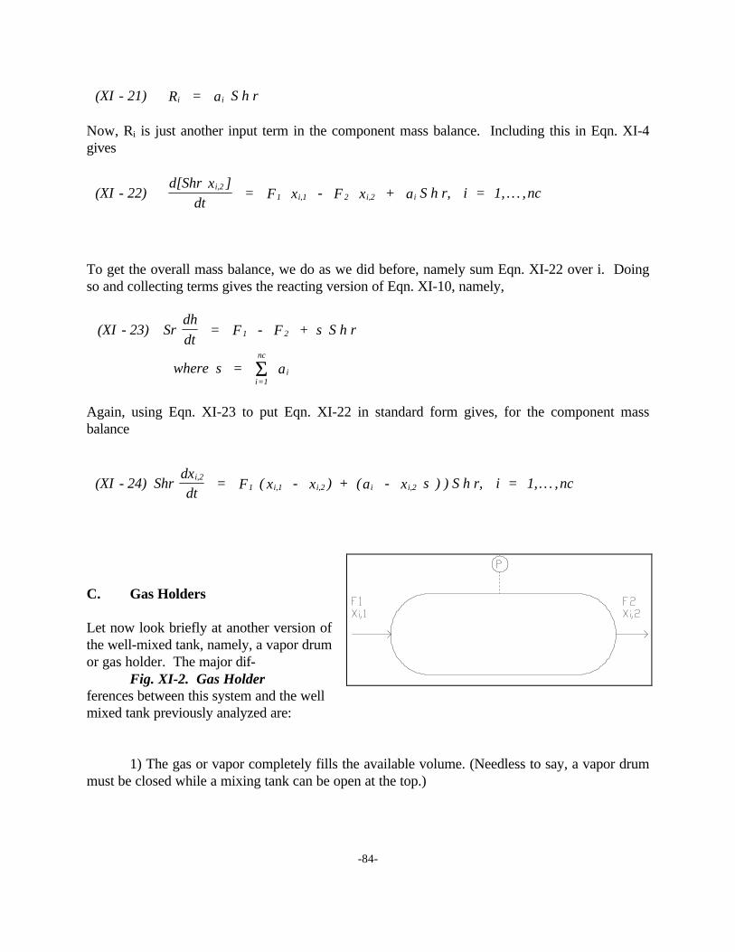
-84-

Now, Ri is just another input term in the component mass balance. Including this in Eqn. XI-4gives

To get the overall mass balance, we do as we did before, namely sum Eqn. XI-22 over i. Doingso and collecting terms gives the reacting version of Eqn. XI-10, namely,

Again, using Eqn. XI-23 to put Eqn. XI-22 in standard form gives, for the component massbalance

C. Gas Holders

Let now look briefly at another version ofthe well-mixed tank, namely, a vapor drumor gas holder. The major dif-

Fig. XI-2. Gas Holderferences between this system and the wellmixed tank previously analyzed are:

1) The gas or vapor completely fills the available volume. (Needless to say, a vapor drummust be closed while a mixing tank can be open at the top.)

(XI - 21) R = a S h ri i

(XI - 22) d[Sh x ]

dt = F x - F x + a S h r, i = 1, . . . ,nc

i,21 i,1 2 i,2 i

ρ

(XI - 23) Sdh

dt = F - F + S h r

where = a

1 2

i=1

nc

i

ρ σ

σ Σ

(XI - 24) Shdxdt

= F ( x - x ) + (a - x ) ) S h r, i = 1, . . . ,nci,2

1 i,1 i,2 i i,2ρ σ

-85-

2) While assuming constant density for a liquid is not a bad first approximation, itdefinitely is for a gas.

Thus, the major the major difference between the two systems will be in variable used totrack changes in inventory. For the mixing or surge tank, it is the liquid height h. For the vapordrum it is the gas pressure P inside the drum.

Consider the vapor drum shown in Figure XI-2. Except that it must be a closed volume, itis very similar to the liquid-filled, well-mixed tank of Figure XI-1. Thus, we would expect themass balance equations to be similar and indeed they are. The only difference is in the overallmass balance. In Eqn. XI-10 (non-reacting system ) or Eqn. XI-23 (reacting system), it wasassumed that � is constant and that h varies with time. In the case of the flash drum, the situationis reversed and the overall mass balance becomes

However, ρ is not a state variable but is a function of several state variables including pressure,temperature, and composition. At the beginning of this section, we stipulated that our c-onsiderations would be limited to isothermal systems. Also, to keep the analysis within hand, letus assume that ρ is described by the ideal gas law. If a molar basis is used, then ρ is alsoindependent of composition. This leaves only pressure. Applying the chain rule of differentiationto Eqn. XI-25 gives

The ideal gas law states that ρ = P/RT. Carrying out the partial differentiation indicated in Eqn.XI-26 provides a useable form of the overall mass balance, namely,

The reader should verify that the component mass balances are the same for both the mixing tankand the gasholder.

(XI - 25) Shd

dt = F - F1 2

ρ

(XI - 26) Sh(P

) (dP

dt) = F - F1 2

∂∂∂∂ρ

(XI - 27) Sh

P

dP

dt = F - F1 2

ρ

-86-

XII. PROCESS SIMULATORS

-87-


Process simulators are computer programs for performing the kinds of process flowsheetcalculations described in these notes. These are of particular utility for simulating processes usingthe more accurate, rigorous unit operations models. A good process simulator offers a broadselection of such models. In addition, present day simulators have comprehensive physicalproperties systems offering a wide choice of equations of state, activity coefficient models, etc., aswell as extensive databases of physical properties data for both pure components and binarymixtures. They also have extensive capabilities for flowsheet convergence and optimization. Many also provide an elementary, though useful, equipment sizing and cost estimation capability.

The following are some commercially available process simulators.

A. Steady State

Two of the most widely used steady-state process simulators are ASPEN PLUS (AspenTechnology, Inc., Cambridge, MA) and PRO-IV (Simulation Sciences, Fullterton, CA). Both ofthese programs offer a large variety of unit operations models, a substantial physical propertiessystem and database, and robust methods for flowsheet convergence and optimization. ASPENPLUS also provides a conceptual level equipment sizing and cost estimation capability.

Hyprotech and COADE also offer steady-state simulators particularly suited for use onhigh-end desktop computers. Aspen Technology also provides desktop capability.

B. Dynamic

For many years about the only dynamic simulator that was readily available was DYFLOdeveloped by Roger Franks of DuPont. It is still used in many quarters as attested to by the factthat Franks's book, originally published in 1972, is still in print. DYFLO, while quite useful,requires considerable effort and skill on the part of the user.

Dynamic process simulators of reasonable reliability are just beginning to becomecommercially available. One is SPEEDUP that was originally developed by Roger Sargent andJohn Perkins at Imperial College and is now offered commercially by Aspen Technology. Another is OTIS which is currently be commercialized by Simulation Sciences. Hyprotech hasrecently come to the market with HYSIS. The leading academic dynamic simulators areASCEND (developed by A. Westerberg and colleagues at Carnegie-Mellon) and DIVA(developed by E. Gilles and colleagues at the University of Stuttgart). Another, more recent,simulator that originated at Imperial College but is now commercially available is gPROMS.

-88-

The use of real-time dynamic simulators for personnel training has grown considerably inrecent years. Several companies, such as ABB Simcon, offer a complete of services in this areafrom process modeling to development of a set of training exercises for use with the simulator.

Dynamic simulation is undergoing rapid development. Its use for both engineeringsimulation and personnel training has lead to a demand for simulators that are easy to use and thatcan provide realistic simulations of real processes. Heretofore, the development of dynamicsimulator models has been a time-consuming and error-prone activity. The most recent trend isthe development of modeling environments that allow the user to configure new equipmentmodels with a minimum of effort. Two such systems are MODEL.LA developed byStephanopoulos at MIT and ForeSee being developed at CCNY.

89

BIBLIOGRAPHY

Revised October 12, 1999Brickman, L., Mathematical Introduction to Linear Programming and Game Theory, Springer-

Verlag, New York, 1989.

Denn, M.M., Process Modeling, Longman, New York, 1986.

Douglas, J.M., Conceptual Design of Chemical Processes, Mc-Graw Hill, New York, 1988.

Felder, R., and Rousseau, Elementary Principles of Chemical Processes, 2nd ed., Wiley, NewYork, 1984.

Franks, R.G.E., Modeling and Simulation in Chemical Engineering, Wiley, New York, 1972.

Himmelblau, D., Basic Principles and Calculations in Chemical Engineering, 4th ed., PrenticeHall, Englewood Cliffs, New Jersey, 1983.

Mah, R.S.H., Chemical Process Structures and Information Flows, Butterworths, Boston, 1990.

Ostrowski, Solutions of Equations and Systems of Equations, Academic Press, New York, 1960.

Ramirez, W.F., Computational Methods for Process Simulation, Butterworths, Boston, 1989.

Reklaitis, G.V., Introduction to Material and Energy Balances,Wiley, New York, 1980.

Silebi, C.A., and Schiesser, Dynamic Modeling of Transport Process Systems, Academic Press,New York, 1992.

Westerberg, A.W., et al., Process Flowsheeting, Cambridge University Press, New York, 1979.

91

APPENDIX A. REACTION STOICHIOMETRY

October 12, 1999

The proper handling of reaction stoichiometry in material balance calculations is of theutmost importance. It must be done correctly, otherwise the calculations are at best valuelessand, if the errors are not caught, downright dangerous. The purpose here is to provide someguidelines to avoiding the most types of errors.

The recommended procedure for any reactor calculations for which a set of reactions isknown is as follows:

1) Convert any series reactions to parallel reactions.

While series reactions may be correct from the point of view of chemical kineticmechanisms, we are only interested here in getting the material balance bookkeeping straight. This is more readily done if all the reactions are in parallel form.

2) Divide all reactions through by the stoichiometric coefficient of the key component(s)

Conversion and selectivity are based on one or more key components. The correctinterpretation of these is easier if all the key components have a stoichiometric coefficient of -1. For most simple reaction systems there will only be one key component. However, there aremore complex systems for which there may be more than one key component. This will dependon the reaction chemistry and the conversion and selectivity definitions. Note that each reactioncan have only one key component.

3) Convert all reaction system performance specifications to a molar basis

Reactor performance specifications are generally made on a weight basis, e.g., (1) converta specified number of pounds of a key raw material to products and byproducts or (2) produce agiven number of kilograms of a specified product. Although raw materials are bought andproduct sold by weight, reactions take place in mols.

4) Calculate the extents of reaction of all key components first

Since the selectivity structure is based on the extents of reaction of the key components,these should obviously be calculated first. This is straightforward since in 2) we have insured thatall key components have unity stoichiometric coefficients.

5) Calculate the extents of reaction of all other components based on their stoichiometriccoefficients and the selectivity structure

92

Keep in mind that the selectivity of a key component to a particular product or byproductis the ratio of the mols of the key component converted to the target product or byproduct to thetotals mols of key component converted via all applicable reactions.

6) Calculate the stream summary for both the reactor feed and the effluent

Do this on both a molar and a weight basis.

7) Check the overall and conserved species balances

Do pounds in equal pounds out? This is a simple check if the calculations have been doneby spreadsheet. If there is a significant error, something has done wrong in the calculations. If itis small, the error probably stems from not using consistent molecular weights. (Note: Themolecular weights given in Perry's Handbook are not consistent due to round-off.) The conservedspecies balances are most readily checked on a molar basis.

93

APPENDIX B. EVALUATION OF EQUIPMENT MODEL PARAMETERS

October 12, 1999

In order to utilize the linear material balance technique, one must be able to estimatereasonable values for all the equipment model parameters. Let us look at the parameters requiredfor each of the four models described in Chapter IV:

1) Mixer (MIX)

No parameters are required for this model.

2) Reactor (REACT)

We require ∆i (extent of reaction) for each component. This is generally known in one ofthree ways:

a. The rate of each reaction rj is specified in, say, kmol/hr.

Then extent of reaction of the ith component is given by

b. The conversion Ck and selectivities Skj for each of a set of key components are specified.

Then, for the kth key component, its extent of reaction is given by

For the other components in the reaction set assigned to the kth key component

3) Separator (SEPAR)

SEPAR can be applied directly to simple separators such as a flash drum or simpledistillation column. For more complex separators (more than one feed or more than two outputstreams), an appropriate model will have to be developed as demonstrated in Appendix C. ForSEPAR we require sI for each component in the feed to the separator.

( )B aijj

nrri j−− ==

==∑∑1

1∆

( ) ,B C fk k in k−− == −−2 ∆

( ) , ,B S ai k j i j k−− == −−3 ∆ ∆

94

Most separators in use in large-scale continuous plants work on the principle of theequilibrium stage. The physical quantity that best characterizes the performance of this type ofequipment is the relative volatility. Thus, before beginning a material balance model, one shouldestimate the relative volatilities of the components involved. These estimates do not have to behighly accurate. What one want to know is the ranking of the components by relative volatilityand a reasonable estimate of the numerical values, particularly if any of these are less than, say,1.2.

a. Flash Drum

If the feed to the flash drum consists of a number of components with very high relativevolatilities compared to the others, then one can assume that these components will be almostentirely in the vapor leaving the drum while the low volatility components leave almost entirely inthe liquid. Thus, sI will be approximately 1.0 for the high volatility components and 0.0 for thelow.

The most general way to specify the performance of a flash drum is to specify the fractionof the feed that is to leave as vapor. Let γ = V/F. Then we can solve the Rachford-Rice Equationfor γ. If kR is the k-value of the reference component, then we must solve

for γ. Then the component flow rates for the liquid are given by

So, if si is defined with respect to the vapor, then

b. Simple Distillation Column

In general we know the specs on the key components, either purity specs or fractionalrecovery specs. If the separation between the keys essentially complete, then a good firstapproximation is to assume that all the components lighter than the light appear in the distillatewhile all the components heavier than the heavy key leave in the bottoms.

( )( )

Bk z

ki R i

i R

−−−−++ −−

==∑∑11

10

αα γ γ

( )( )

, ,B fk

fL ii R

F i−− ==−−++ −−

21

1

γγα γ

( ) ,

,B s

ffi

L i

F i−− == −−3 1

95

If there are components whose volatilities are intermediate between the key componentsor the separation between the keys is only partially complete, then we can estimate the distributionof the key components using the Fenske Equation.

1) Calculate Nmin based on the specification s of the key components.2) Choose one of the key components as the reference component. 3) Calculate the distribution of the non-key components using

where all the relative volatilities are with respect to the reference component.

4) Flow Split (FSPLIT)

The flow split parameter P is specified by the process engineer. It may be adjusted toachieve a specified flow rate or composition spec in a recycle stream.

( ) ( / ) ( / )minB d b d bi iN

R−− ==4 α

96

APPENDIX C. COMPLEX EQUIPMENT MODELS

October 13, 1999

Complex equipment models can be developed using a combination of the four basicequipment models developed in Chapter IV. We give a typical example, that for an absorber thathas two feeds: the vapor entering at the bottom and the absorption liquid entering at the top. Thisis shown in Figure C-1.

Figure C-1. Representation of an Absorber as Complex Separator

The absorber is modeled as two simple separators, S-11 for the vapor phase and S-12 for theliquid phase. The components absorbed from the vapor are added to the components notstripped from the liquid in mixer M-2. M-1 does the same for the non-absorbed vapor-phasecomponents and the stripped liquid-phase components. Evaluation of the separation coefficientsfor both phases can be done for dilute systems using the Kremser Equation. The details are givenin Appendix E.

A similar approach can be used for constructing models for other complex equipment items.

S-11 S-12

M-1

M-2

STin1

STin2

STin1 STin2

STout1

STout1

STout2 STout2

Complex Separator(Gas Absorber)

Linear ModelRepresentation

S-1

97

APPENDIX D. LINEAR MATERIAL BALANCE SPREADSHEET


The following is the spreadsheet for the Ammonia Synthesis Loop example presented in Section VII. Theupper part of the spreadsheet contains the problem input data. One column, the reactor deltas, is not input but iscomputed based on the molar flow rate of N2 in Stream 3 and the specified conversion.

The lower part of the spreadsheet is the stream summary that is shown in Section VII. Streams 1 and 2 areinput data. Each molar flow rate for Stream 3 is calculated based on the tear stream solution (Eqns. E-8 and E-10). Theother streams are then calculated sequentially based on Eqns. E-1 through E-5.

Also shown in the upper part of the spreadsheet is the mol% of Argon in Stream 3. This is calculated directlyfrom the stream summary. Every time a new value for P is entered, the entire flowsheet is recalculated including themol% of Argon. This provides the mechanism for adjusting P to achieve the design spec of 10 Mol% Argon by trial anderror.

Ammonia SynLoop 7/12/95

Example for MB Notes

Problem Data:

Comp si ai Delta MW

H2 0.999 -3.0 -648.96 2.016 Conv = 0.25

N2 0.998 -1.0 -216.32 28.014 P = 0.05

Ar 0.998 0.0 0.00 39.948

NH3 0.010 2.0 432.64 17.031 %Argon 5.216%

Stream Summary:

Comp ST1 ST3 ST4 ST6 ST7 ST8 ST9

lb-mol/hr:

H2 750.00 2632.13 1983.17 1981.19 1.98 99.06 1882.13

N2 250.00 865.28 648.96 647.66 1.30 32.38 615.28

Ar 10.00 192.68 192.68 192.29 0.39 9.61 182.68

NH3 4.15 436.79 4.37 432.42 0.22 4.15

Total mol/hr 1010.00 3694.23 3261.60 2825.51 436.09 141.28 2684.23

MWavg 8.83 10.10 11.44 10.58 17.02 10.58 10.58

Total lb/hr 8914.98 37314.01 37314.01 29893.71 7420.29 1494.69 28399.03

98

APPENDIX E. THE KREMSER MODEL OF GAS ABSORBERS


The preliminary design of staged gas absorption systems and liquid-liquid extractors cangenerally be accomplished with a modest amount of effort using the Kremser Equation. This isparticularly the case if the components to be absorbed or extracted from a process stream are"dilute", i.e., present in the stream at relatively low concentrations. The system must also beessentially isothermal which is generally the case for liquid-liquid extractors but not always sowith gas absorbers. Also, the vapor-liquid or liquid-liquid equilibrium should not be a strongfunction of composition. This requirement is satisfied for dilute solutions due to the smallconcentration range of either an absorbed or extracted component.

Consider the staged absorber shown in Figure E-1. The column contains N stages (6 areshown) that, for the moment, we will take to be 100% efficient. Vapor feed enters below thebottom tray of the column (Tray #1) and liquid absorbent enters on the top or Nth tray. Yin is themol fraction in the feed of a typical component being absorbed; Yout is the mol fraction of thatcomponent leaving the column. Similarly, Xin and Xout are the mol fractions of that componentin the liquid entering andleaving the column.

There are two cases ofinterest. For the first, therating case, we are toldhow many trays there arein the column (N), whatthe vapor and liquid feedrates (V and L) are, andwhat the inlet compositionsYin and Xin are. Theproblem is to determine theseparation performance ofthe column, i.e., what areYout and Xout? For thesecond Figure E-1. Staged Gas Absorbercase, that of design, we aretold what V, Yin, and Xin are as well as the value of Yout that the column is to achieve. Theproblem is to determine suitable values of L and N.

A. The Kremser Model

Let us start with a mass balance around the nth tray for a typical component. This gives

99

If the tray is at thermodynamic equilibrium, then

Substituting Eqn. 2 into Eqn. 1 give

In general we would also need an energy balance and an overall mass balance to complete theperformance equations for the tray. We eliminate this requirement by making some simplifyingassumptions:

a) yn << 1.0 and xn << 1.0, i.e., the feeds to the column are dilute with respect to thecomponents to be transferred from one phase to the other. Therefore there will be anegligible change in V and L from tray to tray. As a result, we have

i.e., V and L are constant from tray to tray.

b) The column is isothermal and isobaric. This means that kn does not vary from trayto tray, i.e., kn = k.

With these assumptions, Eqn. 3 becomes

Where S = Vk/L. This quantity is known as the stripping factor for the component in question.

Eqn. 5 is a difference equation. Before we can solve it, we must establish the boundaryconditions which are, for the vapor feed to the bottom of the column (n=0),

x0 = yin/k

And, for the liquid feed to the top of the column (n=N+1),

(1) V y V y L x L x = 0n 1 n 1 n n n n n 1 n−− −− ++ ++++ ++ ++ 1

(2) y = k xn n n

(3) V k x (V k + L ) x + L x = 0n 1 n 1 n 1 n n n n n 1 n+1−− −− −− ++

(4) V = V = V and L = L = Ln n 1 n n+1−−

(5) S x (S + 1) x + x = 0n n n+1−−1

100

xN+1 = xin.

To solve Eqn. 5 we assume a solution of the form

Substituting Eqn. 6 into Eqn. 5 and collecting terms gives a characteristic equation of the form

Solving Eqn. 7 for its characteristic values gives � 1 = 1 and � 2 = S. Our assumed solution (Eqn.6) now has the form

Applying the boundary conditions, solving for c1 and c2, and collecting terms gives

We are generally interested how much is absorbed, namely the difference between yout (= yN) andyin. This is given by

Now, let us define a fractional removal factor as

Rearranging Eqn. 10 gives

(6) x = c nnλ

(7) (S + 1) + S = 02λ λ−−

(8a) x = c + c or

(8b c + c S

n 1 1n

2 2n

1 2n

λ λ

) ==

(9) x = S S

S 1

y

k +

S 1

S 1 xn

N +1 n

N +1

inn

N +1 in

−−−−

−−−−

(10) y = S S 1

S 1 y +

S 1

S 1 k xout

NN +1 in

N

N +1 in

−−−−

−−−−

(11) = y y

k x yout in

in in

Φ−−−−

101

First, let us look at some limiting cases for Eqn. 10 as we let the number of trays increase toinfinity. For S < 1, we have

For S > 1, we haveWhat can we learn from these limiting cases? From Eqn. 13 we see that if we want to

reduce the amount of material in the vapor feed to zero, S must be < 1. In this case, the amountof the component in question in the vapor leaving the column will be equal to the amount inequilibrium with the liquid feed to the top of the column. If we are using a "clean" absorbent,then xin = 0 and we can theoretically have a clean vapor leaving the column. However, economicsand environmental considerations dictate that we reuse the absorbent. This means separating theabsorbed material from it and recycling it back to the absorber. Since no separation using finitemeans can be 100% complete, xin will generally not be zero.

If, instead of absorbing material from a vapor, we want to remove it from a liquid using avapor (a procedure known as stripping), then Eqn. 14 provides guidance. This shows that if wehave a clean stripping vapor (yin = 0), then we can theoretically reduce the amount of material inthe liquid leaving the column to zero. Otherwise, xout is in equilibrium with yin.

B. Absorber Design

1) Selection of Operating Conditions

The value of S can be set by the designer by adjusting any of a number of variables. Usually V is set process considerations. So if we want to enhance absorption, we must make S <1 by either making k sufficiently small or L sufficiently large. L can be made large up to a point. For a given V there is a limit on how large L can be without causing mal-operation of the column.

(12) = S 1

S 1

N

N +1Φ−−−−

(13) lim y xN

out in →→∞∞

→→ 0 + k

(14) xN

out + lim→→ ∞∞

→→iny

k0

102

k can be made small by raising the pressure and in some cases by lowering thetemperature. If the component being absorbed is subcritical and obeys Raoult's Law with respectto the absorbent, then

where P0(T) = the vapor of the absorbed component. It is obvious that k can be reduced by eitherincreasing the column operating pressure Pcol or by reducing the temperature T of the absorbent. Generally the available feed pressure will determine the column operating pressure; it is seldomeconomic to compress the feed to a higher pressure. The absorbent temperature cannot generallybe reduced below a the available cooling water temperature plus a suitable approach temperature. Otherwise refrigeration will be required which is expensive. Thus, it is clear that design of anabsorber system is requires the evaluation of alternatives and some design optimization.

2) Tray Requirements

If the absorber performance is specified, then fractional removal factor � is known andEqn. 12 can be solved for N. This gives a familiar form of the Kremser Equation

Let us examine how the choice of S affects the tray requirements as a function �. Table 1 givesand idea of the relationship.

Table 1.

Number of trays N for φ = S 0.9 0.95 0.99 0.999 0.95 7.2 13.0 34.8 76.6 0.90 6.1 10.1 22.7 43.8

(15) k = P (T)

P

0

col

(16) N =

[ 1

S 1]

S

ln

ln

φφ

−−−−

103

0.80 4.6 7.0 13.6 23.8 0.70 3.7 5.3 9.6 16.0

We see that for high fractional removals (φ > 0.99), the tray requirements are quite high for S >0.7 to 0.8. Since tray efficiencies for absorption are lower than those for distillation (25 to 40% istypical), ideal tray requirements should not exceed 15 to 25 if the column height is not to beexcessive (> 100 ft at a tray spacing of 2.0 ft.). Thus adjusting L to give S ≤ 0.8 is useful rule ofthumb for choosing a reasonable starting point for a design.

The effect of tray efficiency can also be included in the Kremser model. If we use theMurphree Vapor Phase efficiency EMV defined as

we can solve for the actual tray requirement NACTUAL and the overall column efficiency EO whichgives

where NIdeal is given by Eqn. 16. We see that the actual tray requirement is independent of � andis a function only S and EMV. The overall column efficiency EO as a function of these last twovariables is shown in Table 2.

Table 2.

EO for S = EMV 0.95 0.9 0.8 0.7 1.0 1.0 1.0 1.0 1.0 0.9 0.898 0.895 0.889 0.882 0.8 0.796 0.791 0.781 0.769 0.5 0.494 0.456 0.472 0.456 0.3 0.295 0.289 0.277 0.264

We see that there is not much difference between EMV and EO over most of this table. Themaximum error (S=0.6, EMV = 0.3) is 12%. Thus, for preliminary design, setting EO = EMV willnot introduce a significant error.

C. Absorber-Stripper Systems

(17) E = y y

k x yMVn n1

n n1

−−−−

(18) E = N

N =

[(1 E ) + S E ]

SO

ideal

actual

MV MVln

ln

−−

104

Absorbing a component from a gas stream into a liquid (mass separating agent or MSA)merely transfers a separation problem from one stream to another if our goal is to recover theabsorbed component in a relatively pure form. Even if all we want to do is throw it away or burnit, we still have the problem of dealing with the MSA. The flow rate of this stream will generallybe several times larger than the molar flow rate of the component being absorbed. If it is anexpensive solvent, we must reuse it for our absorption system to be economic. This meansseparating most of the absorbed component from it before recycling it back to the absorber. Evenif the MSA is water and relatively inexpensive, we may still have to reuse it for environmentalreasons if the material being absorbed is toxic, carcinogenic, or merely smells bad. The questionarises as to what is the most economical separation system for this task.

Figure E-2. Absorber-StripperSystem

The two most commonchoices are stripping anddistillation. Since distillation is aseparate subject, we will only consider stripper in these notes. A schematic diagram of anabsorber-stripper system is shown in Figure E-2. The absorber is similar to that shown in Fig. E-1except that the liquid stream leaving the bottom of the column goes to the stripper. A strippingvapor of flow rate VS is used to strip the component of interest from the liquid feed to thestripper.

Now, having a stripper will do little good if the concentration of the absorbate in the vaporleaving the stripper is not considerably higher than it is in the feed to the absorber. We havealready established that the absorber must be designed so that its stripping factor SA < 1. Thissets a value for L. Therefore, the first design decision for the stripper is the value of VS.

Let us assume that the Kremser model applies to the stripper as well as the absorber. Asin the case of the absorber itself, let us look at the limiting case of infinite trays. From Eqn. 14,XSout = 0 for clean stripping vapor (ySin = 0) if SS > 1. Now, if we use the same rule of thumb forSS as we do for SA, SS �1/0.8 = 1.25. Therefore S S/SA = 1.25/0.8 = 1.6.

105

This means that

Thus, for VS to be much less than VA, KS must be much greater than KA. How can this beaccomplished? Two of the most commonly used ways are by pressure swing and by thermalswing, quite often a combination of both.

Let us consider pressure swing first. Suppose that the absorber operates at a pressure of10 atm and we choose to operate the stripper at 1 atm. Then, from Eqn. 15, KS = 10 KA so VS =0.16 VA. This is an improvement but not an overwhelming one. We have only increased theconcentration of the absorbate by a factor of 6.25. It is obvious that, unless the absorber pressureis very high, stripping by pressure swing only is not very effective.

Suppose that the absorber is run at a temperature just above that of cooling water, say 30C, and that we heat the bottoms of the absorber to a much higher temperature before feeding it tothe stripper. If the absorbate is subcritical and follows Raoult's Law, we would expect asubstantial increase in K going from the absorber to the stripper. As an example, suppose we areabsorbing methanol in water and we operate the absorber at 30 C and the stripper at 85 C. ThenK in the absorber will be about 0.25 atm while that in the stripper will be about 2.0 atm, animprovement of a factor of 8.0. If we operate the stripper almost at the atmospheric boiling pointof water, then the improvement will be closer to a factor of 15.0.

If the absorber also operates at 10 atm, then the overall improvement by the combination ofpressure and temperature swing is on the order of 50 to 100 depending upon the operatingtemperature of the stripper.

Recovering the absorbate from the stripping vapor may still be a problem. If the amountof vapor is small enough, the absorbate can be recovered by condensation if that is our purpose. On the other hand, if the absorber is used for pollution control, the overhead from the stripper canbe sent directly to an incinerator to recover the heating value of the absorbate. There are manypossibilities.

It should be kept in mind that the above analysis is based on the limiting behavior ofabsorbers and strippers for infinite trays. Since the number of trays must be finite, there will besome unstripped absorbate in the bottoms of the stripper, some of which will, on recycle, appearin the overhead of the absorber (refer to Eqn. 10). The amount left in the stripper bottomsbecomes another design decision subject to optimization.

(19) V K

V K = 1.6

S S

A A

Material Balance Notes

Documents

Transcript of Material Balance Notes