Matcont Tutorial: ODE GUI version

Hil Meijer

July, 2016

‘ ‘If you want to get credit for solving a complicated mathematical problem,you will have to provide a full proof. But if you’re trying to make somethingas easy as possible, you want to make it foolproof–so simple even a fool could

couldn’t screw it up.”1

1 Introduction and Installation

This tutorial tries to explain the basics of how to use the numerical bifurcationpackage MATCONT by going through an example. This is a condensed andshort overview, i.e. not all details and philosphy are explained, and this tutorialcannot substitute a complete course. We aim at explaining how you can use thesoftware so we assume a basic knowledge of bifurcation theory. As with manypractical things one learns, you will only master it by performing the proceduresyourself. So hands on!If you want to have more precise details, then go to the matcont website onsourceforge. Here you find more elaborated tutorial sessions. You can also lookat course material of “Introduction to Numerical Bifurcation Analysis” on thewebsite of Yuri Kuznetsov, under teaching. Another reference is 2.

We try to cover the following procedures in this tutorial

• Installation, including steps on installing a compiler

• System definition and simulation

• Continuation of equilibria in one parameter

• Continuation of codim 1 bifurcations of equilibria in two parameters

• Starting Limit Cycle from a Hopf point or time simulation

• Continuation of codim 1 bifurcations of Limit Cycles

• Computing homoclinic orbits1Every one computer is different from the other. So, although these instructions have been

checked step by step, do not be surprised if your computations take a different direction. Justtry again but now in the other direction.

2New features of the software MatCont for bifurcation analysis of dynamical systems. A.Dhooge, and W. Govaerts, Yu.A. Kuznetsov, H.G.E. Meijer and B. Sautois, Mathematicaland Computer Modelling of Dynamical Systems, Vol. 14, No. 2, pp 147-175, 2008

1

1.1 Starting Matcont

1. Please let Matlab be installed, and download matcont (latest versionhttp://sourceforge.net/projects/matcont/files/matcont/matcont6p3/). Thisis the GUI-version, and should not be confused with the version for mapsor command line. Unzip the pacakge to a folder of your choice.

2. For periodic orbits we use compiled C-code to speedup the computation ofthe Jacobians. Over the years, the support of matlab for compilers hasreduced now relying on manual installation of a compiler by the user. Toovercome this we have precompiled the necessary files. You can downloadthese from http://sourceforge.net/projects/matcont/files/Auxiliaries/MEXfiles/

2a. Choose your platform mexw32, mexw64, mexmaci64. You can check thiswith “mexext” on the Matlab command line if you are not sure. Downloadthe 7 files and put them in the folder LimitCycle of your matcont folder.

2b. If for some reason, option 2a does not work you should have a compiler3. If you receive complaints about a compiler, type ‘mex -setup’ on thecommand line and choose the compiler you installed or lcc, the Matlabcompiler. Start matcont again.

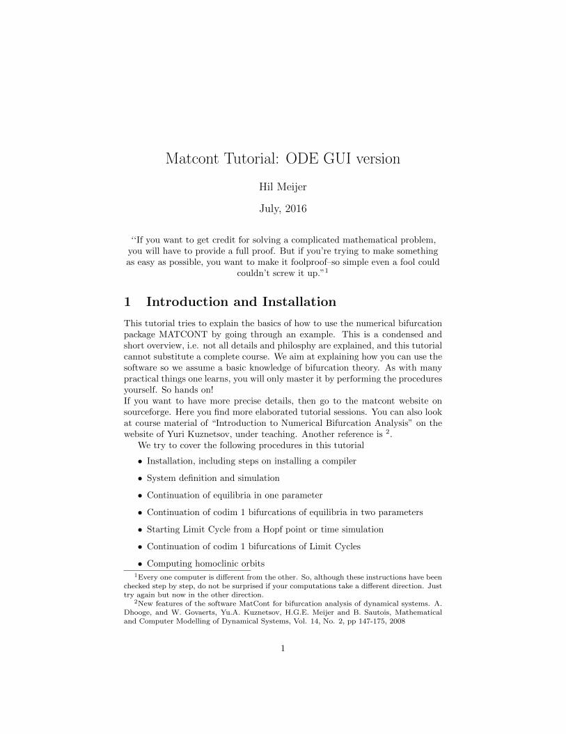
3. =⇒ Switch to the matcont directory and type ‘matcont’. Some windowsshould appear as in Figure 1. You can now start using Matcont.

Now several windows will open with a standard system called adapt2. Atypical screenshot is shown in Figure 1. One window is titled matcont andhas several menu options. For instance, to end your matcont session, choose‘Select’ in the matcont window and then ‘Exit’. Hereafter we will indicatethis with matcont:Select|Exit. Alternatively one clicks on the close button ofthe matcont window. You matlab working folder must be the matcont folder,otherwise not all windows will close. If you actually ended your session, type‘matcont’ to restart it.

3We will try to implement vectorization in the near future. For now the situation is asfollows

1. Windows XP (or Vista/7 with 32-bits processor), works fine, run mex -setup and choosethe lcc compiler.

2. Windows 7: You will need to install Visual Studio 2010 Express and SDK 7, as indicatedin http://www.mathworks.com/support/compilers/R2010b/win64.html (Windows 8&10 not tested)

3. MAC: If at mex -setup you can select gcc without problems, proceed. Otherwise youhave to install the XCode package.

4. Linux: this has its gcc compiler properly installed on most distributions.

2

Figure 1: A typical matcont startup screen

2 Equilibria in Lorenz84

In this tutorial we will first investigate some simple equilibrium bifurcationsin the Lorenz-84 model, which can be seen as a metaphor of the large-scaleatmospheric circulation, given by x′ = −y2 − z2 − ax+ aF,

y′ = xy − bxz − y +G,z′ = bxy + xz − z.

(1)

2.1 Specifying a new model

We need to tell Matcont what model we want to study. We will now go throughthis process. The result will be that a m-file is created and placed in the folderSystems of your Matcont folder. This file has the name of your system, and acall to this m-file allows Matcont to evaluate the right-hand side (RHS) of yourODE.

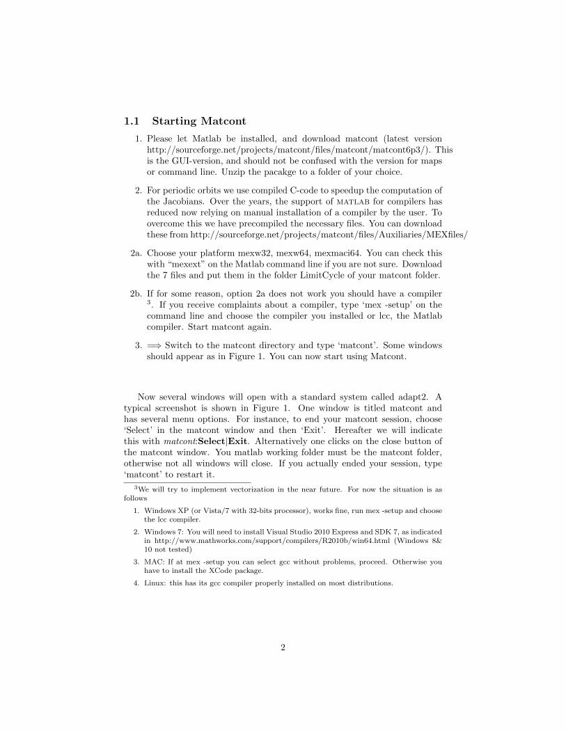
To specify the differential equations of the sytem click ‘(matcont):Select|Systems|New’and a window titled ‘System’ appears with fields ‘Name system’, ‘Coordinates’,‘Parameters’, ‘Time’, options for derivatives and a large box. The exact appear-ance of the System window depends on the operating system and the availabilityof the Matlab Symbolic Toolbox. If the latter is present, the lowest line will read

3

‘symbolically’. If possible, one should always choose to compute first, secondand third order derivatives symbolically as this is the most reliable and fastestoption 4. If you have a large system (many variables) or complex functions,it may be enough to have just first order derivatives. Computing higher orderderivatives symbolically may take too much time.

Fill the fields as follows

• Name: Lorenz84

• Coordinates: x,y,z

• Parameters: a,b,F,G

• Time: t (we do not use it here.)

• Select symbolic derivatives up to order 3 (if possible).

• In the big field specify the ODE:

x’=-y*y-z*z-a*x+a*Fy’=x*y-b*x*z-y+G

z’=b*x*y+x*z-z

To avoid typos you may also use the input from the file www.math.utwente.nl/∼meijerhge/MT.txt(or google Hil Meijer and go to my software page). Now you can copy-paste allthe required fields. You will have something like in Figure 2 and click Ok.If you want to change the system or correct the input choose ‘(matcont):Select|Systems|Edit/Load’,select the system you want to edit and press ‘Edit’.We have observed the following typical mistakes (in addition to simple typos):

• Some names (e.g. C) are internal matlab commands or variables andcannot be used.

• Do not use spaces between variables or parameters in their input fields

• Make sure that multiplication is written explicitly with * or you get errorslike ‘Unbalanced or misused parentheses or brackets’ or ‘error using ==>eval, Index exceeds matrix dimensions’.

• Specify the differential equations in the same order as the order of thecoordinates.

If you filled the fields correctly, the System window now disappears, andyou will see that the field ‘(matcont):System’ displays Lorenz84 as the currentsystem. If selected, the information field ‘(matcont):Derivatives’ shows the stringSSSNN meaning that symbolic 3rd order derivatives of the RHS will be used.

4The first and second are mostly used in the continuation, the third order is useful forcomputing normal forms accurately.

4

Figure 2: Specifying a new model

2.2 Time Simulations

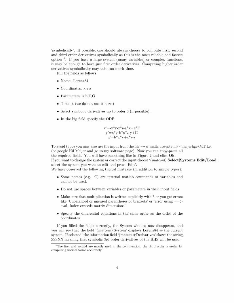
Click ‘(matcont):Type|Initial point|Point’ to initialize the computation of anorbit starting from a point. In the matcont window the curve type is now P O,every curve type has a similar meaning. Two extra windows ‘Starter’ and ‘In-tegrator’ appear. The first is to specify initial conditions and parameter values,the second to select the numerical integrator and change its settings. In thestarter window set a = .25, b = 4, F = .5, G = .5. We also want to see how theorbits look like and for this we open a window ‘(matcont):Window|Plot|2D-plot’. We want to see the x, y-plane. In the window ‘Layout|Variables onaxes’, we select x as abscissa (standard) and y as ordinate, press ‘OK’. Nowwe should adjust to the range of values that x(t) and y(t) will have. Using‘(2Dplot:1):Layout|Plotting region’, set the axes range from 0 to .5 for theabscissa and -.5 to .5 for the ordinate. In ‘Integrator’ change ‘Interval’ to 50and ‘MaxStepsize’ to 0.1.

After these preparations we are ready to compute some orbits: Select ‘(mat-cont): Compute|Forward’. Starting from (x, y, z) = (0, 0, 0) converges to(−.13444588, .359872257,−.170597270). You can monitor the orbit and its finalvalues by opening via numeric window. Select ‘(matcont): Window|Numeric’and recompute the orbit. You can try also other initial points and check thatthese also converge to this point. So we have a(n apparent) global attractor.

5

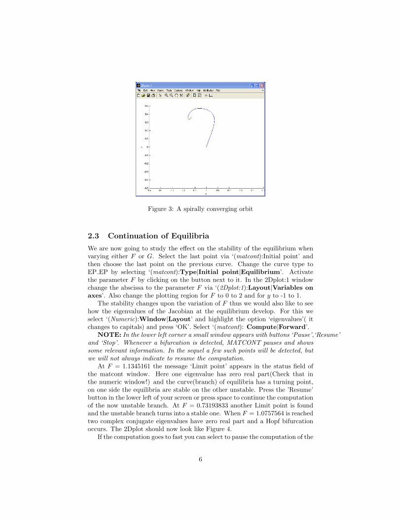
Figure 3: A spirally converging orbit

2.3 Continuation of Equilibria

We are now going to study the effect on the stability of the equilibrium whenvarying either F or G. Select the last point via ‘(matcont):Initial point’ andthen choose the last point on the previous curve. Change the curve type toEP EP by selecting ‘(matcont):Type|Initial point|Equilibrium’. Activatethe parameter F by clicking on the button next to it. In the 2Dplot:1 windowchange the abscissa to the parameter F via ‘(2Dplot:1):Layout|Variables onaxes’. Also change the plotting region for F to 0 to 2 and for y to -1 to 1.

The stability changes upon the variation of F thus we would also like to seehow the eigenvalues of the Jacobian at the equilibrium develop. For this weselect ‘(Numeric):Window|Layout’ and highlight the option ‘eigenvalues’( itchanges to capitals) and press ‘OK’. Select ‘(matcont): Compute|Forward’.

NOTE: In the lower left corner a small window appears with buttons ‘Pause’,‘Resume’and ‘Stop’. Whenever a bifurcation is detected, MATCONT pauses and showssome relevant information. In the sequel a few such points will be detected, butwe will not always indicate to resume the computation.

At F = 1.1345161 the message ‘Limit point’ appears in the status field ofthe matcont window. Here one eigenvalue has zero real part(Check that inthe numeric window!) and the curve(branch) of equilibria has a turning point,on one side the equilibria are stable on the other unstable. Press the ’Resume’button in the lower left of your screen or press space to continue the computationof the now unstable branch. At F = 0.73193833 another Limit point is foundand the unstable branch turns into a stable one. When F = 1.0757564 is reachedtwo complex conjugate eigenvalues have zero real part and a Hopf bifurcationoccurs. The 2Dplot should now look like Figure 4.

If the computation goes to fast you can select to pause the computation of the

6

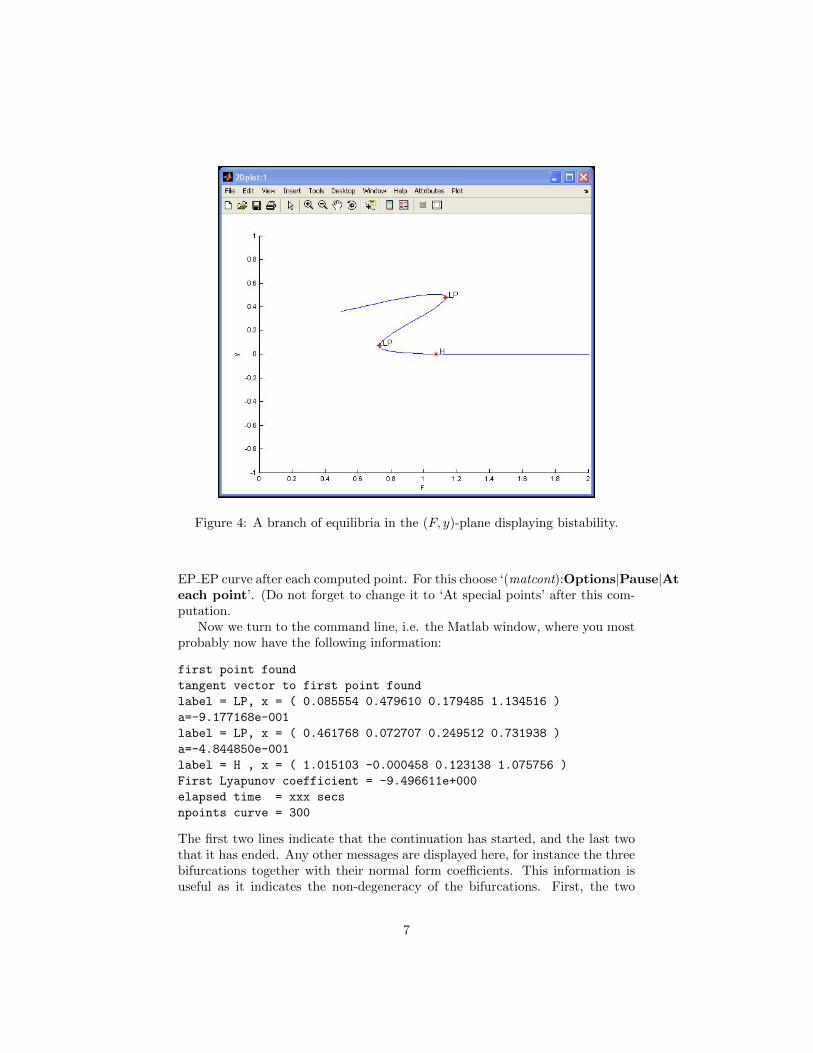
Figure 4: A branch of equilibria in the (F, y)-plane displaying bistability.

EP EP curve after each computed point. For this choose ‘(matcont):Options|Pause|Ateach point’. (Do not forget to change it to ‘At special points’ after this com-putation.

Now we turn to the command line, i.e. the Matlab window, where you mostprobably now have the following information:

first point found

tangent vector to first point found

label = LP, x = ( 0.085554 0.479610 0.179485 1.134516 )

a=-9.177168e-001

label = LP, x = ( 0.461768 0.072707 0.249512 0.731938 )

a=-4.844850e-001

label = H , x = ( 1.015103 -0.000458 0.123138 1.075756 )

First Lyapunov coefficient = -9.496611e+000

elapsed time = xxx secs

npoints curve = 300

The first two lines indicate that the continuation has started, and the last twothat it has ended. Any other messages are displayed here, for instance the threebifurcations together with their normal form coefficients. This information isuseful as it indicates the non-degeneracy of the bifurcations. First, the two

7

Limit Point bifurcations are shown, x indicates the three variabels x, y, z andthe value of the active parameter F of the bifurcation point. Then the normalform coefficients are given, note that for a Limit Point the sign of this coefficientis not unique 5. Finally, we know that the limit cycle born from the Hopfbifurcation is stable as the first Lyapunov coeffiecient is negative.

2.4 Continuation of codim 1 bifurcations of equilibria

Figure 4 showed a phenomenon called hysteresis or bistability. This is an im-portant feature of nonlinear (differential) equations. In parameter space regionsof bistability are usually delimited by a wedge of Limit Point bifurcations whichwe will compute here.

Select one of the Limit points found in the equilibrium continuation asinitial point ‘(matcont):Select|Initial point’. Activate F and G as activeparameters. Close the 3D-plot and re-open the 2D-plot. Change the ordi-nate of the 2D-plot to the parameter G and its range to 0 to 2. Now se-lect ‘(matcont):Compute|Forward’ and when finished also ‘Backward’. At(F,G) = (0.4663649, 0.2919545) a Cusp bifurcation (CP) and at (F,G) =(1.6840517, 1.6829686) a Zero-Hopf bifurcation is detected. You have now com-puted the wedge within which you have bistability.

Finally we also compute a curve of Hopf bifurcations: select a Hopf pointanalogously as for the Limit point as initial point. Change the curve type to H Hvia ‘(matcont):Type|Curve|Hopf’. Here we set F and G as active parameters.Press ‘Compute|Forward’ and ‘Compute|Backward’ to obtain the diagramas in Figure 5.

2.5 Challenge problem:

Consider the following 2D prey-predator model from mathematical ecology{x′ = rx(1− x)− fracxyx+ a,

y′ = −cy + xyx+a −

dy2

y2+b2 .

We set a = 0.6, b = c = 0.25 and also r = 2 and d = 0.1.Produce a bifurcation diagram with all Limit Point and Hopf bifurcation

curves you can find in the (r, d)-parameter plane. That is, keep a, b, c fixed anduse r and d as free parameters. You will have to specify a new system (renamec to cc), and to do all continuation of equilibria and LP and H points, just aswe discussed. The nicest solution (on Tuesday morning) will get a small prize.

5Can you understand why from the formula a = 〈p,B(q, q)〉?

8

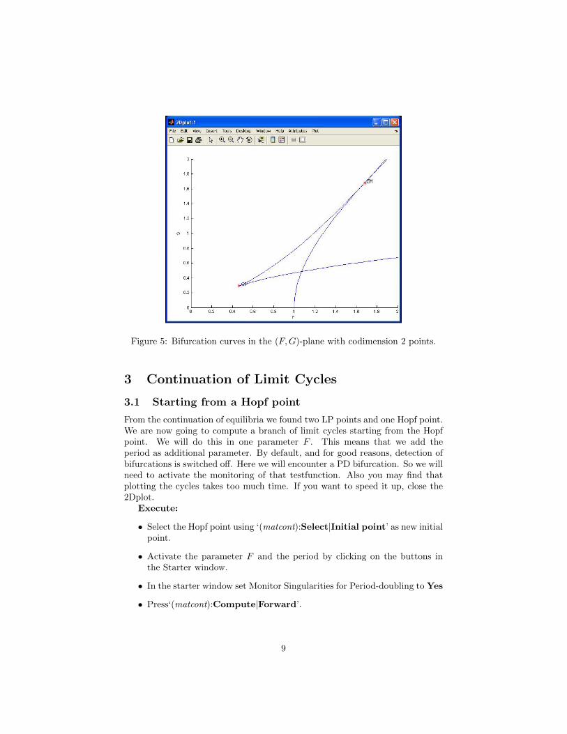
Figure 5: Bifurcation curves in the (F,G)-plane with codimension 2 points.

3 Continuation of Limit Cycles

3.1 Starting from a Hopf point

From the continuation of equilibria we found two LP points and one Hopf point.We are now going to compute a branch of limit cycles starting from the Hopfpoint. We will do this in one parameter F . This means that we add theperiod as additional parameter. By default, and for good reasons, detection ofbifurcations is switched off. Here we will encounter a PD bifurcation. So we willneed to activate the monitoring of that testfunction. Also you may find thatplotting the cycles takes too much time. If you want to speed it up, close the2Dplot.

Execute:

• Select the Hopf point using ‘(matcont):Select|Initial point’ as new initialpoint.

• Activate the parameter F and the period by clicking on the buttons inthe Starter window.

• In the starter window set Monitor Singularities for Period-doubling to Yes

• Press‘(matcont):Compute|Forward’.

9

• When a Period-Doubling bifurcation is detected at F = 7.129405 andF = 12.8991, inspect the normal form coefficient b of the Period-Doublingbifurcation on the command line.

• press ‘Resume’ and wait until it has finished.

Results To inspect the results we will use a 3D plot in phase space. Thefollowing commands should result in a figure similar to Figure 6.Open the plot with ‘(matcont):Window|Plot|3D-Plot’. Choose OX=z, OY=F ,OZ=y in the draw3 attributes window. Change the plotting the region toz, y ∈ [−2, 2], F ∈ [0, 15].

Figure 6: Equilibria and Limit cycles in (F, y, z)-space. The points and limitcycles which undergo a bifurcation are indicated with red dots.

3.2 Continuation of Cycle Bifurcations in 2 Parameters

3.2.1 Starting from a detected codim 1 bifurcation

From a PD point, we should be able to find the doubled period cycle, and alsothe original cycle still exists. This is just the continuation of a limit cycle inone parameter as we have done above. You may however see below that if yourPoint type is PD, then there are two options for the Curve type. The PD LCwould start the continuation of the double-period cycle. For the original cycleyou could just use LC as Point Type. We will compute the PD-bifurcation curvein the parameters F and G. Note that the period is automatically selected asfree parameter.

Execute:

10

• Select the PD point using ‘(matcont):Select|Initial point’ as new initialpoint.

• Set the curve type to Period-doubling and set F,G as free parameters.

• Open a Numeric window to monitor the multipliers along the whole curve.

• Press ‘(matcont):Compute|Forward’ and ‘(matcont):Compute|Backward’.

Results: You can now open a 2D-plot with F,G on the axes. Make sure thatthe plotting region for F is [0,15]. Select Layout|Redraw diagram. You willnow see the LP, H and PD curve. The result will start to resemble Figure 8. Onone part of the PD curve you have encountered a R2 bifurcation, i.e. a doublemultiplier -1. From this point, there is always a Neimark-Sacker bifurcation.That is missing and it is part of the next item.

3.3 Starting from a codim 2 point

Now we have also the option to start a special bifurcation curve from the Zero-Hopf point straightaway. The ZH-point has codimension two and a codimension1 Neimark-Sacker emanates here for this case.

Execute:

• Select the ZH point as initial point and Curve|Neimark-Sacker.

• Now check that F and G are the two free parameters, and select to detectR4,R3,R2 along the curve.

• In the Continuer window set MaxStepsize to 0.3 and Press Compute|Forward.

Results: If you have the 2D-plot of the previous item still open, you will seethat there is now a Neimark-Sacker bifurcation curve starting from the ZH-pointall the way to the R2-point.

Note that this procedure saves a lot of time! We start directly from thecodim 2 point, without any intermediate steps with Limit Cycles. It is knownnot to work if the bifurcating periodic orbit changes direction quickly or whenthe normal form coefficients are very small or very large. Then one has tocompute the bifurcation point with higher accuracy, use symbolic derivativesand play with the amplitude see 6.

3.4 Visualizing your output

So far, we have already plotted some of the continuation results. It is alsopossible to load the output and plot and manipulate it yourself. We will givea nontrivial example of plotting the profile. This is nontrivial as the data isstored in a condensed way. So we will discuss what data we have and then cometo the command line commands.

6Yu.A. Kuznetsov, H.G.E. Meijer, W. Govaerts and B. Sautois, Switching to nonhyperboliccycles from codim 2 bifurcations of equilibria in ODEs, Physica D 237 No. 23 (2008) 3061-3068

11

Suppose we know how many mesh-points were used. This can be determinedfrom the f variable, simply look up the first entry equal to 1. Now we need

• the index of the periodic orbit we want to plot: say ii.

• the profile of one variable, say the jj-th: x(jj:ndim:end-2,ii)

• the time-mesh tau=f(1:ntst+1,ii), with 0 = τ0 < τ1 < ... < τntst = 1.

• the period T= x(end-1,ii) to scale the mesh back from [0,1] to [0,T]

So we could try to plot:

ntst=20;ii=4;jj=1;ndim=3;

plot(f(1:ntst+1,ii)*x(end-1,ii),x(jj:ndim:end-2,ii))

You will get an error message because the computed curve x contains also dataabout the orbit at the fine mesh-points, while you are trying to plot the profileonly at the coarse mesh-points. A first correction would be to plot only thecoarse grid:

ntst=20;ii=250;jj=1;ndim=3;ncol=4;

plot(f(1:ntst+1,ii)*x(end-1,ii),x(jj:ndim*ncol:end-2,ii))

This is usually not good enough, so we actually want the detailed grid. For thiswe need to know that between to mesh-points the orbit is stored at equi-distanttime-points ti,j = ti + j

m (τi+1−τ), j = 0, 1, ...,m. The following are the correctcommands.

Execute:

load Systems\Lorenz84\diagram\H_LC(1).mat

ii=240;jj=1;ndim=3;ntst=20;ncol=4;

mesh=sort([reshape(repmat(f(1:ntst,ii),1,ncol)+...

repmat((0:ncol-1)/ncol,ntst,1).*repmat(diff(f(1:ntst+1,ii)),1,ncol),ntst*ncol,1); 1]);

plot(mesh*x(end-1,ii),x(jj:ndim:end-2,ii))

Results: You

4 Connecting Orbits

In the following instructions we will see how to start the computation of homo-clinic orbits. The main difficulty is to get good starting data for the continua-tion. We will show two methods that may be useful to accomplish this.

4.1 Homoclinic orbits starting from a limit cycle

Sometimes when following a limit cycle you will notice that the parameters donot change anymore. Meanwhile the period goes to infinity. Typically, in agraphic window plotting the continuation parameter versus the period you see

12

something as in Figure 7right. In such cases you may suspect that you areclose to a connecting orbit. You will have to look at the orbit to be sure. Butsuppose you notice that the orbit is close to a steady state at some point. Thenit would be nice to take this as starting data for the computation of a connectingorbit. This method is implemented in Matcont, for homoclinic orbits only. Thealgorithm checkes when the orbit first gets closest to the initial point. Thisassumes that we start from a limit cycle. Along a limit cycle we can make aguess for an equilibrium by checking at which point of the cycle the vectorfieldhas smallest norm. This goes well for a single equilibrium, but not for two.To have a good starting limit cycle we first do a simulation. The limit cyclewe get from starting at the Hopf bifurcation does not get close to a homoclinicbifurcation. So we have to find another.

Execute (Time Simulation)

• Set Type|Initial Point|Point and in the Starter window set x = .1, y =1, z = .3 and F = 3, G = .8.

• In the Integrator window set Interval to 50. Open a Window|2D graphicwith x between 0 and 2 and y between -1.5 and +1.5.

• If you Compute|Forward you will get something like Figure 7left.

• Now via the main window Select|Initial Point the last point of the orbityou just computed.

• Change the interval in the Integrator window to 10 (roughly one period)and Compute|Forward.

• Intermediate Result 1 If you redraw the curve in the 2Dplot (In the 2Dplotwindow there is an option Plot|Clear/Redraw curve), it looks like wehave an interesting limit cycle.

Execute (Starting Limit Cycle Continuation from a Simulation):

• In the Starter window press Select Cycle and change the number oftest intervals to 40. Select the Period and G as free parameters (tickthe boxes) and in the Continuer window set MaxStepsize to 1.0. Open anumeric window and check that the parameters and Period are displayed.

• Press Compute|Backward and during the continuation observe that Gfirst goes up and settles toGfinal = 1.018893. If not, select Compute|Forward.You can zoom in (where?!) to see that the limit cycle might be close to asaddle-focus.

• Intermediate Result 3 At the end of the continuation, change the variablesin the 2Dplot via Layout|Variables on axes to G and Period for theabscissa and ordinate, respectively, and change Layout|Plotting regionthe range to [0.5, 1.5]× [0, 100] to obtain Figure 7.

Execute (Starting Limit Cycle Continuation from a Simulation):

13

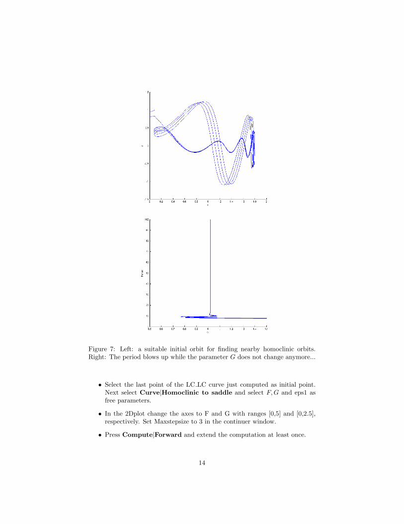
Figure 7: Left: a suitable initial orbit for finding nearby homoclinic orbits.Right: The period blows up while the parameter G does not change anymore...

• Select the last point of the LC LC curve just computed as initial point.Next select Curve|Homoclinic to saddle and select F,G and eps1 asfree parameters.

• In the 2Dplot change the axes to F and G with ranges [0,5] and [0,2.5],respectively. Set Maxstepsize to 3 in the continuer window.

• Press Compute|Forward and extend the computation at least once.

14

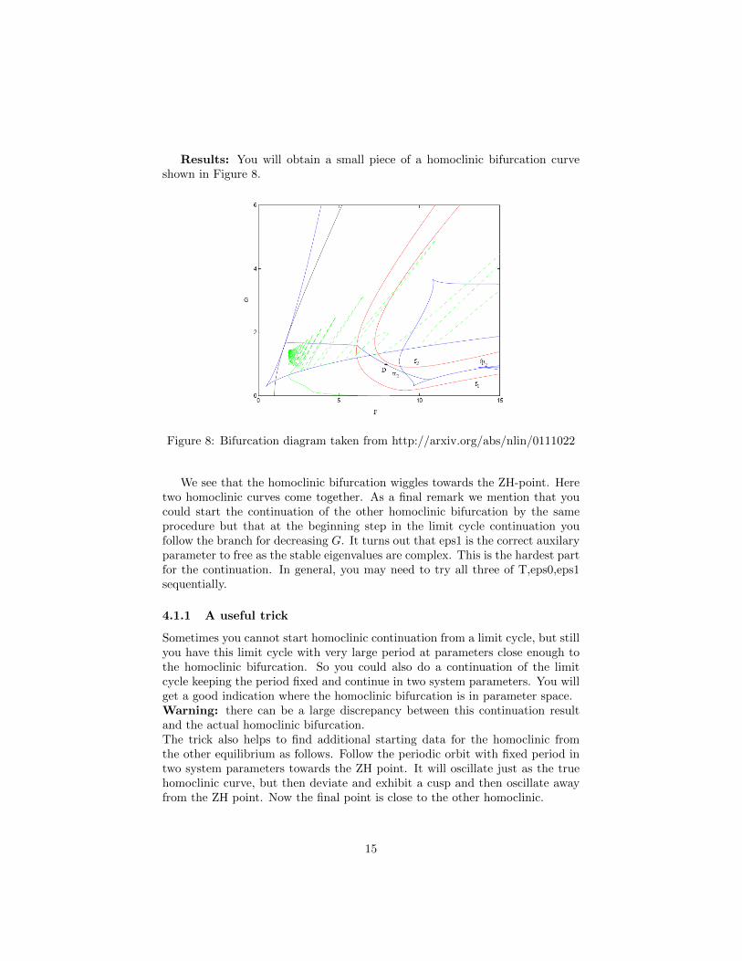
Results: You will obtain a small piece of a homoclinic bifurcation curveshown in Figure 8.

Figure 8: Bifurcation diagram taken from http://arxiv.org/abs/nlin/0111022

We see that the homoclinic bifurcation wiggles towards the ZH-point. Heretwo homoclinic curves come together. As a final remark we mention that youcould start the continuation of the other homoclinic bifurcation by the sameprocedure but that at the beginning step in the limit cycle continuation youfollow the branch for decreasing G. It turns out that eps1 is the correct auxilaryparameter to free as the stable eigenvalues are complex. This is the hardest partfor the continuation. In general, you may need to try all three of T,eps0,eps1sequentially.

4.1.1 A useful trick

Sometimes you cannot start homoclinic continuation from a limit cycle, but stillyou have this limit cycle with very large period at parameters close enough tothe homoclinic bifurcation. So you could also do a continuation of the limitcycle keeping the period fixed and continue in two system parameters. You willget a good indication where the homoclinic bifurcation is in parameter space.Warning: there can be a large discrepancy between this continuation resultand the actual homoclinic bifurcation.The trick also helps to find additional starting data for the homoclinic fromthe other equilibrium as follows. Follow the periodic orbit with fixed period intwo system parameters towards the ZH point. It will oscillate just as the truehomoclinic curve, but then deviate and exhibit a cusp and then oscillate awayfrom the ZH point. Now the final point is close to the other homoclinic.

15

4.2 Connecting orbits by homotopy

Execute:

• Set Initial Point|Equilibrium and select Curve|ConnectionSaddle. A newstarter window with more fields below the parameters and the Integratorwindows appears.

• In the Starter Window, enter x = 0.394282, y = 0.424435, z = 1.105117for the saddle at F = 6, G = 2. Set UParam=1, eps0=.001.

• In the Integrator Window set Interval to 5.

• Open a 2D-plot with x and y on the axis. Press Compute|Forward. Youwill see an orbit that departs from the saddle along the unstable manifold.Then it makes a few turns, and seems to return.

• Press ’Select Connection’. A window appears with specifications for thediscretization. These settings are fine, and press ”OK”. A new Starterwindow appears with parameters UParam1, SParam1. SParam1 indicateshow far away the trajectory is from lying within the stable manifold. Wealso see T (half the integration time), and eps1 which is the distance tothe saddle.

• Set G as an active parameter, and also SParam1 and eps1. Also open anumeric window, if you have not one open yet. Press Compute|Forward.In the 2D-plot you will see the continuation of the orbit piece. In thenumeric window you will see that SParam1 goes to zero.

• Select the special HTHOM point as Initial point (matcont:Select|Initialpoint. Now set G,T, eps1 as active parameters and set MaxStepsize to 1.Compute|Forward.

• This will take a while. You will see in the 2D-plot that the orbit piece ischanging a lot during continuation, while in the meantime the parametersF, T, eps1 are changing. But especially T is increasing as we should getcloser to the saddle and this requires a longer time for the orbit piece.

• Finally you will obtain the message that eps1 is small enough. Stop thecontinuation. Select this last point as initial point, and set the Curve Typeto ”Homoclinic Saddle”. Now you can do continuation in parameters Fand G, with eps1 as additional free parameter as before.

Another good tutorial for the initialization by homotopy for connecting or-bits, LAB5, is written by Yuri Kuznetsov. See his website or at sourceforgesee lab5.pdf in files–matcont–matcont3p3. This is for travelling waves of theFitzhugh-Nagumo equation, and very

16

4.3 Challenge problem

Study the bifurcations of Limit Cycles in the prey-predator system in §2.4. Alsoadd homoclinic bifurcation curves to your diagram.

5 Bifurcations in a periodically forced system

To make this really motivating we look at a periodically forced system, the SEIRmodel from epidemiology. The parameter β varies periodically, but we make itautonomous as follows:

S′ = µ− µS − βSIE′ = βSI − (µ+ α)EI ′ = αE − (µ+ γ)Ix′ = −2πy + x(1− x2 − y2)y′ = 2πx+ y(1− x2 − y2)

(2)

with β = β0(1 + δ cos(2πt)) = β0(1 + δx) and R = 1− S − E − I. Note that ifyou start with x, y 6= 0, then there it is not possible to find a Hopf point fromwhich you can start the continuation of a Limit Cycle.

In the main matcont window: Select|System|New and enter all fields forthe SEIR model. Note that you will be working with an equivalent system(s = logS) for numerical stability. Select symbolic derivatives of order 1 and 2.Press ok.

We will start by integrating to observe periodic dynamics. Press matcont:Type|Pointand a starter and integrator window will appear. We specify initial values in thestarter window: ss=-3,ee=-3,ii=-3,x=1,y=0 alpha=35.482,beta=5000,gamma=100,delta=.2,mu=.02,omega=6.28.The system is still sensitive so you may have to decrease MaxStepSize to .01in the integrator window. Also increase the Interval (integration time) to 20.Open a graphic window with matcont:Window|Graphic|2Dplot. Select thevariables ss and ee on the axes. Adjust the Layout|Plotting region to −10for both axes. Press matcont:Compute|Forward. You will see that after someinitial excursions it will settle to a periodic orbit.

You could inspect the x, y-dynamics by changing abscissa and ordinate viaLayout|variables on axes to see a circle.

At the bottom of the starter window we see a tempting button Select Cycle.We cannot yet push it. What the algorithm does is to find the point of thetrajectory nearest to the initial value. If it finds one, it takes that the timebetween these points as the period and fits a mesh to the computed solution.We proceed as follows: matcont:Select|Initial point and select the last point onthe curve we have just computed. In integrator window change the interval to 1and press matcont:Compute|Forward. Select Plot|Clear and Plot|Redrawcurve to see that it is a periodic orbit.

17

Now press the Select Cycle button in the starter window. A popup willappear with two fields: ”Tolerance” equal to 1e-2 and ”test intervals” equal to20. Change test intervals to 40 and press OK. Tick the boxes for beta0 andomega as free parameters in the new starter window and select ”yes” for Period-doubling under the heading monitor singularities. Change MaxStepsize to 5in the Continuer window. Open a Window|Numeric window and close thefigure. Press matcont:Compute|Forward.

If everything went well, you found two period-doubling bifurcations. Noteas well in the Numeric window that omega is now really equal to 2π. Selectone of them as initial point. Change Type|Curve to Perioddoubling and selectbeta0 and delta as free parameters.

18