ATOMIC STRUCTURES

1. Development of the concept of the atom

When the Greek Philosophers were engaged in the study of divisibility of matter, they hit upon the idea of the atom. The concept of continuity and atomicity first made their appearances in the course of the speculations of Greek Philosophers nearly 2,500 years ago. Continuity implies infinite divisibility without encountering any change in nature, such as granularity. Atomicity on the contrary implies a limitations in the process of infinite divisibility. This limit, beyond which a further division without encountering a drastic change in the nature of the substance under scrutiny, gave rise to the concept of the discrete entities of matter, the atom. According to our present evidence only the time and space appear to be infinitely divisible.

Although atomicity was given an experimental foundation only about 200 years ago, Greek Philosophers Leucipous, Demovitus and Epicurus living during the first half millenium before Chirst described the atomic concept on the basis of speculation.

The most basic and large-scale observations supporting the atomicity of matter were those of early chemists which established the definite proportions in which the chemical elements combine to yield homogeneous compounds.

2. Early Views on Atomic Structure

Speculations about the structure of the atom date from the early years of nineteenth century. In 1815 Prout proposed the hypothesis that the atoms of all the elements are composed of atoms of Hydrogen; but this view failed of acceptance when it was established that the atomic weights of some elements differ markedly from multiples of the atomic weight of hydrogen.

The discovery of electron in 1897 led to renewed interest in the internal structure of atoms by indicating that they must contain both negative electrons and positive charges.

3. Thomson Atom Model

J. J. Thomson with the above conclusions to guide him proposed the first picture of the structure of the atom. Two questions then arose :

(1) How many electrons are there in an atom ?(2) How are the electrons and the positive charges are arranged?

Using the phenomenon of X-ray scattering he came to the conclusion that the number of electrons in an atom is proportional to the atomic weight of the element.

The second point, the arrangement of electrons was not easy to resolve. Thomson had no experimental data to guide him. But since the atom as a whole was

stable, he argued that the electrons must be held by the positive charges by electrostatic forces. He further made the assumption that the positive charges were uniformly distributed in a sphere of atomic dimensions and the electrons were distributed so as to the produce a balance between the mutual repulsions of the electrons and the electrostatic force of attractions. He showed that in an atom with a single electron, the electron must be situated at the centre of the positive sphere. In an atom with two electrons, like the helium atom, the two electrons must be symmetrically situated on opposite sides of the centre at a distance equal to the radius of the positive sphere. Proceeding in this way he was able to arrange upto 100 electrons inside the positive sphere.

With this model he was able to explain the observed spectrum of elements and to some extent their origin. The difficulty was that according to this theory, hydrogen could give rise to only one spectral line. This contradicted the observed facts of several series and several spectral lines in each series. Thus, although, Thomson’s model could meet the requirements of stability and the demands of the electromagnetic theory of radiation., it lacked the experimental support. In addition to this, the conclusions of the Rutherford’s experiments of scattering of -particles completely put to rest the Thomson’s model of the atom.

4. Present Concept of the Atom

Rutherford’s experiments of scattering of -particles led to the present concept of the atom. To put it succinctly, the atom consists of

(i) a central positive nucleus wherein the individuality of the atom resides and practically whole of the mass of the atom is concentrated and

(ii) negative electrons revolving around the nucleus. Configurations of the electrons are responsible for the observed chemical and physical properties of elements.

5. Rutherford’s Model : Scattering of -particles by Atom

Before we discuss the Rutherford’s model it is necessary to describe the phenomenon of scattering of -particles by atoms. The -rays from radioactive materials had been shown to be helium atoms which have lost two electrons. The -particles whose initial velocity is of the order of 2 107 m/s, could be studied by means of the flashes of light, or scintillations, they produce on striking a zinc sulphide screen, the impact of a single particle producing a visible flash, which is readily observed under low power microscope.

If a stream of -particles, limited by suitable diaphragms to a narrow pencil, be allowed to strike a zinc sulphide screen placed at right angles to the path of the particles, scintillations occur over a well defined circular area equal to the cross section of the pencil. If now, thin film of matter, such as gold or silver foil, is interposed in the path of the rays, it is found that they pass quite readily through the foil but that area over

which scintillation occur becomes larger and losses its definite boundary, indicating that some of the particles have been deflected from their original direction.

Quantitatively, it is easy to explain the origin of the forces which causes the deflection of the -particles. The particle itself has two fold positive charge. The atom of the scattering material contain charges, both positive and negative. In its passage through the scattering material, the particle experiences electrostatic forces the magnitude and direction of which depend on how near the particle happens to approach to the centers of the atoms past which or through which it moves.

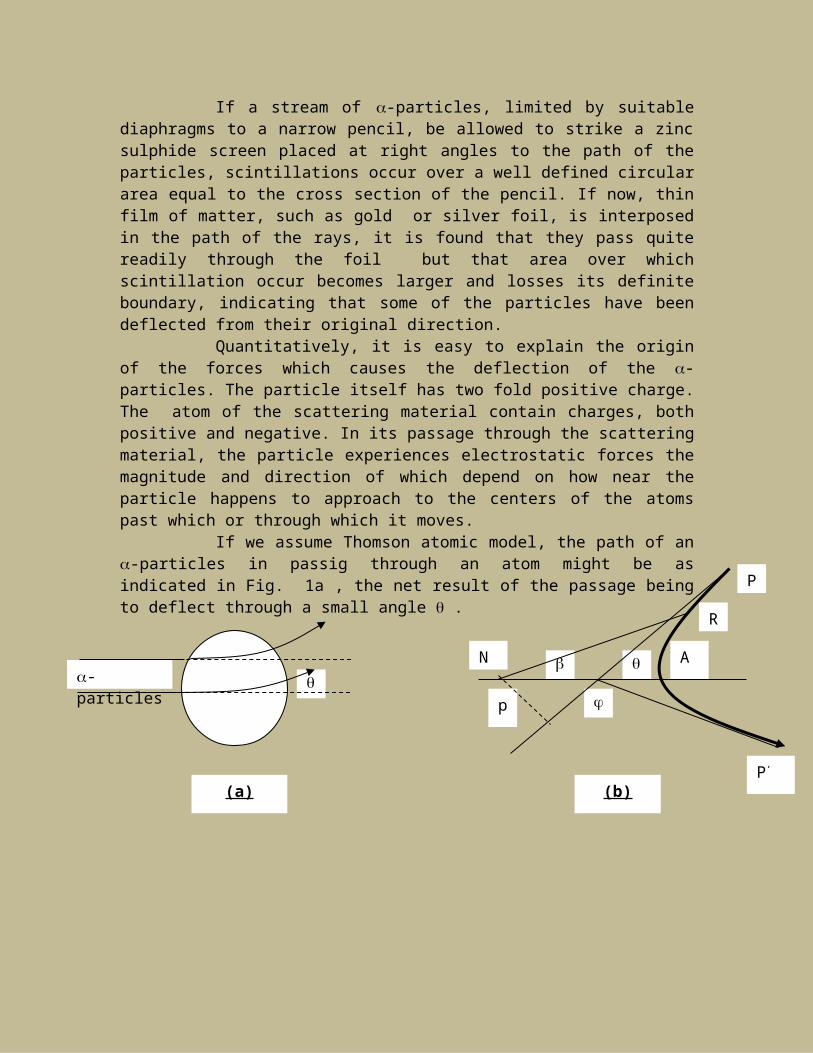
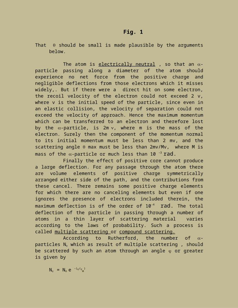
If we assume Thomson atomic model, the path of an -particles in passig through an atom might be as indicated in Fig. 1a , the net result of the passage being to deflect through a small angle .

Fig. 1

That should be small is made plausible by the arguments below.

The atom is electrically neutral , so that an -particle passing along a diameter of the atom should experience no net force from the positive charge and negligible deflections from those electrons which it misses widely,. But if there were a direct hit on some electron, the recoil velocity of the electron could not exceed 2 v, where v is the initial speed of the particle, since even in an elastic collision, the velocity of separation could not exceed the velocity of approach. Hence the maximum momentum which can be transferred to an electron and therefore lost by the -particle, is 2m, where m is the mass of the electron. Surely then the component of the momentum normal to its initial momentum must be less than 2 mv, and the scattering angle max must be less than 2mv/Mv, where M is mass of the -particle or much less than 10 –3 rad.

Finally the effect of positive core cannot produce a large deflection. For any passage through the atom there are volume elements of positive charge symmetrically arranged either side of the path, and the contributions from these cancel. There remains some positive charge elements for which there are no canceling elements but even if one ignores the presence of electrons included therein, the maximum deflection is of the order of 10-4 rad. The total deflection of the particle in passing

A

p

-particles

(a)

N

R

P

P’

(b)

through a number of atoms in a thin layer of scattering material varies according to the laws of probability. Such a process is called multiple scattering or compound scattering.

According to Rutherford, the number of -particles N which as result of multiple scattering , should be scattered by such an atom through an angle or greater is given by

N = No e -(/m

)

where No is the number of particles for = 0 and m is the average deflection after passing through the scattering material.

Discrepancies with the results from Thomson’s Model

Geiger had shown that the most probable angle of deflection of a pencil of -particles in passing through gold foil of 1/2000 mm thick is of ~ 10.

It is evident, therefore, from the above equation that the probability for scattering through angles become vanishingly small; for 300 it would be of the order of 10-12.

Geiger showed that number of particles scattered through large angle was much greater than the theory of multiple scattering predicted. In deed Geiger and Marsden showed that 1 in 8000 -particles was turned through more than 90 0 by a thin film of platinum.

These results showed that Thomson’s model could not give a correct picture of the atom.

Rutherford in 1911, proposed a new type of atomic model capable of giving to an -particle a large deflection as a result of a single encounter. He assumed that in an atom the positive charge and most of the atomic mass are concentrated in a very small region, later called the nucleus, about which the electrons are grouped in some sort of configuration (note that they are not revolving electrons).

Since normally atoms are electrically neutral, the positive charge on the nucleus must be Ze, where e is the numerical electronic charge and z is an integer, characteristics of the kind of atom.

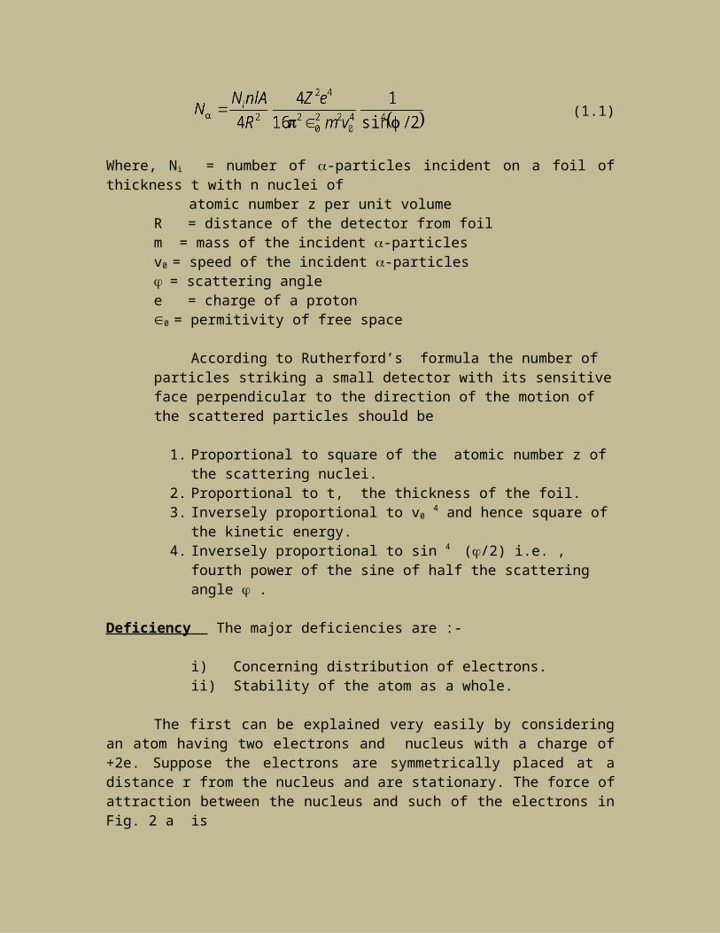
The deflection of an -particle by such a nucleus might be as illustrated in Fig. 1b. Rutherford calculated the distribution of -particles to be expected as the result of single-scattering processes by atoms of this type. According to Rutherford scattering formula, the number N of -particles reaching a small detector of area A is given by

(1.1)

Where, Ni = number of -particles incident on a foil of thickness t with n nuclei of atomic number z per unit volume

R = distance of the detector from foilm = mass of the incident -particlesv0 = speed of the incident -particles

= scattering anglee = charge of a proton0 = permitivity of free space

According to Rutherford’s formula the number of particles striking a small detector with its sensitive face perpendicular to the direction of the motion of the scattered particles should be

1. Proportional to square of the atomic number z of the scattering nuclei.2. Proportional to t, the thickness of the foil.3. Inversely proportional to v0 4 and hence square of the kinetic energy.4. Inversely proportional to sin 4  (/2) i.e. , fourth power of the sine of half

the scattering angle .

Deficiency   The major deficiencies are :-

i) Concerning distribution of electrons.ii) Stability of the atom as a whole.

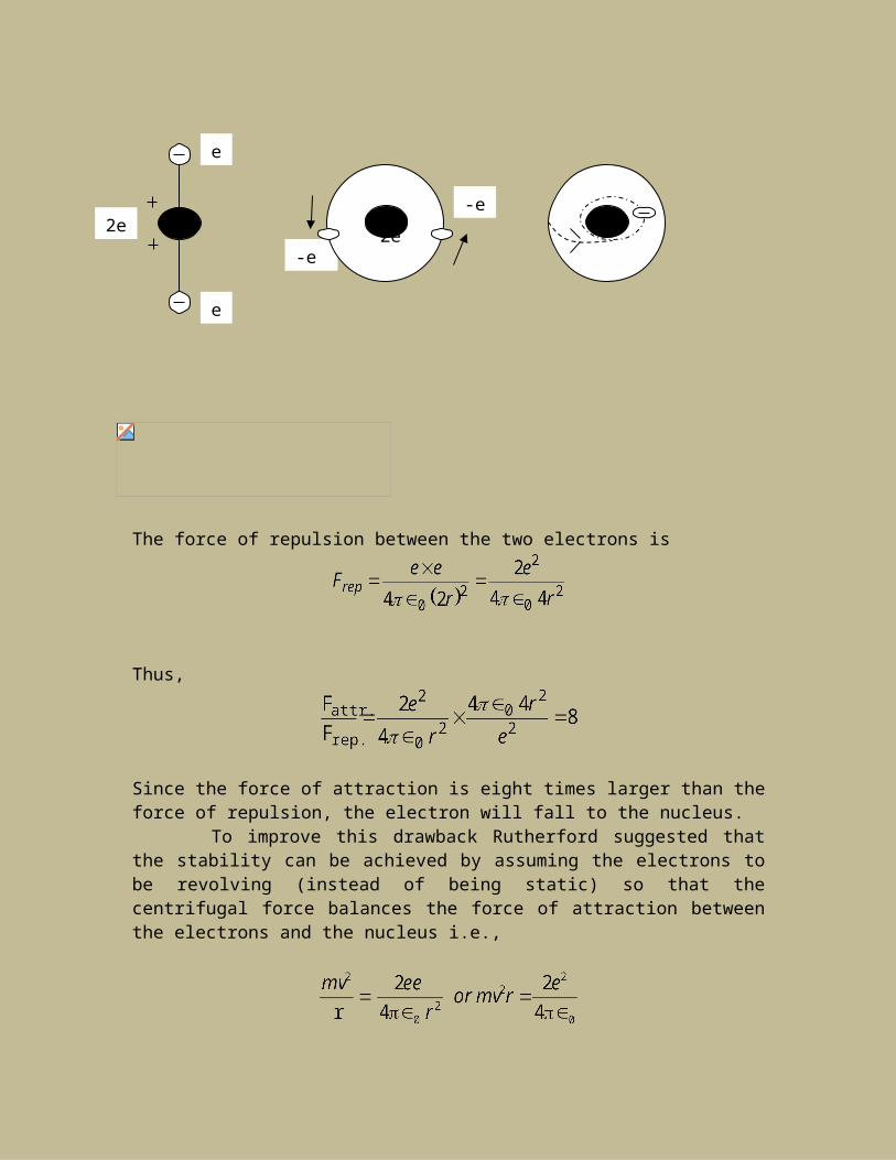
The first can be explained very easily by considering an atom having two electrons and nucleus with a charge of +2e. Suppose the electrons are symmetrically placed at a distance r from the nucleus and are stationary. The force of attraction between the nucleus and such of the electrons in Fig. 2 a is

The force of repulsion between the two electrons is

Thus,

e

-e

2e

e

2e

-e

Since the force of attraction is eight times larger than the force of repulsion, the electron will fall to the nucleus.

To improve this drawback Rutherford suggested that the stability can be achieved by assuming the electrons to be revolving (instead of being static) so that the centrifugal force balances the force of attraction between the electrons and the nucleus i.e.,

and in general

But this suggestion was confronted by the classical electromagnetic theory. According to which the electron would radiate energy. This is because the electron will have centripetal acceleration, v2/r. The system will therefore run down and the electron will approach the nucleus along a spiral path and will give out radiation of constantly increasing frequency.

v = r , = v/r

will increase as r will go on decreasing. This does not agree with the observed emission of spectral lines of fixed frequency. It was at this point that Bohr introduced his theory of structure of the atom.

6. Bohr’s Atom Model

Niels Bohr combined Rutherford’s nuclear atom with Plank’s quanta and Einstein’s photon to account for the discrepancies contained in the Rutherford’s theory.

(1) Bohr assumed that an electron in the field of nucleus was not capable of moving along every one of the paths that were possible according to classical theory but was restricted to one of a certain set of allowed paths. While it was so moving , he assumed that it did not radiate contrary to the classical theory and the energy remained constant . But he assumed that the electron could jump from one allowed path to another of lower energy and in doing so radiation was emitted containing energy equal to the difference in the energies of the two paths.

(2) As to the frequency of the emitted radiation he assumed that if Ei and Ef

are the energies of the electron when moving in its initial and final paths

respectively, the frequency of the radiation emitted is determined by the condition (1.2) where h is Plank’s constant.

(3) The third point was what determines the allowed paths, or what determines the size and shape of the orbit. He postulated that the orbit is a circle , with the nucleus as its centre. The size of the orbit is such that the angular momentum of the electron about the nucleus is an integral multiple of the natural unit h/2 which we write as .

The allowed values of the energies of the stationary states and of the spectral lines expected on the basis of Bohr’s theory are easily deduced for a system consisting of a single electron and a nucleus of charge ze as follows:

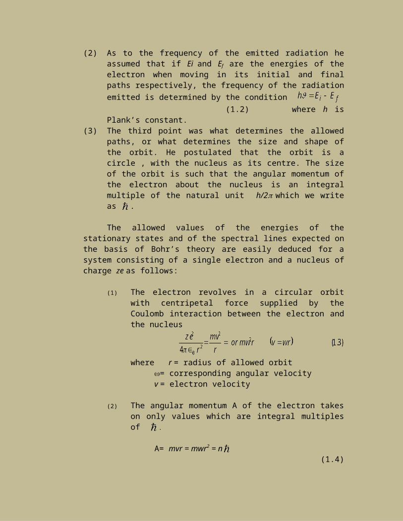
(1) The electron revolves in a circular orbit with centripetal force supplied by the Coulomb interaction between the electron and the nucleus

where r = radius of allowed orbit= corresponding angular velocityv = electron velocity

(2) The angular momentum A of the electron takes on only values which are integral multiples of .

A= mvr = mwr2 = n (1.4)

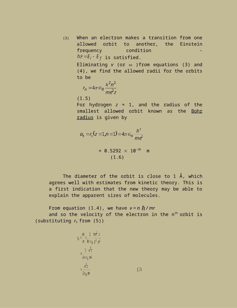
(3) When an electron makes a transition from one allowed orbit to another, the Einstein frequency condition - is satisfied.Eliminating v (or )from equations (3) and (4), we find the allowed radii for the orbits to be

(1.5)

For hydrogen z = 1, and the radius of the smallest allowed orbit known as the Bohr radius is given by

= 0.5292 10-10 m (1.6)

The diameter of the orbit is close to 1 Å, which agrees well with estimates from kinetic theory. This is a first indication that the new theory may be able to explain the apparent sizes of molecules.

From equation (1.4), we have v = n / mr and so the velocity of the electron in the nth orbit is (substituting rn from (5))

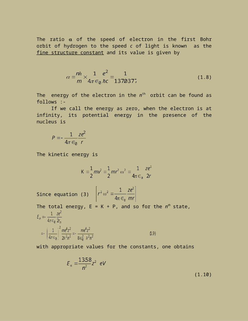
The ratio of the speed of electron in the first Bohr orbit of hydrogen to the speed c of light is known as the fine structure constant and its value is given by

(1.8)

The energy of the electron in the nth orbit can be found as follows :- If we call the energy as zero, when the electron is at infinity, its potential energy

in the presence of the nucleus is

The kinetic energy is

Since equation (3)

The total energy, E = K + P, and so for the nth state,

with appropriate values for the constants, one obtains

(1.10)

The numerical value of the negative energy of the normal state also represents the ionization energy i.e. the energy required to remove the electron.

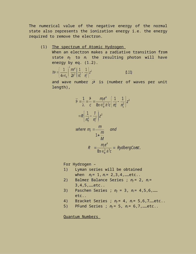
(1) The spectrum of Atomic Hydrogen When an electron makes a radiative transition from state nf to ni the resulting photon will have energy by eq. (1.2).

and wave number is (number of waves per unit length),

For Hydrogen – 1) Lyman series will be obtained

when nf = 1, ni = 2,3,4,……etc..2) Balmer Balance Series ; nf = 2, ni = 3,4,5,……etc..3) Paschen Series ; nf = 3, ni = 4,5,6,……etc..4) Bracket Series ; nf = 4, ni = 5,6,7……etc..5) PFund Series ; nf = 5, ni = 6,7,……etc..

Quantum Numbers

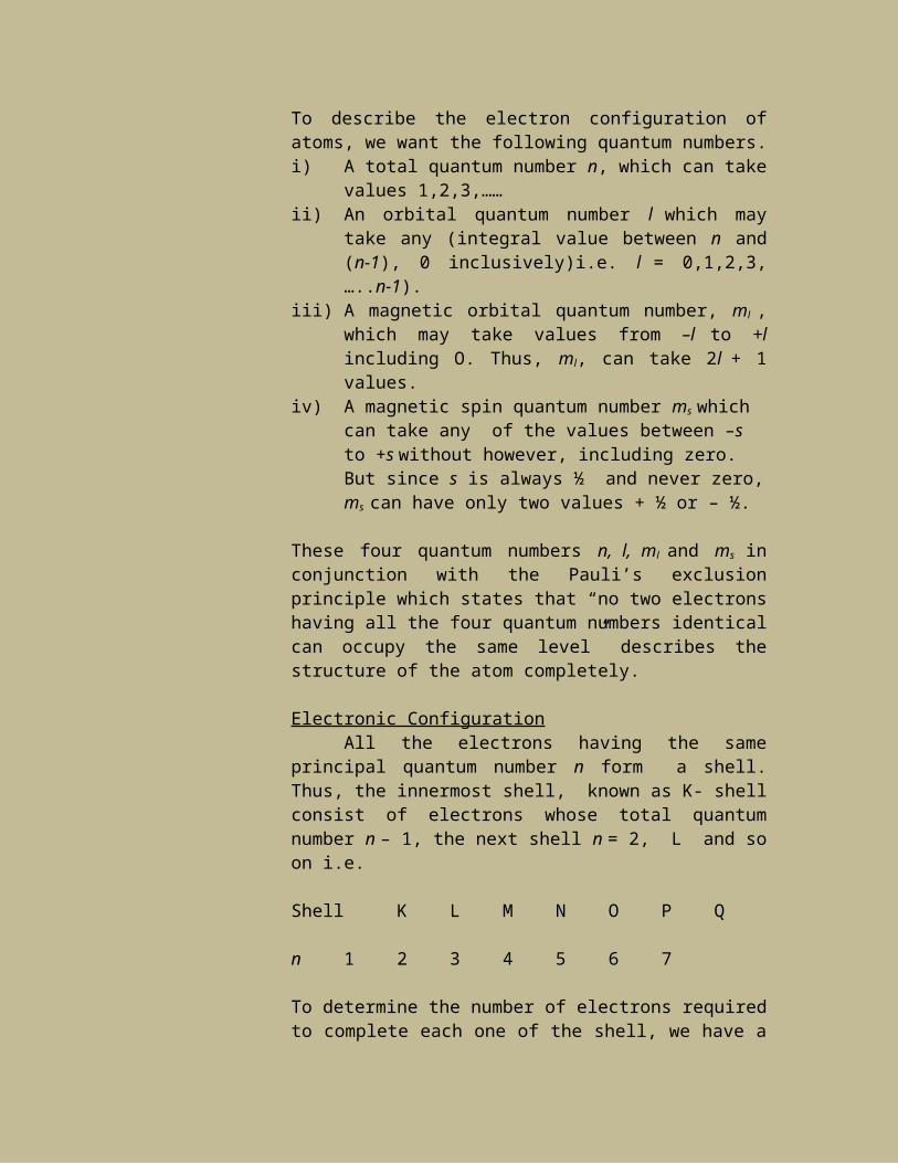
To describe the electron configuration of atoms, we want the following quantum numbers.i) A total quantum number n, which can take values 1,2,3,

……ii) An orbital quantum number l which may take any (integral

value between n and (n-1), 0 inclusively)i.e. l = 0,1,2,3,…..n-1).

iii) A magnetic orbital quantum number, ml , which may take values from –l to +l including O. Thus, ml, can take 2l + 1 values.

iv) A magnetic spin quantum number ms which can take any of the values between –s to +s without however, including zero. But since s is always ½ and never zero, ms can have only two values + ½ or – ½.

These four quantum numbers n, l, ml and ms in conjunction with the Pauli’s exclusion principle which states that “no two electrons having all the four quantum numbers identical can occupy the same level” describes the structure of the atom completely.

Electronic ConfigurationAll the electrons having the same principal quantum

number n form a shell. Thus, the innermost shell, known as K- shell consist of electrons whose total quantum number n – 1, the next shell n = 2, L and so on i.e.

Shell K L M N O P Q

n 1 2 3 4 5 6 7

To determine the number of electrons required to complete each one of the shell, we have a clue in the periodic occurrence of monatomic elements, chemically inactive, hence known as inert gases, Helium, Neon, Argon, Krypton, Xenon and Radon. Since their atomic numbers are –Helium - 2, Neon - 10, Argon - 18, Krypton - 36, Xenon - 54 and Radon – 86, the number of electrons in these atoms are 2, 10, 18, 36, 54, 86. These elements are chemically inactive i.e. stable. On the other hand, the next element beyond any of these inert gases has one or more electron than necessary to form a stable structure, e.g. Li(3), Na(11), K(19), Rb(37), Ci(55), the metals of alkali group, whose properties are strikingly similar. Similarly, the second element beyond an inert gas has two more electrons than the inert gas atom and they also have similar properties. Elements of this group are Mg(12), Ca(20), Sr(38), Pa(56), Ra(88) and are known as alkaline earths. The second next element beyond an inert gas also show similar behavior. These observations lead to a very fundamental principle in electronic structure viz., the chemical and physical properties are determined merely by the number and the arrangement of electrons in the outermost shell than by the total number of electrons in the atom.

In describing electronic structure the following rules are followed :-

(a) Total number of electrons with the same principal quantum number n is 2n2.

(b) In the nth shell, there are n sub-shell having different values of orbital quantum number such as 0,1,2,3,…..n-1.

(c) Each sub-shell can have a maximum of 2(2l +1) electrons.

Number of electrons in different shells

1) K-Shell For the K-Shell, n= 1, l=0, therefore ml=0 and ms =

1/2 . As we know from the previous section, the number

of electrons in the K-Shell (n=1) is 2n2 = 2. These two electrons are in the two states

n=1, l=0, ml =0, ms= ½ and n=1, l=0, ml =0, ms= - ½ .The spectroscopic notation for the K-Shell

configuration is ls2 where l represents the principal quantum number n and s represents the l = 0 state.

2) L - Shell For the L-Shell, n= 2; l =0, 1.For l = 0; ml = 0 and ms = ½ . Thus there will be

two electrons in the state l = 0 and symbolically we write 2s2 .

For l = 1; ml = -1,0,1 and ms = ½ for each value of ml. Thus, there will be six electrons in l = 1 state and spectroscopically we write 2p6 .

Thus the symbolic representation for the occupancy of the L-shell is 2s2 2p6.

.Similarly we can show that for the M-shell, the configuration is 3s23p63d10and so on.

It should be noted that ideal periodic system of elements as described above does not however completely agree with the real one. The two coincide up to argon, but then with potassium and calcium, the N-shell; M-shell; like wise the O-shell is initiated irregularly with Rb(37), while it has to begin only with Hf(72). Likewise in the real system the O-shell has only 18 electrons although 50 electrons would be required according to the ideal system to complete it, P shell has only 12 electrons while 72 would be necessary to fill it entirely and Q shell has 2 electrons when 98 would be its maximum quota of electrons.

In the filling of shells, beyond Argon Bury and Bohr suggested that there can no more than eight electrons in the outermost shell of an atom before the next shell

started. Although this principle is observed to be followed so far the occupancy of the main shells are concerned, no rule is followed in the filling of the sub-shells. Some examples where these discrepancies are observed are :

Sc (21) –1s2 2s2 2p6 3s2 3p6 3d1 4s2

Cv (24) –1s2 2s2 2p6 3p2 3p6 3d5 4s1

The sequence of occupation of states, is thus determined not by any general principle but by the order of the energy levels of the atoms as determined experimentally.

Electron configuration of some elements

Hydrogen (z = 1) – It has only one electrons in the K-shell. Symbolically we write the electron configuration as 1s. Similarly for other atoms

Helium (z = 2) – 1s2

Lithium (z = 3) – 1s2 2sSodium (z = 11) – 1s22s22p63sAluminium (z = 13) – 1s22s22p63s23pCopper (z = 29) – 1s22s22p63s23p63d104s

X – Rays

Origin of X – rays:

X – rays were accidentally discovered by William Roentgen in 1895 during the course of some experiments with a discharge tube.

X – rays are produced when high-speed electrons strike some material object. However, most of the electrons that strike a solid object do not produce X – rays as they undergo glancing collisions with the matter particles and there by loose their energy a bit and increases the average kinetic energy of the particles of the target material. It is found that 99.8 percent of the energy of the electron beam goes into heating the target.

But a small number of the bombarding electrons produce X – rays by loosing their kinetic energy in the following two ways :

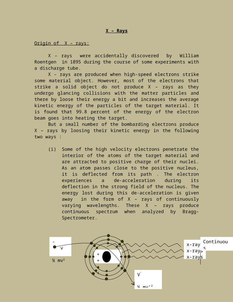
(i) Some of the high velocity electrons penetrate the interior of the atoms of the target material and are attracted to positive charge of their nuclei. As an atom passes close to the positive nucleus, it is deflected from its path . The electron experiences a de-acceleration during its deflection in the strong field of the nucleus. The energy lost during this de-acceleration is given away in the form of X – rays of continuously varying wavelengths. These X – rays produce continuous spectrum when analyzed by Bragg- Spectrometer.

(ii) Some of the high – velocity electrons while strike particularly the interior of the atoms of the target material, knock off the tightly bound electrons in the innermost shells (K, L-shells etc.) of the atoms. When the electrons from the outer orbits jump to fill up the vacancy so produced, out in the form difference is given out in the form of x-rays of definite wavelength. These wavelength constitute the line spectrum which is characteristic of the material of the target. Fig shows the case when these x-rays are emitted.

V’

½ mv’2

- v

½ mv2+ ++ +

x-raysx-raysx-rays

Continuous spectrum

KLM

X-rayK- line

X – ray diffraction

When a beam of monochromatic x-rays falls on a crystal it is scattered by the individual atoms which are arranged tin sets of parallel planes. Each atom becomes a source of scattered radiations. As we know from crystal structure, in every crystal there are certain sets of planes which are particularly rich in atoms. The combined scattering oof x-rays from these planes can be looked upon as reflections from these planes. Because of this, Bragg scattering is usually referred to as Bragg reflection and the planes as the Bragg planes. Because of these planes a crystal acts as reflection grating .

Bragg’s Law :

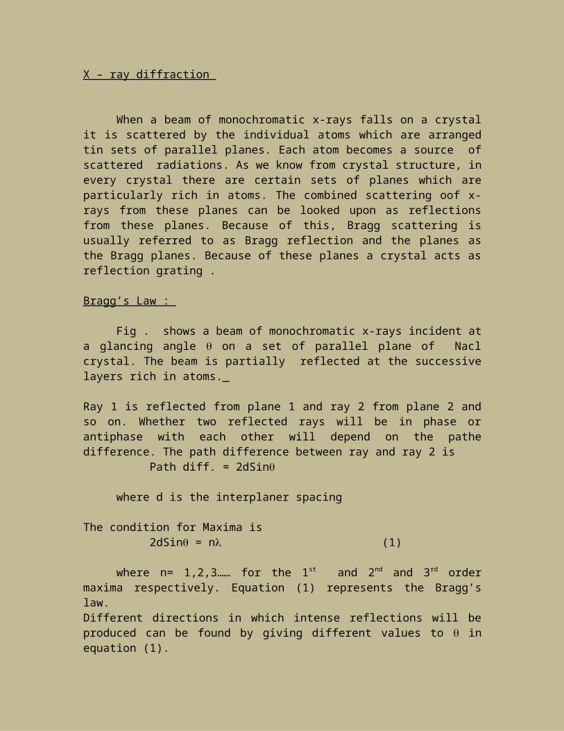
Fig . shows a beam of monochromatic x-rays incident at a glancing angle on a set of parallel plane of Nacl crystal. The beam is partially reflected at the successive layers rich in atoms.

Ray 1 is reflected from plane 1 and ray 2 from plane 2 and so on. Whether two reflected rays will be in phase or antiphase with each other will depend on the pathe difference. The path difference between ray and ray 2 is Path diff. = 2dSin

where d is the interplaner spacing

The condition for Maxima is 2dSin = n (1)

where n= 1,2,3…… for the 1st and 2nd and 3rd order maxima respectively. Equation (1) represents the Bragg’s law.Different directions in which intense reflections will be produced can be found by giving different values to in equation (1).

For the first Maxima, Sin1 = /2d

For the second Maxima, Sin2 = 2/2d

For the third Maxima, Sin3 = 3/2d etc.

Bragg’s law may be used to find the wavelength of x-ray if d is known. Conversely d may be computed if of x – ray is known from some other experiment.

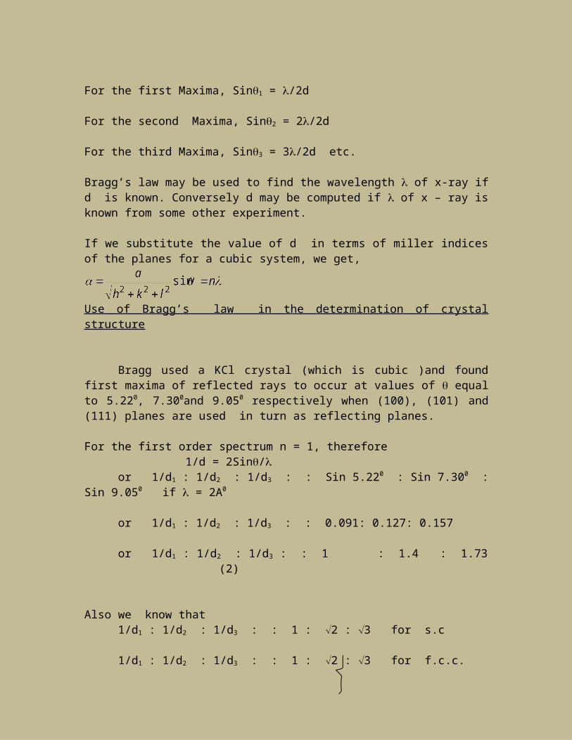
If we substitute the value of d in terms of miller indices of the planes for a cubic system, we get,

Use of Bragg’s law in the determination of crystal structure

Bragg used a KCl crystal (which is cubic )and found first maxima of reflected rays to occur at values of equal to 5.220, 7.300and 9.050 respectively when (100), (101) and (111) planes are used in turn as reflecting planes.

For the first order spectrum n = 1, therefore 1/d = 2Sin/

or 1/d1 : 1/d2 : 1/d3 : : Sin 5.220 : Sin 7.300 : Sin 9.050 if = 2A0

or 1/d1 : 1/d2 : 1/d3 : : 0.091: 0.127: 0.157

or 1/d1 : 1/d2 : 1/d3 : : 1 : 1.4 : 1.73 (2)

Also we know that 1/d1 : 1/d2 : 1/d3 : : 1 : 2 : 3 for s.c

1/d1 : 1/d2 : 1/d3 : : 1 : 2 : 3 for f.c.c.

1/d1 : 1/d2 : 1/d3 : : 1 : 2 : 3 for b.c.c. (3)

From equation (2) we get,

1/d1 : 1/d2 : 1/d3 : : 1 : 2 : 3

which shows K.C.l. to be a sample cubic structure.

X - Rays INTRODUCTION

The discovery of X-rays was accidental. A number of scientists were studying properties of cathode rays, amongst them W. C. Roentgen (1845-1923) noticed that a screen coated with barium platinocynide glowed brilliantly when it was brought near the tube in spite of a covered cathode ray tube. Thus this powerful radiation was discovered by Roentgen in 1895 and since its source was unknown it was called X – radiation . In Germany these rays are called Roentgen rays. The first Nobel Prize was awarded to Roentgen for his discovery, in 1901.

X-rays are electromagnetic waves having very short wavelength, of the order of a fraction of A0.

In 1912, Laue, Friedrich and Knipping, discovered X-ray diffraction by crystals. Max Von Laue (1879 - 1960) was a theoretical physicists, who requested Friedrich and Knipping, who were experimental physicists, to set up an experiment and observe X-ray diffraction. The discovery was a mile stone in the study of crystal physics. X-ray is a powerful tool in medical diagnosis.

Another important invention was the Coolidge X-ray tube developed in 1913. Earlier tubes were of the gas filed type , operated below 50 KV and were unsuitable for 100 to 200 KV. All modern tubes are Coolidge type tubes.

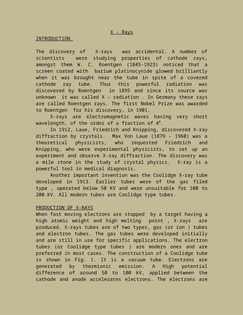
PRODUCTION OF X-RAYSWhen fast moving electrons are stopped by a target having a high atomic weight and high melting point , X-rays are produced. X-rays tubes are of two types, gas (or ion ) tubes and electron tubes. The gas tubes were developed initially and are still in use for specific applications. The electron tubes (or Coolidge type tubes ) are modern ones and are preferred in most cases. The construction of a Coolidge tube is shown in Fig. 1. It is a vacuum tube. Electrons are generated by thermionic emission. A High potential difference of around 50 to 100 kV, applied between the cathode and anode accelerates electrons. The electrons are focussed at the anode, where the target is mounted. Generally, molybdenum, tungsten etc. are used as the target. The target material should have a high melting point and high atomic number. In a target material having a high atomic number the yield is more.

coolant

ElectronX-ray

Thick copper anode

target

50 kV

Coolidge X-ray tube

The efficiency of an X-ray tube is given as

Efficiency = 1.4 X 10-9 ZVwhere V is the potential difference in volts applied between the cathode and anode and Z is the atomic number of the target material. Taking tungsten as a target Z = 74 and V = 100 kV say, the efficiency 1% . Thus 99% of the energy of the striking electrons is wasted i.e., converted to a very high level. Therefore, the melting point of a target material be high e.g. of tungsten it is 3370 0 C . A thick copper rod, used as an anode and a cooling system remove the heat generated at the anode. The rotating anode is used (for high intensity X-ray) production so that the electron beam will not strike the same portion of target surface. The target disc rotates slowly about its axis.

The X-ray spectrum is continuos, with a well defined cut-off . Along with this continuous spectrum, several sharp lines are observed. These sharp lines are called characteristics X-rays, as they are characteristics of the target material.

Continuous X-rays

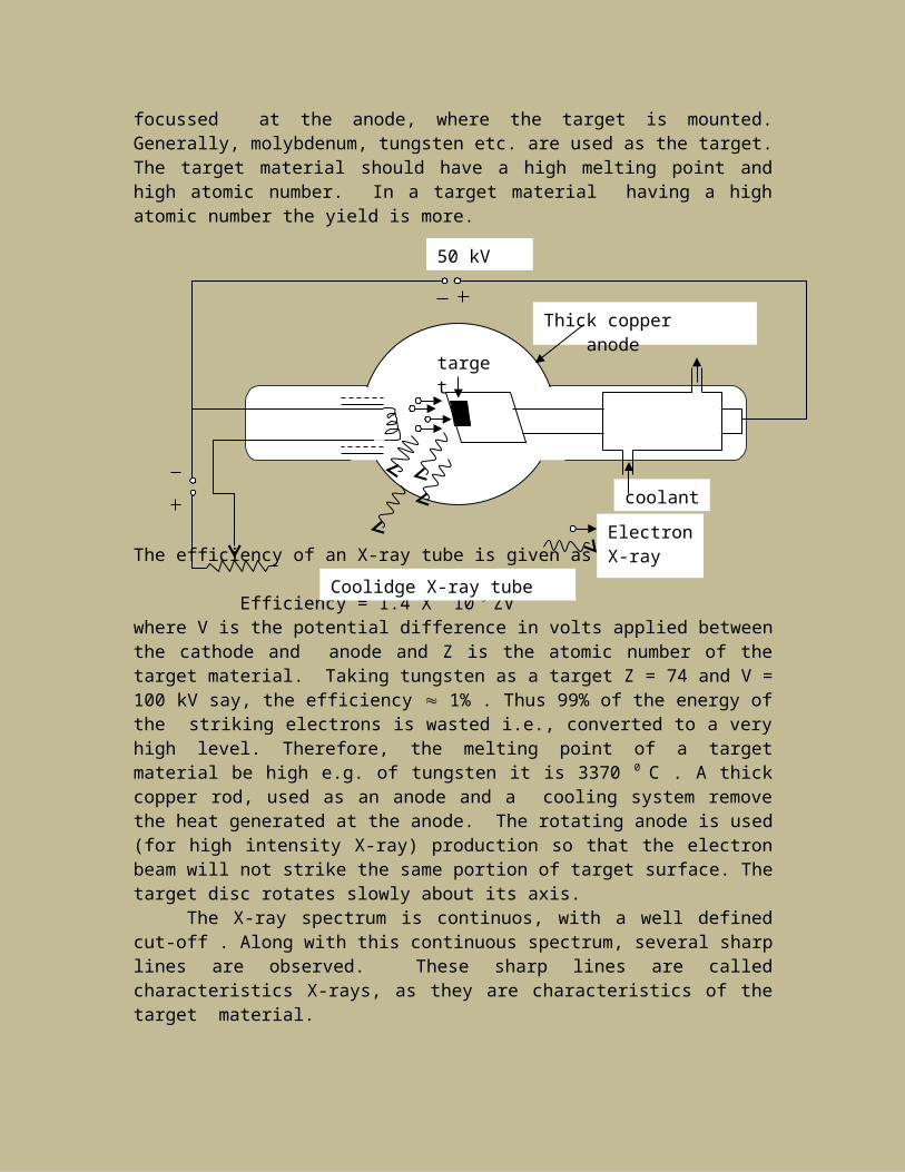
These X-rays depend upon the applied voltage between the cathode and the anode but do not depend, significantly, on the target material. As we have seen, most of the electron, striking the target material lose their energy in the form of heat and very few produce X-rays. An electron loses its energy as if brake applied, therefore these radiations are called braking radiations or Bremsstrashlung (A German word for breaking radiation).

Wavelength (Å)

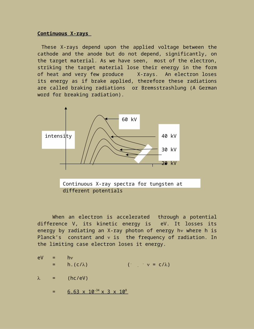
When an electron is accelerated through a potential difference V, its kinetic energy is eV. It losses its energy by radiating an X-ray photon of energy h where h is Planck’s constant and is the frequency of radiation. In the limiting case electron loses it energy.

eV = h= h.(c/) (.

. . = c/)

intensity 40 kV

30 kV

20 kV

60 kV

Continuous X-ray spectra for tungsten at different potentials

= (hc/eV)

= 6.63 x 10 -34 x 3 x 10 8 1.6 x 10-19 x V

.. . min. = 12431.25 x 10-10 m

V

Where V is the potential difference in volts, between the cathode and the anode of the X-ray tube.

Continuous X-rays are not only due to the radiation of photons. There are many mechanisms by which an electron loses energy e.g. excitation and ionization of atoms, displacement of atoms from their normal site in the crystal structure, large amplitude variations of the atoms etc.. The energetic electron may not lose its energy by creating a single photon but can create two or more photons. The photons can share the energy in an infinite number of ways.

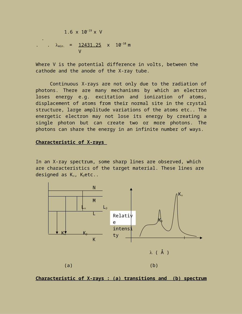
Characteristic of X-rays

In an X-ray spectrum, some sharp lines are observed, which are characteristics of the target material. These lines are designed as K, Ketc..

N K

M L L

L K

K K

K

( Å )

(a) (b)

Characteristic of X-rays : (a) transitions and (b) spectrum

In this case, striking electrons knock off any electron from an inner orbit and that vacancy is filled by another electron from a higher orbit. The system radiates the energy difference in the form of an X-ray photon.

The energy (and hence frequency or wavelength ) corresponding to a specific line such as K, L, etc. can be calculated, knowing the energies of the respective shells.

Relative intensity

Properties of X-rays

1. They are transverse electromagnetic waves.2. The radiations are invisible.3. They propagate in a straight line with the speed of light. 4. They are unaffected by the electric or magnetic fields.5. They have wide wavelength range, from 0.01 Å to 1000 Å.6. They can be reflected, refracted diffracted and polarized with a suitable

arrangement.7. They blacken a photographic plate.8. They ionize a gas.9. They affect electric properties of solids and liquids.10. They can liberate photoelectrons or cause the electrons to recoil.11. They produce fluorescence and phosphorescence. 12. They can act photochemically.13. They can kill or damage living cells.14. They produce genetic mutations.15. They have a high penetrating power and can pass through paper, flesh etc..

X-ray diffraction

As we have noted in the beginning , the discovery of X-ray diffraction by Laue and others was a major advancement in the study of solid state physics.

Regularly spaced planes of atoms in a crystal can act as a diffraction grating. The wavelength of X-rays being very small, diffraction can be observed using a crystal grating. Thus, X-ray diffraction permits the observations of the interior of solids, which help in understanding and predicting different properties. Uses of X-ray diffraction

1. Atomic distances and atomic radii can be determined.2. Defects in the structure can be detected.3. The shape and the structure of the organic molecules can be studied.4. Quartz crystals can be oriented to cut piezoelectric plates.5. Textile, plastic, rubber etc. can be studied.

Applications of X-rays Materials having high melting points, greater strength and specific electric properties are always needed for various purposes. Their optical, mechanical, thermal and electrical properties are related to their crystal structure. Crystallography using X-rays is an important tool for this. As we have seen X-ray diffraction has many applications. X-ray diffraction permits the observation of the interior of the solids in crystallography and metallography. In latter it is used to determine the appropriate method of manufacturing

and maintain constant properties of metal or alloy. The analysis of mechanisms obtained from x-ray diffraction pattern helps in heat treatment and recrystallization of metals.

Obtaining shadow patterns of the internal structure of bodies using X-rays is called Radiography . Radiography is somewhat similar to photography. In a photograph, optical shadows, distinguish completely opaque and transparent portions, whereas in a radiograph varying degrees of transparency are observed. The radiologist, in metallurgy or medicine, interprets the radiograph on the basis of his knowledge of the object and X-rays.

Radiography is a useful tool in the study of phase change, inspection of rivets and concealed components, detection and identification of defects in casting and welding etc..Radiography is a used in examining paintings, to reveal the technique of brush work, development stages, overpainting, alteration, condition of an old painting, etc..

The bone absorbs more radiation than soft tissue, therefore, in radiography, fractures, foreign bodies etc. can be detected. The soft tissue radiographs are used for breast examination, Lipomas and calcification examination etc.. In dentistry, radiography is also useful diagnostic tool.

X-rays are used in killing malignant cells. Some of the diseases and conditions can be treated with radiotherapy (therapeutic use of X-rays) e.g. cancer, skin diseases, spondylitis etc..

Technological Properties

1) Weldability2) Machinability3) Formability4) Castability

1) Weldability:

Welding is a material joining process used in making joints. By definition a weld is the coalescence of one metal with another by application of heat or some other form of energy. Thermoplastics can be welded with a hot air torch, and some plastics can be solvent welded, but in general welding is applied to metals more often than in plastics.

The term ‘weldability’ has been defined as the capacity of a metal to be welded under the fabrication conditions imposed in specific suitably designed structure and to perform satisfactorily in the desired service.

The primary factors that control the weldability of metals are chemical composition, the basic metal composition and the composition of the filler metal. A metal with good weldability can be welded readily so as to perform satisfactorily in the fabricated structure.

A fusion can not be made between two dissimilar metals unless they have metallurgical solubility. Titanium can not be welded to most metals because it is not soluble in most other metals. Phase diagrams can be consulted to determine if dissimilar metals can be welded. If the phase diagram show low solid solubility, the weld can not be made. The combination will have poor weldability.

Poor weldability will be manifested by such thing as cracking of the weld, porosity, cracking of the heat affected zone, and weld embrittlement. Weldability problems due to many varied causes.

i) Metals with high sulpher contents crack in the weld because sulpher causes low strength in the solidifying metal (hot shortness).

ii) Welding of rusty or dirty metals can cause weld porosity.iii) Welding copper with high oxygen content causes embrittlement.iv) Welding of hardenable steels can lead to cracking in the heat –

affected zone (HAZ).

Of all the potential weldability problems that can occur, two stand out as the most common and most troublesome.

(1) Arc welding resulfurized steels (2) Arc welding hardenable steels

1) High – sulfur steels (. 3%) arc widely used for parts that require significant machining. They save money they are rent aid in lowering material cost. However, there is no way to avoid weld-

cracking problems with these steels other than to establish a hard and fast rule never to arc weld them. Brazing and soldering is acceptable, but not arc welding to themselves or to other metals.

2) Welding hardenable steels causes a weldanability problem because there is a high risk of cracking in the weld or adjacent to the weld. When a weld is made, it and the heat affected zone go through a thermal cycle not unlike a sequence hardening cycle. It makes no difference whether the parts are hardened or soft before welding. Melting of steels requires a temperatures of about 30000F (15400C). The hardening temperature (ansterilizing) temperature ranges from 1500 to 20000 F(8150C to 10930 C) . Obviously the weld is going to be cycled in this temperature range, as is some of the metal adjacent of the weld. The mass of the metal to be welded serves as a quenching media and hard martensite will form either in the weld, heat-affected zone, or both. This structure will be brittle, and if the weld is under restraint the brittle structure will crack. It cannot deform.

In deciding weldability of a metal, the most common characteristics to be noted are i) Heating and cooling effects on the metalii) Oxidationiii) Gas vaporizationiv) Solubility

i) Heating and cooling effects:The effect of heat in determining the weldability of a

material is related to the change in the micro-structure that results. For example, steels are sometimes considered weldable or not weldable on the basis of the hardness of the weld. The deposition of the weld metal may pick up carbon or other alloys and impurities from the parent metal that make it hard and brittle so that cracks result upon cooling. Reverse is also possible. A metal may have certain hardness temper that will be changed by the heat of the weld. Hot-shortness a characteristic which is indicated by lack of strength at high temperatures , may result in weld failure during cooling of certain materials.

ii) Oxidation:Metals that oxidize rapidly at elevated temperatures, such

as aluminium, interfere with the welding process as the oxides have the higher melting point than the base metal. This prevents the metal from flowing. It may also become entrapped in the weld metal resulting in porosity, reduced strength, and brittleness.

iii) Gas :Trouble some gases produced during the welding process

may become entrapped in the weld because certain element vaporize at temperature below the welding temperature. This will cause the porosity.

(2) Machinability:

It has been used in many ways to describe properties of materials when they are cut (1) It is defined as the case with which a given material can be cut permitting the removable of the material with a satisfactory finish at the lowest cost. (2) In another sense, Machinability may be used o signify how long a welding lasts with material as compared with others under standardized conditions. (3) A third meaning implies how well a material takes a good finish. (4) A fourth one indicates the amount of power necessary for a given cut.

Ease of metal removable implies, among other things that the forces acting against the cutting tools will be relatively low, the chips will be easily broken up, that a good finish will result and that the tool will last a reasonable period time before it has to be replaced or resharpened.

Machanibility depends upon :

(1) Chemical composition(2) Microstructure(3) Mechanical properties(4) Physical properties(5) Cutting conditions

Most common factors affecting the Machinability are –(1) Chemical composition: - For example steel with specific chemical

composition will vary in the machinability depending on its method of heat treatment. Steels with different alloys will have different machinability. Presence of smaller amount of lead, manganese, sulpher, phosphorus is advantageous.

(2) Microstructure:- Uniform Microstructure helps in machining. Non-uniform microstructure decreases machinability.

(3) Mechanical properties:- Low hardness, low ductility and low strength provides better machinability. Hot working of hard alloys e.g. medium and high carbon steels, cold working of low carbon steels, annealing, normalizing and tempering helps in machining.

The main factors used for judging machanibility are :(1) Tool – life between grindes.(2) Value of cutting forces(3) Quality of surface finish(4) Form and size of finish

(5) Temperature of cutting(6) Rate of cutting under multiple forces (turning, forming, milling,

drilling etc.)(7) Rate of metal removable(8) Consumption of power.

Machinability Index :

Machinabilty index , %

= Cutting speed of metal investigated for 20 min. tool lifeCutting speed of a standard steel for 20 min. tool life

Machinability of standard steel is given an arbitrary value of 100 % machinability. Its composition is –

Carbon -- 0.13 % maxm.Manganese -- 0.06 to 1.10 % Sulpher -- 0.08 to 0.03 %

(3) Formability

The ability of metal to be formed is based on ductility of the metal which in turn is based on its crystal structure.

Formability thus can be explained on the basis of ductility.Formability is affected by the following factors :

(1) Grain Size – Single crystals will have non-interfacing slips, where as poly crystals will have interfacing slips. Thus Single crystals will have higher ductility.Small grain sizes are recommended for shallow drawing of copper, and relatively large grains are recommended for heavy drawings on the thicker ganges.

(2) Hot and cold working : - Hot working affects the grain sizes. The ductility will depend on the extent of distribution. Cold-working also distarts the crystal and the distortion is more than in the hot working. Hence cold worked metal will have less ductility.

(3) Alloyingelements : - Prevents sips, thus less ductile.(4) Softening heat treatment : - Annealing consists of heating the metal

to the recrystallization temperature. The grains grows in size form a smaller to a desired size and then the metal is cooled. During recrystallization the ductility of the metal is restructured.

(4) Castability

The case at which a metal can be cast into forms is known as the castibility of metal. Factors governing are :

1) Solidification rate :- The case at which a metal will continue to flow after it is powered in the mould. Some metals like gray iron can be poured in to thin sections of complex coatings where as others like tungsten and molybdenum cause casting problems because of their high melting temperatures.

2) Shrinkage – It is the reduction in volume of a metal when it goes from a molten to a solid state. This should be controlled by suitable additions of other elements .

3) Segregation - As metals starts to solidify, tiny crystal structures, starts forming at the edges and they tend to avoid alloying elements. However subsequent crystals that form are richer in alloy content as the metal solidifies. Thus the casting is not uniform. This is overcome by subsequent heat treatment.

4) Gas – porosity – Some gases like oxygen and nitrogen may get trapped and produce voids.

Low hot strength

Metal are very low in strength right after solidification. Precautions must be taken to reduce stress concentration during casting so that flaws do not develop.

Gray iron : - Gray cast iron is an alloy of iron, carbon and silicon that is not malleable in a cast condition. The carbon content varies from 2.5 to 4% and the silicon content from 1 to 3 %.

And cast iron is suited for the production of intricate castings because of its high fluidity at casting temperatures and its low shrinkage. Other properties are

Damping capacity -- excellentResistance to wear and seizure -- highNotch reusability -- lowMachinability -- lowCost and availability -- low and readily available

Brittle Fracture – Griffith Theory

Brittle fracture takes place with little or no preceding plastic deformation. It occurs, often at unpredictable levels of stress, by the sudden propagation of a crack. Amorphous materials, such as glass and glassy polymers, we completely brittle; in crystalline materials. However, some plastic deformation proceeds brittle fracture.

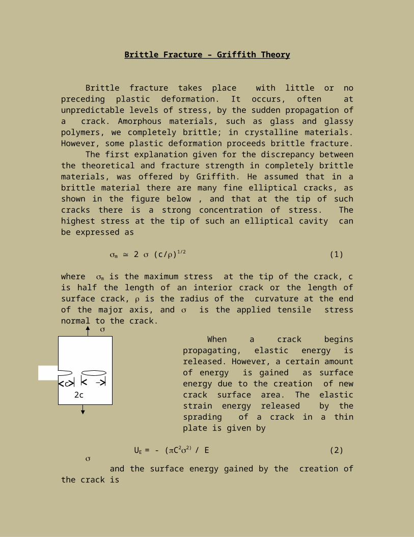
The first explanation given for the discrepancy between the theoretical and fracture strength in completely brittle materials, was offered by Griffith. He assumed that in a brittle material there are many fine elliptical cracks, as shown in the figure below , and that at the tip of such cracks there is a strong concentration of stress. The highest stress at the tip of such an elliptical cavity can be expressed as

m 2 (c/)1/2 (1)

where m is the maximum stress at the tip of the crack, c is half the length of an interior crack or the length of surface crack, is the radius of the curvature at the end of the major axis, and is the applied tensile stress normal to the crack.

When a crack begins propagating, elastic energy is released. However, a certain amount of energy is gained as surface energy due to the creation of new crack surface area. The elastic strain energy released by the sprading of a crack in a thin plate is given by

UE = - (C22) / E (2)

and the surface energy gained by the creation of the crack is US = 4c (3)

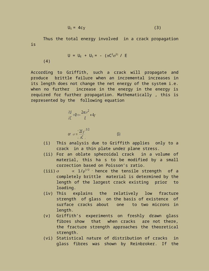
Thus the total energy involved in a crack propagation is

U = UE + US = - (C22) / E (4)

According to Griffith, such a crack will propagate and produce brittle failure when an incremental increases in its length does not change the net energy of the system i.e. when no further increase in the energy in the energy is required for further propagation. Mathematically , this is represented by the following equation

c 2c

(i) This analysis due to Griffith applies only to a crack in a thin plate under plane stress.

(ii) For an oblate spheroidal crack in a volume of material, this ha s to be modified by a small correction based on Poisson’s ratio.

(iii) 1/1/2 , hence the tensile strength of a completely brittle material is determined by the length of the largest crack existing prior to loading.

(iv) This explains the relatively low fracture strength of glass on the basis of existence of surface cracks about one to two microns in length.

(v) Griffith’s experiments on freshly drawn glass fibres show that when cracks are not there, the fracture strength approaches the theoretical strength.

(vi) Statistical nature of distribution of cracks in glass fibres was shown by Reinbroker. If the glass fibre is successively fractured, thus progressively eliminating the most serious cracks; strength was increased by a factor of two or three.

(vii) Similarly, if rich sheets were subjected to stress with grips narrower than the width of the sheet, the tensile strength of the mica was found to be ten times greater . This was due to the stress being concentrated in the centre of the sample., and not in the edges where the surface cracks are present and thus, preventing the surface from propagating.

Brittle Fracture in Crystalline materials :

The above theory is amorphous materials. For crystalline materials, plastic deformation usually occurs next to the fracture surface.

Therefore, the energy here will have three contributors (i) Elastic energy(ii) Surface energy due to new surface area created.(iii) Energy required for plastic deformation the vicinity of the crack.

Orowan has shown that when the plastic deformation is concentrated in the region whose thickness is small compared to the length of a crack, the work of plastic deformation may be treated as a contribution to the effective surface energy of this crack. Recognizing this , Griffits equation may be modified as

where p is the work of plastic deformation at the tip of the growing crack. can be neglected compared to p as the value of p for low-carbon steel which have failed in brittle manner range from 105 to 106 ergs /cm2, approximately one thousand times greater than the true surface energy.

Ductile Fracture:

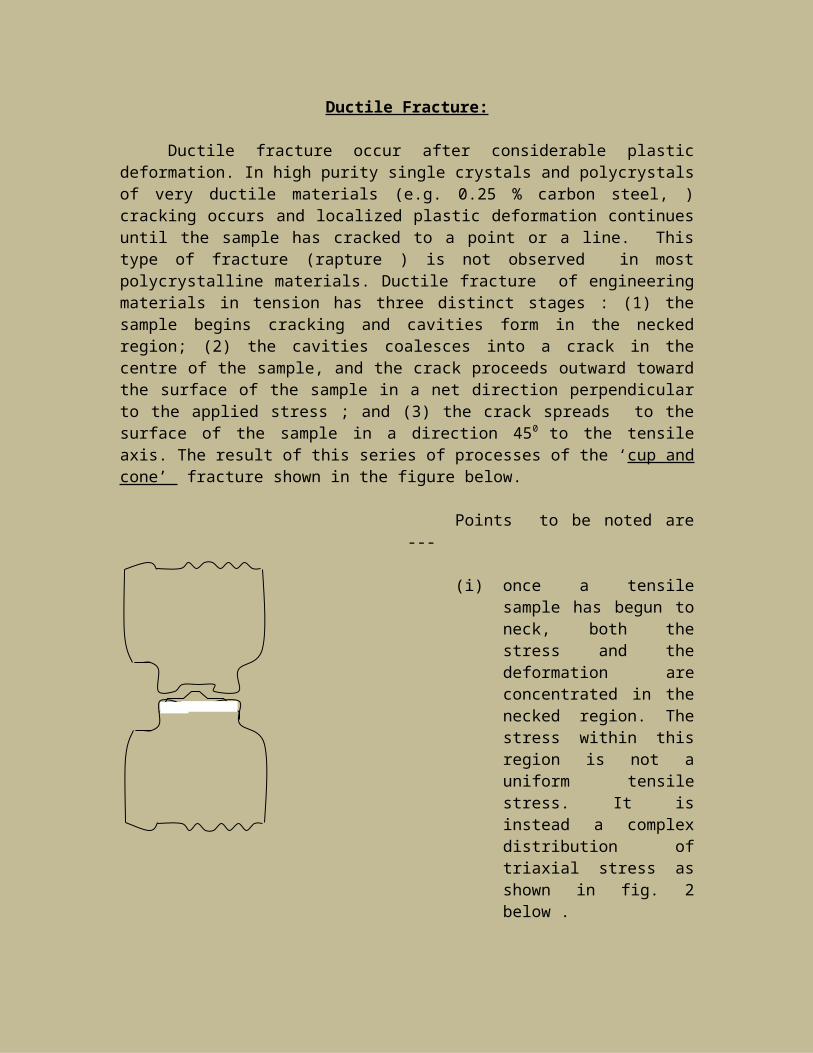
Ductile fracture occur after considerable plastic deformation. In high purity single crystals and polycrystals of very ductile materials (e.g. 0.25 % carbon steel, ) cracking occurs and localized plastic deformation continues until the sample has cracked to a point or a line. This type of fracture (rapture ) is not observed in most polycrystalline materials. Ductile fracture of engineering materials in tension has three distinct stages : (1) the sample begins cracking and cavities form in the necked region; (2) the cavities coalesces into a crack in the centre of the sample, and the crack proceeds outward toward the surface of the sample in a net direction perpendicular to the applied stress ; and (3) the crack spreads to the surface of the sample in a direction 450 to the tensile axis. The result of this series of processes of the ‘cup and cone’ fracture shown in the figure below.

Points to be noted are ---

(i) once a tensile sample has begun to neck, both the stress and the deformation are concentrated in the necked region. The stress within this region is not a uniform tensile stress. It is instead a complex distribution of triaxial stress as shown in fig. 2 below .

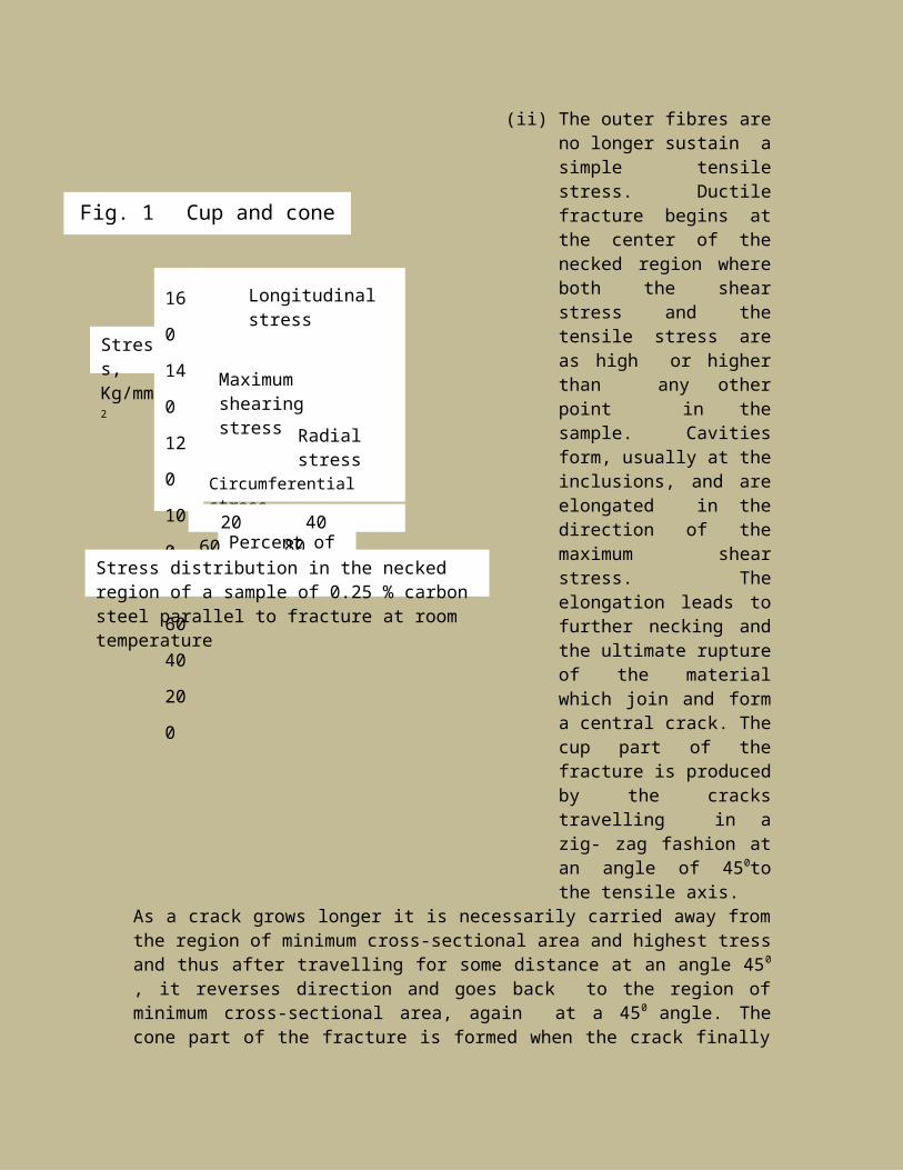
(ii) The outer fibres are no longer sustain a simple tensile stress. Ductile fracture begins at the center of the necked region where both the shear stress and the tensile stress are as high or higher than any other point in the sample. Cavities form, usually at the inclusions, and are elongated in the direction of the maximum shear stress. The elongation leads to further necking and the ultimate rupture of the material which join and form a central crack. The cup part of the fracture is produced by the cracks travelling in a zig- zag fashion at an angle of 450to the tensile axis.

Fig. 1 Cup and cone fracture

Percent of Radius

Stress, Kg/mm2

160

140

120

100

80

60

40

20

0

Longitudinal stress

Maximum shearing stress

Radial stress

Circumferential stress

20 40 60 80 100

Stress distribution in the necked region of a sample of 0.25 % carbon steel parallel to fracture at room temperature

As a crack grows longer it is necessarily carried away from the region of minimum cross-sectional area and highest tress and thus after travelling for some distance at an angle 450 , it reverses direction and goes back to the region of minimum cross-sectional area, again at a 450 angle. The cone part of the fracture is formed when the crack finally progresses close enough to the surface of the sample that the sample separates by shear fracture at an angle of 450 to the tensile axis. Although the ‘cone’ portion of the fracture appears , microscopically, to be smaller than the ‘cup’ portion, electron microscopy shows that both are made by the same process of coalescence of cavities.

Types of Magnetism

Magnetism B = H (1)B =0r H r = / 0 (2)M =m H (3)m= M/ H Susceptibility (4)B =0 (H + M) (5)

Types of Magnetism

(i) Diamagnetism(ii) Paramagnetism(iii) Ferromagnetism(iv) Antiferromagnetism(v) Ferrimagnetism

(i) Diamagnetism : For simplicity a circular orbit is assumed with a single electron having an angular velocity . This angular velocity is altered if a magnetic field is applied slowly the radius of the orbit being unaltered. The change in angular velocity gives rise to a magnetic moment m of magnitude

e2

m = 0r2 A (6)4m

where e = electron chargem = mass of the electronr = radius of the orbitH = applied field.

The susceptibility is given by

m= - M/ H (7)

It is small and negative i.e. the atomic susceptibility is small. For orbits of radius of about 1A, the factor e20 r

2 / 4m ~ 10-34 m3 . Since an average solid has about 1028 to 1029 atoms per cubic meter, the volume susceptibility m ~ 10

-5 to 10-6 . It is independent of temperature.

m

m = vol./atom Example : Zn, Cd, Hg, Sb, Bi, Au, Cu, Hg, Xe, etc..

Material m Material n

Au -8.7 X 10-5 Diamond -2.1 X 10-5

Cu -0.95 X 10-5 NaCl -1.2 X 10-5

Hg -2.9 X 10-5 Water -0.9 X 10-5

Xe -25.0 X 10-9

(ii) Paramagnetism :

= C/T ---- Curie law (8)

here is small but positive

Material Material Air 0.038 X 10-5 CO 5.80 X 10-5

Al 2.3 X 10-5 Nitrogen 0.0013 X 10-5

Ebonite 1.4 X 10-5 Oxygen 0.19 X 10-5

Curie – Wies Law = C/(T-) (9)

Temperature dependent

m = (N0 2m )/ 3KT

= C/T (10)

where C = (N0 2m) / 3K (11)

More examples of paramagnetic Solids -- Fe, Ni, CO, Mn, Mg, Cr.Gases -- No, NO2, ClO2

Sulphates and chlorides f Ni, Co, Mn, Fe, Cr, etc..

Ferromagnetism

= C/ (T-C)

Extra term HW = M

M / (H + HW ) = C/ T

Or, M / (H + M) = C/ T

Or, (H + M) / M = T / COr, H / M = T / (C -) = (T - C) / C

Or, Ferro = C / (T - C).

Prefened Orientation

P- 221 Choudhary

Prefened orientation is said to occur with in a metal when certain lattice directions in the grains are aligned with the principal direction of flow under severe deformation. Its nature and manner in which it is accomplished are characteristics of the metal and the type of deformation. In other words, a metal which has undergone a severe amount of deformation, as in rolling or wire drawing, will develop Prefened Orientation, or ‘Texture’ in which certain crystallographic planes tend to orient themselves in a prefened direction with respect to direction of maximum strain. This prefened orientation may be responsible for very directional properties in some materials. It is particularly common in metals subjected to rolling or drawing to produce sheets or wires because the crystallites tend to align themselves with a major axis parallel to the rolling or drawing direction. It also produces considerable anisotropy in the physical properties, which may affect subsequent fabrication of components. However, it not always disadvantageous. For examples in transformer laminations, anisotropy due to PO is preferable provided the sheets can be aligned with their easy direction of magnetization.

The Fe/3 percent Si alloy used for the laminations of transformer core is deliberately given thermal/mechanical treatments that bring about a strong degree of magnetic anisotropy which improves electrical performance of transformers. In the bcc iron, it is easier to magnetize the material to saturation in the directions parallel to the cube edges, (<100> directions) than the <111> directions.

<100> Easy direction

BTesla

<111>Head direction

0 15,000 30,000H(amp/m)

Prefened orientation resulting from deformation is strongly dependent on slip and twinning systems available for deformation. Planes of slip in all the crystals are caused to rotate into more favorable directions with respect to the direction of maximum shear stress.

Prefened orientation is not affected by process variables such as die angle, roll speed, reduction per pass etc. The most important parameter is the direction of flow .

During cold drawing of Aluminium wire, for example, grains that that were initially oriented at random are deformed in such a way that they have a [111] crystal direction along the wire axis.

Prefened orientations are determined by x-rays methods. The x-ray pattern of afine grained randomly oriented metal will show rings corresponding to the different planes where the angles satisfy the Bragg’s reflections.

If the grains are randomly oriented, the intensity of the rings will be uniform at all the angles., but if a prefened orientation exists, the rings will be broken up into short arcs or spots.

Although some directional properties are advantageous. For example, because of anisotropic of plastics properties, sheets with prefened orientation are not suitable for deep drawing, because unequal flow leads to local thinning and ears are formed. An ear represents a direction in which the resistance to deformation is relatively low.

RandomPrefened Orientation

Season Cracking

In addition to the changes in the physical and chemical properties , internal stresses often of very high intensity, may be left in an object after cold deformation. Metals such as brass with internal stresses appearing after cold cracking is susceptible to intercrystalline corrosion, if it is stored for a long period. This leads to a type of failure of the material known as season cracking.

It is a kind of cracking encountered in certain cold worked ( ZO u/3.0 Zn) brasses, resulting from the combined effect of a corrosive environment and residual stresses within the metal.

Season cracking may be eliminated by annealing strain – hardened brass at 2000 – 3000 C for several hours. Season cracking develops readily in corrosive environment.

Bauschinger Effect

The Bauschinger Effect was discovered by Johann Bauschinger in 1886. If in a metal, the plastic flow is started at a certain stresses under tension (+ve stress) in one slip –system, and subsequently the stress is reversed (-ve, compression), then plastic flow is observed to start initiate at a lower stress level. This phenomenon of reduction in the yield strength of a material under reversal of direction of stress is called Bauschinger Effect. Figure – 1 below illustrates Bauschinger Effect.

Let a material have the yield stress in tension as ‘a’ and thanthe same in compression ‘x’. If a new specimen of the material Is loaded in the tension.

c

b

+

-

d

a

O

e

x

- +

Mechanical Properties and Testing

1. Fundamental properties :

The mechanical properties of materials, as defined earlier, shows the behavior of the materials under the action of external forces called loads, and most of them are “structure – sensitive”. However, some of them are the subject of standardized tests are best defined in terms of these tests, while some properties are regarded as fundamental and can be explained in a qualitative way. It is therefore, logical to start with the fundamental mechanical properties of materials.

Strength

The strength of a the material is its capacity to withstand destruction under the action of external loads. The stronger the material the greater the load it can withstand. It, therefore, determines the ability of a material to withstand stress without failure. Since strength varies according to the type of loading, it is possible to access tensile, compressive, shearing or torsional strengths.

On the basis of bonding forces, we can say that the materials with pure covalent bonding would be strongest and that those with pure ionic bonding would be nearly as strong . Metallic bonding would be clearly third and molecular bonding would be weakest.

Elasticity:

Elasticity is that property of a material by virtue of which deformations caused by applied load disappear upon the removal of the load. In other words, the elasticity of a material is its power of coming back to its original position after deformation when the stress or load is released. The recoverable nature of elastic deformation makes it possible to store elastic energy in solids and to release its under controlled conditions. Elasticity of the solids has its origin in the existence and the stability of interatomic and intermolecular bondings.

In accordance with the concept of the elastic behavior, the quantitative measure of the elasticity of a material might be expressed as the extent to which the material can be deformed within the limit of the elastic action. Since the engineers think in terms of stress rather than of strain, a practical index of elasticity is the stress that marks the effective limit of elastic behavior.

Stiffness:

The resistance of a material to elastic deformation or deflection is called stiffness. A material which suffers slight deformation under load has a high degree of stiffness. For instance, suspended beams of steel and aluminium may both be strong enough to carry the required load but the aluminium beam will “sag” or deflect furhter. In other words, the steel beam is stiffer than aluminium beam.

If the material follows Hook’s law, i.e. has a linear stress- strain relation, its stiffness is measured by the Young’s modulus E, also variously termed the “” or “modulus of elasticity”, found geometrically from the stress-strain diagram by measuring the slope of the straight line, since E = /. The stiffness of a material that does not follow Hook’s law is clearly not constant, but varies with stress. Sometimes the average stiffness is the best measure this quantity at a given stress. It is given by the scant modulus and represents the average slope of the curve.

The term “flexibility is sometimes used as the opposite of stiffness. However, flexibility usually has to do with flexure or bending. Also it may connote ease of bending in the plastic range. The effective or overall stiffness or rigidity or flexibility of a body or structural member is obviously a function of the dimensions and shape of the body as well as of the characteristic of the material.

ResilienceResilience is the capacity of a material to absorb energy elastically, when a body is loaded without exceeding the elastic limit, it changes its dimensions, and on the removal of the load it regains its original dimensions. In fact, the body behaves perfectly like a spring. So long as it remains loaded, it has strong energy in itself, which is called the strain or the internal energy. On removal of the load, the energy stored is given off exactly as in a spring when the load is removed.

The maximum energy which can be stored in a body up to the elastic limit is called the proof resilience. In other words, the energy stored per unit volume at the elastic limit is the modulus of the resilience. This quantity is the mechanical property of the material, and gives the capacity of the material to bear shocks and vibrations.

Materials that have high resilience is used for springs. Annealed copper should make poor spring because its elastic limit is very low, but cold-work copper has a much higher elastic limit and resilience and, therefore, makes a better spring. Thus high resilience is associated with high elastic limit.

Plasticity :

The plasticity of the material is its ability to undergo some degree of permanent deformation without rupture. Plastic deformation will take place only after the elastic range has been exceeded. A general action for plastic action would involve the time rate of strain since in the plastic state materials can deform under constant sustained stress. It would also involve the concept of limit of deformation before rupture. Evidence of plastic action in structural materials are called yield, plastic flow, and creep.

Plasticity is important in forming, shaping and extruding operations. Some materials are shaped cold, e.g. the deep drawing of sheets. Many materials particularly metals are shaped hot, e.g. the rolling of the structural steel shapes and the forging of certain machine parts. Materials such as clay, lead, etc. are plastic at room temperature, and steel is plastic when at bright red heat. In general, plasticity increases with increasing temperature.

Ductility and Malleability :

Ductility is the property of the materials which enables it to draw out. Into thin wire. Mild steel is a ductile material. The percent elongation and the area in tension are often used as empirical measures of ductility.

Malleability of a material is its ability to be flattened into their sheets without cracking by pressing, rolling, hammering etc. Aluminium Copper, Lead, tin etc. , are malleable metals.

Current usage of the words ductility and malleability makes it almost synonymous with workability or formability which is clearly related to plastic deformation. However it is important to realize that some material may be malleable and not ductile. Lead, for instance can be readily rolled and hammered out but cannot be drawn into wire. Although ductility and malleability are frequently used interchangeably, ductility is thought of as a tensile quality, whereas the malleability is considered as a compressive quality.

Toughness:

The toughness of a material is its ability to withstand both plastic and elastic deformation. It is in fact, the amount of energy a material can be absorb much more energy before failure occurs. Thus a mild steel is said to be much tougher than a glass. Toughness, is therefore, a highly desirable quality for structural and machine parts which have to withstand shock and vibration. Manganese steel, wrought iron, mild steel, etc. are tough materials.

Although it is nearly impossible to measure toughness in absolute units, it is usually represented by the area under a stress-strain curve and thus involves both strength and ductility. The total area under the stress-strain curve is work expended in deforming one cubic meter of the material until it fractures. This work of energy is sometimes called the modulus of toughness. Toughness is related to impact strength i.e. resistance to shock loading, but there is no definite relationship between the energy values obtained from static and impact testing.

Hardness, Hardenability and Brittleness :

The hardness of a material is difficult to define as a distinct property because it is closely associated with material structure, composition, and other mechanical properties. Consequently, the word hardness has been used to define many things. Hardness has been described by the words vigorous, stout, rugged, hardy, firm, and compact. Even in technology hardness has been measured in various ways and, depending upon the field of science or engineering considered, hardness measures different properties. That is, harness may represent the ability of a material to resist scratching, abrasion, cutting, or penetration. In minerology and ceramics, the ability to resist scratching is used as a measure of hardness. In other words, the type hardness considered depends upon the service requirements to be met. For example, many structural and machine parts such as rails, gears and axles are subjected to service requirements where a high resistance to indentation

is desirable. Sometimes the hardness of a material is measured by its ability to absorb energy under impact loads. Hardness, as measured by resistance to abrasion, is also a measure of the wearing quality of a material. When hardness is measured by resistance to cutting , an induction of machinability qualities of the material is obtained.

Many methods are now in use for determining the hardness of material . They are Brinell, Rockwell and Vickers. For more hardness test, however, in as much as the stress conditions are complicated and cannot be evaluated, the hardness is simply expressed in terms of some arbitrary values, such as the scale reading of the particular instrument used.

Hardenability indicates the degree of hardness that can be imparted to a metal particularly steel, by the process of hardening. It determines the depth and distribution of hardness induced by quenching. Hardenability should be differentiated from hardness which is the property of a material which represents its resistance to indentation or deformation. Hardness is associated with strength, while herdenability is concerned with the transformation characteristics of a steel. Hardenability may be increased by the transformation kinetics by the addition of the allowing elements, while the hardness of a steel with given transformation kinetics is controlled primarily by the carbon content.

The brittleness is the property of breaking or shattering without much permanent distortion. There are many materials which shatter before much deformation takes place; such materials are brittle. Glass and cast iron are good examples of brittle materials. Hot or red hotness in steel, is when it is brittle in the red-hot state. Cold shortness means that the metal is brittle when cold. The lack of ductility is commonly called brittleness. Therefore, a non-ductile material is said to be brittle material. Usually the tensile strength of brittle materials is only a fraction of their compressive strength.

Dislocations

Dislocations in a crystal is a linear defect. They are distinct from point defects in being extended in one dimension and are therefore referred to as line defects. Although they are frequently observed in electron microscope to be reasonably long and straight and to lie on crystal planes of high packing density, these requirements are not inevitable. The characteristics of the line defects are is that in its immediate neighborhood the interatomic bonding is distorted and the local stored elastic energy of the defect is quite high, since the bonds are already locally distorted it requires less additional effort to break them than it would if the lattice were perfect . As a result of this, most dislocations can therefore move easily through a lattice under relatively small applied stresses.

Dislocations may occur during growth of crystals, from a melt or from a vapor, or they may be produced during the slip. The idea of such defects in crystalline material was first postulated, quite hypothetically, in order to explain the discrepancy between the calculated and observed strengths of metallic materials. However, since the first introduction of the hypothesis about 1930, the existence of dislocations in real crystal has been adequately proved by electron microscopy. Due to existence of these defects, we shall see, most metals are substantially weaker than the intrinsic intra atomic bond strength would lead us to expect. Only a lattice without dislocations would be ideally strong, but since all crystalline materials, especially those that have been produced by usual manufacturing processes, contain many dislocations (10 8 dislocations per square centimeter in the annealed state), the crystals are weaker than it is expected on the basis of intrinsic interatomic bond.

The need to introduced dislocations to account for the shear strength of real crystalline is justified by the following considerations.

A crystalline material such as metal can be visualized as being composed of planes or layers of atoms, the orientation of which are described by Miller Indices. As a result, when a stress is applied, it is natural that atomic movements would take place. These movements lead to the plastic deformation in the macroscopic level. But in a metal, such deformation takes place without fracture. This means that atoms must at all times have remained within one intratomic distance of each other. These movements must therefore involve a slipping or shearing of one or one plane of atoms over another. If we assume the lattice to be perfect, it should be possible to calculate the stress needed to cause this shearing of the planes.

Fig. Below illustrates a perfect crystal in which arrangement of atoms is represented by two rows :

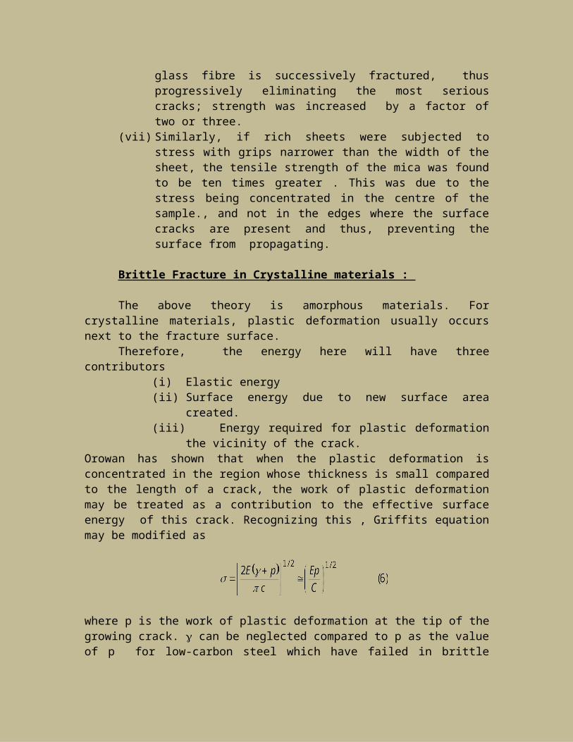
Fig. 1 vibration of shearing stress : (a) displacement of atoms in respect to interatomic distances, (b) periodic shearing stress as a function of the displacement of atoms. The shear stress necessary to produce slip by a distance x will be a function of the displacement of atoms.

The shear stress necessary to produce slip by a distance x will be a function of x. By analyzing the system it can be seen that the shear stress will vary sinusoidally. If the distance between the rows is a, then interatomic distance is d, and the translation of the atom is x, then the shear stress at the positions A, B and C will be zero, and at the positions d/4 and 3d/4 it will be maximum as shown in fig. . Thus, we write for the shear stress,

= max sin 2 x/d

where max is the maximum value of .

For small x, Hooke’s law is valid and we can write

= G x / a G = (shearing stress / shearing strain) = / = / (x/a)

where G is the shearing modus. Since for small angle sin (2x / d) is equal to 2x / d, the critical shear stress causing the displacement of the atoms will be found to be

G x / a = max (2 x /d)

Or, max = (d G / a 2 )

If d a max G / 6 or, (G / cr ) = 6

More precise calculations indicates that the theoretical strength of metal crystals lies between (G / 30) and (d G / a 2) which is many times greater than the actual strength of commercial metals as can be seen from Table , below :

Table

Comparison of shear modulus and elastic limit

Materials Shear modulus G, in dynes/cm2

Observed max in dynes/cm2

G / max

Sn, Single Crystal

Ag, Single Crystal

Al, Single Crystal

1.9 x 10 11

2.8 x 10 11

2.8 x 10 11

1.3 x 10 7

6 x 10 6

4 x 10 6

15,000

45,000

60,000

Al, Pure Polycrystal

Al, commercial

2.5 x 10 11

2.5 x 10 11

2.6 x 10 8

9.9 x 10 8

900

250

The se values show that experimental (observed) values of shear strength is much lower than theoretical values. This discrepancy has been explained now by the introduction of dislocations.

Types of Dislocations

There are two main types of dislocations which can occur in crystalline materials and they are Edge dislocations and Screw dislocations.

Edge dislocations

Fig..

In Edge dislocation it appears a though the crystal has been partly cut through the crystal and an extra half – plane of atoms introduced. This is also equivalent to removing a half – plane from below the plane p p. consequently, an edge dislocation or line defect can be assumed to form in a crystal by either removing a half – plane of atoms or displacing a half – plane of atoms (see Fig. below)

Fig.

This cause part of the crystal above the p-p plane to be under compression and the lower part under tension.

If a stress is applied to the defective lattice, the extra half plane of atom will move on the plane one intratomic distance at a time leaving a more perfect

Modern Composites

A composite is a multiphase material that is artificially made, as opposed to one that occurs or forms naturally. In addition, the constituent phases must be chemically dissimilar and separated by a distinct interface. Thus most metallic alloys and many ceramics do not fit this definition because their multiphases are formed as a consequence of natural phenomena.

Most composites have been created to improve combinations of mechanical characteristics such as stiffness, toughness and ambient and high-temperature strength.

Many composite materials are composed of just two phases.1. matrix, which is continuous and surrounds the other phase.2. Dispersed phase.

ClassificationOne simple scheme for the classification of composite materials is shown in Fig.

below:

COMPOSITES

Particle –reinforced Fiber-reinforced Structural

Large Dispersion Continuous Discontinuous Laminates Sandwich Particle strengthened (aligned) (short)

panels

Aligned randomly Oriented

Fig. 1 : Classification of Composites

A. Particle –reinforced :

a) Large Particle : Some polynmeric materials to which fillers have been added are large particle composites. Another example is concrete which is composed of the cement (matrix) , sand and gavel (the particulates) The difference between large particle composites and the dispersion strengthen composites lies in the size of the dispersed articles and their volumetric

concentrations. For effective reinforcement the particles should have the approximately the same dimension in all directions. The particle are one - or more and concentrations of 20 – 40 volume %. Because of their size, the particles can not interfere with dislocations and exhibit strengthening effect by hydrostatically restraining the movement of matrix close to it. The zone of influence of restrain around each particle can overlap or interact with another particle only over a very limited area. It is therefore, very important that the particle should be very small, properly distributed and of uniform size. The composite elastic modulus of a particle reinforced composites follows the “rule of mixture’s law”: It falls between the upper value

(1)and lower value

(2)

where the modulus of elasticity in tension and the volume fraction of the respective phases

and the subscripts c, m, p represent the composite, matrix, and the particles respectively.

Particle reinforced composites are made mainly by powder metallurgy techniques that may involve solid or liquid state sintering or even impregnation by molten metal.

b) Dispersion strengthen Composites

Materials can be strengthen by dispersion particle of a second phase in them. Metals containing finely dispersed particles are mush stronger than the pure metal matrix. The presence of finely distributed and hard particles increase the elastic limit because particles perturb the flow pattern of the stress deformations, causing rapid hardening. The effect depends upon the particles’ size , shape, concentrations and physical characteristics.

Dispersion strengthening in metallic systems is achieved by dispersing a hard, inert phase of submicron size in metallic matrix. This phase may be metallic, intermetallic or non-metallic but oxides are most frequently used because o f their inertness, hardness and high thermal stability. The strengthening mechanism occurs because very fine particles below 0.1form effective obstacles to dislocations movements, which must cut through the particles or take path around them. For effective strengthening the spacing of the particles must be less than 1000 Å . Dispersion strengthening has an advantage over precipitate hardening because the hard dispersed particles function as dislocation of obstacles at high temperatures at which the strengthening effect of the precipatation in age-

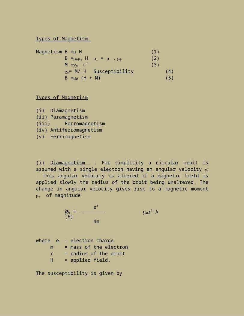
hardnable alloys disappears. Examples of dispersion strengthen composites are: aluminium-aluminium oxides systems having the dispersed particles of Al2 O3 of 0.1- 0.2 and nickel - 3 volume % Thoria (ThO2) known as TD-nickel.

B. Fiber reinforced Composites

The most important Fiber reinforced Composites are those produced by using fibers of fine whiskers. As a matrix there may be metal or alloy, plastic or ceramic. Fibers may also be metals, ceramics or plastics. The importance of fiber reinforced composites is that the tensile strength of fiber is usually greater that for bulk material.

The matrix binds the fibers together and protects them from mechanical and chemical damage that might occur by abrasion of their surface or by chemical effect of some extraneous matter. Also, the matrix separates the individual fibers and prevent a brittle cracks that passes completely across a section of composites. There are two types of fiber reinforced composites:

a) Continuous fibers and b) Discontinuous fibers

a) Continuous fibers :

For Continuous fibers reinforcement the strain in the matrix and in the fiber under a load are initially the same. At low stresses we can assume that both fiber and matrix deform elastically but with increasing stress the matrix may deform plastically while the fiber will still be elastic.

For unidirectional composites of continuous fibers, the strength and the modulus of the composites can be estimated from the following analysis:

We assume that all fibers are identical and are unidirectional, extending through out the composites and that no slippage is permitted at the interface. The strain of the composite must be be equal to the fiber and

Fig. 2 : Distribution of a loads for a continuous fiber reinforced

composite

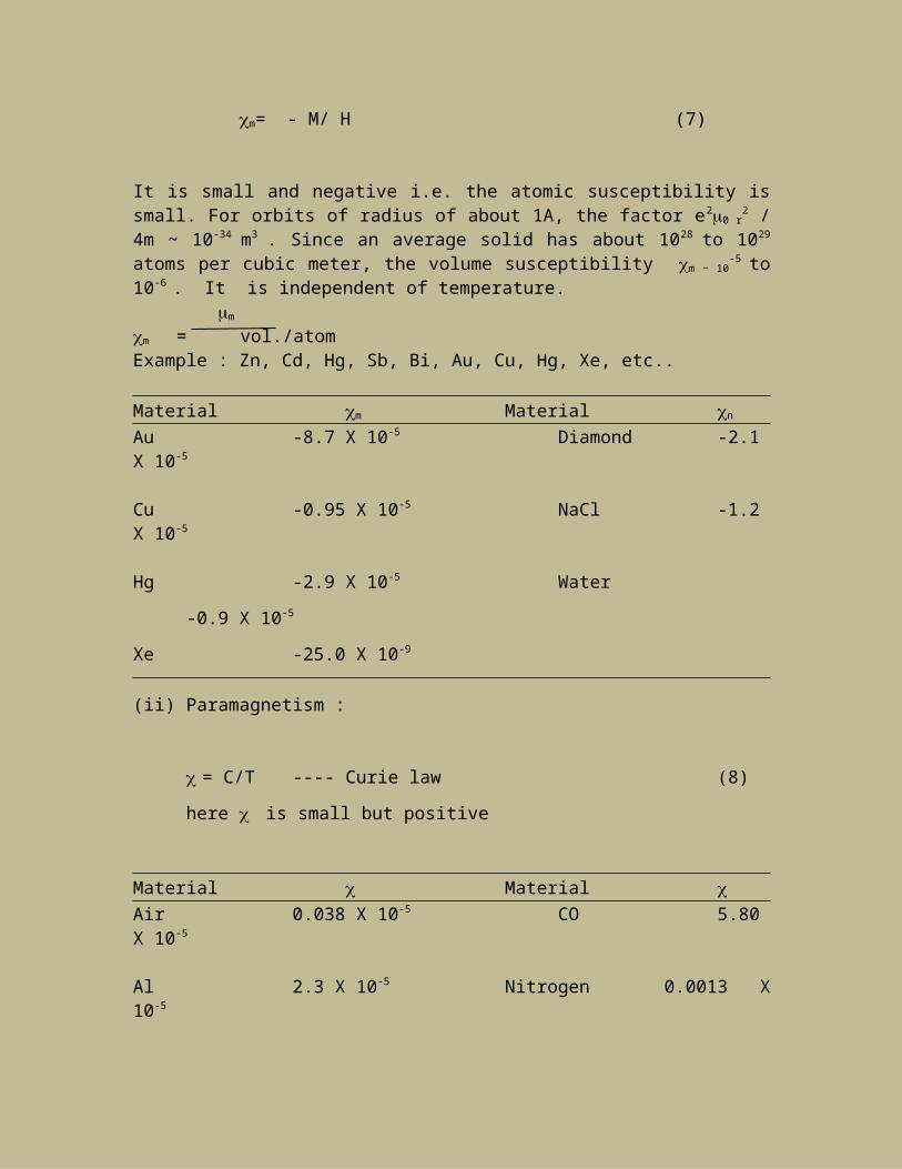
that of the matrix. The load Wc on the composite will be then carried by the fibers Wf and by the matrix Wm so that

(3)

Since the load W= . A, the corresponding stresses s, f and m acting on the respective correctional area Ac, Af and Am will give

c Ac = f Af + m Am (4)rearranging

c = m (Am / Ac) + f (Af / Ac) (5)

Am / Ac can be replaced by the volume fraction m = Vm / Vc and eqn. (5) becomes

c= m m + f f (6)

As ,m+ f = 1 (7)

We get, c=m(1- f) + f f (8)

This equation is valid only for the linear elastic region of the stress-strain curve.

Since the strains on the components are equal (c = m = f), we can write

Ecc = Em m (1- f) + Ef f f (9)

Ec = Em m + Er r (10)where

m= (1- f)The ratio of the load carried by the fibers to that load carried by the matrix is

For effective reinforcement there must be certain minimum volumetric fraction of fibers so that min= < < max.

Illustrative Problem:

(11)

A continuous glass fiber reinforced epoxy, composite is produced using 65% volume of “E” glass fibers having at 250 C Young Modulus Ef = 10.5 X 106 psi, fracture stress f = 500,000 psi and the epoxy resin which on hardening , shows modulus Em = 2.0X 106 psi and tensile strength of 9000 psi. Estimate the longitudinal modulus of the composite and its tensile strength. What fraction of the load will be carried out by the fiber ?

Solution : From eqn. (10)

Ec = Em m + Er r= 2.0 X 106 (1 – 0.65) + 10.5 X 106 X 0.65

= 7.525 X 106 psi.c=f f + m(1- f)

c = 9,000 X 0.35 + 500,000 X 0.65 = 328,150 psi.

From equation (11) on rearranging we get,

Thus 0.91 of the load will be carried out by the fiber and the weakness of the plastic matrix is relatively unimportant.

b) Discontinuous fibers : Most practical composites that are being developed for engineering

applications contain discontinuous fibers. Since fibers do not span the whole length of the specimen, the bond between the matrix and the fiber is broken at the fiber’s ends, which are carrying less strain than the middle part of the fiber. Thus strain in a discontinuous fiber will vary along its length as shown in Fig. below . The average stress of the continuous fiber is then less than the ultimate fiber stress, f .

The Fermi-Dirac Distribution

According to the band theory, the motion of electrons under external electric field is possible only for electrons located in partially filled energy bands.

The energy distribution of gas molecules is controlled by the Maxwell Boltzmann distribution law. This law is no longer applicable to a group of electrons in the atoms whose energy distribution must also obey the Pauli Exclusion Principle ; furthermore, the electrons in metals are in a much greater concentration (about 104 ) than the molecules in ordinary gas . The probability functions that describes the thermal behavior of electrons in atoms is given by Fermi as

(E) = 1 / (e(E - Ef)/kT+1 ) (1)

Where is the Fermi function determining the probability that an energy level E is occupied by an electron, Ef is the Fermi energy or the Fermi level K is the Boltzmann constant, and T is the absolute temperature.The Fermi energy, Ef in a metal represents the kinetic energy of the electrons having the maximum energy level that some electrons can attain. At absolute zero, the Fermi dirac distribution law requires that the Fermi function (E) will have the value 1 or 0. Thus at T = 0 K, (E) = 1 and E < Ef. At temperature greater than 0 K , f(E) changes from one to zero over an energy range of about kT value . At E - E f (E) is equal to one half. If E - Ef >>kT , the exponential term e(E - Ef)/kT in the denominator equation (1) becomes very large compared to unity and we can write

(E) = e(E - Ef)/kT (2)

Equation (2) indicates the probability of occupation of the energy states will vary exponentially following the classical Maxwell – Boltzmann distribution . For electron energy below the Fermi level, Ef – E >> kT , and equation (1) can be approximated as (E) 1 - e(E - Ef)/kT (3)

indicating the probability of occupation of the energy band is nearly unity.Actually, the state densities across the energy band are not uniform and their population density, N(E) is the greatest in the center of the band . Then the number of electrons n e, can be evaluated by integrating the product of the density of state N(E) and the probability of their occupation (E), over the band energy range. Thus for metals

(4)

The energy distribution in the conduction zone extends over several electron volts and it is about 5 eV for some metals at absolute zero. Thus only a small fraction of the electrons in the energy band can be excited above the Fermi level, and only those within an energy range of the order of kT can be excited thermally.

Conductivity

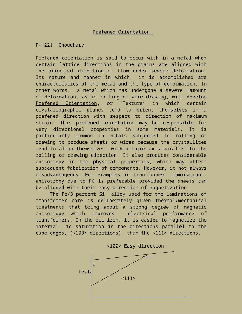
In most cases the electrical conductivity of solids caused by the flow of electron charge carriers under applied electric field, , can be simply represented by Ohm’s law :

J = (5)

Where J is the electric current density, and is the proportionality constant known as electrical conductivity. The electrical density J is defined as the number of electric charges transported through a unit area in a unit time. Since the number of electrons passing through a unit area in a unit time is ,

(6)

where n is the number of electrons per unit volume and d is the average drift velocity of the electrons attained under the electric field. The drift velocity is the average velocity acquired by a carrier in an applied electric field, determined by the value of the field and the amount of scattering of electrons. Combining eqns. (5) and (6) we get,

(7)

Defining the ratio d/ as the mobility of an electric charge ,

= (d / ) (8)We get

= ne (9)

Semiconductivity

In a perfect crystal lattice as , for example, in that of silicon, all four valance electrons are tied in place, forming covalent bonds. The energies of the valance electrons that binds the crystals together lie in the highest filled energy band, called the valance band. The empty band above, called the conduction band, is separated from the valance bond by an energy gap, Eg . The magnitude of the energy gap, or width of the forbidden energy zone, is characteristic of the lattice alone and varies widely for different crystals . The transfer of electron from the valence bond.