MAT 211 Introduction to Business Statistics I Lecture Notes

MAT 211Introduction to Business Statistics I

Lecture Notes

Muhammad El-TahaDepartment of Mathematics and Statistics

University of Southern Maine96 Falmouth Street

Portland, ME 04104-9300

MAT 211, Spring 97, revised Fall 97,revised Spring 98

MAT 211

Introduction to Business Statistics I

Course Content

Topic 1: Data Analysis

Topic 2: Probability

Topic 3: Random Variables and Discrete Distributions

Topic 4: Continuous Probability Distributions

Topic 5: Sampling Distributions

Topic 6: Point and Interval Estimation

1

Contents

1 Data Analysis 4

1 Introduction . . . . . . . . . . . . . . . . . . . . . . . . . . . . . . . . . . 4

2 Graphical Methods . . . . . . . . . . . . . . . . . . . . . . . . . . . . . . 6

3 Numerical methods . . . . . . . . . . . . . . . . . . . . . . . . . . . . . . 8

4 Percentiles . . . . . . . . . . . . . . . . . . . . . . . . . . . . . . . . . . . 15

5 Sample Mean and Variance

For Grouped Data . . . . . . . . . . . . . . . . . . . . . . . . . . . . . . 16

6 z-score . . . . . . . . . . . . . . . . . . . . . . . . . . . . . . . . . . . . . 16

2 Probability 21

1 Sample Space and Events . . . . . . . . . . . . . . . . . . . . . . . . . . 21

2 Probability of an event . . . . . . . . . . . . . . . . . . . . . . . . . . . . 22

3 Laws of Probability . . . . . . . . . . . . . . . . . . . . . . . . . . . . . . 24

4 Counting Sample Points . . . . . . . . . . . . . . . . . . . . . . . . . . . 27

5 Random Sampling . . . . . . . . . . . . . . . . . . . . . . . . . . . . . . 29

6 Modeling Uncertainty . . . . . . . . . . . . . . . . . . . . . . . . . . . . . 29

3 Discrete Random Variables 34

1 Random Variables . . . . . . . . . . . . . . . . . . . . . . . . . . . . . . . 34

2 Expected Value and Variance . . . . . . . . . . . . . . . . . . . . . . . . 36

3 Discrete Distributions . . . . . . . . . . . . . . . . . . . . . . . . . . . . . 37

4 Markov Chains . . . . . . . . . . . . . . . . . . . . . . . . . . . . . . . . 39

4 Continuous Distributions 47

1 Introduction . . . . . . . . . . . . . . . . . . . . . . . . . . . . . . . . . . 47

2 The Normal Distribution . . . . . . . . . . . . . . . . . . . . . . . . . . . 47

3 Uniform: U[a,b] . . . . . . . . . . . . . . . . . . . . . . . . . . . . . . . . 50

4 Exponential . . . . . . . . . . . . . . . . . . . . . . . . . . . . . . . . . . 51

2

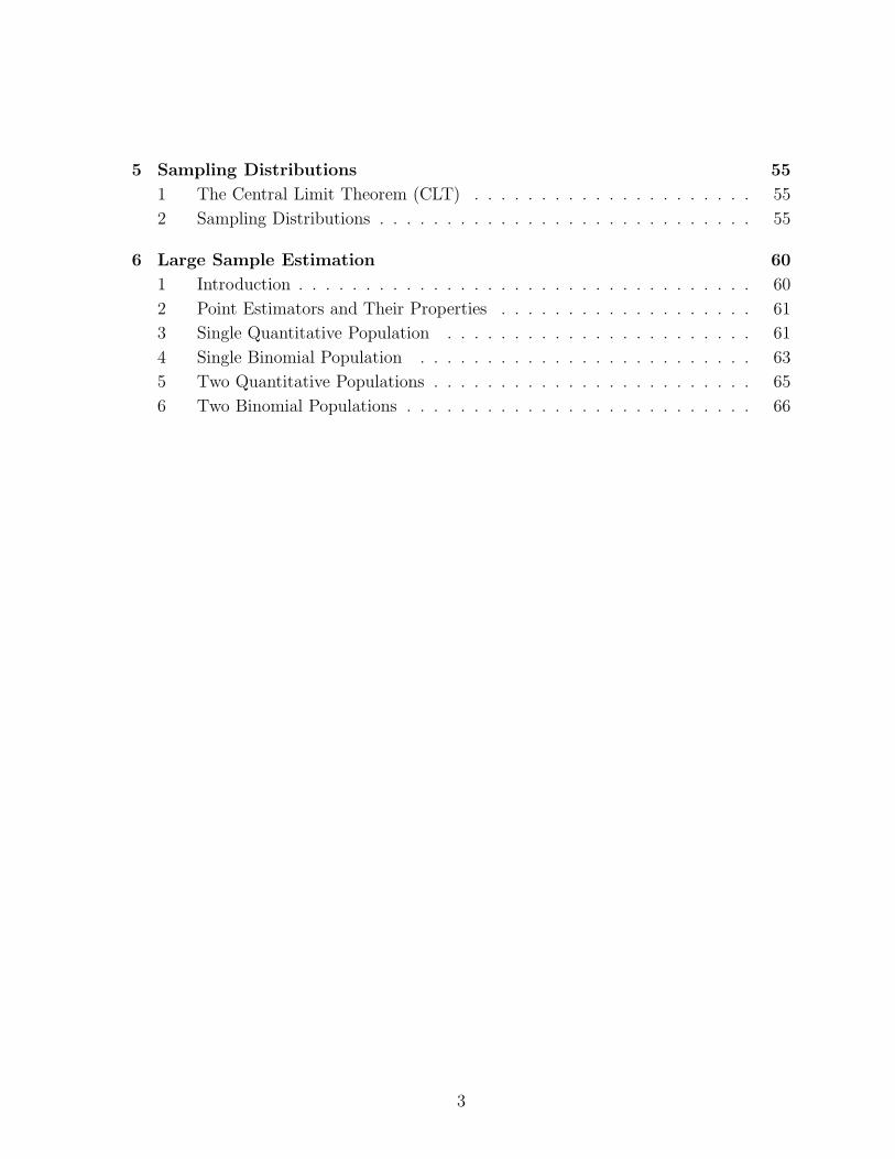
5 Sampling Distributions 55

1 The Central Limit Theorem (CLT) . . . . . . . . . . . . . . . . . . . . . 55

2 Sampling Distributions . . . . . . . . . . . . . . . . . . . . . . . . . . . . 55

6 Large Sample Estimation 60

1 Introduction . . . . . . . . . . . . . . . . . . . . . . . . . . . . . . . . . . 60

2 Point Estimators and Their Properties . . . . . . . . . . . . . . . . . . . 61

3 Single Quantitative Population . . . . . . . . . . . . . . . . . . . . . . . 61

4 Single Binomial Population . . . . . . . . . . . . . . . . . . . . . . . . . 63

5 Two Quantitative Populations . . . . . . . . . . . . . . . . . . . . . . . . 65

6 Two Binomial Populations . . . . . . . . . . . . . . . . . . . . . . . . . . 66

3

Chapter 1

Data Analysis

Chapter Content.

Introduction

Statistical Problems

Descriptive Statistics

Graphical Methods

Frequency Distributions (Histograms)

Other Methods

Numerical methods

Measures of Central Tendency

Measures of Variability

Empirical Rule

Percentiles

1 Introduction

Statistical Problems

1. A market analyst wants to know the effectiveness of a new diet.

2. A pharmaceutical Co. wants to know if a new drug is superior to already existing

drugs, or possible side effects.

3. How fuel efficient a certain car model is?

4. Is there any relationship between your GPA and employment opportunities.

5. If you answer all questions on a (T,F) (or multiple choice) examination completely

randomly, what are your chances of passing?

6. What is the effect of package designs on sales.

4

7. How to interpret polls. How many individuals you need to sample for your infer-

ences to be acceptable? What is meant by the margin of error?

8. What is the effect of market strategy on market share?

9. How to pick the stocks to invest in?

I. Definitions

Probability: A game of chance

Statistics: Branch of science that deals with data analysis

Course objective: To make decisions in the prescence of uncertainty

Terminology

Data: Any recorded event (e.g. times to assemble a product)

Information: Any aquired data ( e.g. A collection of numbers (data))

Knowledge: Useful data

Population: set of all measurements of interest

(e.g. all registered voters, all freshman students at the university)

Sample: A subset of measurements selected from the population of interest

Variable: A property of an individual population unit (e.g. major, height, weight of

freshman students)

Descriptive Statistics: deals with procedures used to summarize the information con-

tained in a set of measurements.

Inferential Statistics: deals with procedures used to make inferences (predictions)

about a population parameter from information contained in a sample.

Elements of a statistical problem:

(i) A clear definition of the population and variable of interest.

(ii) a design of the experiment or sampling procedure.

(iii) Collection and analysis of data (gathering and summarizing data).

(iv) Procedure for making predictions about the population based on sample infor-

mation.

(v) A measure of “goodness” or reliability for the procedure.

Objective. (better statement)

To make inferences (predictions, decisions) about certain characteristics of a popula-

tion based on information contained in a sample.

Types of data: qualitative vs quantitative OR discrete vs continuous

Descriptive statistics

Graphical vs numerical methods

5

2 Graphical Methods

Frequency and relative frequency distributions (Histograms):

Example

Weight Loss Data

20.5 19.5 15.6 24.1 9.915.4 12.7 5.4 17.0 28.616.9 7.8 23.3 11.8 18.413.4 14.3 19.2 9.2 16.88.8 22.1 20.8 12.6 15.9

Objective: Provide a useful summary of the available information.

Method: Construct a statistical graph called a “histogram” (or frequency distribution)

Weight Loss Data

class bound- tally class rel.aries freq, f freq, f/n

1 5.0-9.0- 3 3/25 (.12)2 9.0-13.0- 5 5/25 (.20)3 13.0-17.0- 7 7/25 (.28)4 17.0-21.0- 6 6/25 (.24)5 21.0-25.0- 3 3/25 (.12)6 25.0-29.0 1 1/25 (.04)

Totals 25 1.00

Let

k = # of classes

max = largest measurement

min = smallest measurement

n = sample size

w = class width

Rule of thumb:

-The number of classes chosen is usually between 5 and 20. (Most of the time between

7 and 13.)

-The more data one has the larger is the number of classes.

6

Formulas:

k = 1 + 3.3log10(n);

w =max−min

k.

Note: w = 28.6−5.46

= 3.87. But we used

w = 29−56

= 4.0 (why?)

Graphs: Graph the frequency and relative frequency distributions.

Exercise. Repeat the above example using 12 and 4 classes respectively. Comment on

the usefulness of each including k = 6.

Steps in Constructing a Frequency Distribution (Histogram)

1. Determine the number of classes

2. Determine the class width

3. Locate class boundaries

4. Proceed as above

Possible shapes of frequency distributions

1. Normal distribution (Bell shape)

2. Exponential

3. Uniform

4. Binomial, Poisson (discrete variables)

Important

-The normal distribution is the most popular, most useful, easiest to handle

- It occurs naturally in practical applications

- It lends itself easily to more in depth analysis

Other Graphical Methods

-Statistical Table: Comparing different populations

- Bar Charts

- Line Charts

- Pie-Charts

- Cheating with Charts

7

3 Numerical methods

Measures of Central Measures of DispersionTendency (Variability)

1. Sample mean 1. Range2. Sample median 2. Mean Absolute Deviation (MAD)3. Sample mode 3. Sample Variance

4. Sample Standard Deviation

I. Measures of Central Tendency

Given a sample of measurements (x1, x2, · · · , xn) where

n = sample sizexi = value of the ith observation in the sample

1. Sample Mean (arithmetic average)

x = x1+x2+···+xn

n

or x =∑

x

n

Example 1: Given a sample of 5 test grades

(90, 95, 80, 60, 75)

then

∑x = 90 + 95 + 80 + 60 + 75 = 400

x =∑

x

n= 400

5= 80.

Example 2: Let x = age of a randomly selected student sample:

(20, 18, 22, 29, 21, 19)

∑x = 20 + 18 + 22 + 29 + 21 + 19 = 129

x =∑

x

n= 129

6= 21.5

2. Sample Median

The median of a sample (data set) is the middle number when the measurements are

arranged in ascending order.

Note:

If n is odd, the median is the middle number

8

If n is even, the median is the average of the middle two numbers.

Example 1: Sample (9, 2, 7, 11, 14), n = 5

Step 1: arrange in ascending order

2, 7, 9, 11, 14

Step 2: med = 9.

Example 2: Sample (9, 2, 7, 11, 6, 14), n = 6

Step 1: 2, 6, 7, 9, 11, 14

Step 2: med = 7+92

= 8.

Remarks:

(i) x is sensitive to extreme values

(ii) the median is insensitive to extreme values (because median is a measure of

location or position).

3. Mode

The mode is the value of x (observation) that occurs with the greatest frequency.

Example: Sample: (9, 2, 7, 11, 14, 7, 2, 7), mode = 7

9

Effect of x, median and mode on relative frequency distribution.

10

II. Measures of Variability

Given: a sample of size nsample: (x1, x2, · · · , xn)

1. Range:

Range = largest measurement - smallest measurementor Range = max - min

Example 1: Sample (90, 85, 65, 75, 70, 95)

Range = max - min = 95-65 = 30

2. Mean Absolute Difference (MAD) (not in textbook)

MAD =

∑ |x− x|n

Example 2: Same sample

x =

∑x

n= 80

x x− x |x− x|90 10 1085 5 565 -15 1575 -5 570 -10 1095 15 15

Totals 480 0 60

MAD =

∑ |x− x|n

=60

6= 10.

Remarks:

(i) MAD is a good measure of variability

(ii) It is difficult for mathematical manipulations

3. Sample Variance, s2

s2 =

∑(x− x)2

n− 1

4. Sample Standard Deviation, s

11

s =√s2

or s =

√∑(x−x)2

n−1

Example: Same sample as before (x = 80)

x x− x (x− x)2

90 10 10085 5 2565 -15 22575 -5 2570 -10 10095 15 225

Totals 480 0 700

Therefore

x =

∑x

n=

480

6= 80

s2 =

∑(x− x)2

n− 1=

700

5= 140

s =√s2 =

√140 = 11.83

Shortcut Formula for Calculating s2 and s

s2 =

∑x2 − (

∑x)

2

n

n− 1

s =

√√√√√∑x2 − (∑

x)2

n

n− 1

(or s =√s2).

Example: Same sample

12

x x2

90 810085 722565 422575 562570 490095 9025

Totals 480 39,100

s2 =

∑x2 − (

∑x)

2

n

n− 1=

39, 100− (480)2

6

5

=39, 100− 38, 400

5=

700

5= 140

s =√s2 =

√140 = 11.83.

Numerical methods(Summary)

Data: {x1, x2, · · · , xn}(i) Measures of central tendency

Sample mean: x =∑

xi

n

Sample median: the middle number when the measurements are arranged in ascending

order

Sample mode: most frequently occurring value

(ii) Measures of variability

Range: r = max−min

Sample Variance: s2 =∑

(xi−x)2

n−1

Sample standard deviation: s=√s2

Exercise: Find all the measures of central tendency and measures of variability for the

weight loss example.

Graphical Interpretation of the Variance:

Finite Populations

Let N = population size.

Data: {x1, x2, · · · , xN}Population mean: µ =

∑xi

N

Population variance:

σ2 =

∑(xi − µ)2

N

13

Population standard deviation: σ =√σ2, i.e.

σ =

√∑(xi − µ)2

N

Population parameters vs sample statistics.

Sample statistics: x, s2, s.

Population parameters: µ, σ2, σ.

Practical Significance of the standard deviation

Chebyshev’s Inequality. (Regardless of the shape of frequency distribution)

Given a number k ≥ 1, and a set of measurements x1, x2, . . . , xn, at least (1− 1k2 ) of

the measurements lie within k standard deviations of their sample mean.

Restated. At least (1− 1k2 ) observations lie in the interval (x− ks, x+ ks).

Example. A set of grades has x = 75, s = 6. Then

(i) (k = 1): at least 0% of all grades lie in [69, 81]

(ii) (k = 2): at least 75% of all grades lie in [63, 87]

(iii) (k = 3): at least 88% of all grades lie in [57, 93]

(iv) (k = 4): at least ?% of all grades lie in [?, ?]

(v) (k = 5): at least ?% of all grades lie in [?, ?]

Suppose that you are told that the frequency distribution is bell shaped. Can you

improve the estimates in Chebyshev’s Inequality.

Empirical rule. Given a set of measurements x1, x2, . . . , xn, that is bell shaped. Then

(i) approximately 68% of the measurements lie within one standard deviations of their

sample mean, i.e. (x− s, x+ s)

(ii) approximately 95% of the measurements lie within two standard deviations of

their sample mean, i.e. (x− 2s, x+ 2s)

(iii) at least (almost all) 99% of the measurements lie within three standard deviations

of their sample mean, i.e. (x− 3s, x+ 3s)

Example A data set has x = 75, s = 6. The frequency distribution is known to be

normal (bell shaped). Then

(i) (69, 81) contains approximately 68% of the observations

(ii) (63, 87) contains approximately 95% of the observations

(iii) (57, 93) contains at least 99% (almost all) of the observations

Comments.

(i) Empirical rule works better if sample size is large

(ii) In your calculations always keep 6 significant digits

14

(iii) Approximation: s � range4

(iv) Coefficient of variation (c.v.) = sx

4 Percentiles

Using percentiles is useful if data is badly skewed.

Let x1, x2, . . . , xn be a set of measurements arranged in increasing order.

Definition. Let 0 < p < 100. The pth percentile is a number x such that p% of all

measurements fall below the pth percentile and (100− p)% fall above it.

Example. Data: 2, 5, 8, 10, 11, 14, 17, 20.

(i) Find the 30th percentile.

Solution.

(S1) position = .3(n+ 1) = .3(9) = 2.7

(S2) 30th percentile = 5 + .7(8− 5) = 5 + 2.1 = 7.1

Special Cases.

1. Lower Quartile (25th percentile)

Example.

(S1) position = .25(n+ 1) = .25(9) = 2.25

(S2) Q1 = 5 + .25(8− 5) = 5 + .75 = 5.75

2. Median (50th percentile)

Example.

(S1) position = .5(n+ 1) = .5(9) = 4.5

(S2) median: Q2 = 10 + .5(11− 10) = 10.5

3. Upper Quartile (75th percentile)

Example.

(S1) position = .75(n+ 1) = .75(9) = 6.75

(S2) Q3 = 14 + .75(17− 14) = 16.25

Interquartiles.

IQ = Q3 −Q1

Exercise. Find the interquartile (IQ) in the above example.

15

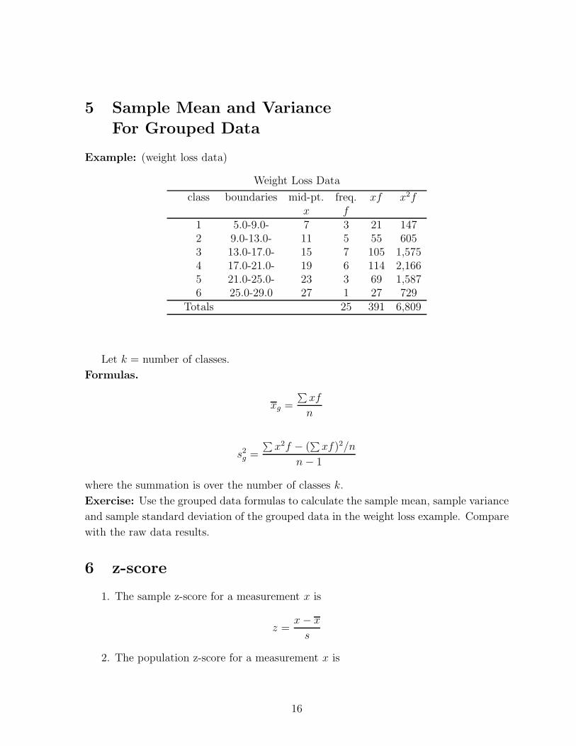
5 Sample Mean and Variance

For Grouped Data

Example: (weight loss data)

Weight Loss Data

class boundaries mid-pt. freq. xf x2fx f

1 5.0-9.0- 7 3 21 1472 9.0-13.0- 11 5 55 6053 13.0-17.0- 15 7 105 1,5754 17.0-21.0- 19 6 114 2,1665 21.0-25.0- 23 3 69 1,5876 25.0-29.0 27 1 27 729

Totals 25 391 6,809

Let k = number of classes.

Formulas.

xg =

∑xf

n

s2g =

∑x2f − (

∑xf)2/n

n− 1

where the summation is over the number of classes k.

Exercise: Use the grouped data formulas to calculate the sample mean, sample variance

and sample standard deviation of the grouped data in the weight loss example. Compare

with the raw data results.

6 z-score

1. The sample z-score for a measurement x is

z =x− x

s

2. The population z-score for a measurement x is

16

z =x− µ

σ

Example. A set of grades has x = 75, s = 6. Suppose your score is 85. What is your

relative standing, (i.e. how many standard deviations, s, above (below) the mean your

score is)?

Answer.

z =x− x

s=

85− 75

6= 1.66

standard deviations above average.

Review Exercises: Data Analysis

Please show all work. No credit for a correct final answer without a valid argu-

ment. Use the formula, substitution, answer method whenever possible. Show your work

graphically in all relevant questions.

1. (Fluoride Problem) The regulation board of health in a particular state specify

that the fluoride level must not exceed 1.5 ppm (parts per million). The 25 measurements

below represent the fluoride level for a sample of 25 days. Although fluoride levels are

measured more than once per day, these data represent the early morning readings for

the 25 days sampled.

.75 .86 .84 .85 .97

.94 .89 .84 .83 .89

.88 .78 .77 .76 .82

.71 .92 1.05 .94 .83

.81 .85 .97 .93 .79

(i) Show that x = .8588, s2 = .0065, s = .0803.

(ii) Find the range, R.

(iii) Using k = 7 classes, find the width, w, of each class interval.

(iv) Locate class boundaries

(v) Construct the frequency and relative frequency distributions for the data.

17

class frequency relative frequency.70-.75-.75-.80-.80-.85-.85-.90-.90-.95-.95-1.00-1.00-1.05Totals

(vi) Graph the frequency and relative frequency distributions and state your conclu-

sions. (Vertical axis must be clearly labeled)

2. Given the following data set (weight loss per week)

(9, 2, 5, 8, 4, 5)

(i) Find the sample mean.

(ii) Find the sample median.

(iii) Find the sample mode.

(iv) Find the sample range.

(v) Find the mean absolute difference.

(vi) Find the sample variance using the defining formula.

(vii) Find the sample variance using the short-cut formula.

(viii) Find the sample standard deviation.

(ix) Find the first and third quartiles, Q1 and Q3.

(x) Repeat (i)-(ix) for the data set (21, 24, 15, 16, 24).

Answers: x = 5.5, med =5, mode =5 range = 7, MAD=2, ss, 6.7, s = 2.588, Q− 3 =

8.25.

3. Grades for 50 students from a previous MAT test are summarized below.

class frequency, f xf x2f40 -50- 450 -60- 660-70- 1070-80- 1580-90- 1090-100 5Totals

18

(i) Complete all entries in the table.

(ii) Graph the frequency distribution. (Vertical axis must be clearly labeled)

(iii) Find the sample mean for the grouped data

(iv) Find the sample variance and standard deviation for the grouped data.

Answers: Σxf = 3610,Σx2f = 270, 250, x = 72.2, s2 = 196, s = 14.

4. Refer to the raw data in the fluoride problem.

(i) Find the sample mean and standard deviation for the raw data.

(ii) Find the sample mean and standard deviation for the grouped data.

(iii) Compare the answers in (i) and (ii).

Answers: Σxf = 21.475,Σx2f = 18.58, xg =, sg = .0745.

5. Suppose that the mean of a population is 30. Assume the standard deviation is

known to be 4 and that the frequency distribution is known to be bell-shaped.

(i) Approximately what percentage of measurements fall in the interval (22, 34)

(ii) Approximately what percentage of measurements fall in the interval (µ, µ+ 2σ)

(iii) Find the interval around the mean that contains 68% of measurements

(iv)Find the interval around the mean that contains 95% of measurements

6. Refer to the data in the fluoride problem. Suppose that the relative frequency

distribution is bell-shaped. Using the empirical rule

(i) find the interval around the mean that contains 99.6% of measurements.

(ii) find the percentage of measurements fall in the interval (µ+ 2σ,∞)

7. (4 pts.) Answer by True of False . (Circle your choice).

T F (i) The median is insensitive to extreme values.

T F (ii) The mean is insensitive to extreme values.

T F (iii) For a positively skewed frequency distribution, the mean is larger than the

median.

T F (iv) The variance is equal to the square of the standard deviation.

T F (v) Numerical descriptive measures computed from sample measurements are

called parameters.

T F (vi) The number of students attending a Mathematics lecture on any given day

is a discrete variable.

19

T F (vii) The median is a better measure of central tendency than the mean when a

distribution is badly skewed.

T F (viii) Although we may have a large mass of data, statistical techniques allow us

to adequately describe and summarize the data with an average.

T F (ix) A sample is a subset of the population.

T F (x) A statistic is a number that describes a population characteristic.

T F (xi) A parameter is a number that describes a sample characteristic.

T F (xii) A population is a subset of the sample.

T F (xiii) A population is the complete collection of items under study.

20

Chapter 2

Probability

Contents.

Sample Space and Events

Probability of an Event

Equally Likely Outcomes

Conditional Probability and Independence

Laws of Probability

Counting Sample Points

Random Sampling

1 Sample Space and Events

Definitions

Random experiment: involves obtaining observations of some kind

Examples Toss of a coin, throw a die, polling, inspecting an assembly line, counting

arrivals at emergency room, etc.

Population: Set of all possible observations. Conceptually, a population could be gen-

erated by repeating an experiment indefinitely.

Outcome of an experiment:

Elementary event (simple event): one possible outcome of an experiment

Event (Compound event): One or more possible outcomes of a random experiment

Sample space: the set of all sample points (simple events) for an experiment is called

a sample space; or set of all possible outcomes for an experiment

Notation.

Sample space : S

21

Sample point: E1, E2, . . . etc.

Event: A,B,C,D,E etc. (any capital letter).

Venn diagram:

Example.

S = {E1, E2, . . . , E6}.That is S = {1, 2, 3, 4, 5, 6}. We may think of S as representation of possible outcomes

of a throw of a die.

More definitions

Union, Intersection and Complementation

Given A and B two events in a sample space S.

1. The union of A and B, A ∪ B, is the event containing all sample points in either

A or B or both. Sometimes we use AorB for union.

2. The intersection of A and B, A∩B, is the event containing all sample points that

are both in A and B. Sometimes we use AB or AandB for intersection.

3. The complement of A, Ac, is the event containing all sample points that are not in

A. Sometimes we use notA or A for complement.

Mutually Exclusive Events (Disjoint Events) Two events are said to be mutually

exclusive (or disjoint) if their intersection is empty. (i.e. A ∩ B = φ).

Example Suppose S = {E1, E2, . . . , E6}. LetA = {E1, E3, E5};B = {E1, E2, E3}. Then(i)A ∪B = {E1, E2, E3, E5}.(ii) AB = {E1, E3}.(iii) Ac = {E2, E4, E6}; Bc = {E4, E5, E6};(iv) A and B are not mutually exclusive (why?)

(v) Give two events in S that are mutually exclusive.

2 Probability of an event

Relative Frequency Definition If an experiment is repeated a large number, n, of

times and the event A is observed nA times, the probability of A is

P (A) � nA

n

Interpretation

n = # of trials of an experiment

22

nA = frequency of the event AnA

n= relative frequency of A

P (A) � nA

nif n is large enough.

(In fact, P (A) = limn→∞ nA

n.)

Conceptual Definition of Probability

Consider a random experiment whose sample space is S with sample points E1, E2, . . . ,.

For each event Ei of the sample space S define a number P (E) that satisfies the following

three conditions:

(i) 0 ≤ P (Ei) ≤ 1 for all i

(ii) P (S) = 1

(iii) (Additive property) ∑S

P (Ei) = 1,

where the summation is over all sample points in S.

We refer to P (Ei) as the probability of the Ei.

Definition The probability of any event A is equal to the sum of the probabilities of the

sample points in A.

Example. Let S = {E1, . . . , E10}. It is known that P (Ei) = 1/20, i = 1, . . . , 6 and

P (Ei) = 1/5, i = 7, 8, 9 and P (E10) = 2/20. In tabular form, we have

Ei E1 E2 E3 E4 E5 E6 E7 E8 E9 E10

p(Ei) 1/20 1/20 1/20 1/20 1/20 1/20 1/5 1/5 1/5 1/10

Question: Calculate P (A) where A = {Ei, i ≥ 6}.A:

P (A) = P (E6) + P (E7) + P (E8) + P (E9) + P (E10)

= 1/20 + 1/5 + 1/5 + 1/5 + 1/10 = 0.75

Steps in calculating probabilities of events

1. Define the experiment

2. List all simple events

3. Assign probabilities to simple events

4. Determine the simple events that constitute an event

5. Add up the simple events’ probabilities to obtain the probability of the event

23

Example Calculate the probability of observing one H in a toss of two fair coins.

Solution.

S = {HH,HT, TH, TT}A = {HT, TH}P (A) = 0.5

Interpretations of Probability

(i) In real world applications one observes (measures) relative frequencies, one cannot

measure probabilities. However, one can estimate probabilities.

(ii) At the conceptual level we assign probabilities to events. The assignment, how-

ever, should make sense. (e.g. P(H)=.5, P(T)=.5 in a toss of a fair coin).

(iii) In some cases probabilities can be a measure of belief (subjective probability).

This measure of belief should however satisfy the axioms.

(iv) Typically, we would like to assign probabilities to simple events directly; then use

the laws of probability to calculate the probabilities of compound events.

Equally Likely Outcomes

The equally likely probability P defined on a finite sample space S = {E1, . . . , EN},assigns the same probability P (Ei) = 1/N for all Ei.

In this case, for any event A

P (A) =NA

N=

sample points in A

sample points in S=

#(A)

#(S)

where N is the number of the sample points in S and NA is the number of the sample

points in A.

Example. Toss a fair coin 3 times.

(i) List all the sample points in the sample space

Solution: S = {HHH, · · ·TTT} (Complete this)

(ii) Find the probability of observing exactly two heads, at most one head.

3 Laws of Probability

Conditional Probability

The conditional probability of the event A given that event B has occurred is denoted

by P (A|B). Then

P (A|B) =P (A ∩B)

P (B)

24

provided P (B) > 0. Similarly,

P (B|A) =P (A ∩B)

P (A)

Independent Events

Definitions. (i) Two events A and B are said to be independent if

P (A ∩ B) = P (A)P (B).

(ii) Two events A and B that are not independent are said to be dependent.

Remarks. (i) If A and B are independent, then

P (A|B) = P (A) and P (B|A) = P (B).

(ii) If A is independent of B then B is independent of A.

Probability Laws

Complementation law:

P (A) = 1− P (Ac)

Additive law:

P (A ∪ B) = P (A) + P (B)− P (A ∩B)

Moreover, if A and B are mutually exclusive, then P (AB) = 0 and

P (A ∪B) = P (A) + P (B)

Multiplicative law (Product rule)

P (A ∩ B) = P (A|B)P (B)

= P (B|A)P (A)

Moreover, if A and B are independent

P (AB) = P (A)P (B)

Example Let S = {E1, E2, . . . , E6}; A = {E1, E3, E5}; B = {E1, E2, E3}; C = {E2, E4, E6};D =

{E6}. Suppose that all elementary events are equally likely.

(i) What does it mean that all elementary events are equally likely?

(ii) Use the complementation rule to find P (Ac).

(iii) Find P (A|B) and P (B|A)

(iv) Find P (D) and P (D|C)

25

(v) Are A and B independent? Are C and D independent?

(vi) Find P (A ∩B) and P (A ∪ B).

Law of total probability Let the B,Bc be complementary events and let A denote an

arbitrary event. Then

P (A) = P (A ∩B) + P (A ∩ Bc) ,

or

P (A) = P (A|B)P (B) + P (A|Bc)P (Bc).

Bayes’ Law

Let the B,Bc be complementary events and let A denote an arbitrary event. Then

P (B|A) =P (AB)

P (A)=

P (A|B)P (B)

P (A|B)P (B) + P (A|Bc)P (Bc).

Remarks.

(i) The events of interest here areB,Bc, P (B) and P (Bc) are called prior probabilities,

and

(ii) P (B|A) and P (Bc|A) are called posterior (revised) probabilities.

(ii) Bayes’ Law is important in several fields of applications.

Example 1. A laboratory blood test is 95 percent effective in detecting a certain disease

when it is, in fact, present. However, the test also yields a “false positive” results for

1 percent of healthy persons tested. (That is, if a healthy person is tested, then, with

probability 0.01, the test result will imply he or she has the disease.) If 0.5 percent of

the population actually has the disease, what is the probability a person has the disease

given that the test result is positive?

Solution Let D be the event that the tested person has the disease and E the event

that the test result is positive. The desired probability P (D|E) is obtained by

P (D|E) =P (D ∩E)

P (E)

=P (E|D)P (D)

P (E|D)P (D) + P (E|Dc)P (Dc)

=(.95)(.005)

(.95)(.005) + (.01)(.995)

=95

294� .323.

26

Thus only 32 percent of those persons whose test results are positive actually have the

disease.

Probabilities in Tabulated Form

4 Counting Sample Points

Is it always necessary to list all sample points in S?

Coin Tosses

Coins sample-points Coins sample-points1 2 2 43 8 4 165 32 6 6410 1024 20 1,048,57630 � 109 40 � 1012

50 � 1015 64 � 1019

Note that 230 � 109 = one billion, 240 � 1012 = one thousand billion, 250 � 1015 =

one trillion.

RECALL: P (A) = nA

n, so for some applications we need to find n, nA where n and

nA are the number of points in S and A respectively.

Basic principle of counting: mn rule

Suppose that two experiments are to be performed. Then if experiment 1 can result

in any one of m possible outcomes and if, for each outcome of experiment 1, there are n

possible outcomes of experiment 2, then together there are mn possible outcomes of the

two experiments.

Examples.

(i) Toss two coins: mn = 2× 2 = 4

(ii) Throw two dice: mn = 6× 6 = 36

(iii) A small community consists of 10 men, each of whom has 3 sons. If one man

and one of his sons are to be chosen as father and son of the year, how many different

choices are possible?

Solution: Let the choice of the man as the outcome of the first experiment and the

subsequent choice of one of his sons as the outcome of the second experiment, we see,

from the basic principle, that there are 10× 3 = 30 possible choices.

Generalized basic principle of counting

27

If r experiments that are to be performed are such that the first one may result in

any of n1 possible outcomes, and if for each of these n1 possible outcomes there are n2

possible outcomes of the second experiment, and if for each of the possible outcomes of

the first two experiments there are n3 possible outcomes of the third experiment, and if,

. . ., then there are a total of n1 · n2 · · ·nr possible outcomes of the r experiments.

Examples

(i) There are 5 routes available between A and B; 4 between B and C; and 7 between

C and D. What is the total number of available routes between A and D?

Solution: The total number of available routes is mnt = 5.4.7 = 140.

(ii) A college planning committee consists of 3 freshmen, 4 sophomores, 5 juniors,

and 2 seniors. A subcommittee of 4, consisting of 1 individual from each class, is to be

chosen. How many different subcommittees are possible?

Solution: It follows from the generalized principle of counting that there are 3·4·5·2 =

120 possible subcommittees.

(iii) How many different 7−place license plates are possible if the first 3 places are to

be occupied by letters and the final 4 by numbers?

Solution: It follows from the generalized principle of counting that there are 26 · 26 ·26 · 10 · 10 · 10 · 10 = 175, 760, 000 possible license plates.

(iv) In (iii), how many license plates would be possible if repetition among letters or

numbers were prohibited?

Solution: In this case there would be 26 · 25 · 24 · 10 · 9 · 8 · 7 = 78, 624, 000 possible

license plates.

Permutations: (Ordered arrangements)

The number of ways of ordering n distinct objects taken r at a time (order is impor-

tant) is given by

n!

(n− r)!= n(n− 1)(n− 2) · · · (n− r + 1)

Examples

(i) In how many ways can you arrange the letters a, b and c. List all arrangements.

Answer: There are 3! = 6 arrangements or permutations.

(ii) A box contains 10 balls. Balls are selected without replacement one at a time. In

how many different ways can you select 3 balls?

Solution: Note that n = 10, r = 3. Number of different ways is

10 · 9 · 8 = 10!7!

= 720,

28

(which is equal to n!(n−r)!

).

Combinations

For r ≤ n, we define

(n

r

)=

n!

(n− r)!r!

and say that(

nr

)represents the number of possible combinations of n objects taken r at

a time (with no regard to order).

Examples

(i) A committee of 3 is to be formed from a group of 20 people. How many different

committees are possible?

Solution: There are(

203

)= 20!

3!17!= 20.19.18

3.2.1= 1140 possible committees.

(ii) From a group of 5 men and 7 women, how many different committees consisting

of 2 men and 3 women can be formed?

Solution:(

52

) (73

)= 350 possible committees.

5 Random Sampling

Definition. A sample of size n is said to be a random sample if the n elements are selected

in such a way that every possible combination of n elements has an equal probability of

being selected.

In this case the sampling process is called simple random sampling.

Remarks. (i) If n is large, we say the random sample provides an honest representation

of the population.

(ii) For finite populations the number of possible samples of size n is(

Nn

). For instance

the number of possible samples when N = 28 and n = 4 is(

284

)= 20, 475.

(iii) Tables of random numbers may be used to select random samples.

6 Modeling Uncertainty

The purpose of modeling uncertainty (randomness) is to discover the laws of change.

1. Concept of Probability. Even though probability (chance) involves the notion of

change, the laws governing the change may themselves remain fixed as time passes.

Example. Consider a chance experiment: Toss of a coin.

29

Probabilistic Law. In a fair coin tossing experiment the percentage of (H)eads is very

close to 0.5. In the model (abstraction): P (H) = 0.5 exactly.

Why Probabilistic Reasoning?

Example. Toss 5 coins repeatedly and write down the number of heads observed in each

trial. Now, what percentage of trials produce 2 Heads?

answer. Use the Binomial law to show that

P (2Heads) =(5

2

)(0.5)2(1− .5)3

=5!

2!3!(0.5)2(.5)3 = 0.3125

Conclusion. There is no need to carry out this experiment to answer the question.

(Thus saving time and effort).

2. The Interplay Between Probability and Statistics. (Theory versus Application)

(i) Theory is an exact discipline developed from logically defined axioms (conditions).

(ii) Theory is related to physical phenomena only in inexact terms (i.e. approxi-

mately).

(iii) When theory is applied to real problems, it works ( i.e. it makes sense).

Example. A fair die is tossed for a very large number of times. It was observed that

face 6 appeared 1, 500. Estimate how many times the die is tossed.

Answer. 9000 times.

Review Exercises: Probability




1. An experiment consists of tossing 3 fair coins.

(i) List all the elements in the sample space.

(ii) Describe the following events:

A = { observe exactly two heads}B = { Observe at most one tail}C = { Observe at least two heads}D = {Observe exactly one tail}(iii) Find the probabilities of events A,B,C,D.

30

2. Suppose that S = {1, 2, 3, 4, 5, 6} such that P (1) = .1, P (2) = .1,P(3)=.1, P(4)=.2,

P (5) = .2, P (6) = .3.

(i) Find the probability of the event A = {4, 5, 6}.(ii) Find the probability of the complement of A.

(iii) Find the probability of the event B = {even}.(iv) Find the probability of the event C = {odd}.

3. An experiment consists of throwing a fair die.

(i) List all the elements in the sample space.

(ii) Describe the following events:

A = { observe a number larger than 3 }B = { Observe an even number}C = { Observe an odd number}(iii) Find the probabilities of events A,B,C.

(iv) Compare problems 2. and 3.

4. Refer to problem 3. Find

(i) A ∪ B

(ii) A ∩ B

(iii) B ∩ C

(iv) Ac

(v) Cc

(vi) A ∪ C

(vii) A ∩ C

(viii) Find the probabilities in (i)-(vii).

(ix) Refer to problem 2., and answer questions (i)-(viii).

5. The following probability table gives the intersection probabilities for four events

A,B,C and D:

A BC .06 0.31D .55 .08

1.00

(i) Using the definitions, find P (A), P (B), P (C), P (D), P (C|A), P (D|A) and P (C|B).

31

(ii) Find P (Bc).

(iii) Find P (A ∩ B).

(iv) Find P (A ∪B).

(v) Are B and C independent events? Justify your answer.

(vi) Are B and C mutually exclusive events? Justify your answer.

(vii) Are C and D independent events? Justify your answer.

(viii) Are C and D mutually exclusive events? Justify your answer.

6. Use the laws of probability to justify your answers to the following questions:

(i) If P (A ∪ B) = .6, P (A) = .2, and P (B) = .4, are A and B mutually exclusive?

independent?

(ii) If P (A ∪ B) = .65, P (A) = .3, and P (B) = .5, are A and B mutually exclusive?

independent?

(iii) If P (A ∪ B) = .7, P (A) = .4, and P (B) = .5, are A and B mutually exclusive?

independent?

7. Suppose that the following two weather forecasts were reported on two local TV

stations for the same period. First report: The chances of rain are today 30%, tomorrow

40%, both today and tomorrow 20%, either today or tomorrow 60%. Second report: The

chances of rain are today 30%, tomorrow 40%, both today and tomorrow 10%, either

today or tomorrow 60%. Which of the two reports, if any, is more believable? Why? No

credit if answer is not justified. (Hint: Let A and B be the events of rain today and rain

tomorrow.)

8. A box contains five balls, a black (b), white (w), red (r), orange (o), and green (g).

Three balls are to be selected at random.

(i) Find the sample space S (Hint: there is 10 sample points).

S = {bwr, · · ·}(ii) Find the probability of selecting a black ball.

(iii) Find the probability of selecting one black and one red ball.

9. A box contains four black and six white balls.

(i) If a ball is selected at random, what is the probability that it is white? black?

(ii) If two balls are selected without replacement, what is the probability that both

balls are black? both are white? the first is white and the second is black? the first is

black and the second is white? one ball is black?

(iii) Repeat (ii) if the balls are selected with replacement.

32

(Hint: Start by defining the events B1and B − 2 as the first ball is black and the

second ball is black respectively, and by defining the events W1 abd W − 2 as the first

ball is white and the second ball is white respectively. Then use the product rule)

10. Answer by True of False . (Circle your choice).

T F (i) An event is a specific collection of simple events.

T F (ii) The probability of an event can sometimes be negative.

T F (iii) If A and B are mutually exclusive events, then they are also dependent.

T F (iv) The sum of the probabilities of all simple events in the sample space may be

less than 1 depending on circumstances.

T F (v) A random sample of n observations from a population is not likely to provide

a good estimate of a parameter.

T F (vi) A random sample of n observations from a population is one in which every

different subset of size n from the population has an equal probability of being selected.

T F (vii) The probability of an event can sometimes be larger than one.

T F (viii) The probability of an elementary event can never be larger than one half.

T F (ix) Although the probability of an event occurring is .9, the event may not occur

at all in 10 trials.

T F (x) If a random experiment has 5 possible outcomes, then the probability of each

outcome is 1/5.

T F (xi) If two events are independent, the occurrence of one event should not affect

the likelihood of the occurrence of the other event.

33

Chapter 3

Random Variables and DiscreteDistributions

Contents.

Random Variables

Expected Values and Variance

Binomial

Poisson

Hypergeometric

1 Random Variables

The discrete rv arises in situations when the population (or possible outcomes) are

discrete (or qualitative).

Example. Toss a coin 3 times, then

S = {HHH,HHT,HTH,HTT, THH, THT, TTH, TTT}Let the variable of interest, X, be the number of heads observed then relevant events

would be

{X = 0} = {TTT}{X = 1} = {HTT, THT, TTH}{X = 2} = {HHT,HTH, THH}{X = 3} = {HHH}.The relevant question is to find the probability of each these events.

Note that X takes integer values even though the sample space consists of H’s and

T’s.

34

The variable X transforms the problem of calculating probabilities from that of set

theory to calculus.

Definition. A random variable (r.v.) is a rule that assigns a numerical value to each

possible outcome of a random experiment.

Interpretation:

-random: the value of the r.v. is unknown until the outcome is observed

- variable: it takes a numerical value

Notation: We use X, Y , etc. to represent r.v.s.

A Discrete r.v. assigns a finite or countably infinite number of possible values

(e.g. toss a coin, throw a die, etc.)

A Continuous r.v. has a continuum of possible values.

(e.g. height, weight, price, etc.)

Discrete Distributions The probability distribution of a discrete r.v., X, assigns a

probability p(x) for each possible x such that

(i) 0 ≤ p(x) ≤ 1, and

(ii)∑

x p(x) = 1

where the summation is over all possible values of x.

Discrete distributions in tabulated form

Example.

Which of the following defines a probability distribution?

x 0 1 2p(x) 0.30 0.50 0.20

x 0 1 2p(x) 0.60 0.50 -0.10

x -1 1 2p(x) 0.30 0.40 0.20

Remarks. (i) Discrete distributions arise when the r.v. X is discrete (qualitative data)

35

(ii) Continuous distributions arise when the r.v. X is continuous (quantitative data)

Remarks. (i) In data analysis we described a set of data (sample) by dividing it into

classes and calculating relative frequencies.

(ii) In Probability we described a random experiment (population) in terms of events

and probabilities of events.

(iii) Here, we describe a random experiment (population) by using random variables,

and probability distribution functions.

2 Expected Value and Variance

Definition 2.1 The expected value of a discrete rv X is denoted by µ and is defined to

be

µ =∑x

xp(x).

Notation: The expected value of X is also denoted by µ = E[X]; or sometimes µX to

emphasize its dependence on X.

Definition 2.2 If X is a rv with mean µ, then the variance of X is defined by

σ2 =∑x

(x− µ)2p(x)

Notation: Sometimes we use σ2 = V (X) (or σ2X).

Shortcut Formula

σ2 =∑

x2p(x)− µ2

Definition 2.3 If X is a rv with mean µ, then the standard deviation of X, denoted by

σX , (or simply σ) is defined by

σ =√V (X) =

√∑(x− µ)2p(x)

Shortcut Formula

σ =

√∑x2p(x)− µ2

36

3 Discrete Distributions

Binomial.

The binomial experiment (distribution) arises in following situation:

(i) the underlying experiment consists of n independent and identical trials;

(ii) each trial results in one of two possible outcomes, a success or a failure;

(iii) the probability of a success in a single trial is equal to p and remains the same

throughout the experiment; and

(iv) the experimenter is interested in the rv X that counts the number of successes

observed in n trials.

A r.v. X is said to have a binomial distribution with parameters n and p if

p(x) =(n

x

)pxqn−x (x = 0, 1, . . . , n)

where q = 1− p.

Mean: µ = np

Variance: σ2 = npq, σ =√npq

Example: Bernoulli.

A rv X is said to have a Bernoulli distribution with parameter p if

Formula: p(x) = px(1− p)1−x x = 0, 1.

Tabulated form:

x 0 1p(x) 1-p p

Mean: µ = p

Variance: σ2 = pq, σ =√pq

Binomial Tables.

Cumulative probabilities are given in the table.

Example. Suppose X has a binomial distribution with n = 10, p = .4. Find

(i) P (X ≤ 4) = .633

(ii) P (X < 6) = P (X ≤ 5) = .834

(iii) P (X > 4) = 1− P (X ≤ 4) = 1− .633 = .367

(iv) P (X = 5) = P (X ≤ 5)− P (X ≤ 4) = .834− .633 = .201

Exercise: Answer the same question with p = 0.7

37

Poisson.

The Poisson random variable arises when counting the number of events that occur

in an interval of time when the events are occurring at a constant rate; examples include

number of arrivals at an emergency room, number of items demanded from an inventory;

number of items in a batch of a random size.

A rv X is said to have a Poisson distribution with parameter λ > 0 if

p(x) = e−λλx/x!, x = 0, 1, . . . .

Graph.

Mean: µ = λ

Variance: σ2 = λ, σ =√λ

Note: e � 2.71828

Example. Suppose the number of typographical errors on a single page of your book

has a Poisson distribution with parameter λ = 1/2. Calculate the probability that there

is at least one error on this page.

Solution. Letting X denote the number of errors on a single page, we have

P (X ≥ 1) = 1− P (X = 0) = 1− e−0.5 � 0.395

Rule of Thumb. The Poisson distribution provides good approximations to binomial

probabilities when n is large and µ = np is small, preferably with np ≤ 7.

Example. Suppose that the probability that an item produced by a certain machine

will be defective is 0.1. Find the probability that a sample of of 10 items will contain at

most 1 defective item.

Solution. Using the binomial distribution, the desired probability is

P (X ≤ 1) = p(0) + p(1) =

(10

0

)(0.1)0(0.9)10 +

(10

1

)(0.1)1(0.9)9 = 0.7361

Using Poisson approximation, we have λ = np = 1

e−1 + e−1 � 0.7358

which is close to the exact answer.

Hypergeometric.

The hypergeometric distribution arises when one selects a random sample of size n,

without replacement, from a finite population of size N divided into two classes consisting

38

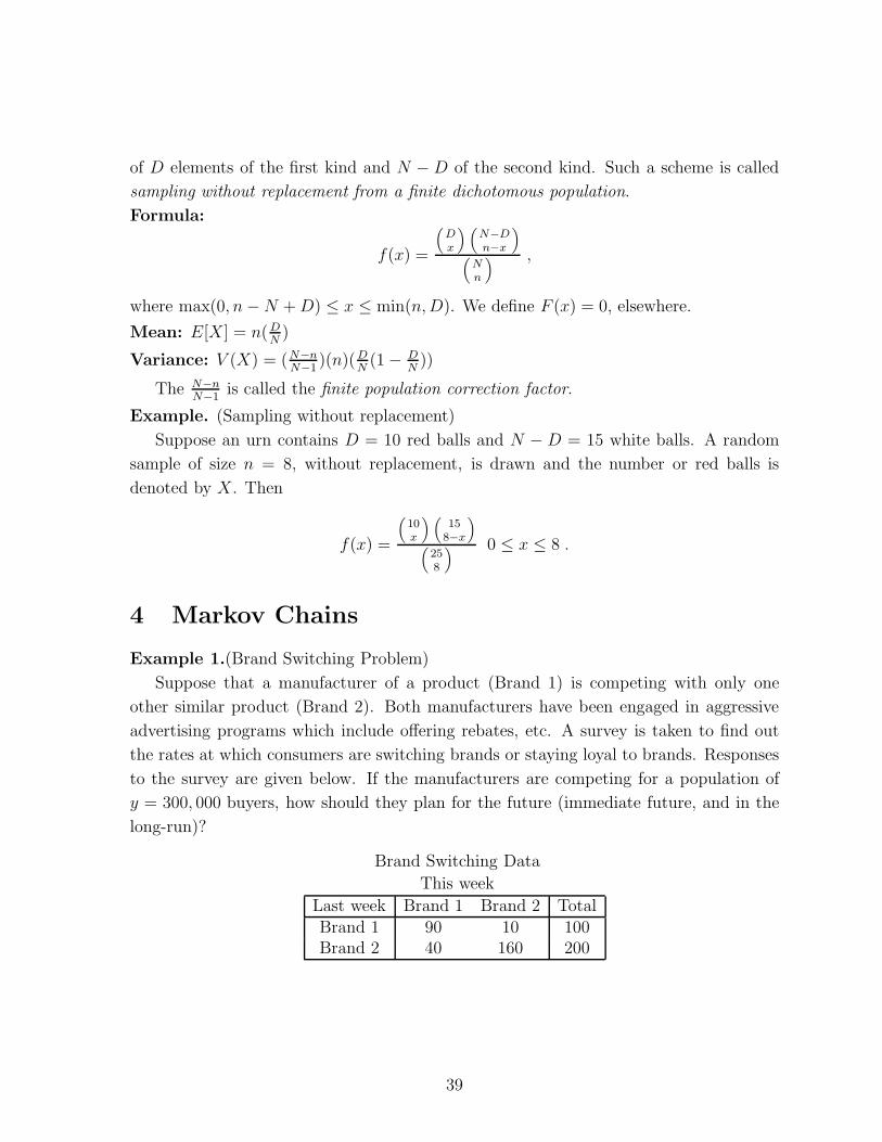
of D elements of the first kind and N − D of the second kind. Such a scheme is called

sampling without replacement from a finite dichotomous population.

Formula:

f(x) =

(Dx

) (N−Dn−x

)(

Nn

) ,

where max(0, n−N +D) ≤ x ≤ min(n,D). We define F (x) = 0, elsewhere.

Mean: E[X] = n(DN)

Variance: V (X) = (N−nN−1

)(n)(DN(1− D

N))

The N−nN−1

is called the finite population correction factor.

Example. (Sampling without replacement)

Suppose an urn contains D = 10 red balls and N − D = 15 white balls. A random

sample of size n = 8, without replacement, is drawn and the number or red balls is

denoted by X. Then

f(x) =

(10x

) (15

8−x

)(

258

) 0 ≤ x ≤ 8 .

4 Markov Chains

Example 1.(Brand Switching Problem)

Suppose that a manufacturer of a product (Brand 1) is competing with only one

other similar product (Brand 2). Both manufacturers have been engaged in aggressive

advertising programs which include offering rebates, etc. A survey is taken to find out

the rates at which consumers are switching brands or staying loyal to brands. Responses

to the survey are given below. If the manufacturers are competing for a population of

y = 300, 000 buyers, how should they plan for the future (immediate future, and in the

long-run)?

Brand Switching Data

This week

Last week Brand 1 Brand 2 TotalBrand 1 90 10 100Brand 2 40 160 200

39

Brand 1 Brand 2Brand 1 90/100 10/100Brand 2 40/200 160/200

So

P =

(0.9 0.10.2 0.8

)

Question 1. suppose that customer behavior is not changed over time. If 1/3 of all

customers purchased B1 this week.

What percentage will purchase B1 next week?

What percentage will purchase B2 next week?

What percentage will purchase B1 two weeks from now?

What percentage will purchase B2 two weeks from now?

Solution: Note that π0 = (1/3, 2/3), then

π1 = (π11, π

12) = (π0

1, π02)P

π1 = (π11, π

12) = (1/3, 2/3)

(0.9 0.10.2 0.8

)= (1.3/3, 1.7/3)

B1 buyers will be 300, 000(1.3/3) = 130, 000

B2 buyers will be 300, 000(1.7/3) = 170, 000.

Two weeks from now: exercise.

Question 2. Determine whether each brand will eventually retain a constant share of

the market.

Solution:

We need to solve π = πP , and∑

i πi = 1, that is

(π1, π2) = (π1, π2)

(0.9 0.10.2 0.8

)

and

π1 + π2 = 1

Matrix multiplication gives

π1 = 0.9π1 + 0.2π2

π2 = 0.1π1 + 0.8π2

π1 + π2 = 1

40

One equation is redundant. Choose the first and the third. we get

0.1π1 = 0.2π2 and π1 + π2 = 1

which gives

(π1, π2) = (2/3, 1/3)

Brand 1 will eventually capture two thirds of the market (200, 000) customers.

Example 2. On any particular day Rebecca is either cheerful (c) or gloomy (g). If she is

cheerful today then she will be cheerful tomorrow with probability 0.7. If she is gloomy

today then she will be gloomy tomorrow with probability 0.4.

(i) What is the transition matrix P ?

Solution:

P =

(0.7 0.30.6 0.4

)

(ii) What is the fraction of days Rebecca is cheerful? gloomy?

Solution: The fraction of days Rebecca is cheerful is the probability that on any given

day Rebecca is cheerful. This can be obtained by solving π = πP , where π = (π0, π1),

and π0 + π1 = 1.

Exercise. Complete this problem.

Review Exercises: Discrete Distributions




1. Identify the following as discrete or continuous random variables.

(i) The market value of a publicly listed security on a given day

(ii) The number of printing errors observed in an article in a weekly news magazine

(iii) The time to assemble a product (e.g. a chair)

(iv) The number of emergency cases arriving at a city hospital

(v) The number of sophomores in a randomly selected Math. class at a university

(vi) The rate of interest paid by your local bank on a given day

2. What restrictions do we place on the probabilities associated with a particular

probability distribution?

41

3. Indicate whether or not the following are valid probability distributions. If they

are not, indicate which of the restrictions has been violated.

(i)

x -1 0 1 3.5p(x) .6 .1 .1 .2

(ii)

x -1 1 3.5p(x) .6 .6 -.2

(ii)

x -2 1 4 6p(x) .2 .2 .2 .1

42

4. A random variable X has the following probability distribution:

x 1 2 3 4 5p(x) .05 .10 .15 .45 .25

(i) Verify that X has a valid probability distribution.

(ii) Find the probability that X is greater than 3, i.e. P (X > 3).

(iii) Find the probability that X is greater than or equal to 3, i.e. P (X ≥ 3).

(iv) Find the probability that X is less than or equal to 2, i.e. P (X ≤ 2).

(v) Find the probability that X is an odd number.

(vi) Graph the probability distribution for X.

5. A discrete random variable X has the following probability distribution:

x 10 15 20 25p(x) .2 .3 .4 .1

(i) Calculate the expected value of X, E(X) = µ.

(ii) Calculate the variance of X, σ2.

(ii) Calculate the standard deviation of X, σ.

Answers: µ = 17, σ2 = 21, σ = 4.58.

6. For each of the following probability distributions, calculate the expected value of

X, E(X) = µ; the variance of X, σ2; and the standard deviation of X, σ.

(i)

x 1 2 3 4p(x) .4 .3 .2 .1

43

(ii)

x -2 -1 2 4p(x) .2 .3 .3 .2

7. In how many ways can a committee of ten be chosen from fifteen individuals?


T F (i) The expected value is always positive.

T F (ii) A random variable has a single numerical value for each outcome of a random

experiment.

T F (iii) The only rule that applies to all probability distributions is that the possible

random variable values are always between 0 and 1.

T F (iv) A random variable is one that takes on different values depending on the

chance outcome of an experiment.

T F (v) The number of television programs watched per day by a college student is

an example of a discrete random variable.

T F (vi) The monthly volume of gasoline sold in one gas station is an example of a

discrete random variable.

T F (vii) The expected value of a random variable provides a complete description of

the random variable’s probability distribution.

T F (viii) The variance can never be equal to zero.

T F (ix) The variance can never be negative.

T F (x) The probability p(x) for a discrete random variable X must be greater than

or equal to zero but less than or equal to one.

T F (xi) The sum of all probabilities p(x) for all possible values of X is always equal

to one.

T F (xii) The most common method for sampling more than one observation from a

population is called random sampling.

Review Exercises: Binomial Distribution




44

1. List the properties for a binomial experiment.

2. Give the formula for the binomial probability distribution.

3. Calculate

(i) 5!

(ii) 10!

(iii) 7!3!4!

4. Consider a binomial distribution with n = 4 and p = .5.

(i) Use the formula to find P (0), P (1), · · · , P (4).

(ii) Graph the probability distribution found in (i)

(iii) Repeat (i) and (ii) when n = 4, and p = .2.

(iv) Repeat (i) and (ii) when n = 4, and p = .8.


(i) Find P (0) and P (2) using the formula.

(ii) Find P (X ≤ 2) using the formula.

(iii) Find the expected value E(X) = µ

(iv) Find the standard deviation σ


(i) Find the expected value E(X) = µ

(ii) Find the standard deviation σ


(i) Find the expected value E(X) = µ

(ii) Find the standard deviation σ

(iii) Find P (0) and P (2) using the table.

(iv) Find P (X ≤ 2) using the table.

(v) Find P (X < 12) using the table.

(vi) Find P (X > 13) using the table.

(vii) Find P (X ≥ 8) using the table.

8. A sales organization makes one sale for every 200 prospects that it contacts. The

organization plans to contact 100, 000 prospects over the coming year.

(i) What is the expected value of X, the annual number of sales.

(ii) What is the standard deviation of X.

45

(iii) Within what limits would you expect X to fall with 95% probability. (Use the

empirical rule). Answers: µ = 500, σ = 22.3

9. Identify the binomial experiment in the following group of statements.

(i) a shopping mall is interested in the income levels of its customers and is taking a

survey to gather information

(ii) a business firm introducing a new product wants to know how many purchases

its clients will make each year

(iii) a sociologist is researching an area in an effort to determine the proportion of

households with male “head of households”

(iv) a study is concerned with the average hours worked be teenagers who are attend-

ing high school

(v) Determining whether or nor a manufactured item is defective.

(vi) Determining the number of words typed before a typist makes an error.

(vii) Determining the weekly pay rate per employee in a given company.


T F (i) In a binomial experiment each trial is independent of the other trials.

T F (i) A binomial distribution is a discrete probability distribution

T F (i) The standard deviation of a binomial probability distribution is given by npq.

46

Chapter 4

Continuous Distributions

Contents.

1. Standard Normal

2. Normal

3. Uniform

4. Exponential

1 Introduction

RECALL: The continuous rv arises in situations when the population (or possible

outcomes) are continuous (or quantitative).

Example. Observe the lifetime of a light bulb, then

S = {x, 0 ≤ x < ∞}

Let the variable of interest, X, be observed lifetime of the light bulb then relevant events

would be {X ≤ x}, {X ≥ 1000}, or {1000 ≤ X ≤ 2000}.The relevant question is to find the probability of each these events.

Important. For any continuous pdf the area under the curve is equal to 1.

2 The Normal Distribution

Standard Normal.

A normally distributed (bell shaped) random variable with µ = 0 and σ = 1 is said

to have the standard normal distribution. It is denoted by the letter Z.

47

pdf of Z:

f(z) =1√2π

e−z2/2 ;−∞ < z < ∞,

Graph.

Tabulated Values.

Values of P (0 ≤ Z ≤ z) are tabulated in the appendix.

Critical Values: zα of the standard normal distribution are given by

P (Z ≥ zα) = α

which is in the tail of the distribution.

Examples.

(i) P (0 ≤ Z ≤ 1) = .3413

(ii) P (−1 ≤ Z ≤ 1) = .6826

(iii) P (−2 ≤ Z ≤ 2) = .9544

(iv) P (−3 ≤ Z ≤ 3) = .9974

Examples. Find z0 such that

(i) P (Z > z0) = .10; z0 = 1.28.

(ii) P (Z > z0) = .05; z0 = 1.645.

(iii) P (Z > z0) = .025; z0 = 1.96.

(iv) P (Z > z0) = .01; z0 = 2.33.

(v) P (Z > z0) = .005; z0 = 2.58.

(vi) P (Z ≤ z0) = .10, .05, .025, .01, .005. (Exercise)

Normal

A rv X is said to have a Normal pdf with parameters µ and σ if

Formula:

f(x) =1

σ√2π

e−(x−µ)2/2σ2

;−∞ < x < ∞,

where

−∞ < µ < ∞; 0 < σ < ∞ .

Properties

Mean: E[X] = µ

Variance: V (X) = σ2

Graph: Bell shaped.

Area under graph = 1.

Standardizing a normal r.v.:

48

Z-score:

Z =X − µX

σX

OR (simply)

Z =X − µ

σ

Conversely,

X = µ+ σZ .

Example If X is a normal rv with parameters µ = 3 and σ2 = 9, find (i) P (2 < X < 5),

(ii) P (X > 0), and (iii) P (X > 9).

Solution (i)

P (2 < X < 5) = P (−0.33 < Z < 0.67)

= .3779.

(ii)

P (X > 0) = P (Z > −1) = P (Z < 1)

= .8413.

(iii)

P (X > 9) = P (Z > 2.0)

= 0.5− 0.4772 = .0228

Exercise Refer to the above example, find P (X < −3).

Example The length of life of a certain type of automatic washer is approximately

normally distributed, with a mean of 3.1 years and standard deviation of 1.2 years. If

this type of washer is guaranteed for 1 year, what fraction of original sales will require

replacement?

Solution Let X be the length of life of an automatic washer selected at random, then

z =1− 3.1

1.2= −1.75

Therefore

P (X < 1) = P (Z < −1.75) =

49

Exercise: Complete the solution of this problem.

Normal Approximation to the Binomial Distribution.

When and how to use the normal approximation:

1. Large n, i.e. np ≥ 5 and n(1− p) ≥ 5.

2. The approximation can be improved using correction factors.

Example. Let X be the number of times that a fair coin, flipped 40, lands heads.

(i) Find the probability that X = 20. (ii) Find P (10 ≤ X ≤ 20). Use the normal

approximation.

Solution Note that np = 20 and np(1− p) = 10.

P (X = 20) = P (19.5 < X < 20.5)

= P (19.5− 20√

10<

X − 20√10

<20.5− 20√

10)

� P (−0.16 < Z < 0.16)

= .1272.

The exact result is

P (X = 20) =(40

20

)(0.5)20(0.5)20 = .1268

(ii) Exercise.

3 Uniform: U[a,b]

Formula:

f(x) =1

b− aa < x < b

= 0 elsewhere

Graph.

Mean: µ = (a+ b)/2

Variance: σ2 = (b− a)2/12; σ = (b− a)/√12

CDF: (Area between a and c)

P (X ≤ c) = 0, c ≤ a ,

P (X ≤ c) =c− a

b− a, a ≤ c ≤ b ,

P (X ≤ c) = 1, c ≥ b

50

Exercise. Specialize the above results to the Uniform [0, 1] case.

4 Exponential

The exponential pdf often arises, in practice, as being the distribution of the amount

of time until some specific event occurs. Examples include time until a new car breaks

down, time until an arrival at emergency room, ... etc.

A rv X is said to have an exponential pdf with parameter λ > 0 if

f(x) = λe−λx , x ≥ 0

= 0 elsewhere

Properties

Graph.

Mean: µ = 1/λ

Variance: σ2 = 1/λ2, σ = 1/λ

CDF: P (X ≤ a) = 1− e−λa.

P (X > a) = e−λa

Example 1. Suppose that the length of a phone call in minutes is an exponential rv with

parameter λ = 1/10. If someone arrives immediately ahead of you at a public telephone

booth, find the probability that you will have to wait (i) more than 10 minutes, and (ii)

between 10 and 20 minutes.

Solution Let X be the be the length of a phone call in minutes by the person ahead of

you.

(i)

P (X > 10) = e−λa = e−1 � 0.368

(ii)

P (10 < X < 20) = e−1 − e−2 � 0.233

Example 2. The amount of time, in hours, that a computer functions before breaking

down is an exponential rv with λ = 1/100.

(i) What is the probability that a computer will function between 50 and 150 hours

before breaking down?

(ii) What is the probability that it will function less than 100 hours?

Solution.

51

(i) The probability that a computer will function between 50 and 150 hours before

breaking down is given by

P (50 ≤ X ≤ 150) = e−50/100 − e−150/100

= e−1/2 − e−3/2 � .384

(ii) Exercise.

Memoryless Property

FACT. The exponential rv has the memoryless property.

Converse The exponential distribution is the only continuous distribution with the

memoryless property.

Review Exercises: Normal Distribution




1. Calculate the area under the standard normal curve between the following values.

(i) z = 0 and z = 1.6 (i.e. P (0 ≤ Z ≤ 1.6))

(ii) z = 0 and z = −1.6 (i.e. P (−1.6 ≤ Z ≤ 0))

(iii) z = .86 and z = 1.75 (i.e. P (.86 ≤ Z ≤ 1.75))

(iv) z = −1.75 and z = −.86 (i.e. P (−1.75 ≤ Z ≤ −.86))

(v) z = −1.26 and z = 1.86 (i.e. P (−1.26 ≤ Z ≤ 1.86))

(vi) z = −1.0 and z = 1.0 (i.e. P (−1.0 ≤ Z ≤ 1.0))

(vii) z = −2.0 and z = 2.0 (i.e. P (−2.0 ≤ Z ≤ 2.0))

(viii) z = −3.0 and z = 3.0 (i.e. P (−3.0 ≤ Z ≤ 3.0))

2. Let Z be a standard normal distribution. Find z0 such that

(i) P (Z ≥ z0) = 0.05

(ii) P (Z ≥ z0) = 0.99

(iii) P (Z ≥ z0) = 0.0708

(iv) P (Z ≤ z0) = 0.0708

(v) P (−z0 ≤ Z ≤ z0) = 0.68

(vi) P (−z0 ≤ Z ≤ z0) = 0.95

52

3. Let Z be a standard normal distribution. Find z0 such that

(i) P (Z ≥ z0) = 0.10

(ii) P (Z ≥ z0) = 0.05

(iii) P (Z ≥ z0) = 0.025

(iv) P (Z ≥ z0) = 0.01

(v) P (Z ≥ z0) = 0.005

4. A normally distributed random variable X possesses a mean of µ = 10 and a

standard deviation of σ = 5. Find the following probabilities.

(i) X falls between 10 and 12 (i.e. P (10 ≤ X ≤ 12)).

(ii) X falls between 6 and 14 (i.e. P (6 ≤ X ≤ 14)).

(iii) X is less than 12 (i.e. P (X ≤ 12)).

(iv) X exceeds 10 (i.e. P (X ≥ 10)).

5. The height of adult women in the United States is normally distributed with mean

64.5 inches and standard deviation 2.4 inches.

(i) Find the probability that a randomly chosen woman is larger than 70 inches tall.

(Answer: .011)

(ii) Alice is 71 inches tall. What percentage of women are shorter than Alice. (Answer:

.9966)

6. The lifetimes of batteries produced by a firm are normally distributed with a mean

of 100 hours and a standard deviation of 10 hours. What is the probability a randomly

selected battery will last between 110 and 120 hours.


T F (i) The standard normal distribution has its mean and standard deviation equal

to zero.

T F (ii) The standard normal distribution has its mean and standard deviation equal

to one.

T F (iii) The standard normal distribution has its mean equal to one and standard

deviation equal to zero.

T F (iv) The standard normal distribution has its mean equal to zero and standard

deviation equal to one.

T F (v) Because the normal distribution is symmetric half of the area under the curve

lies below the 40th percentile.

53

T F (vi) The total area under the normal curve is equal to one only if the mean is

equal to zero and standard deviation equal to one.

T F (vii) The normal distribution is symmetric only if the mean is zero and the

standard deviation is one.

54

Chapter 5

Sampling Distributions

Contents.

The Central Limit Theorem

The Sampling Distribution of the Sample Mean

The Sampling Distribution of the Sample Proportion

The Sampling Distribution of the Difference Between Two Sample Means

The Sampling Distribution of the Difference Between Two Sample Proportions

1 The Central Limit Theorem (CLT)

Roughly speaking, the CLT says

The sampling distribution of the sample mean, X, is

Z =X − µX

σX

The sampling distribution of the sample proportion, P̂ , is

Z =p̂− µp̂

σp̂

2 Sampling Distributions

Suppose the distribution of X is normal with with mean µ and standard deviation σ.

(i) What is the distribution of X−µσ

?

Answer: It is a standard normal, i.e.

55

Z =X − µ

σ

I. The Sampling Distribution of the Sample Mean

(ii) What is the the mean (expected value) and standard deviation of X?

Answer:

µX = E(X) = µ

σX = S.E.(X) =σ√n

(iii) What is the sampling distribution of the sample mean X?

Answer: The distribution of X is a normal distribution with mean µ and standard

deviation σ/√n, equivalently,

Z =X − µX

σX

=X − µ

σ/√n

(iv) What is the sampling distribution of the sample mean, X, if X is not normally

distributed?

Answer: The distribution of X is approximately a normal distribution with mean µ

and standard deviation σ/√n provided n is large (i.e. n ≥ 30).

Example. Consider a population, X, with mean µ = 4 and standard deviation σ = 3.

A sample of size 36 is to be selected.

(i) What is the mean and standard deviation of X?

(ii) Find P (4 < X < 5),

(iii) Find P (X > 3.5), (exercise)

(iv) Find P (3.5 ≤ X ≤ 4.5). (exercise)

II. The Sampling Distribution of the Sample Proportion

Suppose the distribution of X is binomial with with parameters n and p.

(ii) What is the the mean (expected value) and standard deviation of P̂ ?

Answer:

µP̂ = E(P̂ ) = p

56

σP̂ = S.E.(P̂ ) =

√pq

n

(iii) What is the sampling distribution of the sample proportion P̂?

Answer: P̂ has a normal distribution with mean p and standard deviation√

pqn,

equivalently

Z =P̂ − µP̂

σP̂

=P̂ − p√

pqn

provided n is large (i.e. np ≥ 5, and nq ≥ 5).

Example. It is claimed that at least 30% of all adults favor brand A versus brand B.

To test this theory a sample n = 400 is selected. Suppose 130 individuals indicated

preference for brand A.

DATA SUMMARY: n = 400, x = 130, p = .30, p̂ = 130/400 = .325

(i) Find the mean and standard deviation of the sample proportion P̂ .

Answer:

µp̂ = p = .30

σp̂ =

√pq

n= .023

(ii) Find P (P̂ > 0.30)

III. Comparing two Sample Means

E(X1 −X2) = µ1 − µ2

σX1−X2=

√σ2

1

n1

+σ2

2

n2

Z =X1 −X2 − (µ1 − µ2)√

σ21

n1+

σ22

n2

provided n1, n2 ≥ 30.

57

IV. Comparing two Sample Proportions

E(P̂1 − P̂2) = p1 − p2

σP̂1−P̂2=

√p1q1

n1+

p2q2

n2

Z =P̂1 − P̂2 − (p1 − p2)√

p1q1

n1+ p2q2

n2

provided n1 and n2 are large.

Review Exercises: Sampling Distributions




1. A normally distributed random variable X possesses a mean of µ = 20 and a

standard deviation of σ = 5. A random sample of n = 16 observations is to be selected.

Let X be the sample average.

(i) Describe the sampling distribution of X (i.e. describe the distribution of X and

give µx, σx). (Answer: µ = 20, σx = 1.2)

(ii) Find the z-score of x = 22 (Answer: 1.6)

(iii) Find P (X ≥ 22) =

(iv) Find P (20 ≤ X ≤ 22)).

(v) Find P (16 ≤ X ≤ 19)).

(vi) Find P (X ≥ 23)).

(vii) Find P (X ≥ 18)).

2. The number of trips to doctor’s office per family per year in a given community is

known to have a mean of 10 with a standard deviation of 3. Suppose a random sample

of 49 families is taken and a sample mean is calculated.

(i) Describe the sampling distribution of the sample mean, X. (Include the mean µx,

standard deviation σx, and type of distribution).

58

(ii) Find the probability that the sample mean, X, does not exceed 9.(Answer: .01)

(iii) Find the probability that the sample mean, X, does not exceed 11. (Answer:

.99)

3. When a random sample of size n is drawn from a normal population with mean µ

and and variance σ2, the sampling distribution of the sample mean X will be

(a) exactly normal.

(b) approximately normal

(c) binomial

(d) none of the above


T F (i) The central limit theorem applies regardless of the shape of the population

frequency distribution.

T F (ii) The central limit theorem is important because it explains why some estima-

tors tend to possess, approximately, a normal distribution.

59

Chapter 6

Large Sample Estimation

Contents.

1. Introduction

2. Point Estimators and Their Properties

3. Single Quantitative Population

4. Single Binomial Population

5. Two Quantitative Populations

6. Two Binomial Populations

7. Choosing the Sample Size

1 Introduction

Types of estimators.

1. Point estimator

2. Interval estimator: (L, U)

Desired Properties of Point Estimators.

(i) Unbiased: Mean of the sampling distribution is equal to the parameter.

(ii) Minimum variance: Small standard error of point estimator.

(iii) Error of estimation; distance between a parameter and its point estimate.

Desired Properties of Interval Estimators.

(i) Confidence coefficient: P(interval estimator will enclose the parameter)=1− α.

(ii) Confidence level: Confidence coefficient expressed as a percentage.

(iii) Margin of Error (Bound on the error of estimation).

Parameters of Interest.

Single Quantitative Population: µ

60

Single Binomial Population: p

Two Quantitative Populations: µ1 − µ2

Two Binomial Populations: p1 − p2

2 Point Estimators and Their Properties

Parameter of interest: θ

Sample data: n, θ̂, σθ̂

Point estimator: θ̂

Estimator mean: µθ̂ = θ (Unbiased)

Standard error: SE(θ̂) = σθ̂

Assumptions: Large sample + others (to be specified in each case)

3 Single Quantitative Population

Parameter of interest: µ

Sample data: n, x, s

Other information: α

Point estimator: x

Estimator mean: µx = µ

Standard error: SE(x) = σ/√n (also denoted as σx)

Confidence Interval (C.I.) for µ:

x± zα/2σ√n

Confidence level: (1 − α)100% which is the probability that the interval estimator

contains the parameter.

Margin of Error. ( or Bound on the Error of Estimation)

B = zα/2σ√n

Assumptions.

1. Large sample (n ≥ 30)

2. Sample is randomly selected

61

Example 1. We are interested in estimating the mean number of unoccupied seats per

flight, µ, for a major airline. A random sample of n = 225 flights shows that the sample

mean is 11.6 and the standard deviation is 4.1.

Data summary: n = 225; x = 11.6; s = 4.1.

Question 1. What is the point estimate of µ ( Do not give the margin of error)?

x = 11.6

Question 2. Give a 95% bound on the error of estimation (also known as the margin

of error).

B = zα/2σ√n= 1.96

4.1√225

= 0.5357

Question 3. Find a 90% confidence interval for µ.

x± zα/2σ√n

11.6± 1.6454.1√225

11.6± 0.45 = (11.15, 12.05)

Question 4. Interpret the CI found in Question 3.

The interval contains µ with probability 0.90.

OR

If repeated sampling is used, then 90% of CI constructed would contain µ.

Question 5. What is the width of the CI found in Question 3.?

The width of the CI is

W = 2zα/2σ√n

W = 2(0.45) = 0.90

OR

W = 12.05− 11.15 = 0.90

Question 6. If n, the sample size, is increased what happens to the width of the CI?

what happens to the margin of error?

The width of the CI decreases.

The margin of error decreases.

Sample size:

n � (zα/2)2σ2

B2

62

where σ is estimated by s.

Note: In the absence of data, σ is sometimes approximated by R4

where R is the

range.

Example 2. Suppose you want to construct a 99% CI for µ so that W = 0.05. You are

told that preliminary data shows a range from 13.3 to 13.7. What sample size should

you choose?

A. Data summary: α = .01;R = 13.7− 13.3 = .4;

so σ � .4/4 = .1. Now

B = W/2 = 0.05/2 = 0.025. Therefore

n � (zα/2)2σ2

B2

=2.582(.1)2

0.0252= 106.50 .

So n = 107. (round up)

Exercise 1. Find the sample size necessary to reduce W in the flight example to .6. Use

α = 0.05.

4 Single Binomial Population

Parameter of interest: p

Sample data: n, x, p̂ = xn(x here is the number of successes).

Other information: α

Point estimator: p̂

Estimator mean: µp̂ = p

Standard error: σp̂ =√

pqn

Confidence Interval (C.I.) for p:

p̂± zα/2

√p̂q̂

n

Confidence level: (1 − α)100% which is the probability that the interval estimator

contains the parameter.

Margin of Error.

B = zα/2

√p̂q̂

n

63

Assumptions.

1. Large sample (np ≥ 5;nq ≥ 5)

2. Sample is randomly selected

Example 3. A random sample of n = 484 voters in a community produced x = 257

voters in favor of candidate A.

Data summary: n = 484; x = 257; p̂ = xn= 257

484= 0.531.

Question 1. Do we have a large sample size?

np̂ = 484(0.531) = 257 which is ≥ 5.

nq̂ = 484(0.469) = 227 which is ≥ 5.

Therefore we have a large sample size.

Question 2. What is the point estimate of p and its margin of error?

p̂ =x

n=

257

484= 0.531

B = zα/2

√p̂q̂

n= 1.96

√(0.531)(0.469)

484= 0.044

Question 3. Find a 90% confidence interval for p.

p̂± zα/2

√p̂q̂

n

0.531± 1.645

√(0.531)(0.469)

484

0.531± 0.037 = (0.494, 0.568)

Question 4. What is the width of the CI found in Question 3.?

The width of the CI is

W = 2zα/2

√p̂q̂

n= 2(0.037) = 0.074

Question 5. Interpret the CI found in Question 3.

The interval contains p with probability 0.90.

OR

If repeated sampling is used, then 90% of CI constructed would contain p.

Question 6. If n, the sample size, is increased what happens to the width of the CI?

what happens to the margin of error?

64

The width of the CI decreases.

The margin of error decreases.

Sample size.

n � (zα/2)2(p̂q̂)

B2.

Note: In the absence of data, choose p̂ = q̂ = 0.5 or simply p̂q̂ = 0.25.

Example 4. Suppose you want to provide an accurate estimate of customers preferring

one brand of coffee over another. You need to construct a 95% CI for p so that B = 0.015.

You are told that preliminary data shows a p̂ = 0.35. What sample size should you choose

? Use α = 0.05.

Data summary: α = .05; p̂ = 0.35;B = 0.015

n � (zα/2)2(p̂q̂)

B2

=(1.96)2(0.35)(0.65)

0.0152= 3, 884.28

So n = 3, 885. (round up)

Exercise 2. Suppose that no preliminary estimate of p̂ is available. Find the new sample

size. Use α = 0.05.

Exercise 3. Suppose that no preliminary estimate of p̂ is available. Find the sample

size necessary so that α = 0.01.

5 Two Quantitative Populations

Parameter of interest: µ1 − µ2

Sample data:

Sample 1: n1, x1, s1

Sample 2: n2, x2, s2

Point estimator: X1 −X2

Estimator mean: µX1−X2= µ1 − µ2

Standard error: SE(X1 −X2) =

√σ21

n1+

σ22

n2

Confidence Interval.

(x1 − x2)± zα/2

√σ2

1

n1+

σ22

n2

65

Assumptions.

1. Large samples ( n1 ≥ 30;n2 ≥ 30)

2. Samples are randomly selected

3. Samples are independent

Sample size.

n � (zα/2)2(σ2

1 + σ22)

B2

6 Two Binomial Populations

Parameter of interest: p1 − p2

Sample 1: n1, x1, p̂1 = x1

n1

Sample 2: n2, x2, p̂2 = x2

n2

p1 − p2 (unknown parameter)

α (significance level)

Point estimator: p̂1 − p̂2

Estimator mean: µp̂1−p̂2 = p1 − p2

Estimated standard error: σp̂1−p̂2 =√

p̂1q̂1

n1+ p̂2q̂2

n2

Confidence Interval.

(p̂1 − p̂2)± zα/2

√p̂1q̂1

n1+

p̂2q̂2

n2

Assumptions.

1. Large samples,

(n1p1 ≥ 5, n1q1 ≥ 5, n2p2 ≥ 5, n2q2 ≥ 5)

2. Samples are randomly and independently selected

Sample size.

n � (zα/2)2(p̂1q̂1 + p̂2q̂2)

B2

For unkown parameters:

n � (zα/2)2(0.5)

B2

Review Exercises: Large-Sample Estimation

66




1. A random sample of size n = 100 is selected form a quantitative population. The

data produced a mean and standard deviation of x = 75 and s = 6 respectively.

(i) Estimate the population mean µ, and give a 95% bound on the error of estimation

(or margin of error). (Answer: B=1.18)

(ii) Find a 99% confidence interval for the population mean. (Answer: B=1.55)

(iii) Interpret the confidence interval found in (ii).

(iv) Find the sample size necessary to reduce the width of the confidence interval in

(ii) by half. (Answer: n=400)

2. An examination of the yearly premiums for a random sample of 80 automobile

insurance policies from a major company showed an average of $329 and a standard

deviation of $49.

(i) Give the point estimate of the population parameter µ and a 99% bound on the

error of estimation. (Margin of error). (Answer: B=14.135)

(ii) Construct a 99% confidence interval for µ.

(iii) Suppose we wish our estimate in (i) to be accurate to within $5 with 95% con-

fidence; how many insurance policies should be sampled to achieve the desired level of

accuracy? (Answer: n=369)

3. Suppose we wish to estimate the average daily yield of a chemical manufactured

in a chemical plant. The daily yield recorded for n = 100 days, produces a mean and

standard deviation of x = 870 and s = 20 tons respectively.

(i) Estimate the average daily yield µ, and give a 95% bound on the error of estimation

(or margin of error).

(ii) Find a 99% confidence interval for the population mean.

(iii) Interpret the confidence interval found in (ii).

(iv) Find the sample size necessary to reduce the width of the confidence interval in

(ii) by half.


T F (i) If the population variance increases and other factors are the same, the width

of the confidence interval for the population mean tends to increase.

67

T F (ii) As the sample size increases, the width of the confidence interval for the

population mean tends to decrease.

T F (iii) Populations are characterized by numerical descriptive measures called sta-

tistics.

T F (iv) If, for a given C.I., α is increased, then the margin of error will increase.

T F (v) The sample standard deviation s can be used to approximate σ when n is

larger than 30.

T F (vi) The sample mean always lies above the population mean.

68

MAT 211 Introduction to Business Statistics I Lecture Notes

Documents

Transcript of MAT 211 Introduction to Business Statistics I Lecture Notes