Department of Electrical Engineering

MASTER’S THESIS

Modeling and Synthesis of Tracking Control for the Belt Drive

System

The supervisors and examiners of the thesis are Professor, D.Sc. (Tech.) Olli Pyrhönen

and D.Sc. (Tech.) Riku Pöllänen.

Lappeenranta 06.06.2007

Aleksandra Selezneva

Karankokatu 4 C4

53810 Lappeenranta

Finland

ABSTRACT

Author: Aleksandra Selezneva

Title: Modeling and Synthesis of Tracking Control for the Belt Drive

System

Department: Electrical Engineering

Year: 2007

Place: Lappeenranta

Thesis for the Degree of Master of Science in Technology.

80 pages, 51 figures, 3 tables and 4 appendices.

Examiners: Professor, D.Sc. Olli Pyrhönen, D.Sc. Riku Pöllänen

Keywords: Belt-drive system, nonlinearities modeling, tracking control, PID control.

Using of belt for high precision applications has become appropriate because of the

rapid development in motor and drive technology as well as the implementation of

timing belts in servo systems. Belt drive systems provide high speed and acceleration,

accurate and repeatable motion with high efficiency, long stroke lengths and low cost.

Modeling of a linear belt-drive system and designing its position control are examined

in this work. Friction phenomena and position dependent elasticity of the belt are

analyzed. Computer simulated results show that the developed model is adequate. The

PID control for accurate tracking control and accurate position control is designed and

applied to the real test setup. Both the simulation and the experimental results

demonstrate that the designed controller meets the specified performance

specifications.

FOREWORD

I want to thank Professor Juha Pyrhönen and Julia Vauterin for giving me opportunity to

study here.

Also I want to thank my supervisors from Lappeenranta University of Technology,

Professor, D.Sc. Olli Pyrhönen and D.Sc. Riku Pöllänen for giving me opportunity to take

a part in this project and for their help, guidance and valuable comments throughout the

work.

I would to thank my supervisor from Saint-Petersburg Electrotechnical University

Valentin Dzhankhotov for his help and good technical advices.

Special thanks to my parents and all my friends.

Lappeenranta, Finland, 25th of May 2007

Aleksandra Selezneva

4

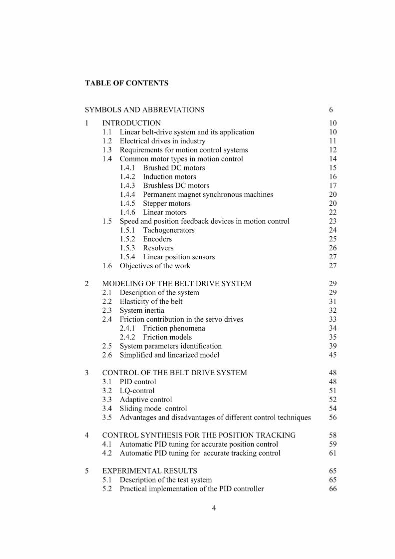
TABLE OF CONTENTS

SYMBOLS AND ABBREVIATIONS 6

1 INTRODUCTION 10 1.1 Linear belt-drive system and its application 10 1.2 Electrical drives in industry 11 1.3 Requirements for motion control systems 12 1.4 Common motor types in motion control 14

1.4.1 Brushed DC motors 15 1.4.2 Induction motors 16 1.4.3 Brushless DC motors 17 1.4.4 Permanent magnet synchronous machines 20 1.4.5 Stepper motors 20 1.4.6 Linear motors 22

1.5 Speed and position feedback devices in motion control 23 1.5.1 Tachogenerators 24 1.5.2 Encoders 25 1.5.3 Resolvers 26 1.5.4 Linear position sensors 27

1.6 Objectives of the work 27

2 MODELING OF THE BELT DRIVE SYSTEM 29 2.1 Description of the system 29 2.2 Elasticity of the belt 31 2.3 System inertia 32 2.4 Friction contribution in the servo drives 33

2.4.1 Friction phenomena 34 2.4.2 Friction models 35

2.5 System parameters identification 39 2.6 Simplified and linearized model 45

3 CONTROL OF THE BELT DRIVE SYSTEM 48

3.1 PID control 48 3.2 LQ-control 51 3.3 Adaptive control 52 3.4 Sliding mode control 54 3.5 Advantages and disadvantages of different control techniques 56

4 CONTROL SYNTHESIS FOR THE POSITION TRACKING 58

4.1 Automatic PID tuning for accurate position control 59 4.2 Automatic PID tuning for accurate tracking control 61

5 EXPERIMENTAL RESULTS 65

5.1 Description of the test system 65 5.2 Practical implementation of the PID controller 66

5

5.2.1 Selection of sample time 66 5.2.2 Discretization of the PID controller 67 5.2.3 Practical structure of the PID controller 69 5.2.4 Implementation in dSPACE 71

5.3 Comparison of the simulation and measurement results 72

6 CONCLUSIONS 77 REFERENCES 78 APPENDIX 81

6

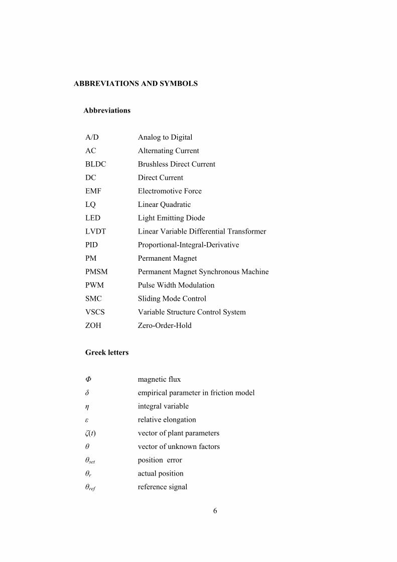
ABBREVIATIONS AND SYMBOLS

Abbreviations

A/D Analog to Digital

AC Alternating Current

BLDC Brushless Direct Current

DC Direct Current

EMF Electromotive Force

LQ Linear Quadratic

LED Light Emitting Diode

LVDT Linear Variable Differential Transformer

PID Proportional-Integral-Derivative

PM Permanent Magnet

PMSM Permanent Magnet Synchronous Machine

PWM Pulse Width Modulation

SMC Sliding Mode Control

VSCS Variable Structure Control System

ZOH Zero-Order-Hold

Greek letters

Φ magnetic flux

δ empirical parameter in friction model

η integral variable

ε relative elongation

ζ(t) vector of plant parameters

θ vector of unknown factors

θset position error

θr actual position

θref reference signal

7

ρ mass per unit volume

τ torque produced by motor

τf1, τf2 friction torques in the pulleys

τref torque reference

τmax maximum allowed value for torque reference

σ(x) sliding surface

φ angular position of motor shaft

ω rotation speed

ωset speed error

ωr actual rotor speed

ωref speed loop reference signal

Roman letters

A system matrix

B control matrix

C measurement matrix

D(s) transfer function of derivative term of PID controller

I(s) transfer function of integral term of PID controller

H width of the pulley

F friction force

Fapp applied force

Fc Coulomb friction

Fs static friction force

Fl external force applied longitudinally

Fv viscous friction force

G speed reducer ratio

J1, J2 inertia moments of driving and driven pulleys

Jcoupling inertia moment for coupling

Jencoder inertia moment for encoder

JG inertia moment for speed reducer

8

JM inertia moment for motor

K position feed back gain

K1, K2, K3 position dependent elasticity coefficients of the belt

Ke elasticity coefficient of the belt

Kd gain for proportional term of PID

Ki gain for integral term of PID

Kp gain for derivative term of PID

L transmission constant of the linear belt drive

Mc mass of the cart

P(s) transfer function of proportional term of PID controller

Q state weighting matrix

R radius of the pulley

Td derivative time

Ti integral time

Tt tracking constant

V volume

W(s) transfer function of PID controller

e electromotive force

es error signal in PID controller

e(t) error signal

f force produced in the motor

ff friction force which acts to the cart

g(t) command signal

h sample time

i armature current

iset current error

ir actual current

iref reference current

kv viscous friction coefficient

l1, l2, l stroke lengths

m mass

9

p1, p2, p3, p4 poles of the linearized simulation model

q1, q2 angular positions of the pulleys

r1 inner radius of the pulley

r2 outer radius of the pulley

r(t) reference signal

t time

u(x,t) control law

v sliding velocity

w belt stretch

x cart position

y(t) output signal

10

1 Introduction

1.1 Linear belt drive system and its application

Belt drives are widely used in different fields of human activity to transmit the mechanical

energy from the rotating shaft to the objects of the control. There are many examples of

belt drives implementation in our life such as cars, audio and video devices, computer

devices, etc. In industry such drives can be used for objects control positioning (for

instance, precise positioning of electronic chips on circuit plates) or transportation (for

example, conveyors).

Historically belt system has been used to transmit power at up to 98% efficiency between

rotational machine elements. Typical application for such system is a conveyor, the first

prototype of which has been used since 19th century. Moreover, already in 1913 Henry

Ford introduced the first conveyor belt-based assembly line in Ford Motor Company's

factory. Nowadays, belt drive systems are widely spread in automotive industry and in

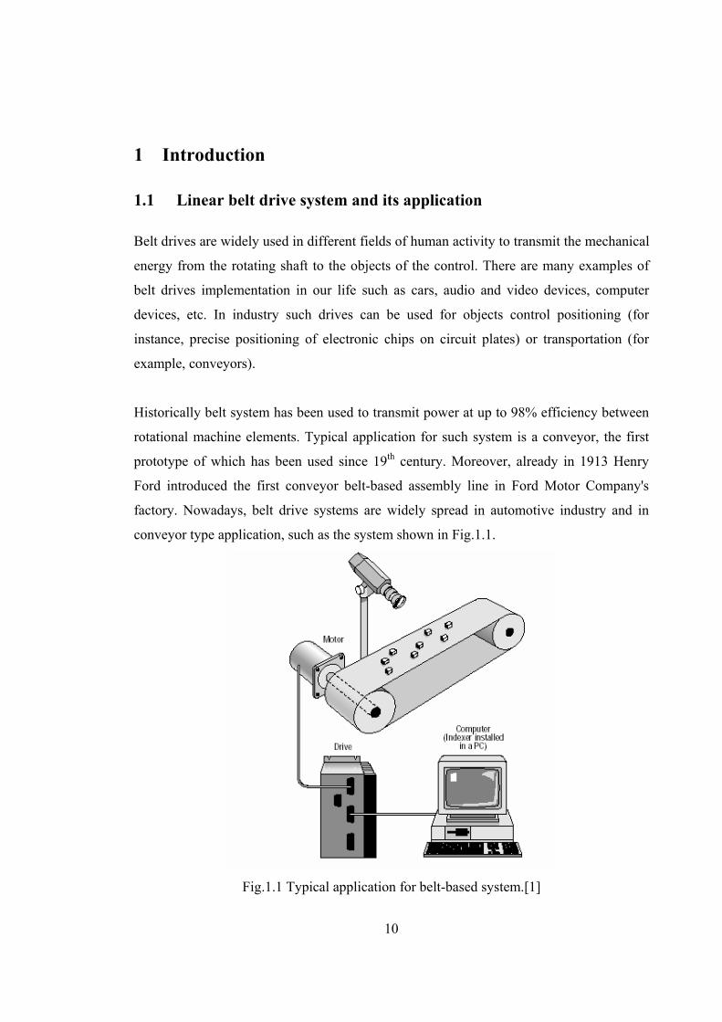
conveyor type application, such as the system shown in Fig.1.1.

Fig.1.1 Typical application for belt-based system.[1]

11

The system in Fig. 1.1 is applied for automated checking of small items for defect. It is

necessary to have a drive system to control the items to pass by the camera at constant

velocity and a computer control system for start and stop of the conveyor. Motion control

requirements for such system are accurate velocity control, linear motion and high

resolution.

Using of belt for high precision applications has become appropriate because of rapid

development of motor and drive technology as well as the implementation of timing belts

in belt-driven systems. Toothed or timing belts with correct tension exclude slippage and

increase the precision of motion. As a result, the use of belts in drives has caused a

number of advantages. Systems can provide high speed and acceleration, accurate and

repeatable motion, high efficiency, long stroke lengths and low cost. [2]

As a rule of thumb, belt drives use either the speed controlled drives if the rotation of

control object is needed or the servo drives if the position control is required.

1.2 Electrical drives in industry

The first electrical machine was invented in the first half of the 19th century. Since then

more than a century has passed. During this period, continuous improvements have been

developed for each application area of electrical machines and, as a result, electric motors

are nowadays a part of our everyday life. Many different motor types have been developed

in modern industry for hundreds of various purposes.

The object of attention in this work is servo drives. The term “servo” in context of motors

and drives means that they are used for the position control. [3] An electrical servo system

includes four main parts: a servomotor, a power converter, sensors and a load. Modern

closed-loop control systems allow the servo drives to achieve high dynamic performance

with high efficiency. The modern servo systems are characterized by the strong

requirements for the next important properties: [4]

• positioning accuracy

• speed accuracy

12

• torque stability

• overload capability

• dynamic performance

The typical applications for servo drives are robots, transfer lines, conveyors, lifts and

coordinate measuring systems. [5]

Analysis of publications [3]-[6] shows that servo drives are applied for example in such

areas of industry as:

• paper industry

• machine tools and metal working machinery

• packaging machinery

• woodworking

In spite of the wide spread occurrence of electrical motors, the precision requirements for

servo drives constantly increase. [7]

1.3 Requirements for motion control systems

Fig. 1.2 represents a standard scheme of servo drive system. The servo control is based on

a cascade principle, where the position reference for the position controller is fed by

higher-level controller. The position error θset, which is the difference between the

reference signal θref and the actual rotor position measured by a position sensor (such as

encoder as it is shown in Fig. 1.2) θr, go through the position controller that produces the

reference signal ωref for the speed control loop. The difference ωset between the speed loop

reference signal ωref and the actual rotor speed ωr, (which can be measured as a rate of

change of two successive positions), go to the speed controller, which produces the

reference signal iref for the current control loop. The error iset is the difference between the

reference current iref and the actual current is The current controller produces the output

signal, which is amplified by the power converter feeding voltage to the motor phases.

13

Fig. 1.2 Typical structure of servo control based on cascade principle. [8]

As it was mentioned above, a typical servo drive consists of four main parts. One of the

important belt drive design decisions that should be taken into account is the motor

selection. There are many available alternatives; each of them will have benefits and

disadvantages. Considering the whole servo system the motor determines the

characteristics of drive and it also determines the power converter and control

requirements. Many possibilities exist but only limited number will have enough broad

characteristics, which are required for the precise motion control. Summary is shown in

Table 1.1.

Table1.1 Requirements for machine-tool drive [6]

A high speed-to-torque ratio

Four-quadrant application

The ability to produce a torque at a standstill

A high power-to-weight ratio

High system reliability

14

The following motor types can satisfy the criteria given Table 1.1 and they are widely

used in servo systems:

• brushed DC motors

• brushless DC motors

• permanent magnet synchronous motors (PMSMs)

• induction motors

• stepper motors

• linear motors

The benefits and disadvantages of the each motor type are discussed in the next Section.

1.4 Common motor types in motion control

With invention of the motor the important question arisen is: how it can be controlled?

The first speed-controlled drive was introduced by Harry Ward Leonard and it required

three machines for scheme implementation. After the invention of transistor and rapid

development of electronics, new possibilities for accurate control of DC motor, such as

PWM technology, appeared. Brushless DC motors with permanent magnets were

introduced in early 1960s, but their power was limited due to not enough powerful PM

materials. Brushless DC motors for higher power application became available only after

the invention of PM materials with high energy density in the beginning of 1980s. Later

on, when the field-oriented control was introduced, it was possible to apply AC motors for

speed-controlled applications. First speed-controlled AC drives were induction motors but

in early 1990s the vector control was also developed for PMSMs. Also, with rapid

development of computer science became accessible control of stepper motors directly

from microcontrollers. All these motor types are available for wide range of motion

control applications. The most common of them are considered below in more detailed.

15

1.4.1 Brushed DC motors

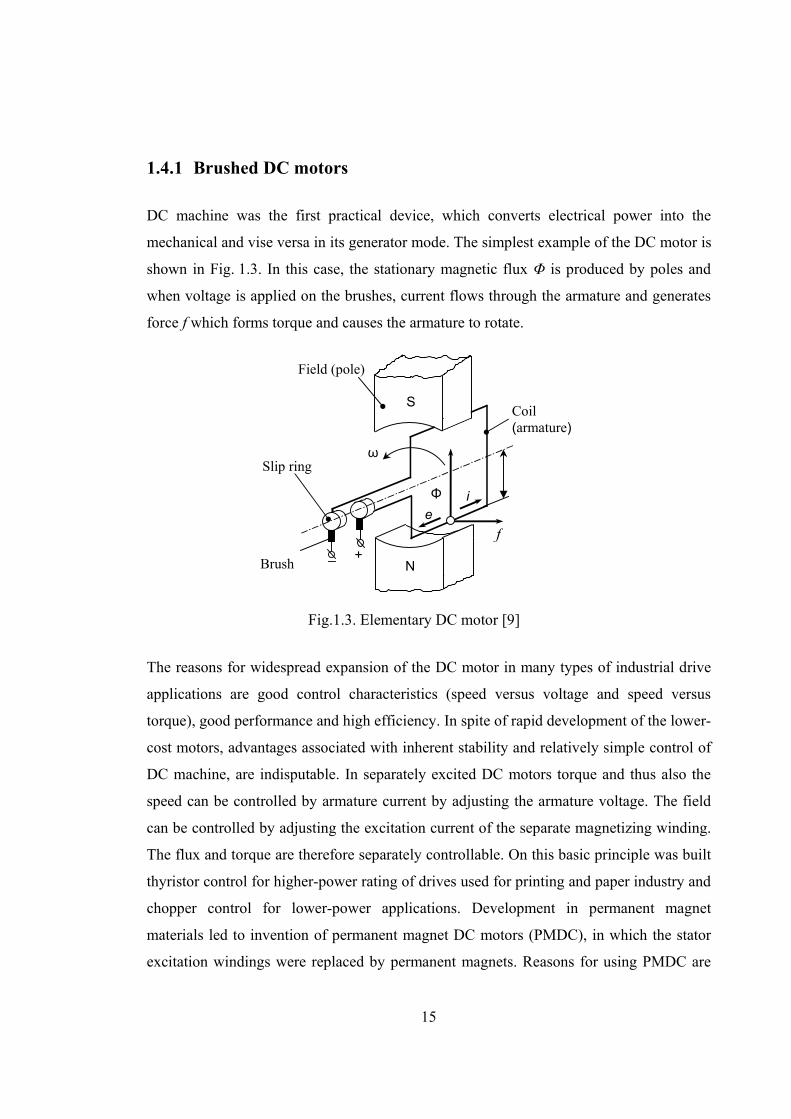
DC machine was the first practical device, which converts electrical power into the

mechanical and vise versa in its generator mode. The simplest example of the DC motor is

shown in Fig. 1.3. In this case, the stationary magnetic flux Φ is produced by poles and

when voltage is applied on the brushes, current flows through the armature and generates

force f which forms torque and causes the armature to rotate.

The reasons for widespread expansion of the DC motor in many types of industrial drive

applications are good control characteristics (speed versus voltage and speed versus

torque), good performance and high efficiency. In spite of rapid development of the lower-

cost motors, advantages associated with inherent stability and relatively simple control of

DC machine, are indisputable. In separately excited DC motors torque and thus also the

speed can be controlled by armature current by adjusting the armature voltage. The field

can be controlled by adjusting the excitation current of the separate magnetizing winding.

The flux and torque are therefore separately controllable. On this basic principle was built

thyristor control for higher-power rating of drives used for printing and paper industry and

chopper control for lower-power applications. Development in permanent magnet

materials led to invention of permanent magnet DC motors (PMDC), in which the stator

excitation windings were replaced by permanent magnets. Reasons for using PMDC are

S

N

ω

Brush

Slip ring

Coil (armature)

Field (pole)

f

iΦ

_ +

e

Fig.1.3. Elementary DC motor [9]

16

extremely linear speed-torque characteristics, small torque ripple at low speeds, absence of

copper losses in excitation windings and small rotor diameter.

The characteristics of the DC motors are not ideal for applications with strict requirements

for reliability, service interval and noises due to the mechanical and electrical limits set by

the motor commutator. In addition, the carbon brushes require regular service.

The other drawback of the DC motors is the fact that while the rotation speed increases,

the voltage between commutator segments also increases and in combination with high

armature current, a voltage breakdown between adjacent commutator segments will result

in motor brush fire or flashover. It should be avoided since it damages the commutator and

brush gear and reduces the life expectancy of the motor. Thus operational area of the

motor is bounded by different factors. Despite these disadvantages numerous applications

require drives based on brushed DC motors. In spite of the good control characteristics

enumerated drawbacks of DC motors are inconvenient for producing reliable high-

performance belt drives.

1.4.2 Induction motors

The AC squirrel-cage induction motors are the largest group of all electrical drives in the

industry. It has been estimated that they are used in 70-80% of all industrial drive

applications, especially in fixed-speed applications such as pump or fan drives. The

benefits of induction motor are undisputable: simple construction, low cost compared to

other motors, simple maintenance, high efficiency and satisfactory characteristics at the

high speeds. With appropriate power electronics converters induction motors are used in

wide power range from kW to MW levels.

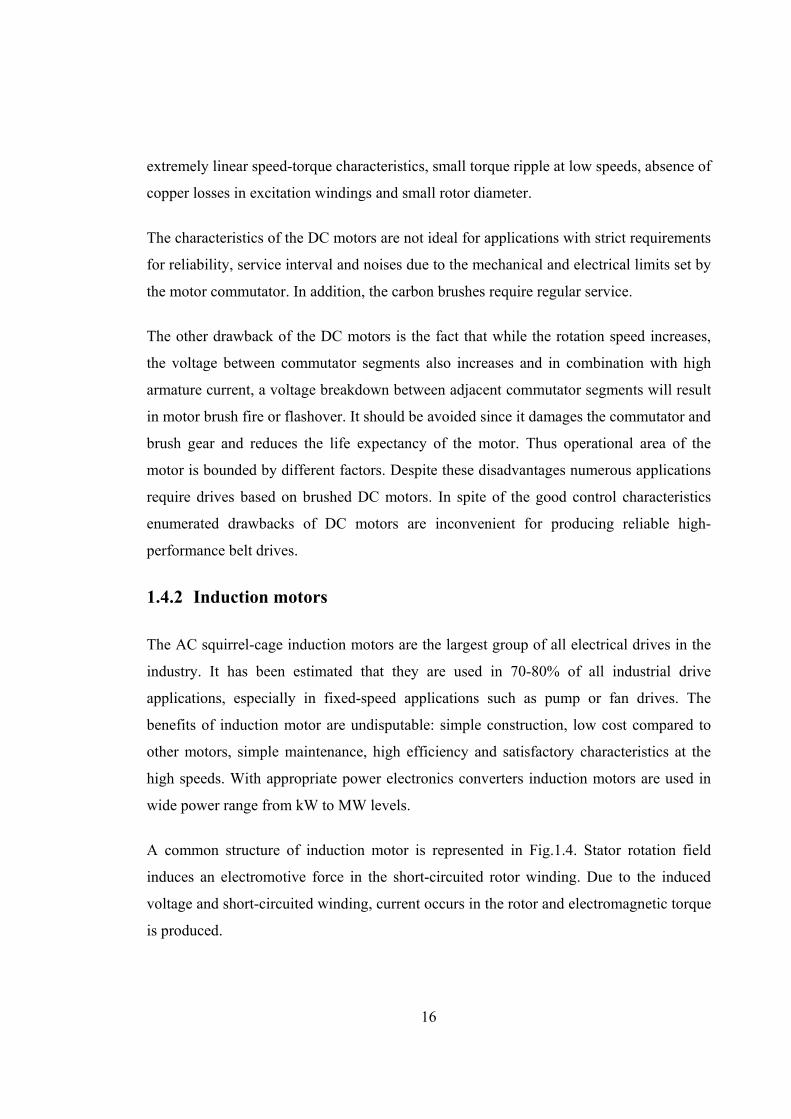
A common structure of induction motor is represented in Fig.1.4. Stator rotation field

induces an electromotive force in the short-circuited rotor winding. Due to the induced

voltage and short-circuited winding, current occurs in the rotor and electromagnetic torque

is produced.

17

Induction motor was invented in the end of 19th century. Its theory is well-known and

power electronic converter technology provides appropriate variable-voltage/current,

variable-frequency supply for efficient and stable variable-speed control. Thus, it is

possible to obtain a dynamic performance in all respects better than which could be

obtained with a phase-controlled DC drive combination. The significant characteristic of

the induction motor is a slip caused by the rotor lagging the rotating stator magnetic field.

Rotor copper losses are directly proportional to the slip. For example, the rotor copper

losses in 4 kW motor are approximately 4.7% of the nominal power if the efficiency of

85% is supposed. [10] The slip has also impact when a high dynamic performance is

needed, since it derates the transient response of the motor.

The main disadvantage of the induction motor for the servo control systems is the non-

linear speed versus torque and speed versus control voltage characteristics. Therefore such

motors are inconvenient for the implementation of the belt-drives.

1.4.3 Brushless DC motors

An impetus to the recent development of brushless DC motors was given by computer-

peripheral and aerospace industries, where high performance coupled with reliability and

low maintenance are essential. [3] Typically, the brushless DC motor has a three-phase

stator, and the rotor has surface-mounted magnets that create rectangular air gap flux

distribution. The motor is driven by rectangular or trapezoidal voltage pulses paired with

the given rotor position. In order to generate the maximum torque, the angle between the

Fig.1.4. Common structure of induction machine.

18

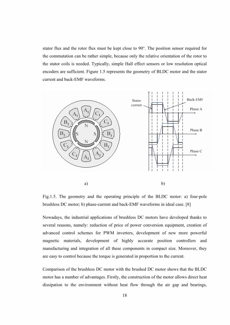
stator flux and the rotor flux must be kept close to 90°. The position sensor required for

the commutation can be rather simple, because only the relative orientation of the rotor to

the stator coils is needed. Typically, simple Hall effect sensors or low resolution optical

encoders are sufficient. Figure 1.5 represents the geometry of BLDC motor and the stator

current and back-EMF waveforms.

a) b)

Fig.1.5. The geometry and the operating principle of the BLDC motor: a) four-pole

brushless DC motor; b) phase-current and back-EMF waveforms in ideal case. [8]

Nowadays, the industrial applications of brushless DC motors have developed thanks to

several reasons, namely: reduction of price of power conversion equipment, creation of

advanced control schemes for PWM inverters, development of new more powerful

magnetic materials, development of highly accurate position controllers and

manufacturing and integration of all these components in compact size. Moreover, they

are easy to control because the torque is generated in proportion to the current.

Comparison of the brushless DC motor with the brushed DC motor shows that the BLDC

motor has a number of advantages. Firstly, the construction of the motor allows direct heat

dissipation to the environment without heat flow through the air gap and bearings,

19

therefore additional cooling system is not usually required. Secondly, brushless DC

motors provide more accurate overload protection, because the temperature of the hottest

part can be detected directly [5]. In addition, some advantages are connected with absence

of mechanical commutator:

• There is no sparking; that is the motor can be used in hazardous environments.

• Maintenance costs are reduced; brushless DC motors do not require regular

service of the brush gear.

• The speed-torque limits caused by commutator are eliminated.

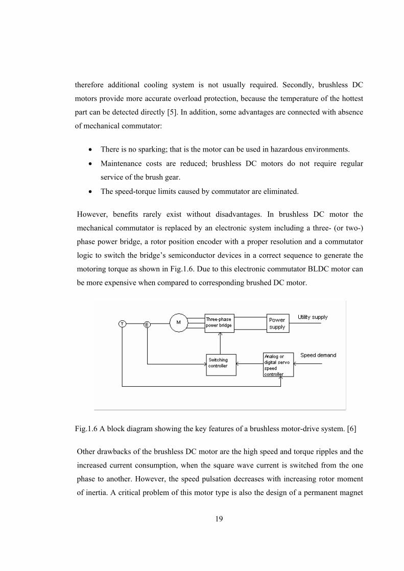
However, benefits rarely exist without disadvantages. In brushless DC motor the

mechanical commutator is replaced by an electronic system including a three- (or two-)

phase power bridge, a rotor position encoder with a proper resolution and a commutator

logic to switch the bridge’s semiconductor devices in a correct sequence to generate the

motoring torque as shown in Fig.1.6. Due to this electronic commutator BLDC motor can

be more expensive when compared to corresponding brushed DC motor.

Fig.1.6 A block diagram showing the key features of a brushless motor-drive system. [6]

Other drawbacks of the brushless DC motor are the high speed and torque ripples and the

increased current consumption, when the square wave current is switched from the one

phase to another. However, the speed pulsation decreases with increasing rotor moment

of inertia. A critical problem of this motor type is also the design of a permanent magnet

20

rotor, because there is the possibility of the failure of magnet-rotor junction at high

rotational speed and accelerations. As a result, the brushless DC motors are widely used

for power outputs up to 20kW [6]. Above this power level vector-controlled induction

motors are dominating. Therefore it can be concluded that the brushless DC motors can

be used in low-cost belt-drives.

1.4.4 Permanent magnet synchronous machines (PMSM)

Permanent magnet synchronous machines emerged into servo drives since the second part

of the 20th century and, nowadays, this motor type is widely spread in industry, especially

in windmill generators and propulsion motors. [8] Main disadvantages of early permanent

magnet motors were the risk of demagnetization of magnets by high stator currents during

starting and the restricted maximum allowable temperature. The development of high-

quality permanent magnet materials during the 1970s overcame these problems. PMSM’s

mechanical and electrical characteristics, especially the inductances, are highly dependent

on the rotor structure. PMSMs can be realized either with embedded or surface magnets

on the rotor. As the relative permeability of modern magnet materials is close to unity, the

effective air gap becomes large with a surface magnet construction. As a result, the direct

axis inductance of the machine remains low, which improves the overloading capability of

the motor but at the cost of the reduced field weakening range. Another advantage of such

a motor configuration is low inertia.

Permanent magnet synchronous motors are very good alternatives for belt drives due to

very good control characteristics and the absence of the mechanical commutator. The

drawback of PMSM is their relatively higher costs compared to the other types of motors.

1.4.5 Stepper motors

Stepper motors have become popular because they can be controlled directly by

computers, microprocessors or programmable microcontrollers, thanks to their ability to

rotate output shaft in angular steps corresponding to discrete signals fed into a controller.

The signals are converted into current pulses switched to the motor coils in fixed order

21

and, thus, the motor works as an incremental actuator, which transforms digital pulses into

analog output in form of shaft rotation. The rotational speed depends on the pulse rate and

the incremental step angle, where the angle of rotation is dependent on the number of

pulses received from the controller and the incremental step angle. These features make

stepper motors appropriate to the open-loop position and speed control. Typical

applications include disc head drives, small machine tool slides and printer head drives,

where the motor might drive the head directly or via a belt. The following characteristics

make the stepper motor suitable for servo drive applications:

• Stepper motors can work with a basic accuracy of ± 1 step in open-loop system.

The inherent accuracy of the motor removes the requirements for the position and

speed transducers and hence reduces the cost of the overall system.

• Stepper motors can generate high output torques at low angular velocities.

• Connection circuitry of the stepper motor is digital simplifying the interface to the

programmable controller or control computer.

• Mechanical construction of the stepper motor is simple and robust.

However, an important point, which should be mentioned, is the phenomenon of

resonance suffered by all stepper motors to some degree. As was mentioned above,

stepper motor is controlled by pulses from the digital circuit. The step pulses are usually

generated by an oscillator circuit controlled by an analog voltage, a digital controller or a

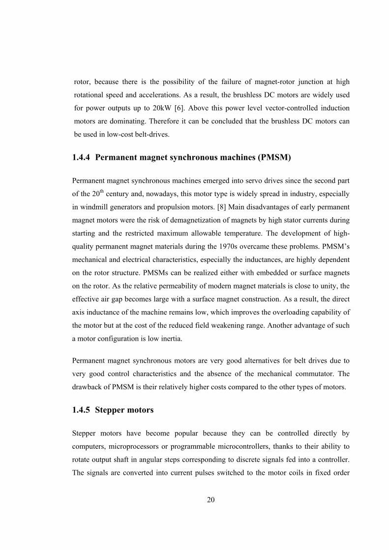
microprocessor. A response to the sequence of five equally spaced step pulses in time is

shown in Fig. 1.7.

22

Fig.1.7 Typical step-response to low-frequency order of step pulses. [3]

Three main quantities can be noted from Fig.1.7. Firstly, the total shaft angle after five

steps, is generated by only the number of pulses, in such a way that the average speed of

the shaft depends on the step pulse frequency. Hence, the higher frequency the less time is

required for execution of the five steps. Secondly, a single step operation is not ideal, and

therefore single-step times vary with motor size, step angle and the nature of load. Thirdly,

it is necessary to know the initial rotor position for the calculation of the absolute position

after a step sequence, because the stepper motor is an incremental device. Normally, the

step counter should be “zeroed” when the motor shaft is at its initial position.

As a consequence the stepper motor can be applied in very particular applications due to

its specific characteristics.

1.4.6 Linear motors

Nowadays linear applications are more demanding than ever before. There are many

brushless linear motors available for the motion control with large stroke length, high

speed and accuracy, load capacity and stiffness at the moment. The linear motor concept is

not new. Early machines had limitations in high speed operation due to commutation bar

23

and brushes. Brushless servo motor technology and implementation electronics to drive

them allow avoiding the above limitations. Commutation is manufactured electronically

by Hall-effect sensors and therefore commutation is not limiting factor. Thus, brushless

linear motors have a sum of advantages:

• High speed operation. The maximum of linear motor speed is bounded only bus

voltage and speed of control electronics. Typical speed of linear motor is 3 meters

per second with 1 micron resolution.[11]

• High precision. The accuracy, resolution and repeatability of motor depend on

controlled feedback device. Wide range of linear feedback devices allow to

appropriate device limiting only control system bandwidth.

• Fast response. The response rate of a linear motor driven device can be over 100

that of a mechanical transmission. [11]

• Zero backlash. No backlash due to absence of mechanical transmission

components.

• Maintenance free operation. There is no wear due to absence of contacting parts in

modern linear motors.

Side by side with all benefits, list of drawbacks such as high cost, sizing, heating exists.

The usage of linear motors can prevent the using of non-desirable belts in the systems and

therefore can increase the accuracy of the system. But such decision can have the big cost

and sizing problems.

1.5 Speed and position feedback devices in motion control

The precise control of speed, position or acceleration requires appropriate measuring

systems for detection controlled variable. In this case measured quantities are rapidly

changing therefore necessary to consider dynamic relationship between input and output

of measurement system. In contrast, measured variable can be changed slowly in some

kind of systems, hence the static performance should be considered. Before considering

24

the various forms of sensor, it is necessary to mention significant characteristics such as

resolution and accuracy.

The resolution of feedback device can be described as a number of measuring step per

revolution of the motor shaft, for instance, resolution for incremental encoder is number of

pulses per revolution. For analog feedback devices such as resolvers, resolution refers to

associated resolver-to-digital converters.

The accuracy of sensor can be described as position deviation within one measuring step.

In encoder accuracy directly depends on the eccentricity of the graduation to the bearing,

the elasticity of the encoder shaft and its coupling to the motor shaft, the graduation and

the electronic signal processing. For analog feedback devices the accuracy is influenced

by the winding distribution, eccentricity of the air gap, uniformity of the air-gap flux and

elasticity of the resolver shaft and its coupling to the motor shaft.

1.5.1 Tachogenerators

The DC tachogenerator is electromagnetic transducer that converts mechanical rotation

into DC output voltage commonly used as speed feedback device. The output voltage is

directly proportional to the rotational speed. The basic fundamentals of tachogenerators

are the same as DC motor, besides, significant features of its operation are following:

• Linearity of the output; that is output voltage proportional to the shaft speed with

defined linearity.

• Smooth output; the output voltage should be free from ripple in range of frequency

where drive is operating

• Independence output voltage of temperature; the output voltage for given speed

should be constant with changing temperature.

Nevertheless, output characteristics of the tachogenerators are not ideal. The peak-to-peak

value of output ripple-voltage component is reached 5-6%, with using special equipment

is around 2-3%. [6] The temperature influence on characteristics is existed and quality of

this parameter is closely related to the design principle and materials used in manufacture

25

of the tachogenerators. Also linearity of output voltage can be affected by hysteresis losses

in the armature core, output current drain, armature reaction and saturation effect

particularly in very-high speed applications. In that way, application of tachogenerators

can be quite reasonable in motion control systems if speed transducer is required.

1.5.2 Encoders

While the velocity can be determined from position measurements, encoders are able to

provide a separate output which is proportional to the velocity. Encoders are widely used

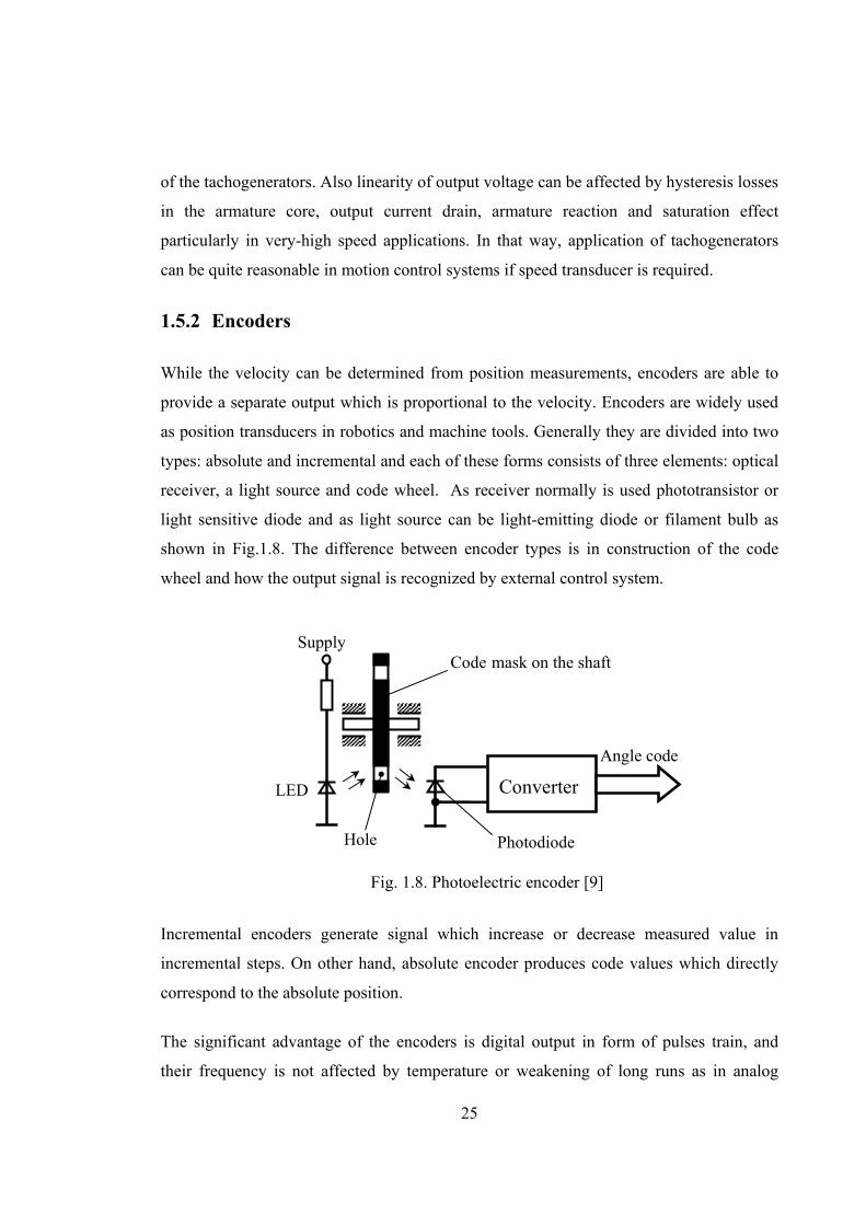
as position transducers in robotics and machine tools. Generally they are divided into two

types: absolute and incremental and each of these forms consists of three elements: optical

receiver, a light source and code wheel. As receiver normally is used phototransistor or

light sensitive diode and as light source can be light-emitting diode or filament bulb as

shown in Fig.1.8. The difference between encoder types is in construction of the code

wheel and how the output signal is recognized by external control system.

Incremental encoders generate signal which increase or decrease measured value in

incremental steps. On other hand, absolute encoder produces code values which directly

correspond to the absolute position.

The significant advantage of the encoders is digital output in form of pulses train, and

their frequency is not affected by temperature or weakening of long runs as in analog

Code mask on the shaft

Angle code

Supply

Hole

ConverterLED

Photodiode

Fig. 1.8. Photoelectric encoder [9]

26

signal generator or resolver, therefore it is more reasonable using encoders in digital

control systems.

1.5.3 Resolvers

The resolver is related to the synchro group. Synchro is meant the group of angular

position sensing devices which can provide a rotational torque for light loads or signal

which was caused by this rotational torque. A resolver is modified form of synchro which

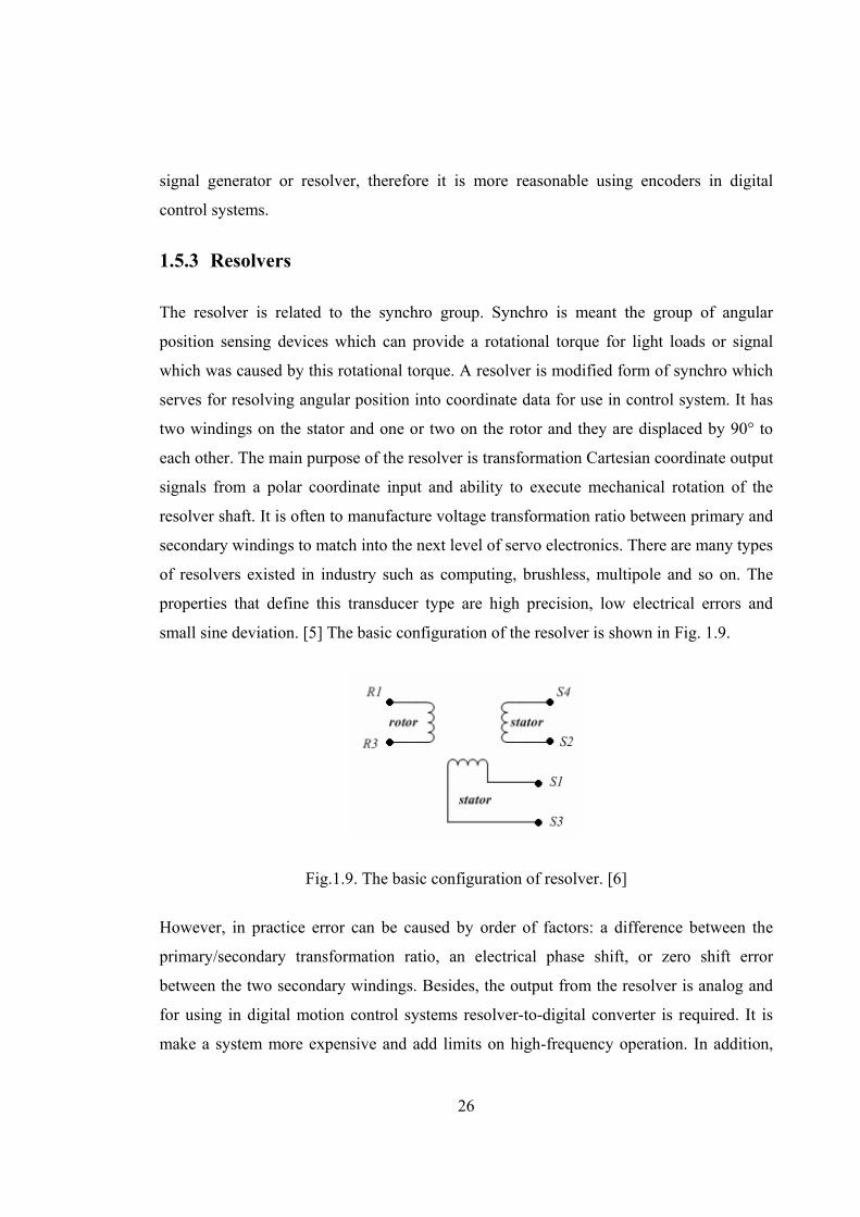
serves for resolving angular position into coordinate data for use in control system. It has

two windings on the stator and one or two on the rotor and they are displaced by 90° to

each other. The main purpose of the resolver is transformation Cartesian coordinate output

signals from a polar coordinate input and ability to execute mechanical rotation of the

resolver shaft. It is often to manufacture voltage transformation ratio between primary and

secondary windings to match into the next level of servo electronics. There are many types

of resolvers existed in industry such as computing, brushless, multipole and so on. The

properties that define this transducer type are high precision, low electrical errors and

small sine deviation. [5] The basic configuration of the resolver is shown in Fig. 1.9.

Fig.1.9. The basic configuration of resolver. [6]

However, in practice error can be caused by order of factors: a difference between the

primary/secondary transformation ratio, an electrical phase shift, or zero shift error

between the two secondary windings. Besides, the output from the resolver is analog and

for using in digital motion control systems resolver-to-digital converter is required. It is

make a system more expensive and add limits on high-frequency operation. In addition,

27

resolvers are very sensitive devices but limited by input signal range and has not compact

dimensions, therefore using its in belt-drive systems is not reasonable.

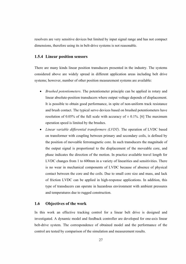
1.5.4 Linear position sensors

There are many kinds linear position transducers presented in the industry. The systems

considered above are widely spread in different application areas including belt drive

systems; however, number of other position measurement systems are available:

• Brushed potentiometers. The potentiometer principle can be applied in rotary and

linear absolute-position transducers where output voltage depends of displacement.

It is possible to obtain good performance, in spite of non-uniform track resistance

and brush contact. The typical servo devices based on brushed potentiometers have

resolution of 0.05% of the full scale with accuracy of ± 0.1%. [6] The maximum

operation speed is limited by the brushes.

• Linear variable differential transformers (LVDT). The operation of LVDC based

on transformer with coupling between primary and secondary coils, is defined by

the position of moveable ferromagnetic core. In such transducers the magnitude of

the output signal is proportional to the displacement of the moveable core, and

phase indicates the direction of the motion. In practice available travel length for

LVDC changes from 1 to 600mm in a variety of linearities and sensitivities. There

is no wear in mechanical components of LVDC because of absence of physical

contact between the core and the coils. Due to small core size and mass, and lack

of friction LVDC can be applied in high-response applications. In addition, this

type of transducers can operate in hazardous environment with ambient pressures

and temperatures due to rugged construction.

1.6 Objectives of the work

In this work an effective tracking control for a linear belt drive is designed and

investigated. A dynamic model and feedback controller are developed for one-axis linear

belt-drive system. The correspondence of obtained model and the performance of the

control are tested by comparison of the simulation and measurement results.

28

For the basis of linear belt drives studies the main problems of dynamic modeling and

tracking control design should be formulated. The first group of challenges related to the

friction and the non-linear belt flexibility with respect to load position should be

considered. In addition, the selection and implementation of the control strategy should

base on the obtained dynamic model. So, the computer model of the system must

correspond to real test drive.

Decision of above mentioned modeling problems should be done with separate

investigation of different aspects of the belt drive model and their influence to the system

dynamics. Also decision about effective control strategy should be done with literature

based survey of control methods for linear belt drives. The effectiveness of chosen control

method should be demonstrated practically on experimental test setup. The results of the

work are shown by comparison of simulation and measurements curves.

29

2 Modeling of the belt drive system 2.1 Description of the system

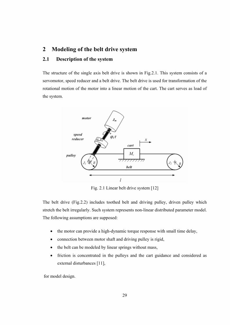
The structure of the single axis belt drive is shown in Fig.2.1. This system consists of a

servomotor, speed reducer and a belt drive. The belt drive is used for transformation of the

rotational motion of the motor into a linear motion of the cart. The cart serves as load of

the system.

Fig. 2.1 Linear belt drive system [12]

The belt drive (Fig.2.2) includes toothed belt and driving pulley, driven pulley which

stretch the belt irregularly. Such system represents non-linear distributed parameter model.

The following assumptions are supposed:

• the motor can provide a high-dynamic torque response with small time delay,

• connection between motor shaft and driving pulley is rigid,

• the belt can be modeled by linear springs without mass,

• friction is concentrated in the pulleys and the cart guidance and considered as

external disturbances [11],

for model design.

30

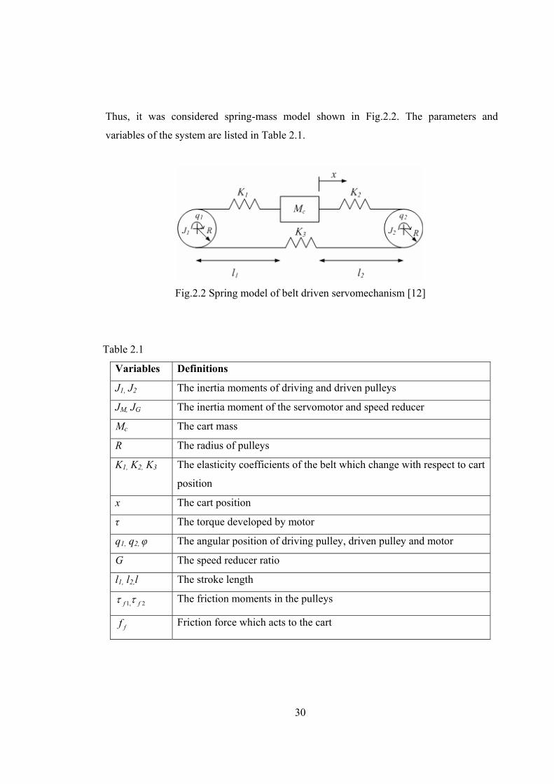
Thus, it was considered spring-mass model shown in Fig.2.2. The parameters and

variables of the system are listed in Table 2.1.

Fig.2.2 Spring model of belt driven servomechanism [12]

Table 2.1

Variables Definitions

J1, J2 The inertia moments of driving and driven pulleys

JM, JG The inertia moment of the servomotor and speed reducer

Mc The cart mass

R The radius of pulleys

K1, K2, K3 The elasticity coefficients of the belt which change with respect to cart

position

x The cart position

τ The torque developed by motor

q1, q2, φ The angular position of driving pulley, driven pulley and motor

G The speed reducer ratio

l1, l2,l The stroke length

2,1 ff ττ The friction moments in the pulleys

ff Friction force which acts to the cart

31

Mathematical model for belt drive system, which is shown in Fig.2.2, is represented as

equation system [11]

),()()(

)]())(([

)]())(([))((

2211

12312222

12311112

1

RqxKxRqxKfxM

RqRqKxRqxKrqJ

RqRqKxRqxKrGqJJGJ

fc

f

fmG

−⋅−−⋅=+

−⋅−−⋅=+

−⋅−−⋅−⋅=+⋅+⋅+

&&

&&

&&

τ

ττ

(2.1)

where ))(( 21 mG JJGJ +⋅+ is the total moment of inertia, referred to the drive pulley,

τ⋅G - torque, referred to the drive.

Consequently, the model of the given belt drive system can be implemented by realization

system equations (2.1) in Simulink model. In addition, it is necessary to define parameters

of the model additionally such as position dependent elasticity coefficients, inertia system

and friction model satisfied to the dynamic performance of the real belt drive system.

2.2 Flexibility of the belt

As was assumed, the belt has elasticity properties; therefore it is possible to change the

length through the application external forces, caused by motor torque and cart mass. This

quantity can be described by generalized Hooke’s law in terms of the consepts of stress

and strain. Stress is a quantity that is proportional to the force causing a deformation;

strain is the measure of the degree of the deformation. In that way, according to

generalized Hooke’s law the tensile stress σ is linearly proportional to the strain ε by a

constant factor called elastic modulus E.

εσ E= (2.2)

In term of belt drive systems, position dependent coefficients K1, K2 can be found as

elastic modulus; that is

,)( xl

FK

i

li −=ε

(2.3)

where lF is the external force applied longitudinally,

32

ill∆

=ε is the ratio of the change in length l∆ to the original length il ,

)( xli − is addition stretch component caused by cart position.

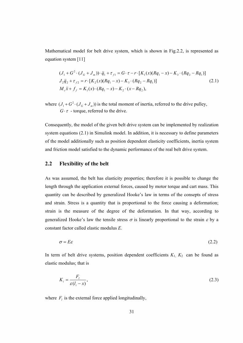
As result, belt flexibility can be implemented in Simulink (Fig.2.3) by including the Fcn

block, which realizes position dependent Ki(x) using Eq. (2.3), multiplied by the

displacement in accordance with Eq. (2.2).

Fig.2.3 Implementation of the generalized form of Hooke’s law in MATLAB®Simulink.

2.3 System inertia

Now should be considered system inertia for effective modeling of the whole belt-drive

system. It is necessary to take into account all part of the system. Thus, the inertia of belt

drive system JDS must include the contribution from all rotational elements, including the

idlers, reducer, coupling, which connected motor shaft with the driving pulley, encoder

and motor; that is

encoderGcouplingMDS JJJJJJJ +++++= 21 , (2.4)

where MG JJJJ ,,, 21 are the moments of inertia defined in Table 2.1

couplingJ is the moment of inertia for coupling which connects the motor shaft to the

driving pulley,

encoderJ is moment of inertia for incremental encoder.

33

The parameters of components can be obtained from the appropriate technical data sheets.

Moments of inertia for driving and driven pulleys are supposed equal and can be

calculated from integral equation [13]

∫= dVrJ 21 ρ , (2.5)

where ρ is mass per unit volume and can be defined as

dVdm

Vm=

∆∆

= limρ (2.6)

dVdm ρ= (2.7)

Thus, moment of inertia of the pulley is described by expression

2)(

24

14

2321

2

1

rrLdrrLdmrJ

r

r

−=== ∫∫πρ

πρ , (2.8)

where 1r and 2r are the inner and outer radius of the pulley, respectively and L is the width

of the pulley.

2.4 Friction contribution in the servo drives

In servo systems friction has an influence on the system dynamics in all modes of

operation. Friction serves to perform damping action at all frequencies, especially it has

impact on the bandwidth of control. At upper limits of performance friction affects to

design the time optimal control and define the limits of speed and power. Friction

contributes to the system dynamic during its performance and in some cases friction force

can dominate the forces of the motion, thus friction should be modeled for precise

compensation.

On the low bounds of system performance such as a minimum achievable displacement

and a minimum possible velocity friction affects also. These bounds increase from a

34

periodic process of sticking and sliding, which is generated by the non-linear, low velocity

friction.

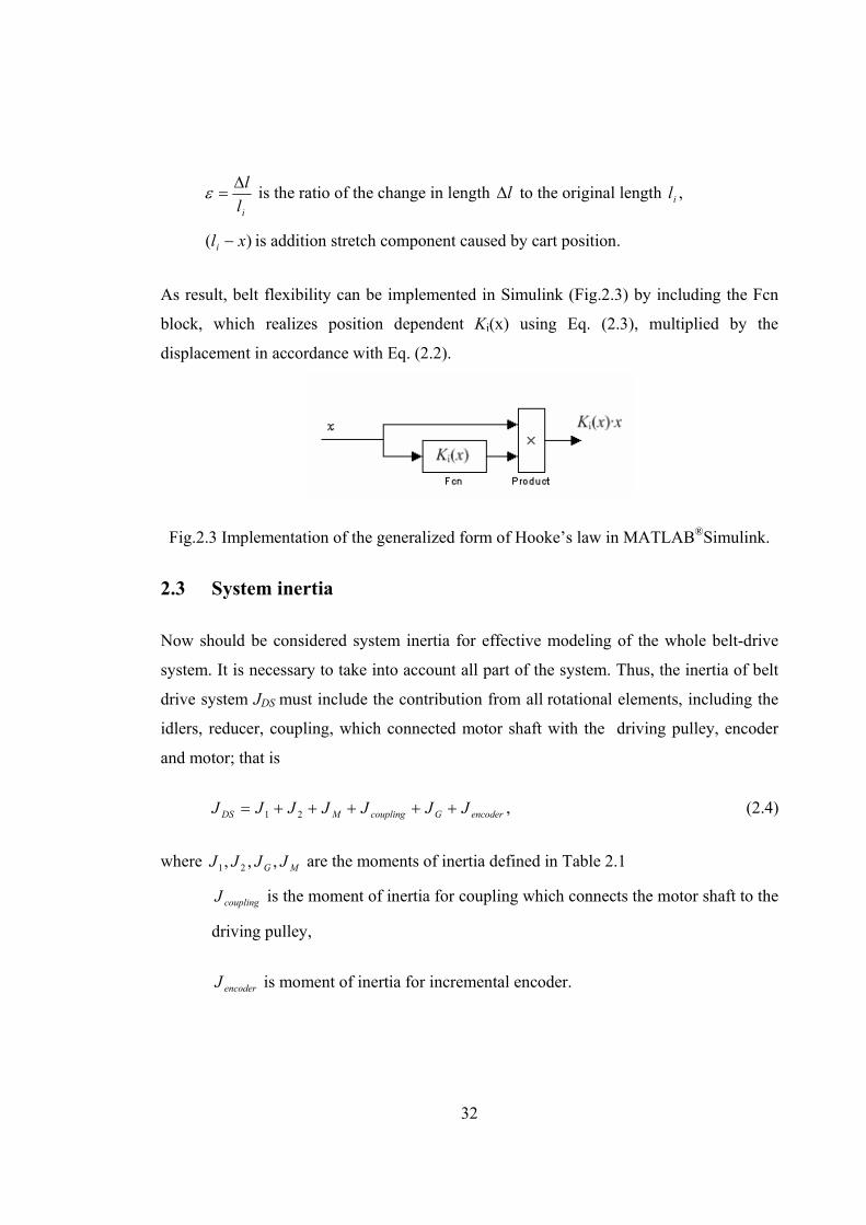
2.4.1 Friction phenomena

For understanding friction phenomena it is necessary to consider the topography of the

contacting surfaces. In fact, the interacting surfaces can be investigated by considering

smaller contacts, because each surface even regarded as smooth, is microscopically rough.

Contact consists of only separate points as shown in Fig.2.4a. Deformation of contact

increases with load increasing, thus the junction area between part A and part B grows.

Fig. 2.4 a) Part-to-part contact at asperities; b) Stribeck curve which shows friction versus

velocity at low velocity area. [14]

Typically, oil or grease is used to lubricate the contact. In the absence of lubricants an

oxide film will be formed on the steel surface or on the other materials as a boundary

layer. When the lubricant is present, the additives of the oil bulk react with the surface to

form the boundary layer. Friction is proportional to the shear strength of asperity

junctions, which are deformed by the total load. When the boundary layer has low shear

strength, the friction will be low respectively.

There are four velocity dependent regimes in the lubricated contacts as shown in Fig.2.4b,

which represent the Stribeck curve.

35

Regime 1: Static friction

No motion without sliding. Friction is caused by plastic deformation of asperity junctions

and boundary films.

Regime 2: Boundary lubrication

Boundary lubricants reduce the static friction. Friction in boundary lubrication is higher

than friction in regimes three and four, because of there is solid-to-solid contact.

Regime 3: Partial fluid lubrication

In this regime friction is produced partly lubricant viscosity and partly asperity junctions,

when lubrication layer is thinker than asperity height.

Regime 4: Full fluid lubrication

Solid-to-solid contact is totally eliminated. Friction in this regime has dependence of

hydrodynamic of the lubricant.

The transfer from one regime to another is very complicated and can not be described only

as a function of the velocity. More complex consideration of friction phenomena have

been represented in Armstrong-Helouvry [14].

2.4.2 Friction models

As mentioned above, friction is very complicated phenomenon. In given circumstances,

some effects can dominate over others and some of them can not be detectable with

sensible technology. Nevertheless, all described phenomena are present all the time. The

use of more complex friction model can exactly describe friction features and extend the

applicability of analytical results.

In the following, reviews of commonly used friction models are given.

36

• Static friction: At zero velocity, static friction opposes to all motion until the

applied force magnitude Fapp is less than the maximum stiction force Fs

where v is sliding velocity.

• Coulomb friction: The friction force always opposes the relative motion. It is

independent of the contact area and the relative velocity magnitude. In addition,

Coulomb friction is proportional to the normal force and can be described by

)sgn(vFF c= (2.10)

where Fc is Coulomb friction.

• Viscous friction: Viscous friction is proportional to the velocity and produced by

the viscosity of lubricants. Mathematically viscous friction can be expressed as

vkF v= (2.11)

where kv is the viscous friction coefficient.

• Exponential model : A very common form of the combined friction model

comprising of Coulomb and viscous frictions and also the Stribeck effect is

xFxxFFxFxF vscsc &&&&& +−−+= ))/(exp()()sgn()( δ

(2.12)

where sx& and δ are empirical parameters. By choosing different parameters,

different frictions can be implemented. Range of δ can be large [14]. The

exponential model (2.12) gives a Gaussian model with δ=2, which is nearly

if v=0 and |Fapp|< Fs (2.9)

if v=0 and |Fapp|≥ Fs ,

=)Fsgn(F

FF

apps

app

37

equivalent to Lorentzian model. On the other side, δ=1 gives Tustin’s model

which given by

xFxxFFxFxF vscsc &&&&& +−−+= ))/(exp()()sgn()( . (2.13)

It is one of the best models to describe the friction force near zero speeds. Tustin

was the first in feedback control who made a model with negative viscous friction

(Stribeck effect). He predicts the oscillations at low speed. Experimental works

shows that this model can approximate the real friction with high precision. [16]

By variation parameters of exponential model can be obtained models for specific

lubricants and conditions.

The most widely used frictions models in practical servo control systems are based

on different combinations of Eqs.(2.9-2.11) as represented in Fig. 2.5.

Fig.2.5. a) Coulomb friction, b) Coulomb friction plus viscous friction, c) Static friction

plus Coulomb and viscous friction, d) Stribeck curve shows effect of decreasing friction

with increasing velocity. [15]

The Tustin’s friction model was chosen for implementation in the belt-drive system. It

satisfactory describes the friction at low speeds and may help to model the possible

oscillations in the beginning of the movement. The Simulink block diagram of Tustin’s

friction model is shown in Fig.2.6.

38

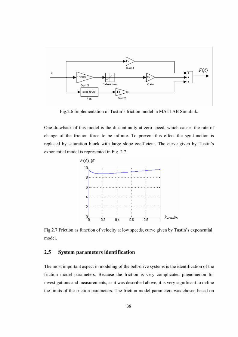
Fig.2.6 Implementation of Tustin’s friction model in MATLAB Simulink.

One drawback of this model is the discontinuity at zero speed, which causes the rate of

change of the friction force to be infinite. To prevent this effect the sgn-function is

replaced by saturation block with large slope coefficient. The curve given by Tustin’s

exponential model is represented in Fig. 2.7.

Fig.2.7 Friction as function of velocity at low speeds, curve given by Tustin’s exponential

model.

2.5 System parameters identification

The most important aspect in modeling of the belt-drive systems is the identification of the

friction model parameters. Because the friction is very complicated phenomenon for

investigations and measurements, as it was described above, it is very significant to define

the limits of the friction parameters. The friction model parameters was chosen based on

39

the measured transients processes of the angular position of the pulley and the cart

position with the fixed pulse of torque reference. A special attention was paid to the

accurate prediction of the shape of the velocity response obtained from the incremental

encoder. An estimate of the stiction was measured by experiment series, the results of

which are presented in Appendix 1.

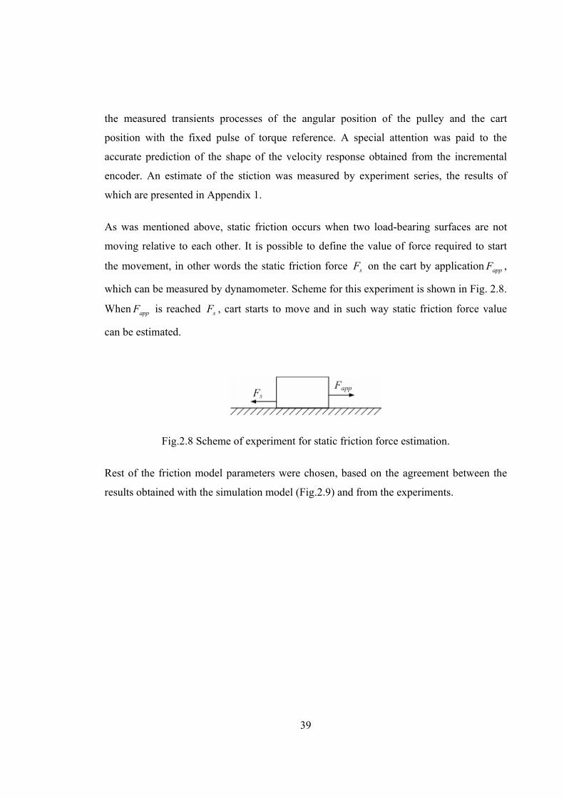
As was mentioned above, static friction occurs when two load-bearing surfaces are not

moving relative to each other. It is possible to define the value of force required to start

the movement, in other words the static friction force sF on the cart by application appF ,

which can be measured by dynamometer. Scheme for this experiment is shown in Fig. 2.8.

When appF is reached sF , cart starts to move and in such way static friction force value

can be estimated.

Fig.2.8 Scheme of experiment for static friction force estimation.

Rest of the friction model parameters were chosen, based on the agreement between the

results obtained with the simulation model (Fig.2.9) and from the experiments.

40

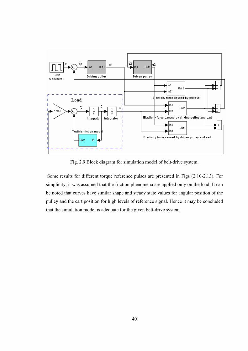
Fig. 2.9 Block diagram for simulation model of belt-drive system.

Some results for different torque reference pulses are presented in Figs (2.10-2.13). For

simplicity, it was assumed that the friction phenomena are applied only on the load. It can

be noted that curves have similar shape and steady state values for angular position of the

pulley and the cart position for high levels of reference signal. Hence it may be concluded

that the simulation model is adequate for the given belt-drive system.

41

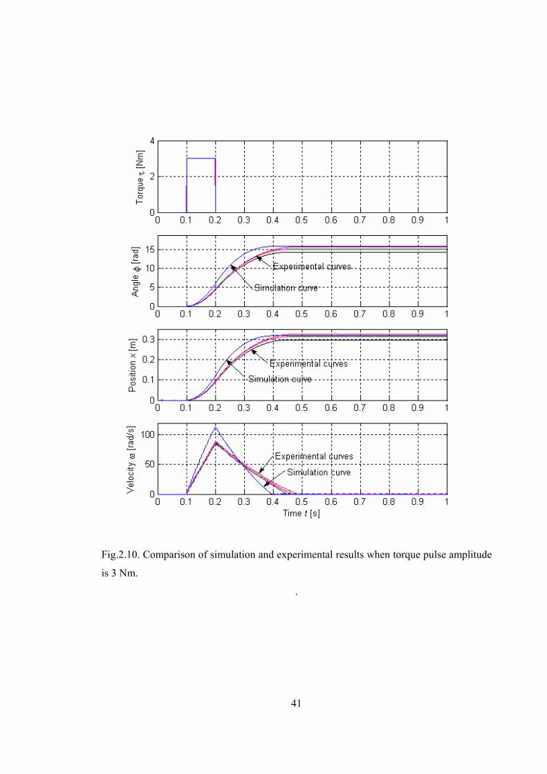
Fig.2.10. Comparison of simulation and experimental results when torque pulse amplitude

is 3 Nm.

.

42

Fig.2.11. Comparison of simulation and experimental results when torque pulse amplitude

is 2 Nm.

.

43

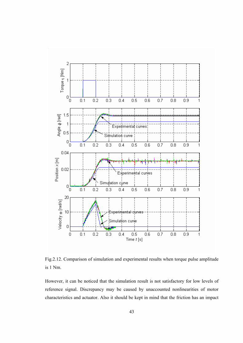
Fig.2.12. Comparison of simulation and experimental results when torque pulse amplitude

is 1 Nm.

However, it can be noticed that the simulation result is not satisfactory for low levels of

reference signal. Discrepancy may be caused by unaccounted nonlinearities of motor

characteristics and actuator. Also it should be kept in mind that the friction has an impact

44

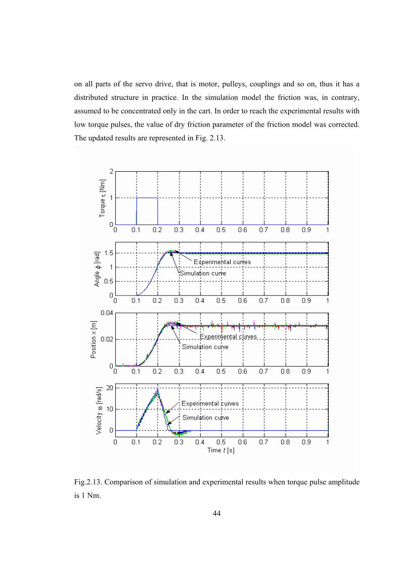
on all parts of the servo drive, that is motor, pulleys, couplings and so on, thus it has a

distributed structure in practice. In the simulation model the friction was, in contrary,

assumed to be concentrated only in the cart. In order to reach the experimental results with

low torque pulses, the value of dry friction parameter of the friction model was corrected.

The updated results are represented in Fig. 2.13.

Fig.2.13. Comparison of simulation and experimental results when torque pulse amplitude

is 1 Nm.

45

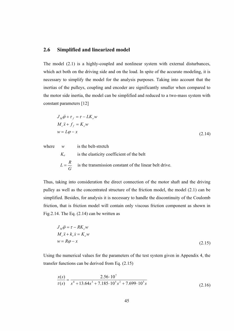
2.6 Simplified and linearized model

The model (2.1) is a highly-coupled and nonlinear system with external disturbances,

which act both on the driving side and on the load. In spite of the accurate modeling, it is

necessary to simplify the model for the analysis purposes. Taking into account that the

inertias of the pulleys, coupling and encoder are significantly smaller when compared to

the motor side inertia, the model can be simplified and reduced to a two-mass system with

constant parameters [12]

xLwwKfxM

wLKJ

efc

efM

−=

=+

−=+

ϕ

ττϕ&&

&&

(2.14)

where w is the belt-stretch

Ke is the elasticity coefficient of the belt

GRL = is the transmission constant of the linear belt drive.

Thus, taking into consideration the direct connection of the motor shaft and the driving

pulley as well as the concentrated structure of the friction model, the model (2.1) can be

simplified. Besides, for analysis it is necessary to handle the discontinuity of the Coulomb

friction, that is friction model will contain only viscous friction component as shown in

Fig.2.14. The Eq. (2.14) can be written as

xRwwKxkxM

wRKJ

evc

eM

−==+

−=

ϕ

τϕ&&&

&&

(2.15)

Using the numerical values for the parameters of the test system given in Appendix 4, the

transfer functions can be derived from Eq. (2.15)

ssssssx

52534

7

10699.710185.764.131056.2

)()(

⋅+⋅++⋅

=τ (2.16)

46

sssss

ss

52534

952

10699.710185.764.131028.110136.18333s

)()(

⋅+⋅++⋅+⋅+

=τϕ

(2.17)

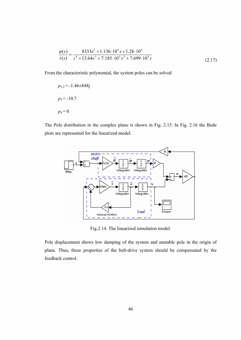
From the characteristic polynomial, the system poles can be solved

p1,2 = -1.46±848j

p3 = -10.7

p4 = 0

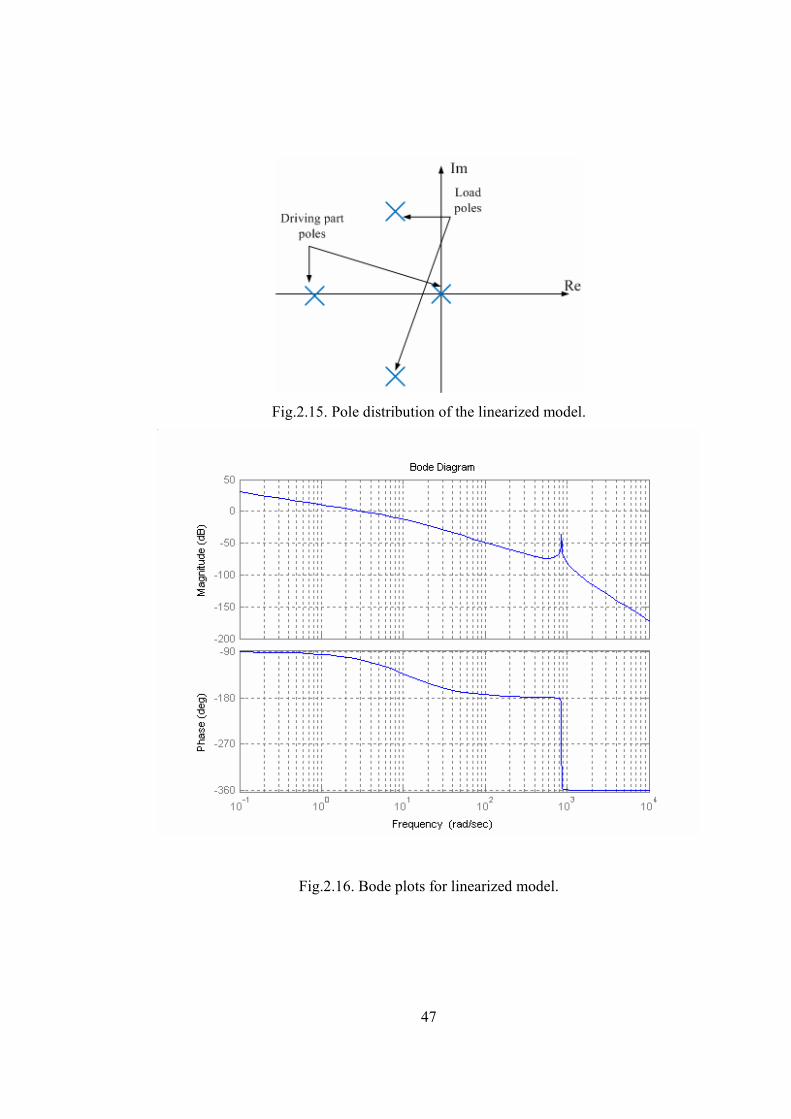
The Pole distribution in the complex plane is shown in Fig. 2.15. In Fig. 2.16 the Bode

plots are represented for the linearized model.

Fig.2.14. The linearized simulation model.

Pole displacement shows low damping of the system and unstable pole in the origin of

plane. Thus, these properties of the belt-drive system should be compensated by the

feedback control.

47

Fig.2.15. Pole distribution of the linearized model.

Fig.2.16. Bode plots for linearized model.

48

3 Control of the belt drive system

Modern industrial belt-drive products require operation of servodrives at high speed and

high accuracy. In addition, it is necessary to take into account frequency dependent

characteristic of force transmission in drive, which can prevent to achieve the required

performance. Moreover, in order to achieve rapid response and accurate position tracking

by control efforts vibrations in the mechanical drive system can occur due to resonance

frequencies. Besides friction effects in the system should be compensated in order to

achieve required performance of the system. It should be kept in mind, that friction model

include non-linear element which makes controller design more complicated. Thus,

control algorithm should be constructed in order to ensure wide frequency bandwidth of

the position servo system and compensate all friction affects in the system.

There are several methods in control theory allow the realization of such a control, with

which the high performance of linear belt-driven servomechanism under the plant

parameters variations, uncertain dynamics and disturbances can be reached. The most

useful methods to satisfy control requirements are briefly described below.

3.1 PID control

PID controllers are widely used in the process industries and commercial controller

hardware. [17] It is also used in a non-model based friction compensation [15], which can

eliminate stick-slip in high-stiffness systems. It is important to notice that the PID

controllers are widely used in servo drive systems based on cascade principle (such as in

Fig.1.2) as current, speed or position controllers.

A common structure of the PID controller is represented in Fig.3.1. As it can be noticed,

PID controller includes three terms:

49

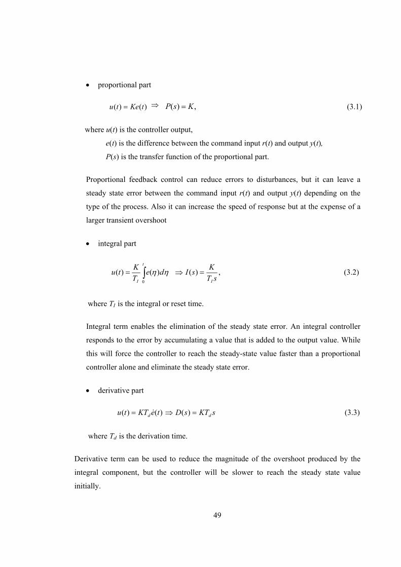
• proportional part

)()( tKetu = ⇒ ,)( KsP = (3.1)

where u(t) is the controller output,

e(t) is the difference between the command input r(t) and output y(t),

P(s) is the transfer function of the proportional part.

Proportional feedback control can reduce errors to disturbances, but it can leave a

steady state error between the command input r(t) and output y(t) depending on the

type of the process. Also it can increase the speed of response but at the expense of a

larger transient overshoot

• integral part

∫=t

I

deTKtu

0

)()( ηη ⇒ ,)(sT

KsII

= (3.2)

where TI is the integral or reset time.

Integral term enables the elimination of the steady state error. An integral controller

responds to the error by accumulating a value that is added to the output value. While

this will force the controller to reach the steady-state value faster than a proportional

controller alone and eliminate the steady state error.

• derivative part

)()( teKTtu d &= ⇒ sKTsD d=)( (3.3)

where Td is the derivation time.

Derivative term can be used to reduce the magnitude of the overshoot produced by the

integral component, but the controller will be slower to reach the steady state value

initially.

50

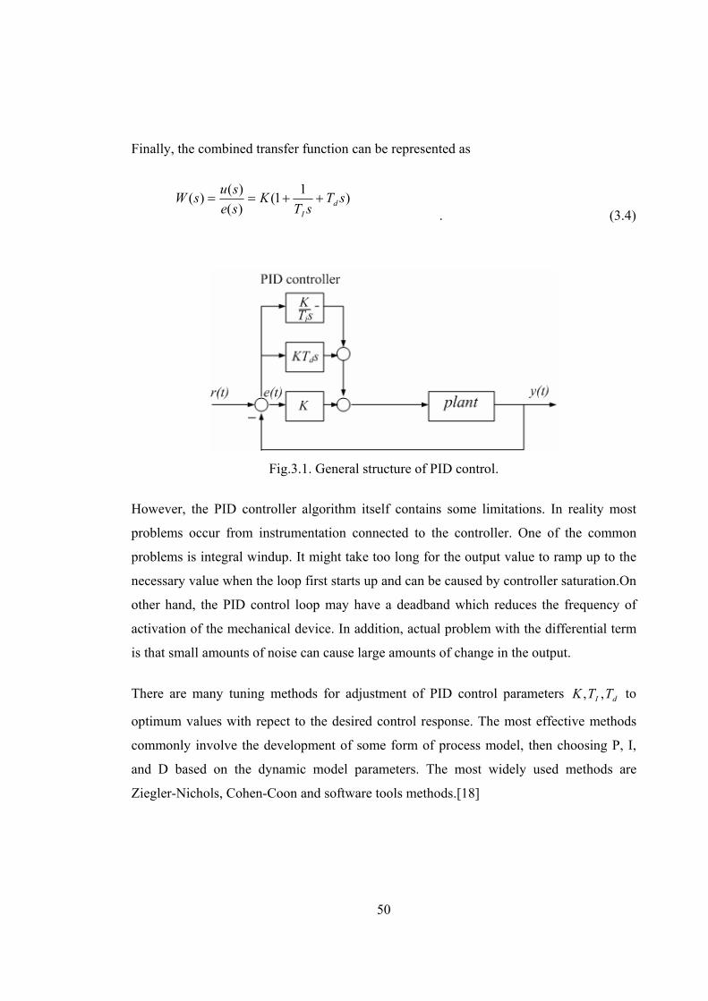
Finally, the combined transfer function can be represented as

)11(

)()()( sT

sTK

sesusW d

I

++== . (3.4)

Fig.3.1. General structure of PID control.

However, the PID controller algorithm itself contains some limitations. In reality most

problems occur from instrumentation connected to the controller. One of the common

problems is integral windup. It might take too long for the output value to ramp up to the

necessary value when the loop first starts up and can be caused by controller saturation.On

other hand, the PID control loop may have a deadband which reduces the frequency of

activation of the mechanical device. In addition, actual problem with the differential term

is that small amounts of noise can cause large amounts of change in the output.

There are many tuning methods for adjustment of PID control parameters dI TTK ,, to

optimum values with repect to the desired control response. The most effective methods

commonly involve the development of some form of process model, then choosing P, I,

and D based on the dynamic model parameters. The most widely used methods are

Ziegler-Nichols, Cohen-Coon and software tools methods.[18]

51

3.2 LQ-control

The most effective and widely used design technique of linear control system design is the

optimal linear quadratic regulator (LQR) design. [21] This technique is based on the state

space approach, namely on the pole placement philosophy. Selection of optimal pole

locations is very a complex task, because locations far from the origin may give the fast

dynamic response, but require large control efforts. LQ-method provides the balance

between good system response and the control effort required.

The idea of the LQ design method is to determine the control law of form u = -Kx, such

that the performance cost function

[ ]dtRuuQxxJ TT∫∞

+=0 (3.5)

is minimized for the system

,)()(

CxtyBuAxtx

=+=&

(3.6)

where x is the state vector

u is the control input

A, B and C are known system matrices

Q is the state weighting matrix

R is the control weighting matrix.

Components of the cost function characterize the integrated cost of the control: the

quadratic form QxxT represents penalty on the deviation of the state x from the origin and

the term RuuT represents the control effort. Thus, weighting matrix Q specifies the

importance of the various components of the state vector relative to each other and by

choice of Q matrix the different control purposes can be achieved. On the other hand, the

control weighting matrix R should be selected in order to avoid saturation of control signal

and its consequences because the closed-loop behavior is not predictable when the control

52

signal is saturated. It should be mentioned that weighting matrices Q and R are

non-negative definite symmetric matrices; otherwise the LQ-algorithm will

not work. However, the relation between the matrices Q and R and the behavior of the

closed-loop system depending on A and B matrices is quite complex. Selection of the

weighting matrices to achieve control objectives is therefore a complex task for control

system designers, but it is easy to calculate the optimal control gains with widely available

computer software. [22]

The LQ-controller has several advantages. It is applicable to multivariable and time-

varying systems. Moreover, by means of changing the relative costs between the elements

in weighting matrices a compromise between the speed of recovery and the magnitudes of

control signals can be made.

3.3 Adaptive control

Definition of the term adaptive is “to modify according to changing circumstances”, thus

almost all adaptive control systems modifies themselves under changing cicumstances.

Generally, the subject of adaptive control is design control algorithm which somehow

automatically redesigns itself as plant changes, because parameter variations of a control

system can have impact on the perfomance and stability. As result, adaptive control is

required:

• at a important uncertainty of the plant’s parameters and operating conditions,

• when dynamic properties of the plant vary in wide range in unknown way,

• when initial information is not enough for design of control system with optimal or

specified perfomance. [24]

Thus, adaptive technique can be appropriate for linear belt-drive taking into account

uncertinty of dry friction as well as non-linearity of elasticity of the belt.

53

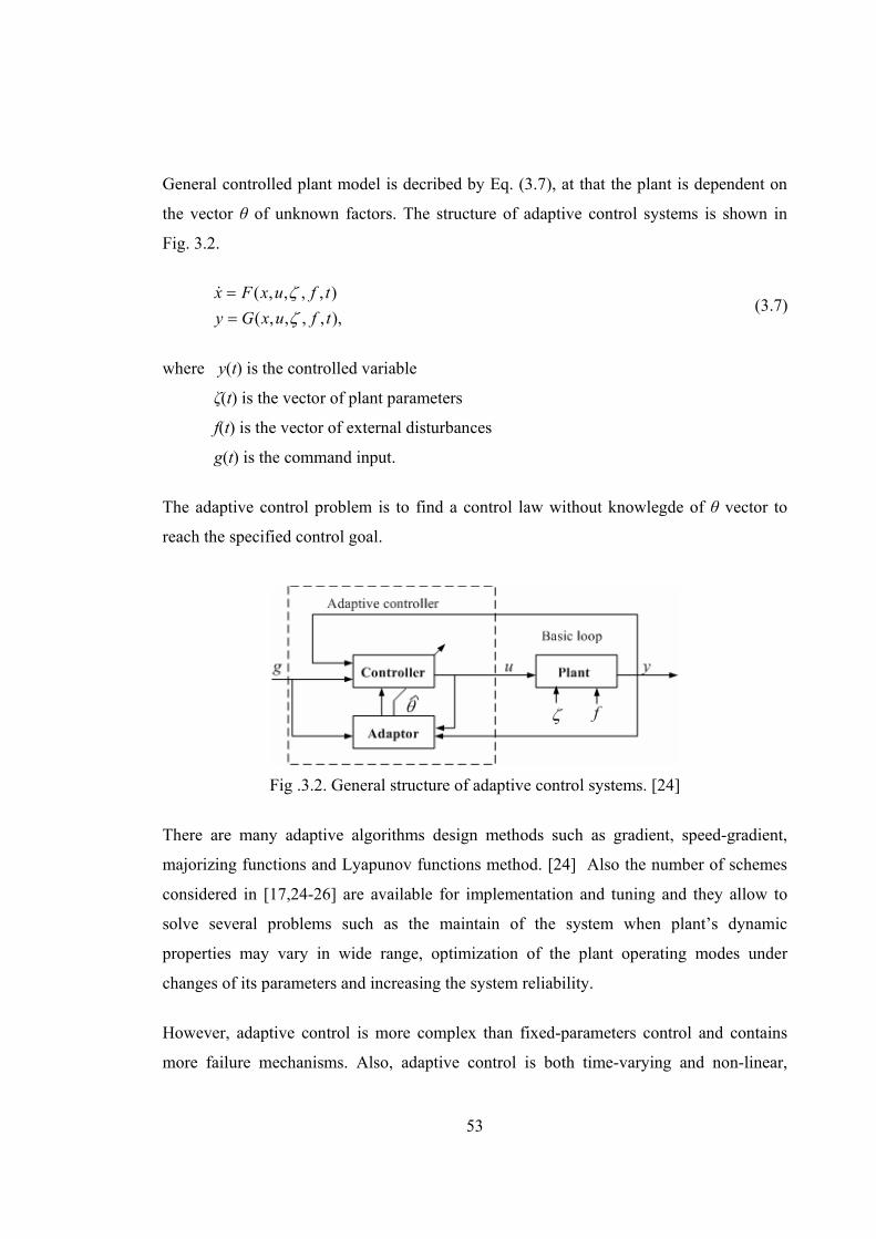
General controlled plant model is decribed by Eq. (3.7), at that the plant is dependent on

the vector θ of unknown factors. The structure of adaptive control systems is shown in

Fig. 3.2.

),,,,,(),,,,(

tfuxGytfuxFx

ζζ

==&

(3.7)

where y(t) is the controlled variable

ζ(t) is the vector of plant parameters

f(t) is the vector of external disturbances

g(t) is the command input.

The adaptive control problem is to find a control law without knowlegde of θ vector to

reach the specified control goal.

Fig .3.2. General structure of adaptive control systems. [24]

There are many adaptive algorithms design methods such as gradient, speed-gradient,

majorizing functions and Lyapunov functions method. [24] Also the number of schemes

considered in [17,24-26] are available for implementation and tuning and they allow to

solve several problems such as the maintain of the system when plant’s dynamic

properties may vary in wide range, optimization of the plant operating modes under

changes of its parameters and increasing the system reliability.

However, adaptive control is more complex than fixed-parameters control and contains

more failure mechanisms. Also, adaptive control is both time-varying and non-linear,

54

increasing the difficulty of stability and perfomance analysis. Many of the adaptive

algorithms require also large amount of computation. In addition, the costs of the

controller and its implementation increase with the complexity of the design.

3.4 Sliding mode control (SMC)

Modeling inaccuracies such as friction and belt elasticity can have negative effects on

nonlinear control systems. One of the most important approaches dealing with model

uncertainties is sliding mode control.

Sliding mode control is a special type of variable structure control systems. Variable

structure control systems (VSCS) are characterized by appropriate feedback control laws

and switching function, which selects a particular feedback control in accordance with the

systems behavior. In the sliding mode control, VSCS are made to attract the system states

to a sliding surface. When the sliding surface is reached, the sliding mode control saves

the states on the close neighborhood of the sliding surface.

The design of the sliding mode control contains two parts. The first part includes the

design of a switching function in order to satisfy the sliding motion design specifications.

The second task is the selection of a control law, which ensures the switching surface to

attract the system state.

For a system

),,()()( uxtftButAxx ++=& , (3.8)

where the function f(t,x,u) is assumed to be unknown but bounded by known functions of

the state the sliding mode equation is given as

0)( 112211 =++++= −− nnn xxsxsxsx Kσ . (3.9)

The condition of existence of sliding mode should be satisfied in accordance with the

theorem

55

0<σσ & for ∀ t t∆∈ . (3.10)

Thus, the control law for system operating in the sliding mode is

=−

+

),(),(

),(xuxu

txu00

<>

σσ

forfor

(3.11)

The example of sliding mode of a 2nd order dynamic system with Coulomb friction is

shown in Fig. 3.3.

Fig.3.3. Sliding mode in dynamic system. [24]

The main advantages of sliding mode control are that the dynamic behavior of the system

can be selected by the proper choice of the sliding function and that the closed loop

response becomes totally insensitive to some appropriate uncertainties. This principle

spreads to model parameter uncertainties, disturbances and non-linearities that are

bounded.

Sliding mode control has a discontinuous structure. Therefore it creates some difficulties

because the infinite frequency of the control effort is required at sliding surface to save the

system states on the sliding surface. Thus, sliding mode control is not recommended to be

56

use in mechanical systems due to fast wearing of the parts. Filtering and continuous

approximation of the control law can be employed to prevent that problem, but the

robustness properties of the sliding mode control is then lost. [27]

3.5 Advantages and disadvantages of different control techniques

The main properties of the considered control techniques are listed in Table 3.1. It can be

seen that all methods have advantages and disadvantages. The choice of appropriate

control for the system is always a compromise between the quality and the costs.

However, it should be mentioned that the more complex structure increases the amount of

mechanisms which can carry an additional risks for the system. Therefore the compromise

can be found among simple techniques.

57

Table 3.1. The benefits and drawbacks of different control techniques.

benefits drawbacks

PID control - simple structure

- automatic tuning

- integral windup

- noise from derivative term

- deadband which reduces the

frequency of activation

LQ control - automatic calculation of control

law

- automatic tuning

- simple structure

- difficulties in selection of

weighting matrices

- linearization of the model is

required

- feedback from measured or

estimated state variables is needed

Adaptive

control

- maintain of the system when

plant’s dynamic properties may

vary in wide range,

- optimization of the plant

operating modes under changes of

its parameters

- increasing the system reliability

- large amount of computation

- high price

- diffucult to design

- contains much failure

mechanisms

SMC - selection of system dynamic by

switching function

- unsensetivity to particular

uncertainties

- infinite frequency of control

efforts is required

- not recommended in mechanical

systems

58

4 Control synthesis for the position tracking

The simplest way to construct a control method satisfying the specified control

requirements is using MATLAB® instruments. It is not necessary to simplify or linearized

the model for the control purposes. Thus, for the realization of the closed-loop system, a

PID controller with automatic tuning using the Nonlinear Control Design (NCD) Blockset

and the cart position feedback was chosen.

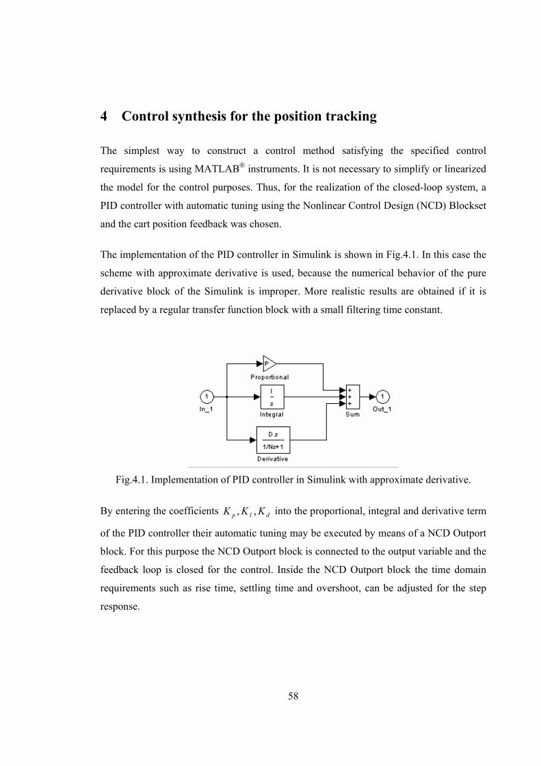
The implementation of the PID controller in Simulink is shown in Fig.4.1. In this case the

scheme with approximate derivative is used, because the numerical behavior of the pure

derivative block of the Simulink is improper. More realistic results are obtained if it is

replaced by a regular transfer function block with a small filtering time constant.

Fig.4.1. Implementation of PID controller in Simulink with approximate derivative.

By entering the coefficients dIp KKK ,, into the proportional, integral and derivative term

of the PID controller their automatic tuning may be executed by means of a NCD Outport

block. For this purpose the NCD Outport block is connected to the output variable and the

feedback loop is closed for the control. Inside the NCD Outport block the time domain

requirements such as rise time, settling time and overshoot, can be adjusted for the step

response.

59

The NCD Blockset automatically converts the adjusted time domain constraints into a

constrained optimization problem and then solves the problem using state-of-the-art

optimization routines from the Optimization Toolbox. The constrained optimization

problem interpreted by the NCD Blockset iteratively calls for simulations of the Simulink

system, compares the results of the simulations with the constraint objectives, and uses

gradient methods to adjust the tunable parameters to reach the objectives. The NCD

Blockset allows solving control problem with uncertainty in the plant dynamics, conduct

Monte Carlo simulations, and specify the lower and upper limits of the tunable variables.

[19]

Two cases o the automated PID tuning are presented below.

4.1 Automatic PID tuning for accurate position control

In accodance with the control requirements the step response must satisfy the following

requirements:

• Zero steady state error

• Damping more than 0.8

• Settling time as small as possible without extensive saturation of the actuator

Fig.4.2. Block scheme for tuning PID regulator parameters with help NCD Outport block

60

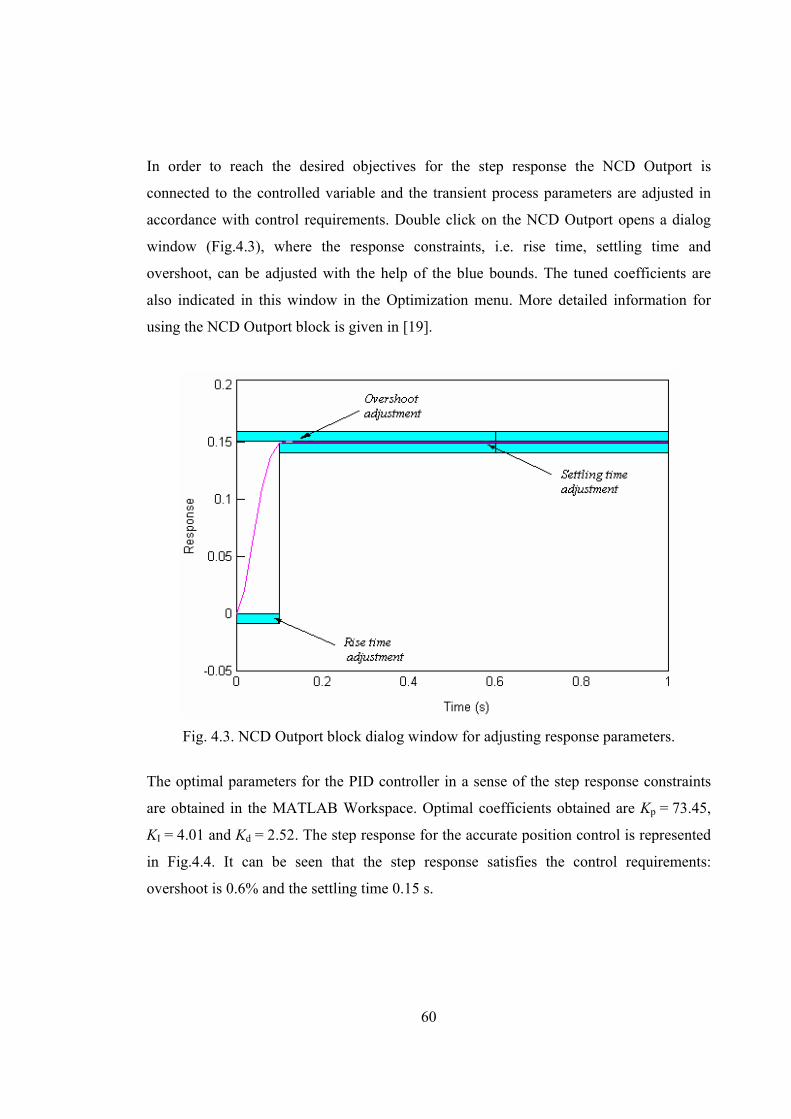
In order to reach the desired objectives for the step response the NCD Outport is

connected to the controlled variable and the transient process parameters are adjusted in

accordance with control requirements. Double click on the NCD Outport opens a dialog

window (Fig.4.3), where the response constraints, i.e. rise time, settling time and

overshoot, can be adjusted with the help of the blue bounds. The tuned coefficients are

also indicated in this window in the Optimization menu. More detailed information for

using the NCD Outport block is given in [19].

Fig. 4.3. NCD Outport block dialog window for adjusting response parameters.

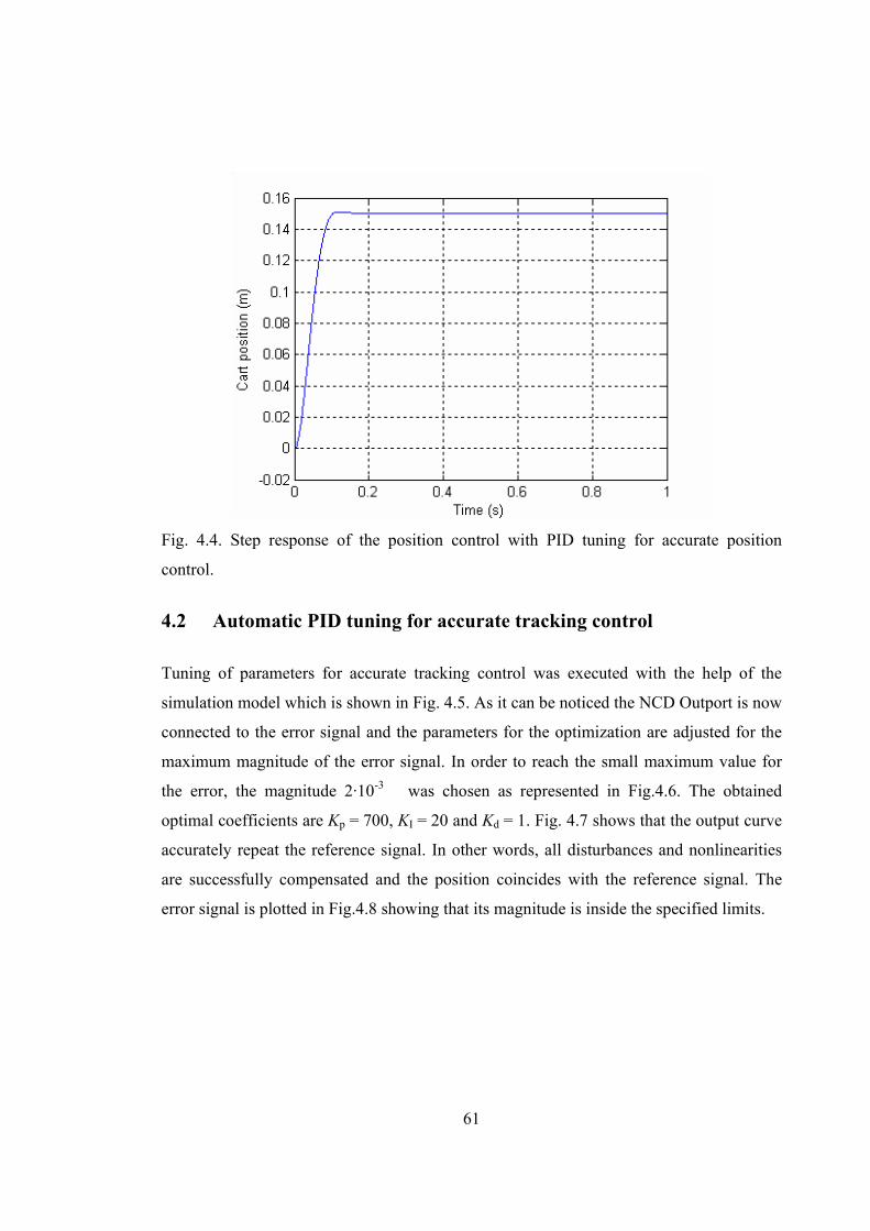
The optimal parameters for the PID controller in a sense of the step response constraints

are obtained in the MATLAB Workspace. Optimal coefficients obtained are Kp = 73.45,

KI = 4.01 and Kd = 2.52. The step response for the accurate position control is represented

in Fig.4.4. It can be seen that the step response satisfies the control requirements:

overshoot is 0.6% and the settling time 0.15 s.

61

Fig. 4.4. Step response of the position control with PID tuning for accurate position

control.

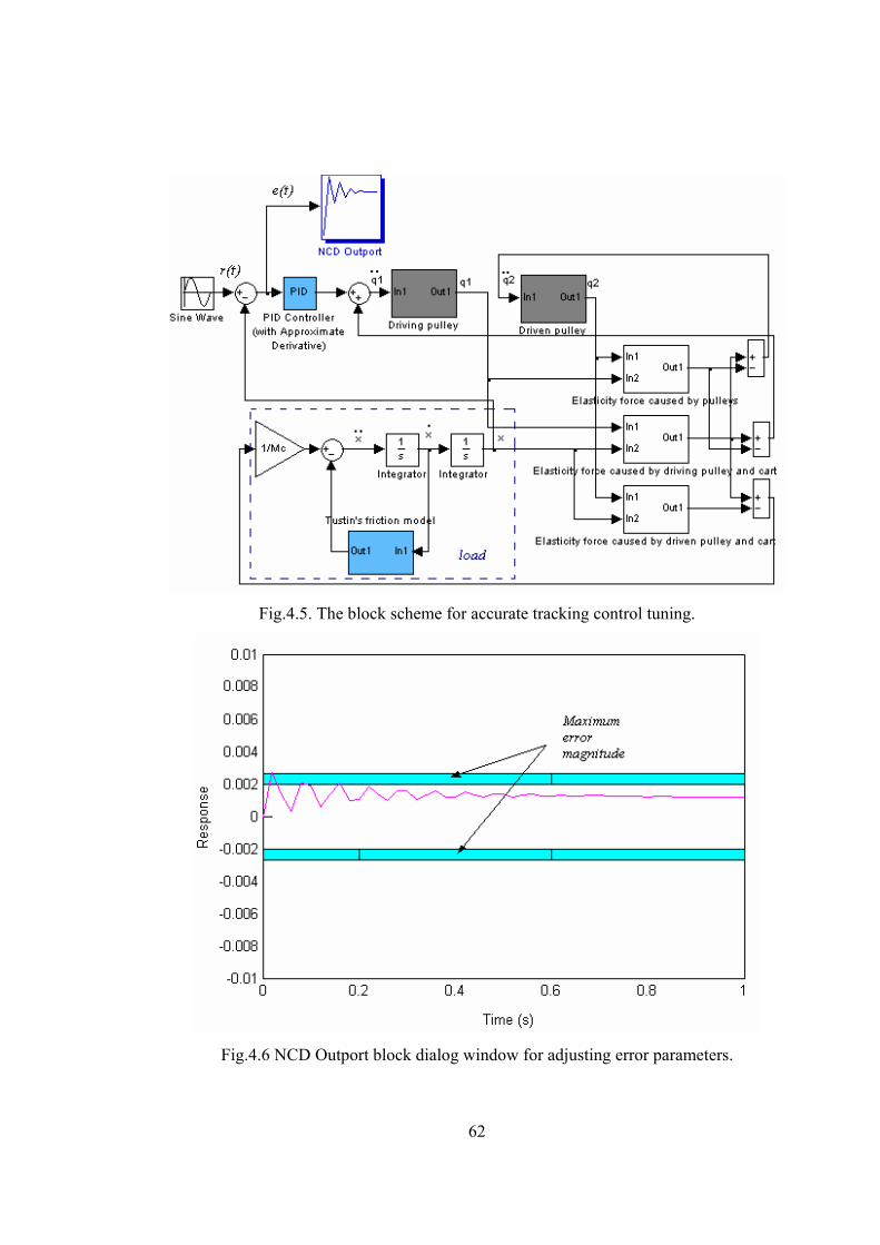
4.2 Automatic PID tuning for accurate tracking control

Tuning of parameters for accurate tracking control was executed with the help of the

simulation model which is shown in Fig. 4.5. As it can be noticed the NCD Outport is now

connected to the error signal and the parameters for the optimization are adjusted for the

maximum magnitude of the error signal. In order to reach the small maximum value for

the error, the magnitude 2·10-3 was chosen as represented in Fig.4.6. The obtained

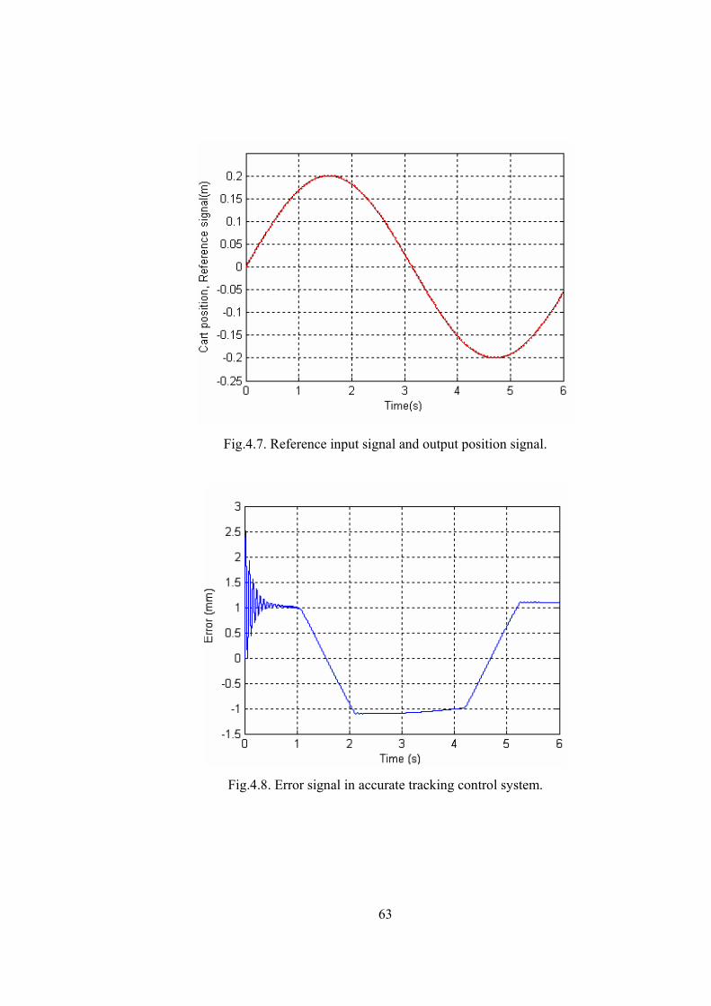
optimal coefficients are Kp = 700, KI = 20 and Kd = 1. Fig. 4.7 shows that the output curve

accurately repeat the reference signal. In other words, all disturbances and nonlinearities

are successfully compensated and the position coincides with the reference signal. The

error signal is plotted in Fig.4.8 showing that its magnitude is inside the specified limits.

62

Fig.4.5. The block scheme for accurate tracking control tuning.

Fig.4.6 NCD Outport block dialog window for adjusting error parameters.

63

Fig.4.7. Reference input signal and output position signal.

Fig.4.8. Error signal in accurate tracking control system.

64

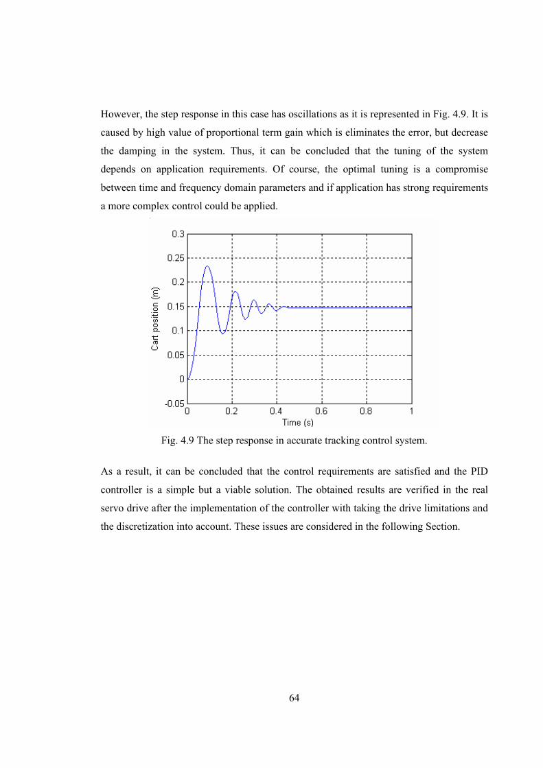
However, the step response in this case has oscillations as it is represented in Fig. 4.9. It is

caused by high value of proportional term gain which is eliminates the error, but decrease

the damping in the system. Thus, it can be concluded that the tuning of the system

depends on application requirements. Of course, the optimal tuning is a compromise

between time and frequency domain parameters and if application has strong requirements

a more complex control could be applied.

Fig. 4.9 The step response in accurate tracking control system.

As a result, it can be concluded that the control requirements are satisfied and the PID

controller is a simple but a viable solution. The obtained results are verified in the real

servo drive after the implementation of the controller with taking the drive limitations and

the discretization into account. These issues are considered in the following Section.

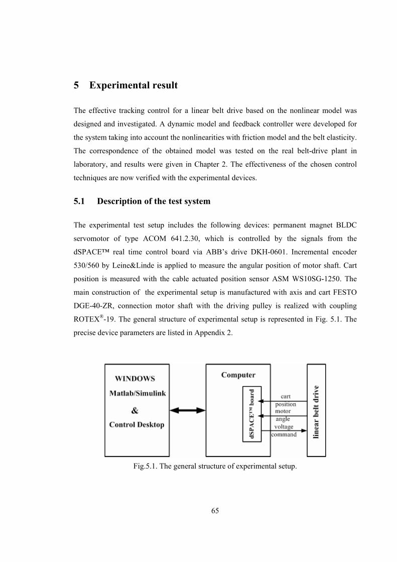
65

5 Experimental result

The effective tracking control for a linear belt drive based on the nonlinear model was

designed and investigated. A dynamic model and feedback controller were developed for

the system taking into account the nonlinearities with friction model and the belt elasticity.

The correspondence of the obtained model was tested on the real belt-drive plant in

laboratory, and results were given in Chapter 2. The effectiveness of the chosen control

techniques are now verified with the experimental devices.

5.1 Description of the test system

The experimental test setup includes the following devices: permanent magnet BLDC

servomotor of type ACOM 641.2.30, which is controlled by the signals from the

dSPACE™ real time control board via ABB’s drive DKH-0601. Incremental encoder

530/560 by Leine&Linde is applied to measure the angular position of motor shaft. Cart

position is measured with the cable actuated position sensor ASM WS10SG-1250. The

main construction of the experimental setup is manufactured with axis and cart FESTO

DGE-40-ZR, connection motor shaft with the driving pulley is realized with coupling

ROTEX®-19. The general structure of experimental setup is represented in Fig. 5.1. The

precise device parameters are listed in Appendix 2.

Fig.5.1. The general structure of experimental setup.

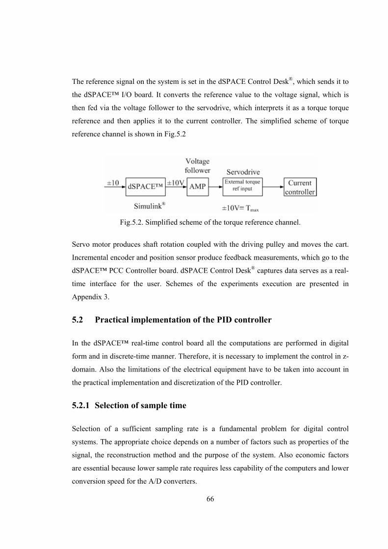
66

The reference signal on the system is set in the dSPACE Control Desk®, which sends it to

the dSPACE™ I/O board. It converts the reference value to the voltage signal, which is

then fed via the voltage follower to the servodrive, which interprets it as a torque torque

reference and then applies it to the current controller. The simplified scheme of torque

reference channel is shown in Fig.5.2

Fig.5.2. Simplified scheme of the torque reference channel.

Servo motor produces shaft rotation coupled with the driving pulley and moves the cart.

Incremental encoder and position sensor produce feedback measurements, which go to the

dSPACE™ PCC Controller board. dSPACE Control Desk® captures data serves as a real-

time interface for the user. Schemes of the experiments execution are presented in

Appendix 3.

5.2 Practical implementation of the PID controller

In the dSPACE™ real-time control board all the computations are performed in digital

form and in discrete-time manner. Therefore, it is necessary to implement the control in z-

domain. Also the limitations of the electrical equipment have to be taken into account in

the practical implementation and discretization of the PID controller.

5.2.1 Selection of sample time

Selection of a sufficient sampling rate is a fundamental problem for digital control

systems. The appropriate choice depends on a number of factors such as properties of the

signal, the reconstruction method and the purpose of the system. Also economic factors

are essential because lower sample rate requires less capability of the computers and lower

conversion speed for the A/D converters.

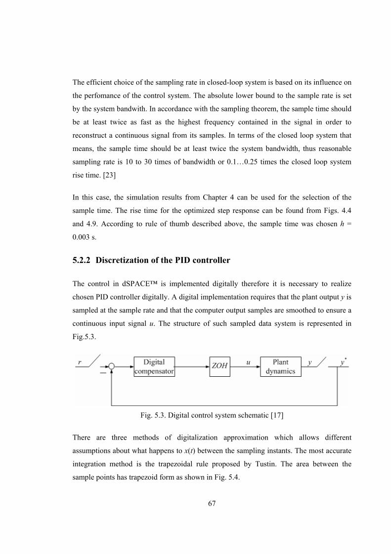
67

The efficient choice of the sampling rate in closed-loop system is based on its influence on

the perfomance of the control system. The absolute lower bound to the sample rate is set

by the system bandwith. In accordance with the sampling theorem, the sample time should

be at least twice as fast as the highest frequency contained in the signal in order to

reconstruct a continuous signal from its samples. In terms of the closed loop system that

means, the sample time should be at least twice the system bandwidth, thus reasonable

sampling rate is 10 to 30 times of bandwidth or 0.1…0.25 times the closed loop system

rise time. [23]

In this case, the simulation results from Chapter 4 can be used for the selection of the

sample time. The rise time for the optimized step response can be found from Figs. 4.4

and 4.9. According to rule of thumb described above, the sample time was chosen h =

0.003 s.

5.2.2 Discretization of the PID controller

The control in dSPACE™ is implemented digitally therefore it is necessary to realize

chosen PID controller digitally. A digital implementation requires that the plant output y is

sampled at the sample rate and that the computer output samples are smoothed to ensure a

continuous input signal u. The structure of such sampled data system is represented in

Fig.5.3.

Fig. 5.3. Digital control system schematic [17]

There are three methods of digitalization approximation which allows different

assumptions about what happens to x(t) between the sampling instants. The most accurate

integration method is the trapezoidal rule proposed by Tustin. The area between the

sample points has trapezoid form as shown in Fig. 5.4.

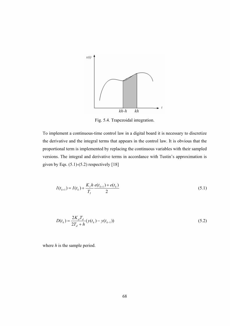
68

Fig. 5.4. Trapezoidal integration.

To implement a continuous-time control law in a digital board it is necessary to discretize

the derivative and the integral terms that appears in the control law. It is obvious that the

proportional term is implemented by replacing the continuous variables with their sampled

versions. The integral and derivative terms in accordance with Tustin’s approximation is

given by Eqs. (5.1)-(5.2) respectively [18]

2)()(

)()( 11

kk

I

Ikk

teteT

hKtItI+

+= ++ (5.1)

))()((22

)( 1−−+

= kkd

ddk tyty

hTTK

tD (5.2)

where h is the sample period.

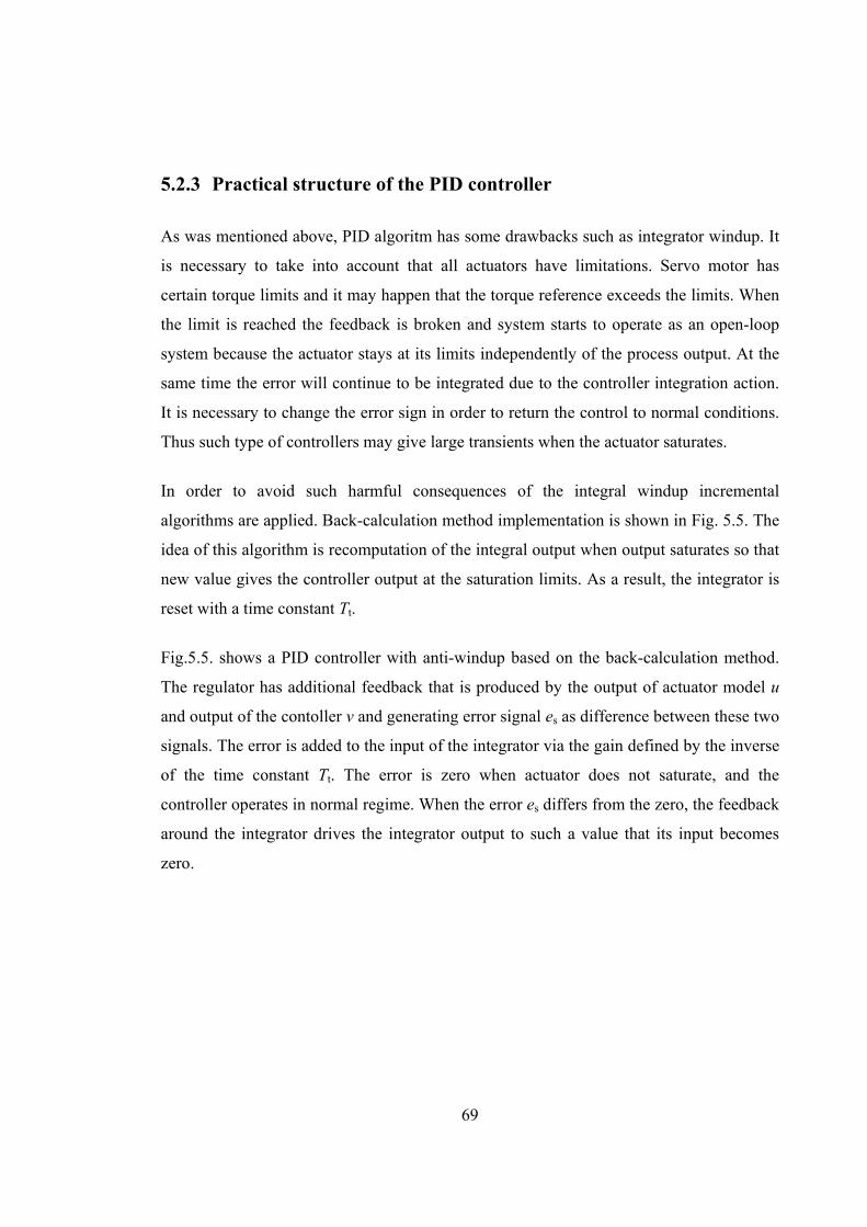
69

5.2.3 Practical structure of the PID controller

As was mentioned above, PID algoritm has some drawbacks such as integrator windup. It

is necessary to take into account that all actuators have limitations. Servo motor has

certain torque limits and it may happen that the torque reference exceeds the limits. When

the limit is reached the feedback is broken and system starts to operate as an open-loop

system because the actuator stays at its limits independently of the process output. At the

same time the error will continue to be integrated due to the controller integration action.

It is necessary to change the error sign in order to return the control to normal conditions.

Thus such type of controllers may give large transients when the actuator saturates.

In order to avoid such harmful consequences of the integral windup incremental

algorithms are applied. Back-calculation method implementation is shown in Fig. 5.5. The

idea of this algorithm is recomputation of the integral output when output saturates so that

new value gives the controller output at the saturation limits. As a result, the integrator is

reset with a time constant Tt.

Fig.5.5. shows a PID controller with anti-windup based on the back-calculation method.

The regulator has additional feedback that is produced by the output of actuator model u

and output of the contoller v and generating error signal es as difference between these two

signals. The error is added to the input of the integrator via the gain defined by the inverse

of the time constant Tt. The error is zero when actuator does not saturate, and the

controller operates in normal regime. When the error es differs from the zero, the feedback

around the integrator drives the integrator output to such a value that its input becomes

zero.

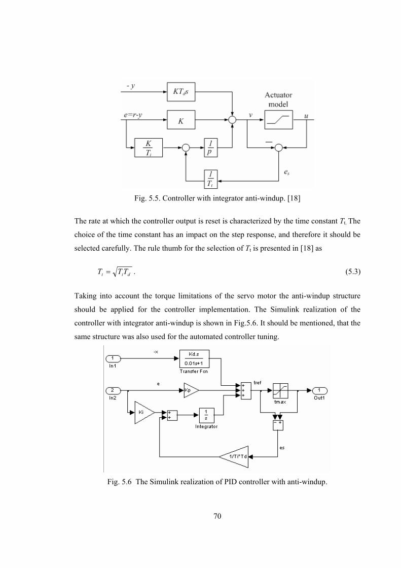
70

Fig. 5.5. Controller with integrator anti-windup. [18]

The rate at which the controller output is reset is characterized by the time constant Tt. The

choice of the time constant has an impact on the step response, and therefore it should be

selected carefully. The rule thumb for the selection of Tt is presented in [18] as

dit TTT = . (5.3)

Taking into account the torque limitations of the servo motor the anti-windup structure

should be applied for the controller implementation. The Simulink realization of the

controller with integrator anti-windup is shown in Fig.5.6. It should be mentioned, that the

same structure was also used for the automated controller tuning.

Fig. 5.6 The Simulink realization of PID controller with anti-windup.

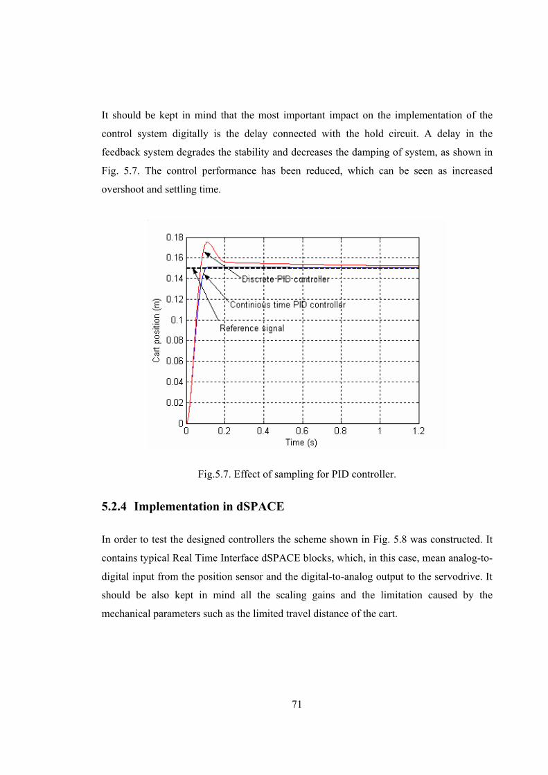
71

It should be kept in mind that the most important impact on the implementation of the

control system digitally is the delay connected with the hold circuit. A delay in the

feedback system degrades the stability and decreases the damping of system, as shown in

Fig. 5.7. The control performance has been reduced, which can be seen as increased

overshoot and settling time.

Fig.5.7. Effect of sampling for PID controller.

5.2.4 Implementation in dSPACE

In order to test the designed controllers the scheme shown in Fig. 5.8 was constructed. It

contains typical Real Time Interface dSPACE blocks, which, in this case, mean analog-to-

digital input from the position sensor and the digital-to-analog output to the servodrive. It

should be also kept in mind all the scaling gains and the limitation caused by the

mechanical parameters such as the limited travel distance of the cart.

72

Fig. 5.8. Scheme for PID control testing.

Designed PID controller is embedded to the position feedback. The reference signal in this

scheme is applied as position deviation. In such a way, the response of the real test setup

can be measured to the different input signals. The measurement results are shown in the

next part and compared with the corresponding simulation curves.

5.3 Comparison of the simulation and measurement results

The measurement and simulation results are given in Figs. 5.9-5.10 for the position

control and in Fig.(5.11) for the tracking control. As it can be observed from the figures,

the automatic tuning gives otherwise acceptable response except the tail of the response,

which approaches the reference value very slowly. This is probably caused by the fact that

the controller cancels slow process poles with relatively large integration time constant

(small integral part gain) in order to get sufficient response to the setpoint changes. On the

other hand this results that the controller has a rather poor rejection of the constant

disturbances such as the stiction in this system. Fig. 5.11 shows also that the offset error

elimination by position tracking control is not enough effective, because it takes several

seconds to decay. The position error has also intolerably large value for high precision

systems. It can beconcluded that automatic tuning can be used only for pre-tuning of the

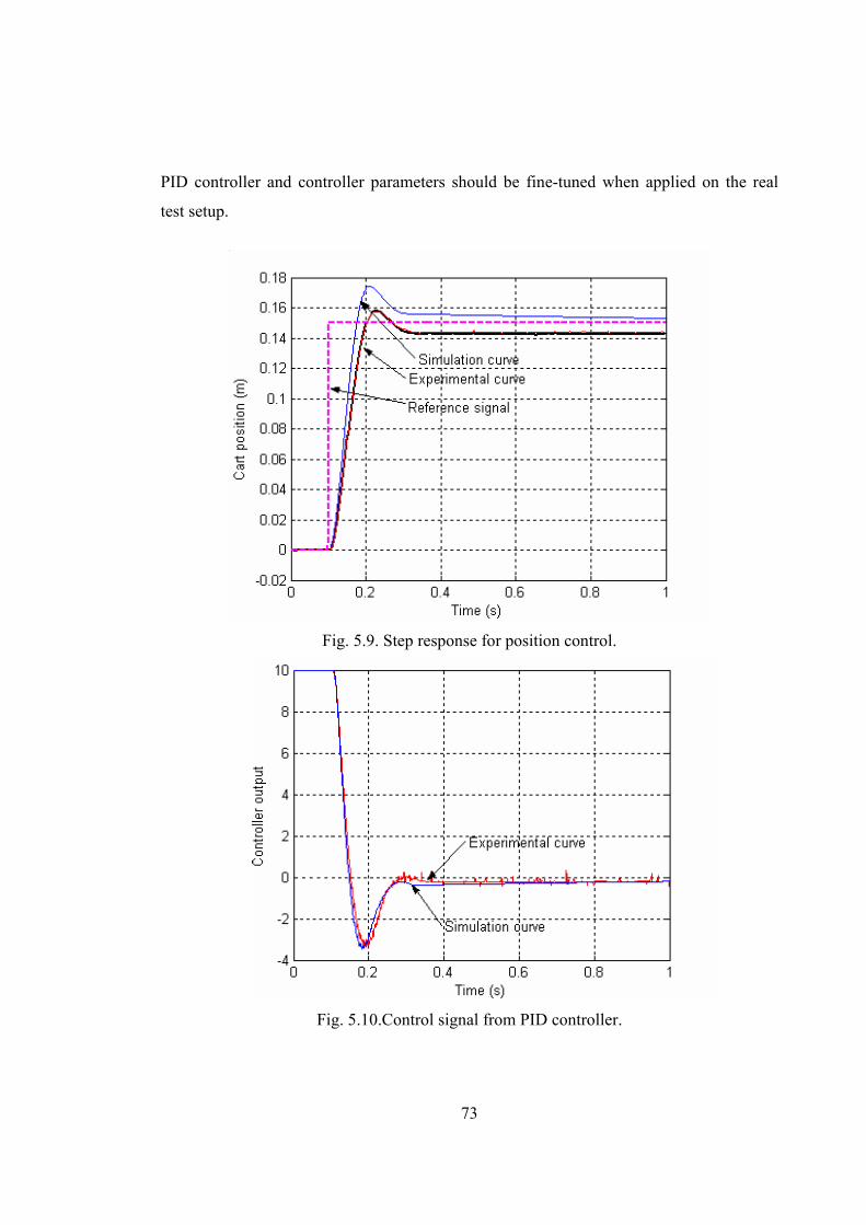
73

PID controller and controller parameters should be fine-tuned when applied on the real

test setup.

Fig. 5.9. Step response for position control.

Fig. 5.10.Control signal from PID controller.

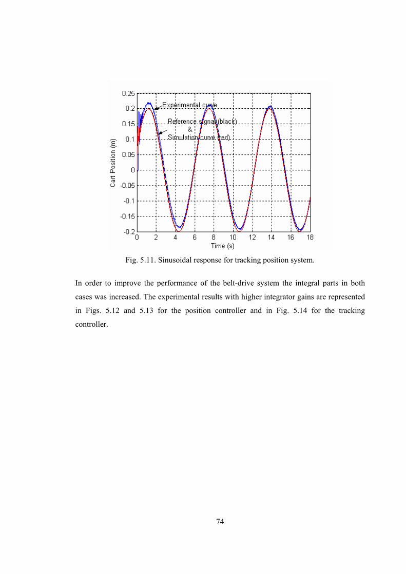
74

Fig. 5.11. Sinusoidal response for tracking position system.

In order to improve the performance of the belt-drive system the integral parts in both

cases was increased. The experimental results with higher integrator gains are represented

in Figs. 5.12 and 5.13 for the position controller and in Fig. 5.14 for the tracking

controller.

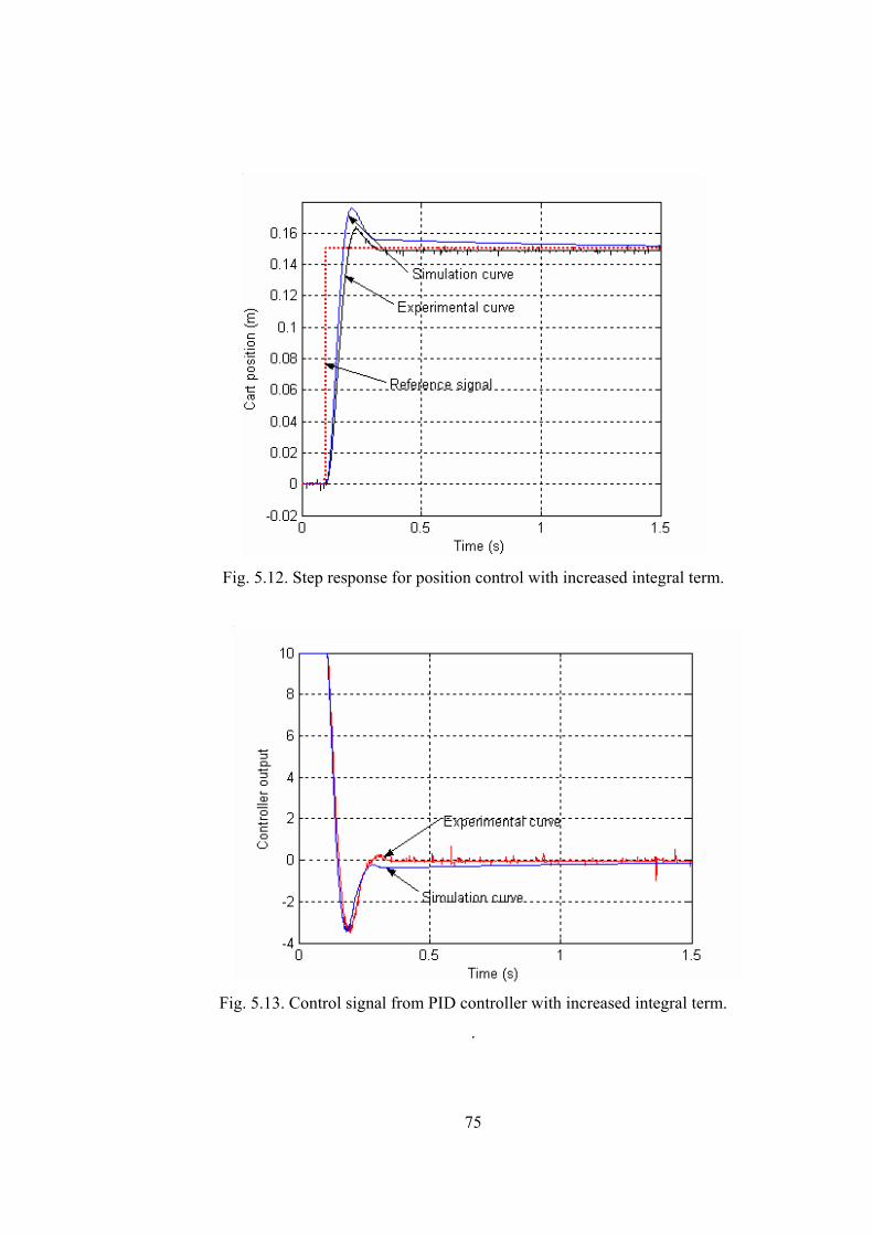
75

Fig. 5.12. Step response for position control with increased integral term.

Fig. 5.13. Control signal from PID controller with increased integral term.

.

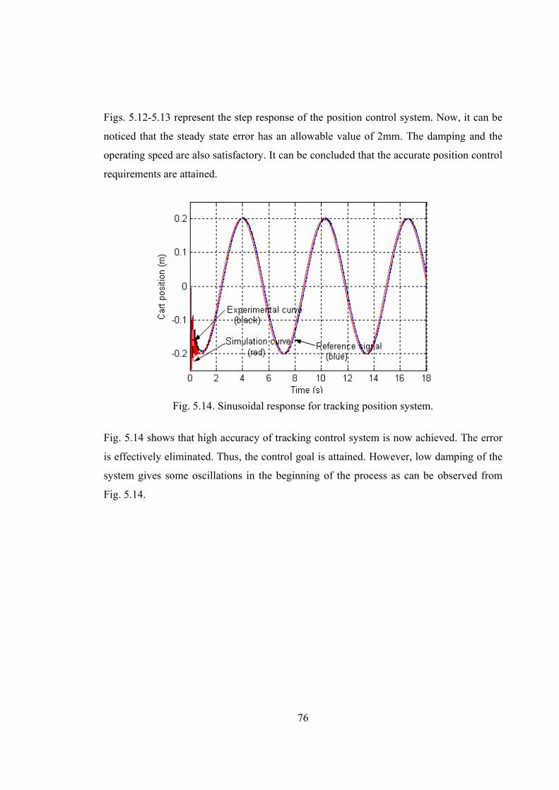
76

Figs. 5.12-5.13 represent the step response of the position control system. Now, it can be

noticed that the steady state error has an allowable value of 2mm. The damping and the

operating speed are also satisfactory. It can be concluded that the accurate position control

requirements are attained.

Fig. 5.14. Sinusoidal response for tracking position system.

Fig. 5.14 shows that high accuracy of tracking control system is now achieved. The error

is effectively eliminated. Thus, the control goal is attained. However, low damping of the

system gives some oscillations in the beginning of the process as can be observed from

Fig. 5.14.

77

6 Conclusions

As result of the work a model of the belt drive system and its PID control was developed.

The designed model describes the system behavior with adequate accuracy. Friction and

belt elasticity phenomena impact was taken into account in the developed model. The

correspondence of the model was demonstrated by experimental tests.

The PID control based on the position feedback was developed. This control was applied

to the designed dynamic model to show its effectiveness by simulations. Using the

developed model the pretuning of the controller with the help of MATLAB® instruments

can be performed.

Also the practical structure of PID control was constructed with taking into account the

limitations of the actuator. In addition, the discretization of the PID controller was made

for implementation it to the dSPACE™ system. The effectiveness of the developed

controllers was proved by experimental tests.

The developed position control system ensures allowable error value. Also the damping

and the operating speed of the closed loop system are satisfactory. As a conclusion, the

specified position control requirements were attained.

High accuracy of the belt drive system is achieved with the help of tracking controller.

The position error is effectively eliminated. However, low damping of the system gives

oscillations in the beginning of the process, which may present a limiting factor in some

practical application. The position tracking control requires impovement in order to avoid

the oscillations in the step response.

78

References:

[1] “Application Examples”: Parker Hannifin Corporation. 16 April 2007

<http://www.parkermotion.com/catalog_eng_ref.htm>

[2] Kerrkanen K., 2006. Dynamic analysis of belt-drives using the absolute nodal

coordinate formulation. /PhD work Lappeenranta University of Technology. ISBN 952-

214-193-3

[3] Hungles, A., 2003. Electric motors and drives: Fundamentals, types and applications.-

Printed by Newnes, Manchester. ISBN 0-7506-1741-1

[4] Younkin, G., 2003. Industrial servo control systems: Fundamentals and applications.

[5] Drury, B., 2001. The Control Techniques Drives and Controls Handbook, Published

by the Institution of Electrical Engineers, London. ISBN 0-85296-793-4

[6] Crowder R. M., 1995. Electric drives and their controls, Clarendon Press, Oxford.

ISBN 0-19-859371-6

[7] Toshihiro, S., Tsuneo, K., 2004. Motor drive technology: History and visions for the

future. 35th Annual IEEE Power Electronics Specialists Conference, p.2-9.

[8] Puranen, J., Induction motor versus permanent magnet synchronous motor in motion

control applications: a comparative study. / PhD work Lappeenranta University of

Technology. ISBN 952-214-296-4

[9] Mikerov A.G., Djankhotov V.V., 2002. Small electrical machines and drives. Saint-

Petersburg Electrotechnical University “LETI”, Russia

[10] Pyrhonen J., 2006. Electrical Drives 2006/2007, Lecture notes, LUT, Finland.

79

[11] Barret J., Harned T., Monnich J. Linear motor basics. Parker Hannifin Corporation.

[12] Hace, A., Jezernik, K., Sabanovic, A., SMC with disturbance observer for a linear

belt-drive, IEEE ISIE 2005, June 20-23, Dubrovnik, Croatia.

[13] Serway R.A., 1982.Physics: For scientists and engineers. ISBN 0-03-057903-1

[14] Armstrong –Helouvry, B, 1991. Control of machines with friction. Published by

Kluwer Academic Publishers, Boston.

[15] Yu-Feng Li, Motion, 1999. Control Subject to Nonlinearities and Flexibility (A

Overview based on friction and flexibility compensation), Technical report, Department of

Machine Design, Royal Institute of Technology, Sweden

[16] Ge S.S., Lee T.H., Ren S.X., 1999.Adaptive Friction Compensation of Servo

Mechanisms, IEEE, International Conference on Control Applications, USA

[17] Franklin G.F., Powell J.D., Workman M.L., 1998. Digital control of dynamic

systems. Printed by Addison Wesley Longman Inc., USA. ISBN 0-201-33153-5

[18] Astrom K., Hagglund T., 1995. PID Controllers: Theory, design, tuning. USA. ISBN

1-55617-516-7

[19] Nonlinear Control Design Blockset User’s Guide, 1997. The MathWorks, Inc.

[20] Bortsov J.A., Sokolovskii G.G., 1992. Automated electrical drive with flexible

connections. Printed by Energoatomizdat, Saint-Petersburg (in Russian). ISBN 5-283-

04544-7

[21] Franklin G.F., Powell J.D., Emami-Naeini A., 1986. Feedback control of dynamic

system. Printed by Addison-Wesley publishing company, USA. ISBN 0-201-11540-9

80

[22] Friedland B., 1986. Control system design: An introduction to state-space methods.

Printed by McGraw-Hill Book Company, USA. ISBN 0-07-022441-2

[23] Astrom K.J., Wittenmark B., 1997. Computer-controlled systems: theory and design.

Printed by Prentice Hall, USA. ISBN 0-13-314899-8

[24] Vtorov V.B, 2007. Advanced control engineering. Lecture slides.

[25] Bovicheva E.V., Vtorov V.B. On an approach to parametric design of model

reference adaptive systems. (in Russian)

[26] Vtorov V.B., Kalmykov A.N. Some questions of design and practical implementation

of signal type adaptation systems. (in Russian)

[27] Sliding mode control of a suspended pendulum. Tutorials of Drexel Autonomous

System Lab, by Drexel University. 10 May 2007

http://www.pages.drexel.edu/~vn43/tutorials/sliding_mode_control/smcsp/smcsp.html

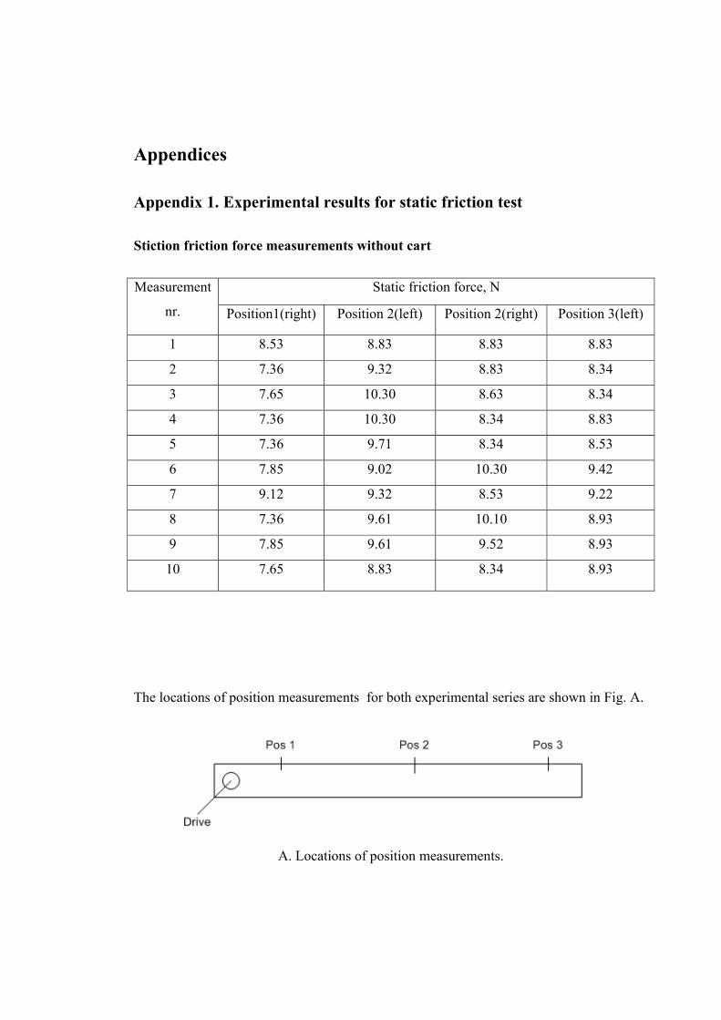
Appendices

Appendix 1. Experimental results for static friction test

Stiction friction force measurements without cart

Static friction force, N Measurement

nr. Position1(right) Position 2(left) Position 2(right) Position 3(left)

1 8.53 8.83 8.83 8.83

2 7.36 9.32 8.83 8.34

3 7.65 10.30 8.63 8.34

4 7.36 10.30 8.34 8.83

5 7.36 9.71 8.34 8.53

6 7.85 9.02 10.30 9.42

7 9.12 9.32 8.53 9.22

8 7.36 9.61 10.10 8.93

9 7.85 9.61 9.52 8.93

10 7.65 8.83 8.34 8.93

The locations of position measurements for both experimental series are shown in Fig. A.

A. Locations of position measurements.

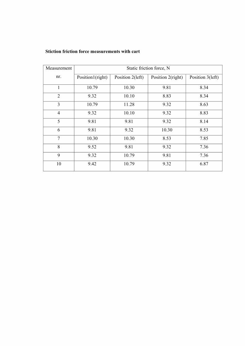
Stiction friction force measurements with cart

Static friction force, N Measurement

nr. Position1(right) Position 2(left) Position 2(right) Position 3(left)

1 10.79 10.30 9.81 8.34

2 9.32 10.10 8.83 8.34

3 10.79 11.28 9.32 8.63

4 9.32 10.10 9.32 8.83

5 9.81 9.81 9.32 8.14

6 9.81 9.32 10.30 8.53

7 10.30 10.30 8.53 7.85

8 9.52 9.81 9.32 7.36

9 9.32 10.79 9.81 7.36

10 9.42 10.79 9.32 6.87

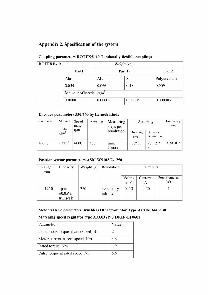
Appendix 2. Specification of the system

Coupling parameters ROTEX®-19 Torsionally flexible couplings

Weight,kg

Part1 Part 1a Part2

Alu Alu S Polyurethane

0.054 0.066 0.18 0.009

Moment of inertia, kgm2

ROTEX®-19

0.00001 0.00002 0.00005 0.000003

Encoder parameters 530/560 by Leine& Linde

Accuracy Parameter Moment of inertia, kgm2

Speed max, rpm

Weight, g Measuring steps per revolution Dividing

error Channel

separation

Frequency range

Value 2.6·10-6 6000 300 max 20000

±50º el 90º±25º el

0..200kHz

Position sensor parameters ASM WS10SG-1250

Outputs Range, mm

Linearity Weight, g Resolution

Voltage, V

Current, A

Potentiometer, kΩ

0…1250 up to ±0.05% full scale

350 essentially infinite

0..10 4..20 1

Motor &Drive parameters Brushless DC servomotor Type ACOM 641.2.30

Matching speed regulator type AXODYN® DKH(-E) 0601

Parameter Value

Continuous torque at zero speed, Nm 2

Motor current at zero speed, Nm 4.6

Rated torque, Nm 1.9

Pulse torque at rated speed, Nm 5.6

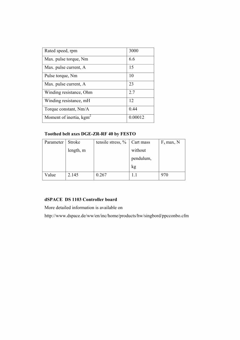
Rated speed, rpm 3000

Max. pulse torque, Nm 6.6

Max. pulse current, A 15

Pulse torque, Nm 10

Max. pulse current, A 23

Winding resistance, Ohm 2.7

Winding resistance, mH 12

Torque constant, Nm/A 0.44

Moment of inertia, kgm2 0.00012

Toothed belt axes DGE-ZR-RF 40 by FESTO

Parameter Stroke

length, m

tensile stress, % Cart mass

without

pendulum,

kg

Fx max, N

Value 2.145 0.267 1.1 970

dSPACE DS 1103 Controller board

More detailed information is available on

http://www.dspace.de/ww/en/inc/home/products/hw/singbord/ppcconbo.cfm

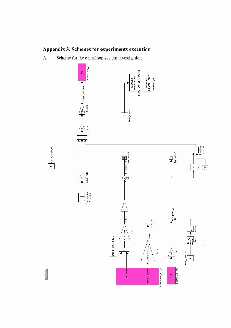
Appendix 3. Schemes for experiments execution A. Scheme for the open-loop system investigation

B. Scheme for PID controller testing

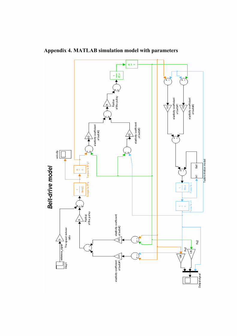
Appendix 4. MATLAB simulation model with parameters

Parameters file % BELT-DRIVE PARAMETERS clear all; r1=0.005; r2=0.02; rho=7000; W=0.02; % the inertia moment of the driving pulley, [kg*m^2] J1=(0.5*pi*rho*W)*(r2^4-r1^4); % the inertia moment of the driven pulley, [kg*m^2] J2 = J1; % the inertia moment of the motor, Jm=0.0012; % the inertia moment of the speed reducer, [kg*m^2] %Jg = 0.1*Jm; % the mass of the cart, [kg] Mc = 1.1; % the speed reducer ratio G = 1; % the radius of the pulleys, [m] R = 0.02; % Belt parameters from manufacturer's data sheet F=970; % [N] epsilon=0.267e-2; %[%] % Belt lenghts [m] at the nominal cart position l3=2.145;

l1=0.74; l2=1.405; % Initial values of belt spring constants % the position dependant elasticity coefficient of the belt 1, [N/m] K1=F/(epsilon*l1); % the position dependant elasticity coefficient of the belt 2, [N/m] K2=F/(epsilon*l2); % the position dependant elasticity coefficient of the belt 3, [N/m] K3=F/(epsilon*l3); %for Tustin's friction model Fk=35; Fv=15; Fs=0; u0=0.019;