Master's Thesis: Modeling and simulation of anaerobic...
144
Modeling and simulation of anaerobic manure digestion into biogas Master’s Thesis in Applied Physics OSKAR DANIELSSON Department of Physics & Engineering Physics Applied Physics Chalmers University of Technology Gothenburg, Sweden 2014 Master’s Thesis 2014:5
Transcript of Master's Thesis: Modeling and simulation of anaerobic...

Modeling and simulation of anaerobicmanure digestion into biogasMaster’s Thesis in Applied Physics
OSKAR DANIELSSON
Department of Physics & Engineering PhysicsApplied PhysicsChalmers University of TechnologyGothenburg, Sweden 2014Master’s Thesis 2014:5


Sammanfattning
I dagens lage ar det allt dyrare att ta hand om godsel fran hastar, men ocksa frandjurparker. Detta projekt, som ar en del i ett storre samarbetsprojekt, syftar till att tafram metoder for att test samrotning mellan djurgodsel och avloppsslam till biogas.
I projektet ar en modell byggd baserad pa Anaerobic digestion model No. 1 (ADM1).Till denna standardmodell har sedan ytterligare ekvationer lagts och flera simuleringarbyggts, med syftet att ta fram verktyg for att undersoka mojligheten till samrotningmellan godsel och slam. Intressanta aspekter sa som optimal blandning och parameter-beroende ar undersokt.
Arbetet ar genomfort i MATLAB, men for att oka nyttan med projektet ar ocksa ettfristaende grafiskt anvandarinterface byggt. Detta later personer utan tillgang till ellerkunskap om MATLAB anvanda den byggda modellen.
Abstract
Today it becomes more and more expensive to take care of produced manure, not onlyfrom horses, but also from zoos. This project, that is a small part of a large collaboration,aims to develop methods to test co digestion of manure and waste water sludge to biogas.
In the project a model based on the Anaerobic Digestion Model No. 1 (ADM1)is built. To this standard model further equations have been added and simulationshave been build, with the aim to develop tools to investigate the possibilities to codigest manure and sludge. Interesting aspects such as optimal mixture and parameterdependence are investigated.
The work is performed in MATLAB, but to make wider use of the project result, astand alone graphical user interface is also created. This lets peoples without knowledgeabout or access to MATLAB use the build model.


Acknowledgements
This Master’s Thesis has been performed at Chalmers University of Technology in col-laboration with SP Energiteknik in Lund. The work has been both fun and interesting.I would like to send many thanks to my main supervisor Magnus Karlsteen at Chalmersthat has taken care of everything from missed spelling, to supporting me in everything.
I will also thank my other supervisor at SP, Karin Willquist, Who has taken her timeto explain every biological and chemical system so that also a physicist can understandthem.
Oskar Danielsson, Gothenburg May 26, 2014


Contents
1 Theory and Resources 11.1 Background . . . . . . . . . . . . . . . . . . . . . . . . . . . . . . . . . . . 11.2 Background . . . . . . . . . . . . . . . . . . . . . . . . . . . . . . . . . . . 2
1.2.1 General . . . . . . . . . . . . . . . . . . . . . . . . . . . . . . . . . 21.2.2 Conditions . . . . . . . . . . . . . . . . . . . . . . . . . . . . . . . 21.2.3 Features . . . . . . . . . . . . . . . . . . . . . . . . . . . . . . . . . 21.2.4 Research questions . . . . . . . . . . . . . . . . . . . . . . . . . . . 31.2.5 Limitations . . . . . . . . . . . . . . . . . . . . . . . . . . . . . . . 31.2.6 Outline . . . . . . . . . . . . . . . . . . . . . . . . . . . . . . . . . 3
2 Theory and Resources 52.1 Abbreviation and things that are good to know . . . . . . . . . . . . . . . 52.2 Units . . . . . . . . . . . . . . . . . . . . . . . . . . . . . . . . . . . . . . . 82.3 Nomenclature . . . . . . . . . . . . . . . . . . . . . . . . . . . . . . . . . . 82.4 Anaerobic Digestion Model No. 1 - ADM1 . . . . . . . . . . . . . . . . . . 8
2.4.1 Basis of the model . . . . . . . . . . . . . . . . . . . . . . . . . . . 82.4.2 Units in ADM1 . . . . . . . . . . . . . . . . . . . . . . . . . . . . . 112.4.3 Nomenclature, Parameters and variables in ADM1 . . . . . . . . . 112.4.4 Dynamic state variables . . . . . . . . . . . . . . . . . . . . . . . . 122.4.5 Biochemical processes . . . . . . . . . . . . . . . . . . . . . . . . . 142.4.6 Physico-chemical processes . . . . . . . . . . . . . . . . . . . . . . 172.4.7 Implementation and regulation of ADM1 . . . . . . . . . . . . . . 17
2.5 Changes made to standard ADM1 . . . . . . . . . . . . . . . . . . . . . . 192.6 Particle Swarm Optimization . . . . . . . . . . . . . . . . . . . . . . . . . 202.7 Horse manure as a resource for biogas production . . . . . . . . . . . . . . 212.8 Waste water sludge as resource for biogas production . . . . . . . . . . . . 212.9 Co-digestion with different substrates . . . . . . . . . . . . . . . . . . . . . 21

CONTENTS
3 Method 223.1 Model implementation . . . . . . . . . . . . . . . . . . . . . . . . . . . . . 22
3.1.1 Model equations . . . . . . . . . . . . . . . . . . . . . . . . . . . . 233.1.2 Verifying the implementation . . . . . . . . . . . . . . . . . . . . . 30
3.2 Simulation . . . . . . . . . . . . . . . . . . . . . . . . . . . . . . . . . . . . 313.2.1 Sensitivity analysis . . . . . . . . . . . . . . . . . . . . . . . . . . . 313.2.2 Variable dependence of parameters . . . . . . . . . . . . . . . . . . 33
3.3 Maximizing gas production . . . . . . . . . . . . . . . . . . . . . . . . . . 333.3.1 PSO implementation . . . . . . . . . . . . . . . . . . . . . . . . . . 34
3.4 GUI . . . . . . . . . . . . . . . . . . . . . . . . . . . . . . . . . . . . . . . 363.4.1 Basins of the GUI . . . . . . . . . . . . . . . . . . . . . . . . . . . 36
4 Results 384.1 Model implementation . . . . . . . . . . . . . . . . . . . . . . . . . . . . . 38
4.1.1 Verifying the implementation . . . . . . . . . . . . . . . . . . . . . 474.1.2 Sensitivity analysis . . . . . . . . . . . . . . . . . . . . . . . . . . . 494.1.3 Variable dependence . . . . . . . . . . . . . . . . . . . . . . . . . . 514.1.4 Maximizing gas production . . . . . . . . . . . . . . . . . . . . . . 514.1.5 GUI . . . . . . . . . . . . . . . . . . . . . . . . . . . . . . . . . . . 52
5 Discussion 565.1 Model implementation . . . . . . . . . . . . . . . . . . . . . . . . . . . . . 565.2 Verifying the implementation . . . . . . . . . . . . . . . . . . . . . . . . . 575.3 Sensitivity analysis . . . . . . . . . . . . . . . . . . . . . . . . . . . . . . . 575.4 Variable dependence . . . . . . . . . . . . . . . . . . . . . . . . . . . . . . 575.5 Maximizing gas production . . . . . . . . . . . . . . . . . . . . . . . . . . 585.6 GUI . . . . . . . . . . . . . . . . . . . . . . . . . . . . . . . . . . . . . . . 595.7 Usability of results . . . . . . . . . . . . . . . . . . . . . . . . . . . . . . . 595.8 Further development . . . . . . . . . . . . . . . . . . . . . . . . . . . . . . 60
5.8.1 Fitting the model to the project . . . . . . . . . . . . . . . . . . . 605.8.2 Building more methods and simulations . . . . . . . . . . . . . . . 60
6 Conclusion 61
Bibliography 62
A Biochemical Rate Matrix 63
B Model parameters 66B.1 Standard ADM1 parameters . . . . . . . . . . . . . . . . . . . . . . . . . . 66B.2 Not standard ADM1 parameters . . . . . . . . . . . . . . . . . . . . . . . 70
C Steady state input variables 71
ii

CONTENTS
D Code 73D.1 Running ADM1 simulations . . . . . . . . . . . . . . . . . . . . . . . . . . 73D.2 ADM1 function file . . . . . . . . . . . . . . . . . . . . . . . . . . . . . . . 76D.3 ADM1 indata file . . . . . . . . . . . . . . . . . . . . . . . . . . . . . . . . 85D.4 Sensitivity analysis . . . . . . . . . . . . . . . . . . . . . . . . . . . . . . . 90D.5 Variable dependence . . . . . . . . . . . . . . . . . . . . . . . . . . . . . . 96D.6 Particle Swarm optimization . . . . . . . . . . . . . . . . . . . . . . . . . . 100D.7 GUI . . . . . . . . . . . . . . . . . . . . . . . . . . . . . . . . . . . . . . . 109
D.7.1 Run GUI (mac) . . . . . . . . . . . . . . . . . . . . . . . . . . . . . 109D.7.2 Run GUI (Windows) . . . . . . . . . . . . . . . . . . . . . . . . . . 110D.7.3 Main GUI . . . . . . . . . . . . . . . . . . . . . . . . . . . . . . . . 112D.7.4 Plot GUI . . . . . . . . . . . . . . . . . . . . . . . . . . . . . . . . 132
iii

1Theory and Resources
1.1 Background
There are exceptionally many horses in Sweden. A lot of those horses are groupedaround cities leading to problems in disposing the manure produced. In those areas ofhigh density of horses there are relative small possibilities in spreading the manure at anown field, due to that the horses are located in or in direct vicinity to the cities and theowners don’t have access to a field for spreading. So the only solution for a lot of horseowning people and organizations are to buy manure disposing services from external.
The horse manure produced during a year in Sweden represents 4.3 TWh [1]. Evenwith this energy potential the cost to get rid of the produced manure is approximately1k SEK per year and horse [2]. A good solution would be to find a use for this energypotential meanwhile the cost for disposing manure in the horse business would decrease.Possibly not to the extent that one gets reimbursement to get rid of the manure, but asfar as one do not need to pay for disposing the manure.
One way of disposing the manure and taking care of the energy potential it containswould be to produce biogas out of the manure. Another solution would be to burn themanure. It is hard to say which one of those methods that is the best. This masterthesis focuses on producing biogas out of the horse manure and further more also onmanure from zoos. The thesis is focused on modeling the digestion process in existingbiogas plants that can be used for testing and verifying what happens when manure isadded to the waste water sludge.
Furthermore, today the society is striving for replacing fossil based energy sources,and here the horse manure can play an important role. By digesting the manure tobiogas the manure can replace part of the fossil raw material used for energy productionin the society today.

1.2. Background 2
1.2 Background
1.2.1 General
The horse business in Vastra Gotalands lan close to Gothenburg started to investigatewhy the costs connected to disposing produced manure were so high. Would it bepossible to do some changes so that they could get rid of the manure without needingto pay for disposing it? They thought about it and started a group effort between alot of different small horse businesses in the region. From this collaboration they foundout that they all had many problems and various solutions. But some of the problemswere not unique, as for example the problem with disposing the manure. The solutionsperhaps were different but the problems were still there.
This master thesis is not directly coupled to the conclusion drawn in the report fromthe small horse businesses [2]. Instead it is part of a large collaboration between Vas-tragotalandsregionen, SP, Boras Energi och Miljo AB, Boras Ridskola, Boras djurparkand Chalmers University of Technology that has as the purpose to find out what to dowith produced manure. Not only by horses, but also from animals at zoos that usuallyalso are situated close to cities. The idea is to compare the pros and cons betweendigesting the manure in existing waste water biogas plants, and burning it to get heatinstead. The idea of the thesis is to simulate the outcome of the digesting in order to beable to say whether a digesting process is preferable or not. The results are then to becompared to results from measurements. The comparison to measurements is not partof the present thesis, but it is done as a part of the collaboration in the larger project.
1.2.2 Conditions
At end of the thesis should the following conditions be fulfilled
• The mathematical anaerobic digestion model no. 1 ADM1 (with small changes)should be used for simulations.
• The robustness of the implemented model should be possible to test.
• The model should be tested on typical data.
• The model should be possible to fit to Gasslosa Avloppsreningsverk in Boras.
• The result of the simulation should be presented in a way so that it could form thebasis for implementation in other biogas plants besides Gasslosa in Boras.
• A software tool that can be used of peoples not experienced with programmingand simulations should be compiled on top of the mathematical model.
1.2.3 Features
Features to include in the solution should be:
1.2. Background 3
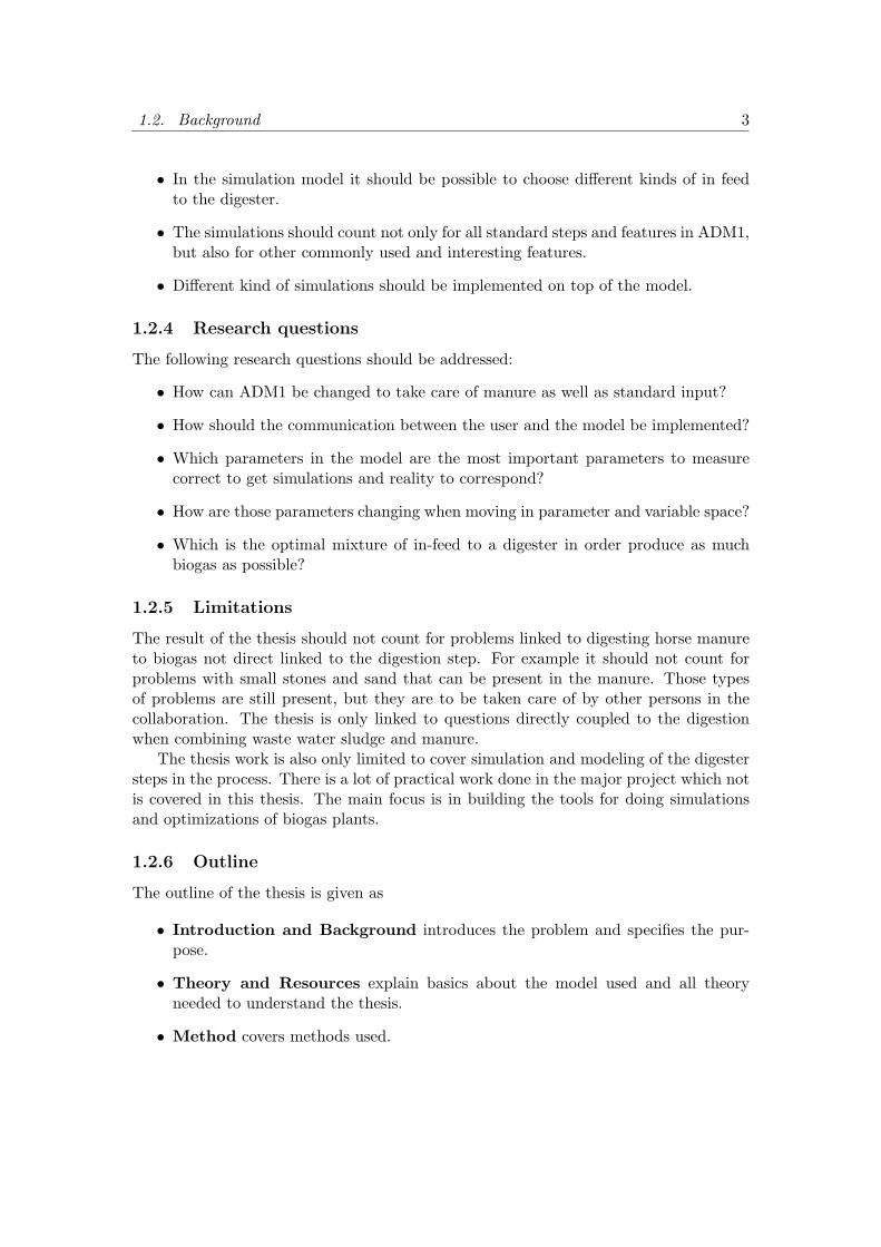
• In the simulation model it should be possible to choose different kinds of in feedto the digester.
• The simulations should count not only for all standard steps and features in ADM1,but also for other commonly used and interesting features.
• Different kind of simulations should be implemented on top of the model.
1.2.4 Research questions
The following research questions should be addressed:
• How can ADM1 be changed to take care of manure as well as standard input?
• How should the communication between the user and the model be implemented?
• Which parameters in the model are the most important parameters to measurecorrect to get simulations and reality to correspond?
• How are those parameters changing when moving in parameter and variable space?
• Which is the optimal mixture of in-feed to a digester in order produce as muchbiogas as possible?
1.2.5 Limitations
The result of the thesis should not count for problems linked to digesting horse manureto biogas not direct linked to the digestion step. For example it should not count forproblems with small stones and sand that can be present in the manure. Those typesof problems are still present, but they are to be taken care of by other persons in thecollaboration. The thesis is only linked to questions directly coupled to the digestionwhen combining waste water sludge and manure.
The thesis work is also only limited to cover simulation and modeling of the digestersteps in the process. There is a lot of practical work done in the major project which notis covered in this thesis. The main focus is in building the tools for doing simulationsand optimizations of biogas plants.
1.2.6 Outline
The outline of the thesis is given as
• Introduction and Background introduces the problem and specifies the pur-pose.
• Theory and Resources explain basics about the model used and all theoryneeded to understand the thesis.
• Method covers methods used.

1.2. Background 4
• Results displays results from modeling and simulations.
• Discussion covers results and explains them.
• Conclusions conclude what is done, and further work possible to do on the model.

2Theory and Resources
2.1 Abbreviation and things that are good to know
This thesis contains several abbreviations and to make it readable those abbreviationscan be found in table 2.1. Due to the fact that the thesis also contains a lot of chemistry,a set of explanations is also included to increase readability for physicists, those can beseen in table 2.2.

2.1. Abbreviation and things that are good to know 6
Table 2.1: Abbreviations
General
Term ExplanationADM1 Anaerobe Digestion Model no. 1COD Chemical Oxygen DemandDAE Differential and Algebraic EquationDE Differential EquationODE Ordinary Differential EquationGUI Graphical User InterfaceThe task group IWA Task Group for Mathematical Modelling of Anaerobic
Digestion Processes - The group who developed ADM1.
Substrates
Term ExplanationLCAF Long Chain Fatty AcidsLCAF – LCAF base equivalentaa Amino acidms Monosaccharidessu Sugarfa Fatty acidva Valeratebu Butyratepro Propionateac Acetateh2 Hydrogench4 MethaneIC Inorganic carbonIN Inorganic nitrogenI Inertsxc Compositesch Carbohydratespr Proteinsli Lipidsc4 Butyrate and Valerate particulatecat Cationsan Anionsva – Valerate acidbu – Butyrate acidpro – Propionate acidac – Acetate acidhco –
3 Bicarbonatenh3 Ammonialac Lactatelac,f Particulate lactate (fermentation)lac,o Particulate lactate (oxidation)ca Calcium

2.1. Abbreviation and things that are good to know 7
Table 2.2: Explanations for physicists
Term Explanation
Acetogenesis A process through which acetate is produced with help ofanaerobic bacterias
Acidogenesis A process where monomers are converted to shorter volatilefatty acids
COD Chemical oxygen demand tells the amount of oxygen neededto decompose a specific amount of organic material. A highCOD value corresponds to a high concentration of organiccompounds in the materials, leading to a high gas exchange.
Extra cellular Outside the cells
Hydrolysis A chemical process where a molecule is divided after wateris added.
Intra cellular Inside the cells
Methanogenesis A biological reaction where acetates are converted intomethane and carbon dioxide
Monod kinetics Mathematical model for growth of microorganisms
Fermentation A metabolic process that converts sugar to acids, gas and/oralcohol
Oxidation Chemical reaction in which a substrate gives away one ormore electrons
Reaction order Determines rate of reactions
β-oxidation Cyclic degradation process of fatty acids in five steps
Arrhenius equation Determines the reaction rates as a function of the tempera-ture
Monomer Unit (molecule) that can be linked to other monomers toform chains
Polymers Large unit consisting of multiple monomers
Inhibition Preventing a chemical reaction
Liquid-liquid process Process only involving liquids
Reactor head space Gas volume of reactor above liquid volume in reactor

2.2. Units 8
2.2 Units
The units in this thesis is chosen to fit the choice of parameters used in ADM1. So forexplanation of the units see section about units in ADM1 2.4.2.
2.3 Nomenclature
The nomenclature of this thesis are chosen to fit the nomenclature of ADM1 for increasedreadability. So for explanation see section about nomenclature in AMD1 2.4.3.
2.4 Anaerobic Digestion Model No. 1 - ADM1
The mathematical anaerobic digestion model ADM1 is the model that the simulations ofthis thesis are based on. The model is developed by IWA Task Group for MathematicalModeling of Anaerobic Digestion Processes [3] and is widely used for modeling of biogasplants. The model consists originally of 29 processes and 24 substances and the substratelevel is of Monod-type kinetics.
The model is changed a bit when implemented in this thesis to fulfill requirementsset up in the project. The difference is not in the main features of the model, but insteadin the amount of substrates in the model. Along with substrates such as sugar, aminoacids and propionate also lactate is added to the process resulting in a more complex,but correct, picture of substrates to take care of. Besides this calcium precipitation isalso added to the model due to its affect on carbon dioxide partial pressure. This sectionfirst covers the standard ADM1 model and then the differences made in this specificimplementation.
In the report written by the IWA task group, here referred to as the task group, themodel is explained [3]. The report explains the different steps and how they are coupledto each other and what affect change in one step will cause in another step. ADM1 isexplained as ”a structured model with disintegration and hydrolysis, acidogenesis, aceto-genesis and methanogenesis steps”.
ADM1 is created to be used with a lot of possible types of anaerobic processes andmight therefore not be as exact as other models that are developed for a specific task. Theadvantage of this is however that the model can be applied to a wide field of applications.
2.4.1 Basis of the model
The model models cellular kinetics as substrate uptake, growth and decay. Of which thesubstrate uptake (for different substrates) can be described with the formula
vi = kmSi
Si +KsXi × Ii (2.1)
Where vi is the actual uptake, km is the maximum uptake rate, SiSi+Ks
is the substrateconcentration factor, Xi is the biomass concentration and Ii is the inhibition factor,

2.4. Anaerobic Digestion Model No. 1 - ADM1 9
explained below. The reactions taking place can be seen in the ADM1 report’s matrixfor biochemical reactions, which can be found in table A.1 and A.2 in appendix A. Thisis the normal way of presenting the biochemical equations in the model, but due to thefact that this thesis belongs to the physics field, all reactions are also presented as normalsets of differential equations in the method section, see section 3.
Disintegration is mainly included into the model to describe degradation of com-posite materials to well known inerts, particulate carbohydrates, proteins and lipids.The second step is enzymatic reactions that convert particulate carbohydrates, lipidsand proteins to monosaccharides (MS), amino acids (AA) and long chain fatty acidsrespectively (LCAF).
The model contains both biochemical and physico-chemical reactions, of which thephysico-chemical reactions are implemented as reversible, while the biochemical reac-tions are implemented as irreversible reactions. The biochemical processes are normallycatalyzed by intra- and extracellular enzymes that acts on the available biomass, whilethe physico-chemical processes not are biological mediating. Physiochemical processesinclude ion association/dissociation and gas-liquid transfer.
The flow of the material in the model can be seen as the flow of COD in the model.The flow rates and the different steps can therefore be visualized as a COD-flow chart,which can be seen in figure 2.1. The picture comes from [3]. In order to fit the model toa specific type of mixture or process a lot of things can be done before the first step inthe model. For example the mixture between sludge and manure can be changed. Theinflow to this block will define how much manure and how much standard waste waterthat are in the inflow to the digestion chamber.
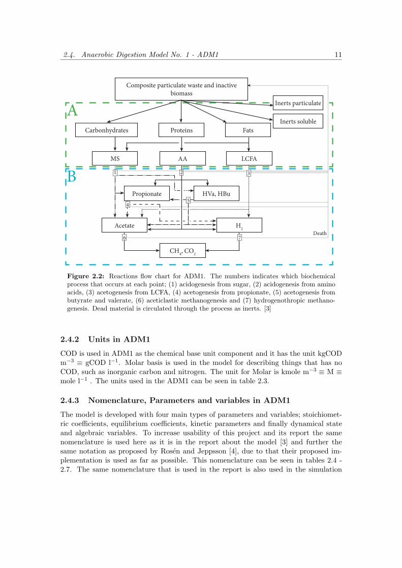
If the main interest not is in finding a quick way to see all flows in the model, butinstead in all reactions that is taking place in the modeled process, the flowchart infigure 2.2 can be seen. The figure can be divided into two parts, where the top partmarked with ”A” takes care of the hydrolysis of substrate and the second part, denoted”B”, handle the reactions catalyzed by different groups of Monod type kinetics. In thesecond part different numbers are presented describing which biochemical reaction thatoccurs in each point.

2.4. Anaerobic Digestion Model No. 1 - ADM1 10
Input Material (100%)
Inerts 10%
Lipids 30%Proteins 30%Carbonhydrates 30%
MS 10% AA 30% LCFA 29%
HPr, HBu, HVa 29%
Acetic 64% H2 26 %
CH4 90%
Manure X% Wastewater (100-X)%
Figure 2.1: Flow chart for COD ind ADM1. The figure comes from the report aboutADM1 [3]. This flow model is modified a bit to fit the implementation done in this work,see section 2.5 for further explanation.
2.4. Anaerobic Digestion Model No. 1 - ADM1 11
A
B
Composite particulate waste and inactive biomass
Inerts particulate
FatsProteinsCarbonhydrates
MS AA LCFA
Inerts soluble
Propionate HVa, HBu
Acetate H2
CH4, CO
2
Death
1 2 3
45
6 7
Figure 2.2: Reactions flow chart for ADM1. The numbers indicates which biochemicalprocess that occurs at each point; (1) acidogenesis from sugar, (2) acidogenesis from aminoacids, (3) acetogenesis from LCFA, (4) acetogenesis from propionate, (5) acetogenesis frombutyrate and valerate, (6) aceticlastic methanogenesis and (7) hydrogenothropic methano-genesis. Dead material is circulated through the process as inerts. [3]
2.4.2 Units in ADM1
COD is used in ADM1 as the chemical base unit component and it has the unit kgCODm−3 ≡ gCOD l−1. Molar basis is used in the model for describing things that has noCOD, such as inorganic carbon and nitrogen. The unit for Molar is kmole m−3 ≡ M ≡mole l−1 . The units used in the ADM1 can be seen in table 2.3.
2.4.3 Nomenclature, Parameters and variables in ADM1
The model is developed with four main types of parameters and variables; stoichiomet-ric coefficients, equilibrium coefficients, kinetic parameters and finally dynamical stateand algebraic variables. To increase usability of this project and its report the samenomenclature is used here as it is in the report about the model [3] and further thesame notation as proposed by Rosen and Jeppsson [4], due to that their proposed im-plementation is used as far as possible. This nomenclature can be seen in tables 2.4 -2.7. The same nomenclature that is used in the report is also used in the simulation

2.4. Anaerobic Digestion Model No. 1 - ADM1 12
Table 2.3: Units to be used in the ADM1 model
Measurement Units
Concentration kgCOD m−3
Concentration (non-COD) kmoleC m−3
Concentration (nitrogen non-COD) kmoleN m−3
Pressure bar
Temperature K
Distance m
Volume m3
Energy J (kJ)
Time d (day)
Table 2.4: Stoichiometric coefficients [3]
Symbol Description Units
Ci Carbon content of component i kmoleC kgCOD – 1
Ni Nitrogen content of component i kmoleN kgCOD – 1
νi,j Rate coefficient for component i on process j nominally kgCOD – 1
fproduct,substrate Yield (catabolism only) of product on substrate kgCOD kgCOD – 1
implementation.
2.4.4 Dynamic state variables
The model can be implemented as a set of differential equations (DE) or as a set ofDifferential and Algebraic Equations (DAE), of which the DE method is used.

2.4. Anaerobic Digestion Model No. 1 - ADM1 13
Table 2.5: Equilibrium coefficients and constants [3]
Symbol Description Units
Hgas Gas law constant (equal to K – 1H ) bar M – 1 (bar m 3 kmole – 1)
Ka,acid Acid-base equilibrium coefficient M (kmole m – 3)
KH Henry’s law coefficient M bar – 1 (kmole m – 3bar – 1)
pKa log10[Ka]
R Gas law constant (8.314× 10⁻²) bar M – 1K – 1 (bar m 3kmole – 1K – 1
∆G Free energy J mole – 1
Table 2.6: Kinetic parameters and rates [3]
Symbol Description Units
kA/Bi Acid base kinetic parameter M – 1d – 1
kdec First order decay rate d – 1
Iinhibitor,process Inhibition function (see Kl)
kprocess First order parameter (normally for d – 1
hydrolysis)
kLa Gas-liquid transfer coefficient d – 1
kl, inhibit, substrate 50% inhibitory concentration kgCODm – 3
km, process Monod maximum specific uptake rate kgCOD S kgCOD X – 1 d – 1
(µmax/Y)
kS, process Half saturation value kgCOD S m – 3
ρj Kinetic rate of process j kgCOD S m – 3d – 1
Ysubstrate Yield of biomass on substrate kgCOD X kgCOD – 1S
µmax Monod maximum specific growth rate d – 1

2.4. Anaerobic Digestion Model No. 1 - ADM1 14
Table 2.7: Dynamic state and algebraic variables [3]
Symbol Description Units
pH − log10[H+]
pgas,i pressure of gas i bar
Pgas Total gas pressure bar
Si Soluble component i kgCOD m – 3
tres, X Extended retention of solids d
T Temperature K
V Volume m 3
Xi Particulate component i kgCOD m – 3
2.4.5 Biochemical processes
The model includes three main biological cellular steps; acidogenesis, acetogenesis andmethanogenesis, as well as an extracellular disintegration step.
The disintegration step is supposed to contain several steps so that the product fromthe step can be assumed to be homogeneous before it disintegrates to carbohydrates,proteins and lipids, reason for that is that multiple digestion ensures total digestion.Those can then in the next step be disintegrated in the next biochemical steps. [3]
In the report written by the IWA task group the key rate equation in the ADM1 isthe substrate uptake, which is based on substrate level Monod-type kinetics.
To know how to implement the biochemical steps the rate equation matrices should bestudied A.1 and A.2. This matrix includes booth the rates for the equations implementedin the model. The matrices can be seen in Appendix A. To get a more common way ofseeing this for a physicist the equations in section 3.1.1 are presented, which presentsthe matrices’ reactions as normal ODE system.
Disintegration and hydrolysisDisintegration and hydrolysis are extra-cellular steps handling breakdown and solubi-lization of complex organic materials to monomers. Those substrates are composite par-ticulates and particulate carbohydrates, proteins and lipids. Of which carbohydrates,proteins and lipids can be digested to monosaccharides, amino acids and long chain fattyacids with help of enzymatic reactions.
A mainly non-biological disintegration step is included as a first step in the modelto make the model possible to use for a large variety of input materials. The enzymaticstep is a complex combination of multiple steps taking care of carbohydrates, proteinsand lipids. Due to that first order and second order kinetics could fit biogas productionequally well, the task group did find out that it was enough to use a more easy to use

2.4. Anaerobic Digestion Model No. 1 - ADM1 15
model with only first order kinetics. [3]
AcidogenesisAcidogenesis, or fermentation is generally defined as an anaerobic acid-producing micro-bial process without an additional electron acceptor or donor. The IWA task group hasdecided to use glucose molecule as modeling monomer for the process. Furthermore, thetask group decided to include acetate, propionate and butyrate in the model due to itsimportance as end-products from the digestion of monosaccharides acidogenesis.
Syntrophic hydrogen-producing acetogenesis and hydrogen-utilizing methano-genesisDegradation of organic acids to acetate is an oxidation process without internal electronacceptors and therefore is the process depending on external acceptors such as hydrogenions or carbon dioxide to produce hydrogen gas. The thermodynamics of syntrophicreaction described here is only possible in a narrow range of hydrogen concentration.According to the IWA task group this is important for modeling, due to its affect forhydrogen inhibition, half saturation coefficients and yields, and it is therefore includedin ADM1. [3]
The electron carrier described here can not only be hydrogen, but also formate.However due to the task group has decided to only count on hydrogen as electron carrier,formate is not taken care of in this text.
The anaerobic degradation of fatty acids above propionate is done by the so calledβ-oxidation which is a cyclic process. The substrates produced from this degradationtaken care of in the ADM1 are butyrate, valerate and LCFA.
To model hydrogen inhibition for acetogenesis is the more simple non-competitiveinhibition used in the model and liquid phase hydrogen concentration is used for hydrogeninhibition.
Aceticlastic methanogenesisThe most important step in forming methane from acetate contains cleaving of acetateto methane and carbon dioxide.
CH3COOH −−→ CH4 + CO2 (2.2)
InhibitionInhibition is included in ADM1 in form of Biostatic inhibition, which is a ”Nonreactivetoxicity, normally reversible” form of inhibition affecting kinetic uptake and growth [3].
The affect of included inhibition in the models rate equations is calculated on theform
ρj =kmSK+
s SX · I1 · I2 · · · In (2.3)

2.4. Anaerobic Digestion Model No. 1 - ADM1 16
Table 2.8: Forms of inhibition used in ADM1. Forms not used but mentioned in the taskgroups report are skipped to mention here. [3]
Description Equation Used for
Non-competitive inhibi-tion
I = 11+S1/K1
Free ammonia and hy-drogen inhibition
Empirical upper andlower inhibition
I = 1+2×100.5(pH
LL−pH
UL)
1+10(pH−pH
UL)+10
(pHLL−pH) pH inhibition when
both high and low pHinhibition occurs
Empirical lower inhibi-tion only
I = exp
(−3(
pH−pHLLpHUL−pHLL
)2) ∣∣∣∣∣
pH<pHUL
I = 1∣∣pH>pHUL
pH inhibition when onlylow pH inhibition oc-curs
Competitive uptake I = 11+S1/S
Butyrate and valeratecompetition for C4
Secondary substrate I = 11+K1/S1
All uptake, to inhibituptake when CIN ∼ 0
Where the first part of the function is the uninhibited Monod-type uptake andI1...n−−f(SI,1...n) are the inhibited functions presented in the biochemical rate matrices
A.1 and A.2. For those cases where this equation not can be used are instead theinhibition functions presented in table 2.8.
pH inhibition are used for all intracellular interactions in ADM1.
Temperature dependenceFor anaerobic digesting processes there are three major temperature ranges one usuallytalks about. Those are psychrophilic (4-15°C), mesophilic (20-40°C) and thermophilic(45-70°C).
According to the task group there are three major system types that need to bemodeled with respect to temperature.
1. Temperature controlled with small changes in operating temperature (±3°C).
2. Uncontrolled but fluctuating within one range (either mesophilic or thermophilic).
3. Fluctuation between mesophilic and thermophilic temperatures.
The temperature dependence follows Arrhenius equation to an optimal temperatureand then drops rapidly to zero. Although this implements that there are a continuousfunction describing temperature dependence are separate values used for thermophilicand mesophilic conditions in ADM1. [3]

2.4. Anaerobic Digestion Model No. 1 - ADM1 17
2.4.6 Physico-chemical processes
Physico-chemical processes are processes that not are biological mediating processes.Those include liquid-liquid processes, liquid-gas processes and liquid-solid processes. InADM1 the last type of mentioned processes are excluded, but in this implementationcalcium carbonate precipitation are added to model affects of carbon dioxide production.When modeling a system physico-chemical processes are really important due to theirkey role, which for example includes parameters such as pH and gas flow.
Liquid-liquid processesThe liquid-liquid processes that are modeled mainly take care about ion association anddissociation with hydrogen and hydroxide ions. Due to the rapidness of association/dis-sociation processes those processes are often referred to as equilibrium processes.
Liquid-gas processesWhen creating the model, the task group considered the following three gas componentsimportant H2, CH4 and CO2 due to their strong effect on biological processes or outputsof them and included them into the model.
The gas and liquid phases will, when they are in contact to each other reach anequilibrium state [3]. When the gas phase are enough diluted Henry’s law can be usedto describe the concentrations
KHpgas,i,ss − Sliq,i,ss = 0 (2.4)
Where Sliq,i,ss is the steady state liquid phase concentration for component i, pgas,i,ss
is the steady state gas phase partial pressure of component i and KH is Henry’s lawcoefficient.
Temperature dependencePhysico-chemical systems are highly affected by change in temperature, due to changesin equilibrium coefficients.
2.4.7 Implementation and regulation of ADM1
The model can be implemented in two main different ways; firstly a set of differentialequations (DE) can be used and secondly a set of algebraic differential equations (DAE)can be used, the implementation approach used is the DE method, implying that thisreport only covers this method.
Liquid phase equationsThe reaction system is implemented as a system of mass balance reactions, those massbalance reactions can be written as

2.4. Anaerobic Digestion Model No. 1 - ADM1 18
dVSliq,i
dt= qinSin,i − qoutSliq,i + V
19∑j=1
ρjνi,j (2.5)
Where∑19
j=1 ρjνi,j is the sum of specific kinetic rates for process j multiplied by νi,j,which is the rate coefficient pof component i on process j. This includes shift in volume,but if a constant volume and flow is assumed, (q−−qin
−−qout) can be used implementingthat the reaction boils down to.
dSliq,i
dt=
qSin,i
Vliq
−qSliq,i
Vliq
+19∑j=1
ρjνi,j (2.6)
In addition to the rate equations specified the biochemical rate matrices (A.1) and(A.2) do also the following rate equations need to be added to the simulation
ρT,H2= kLa (Sliq,H2
−16 KH,H2pgas,H2
)
ρT,CH4= kLa (Sliq,CH4
−64 KH,CH4pgas,CH4
)
ρT,IC = kLa (Sliq,CO2−KH,CO2
pgas,CO2)
(2.7)
Where ρT,i is the transfer rate of gas i and Sliq,CO2is the fraction of inorganic carbon
as CO2.Besides this also ion equations needs to be added to the simulation, reaction rates
for those looks like:
ρA,i = kA,B,i · (Si− · (Ka,i + Sh+)−Ka,i · Si) (2.8)
Where i stands for ion number i, Ka i is the acid-base equilibrium coefficient for acidi, Sh+ is the concentration of H+ ions and kA,B,i is the acid base kinetic parameterparameter for acid i. From those rates DE equations looks like
dSi−dt
= −ρA,i (2.9)
Gas phase equationsThe gas phase rate equations are very similar to the liquid phase equations, except thereis no advective influent flow [3]. For a system with constant gas volume the equationslooks like
dSgas,i
dt= −
Sgas,iqgas
Vliq
+ ρT,i
Vliq
Vgas(2.10)
The factorVliq
Vgasis required due to that gas transfer kinetics is liquid-volume specific.
2.5. Changes made to standard ADM1 19
The pressure of each gas can be calculated with help of the gas law and the factors(16, 64, 1 ) introduced in equation (2.7) according to [3]. The factors comes correspondsto COD equivalents of the gases.
pgas,H2= Sgas,H2
RT/16
pgas,CH4= Sgas,CH4
RT/64
pgas,CO2= Sgas,CO2
RT
(2.11)
According to the task group it is accurate to assume that the reactor headspace issaturated with water vapor. By using the formula for gas pressure and inserting valuesfor water vapor in it one will obtain values for the water vapor pressure. From this canthe total gas flow be calculated, by setting it equal to the total gas transfer, correctedfor the water vapor
qgas =RT
pgas−pgas,H2O
Vliq
(ρT,H2
16+ρT,CH4
64+ ρT,CO2
)(2.12)
RegulationWhen implementing the model, a lot of different equations and variables are to beused. The coupling between those variables is large and by changing in one part of thesystem one other part of the system might be affected. For example by acceleratingthe production in one part of the system might inhibit an other part of the systemthen leading to for example decreased digesting or gas production in a third part of thesystem.
2.5 Changes made to standard ADM1
The model implemented in this thesis is not exactly the same as the standard ADM1described by [3]. Instead new equations proposed by Willquist et al. [5] are added.Those equations follows the same logic as the other reactions, but ad extra possibilitiesto simulate the process in the biogas plant.
To the substrates are lactates added in terms of fermentation and oxidation. Reasonfor adding them both is that it could be interesting in some applications to see whathappens with different types of lactate biomass. The equations derived from lactate canbe seen in the same biochemical rate matrix as all other biochemical processes A.1 andA.2.
Besides lactate, also precipitation of calcium is added to the model. Due to thatprecipitation are affecting the production of carbon dioxide, which highly affects theoverall production of biogas, it is interesting to have the possibility to correct for thoseaffects during simulation of an entire system. This precipitation is a liquid-solid process,which was neglected by the task group.

2.6. Particle Swarm Optimization 20
2.6 Particle Swarm Optimization
Particle Swarm Optimization (PSO) is a biologically inspired optimization method thatmimics the advantage of forming swarms. In nature the tendency of forming swarmsappears in many different spices. For example the tendency can be found in populationsof fishes and birds. The advantages of forming swarms are for example the protectionfrom predators. An individual close to the center of the swarm is unlikely to be attackedby a predator and the swarm may confuse the predator by coordinated movements, butmore important is that the risk for each individual to be hit by a predator decreasesrapidly in a large swarm. However if the predator has located the swarm he do knowwhere the pray is, so the likelihood for that any of the prays will be hit is quite large.[6]
A swarm consisting of a lot of individuals has a large advantage in searching forthings, for example food, due to the large amount of individuals contributing to thesearch. By coordinating the swarm the search can be even more effective and this iswhat particle swarm optimization method is about.
PSO-algorithm tries to capture the beneficial properties of a swarm. Aspects mim-icked are those who in an optimization point of view are important, namely the searchefficiency of a swarm. In PSO a population of possible solutions to an optimizationproblem is founded and evaluated. The initialization of those solutions are randomlychosen inside an allowed search space. The best known position in search space for allsolutions is saved as the best know global solution and the best known (at initializationthe only known) solution for each particle is saved as the local best known solution sofar.
By steering all test solutions in direction of the global best known position morepositions in search space are evaluated in a more efficient manner, compared to randomsearch. There are however some drawbacks with this method, no guaranties that thebest solution is ever found can be given. The advantages of using PSO are however inthe amount of parameters that can be evaluated and the amount of information neededabout the optimization system needed. The complexity of the ADM1 system togetherwith the large amount of parameters makes the use of PSO a good choice.

2.7. Horse manure as a resource for biogas production 21
2.7 Horse manure as a resource for biogas production
This project aims to find a good way of mixing horse manure with waste water as aresource for a biogas plant. Horse manure is not only hard to get rid of, it is also a goodresource to more carbon in the biogas processes. When adding horse manure to the rawmaterial in biogas processes do one not only get manure, one do also get a lot of beddingmaterial included in the manure waste, leading to low biogas yield per volume unit ofraw material. However horse manure has, as stated, a lot of carbon that can be used inthe process to balance the carbon/nitrogen ratio. [7]
Dry weight of horse manure/bedding mixture is approximately 20-25% of whichabout 75% are organic materials interesting for biogas production. Mixtures will varydepending on bedding materials, feed, size of horse and activity of the horse. [7]
2.8 Waste water sludge as resource for biogas production
Sludge for biogas production is characterized by the fact that it has been digested inearlier steps of some purification process and therefore it contains a lower amount ofmaterial that can be digested to manufacturer biogas. The dry weight for sludge variesbetween 2-100%. [7]
2.9 Co-digestion with different substrates
Normally when one talks about co-digestion of different substrates, one mean that amain substrate is used and to this a secondary substrate is added in smaller amounts.
The co-digestion branch of digestion to biogas is interesting due to the possibilitiesin trimming the process in the direction wanted. Processes can be both more stable andmore effective when a co-digestion method is applied, as the full effect of the digestionchamber is used. For example, a bad carbon/nitrogen ratio can be improved with dif-ferent mixtures of substrates. Furthermore manure could be digested in existing plantswithout needs for enormous investments in new plants.

3Method
The main part of the work done in this thesis is in implementing ADM1, testing andverifying the model and finally compile results from the simulations to something thatcan be used for co digesting manure with waste water sludge.
3.1 Model implementation
When implementing the model one report by Rosen and Jeppsson [4] have been used,that deals with ADM1 implementation through an ODE system as well as a DAE system,of which the ODE implementation is used in this work. In the report it is discussed thatthe initial carbon and nitrogen balance when digesting composites to carbohydrates,proteins and lipids not holds. In the report do Rosen and Jeppsson discuss why thebalance not holds and what needed to be changed for it to hold. The affect of theoriginal incomplete balances is that in the first step of the model it disappears about 5-6% of carbon and nitrogen, but by changing the fraction of obtained proteins, lipids andcarbohydrates from the initial composites are the carbon and nitrogen balances closed.
In this thesis implementation of ADM1 is therefore the changes proposed by Rosenand Jeppsson done in order to close the carbon and nitrogen balances.
The variable names in this thesis are also consistent with the one used by Rosenand Jeppsson in order to increase readability of the implementation. The structure doesalso follow the one in the report due to readability and to make it easier for furtherimplementations of the model.
However does the implementation not completely follow the implementation proposedby Rosen and Jeppsson due to that new equations are added to the model in order totake care of other, not standard ADM1, substrates. Those equations are proposed byWillquist et al. [5]. The new equations take care of lactate and calcium. Reason foradding those equations is that one of the main part of this project, SP Energiteknikin Lund, is interested in those two substrates and how they affects the outcome of the

3.1. Model implementation 23
simulations. However are those equations not included in the theoretical testing of thiswork due to that those equations not are standard equations and therefore it is notpossible to verify the effect of those equations. This does not mean that the equationsnot are tested, they are not only included inside the testing and verifying presented here.
Lactate uptake is implemented in form of oxidation and fermentation processes. De-cay of lactate biomass is also implemented separately for fermentation and oxidation.Calcium is implemented as precipitation in the model.
The model is built in a way so that if one not have some of the substrates presentedin the model, this can be set to zero and Willquist therefore not affect the simulationoutcome. For example, if one is interested in standard ADM1 without lactate andcalcium those two substrates can be set to zero and will then not affect outcome of themodel, hence the standard ADM1 implementation without lactate and calcium can beobtained, by setting lactate and calcium amounts to zero.
3.1.1 Model equations
In order to describe the model implemented it is important to know all the equationsimplemented in the system. The most of the equations can in a quick way be seen in thebiochemical rate matrices A.1-A.2. However to get a complete overview of the systemimplemented are here all equations described in a standard way for a physicist.
The equations are built up by all the reactions occurring in the system. However thereare a lot of parameters as well as variables. All of those parameters define the positionin parameter space at which the reactions take place in. Some of those parameters canbe modified to fit an implemented process, meanwhile some of them are fixed due tolaws of nature. All of those parameters can be found in appendix B.
Process ratesBiochemical process rates for standard ADM1 (line 1-19) and new process rates (line20-23).

3.1. Model implementation 24
ρ1 = kdis ·Xc
ρ2 = khyd,ch ·Xch
ρ3 = khyd,pr ·Xpr
ρ4 = khyd,li ·Xli
ρ5 = km,su ·Ssu
KS,su + Ssu·Xsu · I5
ρ6 = km,aa ·Saa
KS,aa + Saa·Xaa · I6
ρ7 = km,fa ·Sfa
KS,fa + Sfa·Xfa · I7
ρ8 = km,c4 ·Sva
KS,c4 + Sva·Xc4 ·
svaSbu + Sva + 1e−6
· I8
ρ9 = km,c4 ·Sbu
KS,c4 + Sbu·Xc4 ·
sbuSva + Sbu + 1e−6
· I9
ρ10 = km,pro ·Spro
KS,pro + Spro·Xpro · I10
ρ11 = km,ac ·Sac
KS,ac + Sac·Xac · I11
ρ12 = km,h2 ·Sh2
KS,h2 + Sh2·Xh2 · I12
ρ13 = kdec,Xsu ·Xsu
ρ14 = kdec,Xaa ·Xaa
ρ15 = kdec,Xfa ·Xfa
ρ16 = kdec,Xc4 ·Xc4
ρ17 = kdec,Xpro ·Xpro
ρ18 = kdec,Xac ·Xac
ρ19 = kdec,Xh2 ·Xh2
ρ20 = km,lacf ·Slac
KS,lacf + Slac·Xlacf · I20
ρ21 = km,laco ·Slac
KS,laco + Slac·Xlaco · I21
ρ22 = kdec,Xlacf ·Xlacf
ρ23 = kdec,Xlaco ·Xlaco
(3.1)
To compensate for bad choices of Sbu and Sva a small constant had been added toexpressions ρ8 and ρ9, according to [4].

3.1. Model implementation 25
Acid-base rates
ρA,4 = kA,Bva(Sva−(Ka,va + SH+)−Ka,vaSva)ρA,5 = kA,Bbu(Sbu−(Ka,bu + SH+)−Ka,buSbu)ρA,6 = kA,Bpro(Spro−(Ka,pro + SH+)−Ka,proSpro)ρA,7 = kA,Bac(Sac−(Ka,ac + SH+)−Ka,acSac)ρA,10 = kA,Bco2(Shco3−(Ka,co2 + SH+)−Ka,co2SIC)ρA,11 = kA,BIN (Snh3(Ka,IN + SH+)−Ka,INSIN )
(3.2)
Gas transfer rates
ρT,8 = kLa(Sh2 − 16 ·KHH ,h2pgas,h2)ρT,9 = kLa(Sch4 − 64 ·KHH ,ch4pgas,ch4)ρT,10 = kLa(Sco2 −KHH ,co2pgas,co2)
(3.3)
Precipitation ratesThis equation are new compared to standard ADM1.
ρP,24 =
0 : Sca, Shco3− < 0
Kr,caco3 ·(√
Sca · Shco3− −KS,p,caco3
)2: Sca, Shco3− ≥ 0
(3.4)
Process inhibitionpH = − log10(SH+) (3.5)
IpH,aa =
exp
(−3(
pH−pHUL,aapHUL,aa−pHLL,aa
)2)
: pH < pHUL,aa
1 : pH > pHUL,aa
IpH,ac =
exp
(−3(
pH−pHUL,acpHUL,ac−pHLL,ac
)2)
: pH < pHUL,ac
1 : pH > pHUL,ac
IpH,h2 =
exp
(−3(
pH−pHUL,h2
pHUL,h2−pHLL,h2
)2)
: pH < pHUL,h2
1 : pH > pHUL,h2
(3.6)
In the report by Rosen and Jeppsson [4] it is discussed about IpH,i functions above,that are original from the standard ADM1 model [3]. Rosen and Jeppsson proposessome other functions that can be used if there are problems with stability of thoseswitch functions. In our implementation were this not a problem and therefore were thestandard model for pH inhibition used.

3.1. Model implementation 26
IIN,lim =1
1 +KS,IN/SIN
Ih2,fa =1
1 + Sh2/KI,h2,fa
Ih2,c4 =1
1 + Sh2/KI,h2,c4
Ih2,pro =1
1 + Sh2/KI,h2,pro
Inh3 =1
1 + Snh3/KI,nh3
I5,6 = IpH,aa · IIN,limI7 = IpH,aa · IIN,lim · Ih2,fa
I8,9 = IpH,aa · IIN,lim · Ih2,c4
I10 = IpH,aa · IIN,lim · Ih2,pro
I11 = IpH,aa · IIN,lim · Inh3
I12 = IpH,h2 · IIN,lim
Ih2,laco =1
1 + Sh2/KI,h2,laco
I20 = IIN,lim
I21 = Ih2,laco · IIN,lim
(3.7)
Soluble phase equationThe nomenclature here follows Rosen and Jeppssons nomenclature [4]. The idea ofdividing the equations into sections comes from their report. The reason for keeping thesame dividing here is to make it more readable and comparable.
Differential equations 1-4 for soluble matter
StatedSsu
dt = qinVliq
(Ssu,in − Ssu) + ρ2 + (1− ffali) ρ4 − ρ5 [1]
dSaadt = qin
Vliq(Saa,in − Saa) + ρ3 − ρ6 [2]
dSfadt = qin
Vliq(Sfa,in − Sfa) + ffa,liρ4 − ρ7 [3]
dSvadt = qin
Vliq(Sva,in − Sva) + (a− Yaa) fva,aaρ6 − ρ8 [4]
Differential equations 5-8 for soluble matter. Equation 6-8 are modified to count forlactate.

3.1. Model implementation 27
StatedSbu
dt = qinVliq
(Sbu,in − Sbu) + (1− Ysu) fbu,suρ5 + (1− Yaa) fbu,aaρ6 − ρ9 [5]dSpro
dt = qinVliq
(Spro,in − Spro) + (1− Ysu) fpro,suρ5 + (1− Yaa) fpro,aaρ6 + (1− Yc4)0.54ρ8 − ρ10
(1− Ylacf )0.785ρ20 [6]
dSacdt = qin
Vliq(Sac,in − Sac) + (1− Ysu) fac,suρ5 + (1− Yaa) fac,aaρ6 + (1− Yfa)0.7ρ7+
(1− Yc4)0.31ρ8 + (1− Yc4)0.8ρ9 + (1− Ypro)0.57ρ10 − ρ11
(1− Ylacf )0.215ρ20 + (1− Ylaco)23ρ21 [7]
dSh2dt = qin
Vliq(Sh2,in − Sh2) + (1− Ysu)fh2.suρ5 + (1− Yaa)fh2,aaρ6 + (1− Yfa)0.3ρ7+
(1− Yc4)0.15ρ8 + (1− Yc4)0.2ρ9 + (1− Ypro)0.43ρ10 − ρ12 − ρT,8 + (1− Ylaco)13ρ21 [8]
Differential equations 9-12 for soluble matter. Equations 10 and 11 are modified tocount for lactate.
StatedSch4
dt = qinVliq
(Sch4,in − Sch4) + (1− Yac)ρ11 + (1− Yh2)ρ12 − ρT,9 [9]
dSIC∗
dt = qinVliq
(SIC,in − SIC)−23∑j=1
( ∑i=1−9,11−24,36−38
Ciνi,jρj
)[10]
dSINdt = qin
Vliq(SIN,in − SIN )− YsuNbacρ5 + (Naa − YaaNbac)ρ6YfaNbacρ7 − YfaNbacρ8−
Yc4Nbacρ9 − YproNbacρ10 − YacNbacρ11 − Yh2Nbacρ12 − YlacfNbacρ20 − YlacoNbacρ21
+(Nbac −Nxc)∑
i=13−19,22−23
ρi + (Nxc − fxI,xcNI − fsI,xcNI − fpr,xcNaa)ρ1 [11]
dSIdt = qin
Vliq(SI,in − SI) + fsI,xcρ1 [12]
∗ See equation (3.8) for explanation.The sum in the equation for the tenth state is calculated as
19∑j=1
∑
i=1−9,11−24,36−38
Ciνi,jρj
=∑
k=1−12,20−21
skρk+s13(ρ13+ρ14+ρ15+ρ16+ρ17+ρ18+ρ19+ρ22+ρ23)
(3.8)

3.1. Model implementation 28
where
s1 = −Cxc + fsI,xcCsI + fch,xcCch + fpr,xcCpr + fli,xcCli + fxI,xcCxI
s2 = −Cch + Csu
s3 = −Cpr + Caa
s4 = −Cli + (1− ffa,li)Csu + ffa,liCfa
s5 = −Csu + (1− Ysu)(fbu,suCbu + fpro,suCpro + fac,suCac) + YsuCbac
s6 = −Caa + (1− Yaa)(fva,aaCva + fbu,aaCbu + fpro,aaCpro + fac,aaCac) + YaaCbac
s7 = −Cfa + (1− Yfa)0.7Cac + Yc4Cbac
s8 = −Cva + (1− Yc4)0.54Cpro + (1− Yc4)0.31Cac + Yc4Cbac
s9 = −Cbu + (1− Yc4)0.8Cac + Yc4Cbac
s10 = −Cpro + (1− Ypro)0.57Cac + YproCbac
s11 = −Cac + (1− Yac)Cch4 + YacCbac
s12 = −Ch2 + (1− Yh2)Cch4 + Yh2Cbac
s13 = −Cbac + Cxc
s20 = −Clac + (1− Ylacf )0.785Cpro + (1− Ylacf )0.215Cac + YlacfCbac
s21 = −Clac + (1− Ylaco)23Cac + YlacoCbac
(3.9)
Differential equations 13-16 for particulate matter. Equation 13 is modified to countfor lactate.
StatedXcdt = qin
Vliq(Xc,in −Xc)− ρ1 +
∑i=13−19,
22−23
ρi [13]
dXchdt = qin
Vliq(Xch,in −Xch) + fch,xcρ1 − ρ2 [14]
dXprdt = qin
Vliq(Xpr,in −Xpr) + fpr,xcρ1 − ρ3 [15]
dXlidt = qin
Vliq(Xli,in −Xli) + fli,xcρ1 − ρ4 [16]
Differential equations 17-20 for particulate matter
StatedXsu
dt = qinVliq
(Xsu,in −Xsu) + Ysuρ5 − ρ13 [17]
dXaadt = qin
Vliq(Xaa,in −Xaa) + Yaaρ6 − ρ14 [18]
dXfadt = qin
Vliq(Xfa,in −Xfa) + Yfaρ7 − ρ15 [19]
dXc4dt = qin
Vliq(Xc4,in −Xc4) + Yc4ρ8 + Yc4ρ9 − ρ16 [20]
3.1. Model implementation 29
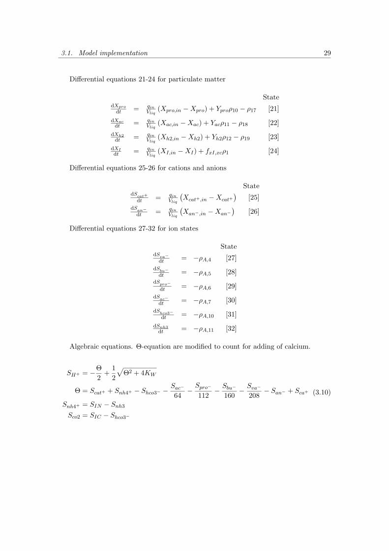
Differential equations 21-24 for particulate matter
StatedXpro
dt = qinVliq
(Xpro,in −Xpro) + Yproρ10 − ρ17 [21]
dXacdt = qin
Vliq(Xac,in −Xac) + Yacρ11 − ρ18 [22]
dXh2dt = qin
Vliq(Xh2,in −Xh2) + Yh2ρ12 − ρ19 [23]
dXIdt = qin
Vliq(XI,in −XI) + fxI,xcρ1 [24]
Differential equations 25-26 for cations and anions
StatedScat+
dt = qinVliq
(Xcat+,in −Xcat+
)[25]
dSan−dt = qin
Vliq
(Xan−,in −Xan−
)[26]
Differential equations 27-32 for ion states
StatedSva−
dt = −ρA,4 [27]dSbu−
dt = −ρA,5 [28]dSpro−
dt = −ρA,6 [29]dSac−
dt = −ρA,7 [30]dShco3−
dt = −ρA,10 [31]
dSnh3dt = −ρA,11 [32]
Algebraic equations. Θ-equation are modified to count for adding of calcium.
SH+ = −Θ2
+12
√Θ2 + 4KW
Θ = Scat+ + Snh4+ − Shco3− −Sac−
64−Spro−
112− Sbu−
160− Sva−
208− San− + Sca+
Snh4+ = SIN − Snh3
Sco2 = SIC − Shco3−
(3.10)

3.1. Model implementation 30
Gas phase equationsDifferential equations
StatedSgas,h2
dt = −Sgas,h2qgasVgas
+ ρT,8 ·VliqVgas
[33]dSgas,ch4
dt = −Sgas,ch4qgasVgas
+ ρT,9 ·VliqVgas
[34]dSgas,co2
dt = −Sgas,co2qgasVgas
+ ρT,10 ·VliqVgas
[35]
Algebraic equations
pgas,h2 = Sgas,h2 ·RTop
16
pgas,ch4 = Sgas,ch4 ·RTop
64pgas,co2 = Sgas,co2 ·RTopPgas = pgas,h2 + pgas,ch4 + pgas,co2 + pgas,h2o
qgas = kp(Pgas − Patm) · PgasPatm
(3.11)
Not standard ADM1 equations Some of the equations above are modified toocount for the added lactate and calcium. But there are also differential equations for thenew substrates as well. Those equations can bee seen here
StatedSlac
dt = qinVliq
(Slac,in − Slac)− ρ20 − ρ21 [36]dXlacf
dt = qinVliq
(Xlacf,in −Xlacf ) + Ylacfρ20 − ρ22 [37]
dXlacodt = qin
Vliq(Xlaco,in −Xlaco) + Ylacoρ21 − ρ23 [38]
dScadt = qin
Vliq(Sca,in − Sca)− ρP,24 [39]
(3.12)
3.1.2 Verifying the implementation
Verifying the model is important, but also time consuming. If not done properly theoutcome of the model will not be valid and simulation results nonsense. Therefore as afirst step files of course were studied carefully in order to find small slips. More significantverifications were done by comparing the outcome of the simulations with the outcomeof Rosen and Jeppssons simulations [4]. Since the indata used in the simulation wasconsistent to the one used in the report by Rosen and Jeppsson the outcome should beequivalent.
To verify the model after adding extra equations for lactate and calcium were thosefirst set to zero and it was controlled that the result still were consistent with the results

3.2. Simulation 31
before adding them. When turning the contribution of the new equations on, there wereno real theoretical equations to compare with, so instead the overall look of the equationswere controlled and testing were left as a verification to do when the model is fitted toa real system.
3.2 Simulation
The model build is used in order to test different scenarios. Compared to do tests ina real situation the flexibility of simulations is endless. In a real life situation it isnot possible to risk the process ongoing in digester tanks in order to test a lot of newsubstrates or other aspects of methane production. But in a simulation environment theaffects can be investigated and conclusions can be drawn to see if new ideas works andwhat outcome of them will be.
3.2.1 Sensitivity analysis
The model is built up by a large system of parameters and variables. For a real lifeadoption of results from simulations to an implementation in a real plant, it is importanthow parameters affects reliability of results. Are there some parameters defining space,in which calculations done, affecting results more than others? If this is the case, it ismore important to study those parameters in order to chose them correctly, comparedto parameters not affecting results equally much.
To study this parameter dependence of the model, produced methane gas were chosenas interesting result outcome from the model. By choosing all parameters as they weresupposed to be and then increasing them 1% at a time, affect of methane productionwere investigated. From those recorded affects in gas production the definition of thederivative (3.13) is possible use to investigate parameter dependency, in the equation isthe parameter denoted by x.
dfdx
=f(x+ ∆h)− f(x)
∆h(3.13)
However in order to do calculations as easy as possible the following is done insteadof using the standard derivative definition
dfdx
=f(1.01x)− f(x)
0.01x(3.14)
By creating a plot with this method for determining sensitivity (using times 1.01instead of ∆h) the plot for parameter dependency, can be considered a one dimensionalJacobian matrix, containing numerical evaluated partial derivatives of gas production,as a function of each parameter investigated. For parameter p1,p2, . . . , pn this can bewritten as
J = [∂qgas,ch4
∂p1,∂qgas,ch4
∂p2, . . . ,
∂qgas,ch4
∂pn] (3.15)

3.2. Simulation 32
Even though this is a logical and easily motivated method used for determining vari-able dependence there will be problems comparing different parameter dependencies toeach others. The denominator in the definition of the derivative is dimensional depen-dent, causing all sensitivities having different dimensions and therefore is comparisonbetween different parameters impossible with this method. Instead a similar methodusing only the numerator in the definition is used. This method is normally referred toas finite difference, having an equation looking like
change in gas production = |f(x · 1.01)− f(x)| (3.16)
Using this method the result will be affected of methane gas production dependingon parameter tested.
An important aspect with this numerical method of calculating parameter depen-dency is that it is only valid in one specific position of parameter space and by changingany of the parameters result is not valid any more and a new analysis is needed to bedone. Which also is the case if input variables defining flow into the model are changed.Those will also affect the parameter space in which calculations are performed.
Therefore it is interesting to compare results of simulations of dependence for differ-ent parts of parameter space. For example if a parameter dependence investigation isperformed before an optimization in gas production is done, this dependence evaluationneeds to be redone after optimization as well to find if there are any changes in parameterdependency.
When input variables are dynamically changed it will cause changes in parametersensitivity as well. To find out how much a shift in input variables cause in outflowfunctions were developed for dynamically changing input variables meanwhile sensitivitywere calculated.
Sensitivity analysis implementationIn order to run the sensitivity analysis described above the following pseudo code canbe applied
• Read indata from file
• Select start values
• Calculate reference gas value for unchanged system, f(x)
• For each interesting parameter do:
– increment parameter value by 1%
– calculate new value of produced gas, f(0.01x)
– calculate change (sensitivity)|f(x+ ∆h)− f(x)| = |f(0.01x)− f(x)|
• Plot result

3.3. Maximizing gas production 33
3.2.2 Variable dependence of parameters
As stated before, parameter dependence calculated, is only valid in one part of parameterspace. However there are sometimes inflows that varies with time. Those flows into thedigester affects the position in parameter space in which calculations are performed. Toget knowledge of what affects this will have on the system sensitivity multiple analysisneeds to be done, one per position investigated. The general dependence of sensitivitycoupled to one variable is therefore investigated by gradually changing inflow meanwhilecalculating sensitivity of interesting parameters.
Simulations of this type are therefore performed with the following method, wherev is variable value, p is parameter value and f(v,p) is the amount of produced CH4 gas(measured as flow [m3/d]) as a function of v,p.
• Read indata
• Chose start values
• Do a finite number of times:
– select new variable value
– calculate gas production, f(v,p)
– increment parameter with 1%
– calculate gas production, f(v,1.01p)
– calculate sensitivity|f(v,1.01p)− f(v,p)|
• Visualize
3.3 Maximizing gas production
One of the goals with the co digestion together with getting rid of the produced manureis to obtain as much gas as possible. To test and verify this the standard way is to do atrial and error search for optimal settings on the digesting process. This is not optimaland hence there need to be a better and more effective way of optimizing the problem.
In this project simulation is used and around the implemented ADM1 model a Parti-cle Swarm Optimization (PSO) [6] framework is build, which can be used to investigateoptimal settings for obtaining as much gas as possible.
Even though the model consists out of a huge number of parameters a large numberof those can not be changed during an optimization method in order to find the optimalgas production. Most of the parameters are fixed and are therefore uninteresting inan optimization algorithm. However are the performed sensitivity analysis of thoseparameters still important in order to know which one of them is most important toobtain reliable results.

3.3. Maximizing gas production 34
The things that can be changed is mixture in the ingoing feed to the digestionchamber, or actually temperature and retention of substrate can be changed as well,but the interesting parts in this project are the mixtures in the ingoing feed. By forexample chancing the fraction between carbon and nitrogen the amount of produced gascan be affected. This then illustrates an adding of manure with a typical fraction ofnitrogen and carbon to already existing fraction of carbon and nitrogen in the standardmanure-free in feed to the digester. There are a lot of variables in the ingoing feed soeven though there are a lot of fixed parameters there still are a large set of variables thatcan be changed during an optimization procedure.
3.3.1 PSO implementation
The dimensions that a particle in PSO can move in will therefore be the concentrationsin the ingoing feed to the digestion chamber and also the amount of flow. The interestingproperty to optimize is the outflow of CH4 and therefore is amount of produced CH4
used as the result of an evaluation of a position in the search space.Normally when implementing an particle swarm optimization method there are fixed
intervals in which the particles can be initialized and then is only the velocity at theparticles controlled by a maximum velocity [6]. However this is not valid in this specificproblem. For example it is only possible to change the mixture in a specific region andtherefore it is not interesting to know if the blending of the mixture is more preferableoutside this region. So therefore is movement of each particle restricted to a region inwhich it is initialized.
An other change made to standard PSO-algorithm presented by [6] is that due to thedifferent dimensions that the particles have is the maximum velocity chosen differently indifferent dimensions. Compared to if the possible propagating dimensions were dimen-sionless and in same magnitude would it be possible to change the different maximumvelocities to one single maximum velocity. But due to the dimensional dependence ofthe space are different maximum velocities chosen.
Pseudo codeThe algorithm used for this implementation of PSO implementation can be seen below,as mentioned above is the target function as high flow of methane gas as possible. Asnoticeable are the positions in search space evaluated and verified to be in the allowedregions. Without those changes the code is an implementation of the proposed PSOimplementation in [6]
• Initialize particles
• Set best global function
• Repeat a finite number of iterations
– for each particle do:
∗ evaluate current value

3.3. Maximizing gas production 35
∗ test if global best (yes -> set as new global best)
∗ test if particle best (yes-> set as new local best)
– for each particle and dimension update:
∗ calculate new velocity
∗ verify velocity < maximum velocity (no -> velocity = maximum ve-locity)
∗ calculate new position
∗ verify min position < position < max position (no -> bring theparticle back to the boundary)
PSO equationsThe pseudo code above can be translated into equations. This is also some sort of pseudocode, but it contains some equations as well. In the code there are a lot of notationsdefined here. The notations follows [6] for maximum readability.
• α - constant in PSO algorithm, often set to 1
• c1 - parameter in PSO algorithms, the term containing c1 is normally referred toas the cognitive component
• c2 - parameter in PSO algorithms, the term containing c2 is normally referred toas the social component
• r and q - random numbers
• N - number of particles
• n - dimensions
• i - particle number (in swarm)
• j - dimension number
• p - particle
• xpbi - local best known position of particle
• xsb - global best known position of the swarm
• ∆t - time step length, for simplicity set to 1
Using this notation one gets:
1. Initialize positions pi for particle i:
(a) xij = xmin + r(xmax − xmin), i = 1, . . . , N, j = 1, . . . , n
(b) vij = α∆t
(−−xmax−xmin2 + r (xmax − xmin)
), i = 1, . . . , N, j = 1, . . . , n

3.4. GUI 36
2. Evaluate each particle in the swarm: f(xi), i = 1, . . . ,N
3. Update best position for each particle and in the swarm: for all particle pi, i =1, . . . , N :
(a) if f(xi) < f(xpbi ) then xpbi ← xi(b) if f(xi) < f(xsb) then xsb ← xi
4. Update particle velocities and positions:
(a) vij ← vij + c1q
(xpbij−xij
∆t
)+ c2r
(xpbj −xij
∆t
), i = 1, . . . , N, j = 1, . . . , n
(b) Restrict velocities so that |vij | < vmax,i
(c) xij ← xij + vij∆t, i = 1, . . . , N, j = 1, . . . , n
(d) Restrict positions so that pmin,j < pij < pmax,j
(e) Return to step 2, unless maximum number of iterations is fulfilled
3.4 GUI
In order to make results of this thesis available for persons not normally working inMATLAB a graphical user interface (GUI) is created. This allows changes to be made tothe simulations without actual chancing in source code of the project.
The GUI it self can not be used to evaluate all possible uses of the model build.The most important use of the model will still be to use it as a framework for newand interesting simulations. The model is ideally used together with some interest insimulating some parts of a system, as for example the optimization process done or thesensitivity analysis described above. Those simulations are built upon the model. Theyuses resources from the model and add something interesting to analysis done. The GUIon the other hand is useful when wanting to test what happens with some set of data asthey are evaluated with help of the model.
3.4.1 Basins of the GUI
The GUI are based on the framework of the model. The only things it adds are abilityto chose inputs and starting values to simulations and the ability to choose plots. Thereare no things that can be controlled from the GUI that not can be controlled from thesource code it self. The GUI is meant to be used by persons unfamiliar to MATLAB butinterested in evaluating the model. The more experienced user are recommend using themodel by building its own simulation based upon the models framework.
The use of the GUI can be seen in the below pseudo code
• Start
• Iterate until shut down:

3.4. GUI 37
– chose start values
– chose variables in inflow
– chose parameters
– if wanted save parameters and variables
– chose plots wanted
– run simulation with selected parameters and variables
– visualize wanted plots
– save or load parameters

4Results
The results presented in this section shows typically results when using the implementedmodel and also results from when the on top of the model implemented simulations arerun. The indata to those simulations and tests are proposed by Rosen and Jeppsson [4]as long as not stated otherwise.
4.1 Model implementation
The implemented model can be used as a stand alone model for testing a specific systemor it can be used as a base for further applications. The framework provided from thisthesis is supposed to be easy to understand and highly adoptable for further applications.It follows the proposed implementation by Rosen and Jeppsson [4] as far as possible inall from nomenclature and notation to structure, however there are changes made to theproposed implementation, but those are described in the Method section, see section 3.
All substrates presented in the model can be seen in table 4.1. From those substratesit is easy to compile plots of simulation results, but also other concentrations are easilycalculated, such as gas pressure, gas flow and pH-values.
For gas pressure just use equations in (2.11) and calculated concentrations of differentgases, from table 4.1. For gas flow use outflow of total gas from model and multiply itwith partial pressure for the investigated type of gas (CH4, CO2 or H2). For pH-values,combine equations (3.5) and (3.10) and use the output from the model.
When running the model with typically values giving rise to steady state solutionsone gets the following plots for the components in model, see figure 4.1 to 4.5 and whencompiling the result in order to get more info out of the data, as described above one getsthe plot in figure 4.6 for produced gas and the plot in figure 4.7 for pH, gas productioncan be seen as gas flow in figure 4.8.

4.1. Model implementation 39
Table 4.1: Substrates in model
Substrate concentration Notation Note
Soluble component sugar Ssu
Soluble component amino acid Saa
Soluble component fatty acid Sfa
Soluble component valerate Sva
Soluble component butyrate Sbu
Soluble component propionate Spro
Soluble component acetate Sac
Soluble component hydrogen Sh2
Soluble component methane Sch4
Soluble component inorganic carbon SIC
Soluble component inorganic nitrogen SIN
Soluble component inerts SI
Particulate component composites Xc
Particulate component carbohydrates Xch
Particulate component proteins Xpr
Particulate component lipids Xli
Particulate component sugar Xsu
Particulate component amino acids Xaa
Particulate component fatty acids Xfa
Particulate component c4 Xc4
Particulate component propionate Xpro
Particulate component acetate Xac
Particulate component hydrogen Xh2
Particulate component inerts XI
Soluble component cations Scat
Soluble component anions San
Soluble component valerate ions Sva-
Soluble component butyrate ions Sbu-
Soluble component propionate ions Spro-
Soluble component acetate ions Sac-
Soluble component hydrogen carbonate Shco3-
Soluble component ammonia ions Snh3
Soluble component hydrogen gas Sgas,h2
Soluble component methane gas Sgas,ch4
Soluble component carbon dioxide gas Sgas,co2
Soluble component lactate Slac Not included in standard ADM1Particulate component lactate fermentation Xlac,f Not included in standard ADM1Particulate component lactate oxidation Xlac,o Not included in standard ADM1Soluble component calcium Sca Not included in standard ADM1

4.1. Model implementation 40
0 5 10 15 20 25 30 35 40 45 50
0.0119
0.0119
0.0119
0.0119
0.0119
0.012
0.012
0.012
0.012
0.012
Ssu
Time [d]
Co
nce
ntr
atio
n [
kg
CO
D/m
3]
0 5 10 15 20 25 30 35 40 45 505.31
5.311
5.312
5.313
5.314
5.315
5.316
5.317
5.318
5.319
5.32x 10
−3S
aa
Time [d]
Co
nce
ntr
atio
n [
kg
CO
D/m
3]
0 5 10 15 20 25 30 35 40 45 500.098
0.0985
0.099
0.0995
0.1
0.1005
0.101
Sfa
Time [d]
Co
nce
ntr
atio
n [
kg
CO
D/m
3]
0 5 10 15 20 25 30 35 40 45 50
0.0116
0.0116
0.0116
0.0117
0.0117
0.0117
Sva
Time [d]
Co
nce
ntr
atio
n [
kg
CO
D/m
3]
0 5 10 15 20 25 30 35 40 45 500.0132
0.0133
Sbu
Time [d]
Co
nce
ntr
atio
n [
kg
CO
D/m
3]
0 5 10 15 20 25 30 35 40 45 50
0.0158
0.0158
0.0158
0.0158
0.0158
0.0159
0.0159
0.0159
Spro
Time [d]
Co
nce
ntr
atio
n [
kg
CO
D/m
3]
0 5 10 15 20 25 30 35 40 45 500
0.5
1
1.5
2
2.5
3
3.5
4
4.5
5
Sac
Time [d]
Concentr
ation [kgC
OD
/m3]
0 5 10 15 20 25 30 35 40 45 502.36
2.365
2.37
x 10−7
Sh2
Time [d]
Co
nce
ntr
atio
n [
kg
CO
D/m
3]
Figure 4.1: Component output from model simulation. Output of substrate number 1-8.Parameters and inflow are defined in appendix B and appendix C.

4.1. Model implementation 41
0 5 10 15 20 25 30 35 40 45 500.05
0.055
0.06
0.065
0.07
0.075
0.08
Sch4
Time [d]
Co
nce
ntr
atio
n [
kg
CO
D/m
3]
0 5 10 15 20 25 30 35 40 45 500.02
0.04
0.06
0.08
0.1
0.12
0.14
0.16
SIC
Time [d]
Concentr
ation [
km
ole
C/m
3]
0 5 10 15 20 25 30 35 40 45 500.13
0.1302
0.1304
0.1306
0.1308
0.131
0.1312
0.1314
0.1316
0.1318
SIN
Time [d]
Co
nce
ntr
atio
n [
km
ole
N/m
3]
0 5 10 15 20 25 30 35 40 45 500
0.05
0.1
0.15
0.2
0.25
0.3
0.35
SI
Time [d]
Concen
tration
[kgC
OD
/m3]
0 5 10 15 20 25 30 35 40 45 500.1025
0.1025
0.1025
0.1025
0.1026
0.1026
0.1026
0.1026
Xc
Time [d]
Co
nce
ntr
atio
n [
kg
CO
D/m
3]
0 5 10 15 20 25 30 35 40 45 500.0293
0.0294
0.0294
0.0295
Xch
Time [d]
Co
nce
ntr
atio
n [
kg
CO
D/m
3]
0 5 10 15 20 25 30 35 40 45 500.4195
0.4196
0.4197
0.4198
0.4199
0.42
0.4201
0.4202
Xpr
Time [d]
Co
nce
ntr
atio
n [
kg
CO
D/m
3]
0 5 10 15 20 25 30 35 40 45 501.1786
1.1787
1.1788
1.1789
1.179
1.1791
1.1792
Xli
Time [d]
Co
nce
ntr
atio
n [
kg
CO
D/m
3]
Figure 4.2: Component output from model simulation. Output of substrate number 9-16.Parameters and inflow are defined in appendix B and appendix C.

4.1. Model implementation 42
0 5 10 15 20 25 30 35 40 45 500.237
0.238
0.239
0.24
0.241
0.242
0.243
0.244
0.245
Xsu
Time [d]
Co
nce
ntr
atio
n [
kg
CO
D/m
3]
0 5 10 15 20 25 30 35 40 45 500.4304
0.4306
0.4308
0.431
0.4312
0.4314
0.4316
0.4318
0.432
Xaa
Time [d]
Co
nce
ntr
atio
n [
kg
CO
D/m
3]
0 5 10 15 20 25 30 35 40 45 500.1363
0.1364
0.1365
0.1366
0.1367
0.1368
0.1369
0.137
0.1371
0.1372
0.1373
Xfa
Time [d]
Co
nce
ntr
atio
n [
kg
CO
D/m
3]
0 5 10 15 20 25 30 35 40 45 500.5
0.55
0.6
0.65
0.7
0.75
0.8
0.85
Xc4
Time [d]
Concen
tration
[kgC
OD
/m3]
0 5 10 15 20 25 30 35 40 45 500.3145
0.315
0.3155
0.316
0.3165
0.317
0.3175
0.318
Xpro
Time [d]
Co
nce
ntr
atio
n [
kg
CO
D/m
3]
0 5 10 15 20 25 30 35 40 45 5025.612
25.613
25.614
25.615
25.616
25.617
25.618
25.619
Xac
Time [d]
Co
nce
ntr
atio
n [
kg
CO
D/m
3]
0 5 10 15 20 25 30 35 40 45 50−1
−0.5
0
0.5
1
1.5
Xh2
Time [d]
Concentr
ation
[km
ole
/m3]
0 5 10 15 20 25 30 35 40 45 50−1
−0.5
0
0.5
1
1.5
Xi
Time [d]
Concentr
ation
[km
ole
/m3]
Figure 4.3: Component output from model simulation. Output of substrate number 17-24.Parameters and inflow are defined in appendix B and appendix C.

4.1. Model implementation 43
0 5 10 15 20 25 30 35 40 45 500.3
0.301
0.302
0.303
0.304
0.305
0.306
0.307
0.308
0.309
0.31
Scat
Time [d]
Co
nce
ntr
atio
n [
kg
CO
D/m
3]
0 5 10 15 20 25 30 35 40 45 500.0279
0.0279
0.0279
0.0279
0.0279
0.0279
0.0279
0.0279
0.0279
0.0279
0.028
San
Time [d]
Co
nce
ntr
atio
n [
kg
CO
D/m
3]
0 5 10 15 20 25 30 35 40 45 50
0.0116
0.0116
0.0116
0.0116
0.0116
0.0117
Sva
−
Time [d]
Co
nce
ntr
atio
n [
kg
Ca
CO
3/m
3]
0 5 10 15 20 25 30 35 40 45 500.0132
0.0133
Sbu
−
Time [d]
Co
nce
ntr
atio
n [
kg
Ca
CO
3/m
3]
0 5 10 15 20 25 30 35 40 45 500.0157
0.0157
0.0157
0.0158
0.0158
0.0158
0.0158
0.0158
0.0159
0.0159
0.0159
Spro
−
Time [d]
Co
nce
ntr
atio
n [
kg
Ca
CO
3/m
3]
0 5 10 15 20 25 30 35 40 45 500
0.5
1
1.5
2
2.5
3
3.5
4
4.5
5
Sac
−
Time [d]
Concentr
ation [kg C
aC
O3/m
3]
0 5 10 15 20 25 30 35 40 45 500.04
0.06
0.08
0.1
0.12
0.14
0.16
Shco3
−
Time [d]
Concentr
ation [
kg
Ca
CO
3/m
3]
0 5 10 15 20 25 30 35 40 45 500
0.02
0.04
0.06
0.08
0.1
0.12
Snh3
Time [d]
Concentr
ation [
kg
Ca
CO
3/m
3]
Figure 4.4: Component output from model simulation. Output of substrate number 25-32.Parameters and inflow are defined in appendix B and appendix C.

4.1. Model implementation 44
0 5 10 15 20 25 30 35 40 45 500.9
0.95
1
1.05
1.1
1.15
1.2
1.25x 10
−5S
gas,h2
Time [d]
Co
nce
ntr
atio
n [
kg
Ca
CO
3/m
3]
0 5 10 15 20 25 30 35 40 45 501.5
1.6
1.7
1.8
1.9
2
2.1
2.2
2.3
2.4
2.5
Sgas,ch4
Time [d]
Concentr
ation [kg C
aC
O3/m
3]
0 5 10 15 20 25 30 35 40 45 500
0.005
0.01
0.015
Sgas,co2
Time [d]
Co
nce
ntr
atio
n [
kg
Ca
CO
3/m
3]
0 5 10 15 20 25 30 35 40 45 50−1
−0.8
−0.6
−0.4
−0.2
0
0.2
0.4
0.6
0.8
1
Slac
Time [d]
Concen
tration
[kgC
OD
/m3]
0 5 10 15 20 25 30 35 40 45 50−1
−0.8
−0.6
−0.4
−0.2
0
0.2
0.4
0.6
0.8
1
Xlac,f
Time [d]
Con
centr
ation [kgC
OD
/m3]
0 5 10 15 20 25 30 35 40 45 50−1
−0.8
−0.6
−0.4
−0.2
0
0.2
0.4
0.6
0.8
1
Xlac,o
Time [d]
Con
centr
ation [kgC
OD
/m3]
0 5 10 15 20 25 30 35 40 45 50−1
−0.8
−0.6
−0.4
−0.2
0
0.2
0.4
0.6
0.8
1
Sca
Time [d]
Concentr
ation [kg
Ca
CO
3/m
3]
Figure 4.5: Component output from model simulation. Output of substrate number 33-39.Parameters and inflow are defined in appendix B and appendix C.

4.1. Model implementation 45
0 5 10 15 20 25 30 35 40 45 50−0.5
0
0.5
1
Time [d]
Pre
ssure
[bar]
Gas pressur
H
2
CH4
CO2
Figure 4.6: Calculated produced gas from model simulation. Parameters and inflow aredefined in appendix B and appendix C.
0 5 10 15 20 25 30 35 40 45 506
7
8
9
10
11
12
13
pH
Time [d]
pH
Figure 4.7: Calculated pH from model simulation. Parameters and inflow are defined inappendix B and appendix C.

4.1. Model implementation 46
0 10 20 30 40 50
10−4
10−2
100
102
Time [d]
Flo
w [
m3
/d]
Gas flow
qgas,total
qgas,h2
qgas,ch4
qgas,co2
qgas,h2o
Figure 4.8: Calculated gas production (outflow from model). To see all flows is the plotdone with logarithmic scale. Parameters and inflow are defined in appendix B and appendixC.

4.1. Model implementation 47
4.1.1 Verifying the implementation
Verification of the model is an important part of the thesis, due to that it verifies thatmodel results are reliable. The verifying is performed by comparing results from modelwith results from Rosen and Jeppssons ADM1 implementation [4]. In the report by Rosenand Jeppsson it is stated that results will not be identically due to different choices ofentire equation systems and individual equations, they should however correspond eventhough perhaps not identically. By running the simulation with identical input as in[4], see C.1 in appendix C and turning concentrations of newly added substrates to zeroone gets exactly the same case as analyzed by Rosen and Jeppsson. The output shouldtherefor correspond, this comparison can be seen in table 4.2.
There are large correlations between the values even though they not are identically.

4.1. Model implementation 48
Table 4.2: Steady state output comparison between [4] and actual model implementation.The input for creating those values can be seen in table C.1
State No. Variable Value [4] Value simulation Difference ratio Unit
1 Ssu 0.0119548297170 0.0119547850647 0.000003735098520 kgCODm – 3
2 Saa 0.0053147401716 0.0053147202657 0.000003745427606 kgCODm – 3
3 Sfa 0.0986214009308 0.0986212138885 0.000001896572681 kgCODm – 3
4 Sva 0.0116250064639 0.0116249647170 0.000003591142082 kgCODm – 3
5 Sbu 0.0132507296663 0.0132506818888 0.000003605663497 kgCODm – 3
6 Spro 0.0157836662845 0.0157836088264 0.000003640365181 kgCODm – 3
7 Sac 0.1976297169375 0.1977953113077 0.000837200685422 kgCODm – 3
8 Sh2 0.0000002359451 0.0000002359449 0.000000847655533 kgCODm – 3
9 Sch4 0.0550887764460 0.0549591519906 0.002358559961445 kgCODm – 3
10 SIC 0.1526778706263 0.1526407718329 0.000243046421703 kmoleCm – 3
11 SIN 0.1302298158037 0.1302298441112 0.000000217365691 kmoleNm – 3
12 SI 0.3286976637215 0.3283360943788 0.001101217164028 kgCODm – 3
13 Xxc 0.3086976637215 0.3086976049107 0.000000190512654 kgCODm – 3
14 Xch 0.0279472404350 0.0279472398610 0.000000020538700 kgCODm – 3
15 Xpr 0.1025741061067 0.1025741055327 0.000000005595954 kgCODm – 3
16 Xli 0.0294830497073 0.0294830488463 0.000000029203221 kgCODm – 3
17 Xsu 0.4201659824546 0.4201659524103 0.000000071505793 kgCODm – 3
18 Xaa 1.1791717989237 1.1791717626995 0.000000030720036 kgCODm – 3
19 Xfa 0.2430353447194 0.2430348264437 0.000002132516181 kgCODm – 3
20 Xc4 0.4319211056360 0.4319209645749 0.000000326590074 kgCODm – 3
21 Xpro 0.1373059089340 0.1373058288317 0.000000583386012 kgCODm – 3
22 Xac 0.7605626583132 0.7605615234530 0.000001492134646 kgCODm – 3
23 Xh2 0.3170229533613 0.3170227140545 0.000000754856953 kgCODm – 3
24 XI 25.6173953274430 25.6173875632640 0.000000303082388 kgCODm – 3
25 Scat 0.0400000000000 0.0400000000000 0 kmolem – 3
26 San 0.0200000000000 0.0200000000000 0 kmolem – 3
- Q 170.00000000000 170.00000000000 0 m 3d – 1
- Top 35.000000000000 35.000000000000 0 ◦C
- pH 7.4655377698929 7.4665935310362 0.000141397966678 -
- SH+ 0.0000000342344 0.0000000341512 0.002436224788587 ◦C
27 Sva- 0.0115962470726 0.0115962750850 0.000002415637763 kgCODm – 3
28 Sbu- 0.0132208262485 0.0132208510214 0.000001873774991 kgCODm – 3
29 Spro- 0.0157427831916 0.0157428248907 0.000002648768584 kgCODm – 3
30 Sac- 0.1972411554365 0.1974073666054 0.000841970448004 kgCODm – 3
31 Shco3- 0.1427774793921 0.1427652639943 0.000085562814499 kmoleCm – 3
- Sco2 0.0099003912343 0.0098755078386 0.002519707958991 kmoleCm – 3
32 Snh3 0.0040909284584 0.0041005728913 0.002351972067235 kmoleNm – 3
- Snh4+ 0.1261388873452 0.1261292712198 0.000076240235966 kmoleNm – 3
33 Sgas,h2 0.0000102410356 0.0000102361173 0.000480484919805 kgCODm – 3
34 Sgas,ch4 1.6256072099814 1.6212531698151 0.002685601636663 kgCODm – 3
35 Sgas,co2 0.0141505346784 0.0141147460189 0.002535551079139 kmoleCm – 3
- pgas,h2 0.0000163991826 0.0000163913070 0.000480474192815 bar
- pgas,ch4 0.6507796328232 0.6490365791240 0.002685601636740 bar
- pgas,co2 0.3625527133281 0.3616357673681 0.002535551078571 bar
- pgas 1.0690164904089 1.0663564828741 0.002494482452651 bar
- qgas∗ 2955.70345419378 2964.86535854150 0.003090158654703 Nm 3d – 1
* = In order to being able to compare the outflow of gas from the model to Rosen and Jepssons result,the calculation of gas flow is changed to atmospheric pressure instead of headspace pressure as normallyused in the model.

4.1. Model implementation 49
0 10 20 30 40 50 60 70 800
2
4
6
8
10
12
14
16
18
X = 15Y = 4.53
Sensitivity
parameter
|f(x
·1.01)−
f(x
)|
X = 25Y = 16.3
X = 26Y = 15.2
X = 13Y = 2.8
Figure 4.9: Sensitivity analysis for ADM1 model, with input to the model from [4]. Pa-rameter values corresponds to values in table 4.3.
4.1.2 Sensitivity analysis
Sensitivity analysis can be performed for different positions in parameter space andresults are depending on which position in space investigated. Therefore the sensitivityanalysis presented here is just a representation of a possible result. To get adequateresults for a specific implementation it is crucial to do a new sensitivity analysis forthat case. Sensitivity is measured in affect of produced methane through numericalcalculation of derivative or finite difference, see section 3.2.1 for further explanation.
The parameters used when doing the sensitivity analysis presented here comes from[4]. Variables and parameters used can be seen in table C.1 (variables) and in appendixB (parameters). Outgoing from those are the sensitivity analysis in figure 4.9 created.On the figures x-axis a lot of parameters are presented as numbers, those numbers canbe coupled to a parameter by table 4.3.

4.1. Model implementation 50
Table 4.3: Parameter denomination in sensitivity analysis plot. The number in the tablecorresponds to a position on the x-axis in figure 4.9.
Number Parameter Number Parameter Number Parameter
1 fsI,xc 26 Patm 51 KS,ac
2 fxI,xc 27 kp 52 KI,nh3
3 fch,xc 28 kL,a 53 pHUL,ac
4 fpr,xc 29 Vgas 54 pHLL,ac
5 fli,xc 30 kdis 55 km,h2
6 fh2,su 31 khyd,ch 56 KS,h2
7 fbu,su 32 khyd,pr 57 pHUL,h2
8 fpro,su 33 khyd,li 58 pHLL,h2
9 fac,su 34 KS,IN 59 kdec,X,su
10 Ysu 35 km,su 60 kdec,X,aa
11 fh2,aa 36 KS,su 61 kdec,X,fa
12 fva,aa 37 pHUL,aa 62 kdec,X,c4
13 fbu,aa 38 pHLL,aa 63 kdec,X,ac
14 fpro,aa 39 km,aa 64 kdec,X,h2
15 fac,aa 40 KS,aa 65 km,lac,f
16 Yaa 41 km,fa 66 KS,lac,f
17 Yfa 42 KS,fa 67 km,lac,o
18 Yc4 43 KI,h2,fa 68 KS,lac,o
19 Ypro 44 km,c4 69 KI,h2,lac,o
20 Yac 45 KS,c4 70 KI,vfa
21 Yh2 46 KI,h2,c4 71 kdec,X,lac,f
22 Ylac,f 47 km,pro 72 kdec,X,lac,o
23 Ylac,o 48 KS,pro 73 KS,p,caco3
24 Tbase 49 KI,h2,pro 74 Kr,caco3
25 Top 50 km,ac

4.1. Model implementation 51
4.1.3 Variable dependence
The sensitivity analysis done is only valid in one part of parameter space. To get infor-mation about what happens if the position is changed by changes in inflow is method fortesting this produced. This method varies one or more variables meanwhile sensitivityis plotted for one or more parameters.
For illustrating a typically result when doing this is the plot in figure 4.10 con-structed. The plot illustrates change in sensitivity for two parameters when the amountof inorganic nitrogen in inflow is changed. To do this analysis are the inflow of particu-lates changed from Rosen and Jeppssons choice of variables C to no inflow of particulatecomponents except Xxc, which were changed to 2.0 kg COD m−3.
The result plotted can be a bit hard to read out of figures, due to fluctuations. So tomake it more easy to identify tendencies is also a 50 point average plotted, as a red lineabove the others. The averaging is performed be using the function smooth in MATLAB,which makes an average over surrounding points. The slopes of those lines indicatesoverall change of sensitivity for investigated parameters.
From the plot it is shown that there seems to be something interesting happening inthe region between 0-1 kmoleNm−3, so therefore is a new plot done in this region, seefigure 4.11. This is the way in which the simulation of variable dependence is supposedto be used; Start by choosing a large interval and then look carefully at the intervalin which there seams to happen something interesting. As a result of this more carefulinvestigation on the interval 0-1, it can be seen that the sensitivity are large in a smallinterval around 0.05 kmoleNm−3.
4.1.4 Maximizing gas production
In order to maximizing gas production it is important to notice that there are multiplevariables possible to modified. Due to the objective function chosen, maximizing gasproduction, it is possible that different parts of the system will cancel out positive affectsdone by other parts of the same system.
The affect of this is that all interesting parameters needs to be optimized at sametime to find an optimal choice, which is done by PSO. Results of the PSO algorithmchosen are limited to a predefined range for all variables, which easily can be modify tofir different dimensions.
As mentioned before the optimal mixture found by this process is only valid in onepart of the parameter space, so by changing the parameters, the optimization processneeds to be redone.
In order to build a so useful method as possible, a method allowing changes to bedone in any dimension wanted were created. The method allows ranges to be individuallydefined for all substrates presented in the model. The ranges are actually also possible toset to a finite value if one not wants to optimize in any of the dimensions presented. Theresult presented here shows how the optimal mixture of three different input variablespropagates during a simulation and how the resulting gas production is changed duringthe simulation, see figure 4.12. In the simulation there are 20 PSO particles used and

4.1. Model implementation 52
0 1 2 3 4 5 6 7 8 9 1010
−6
10−4
10−2
100
SIN
[kmole N m−3
]
Se
nsitiv
ity
Sensitivity of KS,IN
and KI,nh3
as a function of SIN
K
S,IN
50 points average
0 1 2 3 4 5 6 7 8 9 1010
−6
10−4
10−2
100
SIN
[kmole N m−3
]
Se
nsitiv
ity
K
I,nh3
50 points average
Figure 4.10: Variable dependence of sensitivity for two parameters. Sensitivity is con-stantly tested meanwhile a variable is changed. In this case the variable changed is SIN
meanwhile KS,IN and KI,nh3 are investigated during this process. The fluctuating of thecurve is reduced by a 50-point average plotted above the curves, showing the trend of theparameters. The values in the simulation are as explained in section 4.1.3.
the simulation was let run until it had reached the boundaries of the box, which were[0,1] kmole/m3 for N,C and [100,200] m3/d for the flow.
In the plot it is possible to see that the optimal position not lies in the selectedinterval, due to that the particles did not reached a best position inside the boundaries,instead the particles were relocated to the boundaries. In order to find the theoreticalbest position, the interval therefore needs to be extended so that a best position ispossible to find inside the interval.
4.1.5 GUI
For people not that skilled in MATLAB a basic GUI is create. In this GUI it is onlypossible to run the model and change variables and parameters. There is no possibilitiesto do the more advanced simulations build upon the model, such as PSO or sensitivityanalysis, but all standard plots of substrates concentrations presented in this report are

4.1. Model implementation 53
0 0.1 0.2 0.3 0.4 0.5 0.6 0.7 0.8 0.9 110
−6
10−4
10−2
100
SIN
[kmole N m−3
]
Se
nsitiv
ity
Sensitivity of KS,IN
and KI,nh3
as a function of SIN
K
S,IN
50 points average
0 0.1 0.2 0.3 0.4 0.5 0.6 0.7 0.8 0.9 110
−6
10−4
10−2
100
SIN
[kmole N m−3
]
Se
nsitiv
ity
K
I,nh3
50 points average
Figure 4.11: Variable dependence of sensitivity for two parameters. Sensitivity is con-stantly tested meanwhile a variable is changed. In this case the variable changed is SIN
meanwhile KS,IN and KI,nh3 are investigated during this process. The fluctuating of thecurve is reduced by a 50-point average plotted above the curves, showing the trend of theparameters. The values in the simulation are as explained in section 4.1.3.
possible to draw and also some additional plots are possible to draw.It is also possible to save sets of analyzed parameters and variables for further use
and of course also load old saved sets. From start the model is loaded with the defaultvalues used in this report.
The main window in the GUI looks like figure 4.13 and by pressing each of the lowerleft buttons different sets of parameters can be set in new windows. The tables in themain windows consists of start values (the mixture in the digestion chamber at start) andinflow values (what the flow into the chamber consists of). The plot selection part of theGUI makes it possible to see how concentrations for substrates varies during simulation.By activating any (one or more) of the boxes the run button becomes active and themodel can be analyzed. Each of the plots shows up in a new own window.

4.1. Model implementation 54
0 5 10 15 20 25 30 35 400
0.2
0.4
0.6
0.8
1
SIC
Number of updates
km
ole
C/m
3
0 5 10 15 20 25 30 35 400
0.2
0.4
0.6
0.8
SIN
Number of updates
km
ole
N/m
3
0 5 10 15 20 25 30 35 40150
160
170
180
190
200
q
Number of updates
Flo
w [m
3/d
]
0 5 10 15 20 25 30 35 400
500
1000
1500
2000
Gas flow − CH4
Number of updates
Ga
s flo
w [m
3/d
]
Figure 4.12: Propagation of optimal mixture in invariable to PSO optimization of gasproduction. The parameters are chosen according to appendix B and the inflow values tothe simulation are defined in C.

4.1. Model implementation 55
Figure 4.13: Main window in GUI.

5Discussion
All discussion for time consumptions done here is depending on the computer used. Theresults presented here are done on a MacBook Pro with a 2.53 GHz Intel Core 2 Duoprocessor and 4 GB 1067 MHz RAM.
5.1 Model implementation
The model implemented can be used as a stand alone model to test different inputs in adigestion chamber. The typical results from this type of test are presented in the reportand also compared to Rosen and Jeppsons results [4]. An interesting part of the usabilityof the model is that combination of start values and steady state infeeds.
During testing phase of the model a large range of start values were tested andevaluated and the results of them were compared to see if the model is robust enoughto handle different kinds of inputs by itself. The results of those simulations were thatthe model seemed to handle different start values in a good way.
By setting unknown concentrations of ions to zero the model was self correcting forproblems in the balance of anions and cations. This is a good behavior of the modeldue to it makes it possible to handle problems with correct start values in an easy andeffective way.
The time it took to run a standard simulation was around three seconds, dependingon the complexity of the choices of the model parameters and how long from steady statethe start was. The model as it is implemented uses the ODE-solver ode15s in MATLAB,which is a smart solver that uses different step length depending on stiffness of problemsand complexity of concentration curves.

5.2. Verifying the implementation 57
5.2 Verifying the implementation
By using the same infeeds as Rosen and Jeppsson[4] the correctness of the present simu-lation were evaluated. The solutions for different substrates do not vary much comparedto Rosen and Jeppssons results. The largest difference is around 3% and every other issmaller and all solutions are therefore considered as good solutions.
5.3 Sensitivity analysis
The sensitivity method produced during the thesis gives clues on which parts that areimportant in a real world situation when implementing the model to an existing plant.The method gives clues on which parameters that are important to choose correctly dueto their effect on the final result.
The method used for performing sensitivity analysis is a finite difference method.The more mathematical logical method using the definition of the derivative requiresdimensionless units and due to that the model is built up with dimensional properties itis easier to keep working with dimensions and therefore the method used is dimensionaldependent.
The results are obtained by changeling each parameter 1% at a time and then cal-culate the effect on methane gas production with the new parameter set obtained. Inorder to visualize the results a bar graph is compiled, which can be seen in figure 4.9.If there are parameters equivalent to zero in the standard parameter set, those are keptzero at comparison implying no measurable change.
Large bars for measured sensitivity correlates to important parameters in the imple-mentation. Those parameters are therefore more important to measure correctly whenthe model is implemented to a real situation.
The time consumption of doing a sensitivity analysis depends on how many parame-ters that are investigated, but normally it takes around three seconds per parameter tobe evaluated and three seconds for the reference as well. So by simple math it is possibleto calculate the time consumption.
5.4 Variable dependence
The sensitivity analysis done in this work is only valid in one position in parameter space.The drawback of this is clear, if one variable in infeed is changed, the entire sensitivityanalysis needs to be redone. Therefor it is interesting to see how the sensitivity changeswith changing variables. For this a framework is implemented. To test this framework,only one variable were changed meanwhile the sensitivity for two different parameterswere evaluated and plotted.
It was supposed that the sensitivity for the two parameters (KS,IN and KI,nh3) woulddecrease with increased values of the variable (SIN ). The reason to suppose this camefrom the project participate Karin Willquist at SP. To test if this was possible to see,firstly a large interval was created and evaluated, see figure 4.10. This did not show

5.5. Maximizing gas production 58
much more than noise and a relatively constant signal (notice the logarithmic y-axis).But there seemed to be something interesting in the low region around 0.5 kmole N m−3.So a second figure was created, see figure 4.11, to investigate this interval and here itwas possible to see that something is happening in this region, larger values of SIN willcontribute to less sensitivity of the parameters, as expected.
The test done indicates that the method to investigate variable dependence of pa-rameters can be done in a clear and understandable manner.
The time consumption for doing the analysis is relatively large. In the analyzedinterval were 1000 points investigated, and by doing three analyses at each point (oneper parameter and one reference) 3000 evaluations of the model were performed. Thetime consumptions of those investigations varied depending on position in space. Someinvestigations took about 20 seconds and some about 2 seconds, leading to a total timeconsumption of about 3 hours.
5.5 Maximizing gas production
The goal of the entire project is to minimize waste from keeping animals meanwhilethe gas production in digestion chambers is increased. To achieve this it is importantto investigate which is the most preferable mixture into the digester, in order to getas much gas out as possible. To know this the normal working manner is a trail anderror procedure. In order to make the search more effective an optimization frameworkis implemented on top of the ADM1 model.
The optimization framework chosen is Particle Swarm Optimization (PSO). Thereason for choosing PSO in front of other methods is that very little about the problemneeds to be known. The only thing needed is a function value for each position in searchspace and in this case amount of produced methane was chosen as wanted quantity tooptimize against.
The chosen algorithm is not the fastest possible and it might not ever find the optimalsolution, due to that it can be trapped inside a local maximum, but it is however asmart algorithm that allows for optimization of a large set of variables simultaneously.Compared to optimize in each dimension, one at the time, this is a far better alternative,depending on that different quantities affect each others. So by using PSO the globalbest combination can be found.
The result presented here, in figure 4.12, shows how the solution propagates to thebest possible solution. To compute the picture three different dimensions were chosenand the solution were plotted to get a feeling on how the algorithm works. Comparedto doing a real simulation where the only output will be the now best known positionthis is a god way of illustrating how the simulation works. However in a real situationthe actual best found mixture in numbers is more interesting and therefore the plots areonly constructed to get a feeling for the algorithm and its propagation.
The amount of possible things to optimize as the method is written are all inputvariables along with the flow. The algorithm does not need to be rewritten to count fordifferent sets of variables to optimize in. The only corrections needed to be done are

5.6. GUI 59
choosing the intervals in which the concentrations lies to be fixed values (for things thatnot are interesting to optimize in) or a finite interval (for thing that one are interestingto optimize).
The time consumption for the PSO method varies depending on what is optimizedand how many steps needed for convergence, but also randomly chosen start positionsin search space effects the simulation time. As before each simulation takes about threeseconds and it seams sufficient to use about 20 particles in the optimization implyingthe initialization process to taking around one minute and then the actual process takesfar more time. About 10-20 minutes were used when testing the method.
5.6 GUI
The GUI constructed is for people not experienced in MATLAB. The possibilities to dothings in the GUI are limited, but there are possibilities to do all basic simulations of themodel. However the more advanced features, with the constructed ADM1 framework,are for people understanding what the simulations does and therefor this is not includedinside the GUI.
The output from the GUI is exactly the same as one gets when using the modelin own simulations, with one major difference. In the GUI the only thing possible toobtain is the plots for different substrates and when using the model in MATLAB onegets substrate concentrations as well. Those substrate concentrations can be used for awide range of things, for example plotting, but also a lot of other things that not canbe done with help of the GUI. On the other hand, the GUI can be run without havingaccess to MATLAB. By compiling the GUI in an Windows environment and packing theMATLAB Compiler Runtime - mcr [8] with the executable file everyone can run the file,regardless if they have a MATLAB license or not.
Time consumption varies with what is being done. If it is a complex system thatis being solved it will take more time and if it is a simple system it will take less. Butaround three seconds per run is what was measured during execution.
5.7 Usability of results
The results of this thesis are mostly in the methods that can be used to test and verifydifferent mixtures in a digesting process. The process itself is only tested in terms oftypical data of which the correctness is not verified in this thesis. To get real usage of themethods the process needs to be fitted to the specific case in each process. This fittingprocess is performed in multiple steps of which fitting the parameters to the actual caseis the first step. When this is done, verifying the implementation is another importantstep that needs to be performed to achieve correct and reliable results.
When fitting the model to processes, the knowledge about sensitivity parameters areimportant due to their affect on the final result.
The functions and methods developed during this thesis will be used in the graterproject on manure in Boras. However this is not part of the thesis and therefor not

5.8. Further development 60
included in this report.
5.8 Further development
5.8.1 Fitting the model to the project
In order to use the methods created it is important to know about the systems that itis supposed to be used on. This requires some lab analysis to be done and also someconverting to standard ADM1 units, that not always are the same as used in lab scaleexperiments. By doing this the model can be used to test and verify the usability ofdifferent raw materials for digesting processes.
5.8.2 Building more methods and simulations
There is an important bit of programming that needed to be done and it is implementingpossibilities to choose different amount of mixtures between manure and standard wastewater sludge as infeeds to the model. As the case is now it is possible to change differentamounts of substrate concentrations in the infeed. But to really get a lot out of the modeldifferent manure types needs to be tested and then those results needs to be convertedto substrates that can be added to the standard in feeds.
By changing the amount of added manure to the infeed the affect of adding manurecan be investigated and an optimal mixture be found. Those analyses has not beenperformed at the moment and therefore are those parts not done in this thesis. At themoment this can be implemented by firstly chancing the concentrations that works asinfeed to the model.
It is proposed that a framework that uses two set of variables, one for the manureand one for the waste water, are developed. By then defining a level of mixing betweenthose sets of variable the actual infeed to the digester can be determined.

6Conclusion
An anaerobic digestion system is mathematically described and implemented using ADM1model, with some small changes done. On top of this modeling system several simula-tions are implemented, evaluating for example stability of process and optimal mixture.All of those systems are implemented using MATLAB.
To increase usability of system the way the model is implemented follows Rosen andJeppssons [4] implementation. However also some additional equations added, those arealso presented in the same way.
For unexperienced MATLAB-users there is a GUI developed that implements and runsthe model as written.
The execution time varies between different simulations and systems but the averagetime consumed to evaluate one set of variables and parameters is three seconds, on aMacBook Pro with a 2.53 GHz Intel Core 2 Duo processor and 4 GB 1067 MHz RAM.

Bibliography
[1] J. I. for jordbruks-och miljoteknik, Energiproduktion med hastgodsel - fran godsel tillvarme pa 4 dagar, http://www.bioenergiportalen.se/?p=6527&m=1723 (04 2014).URL http://www.bioenergiportalen.se/?p=6527&m=1723
[2] P. Wennerberg, C. Dahlander, Hastgodsel som en resurs - en forstudie om olikahanteringskedjor for hastgodsel, Tech. rep. (2013-05-07).
[3] D. Batstone, J. Keller, R. Angelidaki, S. Kalyuzhnyi, S. Pavlostathis, A. Rozzi,W. Sanders, H. Siegrist, V. Vavilin, Anaerobic digestion model no1, isbn:1900222787, Tech. rep. (2002).
[4] C. Rosen, U. Jeppsson, Aspects on adm1 implementation within the bsm2 framework,Tech. Rep. 7224, Dept. of Industrial Electrical Engineering and Automation, LundInstitute of Technology (2005).
[5] K. Willquist, V. N. Nkemka, H. Svensson, S. Pawar, M. Ljunggren, H. Karlsson,M. Murto, C. Hulteberg, E. W. van Niel, G. Liden, Design of a novel biohythaneprocess with high {H2} and {CH4} production rates, International Journal ofHydrogen Energy 37 (23) (2012) 17749 – 17762.URL http://www.sciencedirect.com/science/article/pii/S0360319912019428
[6] M. Wahde, Biologically inspired optimization methods, WIT Press, Southampton,UK.
[7] H. Rylander, W. Wiqvist, Substrahandbok for biogasproduktion, Report, AvfallSverige, Malmo (Jun 2009).
[8] I. The MathWorks, Matlab compiler runtime (mcr),http://www.mathworks.se/products/compiler/mcr/ (04 2014).URL http://www.mathworks.se/products/compiler/mcr/
[9] S. S. Johansson, Modelling of step response in modelling of step response in anaerobicdigesters, Msc. thesis (May 2012).

ABiochemical Rate Matrix
In order to fit the biochemical rate matrices to the pages in this report are the sidesmade blank, meanwhile they also are rotated 90 degrees. To achive this are the matricesplaced at own pages, so to see them continue to next page.

Tab
leA
.1:
Bio
chem
ical
rate
coeffi
cien
t(ν
i,j)
and
kine
tic
rate
equa
tion
s(ρ
j)
for
solu
ble
com
pone
nts.
The
mat
rix
com
esfr
omth
eta
skre
port
[3]
wit
hco
mpl
emen
ting
equa
tion
sfr
omW
illqu
ist
etal
.[5]
Com
ponent→
i1
23
45
67
89
10
11
12
Rate
(ρ
jkgC
OD
mm
–3·d
–1)
jP
rocess↓
Ssu
Saa
Sfa
Sva
Sbu
Spro
Sac
Sh2
Sch4
SIC
SIN
SI
1D
isin
tegra
tion
fsl
,xc
kdis
Xc
2H
ydro
lysi
sofcarb
ohydra
tes
1khyd,c
hX
ch
3H
ydro
lysi
sofpro
tein
s1
khyd,p
rX
pr
4H
ydro
lysi
soflipid
s1
-ffa
,li
ffa
,li
khyd,liX
li
5U
pta
ke
ofsu
gar
-1(1
-Ysu
)fbu,s
u(1
-Ysu
)fpro
,su
(1-Y
su)f
ac,s
u(1
-Ysu
)fh2,s
u−
Pi=
1−
9,
11−
29
Ciν
i,5
-(Y
su)N
bac
km
,su
s su
Ks+
Ssu
Xsu
I 1
6U
pta
ke
ofam
ino
acid
s-1
(1-Y
aa)f
va,a
a(1
-Yaa)f
bu,a
a(1
-Yaa)f
pro
,aa
(1-Y
aa)f
ac,a
a(1
-Yaa)f
h2,a
a−
Pi=
1−
9,
11−
29
Ciν
i,6
Naa-(
Yaa)N
bac
km
,aa
s aa
Ks+
Saa
XaaI 1
7U
pta
ke
ofLC
FA
-1(1−
Yfa
)0.7
(1−
Yfa
)0.3
-(Y
fa)N
bac
km
,fa
s fa
Ks+
Sfa
Xfa
I 2
8U
pta
ke
ofvale
rate
-1(1−
Yc4)0.5
4(1−
Yc4)0.3
1(1−
Yc4)0.1
5-(
Yc4)N
bac
km
,c4
s va
Ks+
Sva
Xc4
11+
Sbu
/Sva
I
9U
pta
ke
ofbuty
rate
-1(1−
Yc4)0.8
(1−
Yc4)0.2
-(Y
c4)N
bac
km
,c4
s bu
Ks+
Sbu
Xc4
11+
Sva
/Sba
I
10
Upta
ke
ofpro
pio
nate
-1(1−
Ypro
)0.5
7(1−
Ypro
)0.4
3−
Pi=
1−
9,
11−
29
Ciν
i,1
0-(
Ypro
)Nbac
km
,pr
s pro
Ks+
Spro
Xpro
I 2
11
Upta
ke
ofaceta
te-1
(1−
Yac)−
Pi=
1−
9,
11−
29
Ciν
i,1
1-(
Yac)N
bac
km
,ac
s ac
Ks+
SacX
acI 3
12
Upta
ke
ofhydro
gen
-1(1−
Yh2)−
Pi=
1−
9,
11−
29
Ciν
i,1
2-(
Yh2)N
bac
km
,h2
s h2
Ks+
Sh2
Xh2I 1
13
Decay
ofX
sukdec,X
suX
su
14
Decay
ofX
aa
kdec,X
aaX
aa
15
Decay
ofX
fakdec,X
faX
fa
16
Decay
ofX
c4
kdec,X
c4X
c4
17
Decay
ofX
pro
kdec,X
pro
Xpro
18
Decay
ofX
ac
kdec,X
acX
ac
19
Decay
ofX
h2
kdec,X
h2X
h2
20
Upta
ke
ofla
cta
te(f
er.
)(1−
Yla
c,f)0.7
85
(1−
Yla
c,f)0.2
15
−P
i=
1−
9,
11−
29
Ciν
i,2
0-(
Yla
c,f)N
bac
km
,lacf
Sla
cK
s+
Sla
cX
lacfI
21
Upta
ke
ofla
cta
te(o
x.)
(1−
Yla
c,o
)2 3
(1−
Yla
c,o
)1 3
−P
i=
1−
9,
11−
29
Ciν
i,2
1-(
Yla
c,o
)Nbac
km
,laco
Sla
cK
s+
Sla
cX
lacoI 2
22
Decay
ofX
lac,f
kdec,X
lacfX
lacf
23
Decay
ofX
lac,o
kdec,X
lacoX
laco
24
Pre
cip
itati
on
ofC
alc
ium
kr,C
aC
o3
“ q Sca·S
hco3−p K
spC
aC
o3
” 2
Monosaccharides(kgCOD·m–3)
Aminoacids(kgCOD·m–3)
Longchainfattyacids(kgCOD·m–3)
Totalvalerate(kgCOD·m–3)
Totalbutyrate(kgCOD·m–3)
Totalpropionate(kgCOD·m–3)
Totalacetate(kgCOD·m–3)
Hydrogengas(kgCOD·m–3)
Methanegas(kgCOD·m–3)
Inorganiccarbon(kmoleC·m–3)
Inorganicnitrogen(kmoleN·m–3)
Solubleinerts(kgCOD·m–3)
Inhib
itio
nfa
cto
rs:
I 1− −
I pH
I IN
,lim
I 1− −
I pH
I IN
,lim
I h2
I 1− −
I pH
I IN
,lim
I NH
3,X
ac

Tab
leA
.2:
Bio
chem
ical
rate
coeffi
cien
t(ν
i,j)
and
kine
tic
rate
equa
tion
s(ρ
j)
for
solu
ble
com
pone
nts.
The
mat
rix
com
esfr
omth
eta
skre
port
[3]
wit
hco
mpl
emen
ting
equa
tion
sfr
omW
illqu
ist
etal
.[5]
Com
ponent→
i13
14
15
16
17
18
19
20
21
22
23
24
36
37
38
39
Rate
(ρ
jkgC
OD
mm
–3·d
–1)
jP
rocess↓
Xc
Xch
Xpr
Xli
Xsu
Xaa
Xfa
Xc4
Xpro
Xac
Xh2
XI
Sla
cX
lac,f
Xla
c,o
Sca
1D
isin
tegra
tion
-1fch
,xc
fpr,xc
fli,x
cfxI,xc
kdis
Xc
2H
ydro
lysi
sofcarb
ohydra
tes
-1khyd,c
hX
ch
3H
ydro
lysi
sofpro
tein
s-1
khyd,p
rX
pr
4H
ydro
lysi
soflipid
s-1
khyd,liX
li
5U
pta
ke
ofsu
gar
Ysu
km
,su
s su
Ks+
Ssu
Xsu
I 1
6U
pta
ke
ofam
ino
acid
sY
aa
km
,aa
s aa
Ks+
Saa
XaaI 1
7U
pta
ke
ofLC
FA
Yfa
km
,fa
s fa
Ks+
Sfa
Xfa
I 2
8U
pta
ke
ofvale
rate
Yc4
km
,c4
s va
Ks+
Sva
Xc4
11+
Sbu
/Sva
I
9U
pta
ke
ofbuty
rate
Yc4
km
,c4
s bu
Ks+
Sbu
Xc4
11+
Sva
/Sba
I
10
Upta
ke
ofpro
pio
nate
Ypro
km
,pr
s pro
Ks+
Spro
Xpro
I 2
11
Upta
ke
ofaceta
teY
ac
km
,ac
s ac
Ks+
SacX
acI 3
12
Upta
ke
ofhydro
gen
Yh2
km
,h2
s h2
Ks+
Sh2
Xh2I 1
13
Decay
ofX
su1
-1kdec,X
suX
su
14
Decay
ofX
aa
1-1
kdec,X
aaX
aa
15
Decay
ofX
fa1
-1kdec,X
faX
fa
16
Decay
ofX
c4
1-1
kdec,X
c4X
c4
17
Decay
ofX
pro
1-1
kdec,X
pro
Xpro
18
Decay
ofX
ac
1-1
kdec,X
acX
ac
19
Decay
ofX
h2
1-1
kdec,X
h2X
h2
20
Upta
ke
ofla
cta
te(f
er.
)-1
Yla
cf
km
,lacf
Sla
cK
s+
Sla
cX
lacfI
21
Upta
ke
ofla
cta
te(o
x.)
-1Y
laco
km
,laco
Sla
cK
s+
Sla
cX
lacoI 2
22
Decay
ofX
lac,f
1-1
kdec,X
lacfX
lacf
23
Decay
ofX
lac,o
1-1
kdec,X
lacoX
laco
24
Pre
cip
itati
on
ofC
alc
ium
-1kr,C
aC
o3
“ q Sca·S
hco3−p K
spC
aC
o3
” 2
Composites(kgCOD·m–3)
Carbohydrates(kgCOD·m–3)
Proteins(kgCOD·m–3)
Lipids(kgCOD·m–3)
Sugardegraders(kgCOD·m–3)
Aminoaciddegraders(kgCOD·m–3)
LCFAdegraders(kgCOD·m–3)
Valerateandbutyratedegraders(kgCOD·m–3)
Propionatedegraders(kgCOD·m–3)
Acetatedegraders(kgCOD·m–3)
Hydrogendegraders(kgCOD·m–3)
Particulateinerts(kgCOD·m–3)
Totallactate(kgCOD·m–3)
Lactate(fermentation)degraders(kgCOD·m–3)
Lactate(oxidation)degraders(kgCOD·m–3)
Totalcalcium(kmole·m–3)
Inhib
itio
nfa
cto
rs:
I 1− −
I pH
I IN
,lim
I 1− −
I pH
I IN
,lim
I h2
I 1− −
I pH
I IN
,lim
I NH
3,X
ac

BModel parameters
The model consist out of a lot of parameters. Those parameters are defined in thefollowing tables. The values in the tables comes from Rosen and Jeppsons report [4]about how to implement the ADM1 model. If nothing else is said in the report thoseparameter values are used for all parameters in this work. Those tables have the numbersB.1 to B.4.
Besides the parameters for the standard ADM1 there are also parameters for thenew substrates added. Those parameter values comes from the master thesis report bySamuel Scherman Johansson[9], those values can be seen in table B.5 to B.7.
B.1 Standard ADM1 parameters

B.1. Standard ADM1 parameters 67
Table B.1: Stoichiometric parameter values (standard ADM1). The structure follows theone in Rosen and Jeppssons report [4] for maximum readability.
Parameter Value UnitfsI,xc 0.1 -fxI,xc 0.2 -fch,xc 0.2 -fpr,xc 0.2 -fli,xc 0.2 -Nxc 0.0376/14 kmole N(kg COD)−1
NI 0.06/14 kmole N(kg COD)−1
Naa 0.007 kmole N(kg COD)−1
Cxc 0.02786 kmole C(kg COD)−1
CsI 0.03 kmole C(kg COD)−1
Cch 0.0313 kmole C(kg COD)−1
Cpr 0.03 kmole C(kg COD)−1
Cli 0.022 kmole C(kg COD)−1
CxI 0.03 kmole C(kg COD)−1
Csu 0.0313 kmole C(kg COD)−1
Caa 0.03 kmole C(kg COD)−1
ffa,li 0.95 -Cfa 0.0217 kmole C(kg COD)−1
fh2,su 0.19 -fbu,su 0.13 -fpro,su 0.27 -fac,su 0.41 -Nbac 0.08/14 kmole N(kg COD)−1
Cbu 0.025 kmole C(kg COD)−1
Cpro 0.0268 kmole C(kg COD)−1
Cac 0.0313 kmole C(kg COD)−1
Cbac 0.0313 kmole C(kg COD)−1
Ysu 0.1 -fh2,aa 0.06 -fva,aa 0.23 -fbu,aa 0.26 -fpro,aa 0.05 -fac,aa 0.40 -Cva 0.024 kmole C(kg COD)−1
Yaa 0.08 -Yfa 0.06 -Yc4 0.06 -Ypro 0.04 -Cch4 0.0156 kmole C(kg COD)−1
Yac 0.05 -Yh2 0.06 -

B.1. Standard ADM1 parameters 68
Table B.2: Biochemical parameter values (standard ADM1). The structure follows theone in Rosen and Jeppssons report [4] for maximum readability.
Parameter Value Unitkdis 0.5 d−1
khyd,ch 10 d−1
khyd,pr 10 d−1
khyd,li 10 d−1
KS,IN 1e-4 Mkm,su 30 d−1
KS,su 0.5 kg COD m−3
pHUL,aa 5.5 -pHLL,aa 4 -km,aa 50 d−1
KS,aa 0.3 kg COD m−3
km,fa 6 d−1
KS,fa 0.3 kg COD m−3
KIh2,fa 5e-6 kg COD m−3
km,c4 20 d−1
KS,c4 0.2 kg COD m−3
KIh2,c4 1e-5 kg COD m−3
km,pro 13 d−1
KS,pro 0.1 kg COD m−3
KIh2,pro 3.5e-6 kg COD m−3
km,ac 8 d−1
KS,ac 0.15 kg COD m−3
KI,nh3 0.0018 kg COD m−3
pHUL,ac 7 -pHLL,ac 6 -km,h2 35 d−1
KS,h2 7e-6 kg COD m−3
pHUL,h2 6 -pHLL,h2 5 -kdec,Xsu 0.02 d−1
kdec,Xaa 0.02 d−1
kdec,Xfa 0.02 d−1
kdec,Xc4 0.02 d−1
kdec,Xpro 0.02 d−1
kdec,Xac 0.02 d−1
kdec,Xh2 0.02 d−1

B.1. Standard ADM1 parameters 69
Table B.3: Physiochemical parameter values (standard ADM1). The structure follows theone in Rosen and Jeppssons report [4] for maximum readability.
Parameter Value Unit
R 0.083145 bar M−1K−1
Tbase 298.15 K
Top 308.15 K
Kw exp(
55900R·100
(1
Tbase− 1
Top
))M 10−14
Ka,va 10−4.86 M
Ka,bu 10−4.82 M
Ka,pro 10−4.88 M
Ka,ac 10−4.76 M
Ka,co2 10−6.35 exp(
7645R·100
(1
Tbase− 1
Top
))M
Ka,IN 10−9.25 exp(
51965R·100
(1
Tbase− 1
Top
))M
kA,Bva 1e10 M−1 d−1
kA,Bbu 1e10 M−1 d−1
kA,Bpro 1e10 M−1 d−1
kA,Bac 1e10 M−1 d−1
kA,Bco2 1e10 M−1 d−1
kA,BIN 1e10 M−1 d−1
Patm 1.013 bar
pgas,h2o 0.0313 exp(
5290(
1Tbase
− 1Top
))bar
kp 5e4 ms3 d−1 bar−1
kLa 200 d−1
KH,co2 0.035 exp(−19410R·100
(1
Tbase− 1
Top
))Mliq bar−1
KH,ch4 0.0014 exp(−14240R·100
(1
Tbase− 1
Top
))Mliq bar−1
KH,h2 7.8e− 4 exp(−19410R·100
(1
Tbase− 1
Top
))Mliq bar−1
Table B.4: Physical parameter values (standard ADM1). The structure follows the one inRosen and Jeppssons report [4] for maximum readability.
Parameter Value Unit
Vliq 3400 m3
Vgas 300 m3

B.2. Not standard ADM1 parameters 70
B.2 Not standard ADM1 parameters
Table B.5: Stoichiometric parameter values (not standard ADM1). The structure followsthe one in Rosen and Jeppssons report [4] for maximum readability.
Parameter Value Unit
Clac 0.0313 kmole C(kg COD)−1
Ylac,f 0.055 -
Ylac,o 0.055 -
Table B.6: Biochemical parameter values (not standard ADM1). The structure follows theone in Rosen and Jeppssons report [4] for maximum readability.
Parameter Value Unit
km,lacf 16 d−1
KS,lacf 3.5169 kg COD m−3
km,laco 16 d−1
KS,laco 0.6432 kg COD m−3
KIh2,laco 1.4e-4 kg COD m−3
KIh,vfa 3.5 kg COD m−3
kdec,Xlacf 0.02 d−1
kdec,Xlaco 0.02 d−1
KSp,caco3exp(−0.01183·Top−8.03)
0.6652 kg CaCO3 m−3
Kr,caco3 1477.44 d−1
Table B.7: Physiochemical parameter values (not standard ADM1). The structure followsthe one in Rosen and Jeppssons report [4] for maximum readability.
Parameter Value Unit
Ka,lac 10−3.86 M

CSteady state input variables

72
Table C.1: Continuous inflow to the model giving rise to steady state output flow. Valuesfrom [4]. New substrates are set to be zero.
State No. Variable Value Unit
1 Ssu,in 0.01 kgCODm – 3
2 Saa,in 0.001 kgCODm – 3
3 Sfa,in 0.001 kgCODm – 3
4 Sva,in 0.001 kgCODm – 3
5 Sbu,in 0.001 kgCODm – 3
6 Spro,in 0.001 kgCODm – 3
7 Sac,in 0.001 kgCODm – 3
8 Sh2,in 1.0e-8 kgCODm – 3
9 Sch4,in 1.0e-5 kgCODm – 3
10 SIC,in 0.04 kmoleCm – 3
11 SIN,in 0.01 kmoleNm – 3
12 SI,in 0.02 kgCODm – 3
13 Xxc,in 2.0 kgCODm – 3
14 Xch,in 5.0 kgCODm – 3
15 Xpr,in 20.0 kgCODm – 3
16 Xli,in 5.0 kgCODm – 3
17 Xsu,in 0.0 kgCODm – 3
18 Xaa,in 0.01 kgCODm – 3
19 Xfa,in 0.01 kgCODm – 3
20 Xc4,in 0.01 kgCODm – 3
21 Xpro,in 0.01 kgCODm – 3
22 Xac,in 0.01 kgCODm – 3
23 Xh2,in 0.01 kgCODm – 3
24 XI,in 25.0 kgCODm – 3
25 Scat,in 0.04 kmolem – 3
26 San,in 0.02 kmolem – 3
- qin 170.0 m 3d – 1
- Top 35.0 ◦C

DCode
D.1 Running ADM1 simulations
%Master Thesis%%Applied Physics%Chalmers University of Technolopgy%Spring 2014%%Oskar Danielsson%[email protected]%%File for running an implementation of anaerobic digester simulation with%the ADM1 model. Theresult from the run should preferably be used in any%way, for example plotting.%%Names of variables and parameters are used from Rosen and Jeppsson%implementation in report "Aspect of ADM1 Implementaion within the BSM2%Framework", 2006.
clear all%close all
%retrive input data and parameter valuesl = IndataADM1_v2;
%start values from Hamse's Algerian colleaguey0=[0.009;... % S_su
0.0009;... % S_aa0.0009;... % S_fa

D.1. Running ADM1 simulations 74
0.0009;... % S_va0.0009;... % S_bu0.0009;... % S_pro0.0009;... % S_ac2.3594e−9;...%S_h22.3594e−6;...%S_ch40.039;... %S_IC0.13023;... %S_IN0.009;... %S_I0.30870;... %X_c0.02795;... %X_ch0.10260;... %X_pr0.02948; ... %X_li0.42016;... %X_su1.17917;... %X_aa0.24303;... %X_fa0.43192;... %X_c40.13730;... %X_pro0.76056;... %X_ac0.31702;... %X_h225.61739;... %X_I0.04;... %S_cat0.02;... %S_an0.0116;... %S_vam0.01322;... %S_bum0.01574;... %S_prom0.19724;... %S_acm0.14278;... %S_hco3m0.00409;... %S_nh31.023e−5;... %h21.62125;... %ch40.01411;... %co20;... %S_lac0;... %X_lac_f0;... %X_lac_o0]; %S_ca
%Solve the ODE−systemticoptions = odeset('RelTol', 1e−10, 'AbsTol', 1e−10);[T,solution] = ode15s(@(t,y) ADM1_fun_v2_ODE(t,y,l), [0 50],y0, options);toc %print out the time to solve the ODE system
%retrive and store solution in result struct * r *r.S_su = solution(:,1);r.S_aa = solution(:,2);r.S_fa = solution(:,3);r.S_va = solution(:,4);r.S_bu = solution(:,5);r.S_pro = solution(:,6);r.S_ac = solution(:,7);r.S_h2 = solution(:,8);

D.1. Running ADM1 simulations 75
r.S_ch4 = solution(:,9);r.S_IC = solution(:,10);r.S_IN = solution(:,11);r.S_I = solution(:,12);r.X_c = solution(:,13);r.X_ch = solution(:,14);r.X_pr = solution(:,15);r.X_li = solution(:,16);r.X_su = solution(:,17);r.X_aa = solution(:,18);r.X_fa = solution(:,19);r.X_c4 = solution(:,20);r.X_pro = solution(:,21);r.X_ac = solution(:,22);r.X_h2 = solution(:,23);r.X_I = solution(:,24);r.S_cat = solution(:,25);r.S_an = solution(:,26);r.S_vam = solution(:,27);r.S_bum = solution(:,28);r.S_prom = solution(:,29);r.S_acm = solution(:,30);r.S_hco3m = solution(:,31);r.S_nh3 = solution(:,32);r.S_gas_h2 = solution(:,33);r.S_gas_ch4 = solution(:,34);r.S_gas_co2 = solution(:,35);r.S_lac = solution(:,36);r.X_lac_f = solution(:,37);r.X_lac_o = solution(:,38);r.S_ca = solution(:,39);
r.T = T; %save simulation time
%gas pressurer.P_gas_h2 = r.S_gas_h2*l.R*l.T_op/16;r.P_gas_ch4 = r.S_gas_ch4*l.R*l.T_op/64;r.P_gas_co2 = r.S_gas_co2*l.R*l.T_op;
%gas flowr.P_gas = r.P_gas_h2+r.P_gas_ch4+r.P_gas_co2+l.p_gas_h2o; %total gas pressurer.q_gas = l.k_p*(P_gas−l.P_atm).*P_gas/l.P_atm; %total gas flow
%calculate gas component gas flowr.q_gas_h2 = r.P_gas_h2./r.P_gas.*r.q_gas;r.q_gas_ch4 = r.P_gas_ch4./r.P_gas.*r.q_gas;r.q_gas_co2 = r.P_gas_co2./r.P_gas.*r.q_gas;r.q_gas_h2o = l.p_gas_h2o./r.P_gas.*r.q_gas;

D.2
AD
M1
fun
ctio
nfi
le
%MasterThesis
% %AppliedPhysics
%ChalmersUniversityofTechnolopgy
%Spring2014
% %OskarDanielsson
% %FunctiontobeusedinanODEsolverinMATLAB.Thefilecontainall
%calculatationtobedoneinanODEimplementationofADM1
% %NamesofvariablesandparametersareusedfromRosenandJeppsson
%implementationinreport"AspectofADM1ImplementaionwithintheBSM2
%Framework",2006.
% %EquationsdoallsofollowstheimplementationdonebyRosenandJeppsson.
%TherearesomsmalldifferencesdonetothestandradADM1implementation
%duetosomeerrorsincarbonandnitrogenbalancesinstandard
%implementation.Thereisalsosomeothersmallchanges,butthemain
%implementationareequaltothestandardone.
functionADM1_dt=ADM1_fun_v2_ODE(t,y,l)
S_su
=y(1);
S_aa
=y(2);
S_fa
=y(3);
S_va
=y(4);
S_bu
=y(5);
S_pro=y(6);
S_ac
=y(7);
S_h2
=y(8);
S_ch4=y(9);

S_IC
=y(10);
S_IN
=y(11);
S_I
=y(12);
X_c
=y(13);
X_ch
=y(14);
X_pr
=y(15);
X_li
=y(16);
X_su
=y(17);
X_aa
=y(18);
X_fa
=y(19);
X_c4
=y(20);
X_pro=y(21);
X_ac
=y(22);
X_h2
=y(23);
X_I
=y(24);
S_cat=y(25);
S_an
=y(26);
S_vam=y(27);
S_bum=y(28);
S_prom=y(29);
S_acm=y(30);
S_hco3m=y(31);
S_nh3=y(32);
S_gas_h2
=y(33);
S_gas_ch4
=y(34);
S_gas_co2
=y(35);
%..................................................
%ExtrainputtoADM1model(addedmoresubstartes)
%..................................................
S_lac
=y(36);
X_lac_f
=y(37);
X_lac_o
=y(38);
S_ca
=y(39);
%==========================================================================
%calculationofgaspreassure
%==========================================================================
P_gas_h2
=S_gas_h2*l.R*l.T_op/16;

P_gas_ch4=S_gas_ch4*l.R*l.T_op/64;
P_gas_co2=S_gas_co2*l.R*l.T_op;
P_gas
=P_gas_h2+P_gas_ch4+P_gas_co2+l.p_gas_h2o;
q_gas
=l.k_p*(P_gas−l.P_atm)*P_gas/l.P_atm;
%==========================================================================
%calculationofpotentialSh
%==========================================================================
S_nh4=S_IN−
S_nh3;
S_co2=S_IC−
S_hco3m;
Theta=S_cat+S_nh4−
S_hco3m−
(S_acm/64)−
(S_prom/112)−
(S_bum/160)...
−(S_vam/208)−
S_an+S_ca;%addedS_catoorginalequation
Sh=−Theta/2+sqrt(Theta^2+4*l.K_w)/2;
if(Sh<=0)
Sh=1e−12;
end
pH=−log10(Sh);
%pHinhibition
if(pH<l.pH_UL_aa)
I_pH_aa=exp(−3*((pH−
l.pH_UL_aa)/(l.pH_UL_aa−
l.pH_LL_aa))^2);
elseI_pH_aa=1;
end
if(pH<l.pH_UL_ac)
I_pH_ac=exp(−3*((pH−
l.pH_UL_ac)/(l.pH_UL_ac−
l.pH_LL_ac))^2);
elseI_pH_ac=1;
end
if(pH<l.pH_UL_h2)
I_pH_h2=exp(−3*((pH−
l.pH_UL_h2)/(l.pH_UL_h2−
l.pH_LL_h2))^2);
elseI_pH_h2=1;
end

%==========================================================================
%Processinhibition
%==========================================================================
I_IN_lim=1/(1+l.K_S_IN/S_IN);
I_h2_fa
=1/(1+S_h2/l.K_I_h2_fa);
I_h2_c4
=1/(1+S_h2/l.K_I_h2_c4);
I_h2_pro=1/(1+S_h2/l.K_I_h2_pro);
I_nh3
=1/(1+S_nh3/l.K_I_nh3);
I_5
=I_pH_aa*I_IN_lim;
I_6
=I_5;
I_7
=I_pH_aa*I_IN_lim*I_h2_fa;
I_8
=I_pH_aa*I_IN_lim*I_h2_c4;
I_9
=I_8;
I_10
=I_pH_aa*I_IN_lim*I_h2_pro;
I_11
=I_pH_ac*I_IN_lim*I_nh3;
I_12
=I_pH_h2*I_IN_lim;
%..................................................
%ExtrainputtoADM1model(addedmoresubstartes)
%..................................................
I_h2_lac_o=1/(1+S_h2/l.K_I_h2_lac_o);
I_20
=I_IN_lim;
I_21
=I_h2_lac_o*I_IN_lim;
%==========================================================================
%Biochemicalprocessrates
%==========================================================================
rho_1
=l.k_dis
*X_c;
rho_2
=l.k_hyd_ch
*X_ch;
rho_3
=l.k_hyd_pr
*X_pr;
rho_4
=l.k_hyd_li
*X_li;
rho_5
=l.k_m_su
*(S_su/(l.K_S_su+S_su))
*X_su*I_5;
rho_6
=l.k_m_aa
*(S_aa/(l.K_S_aa+S_aa))
*X_aa*I_6;
rho_7
=l.k_m_fa
*(S_fa/(l.K_S_fa+S_fa))
*X_fa*I_7;
rho_8
=l.k_m_c4
*(S_va/(l.K_S_c4+S_va))
*X_c4*
(S_va/(S_bu+S_va+1e−6))*I_8;
rho_9
=l.k_m_c4
*(S_bu/(l.K_S_c4+S_bu))
*X_c4*
(S_bu/(S_va+S_bu+1e−6))*I_9;
rho_10=l.k_m_pro
*(S_pro/(l.K_S_pro+S_pro))
*X_pro*I_10;
rho_11=l.k_m_ac
*(S_ac/(l.K_S_ac+S_ac))
*X_ac*I_11;
rho_12=l.k_m_h2
*(S_h2/(l.K_S_h2+S_h2))
*X_h2*I_12;

rho_13=l.k_dec_X_su
*X_su;
rho_14=l.k_dec_X_aa
*X_aa;
rho_15=l.k_dec_X_fa
*X_fa;
rho_16=l.k_dec_X_c4
*X_c4;
rho_17=l.k_dec_X_pro*
X_pro;
rho_18=l.k_dec_X_ac
*X_ac;
rho_19=l.k_dec_X_h2
*X_h2;
%..................................................
%ExtrainputtoADM1model(addedmoresubstartes)
%..................................................
rho_20=l.k_m_lac_f
*(S_lac/(l.K_S_lac_f+S_lac))
*X_lac_f*I_20;
rho_21=l.k_m_lac_o
*(S_lac/(l.K_S_lac_o+S_lac))
*X_lac_o*I_21;
rho_22=l.k_dec_X_lac_f
*X_lac_f;
rho_23=l.k_dec_X_lac_o
*X_lac_o;
%==========================================================================
%Acid−
baserates
%==========================================================================
rho_A_4
=l.k_A_B_va*(S_vam*(l.K_a_va+Sh)−
l.K_a_va*S_va);
rho_A_5
=l.k_A_B_bu*(S_bum*(l.K_a_bu+Sh)−
l.K_a_bu*S_bu);
rho_A_6
=l.k_A_B_pro*(S_prom*(l.K_a_pro+Sh)−
l.K_a_pro*S_pro);
rho_A_7
=l.k_A_B_ac*(S_acm*(l.K_a_ac+Sh)−
l.K_a_ac*S_ac);
rho_A_10=l.k_A_B_co2*(S_hco3m*(l.K_a_co2+Sh)−
l.K_a_co2*S_IC);
rho_A_11=l.k_A_B_IN*(S_nh3*(l.K_a_IN+Sh)−
l.K_a_IN*S_IN);
%==========================================================================
%Gastransferrates
%==========================================================================
rho_T_8=l.k_L_a*(S_h2−16*l.K_H_h2*P_gas_h2);
rho_T_9=l.k_L_a*(S_ch4−64*l.K_H_ch4*P_gas_ch4);
rho_T_10=l.k_L_a*(S_co2−l.K_H_co2*P_gas_co2);
%==========================================================================
%Precipitationrates(thisisnotincludedinstandardADM1
%==========================================================================
%toavoidcomplexnumberspreventitfrombeeingnegative

if(S_ca<1e−6||S_hco3m<1e−6)
rho_P_24=0;
elserho_P_24=l.K_r_caco3*((S_ca^.5
*S_hco3m^.5−
l.K_S_p_caco3)^2);
end
%==========================================================================
%Processes(carbon)
%==========================================================================
s_1
=−l.C_xc+l.f_sI_xc*l.C_sI+l.f_ch_xc*l.C_ch+l.f_pr_xc*l.C_pr+l.f_li_xc*l.C_li+l.f_xI_xc*l.C_xI;
s_2
=−l.C_ch+l.C_su;
s_3
=−l.C_pr+l.C_aa;
s_4
=−l.C_li+(1−
l.f_fa_li)*l.C_su+l.f_fa_li*l.C_fa;
s_5
=−l.C_su+(1−
l.Y_su)*(l.f_bu_su*l.C_bu+l.f_pro_su*l.C_pro+l.f_ac_su*l.C_ac)+l.Y_su*l.C_bac;
s_6
=−l.C_aa+(1−
l.Y_aa)*(l.f_va_aa*l.C_va+l.f_bu_aa*l.C_bu+l.f_pro_aa*l.C_pro+l.f_ac_aa*l.C_ac)+...
l.Y_aa*l.C_bac;
s_7
=−l.C_fa+(1−
l.Y_fa)*0.7*l.C_ac+l.Y_fa*l.C_bac;
s_8
=−l.C_va+(1−
l.Y_c4)*0.54*l.C_pro+(1−
l.Y_c4)*0.31*l.C_ac+l.Y_c4*l.C_bac;
s_9
=−l.C_bu+(1−
l.Y_c4)*0.8*l.C_ac+l.Y_c4*l.C_bac;
s_10=−l.C_pro+(1−
l.Y_pro)*0.57*l.C_ac+l.Y_pro*l.C_bac;
s_11=−l.C_ac+(1−
l.Y_ac)*l.C_ch4+l.Y_ac*l.C_bac;
s_12=(1−
l.Y_h2)*l.C_ch4+l.Y_h2*l.C_bac;
s_13=−l.C_bac+l.C_xc;
%..................................................
%ExtrainputtoADM1model(addedmoresubstartes)
%..................................................
s_20=−l.C_lac+(1−
l.Y_lac_f)*0.785*l.C_pro+(1−
l.Y_lac_f)*0.215*l.C_ac+l.Y_lac_f*l.C_bac;
s_21=−l.C_lac+(1−
l.Y_lac_o)*2/3*l.C_ac
+l.Y_lac_o*l.C_bac;
%==========================================================================
%Differentialequations
%==========================================================================
%..........................................................................
%Differentialequations1−4,solublematter
%..........................................................................
StateNo.
d_S_su_dt
=l.q_in/l.V_liq*(l.S_su_in−
S_su)+rho_2+(1−
l.f_fa_li)*rho_4−
rho_5;
%1

d_S_aa_dt
=l.q_in/l.V_liq*(l.S_aa_in−
S_aa)+rho_3−
rho_6;
%2
d_S_fa_dt
=l.q_in/l.V_liq*(l.S_fa_in−
S_fa)+l.f_fa_li*rho_4−
rho_7;
%3
d_S_va_dt
=l.q_in/l.V_liq*(l.S_va_in−
S_va)+(1−
l.Y_aa)*l.f_va_aa*rho_6−
rho_8;
%4
%..........................................................................
%Differentialequations5−8,solublematter
%..........................................................................
State
No.
d_S_bu_dt
=l.q_in/l.V_liq*(l.S_bu_in−
S_bu)+(1−
l.Y_su)*l.f_bu_su*rho_5+...
%5
(1−
l.Y_aa)*l.f_bu_aa*rho_6−
rho_9;
%−
d_S_pro_dt=l.q_in/l.V_liq*(l.S_pro_in−
S_pro)+(1−
l.Y_su)*l.f_pro_su*rho_5+...
%6
(addedlac)
(1−
l.Y_aa)*l.f_pro_aa*rho_6+(1−
l.Y_c4)*0.54*rho_8−
rho_10+...
%−
(1−
l.Y_lac_f)*0.785*rho_20;
%−
d_S_ac_dt
=l.q_in/l.V_liq*(l.S_ac_in−
S_ac)+(1−
l.Y_su)*l.f_ac_su*rho_5+...
%7
(addedlac)
(1−
l.Y_aa)*l.f_ac_aa*rho_6+(1−
l.Y_fa)*0.7*rho_7+...
%−
(1−
l.Y_c4)*0.31*rho_8+(1−
l.Y_c4)*0.8*rho_9+...
%−
(1−
l.Y_pro)*0.57*rho_10−
rho_11+(1−
l.Y_lac_f)*0.215*rho_20+...
%−
(1−
l.Y_lac_o)*2/3*rho_21;
%−
d_S_h2_dt
=l.q_in/l.V_liq*(l.S_h2_in−
S_h2)+(1−
l.Y_su)*l.f_h2_su*rho_5+...
%8
(addedlac)
(1−
l.Y_aa)*l.f_h2_aa*rho_6+(1−
l.Y_fa)*0.3*rho_7+...
%−
(1−
l.Y_c4)*0.15*rho_8+(1−
l.Y_c4)*0.2*rho_9+...
%−
(1−
l.Y_pro)*0.43*rho_10−
rho_12−
rho_T_8+(1−
l.Y_lac_o)*1/3*rho_21;%−
%..........................................................................
%Differentialequations9−12,solublematter(addedICandIN−
termsfornewprep.)
%..........................................................................
State
No.
d_S_ch4_dt=l.q_in/l.V_liq*(l.S_ch4_in−
S_ch4)+(1−
l.Y_ac)*rho_11+...
%9
(1−
l.Y_h2)*rho_12−
rho_T_9;
%−
d_S_IC_dt
=l.q_in/l.V_liq*(l.S_IC_in−
S_IC)−
(s_1*rho_1+s_2*rho_2+...
%10
(addedlac)
s_3*rho_3+s_4*rho_4+s_5*rho_5+s_6*rho_6+s_7*rho_7+...
%−
s_8*rho_8+s_9*rho_9+s_10*rho_10+s_11*rho_11+s_12*rho_12+...%−
s_20*rho_20+s_21*rho_21+s_13*(rho_13+rho_14+rho_15+rho_16...
%−
+rho_17+rho_18+rho_19+rho_22+rho_23))−
rho_T_10;
%−
d_S_IN_dt
=l.q_in/l.V_liq*(l.S_IN_in−
S_IN)−
l.Y_su*l.N_bac*rho_5+...
%11
(addedlac)
(l.N_aa−
l.Y_aa*l.N_bac)*rho_6−
l.Y_fa*l.N_bac*rho_7−
...
%−
l.Y_c4*l.N_bac*rho_8−
l.Y_c4*l.N_bac*rho_9−
...
%−
l.Y_pro*l.N_bac*rho_10−
l.Y_ac*l.N_bac*rho_11−
...
%−
l.Y_h2*l.N_bac*rho_12−
l.Y_lac_f*l.N_bac*rho_20−
...
%−
l.Y_lac_o*l.N_bac*rho_21+(l.N_bac−l.N_xc)*...
%−
(rho_13+rho_14+rho_15+rho_16+rho_17+rho_18+...
%−
rho_19+rho_22+rho_23)+...
%−

(l.N_xc−
l.f_xI_xc*l.N_I−
l.f_sI_xc*l.N_I−
l.f_pr_xc*l.N_aa)*rho_1;
%−
d_S_I_dt
=l.q_in/l.V_liq*(l.S_I_in−
S_I)+l.f_sI_xc*rho_1;
%12
%..........................................................................
%Differentialequations13−16,particulatematter
%..........................................................................
StateNo.
d_X_c_dt
=l.q_in/l.V_liq*(l.X_xc_in−
X_c)−
rho_1+...
%13
(addedlac)
rho_13+rho_14+rho_15+rho_16+rho_17+rho_18+rho_19+rho_22+rho_23;
%−
d_X_ch_dt
=l.q_in/l.V_liq*(l.X_ch_in−
X_ch)+l.f_ch_xc*rho_1−
rho_2;
%14
d_X_pr_dt
=l.q_in/l.V_liq*(l.X_pr_in−
X_pr)+l.f_pr_xc*rho_1−
rho_3;
%15
d_X_li_dt
=l.q_in/l.V_liq*(l.X_li_in−
X_li)+l.f_li_xc*rho_1−
rho_4;
%16
%..........................................................................
%Differentialequations17−20,particulatematter
%..........................................................................
State
No.
d_X_su_dt
=l.q_in/l.V_liq*(l.X_su_in−
X_su)+l.Y_su*rho_5−
rho_13;
%17
d_X_aa_dt
=l.q_in/l.V_liq*(l.X_aa_in−
X_aa)+l.Y_aa*rho_6−
rho_14;
%18
d_X_fa_dt
=l.q_in/l.V_liq*(l.X_fa_in−
X_fa)+l.Y_fa*rho_7−
rho_15;
%19
d_X_c4_dt
=l.q_in/l.V_liq*(l.X_c4_in−
X_c4)+l.Y_c4*rho_8+l.Y_c4*rho_9−
rho_16;
%20
%..........................................................................
%Differentialequations21−24,particulatematter
%..........................................................................
State
No.
d_X_pro_dt=l.q_in/l.V_liq*(l.X_pro_in−
X_pro)+l.Y_pro*rho_10−
rho_17;
%21
d_X_ac_dt
=l.q_in/l.V_liq*(l.X_ac_in−
X_ac)+l.Y_ac*rho_11−
rho_18;
%22
d_X_h2_dt
=l.q_in/l.V_liq*(l.X_h2_in−
X_h2)+l.Y_h2*rho_12−
rho_19;
%23
d_X_I_dt
=l.q_in/l.V_liq*(l.X_I_in−
X_I)+l.f_xI_xc*rho_1;
%24
%..........................................................................
%Differentialequations25−26,cationsandanions
%..........................................................................
StateNo.
d_S_cat_dt=l.q_in/l.V_liq*(l.S_cat_in−
S_cat);
%25
d_S_an_dt
=l.q_in/l.V_liq*(l.S_an_in−
S_an);
%26
%..........................................................................
%Differentialequations27−32,ionstates
%..........................................................................
StateNo.
d_S_vam_dt=−rho_A_4;
%27
d_S_bum_dt=−rho_A_5;
%28
d_S_prom_dt=−rho_A_6;
%29

d_S_acm_dt=−rho_A_7;
%30
d_S_hco3m_dt=−
rho_A_10;
%31
d_S_nh3_dt=−rho_A_11;
%32
%..........................................................................
%Differentialequations33−25,gasphaseequations
%..........................................................................
State
No.
d_S_gas_h2_dt=−S_gas_h2*q_gas/l.V_gas+rho_T_8*l.V_liq/l.V_gas;
%33
d_S_gas_ch4_dt=−S_gas_ch4*q_gas/l.V_gas+rho_T_9*l.V_liq/l.V_gas;
%34
d_S_gas_co2_dt=−S_gas_co2*q_gas/l.V_gas+rho_T_10*l.V_liq/l.V_gas;
%35
%..........................................................................
%Differentialequations36−38,newequations
%..........................................................................
StateNo.
d_S_lac_dt
=l.q_in/l.V_liq*(l.S_lac_in−S_lac)−
rho_20−
rho_21;
%36
d_X_lac_f_dt=l.q_in/l.V_liq*(l.X_lac_f_in−
X_lac_f)+l.Y_lac_f*rho_20−
rho_22;
%37
d_X_lac_o_dt=l.q_in/l.V_liq*(l.X_lac_o_in−
X_lac_o)+l.Y_lac_o*rho_21−
rho_23;
%38
d_S_ca_dt
=l.q_in/l.V_liq*(l.S_ca_in−
S_ca)−
rho_P_24;
%39
%outputvectorfromfunction
ADM1_dt=[d_S_su_dt;d_S_aa_dt;d_S_fa_dt;d_S_va_dt;d_S_bu_dt;...
d_S_pro_dt;d_S_ac_dt;d_S_h2_dt;d_S_ch4_dt;d_S_IC_dt;d_S_IN_dt;...
d_S_I_dt;d_X_c_dt;d_X_ch_dt;d_X_pr_dt;d_X_li_dt;d_X_su_dt;...
d_X_aa_dt;d_X_fa_dt;d_X_c4_dt;d_X_pro_dt;d_X_ac_dt;d_X_h2_dt;...
d_X_I_dt;d_S_cat_dt;d_S_an_dt;d_S_vam_dt;d_S_bum_dt;d_S_prom_dt;...
d_S_acm_dt;d_S_hco3m_dt;d_S_nh3_dt;d_S_gas_h2_dt;d_S_gas_ch4_dt;...
d_S_gas_co2_dt;d_S_lac_dt;d_X_lac_f_dt;d_X_lac_o_dt;d_S_ca_dt];
end

D.3. ADM1 indata file 85
D.3 ADM1 indata file
%Master Thesis%%Applied Physics%Chalmers University of Technolopgy%Spring 2014%%Oskar Danielsson%[email protected]%%File for writing indata to ODE implementation of ADM1. The file saves all%valuable information in the struct *l*, which later can be used through%the rest of the implementation.%%Names of variables and parameters are used from Rosen and Jeppsson%implementation in report "Aspect of ADM1 Implementaion within the BSM2%Framework", 2006.%%Values of variables do allso comes from the report by Rosen and Jeposson,%unless stated otherwise.
function [l]=IndataADM1_v2
%==========================================================================%Stoichiometric parameter values%==========================================================================%Parameter Value Unit%...........................................l.f_sI_xc = 0.1; % −l.f_xI_xc = 0.2; % −l.f_ch_xc = 0.2; % −l.f_pr_xc = 0.2; % −l.f_li_xc = 0.3; % −l.N_xc = 0.0376/14; %kmole N (kg COD)^−1l.N_I = 0.06/14; %kmole N (kg COD)^−1l.N_aa = 0.007; %kmole N (kg COD)^−1l.C_xc = 0.02786; %kmole C (kg COD)^−1l.C_sI = 0.03; %kmole C (kg COD)^−1l.C_ch = 0.0313; %kmole C (kg COD)^−1l.C_pr = 0.03; %kmole C (kg COD)^−1l.C_li = 0.022; %kmole C (kg COD)^−1l.C_xI = 0.03; %kmole C (kg COD)^−1%...........................................l.C_su = 0.0313; %kmole C (kg COD)^−1%...........................................l.C_aa = 0.03; %kmole C (kg COD)^−1%...........................................l.f_fa_li = 0.95; % −l.C_fa = 0.0217; %kmole C (kg COD)^−1

D.3. ADM1 indata file 86
%...........................................l.f_h2_su = 0.19; % −l.f_bu_su = 0.13; % −l.f_pro_su = 0.27; % −l.f_ac_su = 0.41; % −l.N_bac = 0.08/14; %kmole N (kg COD)^−1l.C_bu = 0.025; %kmole C (kg COD)^−1l.C_pro = 0.0268; %kmole C (kg COD)^−1l.C_ac = 0.0313; %kmole C (kg COD)^−1l.C_bac = 0.0313; %kmole C (kg COD)^−1l.Y_su = 0.1; % −%...........................................l.f_h2_aa = 0.06; % −l.f_va_aa = 0.23; % −l.f_bu_aa = 0.26; % −l.f_pro_aa = 0.05; % −l.f_ac_aa = 0.40; % −l.C_va = 0.024; %kmole C (kg COD)^−1l.Y_aa = 0.08; % −%...........................................l.Y_fa = 0.06; % −%...........................................l.Y_c4 = 0.06; % −%...........................................l.Y_pro = 0.04; % −%...........................................l.C_ch4 = 0.0156; %kmole C (kg COD)^−1l.Y_ac = 0.05; % −%...........................................l.Y_h2 = 0.06; % −%...........................................%Extra input to ADM1 model (added more substartes)%...........................................l.C_lac = 0.0313; %kmole C (kg COD)^−1l.Y_lac_f = 0.055; % −l.Y_lac_o = 0.055; % −%...........................................
%==========================================================================%Physicochemical parameter values%==========================================================================%Parameter Value Unit%..........................................................................l.R = 0.083145; %bar M^−1 K^−1l.T_base = 298.15; %Kl.T_op = 308.15; %K%..........................................................................l.K_w = 1e−14*exp(55900/(l.R*100)*(1/l.T_base − 1/l.T_op)); %Ml.K_a_va = 10^−4.86; %Ml.K_a_bu = 10^−4.82; %Ml.K_a_pro = 10^−4.88; %Ml.K_a_ac = 10^−4.76; %M

D.3. ADM1 indata file 87
l.K_a_co2 = 10^−6.35*exp(7646/(l.R*100)*(1/l.T_base − 1/l.T_op)); %Ml.K_a_IN = 10^−9.25*exp(51965/(l.R*100)*(1/l.T_base − 1/l.T_op));%M%..........................................................................l.k_A_B_va = 1e10; %M^−1 d^−1l.k_A_B_bu = 1e10; %M^−1 d^−1l.k_A_B_pro = 1e10; %M^−1 d^−1l.k_A_B_ac = 1e10; %M^−1 d^−1l.k_A_B_co2 = 1e10; %M^−1 d^−1l.k_A_B_IN = 1e10; %M^−1 d^−1%..........................................................................l.P_atm = 1.013; %barl.p_gas_h2o = 0.0313*exp(5290*(1/l.T_base − 1/l.T_op)); %barl.k_p = 5e4; %m^3 d^−1 bar^−1%..........................................................................l.k_L_a = 200; %d^−1%..........................................................................l.K_H_co2 = 0.035*exp(−19410/(l.R*100)*(1/l.T_base − 1/l.T_op)); %M_liq bar^−1l.K_H_ch4 = 0.0014*exp(−14240/(l.R*100)*(1/l.T_base − 1/l.T_op)); %M_liq bar^−1l.K_H_h2 = 7.8e−4*exp(−4180/(l.R*100)*(1/l.T_base − 1/l.T_op)); %M_liq bar^−1%..........................................................................%Extra input to ADM1 model (added more substartes)%..........................................................................l.K_a_lac = 10^−3.86;%..........................................................................
%==========================================================================%Physical parameter values%==========================================================================%Parameter Value Unit%...........................................l.V_liq = 3400; %m^3l.V_gas = 300; %m^3%...........................................
%==========================================================================%Biochemical parameter values Comment%==========================================================================%Parameter Value Unit%...........................................l.k_dis = 0.5; %d^−1l.k_hyd_ch = 10; %d^−1l.k_hyd_pr = 10; %d^−1l.k_hyd_li = 10; %d^−1%...........................................l.K_S_IN = 1e−4; %M%...........................................l.k_m_su = 30; %d^−1l.K_S_su = 0.5; %kg COD m^−3l.pH_UL_aa = 5.5; % −l.pH_LL_aa = 4; % −%...........................................l.k_m_aa = 50; %d^−1

D.3. ADM1 indata file 88
l.K_S_aa = 0.3; %kg COD m^−3%...........................................l.k_m_fa = 6; %d^−1l.K_S_fa = 0.4; %kg COD m^−3l.K_I_h2_fa = 5e−6; %kg COD m^−3%...........................................l.k_m_c4 = 20; %d^−1l.K_S_c4 = 0.2; %kg COD m^−3l.K_I_h2_c4 = 1e−5; %kg COD m^−3%...........................................l.k_m_pro = 13; %d^−1l.K_S_pro = 0.1; %kg COD m^−3l.K_I_h2_pro = 3.5e−6; %kg COD m^−3%...........................................l.k_m_ac = 8; %d^−1l.K_S_ac = 0.15; %kg COD m^−3l.K_I_nh3 = 0.0018; %Ml.pH_UL_ac = 7; % −l.pH_LL_ac = 6; % −%...........................................l.k_m_h2 = 35; %d^−1l.K_S_h2 = 7e−6; %kg COD m^−3l.pH_UL_h2 = 6; % −l.pH_LL_h2 = 5; % −%...........................................l.k_dec_X_su = 0.02; %d^−1l.k_dec_X_aa = 0.02; %d^−1l.k_dec_X_fa = 0.02; %d^−1l.k_dec_X_c4 = 0.02; %d^−1l.k_dec_X_pro= 0.02; %d^−1l.k_dec_X_ac = 0.02; %d^−1l.k_dec_X_h2 = 0.02; %d^−1%...........................................%Extra input to ADM1 model (added more substartes)%...........................................l.k_m_lac_f = 16; %d^−1l.K_S_lac_f = 3.5169; %kg COD m^−3l.k_m_lac_o = 16; %d^−1l.K_S_lac_o = 0.6432; %kg COD m^−3l.K_I_h2_lac_o = 1.4e−4; %kg COD m^−3l.K_I_vfa = 3.5; %kg COD m^−3%...........................................l.k_dec_X_lac_f = 0.02; %d^−1l.k_dec_X_lac_o = 0.02; %d^−1%...........................................l.K_S_p_caco3 = exp(−0.01183*l.T_op−8.03)/0.665^2; %kg CaCO3 m^−3 (equilibrium constant)l.K_r_caco3 = 1477.44; %d^−1 (specific rate precipitation)%...........................................
%==========================================================================%Steady−state input values%==========================================================================

D.3. ADM1 indata file 89
%Parameter Value Unit State No.%.................................................l.S_su_in = 0.01; %kg COD m^−3 1l.S_aa_in = 0.001; %kg COD m^−3 2l.S_fa_in = 0.001; %kg COD m^−3 3l.S_va_in = 0.001; %kg COD m^−3 4l.S_bu_in = 0.001; %kg COD m^−3 5l.S_pro_in = 0.001; %kg COD m^−3 6l.S_ac_in = 0.001; %kg COD m^−3 7l.S_h2_in = 1.0e−8; %kg COD m^−3 8l.S_ch4_in = 1.0e−5; %kg COD m^−3 9l.S_IC_in = 0.04; %kmole C m^−3 10l.S_IN_in = 0.01; %kmole N m^−3 11l.S_I_in = 0.02; %kg COD m^−3 12%.................................................l.X_xc_in = 2.0; %kg COD m^−3 13l.X_ch_in = 5.0; %kg COD m^−3 14l.X_pr_in = 20.0; %kg COD m^−3 15l.X_li_in = 5.0; %kg COD m^−3 16l.X_su_in = 0.0; %kg COD m^−3 17l.X_aa_in = 0.01; %kg COD m^−3 18l.X_fa_in = 0.01; %kg COD m^−3 19l.X_c4_in = 0.01; %kg COD m^−3 20l.X_pro_in = 0.01; %kg COD m^−3 21l.X_ac_in = 0.01; %kg COD m^−3 22l.X_h2_in = 0.01; %kg COD m^−3 23l.X_I_in = 25.0; %kg COD m^−3 24%.................................................l.S_cat_in = 0.04; %kmole m^−3 25l.S_an_in = 0.02; %kmole m^−3 26%.................................................l.q_in = 170; %m^3 d^−1 −%l.T_op = 35.0; %degree C − (defined above in Kelvin)%.................................................%Extra input to ADM1 model (added more substartes)%.................................................l.S_lac_in = 0;%0.001; %kg COD m^−3 36%.................................................l.X_lac_f_in= 0;%0.01; %kg COD m^−3 37l.X_lac_o_in= 0;%0.01; %kg COD m^−3 38%.................................................l.S_ca_in = 0;%0.01; %kg CaCO3 m^−3 39%.................................................

D.4. Sensitivity analysis 90
D.4 Sensitivity analysis
%Master Thesis%%Applied Physics%Chalmers University of Technolopgy%Spring 2014%%Oskar Danielsson%[email protected]%%%Names of variables and parameters are used from Rosen and Jeppsson%implementation in report "Aspect of ADM1 Implementaion within the BSM2%Framework", 2006.%%Function for testing the sensitivity (stability) of the model with respect%to the parameters of the model
function stability_ADM1_v2()addpath('../ADM1')clear allclose all
%retrive input data and parameter valuesl = IndataADM1_v2;
%start values from Hamse's Algerian colleaguey0=[0.009;... % S_su
0.0009;... % S_aa0.0009;... % S_fa0.0009;... % S_va0.0009;... % S_bu0.0009;... % S_pro0.0009;... % S_ac2.3594e−9;...%S_h22.3594e−6;...%S_ch40.039;... %S_IC0.13023;... %S_IN0.009;... %S_I0.30870;... %X_c0.02795;... %X_ch0.10260;... %X_pr0.02948; ... %X_li0.42016;... %X_su1.17917;... %X_aa0.24303;... %X_fa0.43192;... %X_c40.13730;... %X_pro0.76056;... %X_ac

D.4. Sensitivity analysis 91
0.31702;... %X_h225.61739;... %X_I0.04;... %S_cat0.02;... %S_an0.0116;... %S_vam0.01322;... %S_bum0.01574;... %S_prom0.19724;... %S_acm0.14278;... %S_hco3m0.00409;... %S_nh31.023e−5;... %h21.62125;... %ch40.01411;... %co20;... %S_lac0;... %X_lac_f0;... %X_lac_o0]; %S_ca
n_param = 74; %number of parameters studiedvar = ones(1,n_param); %vecor to store changes in
gas_ref = calculate_mean_gas(l,y0); %reference value for gas productionsens_vec = zeros(1,n_param); %vector with sensibility storedref_vec = ref_value(l,n_param); %reference values to be used in
%definition of derivative
diff_vec = sens_vec;%do actual calculationfor i = 1:n_param
i %disp calculation roundvar(i) = 1.01; %change value with 1%l = change_value(l,var);%do actual changegas_new = calculate_mean_gas(l,y0); %calculate new gas productionsens_vec(i) = (gas_new−gas_ref)/(0.01*ref_vec(i)); % stor new sens.valuediff_vec(i) = (gas_new−gas_ref);var(i) = 1; %change back valuel = IndataADM1_v2; %reset l
end
%plot the actual bar graphbfigure = figure;bar(abs(sens_vec));grid onset(get(bfigure,'Child'), 'XTick', [10 20 30 40 50 60 70])set(get(bfigure,'Child'), 'XTickLabel', {'10' '20' '30' '40' '50' '60' '70'})set(get(bfigure,'Child'),'Yscale', 'log')title('Sensitivity', 'fontSize', 30)xlabel('parameter', 'fontSize', 25)ylabel('$\left|\frac{f(x\cdot 1.01)−f(x)}{0.01x}\;\;\;\;\right|$',...
'interp','latex', 'fontSize', 25)figuresize(16,12,'centimeters')

D.4. Sensitivity analysis 92
figurebar(abs(diff_vec))set(get(bfigure,'Child'), 'XTick', [10 20 30 40 50 60 70])set(get(bfigure,'Child'), 'XTickLabel', {'10' '20' '30' '40' '50' '60' '70'})title('Sensitivity', 'fontSize', 30)xlabel('parameter', 'fontSize', 25)ylabel('$\left|f(x\cdot 1.01)−f(x)\right|$','interp','latex', 'fontSize', 25)grid onset(gca, 'Yscale', 'log')
end
%calculates mean gas production in steadty state with the parameters usedfunction mean_gas = calculate_mean_gas(l,y0)options = odeset('RelTol', 1e−10, 'AbsTol', 1e−10);[T,solution] = ode15s(@(t,y) ADM1_fun_v2_ODE(t,y,l), [0 100],y0, options);
%gas concentrationsS_gas_h2 = solution(:,33);S_gas_ch4 = solution(:,34);S_gas_co2 = solution(:,35);
%gas ressuresP_gas_h2 = S_gas_h2*l.R*l.T_op/16;P_gas_ch4 = S_gas_ch4*l.R*l.T_op/64;P_gas_co2 = S_gas_co2*l.R*l.T_op;
P_gas = P_gas_h2+P_gas_ch4+P_gas_co2+l.p_gas_h2o; %total gas pressureq_gas = l.k_p*(P_gas−l.P_atm).*P_gas/l.P_atm; %total gas flow
q_gas_ch4 = P_gas_ch4./P_gas.*q_gas; %gas flow of CH4mean_gas = mean(q_gas_ch4(end−100:end)); %mean gas flow at steady state
end
%function for changing one paramter at a time with 1 percentfunction [l] = change_value(l,var)l.f_sI_xc = l.f_sI_xc*var(1);l.f_xI_xc = l.f_xI_xc*var(2);l.f_ch_xc = l.f_ch_xc*var(3);l.f_pr_xc = l.f_pr_xc*var(4);l.f_li_xc = l.f_li_xc*var(5);l.f_h2_su = l.f_h2_su*var(6);l.f_bu_su = l.f_bu_su*var(7);l.f_pro_su = l.f_pro_su*var(8);l.f_ac_su = l.f_ac_su*var(9);l.Y_su = l.Y_su*var(10);l.f_h2_aa = l.f_h2_aa*var(11);l.f_va_aa = l.f_va_aa*var(12);l.f_bu_aa = l.f_bu_aa*var(13);

D.4. Sensitivity analysis 93
l.f_pro_aa = l.f_pro_aa*var(14);l.f_ac_aa = l.f_ac_aa*var(15);l.Y_aa = l.Y_aa*var(16);l.Y_fa = l.Y_fa*var(17);l.Y_c4 = l.Y_c4*var(18);l.Y_pro = l.Y_pro*var(19);l.Y_ac = l.Y_ac*var(20);l.Y_h2 = l.Y_h2*var(21);l.Y_lac_f = l.Y_lac_f*var(22);l.Y_lac_o = l.Y_lac_o*var(23);l.T_base = l.T_base*var(24);l.T_op = l.T_op*var(25);l.P_atm = l.P_atm*var(26);l.k_p = l.k_p*var(27);l.k_L_a = l.k_L_a*var(28);l.V_gas = l.V_gas*var(29);l.k_dis = l.k_dis*var(30);l.k_hyd_ch = l.k_hyd_ch*var(31);l.k_hyd_pr = l.k_hyd_pr*var(32);l.k_hyd_li = l.k_hyd_li*var(33);l.K_S_IN = l.K_S_IN*var(34);l.k_m_su = l.k_m_su*var(35);l.K_S_su = l.K_S_su*var(36);l.pH_UL_aa = l.pH_UL_aa*var(37);l.pH_LL_aa = l.pH_LL_aa*var(38);l.k_m_aa = l.k_m_aa*var(39);l.K_S_aa = l.K_S_aa*var(40);l.k_m_fa = l.k_m_fa*var(41);l.K_S_fa = l.K_S_fa*var(42);l.K_I_h2_fa = l.K_I_h2_fa*var(43);l.k_m_c4 = l.k_m_c4*var(44);l.K_S_c4 = l.K_S_c4*var(45);l.K_I_h2_c4 = l.K_I_h2_c4*var(46);l.k_m_pro = l.k_m_pro*var(47);l.K_S_pro = l.K_S_pro*var(48);l.K_I_h2_pro = l.K_I_h2_pro*var(49);l.k_m_ac = l.k_m_ac*var(50);l.K_S_ac = l.K_S_ac*var(51);l.K_I_nh3 = l.K_I_nh3*var(52);l.pH_UL_ac = l.pH_UL_ac*var(53);l.pH_LL_ac = l.pH_LL_ac*var(54);l.k_m_h2 = l.k_m_h2*var(55);l.K_S_h2 = l.K_S_h2*var(56);l.pH_UL_h2 = l.pH_UL_h2*var(57);l.pH_LL_h2 = l.pH_LL_h2*var(58);l.k_dec_X_su = l.k_dec_X_su*var(59);l.k_dec_X_aa = l.k_dec_X_aa*var(60);l.k_dec_X_fa = l.k_dec_X_fa*var(61);l.k_dec_X_c4 = l.k_dec_X_c4*var(62);l.k_dec_X_ac = l.k_dec_X_ac*var(63);l.k_dec_X_h2 = l.k_dec_X_h2*var(64);l.k_m_lac_f = l.k_m_lac_f*var(65);l.K_S_lac_f = l.K_S_lac_f*var(66);

D.4. Sensitivity analysis 94
l.k_m_lac_o = l.k_m_lac_o*var(67);l.K_S_lac_o = l.K_S_lac_o*var(68);l.K_I_h2_lac_o = l.K_I_h2_lac_o*var(69);l.K_I_vfa = l.K_I_vfa*var(70);l.k_dec_X_lac_f = l.k_dec_X_lac_f*var(71);l.k_dec_X_lac_o = l.k_dec_X_lac_o*var(72);l.K_S_p_caco3 = l.K_S_p_caco3*var(73);l.K_r_caco3 = l.K_r_caco3*var(74);end
%function for storing parameter positions to be used in the definition of%the derivativefunction [position] = ref_value(l,n_param)position = zeros(1,n_param);position(1) = l.f_sI_xc;position(2) = l.f_xI_xc;position(3) = l.f_ch_xc;position(4) = l.f_pr_xc;position(5) = l.f_li_xc;position(6) = l.f_h2_su;position(7) = l.f_bu_su;position(8) = l.f_pro_su;position(9) = l.f_ac_su;position(10) = l.Y_su;position(11) = l.f_h2_aa;position(12) = l.f_va_aa;position(13) = l.f_bu_aa;position(14) = l.f_pro_aa;position(15) = l.f_ac_aa;position(16) = l.Y_aa;position(17) = l.Y_fa;position(18) = l.Y_c4;position(19) = l.Y_pro;position(20) = l.Y_ac;position(21) = l.Y_h2;position(22) = l.Y_lac_f;position(23) = l.Y_lac_o;position(24) = l.T_base;position(25) = l.T_op;position(26) = l.P_atm;position(27) = l.k_p;position(28) = l.k_L_a;position(29) = l.V_gas;position(30) = l.k_dis;position(31) = l.k_hyd_ch;position(32) = l.k_hyd_pr;position(33) = l.k_hyd_li;position(34) = l.K_S_IN;position(35) = l.k_m_su;position(36) = l.K_S_su;position(37) = l.pH_UL_aa;position(38) = l.pH_LL_aa;position(39) = l.k_m_aa;

D.4. Sensitivity analysis 95
position(40) = l.K_S_aa;position(41) = l.k_m_fa;position(42) = l.K_S_fa;position(43) = l.K_I_h2_fa;position(44) = l.k_m_c4;position(45) = l.K_S_c4;position(46) = l.K_I_h2_c4;position(47) = l.k_m_pro;position(48) = l.K_S_pro;position(49) = l.K_I_h2_pro;position(50) = l.k_m_ac;position(51) = l.K_S_ac;position(52) = l.K_I_nh3;position(53) = l.pH_UL_ac;position(54) = l.pH_LL_ac;position(55) = l.k_m_h2;position(56) = l.K_S_h2;position(57) = l.pH_UL_h2;position(58) = l.pH_LL_h2;position(59) = l.k_dec_X_su;position(60) = l.k_dec_X_aa;position(61) = l.k_dec_X_fa;position(62) = l.k_dec_X_c4;position(63) = l.k_dec_X_ac;position(64) = l.k_dec_X_h2;position(65) = l.k_m_lac_f;position(66) = l.K_S_lac_f;position(67) = l.k_m_lac_o;position(68) = l.K_S_lac_o;position(69) = l.K_I_h2_lac_o;position(70) = l.K_I_vfa;position(71) = l.k_dec_X_lac_f;position(72) = l.k_dec_X_lac_o;position(73) = l.K_S_p_caco3;position(74) = l.K_r_caco3;end

D.5. Variable dependence 96
D.5 Variable dependence
%Master Thesis%%Applied Physics%Chalmers University of Technolopgy%Spring 2014%%Oskar Danielsson%[email protected]%%%Names of variables and parameters are used from Rosen and Jeppsson%implementation in report "Aspect of ADM1 Implementaion within the BSM2%Framework", 2006.%%Function for testing the sensitivity parameters when an parameter changes.%To get an other parameter instead of inorganic nitrogen. Just change the%terms correlated to inorganic nitrogen and change an other variable%instead.
function S_IN_sensitivityaddpath('../ADM1') %to be used for the sorting applied in folder hierarchy
clear allclose all
%retrive input data and parameter valuesl = IndataADM1_v2;
%start values from Hamse's Algerian colleaguey0=[0.009;... % S_su
0.0009;... % S_aa0.0009;... % S_fa0.0009;... % S_va0.0009;... % S_bu0.0009;... % S_pro0.0009;... % S_ac2.3594e−9;...%S_h22.3594e−6;...%S_ch40.039;... %S_IC0.13023;... %S_IN0.009;... %S_I0.30870;... %X_c0.02795;... %X_ch0.10260;... %X_pr0.02948; ... %X_li0.42016;... %X_su1.17917;... %X_aa

D.5. Variable dependence 97
0.24303;... %X_fa0.43192;... %X_c40.13730;... %X_pro0.76056;... %X_ac0.31702;... %X_h225.61739;... %X_I0.04;... %S_cat0.02;... %S_an0.0116;... %S_vam0.01322;... %S_bum0.01574;... %S_prom0.19724;... %S_acm0.14278;... %S_hco3m0.00409;... %S_nh31.023e−5;... %h21.62125;... %ch40.01411;... %co20;... %S_lac0;... %X_lac_f0;... %X_lac_o0]; %S_ca
%define range for variable intervalS_IN_in_var = linspace(0,10,1000);
sens_vec_jacobi = zeros(2,length(S_IN_in_var)); %vector with sensibility stored%(derivative method)
sens_vec_diff = zeros(2,length(S_IN_in_var)); %vector with sensibility stored%(absolute diff)
ref_vec = [l.K_S_IN, l.K_I_nh3]; %reference vector for parameter values
ticfor i = 1:length(S_IN_in_var)
%display iteration numberfprintf('Iteration number:%.0f (%i)\nS_IN_in_var:%.4f\n', i, ...
length(S_IN_in_var), S_IN_in_var(i));
%chose variable value and calculate reference valuel.S_IN_in = S_IN_in_var(i);gas_ref = calculate_mean_gas(l,y0); %reference value for gas productiontoc
%calculate change for parameter 1l.K_S_IN = l.K_S_IN*1.01; %change parameter valuegas_new_K_S_IN = calculate_mean_gas(l,y0); %calculate new gas productionl.K_S_IN = ref_vec(1); %reset parametertoc
%calculate change for parameter 2l.K_I_nh3 = l.K_I_nh3*1.01; %change parameter valuegas_new_K_I_nh3 = calculate_mean_gas(l,y0); %calculate new gas production
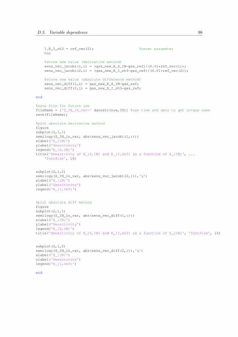
D.5. Variable dependence 98
l.K_I_nh3 = ref_vec(2); %reset parametertoc
%store new value (derivative method)sens_vec_jacobi(1,i) = (gas_new_K_S_IN−gas_ref)/(0.01*ref_vec(1));sens_vec_jacobi(2,i) = (gas_new_K_I_nh3−gas_ref)/(0.01*ref_vec(2));
%store new value (absolute difference method)sens_vec_diff(1,i) = gas_new_K_S_IN−gas_ref;sens_vec_diff(2,i) = gas_new_K_I_nh3−gas_ref;
end
%save file for future usefileName = ['S_IN_in_var−' datestr(now,30)] %use time and date to get unique namesave(fileName);
%plot absolute derivative methodfiguresubplot(2,1,1)semilogy(S_IN_in_var, abs(sens_vec_jacobi(1,:)))xlabel('S_{IN}')ylabel('Sensitivity')legend('K_{S,IN}')title('Sensitivity of K_{S,IN} and K_{I,nh3} as a function of S_{IN}', ...
'fontSize', 16)
subplot(2,1,2)semilogy(S_IN_in_var, abs(sens_vec_jacobi(2,:)),'g')xlabel('S_{IN}')ylabel('Sensitivity')legend('K_{I,nh3}')
%plot absolute diff methodfiguresubplot(2,1,1)semilogy(S_IN_in_var, abs(sens_vec_diff(1,:)))xlabel('S_{IN}')ylabel('Sensitivity')legend('K_{S,IN}')title('Sensitivity of K_{S,IN} and K_{I,nh3} as a function of S_{IN}', 'fontSize', 16)
subplot(2,1,2)semilogy(S_IN_in_var, abs(sens_vec_diff(2,:)),'g')xlabel('S_{IN}')ylabel('Sensitivity')legend('K_{I,nh3}')
end

D.5. Variable dependence 99
%function for calculating gas production when the process has reached a%steady statefunction mean_gas = calculate_mean_gas(l,y0)%settings for ODE−solveroptions = odeset('RelTol', 1e−10, 'AbsTol', 1e−10);
%solve ADM1 problem[T,solution] = ode15s(@(t,y) ADM1_fun_v2_ODE(t,y,l), [0 200],y0, options);
%retrive gas concentrationS_gas_h2 = solution(:,33);S_gas_ch4 = solution(:,34);S_gas_co2 = solution(:,35);
%calculate gas pressureP_gas_h2 = S_gas_h2*l.R*l.T_op/16;P_gas_ch4 = S_gas_ch4*l.R*l.T_op/64;P_gas_co2 = S_gas_co2*l.R*l.T_op;
P_gas = P_gas_h2+P_gas_ch4+P_gas_co2+l.p_gas_h2o; %total gas pressureq_gas = l.k_p*(P_gas−l.P_atm).*P_gas/l.P_atm; %total gas flow
q_gas_ch4 = P_gas_ch4./P_gas.*q_gas; %CH4 gas flowmean_gas = mean(q_gas_ch4(end−100:end)); %mean gas production at steady stateend

D.6
Part
icle
Sw
arm
op
tim
izati
on
%MasterThesis
% %AppliedPhysics
%ChalmersUniversityofTechnolopgy
%Spring2014
% %OskarDanielsson
% %FileforrunningaParticleSwarmOptimization(PSO)methodinorderto
%findmaximumgaspossibiltoproduceoutofcodigestingbetweenmanure
%andwastewater.
% %Theimplementationfollowsthebook"Biologicallyinspiredoptimization
%methods"byWahde,Mattias
% %Bychancingtheintervallscalledlimitsbelowthepossibleintervallsin
%whichthesolutionlivescanbedetermined.Ifonewantstohaveafixed
%valueforoneormoreofthosequantitieschosingupperandlowerlimits
%equalwillfixthis.
functionOneFilePSO_vector_report
addpath('../ADM1');
%defineparametersforoptimization
%..........................................................................
%definelimitsinwhichthesolutionlives
limits
=[0.01,
0.01;
...S_su_min,
S_su_max
0.001,0.001;...S_aa_min,
S_aa_max
0.001,0.001;...S_fa_min,
S_fa_max
0.001,0.001;...S_va_min,
S_va_max
0.001,0.001;...S_bu_min,
S_bu_max
0.001,0.001;...S_pro_min,S_pro_max
0.001,0.001;...S_ac_min,
S_ac_max

1e−8,
1e−8;
...S_h2_min,
S_h2_max
1e−5,
1e−5;
...S_ch4_min,S_ch4_max
0,
1;
...S_IC_min,
S_IC_max
0,
1;
...S_IN_min,
S_IN_max
0.02,
0.02;
...S_I_min,
S_I_max
%......................................
2,
2;
...X_xc_min,
X_xc_max
5,
5;
...X_ch_min,
X_ch_max
20,
20;
...X_pr_min,
X_pr_max
5,
5;
...X_li_min,
X_li_max
0,
0;
...X_su_min,
X_su_max
0.01,
0.01;
...X_aa_min,
X_aa_max
0.01,
0.01;
...X_fa_min,
X_fa_max
0.01,
0.01;
...X_c4_min,
X_c4_max
0.01,
0.01;
...X_pro_min,X_pro_max
0.01,
0.01;
...X_ac_min,
X_ac_max
0.01,
0.01;
...X_h2_min,
X_h2_max
25,
25;
...X_I_min,
X_I_max
%......................................
0.04,
0.04;
...S_cat_min,X_cat_max
0.02,
0.02;
...S_an_min,
X_an_max
%......................................
100,
200;
...q_min,
q_max
%......................................
0,
0;
...S_lac_min,S_lac_max
0,
0;
...X_lac_f_min,X_lac_f_max
0,
0;
...X_lac_o_min,X_lac_o_max
0,
0;
...S_ca_min,
S_ca_max
%......................................
];
nParticles
=20;
%numberofparticlesinPSO
alpha
=1;
%PSOconstant
c1
=2;
%PSOconstant
c2
=2;
%PSOconstant
limit
=1000;%numberofiterations
%chosingmaximumspeedforeachdimensiontoatenthofitsrange
vmax=abs((limits(:,2)−limits(:,1))/10);

%initializeparticles
particles=InitializeParticles(nParticles,alpha,limits);
iIterations=0;%numberofiterationsdone
bestGlobalFunctionValue=inf;%givealargestartvaluetouserealvaluesinsimulation
bestGlobalPosition=zeros(size(limits,1),1);%definevariableforbestglobalposition
%doactualoptimizationloop
whileiIterations<limit
iIterations=iIterations+1;
%foreachparticleinswarm
fori=1:nParticles
currentParticle=particles(i);
currentFunctionValue=FunctionToMinimize(currentParticle);
%testifcurrentvalueisglobaland/orparticlebest
[bestGlobalFunctionValue,bestGlobalPosition]=...
UpdateGlobalBest(currentParticle,currentFunctionValue,...
bestGlobalFunctionValue,bestGlobalPosition);
currentParticle=UpdateParticleBest(currentParticle,currentFunctionValue);
particles(i)=currentParticle;
end
%updateallswarmparticlesstates
fori=1:nParticles
particles(i)=UpdateParticleState(particles(i),c1,c2,vmax,...
bestGlobalPosition,limits);
end
end%mainwhileloop
end%mainfunction
%functionforinitializingparticles
functionparticles=InitializeParticles(nParticles,alpha,limits)

%initializeallparticles
fori=1:nParticles
particle=struct;%definingastructthatwillbetheparticle
%definefieldsinthestructtostoredata
particle.position
=zeros(size(limits,1),1);
particle.velocity
=zeros(size(limits,1),1);
particle.bestLocalPosition=zeros(size(limits,1),1);
%Positions(atstartthefirstpositionistheknownbest)
forj=1:size(limits,1)
r=rand;
particle.position(j)=limits(j,1)+r*(limits(j,2)−limits(j,1));
particle.bestLocalPosition(j)=particle.position(j);
end
%functionvalues,setonlyknownasfunctionbest
particle.fb=FunctionToMinimize(particle);
%defineparticlevelocity
forj=1:size(limits,1)
r=rand;
particle.velocity(j)=alpha*(−(limits(j,2)−limits(j,1))/...
2+r*(limits(j,2)−limits(j,1)));
end
particles(i)=particle;%savecurrentparticletovectorofparticles
end%initializeloop
end%initializefunction
%functionforcalculatingparticlesfunctionvalue
function[mean_gas]=FunctionToMinimize(particle)
l=IndataADM1_v2;%readindatafromfile
%changetocorrectvaluesofvariables(fromstandardinputtocurrentvalue)
l.S_su_in
=particle.position(1);
l.S_aa_in
=particle.position(2);
l.S_fa_in
=particle.position(3);

l.S_va_in
=particle.position(4);
l.S_bu_in
=particle.position(5);
l.S_pro_in
=particle.position(6);
l.S_ac_in
=particle.position(7);
l.S_h2_in
=particle.position(8);
l.S_ch4_in
=particle.position(9);
l.S_IC_in
=particle.position(10);
l.S_IN_in
=particle.position(11);
l.S_I_in
=particle.position(12);
l.X_xc_in
=particle.position(13);
l.X_ch_in
=particle.position(14);
l.X_pr_in
=particle.position(15);
l.X_li_in
=particle.position(16);
l.X_su_in
=particle.position(17);
l.X_aa_in
=particle.position(18);
l.X_fa_in
=particle.position(19);
l.X_c4_in
=particle.position(20);
l.X_pro_in
=particle.position(21);
l.X_ac_in
=particle.position(22);
l.X_h2_in
=particle.position(23);
l.X_I_in
=particle.position(24);
l.S_cat_in
=particle.position(25);
l.S_an_in
=particle.position(26);
l.q_in
=particle.position(27);
l.S_lac_in
=particle.position(28);
l.X_lac_f_in=particle.position(29);
l.X_lac_o_in=particle.position(30);
l.S_ca_in
=particle.position(31);
%startvaluesforsimulation
y0=[0.009;...
%S_su
0.0009;...
%S_aa
0.0009;...
%S_fa
0.0009;...
%S_va
0.0009;...
%S_bu
0.0009;...
%S_pro
0.0009;...
%S_ac
2.3594e−9;...%S_h2

2.3594e−6;...%S_ch4
0.039;...
%S_IC
0.13023;...
%S_IN
0.009;...
%S_I
0.30870;...
%X_c
0.02795;...
%X_ch
0.10260;...
%X_pr
0.02948;...%X_li
0.42016;...
%X_su
1.17917;...
%X_aa
0.24303;...
%X_fa
0.43192;...
%X_c4
0.13730;...
%X_pro
0.76056;...
%X_ac
0.31702;...
%X_h2
25.61739;...%X_I
0.04;...
%S_cat
0.02;...
%S_an
0.0116;...
%S_vam
0.01322;...
%S_bum
0.01574;...
%S_prom
0.19724;...
%S_acm
0.14278;...
%S_hco3m
0.00409;...
%S_nh3
1.023e−5;...%h2
1.62125;...
%ch4
0.01411;...
%co2
0;...
%S_lac
0;...
%X_lac_f
0;...
%X_lac_o
0];
%S_ca
%doactualcalculation
options=odeset('RelTol',1e−10,'AbsTol',1e−10);
[T,solution]=ode15s(@(t,y)ADM1_fun_v2_ODE(t,y,l),[050],y0,options);

S_gas_h2
=solution(:,33);
S_gas_ch4=solution(:,34);
S_gas_co2=solution(:,35);
P_gas_h2
=S_gas_h2*l.R*l.T_op/16;
P_gas_ch4=S_gas_ch4*l.R*l.T_op/64;
P_gas_co2=S_gas_co2*l.R*l.T_op;
P_gas=P_gas_h2+P_gas_ch4+P_gas_co2+l.p_gas_h2o;%totalgaspressure
q_gas
=l.k_p*(P_gas−l.P_atm).*P_gas/l.P_atm;%totalgasflow
q_gas_ch4=P_gas_ch4./P_gas.*q_gas;
mean_gas=mean(q_gas_ch4(end−100:end));
mean_gas=−mean_gas;%tofindmaximuminsteadofminimum
end%functionvaluecalculator
%functionforupadateglobalbestiftheparticlespositionisglobalbest
function[bestGlobalFunctionValue,bestGlobalPosition]=...
UpdateGlobalBest(currentParticle,candidateFunctionValue,...
bestGlobalFunctionValue,bestGlobalPosition)
%ifcadidatevaluearebetterchange
if(candidateFunctionValue<bestGlobalFunctionValue)
bestGlobalFunctionValue=candidateFunctionValue;
bestGlobalPosition=currentParticle.position;
fprintf('NewbestPositionfound:\n−−−−−−−−−−−−−−−−−−−−−
\nS_su=%.4f\nS_aa=%.4f\nS_fa=%.4f
\nS_va=%.4f\nS_bu=%.4f\nS_pro=%.4f\nS_ac=%.4f\nS_h2=%.4f\nS_ch4=%.4f\nS_IC=%.4f\nS_IN=%.4f
\nS_I=%.4f\nX_xc=%.4f\nX_ch=%.4f\nX_pr=%.4f\nX_li=%.4f\nX_su=%.4f\nX_aa=%.4f\nX_fa=%.4f
\nX_c4=%.4f\nX_pro=%.4f\nX_ac=%.4f\nX_h2=%.4f\nX_I=%.4f\nS_cat=%.4f\nS_an=%.4f\nq=%.4f
\nS_lac=%.4f\nX_lac_f=%.4f\nX_lac_o=%.4f\nS_ca=%.4f\n−−−−−−−−−−−−−−−−−−−−−
\nf=%.8f\n=====================\n',...
bestGlobalPosition(1),
bestGlobalPosition(2),
bestGlobalPosition(3),...
bestGlobalPosition(4),
bestGlobalPosition(5),
bestGlobalPosition(6),...
bestGlobalPosition(7),
bestGlobalPosition(8),
bestGlobalPosition(9),...
bestGlobalPosition(10),bestGlobalPosition(11),bestGlobalPosition(12),...

bestGlobalPosition(13),bestGlobalPosition(14),bestGlobalPosition(15),...
bestGlobalPosition(16),bestGlobalPosition(17),bestGlobalPosition(18),...
bestGlobalPosition(19),bestGlobalPosition(20),bestGlobalPosition(21),...
bestGlobalPosition(22),bestGlobalPosition(23),bestGlobalPosition(24),...
bestGlobalPosition(25),bestGlobalPosition(26),bestGlobalPosition(27),...
bestGlobalPosition(28),bestGlobalPosition(29),bestGlobalPosition(30),...
bestGlobalPosition(31),−bestGlobalFunctionValue);
%addminussigntocompensatetodisplaycorrectvalue.Function
%calculationgivesminusforplusandviceverca.
end%if
end%UpdateGlobalBest
%functionforupdatingtheparticlebestifitisso
functioncurrentParticle=UpdateParticleBest(currentParticle,candidateFunctionValue)
%ifcurrentvalueisbetterthatbestknownbest,changelocalbest
if(candidateFunctionValue<currentParticle.fb)
currentParticle.fb=candidateFunctionValue;
currentParticle.bestLocalPosition=currentParticle.position;
end%if
end%currentParticle
%functionformovingtheparticleandupdateitsstates
%keepstrackofmovingtheparticleinsidetheboundaries
functionparticle=UpdateParticleState(particle,c1,c2,vmax,bestGlobalPosition,limits)
%update
velocitiesandpositions(butcheckifboudariesarefullfilled)
fori=1:size(limits,1)
%findtorandomnumberstobeusedinupdatingnewvelocity
q=rand();
r=rand();
particle.velocity(i)=c1*q*(particle.bestLocalPosition(i)−
particle.position(i))+...
c2*r*(bestGlobalPosition(i)−
particle.position(i));

%setthevelocitytobeinallowedregion
particle.velocity(i)=min(particle.velocity(i),vmax(i));
particle.velocity(i)=max(particle.velocity(i),−vmax(i));
%settingnewposition
particle.position(i)=particle.position(i)+particle.velocity(i);
%takecareofboundaries
if(particle.position(i)<limits(i,1))
particle.position(i)=limits(i,1);
elseif(particle.position(i)>limits(i,2))
particle.position(i)=limits(i,2);
end
end
end%UpdateParticleState

D.7. GUI 109
D.7 GUI
D.7.1 Run GUI (mac)
%Master Thesis%%Applied Physics%Chalmers University of Technolopgy%Spring 2014%%Oskar Danielsson%[email protected]%%Main function for running the GUI on mac%
function RunGUIMacGUI_ADM1;end

D.7. GUI 110
D.7.2 Run GUI (Windows)
%Master Thesis%%Applied Physics%Chalmers University of Technolopgy%Spring 2014%%Oskar Danielsson%[email protected]%%Main function for running the GUI on Windows. Due to problems (chnages) in%centimeter definitions between mac and Windows are positions redefined in%GUI to work in an Windows environment. Everything else is kept.%
%run gui, and get access to all graphical objects to set their psitionsgo = GUI_ADM1;
%meassure screen height to fit everything it the displayable areascreenHeight = get(0, 'screenSize')/get(0, 'ScreenPixelsPerInch')*2.54;screenHeight = screenHeight(4); %height of screen
%screenHeight = 15; %use this to simulate smaller scree
%define figure (window) for perfect conditionswindowHeight = 24; %main fig window heightinTableHeight = 14.9; %in table heightinTableTextPos = 22.6; %text position on top of in tablestartTableHeight = 18.6; %start table heightstartTableTextPos = 22.6; %text position on top of start table
%redefine positions and heights if not fitted in viewable areaif(screenHeight − 2 < windowHeight)
windowHeight = screenHeight−2;inTableHeight = windowHeight − 7.7 − 1;inTableTextPos = inTableHeight + 7.7;startTableHeight = windowHeight − 4 − 1;startTableTextPos = startTableHeight + 4;
end
%settings for main window and its input componentsset(go.mainFigHandle, 'position', [10, 2, 23.5, windowHeight])set(go.handleInTable, 'position', [1 7.7 7 inTableHeight])set(go.inTableText, 'position', [1 inTableTextPos 7 .8])set(go.handleStartTable, 'position', [9 4 7.1 startTableHeight])set(go.startTableText, 'position', [9 startTableTextPos 7.1 .8])
%settings for plot selections

D.7. GUI 111
boxGroupHeight = 18.6;
if(boxGroupHeight > windowHeight)boxGroupHeight = startTableHeight;
end
set(go.handleBoxGroup, 'position', [17.1 4 5.2 boxGroupHeight]);for i = 1:length(go.handleCheckBoxes)
if(i<25)set(go.handleCheckBoxes(i), 'position', [0.1, boxGroupHeight−...
(boxGroupHeight/(length(go.handleCheckBoxes))*2)*i, 2.5, .4]);else
set(go.handleCheckBoxes(i), 'position', [2.6, boxGroupHeight−...(boxGroupHeight/(length(go.handleCheckBoxes))*2)*(i−24), 2.2, .4]);
endendset(go.plotSelectionText, 'position', [17.1 4+boxGroupHeight, 5.2 .8])
%settings for parameter figuresset(go.handleFlowField, 'position', [3 6 3 1])set(go.flowFieldText, 'position', [.5 6 2 .8])set(go.handleTimeField, 'position', [3 4.5 3 1])set(go.timeFieldText, 'position', [.5 4.5 2 .8])
set(go.handleParamTable(1), 'position', [1 1 7.8 15])set(go.handleParamTable(1), 'columnWidth', {'auto', 110})set(go.paramFigHandle(1), 'position', [2 2 9.8 17.5])set(go.paramFigText(1), 'position', [1 16 7.8 .8])
set(go.handleParamTable(2), 'position', [1 1 6.7 12])set(go.paramFigText(2), 'position', [1 13 6.7 .8])set(go.paramFigHandle(2), 'position', [2 2 8.7 14.5])
set(go.handleParamTable(3), 'position', [1 1 6.1 1.6])set(go.paramFigText(3), 'position', [1 2.6 6.1 .8])set(go.paramFigHandle(3), 'position', [2 2 8.1 4])
set(go.handleParamTable(4), 'position', [1 1 8.3 15])set(go.paramFigText(4), 'position', [1 16 8.3 .8])set(go.paramFigHandle(4), 'position', [2 2 10.3 17.3])

D.7. GUI 112
D.7.3 Main GUI
%Master Thesis%%Applied Physics%Chalmers University of Technolopgy%Spring 2014%%Oskar Danielsson%[email protected]%%File for runnig the implemented ADM1 model without using the coding%environment of MATLAB. The source code below can be compiled to an stand%alone executable that can be used by persons lacking access to MATLAB.%
function [graphicalObjects] = GUI_ADM1
addpath('../ADM1')
%read this to fill fieldsl = IndataADM1_v2;l.time = 50; %chose default simulation time to be 50
hf = figure; %handle to main window
%declare figures for edit parameter valueshf_Param(1) = figure;set(hf_Param(1), ...
'Name', 'Stoichiometric parameter values', ...'NumberTitle', 'off', ...'MenuBar', 'none', ...'visible', 'off', ...'Units', 'centimeters', ...'Position', [1 1 12.5 30], ...'CloseRequestFcn', @Close_cb);
hf_Param(2) = figure;set(hf_Param(2), ...
'Name', 'Physicochemical parameter values', ...'NumberTitle', 'off', ...'MenuBar', 'none', ...'visible', 'off', ...'Units', 'centimeters', ...'Position', [1 1 11.6 18], ...'CloseRequestFcn', @Close_cb);
hf_Param(3) = figure;set(hf_Param(3), ...
'Name', 'Physical parameter values', ...'NumberTitle', 'off', ...

D.7. GUI 113
'MenuBar', 'none', ...'visible', 'on', ...'Units', 'centimeters', ...'Position', [1 1 10.8 5], ...'CloseRequestFcn', @Close_cb);
hf_Param(4) = figure;set(hf_Param(4), ...
'Name', 'Biochemcial parameter values', ...'NumberTitle', 'off', ...'MenuBar', 'none', ...'visible', 'off', ...'Units', 'centimeters', ...'Position', [1 1 13 30], ...'CloseRequestFcn', @Close_cb);
%basic settings for current created figureset(hf, ...
'Name', 'ADM1 − GUI', ...'NumberTitle', 'off', ...'MenuBar', 'none', ...'Units', 'Centimeters', ...'Position', [10, 1, 26.5, 29.5], ...'Resize', 'off', ...'CloseRequestFcn', {@CloseMainFig,hf_Param});
%==================================================================%% Define graphical objects%%==================================================================
%fill parameter tables with data[paramStoioTableData, paramStoioTableRowNames, paramStoioTableColumnName] = ...
FillStoichiometricTable(l);figure(hf_Param(1))handleParamTable(1) = uitable(...
'Units', 'Centimeters', ...'Position', [ 1.5 1 9.5 27.2],...'Data', paramStoioTableData, ...'rowName', paramStoioTableRowNames, ...'ColumnName', paramStoioTableColumnName,...'ColumnWidth', {'auto', 110}, ...'ColumnEditable', [true, false]);
paramFigText(1) = uicontrol(...'Style', 'text', ...'Units', 'Centimeters', ...'Position', [1.5 28.5 8.3 .8], ...'String', 'Stoichiometric parameter values', ...'BackgroundColor', [.8 .8 .8]);
set(hf_Param(1), 'visible', 'off')
[paramPhysicochemicalTableData, paramPhysicochemicalTableRowNames, ...

D.7. GUI 114
paramPhysicochemicalTableColumnName] = FillPhysicochemicalTable(l);figure(hf_Param(2))handleParamTable(2) = uitable(...
'Units', 'Centimeters', ...'Position', [ 1.5 1 8.6 15.2],...'Data', paramPhysicochemicalTableData, ...'rowName', paramPhysicochemicalTableRowNames, ...'ColumnName', paramPhysicochemicalTableColumnName,...'ColumnEditable', [true, false]);
paramFigText(2) = uicontrol(...'Style', 'text', ...'Units', 'Centimeters', ...'Position', [1.5 16.5 8.6 .8], ...'String', 'Physicochemical parameter values', ...'BackgroundColor', [.8 .8 .8]);
set(hf_Param(2), 'visible', 'off')
[paramPhysicaclTableData, paramPhysicalTableRowNames, ...paramPhysicalTableColumnName] = FillPhysicalTable(l);
figure(hf_Param(3))handleParamTable(3) = uitable(...
'Units', 'Centimeters', ...'Position', [ 1.5 1 7.9 2],...'Data', paramPhysicaclTableData, ...'rowName', paramPhysicalTableRowNames, ...'ColumnName', paramPhysicalTableColumnName,...'ColumnEditable', [true, false]);
paramFigText(3) = uicontrol(...'Style', 'text', ...'Units', 'Centimeters', ...'Position', [1.5 3.5 7.9 .8], ...'String', 'Physicochemical parameter values', ...'BackgroundColor', [.8 .8 .8]);
set(hf_Param(3), 'visible', 'off')
[paramBiochemicalTableData, paramBiochemicalTableRowNames, ...paramBiochemicalTableColumnName] = FillBiochemicalTable(l);
figure(hf_Param(4))handleParamTable(4) = uitable(...
'Units', 'Centimeters', ...'Position', [ 1.5 0.5 10 28.5],...'Data', paramBiochemicalTableData, ...'rowName', paramBiochemicalTableRowNames, ...'ColumnName', paramBiochemicalTableColumnName,...'ColumnEditable', [true, false]);
paramFigText(4) = uicontrol(...'Style', 'text', ...'Units', 'Centimeters', ...'Position', [1.5 29 10 .8], ......'String', 'Biochemical parameter values', ...'BackgroundColor', [.8 .8 .8]);
set(hf_Param(4), 'visible', 'off')

D.7. GUI 115
%select correct figure to place all components infigure(hf)
%declare a table with all input flows[inTableData, inTableRowNames, inTableColumnName] = FillInTable(l);handleInTable = uitable(...
'Units', 'Centimeters', ...'Position', [ 1 9.7 9 18.8],...'Data', inTableData, ...'rowName', inTableRowNames, ...'ColumnName', inTableColumnName,...'ColumnEditable', [true, false]);
inTableText = uicontrol(...'Style', 'text', ...'Units', 'Centimeters', ...'Position', [1 28.5 9 .8], ...'String', 'Inflow', ...'FontSize', 14, ...'BackgroundColor', [.8 .8 .8]);
%declare a table with starting values[startTabledata, startTableRowNames, startTableColumnName] = FillStartTable;handleStartTable = uitable(...
'Units', 'Centimeters', ...'Position', [ 11 4.35 8.6 24.15],...'Data', startTabledata, ...'rowName', startTableRowNames, ...'ColumnName', startTableColumnName,...'ColumnEditable', [true, false]);
startTableText = uicontrol(...'Style', 'text', ...'Units', 'Centimeters', ...'Position', [10.5 28.5 8.6 .8], ...'String', 'Start values', ...'FontSize', 14, ...'BackgroundColor', [.8 .8 .8]);
%define checkboxes for chosing plots from modelnameString = {'S_su', 'S_aa', 'S_fa', 'S_va', ...
'S_bu', 'S_pro', 'S_ac', 'S_h2', 'S_ch4',...'S_IC', 'S_IN', 'S_I', 'X_xc', 'X_ch', ...'X_pr', 'X_li', 'X_su', 'X_aa', 'X_fa', ...'X_c4', 'X_pro', 'X_ac', 'X_h2', 'X_I', ...'S_cat', 'S_an', 'pH', ...'S_H+', 'S_va−', 'S_bu−', 'S_pro−', ...'S_ac−', 'S_hco3−', 'S_co2', 'S_nh3', ...'S_nh4+', 'S_gas,h2', 'S_gas,ch4', 'S_gas,co2', ...'p_gas,h2', 'p_gas,ch4', 'p_gas,co2', 'p_gas', ...'q_gas', 'S_lac', 'X_lac,f', 'X_lac,o', ...'S_ca'};

D.7. GUI 116
boxGroupHeight = 27.5;handleBoxGroup = uibuttongroup('visible','off', 'Units', 'Centimeters', ...
'Position', [20.5 1 5 boxGroupHeight]);for i = 1:length(nameString)
h_B(i) = uicontrol(...'Style', 'checkbox', ...'String', nameString(i), ...'Units', 'Centimeters', ...'Position', [0.1, boxGroupHeight−(boxGroupHeight/length(nameString))*...
i, 4, .5], ...'Parent', handleBoxGroup, ...'HandleVisibility','off');
%define callback under definition for run buttonendset(handleBoxGroup,'SelectedObject',[]); % No selectionset(handleBoxGroup,'Visible','on');plotSelectionText = uicontrol(...
'Style', 'text',...'Units', 'Centimeters', ...'Position',[20.5 28.5 5 .8], ...'String', 'Plot selection', ...'FontSize', 14, ...'BackgroundColor', [.8 .8 .8]);
%declare a flow fieldhandleFlowField = uicontrol(...
'Style', 'edit', ...'Units', 'Centimeters',...'Position', [3 7 3 1],...'Backgroundcolor', [1 1 1], ...'String', num2str(l.q_in));
flowFieldText = uicontrol(...'Style', 'text', ...'Units', 'Centimeters', ...'Position', [.5 7 2 .8], ...'String', 'Flow', ...'FontSize', 14, ...'BackgroundColor', [.8 .8 .8]);
%declare a integration time fieldhandleTimeField = uicontrol(...
'Style', 'edit',...'Units', 'Centimeters', ...'Position', [3 5 3 1], ...'Backgroundcolor', [1 1 1], ...'String', num2str(l.time));
timeFieldText = uicontrol(...'Style', 'text', ...'Units', 'Centimeters', ...'Position', [.5 5 2 .8], ...'String', 'Time', ...

D.7. GUI 117
'FontSize', 14, ...'BackgroundColor', [.8 .8 .8]);
%declare a run buttonleftPos = 12; %position for most left button in grouphandleRunButton = uicontrol(...
'Style', 'PushButton',...'Units', 'Centimeters',...'Position', [leftPos+4 1.5 2 1],...'String', 'Run', ...'Enable', 'off', ...'Callback', {@Run_cb,handleInTable,handleFlowField,handleTimeField,...handleStartTable, h_B, handleParamTable});
set(h_B, 'Callback', {@Check_cb, handleRunButton, h_B});
handleSaveButton = uicontrol(...'Style', 'PushButton',...'Units', 'Centimeters',...'Position', [leftPos+2 1.5 2 1],...'String', 'Save', ...'Callback', {@Save_cb,handleInTable,handleFlowField,handleTimeField,...handleStartTable, handleParamTable});
handleLoadButton = uicontrol(...'Style', 'PushButton',...'Units', 'Centimeters',...'Position', [leftPos 1.5 2 1],...'String', 'Load', ...'Callback', {@Load_cb,handleInTable,handleFlowField,handleTimeField,...handleStartTable, handleParamTable});
%declare buttons for chanching parameter valuesparamButton(1) = uicontrol(...
'Style', 'PushButton',...'Units', 'Centimeters',...'Position', [1 1 4 1],...'String', 'Stoichiometric', ...'Tag', '1', ...'Callback', {@EditParameters_cb, hf_Param});
paramButton(2) = uicontrol(...'Style', 'PushButton',...'Units', 'Centimeters',...'Position', [1 2 4 1],...'String', 'Physicochemical', ...'Tag', '2', ...'Callback', {@EditParameters_cb, hf_Param});
paramButton(3) = uicontrol(...'Style', 'PushButton',...'Units', 'Centimeters',...'Position', [5 1 4 1],...'String', 'Physical', ...

D.7. GUI 118
'Tag', '3', ...'Callback', {@EditParameters_cb, hf_Param});
paramButton(4) = uicontrol(...'Style', 'PushButton',...'Units', 'Centimeters',...'Position', [5 2 4 1],...'String', 'Biochemical', ...'Tag', '4', ...'Callback', {@EditParameters_cb, hf_Param});
paramText = uicontrol(...'Style', 'text',...'Units', 'Centimeters', ...'Position',[1 3 8 .8], ...'String', 'Edit Parameter Values', ...'FontSize', 14, ...'BackgroundColor', [.8 .8 .8]);
%create a struct with all handles to be used when setting sizes of objects%in a Windows environmentgraphicalObjects = struct();graphicalObjects.parmButton = paramButton;graphicalObjects.paramText = paramText;graphicalObjects.loadButton = handleLoadButton;graphicalObjects.saveButton = handleSaveButton;graphicalObjects.runButton = handleRunButton;graphicalObjects.timeFieldText = timeFieldText;graphicalObjects.handleTimeField = handleTimeField;graphicalObjects.flowFieldText = flowFieldText;graphicalObjects.handleFlowField = handleFlowField;graphicalObjects.plotSelectionText = plotSelectionText;graphicalObjects.handleCheckBoxes = h_B;graphicalObjects.handleBoxGroup = handleBoxGroup;graphicalObjects.inTableText = inTableText;graphicalObjects.handleInTable = handleInTable;graphicalObjects.startTableText = startTableText;graphicalObjects.handleStartTable = handleStartTable;graphicalObjects.handleParamTable = handleParamTable;graphicalObjects.paramFigText = paramFigText;graphicalObjects.mainFigHandle = hf;graphicalObjects.paramFigHandle = hf_Param;end
%..........................................................................%main execution buttons (load, save and run)%..........................................................................
%function that loads saved values from an old runfunction Load_cb(handle, event, handleInTable,handleFlowField,...
handleTimeField,handleStartTable, handleParamTable)[file_name, path_to_file] = uigetfile('*.mat', 'title')

D.7. GUI 119
%if cancle do nothingif(file_name == 0)
returnend
%load fileload([path_to_file file_name]);
%update all data fields to the loaded valuesset(handleInTable, 'Data', inData);set(handleFlowField, 'String', num2str(flowData))set(handleTimeField, 'String', num2str(timeData))set(handleStartTable, 'Data', startData);set(handleParamTable(1), 'Data', stoichiometricData);set(handleParamTable(2), 'Data', physiochemicalData);set(handleParamTable(3), 'Data', physicalData);set(handleParamTable(4), 'Data', biochemicalData);end
%funcctiond that save states for future usefunction Save_cb(handle, event, handleInTable,handleFlowField,...
handleTimeField,handleStartTable, handleParamTable)%read and data from all fieldsinData = get(handleInTable, 'Data');flowData = str2double(get(handleFlowField,'String'));timeData = str2double(get(handleTimeField,'String'));startData = get(handleStartTable, 'Data');stoichiometricData = get(handleParamTable(1),'Data');physiochemicalData = get(handleParamTable(2), 'Data');physicalData = get(handleParamTable(3), 'Data');biochemicalData = get(handleParamTable(4), 'Data');
%save the data with a specific file name (chosen at execution time)uisave({'inData', 'flowData', 'timeData', 'startData', ...
'stoichiometricData', 'physiochemicalData', 'physicalData', ...'biochemicalData'},'unitled');
end
%calback for run buttonfunction Run_cb(handle, event, handleInTable, handleFlowField, ...
handleTimeField, handleStartTable, handleCheckedPlot, handleParamTable)%read updated indata from parameters from file, table and flow fieldset(handle,'enable', 'off') %prevent user from starting a new simulation
%while one is runningdrawnow[l, y0] = Update_values(handleInTable, handleFlowField, handleTimeField, ...
handleStartTable, handleParamTable);
%solve ADM1 system of ODEsoptions = odeset('RelTol', 1e−10, 'AbsTol', 1e−10);[T,solution] = ode15s(@(t,y) ADM1_fun_v2_ODE(t,y,l), [0 l.time],y0, options);
%retrive and store solution in result struct * r *

D.7. GUI 120
r.S_su = solution(:,1);r.S_aa = solution(:,2);r.S_fa = solution(:,3);r.S_va = solution(:,4);r.S_bu = solution(:,5);r.S_pro = solution(:,6);r.S_ac = solution(:,7);r.S_h2 = solution(:,8);r.S_ch4 = solution(:,9);r.S_IC = solution(:,10);r.S_IN = solution(:,11);r.S_I = solution(:,12);r.X_c = solution(:,13);r.X_ch = solution(:,14);r.X_pr = solution(:,15);r.X_li = solution(:,16);r.X_su = solution(:,17);r.X_aa = solution(:,18);r.X_fa = solution(:,19);r.X_c4 = solution(:,20);r.X_pro = solution(:,21);r.X_ac = solution(:,22);r.X_h2 = solution(:,23);r.X_I = solution(:,24);r.S_cat = solution(:,25);r.S_an = solution(:,26);r.S_vam = solution(:,27);r.S_bum = solution(:,28);r.S_prom = solution(:,29);r.S_acm = solution(:,30);r.S_hco3m = solution(:,31);r.S_nh3 = solution(:,32);r.S_gas_h2 = solution(:,33);r.S_gas_ch4 = solution(:,34);r.S_gas_co2 = solution(:,35);r.S_lac = solution(:,36);r.X_lac_f = solution(:,37);r.X_lac_o = solution(:,38);r.S_ca = solution(:,39);
r.T = T; %save simulation time
%calculate pressurer.P_gas_h2 = r.S_gas_h2*l.R*l.T_op/16;r.P_gas_ch4 = r.S_gas_ch4*l.R*l.T_op/64;r.P_gas_co2 = r.S_gas_co2*l.R*l.T_op;
%call function to plot wanted resultPlotGUIResult(l, r, handleCheckedPlot, solution);
%make it possible to run simulation againset(handle, 'enable', 'on')end

D.7. GUI 121
%calback for check boxes that activates Run button when any plot is%selectedfunction Check_cb(handle, event, handleRunButton, h_B)%if box is selected enable Run and return else test if there is an other%box checkedif(get(handle, 'Value'))
set(handleRunButton, 'enable', 'on')return
else%see if any box is still checked if so do nothing, else disable RunnumPlots = 0;for i = 1:length(h_B)
if(get(h_B(i), 'Value'))numPlots = numPlots + 1;continue
endendif(numPlots == 0)
set(handleRunButton, 'enable', 'off');end
endend
%..........................................................................%fill (at start of program) and view parameter tables%..........................................................................
%function for filling biochemical parameter tablefunction [data, rowNames, columnName] = FillBiochemicalTable(l)%read data from ldata = {...
l.k_dis, ' d^−1';l.k_hyd_ch, ' d^−1';l.k_hyd_pr, ' d^−1';l.k_hyd_li, ' d^−1';l.K_S_IN, ' M';l.k_m_su, ' d^−1';l.K_S_su, ' kg COD m^−3';l.pH_UL_aa, ' −';l.pH_LL_aa, ' −';l.k_m_aa, ' d^−1';l.K_S_aa, ' kg COD m^−3';l.k_m_fa, ' d^−1';l.K_S_fa, ' kg COD m^−3';l.K_I_h2_fa, ' kg COD m^−3';l.k_m_c4, ' d^−1';l.K_S_c4, ' kg COD m^−3';l.K_I_h2_c4, ' kg COD m^−3';l.k_m_pro, ' d^−1';l.K_S_pro, ' kg COD m^−3';l.K_I_h2_pro, ' kg COD m^−3';

D.7. GUI 122
l.k_m_ac, ' d^−1';l.K_S_ac, ' kg COD m^−3';l.K_I_nh3, ' kg COD m^−3';l.pH_UL_ac, ' −';l.pH_LL_ac, ' −';l.k_m_h2, ' d^−1';l.K_S_h2, ' kg COD m^−3';l.pH_UL_h2, ' −';l.pH_LL_h2, ' −';l.k_dec_X_su, ' d^−1';l.k_dec_X_aa, ' d^−1';l.k_dec_X_fa, ' d^−1';l.k_dec_X_c4, ' d^−1';l.k_dec_X_pro, ' d^−1';l.k_dec_X_ac, ' d^−1';l.k_dec_X_h2, ' d^−1';l.k_m_lac_f, ' d^−1';l.K_S_lac_f, ' kg COD m^−3';l.k_m_lac_o, ' d^−1';l.K_S_lac_o, ' kg COD m^−3';l.K_I_h2_lac_o, ' kg COD m^−3';l.K_I_vfa, ' kg COD m^−3';l.k_dec_X_lac_f,' d^−1';l.k_dec_X_lac_o,' d^−1';l.K_S_p_caco3, ' kg CaCO3 m^−3';l.K_r_caco3, ' d^−1'};
rowNames = {'k_dis', 'k_hyd_ch', 'k_hyd_pr', 'k_hyd_li', 'K_S_IN', 'k_m_su', ...'K_S_su', 'pH_UL_aa', 'pH_LL_aa', 'k_m_aa', 'K_S_aa', 'k_m_fa', 'K_S_fa', ...'K_I_h2_fa', 'k_m_c4', 'K_S_c4', 'K_I_h2_c4', 'k_m_pro', 'K_S_pro', ...'K_I_h2_pro', 'k_m_ac', 'K_S_ac', 'K_I_nh3', 'pH_UL_ac', 'pH_LL_ac', ...'k_m_h2', 'K_S_h2', 'pH_UL_h2', 'pH_LL_h2', 'k_dec_X_su', 'k_dec_X_aa', ...'k_dec_X_fa', 'k_dec_X_c4', 'k_dec_X_pro', 'k_dec_X_ac', 'k_dec_X_h2', ...'k_m_lac_f', 'K_S_lac_f', 'k_m_lac_o', 'K_S_lac_o', 'K_I_h2_lac_o', ...'K_I_vfa', 'k_dec_X_lac_f', 'k_dec_X_lac_o', 'K_S_p_caco3', 'K_r_caco3'};
columnName = {'Value', 'Units'};end
%function for filling physical parameter tablefunction [data, rowNames, columnName] = FillPhysicalTable(l)%read data from ldata = {l.V_liq, 'm^3'; ...
l.V_gas, 'm^3'};rowNames = {' V_liq', ' V_gas'};columnName = {'Value', 'Units'};end
%function for filling physiochemical parameter tablefunction [data, rowNames, columnName] = FillPhysicochemicalTable(l)%read data from ldata = {...
l.R, ' bar M^−1 K^−1'; ...

D.7. GUI 123
l.T_base, ' K'; ...l.T_op, ' K'; ...l.K_w, ' M 10^−14'; ...l.K_a_va, ' M'; ...l.K_a_bu, ' M'; ...l.K_a_pro, ' M'; ...l.K_a_ac, ' M'; ...l.K_a_co2, ' M'; ...l.K_a_IN, ' M'; ...l.k_A_B_va, ' M^−1 d^−1'; ...l.k_A_B_bu, ' M^−1 d^−1'; ...l.k_A_B_pro,' M^−1 d^−1'; ...l.k_A_B_ac, ' M^−1 d^−1'; ...l.k_A_B_co2,' M^−1 d^−1'; ...l.k_A_B_IN, ' M^−1 d^−1'; ...l.P_atm, ' bar'; ...l.p_gas_h2o,' bar'; ...l.k_p, ' bar−1'; ...l.k_L_a, ' d^−1'; ...l.K_H_co2, ' M_liq bar^−1'; ...l.K_H_ch4, ' M_liq bar^−1'; ...l.K_H_h2, ' M_liq bar^−1'; ...l.K_a_lac, ' M'};
rowNames = {'R', 'T_base', 'T_op', 'K_w', 'K_a_va', 'K_a_bu', 'K_a_pro', ...'K_a_ac', 'K_a_co2', 'K_a_IN', 'k_A_B_va', 'k_A_B_bu', 'k_A_B_pro', ...'k_A_B_ac', 'k_A_B_co2', 'k_A_B_IN', 'P_atm', 'p_gas_h2o', 'k_p', ...'k_L_a', 'K_H_co2', 'K_H_ch4', 'K_H_h2', 'K_a_lac'};
columnName = {'Value', 'Units'};end
%function for filling stoichiometric tablefunction [data, rowNames, columnName] = FillStoichiometricTable(l)%read data from ldata = {...l.f_sI_xc, ' −'; ...l.f_xI_xc, ' −'; ...l.f_ch_xc, ' −'; ...l.f_pr_xc, ' −'; ...l.f_li_xc, ' −'; ...l.N_xc, ' kmole N(kg COD)^−1';...l.N_I, ' kmole N(kg COD)^−1'; ...l.N_aa, ' kmole N(kg COD)^−1'; ...l.C_xc, ' kmole C(kg COD)^−1'; ...l.C_sI, ' kmole C(kg COD)^−1'; ...l.C_ch, ' kmole C(kg COD)^−1'; ...l.C_pr, ' kmole C(kg COD)^−1'; ...l.C_li, ' kmole C(kg COD)^−1'; ...l.C_xI, ' kmole C(kg COD)^−1'; ...l.C_su, ' kmole C(kg COD)^−1'; ...l.C_aa, ' kmole C(kg COD)^−1'; ...l.f_fa_li, ' −'; ...

D.7. GUI 124
l.C_fa, ' kmole C(kg COD)^−1'; ...l.f_h2_su, ' −'; ...l.f_bu_su, ' −'; ...l.f_pro_su, ' −'; ...l.f_ac_su, ' −'; ...l.N_bac, ' kmole N(kg COD)^−1'; ...l.C_bu, ' kmole C(kg COD)^−1'; ...l.C_pro, ' kmole C(kg COD)^−1'; ...l.C_ac, ' kmole C(kg COD)^−1'; ...l.C_bac, ' kmole C(kg COD)^−1'; ...l.Y_su, ' −'; ...l.f_h2_aa, ' −'; ...l.f_va_aa, ' −'; ...l.f_bu_aa, ' −'; ...l.f_pro_aa, ' −'; ...l.f_ac_aa, ' −'; ...l.C_va, ' kmole C(kg COD)^−1'; ...l.Y_aa, ' −'; ...l.Y_fa, ' −'; ...l.Y_c4, ' −'; ...l.Y_pro, ' −'; ...l.C_ch4, ' kmole C(kg COD)^−1'; ...l.Y_ac, ' −'; ...l.Y_h2, ' −'; ...l.C_lac, ' kmole C(kg COD)^−1'; ...l.Y_lac_f, ' −'; ...l.Y_lac_o, ' −'};
rowNames = {'f_sI_xc', 'f_xI_xc', 'f_ch_xc', 'f_pr_xc', 'f_li_xc', 'N_xc', ...'N_I', 'N_aa', 'C_xc', 'C_sI', 'C_ch', 'C_pr', 'C_li', 'C_xI', 'C_su', ...'C_aa', 'f_fa_li', 'C_fa', 'f_h2_su', 'f_bu_su', 'f_pro_su', 'f_ac_su', ...'N_bac', 'C_bu', 'C_pro', 'C_ac', 'C_bac', 'Y_su', 'f_h2_aa', 'f_va_aa', ...'f_bu_aa', 'f_pro_aa', 'f_ac_aa', 'C_va', 'Y_aa', 'Y_fa', 'Y_c4', 'Y_pro', ...'C_ch4', 'Y_ac', 'Y_h2', 'C_lac', 'Y_lac_f', 'Y_lac_o'};
columnName = {'Value', 'Units'};end
%calback for viewing (and hiding) parameter tablesfunction EditParameters_cb(handle, event, figHandle)%get number of parameter set wanted. A tag is defined for each buttons and%each of thsoe tags connects to one set of parameters.value = str2double(get(handle, 'tag'));
%if hidden, display otherwise hidefor i = 1:length(figHandle)
if(value == i)if(strcmp(get(figHandle(i), 'visible'), 'on'))
set(figHandle(i), 'visible', 'off')else
set(figHandle(i), 'visible', 'on')end
end

D.7. GUI 125
endend
%..........................................................................%fills variable tables at start of program%..........................................................................%function that fills indata tablefunction [data, rowNames, columnName] = FillInTable(l)%read data from ldata = {...
l.S_su_in, ' kg COD m^−3'; ...l.S_aa_in, ' kg COD m^−3'; ...l.S_fa_in, ' kg COD m^−3'; ...l.S_va_in, ' kg COD m^−3'; ...l.S_bu_in, ' kg COD m^−3'; ...l.S_pro_in, ' kg COD m^−3'; ...l.S_ac_in, ' kg COD m^−3'; ...l.S_h2_in, ' kg COD m^−3'; ...l.S_ch4_in, ' kg COD m^−3'; ...l.S_IC_in, ' kmole C m^−3'; ...l.S_IN_in, ' kmole N m^−3'; ...l.S_I_in, ' kg COD m^−3'; ...l.X_xc_in, ' kg COD m^−3'; ...l.X_ch_in, ' kg COD m^−3'; ...l.X_pr_in, ' kg COD m^−3'; ...l.X_li_in, ' kg COD m^−3'; ...l.X_su_in, ' kg COD m^−3'; ...l.X_aa_in, ' kg COD m^−3'; ...l.X_fa_in, ' kg COD m^−3'; ...l.X_c4_in, ' kg COD m^−3'; ...l.X_pro_in, ' kg COD m^−3'; ...l.X_ac_in, ' kg COD m^−3'; ...l.X_h2_in, ' kg COD m^−3'; ...l.X_I_in, ' kg COD m^−3'; ...l.S_cat_in, ' kmole m^−3'; ...l.S_an_in, ' kmole m^−3 '; ...l.S_lac_in, ' kg COD m^−3'; ...l.X_lac_f_in, ' kg COD m^−3'; ...l.X_lac_o_in, ' kg COD m^−3'; ...l.S_ca_in, ' kg Ca m^−3'};
rowNames = {'S_su_in', 'S_aa_in', 'S_fa_in', 'S_va_in', 'S_bu_in', ...'S_pro_in', 'S_ac_in', 'S_h2_in', 'S_ch4_in', 'S_IC_in', 'S_IN_in', ...'S_I_in', 'X_xc_in', 'X_ch_in', 'X_pr_in', 'X_li_in', 'X_su_in', ...'X_aa_in', 'X_fa_in', 'X_c4_in', 'X_pro_in', 'X_ac_in', 'X_h2_in', ...'X_I_in', 'S_cat_in', 'S_an_in', 'S_lac_in', 'X_lac_f_in', ...'X_lac_o_in', 'S_ca_in'};
columnName = {'Value', 'Units'};end

D.7. GUI 126
%function that fills start value tablefunction [data, rowNames, columnName] = FillStartTable%read data from ldata = {...
0.009, ' kgCOD m^−3';0.0009, ' kgCOD m^−3';0.0009, ' kgCOD m^−3';0.0009, ' kgCOD m^−3';0.0009, ' kgCOD m^−3';0.0009, ' kgCOD m^−3';0.0009, ' kgCOD m^−3';2.3594e−9, ' kgCOD m^−3';2.3594e−6, ' kgCOD m^−3';0.039, ' kmole C m^−3';0.13023, ' kmole N m^−3';0.009, ' kgCOD m^−3';0.30870, ' kgCOD m^−3';0.02795, ' kgCOD m^−3';0.10260, ' kgCOD m^−3';0.02948, ' kgCOD m^−3';0.42016, ' kgCOD m^−3';1.17917, ' kgCOD m^−3';0.24303, ' kgCOD m^−3';0.43192, ' kgCOD m^−3';0.13730, ' kgCOD m^−3';0.76056, ' kgCOD m^−3';0.31702, ' kgCOD m^−3';25.61739, ' kgCOD m^−3';0.04, ' kmole m^−3';0.02, ' kmole m^−3';0.0116, ' kgCOD m^−3';0.01322, ' kgCOD m^−3';0.01574, ' kgCOD m^−3';0.19724, ' kgCOD m^−3';0.14278, ' kmole C m^−3';0.00409, ' kmole N m^−3';1.023e−5, ' kgCOD m^−3';1.62125, ' kgCOD m^−3';0.01411, ' kmole C m^−3';0, ' kg COD m^−3';0, ' kg COD m^−3';0, ' kg COD m^−3';0, ' kg Ca m^−3'};
rowNames = {'S_su', 'S_aa', 'S_fa', 'S_va', 'S_bu', 'S_pro', ...'S_ac', 'S_h2', 'S_ch4', 'S_IC', 'S_IN', 'S_I', 'X_c', 'X_ch', ...'X_pr', 'X_li', 'X_su', 'X_aa', 'X_fa', 'X_c4', 'X_pro', 'X_ac', ...'X_h2', 'X_I', 'S_cat', 'S_an', 'S_vam', 'S_bum', 'S_prom', ...'S_acm', 'S_hco3m', 'S_nh3', 'S_gas_h2', 'S_gas_ch4', 'S_gas_co2', ...'S_lac', 'X_lac_f', 'X_lac_o', 'S_ca'};
columnName = {'Values', 'Units'};

D.7. GUI 127
end
%..........................................................................%called at execution to get up to date values%..........................................................................
%function that are called at execution to get up to date values of%parameters and variablesfunction [l, y0] = Update_values(handleInTable, handleFlowField, ...
handleTimeField, handleStartTable, handleParamTable)%read and update variale l with new up to date parameter valuesl = UpdateL(handleParamTable);
%get data from tablesinData = get(handleInTable, 'Data');
l.S_su_in = inData{1,1};l.S_aa_in = inData{2,1};l.S_fa_in = inData{3,1};l.S_va_in = inData{4,1};l.S_bu_in = inData{5,1};l.S_pro_in = inData{6,1};l.S_ac_in = inData{7,1};l.S_h2_in = inData{8,1};l.S_ch4_in = inData{9,1};l.S_IC_in = inData{10,1};l.S_IN_in = inData{11,1};l.S_I_in = inData{12,1};l.X_xc_in = inData{13,1};l.X_ch_in = inData{14,1};l.X_pr_in = inData{15,1};l.X_li_in = inData{16,1};l.X_su_in = inData{17,1};l.X_aa_in = inData{18,1};l.X_fa_in = inData{19,1};l.X_c4_in = inData{20,1};l.X_pro_in = inData{21,1};l.X_ac_in = inData{22,1};l.X_h2_in = inData{23,1};l.X_I_in = inData{24,1};l.S_cat_in = inData{25,1};l.S_an_in = inData{26,1};l.S_lac_in = inData{27,1};l.X_lac_f_in = inData{28,1};l.X_lac_o_in = inData{29,1};l.S_ca_in = inData{30,1};
%get data from flow fieldl.q_in = str2double(get(handleFlowField,'String'));
%read time

D.7. GUI 128
l.time = str2double(get(handleTimeField,'String'));
%read start valuesy0Temp = get(handleStartTable, 'Data');y0 = zeros(length(y0Temp),1);for i = 1:length(y0Temp)
y0(i) = y0Temp{i,1};end
end
%update the values of parameter l for use during calculationfunction l = UpdateL(handleParamTable)%get data from tables and put it into struct l
%retrive data ...stoichiometricData = get(handleParamTable(1),'Data');physiochemicalData = get(handleParamTable(2), 'Data');physicalData = get(handleParamTable(3), 'Data');biochemicalData = get(handleParamTable(4), 'Data');
%...and store it in ll.f_sI_xc = stoichiometricData{1,1};l.f_xI_xc = stoichiometricData{2,1};l.f_ch_xc = stoichiometricData{3,1};l.f_pr_xc = stoichiometricData{4,1};l.f_li_xc = stoichiometricData{5,1};l.N_xc = stoichiometricData{6,1};l.N_I = stoichiometricData{7,1};l.N_aa = stoichiometricData{8,1};l.C_xc = stoichiometricData{9,1};l.C_sI = stoichiometricData{10,1};l.C_ch = stoichiometricData{11,1};l.C_pr = stoichiometricData{12,1};l.C_li = stoichiometricData{13,1};l.C_xI = stoichiometricData{14,1};l.C_su = stoichiometricData{15,1};l.C_aa = stoichiometricData{16,1};l.f_fa_li = stoichiometricData{17,1};l.C_fa = stoichiometricData{18,1};l.f_h2_su = stoichiometricData{19,1};l.f_bu_su = stoichiometricData{20,1};l.f_pro_su = stoichiometricData{21,1};l.f_ac_su = stoichiometricData{22,1};l.N_bac = stoichiometricData{23,1};l.C_bu = stoichiometricData{24,1};l.C_pro = stoichiometricData{25,1};l.C_ac = stoichiometricData{26,1};l.C_bac = stoichiometricData{27,1};l.Y_su = stoichiometricData{28,1};l.f_h2_aa = stoichiometricData{29,1};l.f_va_aa = stoichiometricData{30,1};l.f_bu_aa = stoichiometricData{31,1};

D.7. GUI 129
l.f_pro_aa = stoichiometricData{32,1};l.f_ac_aa = stoichiometricData{33,1};l.C_va = stoichiometricData{34,1};l.Y_aa = stoichiometricData{35,1};l.Y_fa = stoichiometricData{36,1};l.Y_c4 = stoichiometricData{37,1};l.Y_pro = stoichiometricData{38,1};l.C_ch4 = stoichiometricData{39,1};l.Y_ac = stoichiometricData{40,1};l.Y_h2 = stoichiometricData{41,1};l.C_lac = stoichiometricData{42,1};l.Y_lac_f = stoichiometricData{43,1};l.Y_lac_o = stoichiometricData{44,1};
l.R = physiochemicalData{1,1};l.T_base = physiochemicalData{2,1};l.T_op = physiochemicalData{3,1};l.K_w = physiochemicalData{4,1};l.K_a_va = physiochemicalData{5,1};l.K_a_bu = physiochemicalData{6,1};l.K_a_pro = physiochemicalData{7,1};l.K_a_ac = physiochemicalData{8,1};l.K_a_co2 = physiochemicalData{9,1};l.K_a_IN = physiochemicalData{10,1};l.k_A_B_va = physiochemicalData{11,1};l.k_A_B_bu = physiochemicalData{12,1};l.k_A_B_pro = physiochemicalData{13,1};l.k_A_B_ac = physiochemicalData{14,1};l.k_A_B_co2 = physiochemicalData{15,1};l.k_A_B_IN = physiochemicalData{16,1};l.P_atm = physiochemicalData{17,1};l.p_gas_h2o = physiochemicalData{18,1};l.k_p = physiochemicalData{19,1};l.k_L_a = physiochemicalData{20,1};l.K_H_co2 = physiochemicalData{21,1};l.K_H_ch4 = physiochemicalData{22,1};l.K_H_h2 = physiochemicalData{23,1};l.K_a_lac = physiochemicalData{24,1};
l.V_liq = physicalData{1,1};l.V_gas = physicalData{2,1};
l.k_dis = biochemicalData{1,1};l.k_hyd_ch = biochemicalData{2,1};l.k_hyd_pr = biochemicalData{3,1};l.k_hyd_li = biochemicalData{4,1};l.K_S_IN = biochemicalData{5,1};l.k_m_su = biochemicalData{6,1};l.K_S_su = biochemicalData{7,1};l.pH_UL_aa = biochemicalData{8,1};l.pH_LL_aa = biochemicalData{9,1};l.k_m_aa = biochemicalData{10,1};l.K_S_aa = biochemicalData{11,1};

D.7. GUI 130
l.k_m_fa = biochemicalData{12,1};l.K_S_fa = biochemicalData{13,1};l.K_I_h2_fa = biochemicalData{14,1};l.k_m_c4 = biochemicalData{15,1};l.K_S_c4 = biochemicalData{16,1};l.K_I_h2_c4 = biochemicalData{17,1};l.k_m_pro = biochemicalData{18,1};l.K_S_pro = biochemicalData{19,1};l.K_I_h2_pro = biochemicalData{20,1};l.k_m_ac = biochemicalData{21,1};l.K_S_ac = biochemicalData{22,1};l.K_I_nh3 = biochemicalData{23,1};l.pH_UL_ac = biochemicalData{24,1};l.pH_LL_ac = biochemicalData{25,1};l.k_m_h2 = biochemicalData{26,1};l.K_S_h2 = biochemicalData{27,1};l.pH_UL_h2 = biochemicalData{28,1};l.pH_LL_h2 = biochemicalData{29,1};l.k_dec_X_su = biochemicalData{30,1};l.k_dec_X_aa = biochemicalData{31,1};l.k_dec_X_fa = biochemicalData{32,1};l.k_dec_X_c4 = biochemicalData{33,1};l.k_dec_X_pro = biochemicalData{34,1};l.k_dec_X_ac = biochemicalData{35,1};l.k_dec_X_h2 = biochemicalData{36,1};l.k_m_lac_f = biochemicalData{37,1};l.K_S_lac_f = biochemicalData{38,1};l.k_m_lac_o = biochemicalData{39,1};l.K_S_lac_o = biochemicalData{40,1};l.K_I_h2_lac_o = biochemicalData{41,1};l.K_I_vfa = biochemicalData{42,1};l.k_dec_X_lac_f = biochemicalData{43,1};l.k_dec_X_lac_o = biochemicalData{44,1};l.K_S_p_caco3 = biochemicalData{45,1};l.K_r_caco3 = biochemicalData{46,1};
end
%..........................................................................%function that handels closing of figures%..........................................................................
%function to hide parameter figures instead of closing themfunction Close_cb(handle, event)set(handle, 'visible', 'off') %hide figure that were closed (to not loose
%the parameter tables)end
%function to quit enitre applicationfunction CloseMainFig(handle, event, hf_Param)for i = 1:length(hf_Param)
delete(hf_Param(i))

D.7. GUI 131
enddelete(handle)end

D.7. GUI 132
D.7.4 Plot GUI
%Master Thesis%%Applied Physics%Chalmers University of Technolopgy%Spring 2014%%Oskar Danielsson%[email protected]%%Function to be used for plotting result from simulation when using the GUI%
function PlotGUIResult(l, r, handleCheckedPlot, solution)%names to be used with all plotsnameString = {'S_{su}', 'S_{aa}', 'S_{fa}', 'S_{va}', ...
'S_{bu}', 'S_{pro}', 'S_{ac}', 'S_{h2}', 'S_{ch4}',...'S_{IC}', 'S_{IN}', 'S_{I}', 'X_{xc}', 'X_{ch}', ...'X_{pr}', 'X_{li}', 'X_{su}', 'X_{aa}', 'X_{fa}', ...'X_{c4}', 'X_{pro}', 'X_{ac}', 'X_{h2}', 'X_{I}', ...'S_{cat}', 'S_{an}', 'pH}', ...'S_{H+}', 'S_{va−}', 'S_{bu−}', 'S_{pro−}', ...'S_{ac−}', 'S_{hco3−}', 'S_{co2}', 'S_{nh3}', ...'S_{nh4+}', 'S_{gas,h2}', 'S_{gas,ch4}', 'S_{gas,co2}', ...'p_{gas,h2}', 'p_{gas,ch4}', 'p_{gas,co2}', 'p_{gas}', ...'q_{gas}', 'S_{lac}', 'X_{lac,f}', 'X_{lac,o}', ...'S_{ca}'};
%test which plots that needs to be drawn and draw themfor i = 1:length(nameString)
if(i < 27)if(get(handleCheckedPlot(i), 'Value')) %test if checked
figureplot(r.T, solution(:,i))title(nameString(i), 'fontSize', 16)xlabel('Time [d]', 'fontSize', 14)
%test which y−label to useif(i == 10)
ylabel('kmole C m^{−3}', 'fontSize', 14)elseif(i == 11)
ylabel('kmole N m^{−3}', 'fontSize', 14)elseif(i < 25)
ylabel('kg COD m^{−3}', 'fontSize', 14)else
ylabel('kmole m^{−3}', 'fontSize', 14)end
endelseif(i < 29) %27 and 28

D.7. GUI 133
if(get(handleCheckedPlot(i), 'Value'))figure%calculate what needed to perform the plotS_nh4 = r.S_IN−r.S_nh3;Theta = r.S_cat + S_nh4 − r.S_hco3m − (r.S_acm/64) − ...
(r.S_prom/112) − (r.S_bum/160)...− (r.S_vam/208) − r.S_an + r.S_ca; %added S_ca to orginal equation
Sh = −Theta/2 + sqrt(Theta.^2 + 4*l.K_w)/2;if(Sh <= 0)
Sh = 1e−12;end
if(i == 27)pH = −log10(Sh);plot(r.T, pH)title(nameString(i), 'fontSize', 16);xlabel('Time [D]', 'fontSize', 14)
elseplot(r.T, Sh)title('S_{H^+}', 'fontSize', 16)xlabel('Time [d]', 'fontSize', 14)ylabel('kmole H^+ m^{−3}', 'fontSize', 14)
endend
elseif(i < 34) %29−33if(get(handleCheckedPlot(i), 'Value'))
figureplot(r.T, solution(:,i−2))title(nameString(i), 'fontSize', 16);xlabel('Time [d]', 'fontSize', 14)if(i == 33)
ylabel('kmole C m^{−3}', 'fontSize', 14)else
ylabel('kg COD m^{−3}', 'fontSize', 14)end
endelseif(i == 34)
if(get(handleCheckedPlot(i), 'Value'))figureS_co2 = r.S_IC−r.S_hco3m;plot(r.T, S_co2);title(nameString(i), 'fontSize', 16);xlabel('Time [d]', 'fontSize', 14)ylabel('kmole C m^{−3}', 'fontSize', 14)
endelseif(i == 35)
if(get(handleCheckedPlot(i), 'Value'))figureplot(r.T, solution(:,i−3));title(nameString(i), 'fontSize', 16);xlabel('Time [d]', 'fontSize', 14)ylabel('kmole N m^{−3}', 'fontSize', 14)
end

D.7. GUI 134
elseif(i == 36)if(get(handleCheckedPlot(i), 'Value'))
figureS_nh4 = r.S_IN−r.S_nh3plot(r.T, S_nh4);title(nameString(i), 'fontSize', 16);xlabel('Time [d]', 'fontSize', 14)ylabel('kmole N m^{−3}', 'fontSize', 14)
endelseif(i < 40) %37−39
if(get(handleCheckedPlot(i), 'Value'))figureplot(r.T, solution(:,i−4))title(nameString(i), 'fontSize', 16);xlabel('Time [d]', 'fontSize', 14)if(i == 39)
ylabel('kmole C m^{−3}', 'fontSize', 14)else
ylabel('kg COD m^{−3}', 'fontSize', 14)end
endelseif(i < 44) %40−43
if(get(handleCheckedPlot(i), 'Value'))figure
%total gas pressureP_gas = r.P_gas_h2+r.P_gas_ch4+r.P_gas_co2+l.p_gas_h2o;if(i == 40)
plot(r.T, r.P_gas_h2)elseif(i == 41)
plot(r.T, r.P_gas_ch4)elseif(i == 42)
plot(r.T, r.P_gas_co2)elseif(i == 43)
plot(r.T, r.P_gas_h2)hold allplot(r.T, r.P_gas_ch4)plot(r.T, r.P_gas_co2)plot(r.T, P_gas, 'linewidth', 2)legend('H_2', 'CH_4', 'CO_2', 'total');
endtitle(nameString(i),'fontSize', 16)xlabel('Time [d]', 'fontSize', 14)ylabel('Pressure [bar]', 'fontSize', 14)
endelseif(i == 44)
if(get(handleCheckedPlot(i), 'Value'))figure%total gas pressureP_gas = r.P_gas_h2+r.P_gas_ch4+r.P_gas_co2+l.p_gas_h2o;q_gas = l.k_p*(P_gas−l.P_atm).*P_gas/l.P_atm; %total gas flow
%plot total gas flow

D.7. GUI 135
%calculate gas component gas flowq_gas_h2 = r.P_gas_h2./P_gas.*q_gas;q_gas_ch4 = r.P_gas_ch4./P_gas.*q_gas;q_gas_co2 = r.P_gas_co2./P_gas.*q_gas;q_gas_h2o = l.p_gas_h2o./P_gas.*q_gas;
%plot component gas flowplot(r.T, q_gas_h2)hold allplot(r.T, q_gas_ch4)plot(r.T, q_gas_co2)plot(r.T, q_gas_h2o)plot(r.T, q_gas, 'linewidth', 2)legend('H_2', 'CH_4', 'CO_2', 'H_2O', 'total');title(nameString(i), 'fontSize', 16)xlabel('Time [d]', 'fontSize', 14)ylabel('Flow [Nm^3 d^{−1}]', 'fontSize', 14)
endelse %45−48
if(get(handleCheckedPlot(i), 'Value'))figureplot(r.T, solution(:,i−9))title(nameString(i), 'fontSize', 16)xlabel('Time [d]', 'fontSize', 14)if(i == 48)
ylabel('kmole Ca m^{−3}', 'fontSize', 14)else
ylabel('kg COD m^{−3}', 'fontSize', 14)end
endend
end
end