Masters Thesis in Telecommunication - DiVA portal296812/FULLTEXT01.pdf · Investigation of Antennas...
81
Investigation of Antennas for Car-to-Car Communication Abdul Waqas Karlsruhe, November 2008 Masters Thesis in Telecommunication Institut für Hochfrequenztechnik und Elektronik DEPARTMENT Of TECHNOLOGY AND BUILT ENVIROMENT Examiner: Prof. Claes Beckman Supervisor: Dipl.-Ing. Grzegorz Adamiuk, Dipl.-Ing. Lars Reichardt
Transcript of Masters Thesis in Telecommunication - DiVA portal296812/FULLTEXT01.pdf · Investigation of Antennas...
Investigation of Antennas for Car-to-Car Communication
Abdul Waqas
Karlsruhe, November 2008
Masters Thesis in Telecommunication
Institut für Hochfrequenztechnik und Elektronik
DEPARTMENT Of TECHNOLOGY AND BUILT ENVIROMENT
Examiner: Prof. Claes Beckman Supervisor: Dipl.-Ing. Grzegorz Adamiuk, Dipl.-Ing. Lars Reichardt

Declaration I hereby declare that this thesis is my own work and effort and that all sources cited or quoted are indicated and acknowledged by means of a comprehensive list of references. Karlsruhe, 08.11.2009 Abdul Waqas

Dedicated to:
My Parents: Abdul Waheed and Shakeela Waheed
My Nephew: Ayan Shahid

Investigation of Antennas for C2C communication
Masters Thesis in Electronics and Telecommunication
submittedby
Abdul Waqas
born 25-01-1980 in Haripur, Pakistan
Written at
University of Karlsruhe.
Advisor:
Started: —-
Finished: —–

ii

iii
Abstract
The road traffic density is continuously increasing. By the intensive use of automobiles, it comesto considerable difficulties and unpredictable events. The frequency of traffic obstructions, traf-fic jams and accidents will also increase in future. A solution for this problem would be thatthe driver would be supplied information when he is on the road. The information should beincluding about road and traffic conditions and also information about other vehicles, which inthe near vicinity.This kind of information sharing between vehicles is called C2C communication.Especially inEurope there are many projects which are working for different C2C communcation applications,like[01].Objective of this thesis is based on former works [02], which optimized the antenna positionsfor C2C communication by ray tracing simulation. The investigation of antennas for the C2Ccommunication, two different approches are taken in to account, a narrow band, and broad band.Investigation of transparent material for broad band is also the part of this thesis.

iv
Contents
1 Introduction 11.1 Motivation . . . . . . . . . . . . . . . . . . . . . . . . . . . . . . . . . . . . . . 1
1.2 Objective and Scope . . . . . . . . . . . . . . . . . . . . . . . . . . . . . . . . 2
2 Channel Characteristics 52.1 Narrow-band Analysis . . . . . . . . . . . . . . . . . . . . . . . . . . . . . . . 5
2.1.1 Long-Term Fading . . . . . . . . . . . . . . . . . . . . . . . . . . . . . 5
2.1.2 Short-Term Fading . . . . . . . . . . . . . . . . . . . . . . . . . . . . . 6
2.1.3 Doppler Shift and Doppler Spread . . . . . . . . . . . . . . . . . . . . . 7
3 Simulation Results 93.1 LOS Scenario . . . . . . . . . . . . . . . . . . . . . . . . . . . . . . . . . . . . 9
3.1.1 Long-Term Fading . . . . . . . . . . . . . . . . . . . . . . . . . . . . . 10
3.1.2 Short-Term Fading . . . . . . . . . . . . . . . . . . . . . . . . . . . . . 11
3.2 NLOS Scenario . . . . . . . . . . . . . . . . . . . . . . . . . . . . . . . . . . . 12
3.2.1 Long-Term Fading . . . . . . . . . . . . . . . . . . . . . . . . . . . . . 12
3.2.2 Short-Term Fading . . . . . . . . . . . . . . . . . . . . . . . . . . . . . 14
4 Measurements and Ray tracing results 154.1 Best Position for Antenna . . . . . . . . . . . . . . . . . . . . . . . . . . . . . . 15
4.2 Monopole Antenna . . . . . . . . . . . . . . . . . . . . . . . . . . . . . . . . . 16
4.3 Measurement setup . . . . . . . . . . . . . . . . . . . . . . . . . . . . . . . . . 17
4.4 Measurement Track . . . . . . . . . . . . . . . . . . . . . . . . . . . . . . . . . 18
4.5 Measurments . . . . . . . . . . . . . . . . . . . . . . . . . . . . . . . . . . . . 19
4.5.1 Long-term Fading . . . . . . . . . . . . . . . . . . . . . . . . . . . . . 19
4.5.2 Short-term Fading . . . . . . . . . . . . . . . . . . . . . . . . . . . . . 21
v
vi CONTENTS
5 Broad Band Antenna basics 235.1 Gain . . . . . . . . . . . . . . . . . . . . . . . . . . . . . . . . . . . . . . . . . 23
5.2 Radiation pattern . . . . . . . . . . . . . . . . . . . . . . . . . . . . . . . . . . 23
5.3 Matching . . . . . . . . . . . . . . . . . . . . . . . . . . . . . . . . . . . . . . 24
5.4 Polarization . . . . . . . . . . . . . . . . . . . . . . . . . . . . . . . . . . . . . 24
5.4.1 Linear Polarization . . . . . . . . . . . . . . . . . . . . . . . . . . . . . 24
5.4.2 Circular Polarization . . . . . . . . . . . . . . . . . . . . . . . . . . . . 25
5.4.3 Elliptical Polarization . . . . . . . . . . . . . . . . . . . . . . . . . . . 25
5.5 Advantage of Broad band . . . . . . . . . . . . . . . . . . . . . . . . . . . . . . 26
5.5.1 Required Radiation pattern . . . . . . . . . . . . . . . . . . . . . . . . . 27
5.6 Different Broad Band antennas . . . . . . . . . . . . . . . . . . . . . . . . . . . 27
5.6.1 Vivaldi Antenna . . . . . . . . . . . . . . . . . . . . . . . . . . . . . . 28
5.6.2 Bowtie Antenna . . . . . . . . . . . . . . . . . . . . . . . . . . . . . . 28
5.6.3 Bioconical antenna . . . . . . . . . . . . . . . . . . . . . . . . . . . . . 29
5.6.4 Log-periodic antenna . . . . . . . . . . . . . . . . . . . . . . . . . . . . 29
5.6.5 Spiral antenna . . . . . . . . . . . . . . . . . . . . . . . . . . . . . . . . 30
5.6.6 Archimedean spiral antenna . . . . . . . . . . . . . . . . . . . . . . . . 30
6 Integration of broadband spiral antenna in to the car 356.1 Coplanar waveguide feeding . . . . . . . . . . . . . . . . . . . . . . . . . . . . 35
6.2 Positioning of antenna in to the Car . . . . . . . . . . . . . . . . . . . . . . . . 36
6.3 Transparent material . . . . . . . . . . . . . . . . . . . . . . . . . . . . . . . . 37
6.4 Software . . . . . . . . . . . . . . . . . . . . . . . . . . . . . . . . . . . . . . . 38
6.5 Previous Work . . . . . . . . . . . . . . . . . . . . . . . . . . . . . . . . . . . . 39
7 Results 417.1 Four-Arm Spiral antenna PEC material centre feeding . . . . . . . . . . . . . . . 41
7.1.1 Radiation pattern . . . . . . . . . . . . . . . . . . . . . . . . . . . . . . 43
7.2 Four-Arm Spiral antenna Transparent material center feeding . . . . . . . . . . . 46
7.2.1 Radiation pattern . . . . . . . . . . . . . . . . . . . . . . . . . . . . . . 47
7.3 Four-Arm Spiral antenna Transparent material back side feeding . . . . . . . . . 50
7.3.1 Radiation pattern . . . . . . . . . . . . . . . . . . . . . . . . . . . . . . 51
7.4 Two-Arm Spiral antenna TP material side feeding . . . . . . . . . . . . . . . . . 55
7.4.1 Radiation pattern . . . . . . . . . . . . . . . . . . . . . . . . . . . . . . 56
7.5 Comparison . . . . . . . . . . . . . . . . . . . . . . . . . . . . . . . . . . . . . 58

CONTENTS vii
8 Conclusion and Future Analysis 598.1 Conclusion . . . . . . . . . . . . . . . . . . . . . . . . . . . . . . . . . . . . . 598.2 Future Analysis . . . . . . . . . . . . . . . . . . . . . . . . . . . . . . . . . . . 60
List of Figures 62
List of Tables 67
Bibliography 69

viii CONTENTS
Chapter 1
Introduction
1.1 Motivation
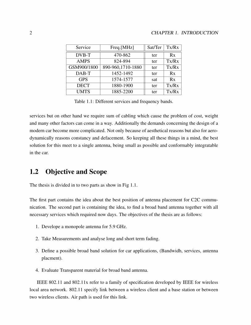
Suppose we are moving on highway, an accident that happened just a minute ago after certaindistance to our moving place. We don’t have any chance but to rush towards the end of theresulting traffic jam and we can imagine our reaction when the end of the jamming is suddenlyappears. We don’t have any chance to know about what’s going on with traffic after a fewdistances to us. Extreme traffic congestion sets in when vehicles are fully stopped for periods oftime at the accident place and this will cause a huge traffic jam. Due to the accident the freeway issporadic and there is an extensive line up of vehicles that are waiting the situation to regularize.If we get some electronic assist which already update us about the imminent situation and onbehalf of this electronic assist we can slow down the car, long before the danger comes intosight. And we can be free from extensive line up of vehicles.On a frosty morning, imagine if the car 30 meter ahead of you could somehow alert you to blackice on an off-ramp. You can slow down, and your car’s electronic stability system could even takepreliminary steps to anticipate the situation. Witness C2C communication, the next step in safetytechnology. Its something experts in organizations from the Center for Automotive Researchto economic consultancy Global Insight have mulled for years now, and theres even a federalprogram, called Intelligent Transportation Systems, to coordinate such efforts.[03]. Number ofradio services are link with vehicles now days. Due to upcoming technology, the number ofradio services for mobile application will increase. All these services should also be availablesin vehicles. The different services are using several frequency bands as shown in Table 1.1.
One solution for to cover several frequency bands is, number of antennas. Atleast five an-tennas are required in a car, for key services. Number of antennas can facilitate us with many
1
2 CHAPTER 1. INTRODUCTION
Service Freq.[MHz] Sat/Ter Tx/Rx
DVB-T 470-862 ter RxAMPS 824-894 ter Tx/Rx
GSM900/1800 890-960,1710-1880 ter Tx/RxDAB-T 1452-1492 ter Rx
GPS 1574-1577 sat RxDECT 1880-1900 ter Tx/RxUMTS 1885-2200 ter Tx/Rx
Table 1.1: Different services and frequency bands.
services but on other hand we require sum of cabling which cause the problem of cost, weightand many other factors can come in a way. Additionally the demands concerning the design of amodern car become more complicated. Not only because of aesthetical reasons but also for aero-dynamically reasons constancy and defacement. So keeping all these things in a mind, the bestsolution for this meet to a single antenna, being small as possible and conformably integratablein the car.
1.2 Objective and Scope
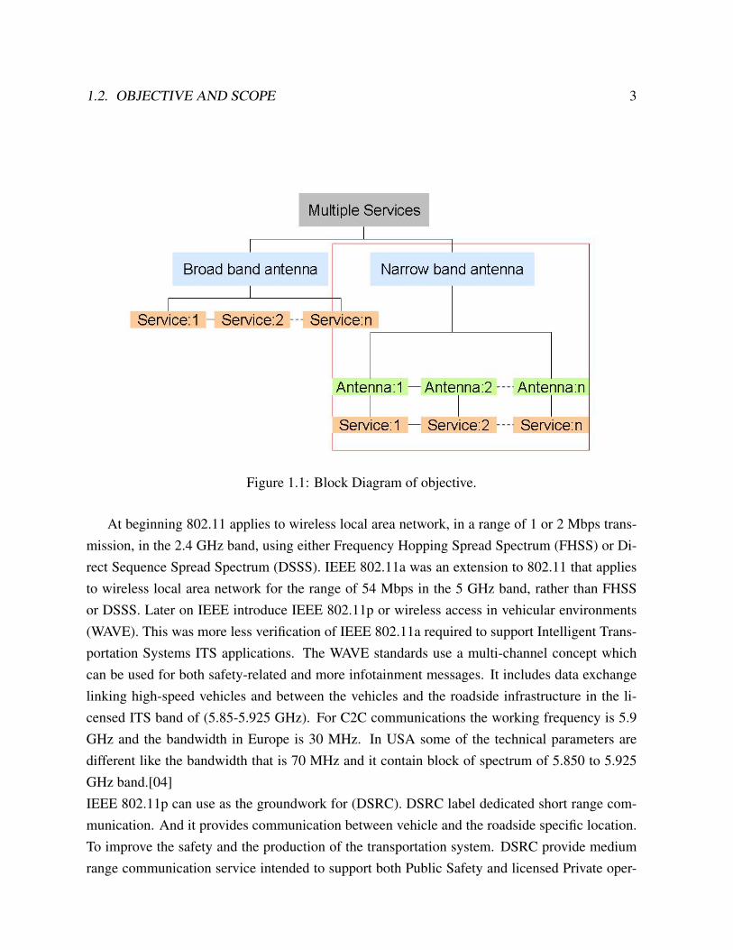
The thesis is divided in to two parts as show in Fig 1.1.
The first part contains the idea about the best position of antenna placement for C2C commu-nication. The second part is containing the idea, to find a broad band antenna together with allnecessary services which required now days. The objectives of the thesis are as follows:
1. Develope a monopole antenna for 5.9 GHz.
2. Take Measurements and analyse long and short term fading.
3. Define a possible broad band solution for car applications, (Bandwidh, services, antennaplacment).
4. Evaluate Transparent material for broad band antenna.
IEEE 802.11 and 802.11x refer to a family of specification developed by IEEE for wirelesslocal area network. 802.11 specify link between a wireless client and a base station or betweentwo wireless clients. Air path is used for this link.
1.2. OBJECTIVE AND SCOPE 3
Figure 1.1: Block Diagram of objective.
At beginning 802.11 applies to wireless local area network, in a range of 1 or 2 Mbps trans-mission, in the 2.4 GHz band, using either Frequency Hopping Spread Spectrum (FHSS) or Di-rect Sequence Spread Spectrum (DSSS). IEEE 802.11a was an extension to 802.11 that appliesto wireless local area network for the range of 54 Mbps in the 5 GHz band, rather than FHSSor DSSS. Later on IEEE introduce IEEE 802.11p or wireless access in vehicular environments(WAVE). This was more less verification of IEEE 802.11a required to support Intelligent Trans-portation Systems ITS applications. The WAVE standards use a multi-channel concept whichcan be used for both safety-related and more infotainment messages. It includes data exchangelinking high-speed vehicles and between the vehicles and the roadside infrastructure in the li-censed ITS band of (5.85-5.925 GHz). For C2C communications the working frequency is 5.9GHz and the bandwidth in Europe is 30 MHz. In USA some of the technical parameters aredifferent like the bandwidth that is 70 MHz and it contain block of spectrum of 5.850 to 5.925GHz band.[04]IEEE 802.11p can use as the groundwork for (DSRC). DSRC label dedicated short range com-munication. And it provides communication between vehicle and the roadside specific location.To improve the safety and the production of the transportation system. DSRC provide mediumrange communication service intended to support both Public Safety and licensed Private oper-
4 CHAPTER 1. INTRODUCTION
ations over roadside-to-vehicle and vehicle-to-vehicle communication channels. DSRC containoperational frequencies and system bandwidth, but also allow for operational frequencies whichare covered with in Europe by national regulation.Chpter 1 and 2 is based on basic informations. Chapter 3 is based on ray tracing simulationfor LOS and NLOS. Chapter 4 describe whole measurement setup and measurements for C2Ccommunication. Chapter 5 explain about different kind of broad band antennas and there advan-tages and disadvantages. Chapter 6 shows the best position for antenna in the car and transparentmaterial. Chapter 7contain on simulation of broad band antennas.
Chapter 2
Channel Characteristics
Channel is always characterised by different parameters, this chapter contains a description ofthe different parameters.
2.1 Narrow-band Analysis
In radio communication when the message bandwidth is less then coherence bandwidth, then itcalled Narrow-band. Narrow-band is analysed by the fading components (long term fading andshort term fading).
2.1.1 Long-Term Fading
Long term fading behave in its statistical properties quite similar to a log normal processes. Withsuch processes the slow fluctuations of local mean value of receive signal which is determine byshadowing effects can be reproduced. The channel transfer function HTP (t) can be divided intoa short-term and a long-term fading component.
∣∣HT P (t) = l(t)s(t)∣∣ (2.1)
The long-term fading component l(t) is the result of averaging |HT P (t)| during the desiredsample time Ts.
l(t) = 1/Ts
∫ t+Ts/2
t−Ts/2
|HT P |(∈)d ∈ (2.2)
As it is shown in the Fig 2.1. the long-term fading is the slow change of the signal strength
5
6 CHAPTER 2. CHANNEL CHARACTERISTICS
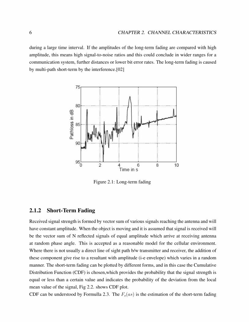
during a large time interval. If the amplitudes of the long-term fading are compared with highamplitude, this means high signal-to-noise ratios and this could conclude in wider ranges for acommunication system, further distances or lower bit error rates. The long-term fading is causedby multi-path short-term by the interference.[02]
Figure 2.1: Long-term fading
2.1.2 Short-Term Fading
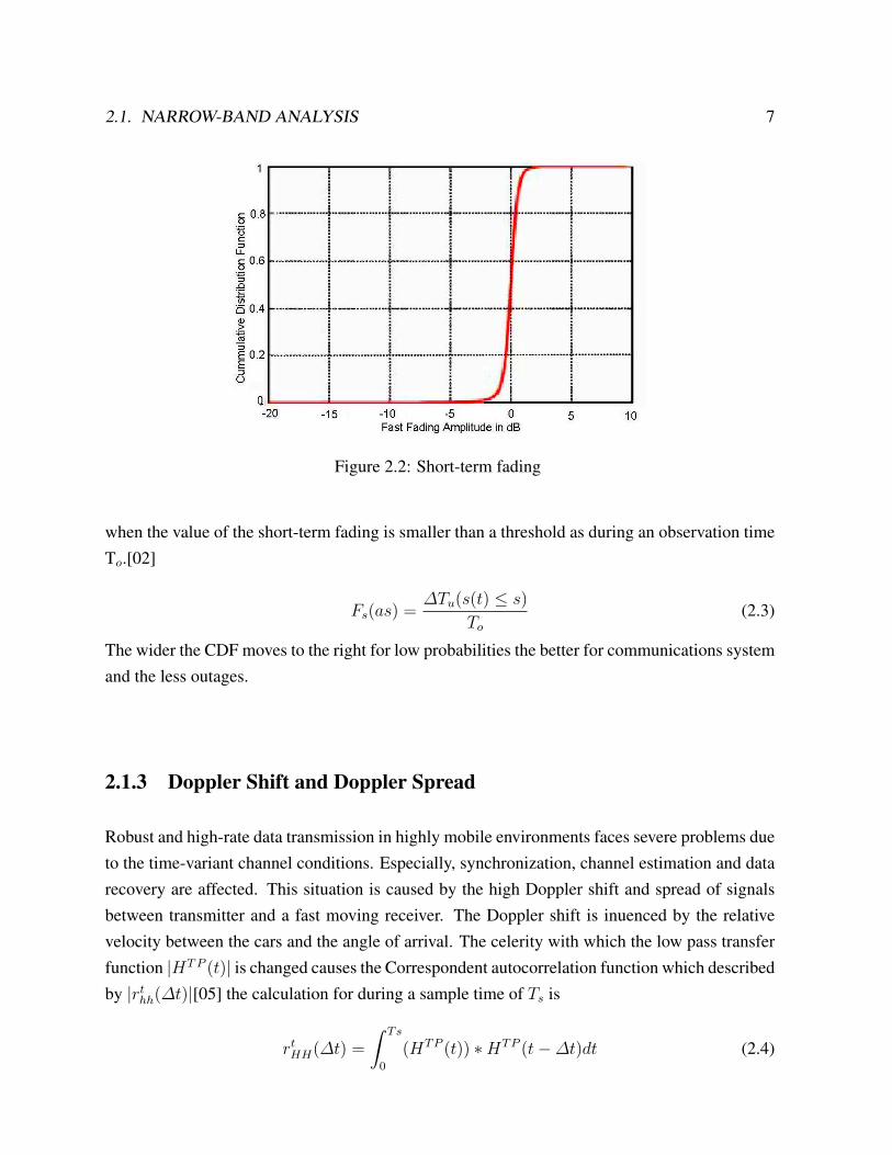
Received signal strength is formed by vector sum of various signals reaching the antenna and willhave constant amplitude. When the object is moving and it is assumed that signal is received willbe the vector sum of N reflected signals of equal amplitude which arrive at receiving antennaat random phase angle. This is accepted as a reasonable model for the cellular environment.Where there is not usually a direct line of sight path b/w transmitter and receiver, the addition ofthese component give rise to a resultant with amplitude (i-e envelope) which varies in a randommanner. The short-term fading can be plotted by different forms, and in this case the CumulativeDistribution Function (CDF) is chosen,which provides the probability that the signal strength isequal or less than a certain value and indicates the probability of the deviation from the localmean value of the signal, Fig 2.2. shows CDF plot.CDF can be understood by Formulla 2.3. The Fs(as) is the estimation of the short-term fading
2.1. NARROW-BAND ANALYSIS 7
Figure 2.2: Short-term fading
when the value of the short-term fading is smaller than a threshold as during an observation timeTo.[02]
Fs(as) =∆Tu(s(t) ≤ s)
To
(2.3)
The wider the CDF moves to the right for low probabilities the better for communications systemand the less outages.
2.1.3 Doppler Shift and Doppler Spread
Robust and high-rate data transmission in highly mobile environments faces severe problems dueto the time-variant channel conditions. Especially, synchronization, channel estimation and datarecovery are affected. This situation is caused by the high Doppler shift and spread of signalsbetween transmitter and a fast moving receiver. The Doppler shift is inuenced by the relativevelocity between the cars and the angle of arrival. The celerity with which the low pass transferfunction |HT P (t)| is changed causes the Correspondent autocorrelation function which describedby |rt
hh(∆t)|[05] the calculation for during a sample time of Ts is
rtHH(∆t) =
∫ Ts
0
(HTP (t)) ∗HTP (t−∆t)dt (2.4)
8 CHAPTER 2. CHANNEL CHARACTERISTICS
The Fourier transformation for the time variant autocorrelation function |rthh(∆t)| is the Doppler
spectrum SHH(fD):rthh(∆t) → •SHH(fD) = |HTP
D (fD)|2 (2.5)
HTPD (fD) → •HTP (t) (2.6)
The measure of the Doppler spectrum SHH(fD) in a determined moment t = t0 is
S(fD, t0) =
N(t0)∑n=1
|An(t0)|2 δ(fD − fD, n) (2.7)
The Doppler spectrum is characterized by two dierent parameters, the mean Doppler fD and theDoppler spreadbσfD
. The mean Doppler is the average value:
fD =
∑−∞∞ fDSHH(fD)dfD∫∞∞ SHH(fD)dfD.
(2.8)
The Doppler spread is deined as two times the variation of the Doppler spectrum, if the Dopplerspectrum is assumed as a probability density function.
σfD= 2
√∫ −∞∞ f 2
DSHH(fD)dfD∫∞∞ SHH(fD)dfD
− f 2D (2.9)
The higher the value of the Doppler spread σfD, the faster the changes in the channel and the
more difficult would be to receive the transmitting signal correctly. If the Doppler spread issmaller than the bandwidth of the transmitted signal, most of the transmitted power will be in theband.[02]
Chapter 3
Simulation Results
This chapter is including the analysis of simulated scenarios. Two different kinds of scenariosare evaluated; LOS (line os sight) and NLOS (no line of sight), both are urban scenarios.
3.1 LOS Scenario
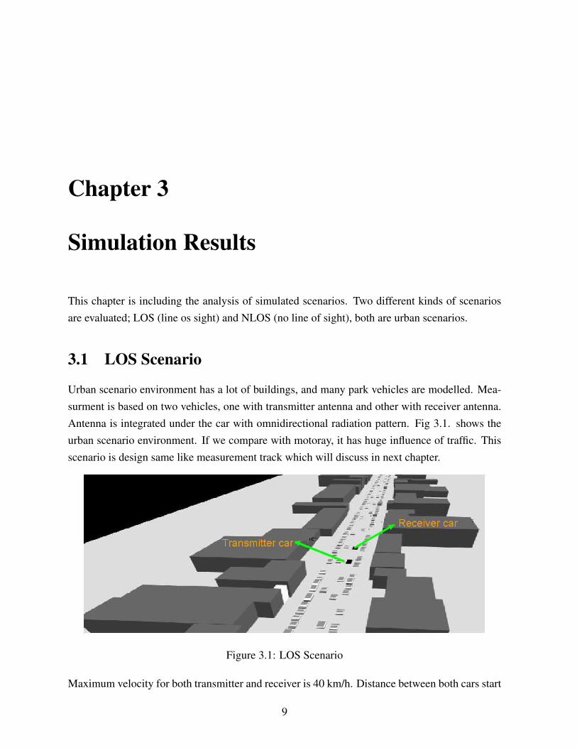
Urban scenario environment has a lot of buildings, and many park vehicles are modelled. Mea-surment is based on two vehicles, one with transmitter antenna and other with receiver antenna.Antenna is integrated under the car with omnidirectional radiation pattern. Fig 3.1. shows theurban scenario environment. If we compare with motoray, it has huge influence of traffic. Thisscenario is design same like measurement track which will discuss in next chapter.
Figure 3.1: LOS Scenario
Maximum velocity for both transmitter and receiver is 40 km/h. Distance between both cars start
9
10 CHAPTER 3. SIMULATION RESULTS
from 47.8 m and then it change with time, distance become close after each second and finallyreached at 38.2 m. Distance change with respect to traffic.
3.1.1 Long-Term Fading
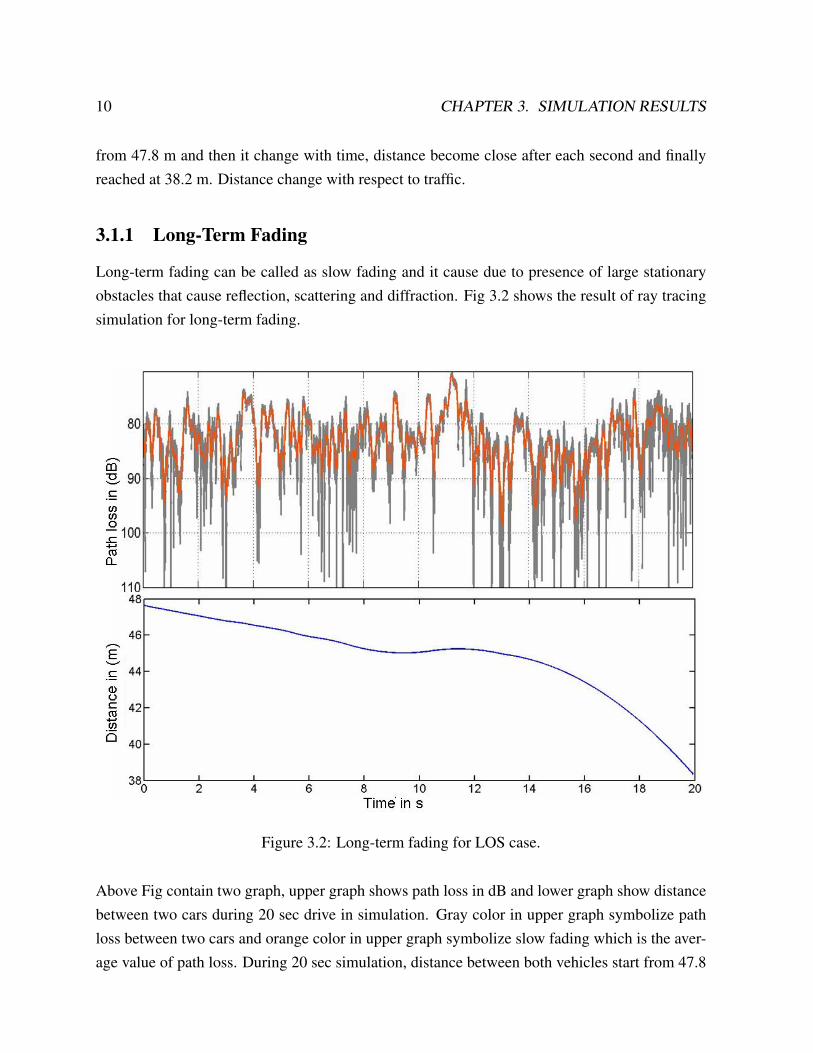
Long-term fading can be called as slow fading and it cause due to presence of large stationaryobstacles that cause reflection, scattering and diffraction. Fig 3.2 shows the result of ray tracingsimulation for long-term fading.
Figure 3.2: Long-term fading for LOS case.
Above Fig contain two graph, upper graph shows path loss in dB and lower graph show distancebetween two cars during 20 sec drive in simulation. Gray color in upper graph symbolize pathloss between two cars and orange color in upper graph symbolize slow fading which is the aver-age value of path loss. During 20 sec simulation, distance between both vehicles start from 47.8
3.1. LOS SCENARIO 11
m and then goes down till 38.2 m. A lot of buildings, and a lot of parked vehicles are modelledin this scenario. A receiver antenna received sum of reflecting signal from different surroundingobject. At 12 sec, distance between two cars is near to 46 m, and the signal is constructive atthis stage. At very next sec distance between two cars is reduced but path loss increase due todestructive interference. Average path loss retain between 80 dB to 90 dB, resultanat path losscan work for real environment.
3.1.2 Short-Term Fading
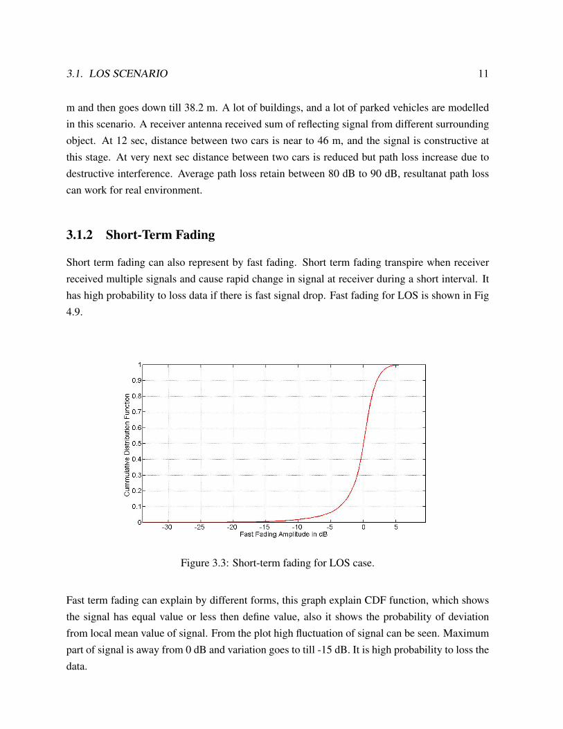
Short term fading can also represent by fast fading. Short term fading transpire when receiverreceived multiple signals and cause rapid change in signal at receiver during a short interval. Ithas high probability to loss data if there is fast signal drop. Fast fading for LOS is shown in Fig4.9.
Figure 3.3: Short-term fading for LOS case.
Fast term fading can explain by different forms, this graph explain CDF function, which showsthe signal has equal value or less then define value, also it shows the probability of deviationfrom local mean value of signal. From the plot high fluctuation of signal can be seen. Maximumpart of signal is away from 0 dB and variation goes to till -15 dB. It is high probability to loss thedata.
12 CHAPTER 3. SIMULATION RESULTS
3.2 NLOS Scenario
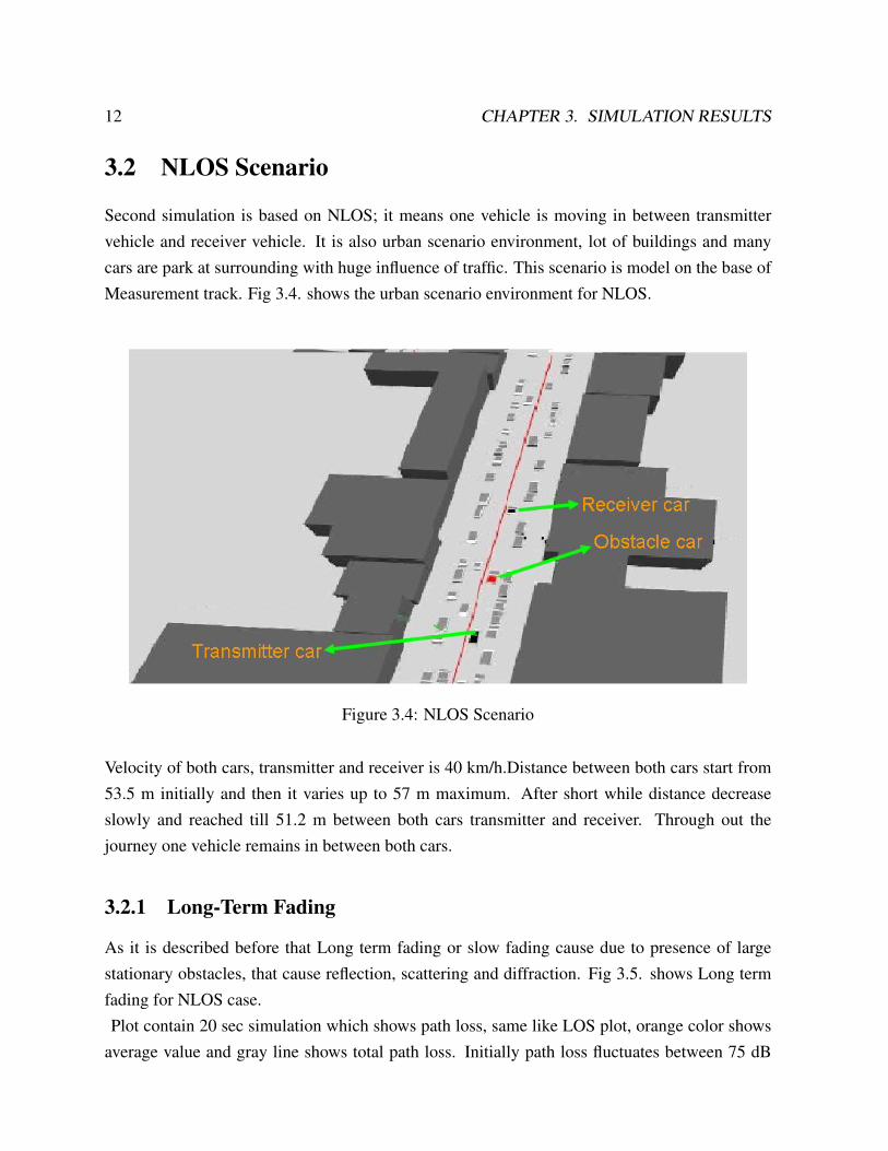
Second simulation is based on NLOS; it means one vehicle is moving in between transmittervehicle and receiver vehicle. It is also urban scenario environment, lot of buildings and manycars are park at surrounding with huge influence of traffic. This scenario is model on the base ofMeasurement track. Fig 3.4. shows the urban scenario environment for NLOS.
Figure 3.4: NLOS Scenario
Velocity of both cars, transmitter and receiver is 40 km/h.Distance between both cars start from53.5 m initially and then it varies up to 57 m maximum. After short while distance decreaseslowly and reached till 51.2 m between both cars transmitter and receiver. Through out thejourney one vehicle remains in between both cars.
3.2.1 Long-Term Fading
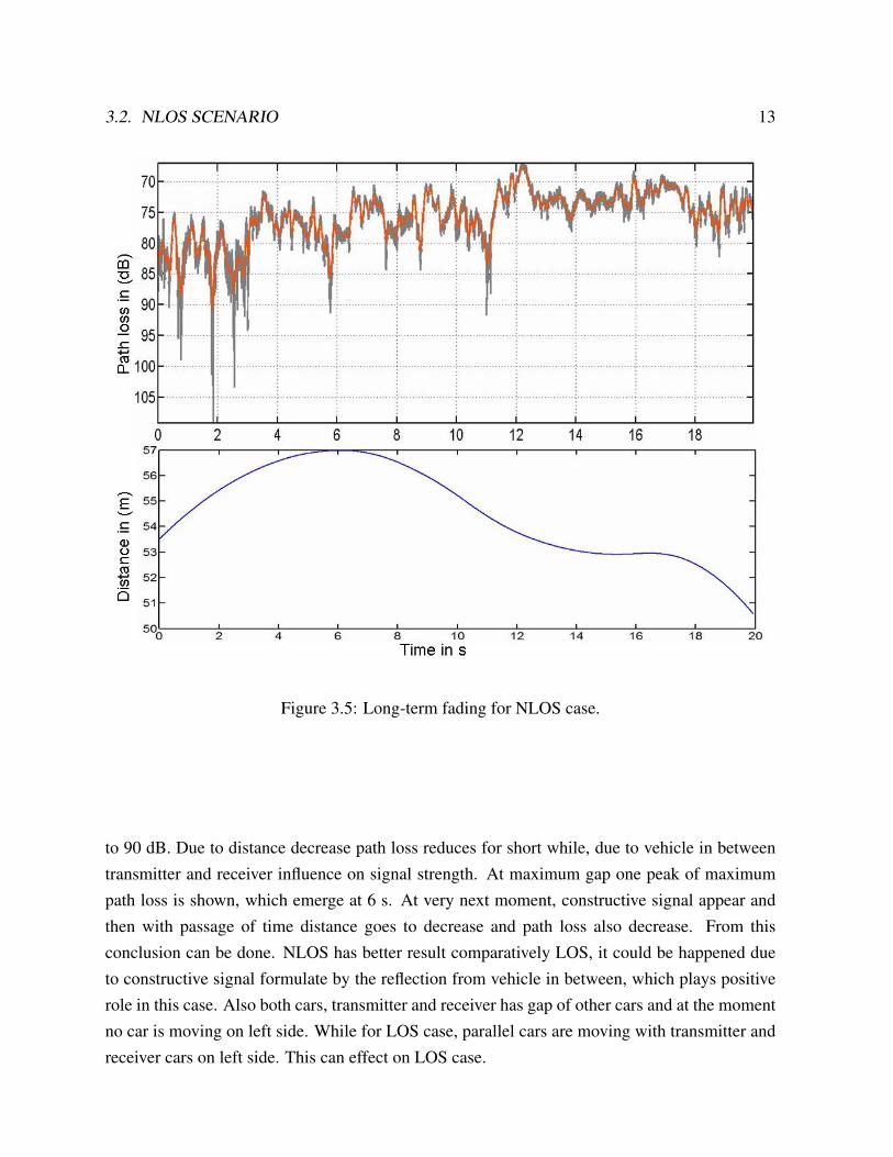
As it is described before that Long term fading or slow fading cause due to presence of largestationary obstacles, that cause reflection, scattering and diffraction. Fig 3.5. shows Long termfading for NLOS case.Plot contain 20 sec simulation which shows path loss, same like LOS plot, orange color shows
average value and gray line shows total path loss. Initially path loss fluctuates between 75 dB
3.2. NLOS SCENARIO 13
Figure 3.5: Long-term fading for NLOS case.
to 90 dB. Due to distance decrease path loss reduces for short while, due to vehicle in betweentransmitter and receiver influence on signal strength. At maximum gap one peak of maximumpath loss is shown, which emerge at 6 s. At very next moment, constructive signal appear andthen with passage of time distance goes to decrease and path loss also decrease. From thisconclusion can be done. NLOS has better result comparatively LOS, it could be happened dueto constructive signal formulate by the reflection from vehicle in between, which plays positiverole in this case. Also both cars, transmitter and receiver has gap of other cars and at the momentno car is moving on left side. While for LOS case, parallel cars are moving with transmitter andreceiver cars on left side. This can effect on LOS case.
14 CHAPTER 3. SIMULATION RESULTS
3.2.2 Short-Term Fading
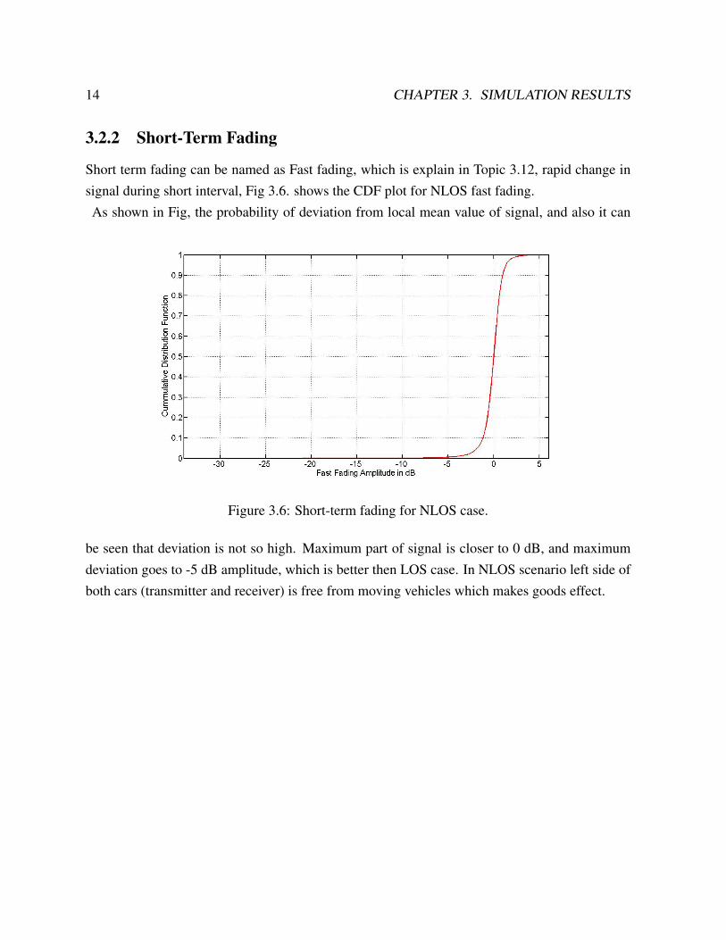
Short term fading can be named as Fast fading, which is explain in Topic 3.12, rapid change insignal during short interval, Fig 3.6. shows the CDF plot for NLOS fast fading.As shown in Fig, the probability of deviation from local mean value of signal, and also it can
Figure 3.6: Short-term fading for NLOS case.
be seen that deviation is not so high. Maximum part of signal is closer to 0 dB, and maximumdeviation goes to -5 dB amplitude, which is better then LOS case. In NLOS scenario left side ofboth cars (transmitter and receiver) is free from moving vehicles which makes goods effect.
Chapter 4
Measurements and Ray tracing results
4.1 Best Position for Antenna
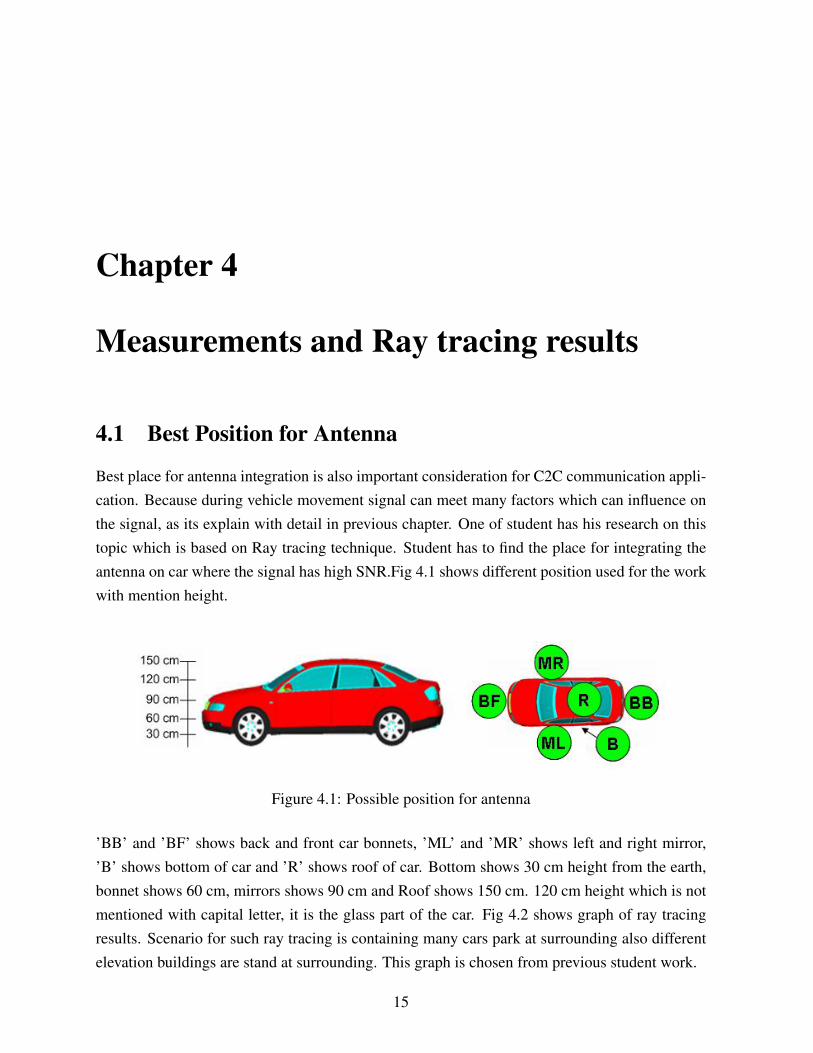
Best place for antenna integration is also important consideration for C2C communication appli-cation. Because during vehicle movement signal can meet many factors which can influence onthe signal, as its explain with detail in previous chapter. One of student has his research on thistopic which is based on Ray tracing technique. Student has to find the place for integrating theantenna on car where the signal has high SNR.Fig 4.1 shows different position used for the workwith mention height.
Figure 4.1: Possible position for antenna
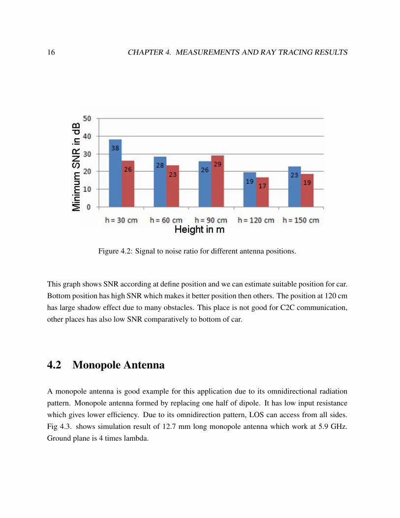
’BB’ and ’BF’ shows back and front car bonnets, ’ML’ and ’MR’ shows left and right mirror,’B’ shows bottom of car and ’R’ shows roof of car. Bottom shows 30 cm height from the earth,bonnet shows 60 cm, mirrors shows 90 cm and Roof shows 150 cm. 120 cm height which is notmentioned with capital letter, it is the glass part of the car. Fig 4.2 shows graph of ray tracingresults. Scenario for such ray tracing is containing many cars park at surrounding also differentelevation buildings are stand at surrounding. This graph is chosen from previous student work.
15
16 CHAPTER 4. MEASUREMENTS AND RAY TRACING RESULTS
Figure 4.2: Signal to noise ratio for different antenna positions.
This graph shows SNR according at define position and we can estimate suitable position for car.Bottom position has high SNR which makes it better position then others. The position at 120 cmhas large shadow effect due to many obstacles. This place is not good for C2C communication,other places has also low SNR comparatively to bottom of car.
4.2 Monopole Antenna
A monopole antenna is good example for this application due to its omnidirectional radiationpattern. Monopole antenna formed by replacing one half of dipole. It has low input resistancewhich gives lower efficiency. Due to its omnidirection pattern, LOS can access from all sides.Fig 4.3. shows simulation result of 12.7 mm long monopole antenna which work at 5.9 GHz.Ground plane is 4 times lambda.
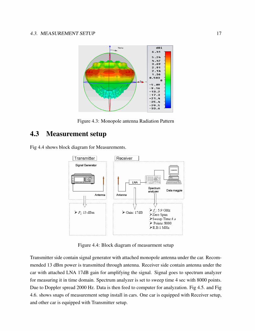
4.3. MEASUREMENT SETUP 17
Figure 4.3: Monopole antenna Radiation Pattern
4.3 Measurement setup
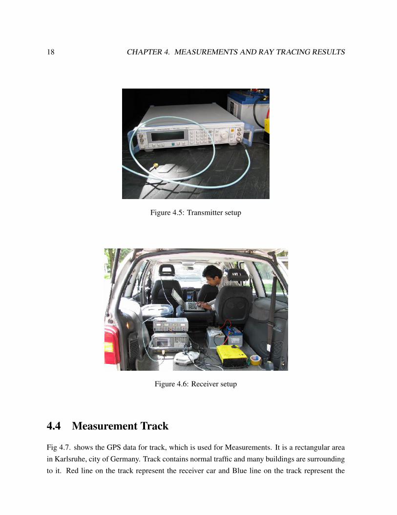
Fig 4.4 shows block diagram for Measurements.
Figure 4.4: Block diagram of measurment setup
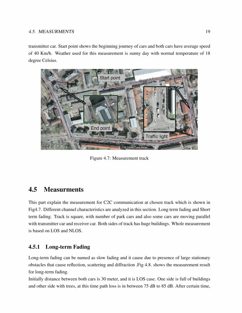
Transmitter side contain signal generator with attached monopole antenna under the car. Recom-mended 13 dBm power is transmitted through antenna. Receiver side contain antenna under thecar with attached LNA 17dB gain for amplifying the signal. Signal goes to spectrum analyzerfor measuring it in time domain. Spectrum analyzer is set to sweep time 4 sec with 8000 points.Due to Doppler spread 2000 Hz. Data is then feed to computer for analyzation. Fig 4.5. and Fig4.6. shows snaps of measurement setup install in cars. One car is equipped with Receiver setup,and other car is equipped with Transmitter setup.
18 CHAPTER 4. MEASUREMENTS AND RAY TRACING RESULTS
Figure 4.5: Transmitter setup
Figure 4.6: Receiver setup
4.4 Measurement Track
Fig 4.7. shows the GPS data for track, which is used for Measurements. It is a rectangular areain Karlsruhe, city of Germany. Track contains normal traffic and many buildings are surroundingto it. Red line on the track represent the receiver car and Blue line on the track represent the
4.5. MEASURMENTS 19
transmitter car. Start point shows the beginning journey of cars and both cars have average speedof 40 Km/h. Weather used for this measurement is sunny day with normal temperature of 18degree Celsius.
Figure 4.7: Measurement track
4.5 Measurments
This part explain the measurement for C2C communication at chosen track which is shown inFig4.7. Different channel characteristics are analyzed in this section. Long term fading and Shortterm fading. Track is square, with number of park cars and also some cars are moving parallelwith transmitter car and receiver car. Both sides of track has huge buildings. Whole measurementis based on LOS and NLOS.
4.5.1 Long-term Fading
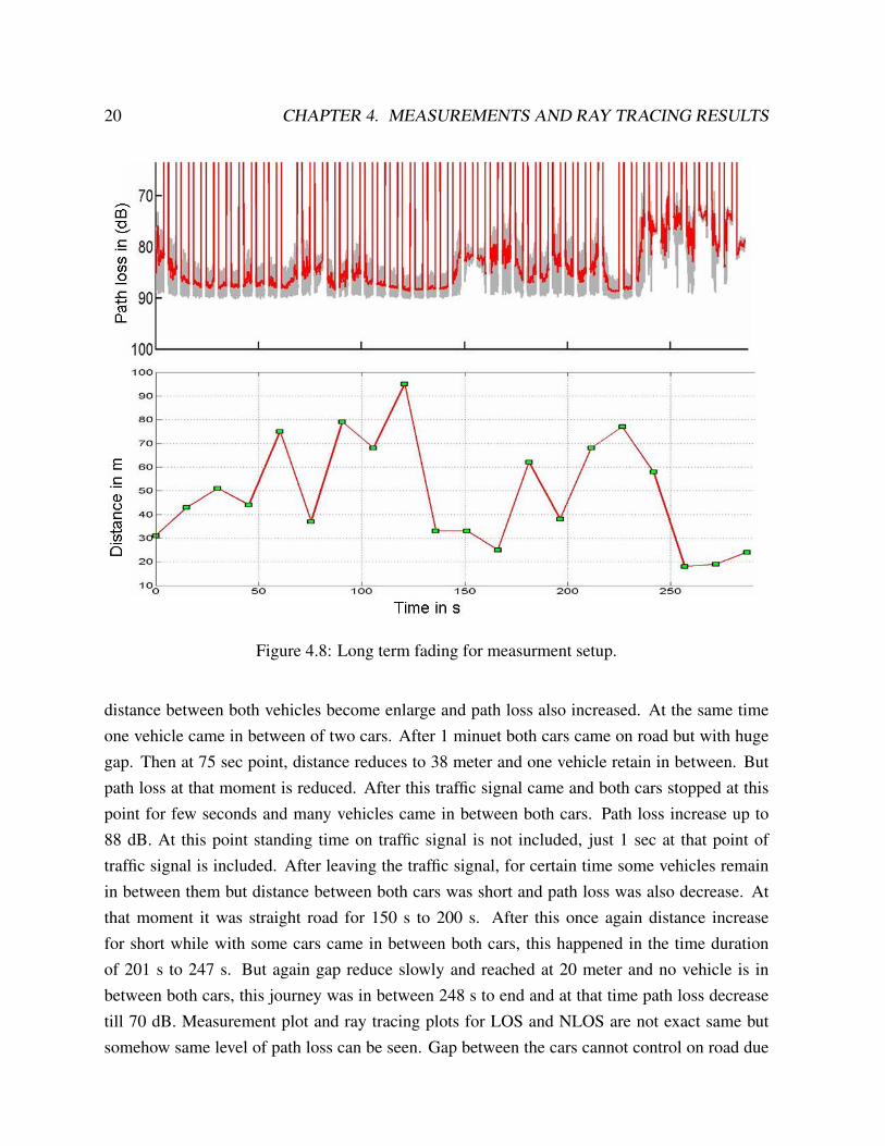
Long-term fading can be named as slow fading and it cause due to presence of large stationaryobstacles that cause reflection, scattering and diffraction .Fig 4.8. shows the measurement resultfor long-term fading.Initially distance between both cars is 30 meter, and it is LOS case. One side is full of buildingsand other side with trees, at this time path loss is in between 75 dB to 85 dB. After certain time,
20 CHAPTER 4. MEASUREMENTS AND RAY TRACING RESULTS
Figure 4.8: Long term fading for measurment setup.
distance between both vehicles become enlarge and path loss also increased. At the same timeone vehicle came in between of two cars. After 1 minuet both cars came on road but with hugegap. Then at 75 sec point, distance reduces to 38 meter and one vehicle retain in between. Butpath loss at that moment is reduced. After this traffic signal came and both cars stopped at thispoint for few seconds and many vehicles came in between both cars. Path loss increase up to88 dB. At this point standing time on traffic signal is not included, just 1 sec at that point oftraffic signal is included. After leaving the traffic signal, for certain time some vehicles remainin between them but distance between both cars was short and path loss was also decrease. Atthat moment it was straight road for 150 s to 200 s. After this once again distance increasefor short while with some cars came in between both cars, this happened in the time durationof 201 s to 247 s. But again gap reduce slowly and reached at 20 meter and no vehicle is inbetween both cars, this journey was in between 248 s to end and at that time path loss decreasetill 70 dB. Measurement plot and ray tracing plots for LOS and NLOS are not exact same butsomehow same level of path loss can be seen. Gap between the cars cannot control on road due
4.5. MEASURMENTS 21
to traffic, and road has friction which is not included in ray tracing simulation also antenna hasbend radiation patterns, it is not exact on the corners so we don’t have perfect LOS for radiationpattern as it is shown in Fig 4.3. Actually antenna under the car can meet some pipes which canobstruct the signal. But still it works for C2C communication application.
4.5.2 Short-term Fading
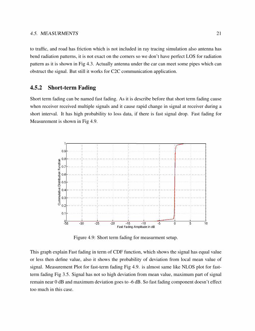
Short term fading can be named fast fading. As it is describe before that short term fading causewhen receiver received multiple signals and it cause rapid change in signal at receiver during ashort interval. It has high probability to loss data, if there is fast signal drop. Fast fading forMeasurement is shown in Fig 4.9.
Figure 4.9: Short term fading for measurment setup.
This graph explain Fast fading in term of CDF function, which shows the signal has equal valueor less then define value, also it shows the probability of deviation from local mean value ofsignal. Measurement Plot for fast-term fading Fig 4.9. is almost same like NLOS plot for fast-term fading Fig 3.5. Signal has not so high deviation from mean value, maximum part of signalremain near 0 dB and maximum deviation goes to -6 dB. So fast fading component doesn’t effecttoo much in this case.

22 CHAPTER 4. MEASUREMENTS AND RAY TRACING RESULTS
Chapter 5
Broad Band Antenna basics
This chapter will discuss in detail about the broad band antenna. In Telecommunication fieldBroad band technology is a concept in which number of frequencies can be include in a singlemethod. Wider bandwidth has capacity to carry more information. A Single Broadband antennais able to cover many narrow band services, which is an option for reduction of space needed forthe radiators.
5.1 Gain
Gain is important consideration before choosing the antenna. The gain is a measure of howmuch of the input power is intense in a particular direction. It is expressed with respect toa hypothetical isotropic antenna, which radiates equally in all directions. Radiation intensityfrom a lossless isotropic antenna equals the power into the antenna divided by a solid angle of4πsteradians.
5.2 Radiation pattern
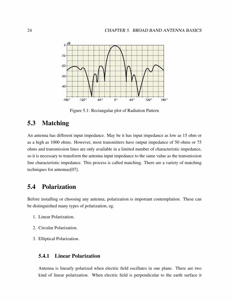
The radiation pattern or antenna pattern describes the relative strength of the radiated field invarious directions from the antenna, at a constant distance. The radiation pattern is a receptionpattern as well, since it also describes the receiving properties of the antenna. The followingfigure 5.1. shows a rectangular plot presentation for radiation pattern.[06]
23
24 CHAPTER 5. BROAD BAND ANTENNA BASICS
Figure 5.1: Rectangular plot of Radiation Pattern
5.3 Matching
An antenna has different input impedance. May be it has input impedance as low as 15 ohm oras a high as 1000 ohms. However, most transmitters have output impedance of 50 ohms or 75ohms and transmission lines are only available in a limited number of characteristic impedance,so it is necessary to transform the antenna input impedance to the same value as the transmissionline characteristic impedance. This process is called matching. There are a variety of matchingtechniques for antennas[07].
5.4 Polarization
Before installing or choosing any antenna, polarization is important contemplation. These canbe distinguished many types of polarization, eg.
1. Linear Polarization.
2. Circular Polarization.
3. Elliptical Polarization.
5.4.1 Linear Polarization
Antenna is linearly polarized when electric field oscillates in one plane. There are twokind of linear polarization. When electric field is perpendicular to the earth surface it
5.4. POLARIZATION 25
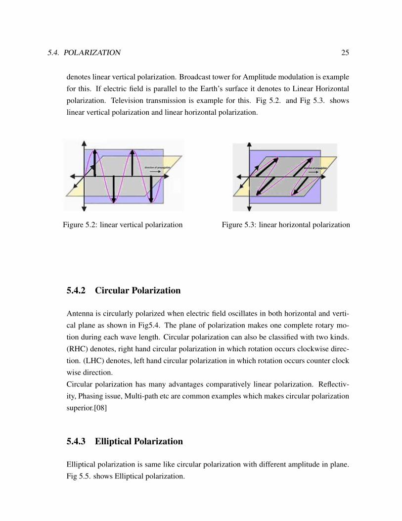
denotes linear vertical polarization. Broadcast tower for Amplitude modulation is examplefor this. If electric field is parallel to the Earth’s surface it denotes to Linear Horizontalpolarization. Television transmission is example for this. Fig 5.2. and Fig 5.3. showslinear vertical polarization and linear horizontal polarization.
Figure 5.2: linear vertical polarization Figure 5.3: linear horizontal polarization
5.4.2 Circular Polarization
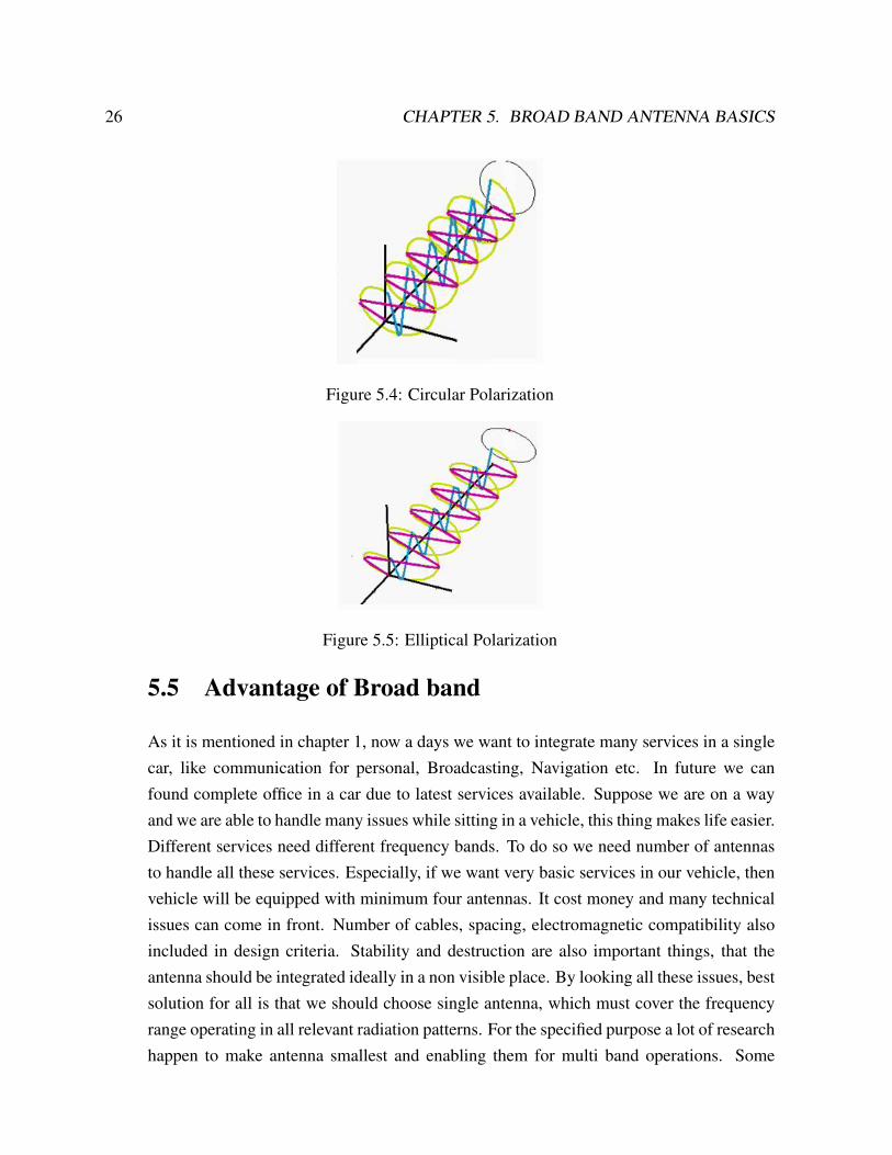
Antenna is circularly polarized when electric field oscillates in both horizontal and verti-cal plane as shown in Fig5.4. The plane of polarization makes one complete rotary mo-tion during each wave length. Circular polarization can also be classified with two kinds.(RHC) denotes, right hand circular polarization in which rotation occurs clockwise direc-tion. (LHC) denotes, left hand circular polarization in which rotation occurs counter clockwise direction.Circular polarization has many advantages comparatively linear polarization. Reflectiv-ity, Phasing issue, Multi-path etc are common examples which makes circular polarizationsuperior.[08]
5.4.3 Elliptical Polarization
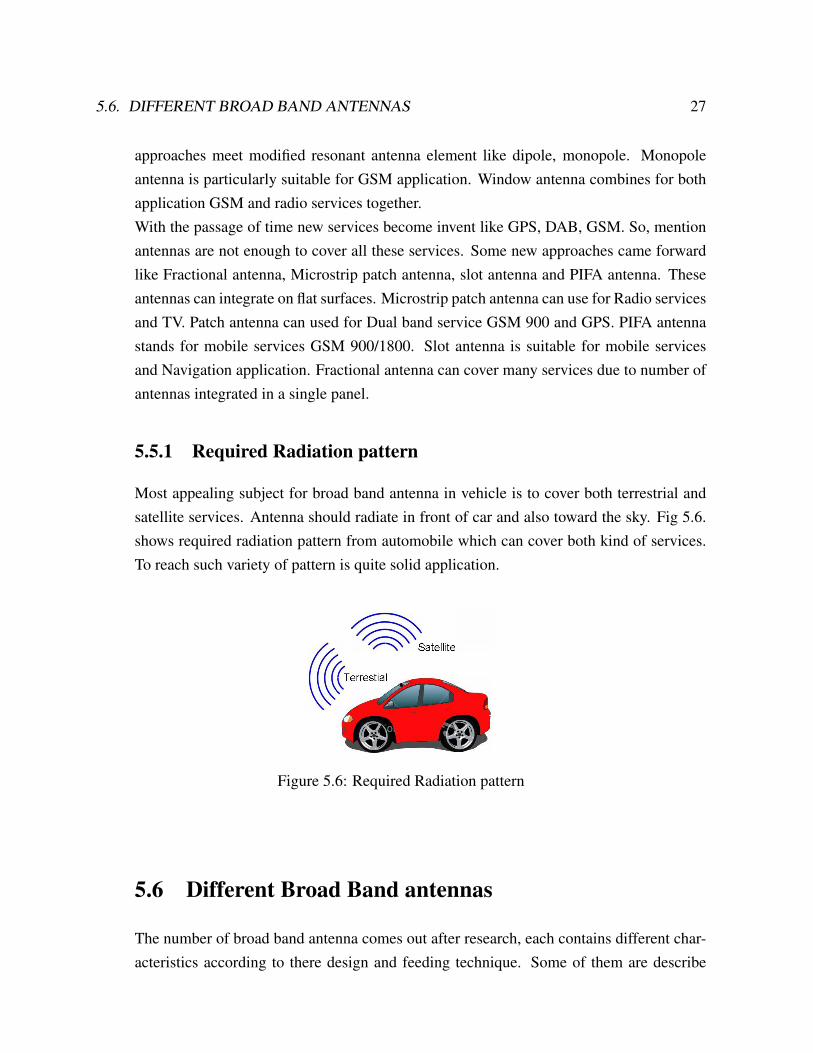
Elliptical polarization is same like circular polarization with different amplitude in plane.Fig 5.5. shows Elliptical polarization.
26 CHAPTER 5. BROAD BAND ANTENNA BASICS
Figure 5.4: Circular Polarization
Figure 5.5: Elliptical Polarization
5.5 Advantage of Broad band
As it is mentioned in chapter 1, now a days we want to integrate many services in a singlecar, like communication for personal, Broadcasting, Navigation etc. In future we canfound complete office in a car due to latest services available. Suppose we are on a wayand we are able to handle many issues while sitting in a vehicle, this thing makes life easier.Different services need different frequency bands. To do so we need number of antennasto handle all these services. Especially, if we want very basic services in our vehicle, thenvehicle will be equipped with minimum four antennas. It cost money and many technicalissues can come in front. Number of cables, spacing, electromagnetic compatibility alsoincluded in design criteria. Stability and destruction are also important things, that theantenna should be integrated ideally in a non visible place. By looking all these issues, bestsolution for all is that we should choose single antenna, which must cover the frequencyrange operating in all relevant radiation patterns. For the specified purpose a lot of researchhappen to make antenna smallest and enabling them for multi band operations. Some
5.6. DIFFERENT BROAD BAND ANTENNAS 27
approaches meet modified resonant antenna element like dipole, monopole. Monopoleantenna is particularly suitable for GSM application. Window antenna combines for bothapplication GSM and radio services together.With the passage of time new services become invent like GPS, DAB, GSM. So, mentionantennas are not enough to cover all these services. Some new approaches came forwardlike Fractional antenna, Microstrip patch antenna, slot antenna and PIFA antenna. Theseantennas can integrate on flat surfaces. Microstrip patch antenna can use for Radio servicesand TV. Patch antenna can used for Dual band service GSM 900 and GPS. PIFA antennastands for mobile services GSM 900/1800. Slot antenna is suitable for mobile servicesand Navigation application. Fractional antenna can cover many services due to number ofantennas integrated in a single panel.
5.5.1 Required Radiation pattern
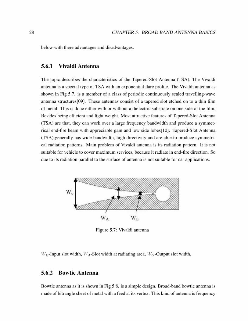
Most appealing subject for broad band antenna in vehicle is to cover both terrestrial andsatellite services. Antenna should radiate in front of car and also toward the sky. Fig 5.6.shows required radiation pattern from automobile which can cover both kind of services.To reach such variety of pattern is quite solid application.
Figure 5.6: Required Radiation pattern
5.6 Different Broad Band antennas
The number of broad band antenna comes out after research, each contains different char-acteristics according to there design and feeding technique. Some of them are describe
28 CHAPTER 5. BROAD BAND ANTENNA BASICS
below with there advantages and disadvantages.
5.6.1 Vivaldi Antenna
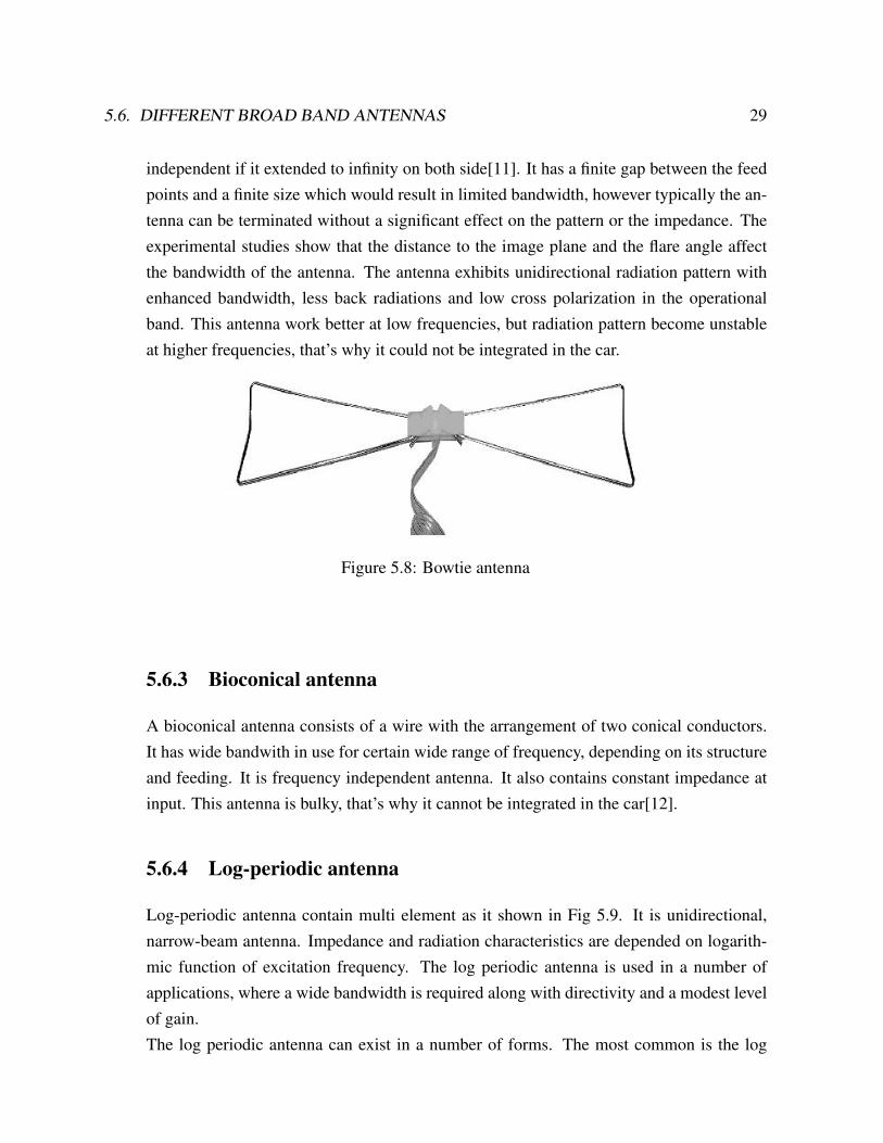
The topic describes the characteristics of the Tapered-Slot Antenna (TSA). The Vivaldiantenna is a special type of TSA with an exponential flare profile. The Vivaldi antenna asshown in Fig 5.7. is a member of a class of periodic continuously scaled travelling-waveantenna structures[09]. These antennas consist of a tapered slot etched on to a thin filmof metal. This is done either with or without a dielectric substrate on one side of the film.Besides being efficient and light weight. Most attractive features of Tapered-Slot Antenna(TSA) are that, they can work over a large frequency bandwidth and produce a symmet-rical end-fire beam with appreciable gain and low side lobes[10]. Tapered-Slot Antenna(TSA) generally has wide bandwidth, high directivity and are able to produce symmetri-cal radiation patterns. Main problem of Vivaldi antenna is its radiation pattern. It is notsuitable for vehicle to cover maximum services, because it radiate in end-fire direction. Sodue to its radiation parallel to the surface of antenna is not suitable for car applications.
Figure 5.7: Vivaldi antenna
WE-Input slot width, WA-Slot width at radiating area, WO-Output slot width,
5.6.2 Bowtie Antenna
Bowtie antenna as it is shown in Fig 5.8. is a simple design. Broad-band bowtie antenna ismade of bitrangle sheet of metal with a feed at its vertex. This kind of antenna is frequency
5.6. DIFFERENT BROAD BAND ANTENNAS 29
independent if it extended to infinity on both side[11]. It has a finite gap between the feedpoints and a finite size which would result in limited bandwidth, however typically the an-tenna can be terminated without a significant effect on the pattern or the impedance. Theexperimental studies show that the distance to the image plane and the flare angle affectthe bandwidth of the antenna. The antenna exhibits unidirectional radiation pattern withenhanced bandwidth, less back radiations and low cross polarization in the operationalband. This antenna work better at low frequencies, but radiation pattern become unstableat higher frequencies, that’s why it could not be integrated in the car.
Figure 5.8: Bowtie antenna
5.6.3 Bioconical antenna
A bioconical antenna consists of a wire with the arrangement of two conical conductors.It has wide bandwith in use for certain wide range of frequency, depending on its structureand feeding. It is frequency independent antenna. It also contains constant impedance atinput. This antenna is bulky, that’s why it cannot be integrated in the car[12].
5.6.4 Log-periodic antenna
Log-periodic antenna contain multi element as it shown in Fig 5.9. It is unidirectional,narrow-beam antenna. Impedance and radiation characteristics are depended on logarith-mic function of excitation frequency. The log periodic antenna is used in a number ofapplications, where a wide bandwidth is required along with directivity and a modest levelof gain.The log periodic antenna can exist in a number of forms. The most common is the log
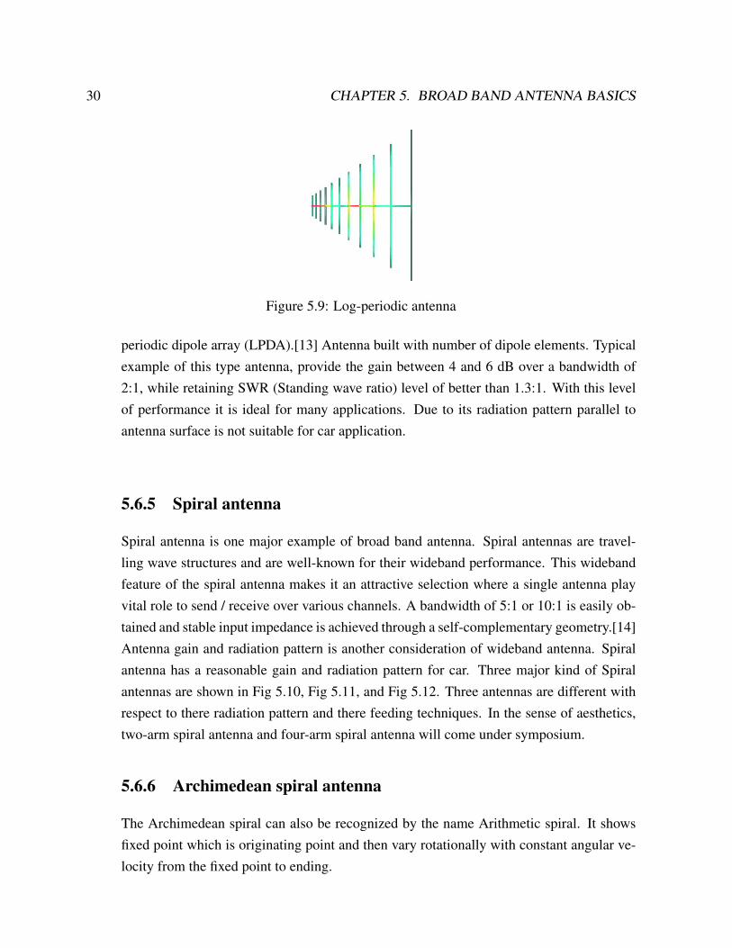
30 CHAPTER 5. BROAD BAND ANTENNA BASICS
Figure 5.9: Log-periodic antenna
periodic dipole array (LPDA).[13] Antenna built with number of dipole elements. Typicalexample of this type antenna, provide the gain between 4 and 6 dB over a bandwidth of2:1, while retaining SWR (Standing wave ratio) level of better than 1.3:1. With this levelof performance it is ideal for many applications. Due to its radiation pattern parallel toantenna surface is not suitable for car application.
5.6.5 Spiral antenna
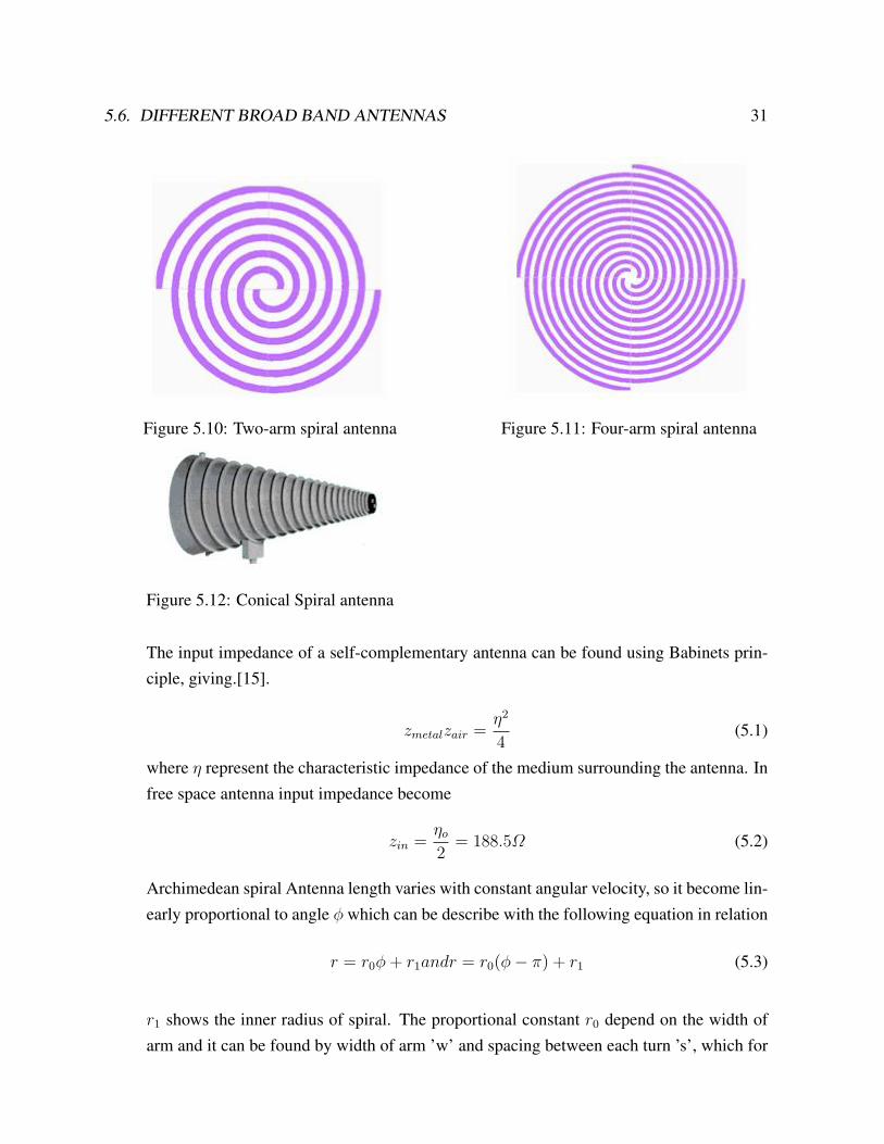
Spiral antenna is one major example of broad band antenna. Spiral antennas are travel-ling wave structures and are well-known for their wideband performance. This widebandfeature of the spiral antenna makes it an attractive selection where a single antenna playvital role to send / receive over various channels. A bandwidth of 5:1 or 10:1 is easily ob-tained and stable input impedance is achieved through a self-complementary geometry.[14]Antenna gain and radiation pattern is another consideration of wideband antenna. Spiralantenna has a reasonable gain and radiation pattern for car. Three major kind of Spiralantennas are shown in Fig 5.10, Fig 5.11, and Fig 5.12. Three antennas are different withrespect to there radiation pattern and there feeding techniques. In the sense of aesthetics,two-arm spiral antenna and four-arm spiral antenna will come under symposium.
5.6.6 Archimedean spiral antenna
The Archimedean spiral can also be recognized by the name Arithmetic spiral. It showsfixed point which is originating point and then vary rotationally with constant angular ve-locity from the fixed point to ending.
5.6. DIFFERENT BROAD BAND ANTENNAS 31
Figure 5.10: Two-arm spiral antenna Figure 5.11: Four-arm spiral antenna
Figure 5.12: Conical Spiral antenna
The input impedance of a self-complementary antenna can be found using Babinets prin-ciple, giving.[15].
zmetalzair =η2
4(5.1)
where η represent the characteristic impedance of the medium surrounding the antenna. Infree space antenna input impedance become
zin =ηo
2= 188.5Ω (5.2)
Archimedean spiral Antenna length varies with constant angular velocity, so it become lin-early proportional to angle φ which can be describe with the following equation in relation
r = r0φ+ r1andr = r0(φ− π) + r1 (5.3)
r1 shows the inner radius of spiral. The proportional constant r0 depend on the width ofarm and it can be found by width of arm ’w’ and spacing between each turn ’s’, which for
32 CHAPTER 5. BROAD BAND ANTENNA BASICS
a self complementary spiral is given by
r0 =s+ w
π=
2w
π(5.4)
the strip width can be evaluated by following equation
s =r2 − r1
2N− w = w (5.5)
By considering antenna as a self complimentary space and width can be found as
s = w =r2 − r1
4(5.6)
where r2 is the outer radius of the spiral and N is the number of turns. The above equationdescribe for two-arm Archimedean spiral. Width of four-arm spiral, can be found withfollowing equation
w4−arm =r2 − r1
8N(5.7)
and the proportionality constant
r0,4−arm =4w
π(5.8)
when the circumference of the spiral equals one wavelength then spiral start to radiate inthat region, each arm of spiral is feed 180 degree out of phase, so when the circumferenceof the spiral is one wavelength and current at complementary or opposite points on eacharm of spiral add in phase in the far field. The low frequency operating point of the spiralis determined theoretically by the outer radius and is given by
flow =c
2πr2(5.9)
where c is the speed of light. Similarly the high frequency operating point is based on theinner radius giving
fhigh =co
2πr2(5.10)
In practical the lower frequency will be greater than predicted by equation (5.9), due toreflection at the end of the spiral. The reflections can be minimized by using resistive

5.6. DIFFERENT BROAD BAND ANTENNAS 33
loading at the end of each arm or by adding conductivity loss to some part of the outer turnof each arm. Also, the high frequency limit may be less than found from (5.10) due to feedregion effects [15].

34 CHAPTER 5. BROAD BAND ANTENNA BASICS
Chapter 6
Integration of broadband spiral antennain to the car
6.1 Coplanar waveguide feeding
The CPW mode is usually the desired mode in circuits based on coplanar lines, as it is aquasi-TEM mode.[16]. Coplanar wave guide is a simple conductor line which is separatedfrom a pair of ground plane. Three lines are placed on a top of dielectric medium. Fig 6.3.shows coplanar wave guide with three lines. The line in the centre is used for conductor,and other two parallel lines are used for the grounds. In the diagram ’s’ shows the gapbetween conductor and ground lines, ’w’ shows width of conductor and ’L’ shows thelength of conductor and ground lines. These parameters play important role for matchingat input impedance. So these variables can be change according to input impedance.The Spiral antenna can be used for automotive applications. As required services in the carit is necessary that antenna should radiate in two modes. One can cover terrestrial servicesand other can cover satellite services, and this can happened by using coplanar wave guidefeed network in the centre of spiral. In the response, antenna will work in dual mode.Fou-rarm spiral is best choice for this work and coplanar transmission line is connectedorthogonally to the spiral. Conductor line of coplanar will feed to, two-arms of spiral.These two-arms will become short after coplanar conductor line fed. And the ground linesof coplanar will fed to rest of two arms of spiral.Fig 6.1. shows plus-and minus-signs, which means there is a 180 phase difference betweenadjacent arms. As the wave travels outward, the phase relation between opposite and 90
35
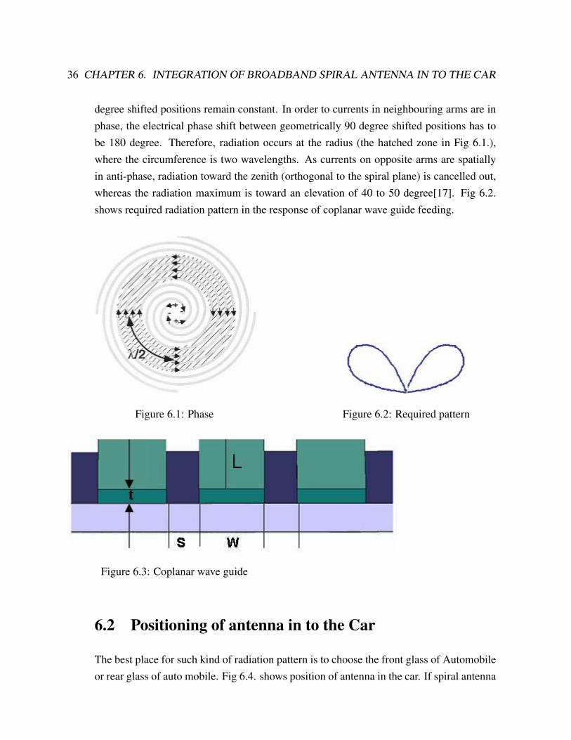
36 CHAPTER 6. INTEGRATION OF BROADBAND SPIRAL ANTENNA IN TO THE CAR
degree shifted positions remain constant. In order to currents in neighbouring arms are inphase, the electrical phase shift between geometrically 90 degree shifted positions has tobe 180 degree. Therefore, radiation occurs at the radius (the hatched zone in Fig 6.1.),where the circumference is two wavelengths. As currents on opposite arms are spatiallyin anti-phase, radiation toward the zenith (orthogonal to the spiral plane) is cancelled out,whereas the radiation maximum is toward an elevation of 40 to 50 degree[17]. Fig 6.2.shows required radiation pattern in the response of coplanar wave guide feeding.
Figure 6.1: Phase Figure 6.2: Required pattern
Figure 6.3: Coplanar wave guide
6.2 Positioning of antenna in to the Car
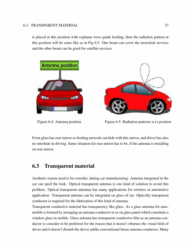
The best place for such kind of radiation pattern is to choose the front glass of Automobileor rear glass of auto mobile. Fig 6.4. shows position of antenna in the car. If spiral antenna
6.3. TRANSPARENT MATERIAL 37
is placed at this position with coplanar wave guide feeding, then the radiation pattern atthis position will be same like as in Fig 6.5. One beam can cover the terrestrial servicesand the other beam can be good for satellite services.
Figure 6.4: Antenna position Figure 6.5: Radiation patteren w.r.t position
Front glass has rear mirror so feeding network can hide with this mirror, and driver has alsono interlude in driving. Same situation for rear mirror has to be, if the antenna is installingon rear mirror.
6.3 Transparent material
Aesthetic reason need to be consider, during car manufacturing. Antenna integrated in thecar can spoil the look. Optical transparent antenna is one kind of solution to avoid thisproblem. Optical transparent antennas has many applications for wireless or automotiveapplication. Transparent antenna can be integrated on glass of car. Optically transparentconductor is required for the fabrication of this kind of antenna.Transparent conductive material has transparency like glass. As a glass antenna for auto-mobile is formed by arranging an antenna conductor in or on glass panel which constitute awindow glass in mobile. Glass antenna has transparent conductive film as an antenna con-ductor is consider to be preferred for the reason that it doesn’t obstruct the visual field ofdriver and it doesn’t disturb the driver unlike conventional linear antenna conductor. Many
38 CHAPTER 6. INTEGRATION OF BROADBAND SPIRAL ANTENNA IN TO THE CAR
transparent conductive materials are available, which can be used for antenna design.ITO (Indium tin oxide) is a conductive transparent material which can work for antenna.It has low sheet resistivity and the high transparency. Due to high cost of this material wewill not include it in this project.Generally polymers are called insulator. However there is a special class of polymers-theintrinsically conductive polymers-that have conductivity levels between those of semicon-ductor and metal. Such kind of combination is completely new in electronic industry. Thismaterial can help in many electronic projects.
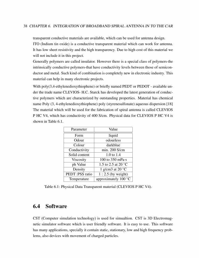
With poly(3,4-ethylenedioxythiophene) or briefly named PEDT or PEDOT - available un-der the trade name CLEVIOS- H.C. Starck has developed the latest generation of conduc-tive polymers which are characterized by outstanding properties. Material has chemicalname Poly (3, 4-ethylenedioxythiophene) poly (styrenesulfonate) aqueous dispersion [18]The material which will be used for the fabrication of spiral antenna is called CLEVIOSP HC V4, which has conductivity of 400 S/cm. Physical data for CLEVIOS P HC V4 isshown in Table 6.1.
Parameter Value
Form liquidOdour odourlessColour darkblue
Conductivity min. 200 S/cmSolid content 1.0 to 1.4
Viscosity 100 to 350 mPa·sph Value 1.5 to 2.5 at 20 CDensity 1 g/cm3 at 20 C
PEDT :PSS ratio 1 : 2.5 (by weight)Temperature approximately 100 C
Table 6.1: Physical Data Transparent material (CLEVIOS P HC V4).
6.4 Software
CST (Computer simulation technology) is used for simualtion. CST is 3D Electromag-netic simulator software which is user friendly software. It is easy to use. This softwarehas many applications, specially it contain static, stationary, low and high frequency prob-lems, also devices with movement of charged particles.
6.5. PREVIOUS WORK 39
6.5 Previous Work
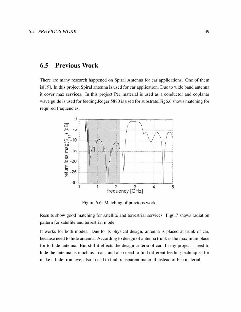
There are many research happened on Spiral Antenna for car applications. One of themis[19]. In this project Spiral antenna is used for car application. Due to wide band antennait cover max services. In this project Pec material is used as a conductor and coplanarwave guide is used for feeding.Roger 5880 is used for substrate.Fig6.6 shows matching forrequired frequencies.
Figure 6.6: Matching of previous work
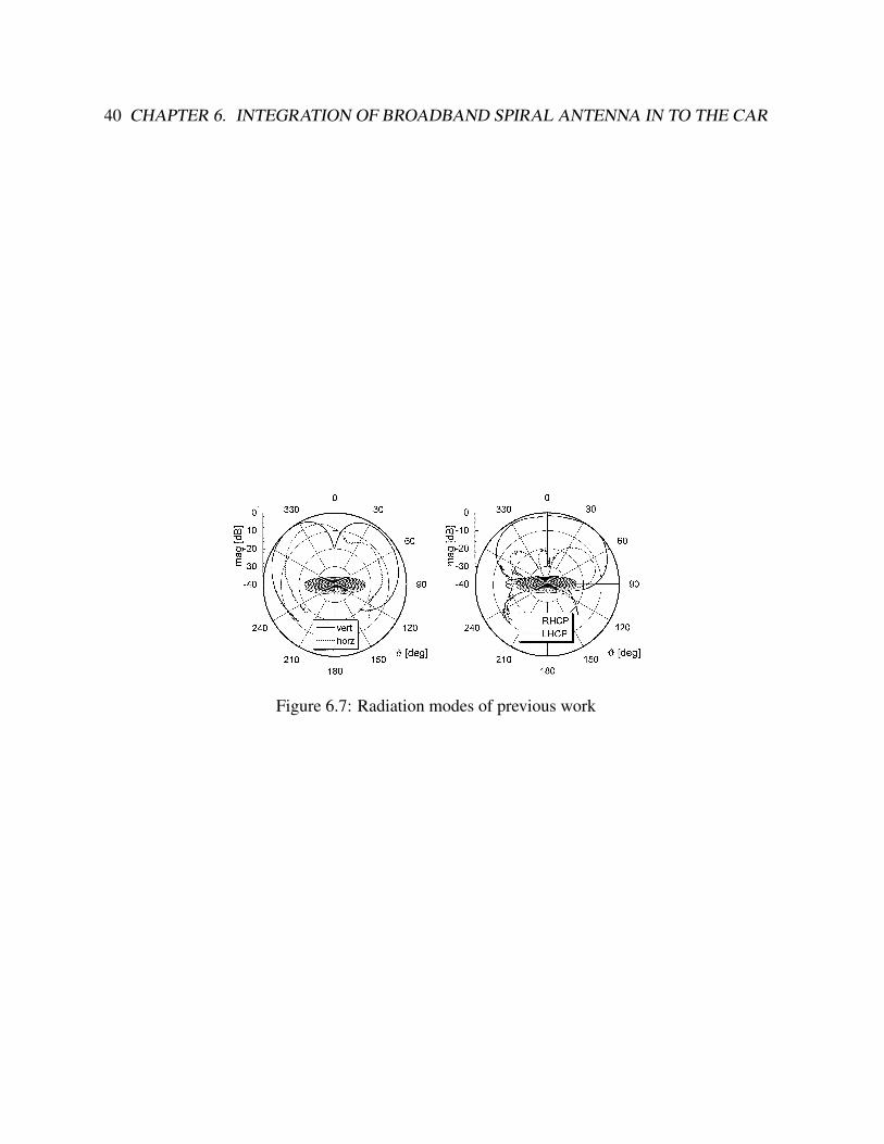
Results show good matching for satellite and terrestrial services. Fig6.7 shows radiationpattern for satellite and terrestrial mode.
It works for both modes. Due to its physical design, antenna is placed at trunk of car,because need to hide antenna. According to design of antenna trunk is the maximum placefor to hide antenna. But still it effects the design criteria of car. In my project I need tohide the antenna as much as I can. and also need to find different feeding techniques formake it hide from eye, also I need to find transparent material instead of Pec material.
40 CHAPTER 6. INTEGRATION OF BROADBAND SPIRAL ANTENNA IN TO THE CAR
Figure 6.7: Radiation modes of previous work
Chapter 7
Results
In this chapter spiral antenna is designed with PEC material and CLEVIOS P HC V4conductive transparent material. Detail of this conductive transparent material is alreadydefined in previous chapter. Spiral antenna is integrated in front glass of vehicle whichmake it hygienic. Coplanar wave guide is used for feeding antenna.
7.1 Four-Arm Spiral antenna PEC material centre feed-ing
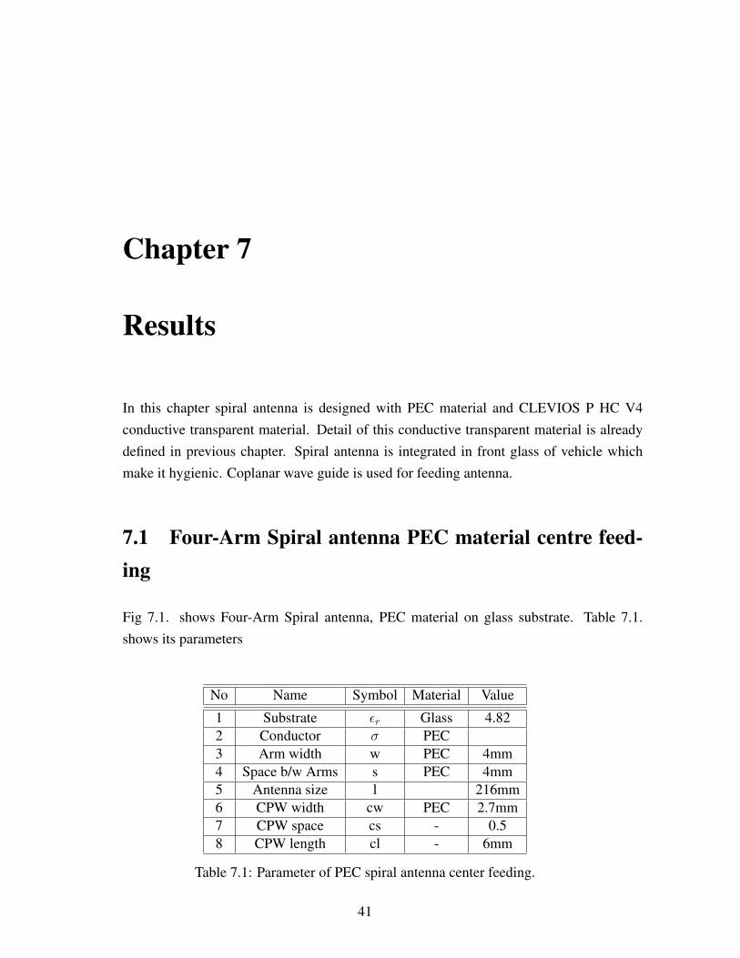
Fig 7.1. shows Four-Arm Spiral antenna, PEC material on glass substrate. Table 7.1.shows its parameters
No Name Symbol Material Value
1 Substrate εr Glass 4.822 Conductor σ PEC3 Arm width w PEC 4mm4 Space b/w Arms s PEC 4mm5 Antenna size l 216mm6 CPW width cw PEC 2.7mm7 CPW space cs - 0.58 CPW length cl - 6mm
Table 7.1: Parameter of PEC spiral antenna center feeding.
41
42 CHAPTER 7. RESULTS
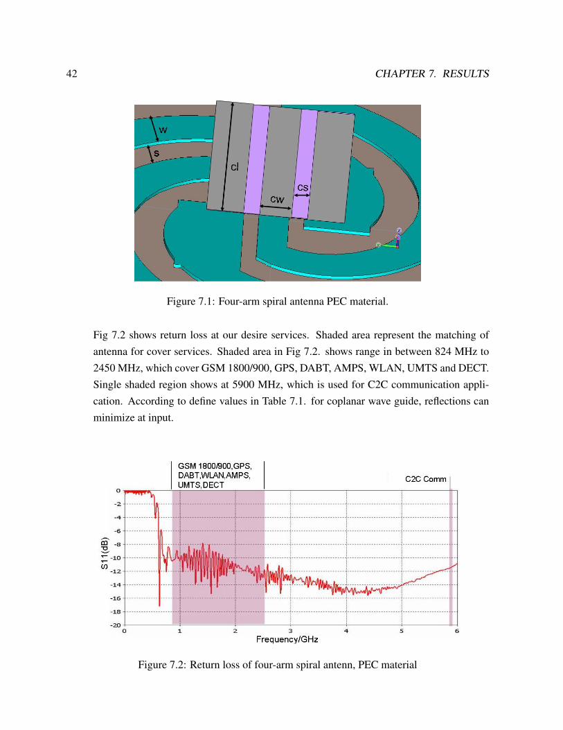
Figure 7.1: Four-arm spiral antenna PEC material.
Fig 7.2 shows return loss at our desire services. Shaded area represent the matching ofantenna for cover services. Shaded area in Fig 7.2. shows range in between 824 MHz to2450 MHz, which cover GSM 1800/900, GPS, DABT, AMPS, WLAN, UMTS and DECT.Single shaded region shows at 5900 MHz, which is used for C2C communication appli-cation. According to define values in Table 7.1. for coplanar wave guide, reflections canminimize at input.
Figure 7.2: Return loss of four-arm spiral antenn, PEC material
7.1. FOUR-ARM SPIRAL ANTENNA PEC MATERIAL CENTRE FEEDING 43
7.1.1 Radiation pattern
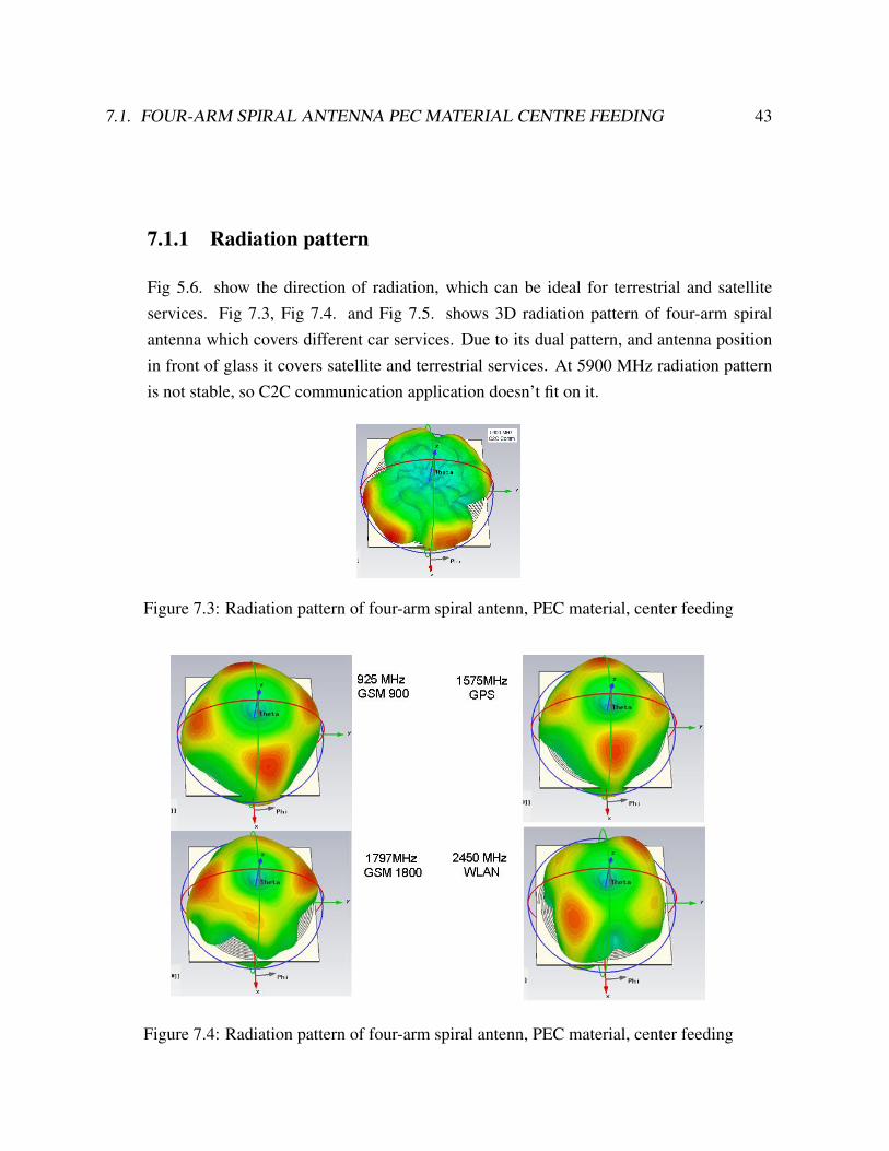
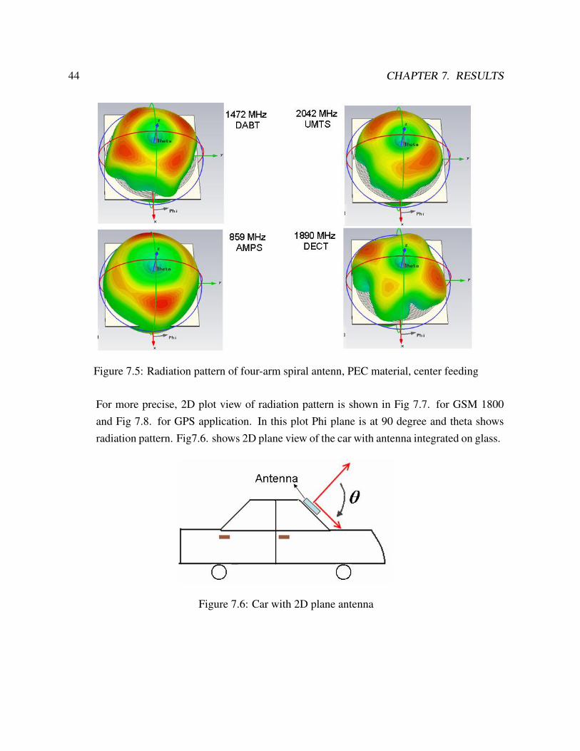
Fig 5.6. show the direction of radiation, which can be ideal for terrestrial and satelliteservices. Fig 7.3, Fig 7.4. and Fig 7.5. shows 3D radiation pattern of four-arm spiralantenna which covers different car services. Due to its dual pattern, and antenna positionin front of glass it covers satellite and terrestrial services. At 5900 MHz radiation patternis not stable, so C2C communication application doesn’t fit on it.
Figure 7.3: Radiation pattern of four-arm spiral antenn, PEC material, center feeding
Figure 7.4: Radiation pattern of four-arm spiral antenn, PEC material, center feeding
44 CHAPTER 7. RESULTS
Figure 7.5: Radiation pattern of four-arm spiral antenn, PEC material, center feeding
For more precise, 2D plot view of radiation pattern is shown in Fig 7.7. for GSM 1800and Fig 7.8. for GPS application. In this plot Phi plane is at 90 degree and theta showsradiation pattern. Fig7.6. shows 2D plane view of the car with antenna integrated on glass.
Figure 7.6: Car with 2D plane antenna
7.1. FOUR-ARM SPIRAL ANTENNA PEC MATERIAL CENTRE FEEDING 45
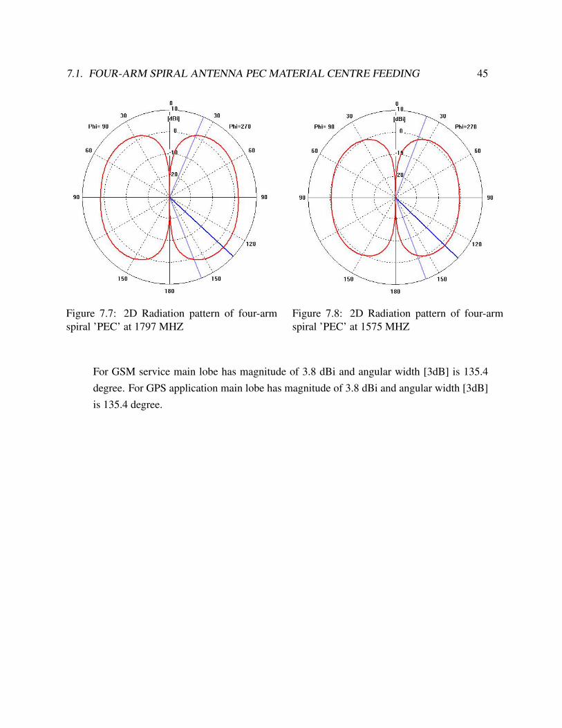
Figure 7.7: 2D Radiation pattern of four-armspiral ’PEC’ at 1797 MHZ
Figure 7.8: 2D Radiation pattern of four-armspiral ’PEC’ at 1575 MHZ
For GSM service main lobe has magnitude of 3.8 dBi and angular width [3dB] is 135.4degree. For GPS application main lobe has magnitude of 3.8 dBi and angular width [3dB]is 135.4 degree.
46 CHAPTER 7. RESULTS
7.2 Four-Arm Spiral antenna Transparent material cen-ter feeding
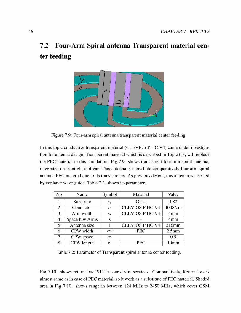
Figure 7.9: Four-arm spiral antenna transparent material center feeding.
In this topic conductive transparent material (CLEVIOS P HC V4) came under investiga-tion for antenna design. Transparent material which is described in Topic 6.3, will replacethe PEC material in this simulation. Fig 7.9. shows transparent four-arm spiral antenna,integrated on front glass of car. This antenna is more hide comparatively four-arm spiralantenna PEC material due to its transparency. As previous design, this antenna is also fedby coplanar wave guide. Table 7.2. shows its parameters.
No Name Symbol Material Value
1 Substrate εr Glass 4.822 Conductor σ CLEVIOS P HC V4 400S/cm3 Arm width w CLEVIOS P HC V4 4mm4 Space b/w Arms s - 4mm5 Antenna size l CLEVIOS P HC V4 216mm6 CPW width cw PEC 2.5mm7 CPW space cs - 0.58 CPW length cl PEC 10mm
Table 7.2: Parameter of Transparent spiral antenna center feeding.
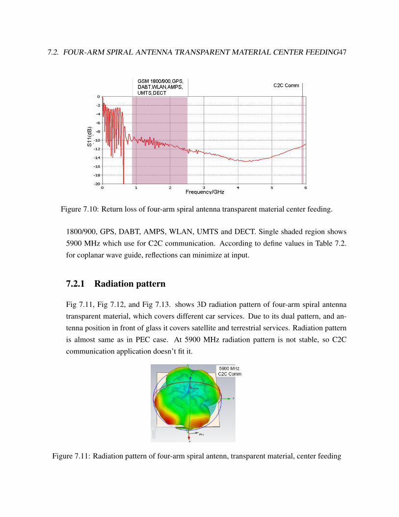
Fig 7.10. shows return loss ’S11’ at our desire services. Comparatively, Return loss isalmost same as in case of PEC material, so it work as a substitute of PEC material. Shadedarea in Fig 7.10. shows range in between 824 MHz to 2450 MHz, which cover GSM
7.2. FOUR-ARM SPIRAL ANTENNA TRANSPARENT MATERIAL CENTER FEEDING47
Figure 7.10: Return loss of four-arm spiral antenna transparent material center feeding.
1800/900, GPS, DABT, AMPS, WLAN, UMTS and DECT. Single shaded region shows5900 MHz which use for C2C communication. According to define values in Table 7.2.for coplanar wave guide, reflections can minimize at input.
7.2.1 Radiation pattern
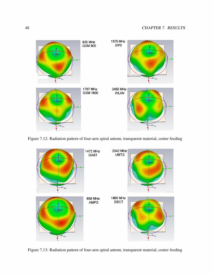
Fig 7.11, Fig 7.12, and Fig 7.13. shows 3D radiation pattern of four-arm spiral antennatransparent material, which covers different car services. Due to its dual pattern, and an-tenna position in front of glass it covers satellite and terrestrial services. Radiation patternis almost same as in PEC case. At 5900 MHz radiation pattern is not stable, so C2Ccommunication application doesn’t fit it.
Figure 7.11: Radiation pattern of four-arm spiral antenn, transparent material, center feeding
48 CHAPTER 7. RESULTS
Figure 7.12: Radiation pattern of four-arm spiral antenn, transparent material, center feeding
Figure 7.13: Radiation pattern of four-arm spiral antenn, transparent material, center feeding
7.2. FOUR-ARM SPIRAL ANTENNA TRANSPARENT MATERIAL CENTER FEEDING49
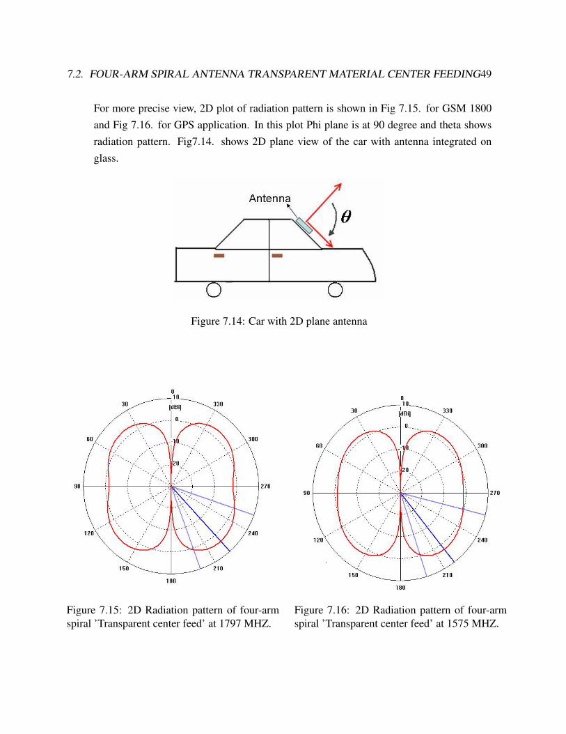
For more precise view, 2D plot of radiation pattern is shown in Fig 7.15. for GSM 1800and Fig 7.16. for GPS application. In this plot Phi plane is at 90 degree and theta showsradiation pattern. Fig7.14. shows 2D plane view of the car with antenna integrated onglass.
Figure 7.14: Car with 2D plane antenna
Figure 7.15: 2D Radiation pattern of four-armspiral ’Transparent center feed’ at 1797 MHZ.
Figure 7.16: 2D Radiation pattern of four-armspiral ’Transparent center feed’ at 1575 MHZ.
50 CHAPTER 7. RESULTS
For GSM service main lobe has magnitude of 3.7 dBi and angular width [3dB] is 51 de-gree. For GPS application main lobe has magnitude of 2.5 dBi and angular width [3dB] is57.6 degree.
7.3 Four-Arm Spiral antenna Transparent material backside feeding
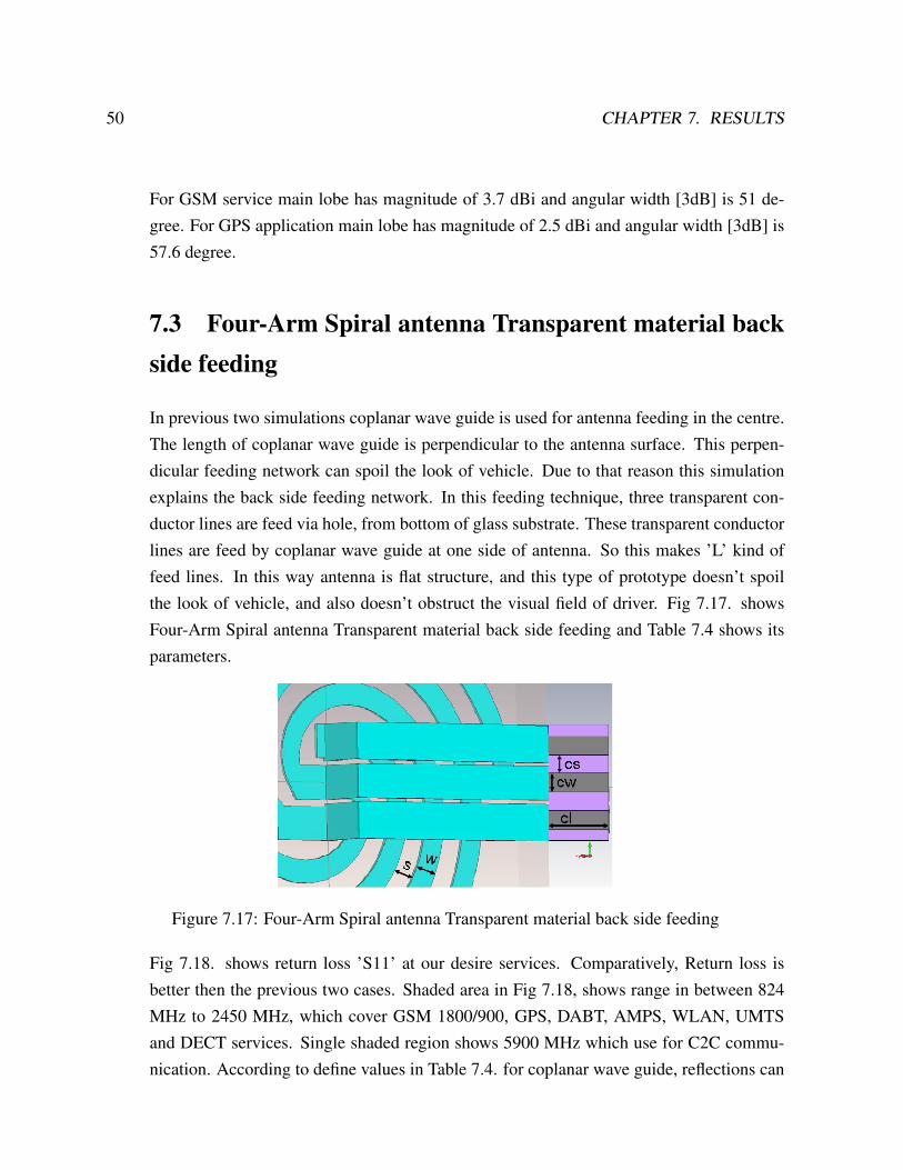
In previous two simulations coplanar wave guide is used for antenna feeding in the centre.The length of coplanar wave guide is perpendicular to the antenna surface. This perpen-dicular feeding network can spoil the look of vehicle. Due to that reason this simulationexplains the back side feeding network. In this feeding technique, three transparent con-ductor lines are feed via hole, from bottom of glass substrate. These transparent conductorlines are feed by coplanar wave guide at one side of antenna. So this makes ’L’ kind offeed lines. In this way antenna is flat structure, and this type of prototype doesn’t spoilthe look of vehicle, and also doesn’t obstruct the visual field of driver. Fig 7.17. showsFour-Arm Spiral antenna Transparent material back side feeding and Table 7.4 shows itsparameters.
Figure 7.17: Four-Arm Spiral antenna Transparent material back side feeding
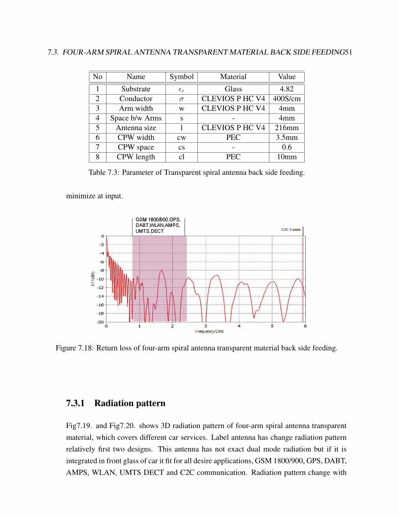
Fig 7.18. shows return loss ’S11’ at our desire services. Comparatively, Return loss isbetter then the previous two cases. Shaded area in Fig 7.18, shows range in between 824MHz to 2450 MHz, which cover GSM 1800/900, GPS, DABT, AMPS, WLAN, UMTSand DECT services. Single shaded region shows 5900 MHz which use for C2C commu-nication. According to define values in Table 7.4. for coplanar wave guide, reflections can
7.3. FOUR-ARM SPIRAL ANTENNA TRANSPARENT MATERIAL BACK SIDE FEEDING51
No Name Symbol Material Value
1 Substrate εr Glass 4.822 Conductor σ CLEVIOS P HC V4 400S/cm3 Arm width w CLEVIOS P HC V4 4mm4 Space b/w Arms s - 4mm5 Antenna size l CLEVIOS P HC V4 216mm6 CPW width cw PEC 3.5mm7 CPW space cs - 0.68 CPW length cl PEC 10mm
Table 7.3: Parameter of Transparent spiral antenna back side feeding.
minimize at input.
Figure 7.18: Return loss of four-arm spiral antenna transparent material back side feeding.
7.3.1 Radiation pattern
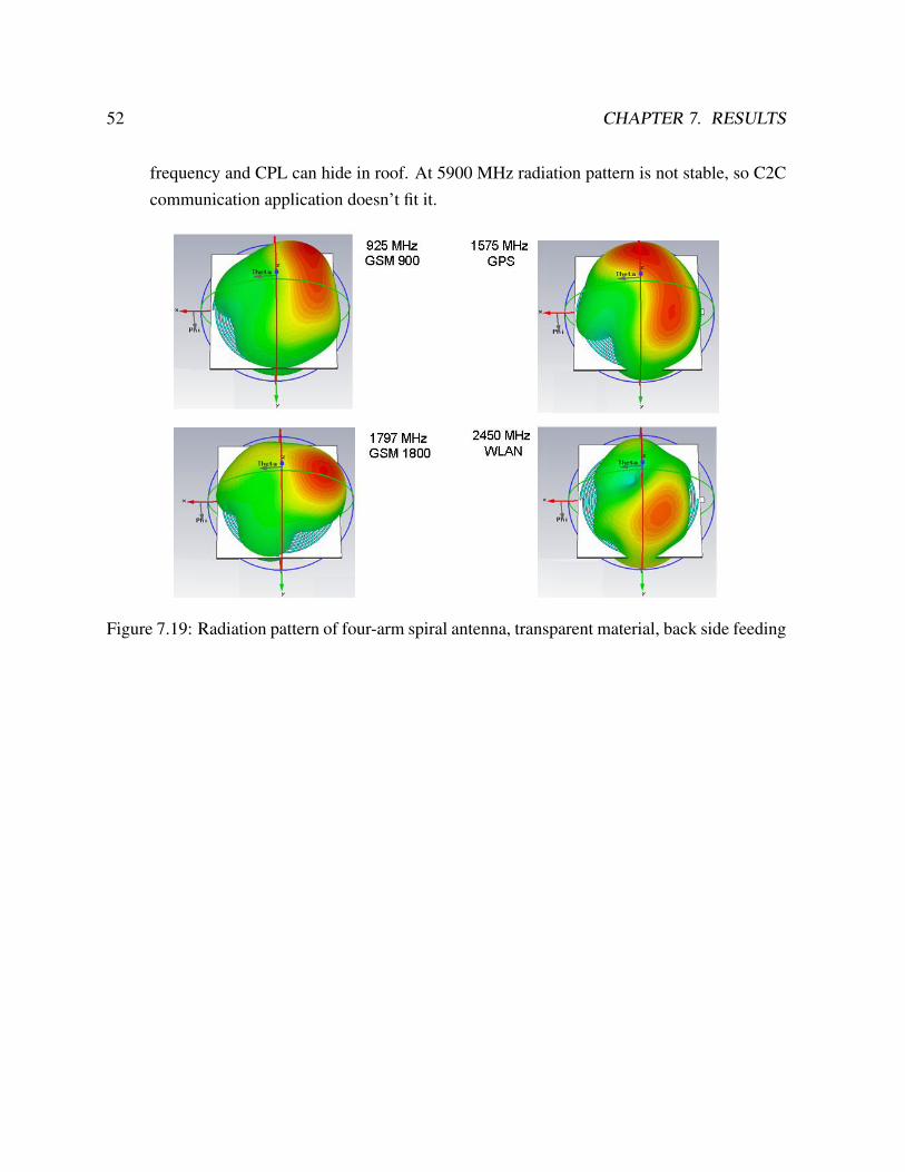
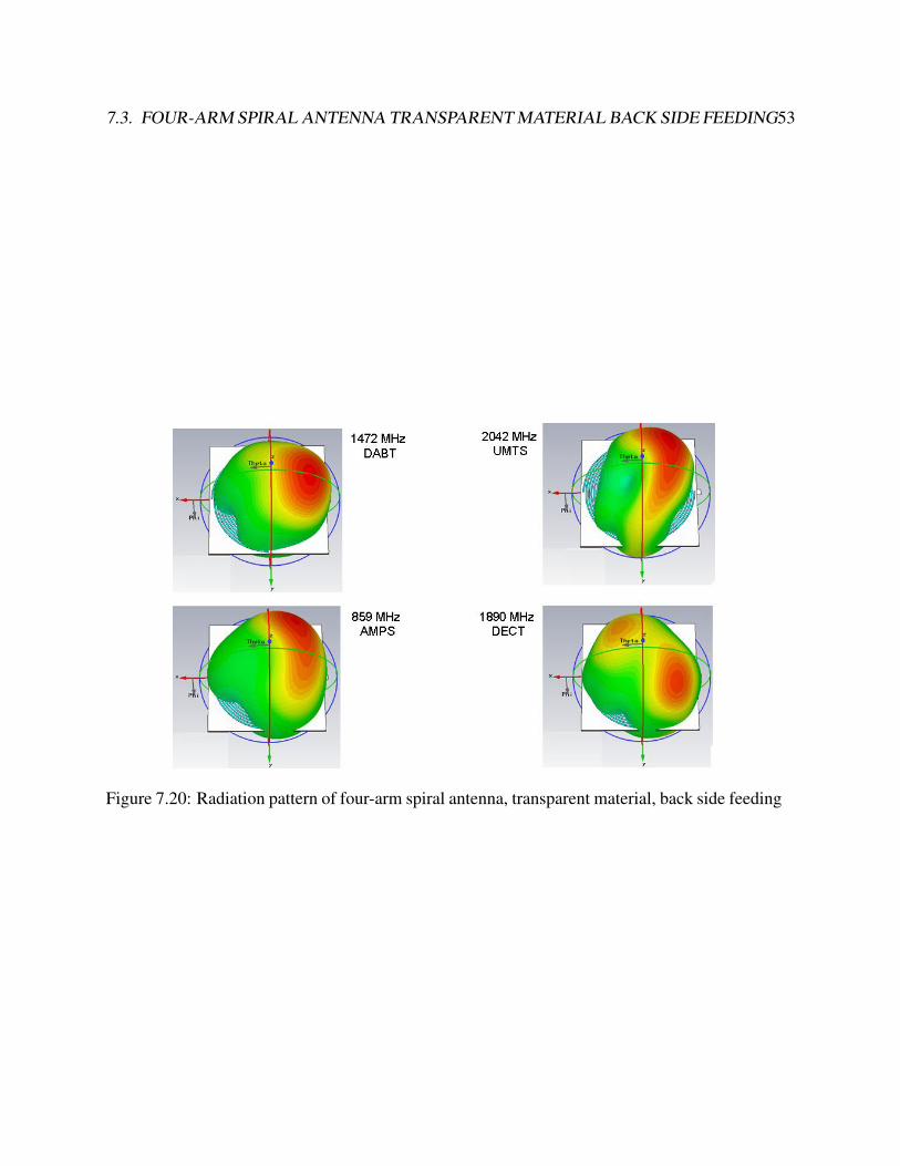
Fig7.19. and Fig7.20. shows 3D radiation pattern of four-arm spiral antenna transparentmaterial, which covers different car services. Label antenna has change radiation patternrelatively first two designs. This antenna has not exact dual mode radiation but if it isintegrated in front glass of car it fit for all desire applications, GSM 1800/900, GPS, DABT,AMPS, WLAN, UMTS DECT and C2C communication. Radiation pattern change with
52 CHAPTER 7. RESULTS
frequency and CPL can hide in roof. At 5900 MHz radiation pattern is not stable, so C2Ccommunication application doesn’t fit it.
Figure 7.19: Radiation pattern of four-arm spiral antenna, transparent material, back side feeding
7.3. FOUR-ARM SPIRAL ANTENNA TRANSPARENT MATERIAL BACK SIDE FEEDING53
Figure 7.20: Radiation pattern of four-arm spiral antenna, transparent material, back side feeding
54 CHAPTER 7. RESULTS
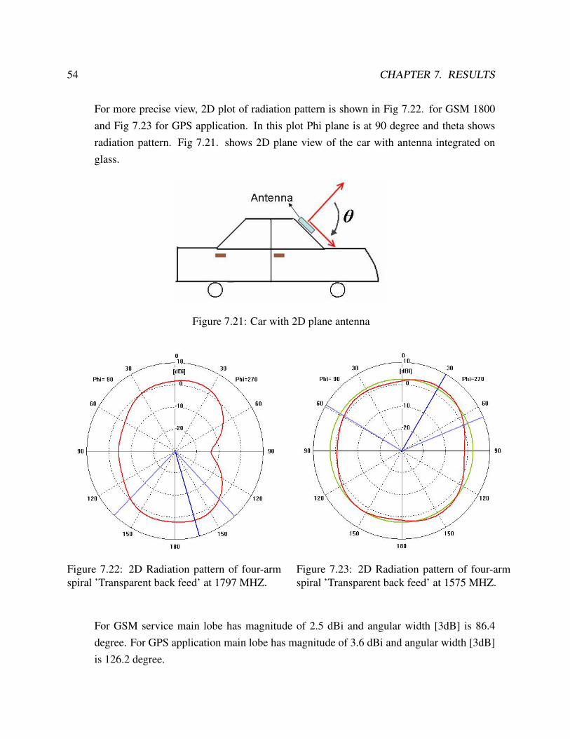
For more precise view, 2D plot of radiation pattern is shown in Fig 7.22. for GSM 1800and Fig 7.23 for GPS application. In this plot Phi plane is at 90 degree and theta showsradiation pattern. Fig 7.21. shows 2D plane view of the car with antenna integrated onglass.
Figure 7.21: Car with 2D plane antenna
Figure 7.22: 2D Radiation pattern of four-armspiral ’Transparent back feed’ at 1797 MHZ.
Figure 7.23: 2D Radiation pattern of four-armspiral ’Transparent back feed’ at 1575 MHZ.
For GSM service main lobe has magnitude of 2.5 dBi and angular width [3dB] is 86.4degree. For GPS application main lobe has magnitude of 3.6 dBi and angular width [3dB]is 126.2 degree.
7.4. TWO-ARM SPIRAL ANTENNA TP MATERIAL SIDE FEEDING 55
7.4 Two-Arm Spiral antenna TP material side feeding
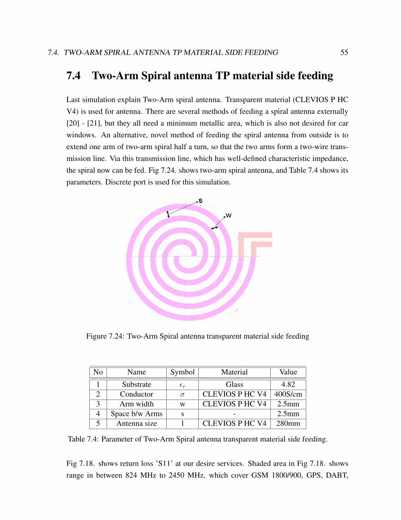
Last simulation explain Two-Arm spiral antenna. Transparent material (CLEVIOS P HCV4) is used for antenna. There are several methods of feeding a spiral antenna externally[20] - [21], but they all need a minimum metallic area, which is also not desired for carwindows. An alternative, novel method of feeding the spiral antenna from outside is toextend one arm of two-arm spiral half a turn, so that the two arms form a two-wire trans-mission line. Via this transmission line, which has well-defined characteristic impedance,the spiral now can be fed. Fig 7.24. shows two-arm spiral antenna, and Table 7.4 shows itsparameters. Discrete port is used for this simulation.
Figure 7.24: Two-Arm Spiral antenna transparent material side feeding
No Name Symbol Material Value
1 Substrate εr Glass 4.822 Conductor σ CLEVIOS P HC V4 400S/cm3 Arm width w CLEVIOS P HC V4 2.5mm4 Space b/w Arms s - 2.5mm5 Antenna size l CLEVIOS P HC V4 280mm
Table 7.4: Parameter of Two-Arm Spiral antenna transparent material side feeding.
Fig 7.18. shows return loss ’S11’ at our desire services. Shaded area in Fig 7.18. showsrange in between 824 MHz to 2450 MHz, which cover GSM 1800/900, GPS, DABT,
56 CHAPTER 7. RESULTS
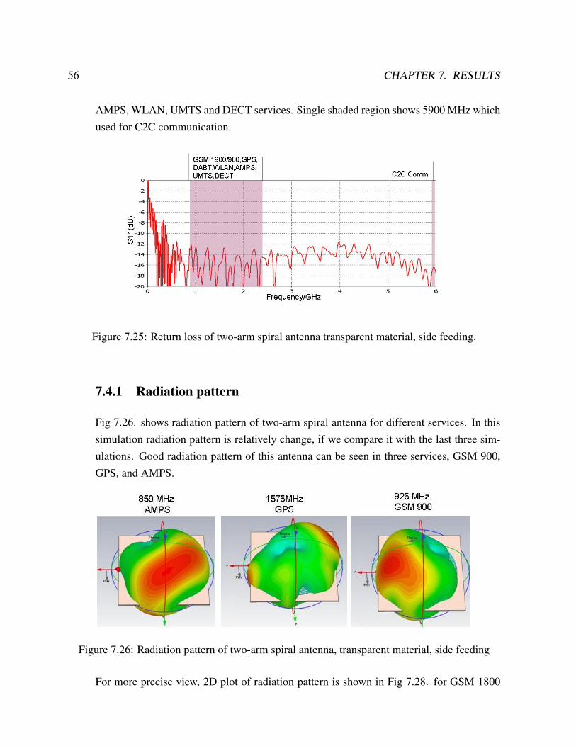
AMPS, WLAN, UMTS and DECT services. Single shaded region shows 5900 MHz whichused for C2C communication.
Figure 7.25: Return loss of two-arm spiral antenna transparent material, side feeding.
7.4.1 Radiation pattern
Fig 7.26. shows radiation pattern of two-arm spiral antenna for different services. In thissimulation radiation pattern is relatively change, if we compare it with the last three sim-ulations. Good radiation pattern of this antenna can be seen in three services, GSM 900,GPS, and AMPS.
Figure 7.26: Radiation pattern of two-arm spiral antenna, transparent material, side feeding
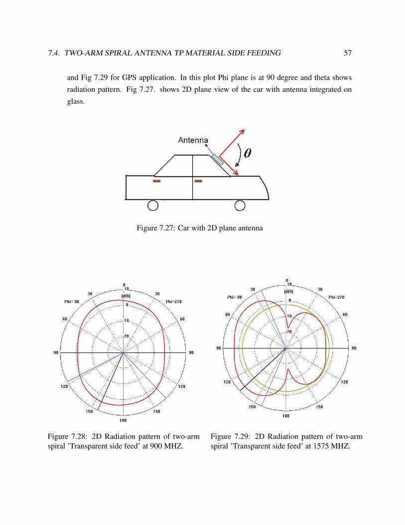
For more precise view, 2D plot of radiation pattern is shown in Fig 7.28. for GSM 1800
7.4. TWO-ARM SPIRAL ANTENNA TP MATERIAL SIDE FEEDING 57
and Fig 7.29 for GPS application. In this plot Phi plane is at 90 degree and theta showsradiation pattern. Fig 7.27. shows 2D plane view of the car with antenna integrated onglass.
Figure 7.27: Car with 2D plane antenna
Figure 7.28: 2D Radiation pattern of two-armspiral ’Transparent side feed’ at 900 MHZ.
Figure 7.29: 2D Radiation pattern of two-armspiral ’Transparent side feed’ at 1575 MHZ.
58 CHAPTER 7. RESULTS
For GSM service main lobe has magnitude of 4.2 dBi and angular width [3dB] is 105.6degree. For GPS application main lobe has magnitude of 5.8 dBi and angular width [3dB]is 133.7 degree.
7.5 Comparison
Spiral antenna is used in many applications, due to its wide band characteristics. There aremany research happened on Spiral antenna for the car applications. Past research is mostlybased on PEC conductive material and Roger 5880 is used as a substrate. One of researchhas Four arm spiral antenna with coplanar wave guide feeding for car[19]. Antenna givesbetter matching for both satellite and terrestial services.The return loss for the terrestrialmode is better than -10dB from 670 MHz to over 5 GHz.This shows large input impedancebandwidth obtainable with this antenna.The return loss for the satellite mode is better than-10dB in the range from 1.3 GHz up to 2.2 GHz.So satellite services also can be coveredin a broadband wayMain idea in this project is to replace the PEC material with transparent conductive mate-rial, and glass is used as a substrate. All simulations in this Project has return loss better-10dB for both satellite and terrestrial services. but comparatively previous work, thisproject has less matching due to low conductivity of transparent material. Four-Arm Spi-ral antenna transparent material back side feeding has return loss better then -10dB in therange from 1 GHz to 1.6 GHz, which cover satellite service. Return loss for terrestrialservices is also better then -10 dB in the range from 800 MHz to 5.9 GHz with exceptionsof -8dB for some points.
Chapter 8
Conclusion and Future Analysis
8.1 Conclusion
In order to make a final conclusion about the best performing antenna position for C2Ccommunications is under the car. Several aspects have to be taken into account, like thedesign considerations. Also a summary of each analyzed parameter will be done. Designconsiderations have to be taken into consideration also, as this will be very important inthe implementation of the antenna. As there are some positions at the car, which are notso easy to locate an antenna. Antenna under the car can be safe. At the bottom of the car,there are no design restrictions and the designers will not have so many problems to locatea communication system device here. In Scenarios, LOS and NLOS antenna is placedunder the car and urban environment is defined in simulation.For LOS and NLOS case long-term fading is shown in Fig3.2 and Fig3.5. Signal lossescan be seen at different points. NLOS shows less path loss comparatively LOS, it can gofor NLOS case because no vehicle is moving parallel with both cars. But for LOS casesome cars are moving parallel to both. For NLOS case one vehicle is in between both cars,it can make constructive signal at receiver side due to its reflection.
Short-term fading component can distinguish between LOS and NLOS case. For LOS casedeviation from 0 dB is large. In this case rapid fluctuation can be seen and it has probabil-ity to lost the data. But for NLOS case deviation from 0 dB is not so large. So it has morechances to get signal at receiver.Measurement results are morels same like NLOS case, due to maximum time, some ve-hicles in between. Path loss reached maximum 88 dB which was the worse case and
59
60 CHAPTER 8. CONCLUSION AND FUTURE ANALYSIS
minimum path loss obtains 70 dB. Monopole antenna is not radiating exact in omni pat-tern. Radiation pattern is bended toward the earth, so signal can reach at receiver afterground reflection, this factor plays vital role in measurements. Earth surface is not smoothlike we had consider in ray tracing simulation so fraction of earth surface is also involvedin measurements.Different kind of broad band antennas are discussed. Some of them are rejected due tothere radiation pattern and structure. Spiral antenna can work for multitude radio servicesand can help for automotive applications. Four-arm spiral fed with a coplanar transmis-sion line, in the response both terrestrial services and satellite services covers. Position forantenna in the car is important consideration, and I had found that front glass of car, worksbetter for dual mode radiation. Radiation can be seen at both side of antenna, so if antennais integrated inside the car, still it can work.Simulations shows that transparent conductive material has good approach for automotiveapplication, like PEC material. Four-arm spiral antenna feed through back side can alsowork for automotive and all necessary services can cover by this. Integration of Four-armspiral antenna feed through back side is easy to integrate on glass.Two-arm spiral antenna which is intended to be integrated in the front glass of car. The pro-posed novel external feeding structure allows feed this antenna frequency-independently.The pattern change with frequency and is reliant on the location on the car. Due to highgain it has edge compare to other simulations.
8.2 Future Analysis
In this project work two scenarios are set and then analyze different channel characteris-tics. Scenario is based on measurement track. It will be very interesting to have the resultsand conclusions for other scenarios and measurements. Urban scenario is used for thisproject, motorway scenario and measurements could be interesting.In this project monopole antenna is used under the car but some other antennas can also beanalyzed with different radiation pattern. Finally, it will be important to analyze diversity-systems. In order to combine different antenna positions as transmitters or receivers. Theresults will be better, as if an antenna position is not performing so well in a certain mo-ment, if there is another antenna located in another position at the car, this will improvethe behaviour of the whole systemSecond part is based on broad band antenna with PEC and transparent material. It is based
8.2. FUTURE ANALYSIS 61
on simulations, so it could be more interesting if prototype is installing on the car and thenanalyze the radiation pattern. Also some other positions for antenna on the car can be ana-lyze. In this project work the analysis is done in front glass of car for antenna integration,so another interesting improvement will be to analyze other position of car for antennaintegration. Irregular radiation problem at 5.9 GHz frequency can be fixed in future work.Some other broad band antennas can also be used for analyzing transparent material.

62 CHAPTER 8. CONCLUSION AND FUTURE ANALYSIS

List of Figures
1.1 Block Diagram of objective. . . . . . . . . . . . . . . . . . . . . . . . . 3
2.1 Long-term fading . . . . . . . . . . . . . . . . . . . . . . . . . . . . . . 6
2.2 Short-term fading . . . . . . . . . . . . . . . . . . . . . . . . . . . . . . 7
3.1 LOS Scenario . . . . . . . . . . . . . . . . . . . . . . . . . . . . . . . . 9
3.2 Long-term fading for LOS case. . . . . . . . . . . . . . . . . . . . . . . 10
3.3 Short-term fading for LOS case. . . . . . . . . . . . . . . . . . . . . . . 11
3.4 NLOS Scenario . . . . . . . . . . . . . . . . . . . . . . . . . . . . . . . 12
3.5 Long-term fading for NLOS case. . . . . . . . . . . . . . . . . . . . . . 13
3.6 Short-term fading for NLOS case. . . . . . . . . . . . . . . . . . . . . . 14
4.1 Possible position for antenna . . . . . . . . . . . . . . . . . . . . . . . . 15
4.2 Signal to noise ratio for different antenna positions. . . . . . . . . . . . . 16
4.3 Monopole antenna Radiation Pattern . . . . . . . . . . . . . . . . . . . . 17
4.4 Block diagram of measurment setup . . . . . . . . . . . . . . . . . . . . 17
4.5 Transmitter setup . . . . . . . . . . . . . . . . . . . . . . . . . . . . . . 18
4.6 Receiver setup . . . . . . . . . . . . . . . . . . . . . . . . . . . . . . . . 18
4.7 Measurement track . . . . . . . . . . . . . . . . . . . . . . . . . . . . . 19
4.8 Long term fading for measurment setup. . . . . . . . . . . . . . . . . . . 20
4.9 Short term fading for measurment setup. . . . . . . . . . . . . . . . . . . 21
63
64 LIST OF FIGURES
5.1 Rectangular plot of Radiation Pattern . . . . . . . . . . . . . . . . . . . . 24
5.2 linear vertical polarization . . . . . . . . . . . . . . . . . . . . . . . . . 25
5.3 linear horizontal polarization . . . . . . . . . . . . . . . . . . . . . . . . 25
5.4 Circular Polarization . . . . . . . . . . . . . . . . . . . . . . . . . . . . 26
5.5 Elliptical Polarization . . . . . . . . . . . . . . . . . . . . . . . . . . . . 26
5.6 Required Radiation pattern . . . . . . . . . . . . . . . . . . . . . . . . . 27
5.7 Vivaldi antenna . . . . . . . . . . . . . . . . . . . . . . . . . . . . . . . 28
5.8 Bowtie antenna . . . . . . . . . . . . . . . . . . . . . . . . . . . . . . . 29
5.9 Log-periodic antenna . . . . . . . . . . . . . . . . . . . . . . . . . . . . 30
5.10 Two-arm spiral antenna . . . . . . . . . . . . . . . . . . . . . . . . . . . 31
5.11 Four-arm spiral antenna . . . . . . . . . . . . . . . . . . . . . . . . . . . 31
5.12 Conical Spiral antenna . . . . . . . . . . . . . . . . . . . . . . . . . . . 31
6.1 Phase . . . . . . . . . . . . . . . . . . . . . . . . . . . . . . . . . . . . 36
6.2 Required pattern . . . . . . . . . . . . . . . . . . . . . . . . . . . . . . . 36
6.3 Coplanar wave guide . . . . . . . . . . . . . . . . . . . . . . . . . . . . 36
6.4 Antenna position . . . . . . . . . . . . . . . . . . . . . . . . . . . . . . 37
6.5 Radiation patteren w.r.t position . . . . . . . . . . . . . . . . . . . . . . 37
6.6 Matching of previous work . . . . . . . . . . . . . . . . . . . . . . . . . 39
6.7 Radiation modes of previous work . . . . . . . . . . . . . . . . . . . . . 40
7.1 Four-arm spiral antenna PEC material. . . . . . . . . . . . . . . . . . . . 42
7.2 Return loss of four-arm spiral antenn, PEC material . . . . . . . . . . . . 42
7.3 Radiation pattern of four-arm spiral antenn, PEC material, center feeding 43
7.4 Radiation pattern of four-arm spiral antenn, PEC material, center feeding 43
7.5 Radiation pattern of four-arm spiral antenn, PEC material, center feeding 44
7.6 Car with 2D plane antenna . . . . . . . . . . . . . . . . . . . . . . . . . 44
7.7 2D Radiation pattern of four-arm spiral ’PEC’ at 1797 MHZ . . . . . . . 45

LIST OF FIGURES 65
7.8 2D Radiation pattern of four-arm spiral ’PEC’ at 1575 MHZ . . . . . . . 45
7.9 Four-arm spiral antenna transparent material center feeding. . . . . . . . 46
7.10 Return loss of four-arm spiral antenna transparent material center feeding. 47
7.11 Radiation pattern of four-arm spiral antenn, transparent material, centerfeeding . . . . . . . . . . . . . . . . . . . . . . . . . . . . . . . . . . . 47
7.12 Radiation pattern of four-arm spiral antenn, transparent material, centerfeeding . . . . . . . . . . . . . . . . . . . . . . . . . . . . . . . . . . . 48
7.13 Radiation pattern of four-arm spiral antenn, transparent material, centerfeeding . . . . . . . . . . . . . . . . . . . . . . . . . . . . . . . . . . . 48
7.14 Car with 2D plane antenna . . . . . . . . . . . . . . . . . . . . . . . . . 49
7.15 2D Radiation pattern of four-arm spiral ’Transparent center feed’ at 1797MHZ. . . . . . . . . . . . . . . . . . . . . . . . . . . . . . . . . . . . . 49
7.16 2D Radiation pattern of four-arm spiral ’Transparent center feed’ at 1575MHZ. . . . . . . . . . . . . . . . . . . . . . . . . . . . . . . . . . . . . 49
7.17 Four-Arm Spiral antenna Transparent material back side feeding . . . . . 50
7.18 Return loss of four-arm spiral antenna transparent material back side feeding. 51
7.19 Radiation pattern of four-arm spiral antenna, transparent material, backside feeding . . . . . . . . . . . . . . . . . . . . . . . . . . . . . . . . . 52
7.20 Radiation pattern of four-arm spiral antenna, transparent material, backside feeding . . . . . . . . . . . . . . . . . . . . . . . . . . . . . . . . . 53
7.21 Car with 2D plane antenna . . . . . . . . . . . . . . . . . . . . . . . . . 54
7.22 2D Radiation pattern of four-arm spiral ’Transparent back feed’ at 1797MHZ. . . . . . . . . . . . . . . . . . . . . . . . . . . . . . . . . . . . . 54
7.23 2D Radiation pattern of four-arm spiral ’Transparent back feed’ at 1575MHZ. . . . . . . . . . . . . . . . . . . . . . . . . . . . . . . . . . . . . 54
7.24 Two-Arm Spiral antenna transparent material side feeding . . . . . . . . 55
7.25 Return loss of two-arm spiral antenna transparent material, side feeding. . 56
7.26 Radiation pattern of two-arm spiral antenna, transparent material, sidefeeding . . . . . . . . . . . . . . . . . . . . . . . . . . . . . . . . . . . 56
66 LIST OF FIGURES
7.27 Car with 2D plane antenna . . . . . . . . . . . . . . . . . . . . . . . . . 57
7.28 2D Radiation pattern of two-arm spiral ’Transparent side feed’ at 900MHZ. . . . . . . . . . . . . . . . . . . . . . . . . . . . . . . . . . . . . 57
7.29 2D Radiation pattern of two-arm spiral ’Transparent side feed’ at 1575 MHZ. 57
List of Tables
1.1 Different services and frequency bands. . . . . . . . . . . . . . . . . . . 2
6.1 Physical Data Transparent material (CLEVIOS P HC V4). . . . . . . . . 38
7.1 Parameter of PEC spiral antenna center feeding. . . . . . . . . . . . . . . 41
7.2 Parameter of Transparent spiral antenna center feeding. . . . . . . . . . . 46
7.3 Parameter of Transparent spiral antenna back side feeding. . . . . . . . . 51
7.4 Parameter of Two-Arm Spiral antenna transparent material side feeding. . 55
67

68 LIST OF TABLES
Bibliography [1] Car-to-Car communication, www.car-to-car.org/. [2] Itsaso Eizmendi, “Optimization of antenna placement for car-to-car communications
with ray-tracing”, Master Thesis, University of Karlsruhe, 2009 [3] Kelsey Mays, “BMW Studies Car-to-Car Communication”, http://blogs.cars.com,
2009. [4] Prepared by the IEEE 802.11 Working Group of the IEEE 802 Committee, “Draft
Standard for Information Technology, Telecommunications and information exchange between systems, Local and metropolitan area networks, Specific requirements, 2008.
[5] Geng Norbert, Wiesbeck Werner, “Planungsmethoden für die Mobilkommunication”, Book for Radio network planning in a real physical propagation conditions,
University of Karlsruhe, 1998. [6] A. Andujar, J. Anguera, and C. Puente, “ON THE RADIATION PATTERN OF THE
L-SHAPED WIRE ANTENNA” Technology and Intellectual Property Rights Department Fractus Barcelona, Spain, Research Paper, Vol 6, 2009
[7] Buon Kiong Lau Andersen, J.B. Molisch, A.F. Kristensson, G, “Antenna Matching
for Capacity Maximization in Compact MIMO Systems”, Lund University, IEEE paper, 2006
[8] Frc group, “Why Circular Polarization Antenna? ” http://www.frccorp.com/. [9] J. H. Shafieha, J. Noorinia, and Ch. Ghobadi, “PROBING THE FEED LINE
PARAMETERS IN VIVALDI NOTCH ANTENNAS”, Progress In Electromagnetics Research B, Vol. 1, 237–252, 2008
[10] Wang, H.Y. Mirshekar-Syahkal, D. Dilworth, I.J, “A rigorous analysis of tapered slot
antennas on dielectric substrates”, IEE paper, Antennas and Propagation, Tenth International Conference on (Conf. Publ. No. 436).1997
[11] Jen-Fen Huang , Chih-Wen Kuo, “CPW-fed bow-tie slot antenna”, Microwave and
optical technology letters, Volume 19 Issue 5, Pages 358 – 360, University, Kaohsiung, Taiwan, 1998.
[12] Hans Gregory Schantz, “A BRIEF HISTORY OF UWB ANTENNAS”, IEEE UWBST
Conference, 2003 [13] Dimitris E. Anagnostou, John Papapolymerou, Manos M. Tentzeris, Christos G.
Christodoulou, “BMW A Printed Log-Periodic Koch-Dipole Array (LPKDA)”, IEEE paper , ANTENNAS AND WIRELESS PROPAGATION LETTERS, VOL. 7, 2008 [14] Comprehensive EM solution, http://www.feko.info/ [15] Eric D. Caswell, “Design and Analysis of Star Spiral with Application to Wideband
Arrays with Variable Element Sizes”, Virginia Polytechnic Institute and State University PHD Thesis, 2001.
[16] Riaziat, M.; Majidi-Ahy, R.; Feng, I.-J, “Propagation modes and dispersion
characteristics of coplanar waveguides”, Microwave Theory and Techniques, IEEE Transactions on Volume 38, Page(s):245 – 251, 1990
[17] Gschwendtner, E.; Wiesbeck, W, “Ultra-broadband car antennas for communications
and navigation applications”, Antennas and Propagation, IEEE Transactions on Volume 51, Issue 8, Page(s): 2020 – 2027, 2003
[18] S. kirchmeyer, l. brassat, http://www.clevios.com. [19] Gschwendtner, E.; Wiesbeck, W, “Ultra-broadband car antennas for communications
and navigation applications”, Antennas and Propagation, IEEE Transactions on Volume 51, Issue 8, Page(s): 2020 – 2027, 2003
[20] Dr.-Ing. W. Wiesbeck, “ Ultra breitbandige Antennen f¨ur Kommunikation und
Navigation am Fahrzeug”, Wellenausbreitung und Planung digitaler Netze, Research paper.University of Karlsruhe
[21] Hisamatsu Nakano, Shigeru Okuzawa , Hiroaki Mimaki, “Two-arm slot spiral
antenna”,Article, Publisher: Taylor & Francis , Volume 14, , pages 397 – 413, 1994.