Master's Thesis- Developed by team at University of - Diabetes ...
MASTER'S THESIS
Image Processing Software developed with
MATLAB®
(Graphic Design Software - GDS)
Study: Master in Electronic Engineering (MEE)
Author: Llorenç Guerrero Pueyo
Director: Antoni Gasull
Year: 2015

Image Processing Software Developed With MATLAB® 1
Index
Index ........................................................................................... 1
Collaborations ............................................................................... 4
Thanks ......................................................................................... 5
Resum del Projecte ........................................................................ 6
Resumen del Proyecto ................................................................... 7
Abstract ....................................................................................... 8
1. Introduction........................................................................... 9
1.1 Context of the project .......................................................... 9
1.2 Objectives ......................................................................... 10
1.3 Structure of the report ....................................................... 12
2. GDS; main features .............................................................. 13
2.1 App development with MATLAB® GUIDE ............................... 13
2.2 Graphic Design Software - general overview of the application 16
2.2.1 Application window .......................................................... 16
2.2.2 Apps interaction .............................................................. 19
2.3 Image Processing Tools ...................................................... 20
2.3.1 Toolbar .......................................................................... 20
Open Image .......................................................................... 21
Image Information ................................................................. 22
RGB to gray .......................................................................... 23
Binary Threshold ................................................................... 23
Erode & Dilate Image ............................................................. 24
Horizontal & Vertical Flip ......................................................... 28
Cylinder & Sphere Deformation ............................................... 28
Image Profile ........................................................................ 30
Histogram ............................................................................. 31
Rotation ............................................................................... 32
2 Image Processing Software Developed With MATLAB®
Resize .................................................................................. 33
Crop .................................................................................... 33
Brightness ............................................................................ 34
Auto Contrast ........................................................................ 35
Geometrical shapes ................................................................ 36
Invert Image ......................................................................... 37
Stitch Images ........................................................................ 38
Image Combination ................................................................ 40
Image Shear Transformation ................................................... 42
Edges ................................................................................... 43
Colors Reduction.................................................................... 44
Filter .................................................................................... 45
Structure Propagation ............................................................ 56
Copy & Paste tools ................................................................. 58
Magic Wand .......................................................................... 61
Eraser & Selection ................................................................. 63
2.3.2 Left Properties Bar........................................................... 64
Tool size ............................................................................... 64
Empty/Fill option ................................................................... 64
Color options ......................................................................... 65
Colormap .............................................................................. 67
RGB pixel value ..................................................................... 69
Pencil options ........................................................................ 69
2.3.3 Right Properties Bar......................................................... 75
Text options .......................................................................... 75
Clipboard .............................................................................. 78
2.3.4 Zoom ............................................................................. 79
Zoom ................................................................................... 79
2.3.5 Save options ................................................................... 81
Save .................................................................................... 81
Save As ................................................................................ 82
Image Processing Software Developed With MATLAB® 3
2.4 File format compatibility ..................................................... 83
2.5 Standalone Application ....................................................... 84
3. Gannt chart ......................................................................... 89
4. Conclusions ......................................................................... 90
5. Annexes .............................................................................. 92
6. References .......................................................................... 93

4 Image Processing Software Developed With MATLAB®
Collaborations
Departament de Teoria del Senyal i Comunicacions
ETSETB

Image Processing Software Developed With MATLAB® 5
Thanks
To my wife Sara.
6 Image Processing Software Developed With MATLAB®
Resum del Projecte
El present projecte de fi de carrera descriu la definició i el
desenvolupament del Graphic Design Software o GDS, concebut com una
aplicació per al processament d'imatges i implementat amb MATLAB®.
El GDS està destinat a proporcionar un rendiment i un comportament
similar al de programaris comercials com PhotoShop, CorelPHOTO-Paint,
Gimp.
Encara que usuaris comuns de software de processament d'imatges
esporàdicament podrien recórrer a MATLAB® per aplicar algunes
característiques, filtres o efectes, la complexitat d'algunes de les opcions i
pre-processament de la imatge són un clar inconvenient.
L'aplicació creada permet a qualsevol usuari, fins i tot sense
coneixements previs del llenguatge MATLAB® o les seves eines
específiques, l'execució de processos de tractament d'imatge complexos.
També ofereix la interactivitat i facilitat d'ús que ofereixen programaris
comercials per a les mateixes finalitats.
Utilitzant la potència de càlcul numèric que MATLAB® proporciona per
al processament d'imatge s'ha creat una aplicació que inclou algunes de
les funcions més comunes i unes altres que no es troben tan fàcilment als
programaris comercials actuals.
El codi proporciona una bona solidesa; els problemes durant l'execució
de l'aplicació s'han reduït al mínim.
Al moment d'escriure aquest resum encara no hi ha cap aplicació
similar en internet ni en el MATLAB® CENTRAL File Exchange, on la
MATLAB® community comparteix les seves pròpies aplicacions
personalitzades.
Image Processing Software Developed With MATLAB® 7
Resumen del Proyecto
El presente proyecto de fin de carrera describe la definición y el
desarrollo del Graphic Design Software o GDS, concebido como una
aplicación para el procesamiento de imágenes e implementado con
MATLAB®.
El GDS está destinado a proporcionar un rendimiento y un
comportamiento similar al de software comerciales como PhotoShop,
CorelPHOTO-Paint, Gimp.
Aunque usuarios comunes de software de procesamiento de imágenes
esporádicamente podrían recurrir a MATLAB® para aplicar algunas
características, filtros o efectos, la complejidad de algunas de las opciones
y pre-procesamiento de la imagen son un claro inconveniente.
La aplicación creada permite a cualquier usuario, incluso sin
conocimientos previos del lenguaje MATLAB® o sus herramientas
específicas, la ejecución de procesos de tratamiento de imágen
complejos. También ofrece la interactividad y facilidad de uso que ofrecen
software comerciales para los mismos fines.
Utilizando la potencia de cálculo numérico que MATLAB® proporciona
para el procesamiento de imagen se ha creado una aplicación que incluye
algunas de las funciones más comunes, y otras que no se encuentran tan
fácilmente en los software comerciales actuales.
El código proporciona una buena solidez; problemas durante la
ejecución de la aplicación se han reducido al mínimo.
En el momento de escribir este resumen todavía no hay ninguna
aplicación similar en internet ni en el MATLAB® CENTRAL File Exchange,
donde la MATLAB® community comparte sus propias aplicaciones
personalizadas.
8 Image Processing Software Developed With MATLAB®
Abstract
The present master‟s thesis describes the definition and development of
the Graphic Design Software or GDS, conceived as an application for
image processing and implemented with MATLAB®.
The GDS is intended to provide similar performance and behavior than
commercial software solutions such as PhotoShop, CorelPhoto-Paint,
Gimp.
Although common users of image processing software sporadically
could turn to MATLAB® to apply some features, filters or effects, the
complexity of some options and the need of image pre-processing would
be a clear turn back.
The created application allows any user, even with no previous
knowledge of MATLAB® language or its specific tools, the execution of
complex image treatment tasks. It also offers the interactivity and user
friendliness of commercial software for the same purposes.
Using the powerful numerical computation that MATLAB® provides for
image processing, an application has been created that includes some of
the most common functions, and others not so easily found, in the current
commercial software.
The code provides good robustness; issues during the execution of the
application have been reduced to the minimum.
At the moment of writing this abstract there is still no similar
application to be found neither in the internet nor in the MATLAB®
CENTRAL File Exchange, where the MATLAB® community shares its own
custom apps.
Image Processing Software Developed With MATLAB® 9
1. Introduction
As introduction for this master's thesis below are explained the context
of the project as well as main goals and the structure of the document.
1.1 Context of the project
Introducing the reader to the initial motivations of this work shall begin
explaining my personal interest in the image design programs. So my
curiosity brought me to learn about how these programs applies filters
and effects to images and in resume how they internally work.
My collaboration with the Firmware Department in my current company
for the development of the graphical designs for several products related
with the fire & security increased this initial interest.
Nowadays the software solutions and user interfaces must provide not
just an intuitive understanding of the application but also attractive
graphics in order to give a potential advantage above their competitors.
Among the many programming languages available, I was particularly
interested in MATLAB®. This software is widely used in the engineering
industry; it is easy to learn and very versatile and applicable to a wide
range of applications. Besides the fact that using MATLAB® for the
deployment of the application has several compelling reasons. In one
hand the powerful numerical computation and some built-in algorithms
for image processing. All together give the opportunity to combine it with
your own algorithms and therefore develop even more complex programs
and applications.
In the other hand the MATLAB® language enhances the development
and code execution because it supports matrix and vector operations.
Also there is no need to use some low level task practices as specifying
data type, declare variables, memory allocation or the for-loops when
operating over matrices & vectors. As a result we obtain a more compact
and quick written code.
MATLAB® also offers the data acquisition and results visualization
through the MATLAB® GUIDE (Graphical User Interface Development
Environment) for design and customization of the application interface.
10 Image Processing Software Developed With MATLAB®
1.2 Objectives
The Graphic Design Software shall accomplish the next main
objectives:
1- Create a fully Windows compatible software for image processing
based on MATLAB®:
It is required as one of the principal objectives to create a
standalone application so the GDS software can be
distributed easily to any user, although no MATLAB®
version were installed on the target PC. Required for
Windows 32bits and Windows 64bits.
2- Add typical functionalities found in the common processing image
software for easily retouch and enhance pictures.
3- Create an interface that allows user friendly management of the
MATLAB® Image Processing Tools as:
Image Filtering:
average Averaging filter
disk Circular averaging filter (pillbox)
gaussian Gaussian lowpass filter
laplacian Approximates the two-dimensional Laplacian operator
log Laplacian of Gaussian filter
motion Approximates the linear motion of a camera
prewitt Prewitt horizontal edge-emphasizing filter
sobel Sobel horizontal edge-emphasizing filter
ROI-Based Processing: define and operate on Regions Of
Interest.
4- Complex functions to be developed:
Stitch Images; create panoramic pictures from images with
coincident landscape. Imitate the functions behavior found
in digital cameras firmware.
Combine images; mix two images together changing their
opacity.
Shear Transformation; modify a picture through Affine
transformations, that are generalizations of Euclidean
transformations. Length and angle are not preserved. The
Image Processing Software Developed With MATLAB® 11
effect of a shear transformation looks like "pushing'' a
picture in a direction parallel to a coordinate axis.
Structure Propagation or filling gaps effect.
Copy & Paste tools; copy a region of an image and paste it
in another image.
5- Programming code oriented to avoid incompatibilities due image
types; RGB, grayscale, binary...
6- Optimize the code and make it robust.
12 Image Processing Software Developed With MATLAB®
1.3 Structure of the report
Throughout the second chapter of this master's thesis the reader will
found the different main themes structured as in the list below:
App development based in MATLAB® GUIDE: introduction
to the MATLAB® Graphical User Interface Design Environment.
Graphic Design Software - general overview of the
application: describes the different work areas of the User
Interface window and presents a block diagram explaining the
different apps interaction.
Image Processing Tools: resume of the tools included in
the application, expected behavior, code extracts and MATLAB®
Functions used for their development.
File format compatibility: list of the compatible image
formats.
Standalone Application: generate the standalone
application, create a distribution package and silent installation
batch file.
Image Processing Software Developed With MATLAB® 13
2. GDS; main features
The GUIs (also known as graphical user interfaces or UIs) provide
point-and-click control of software applications, making easy for a
standard user to use more complex instructions and learn the specific
language in order to run the application.(1)
2.1 App development with MATLAB®
GUIDE
It is suitable to begin with a description of a MATLAB® app:
Apps are self-contained MATLAB® programs with Graphical User
Interface or GUI front ends that automate a task or calculation. (2)
The GUI typically contains controls such as menus, sliders, toolbars,
buttons...
The GDS application has been developed using the MATLAB® GUIDE
(Graphical User Interface Development Environment), which provides a
set of tools for creating graphical user interfaces (GUIs).
Many MATLAB® products, such as Curve Fitting Toolbox, Signal
Processing Toolbox, and Control System Toolbox, include apps with
custom user interfaces.
MATLAB® users can also create their own custom apps, including their
corresponding UIs, and upload them in the MATLAB® CENTRAL File
Exchange (3) for others to use.
The main feature of an app is the inherent interaction with the user;
therefore the code development is related with software programming
methods.
The app is an event driven program, and once is running it remains
quiescent until the user produces an event by interacting with the app
through clicking on a button, introducing a text, choosing in a drop down
menu etc.
14 Image Processing Software Developed With MATLAB®
The app answers to any action running a specified callback function
that executes the pertinent code in response to the event that triggered
it. So the callback is conceived as a short function that must obtain the
data required to perform its task, update the app when necessary, and
store its results for other callbacks access them. The underlying app is
essentially a collection of small functions working together to accomplish
a larger task.
It is implied then that when writing in an event driven program all
actions performed over the app through the controls added must be
linked to its corresponding callback, as well as the data transferring
between callbacks.
The apps in MATLAB® can be written either programmatically using
MATLAB functions or be created using GUIDE, the MATLAB® Graphical
User Interface Design Environment
Most users find easier to use GUIDE to graphically lay out the GUI and
generate an event-driven lay out for the app. Some, however, prefer the
extra control they get from authoring apps from scratch. (2)
The GDS itself has been in its origin developed using the GUIDE but
during the process, for exceptional necessities of some of the functions, it
was needed to write the code programmatically.
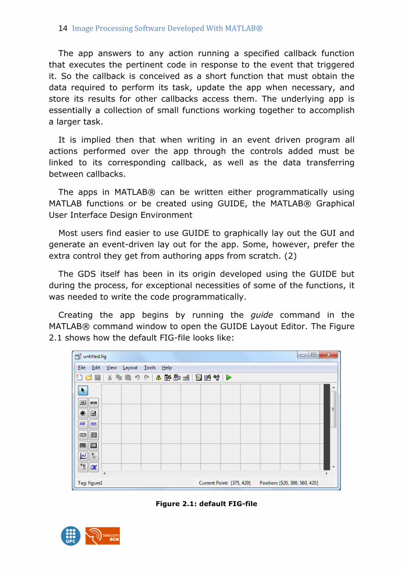
Creating the app begins by running the guide command in the
MATLAB® command window to open the GUIDE Layout Editor. The Figure
2.1 shows how the default FIG-file looks like:
Figure 2.1: default FIG-file
Image Processing Software Developed With MATLAB® 15
The GUIDE Layout Editor enables to define a GUI by clicking and
dragging GUI components into the layout area. The different elements
can be resized; buttons can be grouped and aligned, customized text
fields, sliders, axes, and add several other components. Other tools
accessible from the Layout Editor enable to:
Create menus and context menus
Create toolbars
Modify the appearance of components
Set tab order
View a hierarchical list of the component objects
Set GUI options
Once the UI has been defined the layout could be saved.
When a GUI is saved or run for the first time the GUIDE stores the GUI
in two files:
A FIG-file, with extension .fig, that contains a complete
description of the GUI layout and each UI component, such as push
buttons, axes, panels, menus, etc. The FIG-file is a non-modifiable
binary file, except by changing in the GUIDE the layout itself. FIG-
files are specializations of MAT-files.
A code file, with extension .m, that contains initialization
code and templates for some callbacks that control GUI behavior.
The user generally adds callbacks written for the UI components to
this file. As the callbacks are functions, the GUI code file can never
be a MATLAB® script.
The FIG-file and the code file must have the same name and are
usually placed in the same folder. Both files respectively correspond to
the tasks of laying out and programming the GUI. When the user designs
the layout of the GUI in the Layout Editor, their components and layout is
stored in the FIG-file. When the user programs the GUI, the code is
stored in the corresponding code file.(4)
16 Image Processing Software Developed With MATLAB®
2.2 Graphic Design Software - general
overview of the application
This section makes an introduction to the functional behavior of the
application beginning with a quick overview of the User Interface window
with a description of the different work areas.
Following there is a block diagram explaining the different apps
interaction. The GDS interacts with several simpler UIs developed to
configure the tool or preview the results before applying to the picture
and send the result back to the main application, the GDS.
2.2.1 Application window
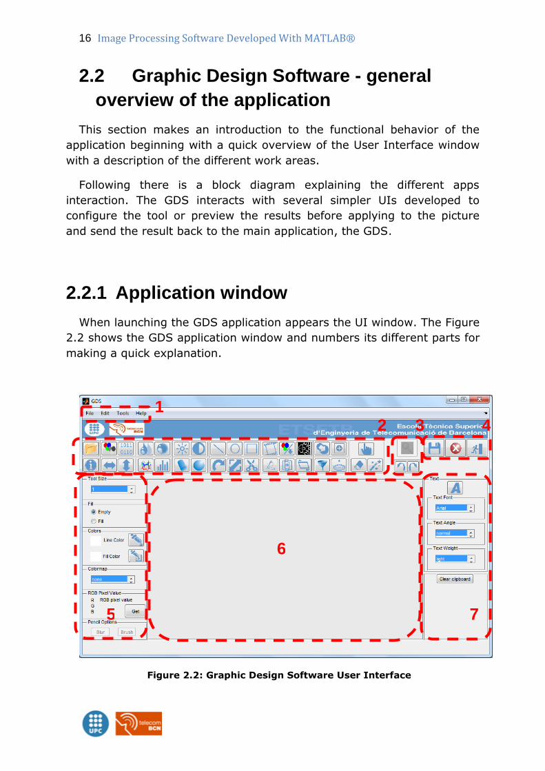
When launching the GDS application appears the UI window. The Figure
2.2 shows the GDS application window and numbers its different parts for
making a quick explanation.
Figure 2.2: Graphic Design Software User Interface
2 1
5 7
6
3 4
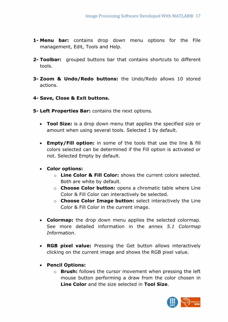
Image Processing Software Developed With MATLAB® 17
1- Menu bar: contains drop down menu options for the File
management, Edit, Tools and Help.
2- Toolbar: grouped buttons bar that contains shortcuts to different
tools.
3- Zoom & Undo/Redo buttons: the Undo/Redo allows 10 stored
actions.
4- Save, Close & Exit buttons.
5- Left Properties Bar: contains the next options.
Tool Size: is a drop down menu that applies the specified size or
amount when using several tools. Selected 1 by default.
Empty/Fill option: in some of the tools that use the line & fill
colors selected can be determined if the Fill option is activated or
not. Selected Empty by default.
Color options:
o Line Color & Fill Color: shows the current colors selected.
Both are white by default.
o Choose Color button: opens a chromatic table where Line
Color & Fill Color can interactively be selected.
o Choose Color Image button: select interactively the Line
Color & Fill Color in the current image.
Colormap: the drop down menu applies the selected colormap.
See more detailed information in the annex 5.1 Colormap
Information.
RGB pixel value: Pressing the Get button allows interactively
clicking on the current image and shows the RGB pixel value.
Pencil Options:
o Brush: follows the cursor movement when pressing the left
mouse button performing a draw from the color chosen in
Line Color and the size selected in Tool Size.
18 Image Processing Software Developed With MATLAB®
o Blur: follows the cursor movement when pressing the left
mouse button performing a blurring effect from the size
selected in Tool Size.
6- Workspace: area where the current image is placed and also for
performing the selected effects.
7- Right Properties Bar: include the Text and Clipboard options.
Text: pressing the Text button allows to enter a text on the
current image. Using the drop down menus to choose the font
type, weight and angle settings. The color chosen in Line Color
is the text color, the Fill Color is the background color, if the Fill
bullet is selected. The text size is selected in Tool Size.
Clipboard: the clipboard axes shows a saved image when:
o Using Copy option: the main picture in the Worskpace
axes is saved in the Clipboard axes. The saved undo/redo
actions are erased.
o Using Paste option: the main picture is restored to the
Workspace axes and the image to be pasted is saved in the
clipboard axes.
The Clear Clipboard button erases any image saved in the
clipboard axes.
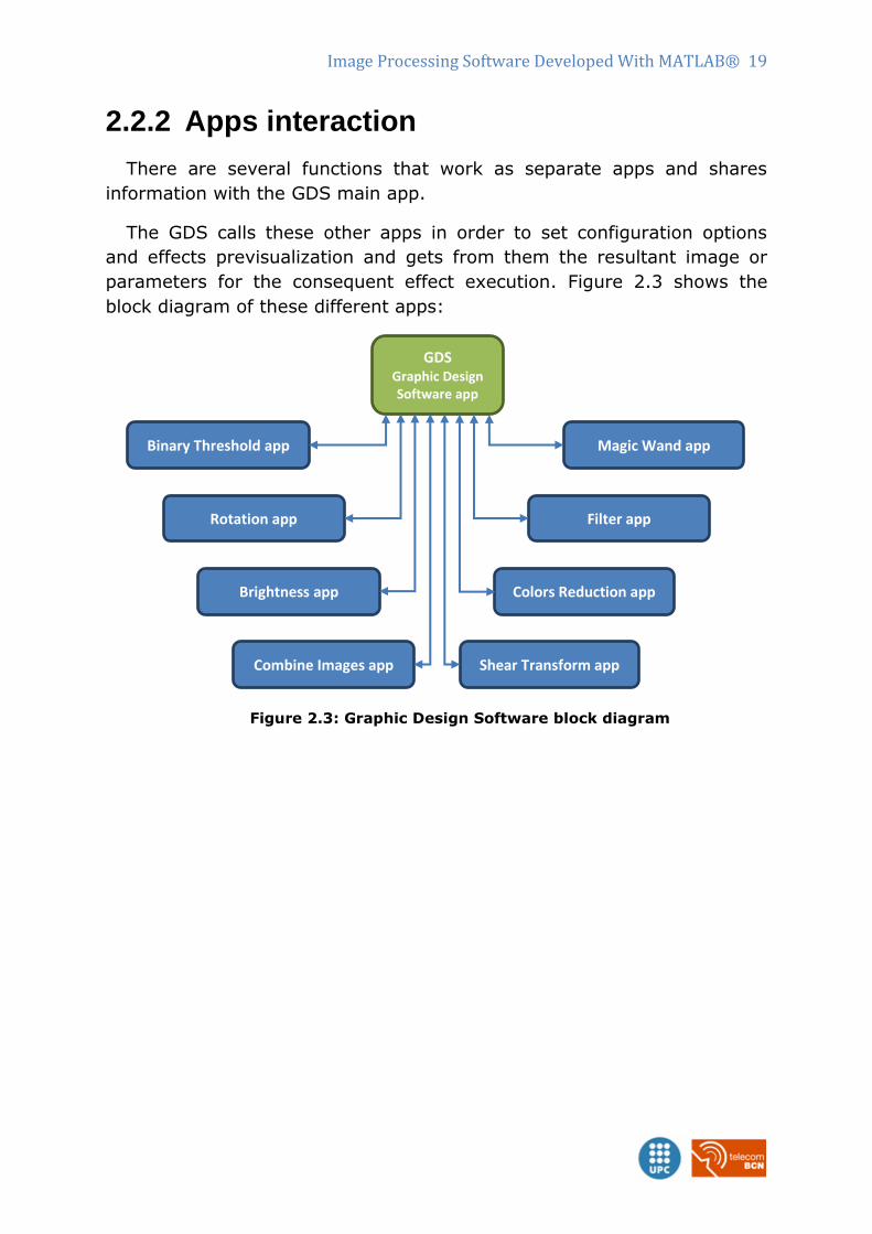
Image Processing Software Developed With MATLAB® 19
2.2.2 Apps interaction
There are several functions that work as separate apps and shares
information with the GDS main app.
The GDS calls these other apps in order to set configuration options
and effects previsualization and gets from them the resultant image or
parameters for the consequent effect execution. Figure 2.3 shows the
block diagram of these different apps:
Figure 2.3: Graphic Design Software block diagram
GDS Graphic Design Software app
Binary Threshold app
Rotation app
Brightness app
Combine Images app Shear Transform app
Colors Reduction app
Filter app
Magic Wand app
20 Image Processing Software Developed With MATLAB®
2.3 Image Processing Tools
This section presents a complete description of all the tools developed
for the GDS application.
The tool descriptions are grouped according to the GDS GUI parts from
section 2.2.1 Application window. It is shown the icon that represents the
tool, the MATLAB® functions used for the implementation and extracts
from the code to explain the programming.
It is described in detail the specific behavior or step sequences for
running the more complex tools.
The code extracts in most cases are a simplified version of the code for
a better quick comprehension, but the complete code of the GDS
application is in annex 5.7 GDS.m code.
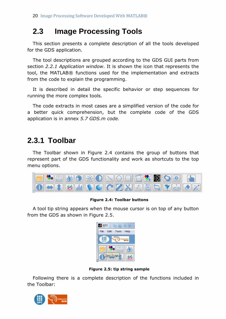
2.3.1 Toolbar
The Toolbar shown in Figure 2.4 contains the group of buttons that
represent part of the GDS functionality and work as shortcuts to the top
menu options.
Figure 2.4: Toolbar buttons
A tool tip string appears when the mouse cursor is on top of any button
from the GDS as shown in Figure 2.5.
Figure 2.5: tip string sample
Following there is a complete description of the functions included in
the Toolbar:
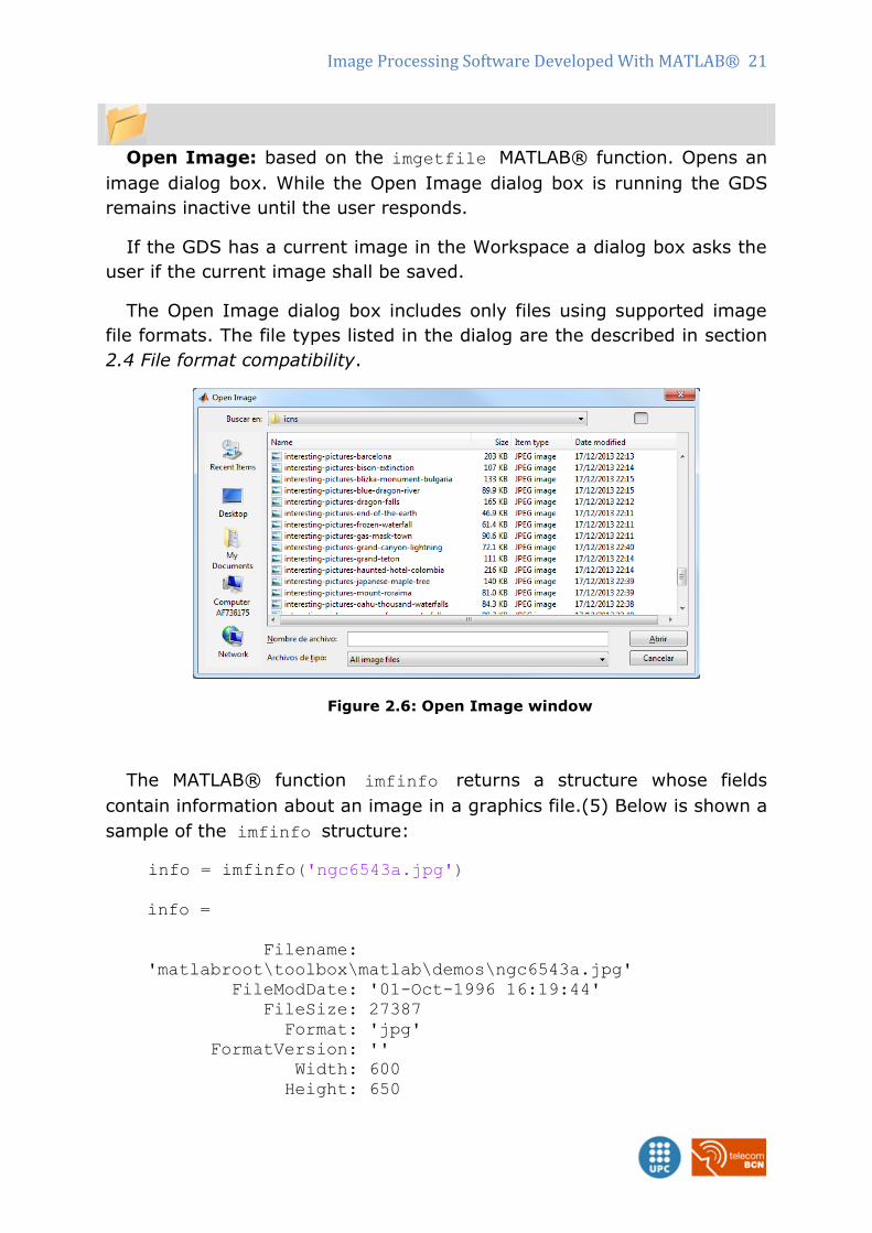
Image Processing Software Developed With MATLAB® 21
Open Image: based on the imgetfile MATLAB® function. Opens an
image dialog box. While the Open Image dialog box is running the GDS
remains inactive until the user responds.
If the GDS has a current image in the Workspace a dialog box asks the
user if the current image shall be saved.
The Open Image dialog box includes only files using supported image
file formats. The file types listed in the dialog are the described in section
2.4 File format compatibility.
Figure 2.6: Open Image window
The MATLAB® function imfinfo returns a structure whose fields
contain information about an image in a graphics file.(5) Below is shown a
sample of the imfinfo structure:
info = imfinfo('ngc6543a.jpg')
info =
Filename:
'matlabroot\toolbox\matlab\demos\ngc6543a.jpg'
FileModDate: '01-Oct-1996 16:19:44'
FileSize: 27387
Format: 'jpg'
FormatVersion: ''
Width: 600
Height: 650
22 Image Processing Software Developed With MATLAB®
BitDepth: 24
ColorType: 'truecolor'
FormatSignature: ''
NumberOfSamples: 3
CodingMethod: 'Huffman'
CodingProcess: 'Sequential'
Comment: {'CREATOR: XV Version 3.00b Rev:
6/15/94 Quality = 75, Smoothing = 0'}
The BitDepth means the bits per sampled pixel images and it is needed
in other tools as Brightness or Binary Threshold.
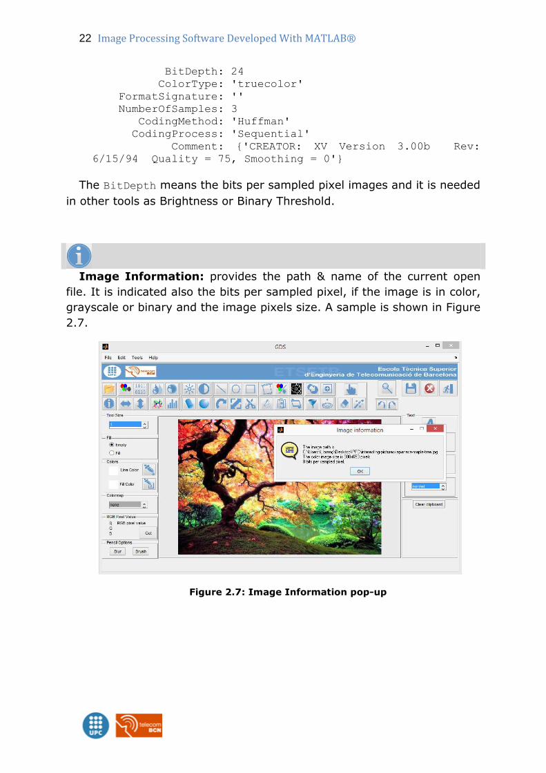
Image Information: provides the path & name of the current open
file. It is indicated also the bits per sampled pixel, if the image is in color,
grayscale or binary and the image pixels size. A sample is shown in Figure
2.7.
Figure 2.7: Image Information pop-up
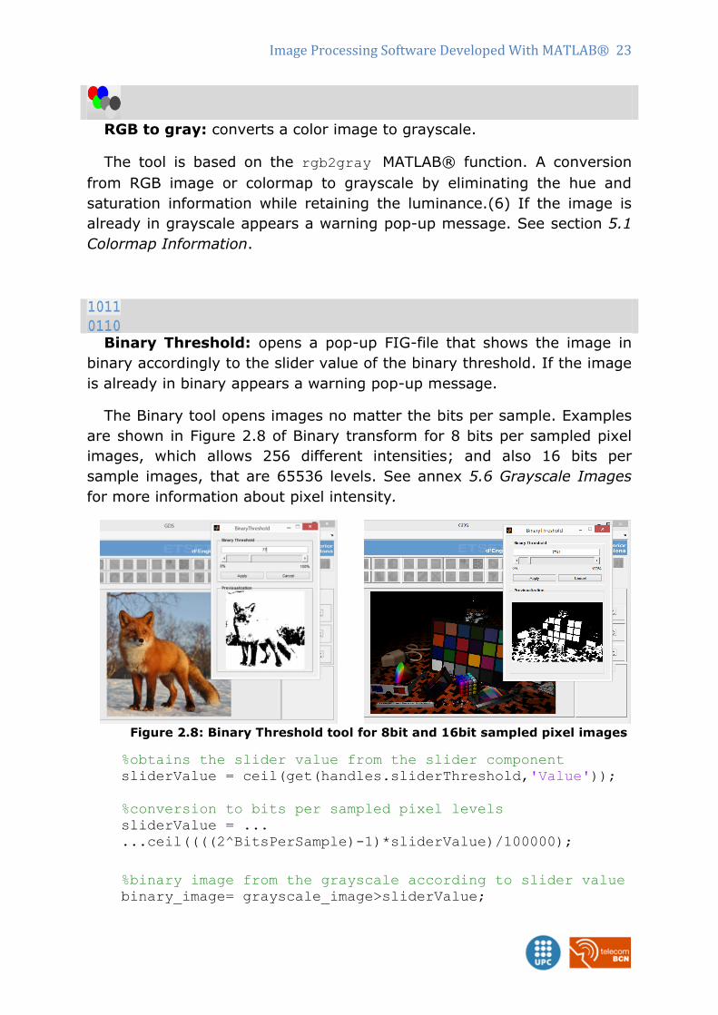
Image Processing Software Developed With MATLAB® 23
RGB to gray: converts a color image to grayscale.
The tool is based on the rgb2gray MATLAB® function. A conversion
from RGB image or colormap to grayscale by eliminating the hue and
saturation information while retaining the luminance.(6) If the image is
already in grayscale appears a warning pop-up message. See section 5.1
Colormap Information.
Binary Threshold: opens a pop-up FIG-file that shows the image in
binary accordingly to the slider value of the binary threshold. If the image
is already in binary appears a warning pop-up message.
The Binary tool opens images no matter the bits per sample. Examples
are shown in Figure 2.8 of Binary transform for 8 bits per sampled pixel
images, which allows 256 different intensities; and also 16 bits per
sample images, that are 65536 levels. See annex 5.6 Grayscale Images
for more information about pixel intensity.
Figure 2.8: Binary Threshold tool for 8bit and 16bit sampled pixel images
%obtains the slider value from the slider component sliderValue = ceil(get(handles.sliderThreshold,'Value'));
%conversion to bits per sampled pixel levels
sliderValue = ...
...ceil((((2^BitsPerSample)-1)*sliderValue)/100000);
%binary image from the grayscale according to slider value
binary_image= grayscale_image>sliderValue;
24 Image Processing Software Developed With MATLAB®
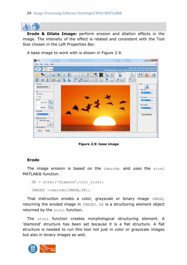
Erode & Dilate Image: perform erosion and dilation effects in the
image. The intensity of the effect is related and consistent with the Tool
Size chosen in the Left Properties Bar.
A base image to work with is shown in Figure 2.9.
Figure 2.9: base image
Erode
The image erosion is based on the imerode and uses the strel
MATLAB® function.
SE = strel('diamond',tool_size);
IMAGE2 =imerode(IMAGE,SE);
That instruction erodes a color, grayscale or binary image IMAGE,
returning the eroded image in IMAGE2. SE is a structuring element object
returned by the strel function.
The strel function creates morphological structuring element. A
„diamond‟ structure has been set because it is a flat structure. A flat
structure is needed to run this tool not just in color or grayscale images
but also in binary images as well.
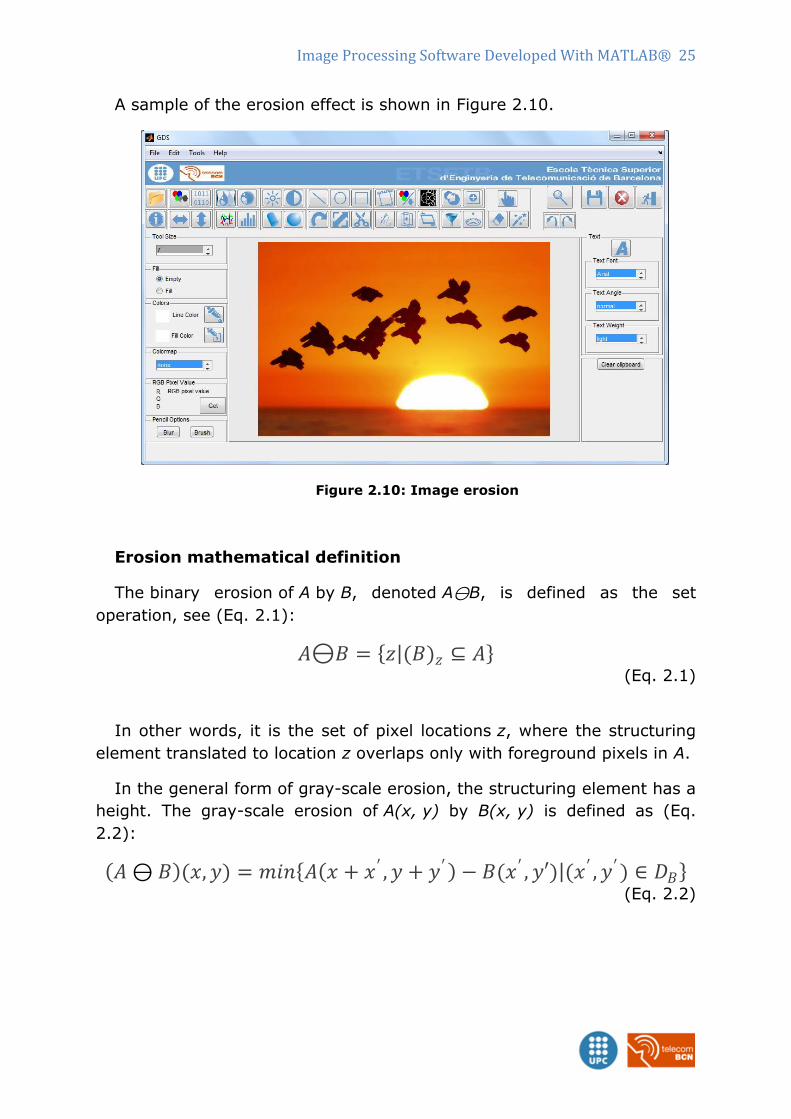
Image Processing Software Developed With MATLAB® 25
A sample of the erosion effect is shown in Figure 2.10.
Figure 2.10: Image erosion
Erosion mathematical definition
The binary erosion of A by B, denoted A⊖B, is defined as the set
operation, see (Eq. 2.1):
𝐴⊖𝐵 = 𝑧 (𝐵)𝑧 ⊆ 𝐴 (Eq. 2.1)
In other words, it is the set of pixel locations z, where the structuring
element translated to location z overlaps only with foreground pixels in A.
In the general form of gray-scale erosion, the structuring element has a
height. The gray-scale erosion of A(x, y) by B(x, y) is defined as (Eq.
2.2):
𝐴 ⊖ 𝐵 (𝑥, 𝑦) = 𝑚𝑖𝑛 𝐴 𝑥 + 𝑥′ , 𝑦 + 𝑦′ − 𝐵(𝑥′ , 𝑦′) (𝑥 ′ , 𝑦′) ∈ 𝐷𝐵 (Eq. 2.2)
26 Image Processing Software Developed With MATLAB®
Where DB is the domain of the structuring element B and A(x,y) is
assumed to be +∞ outside the domain of the image. To create a
structuring element with nonzero height values, use the
syntax strel(nhood,height), where height gives the height values
and nhood corresponds to the structuring element domain, DB.
Most commonly, gray-scale erosion is performed with a flat structuring
element (B(x,y)=0). Gray-scale erosion using such a structuring element
is equivalent to a local-minimum operator, see (Eq. 2.3):
𝐴 ⊖ 𝐵 (𝑥, 𝑦) = 𝑚𝑖𝑛 𝐴 𝑥 + 𝑥′ , 𝑦 + 𝑦′ (𝑥′ , 𝑦′) ∈ 𝐷𝐵
(Eq. 2.3)
(7)
Dilate
The image dilation is based on the imdilate and use the strel
MATLAB® function.
SE = strel('diamond',tool_size);
IMAGE2 = imdilate(IMAGE,SE);
That instruction dilates a color, grayscale or binary image IMAGE,
returning the dilated image in IMAGE2. SE is a structuring element object
returned by the strel function.
The strel function creates morphological structuring element. A
„diamond‟ structure has been set because it is a flat structure. A flat
structure is needed to run this tool not just in color or grayscale images
but also in binary images as well.
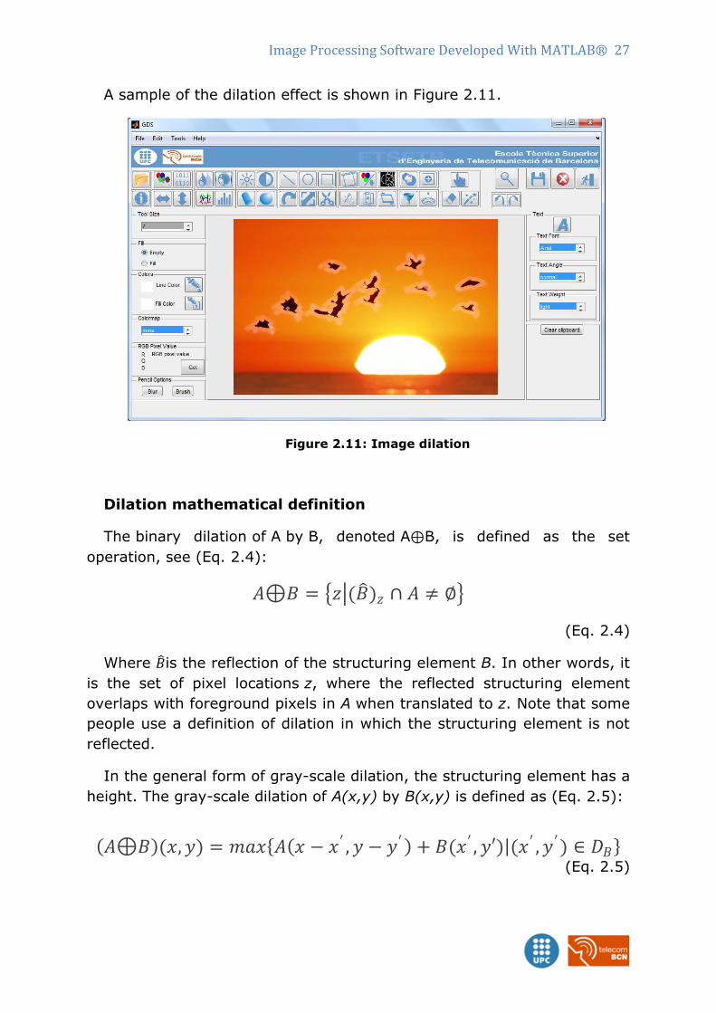
Image Processing Software Developed With MATLAB® 27
A sample of the dilation effect is shown in Figure 2.11.
Figure 2.11: Image dilation
Dilation mathematical definition
The binary dilation of A by B, denoted A⊕B, is defined as the set
operation, see (Eq. 2.4):
𝐴⊕𝐵 = 𝑧 (𝐵 )𝑧 ∩ 𝐴 ≠ ∅
(Eq. 2.4)
Where 𝐵 is the reflection of the structuring element B. In other words, it
is the set of pixel locations z, where the reflected structuring element
overlaps with foreground pixels in A when translated to z. Note that some
people use a definition of dilation in which the structuring element is not
reflected.
In the general form of gray-scale dilation, the structuring element has a
height. The gray-scale dilation of A(x,y) by B(x,y) is defined as (Eq. 2.5):
𝐴⊕𝐵 (𝑥, 𝑦) = 𝑚𝑎𝑥 𝐴 𝑥 − 𝑥′ , 𝑦 − 𝑦′ + 𝐵(𝑥′ , 𝑦′) (𝑥′ , 𝑦′) ∈ 𝐷𝐵 (Eq. 2.5)
28 Image Processing Software Developed With MATLAB®
Where DB is the domain of the structuring element B and A(x,y) is
assumed to be −∞ outside the domain of the image. To create a
structuring element with nonzero height values, use the
syntax strel(nhood,height), where height gives the height values
and nhood corresponds to the structuring element domain, DB.
Most commonly, gray-scale dilation is performed with a flat structuring
element (B(x,y)=0). Gray-scale dilation using such a structuring element
is equivalent to a local-maximum operator, see (Eq. 2.6):
𝐴⊕𝐵 (𝑥, 𝑦) = 𝑚𝑎𝑥 𝐴(𝑥 − 𝑥′, 𝑦 − 𝑦′) (𝑥′ , 𝑦′) ∈ 𝐷𝐵 (Eq. 2.6)
(8)
Horizontal & Vertical Flip: execute a flip in the horizontal or vertical
axe of the image.
The flipping is based on the flipdim MATLAB® function; it flips an
array along the specified dimension:
IMAGE2 = flipdim(IMAGE,dim)
When the value of dim is 1, the array is flipped row-wise down. When
dim is 2, the array is flipped column-wise left to right.(9)
Cylinder & Sphere Deformation: create a new window with the
current image placed on to a cylinder or a sphere shape, a 3D rotation
can be performed to choose the position desired.
Both effects are based on cylinder, sphere respectively and warp
MATLAB® functions.
Cylinder Deformation
[X,Y,Z] = cylinder(R,N);
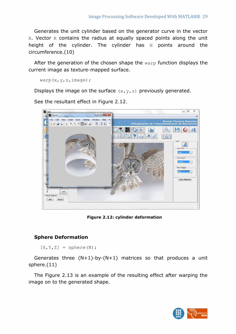
Image Processing Software Developed With MATLAB® 29
Generates the unit cylinder based on the generator curve in the vector
R. Vector R contains the radius at equally spaced points along the unit
height of the cylinder. The cylinder has N points around the
circumference.(10)
After the generation of the chosen shape the warp function displays the
current image as texture-mapped surface.
warp(x,y,z,image);
Displays the image on the surface (x,y,z) previously generated.
See the resultant effect in Figure 2.12.
Figure 2.12: cylinder deformation
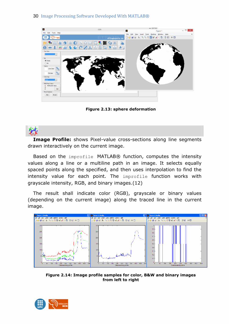
Sphere Deformation
[X,Y,Z] = sphere(N);
Generates three (N+1)-by-(N+1) matrices so that produces a unit
sphere.(11)
The Figure 2.13 is an example of the resulting effect after warping the
image on to the generated shape.
30 Image Processing Software Developed With MATLAB®
Figure 2.13: sphere deformation
Image Profile: shows Pixel-value cross-sections along line segments
drawn interactively on the current image.
Based on the improfile MATLAB® function, computes the intensity
values along a line or a multiline path in an image. It selects equally
spaced points along the specified, and then uses interpolation to find the
intensity value for each point. The improfile function works with
grayscale intensity, RGB, and binary images.(12)
The result shall indicate color (RGB), grayscale or binary values
(depending on the current image) along the traced line in the current
image.
Figure 2.14: Image profile samples for color, B&W and binary images
from left to right
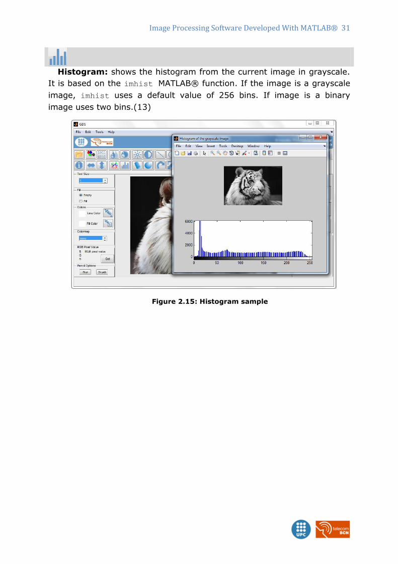
Image Processing Software Developed With MATLAB® 31
Histogram: shows the histogram from the current image in grayscale.
It is based on the imhist MATLAB® function. If the image is a grayscale
image, imhist uses a default value of 256 bins. If image is a binary
image uses two bins.(13)
Figure 2.15: Histogram sample
32 Image Processing Software Developed With MATLAB®
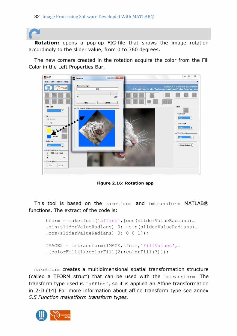
Rotation: opens a pop-up FIG-file that shows the image rotation
accordingly to the slider value, from 0 to 360 degrees.
The new corners created in the rotation acquire the color from the Fill
Color in the Left Properties Bar.
Figure 2.16: Rotation app
This tool is based on the maketform and imtransform MATLAB®
functions. The extract of the code is:
tform = maketform('affine',[cos(sliderValueRadians)…
…sin(sliderValueRadians) 0; -sin(sliderValueRadians)…
…cos(sliderValueRadians) 0; 0 0 1]);
IMAGE2 = imtransform(IMAGE,tform,'FillValues',…
…[colorFill(1);colorFill(2);colorFill(3)]);
maketform creates a multidimensional spatial transformation structure
(called a TFORM struct) that can be used with the imtransform. The
transform type used is 'affine', so it is applied an Affine transformation
in 2-D.(14) For more information about affine transform type see annex
5.5 Function maketform transform types.
Image Processing Software Developed With MATLAB® 33
imtransform applies 2-D spatial transformation to image. The
parameter 'FillValues' consist in an optional comma-separated pairs of
Name/Value arguments. It is an array containing one or several fill
values. The imtransform function uses fill values for output pixels when
the corresponding transformed location in the input image is completely
outside the input image boundaries, and uses the Fill Color selected in the
Left Properties Bar. If IMAGE was 2-D,'FillValues' requires a scalar.
However, if IMAGE's dimension is greater than two, then could be specified
'FillValues' as an array whose size satisfies the following constraint:
size(fill_values,k) must equal either size(A,k+2) or 1.(15)
Resize: based on the imresize MATLAB® function to resize images.
IMAGE2 = imresize(IMAGE, SCALE);
Returns IMAGE2 that is SCALE times the size of IMAGE, which is a
grayscale, RGB, or binary image.(16)
For computing reasons it is limited to values between 1 and 10 to
enlarge and between 0 and 1 to reduce.
Crop: based on the imcrop MATLAB® function to crop images. Creates
an interactive image cropping tool. It is a moveable, resizable rectangle
that is interactively placed and manipulated using the mouse. After
positioning the tool, the user crops the target image by either double
clicking on the tool or choosing 'Crop Image' from the tool's context
menu. The cropped image is returned.
The cropping tool can be deleted by pressing backspace, escape, or
delete, or via the 'Cancel' option from the context menu. If the tool is
deleted, all return values are set to empty.(17)
34 Image Processing Software Developed With MATLAB®
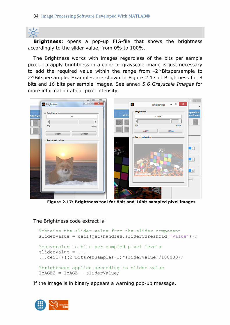
Brightness: opens a pop-up FIG-file that shows the brightness
accordingly to the slider value, from 0% to 100%.
The Brightness works with images regardless of the bits per sample
pixel. To apply brightness in a color or grayscale image is just necessary
to add the required value within the range from -2^Bitspersample to
2^Bitspersample. Examples are shown in Figure 2.17 of Brightness for 8
bits and 16 bits per sample images. See annex 5.6 Grayscale Images for
more information about pixel intensity.
Figure 2.17: Brightness tool for 8bit and 16bit sampled pixel images
The Brightness code extract is:
%obtains the slider value from the slider component sliderValue = ceil(get(handles.sliderThreshold,'Value'));
%conversion to bits per sampled pixel levels
sliderValue = ...
...ceil((((2^BitsPerSample)-1)*sliderValue)/100000);
%brightness applied according to slider value
IMAGE2 = IMAGE + sliderValue;
If the image is in binary appears a warning pop-up message.
Image Processing Software Developed With MATLAB® 35
Auto Contrast: based on the max(x) & min(x) MATLAB® functions.
Applying these in matrices max(X) & max(X) returns a row vector
containing the maximum or minimum element from each column. Both
functions are used to find the higher & lower pixel value in the current
picture. For RGB images this procedure is applied in the 3 matrices.
To perform the auto contrast the matrix that is our image is scaled
within zero and 2^Bits per Sample. To do so the original picture is
subtracted the minimum value and multiplied by the 2^Bits per Sample
divided the bit value range to produce the auto contrast enhancement.
mx = max(max(picture)) ;
mn = min(min(picture));
IMAGE_MN = IMAGE-mn;
RATIO=2^(BitsPerSample)/(mx-mn);
Auto_Contrast_IMAGE = IMAGE_MN *RATIO;
In case the image has already a proper contrast a pop-up warning is
shown.
36 Image Processing Software Developed With MATLAB®
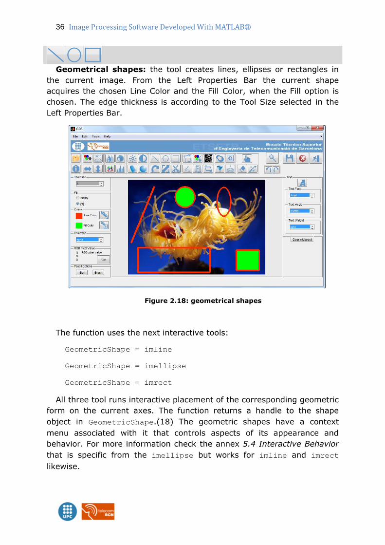
Geometrical shapes: the tool creates lines, ellipses or rectangles in
the current image. From the Left Properties Bar the current shape
acquires the chosen Line Color and the Fill Color, when the Fill option is
chosen. The edge thickness is according to the Tool Size selected in the
Left Properties Bar.
Figure 2.18: geometrical shapes
The function uses the next interactive tools:
GeometricShape = imline
GeometricShape = imellipse
GeometricShape = imrect
All three tool runs interactive placement of the corresponding geometric
form on the current axes. The function returns a handle to the shape
object in GeometricShape.(18) The geometric shapes have a context
menu associated with it that controls aspects of its appearance and
behavior. For more information check the annex 5.4 Interactive Behavior
that is specific from the imellipse but works for imline and imrect
likewise.
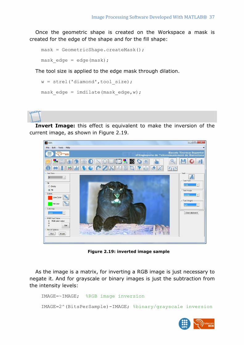
Image Processing Software Developed With MATLAB® 37
Once the geometric shape is created on the Workspace a mask is
created for the edge of the shape and for the fill shape:
mask = GeometricShape.createMask();
mask_edge = edge(mask);
The tool size is applied to the edge mask through dilation.
w = strel('diamond',tool_size);
mask_edge = imdilate(mask_edge,w);
Invert Image: this effect is equivalent to make the inversion of the
current image, as shown in Figure 2.19.
Figure 2.19: inverted image sample
As the image is a matrix, for inverting a RGB image is just necessary to
negate it. And for grayscale or binary images is just the subtraction from
the intensity levels:
IMAGE=~IMAGE; %RGB image inversion
IMAGE=2^(BitsPerSample)-IMAGE; %binary/grayscale inversion
38 Image Processing Software Developed With MATLAB®
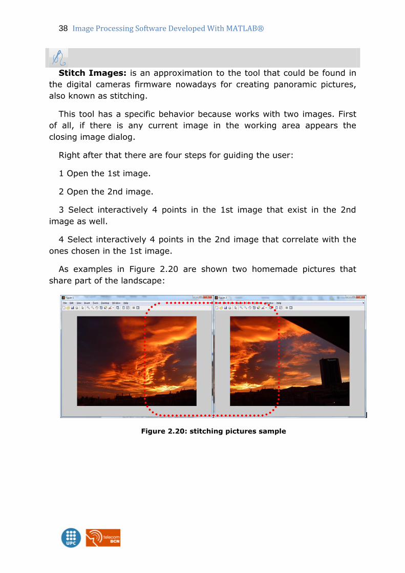
Stitch Images: is an approximation to the tool that could be found in
the digital cameras firmware nowadays for creating panoramic pictures,
also known as stitching.
This tool has a specific behavior because works with two images. First
of all, if there is any current image in the working area appears the
closing image dialog.
Right after that there are four steps for guiding the user:
1 Open the 1st image.
2 Open the 2nd image.
3 Select interactively 4 points in the 1st image that exist in the 2nd
image as well.
4 Select interactively 4 points in the 2nd image that correlate with the
ones chosen in the 1st image.
As examples in Figure 2.20 are shown two homemade pictures that
share part of the landscape:
Figure 2.20: stitching pictures sample
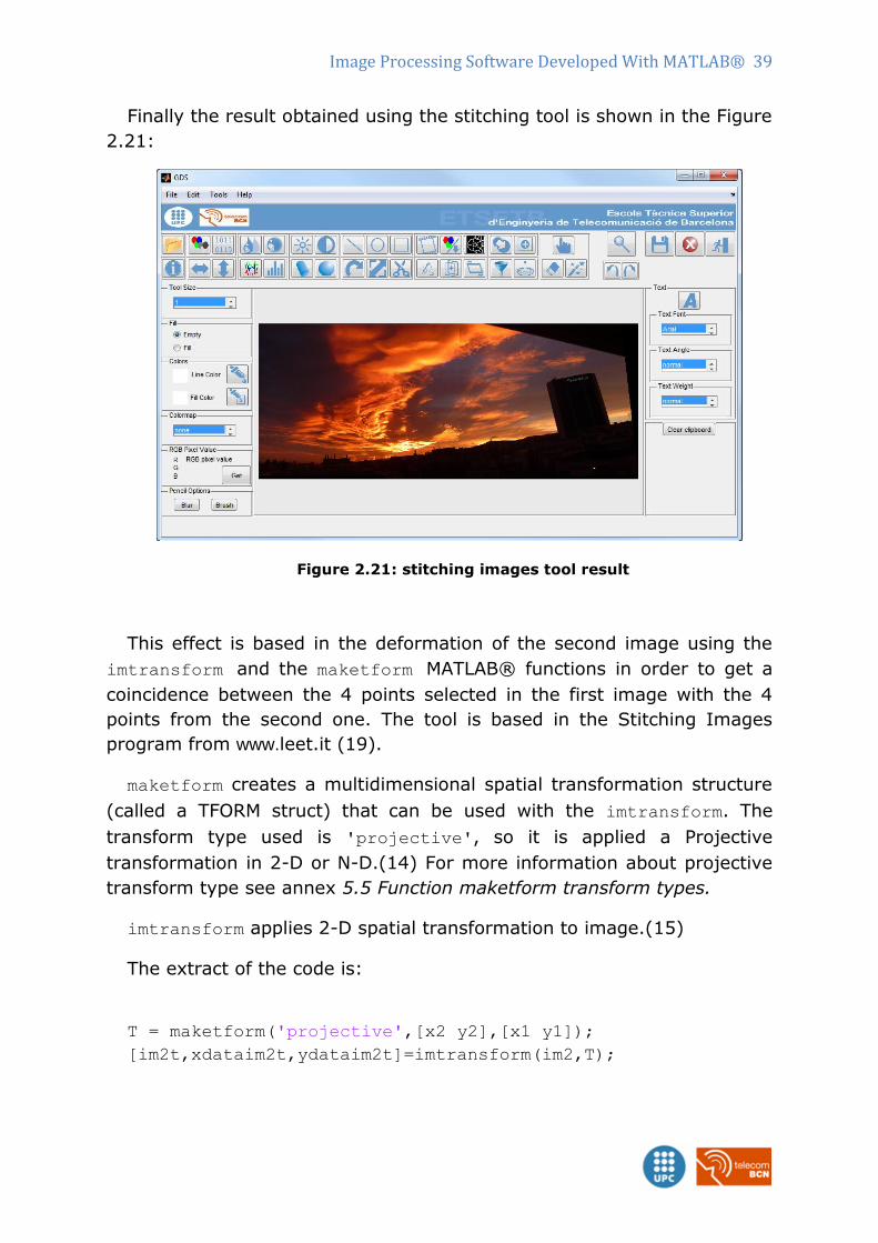
Image Processing Software Developed With MATLAB® 39
Finally the result obtained using the stitching tool is shown in the Figure
2.21:
Figure 2.21: stitching images tool result
This effect is based in the deformation of the second image using the
imtransform and the maketform MATLAB® functions in order to get a
coincidence between the 4 points selected in the first image with the 4
points from the second one. The tool is based in the Stitching Images
program from www.leet.it (19).
maketform creates a multidimensional spatial transformation structure
(called a TFORM struct) that can be used with the imtransform. The
transform type used is 'projective', so it is applied a Projective
transformation in 2-D or N-D.(14) For more information about projective
transform type see annex 5.5 Function maketform transform types.
imtransform applies 2-D spatial transformation to image.(15)
The extract of the code is:
T = maketform('projective',[x2 y2],[x1 y1]);
[im2t,xdataim2t,ydataim2t]=imtransform(im2,T);
40 Image Processing Software Developed With MATLAB®
%now xdataim2t & ydataim2t store the bounds...
... of the transformed im2
xdataout = [min(1,xdataim2t(1))…
…max(size(im1,2),xdataim2t(2))];
ydataout = [min(1,ydataim2t(1))…
…max(size(im1,1),ydataim2t(2))];
%transform both images with the computed xdata and ydata
im2t = imtransform(im2,T,'XData',xdataout,'YData',ydataout);
im1t = imtransform(im1,maketform('affine',eye(3)),'XData',…
…xdataout,'YData',ydataout);
picture=max(im1t,im2t);
Image Combination: performs a combination of two images changing
inversely proportional the opacity in both images.
This tool has a specific behavior because works with two images. First
of all, if there is any current image in the working area appears the
closing image dialog.
Right after that there are three steps for guiding the user:
1 Open the background image.
2 Open the foreground image.
3 Then a pop-up FIG-file is shown, where both images are combined
accordingly to the slider value for the opacity, from 0 to 1.
The image resulting of the combination preserves the size, path and
name of the background image.
If both images do not have the same dimensions because one image is
RGB and the other is binary the tool modifies the binary creating a 3
dimensional matrix to match with an RGB image. The process is
transparent to the user.
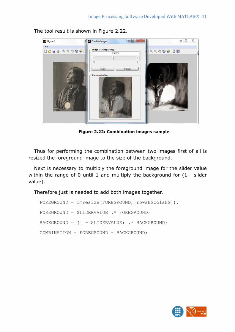
Image Processing Software Developed With MATLAB® 41
The tool result is shown in Figure 2.22.
Figure 2.22: Combination images sample
Thus for performing the combination between two images first of all is
resized the foreground image to the size of the background.
Next is necessary to multiply the foreground image for the slider value
within the range of 0 until 1 and multiply the background for (1 - slider
value).
Therefore just is needed to add both images together.
FOREGROUND = imresize(FOREGROUND,[rowsBGcolsBG]);
FOREGROUND = SLIDERVALUE .* FOREGROUND;
BACKGROUND = (1 - SLIDERVALUE) .* BACKGROUND;
COMBINATION = FOREGROUND + BACKGROUND;
42 Image Processing Software Developed With MATLAB®
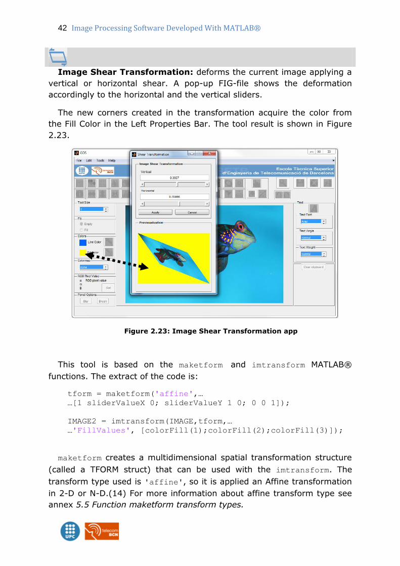
Image Shear Transformation: deforms the current image applying a
vertical or horizontal shear. A pop-up FIG-file shows the deformation
accordingly to the horizontal and the vertical sliders.
The new corners created in the transformation acquire the color from
the Fill Color in the Left Properties Bar. The tool result is shown in Figure
2.23.
Figure 2.23: Image Shear Transformation app
This tool is based on the maketform and imtransform MATLAB®
functions. The extract of the code is:
tform = maketform('affine',…
…[1 sliderValueX 0; sliderValueY 1 0; 0 0 1]);
IMAGE2 = imtransform(IMAGE,tform,…
…'FillValues', [colorFill(1);colorFill(2);colorFill(3)]);
maketform creates a multidimensional spatial transformation structure
(called a TFORM struct) that can be used with the imtransform. The
transform type used is 'affine', so it is applied an Affine transformation
in 2-D or N-D.(14) For more information about affine transform type see
annex 5.5 Function maketform transform types.
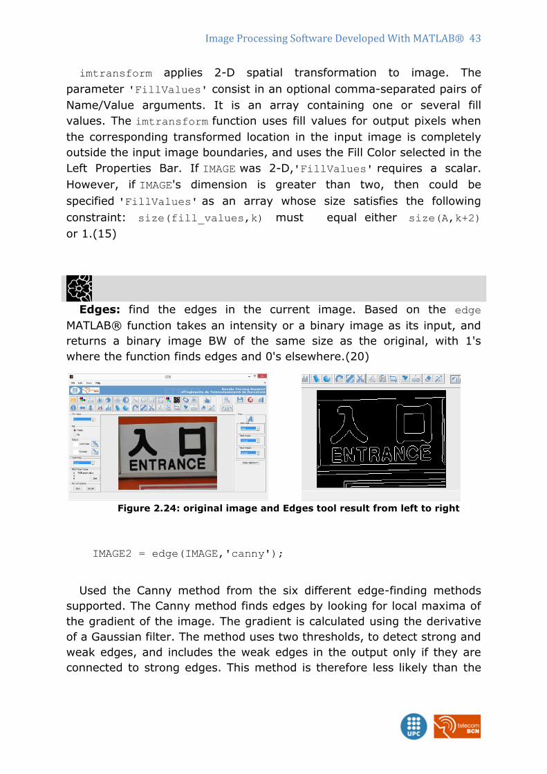
Image Processing Software Developed With MATLAB® 43
imtransform applies 2-D spatial transformation to image. The
parameter 'FillValues' consist in an optional comma-separated pairs of
Name/Value arguments. It is an array containing one or several fill
values. The imtransform function uses fill values for output pixels when
the corresponding transformed location in the input image is completely
outside the input image boundaries, and uses the Fill Color selected in the
Left Properties Bar. If IMAGE was 2-D,'FillValues' requires a scalar.
However, if IMAGE's dimension is greater than two, then could be
specified 'FillValues' as an array whose size satisfies the following
constraint: size(fill_values,k) must equal either size(A,k+2)
or 1.(15)
Edges: find the edges in the current image. Based on the edge
MATLAB® function takes an intensity or a binary image as its input, and
returns a binary image BW of the same size as the original, with 1's
where the function finds edges and 0's elsewhere.(20)
Figure 2.24: original image and Edges tool result from left to right
IMAGE2 = edge(IMAGE,'canny');
Used the Canny method from the six different edge-finding methods
supported. The Canny method finds edges by looking for local maxima of
the gradient of the image. The gradient is calculated using the derivative
of a Gaussian filter. The method uses two thresholds, to detect strong and
weak edges, and includes the weak edges in the output only if they are
connected to strong edges. This method is therefore less likely than the
44 Image Processing Software Developed With MATLAB®
others to be "fooled" by noise, and more likely to detect true weak
edges.(21)
If the image is already in binary appears a warning pop-up message.
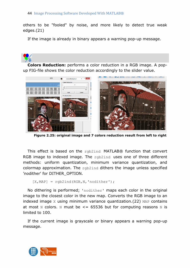
Colors Reduction: performs a color reduction in a RGB image. A pop-
up FIG-file shows the color reduction accordingly to the slider value.
Figure 2.25: original image and 7 colors reduction result from left to right
This effect is based on the rgb2ind MATLAB® function that convert
RGB image to indexed image. The rgb2ind uses one of three different
methods: uniform quantization, minimum variance quantization, and
colormap approximation. The rgb2ind dithers the image unless specified
'nodither' for DITHER_OPTION.
[X,MAP] = rgb2ind(RGB,N,'nodither');
No dithering is performed; 'nodither' maps each color in the original
image to the closest color in the new map. Converts the RGB image to an
indexed image X using minimum variance quantization.(22) MAP contains
at most N colors. N must be <= 65536 but for computing reasons N is
limited to 100.
If the current image is grayscale or binary appears a warning pop-up
message.
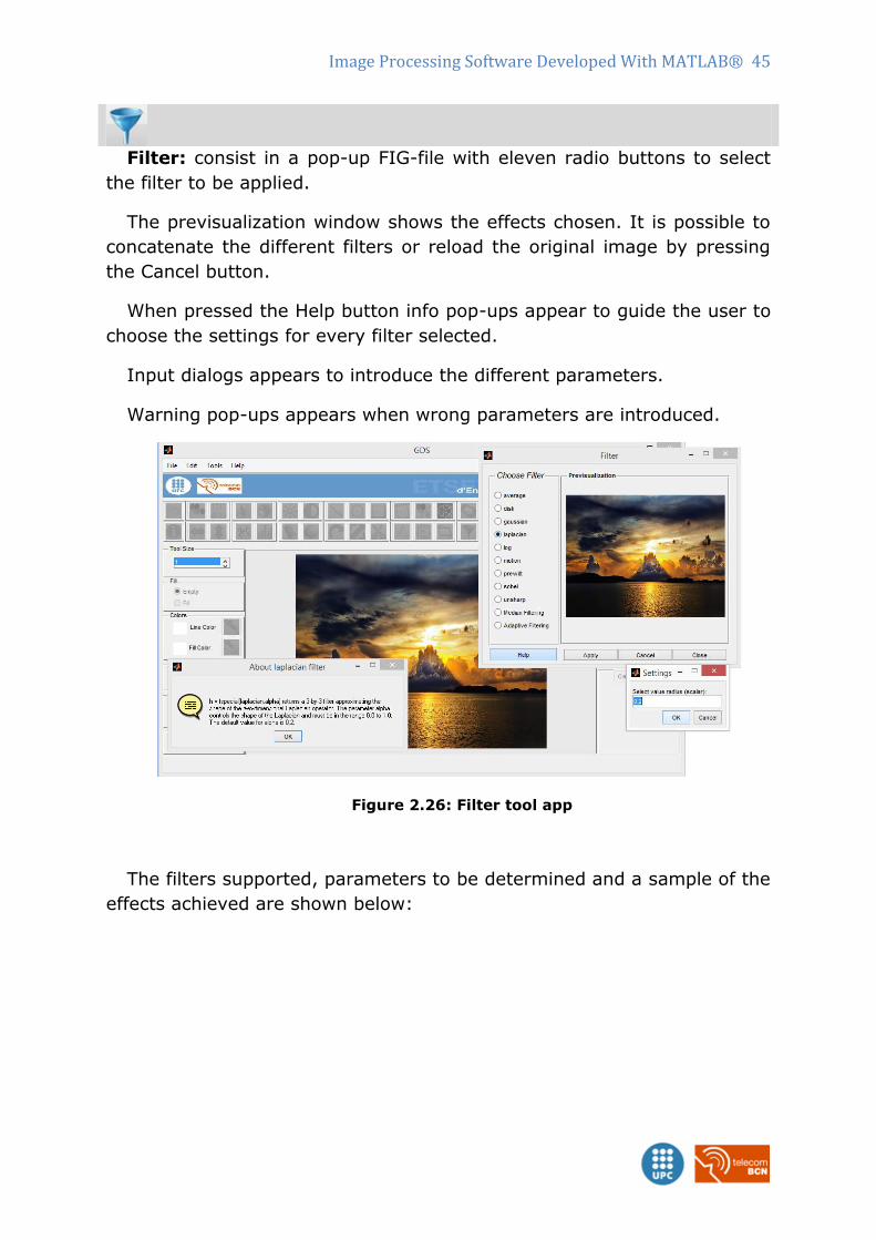
Image Processing Software Developed With MATLAB® 45
Filter: consist in a pop-up FIG-file with eleven radio buttons to select
the filter to be applied.
The previsualization window shows the effects chosen. It is possible to
concatenate the different filters or reload the original image by pressing
the Cancel button.
When pressed the Help button info pop-ups appear to guide the user to
choose the settings for every filter selected.
Input dialogs appears to introduce the different parameters.
Warning pop-ups appears when wrong parameters are introduced.
Figure 2.26: Filter tool app
The filters supported, parameters to be determined and a sample of the
effects achieved are shown below:
46 Image Processing Software Developed With MATLAB®
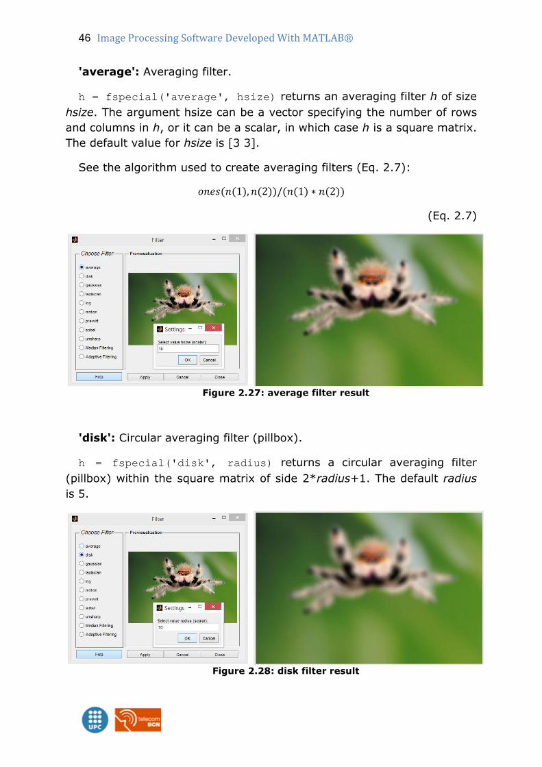
'average': Averaging filter.
h = fspecial('average', hsize) returns an averaging filter h of size
hsize. The argument hsize can be a vector specifying the number of rows
and columns in h, or it can be a scalar, in which case h is a square matrix.
The default value for hsize is [3 3].
See the algorithm used to create averaging filters (Eq. 2.7):
𝑜𝑛𝑒𝑠(𝑛(1), 𝑛(2))/(𝑛(1) ∗ 𝑛(2))
(Eq. 2.7)
Figure 2.27: average filter result
'disk': Circular averaging filter (pillbox).
h = fspecial('disk', radius) returns a circular averaging filter
(pillbox) within the square matrix of side 2*radius+1. The default radius
is 5.
Figure 2.28: disk filter result
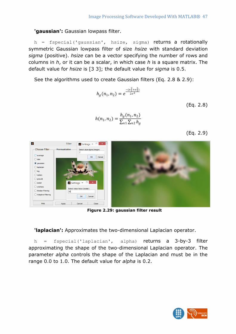
Image Processing Software Developed With MATLAB® 47
'gaussian': Gaussian lowpass filter.
h = fspecial('gaussian', hsize, sigma) returns a rotationally
symmetric Gaussian lowpass filter of size hsize with standard deviation
sigma (positive). hsize can be a vector specifying the number of rows and
columns in h, or it can be a scalar, in which case h is a square matrix. The
default value for hsize is [3 3]; the default value for sigma is 0.5.
See the algorithms used to create Gaussian filters (Eq. 2.8 & 2.9):
ℎ𝑔(𝑛1, 𝑛2) = 𝑒−(𝑛1
2+𝑛22)
2𝜎2
(Eq. 2.8)
ℎ(𝑛1, 𝑛2) =ℎ𝑔(𝑛1, 𝑛2)
ℎ𝑔𝑛2𝑛1
(Eq. 2.9)
Figure 2.29: gaussian filter result
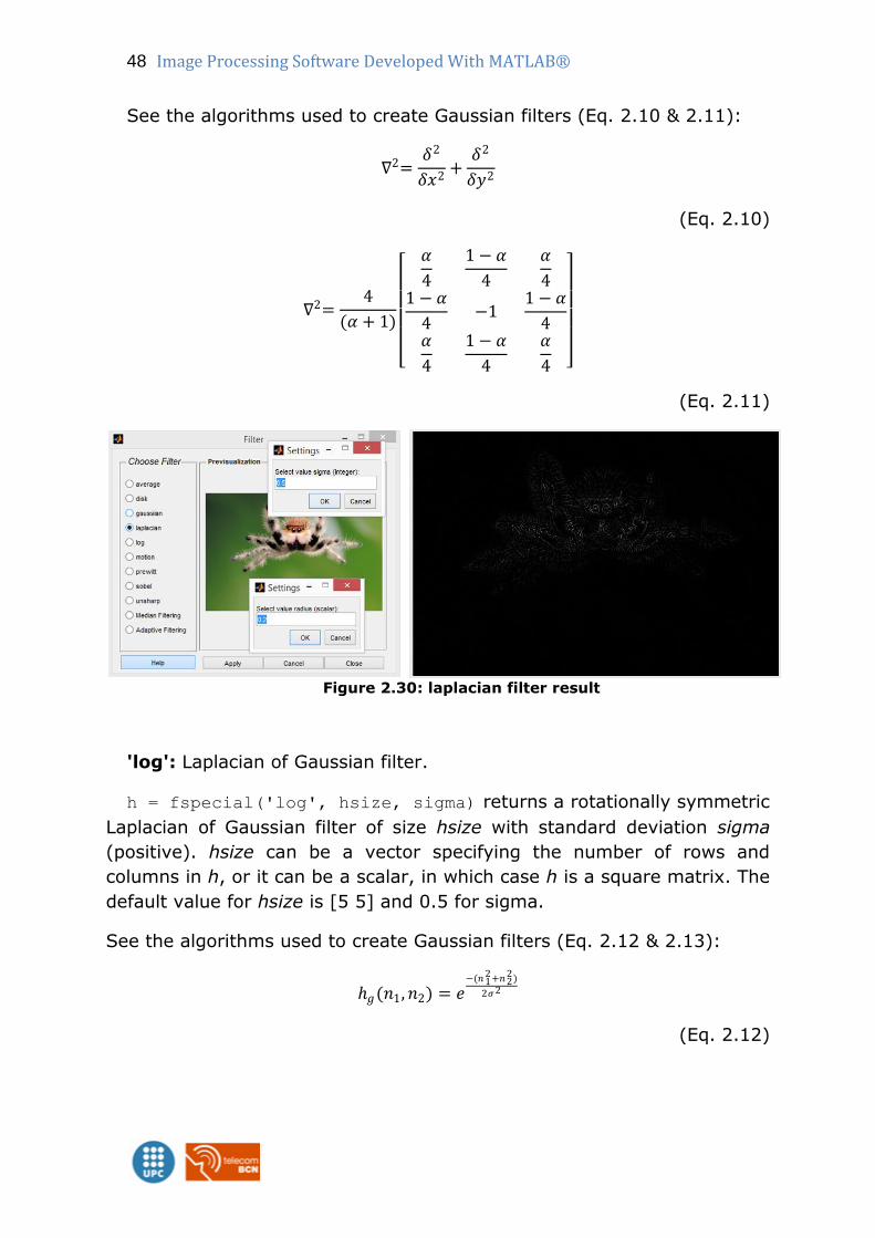
'laplacian': Approximates the two-dimensional Laplacian operator.
h = fspecial('laplacian', alpha) returns a 3-by-3 filter
approximating the shape of the two-dimensional Laplacian operator. The
parameter alpha controls the shape of the Laplacian and must be in the
range 0.0 to 1.0. The default value for alpha is 0.2.
48 Image Processing Software Developed With MATLAB®
See the algorithms used to create Gaussian filters (Eq. 2.10 & 2.11):
∇2=𝛿2
𝛿𝑥2+
𝛿2
𝛿𝑦2
(Eq. 2.10)
∇2=4
(𝛼 + 1)
𝛼
4
1 − 𝛼
4
𝛼
41 − 𝛼
4−1
1 − 𝛼
4𝛼
4
1 − 𝛼
4
𝛼
4
(Eq. 2.11)
Figure 2.30: laplacian filter result
'log': Laplacian of Gaussian filter.
h = fspecial('log', hsize, sigma) returns a rotationally symmetric
Laplacian of Gaussian filter of size hsize with standard deviation sigma
(positive). hsize can be a vector specifying the number of rows and
columns in h, or it can be a scalar, in which case h is a square matrix. The
default value for hsize is [5 5] and 0.5 for sigma.
See the algorithms used to create Gaussian filters (Eq. 2.12 & 2.13):
ℎ𝑔(𝑛1, 𝑛2) = 𝑒−(𝑛1
2+𝑛22)
2𝜎2
(Eq. 2.12)
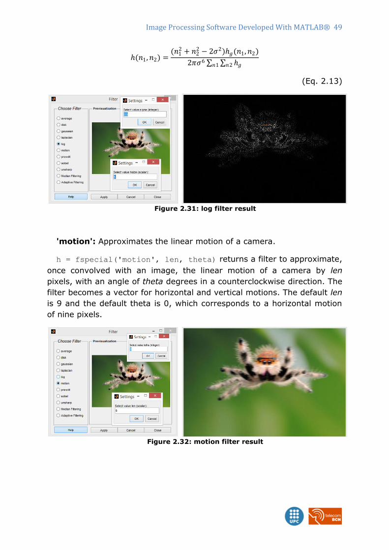
Image Processing Software Developed With MATLAB® 49
ℎ(𝑛1, 𝑛2) =(𝑛1
2 + 𝑛22 − 2𝜎2)ℎ𝑔(𝑛1, 𝑛2)
2𝜋𝜎6 ℎ𝑔𝑛2𝑛1
(Eq. 2.13)
Figure 2.31: log filter result
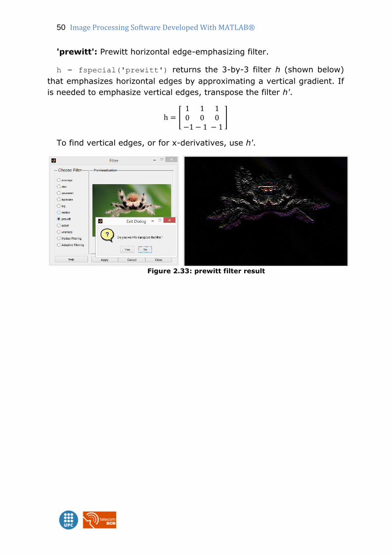
'motion': Approximates the linear motion of a camera.
h = fspecial('motion', len, theta) returns a filter to approximate,
once convolved with an image, the linear motion of a camera by len
pixels, with an angle of theta degrees in a counterclockwise direction. The
filter becomes a vector for horizontal and vertical motions. The default len
is 9 and the default theta is 0, which corresponds to a horizontal motion
of nine pixels.
Figure 2.32: motion filter result
50 Image Processing Software Developed With MATLAB®
'prewitt': Prewitt horizontal edge-emphasizing filter.
h = fspecial('prewitt') returns the 3-by-3 filter h (shown below)
that emphasizes horizontal edges by approximating a vertical gradient. If
is needed to emphasize vertical edges, transpose the filter h'.
h = 1 1 1 0 0 0
−1 − 1 − 1
To find vertical edges, or for x-derivatives, use h'.
Figure 2.33: prewitt filter result
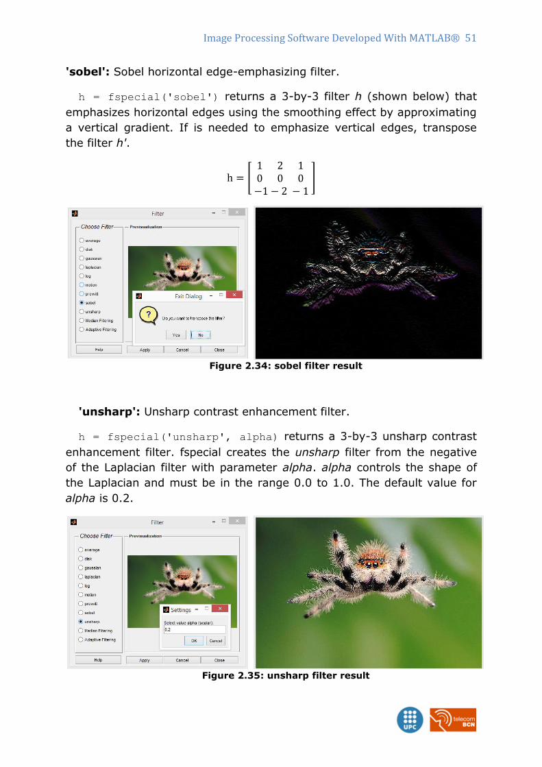
Image Processing Software Developed With MATLAB® 51
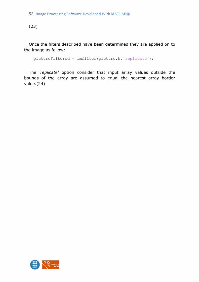
'sobel': Sobel horizontal edge-emphasizing filter.
h = fspecial('sobel') returns a 3-by-3 filter h (shown below) that
emphasizes horizontal edges using the smoothing effect by approximating
a vertical gradient. If is needed to emphasize vertical edges, transpose
the filter h'.
h = 1 2 1 0 0 0
−1 − 2 − 1
Figure 2.34: sobel filter result
'unsharp': Unsharp contrast enhancement filter.
h = fspecial('unsharp', alpha) returns a 3-by-3 unsharp contrast
enhancement filter. fspecial creates the unsharp filter from the negative
of the Laplacian filter with parameter alpha. alpha controls the shape of
the Laplacian and must be in the range 0.0 to 1.0. The default value for
alpha is 0.2.
Figure 2.35: unsharp filter result
52 Image Processing Software Developed With MATLAB®
(23)
Once the filters described have been determined they are applied on to
the image as follow:
pictureFiltered = imfilter(picture,h,'replicate');
The 'replicate' option consider that input array values outside the
bounds of the array are assumed to equal the nearest array border
value.(24)
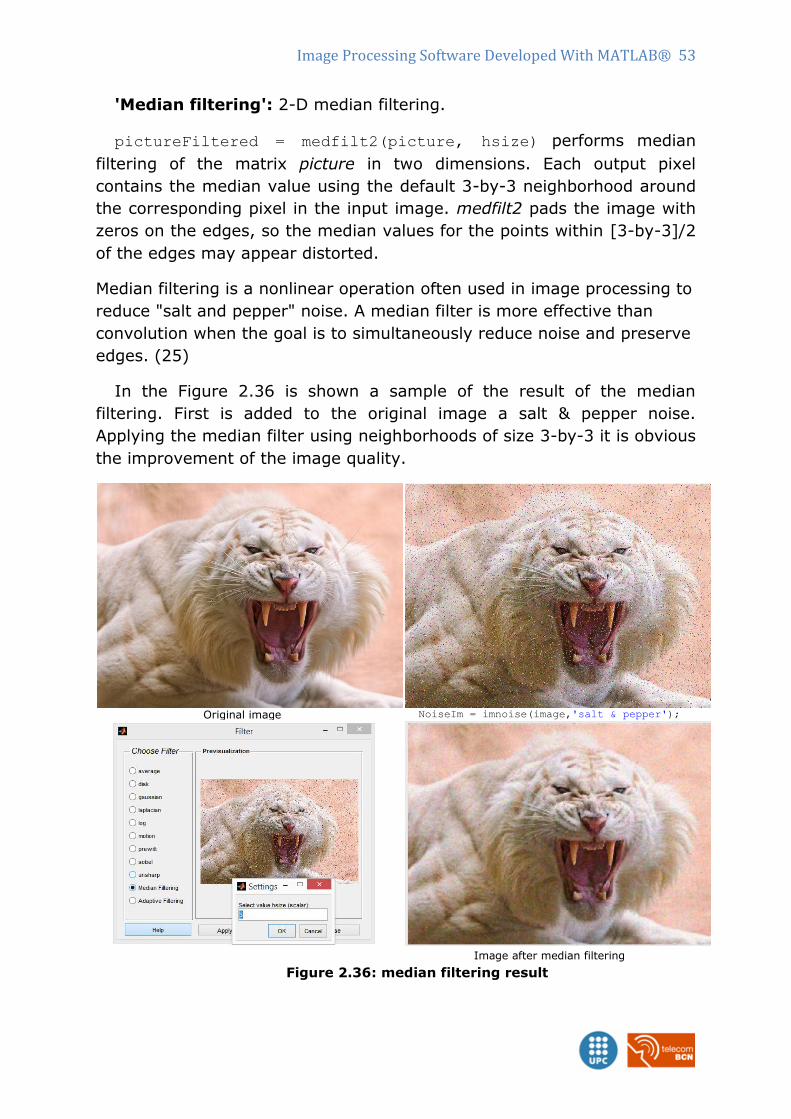
Image Processing Software Developed With MATLAB® 53
'Median filtering': 2-D median filtering.
pictureFiltered = medfilt2(picture, hsize) performs median
filtering of the matrix picture in two dimensions. Each output pixel
contains the median value using the default 3-by-3 neighborhood around
the corresponding pixel in the input image. medfilt2 pads the image with
zeros on the edges, so the median values for the points within [3-by-3]/2
of the edges may appear distorted.
Median filtering is a nonlinear operation often used in image processing to
reduce "salt and pepper" noise. A median filter is more effective than
convolution when the goal is to simultaneously reduce noise and preserve
edges. (25)
In the Figure 2.36 is shown a sample of the result of the median
filtering. First is added to the original image a salt & pepper noise.
Applying the median filter using neighborhoods of size 3-by-3 it is obvious
the improvement of the image quality.
Original image NoiseIm = imnoise(image,'salt & pepper');
Image after median filtering
Figure 2.36: median filtering result
54 Image Processing Software Developed With MATLAB®
'Adaptative filtering': 2-D adaptive noise-removal filtering.
pictureFiltered = wiener2 (picture,[M N],NOISE) filters the
picture using pixel-wise adaptive Wiener filtering, using neighborhoods of
size M-by-N to estimate the local image mean and standard deviation.
The default to 3. The additive noise (Gaussian white noise) power is
assumed to be NOISE.';
See the algorithms used to create Adaptive filter (Eq. 2.14 & 2.15):
wiener2 estimates the local mean and variance around each pixel.
𝜇 =1
𝑁𝑀 a n1, n2
n1 ,n2∈η
(Eq. 2.14)
𝜎2 =1
𝑁𝑀 a2 n1, n2 − μ2
n1 ,n2∈η
(Eq. 2.15)
where η is the N-by-M local neighborhood of each pixel in the
image a. wiener2 then creates a pixelwise Wiener filter using these
estimates
𝑏 n1, n2 = μ +𝜎2 − 𝜐2
𝜎2 a n1, n2 − μ
(Eq. 2.16)
where 𝜐2 is the noise variance. If the noise variance is not
given, wiener2 uses the average of all the local estimated variances.(26)
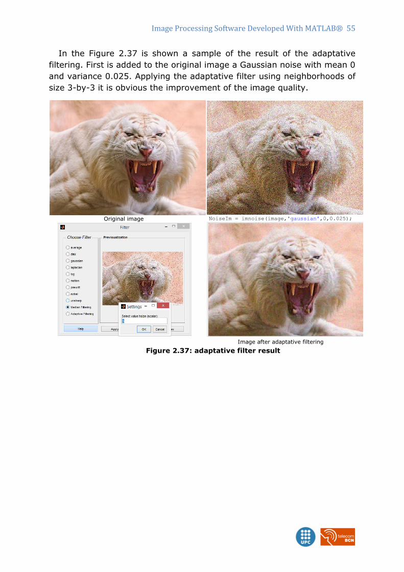
Image Processing Software Developed With MATLAB® 55
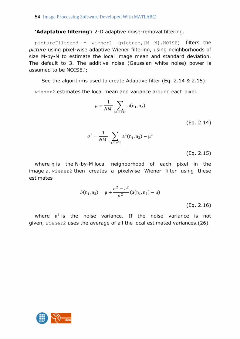
In the Figure 2.37 is shown a sample of the result of the adaptative
filtering. First is added to the original image a Gaussian noise with mean 0
and variance 0.025. Applying the adaptative filter using neighborhoods of
size 3-by-3 it is obvious the improvement of the image quality.
Original image NoiseIm = imnoise(image,'gaussian',0,0.025);
Image after adaptative filtering
Figure 2.37: adaptative filter result
56 Image Processing Software Developed With MATLAB®
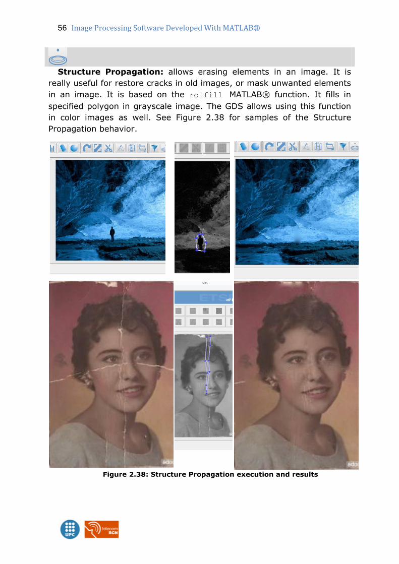
Structure Propagation: allows erasing elements in an image. It is
really useful for restore cracks in old images, or mask unwanted elements
in an image. It is based on the roifill MATLAB® function. It fills in
specified polygon in grayscale image. The GDS allows using this function
in color images as well. See Figure 2.38 for samples of the Structure
Propagation behavior.
Figure 2.38: Structure Propagation execution and results
Image Processing Software Developed With MATLAB® 57
The roifill function smoothly interpolates inward from the pixel
values on the boundary of the polygon by solving Laplace's equation.
J = roifill creates an interactive polygon tool in the current image
in the Workspace, using the mouse to specify the vertices of the polygon.
Uses double-click to add a final vertex to the polygon and close the
polygon. The right-click is used to close the polygon without adding a
vertex. The position of the polygon and individual vertices in the polygon
can be adjusted by clicking and dragging.
To add new vertices, position the pointer along an edge of the polygon
and press the "A" key. The pointer changes shape. It uses left-click to add
a vertex at the specified position.
After positioning and sizing the polygon, fill the region by either double-
clicking over the polygon or choosing Fill Area from the tool's context
menu. The roifill returns J, a version of the image with the region
filled.
To delete the polygon, press Backspace, Escape or Delete, or choose
the Cancel option from the context menu. If the polygon is deleted, all
return values are set to empty.(27)
Although the roifill function just works for grayscale images the GDS
code perform the selection area in the red matrix and replicates the same
area selected for the blue and green. After that the three matrixes are
combined again to get the same effect in a RGB color image.
% over the red matrix is applied the roifill
[x,y,r,J,xi,yi] = roifill(picture(:,:,1));
%the ROI is applied over the green matrix
g = roifill(x,y,picture(:,:,2),xi,yi);
%the ROI is applied over the blue matrix
b = roifill(x,y,picture(:,:,3),xi,yi);
%concatenates the RGB
picture = cat(3, r, g, b);

58 Image Processing Software Developed With MATLAB®
Copy & Paste tools: these tools perform a copy and paste effect
between images. This tool interacts with the Clipboard of the Right
Properties Bar and has a specific behavior as described below.
When running the Copy tool an informative Message box appears:
“The current image is stored for later use. Press Paste button to load it
again.” Press OK button in message The image saved is shown in the
Clipboard axes. When running the Copy tool for the first time the current
image is stored in another variable and shown in the Clipboard of the
Right Properties Bar. This is considered as the main image.
Next appears another informative Message box: “Select the image to
be copied to the current one.” Press OK button in message The Open
Image dialog window appears. The user can open another image or the
last saved version of the main one.
The Figure 2.39 shows the main image in the Workspace and after the
Copy process how the main image is now shown in the Clipboard and the
image to be copied is in the Workspace.
Figure 2.39: Copy tool behavior
The user can work on to the image to be copied, applying whatever
tools or effects as in a main image.
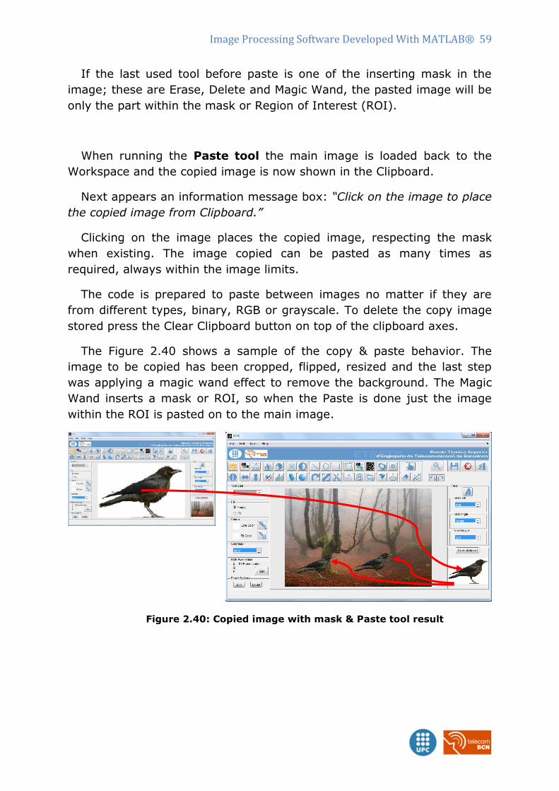
Image Processing Software Developed With MATLAB® 59
If the last used tool before paste is one of the inserting mask in the
image; these are Erase, Delete and Magic Wand, the pasted image will be
only the part within the mask or Region of Interest (ROI).
When running the Paste tool the main image is loaded back to the
Workspace and the copied image is now shown in the Clipboard.
Next appears an information message box: “Click on the image to place
the copied image from Clipboard.”
Clicking on the image places the copied image, respecting the mask
when existing. The image copied can be pasted as many times as
required, always within the image limits.
The code is prepared to paste between images no matter if they are
from different types, binary, RGB or grayscale. To delete the copy image
stored press the Clear Clipboard button on top of the clipboard axes.
The Figure 2.40 shows a sample of the copy & paste behavior. The
image to be copied has been cropped, flipped, resized and the last step
was applying a magic wand effect to remove the background. The Magic
Wand inserts a mask or ROI, so when the Paste is done just the image
within the ROI is pasted on to the main image.
Figure 2.40: Copied image with mask & Paste tool result
60 Image Processing Software Developed With MATLAB®
Next there is a simplified version of the code for the Paste tool with ROI
included: %message box
msg = msgbox('Click on the image…
… to place the copied image');
%wait for the message box to be closed
uiwait(msg);
%Graph input from mouse or cursor to place copied image
[x, y] = ginput(1);
%Main Picture cropped the same size…
…of the whole copied image
pic_crop = imcrop(picture,[x y…
… (size(pic_copy,2)-1) (size(pic_copy,1)-1)]);
%matrix indexing, replacing the mask…
…from the copied image in the cropped
pic_crop(mask)= pic_copy(mask);
% matrix indexing, replacing the cropped…
…picture on to the main Picture
picture(y:y+size(piccrop,1)-1,…
…x:x+size(piccrop,2)-1,:)= pic_crop;
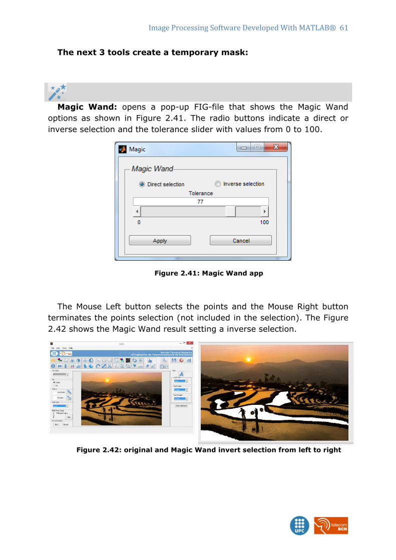
Image Processing Software Developed With MATLAB® 61
The next 3 tools create a temporary mask:
Magic Wand: opens a pop-up FIG-file that shows the Magic Wand
options as shown in Figure 2.41. The radio buttons indicate a direct or
inverse selection and the tolerance slider with values from 0 to 100.
Figure 2.41: Magic Wand app
The Mouse Left button selects the points and the Mouse Right button
terminates the points selection (not included in the selection). The Figure
2.42 shows the Magic Wand result setting a inverse selection.
Figure 2.42: original and Magic Wand invert selection from left to right
62 Image Processing Software Developed With MATLAB®
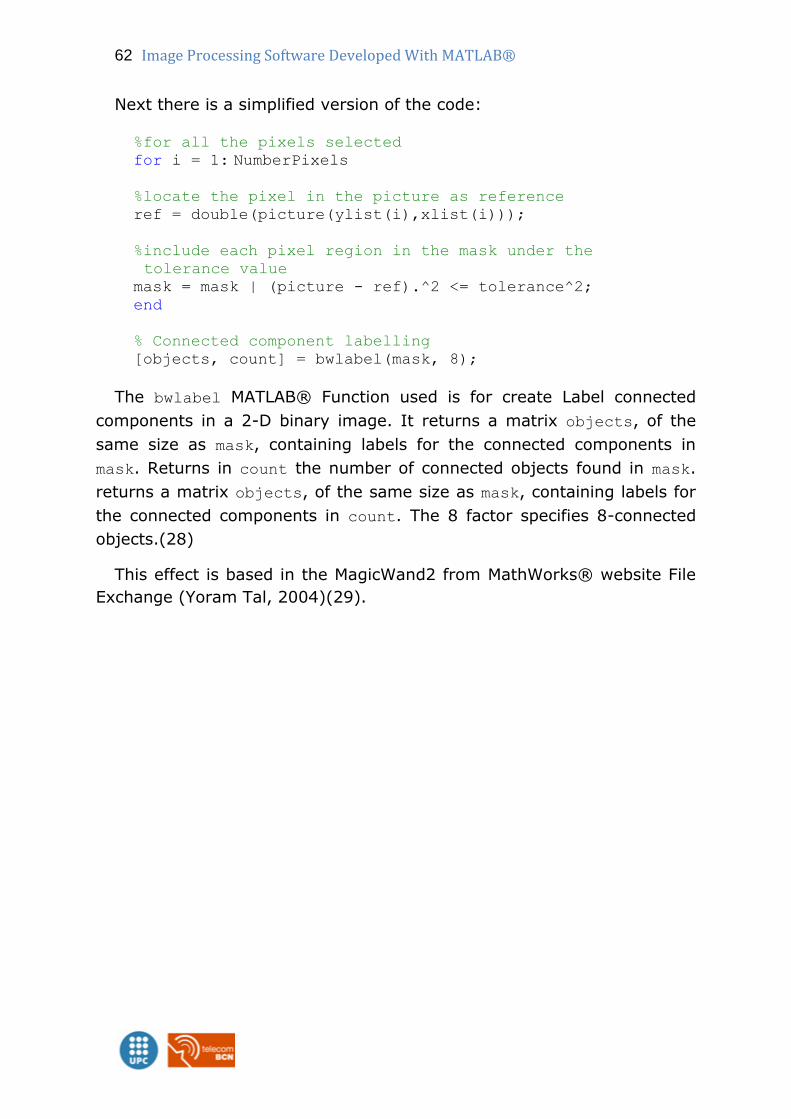
Next there is a simplified version of the code:
%for all the pixels selected
for i = 1: NumberPixels
%locate the pixel in the picture as reference
ref = double(picture(ylist(i),xlist(i)));
%include each pixel region in the mask under the
tolerance value
mask = mask | (picture - ref).^2 <= tolerance^2;
end
% Connected component labelling
[objects, count] = bwlabel(mask, 8);
The bwlabel MATLAB® Function used is for create Label connected
components in a 2-D binary image. It returns a matrix objects, of the
same size as mask, containing labels for the connected components in
mask. Returns in count the number of connected objects found in mask.
returns a matrix objects, of the same size as mask, containing labels for
the connected components in count. The 8 factor specifies 8-connected
objects.(28)
This effect is based in the MagicWand2 from MathWorks® website File
Exchange (Yoram Tal, 2004)(29).
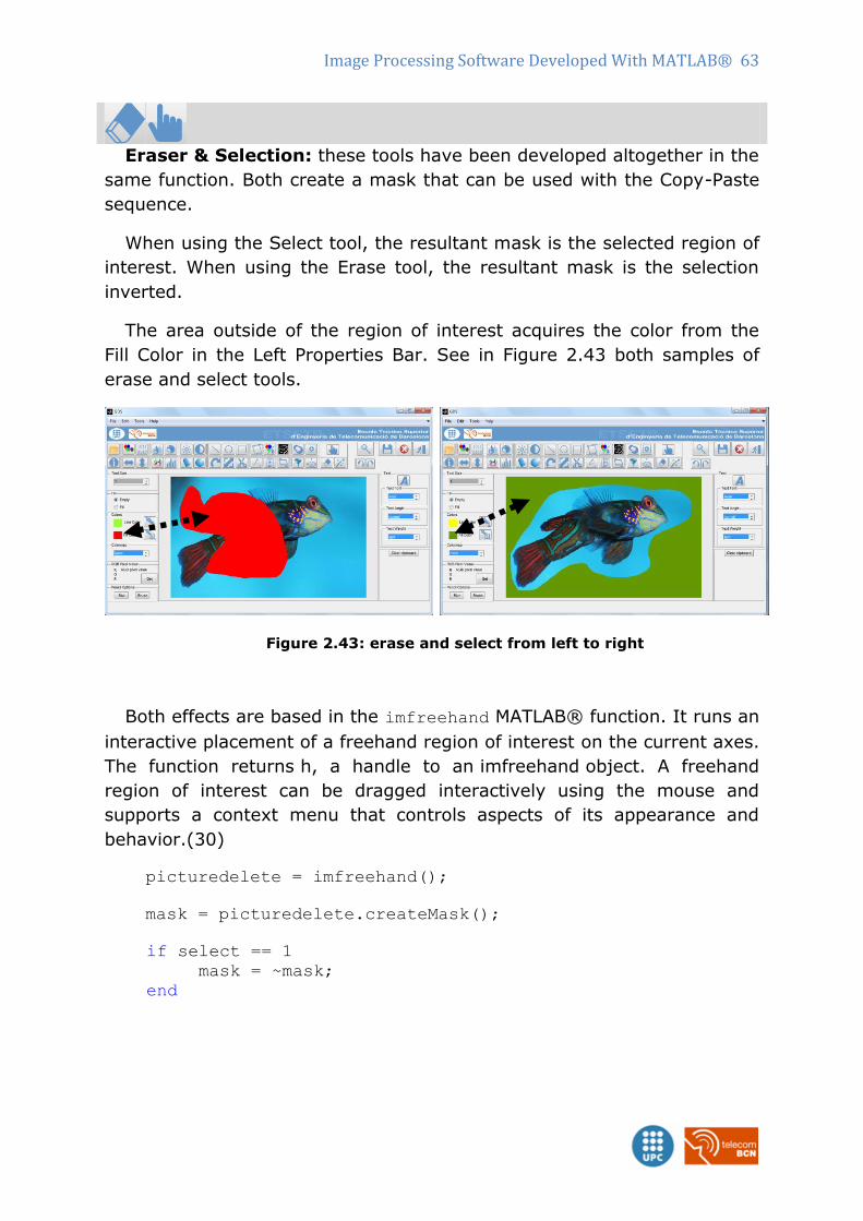
Image Processing Software Developed With MATLAB® 63
Eraser & Selection: these tools have been developed altogether in the
same function. Both create a mask that can be used with the Copy-Paste
sequence.
When using the Select tool, the resultant mask is the selected region of
interest. When using the Erase tool, the resultant mask is the selection
inverted.
The area outside of the region of interest acquires the color from the
Fill Color in the Left Properties Bar. See in Figure 2.43 both samples of
erase and select tools.
Figure 2.43: erase and select from left to right
Both effects are based in the imfreehand MATLAB® function. It runs an
interactive placement of a freehand region of interest on the current axes.
The function returns h, a handle to an imfreehand object. A freehand
region of interest can be dragged interactively using the mouse and
supports a context menu that controls aspects of its appearance and
behavior.(30)
picturedelete = imfreehand();
mask = picturedelete.createMask();
if select == 1 mask = ~mask; end
64 Image Processing Software Developed With MATLAB®
2.3.2 Left Properties Bar
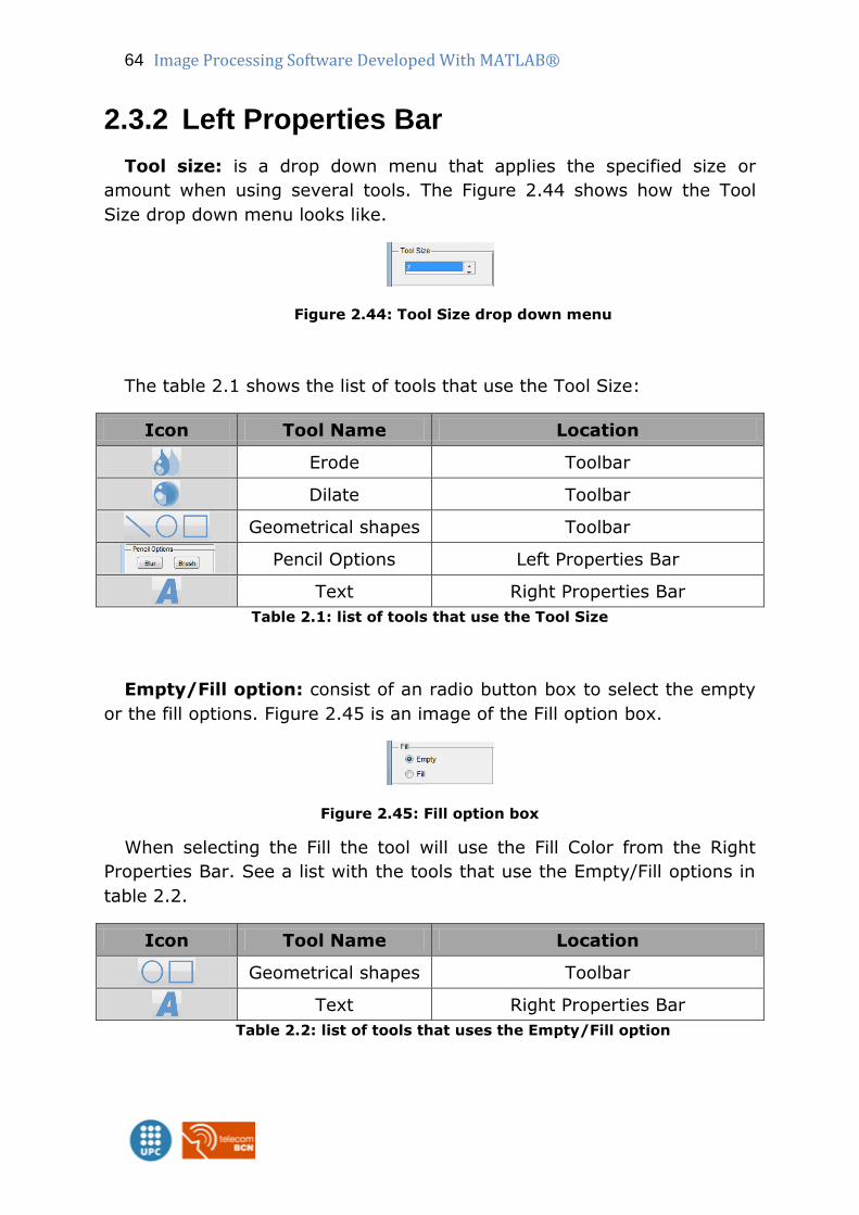
Tool size: is a drop down menu that applies the specified size or
amount when using several tools. The Figure 2.44 shows how the Tool
Size drop down menu looks like.
Figure 2.44: Tool Size drop down menu
The table 2.1 shows the list of tools that use the Tool Size:
Icon Tool Name Location
Erode Toolbar
Dilate Toolbar
Geometrical shapes Toolbar
Pencil Options Left Properties Bar
Text Right Properties Bar
Table 2.1: list of tools that use the Tool Size
Empty/Fill option: consist of an radio button box to select the empty
or the fill options. Figure 2.45 is an image of the Fill option box.
Figure 2.45: Fill option box
When selecting the Fill the tool will use the Fill Color from the Right
Properties Bar. See a list with the tools that use the Empty/Fill options in
table 2.2.
Icon Tool Name Location
Geometrical shapes Toolbar
Text Right Properties Bar
Table 2.2: list of tools that uses the Empty/Fill option
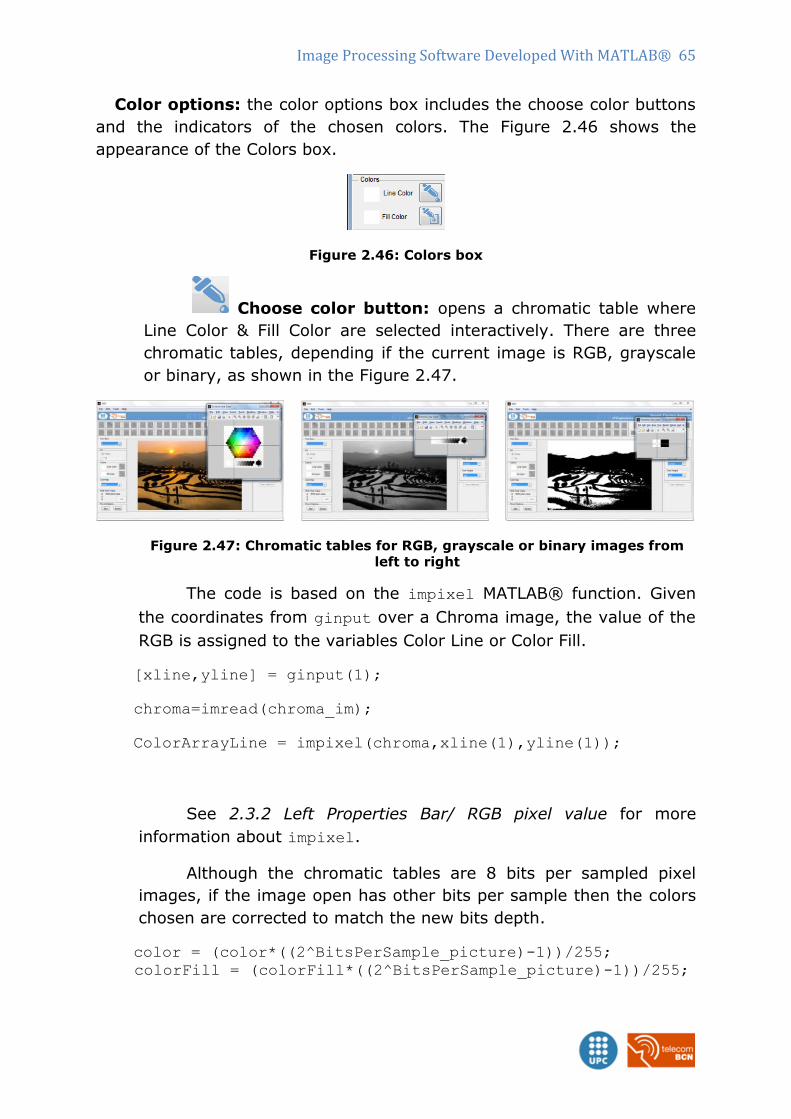
Image Processing Software Developed With MATLAB® 65
Color options: the color options box includes the choose color buttons
and the indicators of the chosen colors. The Figure 2.46 shows the
appearance of the Colors box.
Figure 2.46: Colors box
Choose color button: opens a chromatic table where
Line Color & Fill Color are selected interactively. There are three
chromatic tables, depending if the current image is RGB, grayscale
or binary, as shown in the Figure 2.47.
Figure 2.47: Chromatic tables for RGB, grayscale or binary images from
left to right
The code is based on the impixel MATLAB® function. Given
the coordinates from ginput over a Chroma image, the value of the
RGB is assigned to the variables Color Line or Color Fill.
[xline,yline] = ginput(1);
chroma=imread(chroma_im);
ColorArrayLine = impixel(chroma,xline(1),yline(1));
See 2.3.2 Left Properties Bar/ RGB pixel value for more
information about impixel.
Although the chromatic tables are 8 bits per sampled pixel
images, if the image open has other bits per sample then the colors
chosen are corrected to match the new bits depth.
color = (color*((2^BitsPerSample_picture)-1))/255; colorFill = (colorFill*((2^BitsPerSample_picture)-1))/255;
66 Image Processing Software Developed With MATLAB®
Choose color image button: let‟s interactively select
the Line Color & Fill Color in the current image.
The code is based on the impixel MATLAB® function. Given
the coordinates from ginput over the current image in the
Workspace, the value of the RGB is assigned to the variables Color
Line or Color Fill.
[xline,yline] = ginput(2);
ColorArrayLine = impixel(picture,xline(1),yline(1));
ColorArrayFill = impixel(picture,xline(2),yline(2));
See 2.3.2 Left Properties Bar/ RGB pixel value for more
information about impixel.
Line Color & Fill Color: shows the current colors selected
through the Choose Color tools. Both are white by default. Figure
2.48 shows the color indicators appearance.
Figure 2.48: Line Color & Fill Color indicators
The Line Color is used in the tools listed in the table 2.3.
Icon Tool Name Location
Geometrical shapes Toolbar
Pencil Options / Brush Left Properties Bar
Text Right Properties Bar
Table 2.3: tools that use the Line Color
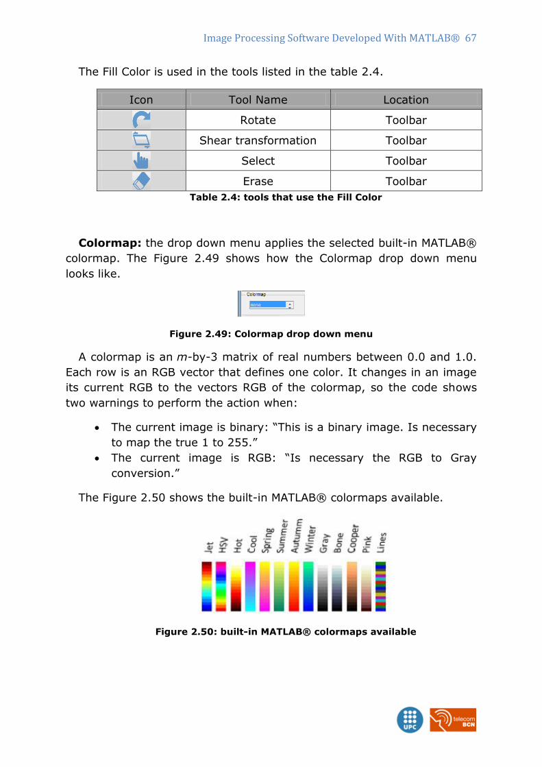
Image Processing Software Developed With MATLAB® 67
The Fill Color is used in the tools listed in the table 2.4.
Icon Tool Name Location
Rotate Toolbar
Shear transformation Toolbar
Select Toolbar
Erase Toolbar
Table 2.4: tools that use the Fill Color
Colormap: the drop down menu applies the selected built-in MATLAB®
colormap. The Figure 2.49 shows how the Colormap drop down menu
looks like.
Figure 2.49: Colormap drop down menu
A colormap is an m-by-3 matrix of real numbers between 0.0 and 1.0.
Each row is an RGB vector that defines one color. It changes in an image
its current RGB to the vectors RGB of the colormap, so the code shows
two warnings to perform the action when:
The current image is binary: “This is a binary image. Is necessary
to map the true 1 to 255.”
The current image is RGB: “Is necessary the RGB to Gray
conversion.”
The Figure 2.50 shows the built-in MATLAB® colormaps available.
Figure 2.50: built-in MATLAB® colormaps available
68 Image Processing Software Developed With MATLAB®
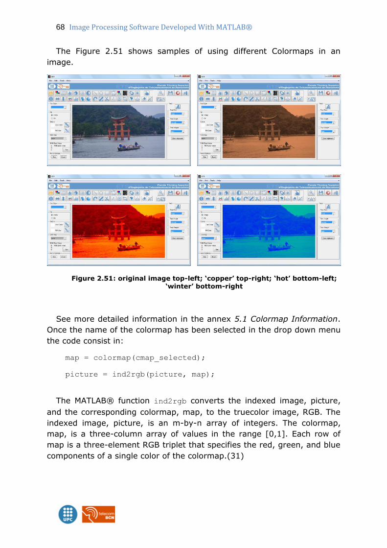
The Figure 2.51 shows samples of using different Colormaps in an
image.
Figure 2.51: original image top-left; ‘copper’ top-right; ‘hot’ bottom-left;
‘winter’ bottom-right
See more detailed information in the annex 5.1 Colormap Information.
Once the name of the colormap has been selected in the drop down menu
the code consist in:
map = colormap(cmap_selected);
picture = ind2rgb(picture, map);
The MATLAB® function ind2rgb converts the indexed image, picture,
and the corresponding colormap, map, to the truecolor image, RGB. The
indexed image, picture, is an m-by-n array of integers. The colormap,
map, is a three-column array of values in the range [0,1]. Each row of
map is a three-element RGB triplet that specifies the red, green, and blue
components of a single color of the colormap.(31)
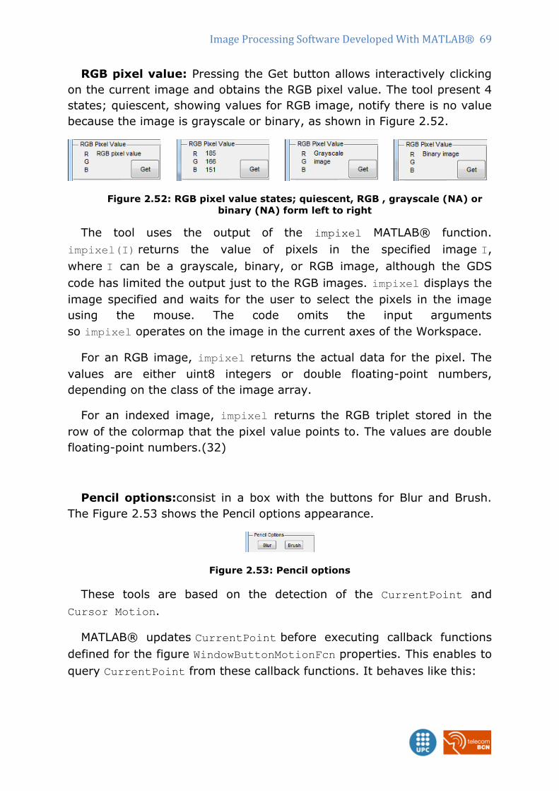
Image Processing Software Developed With MATLAB® 69
RGB pixel value: Pressing the Get button allows interactively clicking
on the current image and obtains the RGB pixel value. The tool present 4
states; quiescent, showing values for RGB image, notify there is no value
because the image is grayscale or binary, as shown in Figure 2.52.
Figure 2.52: RGB pixel value states; quiescent, RGB , grayscale (NA) or
binary (NA) form left to right
The tool uses the output of the impixel MATLAB® function.
impixel(I) returns the value of pixels in the specified image I,
where I can be a grayscale, binary, or RGB image, although the GDS
code has limited the output just to the RGB images. impixel displays the
image specified and waits for the user to select the pixels in the image
using the mouse. The code omits the input arguments
so impixel operates on the image in the current axes of the Workspace.
For an RGB image, impixel returns the actual data for the pixel. The
values are either uint8 integers or double floating-point numbers,
depending on the class of the image array.
For an indexed image, impixel returns the RGB triplet stored in the
row of the colormap that the pixel value points to. The values are double
floating-point numbers.(32)
Pencil options:consist in a box with the buttons for Blur and Brush.
The Figure 2.53 shows the Pencil options appearance.
Figure 2.53: Pencil options
These tools are based on the detection of the CurrentPoint and
Cursor Motion.
MATLAB® updates CurrentPoint before executing callback functions
defined for the figure WindowButtonMotionFcn properties. This enables to
query CurrentPoint from these callback functions. It behaves like this:
70 Image Processing Software Developed With MATLAB®
When defining a callback function for the
WindowButtonMotionFcn property, then MATLAB updates the
CurrentPoint property only when the user presses the mouse
button within the figure window.
When defining a callback function for the
WindowButtonMotionFcn property, then MATLAB updates the
CurrentPoint property just before executing the callback.
The WindowButtonMotionFcn property executes only within the
figure window, unless the user presses the mouse button within
the figure and keeps the mouse button down while moving the
pointer around the screen. In this case, the function executes
(and MATLAB updates the CurrentPoint property) anywhere on
the screen until the user releases the mouse button.
When defining a callback function for the WindowButtonUpFcn
property, then MATLAB updates the CurrentPoint property just
before executing the callback.
If adding a uicontrol or uitable component to the figure, then
MATLAB® updates the CurrentPoint property when the user right-clicks
the component, or when they left-click the component while
the Enable property of that component is 'off' or 'inactive'.
In some situations (such as when the WindowButtonMotionFcn callback
takes a long time to execute and the user moves the pointer very
rapidly), the CurrentPoint property might not reflect the actual location
of the pointer, but rather the location at the time when the
WindowButtonMotionFcn callback began execution.(33)
Blur: follows the cursor movement when pressing the left
mouse button performing a blurring effect on to the image in the
Workspace. The Tool Size selected from the Left Properties Bar sets
the square area affected for the blurring.
The common application for this tool is to minimize pixelated
regions in pictures. As an example the Figure 2.54 shows a bad
quality picture that presents the typical pixelated region especially
visible on the edges. Using the blur tool following the lines the
pixelation can be satisfactorily smoothen, improving the image
visualization and printing. The Zoom can be combined with the blur
effect to achieve higher precision in the image correction.
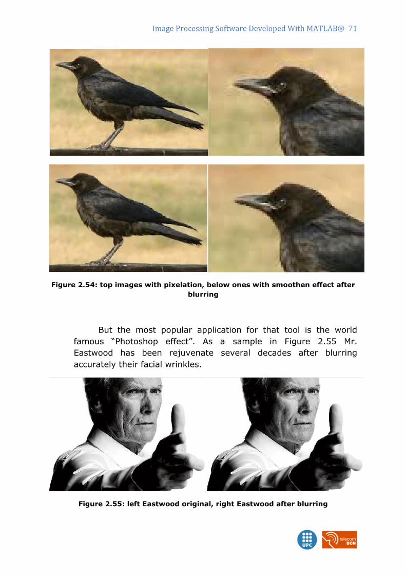
Image Processing Software Developed With MATLAB® 71
Figure 2.54: top images with pixelation, below ones with smoothen effect after
blurring
But the most popular application for that tool is the world
famous “Photoshop effect”. As a sample in Figure 2.55 Mr.
Eastwood has been rejuvenate several decades after blurring
accurately their facial wrinkles.
Figure 2.55: left Eastwood original, right Eastwood after blurring
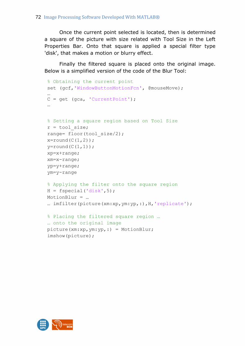
72 Image Processing Software Developed With MATLAB®
Once the current point selected is located, then is determined
a square of the picture with size related with Tool Size in the Left
Properties Bar. Onto that square is applied a special filter type
'disk', that makes a motion or blurry effect.
Finally the filtered square is placed onto the original image.
Below is a simplified version of the code of the Blur Tool:
% Obtaining the current point
set (gcf,'WindowButtonMotionFcn', @mouseMove);
…
C = get (gca, 'CurrentPoint');
…
% Setting a square region based on Tool Size
r = tool_size;
range= floor(tool_size/2);
x=round(C(1,2));
y=round(C(1,1));
xp=x+range;
xm=x-range;
yp=y+range;
ym=y-range
% Applying the filter onto the square region
H = fspecial('disk',5);
MotionBlur = …
… imfilter(picture(xm:xp,ym:yp,:),H,'replicate');
% Placing the filtered square region …
… onto the original image
picture(xm:xp,ym:yp,:) = MotionBlur;
imshow(picture);
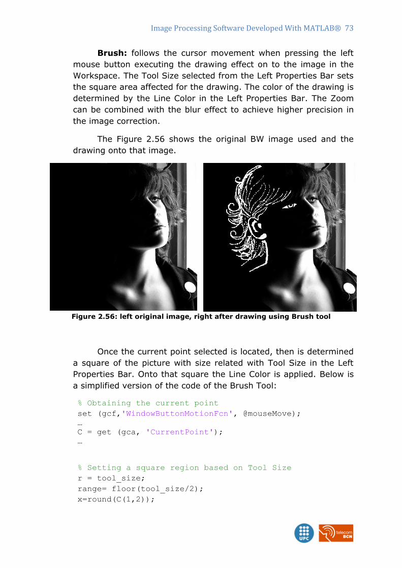
Image Processing Software Developed With MATLAB® 73
Brush: follows the cursor movement when pressing the left
mouse button executing the drawing effect on to the image in the
Workspace. The Tool Size selected from the Left Properties Bar sets
the square area affected for the drawing. The color of the drawing is
determined by the Line Color in the Left Properties Bar. The Zoom
can be combined with the blur effect to achieve higher precision in
the image correction.
The Figure 2.56 shows the original BW image used and the
drawing onto that image.
Figure 2.56: left original image, right after drawing using Brush tool
Once the current point selected is located, then is determined
a square of the picture with size related with Tool Size in the Left
Properties Bar. Onto that square the Line Color is applied. Below is
a simplified version of the code of the Brush Tool:
% Obtaining the current point
set (gcf,'WindowButtonMotionFcn', @mouseMove);
…
C = get (gca, 'CurrentPoint');
…
% Setting a square region based on Tool Size
r = tool_size;
range= floor(tool_size/2);
x=round(C(1,2));
74 Image Processing Software Developed With MATLAB®
y=round(C(1,1));
xp=x+range;
xm=x-range;
yp=y+range;
ym=y-range
% Applying the color over the square region …
… on the RGB image
picture(xxm:xxp,yym:yyp,1)= color(1);
picture(xxm:xxp,yym:yyp,2)= color(2);
picture(xxm:xxp,yym:yyp,3)= color(3);
imshow(picture);
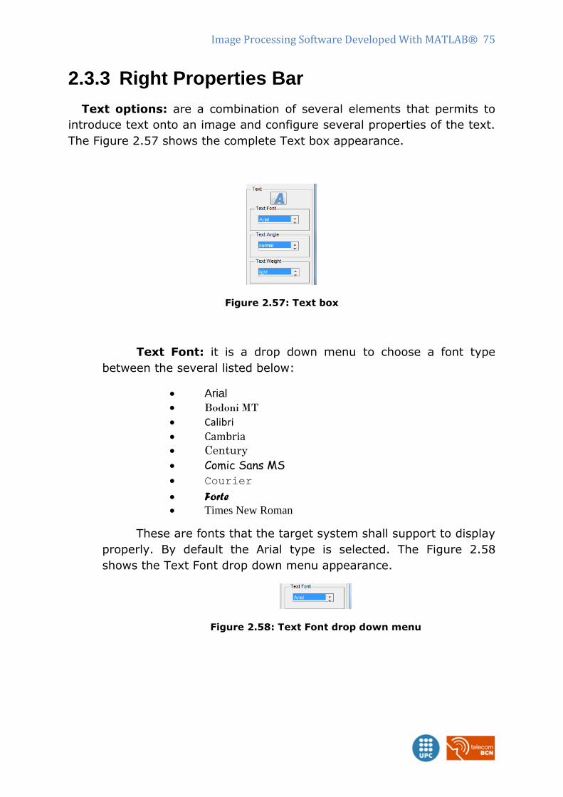
Image Processing Software Developed With MATLAB® 75
2.3.3 Right Properties Bar
Text options: are a combination of several elements that permits to
introduce text onto an image and configure several properties of the text.
The Figure 2.57 shows the complete Text box appearance.
Figure 2.57: Text box
Text Font: it is a drop down menu to choose a font type
between the several listed below:
Arial
Bodoni MT
Calibri
Cambria Century
Comic Sans MS Courier
Forte
Times New Roman
These are fonts that the target system shall support to display
properly. By default the Arial type is selected. The Figure 2.58
shows the Text Font drop down menu appearance.
Figure 2.58: Text Font drop down menu
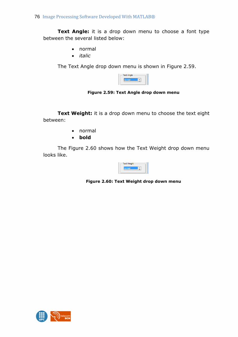
76 Image Processing Software Developed With MATLAB®
Text Angle: it is a drop down menu to choose a font type
between the several listed below:
normal
italic
The Text Angle drop down menu is shown in Figure 2.59.
Figure 2.59: Text Angle drop down menu
Text Weight: it is a drop down menu to choose the text eight
between:
normal
bold
The Figure 2.60 shows how the Text Weight drop down menu
looks like.
Figure 2.60: Text Weight drop down menu
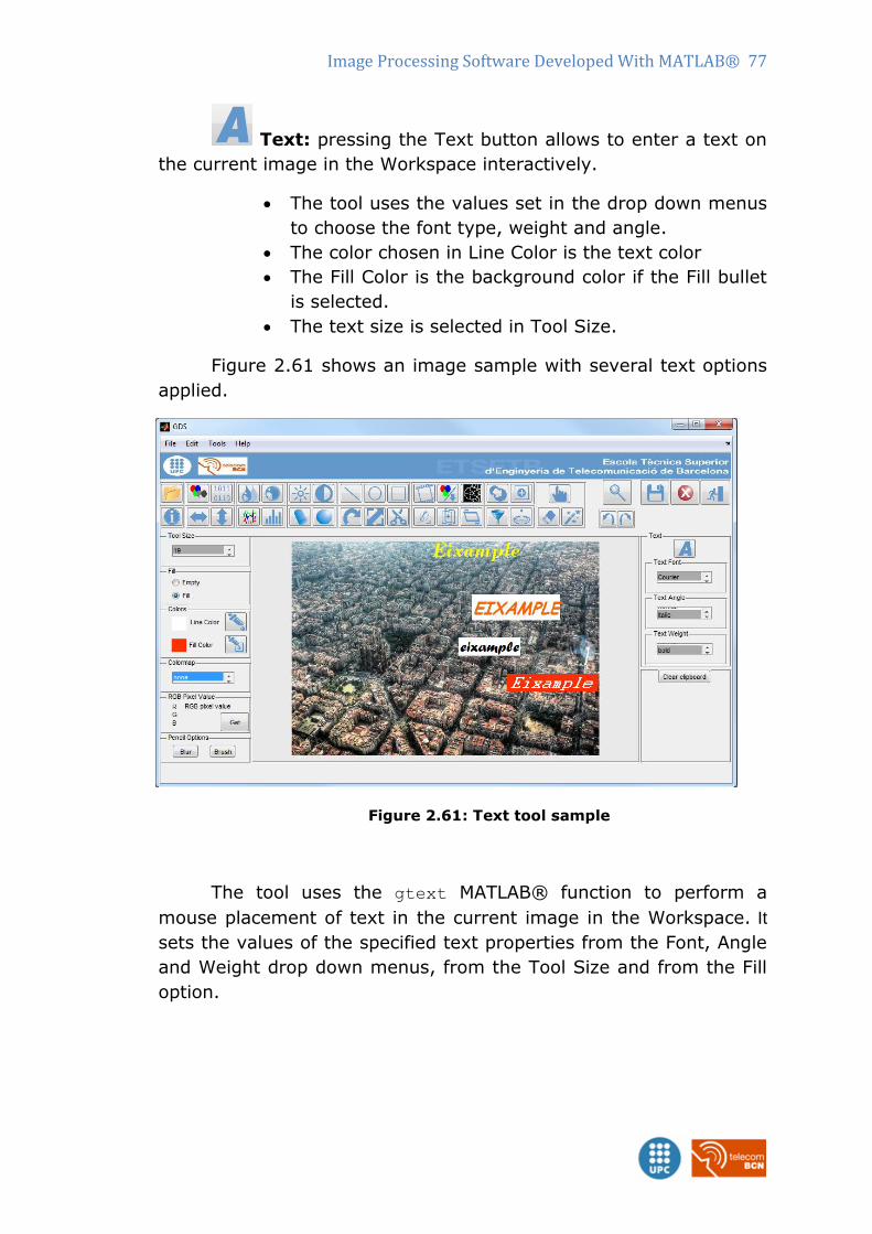
Image Processing Software Developed With MATLAB® 77
Text: pressing the Text button allows to enter a text on
the current image in the Workspace interactively.
The tool uses the values set in the drop down menus
to choose the font type, weight and angle.
The color chosen in Line Color is the text color
The Fill Color is the background color if the Fill bullet
is selected.
The text size is selected in Tool Size.
Figure 2.61 shows an image sample with several text options
applied.
Figure 2.61: Text tool sample
The tool uses the gtext MATLAB® function to perform a
mouse placement of text in the current image in the Workspace. It
sets the values of the specified text properties from the Font, Angle
and Weight drop down menus, from the Tool Size and from the Fill
option.
78 Image Processing Software Developed With MATLAB®
The Text to be written is introduced through an input dialog
window. A simplified extract of the Text tool code is shown below:
answer = inputdlg('Type the text','Settings',1);
switch (fillshape)
case 0%Fill bullet deselected
gtext(answer,'FontSize',tool_size,'FontName',…
…Font_Name_selected,'FontAngle',Font_Angle_selected,…
…'FontWeight',Font_Weight_selected,'Color',color);
case 1%Fill bullet selected
gtext(answer,'FontSize',tool_size,'FontName',…
…Font_Name_selected,'FontAngle',Font_Angle_selected,…
…'FontWeight',Font_Weight_selected,'Color',…
…color,'BackgroundColor',colorFill);
end
Clipboard: the clipboard axes show a stored image when using the
Copy/Paste functions:
Using the Copy tool: the main picture in the Worskpace axes is
saved in the Clipboard axes.
Using Paste option: the main picture is restored to the
Workspace axes and the image to be pasted is saved in the
clipboard axes.
The Clear Clipboard button erases any image saved in the clipboard
axes.
See section 2.3.1 Toolbar/ Copy & Paste for more information.
Image Processing Software Developed With MATLAB® 79
2.3.4 Zoom
Zoom: it uses the zoom MATLAB® function. Turns on interactive
zooming. When interactive zooming is enabled in a figure, pressing a
mouse button while the cursor is within an axes zooms into the point or
out from the point beneath the mouse. Zooming changes the axes limits.
When using zoom mode:
Zoom in by positioning the mouse cursor where you want the
center of the plot to be and either:
o Press the mouse button or
o Rotate the mouse scroll wheel away from you (upward).
Zoom out by positioning the mouse cursor where wanted the
center of the plot to be and either:
o Simultaneously press Shift and the mouse button, or
o Rotate the mouse scroll wheel toward you (downward).
Each mouse click or scroll wheel click zooms in or out by a factor of 2.
Clicking and dragging over an axes when zooming in is enabled draws a
rubberband box. When you release the mouse button, the axes zoom in
to the region enclosed by the rubberband box.
Double-clicking over an axes returns the axes to its initial zoom setting
in both zoom-in and zoom-out modes.(34)
The tool is implemented with a toggle button, so when it is pressed the
zoom options are available onto the current image. When deactivate the
toggle the zoom is restored.
The new image limits during the zooming are preserved if any other
tool is activated. This tool allows for example to work with more precision
when using the Pencil options in the Left Properties Bar.
80 Image Processing Software Developed With MATLAB®
Next there is extract of the code for the Zoom tool:
% --- Executes on button press in togglebuttonzooom.
function togglebuttonZoom_Callback(hObject, eventdata, handles)
global ZoomValue
global picture
ZoomValue = get(gcbo,'Value'); %returns state of togglebuttonzooom
if ZoomValue == 1 %togglebutton is pressed
h = zoom;
set(h,'ActionPostCallback',@mypostcallback);
set(h,'Enable','on');
else
set(gca,'xlim',[1 size(picture,2)])
set(gca,'ylim',[1 size(picture,1)])
zoom off
end
function mypostcallback(obj,evd)
global newXLim
global newYLim
%new image limits
newXLim = get(evd.Axes,'XLim');
newYLim = get(evd.Axes,'YLim');
Image Processing Software Developed With MATLAB® 81
2.3.5 Save options
There are two options to save the image on the Workspace, the Save
and the Save As. This last one is only available using the Menu; File/ Save
As.
Save: performs an overwriting of the current image on the Workspace.
A dialog pop up ask the user if really wants to overwrite the image, and
when affirmative executes the imwrite MATLAB® function.
imwrite(A,filename) writes image data A to the file specified by
filename, inferring the file format from the extension. imwrite creates the
new file in your current folder. The bit depth of the output image depends
on the data type of A and the file format. For most formats:
If A is of data type uint8, then imwrite outputs 8-bit values.
If A is of data type uint16 and the output file format supports 16-
bit data (JPEG, PNG, and TIFF), then imwrite outputs 16-bit
values. If the output file format does not support 16-bit data,
then imwrite returns an error.
If A is a grayscale or RGB color image of data type double or
single, then imwrite assumes that the dynamic range is [0,1]
and automatically scales the data by 255 before writing it to the
file as 8-bit values. If the data in A is single, convert A to double
before writing to a GIF or TIFF file.
If A is of data type logical, then imwrite assumes that the data is
a binary image and writes it to the file with a bit depth of 1, if the
format allows it. BMP, PNG, or TIFF formats accept binary images
as input arrays.
If A contains indexed image data, the user shall additionally
specify the map input argument, although the GDS code does not
have this option implemented.
(35)
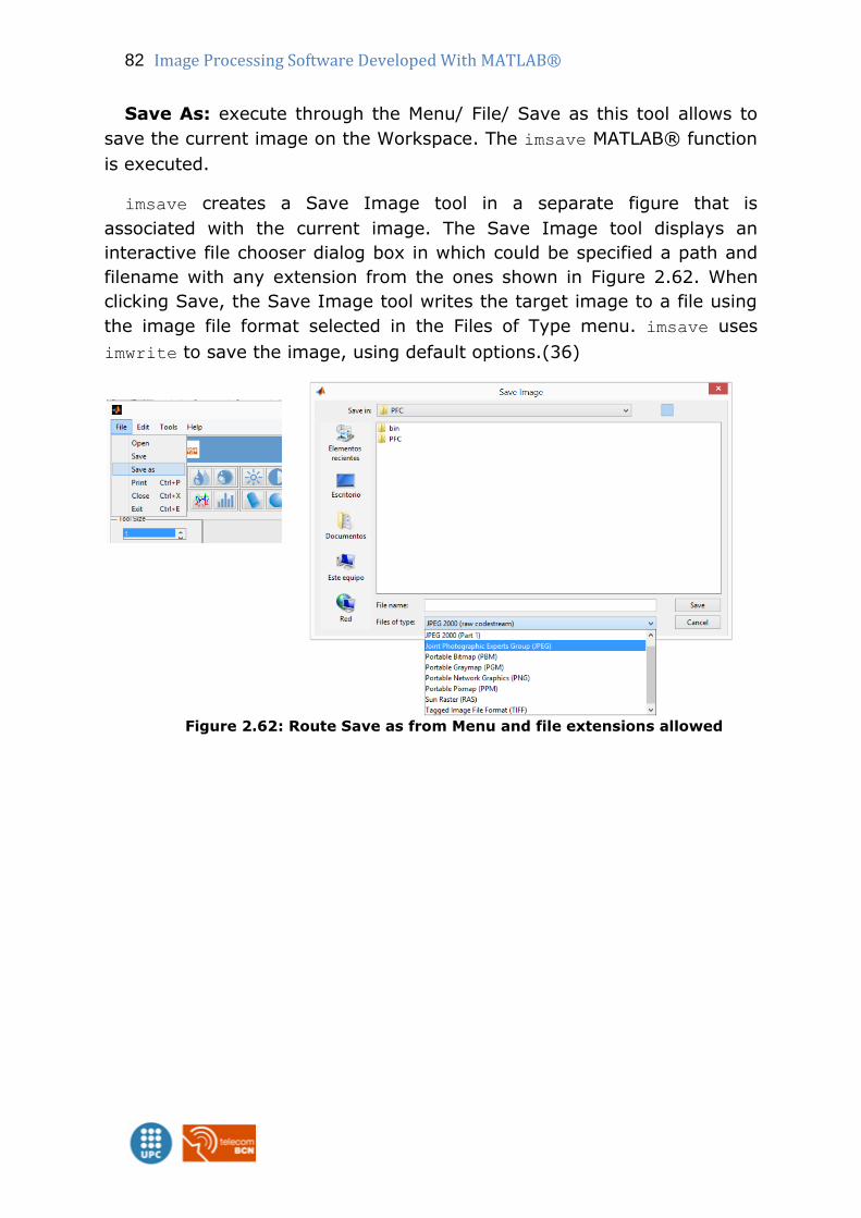
82 Image Processing Software Developed With MATLAB®
Save As: execute through the Menu/ File/ Save as this tool allows to
save the current image on the Workspace. The imsave MATLAB® function
is executed.
imsave creates a Save Image tool in a separate figure that is
associated with the current image. The Save Image tool displays an
interactive file chooser dialog box in which could be specified a path and
filename with any extension from the ones shown in Figure 2.62. When
clicking Save, the Save Image tool writes the target image to a file using
the image file format selected in the Files of Type menu. imsave uses
imwrite to save the image, using default options.(36)
Figure 2.62: Route Save as from Menu and file extensions allowed
Image Processing Software Developed With MATLAB® 83
2.4 File format compatibility
The GDS uses the imread function for reading an image from graphics
file. This MATLAB® function reads a grayscale or color image from the file
specified by the string filename.
[...] = imread(filename)
The imread function is compatible for the next specific formats, listed in
alphabetical order by format name.
BMP — Windows Bitmap
CUR — Cursor File
GIF — Graphics Interchange Format
HDF4 — Hierarchical Data Format
ICO — Icon File
JPEG — Joint Photographic Experts Group
JPEG 2000 — Joint Photographic Experts Group 2000
PBM — Portable Bitmap
PCX — Windows Paintbrush
PGM — Portable Graymap
PNG — Portable Network Graphics
PPM — Portable Pixmap
RAS — Sun Raster
TIFF — Tagged Image File Format
XWD — X Window Dump
More detailed information in the annex 5.2 Format-Specific Information.
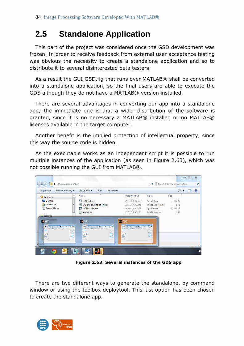
84 Image Processing Software Developed With MATLAB®
2.5 Standalone Application
This part of the project was considered once the GSD development was
frozen. In order to receive feedback from external user acceptance testing
was obvious the necessity to create a standalone application and so to
distribute it to several disinterested beta testers.
As a result the GUI GSD.fig that runs over MATLAB® shall be converted
into a standalone application, so the final users are able to execute the
GDS although they do not have a MATLAB® version installed.
There are several advantages in converting our app into a standalone
app; the immediate one is that a wider distribution of the software is
granted, since it is no necessary a MATLAB® installed or no MATLAB®
licenses available in the target computer.
Another benefit is the implied protection of intellectual property, since
this way the source code is hidden.
As the executable works as an independent script it is possible to run
multiple instances of the application (as seen in Figure 2.63), which was
not possible running the GUI from MATLAB®.
Figure 2.63: Several instances of the GDS app
There are two different ways to generate the standalone, by command
window or using the toolbox deploytool. This last option has been chosen
to create the standalone app.
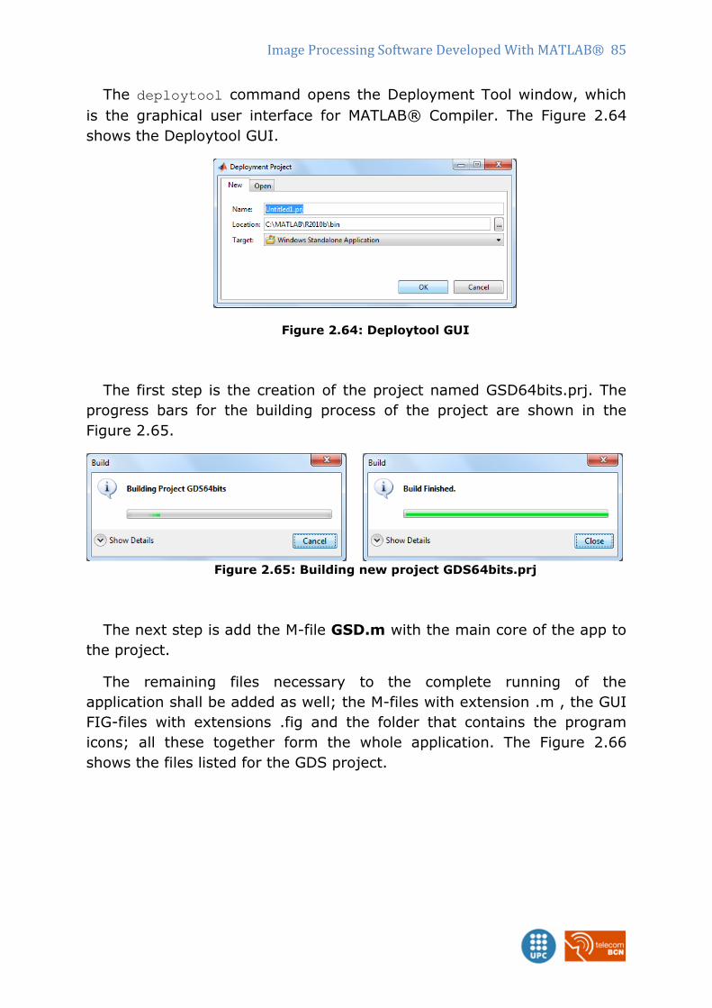
Image Processing Software Developed With MATLAB® 85
The deploytool command opens the Deployment Tool window, which
is the graphical user interface for MATLAB® Compiler. The Figure 2.64
shows the Deploytool GUI.
Figure 2.64: Deploytool GUI
The first step is the creation of the project named GSD64bits.prj. The
progress bars for the building process of the project are shown in the
Figure 2.65.
Figure 2.65: Building new project GDS64bits.prj
The next step is add the M-file GSD.m with the main core of the app to
the project.
The remaining files necessary to the complete running of the
application shall be added as well; the M-files with extension .m , the GUI
FIG-files with extensions .fig and the folder that contains the program
icons; all these together form the whole application. The Figure 2.66
shows the files listed for the GDS project.
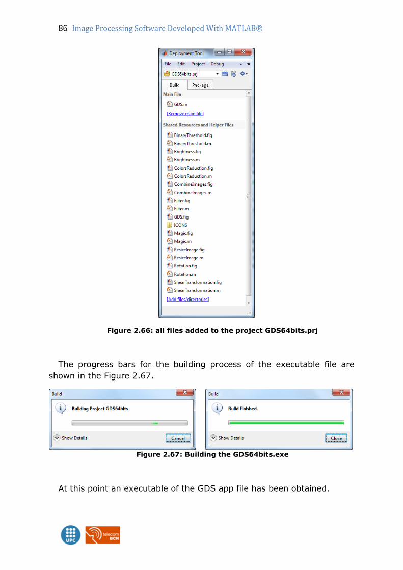
86 Image Processing Software Developed With MATLAB®
Figure 2.66: all files added to the project GDS64bits.prj
The progress bars for the building process of the executable file are
shown in the Figure 2.67.
Figure 2.67: Building the GDS64bits.exe
At this point an executable of the GDS app file has been obtained.
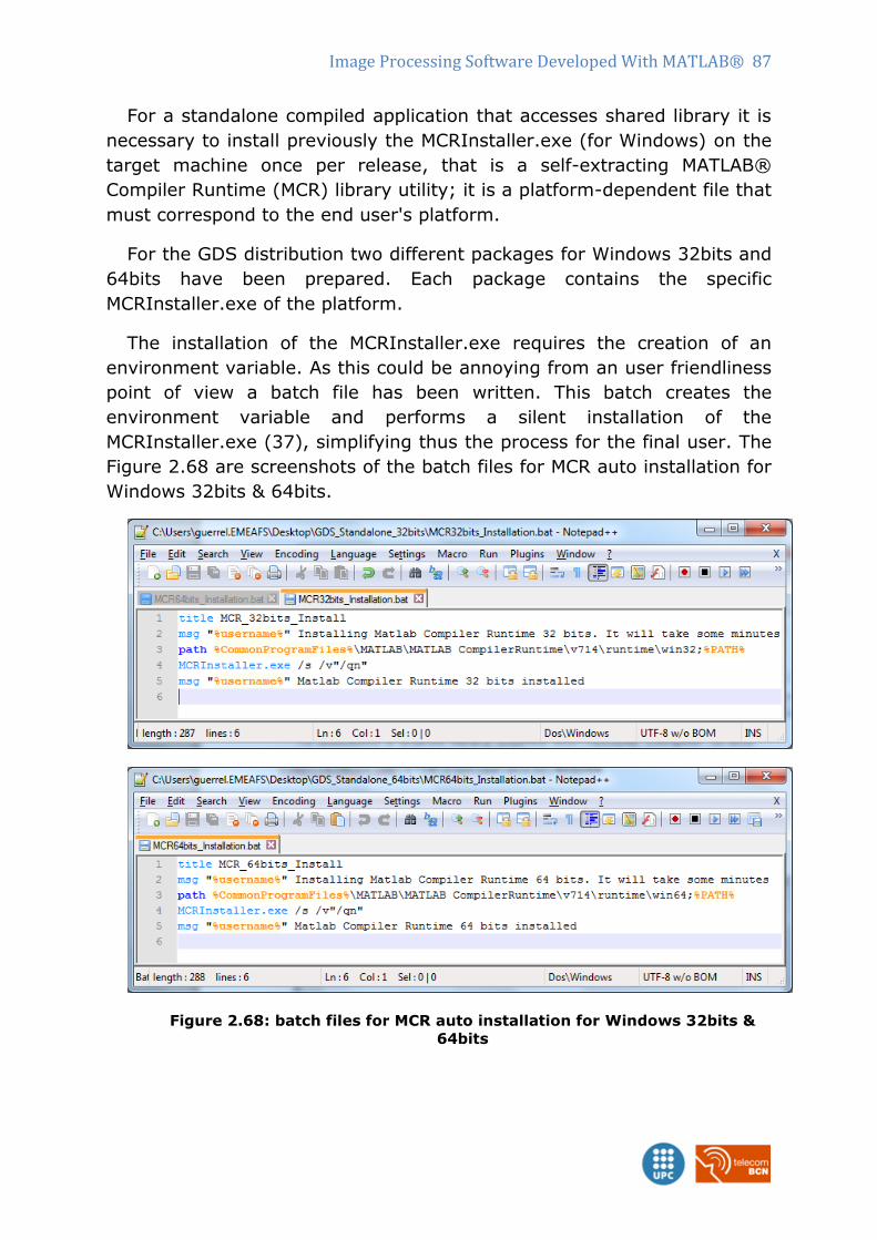
Image Processing Software Developed With MATLAB® 87
For a standalone compiled application that accesses shared library it is
necessary to install previously the MCRInstaller.exe (for Windows) on the
target machine once per release, that is a self-extracting MATLAB®
Compiler Runtime (MCR) library utility; it is a platform-dependent file that
must correspond to the end user's platform.
For the GDS distribution two different packages for Windows 32bits and
64bits have been prepared. Each package contains the specific
MCRInstaller.exe of the platform.
The installation of the MCRInstaller.exe requires the creation of an
environment variable. As this could be annoying from an user friendliness
point of view a batch file has been written. This batch creates the
environment variable and performs a silent installation of the
MCRInstaller.exe (37), simplifying thus the process for the final user. The
Figure 2.68 are screenshots of the batch files for MCR auto installation for
Windows 32bits & 64bits.
Figure 2.68: batch files for MCR auto installation for Windows 32bits &
64bits
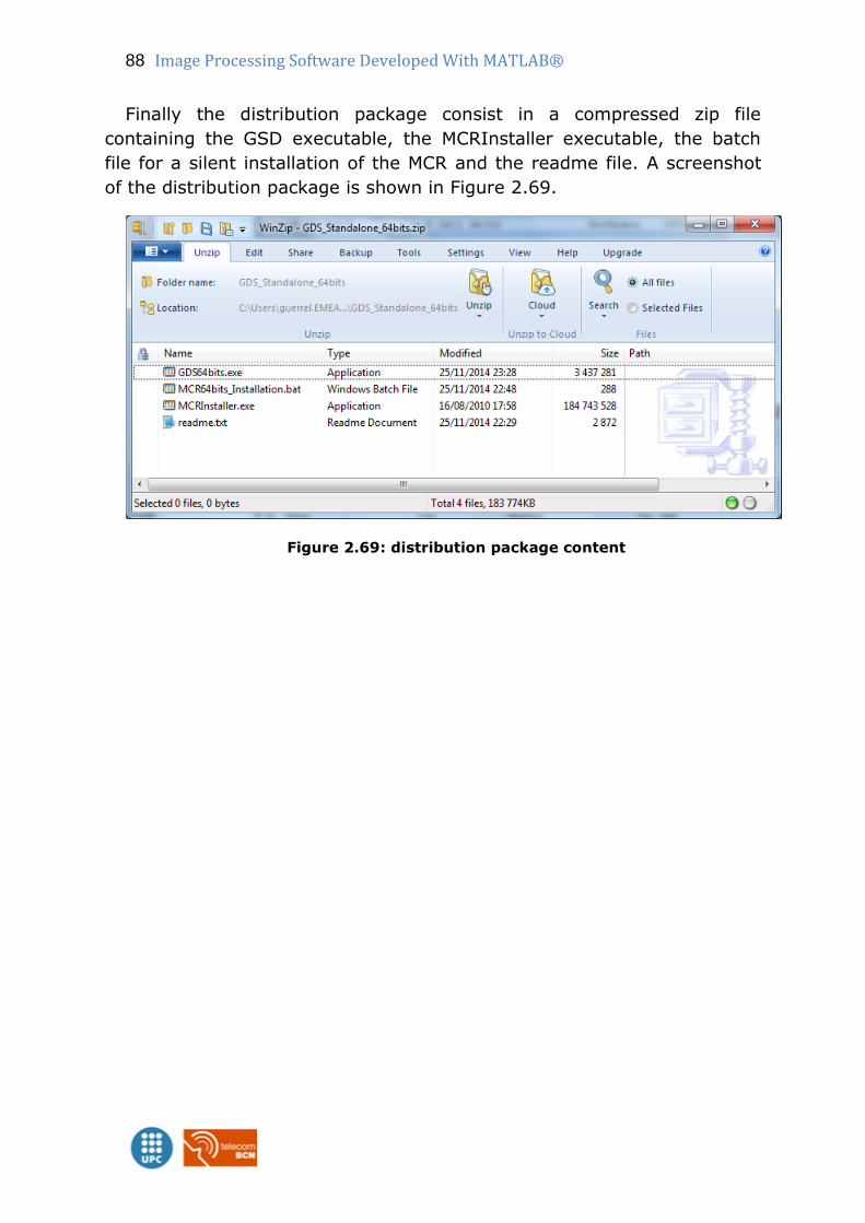
88 Image Processing Software Developed With MATLAB®
Finally the distribution package consist in a compressed zip file
containing the GSD executable, the MCRInstaller executable, the batch
file for a silent installation of the MCR and the readme file. A screenshot
of the distribution package is shown in Figure 2.69.
Figure 2.69: distribution package content
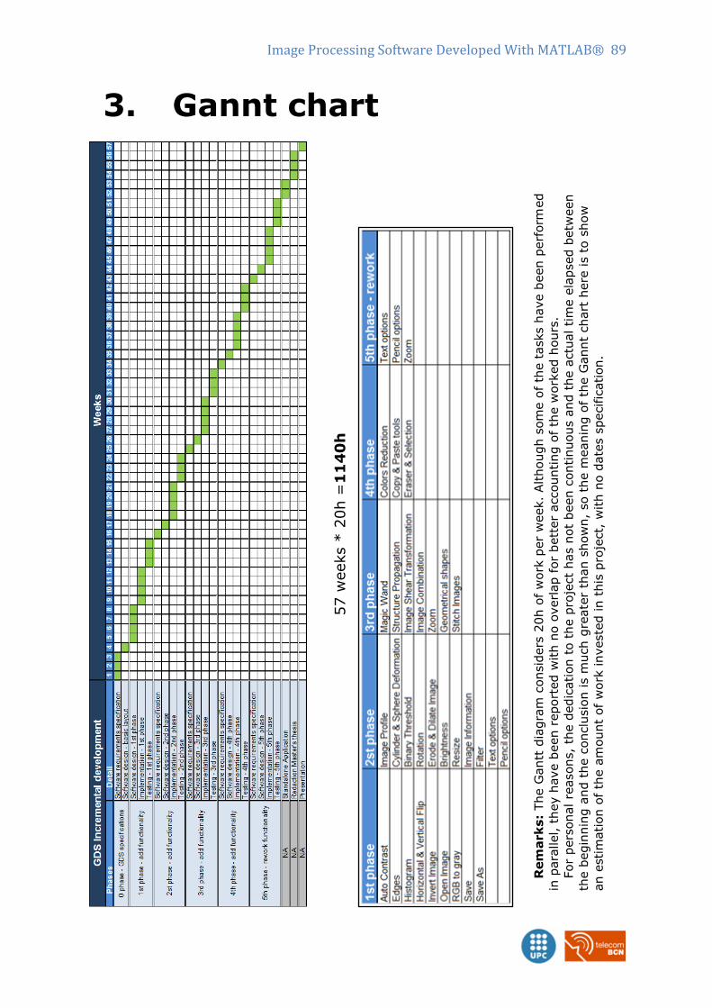
Image Processing Software Developed With MATLAB® 89
3. Gannt chart
57 w
eeks *
20h =
11
40
h
R
em
ark
s:
The G
antt
dia
gra
m c
onsid
ers
20h o
f w
ork
per
week.
Although s
om
e o
f th
e t
asks h
ave b
een p
erf
orm
ed
in p
ara
llel, t
hey h
ave b
een r
eport
ed w
ith n
o o
verlap f
or
bett
er
accounting o
f th
e w
ork
ed h
ours
.
F
or
pers
onal re
asons,
the d
edic
ation t
o t
he p
roje
ct
has n
ot
been c
ontinuous a
nd t
he a
ctu
al tim
e e
lapsed b
etw
een
the b
egin
nin
g a
nd t
he c
onclu
sio
n is m
uch g
reate
r th
an s
how
n,
so t
he m
eanin
g o
f th
e G
annt
chart
here
is t
o s
how
an e
stim
ation o
f th
e a
mount
of
work
investe
d in t
his
pro
ject,
with n
o d
ate
s s
pecific
ation.
90 Image Processing Software Developed With MATLAB®
4. Conclusions
Regarding the strong points of the project itself, the most remarkable
of all would be that the GDS has turned out to be a fully functional tool. I
have found myself using it for personal and professional reasons as it is in
many aspects more useful and easier to use than other professional
software solutions so I am in position to say that not only I am satisfied
with the program as a developer, but also as an amateur user.
The successful creation of the Standalone Package (also including the
silent installation of the MATLAB® Compiler Runtime library utility) is
another good point. See section 2.5 Standalone Application. The software
has been installed in several Operative Systems from Windows (Windows
XP 32 bits, Windows 7 32 bits, Windows 7 64 bits, Windows 8.1 64 bits)
and different computers with no issues found. Thus the GDS has been
easily distributed to several users, although no MATLAB® version was
installed on the target PC.
Another aspect worthy to bring forward would be the robustness of the
code. I have worked as a test engineer for several years in different
industries and I think that my project has strongly benefited from this
professional background. Many hours have been consecrated to properly
and thoroughly debugging the code to the slightest details. I am
particularly proud of this task, that at an industrial level would have
required several weeks of alpha and beta testing, and I believe that the
result exceeds the expectations that one could have for a one man job.
The tools required as objectives for the project have been
implemented, all of them included in section 2.3.1 Toolbar:
User interface for using Filters.
ROI Based Processing. Check in section 2.3.1 Toolbar/ Magic
Wand, Eraser & Selection.
Stitch Images.
Combine images.
Shear Transformation.
Structure Propagation.
Copy & Paste tools.
Regarding the possibilities for further development of the tool, several
aspects could be of interest: the first of all would be adding even more
features to the software; in the graphic industry, the possibilities are
Image Processing Software Developed With MATLAB® 91
virtually endless and one can always think of new automated functions
that could be of interest to some particular users depending on the
specialized use they would like to make of the tool.
Another point, of course, would be further debugging of the minor
inconveniences that might still be found while using the GDS. Proper
debugging of a code is a never-ending task and, should its capabilities be
enhanced, a new global system test should be performed.
Another interesting point to be developed would be the use of MATLAB
Mobile™ to run a simplified version of the GDS with Android. The MATLAB
Mobile™ is an application that allows remote connection from an Android
smartphone or tablet to a MATLAB® session running on MathWorks®
Cloud or on a computer.
Finally, from a personal perspective, this project has allowed me to
reach one of the most important objectives that I was pursuing when I
initially chose the subject: Improve my programming skills. Facing the
typical software issues such as designing the program, debugging,
validating, structuring the user interface, choosing the tools behavior and
so on, I had the chance to enhance my capabilities.
In this particular project I have improved my understanding of the tool
in general and of its data processing in particular. Many of the functions
used in this project can be used in environments other than the image
processing, and I expect that the knowledge that I have acquired will be
of great use for me in my professional career.
I believe that it is necessary for any engineer today to be able to
program his own tools and I am confident than I am now much more
performing in this aspect than I was before.
To sum up, this project has allowed me to reach the main objectives we
set out for at the beginning: improve my programming knowledge, and
create a high performing MATLAB® based image processing application.
92 Image Processing Software Developed With MATLAB®
5. Annexes
The annexes of the master's thesis: Image Processing Software
developed with MATLAB® (Graphic Design Software - GDS) have been
compiled together in the Annexes booklet.
Image Processing Software Developed With MATLAB® 93
6. References
1. Discovery/ MATLAB GUI. MathWorks website. [En línia] MathWorks®.
http://www.mathworks.com/discovery/matlab-gui.html.
2. Garrison, David. Writing Apps in MATLAB - Newsletter. MathWorks website.
[En línia] MathWorks®, 2012.
http://www.mathworks.com/company/newsletters/articles/writing-apps-in-
matlab.html?s_tid=mlg_b_appswr.
3. MATLAB CENTRAL/ File Exchange. MathWorks website. [En línia]
MathWorks®.
http://www.mathworks.com/matlabcentral/fileexchange/?s_tid=gn_mlc_fx.
4. MATLAB/ GUI Building/ GUI Building Basics/ Files Generated by GUIDE.
MathWorks website. [En línia] MathWorks®.
http://es.mathworks.com/help/matlab/creating_guis/files-generated-by-guide.html.
5. MATLAB/ Data Import and Export/ Standard File Formats/ Images/ imfinfo.
MathWorks website. [En línia] MathWorks®.
http://es.mathworks.com/help/matlab/ref/imfinfo.html?searchHighlight=imfinfo.
6. MATLAB/ Graphics/ Images/ Modifying Images/ rgb2gray. MathWorks website.
[En línia] MathWorks®.
http://es.mathworks.com/help/matlab/ref/rgb2gray.html?searchHighlight=rgb2gray.
7. Image Processing Toolbox/ Image Enhancement/ Morphological Operations/
imerode. MathWorks website. [En línia] MathWorks®.
http://es.mathworks.com/help/images/ref/imerode.html.
8. Image Processing Toolbox/ Image Enhancement/ Morphological Operations/
imdilate. MathWorks website. [En línia] MathWorks®.
http://es.mathworks.com/help/images/ref/imdilate.html.
9. MATLAB/ Language Fundamentals/ Matrices and Arrays/ Sorting and
Reshaping Arrays/ flipdim. MathWorks website. [En línia] MathWorks®.
http://es.mathworks.com/help/matlab/ref/flipdim.html.
10. MATLAB/ Graphics/ 2-D and 3-D Plots/ Surfaces, Volumes, and Polygons/
Surface and Mesh Plots/ cylinder. MathWorks website. [En línia] MathWorks®.
http://es.mathworks.com/help/matlab/ref/cylinder.html.
11. MATLAB/ Graphics/ 2-D and 3-D Plots/ Surfaces, Volumes, and Polygons/
Surface and Mesh Plots/ sphere. MathWorks website. [En línia] MathWorks®.
http://es.mathworks.com/help/matlab/ref/sphere.html.
94 Image Processing Software Developed With MATLAB®
12. Image Processing Toolbox/ Image Analysis/ Region and Image Properties/
improfile. MathWorks website. [En línia] MathWorks®.
http://es.mathworks.com/help/images/ref/improfile.html.
13. Image Processing Toolbox/ Image Analysis/ Region and Image Properties/
imhist. MathWorks website. [En línia] MathWorks®.
http://es.mathworks.com/help/images/ref/imhist.html.
14. Image Processing Toolbox/ Geometric Transformations, Spacial Referencing
and Image Registration/ Geometric Transformations/ maketform. MathWorks
website. [En línia] MathWorks®.
15. Image Processing Toolbox/ Geometric Transformations, Spacial Referencing
and Image Registration/ Geometric Transformations/ imtransform. MathWorks
website. [En línia] MathWorks®.
http://es.mathworks.com/help/images/ref/imtransform.html.
16. Image Processing Toolbox/ Geometric Transformation, Spatial Referencing,
and Image Registration/ Geometric Transformations/ imresize. MathWorks website.
[En línia] MathWorks®. http://es.mathworks.com/help/images/ref/imresize.html.
17. Image Processing Toolbox/ Display and Exploration/ Build Interactive Tools/
imcrop. MatWorks website . [En línia] MatWorks® .
http://es.mathworks.com/help/images/ref/imcrop.html.
18. Image Processing Toolbox/ Display and Exploration/ Build Interactive Tools/
imline. MatWorks website. [En línia] MatWorks®.
http://es.mathworks.com/help/images/ref/imline.html.
19. Giusti, Alessandro. To stitch two images. Leet. [En línia]
http://www.leet.it/home/giusti/teaching/matlab_sessions/stitching/stitch.html.
20. Image Processing Toolbox/ Image Analysis/ Object Analysis/ edge.
MathWorks website. [En línia] MathWorks®.
http://es.mathworks.com/help/images/ref/edge.html.
21. Canny, John. "A Computational Approach to Edge Detection, IEEE
Transactions on Pattern Analysis and Machine Intelligence". 1986.
22. MATLAB/ Graphics/ Images/ Modifying Images/ rgb2ind. MathWorks website.
[En línia] MathWorks®. http://es.mathworks.com/help/matlab/ref/rgb2ind.html.
23. Image Processing/ Toolbox& Image Enhancement/ Image Filtering.
MathWorks website . [En línia] MathWorks®.
http://es.mathworks.com/help/images/ref/fspecial.html.

Image Processing Software Developed With MATLAB® 95
24. Image Processing Toolbox/ Image Enhancement/ Image Filtering/ imfilter.
MathWorks website. [En línia] MathWorks®.
http://es.mathworks.com/help/images/ref/imfilter.html.
25. Image Processing Toolbox/ Image Enhancement/ Image Filtering/ medfilt2.
MathWorks website. [En línia] MathWorks®.
http://es.mathworks.com/help/images/ref/medfilt2.html#bupa1jh-1.
26. Image Processing Toolbox/ Image Enhancement/ Image Filtering/ wiener2.
MathWorks website. [En línia] MathWorks®.
http://es.mathworks.com/help/images/ref/wiener2.html?searchHighlight=wiener2.
27. Image Processing Toolbox/ Image Enhancement/ ROI-Based Processing/
roifill. MathWorks website. [En línia] MathWorks®.
http://es.mathworks.com/help/images/ref/roifill.html.
28. Image Processing Toolbox/ GPU computing/ bwlabel. MathWorks website. [En
línia] MathWorks®. http://es.mathworks.com/help/images/ref/bwlabel.html.
29. Tal, Yoram. MATLAB CENTRAL/ File Exchange/ MagicWand2. MathWorks
website. [En línia] MathWorks®, 2004.
http://www.mathworks.com/matlabcentral/fileexchange/6034-
magicwand2/content/magicwand2.m.
30. Image Processing Toolbox/ Display and Exploration/ Build Interactive Tools/
imfreehand. MathWorks website. [En línia] MathWorks®.
http://es.mathworks.com/help/images/ref/imfreehand.html.
31. MATLAB/ Graphics/ Images/ Modifying Images/ ind2rgb. MathWorks website.
[En línia] MathWorks®. http://es.mathworks.com/help/matlab/ref/ind2rgb.html.
32. Image Processing Toolbox/ Image Analysis/ Region and Image Properties/
impixel. MathWorks website. [En línia] MathWorks®.
http://es.mathworks.com/help/images/ref/impixel.html.
33. Figure Properties. MathWorks® website. [En línia] MathWorks®.
http://es.mathworks.com/help/matlab/ref/figure-properties.html.
34. MATLAB/ Graphics/ Formatting and Annotation/ Data Exploration/ zoom.
MathWorks website. [En línia] MathWorks®.
http://es.mathworks.com/help/matlab/ref/zoom.html.
35. MATLAB/ Graphics/ Images/ Image File Operations/ imwrite. MathWorks
website. [En línia] MathWorks®.
http://es.mathworks.com/help/matlab/ref/imwrite.html.
96 Image Processing Software Developed With MATLAB®
36. Image Processing Toolbox/ Display and Exploration/ Build Interactive Tools/
imsave. MathWorks website. [En línia] MathWorks®.
http://es.mathworks.com/help/images/ref/imsave.html?searchHighlight=imsave.
37. Matlab Answers : How do I silently install the MATLAB Compiler Runtime
(MCR)? MathWorks website. [En línia] Mathworks®.
http://www.mathworks.com/matlabcentral/answers/106020-how-do-i-silently-install-
the-matlab-compiler-runtime-mcr.