Master's thesis first page med blanksida - Lund University...
94
Master’s Thesis Dynamic effects generated by trains on railway bridges Enrico Pasqualetti Rylander _________________________________________________ Department of structural engineering Lund University of Technology Lund University, 2006 Report TVBK – 5145
Transcript of Master's thesis first page med blanksida - Lund University...
Master’s Thesis
Dynamic effects generated by trains on railway bridges
Enrico Pasqualetti Rylander _________________________________________________ Department of structural engineering Lund University of Technology Lund University, 2006
Report TVBK – 5145


I
Lund University of Technology Department of Structural Engineering Box 118 S-221 00 Lund Sweden
DYNAMIC EFFECTS GENERATED
BY TRAINS ON RAILWAY BRIDGES
Dynamiska effekter genererade av trafiklaster i järnvägsbroar
Enrico Pasqualetti Rylander, Lund 2006
Abstract Sustainable Bridges is an EU-project. The objective of the project is to demonstrate that it is possible to enhance the load capacity of a bridge with refined analytical methods. This thesis will be a small part of the project. My objective in this thesis is to examine the dynamic loads generated in a bridge when trafficked. Since there are uncertainties concerning the dynamic effect this variable should be considered stochastic. Previous research confirms that the size of this variable is dependent on the force, the bending stiffness, the damping, the frequency and the velocity among others. In reliability analysis of a bridge there is a need of statistical information. This information is scarce for dynamic effects, therefore it will be examined.

II
Report TVBK-5145 ISSN: 0349-4969 ISRN: LUTVDG/TVBK-06/5145+92p Thesis Supervisor: Senior researcher Fredrik Carlsson Examiner: Professor Sven Thelandersson November, 2006

III
ACKNOWLEDGEMENT
This thesis has become a reality with the excellent help of my supervisor, senior researcher Mr. Fredrik Carlsson. From start to finish he has been there to support and guide me. I would also like to thank Professor Mr. Sven Thelandersson for his advice and contributions. A special dedication goes to my grandfather Uno Rylander, who has always been my inspiration and of course to my sunshine Lejla Šehović.
IV
ABSTRACT
The concept of dynamic effects imposed by train loads on bridges is a scarcely researched area, compared to the effects imposed by the static loads. The comprehension of dynamic behavior is therefore limited. Today it is common to add the dynamic loads to the static load using a very general multiplication factor. This conservative method of treating dynamic effects in the codes is in general not economically justified since the bridge elements become unnecessarily large. To improve the understanding of dynamic load effects a theoretical study is conducted, where several variables are taken under consideration to evaluate which of these are the important ones. The base to determine these important parameters is a standard bridge taken from the SRA. This bridge is a simply supported concrete bridge with a span of 10 meters. Values for static bending moment and dynamic bending moment are calculated and the dynamic amplification factors are determined. A statistical study is made to examine the variation of the dynamic amplification factor by simulating several trains traversing the same bridge. In this study the parameters are treated as random variables to make the analysis realistic and exclude any uncertainties. When satisfactory results are achieved, statistical distributions of the dynamic amplification are determined and presented in a table for different spans and velocities.

V
Short summary
The thesis consists of:
1. Introduction – description of the area of research. The origins and the benefits of the analysis are put forward, with the objective and restrictions of this thesis.
2. State of the art – contains today’s coverage of dynamic factors and loads in different codes. Describes how the dynamic amplification factor is represented in the different codes and gives an account of the dynamic loads. The main objective is to extract important details from the codes and shed light on the important content for this case.
3. Analytical model – contains the analytical model to determine dynamic amplification factors, static and dynamic moment and a description of the correspondent Matlab code.
4. Parametric study – the influence of the dynamic effect for different parameters is investigated. The studied parameters are axle loads, train velocity, bending stiffness, frequency and damping of the bridge. Several dynamic amplification factors, dynamic and static moment are presented for the different parameters.
5. Statistical evaluation – contains statistical distributions for the dynamic amplification factor, which are determined by simulations. The Monte Carlo simulation is performed to evaluate the statistical dynamic amplification factors that encompass all the important parameters.
6. Dynamic amplification factors – consists of the dynamic factors, collected to give an overview of the results in the form of a table. A discussion concerning the results is provided.

VI
LIST OF ABBREVIATIONS
BV BRO BV Bro 2004, release 7 (utgåva 7), Swedish bridge design
code, (Banverkets ändringar och tillägg till vägverkets Bro
2004)
EC1 Eurocode 1: Actions on structures, Traffic load on bridges,
European standard 2002
SRA Swedish rail road administration, (Banverket)
HSML Theoretical dynamic train load
MSE Mean square distance from diagonal line in the quantile plot,
(Eq. 5.6)
LIST OF SYMBOLS
Chapter 1
TS Total traffic load
SS Static load
DS Dynamic load
.ε Dynamic amplification factor
Chapter 2
φ Dynamic amplification factor, EC1
φL Determinant length associated with φ
D Dynamic amplification factor, BV BRO
bestL Determinant length
d∆ Coefficient for reducing the dynamic amplification factor
designv Design speed
maxv Maximum allowable speed

VII
Chapter 3
F Force t Time f First natural frequency
l Span length c Train velocity EI Bending stiffness ν Damping h Axle coefficient j Mode
x Distance
nt Time when the thn axle starts traversing the bridge
nT Time when the thn axle finishes traversing the bridge
M Bending moment d Distance between axle loads ω Excitation frequency
Chapter 4
DAF Dynamic amplification factor Md Dynamic bending moment Ms Static bending moment
Chapter 5
F Cumulative distribution function
F̂ Empirical distribution function n Number of simulations

VIII

IX
TABLE OF CONTENT
1 INTRODUCTION_____________________________________________1
1.1 Background____________________________________________________________ 1 1.2 Objectives _____________________________________________________________ 2 1.3 Limitations ____________________________________________________________ 3
2 STATE OF THE ART, DYNAMIC FACTORS______________________5
2.1 EC1 __________________________________________________________________ 5 2.1.1 Definition and application of dynamic factors .φ _______________________5 2.1.2 Limitations ____________________________________________________6 2.1.3 Dynamic analysis _______________________________________________7 2.1.4 Definition of dynamic loads _______________________________________7 2.1.5 Application of dynamic loads______________________________________8 2.1.6 Train type A6, EC1______________________________________________9
2.2 BV Bro_______________________________________________________________ 10 2.2.1 Definition and application of the dynamic factor______________________10 2.2.2 Limitations ___________________________________________________10 2.2.3 Dynamic loads ________________________________________________11
2.3 Conclusions ___________________________________________________________ 12
3 ANALYTICAL MODEL _______________________________________13
3.1 Introduction __________________________________________________________ 13 3.2 Frýba model __________________________________________________________ 13
3.2.1 Description of the parameters involved in the Frýba model______________14 3.3 Matlab code___________________________________________________________ 17
3.3.1 Converting into Matlab language __________________________________17 3.3.2 Definition and application of the parameters _________________________17
4 PARAMETRIC STUDY _______________________________________21
4.1 General ______________________________________________________________ 21 4.2 Force ________________________________________________________________ 24 4.3 Velocity ______________________________________________________________ 25 4.4 Bending stiffness _______________________________________________________ 27 4.5 Frequency ____________________________________________________________ 28 4.6 Damping _____________________________________________________________ 29 4.7 Conclusions ___________________________________________________________ 31
5 STATISTICAL EVALUATION _________________________________33
5.1 Introduction __________________________________________________________ 33 5.2 Monte Carlo simulation _________________________________________________ 33

X
5.3 Statistical parameter composition_________________________________________ 33 5.4 Goodness of fit ________________________________________________________ 35
6 DYNAMIC AMPLIFICATION FACTORS________________________37
6.1 Introduction __________________________________________________________ 37 6.2 Final results___________________________________________________________ 39 6.3 Conclusions ___________________________________________________________ 40
REFERENCES _______________________________________________42
APPENDIX __________________________________________________44
A Matlab Code ___________________________________________________________ 45 B Figures Matlab _________________________________________________________ 49 C Monte Carlo simulation __________________________________________________ 51 D Figures Monte Carlo ____________________________________________________ 55
D.1 Bridge span of 5 meters, velocity of 150 km/h, standard deviation of 22,5 km/h ____ 55 D.2 Bridge span of 5 meters, velocity of 200 km/h, standard deviation of 30 km/h ______ 58 D.3 Bridge span of 5 meters, velocity of 250 km/h, standard deviation of 37,5 km/h ____ 60 D.4 Bridge span of 10 meters, velocity of 150 km/h, standard deviation of 22,5 km/h ___ 62 D.5 Bridge span of 10 meters, velocity of 200 km/h, standard deviation of 30 km/h _____ 65 D.6 Bridge span of 10 meters, velocity of 250 km/h, standard deviation of 37,5 km/h ___ 67 D.7 Bridge span of 15 meters, velocity of 150 km/h, standard deviation of 22,5 km/h ___ 69 D.8 Bridge span of 15 meters, velocity of 200 km/h, standard deviation of 22,5 km/h ___ 72 D.9 Bridge span of 15 meters, velocity of 250 km/h, standard deviation of 37,5 km/h ___ 74 D.10 Bridge span of 20 meters, velocity of 150 km/h, standard deviation of 22,5 km/h __ 76 D.11 Bridge span of 20 meters, velocity of 200 km/h, standard deviation of 30 km/h ____ 79 D.12 Bridge span of 20 meters, velocity of 250 km/h, standard deviation of 37,5 km/h __ 81

1
1 Introduction
1.1 Background Times are constantly changing. Trains are getting larger, ergo heavier. Since people always are in a hurry and trains want to compete with airplanes, trains are also getting faster. How does this affect existing European railway bridges? The increasing need to upgrade bridges in Europe brings us to the main area of study for this thesis. The dynamic effects imposed on bridges due to increased velocity and weight are examined.
The economical benefit of improving values of dynamic effects is significant, because this will optimize the bridge design compared to the conservative dynamic amplification values currently used. This optimization will be beneficial for new bridges as well as for maintenance and upgrading of existing bridges.
In this thesis, focus will be kept on the dynamic part of the traffic load. Parameters with significant importance when dealing with dynamic behavior are:
• the bridge damping • the train velocity • the mass of the structure • the span length • the number of axles • distance between the axles • the axle loads • the construction materials behavior • the dynamic properties of the train and of the track • the suspension characteristics • the unsprung/sprung mass of the train • vertical irregularities in the track • the natural frequencies of the whole structure • relevant elements with associated eigenmodes
The most dominating variable load on railway bridges is the load generated by trains. The traffic load imposed on a bridge consists of two parts, one part from the static load and the other from the dynamic load. Static loads are generated in the bridge from the weight of the train and placing of the point
2
loads from the axles. Dynamic loads are generated in the bridge because the train is brought into vertical sway.
The total traffic load TS is composed of the static load SS and the dynamic
load DS
DST SSS += Eq. 1.1
It is very common in different codes that the dynamic load is replaced by a dynamic amplification factor, .ε
ε⋅=
+⋅=+= S
S
D
SDST SS
SSSSS 1 Eq. 1.2
The dynamic amplification factors described today in different codes are very general and therefore conservative since they have to be applicable on different bridge systems. The dynamic part could in some cases be as much as 50 % of the total traffic load (EC1 2002). This implies that dynamic loads have a large influence in the design of a new bridge or when examining the safety level of existing bridges. Therefore it is of great importance to get a wider knowledge of the dynamic amplification factor, which is exactly the purpose of this study.
1.2 Objectives How are the dynamic effects described in the different codes, and can they be improved to give a more precise value of the dynamic effects in specific cases? The traffic load from a train is the most important variable load imposed on a bridge (SRA). In current standards the dynamic amplification factor is between 1.00 and 2.00, ergo it is of great importance. In a probability based analysis there is a need for information about the statistical distribution of the factor. The statistical distribution of the dynamic amplification factor will be the final result of this thesis.

3
1.3 Limitations The thesis will contain a study of the dynamic effects on simply supported bridges with shorter spans. The main construction material under observation will be reinforced concrete. In this thesis the area of focus will be kept to European railway bridges. The main literature will be EC1 2002 and BV BRO 2004 and dynamic loads according to these codes will be used for the study.
The parameters studied will be limited to:
• axle force
• train velocity
• bending stiffness
• frequency
• damping

4
5
2 State of the art, dynamic factors
2.1 EC1
2.1.1 Definition and application of dynamic factors .φ
The dynamic factors are specified as 2φ or 3φ . 2φ is the dynamic amplification
factor used for carefully maintained tracks as seen in equation 2.1 and 3φ is the
dynamic amplification factor used for tracks with standard maintenance according to equation 2.2. The factors take into account the dynamic magnification of stresses and vibration effects but do not take resonance effects into account.
In the quasi static method used to determine dynamic effects, the static load is multiplied by a deterministic dynamic factorφ . To take into account
resonance effects a dynamic analysis is required.
The dynamic factors 2φ and 3φ are determined depending on the
condition of the track. For carefully maintained tracks the maximum value of the dynamic factor is 67,12 =φ which is smaller than the value for tracks with
standard maintenance, where 00,23 ≤φ . φL is the determinant length1 in
meters, associated with .φ Table 6.2 in EC1 – Part 2: Traffic load on structures,
pages 79 – 81, describes how to evaluate the correct determinant length for different bridge constructions. Carefully maintained tracks:
82,02,0
44,12 +
−=
φ
φL
Eq. 2.1
Tracks with standard maintenance:
73,02,0
16,23 +
−=
φ
φL
Eq. 2.2
1 Determinant length for the simply supported bridge considered in this thesis is the span
6
2.1.2 Limitations
In EC1, the dynamic factors were established for simply supported girders, since this construction is the easiest to analyze. If no dynamic factor is established because of difficulties in deciding the condition of the tracks, 3φ
will be used, which is the most conservative factor. In the case of arch bridges and concrete bridges with a cover2 of mh 00,1> , the dynamic factor may be reduced to:
00,110
00,13,23,2 ≥
−−=
hred φφ Eq. 2.3
In this value of dynamic amplification factors, impact and resonance effects are not taken into account. Excessive vibration of the bridge could lead to ballast instability, excessive deflection and stresses. To take into account these unwanted effects a dynamic analysis is required. The dynamic factor shall not be used with the loading due to Real Trains, (which are also theoretical trains described in EC1), the loading due to Fatigue Trains, load Model HSLM or the load model unloaded train (EC1 2002).
2 The cover is the thickness of the overlaying ballast on the bridge

7
2.1.3 Dynamic analysis
A dynamic analysis is required according to the flow chart in Figure 2.1 taken from EC1 – Part 2: Traffic load on structures, page 75, Figure 6.9. Some of the involved parameters are the train speed, type of construction, span length, eigenforms and frequency. From Figure 2.1 it is obvious that for train speeds less than 200 km/h on continuous bridges, a dynamic analysis is not required. For some simple constructions a dynamic analysis could be required, depending on the natural frequency. Exceeding the speed of 200 km/h on continuous bridges immediately requires a dynamic analysis. For some simple constructions a dynamic analysis is required depending on the span length and the natural frequency of the bridge. Figure 2.1 Flow chart for determining whether
a dynamic analysis is required (EC1, 2002)
2.1.4 Definition of dynamic loads
A dynamic analysis is performed using characteristic values of the loading from Real Trains specified for every particular project. Load Model 71, SW/0 for continuous bridges and SW/2 for heavy loads are all static loads. The load model “unloaded train” represents the effect of an unloaded train which consists of vertical uniformly distributed load with a characteristic value of 10 kN/m.
The dynamic load model HSML represents trains that exceed 200 km/h (124.3 miles/h) which consists of two separate universal trains with variable

8
coach lengths, HSML-A and HSML-B. Together they represent the dynamic load effects of a single axle, an articulated axle and a conventional high speed passenger trains.
2.1.5 Application of dynamic loads
The area of application for the dynamic loads is shown in Table 2.1. Load case HSML-B is used for simply supported structures with a short span. It is constituted of any number of point loads of 170 kN with a specified distance in between.
Table 2.1 Application for dynamic loads, EC1
Span Structural configuration mL 7< mL 7≥
Simply supported span HSML-B HSML-A Continuous structure or Complex Structure
HSML-A Trains A1 to A10 inclusive
HSML-A Trains A1 to A10 inclusive
When designing a continuous or complex structure all the train load models A1 to A10 according to Table 2.2 should be used. For simply supported constructions with a span equal to or greater than 7 meters a single critical Universal Train from HSML-A (Train load model A1 to A10) can be used. To achieve a more complete dynamic analysis all the train load models could be used. If the leading and trailing power cars are not identical on a train then a consultation must be made with the National Annex of the European standard.

9
Table 2.2 Train load models, EC1
Load Model
Number of wagons in between
Length of wagons (m)
Wheel spacing between boogie (m)
Axle load (kN)
A1 18 18 2,0 170 A2 17 19 3,5 200 A3 16 20 2,0 180 A4 15 21 3,0 190 A5 14 22 2,0 170 A6 13 23 2,0 180 A7 13 24 2,0 190 A8 12 25 2,5 190 A9 11 26 2,0 210 A10 11 27 2,0 210 For passenger trains the maximum allowable speed of 350 km/h (217,5 miles/h) is used, to make a valid assessment of the dynamic effects. The maximum design speed shall be multiplied by 1.2 with the maximum line speed at the site.
2,1max ⋅= vvdesign Eq. 2.4
2.1.6 Train type A6, EC1
Figure 2.2 represents the train model A6. This train model is the one that will be used in this research. Every wheel on the train is seen as a point load F of 180 kN. D is the coach length and d is the wheel spacing within a boogie.
Figure 2.2 Train type A6, according to EC1
d D
d d
D
F
ln
n
Direction of the train
1 2
10
2.2 BV Bro
2.2.1 Definition and application of the dynamic factor
The first thing that is obvious to the reader is that looking for a specific chapter after dynamic action is meaningless. The dynamic influence is integrated in the Swedish standard as a deterministic dynamic amplification factor, D . The dynamic amplification factor is to be integrated into the vertical load acting on the foundation and the bridge, given by:
bestLD
++=
8
400,1 Eq. 2.5
where bestL is the determinant length3 in meters, always larger than 2 meters,
which is the minimum span for a bridge to be classified as a bridge (SRA).
bestL is described in two different tables in BV BRO, one table for support on
both ends Table BV 21.2216a, page 40 and one for brackets Table BV 21.2216b, on page 41.
2.2.2 Limitations
The dynamic influence is not considered when/if it gives a favorable effect. The dynamic influence should not be considered in calculations concerning impact on the ground, on pile groups consisting of more than 4 piles and for deformation. All horizontal forces (breaking and acceleration force, wind load, centrifugal force and friction force) acting on the bridge deck are not to be increased with the dynamic multiplication factor. For bridges that are planned to support trains with speeds over 200 km/h (124,3 miles/h) a special investigation of the dynamical behavior of the bridge is necessary according to BV BRO, Appendix BV 2-2, pages 60-66. In the case of bridges with a cover4
mh 20,1> , the dynamic factor may be
reduced by:
( )20,110,0 −⋅=∆ hd Eq. 2.6
It results in a reduced dynamic amplification factor 00,1≥D .
00,1≥∆− dD Eq. 2.7
3 Determinant length for the simply supported bridge considered in this thesis is the span 4 The cover is the thickness of the overlaying ballast on the bridge

11
A special load case for the Swedish code is for a railway track changing machine with the load of 900 kN equally distributed on two surfaces where a dynamic multiplication factor of 1,20 is applicable.
2.2.3 Dynamic loads
Dynamic loads come into focus when a dynamic analysis is required, i.e. when train speeds exceed 200 km/h (124.3 miles/h). The dynamic loads HSML-A and HSML-B represent axle loads, trains with a common boogie and conventional high speed trains. HSLM-A shall be used for all bridges with train load models A1-A10, according to Table 2.2. HSML-B is used for simply supported bridges with a span less than 7 meters. HSML-B is constituted of any number of point loads of 170 kN with a specified wheel spacing between boogie. A dynamic analysis is performed for the interval of 100 km/h (62.1 miles/h) to the maximum line speed at the site plus 20%.
2,12,0 maxmaxmax ⋅=⋅+= vvvvdesign Eq. 2.8

12
2.3 Conclusions The area of focus is Europe and especially Sweden where the study is conducted. It is obvious that the span length is of great importance when dealing with static moments as well as dynamic moments. EC1 dated July 2002 takes the maintenance of the tracks into account which is not a parameter in the Swedish code, BV BRO dated first of October 2004. Resonance and impact effects are not accounted for in the different codes, only the dynamic magnification of stresses and vibrations imposed on a bridge. The Dynamic amplification factors used are deterministic. Similarities between the codes are that when trains exceed 200 km/h (124.3 miles/h) a dynamic analysis is required, but in the EC1 a dynamic analysis is applicable on continuous bridges and on some simple constructions depending on the span length and natural frequency. In the EC1 the maximum allowable vehicle speed is 350 km/h (217.5 miles/h), a limit that is not mentioned in the BV BRO. The BV BRO states that if the dynamic influence gives a favorable effect it should not be taken into account for horizontal or vertical forces. A reduced dynamic factor is used in the EC1 for arch or concrete bridges with a cover more than 1 meter, in the BV BRO for bridges with a cover greater than 1.20 meters. The BV BRO takes into account a special load case, which is the railway track changing machine with a dynamic amplification factor of 1.20, which is surplus information not mentioned in the EC1. The codes are similar but in some aspect they complete each other. The important thing to keep in mind when dealing with dynamic loads is to determine a determinant length, multiply the maximum line speed with 1.2, see equation 2.4 and 2.8, and use the right train load model.

13
3 Analytical Model
3.1 Introduction Chapter 3 describes the Frýba model, which is the foundation to determine dynamic amplification factors in this thesis. The parameters involved in the Frýba model (L. Frýba 2003) are described to give an understanding of the content in the model. The parameters are converted into Matlab language and then an explanation follows of the procedure in the Matlab programming code.
3.2 Frýba model To determine the total static and dynamic bending moment a model by Frýba is used. This equation has been the building stone of the analytical model which is built upon the famous Bernoulli-Euler differential equation with further development from the Fourier and Laplace-Carson transformations (L. Frýba 2003). The simply supported bridge is subjected to several moving point loads. To study the bending moment time histories the Frýba equation is used. For a simply supported bridge, the moment at location x at time t is given by:
( )( )
( ) ( ) ( ) ( ) ( )[ ]∑∑∞
= =
−−−−−−=∂
∂−=
1 1
21
302
2
sin1,
,j
N
n
nn
j
nn
n
l
xjTthTtftthttfj
F
FM
x
txEItxM
πωω
ν Eq. 3.1
where 0M is the static bending moment at location x and nF is the static axle
load of axle n according to Figure 3.1. N and j are the total number of axles
and modes respectively. nt and nT are the times when the number n axle
enters and leaves the bridge respectively.

14
Figure 3.1 Visual declaration of variables related to the Frýba model. l is the
span of the bridge and c is the velocity of the train (L. Frýba, 2003).
3.2.1 Description of the parameters involved in the Frýba model
A short description follows which clarifies the variables involved in the model by Frýba (L. Frýba, 2003). [ ]
[ ][ ]
[ ][ ]
[ ] span Mid 2Lx
thesisin this considered be willmodefirst only the Mode,1
loads axlebetween Distance
Velocity
lengthSpan
frequency naturalFirst
Time
1
⇒=
⇒=
⇒
⇒
⇒
⇒=
⇒
m
j
md
smc
ml
Hzff
st
0M is the initial mid span bending moment according to Frýba, given by:
[ ]kNmFlFl
M4
220 ≈=
π Eq. 3.2
In the special case when all axel loads are equal equation 3.3 is valid.
[ ] FFkNF
Fn
n =⇒= 1 Eq. 3.3
l ct
x
d2 dn
Fn F1 F2
15
Equation 3.4 describes the time nt when the thn axle load begins traversing
the bridge. A visual declaration of nl is presented in Figure 2.2.
[ ]sc
lt n
n = Eq. 3.4
Equation 3.5 describes the time nT when the thn axle load finishes traversing
the bridge. A visual declaration of nl is presented in Figure 2.2.
[ ]sc
llT n
n
+= Eq. 3.5
)(th is the Heaviside unit function given by:
01
00)(
≥
<=
tif
tifth Eq. 3.6
The excitation frequency ω , is given by:
[ ] [ ]Hzsl
c=
⋅= 1π
ω Eq. 3.7
where l is the span of the bridge and c is the velocity of the train. The natural
frequency of the bridge jω for mode j is given by:
[ ]Hzl
EIjj
µ
πω
⋅
⋅⋅=
4
44
Eq. 3.8
where EI is the bending stiffness for a constant cross section of the beam and µ is the constant mass per unit length of the beam.
The function ( )tf is given by:
( ) ( ) ( ) [ ]HzttjjD
tf j
tj
j
d
+⋅⋅++⋅⋅
⋅⋅=
⋅− γωλωω
ω
ω
ω '
'
'sinexpsin
1 Eq. 3.9
where dω is the circular frequency of damping, given by:
[ ]Hzfd νω ⋅= 1 Eq. 3.10
where ν is the logarithmic decrement of damping and 1f is the first natural
frequency.
16
j'ω is given by:
[ ]Hzdjj
22' ωωω += Eq. 3.11
D is given by:
( ) [ ]HzjjD dj
2222222 4 ωωωω ⋅+⋅−= Eq. 3.12
λ and γ are given by:
[ ]Hzj
j
j
d
222
2arctan
ωω
ωωλ
⋅−
⋅⋅⋅−= Eq. 3.13
and
[ ]Hzjjd
jd
222'2
'2arctan
ωωω
ωωγ
⋅+−
⋅⋅= Eq. 3.14
In this study the interesting load position on the beam is in the middle2
lx = .
Equation 3.1 can be rewritten as:
( ) ( ) ( ) ( ) ( ) ( )[ ]∑∑∞
= =
−−−−−−=1 1
2
1
3
21
2,
j
N
nnn
j
nn
n TthTtftthttfjlF
txM ωωπ
Eq. 3.15

17
3.3 Matlab code In order to study the important parameters influencing the dynamic effects in railway bridges, a code describing all the parameters is constructed in the software program Matlab. The Matlab code is constructed to understand and examine what happens when a train traverses a bridge. The written program determines the static and dynamic mid span moment as a function of time. Different types of dynamic amplification factors are also evaluated to give a wider perspective. This thesis consists of two parts. The first part is constituted of a parametric study with the purpose of determining parameters which have a large influence on dynamic effects. The second part is constituted of a statistical parameter composition. The purpose is to determine a statistical description for the dynamic amplification factors. The statistical variables are used in the Monte Carlo simulation which is a modification of the initial Matlab code. Once the basic code is constructed it is easy to change the parameters to evaluate the different results. The Matlab code is described in appendix A, accompanied by diagrams in appendix B. The Monte Carlo simulation is described in appendix C, accompanied by diagrams in appendix D.
3.3.1 Converting into Matlab language
Shown in Table 3.1 is the conversion of the equation symbols into Matlab code. Some of the variables are not available in the Matlab program so they had to be modified.
Table 3.1 Conversion table
ν v µ my ω w
dω wd
jω wj
'jω wjj
λ lambda γ gamma
3.3.2 Definition and application of the parameters
This section describes the Matlab code shown in appendix A with related figures in appendix B. The results of running this program is the dynamic and
18
static mid span moment in a simply supported bridge generated by train model A6 as a function of time. The program also calculates different types of dynamic amplification factors which will be accounted for further on. General A security measure is imposed to close and clear all preceding information that the program may have saved. Results are delivered with proximity of four decimals. The semicolon after the text is applied in order to not show any excessive information. Static mid span moment Input to the program are the span l of the bridge, the axle loads, F and positions of axles, d . For the first axle load 01 =d . Axle loads and axle
positions are taken from train model A6 according to EC1. t is a vector starting from 0 which represent when the first axle of the train starts traversing the bridge and ends a couple of seconds after the train has finished traversing the bridge. To determine the position of the train front x at different est : , t
is multiplied by the train velocity, c . The static moment, sM in the mid span
of the bridge is calculated in each time step. To enable identification of the total number of axles that are present on the bridge in each time step, a new variable, a is introduced. At some time steps there are more than one axle simultaneously on the bridge which are accounted for by the Heaviside function h . The for commands consider every separate positioning of the
axles, resulting in the output of a continuous moment diagram. If the axle load is on the first half of the bridge, then the mid span moment is increasing, hence the composition of the formula in the for loop results in
( ) 2paFM ⋅= , if “a” is the first half of the bridge. If the load is on the
second half of the bridge then the moment is decreasing with ( )( ) 2paLFM −⋅= . If there is not any axle on the bridge, there is no
moment, hence the last formula 0=M . Dynamic mid span moment To calculate the dynamic mid span moment, dM some new inputs are
necessary such as bending stiffness EI , self weight of the bridge µ , first
natural frequency 1f , damping ν and time for when the thn axle enter and
leaves the bridge nt and nT respectively. Then the new variables are defined as
functions according to Table 3,1 involved in equation 3.15.
19
The for loop in this part of the code works in the same manner as the
correspondent for the static moment, i.e. h takes account for how many axles there are simultaneously on the bridge. The or f loop processes the dynamic
behavior for the whole train. 1K and 2K are Heaviside functions. 1K and
2K are equal to zero before the thn axle starts traversing and after the th
n finishes traversing the bridge respectively else they have time dependent values. The parameters represent a vital part of the frequency, which is summed up to take part of the dynamic mid span moment. In the formula for the dynamic moment it is apparent that the modes represented in the sinus
equation 2
sin2
sinππ ⋅
⇒=→⋅⋅ jlx
l
xj results in zero, if the thj (mode) is
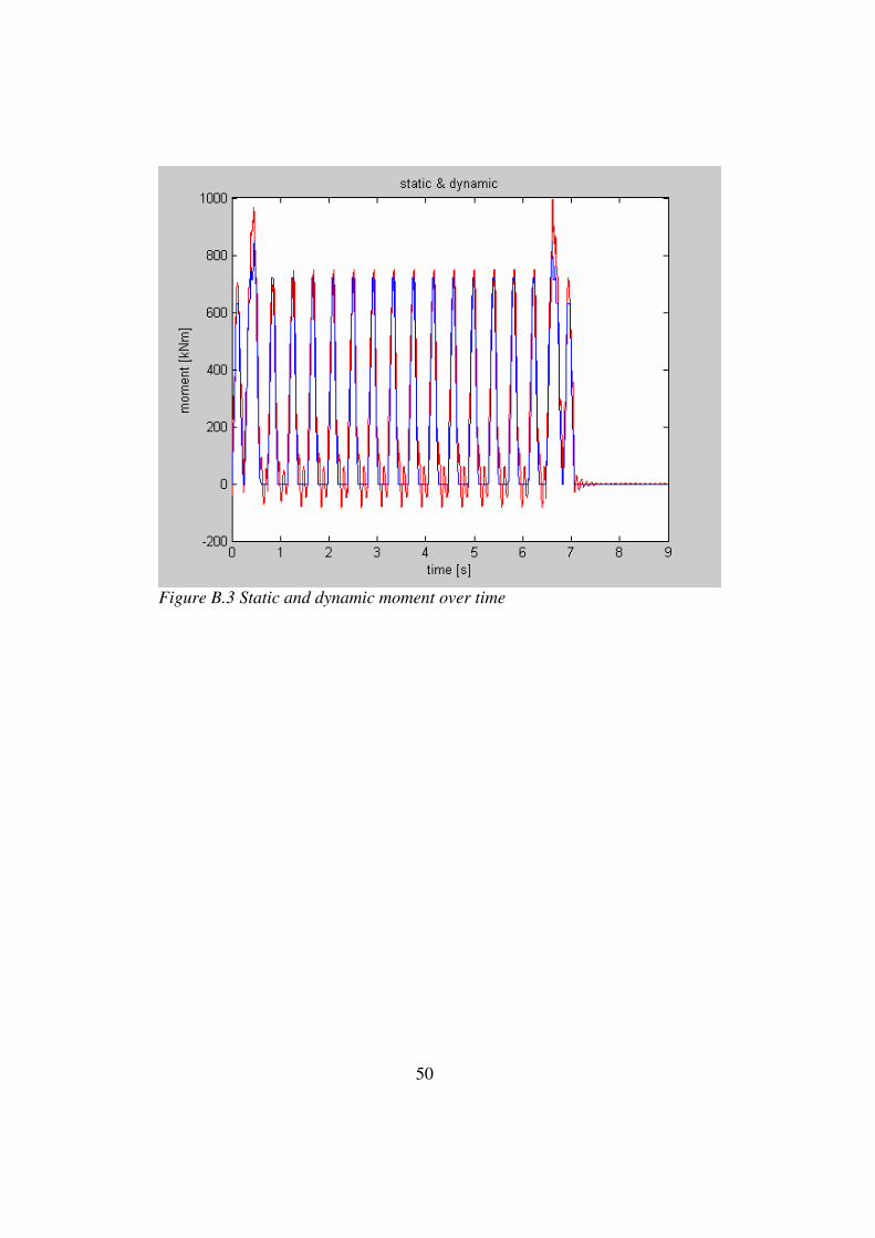
even numbered. The dynamic mid span moment are determined for the same time steps as for the static moment. The diagrams in appendix B illustrates the time variation of the static mid span moment, Figure B.1, the dynamic mid span moment, Figure B.2 and both the static and dynamic mid span moment, is depicted in Figure B.3.

20
21
4 Parametric study
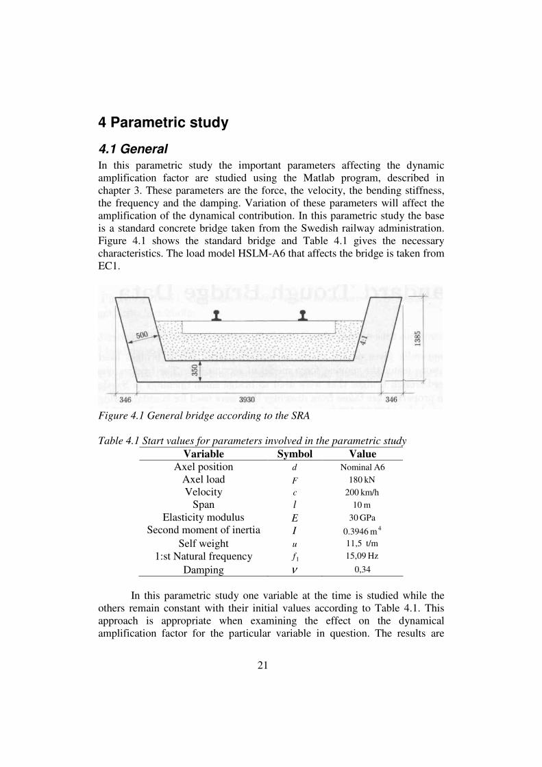
4.1 General In this parametric study the important parameters affecting the dynamic amplification factor are studied using the Matlab program, described in chapter 3. These parameters are the force, the velocity, the bending stiffness, the frequency and the damping. Variation of these parameters will affect the amplification of the dynamical contribution. In this parametric study the base is a standard concrete bridge taken from the Swedish railway administration. Figure 4.1 shows the standard bridge and Table 4.1 gives the necessary characteristics. The load model HSLM-A6 that affects the bridge is taken from EC1.
Figure 4.1 General bridge according to the SRA
Table 4.1 Start values for parameters involved in the parametric study
Variable Symbol Value
Axel position d A6 Nominal Axel load F kN 180 Velocity c km/h 200
Span l m 10 Elasticity modulus E GPa 30
Second moment of inertia I 4m 3946.0 Self weight u t/m11,5
1:st Natural frequency 1f Hz 15,09
Damping ν 0,34
In this parametric study one variable at the time is studied while the
others remain constant with their initial values according to Table 4.1. This approach is appropriate when examining the effect on the dynamical amplification factor for the particular variable in question. The results are
22
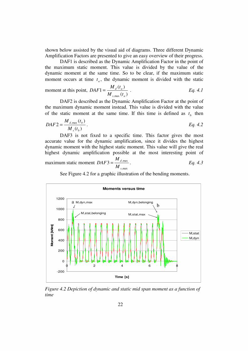
shown below assisted by the visual aid of diagrams. Three different Dynamic Amplification Factors are presented to give an easy overview of their progress.
DAF1 is described as the Dynamic Amplification Factor in the point of the maximum static moment. This value is divided by the value of the dynamic moment at the same time. So to be clear, if the maximum static moment occurs at time at , the dynamic moment is divided with the static
moment at this point, )(
)(1
max, as
ad
tM
tMDAF = . Eq. 4.1
DAF2 is described as the Dynamic Amplification Factor at the point of the maximum dynamic moment instead. This value is divided with the value of the static moment at the same time. If this time is defined as bt then
)(
)(2 max,
bs
bd
tM
tMDAF = . Eq. 4.2
DAF3 is not fixed to a specific time. This factor gives the most accurate value for the dynamic amplification, since it divides the highest dynamic moment with the highest static moment. This value will give the real highest dynamic amplification possible at the most interesting point of
maximum static moment max,
max,3
s
d
M
MDAF = . Eq. 4.3
See Figure 4.2 for a graphic illustration of the bending moments.
Figure 4.2 Depiction of dynamic and static mid span moment as a function of
time
Moments versus time
-200
0
200
400
600
800
1000
1200
0 2 4 6 8
Time [s]
Mom
ent [k
Nm
]
M,stat
M,dyn
M,dyn,max
M,stat,belonging M,stat,max
M,dyn,belonging
b a

23
DAF1 and DAF2 are examined to give a wider knowledge of the dynamic amplification but the only DAF3 is of real interest for a structural engineer.
As seen in the diagrams the static moment does only increase when increasing the force. The dynamic moment increases with higher force and velocity but decreases with higher bending stiffness, frequency and remaining constant even though slightly decreasing for the damping.
Span length is obviously of such a great importance that it is not introduced in the parameter study. Instead it is embedded in the final examination with different common lengths to form a vital part of the results.

24
4.2 Force The force is obviously the most important factor when dealing with static moments, but this is not the case for dynamic moments. The dynamic moment is always slightly higher than the static moment with a dynamic amplification factor around 1.18 for DAF3. If it would be a frog bouncing on the bridge, this would give impulses in the bridge thus a higher force probably would result in a higher dynamic response (No frogs are studied in this thesis) but since the train results in a linear force spectra, any kind of force amplitude absorbs the bridge’s dynamic response, induced by it self. Naturally it follows that if the force is higher the response will be higher and the dynamic amplification almost constant. The important thing is consequently to make sure that the bridge can manage the static moment with the additional dynamic moment. The diagram in Figure 4.3 for the dynamic amplification factors shows fluctuating curves but the dynamic amplification factors are all under 1.30, which can be considered as a low dynamic impact. The low dynamic influence from the force is also obvious when examining the moment diagram in Figure 4.4, where the static mid span bending moment does not differ much from the dynamic mid span bending moment.
Dynamic amplification versus force
1,00
1,10
1,20
1,30
90 108 126 144 162 180 198 216 234 252 270
F [kN]
DA
F
DAF1
DAF2
DAF3
Figure 4.3 The three different dynamic amplification factors as a function of
the force

25
Static and dynamic moment versus force
200
400
600
800
1000
1200
1400
1600
1800
0 50 100 150 200 250 300
F [kN]
M [kN
m]
Ms
Md
Figure 4.4 Maximum static and dynamic mid span bending moment in a
simply supported bridge of 10 meters.
4.3 Velocity The reason for this study is because the train is moving, Static = still, dynamic = in motion, hence the most important parameter, when dealing with dynamic effects in railway bridges, is the motion of the train. Of course, as shown in figure 4.5, the motion of the train is by far the most important, when dealing with the general bridge studied in this paper.
Dynamic amplification versus velocity
0,91,01,11,21,31,41,51,61,71,81,92,0
0 100 200 300 400
c [km/h]
DA
F
DAF1
DAF2
DAF3
Figure 4.5 The three different dynamic amplification factors as a function of
the velocity
26
Static and dynamic moment versus velocity
600
800
1000
1200
1400
1600
1800
0 100 200 300 400
c [km/h]
M [
kN
m]
Ms
Md
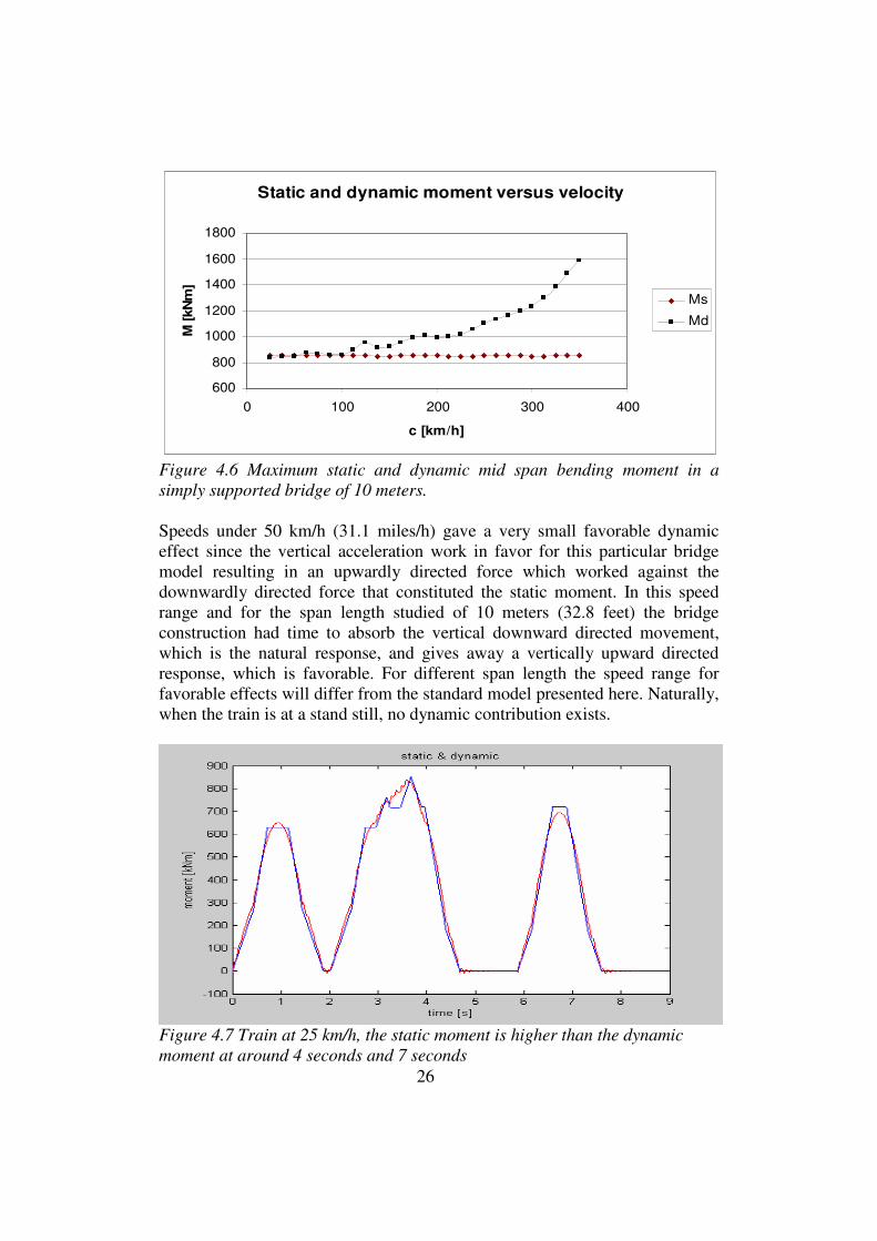
Figure 4.6 Maximum static and dynamic mid span bending moment in a
simply supported bridge of 10 meters.
Speeds under 50 km/h (31.1 miles/h) gave a very small favorable dynamic effect since the vertical acceleration work in favor for this particular bridge model resulting in an upwardly directed force which worked against the downwardly directed force that constituted the static moment. In this speed range and for the span length studied of 10 meters (32.8 feet) the bridge construction had time to absorb the vertical downward directed movement, which is the natural response, and gives away a vertically upward directed response, which is favorable. For different span length the speed range for favorable effects will differ from the standard model presented here. Naturally, when the train is at a stand still, no dynamic contribution exists.
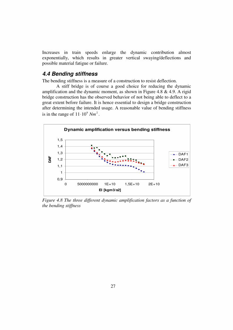
Figure 4.7 Train at 25 km/h, the static moment is higher than the dynamic
moment at around 4 seconds and 7 seconds
27
Increases in train speeds enlarge the dynamic contribution almost exponentially, which results in greater vertical swaying/deflections and possible material fatigue or failure.
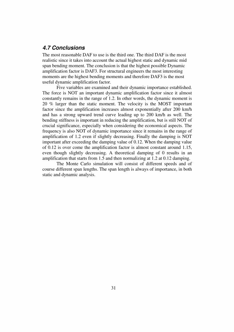
4.4 Bending stiffness The bending stiffness is a measure of a construction to resist deflection.
A stiff bridge is of course a good choice for reducing the dynamic amplification and the dynamic moment, as shown in Figure 4.8 & 4.9. A rigid bridge construction has the observed behavior of not being able to deflect to a great extent before failure. It is hence essential to design a bridge construction after determining the intended usage. A reasonable value of bending stiffness
is in the range of 291011 Nm⋅ .
Dynamic amplification versus bending stiffness
0,9
1
1,1
1,2
1,3
1,4
1,5
0 5000000000 1E+10 1,5E+10 2E+10
EI [kgm3/s2]
DA
F
DAF1
DAF2
DAF3
Figure 4.8 The three different dynamic amplification factors as a function of
the bending stiffness

28
Static and dynamic moment versus bending
stiffness
800850
900950
10001050
11001150
1200
0,00E+00 5,00E+09 1,00E+10 1,50E+10 2,00E+10
EI [kgm3/s2]
M [
kN
m]
Ms
Md
Figure 4.9 Maximum static and dynamic mid span bending moment in a
simply supported bridge of 10 meters.
4.5 Frequency Every material has its own natural frequency which also depends on its form. A moving load, e.g. a crowd of people walking on a bridge, wind load acting on a bridge, or even a train passing over a bridge can bring the bridge into a swaying motion, equal to the bridges natural frequency, which makes it more vulnerable to fatigue. At the point of the construction’s natural frequency, the construction will come into an enhanced sway which with a persistent critical loading which causes the construction to collapse. Therefore the natural frequency is a very important safety parameter. The natural frequency can be estimated as a function of the mass and the bending stiffness. The Tacoma bridge collapse is an important example of how natural frequencies can lead to disaster (Fuller, 1982).

29
Dynamic amplification versus frequency
1
1,1
1,2
1,3
1,4
0 5 10 15 20 25 30
f [Hz]
DA
F
DAF1
DAF2
DAF3
Figure 4.10 The three different dynamic amplification factors as a function of
the frequency
Static and dynamic moment versus frequency
800
850
900
950
1000
1050
0 5 10 15 20 25 30
f [Hz]
M [
kN
m]
Ms
Md
Figure 4.11 Maximum static and dynamic mid span bending moment in a
simply supported bridge of 10 meters.
4.6 Damping One of the most important variables to consider in earthquake engineering is damping. In some parts of Europe earthquakes are a prevalent danger which requires special consideration in design. Damping is also an important parameter when reducing regular dynamic effects (Elnashai, 2005).
To avoid over stressing and damage of bridges elastic rubber bearing pads can be used as a damping material. Damping is important because it reduces reaction forces and bending movements, if installed properly a

30
damping material should isolate and absorb vibration from lateral movements without transmitting stresses.
Figure 4.12 shows a high value, with a damping value of 0. It is of importance to recognize that a damping value of 0 is theoretical and is not applicable in practice. The damping does not have a significant effect after a critical damping value of around 0.15.
Dynamic amplification versus damping
1
1,1
1,2
1,3
1,4
1,5
1,6
1,7
1,8
1,9
0 0,1 0,2 0,3 0,4 0,5 0,6 0,7 0,8 0,9 1 1,1
v
DA
F
DAF1
DAF2
DAF3
Figure 4.12 The three different dynamic amplification factors as a function of
the damping
Static and dynamic moment versus damping
800
900
1000
1100
1200
1300
1400
0 0,2 0,4 0,6 0,8 1 1,2
v
M
Ms
Md
Figure 4.13 Maximum static and dynamic mid span bending moment in a
simply supported bridge of 10 meters.
31
4.7 Conclusions The most reasonable DAF to use is the third one. The third DAF is the most realistic since it takes into account the actual highest static and dynamic mid span bending moment. The conclusion is that the highest possible Dynamic amplification factor is DAF3. For structural engineers the most interesting moments are the highest bending moments and therefore DAF3 is the most useful dynamic amplification factor.
Five variables are examined and their dynamic importance established. The force is NOT an important dynamic amplification factor since it almost constantly remains in the range of 1.2. In other words, the dynamic moment is 20 % larger than the static moment. The velocity is the MOST important factor since the amplification increases almost exponentially after 200 km/h and has a strong upward trend curve leading up to 200 km/h as well. The bending stiffness is important in reducing the amplification, but is still NOT of crucial significance, especially when considering the economical aspects. The frequency is also NOT of dynamic importance since it remains in the range of amplification of 1.2 even if slightly decreasing. Finally the damping is NOT important after exceeding the damping value of 0.12. When the damping value of 0.12 is over come the amplification factor is almost constant around 1.15, even though slightly decreasing. A theoretical damping of 0 results in an amplification that starts from 1.5 and then normalizing at 1.2 at 0.12 damping.
The Monte Carlo simulation will consist of different speeds and of course different span lengths. The span length is always of importance, in both static and dynamic analysis.

32

33
5 Statistical evaluation
5.1 Introduction In reliability analyses of different types of structures a statistical description of all the variables involved in the limit state function is necessary. The traffic load on railway bridges is the most dominating variable load and has therefore large influence on the result in analysis of railway bridges. This is a motivation to get better knowledge of this random variable. The train load is divided into two parts, a static and a dynamic part. Focus in this thesis is kept on the dynamic part. The purpose of this chapter is to investigate how the dynamic amplification factor is statistically distributed. To enable an investigation of the statistical distribution a method called Monte Carlo simulation is used, for information about the method the author refers to Melchers (1999).
5.2 Monte Carlo simulation The Monte Carlo simulation is a useful tool, since it randomly generates values for uncertain variables repeatedly to build up a reliable model. The model randomly picks values from the decided distributions in the statistical parameter composition and presents the results. The model is used to minimize uncertainty during the life time of the bridge construction. It can be explained as a technique of statistical sampling used to approximate solutions to quantitative problems, where the quantity is the number of train passes over a bridge for the entire expected lifespan of the bridge. Numerical modeling is a much needed tool when a physical experimentation data is difficult to obtain, since this thesis would take 50-100 years of observation and trains will probably fly by then, this is not really an option. The computer code used for the Monte Carlo simulation can be seen in Appendix C.
5.3 Statistical parameter composition The random variable composition is chosen according to equations 5.1 to 5.5. There are no rules for which distribution is the best for most variables, since they have not been investigated. The variables have to be connected with a distribution depending on which of the distributions fits the closest to the reality. The statistical randomness is vital to the description of the whole process where a train traverses a railway bridge. The variables in equation 5.1 to 5.5 will be used to simulate a general event of train traffic on a bridge using the Monte Carlo simulation. Each variable is connected with a probability distribution.
34
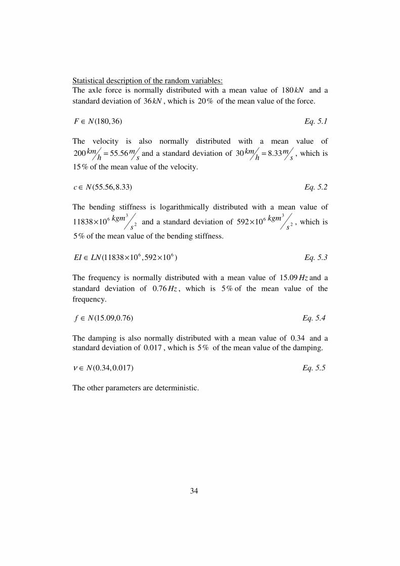
Statistical description of the random variables: The axle force is normally distributed with a mean value of kN180 and a
standard deviation of kN36 , which is %20 of the mean value of the force.
)36,180(NF ∈ Eq. 5.1
The velocity is also normally distributed with a mean value of
sm
hkm 56.55200 = and a standard deviation of
sm
hkm 33.830 = , which is
%15 of the mean value of the velocity.
)33.8,56.55(Nc ∈ Eq. 5.2
The bending stiffness is logarithmically distributed with a mean value of
2
361011838
skgm
× and a standard deviation of 2
3610592
skgm
× , which is
%5 of the mean value of the bending stiffness.
)10592,1011838( 66 ××∈ LNEI Eq. 5.3
The frequency is normally distributed with a mean value of Hz09.15 and a
standard deviation of Hz76.0 , which is %5 of the mean value of the
frequency.
)76.0,09.15(Nf ∈ Eq. 5.4
The damping is also normally distributed with a mean value of 34.0 and a standard deviation of 017.0 , which is %5 of the mean value of the damping.
)017.0,34.0(N∈ν Eq. 5.5
The other parameters are deterministic.
35
5.4 Goodness of fit To assist with clarification, the results from the simulation diagrams of the static and dynamic moments will be shown. The results will be compared with the normal and lognormal distribution to analyze how compatible they are to these curves. The mean square distance, MSE (Montgomery, D, 1997) is a measure of the variation for the empirical model and the chosen model given by:
( )( )
1
ˆ)(1
2
−
−
=
∑=
n
xFxF
MSE
n
j
ii
Eq. 5.6
where F is the theoretical distribution function and F̂ is the empirical distribution function. n is the number of trains traversing the bridge.
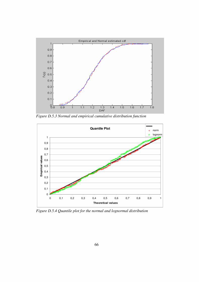
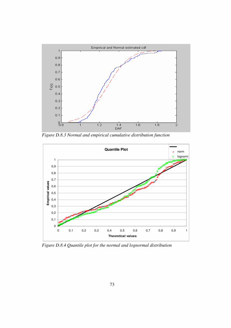
A quantile plot will further enhance the understanding of which distribution is the closest to the reality. The estimated values are here compared with the theoretical values and mean square distance value from the diagonal line will be shown to even further enhance the analysis of which distribution is the most accurate. Several quantile plots are presented in Appendix D.

36
37
6 Dynamic Amplification Factors
6.1 Introduction The dynamic amplification factor is a relative measure of the importance of the dynamic impact. Short span bridges can withstand very high velocities with a low level of influence. The short span bridges have a natural character which resists vertical accelerations compared to the long span bridges which are easier to induce into a vertical movement, for these types of bridges. As shown in Table 6.1 and Table 6.2 the dynamic amplification factors mean value is less than 1.2 for spans up to 10 meters and velocities up to 200 km/h. The interesting finding is that the Table 6.1 and 6.2 shows how different the values are for different spans and different velocities.
To assist with comprehension of the results it is important to understand that this is a general Swedish bridge taken from the Swedish rail road administration and therefore it is not designed for high speed trains, which becomes apparent when the 20 meter span bridge with a velocity of 250 km/h is studied. The bridge in its current configuration will probably not be able to withstand a dynamic amplification impact of around 2, if it is not considered when designing the bridge. The magnitude of the dynamic amplification factor is in it self also an important confirmation of how significant the dynamic effects are. Interesting is also the dynamic amplification for longer spans, by studying figure D.11.1 for example, when it becomes apparent that the bridge has no time to respond with a peaking dynamic amplification. This is due to the span length and the train coach length. Before the bridge has any possibility to respond in an accentuated peak the next axle is loaded on the bridge and therefore the dynamic impulses are more concentrated in the middle of the bridge with increased speed and span length. After the train has finished traversing the bridge, the magnitude of the dynamic impact is obvious. The after vibrations inducted in the bridge are large, with higher peaks for higher velocities. Figure 6.1 shows an example of the after vibrations inducted in the bridge when the train has finished traversing it.

38
Figure 6.1 Example of long span bridge of 20 meters being traversed by a
high speed train, Static and dynamic mid span bending moment
The final results are presented below, which help in displaying the importance of the dynamic effects on a bridge. This standard bridge is not constructed for high speeds and with a span of 20 meters and a velocity of 250 km/h the bridge would probably fail.
Moments versus time
-1000
-500
0
500
1000
1500
2000
2500
3000
3500
0 2 4 6 8 10
Time [s]
Mom
ent [k
Nm
]
M,stat
M,dyn
M,dyn,max
M,stat,maxM,stat,belonging
M,dyn,belonging

39
6.2 Final results Table 6.1 Final results of the dynamic amplification factors, Normal
distribution
DAF
Span Length (m)
Velocity (km/h) 5 10 15 20
150 1.013 1.117 1.199 1.1981
200 1.037 1.195 1.279 1.352
250 1.031 1.330 1.402 2.062
Variance
Span Length (m)
Velocity (km/h) 5 10 15 20
150 0.1375 0.1353 0.1487 0.1575
200 0.1296 0.1513 0.1847 0.3095
250 0.1308 0.2133 0.2291 0.7316
Table 6.2 Final results of the dynamic amplification factors, Lognormal
distribution
DAF
Span Length (m)
Velocity (km/h) 5 10 15 20
150 1.004 1.109 1.199 1.188
200 1.030 1.185 1.266 1.323
250 1.023 1.314 1.385 1.95
Variance
Span Length (m)
Velocity (km/h) 5 10 15 20
150 0.134 0.1191 0.1225 0.1281
200 0.122 0.1257 0.1382 0.2027
250 0.125 0.1552 0.1575 0.3262
After examination of Table 6.3 and Table 6.4 one can see that the appropriate distribution for small spans and low speed is the lognormal distribution but it does not follow an easy to explain pattern, since the 20 meter span, 200 km/h simulation shows that the lognormal distribution is the closest to the reality.

40
Table 6.3 MSE factor for the normal distribution
Span Length (m)
Velocity (km/h) 5 10 15 20
150 0,000725 0,000765 0,000998 0,000727
200 0,000916 0,000233 0,003721 0,006339
250 0,000474 0,001186 0,00059 0,013689
Table 6.4 MSE factor for the lognormal distribution
Span Length (m)
Velocity (km/h) 5 10 15 20
150 0,000411 0,000732 0,001356 0,000914
200 0,000379 0,001289 0,003902 0,003918
250 0,000258 0,00214 0,003638 0,037969
In an overall average the normal distribution can better describe these phenomena with a value of 0,002530 compared with the lognormal distributions value of 0,004742.
6.3 Conclusions To reduce the dynamic effects imposed on a bridge it is possible to use the damping and the bending stiffness and also the frequency that are a function of the bending stiffness and mass. It is possible to build bridges that can withstand high velocity trains, if they are designed in an accurate manner. High velocity trains are already in use in Germany, Japan and China for example. Span lengths and velocity impact on bridges are very important to understand, when constructing a bridge appropriate for high velocity trains, and one should also have a wide understanding of the safety and security from both the technical and human perspectives. The tracks should be periodically and carefully maintained to minimize risks. In Germany an accident occurred on the 24 of September 2006 involving a high velocity train, the Transrapid (Daily newspaper, La Repubblica). This was due to a track maintenance vehicle being left on the tracks. Human errors should of course also be brought into the security thinking. In China high speed trains travel from Shanghai to the airport in Pudong at speeds of up to 430 km/h, so it can be seen as a good option instead of driving, from an environmental point of view as well. When designing bridges the vertical forces are not to be neglected, though especially from a static point of view. The resonance effect is also a vital variable which if neglected could and have caused disasters. Several accidents have occurred due to the resonance effect imposed by wind load as well as other loads.

41
Finally taking economy into consideration, which is of course always an important parameter, an economically justified and well-designed bridge, appropriate for high speed trains can be constructed with assistance from reliable dynamic amplification factors.

42
References
Code: Eurocode 1: Actions on structures, Traffic load on bridges,
European standard 2002
Code: BV Bro 2004, release 7 (utgåva 7), Swedish bridge design code,
(Banverkets ändringar och tillägg till vägverkets Bro 2004)
Institute: Swedish rail road administration, (Banverket)
Paper: Paper 76, Stress ranges in bridges under high speed trains, Civil-
Comp Ltd. Stirling Scotland. Proceedings of the ninth International
Conference on Civil and Structural Engineering Computing, B.H.V.
Topping (Editor), Civil Comp Press, Stirling, Scotland, L. Frýba, C.
Fischer and J-D. Yau, 2003.
Course literature: Amr. Elnashai and Luigi Di Sarno, CEE-572
Earthquake engineering, Introduction to earthquake structural engineering,
Fall 2005, University of Illinois at Urbana-Champaign
Book: Robert G. Fuller, The Puzzle of the Tacoma Narrows Bridge
Collapse, 1982, Wiley, ISBN 0 471 87320 9
Book: Robert E. Melchers, Structural Reliability Analysis and Prediction,
second edition, 1999, John Wiley & Sons, The University of Newcastle,
Australia, ISBN 0 471 98771 9 (Pr)
Book: Montgomery, D, Design and analysis of experiments. Wiley &
Sons, Inc. ISBN 0 471 15746 5

43
Daily newspaper: La Repubblica, www.repubblica.it 2006-09-24

44
Appendix
A Matlab code
B Figures Matlab
C Monte Carlo simulation
D Figures Monte Carlo
45
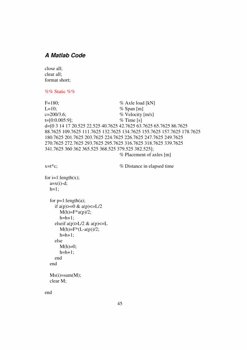
A Matlab Code close all; clear all; format short; %% Static %% F=180; % Axle load [kN] L=10; % Span [m] c=200/3.6; % Velocity [m/s] t=[0:0.005:9]; % Time [s] d=[0 3 14 17 20.525 22.525 40.7625 42.7625 63.7625 65.7625 86.7625 88.7625 109.7625 111.7625 132.7625 134.7625 155.7625 157.7625 178.7625 180.7625 201.7625 203.7625 224.7625 226.7625 247.7625 249.7625 270.7625 272.7625 293.7625 295.7625 316.7625 318.7625 339.7625 341.7625 360 362 365.525 368.525 379.525 382.525]; % Placement of axles [m] x=t*c; % Distance in elapsed time for i=1:length(x); a=x(i)-d; h=1; for p=1:length(a); if a(p)>=0 & a(p)<=L/2 M(h)=F*a(p)/2; h=h+1; elseif a(p)>L/2 & a(p)<=L M(h)=F*(L-a(p))/2; h=h+1; else M(h)=0; h=h+1; end end Ms(i)=sum(M); clear M; end
46
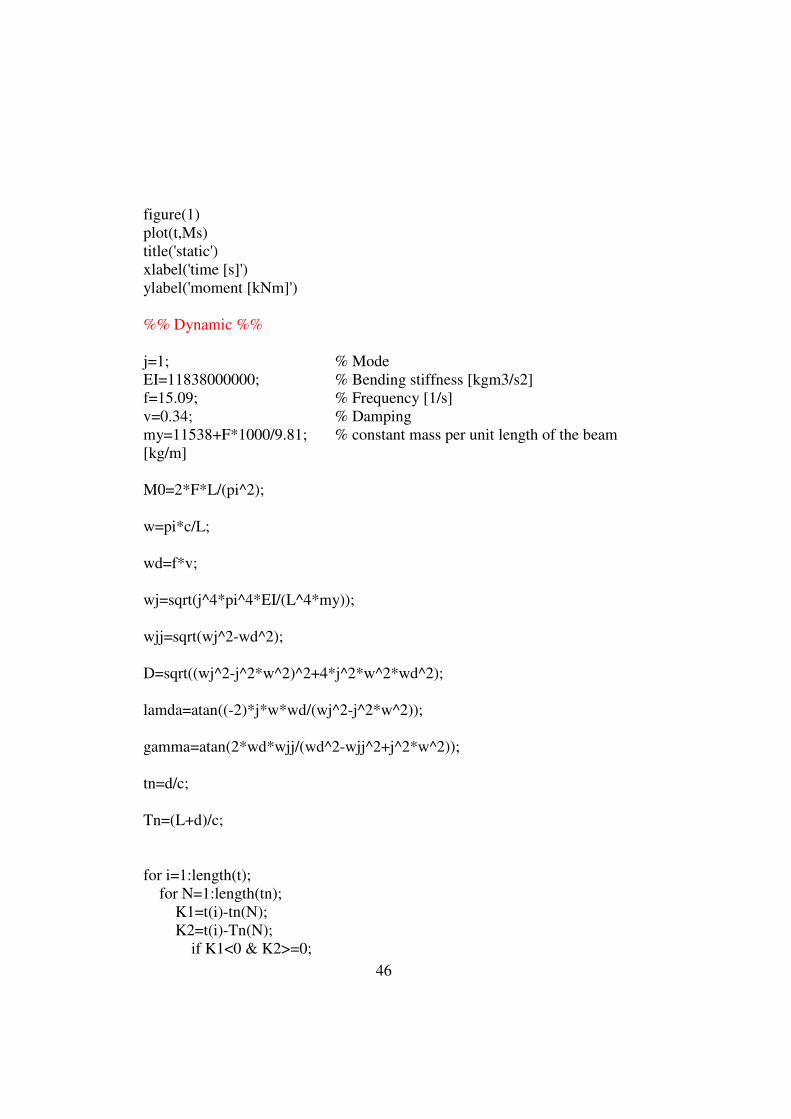
figure(1) plot(t,Ms) title('static') xlabel('time [s]') ylabel('moment [kNm]') %% Dynamic %% j=1; % Mode EI=11838000000; % Bending stiffness [kgm3/s2] f=15.09; % Frequency [1/s] v=0.34; % Damping my=11538+F*1000/9.81; % constant mass per unit length of the beam [kg/m] M0=2*F*L/(pi^2); w=pi*c/L; wd=f*v; wj=sqrt(j^4*pi^4*EI/(L^4*my)); wjj=sqrt(wj^2-wd^2); D=sqrt((wj^2-j^2*w^2)^2+4*j^2*w^2*wd^2); lamda=atan((-2)*j*w*wd/(wj^2-j^2*w^2)); gamma=atan(2*wd*wjj/(wd^2-wjj^2+j^2*w^2)); tn=d/c; Tn=(L+d)/c; for i=1:length(t); for N=1:length(tn); K1=t(i)-tn(N); K2=t(i)-Tn(N); if K1<0 & K2>=0;

47
h1=0; f1(N)=0; h2=1; f2(N)=1/(wjj*D)*(wjj/(j*w)*sin(j*w*K2+lamda)+ exp(-wd*K2)*sin(wjj*K2+gamma)); elseif K1>=0 & K2>=0; h1=1; f1(N)=1/(wjj*D)*(wjj/(j*w)*sin(j*w*K1+lamda)+ exp(-wd*K1)*sin(wjj*K1+gamma)); h2=1; f2(N)=1/(wjj*D)*(wjj/(j*w)*sin(j*w*K2+lamda)+ exp(-wd*K2)*sin(wjj*K2+gamma)); elseif K1>=0 & K2<0; h1=1; f1(N)=1/(wjj*D)*(wjj/(j*w)*sin(j*w*K1+lamda)+ exp(-wd*K1)*sin(wjj*K1+gamma)); h2=0; f2(N)=0; else K1<0 & K2<0; h1=0; f1(N)=0; h2=0; f2(N)=0; end ftot(N)=f1(N)*h1-(-1)^j*f2(N)*h2; end fp=1/(wjj*D)*(wjj/(j*w)*sin(j*w*t+lamda)+exp(-wd*t).*sin(wjj*t+gamma)); Md(i)=M0*j^3*w*wj^2*sum(ftot)*sin(j*pi/2); clear M; end figure(2) plot(t,Md) title('dynamic') xlabel('time [s]')

48
ylabel('moment [kNm]') figure(3) plot(t,Md,'r') hold on plot(t,Ms,'b') hold off title('static & dynamic') xlabel('time [s]') ylabel('moment [kNm]') [a,b]=max(Ms); DAF1=Md(b)/max(Ms) [a,b]=max(Md); DAF2=max(Md)/Ms(b) DAF3=max(Md)/max(Ms) max(Ms) max(Md)

49
B Figures Matlab
Figure B.1 Static moment over time
Figure B.2 Dynamic moment over time
50
Figure B.3 Static and dynamic moment over time
51
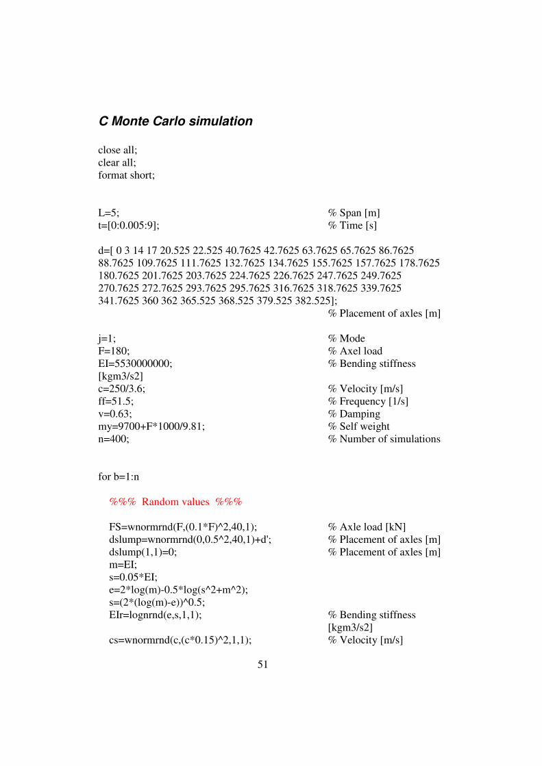
C Monte Carlo simulation close all; clear all; format short; L=5; % Span [m] t=[0:0.005:9]; % Time [s] d=[ 0 3 14 17 20.525 22.525 40.7625 42.7625 63.7625 65.7625 86.7625 88.7625 109.7625 111.7625 132.7625 134.7625 155.7625 157.7625 178.7625 180.7625 201.7625 203.7625 224.7625 226.7625 247.7625 249.7625 270.7625 272.7625 293.7625 295.7625 316.7625 318.7625 339.7625 341.7625 360 362 365.525 368.525 379.525 382.525];
% Placement of axles [m] j=1; % Mode F=180; % Axel load EI=5530000000; % Bending stiffness [kgm3/s2] c=250/3.6; % Velocity [m/s] ff=51.5; % Frequency [1/s] v=0.63; % Damping my=9700+F*1000/9.81; % Self weight n=400; % Number of simulations for b=1:n %%% Random values %%% FS=wnormrnd(F,(0.1*F)^2,40,1); % Axle load [kN] dslump=wnormrnd(0,0.5^2,40,1)+d'; % Placement of axles [m] dslump(1,1)=0; % Placement of axles [m] m=EI; s=0.05*EI; e=2*log(m)-0.5*log(s^2+m^2); s=(2*(log(m)-e))^0.5; EIr=lognrnd(e,s,1,1); % Bending stiffness
[kgm3/s2] cs=wnormrnd(c,(c*0.15)^2,1,1); % Velocity [m/s]
52
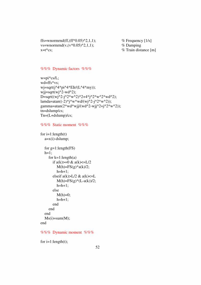
ffs=wnormrnd(ff,(ff*0.05)^2,1,1); % Frequency [1/s] vs=wnormrnd(v,(v*0.05)^2,1,1); % Damping x=t*cs; % Train distance [m] %%% Dynamic factors %%% w=pi*cs/L; wd=ffs*vs; wj=sqrt(j^4*pi^4*EIr/(L^4*my)); wjj=sqrt(wj^2-wd^2); D=sqrt((wj^2-j^2*w^2)^2+4*j^2*w^2*wd^2); lamda=atan((-2)*j*w*wd/(wj^2-j^2*w^2)); gamma=atan(2*wd*wjj/(wd^2-wjj^2+j^2*w^2)); tn=dslump/cs; Tn=(L+dslump)/cs; %%% Static moment %%% for i=1:length(t) a=x(i)-dslump; for g=1:length(FS) h=1; for k=1:length(a) if a(k)>=0 & a(k)<=L/2 M(h)=FS(g)*a(k)/2; h=h+1; elseif a(k)>L/2 & a(k)<=L M(h)=FS(g)*(L-a(k))/2; h=h+1; else M(h)=0; h=h+1; end end end Ms(i)=sum(M); end %%% Dynamic moment %%% for i=1:length(t);

53
for N=1:length(FS); K1=t(i)-tn(N); K2=t(i)-Tn(N); if K1<0 & K2>=0; f1(N)=0; f2(N)=1/(wjj*D)*((wjj/(j*w))*sin(j*w*K2+lamda)+exp(wd*K2)*sin(wjj*K2+gamma)); ftot(N)=(FS(N)*2*L/pi^2)*(f1(N)-(-1)^j*f2(N)); elseif K1>=0 & K2>=0; f1(N)=1/(wjj*D)*((wjj/(j*w))*sin(j*w*K1+lamda)+exp(-wd*K1)*sin(wjj*K1+gamma)); f2(N)=1/(wjj*D)*((wjj/(j*w))*sin(j*w*K2+lamda)+exp(-wd*K2)*sin(wjj*K2+gamma)); ftot(N)=(FS(N)*2*L/pi^2)*(f1(N)-(-1)^j*f2(N)); elseif K1>=0 & K2<0; f1(N)=1/(wjj*D)*((wjj/(j*w))*sin(j*w*K1+lamda)+exp(-wd*K1)*sin(wjj*K1+gamma)); f2(N)=0; ftot(N)=(FS(N)*2*L/pi^2)*(f1(N)-(-1)^j*f2(N)); else K1<0 & K2<0; f1(N)=0; f2(N)=0; ftot(N)=(FS(N)*2*L/pi^2)*(f1(N)-(-1)^j*f2(N)); end end Md(i)=sin(j*pi/2)*j*w*wj^2*sum(ftot); clear f1 f1 ftot end DAF(b)=max(Md)/max(Ms) end figure(1) plot(t,Ms,'b') hold on plot(t,Md,'r') title('Statit & Dynamic moment')

54
max(Ms) max(Md) figure(2) wlognfit(DAF) xlabel('DAF') ylabel('Fx(x)') figure(3) wnormfit(DAF) xlabel('DAF') ylabel('Fx(x)')
55
D Figures Monte Carlo
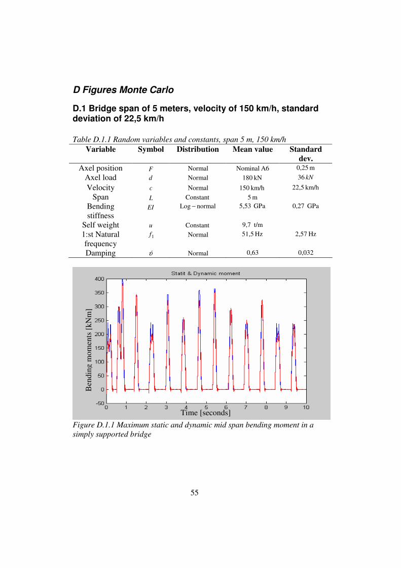
D.1 Bridge span of 5 meters, velocity of 150 km/h, standard deviation of 22,5 km/h
Table D.1.1 Random variables and constants, span 5 m, 150 km/h
Variable Symbol Distribution Mean value Standard
dev.
Axel position F Normal A6 Nominal m 0,25 Axel load d Normal kN 180 kN36
Velocity c Normal km/h 150 km/h 22,5 Span L Constant m 5
Bending stiffness
EI normalLog − GPa 5,53 GPa 0,27
Self weight u Constant t/m9,7 1:st Natural frequency
1f Normal Hz 51,5 Hz 2,57
Damping ϑ Normal 0,63 0,032
Figure D.1.1 Maximum static and dynamic mid span bending moment in a
simply supported bridge
Ben
ding
mom
ents
[kN
m]
Time [seconds]

56
Figure D.1.2 Lognormal and empirical cumulative distribution function
Figure D.1.3 Normal and empirical cumulative distribution function
57
Quantile Plot
0
0,1
0,2
0,3
0,4
0,5
0,6
0,7
0,8
0,9
1
0 0,1 0,2 0,3 0,4 0,5 0,6 0,7 0,8 0,9 1
Theoretical values
Em
pir
ical
valu
es
norm
lognorm
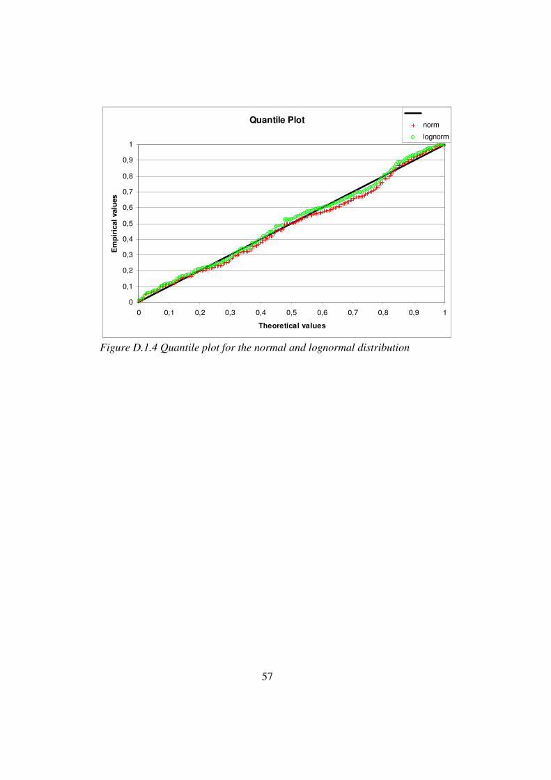
Figure D.1.4 Quantile plot for the normal and lognormal distribution
58
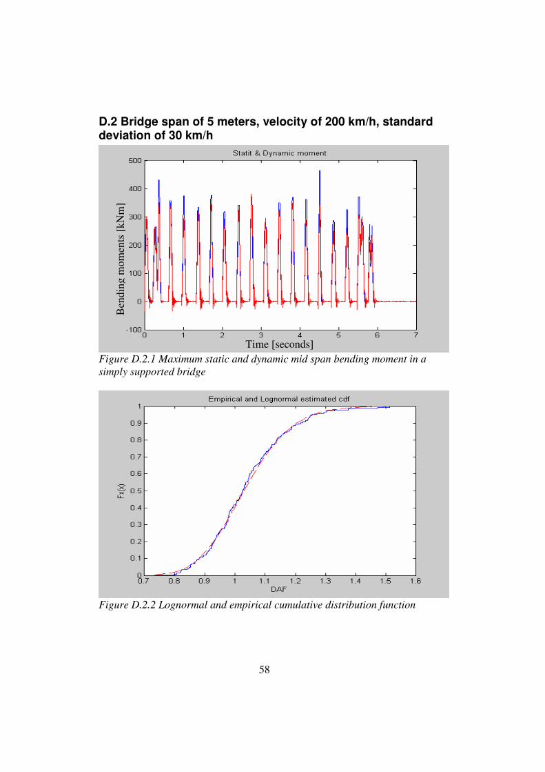
D.2 Bridge span of 5 meters, velocity of 200 km/h, standard deviation of 30 km/h
Figure D.2.1 Maximum static and dynamic mid span bending moment in a
simply supported bridge
Figure D.2.2 Lognormal and empirical cumulative distribution function
Ben
ding
mom
ents
[kN
m]
Time [seconds]

59
Figure D.2.3 Normal and empirical cumulative distribution function
Quantile Plot
0
0,1
0,2
0,3
0,4
0,5
0,6
0,7
0,8
0,9
1
0 0,1 0,2 0,3 0,4 0,5 0,6 0,7 0,8 0,9 1
Theoretical values
Em
pir
ical
valu
es
norm
lognorm
Figure D.2.4 Quantile plot for the normal and lognormal distribution

60
D.3 Bridge span of 5 meters, velocity of 250 km/h, standard deviation of 37,5 km/h
Figure D.3.1 Maximum static and dynamic mid span bending moment in a
simply supported bridge
Figure I.3.2 Lognormal and empirical cumulative distribution function
Ben
ding
mom
ents
[kN
m]
Time [seconds]

61
Figure I.3.3 Normal and empirical cumulative distribution function
Quantile Plot
0
0,1
0,2
0,3
0,4
0,5
0,6
0,7
0,8
0,9
1
0 0,1 0,2 0,3 0,4 0,5 0,6 0,7 0,8 0,9 1
Theoretical values
Em
pir
cal
valu
es
norm
lognorm
Figure I.3.4 Quantile plot for the normal and lognormal distribution
62
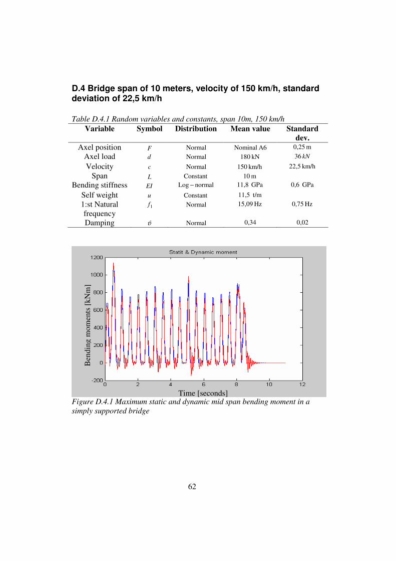
D.4 Bridge span of 10 meters, velocity of 150 km/h, standard deviation of 22,5 km/h
Table D.4.1 Random variables and constants, span 10m, 150 km/h
Variable Symbol Distribution Mean value Standard
dev.
Axel position F Normal A6 Nominal m 0,25 Axel load d Normal kN 180 kN36
Velocity c Normal km/h 150 km/h 22,5 Span L Constant m 10
Bending stiffness EI normalLog − GPa 11,8 GPa 0,6
Self weight u Constant t/m11,5 1:st Natural frequency
1f Normal Hz 15,09 Hz 0,75
Damping ϑ Normal 0,34 0,02
Figure D.4.1 Maximum static and dynamic mid span bending moment in a
simply supported bridge
Ben
ding
mom
ents
[kN
m]
Time [seconds]
63
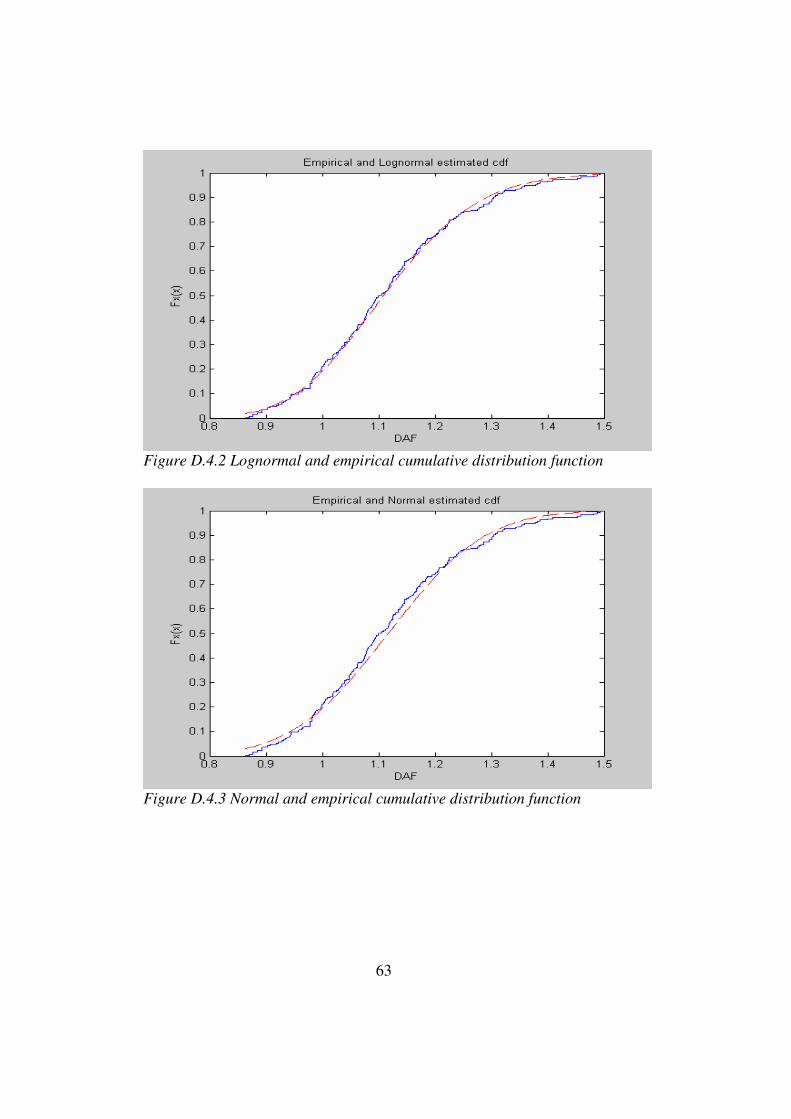
Figure D.4.2 Lognormal and empirical cumulative distribution function
Figure D.4.3 Normal and empirical cumulative distribution function

64
Quantile Plot
0
0,1
0,2
0,3
0,4
0,5
0,6
0,7
0,8
0,9
1
0 0,1 0,2 0,3 0,4 0,5 0,6 0,7 0,8 0,9 1
Theoretical values
Em
pir
ical
valu
es
norm
lognorm
Figure D.4.4 Quantile plot for the normal and lognormal distribution

65
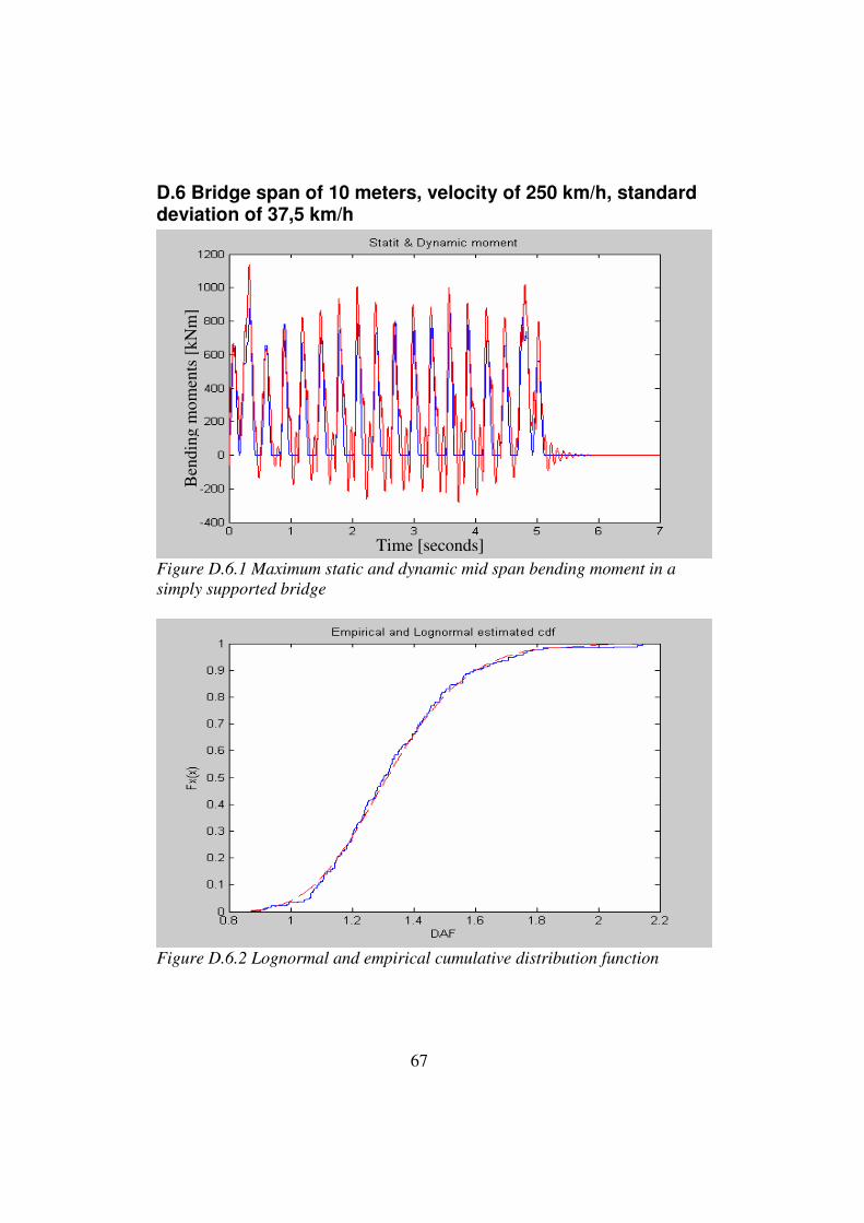
D.5 Bridge span of 10 meters, velocity of 200 km/h, standard deviation of 30 km/h
Figure D.5.1 Maximum static and dynamic mid span bending moment in a
simply supported bridge
Figure D.5.2 Lognormal and empirical cumulative distribution function
Time [seconds]
Ben
ding
mom
ents
[kN
m]
66
Figure D.5.3 Normal and empirical cumulative distribution function
Quantile Plot
0
0,1
0,2
0,3
0,4
0,5
0,6
0,7
0,8
0,9
1
0 0,1 0,2 0,3 0,4 0,5 0,6 0,7 0,8 0,9 1
Theoretical values
Em
pir
ical
valu
es
norm
lognorm
Figure D.5.4 Quantile plot for the normal and lognormal distribution
67
D.6 Bridge span of 10 meters, velocity of 250 km/h, standard deviation of 37,5 km/h
Figure D.6.1 Maximum static and dynamic mid span bending moment in a
simply supported bridge
Figure D.6.2 Lognormal and empirical cumulative distribution function
Ben
ding
mom
ents
[kN
m]
Time [seconds]

68
Figure D.6.3 Normal and empirical cumulative distribution function
Quantile Plot
0
0,1
0,2
0,3
0,4
0,5
0,6
0,7
0,8
0,9
1
0 0,1 0,2 0,3 0,4 0,5 0,6 0,7 0,8 0,9 1
Theoretical values
Em
pir
ical
valu
es
norm
lognorm
Figure D.6.4 Quantile plot for the normal and lognormal distribution

69
D.7 Bridge span of 15 meters, velocity of 150 km/h, standard deviation of 22,5 km/h
Table D.7.1 Random variables and constants, span 15m, 150 km/h
Variable Symbol Distribution Mean value Standard
dev.
Axel position F Normal A6 Nominal m 0,25 Axel load d Normal kN 180 kN36
Velocity c Normal km/h 150 km/h 22,5 Span L Constant m 15
Bending stiffness
EI normalLog − GPa 20,6 GPa 1,03
Self weight u Constant t/m12,4 1:st Natural frequency
1f Normal Hz 10,4 Hz 0,52
Damping ϑ Normal 0,26 0,013
Figure D.7.1 Maximum static and dynamic mid span bending moment in a
simply supported bridge
Ben
ding
mom
ents
[kN
m]
Time [seconds]
70
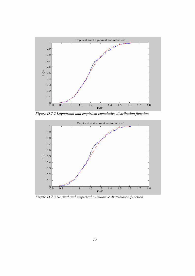
Figure D.7.2 Lognormal and empirical cumulative distribution function
Figure D.7.3 Normal and empirical cumulative distribution function

71
Quantile Plot
0
0,1
0,2
0,3
0,4
0,5
0,6
0,7
0,8
0,9
1
0 0,1 0,2 0,3 0,4 0,5 0,6 0,7 0,8 0,9 1
Theoretical values
Em
pir
ical
valu
es
norm
lognorm
Figure D.7.4 Quantile plot for the normal and lognormal distribution

72
D.8 Bridge span of 15 meters, velocity of 200 km/h, standard deviation of 22,5 km/h
Figure D.8.1 Maximum static and dynamic mid span bending moment in a
simply supported bridge
Figure D.8.2 Lognormal and empirical cumulative distribution function
Ben
ding
mom
ents
[kN
m]
Time [seconds]
73
Figure D.8.3 Normal and empirical cumulative distribution function
Quantile Plot
0
0,1
0,2
0,3
0,4
0,5
0,6
0,7
0,8
0,9
1
0 0,1 0,2 0,3 0,4 0,5 0,6 0,7 0,8 0,9 1
Theoretical values
Em
pir
ical
valu
es
norm
lognorm
Figure D.8.4 Quantile plot for the normal and lognormal distribution

74
D.9 Bridge span of 15 meters, velocity of 250 km/h, standard deviation of 37,5 km/h
Figure D.9.1 Maximum static and dynamic mid span bending moment in a
simply supported bridge
Figure D.9.2 Lognormal and empirical cumulative distribution function
Ben
ding
mom
ents
[kN
m]
Time [seconds]

75
Figure D.9.3 Normal and empirical cumulative distribution function
Quantile Plot
0
0,1
0,2
0,3
0,4
0,5
0,6
0,7
0,8
0,9
1
0 0,1 0,2 0,3 0,4 0,5 0,6 0,7 0,8 0,9 1
Theoretical values
Em
pir
ical
valu
es
norm
lognorm
Figure D.9.4 Quantile plot for the normal and lognormal distribution
76
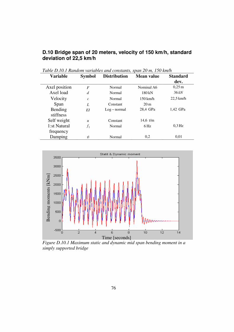
D.10 Bridge span of 20 meters, velocity of 150 km/h, standard deviation of 22,5 km/h
Table D.10.1 Random variables and constants, span 20 m, 150 km/h
Variable Symbol Distribution Mean value Standard
dev.
Axel position F Normal A6 Nominal m 0,25 Axel load d Normal kN 180 kN36
Velocity c Normal km/h 150 km/h 22,5 Span L Constant m 20
Bending stiffness
EI normalLog − GPa 28,4 GPa 1,42
Self weight u Constant t/m14,6 1:st Natural frequency
1f Normal Hz 6 Hz 0,3
Damping ϑ Normal 0,2 0,01
Figure D.10.1 Maximum static and dynamic mid span bending moment in a
simply supported bridge
Ben
ding
mom
ents
[kN
m]
Time [seconds]
77
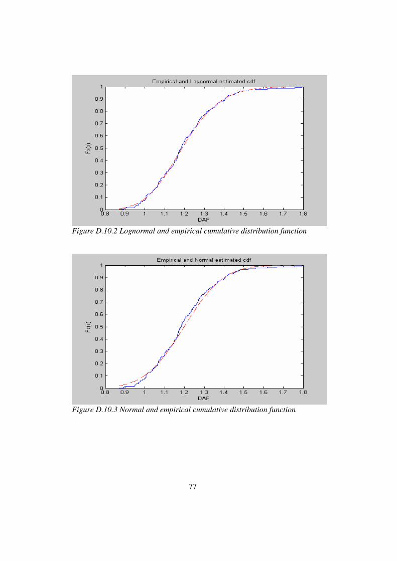
Figure D.10.2 Lognormal and empirical cumulative distribution function
Figure D.10.3 Normal and empirical cumulative distribution function

78
Quantile Plot
0
0,1
0,2
0,3
0,4
0,5
0,6
0,7
0,8
0,9
1
0 0,1 0,2 0,3 0,4 0,5 0,6 0,7 0,8 0,9 1
Theoretical values
Em
pir
ical
valu
es
norm
lognorm
Figure D.10.4 Quantile plot for the normal and lognormal distribution
79
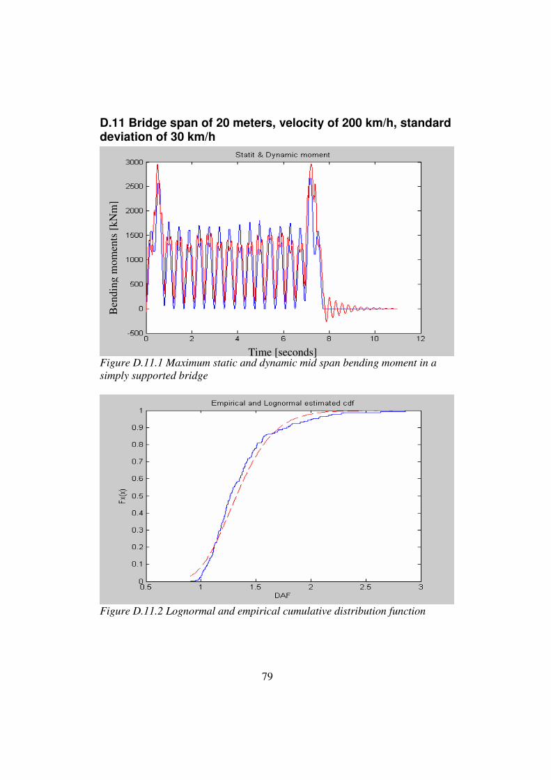
D.11 Bridge span of 20 meters, velocity of 200 km/h, standard deviation of 30 km/h
Figure D.11.1 Maximum static and dynamic mid span bending moment in a
simply supported bridge
Figure D.11.2 Lognormal and empirical cumulative distribution function
Ben
ding
mom
ents
[kN
m]
Time [seconds]
80
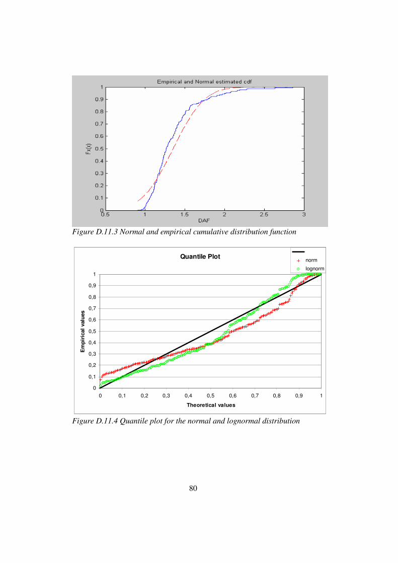
Figure D.11.3 Normal and empirical cumulative distribution function
Quantile Plot
0
0,1
0,2
0,3
0,4
0,5
0,6
0,7
0,8
0,9
1
0 0,1 0,2 0,3 0,4 0,5 0,6 0,7 0,8 0,9 1
Theoretical values
Em
pir
ical
valu
es
norm
lognorm
Figure D.11.4 Quantile plot for the normal and lognormal distribution
81
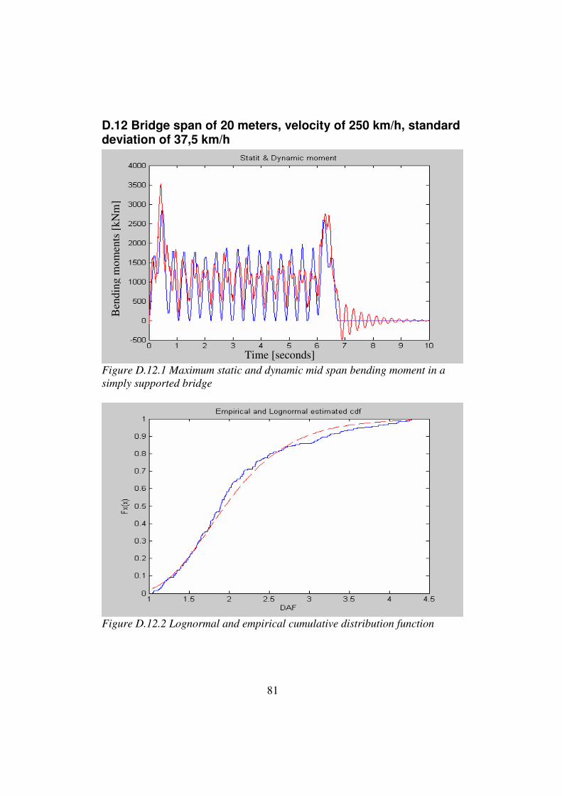
D.12 Bridge span of 20 meters, velocity of 250 km/h, standard deviation of 37,5 km/h
Figure D.12.1 Maximum static and dynamic mid span bending moment in a
simply supported bridge
Figure D.12.2 Lognormal and empirical cumulative distribution function
Ben
ding
mom
ents
[kN
m]
Time [seconds]
82
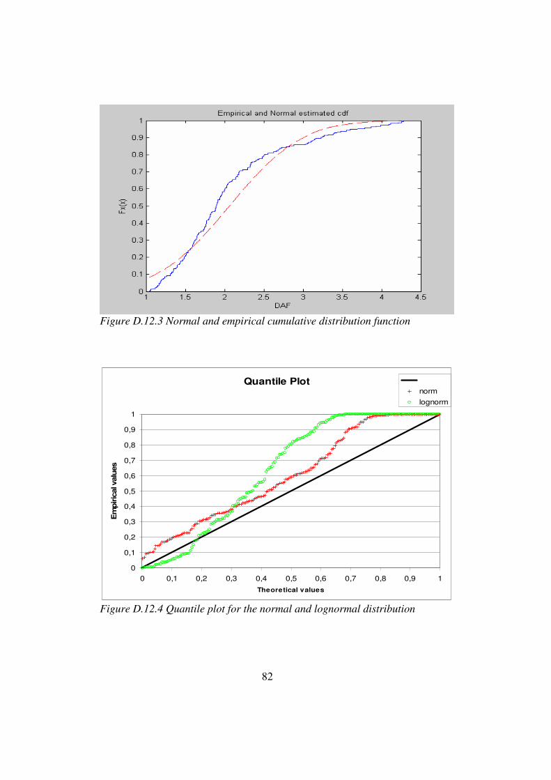
Figure D.12.3 Normal and empirical cumulative distribution function
Quantile Plot
0
0,1
0,2
0,3
0,4
0,5
0,6
0,7
0,8
0,9
1
0 0,1 0,2 0,3 0,4 0,5 0,6 0,7 0,8 0,9 1
Theoretical values
Em
piric
al valu
es
norm
lognorm
Figure D.12.4 Quantile plot for the normal and lognormal distribution