Master’s Degree Thesis Mechanical Engineering Influence ...940672/FULLTEXT02.pdf · As how it is...

Master’s Degree Thesis Mechanical Engineering

Supervisors: Ansel Berghuvud, BTH

Andreas Tyrberg, ABB

Influence Analysis of Coupling between

Tension and Torque in Single Armoured Cables

Joacim Malm

Blekinge Institute of Technology, Karlskrona, Sweden 2016

in collaboration with

Joacim Malm

Blekinge Institute of Technology Department of Mechanical Engineering

Karlskrona, Sweden 2016

Following thesis submitted for completion of Master of Science in Mechanical Engineering with emphasis on Structural Mechanics at Blekinge Institute of Technology, Karlskrona, Sweden.

Influence Analysis of Response Coupling between Tension and

Torque in Helically Single Armoured Cables

v

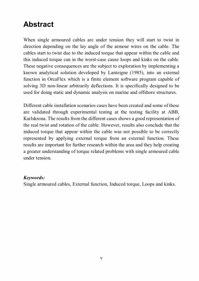
Abstract

When single armoured cables are under tension they will start to twist in direction depending on the lay angle of the armour wires on the cable. The cables start to twist due to the induced torque that appear within the cable and this induced torque can in the worst-case cause loops and kinks on the cable. These negative consequences are the subject to exploration by implementing a known analytical solution developed by Lanteigne (1985), into an external function in OrcaFlex which is a finite element software program capable of solving 3D non-linear arbitrarily deflections. It is specifically designed to be used for doing static and dynamic analysis on marine and offshore structures. Different cable installation scenarios cases have been created and some of these are validated through experimental testing at the testing facility at ABB, Karlskrona. The results from the different cases shows a good representation of the real twist and rotation of the cable. However, results also conclude that the induced torque that appear within the cable was not possible to be correctly represented by applying external torque from an external function. These results are important for further research within the area and they help creating a greater understanding of torque related problems with single armoured cable under tension. Keywords: Single armoured cables, External function, Induced torque, Loops and kinks.

vii

Sammanfattning

När kablar som är enkelarmerade utsätts för drag eller tryck så kommer de börja vrida sig i riktning beroende på läggningsvinkel på armeringstrådarna. Kablarna börjar vrida på sig på grund av det inducerade vridmomentet som uppkommer i kabeln, i värsta fall så kommer detta inducerade vridmoment leda till uppbyggnaden av kinkar och loopar på kabeln. Dessa negativa konsekvenser är studerade genom att implementera en känd analytisk lösning utvecklad av Lanteigne (1985), som en extern funktion i OrcaFlex. OrcaFlex är ett program som nyttjar finita element metoden för att lösa 3D olinjära godtyckliga nedböjningar. Det är speciellt skapat för att användas för att göra statiska och dynamiska analyser av marina strukturer. Olika fall för kabelinstallationsscenarios has skapats och några av dessa valideras även genom experimentell provning i det mekaniska laboratoriet på ABB, Karlskrona. Dessa resultat från de olika fallen visar på en bra representation av den verkliga vridningen samt rotation av kabeln, emellertid visar resultaten även att det inducerade vridmomentet inte var möjligt att bli korrekt representerat genom att applicera externt vridmoment genom en extern funktion. Dessa resultat är viktiga för fortsatt forskning inom området och de hjälper till att skapa en bättre förståelse för vridmomentsrelaterade problem med kablar som är enkelarmerade under drag. Nyckelord: Enkelarmeradekablar, Externa funktioner, Inducerat vridmoment, Kinkar och loopar.

ix

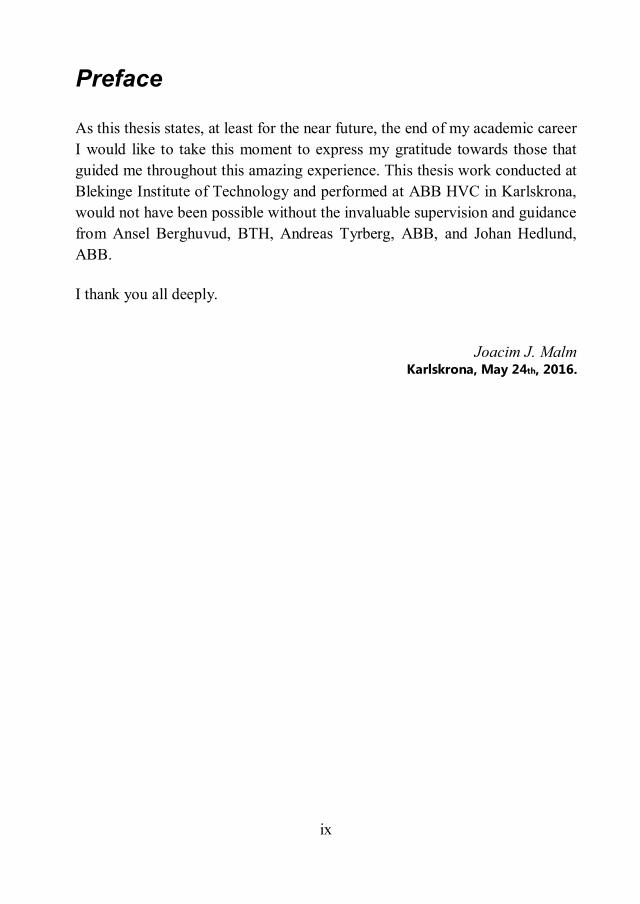
Preface

As this thesis states, at least for the near future, the end of my academic career I would like to take this moment to express my gratitude towards those that guided me throughout this amazing experience. This thesis work conducted at Blekinge Institute of Technology and performed at ABB HVC in Karlskrona, would not have been possible without the invaluable supervision and guidance from Ansel Berghuvud, BTH, Andreas Tyrberg, ABB, and Johan Hedlund, ABB. I thank you all deeply.

Joacim J. Malm Karlskrona, May 24th, 2016.

xi

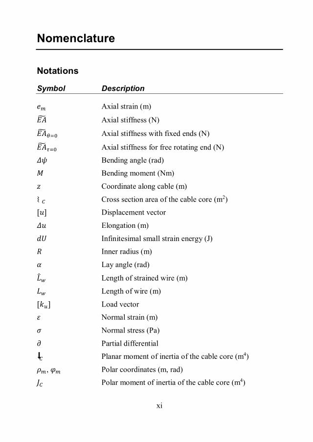
Nomenclature

Notations

Symbol Description

Axial strain (m)

Axial stiffness (N)

Axial stiffness with fixed ends (N)

Axial stiffness for free rotating end (N)

Bending angle (rad)

Bending moment (Nm) Coordinate along cable (m)

⌇ Cross section area of the cable core (m2)

[ ] Displacement vector

Elongation (m)

Infinitesimal small strain energy (J)

Inner radius (m)

Lay angle (rad)

Length of strained wire (m)

Length of wire (m)

[ ] Load vector

Normal strain (m)

Normal stress (Pa)

Partial differential

⬇ Planar moment of inertia of the cable core (m4)

, Polar coordinates (m, rad)

Polar moment of inertia of the cable core (m4)

xii

Pure shear stress (Pa)

Pure shear strain (m) Rotation angle (rad)

⤇ Shear modulus of the cable core (Pa)

Stiffness coefficient for coupled axial torsion

[ ] Stiffness matrix

Tension (N)

Torsional stiffness (Nm2)

Torque (Nm)

Torque tension coupling coefficient

Total number of armour wires in the layer (#)

Total internal strain energy (J)

Twist tension coupling coefficient

Variation of external energy (J)

Variation of external work energy (J)

Variation of virtual work (J)

Variation of the internal strain energy (J)

Young’s modulus for armour wire (Pa)

Young’s modulus for cable core (Pa) ….. …….

Acronym Description

ASEA Allmänna Svenska Elektriska Aktiebolaget

ABB ASEA Brown Boveri Ltd BBC Brown Boveri et Cie

CAS Computer Algebra Calculation XLPE Cross-Linked Polyethylene

xiii

DOF Degrees of Freedom

DoFs Degrees of Freedom System FE Finite Element

HVC High Voltage Cables CWI National Research Institute for Mathematics and

Computer Science MI Paper Lapped

RAOs Response Amplitude Operators ….. …..

xv

Table of Contents

1 INTRODUCTION ................................................................ 1 Background 1

Organization of ABB 1 Problem 1

Problem statement 4 Purpose 4 Delimitations 5

Within coupling between tension and torque 5 Within OrcaFlex 5

2 THEORETICAL FRAMEWORK ...................................... 7 Related research 7 Modelling 8

Coupling between tension and torque 8 Theoretical axial stiffness and simplifications 10

For free rotating end 10 For fixed end 10

Theoretical background for hanging cable 11 Fixed – Fixed boundaries 11 Fixed – Free boundaries 12

3 METHOD ........................................................................... 13 Implementation 13

Programming 13 Python external function 13

Simulation 15 Case 1 – Cable under constant tension 15 Case 2 – Cable under varying tension 16 Case 3 – Free hanging cable with seabed interaction 17

Experimental testing 18 Test 1 19 Test 2 21

4 RESULTS ........................................................................... 23 From analytical model and external function 23

Case 1 - Cable under constant tension 23 Fixed – Fixed boundaries 23 Fixed – Free boundaries 26 Free – Free boundaries 28

xvi

Case 2 - Cable under varying tension 31 Fixed – Fixed boundaries 31 Fixed – Free boundaries 34

Case 3 – Free hanging cable with seabed interaction 36 Fixed – Fixed boundaries 36 Fixed – Free boundaries 39

Analysis of results from experimental test 42 Test 1 42

Simulation of result in Test 1 45 Test 2 46

Simulation of result in Test 2 48

5 DISCUSSION ...................................................................... 51 Discussion of analytical model and external function 51

Case 1 - Cable under constant tension 51 Fixed – Fixed boundaries 51 Fixed – Free boundaries 51 Free – Free boundaries 51

Discussion of hanging cable 52 Case 2 – Cable under varying tension 52 Case 3 - Free hanging cable with seabed interaction 52

Discussion of results from experimental test 53 Test 1 53 Test 2 54

Discussion of results 54 Comparison of results for a cable with constant tension and

one fixed boundary and one free 55 Comparison of results for a cable with constant tension and free boundaries 56

Discussion of methodology 56

6 CONCLUSIONS ................................................................. 57

7 RECOMMENDATIONS AND FUTURE WORK ............ 59

8 REFERENCES ................................................................... 60 Literature 61 Web pages 62

APPENDIX A: DERIVATION OF COUPLING BETWEEN TENSION AND TORQUE

APPENDIX B: DESCRIPTION OF ORCAFLEX

1

1 INTRODUCTION This chapter describes the background, problem statement, purpose and delimitations within the project.

Background Organization of ABB

Through the merging of the Swedish company Allmänna Svenska Elektriska Aktiebolaget (ASEA) and the Swiss company Brown Boveri et Cie (BBC) in 1988, ASEA Brown Boveri Ltd (ABB) was formed. Today this merged company with headquarter in Zürich employs over 155 000 persons in over 100 countries. ABB is today known as one of the global leaders within automatization and power technologies. In Sweden ABB has over 9300 employees at over 30 locations and 800 of these is located at HVC (High Voltage Cables) in Karlskrona. HVC is a subdivision of Power Systems and is manufacturing high voltage cables for both land and sea (ABB, 2016).

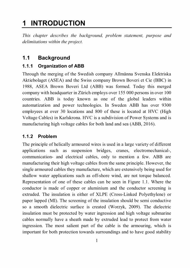
Problem The principle of helically armoured wires is used in a large variety of different applications such as suspension bridges, cranes, electromechanical-, communication- and electrical cables, only to mention a few. ABB are manufacturing their high voltage cables from the same principle. However, the single armoured cables they manufacture, which are extensively being used for shallow water applications such as off-shore wind, are not torque balanced. Representation of one of these cables can be seen in Figure 1.1. Where the conductor is made of copper or aluminium and the conductor screening is extruded. The insulation is either of XLPE (Cross-Linked Polyethylene) or paper lapped (MI). The screening of the insulation should be semi conductive so a smooth dielectric surface is created (Worzyk, 2009). The dielectric insulation must be protected by water ingression and high voltage submarine cables normally have a sheath made by extruded lead to protect from water ingression. The most salient part of the cable is the armouring, which is important for both protection towards surroundings and to have good stability

2

towards tension and torsion. The armouring is often made from galvanized steel wire, but it happens that copper, aluminium or brass also are being used.

Figure 1.1 Representation of a helically single armoured cable, which is not

balanced against torque

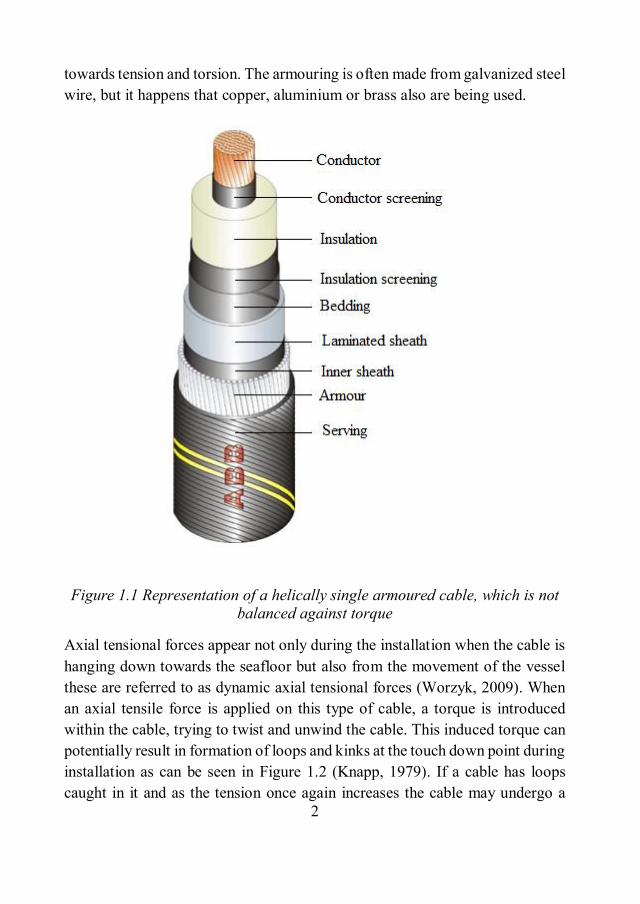
Axial tensional forces appear not only during the installation when the cable is hanging down towards the seafloor but also from the movement of the vessel these are referred to as dynamic axial tensional forces (Worzyk, 2009). When an axial tensile force is applied on this type of cable, a torque is introduced within the cable, trying to twist and unwind the cable. This induced torque can potentially result in formation of loops and kinks at the touch down point during installation as can be seen in Figure 1.2 (Knapp, 1979). If a cable has loops caught in it and as the tension once again increases the cable may undergo a

3

plastic deformation around the loops and this can further lead to an unwanted permanent damage on the cable (Coyne, 1990).

Figure 1.2 Loops and kinks created by induced torque (Perkins, 2016).

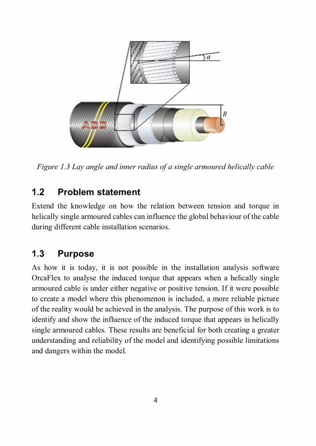
It is also well known that this induced torque has negative consequences on the total strength of the cable (Knapp, 1979). The single helically armoured cable consists of a number of armour wires wrapped around the central core in a helically structure. The constants as seen in Figure 1.3 that defines the structure of the cable is the lay angle ( ) which is the slope of the armour wire applied on the cable and the inner radius ( ) which is the distance from the core centre to the centre of any armour wire in the layer (Lanteigne, 1985).

4

Figure 1.3 Lay angle and inner radius of a single armoured helically cable

Problem statement Extend the knowledge on how the relation between tension and torque in helically single armoured cables can influence the global behaviour of the cable during different cable installation scenarios.

Purpose As how it is today, it is not possible in the installation analysis software OrcaFlex to analyse the induced torque that appears when a helically single armoured cable is under either negative or positive tension. If it were possible to create a model where this phenomenon is included, a more reliable picture of the reality would be achieved in the analysis. The purpose of this work is to identify and show the influence of the induced torque that appears in helically single armoured cables. These results are beneficial for both creating a greater understanding and reliability of the model and identifying possible limitations and dangers within the model.

5

Delimitations Within coupling between tension and torque

The analytical model by Lanteigne does not account for displacement in the radial direction. This displacement is small, compared to the elongation in the length of the cable and has therefore not been considered in the analysis. All armoured wires are also considered to have the same radius and material constants. Within the derivation of the coupling, the conductor is modelled as a homogeneous structure. Calculations will therefore be done for a uniform core with armoured wires wound helically around it.

Within OrcaFlex Delimitations within complex softwares such as OrcaFlex, which is specifically designed to model various structures in dynamic water, is always necessary. It is possible to include many different features in the simulations and it is always a matter of prioritizing. It is possible to include complex phenomena such as nonlinear wave patterns, nonlinear soil models for seabed interactions, different wave and current induced forces, independent motion of vessel, and many more. These more advanced features will not be included in the analysis. However, many of these advanced features will be left for implementation within future research. This is due to both the extra computational cost and that there are not any expectations that these additional features will add any additional value within the data for the analysis. One example that could be included is the seabed friction, which is a highly complex and greatly nonlinear feature. It takes into account things like what deformation of the seabed that would occur if the cable were to be dragged across it. It is also possible to add wind and current induced forces within the simulation. However, these features, as many others will not be included.

7

2 THEORETICAL FRAMEWORK This chapter describes related research within the targeted model and shows the analytical model that will be used for conducting simulations.

Related research It is well known that when a helically single armoured cable is put under an external tension, an internal torque appears that will try to twist the cable. Therefore, any variation in external tension, either negative or positive will induce the cable with a change of torque (Knapp, 1979). There have been many different authors trying to predict the structural response of the cable. The famous work by research scientist Lanteigne (1985) which is widely being cited throughout this report shows a theoretical estimation of the response of helically armoured cables to tension, torsion, and bending. It produces a method to determine the response for helically armoured cables under static loading conditions for both intact cables and when an arbitrary number of constituent wires have failed and will leave the cable unbalanced. It was mainly based on the work of Knapp (1979) which developed a new stiffness matrix for straight helically armoured cables considering tension and torsion. Knapp took into consideration the compression of the central core element, which created internal geometric nonlinearities. The true pioneer in this area though is Hruska (1952) which developed methods for determining the mechanical properties of armoured wire ropes and this method opened up for all following research and literature around this subject. Raoof and Hobbs (1988) proposed a change to the work of Knapp (1979), and instead of considering an aluminium core with steel reinforced cables they chose to use an orthotropic material formulation and view the armour wires as shells. Coyne (1990) did an analysis of the formation and elimination of loops in twisted cables it furthermore investigated what phenomena that would occur when a fast relaxation of a cable that previously had been under an axial tensional load was done quickly.

8

Slippage of the wires in the cables during bending was briefly introduced in the work of Lanteigne but was further developer by Sævik and Gjøsteen (2012) in a strength analysis modelling of flexible umbilical members for marine structures.

Modelling The used model is mainly built upon the previous work of Lanteigne (1985), however Lanteigne (1985) did not show all details regarding the derivation of the established equations. This chapter will follow a similar approach but will show the mathematical steps more clearly and help create a much deeper understanding of the model. Lanteigne (1985) derives the formulation for a number of layers of wires but in this case, the derivation is done for one layer of armour wire.

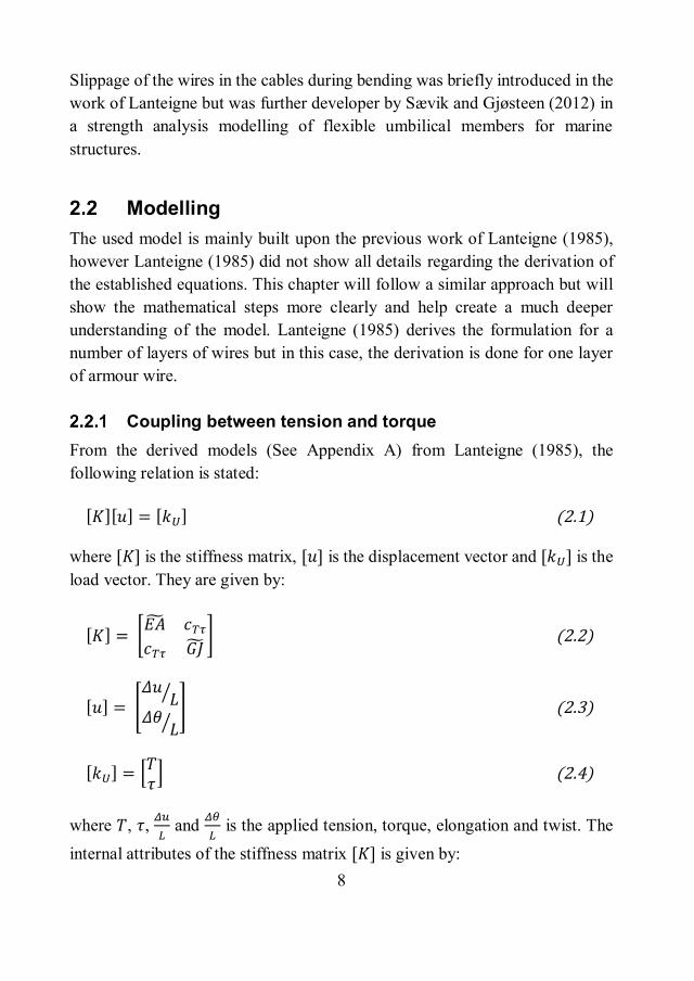
Coupling between tension and torque From the derived models (See Appendix A) from Lanteigne (1985), the following relation is stated:

[ ][ ] = [ ] (2.1) where ] is the stiffness matrix, ] is the displacement vector and ] is the load vector. They are given by:

[ ] = (2.2)

[ ] = (2.3)

[ ] = (2.4)

where , , and is the applied tension, torque, elongation and twist. The internal attributes of the stiffness matrix ] is given by:

9

Axial stiffness:

= ( ) + ⌇ (2.5) where , , ⌇ , and is the cable armouring properties; number of armouring wires, Young's modulus of wire, cross section area of wire and the lay angle of the cables. and ⌇ is the cable core properties; Young's modulus of the core and cross section area of the core. Torsional stiffness:

= ( ) ( ) + ⤇ (2.6) where is the radius from the centre of the core to the centre of the armouring wire core. ⤇ and is the cable core properties; shear modulus of the core and the polar moment of inertia of the core. Stiffness coefficient for coupled axial torsion:

= ( ) ( ) (2.7) By expanding equation 2.1, the coupling between tension and torque is given by:

=

+ ( − ) (2.8)

= + ( − ) (2.9)

where Equation 2.8 is describing torque with relation to tension and elongation and Equation 2.9 is describing torque with relation to tension and radial twist.

10

Theoretical axial stiffness and simplifications For free rotating end

The theoretical axial stiffness at a free rotating end can be calculated by solving Equation 2.1 with zero torque in the boundary, hence using:

= − ) (2.10) where the theoretical axial stiffness at a free rotating end is given by:

= ( ⌇ ( ) ⌇ − ( ) ( ))( ) ( )

) (2.11) Further simplifications can be made for free boundaries, where it is impossible for torque, and this result in the following equation for twist:

(2.12) where is considered the twist tension coupling coefficient and it is calculated as:

= ) (2.13)

For fixed end

The theoretical axial stiffness at a fixed end can be calculated by solving Equation 2.1 with zero rotation in the boundary, hence using:

= ) (2.14) where the theoretical axial stiffness with fixed ends is given by:

= ( ) ⌇ (2.15)

11

Further simplifications can be made for fixed boundaries where it is impossible for radial twist and this result in the following equation for torque:

(2.16) where is considered the torque tension coupling coefficient and it is calculated as:

= (2.17)

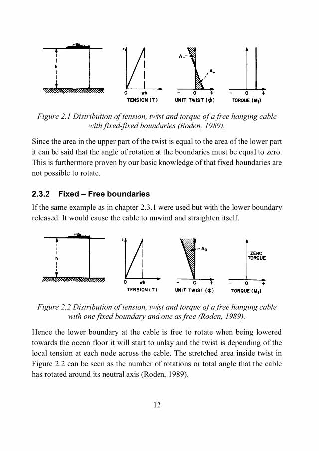
Theoretical background for hanging cable From simple mechanics, Roden (1989) describes the distribution for tension, twist and torque on fixed- free boundaries, and free-free boundaries. Which can be seen in Figure 2.1 and Figure 2.2.

Fixed – Fixed boundaries With the cable-ship still at sea and a part of the cable with a rotational restriction at the boundaries is lowered to the bottom of the sea. The resulting distribution of tension, twist and torque can be seen in Figure 2.1 for fixed – fixed boundaries. The tension is changing linearly along the length of the cable and it is because of the built up in mass. The tensile force creates a torque in the cable and since the cable is prevented from twisting at the ends, an internal torque will be generated at the boundaries. This torque will be constant along the cable (Roden, 1989). The twist that can be seen in Figure 2.1 can best be described by; at the upper part, close to the ship, the cable will try to untwist and straighten the armour resulting in negative twist. At the bottom of the cable where there is not any tension there will not be any untwisting of the armouring, furthermore the elastic nature of the cable will resist untwisting and result in a positive twist. It can be explained better by viewing the cable in two different parts. The part above the half-depth of the cable will untwist and the part below the half-depth will be tightened (Roden, 1989).

12

Figure 2.1 Distribution of tension, twist and torque of a free hanging cable

with fixed-fixed boundaries (Roden, 1989).

Since the area in the upper part of the twist is equal to the area of the lower part it can be said that the angle of rotation at the boundaries must be equal to zero. This is furthermore proven by our basic knowledge of that fixed boundaries are not possible to rotate.

Fixed – Free boundaries If the same example as in chapter 2.3.1 were used but with the lower boundary released. It would cause the cable to unwind and straighten itself.

Figure 2.2 Distribution of tension, twist and torque of a free hanging cable

with one fixed boundary and one as free (Roden, 1989).

Hence the lower boundary at the cable is free to rotate when being lowered towards the ocean floor it will start to unlay and the twist is depending of the local tension at each node across the cable. The stretched area inside twist in Figure 2.2 can be seen as the number of rotations or total angle that the cable has rotated around its neutral axis (Roden, 1989).

13

3 METHOD In this chapter the implementation of the external function will be presented and simulations will be described. Furthermore, the equipment and process for experimental testing will be described.

Implementation Implementation of the coupling between tension and torque within OrcaFlex is done by using an external function that will help to insert the wanted torque at each node on the OrcaFlex model. Further information regarding models within OrcaFlex and environmental influences can be viewed in Appendix B.

Programming Python is a completely open source high level programming language, which was developed by Guido van Rossum at CWI (National Research Institute for Mathematics and Computer Science) in Netherlands between the late eighties and the early nineties. Python resemble many other programming languages such as ABC, C, C++ and UNIX (Python, 2016).

Python external function The external function is a construction of three classes. What the three classes all have in common is that they all are constructed by an initialise part and a calculation part. The initialise part handles the model objects, period, steps and finds where the applied loads are located on the model. The calculation part then uses the gathered information from the initialise part to calculate the value that will be used for each applied load (Python, 2016). The first class is created to be used for the first fixed or free boundary and applies the equation for calculating torque from tension and twist as can be seen in Equation 2.9. What it does is that it identifies which tension and twist that exists at each node and then uses these found values to calculate the torque and then applies this torque to the node. The OrcaFlex model is built up by segments (See Appendix B) and it is the number of created segments that is controlling

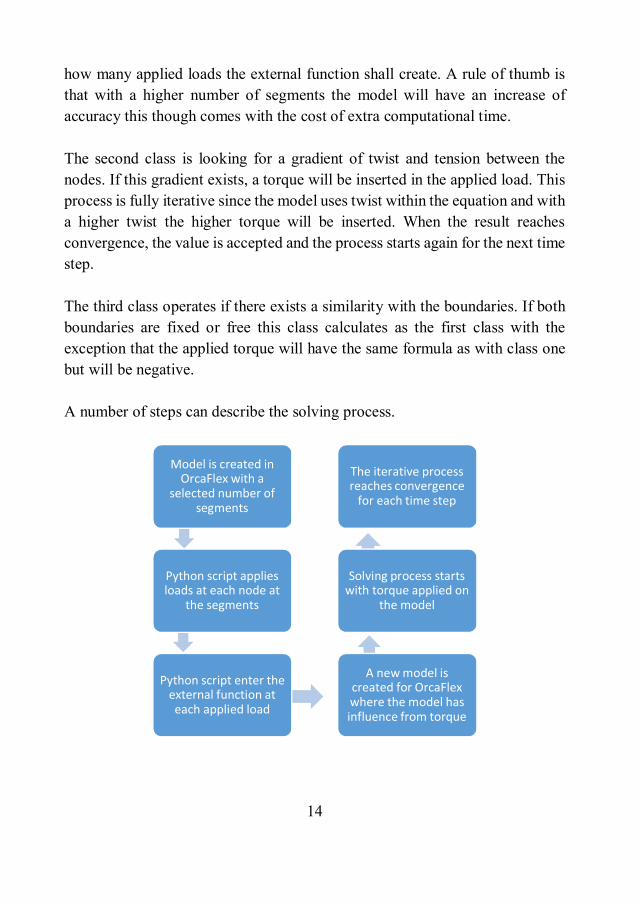
14

how many applied loads the external function shall create. A rule of thumb is that with a higher number of segments the model will have an increase of accuracy this though comes with the cost of extra computational time. The second class is looking for a gradient of twist and tension between the nodes. If this gradient exists, a torque will be inserted in the applied load. This process is fully iterative since the model uses twist within the equation and with a higher twist the higher torque will be inserted. When the result reaches convergence, the value is accepted and the process starts again for the next time step. The third class operates if there exists a similarity with the boundaries. If both boundaries are fixed or free this class calculates as the first class with the exception that the applied torque will have the same formula as with class one but will be negative. A number of steps can describe the solving process.

Model is created in OrcaFlex with a

selected number of segments

Python script applies loads at each node at

the segments

Python script enter the external function at each applied load

A new model is created for OrcaFlex where the model has influence from torque

Solving process starts with torque applied on

the model

The iterative process reaches convergence

for each time step

15

The external function starts at = −10s. This is before the dynamics is applied on the model which is at = 0 this is so the torque can be staggered and that the model will find convergence at each step. This is done mainly because it is preferable to increase the applied torque in a controlled manner rather than applying it all at once. If the torque is applied all at once, it would be seen as an impulse for the simulation and it would introduce unwanted motions (Dingeman, 1997).

Simulation The external function is applied at an arbitrary amount of nodes and this will cause the cable to rotate. If the external function is disabled, no twist will occur. Simulations for three different cases where the first and second case will help to establish the reliability of the created external function and during the third case the dynamic movement, wave pattern and integration with the seabed will be included.

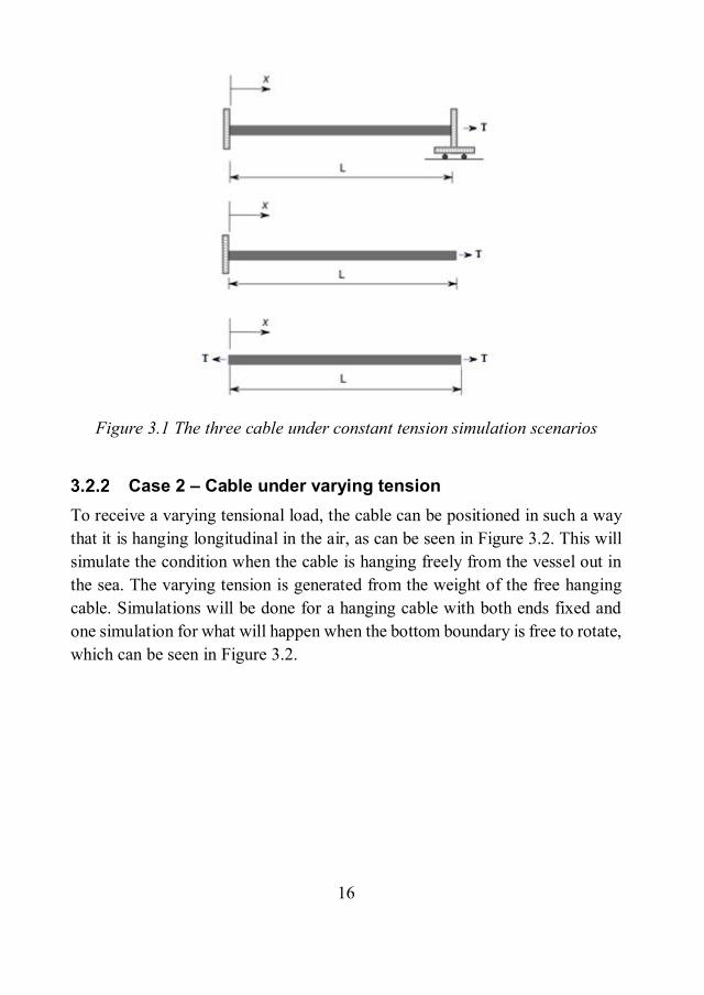
Case 1 – Cable under constant tension A constant force will be applied on the cable and three different pair of boundary conditions will be simulated which can be seen in Figure 3.1. First simulation will show what happens when a cable which is fixed in both boundaries, is pulled with a constant tension. Second simulation will have one fixed boundary and one free, and the third simulation within the cable with constant tension will be for a cable that is fully free to rotate in both boundaries.

16

Figure 3.1 The three cable under constant tension simulation scenarios

Case 2 – Cable under varying tension

To receive a varying tensional load, the cable can be positioned in such a way that it is hanging longitudinal in the air, as can be seen in Figure 3.2. This will simulate the condition when the cable is hanging freely from the vessel out in the sea. The varying tension is generated from the weight of the free hanging cable. Simulations will be done for a hanging cable with both ends fixed and one simulation for what will happen when the bottom boundary is free to rotate, which can be seen in Figure 3.2.

17

Figure 3.2 The two cable under varying tension simulation scenarios

Case 3 – Free hanging cable with seabed interaction

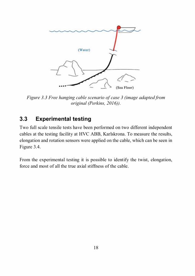
By including the hanging cable which was presented in case two and increasing the length of the cable so it will be in full contact with the seabed. This will give a more realistic observation of a cable installation scenario which can be seen in Figure 3.3. The influence of airy waves and elastic linear seabed model (See Appendix B) will be included in the simulation. Simulations will be done for both when the cable is fixed in both boundaries and when the bottom part can rotate freely as the upper part is fixed.

18

Figure 3.3 Free hanging cable scenario of case 3 (image adapted from

original (Perkins, 2016)).

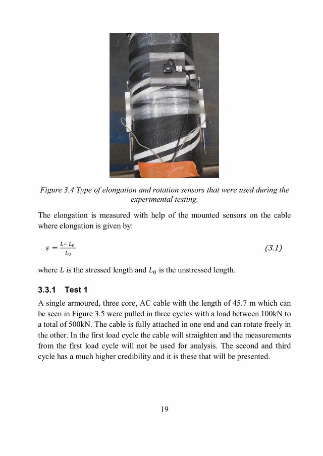
Experimental testing Two full scale tensile tests have been performed on two different independent cables at the testing facility at HVC ABB, Karlskrona. To measure the results, elongation and rotation sensors were applied on the cable, which can be seen in Figure 3.4. From the experimental testing it is possible to identify the twist, elongation, force and most of all the true axial stiffness of the cable.

19

Figure 3.4 Type of elongation and rotation sensors that were used during the experimental testing.

The elongation is measured with help of the mounted sensors on the cable where elongation is given by:

= (3.1) where is the stressed length and is the unstressed length.

Test 1 A single armoured, three core, AC cable with the length of 45.7 m which can be seen in Figure 3.5 were pulled in three cycles with a load between 100kN to a total of 500kN. The cable is fully attached in one end and can rotate freely in the other. In the first load cycle the cable will straighten and the measurements from the first load cycle will not be used for analysis. The second and third cycle has a much higher credibility and it is these that will be presented.

20

Figure 3.5 Single armoured, three core, AC cable and moulding device

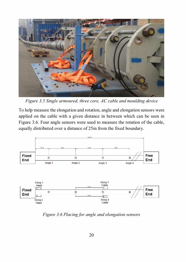
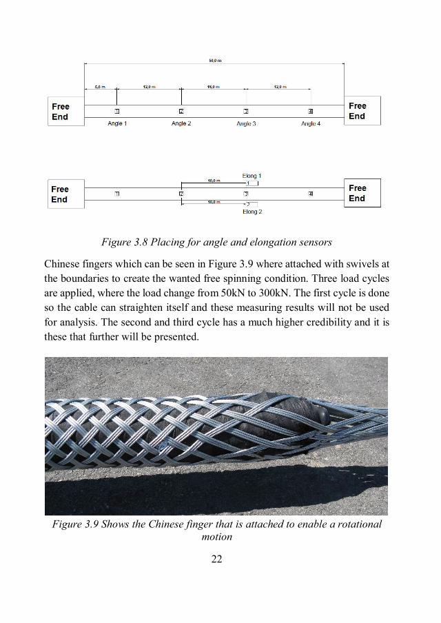
To help measure the elongation and rotation, angle and elongation sensors were applied on the cable with a given distance in between which can be seen in Figure 3.6. Four angle sensors were used to measure the rotation of the cable, equally distributed over a distance of 25m from the fixed boundary.

Figure 3.6 Placing for angle and elongation sensors

21

Test 2 A single armoured DC cable with the length of 50m, which can be seen in Figure 3.7, were pulled with a constant tension of 300kN. The cable can rotate freely in both ends of the cable. To help measure the elongation and rotation, angle and elongation sensors where applied on the cable which can be seen in Figure 3.8.

Figure 3.7 The experimental setup of the tensile test of a single armoured, DC

cable

22

Figure 3.8 Placing for angle and elongation sensors

Chinese fingers which can be seen in Figure 3.9 where attached with swivels at the boundaries to create the wanted free spinning condition. Three load cycles are applied, where the load change from 50kN to 300kN. The first cycle is done so the cable can straighten itself and these measuring results will not be used for analysis. The second and third cycle has a much higher credibility and it is these that further will be presented.

Figure 3.9 Shows the Chinese finger that is attached to enable a rotational

motion

23

4 RESULTS In this chapter the results from the analytical solution will be compared with the computational simulations. Results from the hanging cable will be compared with the known mechanics and furthermore an analysis will be presented on the results from the experimental testing.

From analytical model and external function Data parameters used in the analysis with the numerical model is the data parameters calculated by the analytical model.

Case 1 - Cable under constant tension In the cable under constant tension simulations were performed on a cable with the length of 50m and the constant effective tension for results in chapter 4.1.1.1 and 4.1.1.3 is 300kN and for results in chapter 4.1.1.2 the constant effective tension is set to 400kN.

Fixed – Fixed boundaries From Equation 2.10 it can be calculated and shown that all nodes over the cable with constant tension should have a constant internal torque. The cable should be squeezed tighter and no twist should be possible. A representation of the scenarios is given in the element case of a fixed-fixed beam in Figure 4.1.

24

Figure 4.1 Element case of a helically single armoured cable with both

boundaries fixed

A visual representation of the computational simulation of a fixed – fixed cable can be seen in Figure 4.2. A better view of twist and external torque can be observed in Figures 4.3 and 4.4.

Figure 4.2 Twist and elongation of a cable with fixed ends at a constant

tension of 300kN

From Figure 4.3 it is shown that if there is a constant tension with two fixed ends it will give a twist that will approach zero the more the cable is stretched. The external torque, which can be seen in Figure 4.4 states that the applied

25

torque needs be more frequent at the boundaries because they will try to twist and get loose from the boundaries.

Figure 4.3 Twist of a cable with fixed ends at a constant tension of 300kN

Figure 4.4 External torque on a cable with fixed ends at a constant tension of

300kN

26

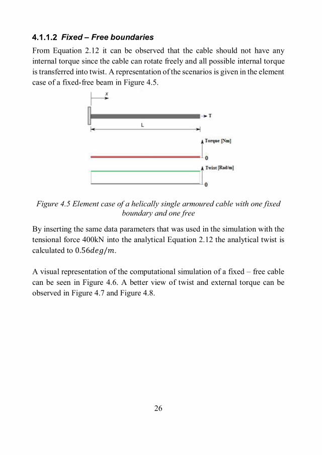
Fixed – Free boundaries From Equation 2.12 it can be observed that the cable should not have any internal torque since the cable can rotate freely and all possible internal torque is transferred into twist. A representation of the scenarios is given in the element case of a fixed-free beam in Figure 4.5.

Figure 4.5 Element case of a helically single armoured cable with one fixed

boundary and one free

By inserting the same data parameters that was used in the simulation with the tensional force 400kN into the analytical Equation 2.12 the analytical twist is calculated to 0.56 . A visual representation of the computational simulation of a fixed – free cable can be seen in Figure 4.6. A better view of twist and external torque can be observed in Figure 4.7 and Figure 4.8.

27

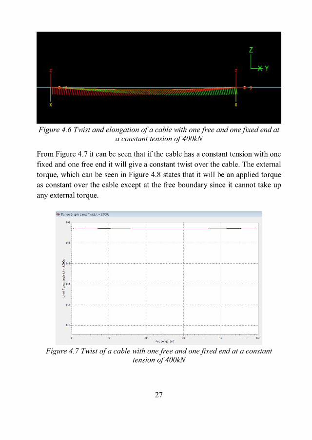
Figure 4.6 Twist and elongation of a cable with one free and one fixed end at

a constant tension of 400kN

From Figure 4.7 it can be seen that if the cable has a constant tension with one fixed and one free end it will give a constant twist over the cable. The external torque, which can be seen in Figure 4.8 states that it will be an applied torque as constant over the cable except at the free boundary since it cannot take up any external torque.

Figure 4.7 Twist of a cable with one free and one fixed end at a constant

tension of 400kN

28

Figure 4.8 External torque on a cable with one free and one fixed end at a

constant tension of 400kN

The computational simulation gives the resulting twist at 400kN of 0.58 which can be seen in Figure 4.7 and the external torque of 8.2 which can be seen in Figure 4.8.

Free – Free boundaries From Equation 2.12 it can be observed that the cable should not have any internal torque since the cable can rotate freely and all possible internal torque is transferred into twist. A representation of the scenarios is given in the element case of a fixed-free beam in Figure 4.9.

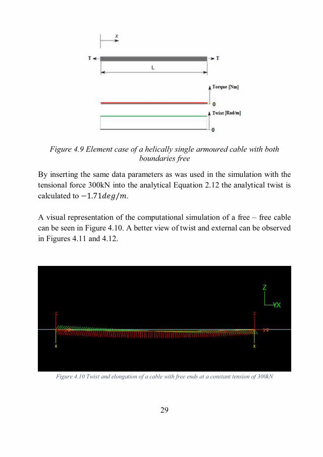
29

Figure 4.9 Element case of a helically single armoured cable with both

boundaries free

By inserting the same data parameters as was used in the simulation with the tensional force 300kN into the analytical Equation 2.12 the analytical twist is calculated to −1.71 / . A visual representation of the computational simulation of a free – free cable can be seen in Figure 4.10. A better view of twist and external can be observed in Figures 4.11 and 4.12.

Figure 4.10 Twist and elongation of a cable with free ends at a constant tension of 300kN

30

If there is a constant tension on a cable with one fixed and one free end it will give a constant twist, which can be seen in Figure 4.11. The external torque, which can be seen in Figure 4.12 states that the applied torque will be constant over the cable except at the free boundaries since a free boundary cannot take up any external torque.

Figure 4.11 Twist of a cable with free ends at a constant tension of 300kN

Figure 4.12 External torque on a cable with free ends at a constant tension of

300kN

31

The computational simulation gives the result for twist at 300kN of −1.65 which can be seen in Figure 4.11 and the external torque of −2.5 which can be seen in Figure 4.12.

Case 2 - Cable under varying tension In the cable under varying tension simulations, a cable with the length of 400m is used and the tensional force is varying from 1900kN to 0kN. The tensional force is exaggerated to further show on the resulting shape of the hanging cable. Since in this case it is only possible to compare with the known shape that is explained further in chapter 2.3: Theoretical background for hanging cable.

Fixed – Fixed boundaries A visual representation of the computational simulation of a hanging fixed – fixed cable can be seen in Figure 4.13. A better view of twist and external torque can be observed in Figure 4.14 and Figure 4.15.

32

Figure 4.13 Twist and rotation of a free hanging cable with fixed ends

If there is a varying tension on a cable with both ends as fixed, it will give a linear twist, which can be seen in Figure 4.14 and the external torque, which can be seen in Figure 4.15 states that the applied torque will be linear over the cable except at the fixed where the external torque will spike.

33

Figure 4.14 Twist of a free hanging cable with fixed ends

Figure 4.15 External torque of a free hanging cable with fixed ends

Since there is a linear twist over the cable, it will give a second order polynomial rotation with absolute maximum of the rotation at the middle of the cable and zero rotation at the boundaries of the cable.

34

Fixed – Free boundaries A visual representation of the computational simulation of a hanging fixed – free cable can be seen in Figure 4.16. A better view of twist and external torque can be observed in Figure 4.17 and Figure 4.18.

Figure 4.16 Twist and rotation of a free hanging cable with one free and one

fixed end

If there is a varying tension on a cable with one fixed end and one free it will give a linear twist which can be seen in Figure 4.17 and the external torque which can be seen in Figure 4.18 states that the applied torque will be linear over the cable.

35

Figure 4.17 Twist of a free hanging cable with one free and one fixed end

Figure 4.18 External torque of a free hanging cable with one free and one

fixed end

Since there is a linear twist over the cable it will give a second order polynomial rotation with absolute maximum of the rotation at the end of the cable and zero rotation at the fixed boundary.

36

Case 3 – Free hanging cable with seabed interaction

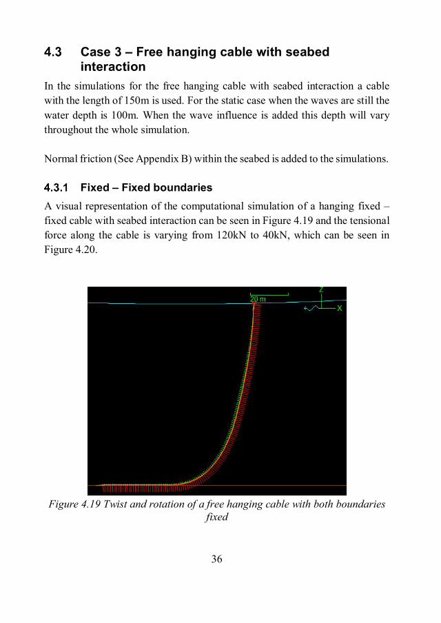
In the simulations for the free hanging cable with seabed interaction a cable with the length of 150m is used. For the static case when the waves are still the water depth is 100m. When the wave influence is added this depth will vary throughout the whole simulation. Normal friction (See Appendix B) within the seabed is added to the simulations.

Fixed – Fixed boundaries A visual representation of the computational simulation of a hanging fixed – fixed cable with seabed interaction can be seen in Figure 4.19 and the tensional force along the cable is varying from 120kN to 40kN, which can be seen in Figure 4.20.

Figure 4.19 Twist and rotation of a free hanging cable with both boundaries

fixed

37

Figure 4.20 Effective tension at the specific arc length of a free hanging cable

with both boundaries fixed

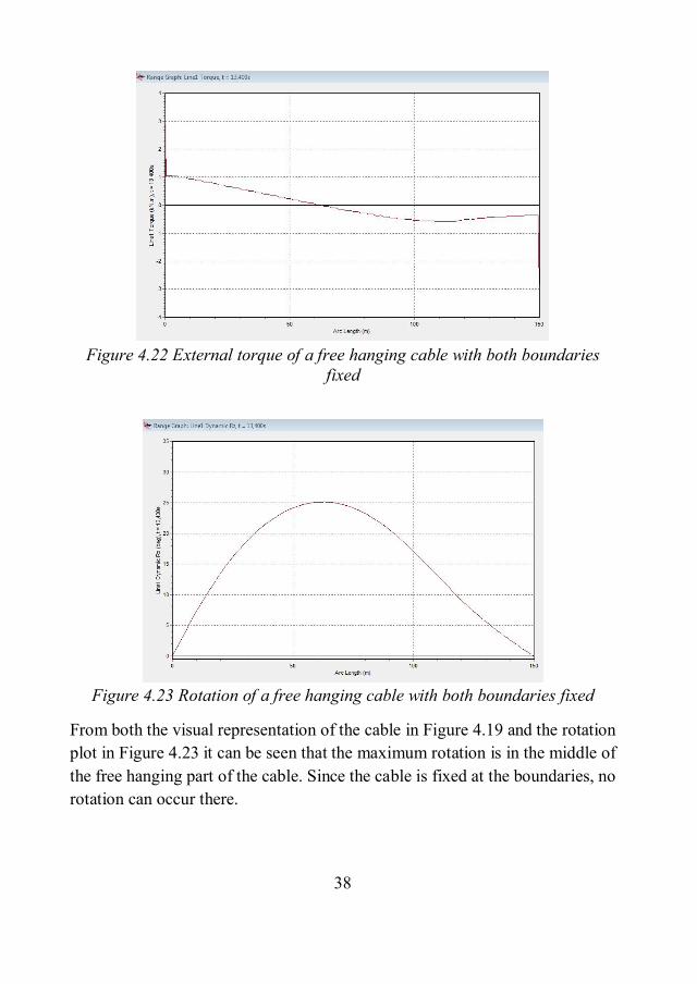
A better view of twist, external torque and rotation of the cable can be observed in Figure 4.21, Figure 4.22 and Figure 4.23.

Figure 4.21 Twist of a free hanging cable with both boundaries fixed

38

Figure 4.22 External torque of a free hanging cable with both boundaries

fixed

Figure 4.23 Rotation of a free hanging cable with both boundaries fixed

From both the visual representation of the cable in Figure 4.19 and the rotation plot in Figure 4.23 it can be seen that the maximum rotation is in the middle of the free hanging part of the cable. Since the cable is fixed at the boundaries, no rotation can occur there.

39

Fixed – Free boundaries A visual representation of the computational simulation of a hanging fixed – free cable with seabed interaction can be seen in Figure 4.24 and the tensional force is varying from 80kN to 0kN which can be seen in Figure 4.25.

Figure 4.24 Twist and rotation of a free hanging cable with one free and one

fixed end

From Figure 4.24 and 4.25 it is also shown that in the valley of the wave the cable will be under compression.

40

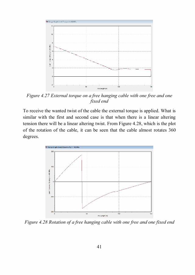
A better view of twist, external torque and rotation of the cable can be observed in Figure 4.35, Figure 4.36 and Figure 4.37.

Figure 4.25 Effective tension at the specific arc length of a free hanging cable

with one boundary fixed and the other one free

Figure 4.26 Twist of a free hanging cable with one free and one fixed end

41

Figure 4.27 External torque on a free hanging cable with one free and one

fixed end

To receive the wanted twist of the cable the external torque is applied. What is similar with the first and second case is that when there is a linear altering tension there will be a linear altering twist. From Figure 4.28, which is the plot of the rotation of the cable, it can be seen that the cable almost rotates 360 degrees.

Figure 4.28 Rotation of a free hanging cable with one free and one fixed end

42

Analysis of results from experimental test Test 1

From the experimental testing of a cable with one end free and the other one as fixed, it can be seen that the smallest rotation is at the fixed boundary and it is increasing linearly towards the free end, which can be seen in Figure 4.29. The rotation is also measured when the cable is fully stretched and when it is under the highest load during the test.

Figure 4.29 Relative rotation at the position of the applied angle sensors

between 100kN and 500kN.

The value at two points from Figure 4.29 is selected independently and divided by the length between them to receive the corresponding twist. In Figure 4.30 this method has been done for five independent pairs.

00,5

11,5

22,5

33,5

4

0 5 10 15 20 25 30

Rota

tion

[deg

]

Length of cable [m]

43

Figure 4.30 Twist from applied angle sensors on the cable between 100kN

and 500kN.

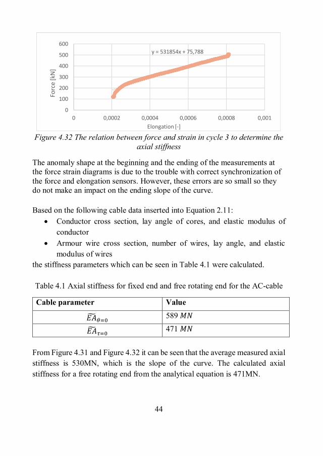
For a cable with constant twist, it also has a linear relation for rotation. In this case, the experimental data shown in Figure 4.29 shows that there cannot be any rotation at the fixed end at the cable and the maximum rotation occurs at the free end of the cable. The elongation is calculated from the known original length and the new stressed length is plotted from cycle two and three in Figure 4.31 and Figure 4.32 against the corresponding pulling force.

Figure 4.31 The relation between force and strain in cycle 2 to determine the

axial stiffness

0

0,05

0,1

0,15

0,2

0,25

0,3

0 1 2 3 4 5 6

Twist

[deg

/m]

Measuring relations [#]

y = 528213x + 66,996

0

100

200

300

400

500

600

0 0,0002 0,0004 0,0006 0,0008 0,001

Forc

e [k

N]

Elongation [-]

44


axial stiffness

The anomaly shape at the beginning and the ending of the measurements at the force strain diagrams is due to the trouble with correct synchronization of the force and elongation sensors. However, these errors are so small so they do not make an impact on the ending slope of the curve. Based on the following cable data inserted into Equation 2.11:

Conductor cross section, lay angle of cores, and elastic modulus of conductor

Armour wire cross section, number of wires, lay angle, and elastic modulus of wires

the stiffness parameters which can be seen in Table 4.1 were calculated. Table 4.1 Axial stiffness for fixed end and free rotating end for the AC-cable

Cable parameter Value

589

471 From Figure 4.31 and Figure 4.32 it can be seen that the average measured axial stiffness is 530MN, which is the slope of the curve. The calculated axial stiffness for a free rotating end from the analytical equation is 471MN.

y = 531854x + 75,788

0

100

200

300

400

500

600

0 0,0002 0,0004 0,0006 0,0008 0,001

Forc

e [k

N]

Elongation [-]

45

Simulation of result in Test 1 Cable parameters that were used in the simulation was calculated based on the analytical Equation 2.11 and can be seen in Table 4.1 and Table 4.2.

Table 4.2 Torsional stiffness and stiffness coefficient for coupled axial torsion for the AC-cable


841850

9.99*106 The experimental results from the fixed-free cable shows the relative rotation from 100kN to 500kN and as the rotation as seen as linear the load for the simulation where 400kN to better simulate the found experimental results. From Figure 4.33 it can be seen that if there is a constant tension on a cable with one fixed and one free end it will give a constant twist of 0.56 over the cable.

Figure 4.33 Twist of a cable with one free and one fixed end at a constant

tension of 400kN

46

Test 2 From the experimental testing of a cable with both ends free the results indicate on a close to linear rotation over the cable which can be seen in Figure 4.34. The smallest rotation is in the middle of the cable and both ends rotate apart from each other. The rotation is also measured when the cable is fully stretched and when it is under the highest load during the test.

Figure 4.34 Relative rotation at the position of the applied angle sensors at

300kN.

The value at two points from Figure 4.34 is selected independently and divided by the length between them to receive the corresponding twist. In Figure 4.35 this method has been done for five independent pairs. The spreading in amplitude between the values in Figure 4.35 indicate that the measuring accuracy could be increased.

Figure 4.35 Twist from applied angle sensors on the cable at 300kN.

-80

-60

-40

-20

0

20

40

60

0 10 20 30 40 50

Rota

tion

[Deg

]

Length of cable [m]

-3,5-3

-2,5-2

-1,5-1

-0,50

0 1 2 3 4 5 6

Twist

[Deg

/m]

Measuring relations [#]

47

For a cable with constant twist it is also having a linear relation for rotation. In this case, the experimental data shown in Figure 4.34 shows that the absolute maximum rotation is biggest at the free boundaries and the middle of the cable have zero rotation. The elongation is calculated from the known original length and the new stressed length and is plotted from cycle two and three in Figure 4.36 and Figure 4.37 against the corresponding pulling force.


axial stiffness


axial stiffness

Based on the following cable data inserted into Equation 2.11: Conductor cross section, lay angle of cores, and elastic modulus of

conductor Armour wire cross section, number of wires, lay angle, and elastic

modulus of wires

y = 420029x - 77,053

0

100

200

300

400

0 0,0002 0,0004 0,0006 0,0008 0,001 0,0012

Forc

e F

[kN

]

Elongation [-]

y = 388517x - 156,76

050

100150200250300350

0 0,0002 0,0004 0,0006 0,0008 0,001 0,0012 0,0014

Forc

e [k

N]

Elongation [-]

48

the stiffness parameters which can be seen in Table 4.3 were calculated. Table 4.3 Axial stiffness for fixed end and free rotating end for the DC-cable


503

386 From Figure 4.36 and Figure 4.37 it can be seen that the average measured axial stiffness is 404MN which is the slope of the curve. The calculated axial stiffness for a free rotating end from the analytical equation is 386MN.

Simulation of result in Test 2 Cable parameters that were used in the simulation was calculated based on the analytical Equation 2.11 and can be seen in Table 4.3 and Table 4.4. Table 4.4 Torsional stiffness and stiffness coefficient for coupled axial torsion

for the DC-cable


88514

-3.26 *106 If there is constant tensional force on a cable with both ends free the simulation results say that it will have a constant twist of −1.65 which can be seen in Figure 4.38

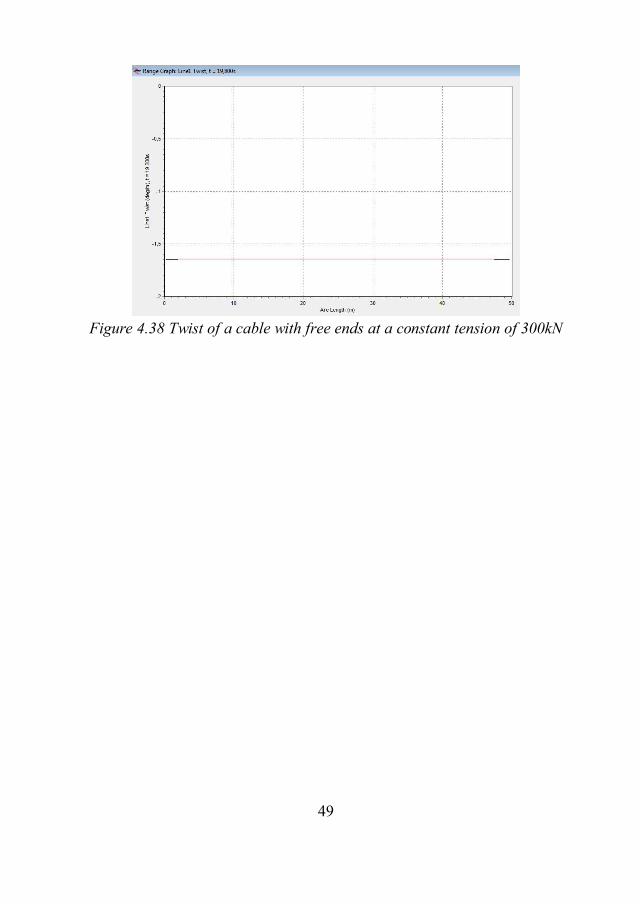
49

Figure 4.38 Twist of a cable with free ends at a constant tension of 300kN

51

5 DISCUSSION In this chapter a discussion of the given results from chapter 4 is found.

Discussion of analytical model and external function

Analytical results compared with the results by implementing the external function.

Case 1 - Cable under constant tension Fixed – Fixed boundaries

By restricting rotation at the boundaries for a cable with constant tension, it will only stretch the cable and no twist will occur. These results are found for both the elementary case and in the simulated case.

Fixed – Free boundaries By using the same cable parameters for both in the simulation and within the analytical calculation it can be seen by doing a straight analytical calculation that the twist will be calculated to 0.56deg/m and compared this to the twist within the simulation that was 0.58deg/m. The difference between these absolute values is 3.5%, which is a considerable accurate value. This strengthens the belief that the external function is correctly implemented within the software.

Free – Free boundaries By using the same cable parameters for both in the simulation and within the analytical calculation it can be seen by doing a straight analytical calculation that the twist will be calculated to -1.71deg/m and compared this to the twist within the simulation that was -1.65deg/m. The difference between these absolute values is 3.6%, which is a good accuracy. This further strengthens the belief that the external function is correctly implemented within the software.

52

Discussion of hanging cable Case 2 – Cable under varying tension

From the research from Roden (1989) which can be viewed in chapter 3.3.2 it shows a clear representation of the wanted shape of torque and twist on the cable. For both the scenarios under case two it is possible to directly compare the results with the elementary case, they all match for the wanted twist, however the simulated torque does not correspond. In these cases, it is not possible to rely on any experimental testing to further validate the method but since the shape of the twist is similar, the method can in the future be altered only by adding a constant to alter the influence of the external torque. It is important to comprehend that the internal net torque must be constant along the length of the hanging cable for when the cable has both boundaries fixed. This is since the rotation of the cable is restricted. For simplification, it can be addressed that if there is any restriction of rotation there will be an internal torque building up, if there on the other hand is not any restrictions there will only be twist.

Case 3 - Free hanging cable with seabed interaction For both scenarios from case three, there is not any earlier study or elementary cases that gives us a solution to compare with accessible. Instead what needs to be done is to compare with the found results in the first and second case and what is possible to conclude is that when the cable has a linear altering tension it also should have a linear twist, and when there is a constant tension on the cable it should have a constant twist. These assumptions and realisations can all be found in the results for both scenarios in case three. Is it sufficient to exclude the computational heavy external function and instead replace it with a single twisting moment at the free boundary of the cable? A simplification to receive the wanted twist is to totally neglect the external function and instead apply a torque at the free boundary that will give the

53

average twist of the cable. This can be suitable when a fast computational calculation is wanted since the usage of the external function greatly increases the time it takes to solve the simulation.

Discussion of results from experimental test Through the experimental testing two different cables where used to validate the analytical and external function. It would have been more beneficial to use the same cable for the two different cases since the exact correlation between the two cables is not known. For future experimental tests, a specific cable could be used to give a better clear picture of the results. The acceleration when stretching the cables was done manually and It would have been beneficial to try to use different accelerations and compare these to see if the acceleration has any influence in the result.

Test 1 From the experimental testing of the cable with one boundary free and the other one free the results state that the twist on the cable is 0.15deg/m and by comparing this with both the computational simulation and analytical calculation, which gave the result 0.56deg/m. The results indicate on a big difference on how free the cable is towards rotation as these results indicate that the free boundary at the experimental testing might not be fully free to rotate. Further, it would have been beneficial to increase the number of angle sensors on the cable to better view the expected linearity of the rotation. However, the simulation and experimental testing is behaving as expected when the rotation is increasing towards the free end of the cable. The analytical axial stiffness for a free rotating AC-cable is calculated to 471MN and from the data from the experimental tests average is calculated to 530MN gives us and relative error of 11%. Which could give us the reason why there is a lower rotation in the analytical solution compared with the experimental. The other explanation is that the free rotating end cannot entirely be seen as a free boundary. This boundary could be more like a semi-free where there still is some twisting restriction. For a cable with fixed ends the analytical

54

axial stiffness is calculated to 589MN which helps further to indicate that the free boundary is more semi-fix since the measured axial stiffness is right in between our calculated axial stiffness for fixed ends and free rotating.

Test 2 From the experimental testing of the cable with both boundaries free the results state that the twist on the cable is -2.7deg/m and by comparing this with both the computational simulation and analytical calculation, which gave the result -1.7deg/m. That gives us an absolute error of 1 degree per meter. The shape of the rotation from simulation and real life testing is similar except from the slope of the rotation. The computational simulation can easily be altered by applying a constant to make it better simulate the reality of the cable. This could be preferable in some cases where it is interesting to know the exact rotation. It is highly interesting that the experimental axial stiffness is calculated to 386MN and the measured from the experimental testing is of an average of 404MN, which is a relative error of 5%. This helps us to further believe in the analytical solution and states that it has a good capacity of estimating the right result for axial stiffness. The measured rotation at 50m on the cable is higher than from the analytical calculations, this conclude that the analytical calculations is underestimating the result.

Discussion of results What is interesting in the results is that the shape of the twist and then the corresponding rotation of the cable match in all scenarios but the torque does not. This is a big insight and it can be explained further by: Since OrcaFlex does not have the built in feature of using a single armoured cable a straight cable is selected, which does not twist when tension is applied. It is possible to simulate the characteristics between tension, torque and twist by applying an external torque on the cable and it will give the wanted twist of the cable. What needs to be stated here is that this applied external torque will not be a

55

representation of the real induced torque that would appear within a single armoured cable. However, the generated twist this applied torque creates, will. The wanted twist is found by applying a torque on the cable at an arbitrary amount of selected nodes. This is however as stated giving us a false torque on the cable. It is for this moment not possible to make the twist and torque to be correct at the same time. This is something that has been found that it cannot be done with the usage of an external function. It somehow needs to be directly implemented into the simulation software.

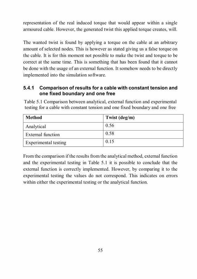
Comparison of results for a cable with constant tension and one fixed boundary and one free

Table 5.1 Comparison between analytical, external function and experimental testing for a cable with constant tension and one fixed boundary and one free

Method Twist (deg/m)

Analytical 0.56

External function 0.58

Experimental testing 0.15 From the comparison if the results from the analytical method, external function and the experimental testing in Table 5.1 it is possible to conclude that the external function is correctly implemented. However, by comparing it to the experimental testing the values do not correspond. This indicates on errors within either the experimental testing or the analytical function.

56

Comparison of results for a cable with constant tension and free boundaries

Table 5.2 Comparison between analytical, external function and experimental testing for a cable with constant tension and one fixed boundary and one free

Method Twist (deg/m)

Analytical -1.71

External function -1.65

Experimental testing -2.7 From the comparison if the results from the analytical method, external function and the experimental testing in Table 5.2 it is possible to conclude that the external function is correctly implemented. However, by comparing it to the experimental testing the values do not correspond. This indicates on errors within either the experimental testing or the analytical function.

Discussion of methodology The usage of an external function within OrcaFlex has limitations. What has been stated before is the fact that with the usage of an external function it is not possible to receive the true internal torque of the cable. This could maybe be done by twisting the cable before doing the simulation and this is functional for static solutions. However, when dynamics is implemented and the tension over the cable is constantly changed over the time interval the twist also should change and this method will fail. What needs to be done is to create a model that will naturally unlay when it is hanging freely. How this is done is outside of the scope of this work and is a good angle for continuing work.

57

6 CONCLUSIONS In this chapter conclusions will be presented over the answer provided for the problem formulation. The problem statement says that the task was to extend the knowledge between tension and torque in helically single armoured cables. Throughout an external function implemented into the simulation software OrcaFlex, the knowledge has greatly extended for typical cable installation scenarios and ordinary cable testing scenarios. After this work, it is possible to identify the real twist and rotation of a given cable for different installation scenarios by introducing an external torque. This external torque is however not always the real internal torque that a tensional stressed helically single armoured cable will induce. The task was to show the influence of the induced torque in the cable, and show how the cable will react from different applied forces, both dynamically and statically. This influence has been shown through three different cases and experimental testing has been done to further validate the results. Through the usage of an external function in OrcaFlex, the big realization has been made that at this moment it is not possible to have the real torque and twist at the same time. A selection needs to be made on which of these aspects that will be targeted. Main problem for this whole scenario is that simulations are made on a single armoured helically cable by twisting a torque balanced cable, which will not induce any torque when tension is applied. The method by using the external function is a good method to find the twist and rotation of the cable.

59

7 RECOMMENDATIONS AND FUTURE WORK

In the future, this created method can be applied on various cable installation scenarios, such as when the cables are pulled to shore, since this leads to great tensional build up inside the cable. However, what is most interesting in that case is the immense torque that the cable is induced with when it is not torque balanced, since the usage of an external function within OrcaFlex cannot show a reliable induced torque some other method needs to be created. Further research by using the external function and applying an external torque on the cable can be done when a correct twist and rotation is of interest. What needs to be stated is that further research needs to be done to fully understand how to implement or identify the induced torque within the cable. One method is to use the found twist and create a cable that naturally twist that amount the first developed method gave in result. What it all comes down to is that it would be beneficial to try to create a more realistic cable that would truly rotate when it is hanging freely. This is something that cannot be done with the usage of an external function and is something that OrcaFlex needs to implement directly into their software. To further try to validate the results in the experimental test 1, where the assumption was that the free boundary was not entirely free towards rotation a model could be created with the usage of OrcaFlex. This model should have a semi-fix boundary to see if it better matches the found axial stiffness from test 1 in the experimental testing.

61

8 REFERENCES

Literature

Coyne, J. (1990) “Analysis of the Formation and Elimination of Loops in Twisted Cables,” IEEE Journal of Oceanic Engineering, vol. 15, no. 2, pp. 72-83. Cribbs, A. (2010) “Model Analysis of a Mooring System for an Ocean Current Turbine Testing Platform”, The College of Engineering and Computer Science. Dingeman, M. W. (1997) “Water Wave Propogation Over Uneven Bottoms”, Advances Series on Ocean Engineering, vol 13, pp.171-184. DNV (Det Norske Veritas, 2007) “Environmental Conditions and Environmental Loads”, DNV-RP-C205. Drazin, P. G. (1977) “On the stability of Cnoidal waves”, Quarterly Journal of Mechanics and Applied Mathematics, vol 30, pp.91-105. Gavin, H. P. (2015) “Strain Energy in Linear Elastic Solids”, Uncertainty, Design and Optimization, Department of Civil and Environmental Engineering. Hjaji, M. A., Mohareb, M. (2013) “Harmonic Response of Doubly Symmetric Thin-walled Members based on the Vlasov Theory”, Department of Mechanical and Industrial Engineering, Tripoli University. Hruska, F. H. (1952) “Radial Forces in Wire Ropes,” Wire Wire Prod, vol 27, pp 459-463. Karegar, S. (2013) “Flexible Risers Global Analysis for Very Shallow Water”, Faculty of Science and Technology. Knapp, R. H. “Derivation of a new stiffness matrix for helically armoured cables considering tension and torsion,” International Journal for Numerical Methods in Engineering, vol. 14, no. 4, pp. 515–529, 1979.

Langhaar, H. L. (1989) “Principles of Virtual Work and Stationary Potential Energy”, Strain Energy Methods in Applied Mechanics, pp.214-223. Lanteigne, J. (1985) “Theoretical Estimation of the Response of Helically Armored Cables to Tension, Torsion, and Bending,” Journal of Applied Mechanics, vol 52, pp. 423–432.

Rerkins, N. (2011) “Thesis Report on Dynamic Fatigue Loads on Composite Downlines in Offshore Service”, Airborne Oil & Gas.

62

Rabe, P. P. (2015) “Thesis Report on Dynamic Fatigue Loads on Composite Downlines in Offshore Service”, Airborne Oil & Gas. Raoof, M., Hobbs, R. E. (1988) “Analysis of multi-layered structural strands,” Journal of Engineering Mechanics, vol 114, no. 7, pp. 1166-1182. Ragab, A-R., Bayoumi, S. E. A. (1998) “Fundamentals and Applications”, Engineering Solid Mechanics, pp.270-271.

Roden, C. E. (1989) “Submarine Cable Mechanics and Recommended Laying Procedures”, pp.103-106.

Sævik, S., Gjøsteen, Ø. J. K. (2012) Strength Analysis Modelling of Flexible Umbilical Members for Marina Structures, Department of Marine Technology. Søreide, T. H. (1986) “Collapse Analysis of Framed Offshore Structures”, The Norwegian Institute of Technology.

Worzyk, T. (2009) “Design, Installation, Repair and Environmental Aspects,” Submarine Power Cables, pp. 27-50.

Web pages ABB., Kort om ABB. Retrieved from: http://new.abb.com/se/om-abb/kort [18 February 2016] ABB., Från Asea till ABB. Retrieved from: http://www.abb.se/cawp/seabb361/dd5ce102d6e2635ac1256b880042aee5.apx [18 February 2016] Orcina., Seabed theory. Retrieved from: http://www.orcina.com [2 Mars 2016] Perkins, N. “cable.jpg”. Retrieved from: http://esciencecommons.blogspot.com/2011/01/undersea-cables-add-twist-to-dna-study.html [2 Mars 2016] Python., Python Overview. Retrieved from: http://www.tutorialspoint.com/python/python_overview.htm [22 February 2016]

63

APPENDIX A: DERIVATION OF COUPLING BETWEEN TENSION AND TORQUE

A.1 Determination of axial strain in wire

Figure A.1 Strain of an arbitrary selected wire m

We know that the axial strain which can be seen in Figure A.1 is given by:

= (A.1) We also see from Figure A.1 that the following connections exist:

= ( )

(A.2)

64

= ( + ) + ( + ( )) (A.3) where is derived using the Pythagoras theorem and using simple trigonometry. Using Equation A.2 and A.3 with Equation A.1 the axial strain of the m:th wire becomes:

= (1 + ) ( ) + ( ( ) + ( )) − 1 (A.4) A simplification is done by linearizing Equation A.4 by neglecting the influence of the second order binomial strain expansions. Hence using the relations,

1 +Δ

= 2Δ

and

( ( )Δ

+ ( )) = 2 ( ) ( )Δ

leads to the equation,

+ 1 = 2 ( ) + 2 ( ) ( ) (A.5) By further expanding left hand side of Equation A.5 and using the relation, (1 + ) = 2 We arrive at the following equation for calculating linear axial strain:

= ( ) + ( ) ( ) (A.6)

65

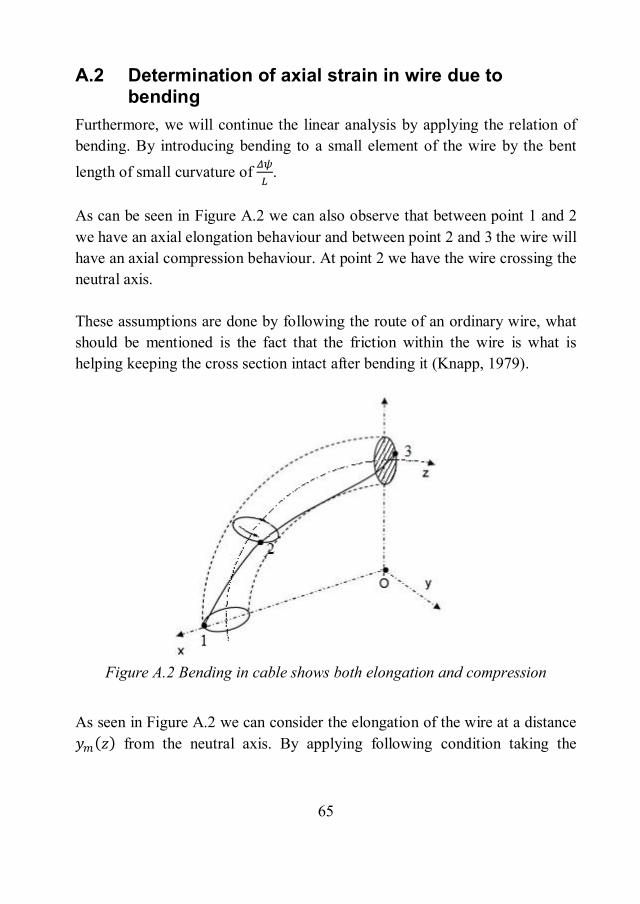
A.2 Determination of axial strain in wire due to bending

Furthermore, we will continue the linear analysis by applying the relation of bending. By introducing bending to a small element of the wire by the bent length of small curvature of . As can be seen in Figure A.2 we can also observe that between point 1 and 2 we have an axial elongation behaviour and between point 2 and 3 the wire will have an axial compression behaviour. At point 2 we have the wire crossing the neutral axis. These assumptions are done by following the route of an ordinary wire, what should be mentioned is the fact that the friction within the wire is what is helping keeping the cross section intact after bending it (Knapp, 1979).

Figure A.2 Bending in cable shows both elongation and compression

As seen in Figure A.2 we can consider the elongation of the wire at a distance

( ) from the neutral axis. By applying following condition taking the

66

banding into account and expanding the axial strain, hence = + ( ) Equation A.6 it can be rewritten into:

= ( ) + ( ) ( ) + ( ) ( ) (A.7) This equation is not balanced towards the neutral axis. We need to define how the equation changes due to varying position of z. This is done by finding an expression for the height of the position of the wire and then adding the influence of z. First we consider the equation to be able to function for any wire around the cable.

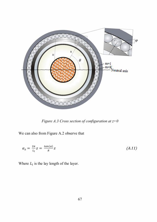
⨇ (0) = ( )) + ( ) (A.8) As can be seen in Figure A.3 we have the following relations 0 ≤ ≤ , 0 ≤ ≤ 2 , and

= (A.9) and where K is the total number of wires in the layer Then we also need to add the relation of increment of position z so that we can have a mean axial strain of the m:th wire in the layer.

⨇ ( ) = ( + ) + ( ) (A.10)

67

Figure A.3 Cross section of configuration at z=0

We can also from Figure A.2 observe that

= = ( ) (A.11) Where is the lay length of the layer.

68

Combine the Equation A.10 and A.11 by letting ( ) = ⨇ ( ) inserting in Equation A.7 we can have a formulation for describing the mean axial strain of the wires. Hence,

= ( ) + ( ) ( )

+ ( ) + ( ) + ( ) (A.12) This equation is giving the axial strain of the m:th wire in the layer of a cable. Where the equation has an axial deformation, rotational strain and curvature part of the wire.

A.3 Energy methods We know from the first law of thermodynamics also known as the law of conservation of energy that: “energy cannot be created or destroyed in a chemical reaction”. What this means is that energy can neither be destroyed nor created. It can only be changed or transferred from one form to another. The internal strain energy, which is created when a system is put under load, will be the same as the external potential energy hence; For elastic materials, we have the principle of minimum potential energy and it follows directly from the principle of virtual work. It defines as,

= + (A.13)

Where is the variation of the internal strain energy and defines as the variation of the external work energy of the applied or external loads as − so we have the following equation for minimum potential energy:

= − (A.14) If we consider the external loads as conservative, excluding for example any frictional manner within the system we have that the overall total potential energy should be equal to zero. Hence:

69

= (A.15) This states that the internal strain energy is equal to the external work energy when no energy losses occur (Ragab and Bayoumi, 1998). Furthermore, if the loads are removed the created strain energy will restore the body to its original structure if the material still is within the elastic region. If the material exceeds this region and crosses the point of yield the material will start to plasticise and will not go back to its original structure (Sævik and Gjøsteen, 2012).

A.3.1 Benefits with energy based derivations If we have a conservative structural system, there are numerous benefits of making the system energy based. Since energy based derivations is mainly using differentiation this method is straightforward and it is less likely to get errors prone to the operation. If we have a more complicated energy gradient derivation a computer program such as CAS can be used to reduce the possibility of making errors in the calculation process. Energy based derivations is not depending on the selection of coordinate system due to the invariance properties of the simplified transformation of residual equations. If the coordinates were to change, we can simply change the DOF in the partial derivatives. Since we performed the linearization, the tangent stiffness matrix is guaranteed to be symmetric. This is seen as an advantage for example when investigating eigenvalues One major concern when solving with energy based derivations is the loss of stability of the system but this can have helped by introducing the singular stiffness criterion. If we have a non-conservative system, we might have to perform a dynamic criterion test which can increase the stability but with the cost of extra computational effort.

70

A.3.1.1 Internal strain energy Consider a small cubic element in the wire, which carries a set of loads as shown below in Figure A.4.

Figure A.4 A small cubic element with a set of loads applied on it

If we consider d to be the infinitesimal small strain energy of this small cubic element it can be written as, (Gavin, 2015):

= +

+ + (A.16)

where , , and is the normal stress, normal strain, pure shear stress and pure shear strain. By integrating the infinitesimal small strain energy over the volume the total strain energy becomes:

= ∫ + + (A.17) By rewriting the number of stresses and strains into vectors we have:

= ∫ { } { } (A.18) Expanding stresses further with Equation A.19 known as the Hook’s law,

71

= (A.19)

The total internal strain energy is then given by:

= ∫ { } { } (A.20) Where the total internal strain energy is bounded by both strain energies from the cable core and the sum of all wires in the layer.

= + ∑ (A.21) By controlling the change of displacements of the wires by (. . ) the variation of the internal strain energy of the wires can be written as:

= + ∑ (A.22) where, [12],

= ∫ { } { } (A.23) where is the volume of element

( )

and can be rewritten as,

=( ) ∫ ∫ { } { } (A.24)

where { } is the axial strain increment for The variation of the internal strain energy of the cable core is given by combining the applied loads, (Søride, 1989):

, = ⌇ ∫ ( ) (A.25)

72

, = ⤇ ∫ ( ) (A.26)

,Ἄ = ⬇ ∫ Ἄ Ἄ (A.27) where , , , , and ,Ἄ , Ἄ is the variation of the internal strain energy and strain due to axial deformation, rotational strain and flexion. The specific strain values can be written as:

= (A.28)

= (A.29)

Ἄ = (A.30) By solving the integration, the formulation for the total variation of the internal strain energy in the cable core is given by, (Hjaji and Mohareb, 2013):

= ⌇ + ⤇ + ⬇ (A.31) Where is the Young’s modulus, ⌇ is the cross section area, is the polar moments of inertia, ⤇ is the shear modulus and ⬇ is the planar moments of inertia, of the cable core. By substituting Equation A.12 into Equation A.24 and solving it, and including Equation A.31 the internal strain energy variation for number of wires for Equation A.22 the solution is given by, (Lanteigne, 1985):

= ⌇ + ⤇ + ⬇

+ ( ( ) + ( ) ( ) + )

73

+ ( ( ) ( ) + ( ) ( )

+ ( ) )

+ ( + ( )

+ + ( + 2 )

2( )

(A.32) Where the constants and are as follows:

= ( )( )

− + ( ) (A.33)

= ( )( )

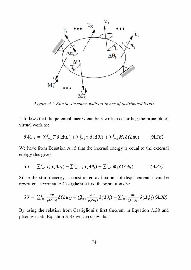
− + ( ) (A.34) A.3.1.2 External stationary potential energy We consider the elastic structure of the cable which are under the influence of a set of distributed and in some cases discrete loads which can be seen in Figure A.5. The stationary potential energy is equal to zero gives:

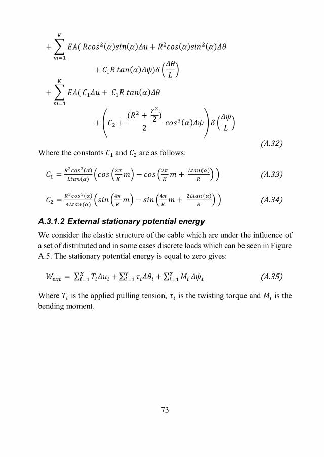
= ∑ + ∑ + ∑ (A.35) Where is the applied pulling tension, is the twisting torque and is the bending moment.

74

Figure A.5 Elastic structure with influence of distributed loads

It follows that the potential energy can be rewritten according the principle of virtual work as:

= ∑ ( ) + ∑ ( ) + ∑ ( ) (A.36) We have from Equation A.15 that the internal energy is equal to the external energy this gives:

= ∑ ( ) + ∑ ( ) + ∑ ( ) (A.37) Since the strain energy is constructed as function of displacement it can be rewritten according to Castiglioni’s first theorem, it gives:

= ∑ℌ( )

( ) + ∑ℌ( )

( ) + ∑ℌ( )

( )(A.38) By using the relation from Castiglioni’s first theorem in Equation A.38 and placing it into Equation A.35 we can show that

75

∑ (ℌ( )

− ) ( ) + ∑ (ℌ( )

− ) ( ) + ∑ (ℌ( )

−) ( ) = 0 (A.39)

This relation from Equation A.39 can only be satisfied for all possible axial deformations, rotational strains and flexion if:

ℌ( )

= (A.40)

ℌ( )= (A.41)

ℌ( )= (A.42)

Furthermore, if we consider only to have = 1, = 1 and = 1 number of influencing loads we have the internal strain energy from external stationary potential energy to be, (Langhaar, 1989):

= ( ) + ( ) + ( ) (A.43)

A.4 Coupling between tension and torque By setting the internal strain energy variation from Equation A.32 equal to the derived internal strain energy variation trough the external stationary potential energy Equation A.43 we have obtained the following relation:

[ ][ ] = [ ] (A.44) where [ ] is the stiffness matrix, [ ] is the displacement vector and [ ] is the load vector. They are given by:

[ ] = (A.45)

[ ] = (A.46)

76

[ ] = (A.47)

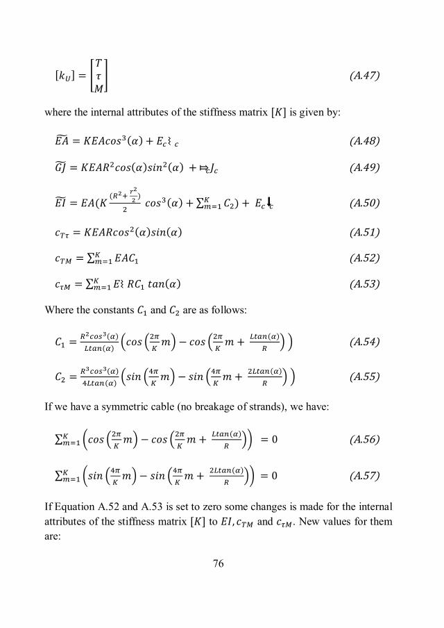
where the internal attributes of the stiffness matrix [ ] is given by:

= ( ) + ⌇ (A.48)

= ( ) ( ) + ⤇ (A.49)

= (( )

( ) + ∑ ) + ⬇ (A.50)

= ( ) ( ) (A.51)

= ∑ (A.52)

= ∑ ⌇ ( ) (A.53) Where the constants and are as follows:

= ( )( )

− + ( ) (A.54)

= ( )( )

− + ( ) (A.55) If we have a symmetric cable (no breakage of strands), we have:

∑ − + ( ) = 0 (A.56)

∑ − + ( ) = 0 (A.57) If Equation A.52 and A.53 is set to zero some changes is made for the internal attributes of the stiffness matrix [ ] to , and . New values for them are:

77

=( )

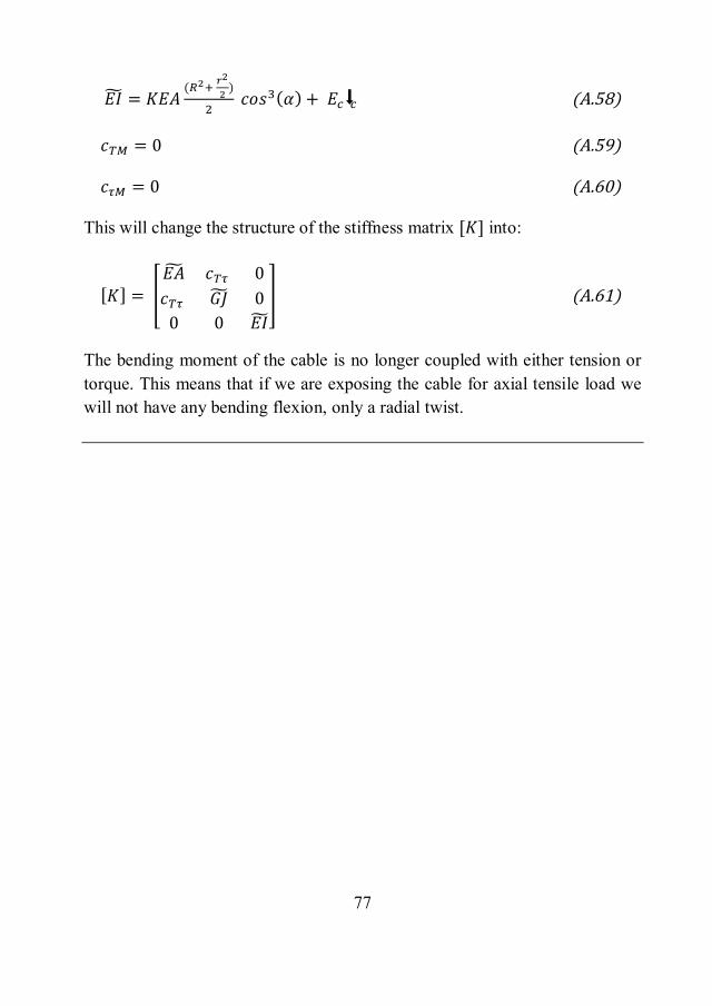
( ) + ⬇ (A.58)

= 0 (A.59)

= 0 (A.60) This will change the structure of the stiffness matrix [ ] into:

[ ] = 0

00 0

(A.61)

The bending moment of the cable is no longer coupled with either tension or torque. This means that if we are exposing the cable for axial tensile load we will not have any bending flexion, only a radial twist.

78

APPENDIX B: DESCRIPTION OF ORCAFLEX

B.1 Description of system OrcaFlex is a finite element software programs capable of solving 3D non-linear arbitrarily deflections. It is specifically designed to be used for doing static and dynamic analysis on marine and offshore structures. OrcaFlex can be used to solve numerous complex problems however the usual problem as with any engineering tool applies that if the operator is inexperienced seemingly correct results can be achieved even though the carried out analysis is badly constructed. However, under the usage of a skilful operator OrcaFlex can be used to create any type of offshore structure from lumped mass elements. From Figure B.1 we can observe the OrcaFlex line model that shows that the weight, mass and buoyancy are lumped to the nodes. The torsion and axial properties of the segments in the actual pipe are expressed as straight rods that are attached to a node at each end. Each node in the discretised model is expressed by combining two half segments, this is always the case with an exception of the nodes at the boundaries.

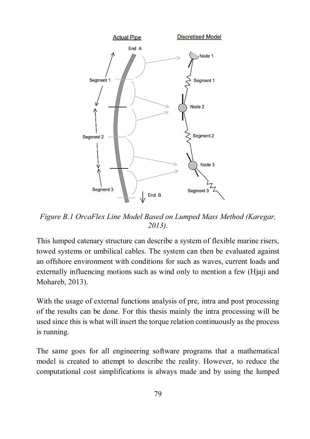
79

Figure B.1 OrcaFlex Line Model Based on Lumped Mass Method (Karegar, 2013).

This lumped catenary structure can describe a system of flexible marine risers, towed systems or umbilical cables. The system can then be evaluated against an offshore environment with conditions for such as waves, current loads and externally influencing motions such as wind only to mention a few (Hjaji and Mohareb, 2013). With the usage of external functions analysis of pre, intra and post processing of the results can be done. For this thesis mainly the intra processing will be used since this is what will insert the torque relation continuously as the process is running. The same goes for all engineering software programs that a mathematical model is created to attempt to describe the reality. However, to reduce the computational cost simplifications is always made and by using the lumped

80

mass approach OrcaFlex can noticeably reduce the computational cost of the mathematical calculations.

B.2 Numerical calculations B.2.1 Statics in OrcaFlex Before a proper dynamic analysis of the structure can be done the static calculation part must be done. This is done to determine the expected shape of the structure and the static equilibrium for each line and buoy element. The static solution can be calculated with the use of the quick method, catenary method or even a specific line shape. However, the most commonly used method is the catenary and it can calculate both hydrostatic and hydrodynamic forces such as: gravity, friction due to seabed, buoyancy, drag from wind or current and axial elasticity. To reach static equilibrium OrcaFlex perform a series of iterative steps:

1. At the start of the process the coordinates for the buoys and vessels

will be calculated by the given data, also a free hanging configuration is calculated for each line according to the specific model.

This first step of the process is important for further calculations since it uses a FE model to determine forces, moments and movements and this FE model is depending on correct coordinates for calculating deviations.

2. Calculate the static equilibrium for each line. To do this the line ends

should be set as fixed. Out of balance forces on each line will be determined.

The second step will estimate a new position for the entire body when determining the out of balance forces.

3. Iterate the first and second step until out of balance forces converge within specified tolerance range.

81

However, these static solutions neglect the influence of bending stiffness and rotational stiffness but since this is only for the static equilibrium it still can be seen as sufficient. B.2.2 Dynamics in OrcaFlex After the static equilibrium is reached, the next stage is to solve the dynamic part. Which is created by time simulations for predetermined time increments. This implies that solutions for external forces that are depending on time can be achieved. The principal difference between the static and dynamic part is that OrcaFlex introduces the Newton’s equation of motion for the dynamic part and it is given by:

( , ) + ( , ) + ( ) = ( , , ) (B.1) where ( , ), ( , ), ( ) and ( , , ) is the system inertia load, system damping load, system stiffness load, and the external load. The depending variables , , and is stated as position, acceleration, velocity, and time. In the beginning of the dynamic solution, the orientation of all objects and their initial position will be collected from the static solution to solve the influencing moment and forces for each object and it can be solved using either the explicit integration scheme or the implicit integration scheme. Whereas the explicit integration scheme solves the simulation using the forward Euler integration with a constant time step to get the acceleration at each node. The solution at the end of each time increment are given by:

( + ) = ( ) + ( ) (B.2)

( + ) = ( ) + ( ) (B.3) where is the time increment. This process is then repeated for each time increment until all nodes are again known.

82

The explicit integration scheme generally takes a longer time to solve since it involves very short time increments. However, for the implicit integration scheme OrcaFlex uses a Generalised- integration scheme which is an iterative solution process that solves the equation of motion at the end of each time increment. Generally, the implicit scheme is stable for a bigger time increment, hence it often means that the implicit scheme solves faster. This can though be a problem for simulations that have a very high non linearity for example an impact simulation (Cribbs, 2010).

B.3 Global analyses B.3.1 Finite element modelling The modelling of the cable will be done using line type elements. Parameters that will be included are:

Outer diameter of the cable [ ] Mass per unit length [ / ] Bending and torsional stiffness [ ] Axial stiffness [ ]

B.3.2 Motion of vessels The motion of the vessels in OrcaFlex is controlled by RAOs (Response Amplitude Operators) which relates the movement of the vessel to the exposing waves. The depending variables for the RAOs is the size and mass of the vessels, and size and periodicity of the waves. The motion of the RAOs, which can be seen in Figure B.2, can be split into two categories; rotation and translation. Where the rotationally part is controlled by pitch, yaw and roll, and translation is controlled by sway, surge and heave. Where the roll, pitch and heave motion generally is considered the most important parameters.

83

Figure B.2 Positive motion as rotation and translation for the six DOF for the

vessel (Cribbs, 2010).

The displacement of the RAOs is defined in vectors such as amplitude and phase. Where the phase vector is defined as the relation between the wave and the motion of the vessel. The amplitude vector is defined as the relation between the amplitude of the wave and the amplitude of the motion of the vessel (Cribbs, 2010).

B.3.3 Modelling environment B.3.3.1 Wave models OrcaFlex has a variation of both regular and irregular wave patterns to use. Regular wave patterns that exists are the Cnoidal, Stokes 5th order and Airy Waves, which can all be seen in Figure B.3.

84

Figure B.3 Regular wave patterns that exists in OrcaFlex

The Cnoidal wave pattern is best suited for shallow water and want to model long waves. It is a periodic wave pattern, which generally has a sharp crest with long wide troughs. This wave pattern is preferable to use when the ratio between the depth and wave length is less than 1/8 (Karegar, 2013). The equation for Cnoidal wave pattern is given by, (Drazin, 1977):

( ) + ⨇ (2 ( ) ) (B.4) where is the horizontal surface elevation depending on position and time , is the trough elevation, ⨇ is the wave height, is the phase speed, is the

wavelength, is the one of the selected Jacobi elliptic functions and ) is the complete elliptic integral of the first kind depending on the shape of the cnoidal wave. The Stokes wave pattern is best suited for when we have and want to model in deep or intermediate waters. A regular nonlinear wave has a lower steepness and smoother crest compared to the Cnoidal wave. This wave pattern is preferable to use when the ratio between the depth and wave length is greater

85

than 1/8 (Karegar, 2013). The equation for Stokes wave pattern is given by, (Dingeman, 1997):

( , ) = ( ( − ) + (2( − )) (B.5) where

= ℎ ( ) (B.6)

= (B.7) The Airy wave pattern, which is the simplest of the three regular wave patterns, is a first order sinusoidal linear wave. It mainly consists of one frequency component to describe the motion of the sinusoidal wave. This pattern is preferable if a small influence of the wave pattern is wanted and if we have deep waters and small waves (Karegar 2013). The equation for Airy wave pattern is given by:

( , ) = ( − ) (B.8) Sometimes the regular wave patterns are not sufficient for describing the model, in those cases a more accurate description of the sea surface is generated by finding the solution of a Fourier series analysis of sinusoidal waves. The wave can be made periodic if we repeat a considered limited time then we have a periodic motion with the given period (Rabe, 2015). Some of these more accurate descriptions are the irregular wave patterns Ochi-Hubble, ISSC and JONSWAP. Irregular waves are used mainly to take into account the big variation of waves in the wave spectrum. It gives the possibility to include the static benefit of waves of different sizes and it helps avoid resonance phenomena that can appear with the usage of regular wave patterns. If we look into the wave spectrum, which is the distribution of energy as a function of frequency for these patterns, we see that the energy within these harmonic waves is proportional to the squared amplitude. A plot of frequency versus energy can therefore show a random wave. An example of this plot can

86

be seen in Figure B.4 where we can see in which frequencies the most wave energy is concentrated and where there does not exist any wave energy (Karegar, 2013).

Figure B.4 Spectral shapes and their corresponding time histories (Rabe,

2015).

By doing extensive analysing of the physical process of old wave records there has been many wave spectra of algebraic form developed. However, the most famous among these wave spectra is a modified version of the Pierson – Moskowits wave spectrum known as JONSWAP which has been developed for the North Atlantic. The mayor difference between them is that over time there is a difference of the growth of the peak wave height. The formulas are given by, (DNV, 2007):

( ) = ⌇ ( ) ( . ) (B.9)

87

( ) = ⨇ (− ( ‌‌

) ) (B.10) where

= 0.07 ≤ 0.09 > (B.11)

⌇ = 1 − 0.287 ( ) (B.12)

Also ( ) is the JONSWAP Spectrum and ( ) is the Pierson – Moskowits Spectrum. The variables , and ⌇ is the non-dimensional peak shape parameter, spectral width parameter and the normalizing factor. If the non-dimensional peak shape parameter is set to one (γ = 1) the JONSWAP spectrum is equal to the Pierson – Moskowits Spectrum. It is considered that the JONSWAP spectrum should give a reliable model for

3.6 < < 5 (B.13) where is the wave peak period and ⨇ is the height to the surface of the wave. It should be mentioned that outside of the given interval in Equation B.10 this spectrum should be used with caution. With different parameters on γ the JONSWAP spectrum is shown in Figure B.5.

88

Figure B.5 JONSWAP spectrum where ⨇ = 4 and = 8 for = 1,

= 2 and = 5 (Dingeman, 1997).

If the JONSWAP spectrum for waves is selected in OrcaFlex the only variables that needs to be specified is the non-dimensional peak shape parameter, γ, and the wake peak period, Tp. OrcaFlex will calculate the other influencing parameters and generate the irregular wave train that is used in the analysis. B.3.3.2 Seabed OrcaFlex has the possibility to use either an elastic seabed model or a nonlinear soil model. The elastic seabed model is behaving along the normal direction like an elastic spring, where the seabed stiffness is specified in advance. The reaction force from the seabed stiffness is given by:

= (B.14)

where is the seabed normal stiffness, is the depth of penetration and ⌇ is the contact area.

89

B.4 External functions A possible way to create an integration between OrcaFlex and Python can be done through an external function, which allows the user to specify a user-defined function through an external variable data source. From a Python script we can specify these data sources and these external functions is referred to as Python external functions. Throughout the solving process, OrcaFlex will continuously call the external function and set the found value as the variable data. OrcaFlex then recalculates for each time increment and updates the value for the specified number of nodes. B.4.1 Applications for the external function Within OrcaFlex the external function can be used for a wide range of different applications such as:

6D buoys, vessels and different loads applied on lines. Angle orientation for wings. Tension and payout rate for winches. Reference direction and speed for current. Bend stiffness for different line types Primary motion for vessels

0

Department of Mechanical Engineering, Blekinge Institute of Technology, Campus Gräsvik, 371 79 Karlskrona,

Sweden

Master’s Degree Thesis Mechanical Engineering Influence ...940672/FULLTEXT02.pdf · As how it is...

Documents

Transcript of Master’s Degree Thesis Mechanical Engineering Influence ...940672/FULLTEXT02.pdf · As how it is...