Master Thesis Pile Group Design - lup.lub.lu.se

Investigation and Development of theDesign Process for a Pile Groupwith and without Lateral Resistance from the Soil

LTH Faculty of Engineering, Lund University

Linda JohanssonFrida Liljefors

2020

Avdelningen for KonstruktionsteknikLunds Tekniska HogskolaBox 188221 00 LUND

Department of Structural EngineeringLund Institute of TechnologyBox 188S-221 00 LUNDSweden

Investigation and Development of the DesignProcess for a Pile Groupwith and without Lateral Resistance from the Soil

Linda Johansson & Frida Liljefors

2020

Report TVBK-5281ISSN: 0349-4969ISRN: LUTVDG/TVBK-20/5281

Master ThesisSupervisors: Ivar Bjornsson (LTH) & Berit Wahlquist (COWI AB)Examiner: Oskar Larsson Ivanov

Abstract

For bridges in weak ground conditions, piling is an appropriate type of foundation.To manually arrange the piles in a pile group is an iterative, time consuming processwhere the section forces in the piles must be verified for a large number of load cases.In addition, after installation, piles may have new positions and the capacity must bere-verified.

In this thesis, a software was developed to automatize the design process for pilegroups, with the aim to increase the efficiency. The pile groups were optimized ac-cording to maximum and minimum normal forces in the piles, by simulating randompile groups using the Monte Carlo method. The randomly simulated pile parametersincluded the position, inclination and direction of the pile. Interviews with contractorswere also carried out to obtain practical requirements, that were implemented in theprogram. To evaluate the program, four real cases have been studied that resulted inreasonable preliminary pile groups in an hour or less. In some cases, the number ofpiles could be reduced. The process still requires some manual surveillance, such ascalibrating the input data and evaluating the feasibility of the generated pile groups.This is not necessarily negative, as the output always should be verified.

A separate investigation of the concept of the distance between pile center and loadcenter was also done, to see if the concept can be used in optimization of pile groups.Correlation tests between this distance and resulting minimum normal forces wereperformed, where the method partly was unverified and therefore, little can be statedabout the relevance of this concept. Thus, it seems more reasonable to evaluate pilegroups directly by their section forces.

Keywords: Pile group optimization, objective function, frame analysis method, lateral res-

istance of the soil

I

Sammanfattning

Palning ar en typ av grundlaggning lamplig for att grundlagga broar vid svaga mark-forhallanden. Att manuellt utforma en palgrupp ar en iterativ, tidskravande processdar snittkrafterna i palarna maste verifieras for ett stort antal lastfall. Efter installa-tionen kan palarna dessutom ha nya positioner och kapaciteten maste verifieras igen.

I detta projekt utvecklades en mjukvara for att automatisera dimensioneringsprocessenfor palgrupper, i syfte att oka effektiviteten. Utformningen av palgruppen optimera-des med avseende pa storsta och minsta normalkraft i palarna, genom att simuleraslumpmassiga palgrupper med Monte Carlo-metoden. De simulerade slumpvariabler-na var palens position, lutning och riktning. Intervjuer med entreprenorer genomfordesocksa for att inhamta praktiska onskemal, som implementerades i programmet. For attutvardera programmet har fyra verkliga fall studerats som resulterade i rimliga preli-minara palgrupper pa en timme eller mindre. I vissa fall kunde antalet palar minskas.Processen kraver fortfarande viss manuell overvakning, till exempel for att kalibre-ra indata och utvardera genomforbarheten for de genererade palgrupperna. Detta arnodvandigtvis inte negativt, da utdatan alltid bor verifieras.

En separat undersokning utfordes av konceptet for avstandet mellan palcentrum ochlastcentrum, for att se om konceptet kan anvandas vid optimering av palgrupper. Kor-relationstester utfordes mellan detta avstand och resulterande minsta normalkrafter,dar delar av metoden ej var verifierad och darfor ar relevansen av detta koncept be-gransad. Det verkar saledes rimligare att utvardera palgrupper direkt utifran derassnittkrafter.

Nyckelord: Palgrupp, optimering, malfunktion, ramanalys, sidomotstand fran jord

III

Acknowledgements

This master thesis is the final part of the Civil Engineering Program and is writtenfor the Division of Structural Engineering at Lunds Tekniska Hogskola.

We would like to thank our supervisors Berit Wahlquist, Leading Specialist at CivilStructures, COWI, and Ivar Bjornsson, Associate Senior Lecturer, Division of Struc-tural Engineering, for their guidance and advice.

Our gratitude to COWI, for the opportunity to carry out the project in collaborationwith experienced designers. Thanks to all coworkers at COWI, for your encouragementand support.

Frida Liljefors & Linda Johansson

May 2020, Lund

V

Notations and Symbols

α in plane direction of the pileβ inclination of the pile∆p displacements for pilea design variableA area of cross sectionAp rotation transformation matrixb state variableCp translation transformation matrixDp transformation matrixE Young’s modulusfM maximum momentFp section forces at pile topfT maximum shear forceI moment of inertiaJG torsional stiffnesskd subgrade modulusKp stiffness matrix for pileL pile lengthLe fictitious length for cohesive soilLi characteristic length for friction soilLC load centerm degree of rigidity of connection between pile and pile capMEd design bending moment in pilesMRd bending moment capacity of pilen linear subgrade modulusNEd design normal force in pilesNRd compression capacity of pilePp forces and moments at the origin of the pile capPC pile centerR applied forces and momentsS stiffness matrix for the pile groupU displacements for the pile cap

VII

Contents

Abstract I

Sammanfattning III

Acknowledgements V

Notations and Symbols VII

Table of Contents XI

1 Introduction 1

1.1 Background . . . . . . . . . . . . . . . . . . . . . . . . . . . . . . . . . 1

1.2 Objective and Research Questions . . . . . . . . . . . . . . . . . . . . . 2

1.3 Approach and Limitations . . . . . . . . . . . . . . . . . . . . . . . . . 2

1.4 Outline of Thesis . . . . . . . . . . . . . . . . . . . . . . . . . . . . . . 3

2 Theory 5

2.1 Foundations and Types of Soil . . . . . . . . . . . . . . . . . . . . . . . 5

2.2 Piles, Pile Groups and their Functionality . . . . . . . . . . . . . . . . 6

2.3 Overview of the Design Process for Pile Groups . . . . . . . . . . . . . 7

2.3.1 Structural Optimization of Pile Group Arrangements . . . . . . 8

2.3.2 Monte Carlo Simulation . . . . . . . . . . . . . . . . . . . . . . 9

2.4 Flow of Forces in Pile Groups . . . . . . . . . . . . . . . . . . . . . . . 9

2.4.1 Load Center and Pile Center . . . . . . . . . . . . . . . . . . . . 10

2.4.2 Symmetrical Pile Group . . . . . . . . . . . . . . . . . . . . . . 11

2.5 Regulative Requirements on Pile Groups . . . . . . . . . . . . . . . . . 11

IX

2.5.1 Geometric Requirements . . . . . . . . . . . . . . . . . . . . . . 11

2.5.2 Ultimate Limit State Requirements . . . . . . . . . . . . . . . . 12

2.6 Practical Requirements from Interviews . . . . . . . . . . . . . . . . . . 13

2.7 Modelling Aspects for Pile Groups . . . . . . . . . . . . . . . . . . . . . 14

2.7.1 Rigidity of the Pile Cap . . . . . . . . . . . . . . . . . . . . . . 15

2.7.2 Support Conditions . . . . . . . . . . . . . . . . . . . . . . . . . 15

2.7.3 Lateral Resistance of the Soil . . . . . . . . . . . . . . . . . . . 15

2.8 Frame Pile Group Model . . . . . . . . . . . . . . . . . . . . . . . . . . 16

2.8.1 Calculation of Pile Stiffness . . . . . . . . . . . . . . . . . . . . 19

2.8.2 Calculation of Design Pile Forces . . . . . . . . . . . . . . . . . 21

2.8.3 Equilibrium Check . . . . . . . . . . . . . . . . . . . . . . . . . 22

3 Method 23

3.1 Pile Group Optimization Program . . . . . . . . . . . . . . . . . . . . . 23

3.1.1 Structural Model and Assumptions . . . . . . . . . . . . . . . . 24

3.1.2 Input Data . . . . . . . . . . . . . . . . . . . . . . . . . . . . . 24

3.1.3 Objective Function . . . . . . . . . . . . . . . . . . . . . . . . . 25

3.1.4 Variables . . . . . . . . . . . . . . . . . . . . . . . . . . . . . . . 25

3.1.5 Constraints . . . . . . . . . . . . . . . . . . . . . . . . . . . . . 26

3.2 Verification of Program . . . . . . . . . . . . . . . . . . . . . . . . . . . 27

3.3 Case Studies . . . . . . . . . . . . . . . . . . . . . . . . . . . . . . . . . 28

3.3.1 Case I and II - Pedestrian Bridge Mid Support and Abutment . 28

3.3.2 Case III - Road Bridge Mid Support . . . . . . . . . . . . . . . 29

3.3.3 Case IV - Railway Bridge Abutment . . . . . . . . . . . . . . . 31

3.3.4 Summary Input Case Studies . . . . . . . . . . . . . . . . . . . 32

3.4 Investigation of Distance Between Pile Center and Load Center . . . . 33

3.4.1 Pile Center . . . . . . . . . . . . . . . . . . . . . . . . . . . . . 34

X

3.4.2 Load Center . . . . . . . . . . . . . . . . . . . . . . . . . . . . . 35

3.4.3 Distance Between Pile Center and Load Center . . . . . . . . . 37

4 Results 39

4.1 Verification of Program . . . . . . . . . . . . . . . . . . . . . . . . . . . 39

4.2 Case Studies . . . . . . . . . . . . . . . . . . . . . . . . . . . . . . . . . 41

4.2.1 Case I - Pedestrian Bridge Mid Support . . . . . . . . . . . . . 41

4.2.2 Case II - Pedestrian Bridge Abutment . . . . . . . . . . . . . . 44

4.2.3 Case III - Road Bridge Mid Support . . . . . . . . . . . . . . . 46

4.2.4 Case IV - Railway Bridge Abutment . . . . . . . . . . . . . . . 49

4.2.5 Summary Case Studies . . . . . . . . . . . . . . . . . . . . . . . 53

4.3 Investigation of Distance Between Pile Center and Load Center . . . . 55

4.3.1 Case I - Pedestrian Bridge Mid Support . . . . . . . . . . . . . 55

4.3.2 Case II - Pedestrian Bridge Abutment . . . . . . . . . . . . . . 58

5 Discussion and Conclusion 61

5.1 Discussion . . . . . . . . . . . . . . . . . . . . . . . . . . . . . . . . . . 61

5.2 Conclusion . . . . . . . . . . . . . . . . . . . . . . . . . . . . . . . . . . 63

Bibliography 65

A Interview Questions 67

B Verification with Unit Load 69

C Case I 73

D Case II 79

E Case III 85

F Case IV 93

XI

1 Introduction

1.1 Background

Piling is a suitable type of foundation for structures when ground conditions are weakin relation to the loads applied, and bridges are no exception. The purpose of pilingis to transfer the loads from the structure down to stronger and stiffer soil or rock.

Piles can be used as single elements or as pile groups. A pile group consists of anumber of piles that are connected to each other at their tops by a pile cap. The pilecap is typically a reinforced concrete slab.

In the initial phase of the design of a pile group, a suitable pile type is chosen and thenumber of piles is estimated from experience or from approximating formulas. Thepiles are ideally placed in a way that resists the given loads in an efficient way. Ingeneral, the designer tries to arrange the pile group to minimize tension in the piles.The overall goal in pile group design is to minimize the number of piles.

A concept that can be used for pile group optimization is to consider the distancebetween the pile center and the load center. Minimizing this distance generally reducestension in the piles. This concept will be presented in detail in Section 2.4.1. Whenoptimizing the pile group for one given load, the efficiency of the pile group to resistother loads decreases, which makes the procedure iterative.

It is tempting to treat iterative processes such as the arrangement of pile groups by theuse of an automatized optimization process. According to Olsson et al. (1993) this iseven necessary for big pile groups. Considering the large amount of load cases, where20 load cases or more is typical for a bridge pile group in Sweden, the suitability of anautomatized process in highlighted.

Relevant regulations for pile groups for bridges can be found in Eurocode 7 and inthe regulations Krav Brobyggande and Rad Brobyggande from the Swedish TransportAdministration (Trafikverket). In addition to design regulations, the contractor mayhave requirements on the arrangement of piles due to practical reasons at the buildingsite. According to Krav Brobyggande, pile groups for railway bridges must be designedconsidering two cases: high and no lateral resistance of the soil (Trafikverket, 2019a).For other types of bridges, pile groups should be designed for high and low lateralresistance. A recent update of these regulations gave rise to this master thesis project,that will have a focus on lateral resistance of the soil in design.

The thesis tries to make an overview of the requirements on a pile group and aimsto improve the efficiency in pile group design. This aim is formulated in detail as anobjective along with research questions in the following section.

1

1.2 Objective and Research Questions

The objective of the thesis is to investigate and develop the process for determininga suitable preliminary arrangement of a pile group for a bridge, considering lateralresistance of the soil, and to evaluate this process for a few existing cases. Thisprocess should also involve the practical demands for pile group design.

Furthermore, it is of interest to investigate the importance of determining an optimalplacement for the pile center, and to evaluate if this can facilitate the process ofdesigning an optimal pile group.

To summarize, the thesis will answer the following questions:

• How should an optimal arrangement of a pile group be done in early design?

• Is it helpful to make use of the concept of pile center and load center? Howshould this be done?

• What requirements does the contractor have on the arrangement of piles? Howshould this be considered in design?

• Is the lateral resistance of the soil, or the absence of it, governing the pile groupdesign?

1.3 Approach and Limitations

In this master thesis an optimization software is developed in the programming lan-guage Python, that can design a pile group with respect to certain parameters. Thestructural optimization is carried out using Monte Carlo simulation. The pile groupsare modelled using frame analysis assuming end bearing piles. Practical requirementsare obtained by interviewing three experienced contractors and are implemented inthe software.

Using this program four different case studies are tested. The developed program isalso used to investigate the theory that there is a correlation between tension in thepiles and the distance between the pile center and load center.

The scope of the project is limited to be able to gain meaningful results within thelimits of a master thesis project. Firstly, the pile group is designed with respectto ultimate limit state; i.e. aspects such as serviceability limit state, fatigue andaccidental events are not considered. Secondly, the pile group is optimized accordingto maximum and minimum normal forces. In addition, the randomly simulated pileparameters will be limited to the position, inclination and direction of the pile. Thisimplies that parameters such as pile length, pile type and pile cap dimensions will notbe optimized. The designer using the program should define these parameters, as wellas the number of piles. The intention is to be able to manually decrease the number ofpiles, by letting the program arrange them in an efficient way. Finally, this thesis focuson pile groups for bridges; however, most concepts are valid also for other structures.

2

1.4 Outline of Thesis

The thesis consists of the following sections:

Section 2 describes the functionality of pile groups and provides a general overviewof the design process. The frame pile group model is described and the concept ofstructural optimization is introduced. Section 2 also presents practical requirementsbased on interviews with contractors.

Section 3 presents the structure of the optimization program and how the program isverified. Four different case studies are presented. The end of section 3 describes theinvestigation of using load center and pile center as a basis for optimization.

In Section 4, the results are presented. This includes verification of program, thesimulated pile groups resulting from the case studies and the pile center-load centerinvestigation.

Section 5 discusses the results and conclusions are drawn which pertain to the researchquestions.

3

2 Theory

2.1 Foundations and Types of Soil

Loads from structures are transferred to the ground by foundations. Foundationsare usually divided into shallow foundations and deep foundations. Spread footingsand slabs are examples of shallow foundations that are suitable for strong groundconditions. When ground conditions are weak, deep foundations are used, wherepiling is the most common one, see Figure 2.1(c).

Figure 2.1: Different types of foundations. (a) spread footing; (b) mat foundation; (c)pile foundation; (d) drilled shaft foundation. Inspired by Das (2002).

Soils are divided into cohesive soil, typically clay, and friction soil, for example sand.Cohesive soil and friction soil behave differently and are therefore treated in differentways, meaning that they have different properties describing their strength and stiff-ness. The parameters describing the strengths are the undrained shear strength cu forcohesive soil and friction angle φ′ for friction soil (Sallfors, 2009).

The soil parameter used for deformation calculations is the modulus of subgrade re-action, in short subgrade modulus, kd. The subgrade modulus is a spring stiffness

5

that relates stress to the deformation in the soil and has the unit N/m2. The springstiffness can be non-linear. As a simplification, for cohesive soil it is assumed beingconstant along the depth of the pile. The subgrade modulus for friction soil increaseswith depth, and the parameter used for stiffness is therefore usually a linear subgrademodulus n with the unit N/m3 (Bredenberg and Broms, 1978).

2.2 Piles, Pile Groups and their Functionality

Piles may be of various materials such as reinforced concrete, steel or timber. Rein-forced concrete piles are the most common type of piles used in Sweden (Olsson et al.,1993). As mentioned in the introduction, a pile cap can be cast to a number of pilesand form a pile group. The actions in a single pile is then dependent on the otherpiles, analogous to columns in a frame. Pile groups are commonly modelled by theuse of frame analysis, also called the direct stiffness method.

Piles can be categorized according to how they transmit load, which depends on whichtype of soil or rock they are surrounded by (Stal, 1984). Figure 2.2 shows conceptualillustrations of an end bearing pile and a shaft bearing pile. With shaft bearing piles,the largest part of the load is transferred to the surrounding soil at the contact surfacebetween the pile and the soil. The shaft bearing pile is also called friction pile, wherethe word friction describes the friction along the shaft and has nothing to do withfriction soil. Both piles in cohesive soil and friction soil can function as shaft bearingpiles, but piles in cohesive soil have a more pronounced shaft bearing functionality.Shaft bearing piles in friction soil and cohesive soil are treated differently in design.Unlike shaft bearing piles, the end bearing piles transmit the load mainly via thepile end. This describes a pile resting on bed rock. In practice, piles function by acombination of the two categorizations. However, when calculating the distributionof forces in a pile group using the frame analysis method, this categorisation is notrelevant and all piles are assumed to be end bearing, meaning that all resistance isgained at the pile end.

Figure 2.2: The end bearing pile (a) resist load mainly at the end and the shaft bearingpile (b) mainly along the shaft.

6

In design, the resistance of single piles, and the resistance of the pile group as a whole,must be verified, as well as the resistance of the pile cap (Olsson et al., 1993). Pilegroups can fail in two conceptual ways, either by failure of a single pile or by failureof a block of piles. The governing failure mode depends on the distance between thepiles. For a relatively small spacing, the piles and the soil enclosed by the piles will actlike a rigid body, meaning that the block failure is the governing failure mode, whereasthe opposite is true for larger spacing. This is illustrated in Figure 2.3. Since thereare requirements on minimum distances between piles, the block failure is normallynot governing (Olsson et al., 1993).

Figure 2.3: Left: Pile groups with small distances fail by block failure. Right: Pile groupswith larger distances fail by failure of single piles.

The resistance of single piles should also be based on multiple failure criteria, i.e.failure of the pile itself and failure of the surrounding soil.

A pile group shall be designed so that it can withstand combinations of vertical andhorizontal loads as well as bending moments applied to the pile cap. Some generalconcepts on how to arrange pile groups suitable for different types of loads will bepresented in Section 2.4.

2.3 Overview of the Design Process for Pile Groups

The design process for pile groups consists of several steps, summarized in Figure 2.4.The first step is to determine the input data such as loading, geotechnical conditionsand geometrical restrictions. Then, the design process includes choosing the numberand type of piles, followed by an iterative process to determine an efficient arrangementof the piles. The iteration process considers and calculates the pile capacity in relationto the section forces obtained for a number of different load cases. Once the pilesare installed and their final position is surveyed, the designer should confirm that thecapacity of the pile group is sufficient by repeating the calculations using the actual

7

positions. If the calculations are not confirmed, an additional pile, followed by arecalculation, is needed.

Figure 2.4: Overview of the design process for pile groups describing how differentactivities are depending on each other. The highlighted activity, arrangementof pile group, is the one being emphasized in this project.

This thesis focuses on the arrangement of the pile group, highlighted in Figure 2.4. Thedesign of the pile group is highly influenced by the type of applied load, i.e. differentcombinations of vertical and horizontal forces as well as bending and torsion. As thenumber of load combinations are many, it is usually not obvious which arrangementis the most suitable.

2.3.1 Structural Optimization of Pile Group Arrangements

A structure can be optimal in different aspects, formally referred to as objectives.Objectives may, for example, be to minimize displacements, section forces or the costof the pile group. The purpose of structural optimization is to find the structurethat preforms the task in the best way with respect to the objective (Christensenet al., 2008). To assess the design, an objective function is used. The function eval-

8

uates every possible design within constraints of the function. The constraints canbe divided into design constraints, behavioral constraints and equilibrium constraints.Design constraints may, for instance, be geometrical limitations of the pile group.The behavioral constraints, on the other hand, represent constraints on the responseof the pile group under a certain load condition, such as limitation of displacementsand section forces. Finally, the equilibrium constraints demand that the pile group isstable.

There are many types of optimization algorithms that can be used for structural op-timization. One way of optimizing a structure considering many possible combinationsof design variables is to use Monte Carlo simulation.

2.3.2 Monte Carlo Simulation

The number of possible combinations of the variables used in an optimization canbe enormous depending on how they are constrained. Instead of testing all possiblecombinations, a limited number of combinations from a suitable distribution, gained bya random number generator, can be evaluated. This is called a Monte Carlo simulation(Thomopoulos, 2013). A Monte Carlo simulation runs a model repetitively. Each timerandom realizations of the input variables are generated, resulting in virtual outcomesfor the output variables. The suitability of each virtual outcome can then be evaluatedin relation to the objective function. A Monte Carlo simulation can be carried out forinput variables that have different types of probability distributions. If all values fora variable have equal probability, the distribution is uniform.

The simulation is particularly useful for predicting outcomes of complex systems, butcan also be used in optimization. The Monte Carlo simulation relies on the conceptof random number generator. This means that the different trials are independent.Disadvantages of a random generator are that all possible combinations may not betested and some may be tested more than once, and that the outcome of an analysisvaries from one attempt to another.

2.4 Flow of Forces in Pile Groups

As mentioned before, the design of the pile group should reflect the loads.

All piles can be loaded with vertical forces. Horizontal force, on the other hand, canbe taken by inclined piles. The more the piles are inclined, the greater is the capacity(Stal, 1984), simply derived from geometry. Horizontal forces can also be taken asmoment in both inclined and vertical piles by using the lateral resistance from thesurrounding soil. In order to handle bending moment, there must be lateral resistanceof the soil or pairs of pile forces in the pile group. These pairs can be formed by pileswhose pile force extensions does not intersect at one point. Since piles are long, theirbending resistance is low. This is improved by lateral soil resistance.

Suitable design of piles due to different loading is demonstrated in Figure 2.5, assuming

9

no lateral resistance from the soil. The first pile group can only resist forces appliedat the pile center (for definition see Section 2.4.1) and the second one is not stablefor horizontal force. The third arrangement can handle all types of loads. If lateralresistance of the soil is assumed, all pile groups are be able to handle horizontal forceand bending moment.

Figure 2.5: Static actions of piles. Figure inspired by Stal (1984).

2.4.1 Load Center and Pile Center

When considering several load cases, a method that makes use of the load center andthe pile center is presented in Stal (1984). The magnitude of the generated forces inthe piles is said to depend on the relationship between the load center and the pilecenter. An optimal pile center is defined as the state when external forces acting onthe pile center cause only translations and no rotations, as illustrated in Figure 2.6.Thus, the pile center should generally be located as close to the load center as possibleto avoid pile forces due to moment acting at the pile center.

Figure 2.6: External forces acting on the pile center, highlighted in red, cause onlytranslations and no rotations.

The location of the pile center depends on the stiffness of the pile group, i.e. geometricand material properties. The mathematical expression of the pile center is presented in

10

Section 2.8. If all piles have equal stiffness and the surrounding soil is not considered,the pile center is a theoretical intersection of the extensions of the neutral axes of thepiles, as in the left illustration in Figure 2.5. When the stiffness of the soil is alsotaken into account, the pile center becomes a bit more complicated to determine; thisis described more in Section 3.4.

It may not always be optimal to locate the pile center at the exact same position asthe load center. This is because it can be advantageous to use the effect of bendingmoment to reduce pile tension.

In order to reduce the pile forces due to applied moment, the horizontal locations ofthe piles should be placed as far from the pile center as possible, and thereby increasingthe moment of inertia of the pile group (Stal, 1984). However, if the piles are placedfar from the applied loads, other problems may appear, such as assuring sufficientstiffness and capacity of the pile cap. A compromise between both phenomena maybe preferable.

2.4.2 Symmetrical Pile Group

Forces acting on the piles arise from structural weight and different types of varyingloads, such as traffic, wind and thermal effects. One can argue that a bridge is loadedfairly symmetrically when there are traffic loads, braking loads and thermal effects inboth directions and wind from both sides. Thus, it is reasonable to design symmetricalpile groups. The symmetry can be around one axis or two, depending on the loadingsituation. Examples of unsymmetrical loading are centrifugal forces acting on a curvedbridge and earth pressure at an abutment.

2.5 Regulative Requirements on Pile Groups

When designing a pile group, several regulations, such as Eurocode and publicationsfrom the Swedish Transport Administration, must be considered. In addition to theregulations, there are usually requests for an economical and sustainable structure.The contractor that constructs the pile group may also have requirements on thearrangement of piles, due to practical reasons at the building site. This is treatedseparately in Section 2.6.

2.5.1 Geometric Requirements

The most important geometric requirements are minimum distance between the piles,minimum distance between the pile and the edge of the pile cap and maximum pileinclination.

There are two main reasons for having a minimum distance between piles – groupeffect and risk for collision when installing the piles. Group effect is a concept wherethe piles stand so close to each other that the stress field around a pile affects the

11

pile next to it. Risk for collision is present when piles stand close to each other andtheir positions deviates during installation. By ensuring sufficient distance betweenthe piles, this is avoided (Svahn and Alen, 2006). The requirements on minimumdistances have a significant impact on the size of the pile cap.

The Swedish Transport Administration presents minimum distances in Rad Brobyg-gande (Trafikverket, 2019b). For piles leaning from each other, the minimum distanceat the pile cap is 0.8 meter. Parallel piles are more likely to collide and have thereforestricter requirements that depends on the diameter and the length of the pile.

2.5.2 Ultimate Limit State Requirements

The capacity of the pile group is restricted to the minimum of the structural resist-ance of the individual piles and the geotechnical resistance of the soil. Which failuremode that governs depends on the length of the piles, where the geotechnical capacitygoverns short piles and structural capacity governs long piles (Svahn and Alen, 2006).Practically most piles can be seen as long piles, which undermine the relevance of thegeotechnical capacity. However, for tension forces the geotechnical capacity may bedecisive and should be verified. The structural resistance of the piles includes, forinstance, moment and normal force capacities and the combination of these.

As Figure 2.7 illustrates, the conceptual behaviour for combined normal force andbending moment is quite different depending on whether the pile is made of steel,timber or reinforced concrete.

Figure 2.7: Conceptual cross section capacity in ultimate limit state, for piles of differentmaterials. Inspired by Palkommisionen 96.

For steel and timber piles, a simplified elastic interaction formula expressed as

NEd

Nb,Rd

+MEd

Mc,Rd

≤ 1 (2.1)

12

can be used in preliminary design. The design bending moment is the resultant fromthe moments Mx and My acting around the x- and y-axis. Only the size of theresultant, and not the direction, is considered using

MEd =√M2

x +M2y (2.2)

The capacities Nb,Rd and Mc,Rd are the compression buckling capacity and the elasticmoment capacity. The design moment capacity may be in another direction than theimposed bending moment; a simplification on the safe side. The moment capacity fora quadratic pile is usually lowest for bending around the diagonal. Other effects suchas local buckling is not considered in this formula.

For reinforced concrete, the interaction of normal force and moment is not linear. Fora given moment, an increase in normal force can be favourable up to a certain point,and thereafter unfavourable.

Irrespective of material, buckling of piles must be considered. For steel and timber,this is done by calculating a buckling reduction factor, and for reinforced concrete bydetermining second order effects. In both approaches, the stiffness of the soil shouldbe considered.

The tensile capacity can be checked using

NEd

Nt,Rd

≤ 1 (2.3)

There are requirements, other than ultimate limit state, that may have a decisiveimpact on the pile group. Serviceability limit state, fatigue and accidental events areexamples of such requirements. If there are on-going settlements in the area, negativeskin friction requires special treatment.

2.6 Practical Requirements from Interviews

To determine an optimal arrangement of the piles, the designer should not only con-centrate on the technical aspects but also be aware of the practical part of installinga pile group. By considering the practical aspects at an early stage, the work maybe facilitated at the building site and safety for the workers can be assured and bothtime and money can be saved. Based on interviews with three contractors in Sweden,practical requirements were obtained. The contractors had an average experience of 20years. The questions asked during the telephone interviews are presented in AppendixA.

The overall intention is to utilize all piles as much as possible, but there are alsoreasons not to. If the pile group is designed with high extent of utilization, deviationsoccurring at installation can have a large impact on time and cost. If the piles areeither deviating in position, direction or inclination, or are completely eliminated, the

13

pile group may not work and a new pile must be installed. This is both time consumingand expensive, and the contractors argue that it is much more expensive to supplementthe pile group by adding a pile afterwards, than to design a robust pile group fromthe start (Alheid, 2020; Berntsson, 2020; Blomqvist, 2020).

Depending on the type of pile and dimension of the pile, different equipment andmachines are needed. If the pile group consists of many different pile sizes, moreequipment is needed, which increases the cost. It is also time consuming to changethe equipment (Blomqvist, 2020).

It may seem advantageous to install one pile with large dimensions instead of severalsmall piles, but one must not forget that they require different machines. The size,weight and cost of the piling machines increase with pile size. Thus, several aspectsneed to be considered when choosing quantity and dimensions of the piles (Blomqvist,2020).

To avoid having to constantly move the machine back and forth, the piles not yetinstalled are often stored on the ground between the already installed piles (Berntsson,2020). Therefore, arranging piles in straight rows facilitates the handling of the pilesand reduces the risk for hitting the already installed piles when picking up a pile withthe crane.

The more the pile is inclined, the more efficiently it handles horizontal forces (Stal,1984). However, since there are limitations of the pile crane and safety requirementsfor the working environment, when designing a pile group the piles should not havea larger inclination than 4:1. It is easier to install a vertical pile than an inclinedone, as gravity improves the precision of a vertical pile but impairs the precision ofan inclined pile. The risk of the machine tipping is a severe safety issue that increaseswhen inclining piles more than 4:1 (Alheid, 2020; Berntsson, 2020).

To summarize, important aspects mentioned by pile contractors is to

• construct robust pile groups

• use same pile dimensions when possible

• arrange piles in ”grids” with straight rows and columns

• limit inclination for safety reasons

2.7 Modelling Aspects for Pile Groups

Choosing an appropriate model is crucial to capture the behaviour of the structure.By the use of frame analysis, displacements and section forces in the piles are easilycalculated for one load case at a time. An important assumption for the frame analysismethod is that the pile cap is a rigid body. This assumption and other aspects ofmodelling will be discussed in the upcoming sections.

14

2.7.1 Rigidity of the Pile Cap

The pile cap is assumed to be infinitely stiff, a so called rigid body. This implies thatthe pile cap does not deform under loading but will displace as a whole, and this makesdisplacement calculations easy. As soon as the displacement of the pile cap is known,the displacements of the pile tops can be calculated from geometry. This model isaccepted for Swedish bridges according to Trafikverket (2019b), as long as the pile capis stiff enough. This is evaluated by calculating the stiffness ratio between the pilesand the pile cap as described by Bergdahl et al. (1993).

2.7.2 Support Conditions

In the simple model usually applied in pile design, the pile has two supports, one ateither end. The upper support represents the connection to the pile cap, and the lowersupport represents the lateral resistance of the soil.

For a reinforced concrete pile, the hinged connection at the pile top represents thecasting of the pile into the pile cap with no extended reinforcement. If the connectionis modelled as moment stiff, there must be sufficient reinforcement extending fromthe pile into the pile cap that ensures transfer of moment, where the relative rotationbetween the pile cap and the pile is negligible. For other types of piles, there areequivalent solutions for hinged and moment stiff connections to the pile cap.

Modelling the pile end as a hinge implies that the pile does not rely on any lateralresistance of the soil. This is equivalent to assuming that the piles are standing in air.One common way to take lateral resistance of the soil into account, is to model thepile with a fictitious length and a moment stiff connection at the end. Another wayis to model the soil as a continuous elastic support along the pile. These methods arefurther explained in Section 2.8.1.

Traditionally, calculations have been done assuming hinged supports, meaning thatthe piles only resist load in their axial direction.

2.7.3 Lateral Resistance of the Soil

When the pile displaces it will interact with the surrounding soil. Pile-soil interac-tion refers to both vertical and horizontal interaction, where the horizontal pile-soilinteraction is also called the lateral resistance of the soil.

As mentioned before, pile group designers describe that calculations are traditionallydone by not considering the lateral stiffness of the soil. Only if structural integrity can-not be assured without lateral resistance, are such calculations carried out. Omittingthe lateral resistance from the soil is often a safe side assumption. However, accordingto the Swedish Transport Administration, the pile group should be calculated bothwith high and low lateral resistance from the soil, as there are cases when includinglateral resistance of the soil governs the design (Trafikverket, 2019a). For pile groupanalysis, low and high lateral resistance is decisive with respect to normal force re-

15

spectively bending moment in the pile member. For design of single piles, the lateralresistance of the soil increases the buckling resistance.

2.8 Frame Pile Group Model

Matrix calculations presented in Bredenberg and Broms (1978) can be used to facilitatethe calculations of displacements and pile forces when evaluating a pile group. To usethis method, the pile group must be physically stable. This means that no externalforce can cause a large displacement of the pile cap. The following sections describesthe matrix calculations.

A global coordinate system is inserted at the origin of the pile cap, see Figure 2.8.The origin is where the loads are applied, and must not necessarily be the center ofthe pile cap.

Figure 2.8: Global coordinate system.

A local coordinate system is inserted at the pile top of each individual pile and positiveforces and moments are defined as shown in Figure 2.9.

Figure 2.9: Local coordinate system and positive forces and moments.

16

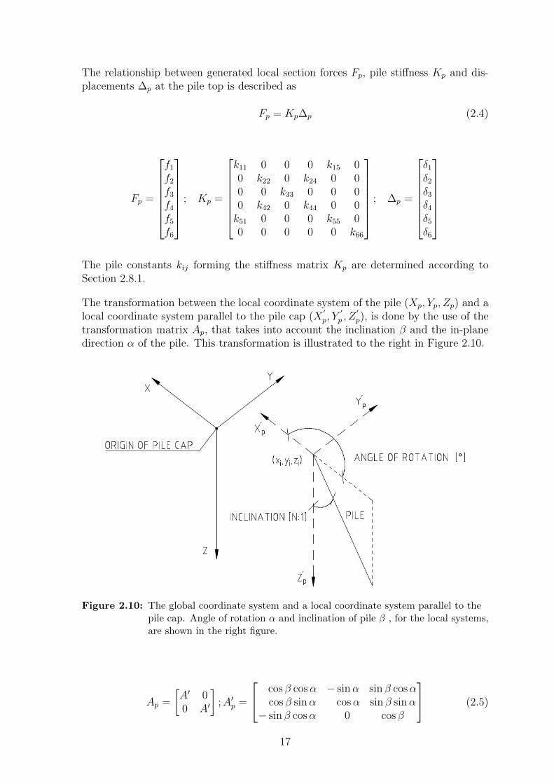
The relationship between generated local section forces Fp, pile stiffness Kp and dis-placements ∆p at the pile top is described as

Fp = Kp∆p (2.4)

Fp =

f1f2f3f4f5f6

; Kp =

k11 0 0 0 k15 00 k22 0 k24 0 00 0 k33 0 0 00 k42 0 k44 0 0k51 0 0 0 k55 00 0 0 0 0 k66

; ∆p =

δ1δ2δ3δ4δ5δ6

The pile constants kij forming the stiffness matrix Kp are determined according toSection 2.8.1.

The transformation between the local coordinate system of the pile (Xp, Yp, Zp) and alocal coordinate system parallel to the pile cap (X

′p, Y

′p , Z

′p), is done by the use of the

transformation matrix Ap, that takes into account the inclination β and the in-planedirection α of the pile. This transformation is illustrated to the right in Figure 2.10.

Figure 2.10: The global coordinate system and a local coordinate system parallel to thepile cap. Angle of rotation α and inclination of pile β , for the local systems,are shown in the right figure.

Ap =

[A′ 00 A′

];A′p =

cos β cosα − sinα sin β cosαcos β sinα cosα sin β sinα

− sin β cosα 0 cos β

(2.5)

17

The total transformation matrix Dp is introduced to take into account the direction,inclination and location of the pile.

Dp = CpAp (2.6)

where Cp takes into account the location and the degree of attachment of the piles.The coordinates of the individual piles in the global system are called x, y and z.These describe the distances between the individual pile and the origin of the pile cap.The degree of attachment between the piles and the pile cap is implemented usingm = 0 for hinged connection and m = 1 for moment stiff connection.

Cp =

1 0 0 0 0 00 1 0 0 0 00 0 1 0 0 00 −z y m 0 0z 0 −x 0 m 0

−y x 0 0 0 m

(2.7)

Since the applied forces are assumed to be known, the displacements of the pile cap canbe calculated using the relationship between the applied forcesR and the displacementsU ;

R = SU (2.8)

U = S−1R (2.9)

where S is the symmetrical stiffness matrix (6x6) where element Sij is the force indirection i which will generate a movement of the pile cap in direction j equal to one.The contributions of all piles are summed in a stiffness matrix at the pile cap origin.

S =n∑

p=1

S ′p (2.10)

whereS ′p = DpKpD

Tp (2.11)

When the global displacements are calculated, the displacements of the piles can bedetermined from

∆p = DTp U (2.12)

Finally, the pile forces and moments Fp are calculated using the relationship betweenthe stiffness of the pile and the displacements (Equation (2.4)). The design pile forcesare determined according to Section 2.8.2.

18

2.8.1 Calculation of Pile Stiffness

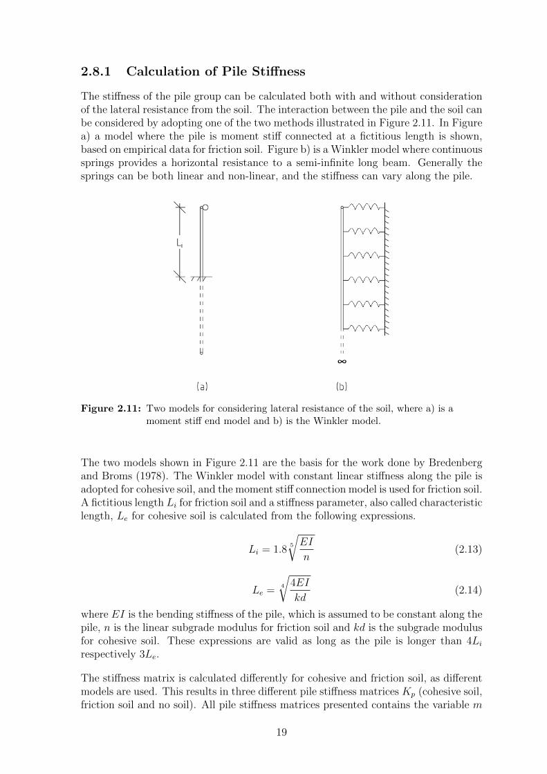
The stiffness of the pile group can be calculated both with and without considerationof the lateral resistance from the soil. The interaction between the pile and the soil canbe considered by adopting one of the two methods illustrated in Figure 2.11. In Figurea) a model where the pile is moment stiff connected at a fictitious length is shown,based on empirical data for friction soil. Figure b) is a Winkler model where continuoussprings provides a horizontal resistance to a semi-infinite long beam. Generally thesprings can be both linear and non-linear, and the stiffness can vary along the pile.

Figure 2.11: Two models for considering lateral resistance of the soil, where a) is amoment stiff end model and b) is the Winkler model.

The two models shown in Figure 2.11 are the basis for the work done by Bredenbergand Broms (1978). The Winkler model with constant linear stiffness along the pile isadopted for cohesive soil, and the moment stiff connection model is used for friction soil.A fictitious length Li for friction soil and a stiffness parameter, also called characteristiclength, Le for cohesive soil is calculated from the following expressions.

Li = 1.85

√EI

n(2.13)

Le =4

√4EI

kd(2.14)

where EI is the bending stiffness of the pile, which is assumed to be constant along thepile, n is the linear subgrade modulus for friction soil and kd is the subgrade modulusfor cohesive soil. These expressions are valid as long as the pile is longer than 4Li

respectively 3Le.

The stiffness matrix is calculated differently for cohesive and friction soil, as differentmodels are used. This results in three different pile stiffness matrices Kp (cohesive soil,friction soil and no soil). All pile stiffness matrices presented contains the variable m

19

that allows for implementing a degree of stiffness of the connection between pile andpile cap where m = 0 for hinged connection and m = 1 for moment stiff connection.

For friction materials, the pile stiffness coefficients derive from the unit displacementsand rotations imposed in Figure 2.12. This is basically from beam theory.

Figure 2.12: The stiffness coefficients for friction soil origin from the resulting forces andmoments from unit displacements and rotations on the moment stiffconnected beam. Axial displacement and twist are not illustrated in thefigure.

The coefficients form the following pile stiffness matrix for friction soil.

Kp =

(3m+ 1)3EI

L3i

0 0 0m6EI

L2i

0

0(3m+ 1)3EI

L3i

0 −m6EI

L2i

0 0

0 0AE

L0 0 0

0 −m6EI

L2i

0m4EI

Li

0 0

m6EI

L2i

0 0 0m4EI

Li

0

0 0 0 0 0mJG

L

(2.15)

For cohesive materials, the pile stiffness coefficients are derived analogously for a beamon elastic foundation. The coefficients form the following pile stiffness matrix forcohesive soil.

20

Kp =

(m+ 1)2EI

L3e

0 0 0m2EI

L2e

0

0(m+ 1)2EI

L3e

0 −m2EI

L2e

0 0

0 0AE

L0 0 0

0 −m2EI

L2e

0m2EI

Le

0 0

m2EI

L2e

0 0 0m2EI

Le

0

0 0 0 0 0mJG

L

(2.16)

If the influence of the soil is ignored, the pile stiffness matrix is formed by the wellknown coefficients for a simply supported beam or a beam with one fixed support andone simple support.

Kp =

m3EI

L30 0 0 0 0

0m3EI

L30 0 0 0

0 0AE

L0 0 0

0 0 0m3EI

L0 0

0 0 0 0m3EI

L0

0 0 0 0 0mJG

L

(2.17)

2.8.2 Calculation of Design Pile Forces

Design section forces are calculated in accordance with Bredenberg and Broms (1978)for each pile so that the resulting stresses can be compared with the permitted values.Maximal shear force fT occur at the pile top and is calculated as the resultant of thehorizontal forces.

fT =√f 21 + f 2

2 (2.18)

The maximal bending moment fM is assumed to occur at the top of the pile for amoment stiff connection and is calculated as

fM =√f 24 + f 2

5 (2.19)

For a hinged connection, the maximal bending moment is assumed by Bredenberg andBroms (1978) to be

21

fM = 0.43fTLi (2.20)

fM = 0.32fTLe (2.21)

The normal force f3 and the twisting moment f6 are considered constant at the sectionsof interest, i.e. where maximum stresses are present.

When verifying the final capacity for the single piles, the location of maximum momentshould be determined as the location where the shear force is zero.

2.8.3 Equilibrium Check

An equilibrium check is carried out to conclude that the calculated result is reliable.This is also described in Bredenberg and Broms (1978), and is done by transformingthe generated forces Fp into a coordinate system that is parallel to the axis of the pilecap.

F ′p = ApFp (2.22)

The transformed forces and moments at the pile top are then in equilibrium with theforce vector Pp in the origin of the pile cap.

Pp = CpF′p (2.23)

The differential between the applied loads at the cap and the sum of all pile forces andmoments will show how accurate the calculations are. The difference should be closeto zero to ensure that there are no errors in the calculations.

R =n∑

p=1

Pp (2.24)

22

3 Method

The development of the pile group optimization program is the primary aim of thisthesis. This requires formulating desired input data and stating an objective function,as well as choosing design variables and state variables and constraints on them. Someof the constraints were based on the results from the interview study presented inSection 2.6. The program was verified by comparing results with an existing programand by testing the optimization function on simple load cases. Four case studies werecarried out to evaluate the program.

An additional study of the often assumed correlation between load center-pile centerdistance and resulting tension forces in the piles was done, using two of the case studiesas reference objects.

3.1 Pile Group Optimization Program

The pile group optimization program was developed in Python. An overview of thestructure of the program is presented in Figure 3.1. The number of piles was a manualinput. Every pile group randomly generated was analyzed for every load case. If thepile group was stable and the generated section forces were smaller than the capacit-ies, it was assessed according to the objective function. The pile group with lowestobjective function was identified as the most optimal pile group. If the optimal pilegroup had low utilization, the number of piles was reduced manually.

Figure 3.1: Flow chart for optimization program.

23

3.1.1 Structural Model and Assumptions

In Section 2.7, important modelling aspects such as rigidity of the pile cap, supportconditions and lateral resistance of the soil were presented. Here, the chosen modeland assumptions for the optimization program is stated.

The pile group calculations were performed both with high and without lateral resist-ance of the soil, regardless of the type of bridge (not only for railway bridges). This isan assumption on the safe side.

The piles were assumed to be end bearing and the pile cap to be infinitely stiff. Forthe no soil calculations, the pile end was hinged, whereas for the soil calculations theconcept of a moment stiff connection at a fictitious length was used for friction soiland the Winkler model was used for cohesive soil, both described in Section 2.7.3.

Displacements and pile forces were calculated according to the frame analysis methoddescribed in Section 2.8.

The cross section was chosen to be the same for all piles in the pile group. This wasdone due to practical reasons concerning equipment and pile machines described inSection 2.6. Also, the pile length was the same for all piles, which is a limitation.

3.1.2 Input Data

The following input data, that the designer could define, was implemented in theprogram.

• Loads: The loads (3 forces, 3 moments), for each load case, applied to the pilecap origin at the cut-off level of the piles.

• Number of piles: Chosen from experience or estimated based on simple calcula-tions.

• Pile capacity: The pile capacity was implemented according to ultimate limitstate using a simplified method shown in Section 3.1.5.

• Deformation: Allowable deformation for the pile cap.

• Pile top conditions: Options fixed or hinged.

• Pile parameters: Geometrical data such as pile length and dimensions of crosssection, and material properties (Young’s modulus and shear modulus).

• Soil parameters: Options for soil type were cohesive or friction soil, and corres-ponding soil parameters subgrade modulus or linear subgrade modulus.

• Pile cap: The dimensions of the pile cap in both x- and y-direction.

• Symmetry: The pile group could be restricted to either double or single sym-metry.

24

3.1.3 Objective Function

Based on the general expression of structural optimization (SO) presented by Christensenet al. (2008), an objective function was formulated.

SO =

minimize f(a, b(a)) with respect to a and b

subject to

design constraints on a

behavioral constraints on b

equilibrium constraints

where

f(a, b(a)) is the objective function

a is a function or vector that describes the design

b is a function or vector that represents the response of the structure for a given a,

also called state variables

The objective function f was stated to describe the force difference between the max-imum normal force and the minimum normal force in the piles. It measured thedistribution of forces in the pile group and was formulated as

f = max(NEd,max) −min(NEd,min) (3.1)

High value of f meant large difference between the maximum and minimum normalforces, and vice versa. The structural optimization intended to decrease the differencebetween the maximum and minimum normal forces in the pile group. The objectivefunction was evaluated in parallel for conditions with and without lateral resistancefrom the soil, where the highest objective function was decisive for the pile group.

The variables were the design variables a and the state variables b, which are describedin detail in the following section.

3.1.4 Variables

The design variables a had uniform distribution and varied during optimization. Theyformed a matrix with n rows, where n was the number of piles.

a =

ai...an

; i = [1, 2, ..., n]

Every pile i had four parameters that could vary. With a coordinate system definedas in Section 2.8 the parameters were formulated in a vector ai as (see Figure 2.10)

ai =[xi yi αi βi

]25

where

xi is the x-coordinate

yi is the y-coordinate

αi is the in plane direction of the pile

βi is the inclination of the pile

The state variables b were chosen to represent the response of the structure, andincluded section forces bi for every pile i and deformations U for the total system.

b = f(a) =

{bi

U

where f(a) represent Equation (2.4)-(2.11). The generalized section forces consistedof 3 forces and 3 moments at every pile top.

bi =[Ni,xEd Ni,yEd Ni,zEd Mi,xEd Mi,yEd Mi,zEd

]The deformations were presented as 3 translations and 3 rotations at the pile cap.

U =[ux uy uz wx wy wz

]3.1.5 Constraints

The constraints were divided into design constraints, behavioral constraints and equi-librium constraints. The upper and lower bounds were, for some parameters, chosenby the designer and, for others, determined in the program.

As described in Section 3.1.4, the pile had parameters that could vary. Due to geo-metrical limitations the coordinates (x, y) of the pile could only vary within the limitsof the pile cap. The minimum allowable pile distances were also constraining the pilecoordinates. A minimum distance of 0.8 meter was used as constraint in the program.However, the pile distance 0.8 meter is only valid for piles leaning away from eachother, as described in Section 2.5.1. The check of whether this assumption is true,is left for the user to ensure. Since there are limitations of the pile equipment andsafety requirements for the working environment, the inclination β of the piles waslimited to 4:1. The in plane direction α of the piles was also limited by only lettingthe piles lean away from the origin of the pile cap. The number of possible directions αand inclinations β were limited by the user. The more options, the more optimal pilegroups can be found, but the simulations take longer time to complete. This flexibilityallows for a reasonable number of options for the specific case studied.

The behavioral constraints used in the program were the limitation of allowable sec-tion forces due to ultimate limit state and allowable deformations. These parametersdepend on selected pile type, cross section and the geotechnical conditions, and shouldbe defined by the user. Interaction of normal force and moment for steel and timber

26

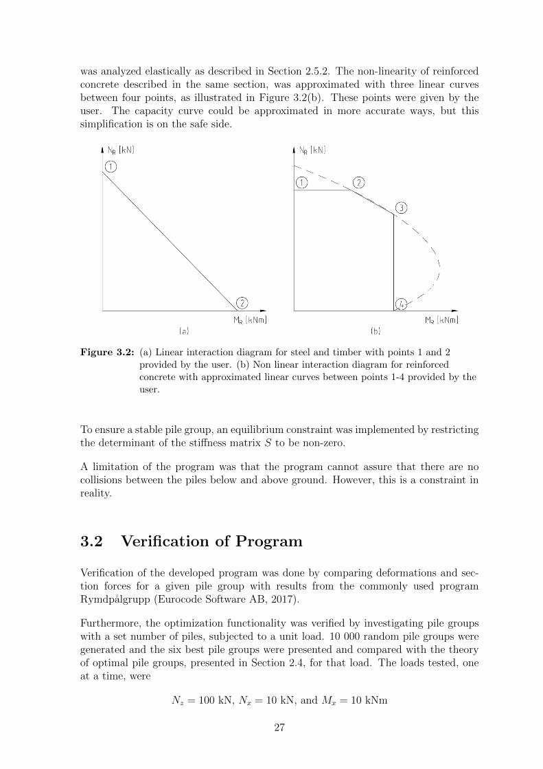
was analyzed elastically as described in Section 2.5.2. The non-linearity of reinforcedconcrete described in the same section, was approximated with three linear curvesbetween four points, as illustrated in Figure 3.2(b). These points were given by theuser. The capacity curve could be approximated in more accurate ways, but thissimplification is on the safe side.

Figure 3.2: (a) Linear interaction diagram for steel and timber with points 1 and 2provided by the user. (b) Non linear interaction diagram for reinforcedconcrete with approximated linear curves between points 1-4 provided by theuser.

To ensure a stable pile group, an equilibrium constraint was implemented by restrictingthe determinant of the stiffness matrix S to be non-zero.

A limitation of the program was that the program cannot assure that there are nocollisions between the piles below and above ground. However, this is a constraint inreality.

3.2 Verification of Program

Verification of the developed program was done by comparing deformations and sec-tion forces for a given pile group with results from the commonly used programRymdpalgrupp (Eurocode Software AB, 2017).

Furthermore, the optimization functionality was verified by investigating pile groupswith a set number of piles, subjected to a unit load. 10 000 random pile groups weregenerated and the six best pile groups were presented and compared with the theoryof optimal pile groups, presented in Section 2.4, for that load. The loads tested, oneat a time, were

Nz = 100 kN, Nx = 10 kN, and Mx = 10 kNm

27

These loads are much lower than real loads acting on a pile foundation for a bridge.They are only used to evaluate the conceptual arrangement of the pile group.

3.3 Case Studies

Four case studies were carried out of pile groups already designed, and some of themalready built. The cases chosen were mid support and abutment of a pedestrian bridge,mid support of a road bridge and abutment of a railway bridge. The existing designswere shared by the owners of the bridges and were compared to the designs resultingfrom the random pile group generator.

Input data for all case studies is presented in a summarized table in Section 3.3.4. Allinput data, including the applied loads, is presented in Appendix C-F. The externalforces are in all cases applied at the origin of the pile cap, at the pile cut-off level. Allpile groups were designed for load combinations in ultimate limit state. When simu-lating random pile groups, background information from the existing pile group wasused with some exceptions. The most important differences between the assumptionsmade for the reference pile groups and the assumptions made in this project, is thelateral resistance of the soil and the inclination of piles. In this project, calculationswere made for both lateral resistance of the soil and no lateral resistance of the soil andthe maximal inclination was set to 4:1. As mentioned before, the angle of rotation ofthe piles varied with different increments, depending on the complexity of the specificcase.

3.3.1 Case I and II - Pedestrian Bridge Mid Support andAbutment

The pedestrian bridge was built in 2019, across Harlovsangaleden in Kristianstad. Thesubstructure of the bridge consists of two abutments and two mid supports, see Figure3.3.

28

Figure 3.3: Elevation of half of the pedestrian bridge showing abutment (1) and midsupport (2). Figure adapted from Kristianstad Municipality (2019).

For Case I, the mid support was investigated. The existing pile group was symmetricaround two axes and had 8 reinforced concrete piles, all with the inclination 3.5:1.

For the random pile group generator, 8 piles in a double-symmetric arrangement wasused. The inclination options were 4:1, 8:1 and vertical, and the rotation varied in15o-increments.

The abutment of the same pedestrian bridge as in Case I was used for Case II, seeFigure 3.3. The existing pile group was symmetric around the x-axis and had 6reinforced concrete piles. As for Case I, the piles had the inclination 3.5:1.

For Case II, the random pile group generator produced pile groups with 6 piles sym-metric around the x-axis. The inclination options were 4:1, 8:1 and vertical, and therotation varied in 15o-increments.

3.3.2 Case III - Road Bridge Mid Support

The third case was a road bridge along the E45 road, over the eastern entrance of theMarieholm tunnel in Gothenburg. The structure was built in 2015. An overview of apart of the bridge is given in Figure 3.4.

29

Figure 3.4: Overview of the bridge. Elevation for Case III. The intermediate support (7)is the one investigated in this case study. Figure adapted from Trafikverket(2015).

The existing pile group was symmetric around two axes and had 28 piles with theinclinations 20:1, 12:1 and 8:1.

The random pile group generator was tested with 24 piles, symmetric around two axes.The pile inclination possibilities were 4:1, 8:1 and vertical, and the angle of rotationwas free to vary in 45o-increments.

30

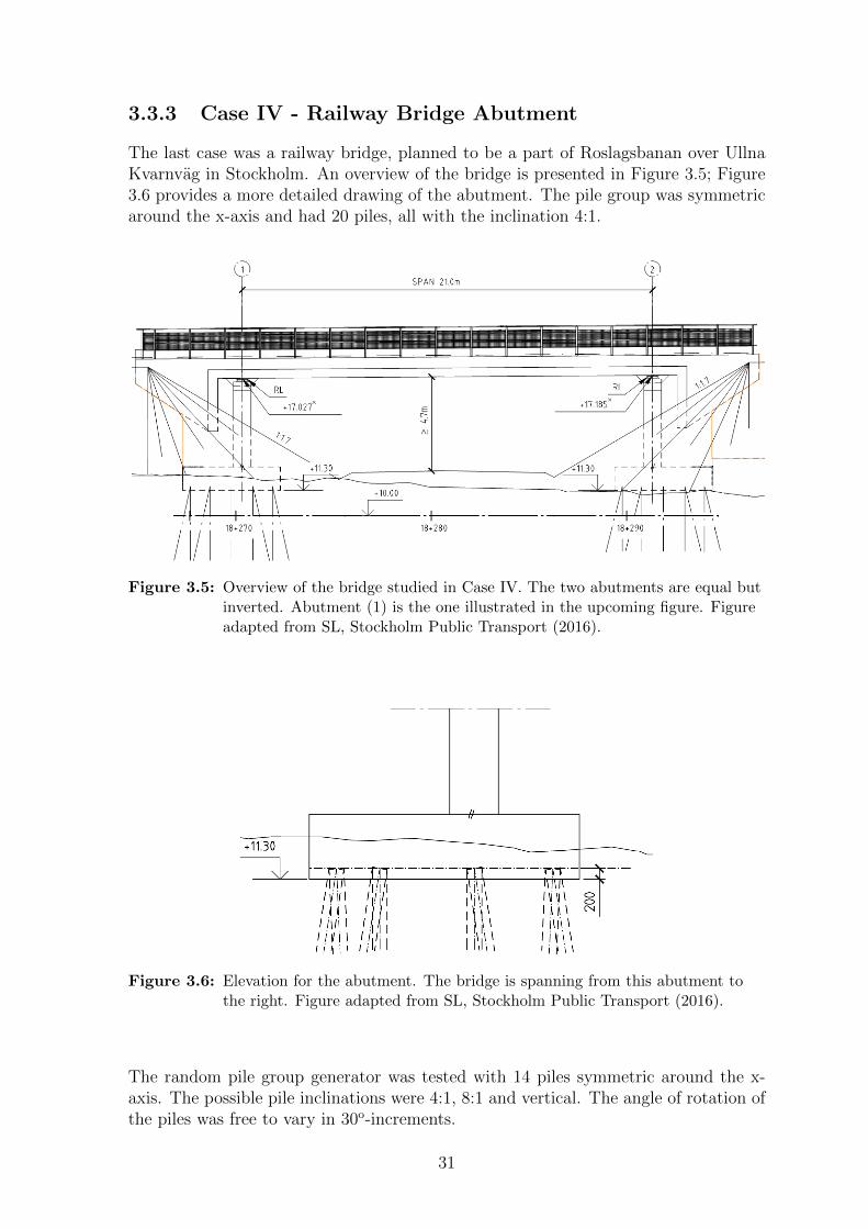
3.3.3 Case IV - Railway Bridge Abutment

The last case was a railway bridge, planned to be a part of Roslagsbanan over UllnaKvarnvag in Stockholm. An overview of the bridge is presented in Figure 3.5; Figure3.6 provides a more detailed drawing of the abutment. The pile group was symmetricaround the x-axis and had 20 piles, all with the inclination 4:1.

Figure 3.5: Overview of the bridge studied in Case IV. The two abutments are equal butinverted. Abutment (1) is the one illustrated in the upcoming figure. Figureadapted from SL, Stockholm Public Transport (2016).

Figure 3.6: Elevation for the abutment. The bridge is spanning from this abutment tothe right. Figure adapted from SL, Stockholm Public Transport (2016).

The random pile group generator was tested with 14 piles symmetric around the x-axis. The possible pile inclinations were 4:1, 8:1 and vertical. The angle of rotation ofthe piles was free to vary in 30o-increments.

31

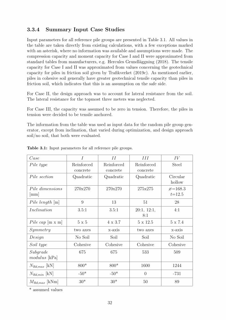
3.3.4 Summary Input Case Studies

Input parameters for all reference pile groups are presented in Table 3.1. All values inthe table are taken directly from existing calculations, with a few exceptions markedwith an asterisk, where no information was available and assumptions were made. Thecompression capacity and moment capacity for Case I and II were approximated fromstandard tables from manufacturers, e.g. Hercules Grundlaggning (2018). The tensilecapacity for Case I and II was approximated from values concerning the geotechnicalcapacity for piles in friction soil given by Trafikverket (2019c). As mentioned earlier,piles in cohesive soil generally have greater geotechnical tensile capacity than piles infriction soil, which indicates that this is an assumption on the safe side.

For Case II, the design approach was to account for lateral resistance from the soil.The lateral resistance for the topmost three meters was neglected.

For Case III, the capacity was assumed to be zero in tension. Therefore, the piles intension were decided to be tensile anchored.

The information from the table was used as input data for the random pile group gen-erator, except from inclination, that varied during optimization, and design approachsoil/no soil, that both were evaluated.

Table 3.1: Input parameters for all reference pile groups.

Case I II III IV

P ile type Reinforcedconcrete

Reinforcedconcrete

Reinforcedconcrete

Steel

Pile section Quadratic Quadratic Quadratic Circularhollow

Pile dimensions[mm]

270x270 270x270 275x275 �=168.3t=12.5

Pile length [m] 9 13 51 28

Inclination 3.5:1 3.5:1 20:1, 12:1,8:1

4:1

Pile cap [m x m] 5 x 5 4 x 3.7 5 x 12.5 5 x 7.4

Symmetry two axes x-axis two axes x-axis

Design No Soil Soil Soil No Soil

Soil type Cohesive Cohesive Cohesive Cohesive

Subgrademodulus [kPa]

675 675 533 509

NRd,max [kN] 800* 800* 1600 1244

NRd,min [kN] -50* -50* 0 -731

MRd,max [kNm] 30* 30* 50 89

* assumed values

32

3.4 Investigation of Distance Between Pile Center

and Load Center

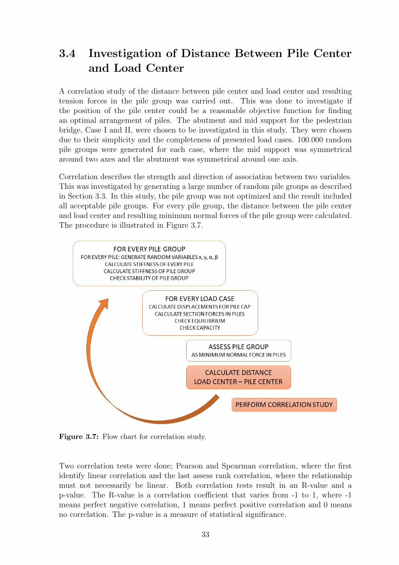
A correlation study of the distance between pile center and load center and resultingtension forces in the pile group was carried out. This was done to investigate ifthe position of the pile center could be a reasonable objective function for findingan optimal arrangement of piles. The abutment and mid support for the pedestrianbridge, Case I and II, were chosen to be investigated in this study. They were chosendue to their simplicity and the completeness of presented load cases. 100.000 randompile groups were generated for each case, where the mid support was symmetricalaround two axes and the abutment was symmetrical around one axis.

Correlation describes the strength and direction of association between two variables.This was investigated by generating a large number of random pile groups as describedin Section 3.3. In this study, the pile group was not optimized and the result includedall acceptable pile groups. For every pile group, the distance between the pile centerand load center and resulting minimum normal forces of the pile group were calculated.The procedure is illustrated in Figure 3.7.

Figure 3.7: Flow chart for correlation study.

Two correlation tests were done; Pearson and Spearman correlation, where the firstidentify linear correlation and the last assess rank correlation, where the relationshipmust not necessarily be linear. Both correlation tests result in an R-value and ap-value. The R-value is a correlation coefficient that varies from -1 to 1, where -1means perfect negative correlation, 1 means perfect positive correlation and 0 meansno correlation. The p-value is a measure of statistical significance.

33

Pile center is a location that depends on the stiffness of the piles and the soil whereasload center is a location that depends on the loads applied. The pile center has a strictmathematical definition that is presented below, but as load center can be interpretedin several ways and little is written in the literature about it, three different methodswere tested. All calculations were done in the global coordinate system presented inSection 2.8.

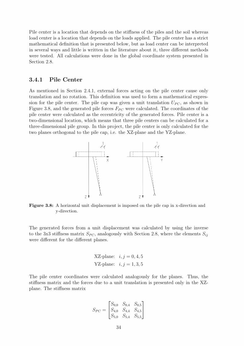
3.4.1 Pile Center

As mentioned in Section 2.4.1, external forces acting on the pile center cause onlytranslation and no rotation. This definition was used to form a mathematical expres-sion for the pile center. The pile cap was given a unit translation UPC , as shown inFigure 3.8, and the generated pile forces FPC were calculated. The coordinates of thepile center were calculated as the eccentricity of the generated forces. Pile center is atwo-dimensional location, which means that three pile centers can be calculated for athree-dimensional pile group. In this project, the pile center is only calculated for thetwo planes orthogonal to the pile cap, i.e. the XZ-plane and the YZ-plane.

Figure 3.8: A horizontal unit displacement is imposed on the pile cap in x-direction andy-direction.

The generated forces from a unit displacement was calculated by using the inverseto the 3x3 stiffness matrix SPC , analogously with Section 2.8, where the elements Sij

were different for the different planes.

XZ-plane: i, j = 0, 4, 5

YZ-plane: i, j = 1, 3, 5

The pile center coordinates were calculated analogously for the planes. Thus, thestiffness matrix and the forces due to a unit translation is presented only in the XZ-plane. The stiffness matrix

SPC =

S0,0 S0,4 S0,5

S4,0 S4,4 S4,5

S5,0 S5,4 S5,5

34

The unit displacement

UPC =

U0

U4

U5

=

100

The generated forces were calculated as

FPC =

f0f4f5

= S−1PCU (3.2)

The pile center coordinates (PCx, PCzx) in the XZ-plane could be calculated as theeccentricity of the generated forces. PCzx is the z-coordinate in the XZ-plane.

PCx =−f5f0

(3.3)

PCzx =f4f0

(3.4)

This is the coordinates that should be compared to the load center.

3.4.2 Load Center

Three approaches were tested for calculating the load center - the broom method, themean value method and the center of mass method.

All three methods starts by transforming moments into loads with an eccentricity inthe pile cut-off plane. The concept of this transformation is illustrated in Figure 3.9.

Figure 3.9: Eccentricity concept. The moment is replaced with an eccentricity.

For the broom method, inclined loads were placed at the pile cut-off level, forming abroom. This is a graphical method described in old handbooks, e.g. Stal (1984), thatdepicts the load center as the smallest part of the broom created by all load cases.The loads were elongated, see Figure 3.10, and the smallest part of the broom was

35

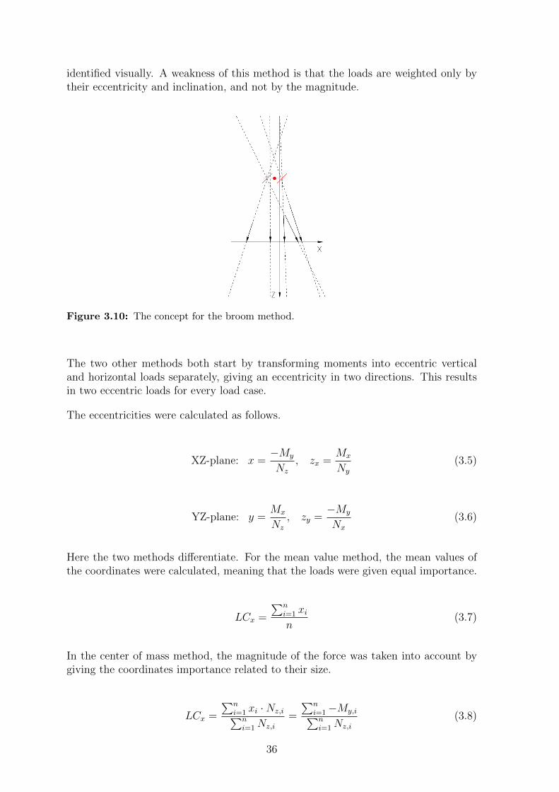
identified visually. A weakness of this method is that the loads are weighted only bytheir eccentricity and inclination, and not by the magnitude.

Figure 3.10: The concept for the broom method.

The two other methods both start by transforming moments into eccentric verticaland horizontal loads separately, giving an eccentricity in two directions. This resultsin two eccentric loads for every load case.

The eccentricities were calculated as follows.

XZ-plane: x =−My

Nz

, zx =Mx

Ny

(3.5)

YZ-plane: y =Mx

Nz

, zy =−My

Nx

(3.6)

Here the two methods differentiate. For the mean value method, the mean values ofthe coordinates were calculated, meaning that the loads were given equal importance.

LCx =

∑ni=1 xin

(3.7)

In the center of mass method, the magnitude of the force was taken into account bygiving the coordinates importance related to their size.

LCx =

∑ni=1 xi ·Nz,i∑n

i=1Nz,i

=

∑ni=1−My,i∑ni=1Nz,i

(3.8)

36

3.4.3 Distance Between Pile Center and Load Center

The distance between the center of piles and the center of loads was calculated ana-logously in two planes, XZ and YZ.

dXZ =

√(PCx − LCx)2 + (PCzx − LCzx)2 (3.9)

dY Z =

√(PCy − LCy)

2 + (PCzy − LCzy)2 (3.10)

For every pile group, the total distance was calculated as the sum of these distancesas

Distance = dXZ + dY Z (3.11)

where the total distance was used, together with the resulting tension forces, in thecorrelation study.

37

4 Results

In this section the results will be presented. In short, the developed program wassuccessful in producing suitable pile groups for unit loads. It could present adequatepile groups for all four case studies. The correlation study indicates that the distancebetween the pile center and the load center may not be a good basis for optimization.

4.1 Verification of Program

Pile groups subjected to a specific unit load was generated by the program. The loadswere

Nz = 100 kN, Nx = 10 kN, and Mx = 10 kNm

For every unit load, the six best pile groups were presented. All results can be found inAppendix B. Here, only one representative pile group for every unit load is presented.

In Figure 4.1, the pile group is subjected to a horizontal force in one direction only,which results in many inclined piles in the direction of the load. The pile plot is aview of the pile cap and the piles from above, where the pile top and pile end (andtherefore also the inclination and direction) are shown.

Figure 4.1: Nx = 10 kN. Most piles lean in the x-direction.

Figure 4.2 shows a pile group generated from a vertical load. This pile group has afew slightly inclined piles for stability, but most piles are vertical.

39

Figure 4.2: Nz = 100 kN. Most piles are vertical.

A pile group subjected to a moment around one axis was arranged by the programas seen in Figure 4.3. A moment around the x-axis is handled by a long lever armbetween piles in the y-direction.

Figure 4.3: Mx = 10 kNm. Piles are arranged parallel with a large distance in they-direction.

The, by the program, generated pile groups for the unit loads are in line with expect-ations from basic concepts for pile group arrangement.

40

4.2 Case Studies

The developed program could present adequate pile groups for all four case studies.Section forces for the reference pile groups, both from existing calculations and recal-culated using the developed software, and section forces for the simulated pile groups,are presented in tables in the following sections. The values are matching for all casesexcept Case II. The existing pile groups are denoted with Ref in the tables and arefollowed by the three best simulated pile groups in descending order. The most op-timal simulated pile group, due to the objective function, is also presented in figuresin the upcoming sections, while the rest are presented in figures in Appendix C-F. Theexternal loads, applied at origin, are found in the same appendices.

4.2.1 Case I - Pedestrian Bridge Mid Support

The eight piles were arranged symmetrical around two axes, which means that thereare only two piles that are randomly generated, and the number of possible arrange-ments is therefore limited. When running the simulation repetitively, few pile groupsare acceptable and the same acceptable pile groups reoccur. This means that therestrictions are strict, and according to further investigations of the constraints, theminimum normal force is the variable constraining the simulation.

100 000 pile groups were generated in a simulation that took 1 hour and 5 minutes, ofwhich 78 were acceptable pile groups, where duplicates were detected. The simulationresulted in pile groups similar to the existing one. Figure 4.4 shows the reference pilegroup, Figure 4.5 shows the best simulated pile group, and Figure 4.6-4.7 shows theresulting section forces for both pile groups along with the capacity curve.

Figure 4.4: Pedestrian bridge mid support. The reference pile group with 8 piles.

41

Figure 4.5: Pedestrian bridge mid support. The best simulated pile group with 8 piles.

Figure 4.6: Pedestrian bridge mid support. Section forces for the reference pile group.One dot represent one load case and one pile. The blue line is the capacitycurve.

42

Figure 4.7: Pedestrian bridge mid support. Section forces for the best simulated pilegroup.

Table 4.1 shows calculated section forces for the reference pile group and the threebest simulated pile groups, all with and without lateral resistance of the soil. Themaximum normal forces were similar to the reference pile group, whereas the tensionforces were larger.

Table 4.1: Calculated section forces.

PileGroup

Soil/No Soil

Nmax

[kN]Nmin

[kN]Vmax

[kN]Mmax

[kNm]Nmax −Nmin

[kN]

Values from existing calculations

Ref No Soil 481 -3 0 0 N/A

Values from developed software

Ref Soil 465 3 1 2 462

Ref No Soil 481 -3 0 0 484

1 Soil 470 -2 2 2 472

1 No Soil 473 -19 0 0 491

2 Soil 461 -15 2 2 475

2 No Soil 472 -27 0 0 499

3 Soil 459 -13 2 2 471

3 No Soil 479 -30 0 0 508

The reference pile group was designed with pile inclination 3.5:1, while the maximumallowed inclination for the developed software was 4:1, due to safety reasons. Since theratio between the applied horizontal loads and vertical loads are relatively large forthe pedestrian bridge, increased inclination of the piles will reduce tension. In otherwords, if larger inclination would be allowed in the developed program, tension forces

43

would probably be lower than for the reference pile group.

4.2.2 Case II - Pedestrian Bridge Abutment

100.000 pile groups were generated in the simulation, where 139 pile groups met therequirements. The duration time was 26 minutes. The pile plot for the best simulatedpile group is presented, together with the reference pile group, in Figure 4.8. Thesimulated pile group is unfeasible as there are piles colliding.

Figure 4.8: Pedestrian bridge abutment. To the left: The reference pile group with 6piles. To the right: The best simulated pile group with 6 piles.

44

The section forces for the best pile group, together with the reference pile group, isshown in Figure 4.9.

Figure 4.9: Pedestrian bridge abutment. Upper figure: Section forces for the referencepile group. Lower figure: Section forces for the best simulated pile group.

45

The section forces for the three best pile groups are presented in Table 4.2.

Table 4.2: Calculated section forces.

PileGroup

Soil/No Soil

Nmax

[kN]Nmin

[kN]Vmax

[kN]Mmax

[kNm]Nmax −Nmin

[kN]


Ref Soil 614 5 2 N/A N/A


Ref Soil 588 37 7 8 551

Ref No Soil 621 -3 0 0 624

1 Soil 541 90 6 7 451

1 No Soil 552 61 0 0 491

2 Soil 546 91 7 7 455

2 No Soil 555 47 0 0 508

3 Soil 579 53 5 5 526

3 No Soil 620 52 0 0 568

The simulated pile groups had somewhat smaller maximum normal forces than thereference pile group, and considerably higher minimum normal forces. The risk forhaving tension in the generated pile groups due to imprecise installation is lower forthe simulated pile groups than for the reference pile group, i.e. it is more robust.The minimum normal forces were increased, despite having less inclined piles. Thisindicates that a smart arrangement of the piles allows for smaller inclination of thepiles, which is positive for installation purposes.

As mentioned earlier, the reference values calculated in the program were somewhatdifferent compared to the existing calculations. This is probably due to an assumptionof having no lateral soil resistance in the topmost three meters that was made in theoriginal calculations.

4.2.3 Case III - Road Bridge Mid Support

The road bridge of Marieholm was originally calculated with lateral resistance fromcohesive soil. However, the section forces for the reference pile group are also calculatedwithout any soil, to be able to compare with the simulation. Generated section forcesfor the best pile groups with 24 piles are presented in Table 4.3. 100 000 pile groupswere generated in a simulation that took 1 hour and 5 minutes, of which 34 pile groupsmet the requirements.

The existing pile group and the best simulated pile group are shown in Figure 4.10.As can be seen in the figure, the simulated pile group is less organized and there arerisks of collisions between some of the piles. The section forces for the existing pilegroup and the best simulated pile group are illustrated in Figure 4.11.

46

Figure 4.10: Road bridge mid support: Upper figure: The reference pile group with 28piles. Lower figure: The best simulated pile group with 24 piles.

47

Figure 4.11 shows that the reference pile group would not have met the requirementsfor compression and tension if calculations had been performed without respect to thelateral resistance of the soil. According to Trafikverket (2019a), this is not requiredfor a road bridge, as long as both high and low values for the lateral resistance isconsidered.

Figure 4.11: Road bridge mid support. Upper figure: Section forces for the reference pilegroup. Lower figure: Section forces for the best simulated pile group.

48

Table 4.3: Calculated section forces with 24 piles.

PileGroup

Soil/No Soil

Nmax

[kN]Nmin

[kN]Vmax

[kN]Mmax

[kNm]Nmax −Nmin

[kN]


Ref Soil 1183 -103 26 28 N/A


Ref Soil 1183 -103 26 28 1286

Ref No Soil 2056 -1142 0 0 3198

1 Soil 1338 -45 15 16 1382

1 No Soil 1359 -138 0 0 1488

2 Soil 1363 -88 14 15 1450

2 No Soil 1377 -174 0 0 1550

3 Soil 1424 -122 15 16 1546

3 No Soil 1446 -129 0 0 1574

All normal forces calculated without any lateral resistance from the soil are better forthe presented simulated pile groups than for the reference pile group. As mentionedbefore, the reference pile group was originally only calculated with lateral resistancefrom the soil. For the calculations with soil, the pile group simulation did not manageto generate pile groups with lower compression forces than the reference pile group.However, the simulation performed well for tension forces. The simulation even man-aged to find solutions with fewer piles as input than the reference pile group.

4.2.4 Case IV - Railway Bridge Abutment

The railway bridge over Ullna Kvarnvag was originally calculated without lateral res-istance from the soil. However, the section forces for the reference pile group are alsocalculated with soil, to be able to compare with the simulation. 10 000 random pilegroups were generated in the investigation, of which 843 pile groups met the require-ments. The duration of the simulation was less than 5 minutes.

The reference pile group and the best simulated pile group are shown in Figure 4.12.As can be seen in the figure for the best simulated pile group, it is not obvious if somepiles will collide or not. The corresponding section forces are presented in Figure 4.13.

49

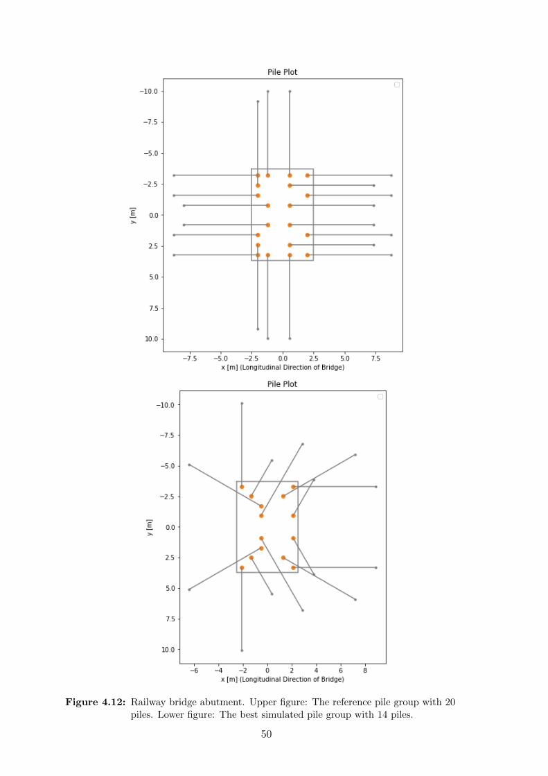
Figure 4.12: Railway bridge abutment. Upper figure: The reference pile group with 20piles. Lower figure: The best simulated pile group with 14 piles.

50

Figure 4.13: Railway bridge abutment. Upper figure: Section forces for the reference pilegroup. Lower figure: Section forces for the best simulated pile group.

51

Generated section forces for the reference pile group and for the three best simulatedpile groups with 14 piles are presented in Table 4.4.

Table 4.4: Calculated section forces with 14 piles.

PileGroup

Soil/No Soil

Nmax

[kN]Nmin

[kN]Vmax

[kN]Mmax

[kNm]Nmax −Nmin

[kN]


Ref No Soil 744 -51 0 0 N/A


Ref Soil 754 69 11 8 685

Ref No Soil 744 -51 0 0 795

1 Soil 828 339 13 9 490

1 No Soil 852 305 0 0 546

2 Soil 834 309 10 8 525

2 No Soil 853 229 0 0 623

3 Soil 926 336 10 8 590

3 No Soil 935 261 0 0 674

The pile group simulation produced pile groups with lower objective function than forthe reference pile group, meaning that the distribution of forces between the piles weremore even. These results were generated by only 14 piles, i.e. a reduction of six piles.

52

4.2.5 Summary Case Studies

To make it easier to analyze the results, an overview of the results for all cases ispresented in Table 4.5. The values in the table are differences between the mostoptimal simulated pile groups and the reference pile groups. The difference has beencalculated for maximum normal force, minimum normal force, the objective functionand the number of reduced piles. If the simulated pile group is an improvementcompared with the reference pile group, the difference is negative, and vice versa. Theimproved values are also highlighted with green color.

Table 4.5: The difference between the most optimal simulated pile groups and thereference pile groups, presented for maximum and minimum normal force andobjective function. The number of reduced piles is also presented for everycase study.

The existing designs were originally calculated only with or without lateral resistancefrom the soil, unlike the developed software that took both into account. As describedin Section 3.1.3, the objective function was evaluated in parallel for conditions withand without lateral resistance from the soil, where the highest objective function wasdecisive for the pile group. If the program had performed calculations using only thesame assumption of soil used in the existing design, the generated results would havebeen positively affected.

For Case I, the developed program did not manage to produce pile groups with bettersection forces than the reference pile group. However, the differences were small.

The arrangement of piles for the simulated pile group in Case II, did both decreasethe maximum normal force and increase the minimum normal force.

The simulated pile group in Case III, had a reduction of four piles compared to thereference pile group. Once again, the reference pile group did only consider lateralresistance from the soil. Therefore, the high negative values do not undermine theexisting design, but were only used to evaluate the influence of the soil.

53

For Case IV, the simulated pile group had a reduction of six piles compared withthe reference pile group. The minimum normal forces were significantly improved.However, the maximum normal forces were lower for the reference pile group.

54

4.3 Investigation of Distance Between Pile Center

and Load Center

Two case studies were carried out for the correlation tests. For both cases, the calcu-lated load center is presented first. This value does not change during the simulation,in contradiction to the pile center, that is unique for every simulated pile group. Then,correlation plots and values are presented.

4.3.1 Case I - Pedestrian Bridge Mid Support

Coordinates for the load center calculated in three different ways are presented inTable 4.6. The coordinates for the broom method was evaluated visually from Figure4.14.

Figure 4.14: Case I: The broom created by all elongated load cases placed at the pilecut-off plane. Load center for the broom method was evaluated visuallyfrom these figures.

According to Table 4.6, the calculated coordinates for the load center became similarfor all three methods, except for the coordinate LCzy, which differed significantlybetween the broom method and the other two methods.

Table 4.6: Case I: Coordinates for the load center in XZ- and YZ-plane.

Method LCx [m] LCzx [m] LCy [m] LCzy [m]

The broom -0.1 -7.1 0 -7.7

The mean value -0.12 -7.69 -0.02 -23.83

The center of mass -0.13 -6.27 -0.02 -25.25

10.000 random pile groups were generated in this investigation. 601 of them wereacceptable pile groups that were used for the correlation test. The resulting minimum

55

normal force in the pile group and the distance load center - pile center is plotted inFigure 4.15. The result from the correlation tests is presented in Table 4.7, 4.8 and4.9.

Figure 4.15: Case I: Correlation between resulting minimum normal forces and thedistance between pile center and load center, for the three different methodsfor calculating the load center.

56

Table 4.7: Case I: Correlation coefficient and two-tailed p-value with the broom method.

CorrelationType

Soil/No Soil CorrelationCoefficient R

p-value Classification

Pearson Soil 0.078 0.056 not significant

Pearson No Soil -0.040 0.033 negligible correlation

Spearman Soil 0.100 0.014 negligible correlation

Spearman No Soil -0.012 0.767 not significant

Table 4.8: Case I: Correlation coefficient and two-tailed p-value with the mean valuemethod.

CorrelationType



Pearson Soil 0.288 6 · 10−13 low positive correlation

Pearson No Soil 0.214 1 · 10−7 low positive correlation

Spearman Soil 0.287 8 · 10−13 low positive correlation

Spearman No Soil 0.213 1 · 10−7 low positive correlation

Table 4.9: Case I: Correlation coefficient and two-tailed p-value with the center of massmethod.

CorrelationType



Pearson Soil 0.193 2 · 10−6 negligible correlation

Pearson No Soil 0.144 0.0004 negligible correlation

Spearman Soil 0.186 4 · 10−6 negligible correlation

Spearman No Soil 0.140 0.0006 negligible correlation

The results differed between the three methods. The broom method did not show asignificant correlation. For the mean value method and the center of mass method,negligible or low positive correlation was found in the investigation of the relationshipbetween pile center and load center, and the resulting minimum normal forces in thepile group.

57

4.3.2 Case II - Pedestrian Bridge Abutment

Coordinates for the load center calculated in three different ways are presented inTable 4.10. The coordinates for the broom method was evaluated visually from Figure4.16.

Figure 4.16: Case II. The broom created by all elongated load cases placed at the pilecut-off plane. Load center for the broom method was evaluated visuallyfrom these figures.

Table 4.10 shows that the coordinates for the load center differed depending on whichmethod was used, especially for the LCzy-coordinate.

Table 4.10: Case II: Coordinates for the load center in XZ- and YZ-plane.

Method LCx [m] LCzx [m] LCy [m] LCzy [m]

The broom -1.35 -4 0 -1.5

The mean value -1.05 3.50 0.00 22.51

The center of mass -1.05 0.45 0.00 17.17

40.000 random pile groups were generated in this investigation. 587 of them wereacceptable pile groups that were used for the correlation test. The objective functionand distance load center - pile center is plotted in Figure 4.17.

58

Figure 4.17: Case II: Correlation between resulting minimum normal forces and thedistance between pile center and load center.

59

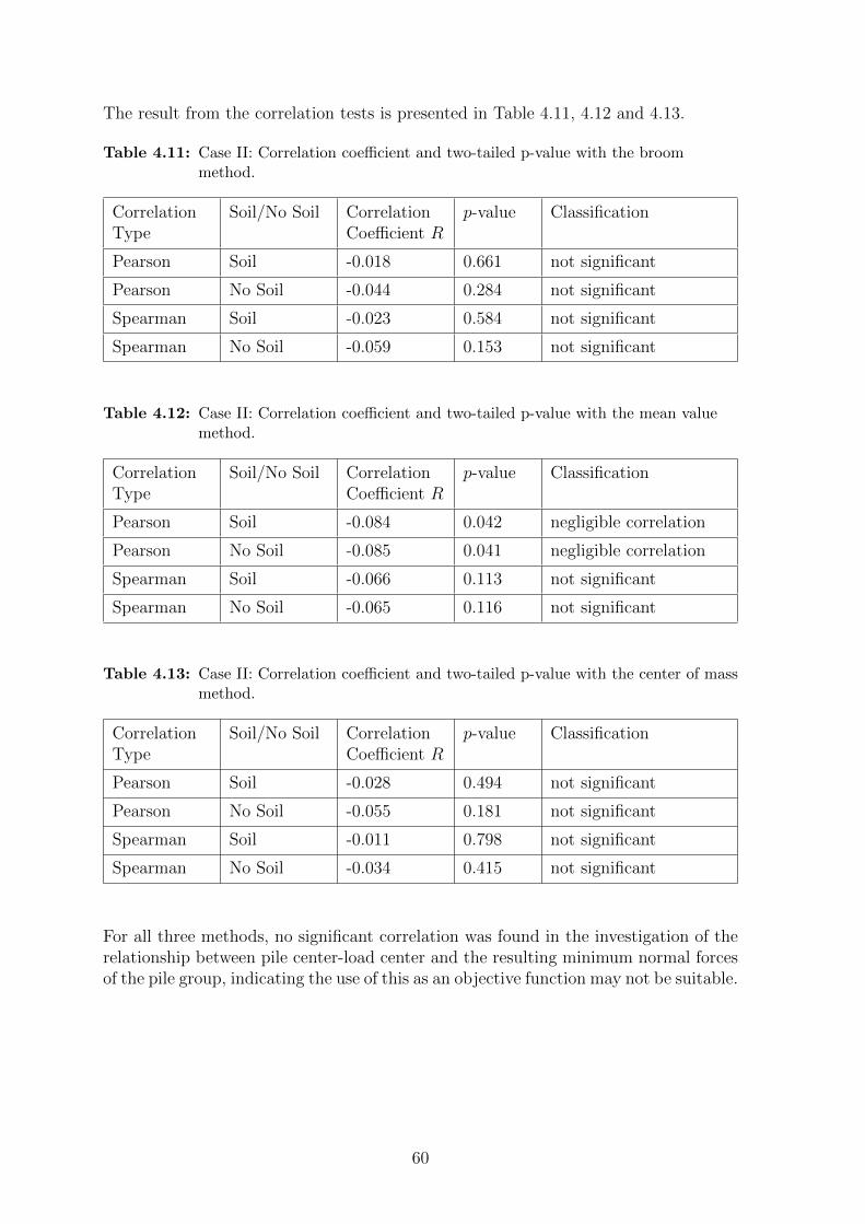
The result from the correlation tests is presented in Table 4.11, 4.12 and 4.13.

Table 4.11: Case II: Correlation coefficient and two-tailed p-value with the broommethod.

CorrelationType



Pearson Soil -0.018 0.661 not significant

Pearson No Soil -0.044 0.284 not significant

Spearman Soil -0.023 0.584 not significant


Table 4.12: Case II: Correlation coefficient and two-tailed p-value with the mean valuemethod.

CorrelationType



Pearson Soil -0.084 0.042 negligible correlation

Pearson No Soil -0.085 0.041 negligible correlation



Table 4.13: Case II: Correlation coefficient and two-tailed p-value with the center of massmethod.

CorrelationType



Pearson Soil -0.028 0.494 not significant

Pearson No Soil -0.055 0.181 not significant



For all three methods, no significant correlation was found in the investigation of therelationship between pile center-load center and the resulting minimum normal forcesof the pile group, indicating the use of this as an objective function may not be suitable.

60

5 Discussion and Conclusion

5.1 Discussion

Finding suitable pile groups for bridges is a time consuming task, as different loadcases have different optimal designs. The aim of this thesis was to automate parts ofthe design process for pile groups. A program generating and evaluating random pilegroups was developed and tested on four cases.

The method for analyzing the pile groups included many simplifications. Firstly, thesoil surrounding the piles was assumed to be homogeneous, i.e. only one type of soilcan be implemented in one analysis. It may not be obvious what layer of soil is decisiveand how to choose soil parameters that are on the safe side, but not overly conservative.Secondly, the frame analysis method does not predict the behaviour of the piles in anexact manner. It assumes an infinitely stiff pile cap and the connection to the pilecap can only be simply supported or moment stiff, whereas the reality is somewherein between. The lateral resistance of the soil was considered by the use of two simplebeam models, the Winkler model and a moment stiff connection at a fictitious length.However, the simplifications for the soil and the structure are reasonable for the scopeof this project - to quickly be able to suggest reasonable, preliminary pile groups.

Calculations with lateral resistance of the soil resulted in less extreme normal forces butlarger shear forces and moments, as expected. For the simulated pile groups in the casestudies, the normal forces were governing the design, meaning that the calculationswithout lateral resistance of the soil were most relevant for the result of the pile grouparrangements. This agrees with indications by designers. However, the differencesbetween calculations with and without soil were small for all cases except Case III.This indicates that some designs are more susceptible to assumptions concerning thesoil than others. There may be cases with high lateral resistance from the soil, thatinduce large governing bending moments in the piles. None of the cases studied hadfriction soil, which may give other results.

Evaluating pile groups both with and without lateral resistance, may not have been thebest approach to investigate whether a Monte Carlo-simulation can facilitate pile grouparrangement. To get more pronounced results the simulation should have been carriedout only with the same assumption about the soil as the existing design. The curiosityabout the influence of the lateral resistance of the soil and the new requirementsfrom Trafikverket, led to a multifaceted project, but also to results that were hard tointerpret.

The developed program does not perform a perfect optimization, but is rather a power-ful, simple tool for arranging pile groups in preliminary design. There are many op-timization algorithms that may have produced more theoretically optimal pile groups.The drawback of Monte Carlo-simulations is the need for a high number of realiza-

61

tions. In pile groups with few piles, it may be more appropriate to test all possiblecombinations, instead of simulating the design variables randomly. Even though theprogram is iterating automatically, there is a need for manual calibration wheneverapplying the program on a new case. This includes how to restrict the options forrotations and inclinations, if and how to apply symmetry restrictions, how many pilegroups to generate, etc. The calibration issues can also be seen as an advantage asthe designer can implement her specific requirements. Once the program is calibrated,the simulation takes a few minutes to an hour, depending on the complexity and thenumber of generated pile groups.

The optimization is driven by an objective function, and the choice of objective func-tion obviously impacts the results. The chosen objective function was to minimize thedifference between maximum and minimum normal forces, with the purpose to dis-tribute forces evenly in the pile group. Although the forces became evenly distributedbetween the piles, the objective function did not assure that the generated sectionforces had any margins to the capacity of the pile group. From one point of view,it may be positive to utilize the capacity of the piles as much as possible. On theother hand, the pile group should be designed with a safety margin due to installationdeviations. Other possible objective functions could be to minimize maximum normalforce or to maximize minimum normal force. These objective functions, including thechosen one, evaluate the pile group based on the result for the critical pile in the pilegroup. This seems reasonable as the pile group is not stronger than its weakest pile.On the other hand, it is a parallel system, meaning that failure of one pile may notlead to overall failure. The weakest link assumption is strictly only relevant for seriessystems, like a chain with links. For minimum normal forces, it may be interesting toevaluate the number of piles that are in tension, rather than only the critical pile. Itis not obvious whether a few piles with large tension forces or many piles with minortension forces is most problematic. Tension anchoring a pile is time consuming andan economical loss, irrespective of the size of the tension force. The number of tensionanchored piles could then be a better indicator of the adequacy of the pile group.

Tension should generally be avoided but in some cases when conditions are favourable,ensuring sufficient tensile capacity is not a problem. This depends on, for example, thetype of soil, the self-weight of the piles and what requirements the project owner has.Another approach is to rely on the resistance of the remaining piles, assuming that thepile in tension does not contribute to the resistance, and that the load is redistributed.If the tensile capacity cannot be verified, arranging the pile group unsymmetrical orincreasing the size of the pile cap may solve the problem. A bigger pile cap allowsfor a more flexible arrangement (implemented in the simulation) and results in largervertical forces from self-weight (must be manually adjusted as input data).

The developed program cannot assure that there are no collisions between the pilesbelow and above ground. This is a general problem for all the case studies. The riskfor collisions is in some cases obvious to assess by inspecting the pile plot visually, andrequire further investigation in other cases. Also, in some of the cases the piles areleaning towards or parallel with each other, meaning that the minimum pile distanceof 0.8 meter is not valid. This issue could be interesting for future studies.

For some cases, the random pile group generator produced pile groups with less number

62

of piles than the reference pile groups. There is not only a reduction of piles, thetension forces also seems to be better. An explanation may be that the applied verticalforces are distributed among fewer piles, resulting in larger compression forces. Thereduction of piles is a great success from both a material and an economical point ofview. However, it is important to keep in mind that the pile group should also bedesigned according to other limit states and the risk for eliminated piles. A pile groupwith fewer number of piles may be less redundant.

To make use of the location of the pile center seems in theory like a logical methodto design pile groups, but in practice several problems arise. It is not obvious howa mathematical model should be created to reflect the reality accurately. Three cal-culation methods for the load center have been performed, the broom method, themean value method and the center of mass method. Only the mean value method forCase I proved low significant correlation for the distance between the pile center-loadcenter and the tension forces in the pile group. All other correlation test showed nosignificant correlation. The explanation for these results may be found in the methodsused for the load center, as they have not been possible to verify.

All three methods require that all load cases are used and that no one has been elim-inated due to, for example, symmetry reasons, otherwise the load center is misplaced.The eccentricities are calculated as a ratio between moment and force, and an infinitesmall force does therefore result in an infinite large eccentricity that may not be rel-evant. The broom method and the mean value method value all eccentricities equally,which may not be reasonable. None of the methods did identify the critical load casesthat generate the worst pile forces. Elaborating with the load center calculations leftus with many questions. Is it relevant to calculate a pile center based on only criticalload cases? Should all load cases have equal value?

Using non-verified methods makes it hard to draw conclusions from the results. If themethods are accurate, there is no reason to minimize the distance between the loadcenter and pile center, as it does not correlate with the resulting minimum normalforces. Irrespective of the validity of the load center calculations, we argue that eval-uating pile groups directly by their section forces is a better way than by using thedistance load center-pile center, especially when using an automatic generating pilegroup program.

5.2 Conclusion

To summarize, the thesis concludes that:

• An optimization program can facilitate the preliminary design of pile groups byautomatizing the iterative task to arrange pile groups suitable for a large numberof load cases. The process still requires some manual surveillance, for example tocalibrate the input data and evaluate the feasibility of the generated pile groups.

• The methods used for investigating the correlation between the distance betweenpile center and load center and resulting tension forces were non-verified. How-

63

ever, the results indicate that the concept may not be suitable as an objectivefunction.

• To facilitate the work at the building site, it is important to account for practicalaspects at an early stage. Robustness, simplicity and limiting the inclinationof the piles, are important aspects according to contractors. For a successfulpile group project, communication between the designer and the contractor isencouraged.

• For the cases studied, calculations without lateral resistance of the soil weredecisive, which is in line with the approach that traditionally has been commonpractice for pile group design. Nevertheless, Trafikverket requires calculationswith lateral resistance of the soil.

64

Bibliography

Alheid, Peter (Mar. 2020). “Questions about practical requirements on a pile group.”Phone Interview.

Bergdahl, Ulf, Bo S. Malmborg and Svensk byggtjanst (1993). Plattgrundlaggning.Svensk byggtjanst. isbn: 9173326623.

Berntsson, Anders (Apr. 2020). “Questions about practical requirements on a pilegroup.” Phone Interview.

Blomqvist, Erik (Mar. 2020). “Questions about practical requirements on a pile group.”Phone Interview.

Bredenberg, Hakan and Bengt Broms (1978). Palgrupper med sidomotstand och inspanning.Rapport / Palkommissionen: 54.

Christensen, Peter W., Anders Klarbring and G. M. L. Gladwell (2008). An introduc-tion to structural optimization. Solid Mechanics and Its Applications: 153. SpringerNetherlands. isbn: 9781402086656.

Das, Braja M. (2002). Principles of geotechnical engineering. Wadsworth Group. isbn:0-534-38742-X.

Eurocode Software AB (2017). caeEC701 Rymdpalgrupp - Anvandarmanual. Rev C.

Hercules Grundlaggning (2018). Betongpaleboken. Anvisningar for projektering, designoch kontroll. 2nd ed. Hercules Grundlaggning AB.

Olsson, Connie, Goran Holm and Svensk byggtjanst (1993). Palgrundlaggning. Svenskbyggtjanst. isbn: 9173326631.

Stal, Torbjorn (1984). Handboken Bygg. Liber forlag. isbn: 9138060779.

Svahn, Per-Ola and Claes Alen (2006). Transversalbelastade palar - statiskt verkningssattoch dimensioneringsanvisningar. Rapport / Palkommissionen: 101.

Sallfors, Goran (2009). Geoteknik: jordmateriallara; jordmekanik. 4th ed.

Thomopoulos, Nick T (2013). Essentials of Monte Carlo Simulation. [Elektronisk re-surs] Statistical Methods for Building Simulation Models. Springer New York. isbn:9781461460213.

Trafikverket (2019a). Krav Brobyggande. 3rd ed. TDOK 2019:0204.

65

Trafikverket (2019b). Rad Brobyggande. 3rd ed. TDOK 2019:0203.

– (2019c). Trafikverkets tekniska krav for geokonstruktioner - TK Geo 13. 2nd ed.TDOK 2013:0667.

66

Appendix A

Interview Questions

The questions asked during the telephone interviews are presented below

• What are the most important characteristics of a pile group (except that it hassufficient bearing capacity)?

• What factors during installation affect the design of the pile group? And doesit vary depending on the pile type?

• Does machine constraints have an impact on the design? If yes, how?

• Does safety aspects and working environment affect the design? If yes, how?

• How does the design of the pile group influence time and cost of installation?

67

Appendix B

Verification with Unit Load

69

Figure B.1: Nx = 10 kN

70

Figure B.2: Nz = 100 kN

71

Figure B.3: Mx = 100 kN

72

Appendix C

Case I

Pedestrian Bridge Mid Support

73

Polaren Pål Report

Version 1.0

Report created 2020-05-08 13:33:34 by Frida Liljefors & Linda Johansson

Project Case Study I. Pedestrian Bridge Mid Support.

General input data

Type of analysis Random generetor: symmetry around two axes

Number of pile groups 100000

Pile connection to pile cap Hinged

Pile material Concrete

Cross section pile Quadratic

Diameter/width d 0.27 [m]

Length of pile L 9 [m]

Youngs modulus E 37.3 [GPa]

Shear modulus G 12.0 [GPa]

Pile capacity

Nmax (1) 800.0 [kN]

M (2) 20.0 [kNm]

N (3) 500.0 [kN]

Mmax (4) 30.0 [kNm]

Nmin -30.0 [kN]

Umax 0.067 [m]

Page 1 of 4

Soil parameters

Type of soil Cohesion

Subgrade modulus kd 300.0 [kPa]

Loads [kN/kNm]

Nx Ny Nz Mx My Mz

185.5 -34.9 1681.3 -256.0 -1132.7 0.0

-169.8 -34.9 1608.8 -256.0 812.9 0.0

-116.4 -92.9 1682.5 -671.4 1146.9 0.0

-116.4 92.9 1682.5 671.4 1146.9 0.0

-116.4 -52.8 1285.5 -382.8 1017.8 0.0

-116.4 -52.8 2430.5 -392.5 1283.4 0.0

-116.4 70.3 2106.1 679.4 1236.8 0.0

-116.4 -92.9 2106.1 -679.4 1222.4 0.0

185.5 -34.9 1994.6 -259.0 -1380.5 0.0

-152.9 -89.9 2106.1 -498.9 1432.7 0.0

21.5 -51.9 2430.5 -388.8 96.7 0.0

148.8 -51.9 2430.5 -388.8 -1038.2 0.0

148.8 51.9 2430.5 388.8 -1038.2 0.0

21.5 51.9 2430.5 388.8 96.7 0.0

-0.5 51.9 2430.5 388.8 200.7 0.0

-127.8 51.9 2430.5 388.8 1335.6 0.0

-127.8 -51.9 2430.5 -388.8 1335.6 0.0

-0.5 -51.9 2430.5 -388.8 200.7 0.0

46.8 -89.9 1307.7 -657.2 -79.4 0.0

173.9 -89.9 1307.7 -657.2 -1035.4 0.0

173.9 89.9 1307.7 657.2 -1035.4 0.0

46.8 89.9 1307.7 657.2 -79.4 0.0

-86.2 89.9 1307.7 657.2 878.8 0.0

-158.2 89.9 1307.7 657.2 1170.4 0.0

-158.2 -89.9 1307.7 -657.2 1170.4 0.0

-86.2 -89.9 1307.7 -657.2 878.8 0.0

101.9 -67.3 1875.8 -663.6 -662.6 0.0

185.5 34.9 1994.6 259.0 -1380.5 0.0

101.9 67.3 1875.8 663.6 -662.6 0.0

-25.8 67.3 2106.1 667.2 372.4 0.0

-152.9 67.3 2106.1 667.2 1432.7 0.0

-152.9 -67.3 2106.1 -667.2 1432.7 0.0

Page 2 of 4

-25.8 -67.3 2106.1 -667.2 372.4 0.0

101.9 -89.9 1380.2 -657.29 -654.7 0.0

185.5 -34.9 1306.5 -255.1 -1227.2 0.0

185.5 34.9 1306.5 255.1 -1227.2 0.0

101.9 89.9 1380.2 657.2 -654.7 0.0

-31.0 89.9 1307.7 657.2 238.1 0.0

-152.9 89.9 1380.2 657.2 1290.7 0.0

-152.9 -89.9 1380.2 -657.2 1290.7 0.0

-31.0 -89.9 1307.7 -657.2 238.1 0.0

185.5 -34.9 2104.9 -259.0 -1252.8 0.0

-169.8 -34.9 1943.8 -258.7 854.3 0.0

-116.4 52.8 2430.5 392.5 1283.4 0.0

173.9 -89.9 1307.7 -657.2 -1053.4 0.0

173.9 89.9 1307.7 657.2 -1053.4 0.0

-158.2 89.9 1307.7 657.2 1194.1 0.0

-158.2 -89.9 1307.7 -657.2 1194.1 0.0

Page 3 of 4

Table C.1: Result Case I. Pile plots and section forces for Pile Group 1, 2 and 3.

77

Appendix D

Case II

Pedestrian Bridge Abutment

79

Polaren Pål Report

Version 1.0


Project Case Study II. Pedestrian Bridge Abutment.

General input data

Type of analysis Random generator: symmetry around one axis









Pile capacity

Nmax (1) 800.0 [kN]

M (2) 20.0 [kNm]

N (3) 500.0 [kN]

Mmax (4) 30.0 [kNm]

Nmin -50.0 [kN]

Umax 0.12 [m]

Page 1 of 3

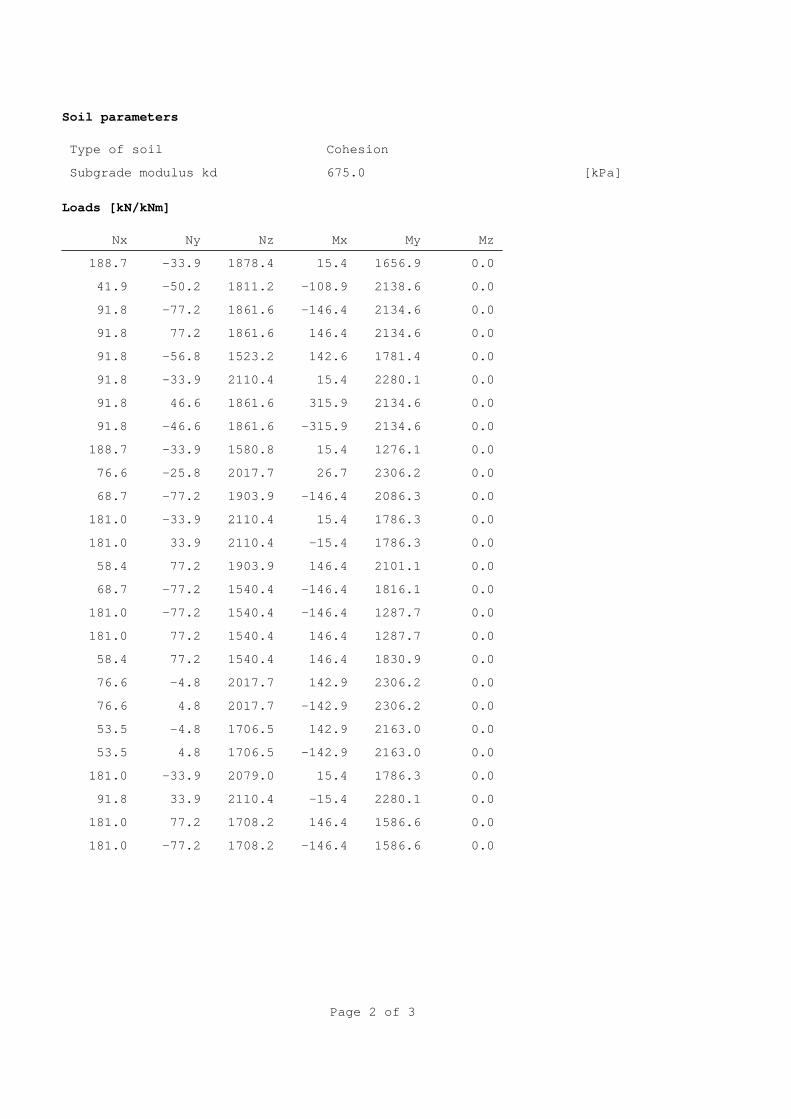
Soil parameters



Loads [kN/kNm]

Nx Ny Nz Mx My Mz

188.7 -33.9 1878.4 15.4 1656.9 0.0

41.9 -50.2 1811.2 -108.9 2138.6 0.0

91.8 -77.2 1861.6 -146.4 2134.6 0.0

91.8 77.2 1861.6 146.4 2134.6 0.0

91.8 -56.8 1523.2 142.6 1781.4 0.0

91.8 -33.9 2110.4 15.4 2280.1 0.0

91.8 46.6 1861.6 315.9 2134.6 0.0

91.8 -46.6 1861.6 -315.9 2134.6 0.0

188.7 -33.9 1580.8 15.4 1276.1 0.0

76.6 -25.8 2017.7 26.7 2306.2 0.0

68.7 -77.2 1903.9 -146.4 2086.3 0.0

181.0 -33.9 2110.4 15.4 1786.3 0.0

181.0 33.9 2110.4 -15.4 1786.3 0.0

58.4 77.2 1903.9 146.4 2101.1 0.0

68.7 -77.2 1540.4 -146.4 1816.1 0.0

181.0 -77.2 1540.4 -146.4 1287.7 0.0

181.0 77.2 1540.4 146.4 1287.7 0.0

58.4 77.2 1540.4 146.4 1830.9 0.0

76.6 -4.8 2017.7 142.9 2306.2 0.0

76.6 4.8 2017.7 -142.9 2306.2 0.0

53.5 -4.8 1706.5 142.9 2163.0 0.0

53.5 4.8 1706.5 -142.9 2163.0 0.0

181.0 -33.9 2079.0 15.4 1786.3 0.0

91.8 33.9 2110.4 -15.4 2280.1 0.0

181.0 77.2 1708.2 146.4 1586.6 0.0

181.0 -77.2 1708.2 -146.4 1586.6 0.0

Page 2 of 3

Reference pile group

x [m] y [m] α [°] β [1:X] L [m]

-2.45 -1.35 270.0 4.0 13.0

-1.5 -1.35 180.0 4.0 13.0

0.5 -1.35 0.0 4.0 13.0

-2.45 1.35 90.0 4.0 13.0

-1.5 1.35 180.0 4.0 13.0

0.5 1.35 0.0 4.0 13.0

Page 3 of 3

Table D.1: Result Case II. Pile plots and section forces for Pile Group 1, 2 and 3.

83

Appendix E

Case III

Road Bridge Mid Support

85

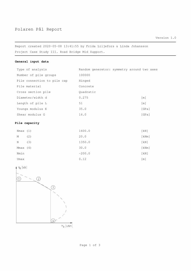
Polaren Pål Report

Version 1.0


Project Case Study III. Road Bridge Mid Support.

General input data

Type of analysis Random generetor: symmetry around two axes









Pile capacity

Nmax (1) 1600.0 [kN]

M (2) 20.0 [kNm]

N (3) 1350.0 [kN]

Mmax (4) 30.0 [kNm]

Nmin -200.0 [kN]

Umax 0.12 [m]

Page 1 of 3

Soil parameters



Loads [kN/kNm]

Nx Ny Nz Mx My Mz

707.0 243.0 21401.0 8492.0 -10016.0 0.0

707.0 243.0 20924.0 9534.0 -9926.0 0.0

1189.0 243.0 18723.0 9317.0 -13158.0 0.0

807.0 243.0 7261.0 4132.0 -8095.0 0.0

807.0 243.0 10692.0 10819.0 -8628.0 0.0

1111.0 243.0 10003.0 3722.0 -11118.0 0.0

763.0 308.0 20292.0 11140.0 -10253.0 0.0

949.0 484.0 19311.0 10993.0 -11487.0 0.0

763.0 308.0 19656.0 12531.0 -10136.0 0.0

1398.0 484.0 16897.0 11773.0 -14514.0 0.0

863.0 308.0 7684.0 4833.0 -8615.0 0.0

1049.0 484.0 7885.0 6566.0 -10116.0 0.0

863.0 308.0 11777.0 13748.0 -9317.0 0.0

1319.0 484.0 10002.0 6202.0 -12808.0 0.0

Page 2 of 3


x [m] y [m] α [°] β [1:X] L [m]

-2.0 -4.5 180.0 8.0 51.0

-2.0 -3.5 180.0 13.0 51.0

-2.0 -2.5 180.0 8.0 51.0

-2.0 2.5 180.0 8.0 51.0

-2.0 3.5 180.0 13.0 51.0

-2.0 4.5 180.0 8.0 51.0

-1.0 -5.75 270.0 8.0 51.0

-1.0 -4.5 180.0 13.0 51.0

-1.0 -3.5 180.0 20.0 51.0

-1.0 -2.5 180.0 13.0 51.0

-1.0 2.5 180.0 13.0 51.0

-1.0 3.5 180.0 20.0 51.0

-1.0 4.5 180.0 13.0 51.0

-1.0 5.75 90.0 8.0 51.0

1.0 -5.75 270.0 8.0 51.0

1.0 -4.5 0.0 13.0 51.0

1.0 -3.5 0.0 20.0 51.0

1.0 -2.5 0.0 13.0 51.0

1.0 2.5 0.0 13.0 51.0

1.0 3.5 0.0 20.0 51.0

1.0 4.5 0.0 13.0 51.0

1.0 5.75 90.0 8.0 51.0

2.0 -4.5 0.0 8.0 51.0

2.0 -3.5 0.0 13.0 51.0

2.0 -2.5 0.0 8.0 51.0

2.0 2.5 0.0 8.0 51.0

2.0 3.5 0.0 13.0 51.0

2.0 4.5 0.0 8.0 51.0

Page 3 of 3

Table E.1: Result Case I. Pile plots and section forces for Pile Group 1, 2 and 3.

89

Appendix F

Case IV

Railway Bridge Abutment

93

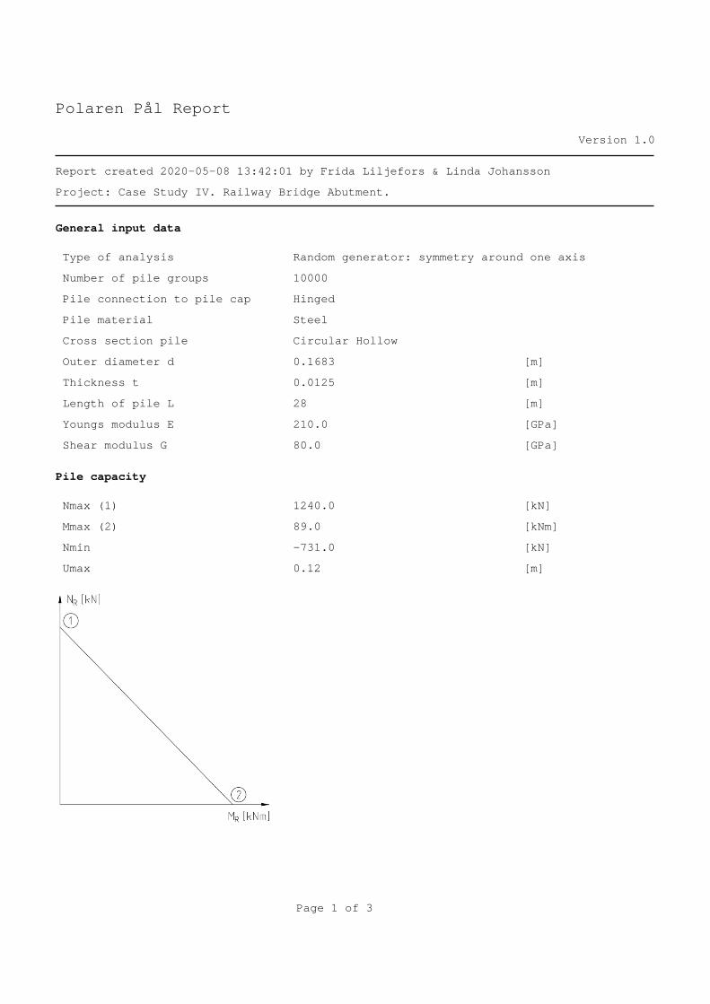
Polaren Pål Report

Version 1.0


Project: Case Study IV. Railway Bridge Abutment.

General input data

Type of analysis Random generator: symmetry around one axis



Pile material Steel

Cross section pile Circular Hollow

Outer diameter d 0.1683 [m]

Thickness t 0.0125 [m]




Pile capacity

Nmax (1) 1240.0 [kN]

Mmax (2) 89.0 [kNm]

Nmin -731.0 [kN]

Umax 0.12 [m]

Page 1 of 3

Soil parameters



Loads [kN/kNm]

Nx Ny Nz Mx My Mz

777.0 -75.0 10109.0 -1316.0 -1436.0 0.0

754.0 -127.0 10109.0 -1641.0 -1399.0 0.0

488.0 -75.0 6964.0 -1316.0 -2261.0 0.0

466.0 -127.0 6964.0 -1641.0 -2225.0 0.0

418.0 -23.0 6123.0 -150.0 -1551.0 0.0

418.0 -23.0 6123.0 -150.0 -1551.0 0.0

731.0 -75.0 10109.0 -1316.0 -1363.0 0.0

746.0 -127.0 10109.0 -1641.0 -1418.0 0.0

746.0 -88.0 9401.0 -1608.0 -1418.0 0.0

717.0 -152.0 9410.0 -2014.0 -1373.0 0.0

470.0 -88.0 7174.0 -1608.0 -2377.0 0.0

441.0 -152.0 7174.0 -2014.0 -2331.0 0.0

381.0 -23.0 6123.0 -150.0 -1488.0 0.0

381.0 -23.0 6123.0 -150.0 -1488.0 0.0

689.0 -88.0 9401.0 -1608.0 -1327.0 0.0

689.0 -88.0 9401.0 -1608.0 -1327.0 0.0

119.0 0.01 6123.0 0.01 -1086.0 0.0

Page 2 of 3


x [m] y [m] α [°] β [1:X] L [m]

2.0 -3.2 0.0 4.0 28.0

2.0 -1.6 0.0 4.0 28.0

2.0 1.6 0.0 4.0 28.0

2.0 3.2 0.0 4.0 28.0

0.55 -3.2 270.0 4.0 28.0

0.55 -2.4 0.0 4.0 28.0

0.55 -0.8 0.0 4.0 28.0

0.55 0.8 0.0 4.0 28.0

0.55 2.4 0.0 4.0 28.0

0.55 3.2 90.0 4.0 28.0

-2.0 -3.2 180.0 4.0 28.0

-2.0 -2.4 270.0 4.0 28.0

-2.0 -1.6 180.0 4.0 28.0

-2.0 1.6 180.0 4.0 28.0

-2.0 2.4 90.0 4.0 28.0

-2.0 3.2 180.0 4.0 28.0

-1.2 -3.2 270.0 4.0 28.0

-1.2 -0.8 180.0 4.0 28.0

-1.2 0.8 180.0 4.0 28.0

-1.2 3.2 90.0 4.0 28.0

Page 3 of 3

Table F.1: Result Case I. Pile plots and section forces for Pile Group 1, 2 and 3.

97

Master Thesis Pile Group Design - lup.lub.lu.se

Documents

Transcript of Master Thesis Pile Group Design - lup.lub.lu.se