Master Thesis - Lu
124
Master Thesis Comparison and Evaluation of Didactic Methods in Numerical Analysis for the Teaching of Cubic Spline Interpolation Abtihal Jaber Chitheer supervised by Prof. Dr. Carmen Ar´ evalo May 17, 2017
Transcript of Master Thesis - Lu

Master Thesis
Comparison and Evaluation of Didactic Methods in NumericalAnalysis for the Teaching of Cubic Spline Interpolation
Abtihal Jaber Chitheer
supervised by Prof. Dr. Carmen Arevalo
May 17, 2017

ii

Lund University
Abstract
Faculty of ScienceCentre for Mathematical Sciences
Numerical analysis
Master in Science
Comparison and Evaluation of Didactic Methods in Numerical Analysis forthe Teaching of Cubic Spline Interpolation
by Abtihal Jaber Chitheer
In mathematical education it is crucial to have a good teaching plan and to execute it correctly.In particular, this is true in the field of numerical analysis. Every teacher has a different styleof teaching. This thesis studies how the basic material of a particular topic in numericalanalysis was developed in four different textbooks. We compare and evaluate this process inorder to achieve a good teaching strategy. The topic we chose for this research is cubic splineinterpolation. Although this topic is a basic one in numerical analysis it may be complicatedfor students to understand. The aim of the thesis is to analyze the effectiveness of differentapproaches of teaching cubic spline interpolation and then use this insight to write our ownchapter. We intend to channel every-day thinking into a more technical/practical presentationof a topic in numerical analysis. The didactic methodology that we use here can be extendedto cover other topics in numerical analysis.

ii

Acknowledgements
I would like to express my gratitude towards my country Iraq for the scholarship. I would liketo thank Lund University for giving me the opportunity to do my master degree. I would liketo thank my supervisor Carmen Arevalo for giving me this opportunity to do my master thesisin the field of numerical analysis and for the guidance and support throughout the process.I would like also to thank the department of Mathematics for feedback and encouragement.Finally I am very grateful for support from my loving family and friends.
iii

iv

Contents
1 Introduction 1
1.1 Aim of the thesis . . . . . . . . . . . . . . . . . . . . . . . . . . . . . . . . . . . 1
1.2 Spline interpolation . . . . . . . . . . . . . . . . . . . . . . . . . . . . . . . . . . 1
1.3 Didactic reflection: . . . . . . . . . . . . . . . . . . . . . . . . . . . . . . . . . . 2
1.4 Additional notes . . . . . . . . . . . . . . . . . . . . . . . . . . . . . . . . . . . 2
2 Analysis of the books 3
2.1 Comparison criteria . . . . . . . . . . . . . . . . . . . . . . . . . . . . . . . . . 3
2.2 Book descriptions . . . . . . . . . . . . . . . . . . . . . . . . . . . . . . . . . . . 4
2.2.1 Book I: Applied Numerical Methods with MATLAB for Engineers andScientists by Steven C. Chapra, 2011. . . . . . . . . . . . . . . . . . . . 4
2.2.1.1 Insertion Point . . . . . . . . . . . . . . . . . . . . . . . . . . . 5
2.2.1.2 Teaching Structure . . . . . . . . . . . . . . . . . . . . . . . . . 11
2.2.1.3 Outcome Procurement . . . . . . . . . . . . . . . . . . . . . . 13
2.2.2 Book II: Numerical Analysis by Timothy Sauer, 2012. . . . . . . . . . . 18
2.2.2.1 Insertion point . . . . . . . . . . . . . . . . . . . . . . . . . . . 20
2.2.2.2 Teaching structure . . . . . . . . . . . . . . . . . . . . . . . . . 21
2.2.2.3 Outcome Procurement . . . . . . . . . . . . . . . . . . . . . . 24
2.2.3 Book III: Numerical Analysis: Mathematics of Scientific Computing, byDavid Kincaid and Ward Cheney, 2002. . . . . . . . . . . . . . . . . . . 24
2.2.3.1 Insertion point . . . . . . . . . . . . . . . . . . . . . . . . . . . 25
2.2.3.2 Teaching structure . . . . . . . . . . . . . . . . . . . . . . . . . 28
2.2.3.3 Outcome Procurement . . . . . . . . . . . . . . . . . . . . . . 31
2.2.4 Book IV: Applied Numerical Analysis Using MATLAB by Laurene V.Fausett, 2008. . . . . . . . . . . . . . . . . . . . . . . . . . . . . . . . . . 32
2.2.4.1 Insertion Point . . . . . . . . . . . . . . . . . . . . . . . . . . . 34
2.2.4.2 Teaching Structure . . . . . . . . . . . . . . . . . . . . . . . . . 38
2.2.4.3 Outcome Procurement . . . . . . . . . . . . . . . . . . . . . . 41
3 Comparison and Evaluation 43
3.1 Points in need of revision . . . . . . . . . . . . . . . . . . . . . . . . . . . . . . 71
4 Suggestion of presentation 77
X.1 Interpolation in general . . . . . . . . . . . . . . . . . . . . . . . . . . . . . . . 80
X.1.1 What is interpolation? . . . . . . . . . . . . . . . . . . . . . . . . . . . . 80
v

vi CONTENTS
X.1.2 Why do we study interpolation? . . . . . . . . . . . . . . . . . . . . . . 80X.1.3 Types of interpolating functions . . . . . . . . . . . . . . . . . . . . . . 83
X.2 Polynomial Interpolation . . . . . . . . . . . . . . . . . . . . . . . . . . . . . . . 83X.2.1 Monomial Basis . . . . . . . . . . . . . . . . . . . . . . . . . . . . . . . . 84X.2.2 Lagrange Basis . . . . . . . . . . . . . . . . . . . . . . . . . . . . . . . . 85X.2.3 Runge’s Phenomenon . . . . . . . . . . . . . . . . . . . . . . . . . . . . 89
X.3 Piecewise polynomial Interpolation . . . . . . . . . . . . . . . . . . . . . . . . . 92X.3.1 Piecewise linear Interpolation . . . . . . . . . . . . . . . . . . . . . . . . 92X.3.2 Quadratic Spline Interpolation . . . . . . . . . . . . . . . . . . . . . . . 94X.3.3 Cubic Spline Interpolation . . . . . . . . . . . . . . . . . . . . . . . . . . 98
X.3.3.1 What are the conditions to determine an interpolation cubicspline? . . . . . . . . . . . . . . . . . . . . . . . . . . . . . . . 98
X.3.3.2 Construction of an interpolatory cubic spline. . . . . . . . . . . 101X.3.3.3 Why cubic spline interpolation? . . . . . . . . . . . . . . . . . 107X.3.3.4 Discussion . . . . . . . . . . . . . . . . . . . . . . . . . . . . . 108
X.3.4 A historical fact of cubic splines interpolation. . . . . . . . . . . . . . . 108
5 Conclusion and Future Work 111
A Example (Table lookup): 115

Chapter 1
Introduction
Many problems in mathematics can be presented in several different ways, but all lead us tothe same results. Most problems are complex problems, that might be difficult for students tounderstand. When I was working in Iraq as a mathematics teacher during the years of 2009-2013 I realized that different ways of teaching will affect the students’ level of understanding.Piecewise polynomial interpolation is one topic that students find especially difficult to un-derstand, so we would like to find didactic strategies for teaching this subject. The topic ofcubic spline interpolation is a basic topic in the course of numerical analysis and yet studentshave difficulties in following the process of the construction of a cubic spline based on theconditions a spline must satisfy.
These problems are solved numerically, usually with the help of computers and thus learninghow to program this process is also a skill students must develop.
1.1 Aim of the thesis
A mathematical object or concept can be introduced by different sets of equivalent definitionsand examples. One fundamental question in this context is that of what teaching methodto use. Reading several books on a common topic makes one realize how different similarteachings can be, in style and requirements towards a student. Our goal, in this work ofcomparison, is to analyze the effectiveness of different approaches and teachings of someparticular topics through different course materials, and how to compare and decide betweendifferent books with future work in Iraq in mind.
Eventually, the aim of this work is to channel every-day thinking towards a more technical-practical thinking at an earlier stage so that, as a teacher, one can get the expected resultsfrom the teaching of a particular topic.
1.2 Spline interpolation
Here we chose to focus on the teaching of spline interpolation. The choice of this topic hastwo main motivations. First of all, it is one of the basics of numerical analysis. Using anexample that is easily understandable by undergraduate students of mathematicians makesthe point of the thesis easier to illustrate. Secondly, there are many differences in views and
1

2 CHAPTER 1. INTRODUCTION
the teaching of this subject, and the study of these differences helps to reach the goal of thisthesis. Diversity in teaching strategies gives us tools to reach our goal.
1.3 Didactic reflection:
Variation theory of learning was developed by Ference Marton of the University of Gothenburgin 1997. This theory says that for a teacher to be able to help a student understand atopic, the teacher must first identify the critical aspects of the topic. Once this is done, byvarying one aspect while keeping other aspects fixed, the student will learn by observing thedifferences. Variation theory can be interpreted as “how the same thing or the same situationcan be seen, experienced or understood in a limited number of qualitatively different ways”[Maghdid, 2016]. For example, we apply variation theory when we propose several problemsthat can be solved with the same technique, or when we have one example that can be solvedin several different ways. In our development of a chapter for the teaching of cubic splineinterpolation we will apply this strategy to try to reach a successful didactics method.
1.4 Additional notes
The four books we have chosen to work with are well-known and used often in the teachingof numerical analysis.
Our goal is not to describe one perfect way of teaching, but to hierichize the methods andteaching strategies by their efficiency.
Any student with basic knowledge of numerical analysis can read this thesis. As we havestated before, our point is not the mathematical aspects but the didactics. Therefore, abasic knowledge is enough and necessary in order to understand most of our points andexamples, which will only be clearer if the reader has studied spline interpolation in thepast. Furthermore, any person interested in the teaching of mathematics may be interested inreading this work, as successful teaching results from a critical point of view, and especiallya self-critical one.
I am a former student of the Department of Mathematics at Mustansiriya University,Iraq, where I have obtained a Bachelor’s degree in theoretical mathematics. I was thenemployed as a mathematics teacher in the schools Fatima Zahra and Ishtar, where I wasoften confronted with student complains about the lack of easy accessibility to concepts intheoretical mathematics. Their abstract aspect and the specificity of their applications madestudents unable to identify their own errors when obtaining incorrect solutions to a problem.I therefore got very drawn into constructing proofs and solutions that were more interestingand transparent. I aspire to develop a better teaching method, more comfortable for bothteachers and students, by, for example, privileging illustration over expansive calculations.

Chapter 2
Analysis of four differentapproaches to the teaching ofsplines
In this thesis I have compared the presentation of the topic cubic splines from four differentNumerical Analysis books intended to be used as textbooks in regular undergraduate courses.
2.1 Comparison criteria
The four numerical analysis books present the topic under study in considerably differentways. In order to understand their similarities, differences, weaknesses and strengths, we willuse the following key points as comparison criteria: insertion point, teaching structure, andoutcome procurement. Analysis of the structure of teaching is a logical requirement to explaindifferent effectiveness in teaching outcome. To understand the way an author argues we haveto take specific study and comparison criteria. These key points are as follows:
1. Insertion point : Here we will focus on how the author introduces the concept of cubicsplines. We will study the ways in which the authors motivate and direct the reader tocubic splines. For example, how was the presentation initiated? What are the differenttypes of interpolation that are described before starting the cubic spline section? Howis the previous material on interpolation used to connect to this subject?
2. Teaching structure: This part is divided into two subsections. Firstly, we touch on theIntroduction process. What are the key points in the initial presentation of cubic splines?What was the strategy for developing the important concepts in the topic? Secondly,we look at at the elaboration process. In this part we study how the authors expandon the topic, developing each point so that there is a line of development throughout.For example, how is the derivation of cubic splines done? How many end conditions arementioned? Were there any Theorems mentioned or were the explanations of a moreinformal type?
3. Outcome procurement : This part deals with the conclusions of the presentation of thesubject. For example, were there examples and applications that clarified the concept
3

4 CHAPTER 2. ANALYSIS OF THE BOOKS
Insertion Point Teaching Structure
Introduction
Outcome
Procurement
Comparison criteria
Elaboration
3 2 1
2.1
2.2
Figure 2.1: Scheme of the comparison criteria keys
of cubic splines? Are there exercises that allow the reader to test his understanding ofcubic splines? Were there any summaries at the end of the presentation?
Using these criteria we will be able to study and analyze each book in a systematic mannerso that we can use this knowledge in the next chapter to compare the four books and evaluatetheir didactic methods. The comparison will be made in the form of questions and answers,and this will allow us to go on to the evaluation of the books. Finally, using the results ofprevious chapters we will come with our conclusion and suggest a didactic method for thistopic.
The tables and plots shown in the presentation of the books in the following subsectionswere taken directly from the books themselves. The last section of the thesis, the Appendix,displays a copy of the chapters or sections that have been mentioned in this thesis. This wasdone in order to make it easier for the reader to compare the original versions with the thesis.
2.2 Book descriptions
The analysis of each book will start with a schematic representation of how the subject of cubicsplines is presented and developed. This will be done by using the key comparison criteriamentioned before, that is, insertion point, teaching structure, and outcome procurement. Wewill then go on to explain each section in detail.
2.2.1 Book I: Applied Numerical Methods with MATLAB for Engineersand Scientists by Steven C. Chapra, 2011.
Steven C. Chapra is professor at the Department of Civil and Environmental Engineering atTufts University in Massachusetts, U.S.A. He specializes in environmental engineering.
This book focuses on applied numerical analysis using MATLAB. The book can be usedfor teaching at a basic level and at a more advanced level, and Chapra’s book is widely used

2.2. BOOK DESCRIPTIONS 5
Figure 2.2: Steven C.Chapra, author of the book Applied Numerical Methods with MATLABfor Engineer and Scientists, 2011.
as textbook in different countries. For example, Florida University ([University of Florida,2009]) in the United States has been using this book for the course Introduction of NumericalMethods of Engineering Analysis. McMaster University in Canada recently used Chapra’sbook as textbook in the course Computer Engineering 3 SK3 Numerical Analysis ([McMasterUniversity, 2014]), and Hacettepe University in Turkey uses this book as textbook in thecourse Numerical Analysis with MATLAB ([Hacettepe Universitesi, 2017]). In Italy, it is alsoused for the course Numerical Methods at the online Universita Telematica InternazionaleUNINETTUNO. The topic of cubic splines is a 10-page section in the chapter Splines andPiecewise Interpolation. Cubic Splines is mentioned as the last type of spline interpolant andthis section also includes a primer on piecewise interpolation in MATLAB.
2.2.1.1 Insertion Point
The chapter titled Splines and Piecewise Interpolation in Chapra’s book is grounded on itspreceding chapter, Polynomial Interpolation, where Runge’s function was introduced as anexample of the dangers of higher-order polynomial interpolation. The motivation starts bymentioning the problems observed in the previous chapter with higher degree polynomials,but without any reference to Runge’s function example. In addition, the author proposesan alternative solution to this problem by using piecewise lower order polynomials (splinefunctions).
The chapter on splines and polynomial interpolation is opened with an example. When afunction varies sharply at a point, interpolation polynomials of high degree induce undesiredoscillations. This problem is illustrated in Figure 2.4. A linear 3-piece polynomial, as shownin (d), does a much better job that the polynomials of degree 3, 5 and 7, shown in (a, b, c).
The notion of splines is introduced as piecewise lower-order interpolating polynomials,and they are suggested as an alternative to higher-order polynomials when the function tointerpolate has local, abrupt changes.
After presenting the reader with a motivation to study splines, the author gives a historicalaccount of spline construction. In order to “draw smooth curves through a set of points” whena plan for some construction was drafted, a thin, flexible strip (called a spline) was used. Theauthor points to Figure 2.5 to illustrate that the data point (pins) are “interpolated” by

6 CHAPTER 2. ANALYSIS OF THE BOOKS
Book I
Chapra
Natural Splines end
conditions
Quadratic Splines
Introduction to Splines
Linear Splines
1.1
1.2
1.3
Piecewise
Interpolation in
MATLAB
Table lookup
1.2.1
1.5
Insertion Point
Derivation of Cubic
Splines
Clamped end
condition
Not-a-Knot end
condition
1.4.2
End Conditions
1.4.3
Cubic Splines
General formula and
properties
Teaching
Structure
1.4
Elaboration
End conditions
Introduction
Outcome
Procurement
Computer
codes
Examples
Exercises
Case Study
Figure 2.3: Schematic content and organization of Chapter 18, ”Splines and Piecewise Inter-polation” in Chapra’s book [Chapra, 2011].

2.2. BOOK DESCRIPTIONS 7
Figure 2.4: Spline vs. high-order interpolation ([Chapra, 2011], p. 430).

8 CHAPTER 2. ANALYSIS OF THE BOOKS
Figure 2.5: Illustration of an early use of splines to construct smooth curves passing throughpre-defined points (Chapra [2011], p. 431).
Figure 2.6: This figure displays the notation used to derive splines (Chapra [2011], p. 432).
smooth curves as the strip goes through the pins. In fact, the author asserts that these curvesare in fact cubic splines.
At the end of his introductory section, the author gives an overview of the topics that hewill discuss in the remainder of the chapter.
Linear Splines
The section on linear splines starts with a detailed description of the notation, as portrayedin Figure 2.6.
Firstly, the reader is asked to observe that n distinct data points generate n−1 intervals. Itis then shown that for each interval i there is a spline function Si(x), and that a linear splinehas a straight line connection between the two end points of the intervals. Thus, it is easyto formulate the equations for these splines. Then, the practical aspect of this formulation

2.2. BOOK DESCRIPTIONS 9
Figure 2.7: (a) Linear spline, (b) Quadratic spline, (c) Cubic spline, with a cubic interpolationpolynomial, ([Chapra, 2011, p. 433].
is exposed: they can be used to evaluate the function at any point in the interval containingthe data points. The author explains that there are two steps in doing so: (1) locate thesubinterval where the point lies, and (2) use the appropriate equation to evaluate the spline.An example is given to illustrate these steps.
Chapra points out that using linear splines is equivalent to “using Newton’s first-orderpolynomial to interpolate within each interval”. An example shows the first-order spline, thesecond-order spline, and the cubic spline interpolations of four data points (Figure 2.7). Theaim of Figure 2.7, is to demonstrate that the same data points can be interpolated by splinesof different orders: a linear spline, a quadratic spline, and a cubic spline, and that the resultingsplines will yield different function evaluations. It also introduces the concept of smoothnessof a curve, and its relation to its derivatives.
Here another new concept is introduced: a knot is defined as a data point where two splinepieces meet. The author indicates the main disadvantages of linear splines:
1. First-order splines are not smooth.
2. The slope changes abruptly where the spline segments meet (knots).
3. The first derivative of the function is discontinuous at these specific points.

10 CHAPTER 2. ANALYSIS OF THE BOOKS
Figure 2.8: Table (17.7) from the previous chapter, showing air density at different tempera-tures (Chapra [2011], p. 406).
The disadvantage of the non-smoothness of linear splines is a motivation why it is impor-tant to consider higher-order splines. Nevertheless, the author states that linear splines areimportant in their own right, and gives an example of their usefulness.
Table Lookup
Chapra uses the example of a table lookup to show why linear spline interpolation may beuseful. The idea is to interpolate values from a table of independent and dependent variables.“For example, suppose that you would like to set up an M-file that would use linear interpo-lation”, if programming in MATLAB, with specific data that you have as a table, for exampleTable 2.8.
Given such a table, to perform a linear interpolation at a particular value of the independentvariable, the subinterval containing the required value must be found. The action of findingthe appropriate values in the table is called table lookup. Here the author explains in detailhow to construct a Matlab file that does the interpolation task. He describes the process intwo steps:
1. search of the interval where the independent variable is located, and
2. linear interpolation.
The first step is described in detail, and two different types of search are presented: a sequentialsearch, for a small set of data points, and a binary search, for large sets of data.
The next section takes on the aspect of the continuity of the derivatives of the interpolatingfunction.
Quadratic Splines
The author starts this section by claiming that in order to have n-the continuous derivatives, aspline must be of degree n+1 or higher. Then he asserts that the most frequently used splinesare the cubic ones, because higher derivative discontinuities at the knots in most cases cannot

2.2. BOOK DESCRIPTIONS 11
be observed visually. Even though the author’s aim is to discuss cubic splines, he chooses togo through the derivation of quadratic splines because this derivation is less complicated.
The derivation of quadratic splines is done in detail in order to show what are the importantpoints that must be taken into account. It starts by giving the general form of each splinesegment as a quadratic polynomial centered at the starting point of each subinterval,
Si(x) = ai + bi(x− xi) + ci(x− xi)2 (2.1)
Then it proceeds to count the number of intervals, equations, and unknowns, which mustcorrespond to the number of coefficients of the spline. Finally, it gives the conditions thatmust be satisfied by the unknowns. These conditions are continuity conditions, interpola-tion conditions and end conditions. By counting the number of continuity and interpolationconditions, it is clear that there must be one end condition so that the number of equations(conditions) equals the number of unknowns.
Finally, an example is given (Example 18.2 in the book) to illustrate this construction.This example uses the same data as the previous example in the section for linear splines. Inaddition, it refers the reader to Figure 2.7, where (b) shows this quadratic spline, and pointsto the fact that a straight line connects the first two data points due to the end condition,and also that the curve for the last interval swings too high. These observations serve as amotivation to study cubic splines, as they do not exhibit this undesired behaviour.
2.2.1.2 Teaching Structure
This section is divided into two parts. Firstly, the Presentation part refers to the introductionof the basic material defining cubic splines. Secondly, the Elaboration part contains furtherdetails about cubic splines.
Introduction
The author starts by restating the disadvantages of using linear or quadratic splines, andthen states that higher degree splines tend to exhibit inherent instabilities, while cubic splines“exhibit the desired appearance of smoothness” while providing the simplest representation.The steps in which the author displays cubic splines follow the lines of his exposition forquadratic splines:
1. General form of cubic splines.
Si(x) = ai + bi(x− xi) + ci(x− xi)2 + di(x− xi)3 (2.2)
2. Number of intervals, unknowns, and continuity and interpolation conditions.
3. Calculation of the number of end conditions that need to be added, and what formula-tions they can have.
4. Enforcement of the continuity and interpolation conditions.
5. Discussion of the several options for end conditions. One type of end condition is,for example, the conditions for a natural spline, which can be observed in Figure 2.5.Additionally, to complement the choice of several options, the author adds two moreoptions of end conditions which are described in Section 18.4.2 of the book.

12 CHAPTER 2. ANALYSIS OF THE BOOKS
6. Enforcement of the end conditions.
In the next section we present the details of the derivation of cubic splines in Chapra’sbook.
Elaboration
There are two main issues in the construction of cubic splines. Firstly, the derivation of cubicsplines from the continuity and interpolation conditions. Secondly, the enforcement of endconditions.
Derivation of Cubic Splines
A major reason for the introduction and derivation of quadratic splines was to pave the wayto the derivation of cubic splines. Correspondingly, also here the number of conditions andthe number of unknowns are determined, and it is shown that two additional end conditionsare required. The construction of cubic splines is demonstrated step by step.
1. The formula for a cubic spline (third-order polynomial for each interval between knots)is given. This formula is centered around the initial point of each subinterval.
2. The interpolation and continuity conditions for the cubic spline at the knots are enforced.
3. The continuity conditions for the first derivative of the cubic spline at the knots areenforced.
4. The continuity conditions for the second derivative of the cubic spline at the knots areenforced.
5. The result obtained in the previous steps are substituted into the original formula,yielding a set of equations containing only the unknowns corresponding to the coefficientsof the quadratic terms of the spline sections. These equations hold for all the internalknots.
6. The two end conditions are added to the system. As an example, the conditions takenare those for a natural spline, i.e., that the second derivative of the spline is equal tozero at the endpoints.
7. The linear system is shown in a matrix-vector form, showing that the system matrix istridiagonal.
Finally, an example of the construction of a natural cubic spline is shown in [p. 442] ofChapra’s book ([Chapra, 2011]). The author provides the same data that was used for linearand quadratic splines, and the results are displayed in Figure 2.7.
The first type of end conditions applied to cubic splines resulted in natural splines. In thenext section, the author describes other end conditions.
End Conditions

2.2. BOOK DESCRIPTIONS 13
Figure 2.9: How to specify different end conditions (Chapra [2011], p.443 ).
I: Natural End Condition
As described earlier, a natural spline is defined by requiring that the second derivatives atthe two endpoints are equal to zero. This type of spline results when the drafting spline isallowed to behave naturally, without constraining it at its endpoints.
II: Clamped End Condition
Clamped splines result when a drafting spline is clamped at its ends. The first derivative isspecified at the two ends.
III: Not-a-Knot End Condition
This condition implies that the third derivative is required to be continuous at the secondand the next-to-last knots. Because the spline segments are cubic polynomials, this conditionimplies that the first and second segments are a single polynomial, and so are the last andnext-to-last segments. Thus, these knots are not true knots any longer.
Table 2.9 shows how to modify the first and last equations in order to construct natural,clamped and not-a-knot splines. Figure 2.10 shows the different end conditions by using thesame example that was mentioned last section.
2.2.1.3 Outcome Procurement
In the next section the author describes how the user can take advantage of some of Matlab’sbuilt-in functions for piecewise interpolation. Two problems are solved as examples. Somesnippets of code are given, and the results are plotted.
Piecewise Interpolation in MATLAB
The author introduces two possible functions for piecewise interpolation.

14 CHAPTER 2. ANALYSIS OF THE BOOKS
Figure 2.10: Using the data of the previous example, splines with natural, clamped and not-a-knot end conditions are plotted (Chapra [2011], p. 444).

2.2. BOOK DESCRIPTIONS 15
Figure 2.11: Runge’s function with nine data points constructed in MATLAB by using a“not-a-knot” end condition ([Chapra, 2011, p. 445]).

16 CHAPTER 2. ANALYSIS OF THE BOOKS
Figure 2.12: Runge’s function with nine data points constructed in MATLAB by using aclamped end condition (Chapra [2011], p. 446).

2.2. BOOK DESCRIPTIONS 17
Figure 2.13: Discrete data fitted with (a) a first degree spline (b) a zero degree spline (c) astandard spline (d) an Hermite spline (Chapra [2011], p. 448).

18 CHAPTER 2. ANALYSIS OF THE BOOKS
Figure 2.14: Timothy Sauer, author of the book Numerical Analysis, 2012.
1. The spline function implements cubic spline interpolation. The author describes thesyntax and explains how to choose different end conditions. He then uses Runge’sfunction, already mentioned in the previous chapter (example 17.7), to show how theuse of different cubic splines remove the oscillations caused by the Runge phenomenon.The results using different end conditions are presented in Figures 2.11 and 2.12.
2. The function interp1 implements spline and Hermite interpolation and also other typesof piecewise interpolation. Here is an easy way to implement “a number of different typesof piecewise one-dimensional interpolations” with a given general formula. There arefour different optional functions: nearest (for nearest neighbor interpolation), linear(for linear interpolation), spline (for piecewise cubic spline), and pchip (for piecewisecubic Hermite interpolation). Finally, an example is presented to illustrate the trade-offsof using interp1, as shown in Figure 2.13.
After having presented the subject of cubic splines in detail the author solves a particularreal-life heat transfer problem by using cubic splines. The solution is presented in great detail([Chapra, 2011], p. 452–456).
2.2.2 Book II: Numerical Analysis by Timothy Sauer, 2012.
Timothy Sauer is professor of mathematics at George Mason University. He specializes indynamical systems.
This book is intended for students of engineering, science, mathematics, and computerscience. The book offers an introductory level with some more advanced level topics, and usesMATLAB for its computer examples. Sauer’s book is used as textbook in many countries.For example, Washington State University used this book as textbook in the course Numer-ical Analysis during spring 2017 ([Washington State University, 2017]). Lund University inSweden used it as textbook for its course Numerical Analysis for Computer Science duringspring 2017 ([University, 2017]). At Harvard university in Cambridge, Massachusetts, it wasused in the 2012 course Numerical Analysis ([Harvard University, 2012]). The topic of cubicsplines covers a 14-page section of the chapter on Iterpolation.

2.2. BOOK DESCRIPTIONS 19
Book II
Sauer
Properties of splines
1.1
Endpoint conditions
1.2
Clamped
Cubic Spline
Curvature-
Adjusted
Cubic Spline
Not-a-Knot
Cubic Spline
Insertion Point Linear Splines
Introduction to
Cubic Splines
Natural
Splines
Derivation of cubic splines
Cubic Splines
1
Outcome
Procurement
Computer
codes
Examples
Exercises
Teaching
Structure
Parabolically
Terminated
Cubic Spline
Introduction
Elaboration
Cubic Splines
Figure 2.15: Schematic content and organization of Chapter 3, Section 4,“Interpolation –Cubic Splines” in Sauer’s book Sauer [2012].

20 CHAPTER 2. ANALYSIS OF THE BOOKS
Figure 2.16: (a) Linear spline interpolation (b) cubic spline interpolation (Sauer [2012], p.166).
2.2.2.1 Insertion point
In Sauer’s book cubic splines are presented as a section of the chapter titled Interpolation,after the sections titled Data and Interpolating Functions, Interpolation Error and Cheby-shev Interpolation. After cubic splines there is a section on Bezier curves. In the chapterInterpolation Error the author displays the famous Runge phenomenon and uses it to mo-tivate Chebyshev interpolation, but does not mentioned it in the section for cubic splines.Instead, the author asserts that “splines represent an alternative approach to data interpola-tion” (Sauer [2012]), and the idea of splines is to “use several formulas, each with a low-degreepolynomial, to pass through the data points” (Sauer [2012]). The first example of these ideasis given by providing an example (four data points) together with a solution that uses thechild game concept of “connecting the dots”, shown in Figure 2.16. The definition of linearsplines is introduced only by working out the formulas for this particular example.
The lack of smoothness of linear splines is pointed out, and this fact allows the authorto introduce cubic splines: “cubic splines are meant to address this shortcoming of linearsplines” (Sauer [2012]). We are given the equations that define a cubic spline passing throughthe same given data points, and shown the difference between linear and cubic splines inFigure 2.16. At this point the notion of knots is introduced. The author also mentions animportant difference between linear splines and cubic splines:
1. There is obviously one and only one linear spline passing through n data points.
2. There are infinitely many cubic splines passing through n data points. Consequently,interpolation cubic splines need extra conditions to be uniquely defined: “extra condi-tions will be added when it is necessary to nail down a particular spline of interest”(Sauer [2012]).
In the section that follows, Sauer expands on the properties of cubic splines.

2.2. BOOK DESCRIPTIONS 21
2.2.2.2 Teaching structure
The reader is firstly introduced to the basic idea of “connecting the dots” (Sauer [2012]) andis motivated to the introduction of cubic splines. The author then elaborates the topic withprecise definitions and properties of cubic splines. Finally, end conditions are introduced, andthis leads to the discussion of several different types of cubic splines.
Introduction
The author starts by giving a precise definition of cubic splines. First, he gives the generalform of a cubic spline passing through the points (x1, y1), . . . , (xn, yn):
Si−1(x) = yi−1+bi−1(x−xi−1)+ci−1(x−xi−1)2+di−1(x−xi−1)3 x ∈ [xi−1, xi], i = 1, . . . , n−1
Then, he gives three properties that a cubic spline must satisfy:
1. Property 1: Si(xi) = yi and Si(xi+1) = yi+1 for i = 1, ..., n− 1.
2. Property 2: S′i−1(xi) = S
′i(xi), i = 2, ..., n− 1.
3. Property 3: S′′i−1(xi) = S
′′i (xi), i = 2, ..., n− 1.
The first property is linked to interpolation, while the other two are linked to continuity.Sauer ends his initial presentation by studying the numerical example he gave in the
introduction of the topic, and demonstrates that it satisfies the stated properties.
Elaboration
To show how to construct a cubic spline from a set of data points, the author starts by countingthe number of conditions and the number of unknown coefficients. He finds the system ofequations is underdetermined, because there are two more unknowns than equations, andstates that it is important to arrive at a system containing as many equations as unknowns.It is therefore necessary to add two extra conditions.
Sauer states that while there is an infinite number of ways to add two equations to thesystem, the easiest way is to require the spline S(x) to have an inflection point at each endof the defining interval [x1, xn]. Thus, a new property is added:
• Property 4a: S′′1 (x1) = 0 and S
′′n−1(xn) = 0.
Splines that satisfy this last condition are called natural splines. The conditions that de-fine a spline can be written as a linear system of n equations in n unknowns. These unknownsare the coefficients of the quadratic terms of the spline. The resulting system matrix is strictlydiagonally dominant, which means that the system has a unique solution, as stated in thefollowing theorem (Sauer [2012], p. 107):
Theorem 2.10: If the n× n matrix A is strictly diagonally dominant, then A is anonsingular matrix.
Once these coefficients are computed, the remaining ones may be calculated by explicitformulas derived from the continuity and interpolation conditions. Then, the author comple-ments the explanation with a pseudo code that calculates the coefficients of a natural cubic

22 CHAPTER 2. ANALYSIS OF THE BOOKS
Figure 2.17: As shown above four types of end conditions are demonstrated: (a) Natural cubicspline (b) Not-a-Knot cubic spline (c) Parabolically terminated cubic spline (d) Clamped cubicspline [Sauer, 2012] p.173.
spline, given a set of interpolation points (knots). The use of this code is then illustrated bythe calculation of a cubic spline passing through three given points. Finally, he presents aMATLAB code that generates a natural cubic spline and that may be modified to includeseveral other types of cubic splines by choosing different end conditions. This is a topic thatwill be elaborated in the next section.
The author dedicates a new subsection to the analysis of end conditions. He justifiesthe addition of end conditions by arguing the need of a square system of equations for thedetermination of the spline coefficients. The first end condition led to natural splines.
Endpoint conditions
“There are several other ways to add two more conditions” (Sauer [2012]) the author hasstated. This observation may support the choice of other options. As natural splines con-ditions occur at the left and right ends of the spline, they are called end conditions. Theauthor notes that there can be many versions of Property 4a, that is, many different sets of

2.2. BOOK DESCRIPTIONS 23
end conditions. The most popular ones are presented.
Property 4a: Natural spline. A cubic interpolatory spline S(x) is called natural cubicsplines if
S′′1 (x1) = 0 , S
′′n−1(xn) = 0.
The author already mentions natural splines in the previous section, after presenting theproperties of cubic splines, by adding natural splines as a fourth property, “Property 4a”.
The follows theorem states the uniqueness of a natural cubic spline:
Theorem 3.7: Let n ≥ 2. For a set of data points (x1, y1), . . . , (xn, yn) with distinctxi, there is a unique natural cubic spline fitting the points.
Property 4b: Curvature-adjusted cubic spline.
A cubic interpolatory spline S(x) is called a curvature-adjusted cubic spline if
S′′1 (x1) = a , S
′′n−1(xn) = b.
In the first alternative to natural cubic splines, the user chooses the values of the secondderivatives at the endpoints. The author observes that this set of conditions possesses thesame qualities as those of the natural spline. He shows how the MATLAB code has to bemodified to include this type of cubic spline. He also explains that the new spline coefficientmatrix has the same structure as the corresponding matrix for natural splines (the matrix isstrictly diagonally dominant).
Property 4c: Clamped cubic spline.
A cubic interpolatory spline S(x) is called a clamped cubic spline if
S′1(x1) = a and S
′n−1(xn) = b
where a, b are arbitrary values. This is similar to the previous Property 4b, but the firstderivative is substituted for the second derivative. The author mentions the important point“the slope at the beginning and end of the spline are under the user’s control” [Sauer, 2012].He shows how to replace the MATLAB code with the conditions for the clamped cubic splineand he points to Figure 2.17 to show a plot of a spline interpolation when a = 0 and b = 0.He points out that Theorem 3.7 also holds because the “strict diagonal dominance holds alsofor the revised coefficient”.
Property 4d: Parabolically terminated cubic spline.
A cubic interpolatory spline S(x) is called a parabolically terminated cubic spline if the firstspline polynomial S1 and the last spline polynomial Sn−1 are forced to be at most of degree 2.The author claims that when these conditions are applied the system has a strictly diagonallydominant matrix if the dimension of the system is reduced by replacing c1 by c2 and cn bycn−1. Finally, the author shows how to modify the MATLAB code to include the parabolicallyterminated spline conditions.

24 CHAPTER 2. ANALYSIS OF THE BOOKS
Property 4e: Not-a-Knot cubic spline.
A cubic interpolatory spline S(x) is called a not-a-knot cubic spline if
S′′′1 (x2) = S
′′′2 (x2) and S
′′′n−2(xn−1) = S
′′′n−1(xn−1).
Since S1(x) and S2(x) are polynomials of degree 3 or less, the author explains the require-ments of not-a-knot cubic spline interpolation are equivalent to eliminating the second andthe next-to-last knots. “Requiring their third derivatives to agree at x1, while their zeroth,first, and second derivatives already agree there, causes S1 and S2 to be identical cubic poly-nomials” (Sauer [2012]). Therefore, he notes that x2 is not needed as a base point and thatthe spline gives the same formula S1 = S2, in all of [x1, x3]. But not only is x2 not need asa base point, but also xn−1. This is evidently no longer a knot. The author explains howthe not-a-knot cubic spline conditions can be inserted in the MATLAB code and he pointsto Figure 2.17 where we can observe a plot of a not-a-knot spline and compare it with thatof a natural spline. Finally, the author states Theorem 3.8, which is similar to Theorem 3.7.These Theorems state that a unique solution for each end conditions exists:
Theorem 3.8: Assume that n ≥ 2. Then, for a set of data points (x1, y1), ....., (xn, yn)and for any one of the end conditions given by Properties 4a-4c, there is a unique cubicsatisfying the end conditions and fitting the points. The same is true assuming thatn ≥ 3 for Property 4d and n ≥ 4 for Property 4e.
The section is closed by a short explanation on MATLAB’s spline command, which usesa not-a-knot cubic spline as a default.
2.2.2.3 Outcome Procurement
The previous section is followed by a list of exercises and computer problems.
The list of exercises includes theoretical as well as more practical questions, such as check-ing whether a set of equations defines a cubic spline, or finding a particular type of splinethat interpolates a set of given points.
In the computer problems section the reader is asked to find and plot a spline, given a setof interpolation points and end conditions.
2.2.3 Book III: Numerical Analysis: Mathematics of Scientific Computing,by David Kincaid and Ward Cheney, 2002.
David Kincaid was professor at the Department of Computer Science and at the Institutefor Computational Engineering and Sciences at the University of Texas at Austin. His mainsubjects were iterative methods and parallel computing. Ward Cheney was a professor at theDepartment of Mathematics at the University of Texas at Austin. He specialized in numericalanalysis and approximation theory.
This book is directed to students with diverse backgrounds, and at a more advanced level.Kincaid and Cheney’s book has been used as textbook for higher level courses at severaluniversities. For example, the course Mathematical Numerical Analysis at Duke University inDurham, North Carolina, used this book during spring 2015 ([Duke University, 2015]). Also,

2.2. BOOK DESCRIPTIONS 25
Figure 2.18: David Kincaid Figure 2.19: Ward Cheney
Figure 2.20: The authors of Numerical Analysis: Mathematics of Scientific Computing, 2002.
this book was used in the course Numerical Analysis and Differential Equation during fall2016 at Cornell University in Ithaca, New York, and in the course Introduction to NumericalAnalysis: Approximation and Nonlinear Equations in 2014 at University of California SanDiego. The cubic spline section in this book is presented at a more advanced level than theother books studied here. The explanations are quite general and only pseudo code is usedto describe computer programs. The section on cubic splines is eight pages long.
In Figure 2.21 we give a schematic organization of the chapter on cubic splines in Kincaidand Cheney’s book.
Chapter 6 of this book is titled Approximating Functions. The specific objective of thischapter is to present different types of functions that can be used to approximate otherfunctions or data. The chapter starts with the sections Polynomial Interpolation, DividedDifferences, Hermite Interpolation and Spline Interpolation. Each of these sections is mostlyself-contained. The authors start the section of Spline Interpolation directly, without anymotivation. Instead, they give a formal definition of a spline function of degree k [Kincaidand Cheney, 2002].
To introduce the notion of cubic splines, the authors give the definition of a general splineand then they describe low-degree splines. Then cubic splines are derived, and some theoreticresults on optimality are discussed. Then, tension splines are described, and finally higher-degree splines are discussed.
2.2.3.1 Insertion point
Kincaid and Cheney start with definition of a spline function of degree k, defining knots andthe continuity conditions.

26 CHAPTER 2. ANALYSIS OF THE BOOKS
Spline Interpolation
1
Introduction
Spline of Degree 0
Spline of Degree 1
Problem Set
Book III
Kincaid
and
Cheney
Mention Natural
cubic splines
Theorem on
Optimality of Natural
Splines
Insertion Point
Teaching
Structure
Cubic Splines
Introduction
Constrict general
formula of cubic
spines
Elaboration
derivation of cubic
splines
Outcome
Procurement
Figure 2.21: Content and organization of Chapter 6, Section 4,“Spline Interpolation” Kincaidand Cheney [2002].

2.2. BOOK DESCRIPTIONS 27
1. S is a continuous piecewise polynomial of degree at most k on each subinterval [t0, tn].
2. S has continuous derivatives of all orders up to k − 1.
No interpolation conditions are given, so that the splines are free to interpolate not only atthe knots, but at any given points.
The particular definitions of splines of degree 0 and splines of degree 1 are given, togetherwith graphical examples. They do not mention quadratic splines.
The authors present splines of degree 0 as “piecewise constants”,
Si−1(x) = ci−1 x ∈ [ti−1, ti) , i = 1, ..., n (2.3)
The authors remark that the intervals for these splines do not intersect each other and sothere is no ambiguity in their definition at the knots. To clarify the case he offers a simpleexample by looking at a spline of degree 0 with six knots, shown in Figure 2.22:
Figure 2.22: Figure 6.3 shows the spline of degree 0 with six knots and Figure 6.4 shows thespline of degree 1 with nine knots ([Kincaid and Cheney, 2002, p.350]).
For splines of degree 1 the authors start by giving Figure 2.22. The linear splines functionformula is defined by:
Si−1(x) = ai−1x+ bi−1, x ∈ [ti−1, ti) (2.4)
S(x) =
S0(x) = a0x+ b0 x ∈ [t0, t1)
Si−1(x) = ai−1x+ bi−1 x ∈ [ti−1, ti)
Sn−1(x) = an−1x+ bn−1 x ∈ [tn−1, tn]
(2.5)
In the following steps, they discuss some issues, namely,

28 CHAPTER 2. ANALYSIS OF THE BOOKS
1. How can a spline of degree 1 be evaluated?
2. How can express the function S on (∞, t1]?
3. How can we express the function S on [tn−1,∞)?
Finally, the authors present a pseudocode to evaluate a linear spline at a point x whenthe knots, the coefficients, and the number of subintervals are given. Figure 2.23 shows thiscode.
Figure 2.23: A pseudocode to evalauate a linear spline function definition by known ti andcoefficients (ai, bi) (Kincaid and Cheney [2002], p.350).
2.2.3.2 Teaching structure
Introduction
The notion of cubic splines is introduced by emphasizing that these are the splines most oftenused in practice.
The authors motivate the topic by giving a table containing a set of data points:
x t0 · · · t1 tn
y y0 · · · y1 yn
A cubic spline that interpolates the data is to be constructed. [Kincaid and Cheney, 2002].
What follows is a step-by-step explanation of how the authors develop cubic splines. Itmust be noted that the authors assume that the interpolation points are the same as theknots.

2.2. BOOK DESCRIPTIONS 29
1. The authors describe the spline by its polynomial pieces:
S(x) =
S0(x) x ∈ [t0, t1]
S1(x) x ∈ [t1, t2]...
...
Sn−1(x) x ∈ [tn−1, tn]
(2.6)
where each Si is a cubic polynomial on [ti, ti+1], and the polynomials interpolate thedata points so that
Si−1(ti) = yi = Si(ti) (1 ≤ i ≤ n− 1)
2. The authors discuss the question: Does the continuity requirements on S, S′, and S
′′as
well as the interpolation conditions provide enough conditions to define a cubic spline?Altogether these are 4n− 2 conditions for determining 4n unknown coefficients. There-fore, there are two degrees of freedom, “and various ways of using them to advantage”[Kincaid and Cheney, 2002], the authors say.
Elaboration
The authors proceed to the derivation of cubic splines immediately after the introduction.When considering end conditions they only point towards natural end conditions, describingit as an “excellent choice”. No other end condition is mentioned. Now the authors explainthe derivation of cubic splines and their end conditions.
Derivation of cubic splines
For the derivation of cubic splines the authors use two conventions,
1. The unknowns are defined as zi := S′′(ti), i = 0, ...., n. They are used to enforce the
continuity condition for second derivative of a cubic spline.
2. The authors use the notation hi := ti+1 − ti.
As the second derivative of a cubic polynomial S′′i is a linear function, and because S
′′i (ti) = zi
and S′′i (ti+1) = zi+1, it can be written in terms of Lagrange polynomials as
S′′i (x) =
zihi
(ti+1 − x) +zi+1
hi(x− ti) (2.7)
Integrating twice gives
Si(x) =zi
6hi(ti+1 − x)3 − zi+1
6hi(x− ti)3 + C(x− ti)−D(ti+1 − x) (2.8)
with integration constants C and D. Next, the authors show how these can be determinedfrom interpolation and continuity conditions. Firstly, Si(ti) = yi is imposed which gives
D =yihi− zihi
6.

30 CHAPTER 2. ANALYSIS OF THE BOOKS
Secondly, Si(ti+1) = yi is imposed yielding
C =yi+1
hi− zi+1hi
6.
We observe that if the zi were known, then C and D would be known too, and
Si(x) =zi
6hi(ti+1−x)3 +
zi+1
6hi(x− ti)3 + (
yi+1
hi− zi+1hi
6)(x− ti) + (
yihi− zihi
6)(ti+1−x) (2.9)
To obtain Equation (2.9) the authors used two conditions:
• limx↓ti S′′(x) = zi = limx↑ti S
′′(x), which is the continuity condition for S
′′.
• Si(ti) = yi, Si(ti + 1) = yi+1, which refers to Si(x) is continuous function when x = tiand x = ti+1
What about the continuity of first derivative S′(x)? The authors observe that “for S
′at
the interior knots ti, we must have S′i−1(ti) = S
′i(ti)” [Kincaid and Cheney, 2002], and so,
hi−1zi−1 + 2(hi +hi−1)zi +hizi+1 =6
hi(yi+1− yi)−
6
hi−1(yi− yi−1), i = 1, ..., n− 1. (2.10)
As these equations result in an underdetermined system, we need to add two more condi-tions. One choice, z0 = zn = 0, results in what is called a natural cubic spline. Writing thelinear system results in a matrix that is a tridiagonal and diagonally dominant. The authorsshow now to solve this system by Gaussian elimination adapted to this structure. The fol-lowing Figure 2.24 shows the pseudo code for the Gaussian elimination process to solve thislinear system:
The details of this pseudo code are then examined. The authors clarify what is meantby ti, yi and zi. Then the authors point to the divisions by ui in the algorithm, and showby induction that these quantities are never zero. Next, the author clarify any value of thecubic spline can be computed in formula (2.6) after the coefficients have been determined onthe intervals. In addition, they write the equation (2.9) “a more efficient nested” [Kincaidand Cheney, 2002] by writing the formula (2.9) in a simple way with given the value of thecoefficients Ai, Bi and Ci:
Si(x) = yi + (x− ti)[Ci + (x− ti)[Bi + (x− ti)Ai]] (2.11)
Finally, the authors encourage the reader to write subprogram or procedure for this procedure.
To show a simple computation with these routines, the authors solve an example with aparticular function and show that the error is zero at each knot because of the properties ofcubic spline (f(ti) = S(ti)). They also show the interpolation errors at 37 equally spacedpoints.
At this stage, the authors state a theorem where we can see that natural cubic splinesproduce the smoothest interpolating function.
Theorem 1 (Theorem on Optimality of Natural Cubic Spline):

2.2. BOOK DESCRIPTIONS 31
Figure 2.24: The procedure to solve the tridiagonal system by Gaussian elimination algorithm(Kincaid and Cheney [2002], p.353).
Let f′′
be continuous in [a, b] and let a = t0 < t1 < .... < tn = b. If S is the natural cubicspline interpolating f at the knots ti for 0 ≤ i ≤ n then
∫ b
a[S′′(x)]2dx ≤
∫ b
a[f′′(x)]2dx
The proof of Theorem 1 is included in the book. This ends the presentation of cubicsplines. The next part of this section is the Tension Splines section, which will not be coveredin this thesis. Further information about the Tension spline section can be found in theappendix Kincaid and Cheney [2002].
2.2.3.3 Outcome Procurement
The authors have already set some questions and challenges along their development of thetheory, as stated above. To complement this, the authors give a list of problems. The Problemssection includes these questions posed along the derivation of cubic splines. We observe thereis also a question about the determination of whether a given function is a quadratic splinefunction [Kincaid and Cheney, 2002], but quadratic splines were not mentioned in the previousspline interpolation section. The rest of the questions are about cubic splines and natural cubicsplines. The author also includes some computer problems in a separate list. The questionsinclude the proof and numerical test of a formula. The first four questions are about cubicsplines and the rest are outside our topic.

32 CHAPTER 2. ANALYSIS OF THE BOOKS
Figure 2.25: Laurene V. Fausett, author of Applied Numerical Analysis Using MATLAB,2008.
2.2.4 Book IV: Applied Numerical Analysis Using MATLAB by LaureneV. Fausett, 2008.
Laurene V. Fausett was a math professor at A&M University in Commerce, Texas. Shespecialized in applied numerical analysis and neural networks.
This book focuses on the application of numerical analysis and numerical method usingMATLAB. The Interpolation chapter in this book covers cubic splines under the more gen-eral topic of Piecewise Polynomial Interpolation. This section is thirteen pages long. Thisbook was in use at different universities around the globe. For instance, it was used in theonline course MATLAB Programming for Numerical Computation as textbook in 2016. Thecourse was given by the Indian National Programme on Technology Enhanced learning [Aproject by the government of India, 2017], intended for engineers who need to learn how to doscientific computations. The University of Liverpool, England used Fausett’a book as secondreference in the course Numerical and Statistical Analysis for Engineering with Programming,2010-2011. Also, the University of Arizona in Tulsa has been using this book for its courseNumerical Analysis for Civil Engineers.
In Figure 2.26 we show a scheme of how the author presents the section Cubic Splines inthis book.

2.2. BOOK DESCRIPTIONS 33
Insertion Point
Properties of Cubic
Splines
End Condition of
Cubic Splines
Piecewise Cubic
Hermite Interpolation
Piecewise Linear
Interpolation
1.1
1.3
Book IV
Fausett
Piecewise Quadratic
Interpolation
1.2
Practice the
Techniques
Computer
Investigation
1
2
Explore Some
Application
Extend Your
Understanding
Drafting Format Cubic
Splines
Example (8.10) Natural
Splines Interpolation
Example (8.11) Runge’s Function
MATLAB Function
Solves for the Splines
Coefficients
MATLAB Function
Evaluates the Cubic
Splines
Discussion Derivation of Cubic
Splines
Piecewise
Polynomial
Interpolation
1
Teaching
Structure
Cubic Splines
1.4
Introduction
Outcome
Procurement
Elaboration
Figure 2.26: Content and organization of Chapter 8, Interpolation, section Piecewise polyno-mial interpolation (8.3). Fausett [2008].

34 CHAPTER 2. ANALYSIS OF THE BOOKS
2.2.4.1 Insertion Point
Chapter 8 in this book is called Interpolation. In the first section of this chapter, the au-thor presents the notion of polynomial interpolation introducing Lagrange Interpolation andNewton Interpolation. In the second section Hermite interpolation is introduced. After thisshe demonstrates the effect of higher degree polynomial interpolation by considering Runge’sfunction. This example shows that increasing the degree of an interpolating polynomial doesnot necessarily reduce the interpolation error. Instead, high oscillations occur at the endpointsof the interval. This effect gets larger when the number of interpolation points is increased.This is the motivation for introducing piecewise polynomial interpolation in the next section.
In the section Piecewise Polynomial Interpolation, the author retakes the disadvantageof high degree interpolation that has been observed in the Runge’s function. To avert theproblem we can use piecewise polynomials. She motivates the section also by a reference tothe historical use of splines as “the design and construction of a ship or aircraft involved theuse of full-size models” [Fausett, 2008]. The author refers to the history to show why wemight study how to construct a smooth curve and why. Additionally, she explains the detailsof how spline curves were constructed in the past. The book mentions the relation of themathematical spline to a bent beam in physics, which takes the shape of a cubic piecewisepolynomial. Then, the author presents a spline in a mathematical way by mentioning differenttypes of piecewise polynomial interpolation of degree m. She gives a brief summary for eachtype of spline that will be mentioned in the next sections:
1. Linear splines, which are continuous functions.
2. Quadratic splines, which have also continuous derivatives.
3. Piecewise cubic Hermite interpolation, which “is useful [...] for shape preserving”[Fausett, 2008]. To program Hermite interpolation in MATLAB the built-in Matlebfunction pchip is described.
She explains the differences between nodes and knots because she distinguishes the twocases. Firstly, she treats the case “nodes=knots”, and afterwards, “nodes 6= knots”. In herdefinition, nodes are the points where spline segments meet and knots are the points whereinterpolation conditions are imposed.
Finally, after having introduced the details about the different kinds of splines, the authordraws attention to cubic spline interpolation, mentioning its use in various mathematicalproblems. To illustrate, a plot of cubic spline interpolation vs. polynomial interpolation isgiven in Figure 2.27.
Piecewise Linear Interpolation
The author explains linear spline interpolation as the simplest example of piecewise interpo-lation. The explanation starts by considering a set of data points (xi, yi) and includes thedetails of construction of linear spline interpolation. The description is done for a set of fourdata points. Then she shows the formula of this spline in terms of Lagrange polynomials. Inmore general terms, the formula reads

2.2. BOOK DESCRIPTIONS 35
Figure 2.27: Cubic spline and polynomial interpolation for Runge’s function (Fausett [2008],p.299).
P (x) =
x−x2x1−x2 y1 + x−x1
x2−x1 y2 x ∈ [x1, x2)
x−xi+1
xi−xi+1yi + x−xi
xi+1−xi yi+1 x ∈ [xi, xi+1)
x−xnxn−1−xn yn−1 + x−xn−1
xn−xn−1yn x ∈ [xn−1, xn]
(2.12)
In addition, the author mentions the advantage that a linear spline interpolation functionis continuous and the disadvantage that it has no further smoothness at the knots. Finally,she presents an example of piecewise linear interpolation of four data points Figure 2.28:
Piecewise Quadratic Interpolation
The author introduces quadratic splines by explaining the construction of a piecewise quadraticfunction for n+ 1 data points on n intervals. By counting the unknowns of the formula andthe equation for each interval it can be seen that there are 3n−1 equations and 3n unknowns.Therefore she concludes that one additional condition is needed in order to have a solvablesystem. She points to several alternatives to meet this condition and presents an approachthat makes it particularly easy to construct quadratic splines. The form of this spline is thefollowing:
Si(x) = yi + zi(x− xi) +zi+1 − zi
2(xi+1 − xi)(x− xi)2, on [xi, xi+1) (2.13)
where zi is the slope at xi of the function Si(x). The author explains:
1. The continuity conditions for the first derivative at the nodes of the quadratic splineformula (2.13) are automatically enforced.

36 CHAPTER 2. ANALYSIS OF THE BOOKS
Figure 2.28: Linear piecewise interpolation of the data x = [0, 1, 2, 3] and y = [0, 1, 4, 3]([Fausett, 2008, p. 300]).
2. The interpolation and continuity conditions for the quadratic spline at the knots mustalso be enforced.
3. The slope zi can be obtained by using continuity property of the function at the nodes.The slopes are found to satisfy
zi+1 = 2yi+1 − yixi+1 − xi
− zi (2.14)
Thus, specifying z1 will render the other slopes, z2, . . . , zn.
4. By giving four data points (xi, yi), i = 1, 2, 3, 4, and computing the coefficients of thequadratic spline by using the slopes zi with the condition “nodes=knots”, the authorshows that the value of the slope at x1 has considerable influence on the resulting curve.
5. Another alternative would be to choose the knots to be the midpoints of the nodes.In this case (“nodes6=knots”) we obtain six equations for eight unknowns, meaning thevalue for two of the slopes must be given. The author says this is a “more balanced”[Fausett, 2008] approach, as there can be end conditions at each end of the interval.The slopes zi are, in this case,
• z1 = x1
• zi = xi−1+xi2
• zn+1 = xn
If the data points are spaced evenly we may define hi = xi+1− xi when i = 1, ..., n, andthen

2.2. BOOK DESCRIPTIONS 37
Figure 2.29: By considering the data points (0, 0), (1, 1), (2, 4), and(3, 3) and solving a linearsystem using MATLAB we get a piecewise quadratic interpolation function for the given datapoints. ([Fausett, 2008, p. 303]).
• z2 − x1 = h12
• zi − xi−1 = hi−1
2
• zn − xn−1 = hn−1
2
and
• z2 − x2 = −h12
• zi − xi = −hi−1
2
• zn − xn = −hn−1
2
The author uses this example to illustrate the properties of quadratic splines. She points tothe first property (continuity conditions at the interior nodes) of the quadratic spline functionand to the second property (continuity conditions at the first derivative). A linear systemwith six equations and eight unknowns is obtained. The unknowns are the coefficients of thequadratic spline. Furthermore, the author demonstrates an example to evaluate the this kindof quadratic spline. Example 8.8 in the book uses the same data points as for the previouscase, i.e., “nodes=knots”. Figure 2.29 shows the plot obtained for the case “nodes 6=knots”.The disadvantage of using this approach is that the the matrix is not tridiagonal and thussystem is more expensive to compute.
The author then turns her attention to piecewise polynomials. In the next sections bettersmoothness results will be obtained by Hermite interpolation and cubic spline interpolation.
Piecewise Cubic Hermite Interpolation
At the beginning of this section the author emphasizes that “one important use of Hermiteinterpolation is in the setting of piecewise interpolation:[it] can be used to preserve mono-tonicity” [Fausett, 2008]. It is important to explain cubic Hermite interpolation in order tounderstand cubic splines interpolation: a disadvantage of cubic Hermite interpolation – its lowdegree of smoothness – will serve as motivation for the study of cubic splines interpolation.

38 CHAPTER 2. ANALYSIS OF THE BOOKS
Figure 2.30: By considering some data point of x = [−3,−2,−1, 0, 1, 2, 3] and y =[−1,−1.1,−1, 0, 1, 1.1, 1], a) Figure 8.21: piecewise Hermite interpolation by used pchip func-tion in MATLAB. b) Figure 8.22: polynomial interpolation of same data ([Fausett, 2008,p.304]).
By means of a plot (Figure 2.30) using the built-in MATLAB function pchip, the authorshows that cubic Hermite piecewise interpolation polynomial has continuous first derivativeat the interior nodes. The author includes in the figure a plot of polynomial interpolationof the same data in order to point out important differences between them. The polynomialinterpolant is smoother but oscillates (overshoots) more.
2.2.4.2 Teaching Structure
In this section we illustrate the details of the section Cubic Spline Interpolation. In theIntroduction we will display the motivation and foundations Fausett uses to introduce thistopic. Then, in the Elaboration section we will study how the author develops the theory ofcubic splines.

2.2. BOOK DESCRIPTIONS 39
Introduction
The author starts by restating the advantage of working with cubic splines, which is to getthe maximum smoothness possible. This can be calculated to be the continuity of first andsecond derivatives. She also points to the simplicity of calculating the required coefficients ofthe cubic spline after a suitable choice of basis functions.
The way this author presents this material is quite different from that of previously re-viewed books. She starts by considering the form of each spline piece:
Pi(x) = ai(xi+1 − x)3
hi+ ai+1
(x− xi)3
hi+ bi(xi+1 − x) + ci(x− xi) (2.15)
where x ∈ [xi, xi+1] and hi = xi+1−xi. This form is justified by observing that the secondderivative of the spline will be a piecewise linear function that is continuous at the knots.
The following points are made by studying the formula (2.15):
1. The continuity condition for the second derivative is verified.
2. By using the interpolation property of the spline, Pi(xi) = yi and Pi(xi+1) = yi+1, wecan calculate the coefficients bi and ci in terms of the ai:
bi =yihi− aihi
ci =yi+1
hi− ai+1hi
3. By using the continuity conditions of the first derivative at the knots, with the use ofthe coefficients bi, ci we get
hiai + 2(hi + hi+1)ai+1 + hi+1ai+2 =yi+2 − yi+1
hi+1− yi+1 − yi
hi(2.16)
for i = 1, ...., n− 2
The author discusses how to use formula (2.16) to compute the coefficients of the cubicspline interpolant. In order to get a square system there are different choices for therequired additional conditions on the second derivative at the endpoints. Then shesuggests “the simplest choice” is the natural cubic spline, for which a1 = an = 0.
Elaboration
By means of Example 8.10, the author illustrates the construction of a natural cubic splineinterpolant. The example chooses five data points with equally spaced abscissae. She asks thereader to observe the resulting smoothness in this example and compare it to the examplesfor piecewise linear interpolation and piecewise quadratic spline interpolation. Figure 2.31shows the graph of the cubic spline.
Following this example, the author describes Runge’s function in another example (Exam-ple 8.11), using the same data of Example 8.6 from the section on polynomial interpolation.

40 CHAPTER 2. ANALYSIS OF THE BOOKS
Figure 2.31: Natural cubic spline interpolating the data points (−2, 4), (−1,−1), (0, 2), (1, 1)and (2, 8) ([Fausett, 2008, p.306]).
Figure 2.32: a) [Fausett, 2008, p.292].
Figure 2.33: b) [Fausett, 2008, p.307].
Figure 2.34: a) Runge’s function and interpolation polynomial, b) Cubic spline interpolationof Runge’s function

2.2. BOOK DESCRIPTIONS 41
The aims is to show a difference between the use of cubic spline interpolation and polyno-mial interpolation. One can observe in Figure 2.34 that the cubic spline does not exhibit theundesired behavior of the interpolation polynomial.
Additionally, the author gives a MATLAB code to show how to program the Rungefunction example by using the spline function in MATLAB. After that the author shows thecode of a MATLAB function for calculating the spline coefficients by using the Gauss-Thomasmethod for tridiagonal systems. Finally, the author presents a code for the evaluation of acubic spline (Fausett [2008], p. 309).
In a section called Discussion, the author shows some theoretical aspects of the derivationof cubic splines in more detail. The author developed the following points:
1. Choice of “nodes=knots”.
2. Computation of the number of end conditions that need to added, and what formulationthey can have.
3. By looking at the previous form 2.15, enforcement of the properties of the cubic splines.
4. Explanation of the steps needed to calculate the coefficients bi and ci in the previoussection.
5. Discussion of possible options for end conditions: natural cubic splines and clampedsplines (which specifies the first derivatives at the endpoints).
6. Study of the error between the spline and the original function by looking at the generalformula:
| S(x)− g(x) |< kh4G =©(h4) (2.17)
2.2.4.3 Outcome Procurement
At the end of the chapter on interpolation, the author presents a summary where the mainresults of polynomial interpolation, Hermite interpolation, and cubic spline interpolation areoutlined. Then comes a list of suggested reading, and finally some exercises. These aredivided into four sections. Practice the Techniques section has exercises to be done by hand,by interpolating with piecewise linear, piecewise quadratic and cubic splines, as well as usingdifferent bases to express the polynomials. Computer Investigations has interpolation exercisesthat are to be solved using a calculator or a computer. Explore Some Applications has appliedproblems, some within mathematics, as statistical functions or calculation of integrals, andothers outside mathematics, for instance chemical and engineering problems. The last part ofthis section, Extend Your Understanding, is targeted to students who wish to go a step furtheron the topic of Interpolation. There are some theoretical questions and some implementationissues.

42 CHAPTER 2. ANALYSIS OF THE BOOKS

Chapter 3
Comparison and Evaluation
The intention of this chapter is to go into the details of the procedures, strategies, methodsand topics that the authors have used and developed for the purpose of teaching cubic splines.In order to compare the different books, we have based our study on questions and answers.These questions have been selected to cover all the issues that need to be discussed in orderto make a proper of evaluation of the material. The idea of the question-and-answer schemeis to develop the central topic of this thesis in a clear and easy manner for the reader.
Moreover, each question will have an answer for each particular book. At the end of eachsection we will present a table giving the details that have been discussed. The aim of thesetables is to make it easy to observe the differences and similarities between these books, andto have a basis for the evaluation.
After each question is presented, we look into the facts provided by the answers and drawour own conclusions and make comparisons. Sometimes two or more books have very similaranswers to a question, and other times there is a sharp contrast between books. In this sectionwe will evaluate each book in relation to each of the posed questions.
Question 1 How is the topic of cubic splines initiallypresented?
I. Steven C. Chapra’s book (Chapra [2011]).
Figure 2.3 shows the organization of the topics in the chapter Splines and PiecewiseInterpolation. Where the subject of cubic splines is introduced and explained. A planof the chapter is displayed in Figure 2.3.
As observed in Figure 2.3 the insertion point rests on three introductory sections.
Firstly, Introduction to Splines, the main thrust of this section is to show a differencebetween different kinds of interpolation splines by increasing data points, and giving asimple example and showing Figure 2.7 to make the idea clear.
Additionally there is a brief summary, looking into its historical development. Secondly,linear splines are explained in precise details. An introduction to linear splines includesan example to explain the formula and how one can calculate the linear splines thatinterpolate some data. Moreover, the book mentions that data points can be interpo-lated by splines of different orders. Furthermore, advantages and disadvantages of linear
43

44 CHAPTER 3. COMPARISON AND EVALUATION
splines are listed. Then an expanded linear spline section is given by the Table Lookupsection.
Next, quadratic splines are explained in detail, before going on to the cubic splinessection.
II. Timothy Sauer’s book (Sauer [2012]).
In Sauer’s book, the introduction to cubic splines starts the chapter Interpolation. Cubicsplines is inserted in three steps. Firstly, there is an introduction to general splines.Secondly, the first simple spline (linear spline) is given by means of a simple example.Here it is shown how to write down a formula for linear splines. There is a reference toFigure 2.16, where we can observe a plot of linear splines.
Finally, using the same data, cubic splines and their formulas are displayed. Both typesof splines were included in the same Figure 2.16.
III. David Kincaid and Ward Cheney (Kincaid and Cheney [2002]).
The access to cubic splines in Kincaid and Cheney’s book starts by introducing theconcept of spline interpolation in Chapter 6 (Approximating function) of the book.This section is divided into three parts. Firstly, there is an introduction to splinefunctions and how one can construct this function by satisfying the conditions thatdefine a spline function of degree k. Secondly, a spline of degree zero is shown. Then adisadvantage of this type of spline serves to introduce linear splines and shown in Figure2.4. Additionally, a pseudo code for the construction of linear splines is given. The nextstep will be to present cubic splines.
IV. Laurene V. Fausett’s book (Fausett [2008]).
The presentation of cubic splines in Fausett ’s book starts with the Piecewise polynomialinterpolation section. The section includes three subsections, piecewise linear interpo-lation, piecewise quadratic interpolation, and piecewise cubic Hermite interpolation, asobserved in Figure 2.26. The display shows three stages of presentation in the piecewisepolynomial interpolation section. First, there is a motivation for why we are interestedin studying this topic. Secondly, a historical text presents the topic idea. Finally, thesection mentions a plan for the next steps.
Piecewise linear interpolation explains the derivation of a formula for linear interpolationand shows a plot of linear interpolation by giving an example. Piecewise quadraticinterpolation also offers all the details of the derivation of this type of spline. Finally,the Hermite interpolation section clarifies what is a cubic Hermite by including anexample and its plot.
This introduction is followed by Cubic Splines Interpolation.
Evaluation 1.
Chapra’s book offers extensively detailed steps in the presentation of spline interpolation.Students get a scientific presentation that gradually leads them to understand spline interpo-lation before the introduction of cubic spline interpolation. There is certainly enough materialfor students to understand the topic, but tone can ask if all the information is really relevant

45
and important for a presentation of cubic spline interpolation. For example, there is a sub-section called “table lookup” inside the section on linear splines. But looking at this kindof table does not contribute to a better knowledge or understanding of this subject, and onthe contrary, distracts the student from the most important issues. The section on QuadraticSpline Interpolation offers precise details on this topic but mentions that actually cubic splinesare most frequently used. If cubic splines are the most popular, why dedicate so must detailto quadratic splines? Students judge the importance of a topic by how much effort is put intoexplaining it, so allowing so much time to quadratic splines gives a wrong impression and alsosuggests to the student that he should spend valuable time on this subject.
In Sauer’s book, the introduction to cubic splines was simplified by doing it in severalsteps. The cubic spline section introduces linear as well as cubic splines. Although thissection is called cubic splines, it is actually a section on spline interpolation. Therefore, thetitle of the section does not reflect the true content, and is not accessible to a reader who hasno knowledge of cubic splines. A student who starts reading a section called “cubic splines”will be confused by reading instead about linear splines . The presentation of the differencesand similarities of linear and cubic splines was not done in a scientific manner. Nevertheless,the fact that Sauer’s book called the section “Cubic Splines” marks the importance of thesubject.
The presentation in Kincaid and Cheney’s book starts by explaining interpolation bysplines, and in this section they mention two types of interpolation before cubic splines areintroduced. The manner of presentation was quite understandable, but showing first a splineof degree 0 gives the idea of a non-continuous spline. This goes in opposition to the mainidea of splines, which is that they are continuous functions, and furthermore as smooth aspossible. A spline of degree 0 is not a good first example of the notion of splines. In addition,the authors completely ignore quadratic splines, and yet in the exercises section they posedsome questions about quadratic splines but not about splines of degree 0. Also, spline ofdegree 1 are usually referred to in the literature as linear but here this common name wasnot used.
The presentation of cubic splines in Fausett’s book appears as a good presentation byexplaining different types of interpolation step by step. Going from piecewise linear to piece-wise quadratic, to Hermite interpolation, the author makes the presentation in a smooth wayso that the student understands the particularities of cubic splines interpolation. The au-thor starts by giving some motivation and history of cubic splines in the introductory sectioncalled Piecewise polynomial interpolation. Then goes on to define what a spline is, and todescribe the content of each of the subsequent subsections. Secondly, it looks at splines ofincreasing order in a step by step manner. Finally, in the subsection dedicated to cubic splinesinterpolation the author refers to examples mentioned in the previous sections.
My assessment is that Fausett’s book has the best introduction to cubic splines interpo-lation.
Question 2 What is the connection between the previouschapter or section and the cubic splines section?
I. Steven C. Chapra’s book (Chapra [2011]).

46 CHAPTER 3. COMPARISON AND EVALUATION
In Chapra’s book the bond between the previous chapter and the splines and piecewiseinterpolation chapter is the Runge function. At the end of the previous chapter, theauthor displays Runge’s function example, which displays a problem of doing high orderpolynomial interpolation. It includes the details of how we can observe the error byincreasing the interpolation points and shows a plot of these errors. The Runge functionexample does not appear in the introduction of the cubic spline section, but rather thisexample is shown in the section Piecewise interpolation in Matlab, which came afterthe section on cubic splines and before the section on implementation. The connectionpoint is the Runge function example. Runge’s example indicates that some functionscannot be fit well with polynomials, and thus the connection to the cubic spline sectionfor interpolating with high order polynomials.
II. Timothy Sauer’s book (Sauer [2012]).
In Sauer’s book, there is no bond between a previous chapter or section to cubic splinesection. The section on interpolation error shows Runge’s function, but it is a motivationfor Chebyshev interpolation and not for cubic splines. There is no reference to thisexample in the sections on splines.
III. David Kincaid and Ward Cheney’s book (Kincaid and Cheney [2002]).
In Kincaid and Cheney’s book there is no connection between previous chapters orsections and the cubic splines section. The presentation of cubic splines was doneindependently, without referring to previous sections or chapters.
IV. Laurene V. Fausett’s book (Fausett [2008]).
In Fausett’s book there is a bond between a previous section and the cubic splinessection. The Runge function example was described in the section that precedes thepiecewise polynomial interpolation section. The example is mentioned in the introduc-tion of this section as a motivation for the topic. The example is displayed again in thecubic splines subsection of the piecewise polynomial interpolation section and the authorpoints to previous examples in previous sections and solves them using cubic splines.
To summarize question 2 Figure 3.1 shows the details of the bond between previous chap-ters or sections and the cubic splines section.
Evaluation 2.
In Chapra’s book, the binding glue between chapters is Runge’s function. This exampleaddresses the need to use cubic splines, but the author does not indicate this example as amotivation for the development of cubic splines. The point where Runge’s function exampleis discussed is at the end of the chapter, and thus is not something that will motivate studentsto the subject.
In Sauer’s book, Runge’s function example was given to motivate Chebyshev interpolation,but not to motivate splines. Had this example been brought up again in the introduction ofcubic splines as motivation, it would have stimulated students to read on.
Kincaid and Cheney’s book go directly to explain the theory of cubic splines without anymotivation. This makes it hard for students to understand why they might want to read on.Especially difficult is the case when this book is used as a textbook at a basic level.

47
New section
Splines and piecewise
interpolation chapter
Runge’s function
There is connection
In previous chapter Before the end of the
section
Cubic splines
a) Steven C. Chapra’s book
Linear
splines Introduction
n
Quadratic
splines
New section
Runge’s function
Interpolation chapter
There is no connection
In previous section b) Timothy Sauer’s book
Cubic splines
Approximating function
Chapter
There is no connection New section
No mention
Cubic splines Spline
interpolation
c) Kincaid and Cheney’s book
Interpolation chapter
Runge’s function
There is connection
In previous section
d) Fausett’s book
Quadratic
splines
Hermite
splines
Cubic splines
Linear
splines
Mentioned
Runge’s function
New
subsection
New section
Runge’s function
Runge’s function
In previous section
Figure 3.1: Scheme of the connection between the previous chapter or sections and cubicsplines

48 CHAPTER 3. COMPARISON AND EVALUATION
By mentioning Runge’s function example at the end of the previous section, Fausett bondsthe new section to the previous ones and thus makes the presentation some consistent andmotivates students to study the subject. This example is mentioned at the introduction ofthe piecewise polynomial interpolation section and then again when this type of interpolationis compared to cubic splines interpolation. By using the same example in different circum-stances, the author employs a technique for variation theory Maghdid [2016], and this resultsin enhanced clarity for basic students as to why the study of cubic splines is interesting andhow numerical analysis can offer different ways of handling a particular problem.
My assessment is that Fausett’s book shows the greatest connection between previousparts of the book and the section on cubic splines.
Question 3 What is the main justification for the study ofcubic splines?
I. Steven C. Chapra’s book (Chapra [2011]).
Chapra’s book focuses on a practical reason for studying cubic splines: “cubic splinesare most frequently used” [Chapra, 2011]. Also, he says that “cubic splines are preferredbecause they provide the simplest representation that exhibits the desired appearanceof smoothness.”
II. Timothy Sauer’s book (Sauer [2012]).
Sauer’s book presents the idea of splines as an “alternative approach to data inter-polation,” where even with a large number of data points one can use lower degreepolynomials.
III. David Kincaid and Ward Cheney’s book (Kincaid and Cheney [2002]).
Kincaid and Cheney’s book starts by saying that the theory and construction of cubicsplines will be developed because “these are often used by practice.”
IV. Laurene V. Fausett’s book (Fausett [2008]).
Fausett’s book states that “we can do better, without much more work” [Fausett, 2008].This is followed by the assertion that there is enough information to require continuityof the first two derivatives.
Evaluation 3.In Chapra’s book, the introduction starts by explaining how higher degree polynomials
can cause large errors and oscillations. Splines are offered as an alternative, and then thereader is given further reasons to study cubic splines in particular because of their extendeduse and practicality.
Sauer begins by explaining why the study cubic splines is important, and he does this bygiving an example of a linear spline that interpolates a set of data points. I believe this strategywill not make it clear for students at all levels why a linear spline is a good alternative to thesolution of this interpolation problem. The introduction of a topic is of utmost importance,as a good introduction will attract the student and will also attract teachers to use the bookas textbook for the course. In my opinion, this book lacks strong and engaging introductions.

49
Kincaid and Cheney’s start on the subject of splines gives the impression that it is adifficult topic, as the section begins by stating a formal definition of a general spline andno atempt to rely on intuition is made. This approach can make it difficult for students tounderstand and to feel motivated to pursue the subject.
The section of Fausett’s book on piecewise polynomial interpolation has a good explana-tion of why splines avoid some problems caused by higher degree polynomial interpolation,and even explains the physical construction of splines. Later, in the section on cubic splineinterpolation, the author explains the reason to study cubic splines by the phrase “ We cando better without much more work” [Fausett, 2008].
My assessment is that Chapra’s book motivates the study of cubic splines in a way thatawakes the interest of most readers.
Question 4 How are cubic splines defined?
I. Steven C. Chapra’s book (Chapra [2011]).
Chapra’s book clarifies a definition of cubic spline in an introduction to the cubic splinesection. The definition starts by giving a general formula for a cubic polynomial. Thenhe proceeds to enumerate the conditions that cubic splines must satisfy. Moreover, thedefinition also states the need to add two end conditions.
II. Timothy Sauer’s book (Sauer [2012]).
Sauer’s book gives a definition of cubic splines by stating its form and properties in asystematic manner. The definition starts by giving a general formula for cubic polyno-mials, and then the properties of cubic splines are described step by step. Then, theneed to add two end conditions is explained and several alternatives are provided.
III. David Kincaid and Ward Cheney’s book (Kincaid and Cheney [2002]).
In Kincaid and Cheney’s book the definition is given without showing the general for-mula of a cubic spline. Rather, the form (linear) of the second derivative is given, andthen this formula is twice integrated to get the form of the cubic spline. The defini-tion is observed to have two degrees of freedom, and thus there is a choice of two endconditions.
IV. Laurene V. Fausett’s book (Fausett [2008]).
Faust defines splines as piecewise polynomials with “maximum possible smoothness.”There is no explicit definition of a cubic spline in Fausett’s book, but rather an infor-mal derivation of the spline ends in the more formal definition, where the form of thepolynomial pieces is assumed in order to simplify the calculations. There is no mentionthat splines of other degrees can be also defined.
Evaluation 4.
In Chapra’s book, there is no clear definition of cubic splines, but the definition is de-veloped along the text. Although a general formula of cubic spline is given, the definition isembedded in a half page text. This lengthy presentation includes all conditions that define

50 CHAPTER 3. COMPARISON AND EVALUATION
a cubic spline but it is not made clear to the student that they are an integral part of thedefinition.
Sauer’s book also starts by giving a general formula of cubic spline, but then the propertiesare clearly stated and enumerated. This makes it easier for the reader to comprehend thedefinition of cubic splines.
Cheney’s book offers a definition of a cubic spline as a particular case of a general splineof degree k. In the cubic splines section the general definition is applied to the cubic case,but this might not be clear enough for basic students.
Fausett’s book define splines in a loose way, and do not give any formal or even cleardefinition of cubic splines. Rather, after assuming the form of a cubic spline the author showshow a cubic spline develops by demanding as much continuity as possible. It is unclear thatthe author chose this way with her students in mind. When the definition starts with anassumed form for the cubic spline, without an explanation of why this choice was made, somestudents will find it difficult and confusing, and wonder how one can obtain a cubic spline ifone does not figure out first this particular form of the spline.
My assessment is that Sauer’s book has the best strategy of introducing the definition ofcubic splines.
Question 5 What strategy is adopted to present theproperties of a general spline of degree k?
Given the data set {(x0, y0), . . . , (xn−1, yn−1))}, the spline S of degree k satisfies
1. S(xi) = yi;
2. S ∈ Ck−1.
I. Steven C. Chapra’s book (Chapra [2011]).
In Chapra’s book the properties of cubic spline mentioned in the introduction are quitevague. When quadratic splines are introduced, the author asserts that “to ensure thatthe nth derivatives are continuous at the knots, a spline of at least n + 1 order mustbe used.” Each type of spline is defined separately, but there is no presentation of ageneral definition of splines of degree k.
II. Timothy Sauer’s book (Sauer [2012]).
In Sauer’s book only the properties of cubic splines are displayed in great detail, butthere is no definition of a general spline.
III. David Kincaid and Ward Cheney’s book (Kincaid and Cheney [2002]).
In Kincaid and Cheney’s book, the section opens with a formal definition of a generalspline of degree k. Afterwards, this definition is applied to construct linear splines aswell as cubic splines.

51
IV. Laurene V. Fausett’s book (Fausett [2008]).
Fausett’s book develops the concept of cubic splines without defining a general spline.The properties of cubic splines are not clearly stated, and it is only noted that one canask for continuity conditions because there is enough information to do so.
Evaluation 5.In Chapra’s book, the properties of splines are presented in three different places in the
book. Firstly, in the quadratic splines section, the author point to the properties of generalsplines and mentions the cubic case before enumerating the quadratic splines properties. Thiswas somewhat confusing, because the point was to discuss the properties of quadratic splines.The fact that cubic splines are the ones most frequently used, was mentioned when describingquadratic splines but the reader cannot be supposed to have previous knowledge of cubicsplines. Then, the properties of cubic splines are mentioned within the definition of cubicsplines in a shortened form. The details of the properties of cubic splines are not mentionedin the cubic spline section. Finally, the properties of cubic splines are used for the derivationof cubic splines. Thus, the properties of cubic splines are given in a piecewise manner thatmight not make it easier for a student to understand these properties.
Sauer’s book displays the properties of cubic splines in well organized steps and thenapplies them in the cubic spline formula. This procedure increases the ease of understandingof the topic. In addition, the book mentions all end conditions as forming part of a propertythat the book calls, Property4a, Property4b, and so on. These properties are discussed ina dedicated section called End conditions of cubic splines. Other books do not include endconditions as a property of splines, are it might be confusing for a reader who looks at morethan one book.
In Cheney’s book, the properties of cubic splines are included in the description of theproperties of general splines, done in a detailed and clear way, but the book does not focuson the particular properties of cubic splines in the cubic splines section.As all students donot have the same level, one might wonder if some students are not able to profit from thispresentation. Having a cubic splines section, it would have made it clearer for the student topresent the details of the properties and derivation of the cubic spline formula.
The properties of splines in Fausett’s book, is done in a different way than the rest ofthe books. The properties are already discussed in the introduction to cubic splines, but titwas done in an unclear way, embedded in the text without pointing out what exactly theseproperties are. This adds a difficulty to students at the basic level. Later on in the book theproperties of cubic splines are retaken, but this time in a clearer way. To present the propertiesat the end of the section on cubic splines makes it difficult for students to understand theconcept since the start of the presentation. Also, the phrase properties of cubic splines isnever used in this book, but mentioning them by name because makes the student aware oftheir role in the theory. It seems that the author does not take into account the level of thestudents that the book addresses.
My assessment is that Sauer’s book manages to present the properties of splines in thebest way.
Question 6 What is the methodology used for the derivationof cubic splines?

52 CHAPTER 3. COMPARISON AND EVALUATION
I. Steven C. Chapra’s book (Chapra [2011]).
The derivation of cubic splines constitutes a subsection in the section dedicated to cubicsplines. This subsection starts by giving a general formula of a cubic spline. The formulais used in the derivation cubic splines by requiring that it satisfy the properties of cubicsplines.
After the derivation steps are explained, the author shows one ends up with an undeter-mined system which can not be solved to find the coefficients in the cubic spline formula.Here he alludes to the need of two end conditions to yield a square linear system. Thelinear system is then shown as a strictly diagonally dominant tridiagonal matrix andthus the linear system has a unique solution.
General
formula of
cubic spline
Steps of derivation
cubic splines by
using a properties
cubic splines
Add two additions
conditions, and
show linear system An example Section, derivation
of cubic splines
Figure 3.2: Flow of the derivation of cubic splines in Chapra’s book.
II. Timothy Sauer’s book (Sauer [2012]).
The derivation of cubic splines in Sauer’s book is done in particular for a natural spline.It starts by giving a general formula of cubic splines, and then the author shows that byrequiring the formula to satisfy smoothness conditions, a linear system for the formula’scoefficients is obtained, with n equations and n unknowns. The system matrix is strictlydiagonally dominant and thus has a unique solution.
Property 4a,
natural spline Section, Properties
of Splines
Derivation
of cubic
splines
General
formula of
cubic spline
Steps of derivation
cubic spline with
use properties of
cubic splines
Add two additions
conditions, and
show linear system
An
example
Figure 3.3: Flow of the derivation cubic splines in Sauer’s book.
III. David Kincaid and Ward Cheney’s book (Kincaid and Cheney [2002]).
Kincaid and Cheney’s book present a derivation of cubic splines after having given ageneral definition of splines and having observed that we will need two extra conditions

53
in order to get a solvable system of equations. This book starts with a linear secondderivative (2.7), and then integrates this formula twice. The result is a cubic spline.The formula obtained this way has two integration constants that can be determinedby imposing interpolation conditions. To obtain a square system of equations for thecoefficients of the cubic spline formulas, the author chooses to impose the end condi-tions for a natural cubic spline. The matrix of this system is shown to be tridiagonal,symmetric and diagonally dominant.
Derivation of
cubic splines
part of the
section
Given formula
of second
derivative
Intergrate the
formual twice
Add two additions
conditions, and
show linear system
No
example Section, Cubic
Splines
Figure 3.4: Flow of the derivation cubic splines in Kincaid and Cheney’s book.
IV. Laurene V. Fausett’s book (Fausett [2008]).
In Fausett’s book, A derivation of cubic splines is presented at the start of the intro-duction to cubic splines. A form for the cubic spline on each interval is given (2.15) andshown to satisfy the properties for the second derivative of cubic splines. The authorthen imposes the rest of the conditions (continuity of the first derivative and interpola-tion) and shows that a tridiagonal system is obtained to determine all of the unknownsin the formula of cubic splines.
The derivation of cubic splines is revisited in a subsection named Discussion. Here theauthor explains in more detail the process of the derivation of cubic splines. She takesthe approach of starting with a linear second derivative and shows that the formula thatwas used previously can be obtained by integrating this form twice. At this point thereis also a discussion of the need for two additional conditions.

54 CHAPTER 3. COMPARISON AND EVALUATION
An
example
At the introduction of this
section presents
derivation of cubic
splines 1
2
There are
two
direction to
present
derivation of
cubic
splines
Given
formula of
second
derivative
At this section explain
the formula that mention
at the introduction of
cubic spline section
Explain by
using the
properties of
cubic spline
Use formula of
cubic spline and
apply a properties
of cubic spline
Section, Cubic
Spline
Interpolation
Section,
Discussion
Figure 3.5: Flow of the derivation cubic splines in Fausett’s book.
Evaluation 6.
In Chapra’s book the derivation of the equations that must be solved in order to calculatethe coefficients of a cubic spline is contained in a dedicated subsection inside the cubic splinessection. This fact alerts the student of the importance of this derivation in the cubic splinestheory. The derivation of the equations for cubic splines starts by presenting a general formulafor cubic splines. This first step contributes to a good understanding, and the following stepsdetail how the properties of cubic splines are used to generate the equations. Additionally,the presentation arrives to a point when there is a need for two additional conditions. Thenthe linear system is shown to be tridiagonal. The style of this presentation is adequate forstudents of all levels. Finally, an example is given to show how one can construct a naturalcubic spline that interpolates a given set of data (see Example 18.3 (Natural Cubic Splines)).
Sauer’s book was similar to Chapra’s book in the manner it explained the derivation ofthe equations for cubic splines. It also starts by giving a general formula, but then proceedsin a different direction, as we show in Figures 3.2 and 3.3. Sauer’s book prefers to presentthe derivation within the property of natural cubic splines, to make it easy for students tounderstand the steps of derivation and to facilitate the explanation of natural cubic splinesas given in a partial example.
Kincaid and Cheney’s book present a derivation of cubic spline that differs greatly fromthe other books already discussed. This book starts the presentation by stating the linearityof second derivative of a cubic spline, and then integrates the formula for the second derivativetwice to get the formula for the cubic spline. After this step, it is noted that two additionalend conditions are needed. Starting with the linear equation makes derivation quite easy, butit may not be so clear for a basic level. This is a book that is more appropriate for a moreadvanced level, as mentioned in the preface.
Fausett’s book was similar in its derivation to Kincaid and Cheney’s book, as it uses theintegration of the second derivative formula. Nevertheless, it takes a different direction, as weobserved in Figure 3.5. This book first shows, in the introduction of the cubic splines section,

55
how the equations for the cubic spline coefficients are obtained, starting for the general formof a cubic polynomial. Later, in the Discussion section, the author explains of the derivationof the equations by integrating the second derivative formula of a cubic spline. It arrives atthe same formulas it had already derived in the previous subsection (formula (2.15)). Weobserved that this author prefers to give the pertinent information, work out the derivation,and then explain afterwards how this information can be justified. This strategy may not beadequate for students at every level. Besides, in mathematics it is important to understandwhy each step is taken. In this book the derivation of the equations for cubic splines was notclear enough despite the fact that all the details of the derivation were given.
My assessment is that both Chapra’s and Sauer’s books have equally good strategies forpresenting the derivation of the equations that lead to the construction of cubic splines.
Question 7 What is the aim of the examples involving cubicsplines?
I. Steven C. Chapra’s book (Chapra [2011]).
In Chapra’s book, there are three different examples in section of cubic splines:
• Example 18.3, Natural Cubic Splines.
• Example 18.4, Splines in MATLAB.
• Example 18.5, Trade-Offs Using interp1.
Firstly, Example 18.3 (Natural Cubic Spline) is given after explaining the derivation ofcubic splines. The example shows how to fit a cubic spline to four given data points,and then to evaluate the spline at another point. The intention here is to familiarizethe student with the technique presented previously, by solving the exercise “by hand,”and also to help understand the definition of splines in the sense that they are piecewisefunctions, and thus different “formulas” must be used for evaluation, depending on theinterval where the value lies.
Secondly, Example 18.4 (spline in MATLAB), and Example 18.5 (Trade-Offs Usinginterp1) are given in the subsection named Piecewise Interpolation in MATLAB. Theintention here is to teach the reader how to use some built-in MATLAB functions to con-struct splines, plot them, and evaluate them. Example 18.4 presents Runge’s functionproblem, this example was studied previously to observe the behaviour of polynomialsof high degree. The solution of this example includes a MATLAB code. In addition,the example shows a plot of the function when the not-a-knot end conditions are used,and when a clamped end condition was used. The reader can observe that the secondset of conditions fits the function badly. This was used to point out the importance ofchoosing the right end conditions for a particular problem.
Example 18.5 in presented in the MATLAB Function: interp1 subsection. The exam-ple is an application to physics. It shows four different types of piecewise interpolationfunctions, a) linear interpolation (spline of degree 1), b) nearest neighbour (spline of de-gree 0), c) cubic spline with not-a-knot end conditions, and d) piecewise cubic Hermite

56 CHAPTER 3. COMPARISON AND EVALUATION
interpolation. Plots of the four cases are presented so that the reader can observe andunderstand the differences between these approaches.
II. Timothy Sauer’s book (Sauer [2012]).
In Sauer’s book, there are three examples mentioned in the section of cubic splines,
• A simple example at the introduction of cubic splines, Connecting the dots.
• Example 3.13, Checking all cubic spline properties.
• Example 3.14, Calculating a natural cubic spline.
Firstly, an example at the introduction cubic spline section relates a linear spline anda cubic one passing through the same given points. This example includes plots of thetwo spline functions. Example 3.13 comes after the properties of cubic splines have beendetailed. It presents a piecewise cubic polynomial and checks that all properties of cubicsplines are satisfied. Example 3.14 appears after presenting the details of the derivationof cubic splines. This example shows how to apply end conditions, construct the systemmatrix, solve the system, and finally calculate all coefficients of the cubic spline.
III. David Kincaid and Ward Cheney’s book (Kincaid and Cheney [2002]).
In Kincaid and Cheney’s book there is no practical example of cubic splines, but theauthor presents a table of errors produced by interpolating a given function at 10 equallyspaced points using a cubic spline. The example points to two results: no error atinterpolation points and largest error at the first subinterval.
IV. Laurene V. Fausett’s book (Fausett [2008]).
There were two examples to illustrate cubic splines,
• Example 8.10, Natural Cubic Splines Interpolation.
• Example 8.11, Runge Function.
The introduction to cubic splines consists of the formula and some properties. Then thefirst example (8.10) calculates the coefficients of a natural cubic spline that interpolatesfour given points by “by hand.”. The second example (8.11) shows a cubic spline thatinterpolates Runge’s function at 5 points. There is no mention of what end conditionwas used.
Evaluation 7.Chapra’s book offers an example of a natural cubic spline right after the presentation
of the derivation of the equations for the coefficients of cubic splines. This simplifies theunderstanding of the properties and derivation of cubic splines. The example uses the samedata points that have been used before in other situations, namely, Example (First-OrderSplines) and Example (Quadratic Splines). With this example the author aims to show thatusing the same data points one obtains different results of spline interpolation. The example

57
illustrates all details that have been mentioned in the cubic splines section and its solutionis discussed in a systematic way, which makes it understandable for the reader. There arealso more examples given in the subsections called Splines in MATLAB, and Trade-Offs Usinginterp1 . The first example studies the Runge function example, which the author mentionedin the previous chapter. The example shows a satisfactory result obtained with the spline
function in MATLAB. This example also contributes to motivate the study of cubic splineinterpolation by comparing this example with an inadequate polynomial fit. Runge’s functionexample is an important one that should become familiar to students. The second examplestudies the use of the MATLAB built-in function interp1, which can be used for several typesof one dimension spline interpolation. The author first explains the uses and syntax of thebuilt-in functions before solving the example. This makes it easy for students to understandthe uses and reach of the MATLAB functions. The author uses the functions to do linearinterpolation, degree zero spline interpolation, cubic spline interpolation, and Hermite cubicspline interpolation. The author gives the student several options to implement piecewiseinterpolation of one dimension.
Sauer’s book presents three examples in great detail. These examples will be understand-able for students of any level. By studying these examples the student gets a clear path toapplying cubic splines to interpolate given data.
Fausett’s book presents an example of natural cubic splines interpolation in order toshow how to interpolate with cubic splines. The example marks three important points tounderstand cubic splines interpolation, namely, properties of cubic splines, derivation of theequations for cubic splines, and end conditions.
My assessment is that Fausett’s, Chapra’s, and Sauer’s books, all give interesting examplesof cubic splines interpolation that help a student to understand the cubic spline topic.
Question 8 How does the choice of end conditions help toachieve the desired outcome?
I. Steven C. Chapra’s book (Chapra [2011]).
Chapra’s book mentions end conditions early in the derivation of quadratic splines.There he shows that one additional condition is needed in order to match the number ofconditions to the number of unknowns. He says “there are a number of different choicesthat can be made,” but does not explain further, and instead makes a particular choiceof end condition.
After identifying all cubic spline conditions and properties, Chapra shows that twoadditional conditions are required to find a unique solution. He refers to the quadraticcase, and explains that here one can make a symmetrical choice of conditions, by givingone condition at each end point of the spline interval. He comments that these endconditions can be chosen in different ways. The book first describes natural cubic splines,and then two popular ones, clamped end condition, and not-a-knot end condition.
II. Timothy Sauer’s book (Sauer [2012]).

58 CHAPTER 3. COMPARISON AND EVALUATION
After giving a definition and explaining the conditions and properties of a cubic spline,the author shows the shortage of equations one encounters, as there are more coefficientsthan equations. At this point he introduces the end conditions to make the system havea unique solution. The first end condition he mentions is for natural cubic splines. Thebook shows in clear details the derivation of natural cubic splines, gives applicationsand an example of how to construct a natural cubic spline.
In addition, there are four more end conditions given in the book, and the author pointsout the differences between them. Optically, the difference is minimal, as described inFigure 2.17, but it becomes clear that the choice of the kind of end conditions dependson the type of application.
III. David Kincaid and Ward Cheney’s book (Kincaid and Cheney [2002]).
After explaining the properties of cubic splines, the authors show that the system ofequations resulting from applying all interpolation and continuity conditions is under-determined. At this point they make it clear that two more conditions are needed, andthe end conditions for a natural cubic spline are mentioned. The book does not mentionthat any other kind of end conditions may also be used, though.
IV. Laurene V. Fausett’s book (Fausett [2008]).
Fausett introduces end conditions in the section on quadratic splines. After consideringa general form of cubic splines and requiring the necessary conditions and properties,the author suggests the possibility of choosing several different conditions on the secondderivatives at the end points, and suggests using a particular one (natural cubic spline).Additionally, in the Discussion section, she retakes the subject of end conditions, addingend conditions for the clamped spline, but no elaboration is made.
Evaluation 8.
Chapra’s is on a good start, by mentioning the need for two additional conditions atthe introduction of the section of cubic splines interpolation. This way he motivates thestudy of end conditions and motivates the need for two additions conditions in cubic splinesinterpolation in order to get a unique solution. The first end condition mentioned is the naturalcubic spline, because this type is the most commonly used. He also explains the reason forcalling this condition “natural,” and then the author elaborates more about natural cubicsplines by giving examples and showing a plot of this type of spline. Moreover, the authordoes not limit himself to natural cubic splines but also mentions there are several kinds of endconditions that can be choosen according to the particular application. The author presentedall these end conditions in a way that is understandable by giving all the details of each setof end conditions and showing them in a plot. He also shows a table with the different endconditions and how to account for them in the linear system that determines the coefficientsof a cubic spline. This will give the student motivation to think about what is the differencebetween these end conditions. Consequently, by explaining the three most common differentend conditions, natural cubic splines, clamped end conditions, and not-a-knot end conditions,the student understands that there are several ways of doing cubic spline interpolation. Even

59
though there are more end conditions commonly used for cubic spline interp.lation, thesethree give the student the necessary understanding without giving too much detail.
Sauer’s book presents five different cubic spline end conditions. It starts with the naturalcubic spline end condition. This end condition is given as part of the properties of cubicsplines and is named Property4a: Natural spline. This end condition is presented in minutedetail, but we believe that calling end conditions a property of cubic splines can be confusingfor students. Especially as the author calls each different end condition a property, studentsmake take some time to understand the difference between properties that are essential forthe definition of a cubic spline and end conditions, which can change according to the caseat hand. In addition, only the natural end condition is given together with the interpolationand continuity conditions of a cubic spline, and the rest of the end conditions are stated in adifferent subsection calledEndpoint conditions, another possible source of confusion. On theother hand, although it is good to present more than one end condition to show the studentthat there are several possibilities for applying cubic splines to interpolation,at the same timeit is not necessary to show some end conditions rarely used, as it serves as a distraction tothe student.
Kincaid and Cheney’s book presents only one end condition, and so it does not clarifywhat a natural cubic spline is, nor does it dwell on any details like the other books do. Thisbook contains less information than the other books on end conditions for cubic splines.
Fausett’s book offers two cubic spline end conditions, the natural end conditions, and theclamped end conditions. The natural end conditions is introduced in detail, but the clampedcubic spline end conditions was just briefly mentioned in the Discussion section.
My assessment is that Chapra’s presentation of end conditions is the superior one.
Question 9 Is theory presented informally or by means oftheorems?
I. Steven C. Chapra’s book (Chapra [2011]).
In Chapra’s book there is no mention of any theorem. All the theory is presented in aninformal way.
II. Timothy Sauer’s book (Sauer [2012]).
Sauer uses Theorem 2.10 from a previous chapter to point out that a strictly diagonallydominant matrix is invertible. With this theorem he proves Theorem 3.7, which statesthe uniqueness of an interpolating natural cubic spline. The second theorem mentionedin this section is Theorem 3.8, that states that for any set of end conditions specified inprevious paragraphs there is a unique cubic spline.
III. David Kincaid and Ward Cheney’s book (Kincaid and Cheney [2002]).
Kincaid and Cheney prove a theorem on the optimality of natural cubic splines. Thistheorem shows that the natural cubic spline is the smoothest possible C2 interpolatingfunction, in the sense of having the smallest curvature.

60 CHAPTER 3. COMPARISON AND EVALUATION
IV. Laurene V. Fausett’s book (Fausett [2008]).
Fausett does not present any theorem, but rather present theory as flowing text.
Evaluation 9.
In Chapra’s book, as well as in Fausett’s book no theorems are mentioned. The theory isinformally introduced.
Sauer’s book uses three theorems in the chapter on spline interpolation. The first one,Theorem 2.10, proved in a previous chapter that a square linear system with a strictly diag-onally dominant matrix has a unique solution. The matrix of the linear system of equationsthat gives the coefficients of a natural cubic spline is strictly diagonally dominant. Conse-quently, the author proves Theorem 3.7 to show that there is a unique natural cubic splinethat interpolates a set of given data points. The proof of this theorem precedes the statementof the theorem, and is done is a rigorous but informal way. The student here realizes that hecan always construct such a cubic spline. The third theorem, Theorem 3.8, aims to show thatcubic splines with other end conditions have a unique solution as well. This theorem helpsstudents to know there is a unique solution in all cases of cubic spline interpolation, but theproof of theorem is not shown. The author focuses more on the content of the theorems thanon the proofs.
In Kincaid and Cheney’s book present the important Theorem on Optimality of NaturalCubic Splines, that says why natural cubic spline interpolation is preferred to other typesof interpolation. The proof is done in rigorous mathematical detail. This theorem givesmeaning to the choice of natural cubic splines, apart from just the fact that they are “themost commonly used.”
My assessment is that Kincaid and Cheney’s approach is the best in terms of how topresent a theorem and the reason for doing it.
Question 10 How do the codes for computer programmingcontribute to support the presentation of the topic?
I. Steven C. Chapra’s book (Chapra [2011]).
In Chapra’s book, two detailed MATLAB programs are given in the subsection namedTable Lookup, as an illustration of an application of linear splines. Following thesecodes are some lines of MATLAB code to show the use of the programs in a particularexample.
Section Piecewise interpolation in Matlab, following the section on cubic splines, is di-vided into two subsections, Matlab Function: spline and Matlab Function: interp1. Inthe subsection on spline the Runge function is fitted using nine equally space points in[−1, 1] with a not-a-knot spline and a clamped spline. Some lines of are given to showhow this is done. The example includes a plot of the function, showing the two differenttypes of splines. In the subsection on interp1 an example is presented in which thisMATLAB function is used to fit given data with a linear spline, a zero-degree spline, acubic spline, and Hermite interpolation. Lines of MATLAB code are given to construct

61
these interpolating functions and plot them. The codes and programs given in this bookdo not contribute to clarify the theory, but are more about how to use MATLAB to getconcrete results.
II. Timothy Sauer’s book (Sauer [2012]).
Sauer starts by giving a pseudo code for the construction of a natural cubic spline.Based on this, a MATLAB program for the construction of cubic splines is developedin several steps. The parts of the program appear often after a particular end conditionof cubic spline has been presented.
The MATLAB program appears after the theory on cubic splines and the natural endconditions are given. The input for the code are the interpolation points and twovalues defining the end conditions. There is also another program for plotting thespline together with the data points. The code contains the end conditions for natural,curvature-adjusted, clamped, and not-a-knot cubic splines. The user has to commentall conditions except the one he wants to use.
The code calculates the coefficients of the spline by constructing the system, as explainedin the theory, and then solving this system. Thus, the codes and programs are very muchrelated to the material presented in the book, and constitute a tool to clarify this theory.
III. David Kincaid and Ward Cheney’s book (Kincaid and Cheney [2002]).
Kincaid and Cheney do not use a particular programming language, but instead givealgorithms as pseudo-code. This was done in two instances:
I A pseudo code to evaluate a linear spline (see Figure 2.23).
I A pseudo code for Gaussian elimination (see Figure 2.24).
There is no code or program to address the implementation of cubic splines. This bookdoes not give any importance to the computational part of the topic, even though thereare suggested problems that ask the reader to test some algorithms. Thus, it appearsthat the authors presume advanced knowledge of programming, and focuses only on thetheoretical part of splines.
IV. Laurene V. Fausett’s book (Fausett [2008]).
Fausett displays two MATLAB programs in cubic spline section. One is for the construc-tion of the coefficients of a natural cubic spline, and the other one is for the evaluation ofa cubic spline, given its coefficients. In the first code, the author takes advantage of thestructure of the system matrix, and uses the Gauss-Thomas method for tridiagonal systems.
A MATLAB script is presented for the interpolation of Runge’s function at five equallyspaced points. This code uses the two programs previously described and plots the functionand the spline.
Thus, the computer examples and codes are a direct application of the theory presented.Nevertheless, there is no mention of how to use MATLAB’s built-in functions, nor of how tochange end conditions.

62 CHAPTER 3. COMPARISON AND EVALUATION
Evaluation 10.
In Chapra’s book MATLAB codes were presented in a special subsection, Piecewise in-terpolation in MATLAB, dedicated to several built-in functions in MATLAB that implementpiecewise interpolation. Here the reader finds a connection between numerical solutions andthe theoretical material on splines. In the first part of this section the student encountersMATLAB code that interpolates Runge’s function with two different requirement of cubicsplines end conditions by using the built-in function spline. The book reminds the reader ofplots of this function and its polynomial interpolation, which were published in the previouschapter. With this reference the student can understand why cubic splines interpolation isimportant. Besides, the lines of code given in the book for interpolating the Runge func-tion teaches the student to program cubic spline interpolation. In the previous chapter thereis also a MATLAB code that solves the same problem doing polynomial interpolation, sothis comparison can teach the student through variation theory Maghdid [2016]. A secondMATLAB code shows the use of the built-in function interp1. Here a different problem,related to engineering, is solved to show the versatility of the MATLAB function, as it hasseveral options. With this example the author illustrates the difference between the use oflinear interpolation, Hermite cubic spline interpolation, and cubic spline interpolation. In theproposed exercises at the end of the section, the student will be able to modify these lines ofcode to solve other similar problems, again using techniques of variation theory. Finally, aMATLAB code given in an example in the Case Study section, where a MATLAB functionis constructed to evaluate a spline and its derivative. Also, a MATLAB script that generatesan interpolating spline and plots the spline curve is shown. It is clear that students profitfrom seeing how to program a numerical solution to a problem after studying the mathemat-ical theory. Nevertheless, there is still the question whether giving programming codes willincrease the student’s capability of programming by himself.
Sauer’s first code is a pseudo code which shows how to construct a natural cubic splinesgiven the interpolation points. This code will teach students how to program natural cubicsplines using any kind of programming language. Then, the book gives a MATLAB code thatcalculates the coefficients of a cubic spline. The program includes several different kinds ofcubic spline end conditions, and the user must comment the options that are not relevant forthe particular problem that is to be solved. The author demonstrates in two different wayshow one can program natural cubic splines. In another use of variation theory, the pseudocode teaches how one can program them in a general way, and the MATLAB program willprepare students to program for this particular platform. Giving only a pseudo code mightnot be enough for some students who are not proficient in a particular programming language.Giving only a MATLAB program may not give the student the tools for understanding theessentials of the algorithms used. Example 3.14 also includes in its MATLAB code differentoptions for end conditions and in this way it motivates students to observe that natural cubicsplines are not the only kind the cubic splines one can use. Additionally, in section Endpointconditions the basic code for each type of end conditions is explained. Here arises again thequestion of how much should be provided to student in terms of computer codes. How muchwill actually ease their understanding and how much will be a hindrance because there is notmuch left do be done by the student.
Kincaid and Cheney’s book offers only pseudo codes. This will give students a guide inorder to program in any language, but if the pseudo code is not clear enough the student will

63
not be able to take this step.
Fausett’s book gives three program codes. Firstly, the author gives a MATLAB functionthat computes the coefficient of the natural spline function. Secondly, she gives a MAT-LAB function that evaluates the spline. Thirdly, the book shows a MATLAB script thatuses these two programs to construct a natural spline that interpolates Runge’s function andplots the function and the spline. The author also draws the reader’s attention to the previ-ously computed polynomial interpolation a with higher degree polynomial, and mentions theimprovement that resulted from applying splines instead. Having given full programs thatcompute and evaluate splines, students are not given the challenge of programming splines inMATLAB, which could have contributed to a better understanding of the theory.
My assessment is that Chapra does the best job of inserting programming to the chapter.
Question 11 How does a summary help to cement theknowledge?
I. Steven C. Chapra’s book (Chapra [2011]).
In Chapra’s book, there is no summary for the cubic spline section.
II. Timothy Sauer’s book (Sauer [2012]).
In Sauer’s book, there is no summary for the cubic spline section, but there is a summaryof software that can be used for calculating and evaluating an interpolating polynomialboth in MATLAB and in FORTRAN/C.
III. David Kincaid and Ward Cheney’s book (Kincaid and Cheney [2002]).
In Kincaid and Cheney’s book, there is no summary for the cubic spline section.
IV. Laurene V. Fausett’s book (Fausett [2008]).
The last section of the chapter is called Chapter Wrap-Up, and contains a summary ofsome of the theory, in particular, the Lagrange form of a polynomial, the Hermite basis,and the construction of a natural cubic spline.
Evaluation 11.
In the three first books, Chapra, Sauer, and Cheney/Kincaid do not present any summaryof the cubic splines section. Fausett’s book does have a summary section. Here the authorpresents very briefly the key points that a student should learn.
My assessment is that Fausett’s use of a summary is beneficial to students.
Question 12 What applications of cubic splines are given?

64 CHAPTER 3. COMPARISON AND EVALUATION
I. Steven C. Chapra’s book (Chapra [2011]).
Chapra offers a very detailed application of cubic splines in a section named Case Study.The problem is about using cubic splines to determine the thermocline depth and tem-perature gradient for Lake Platte, Michigan. In the Problems section there are alsosome proposed problems on the same subject and on other physics problems.
II. Timothy Sauer’s book (Sauer [2012]).
In Sauer’s book there was no application described for cubic splines. But the bookoffered an application of a cubic Bezier spline, which was developed in the sectionfollowing cubic splines. The application consists on the construction of fonts in PDFfiles. There are a few applications to population, economy, weather, and chemistry inthe Computer Problems section.
III. David Kincaid and Ward Cheney’s book (Kincaid and Cheney [2002]).
In Kincaid and Cheney’s book, the Computer Problems section has an application ofcubic splines consisting on drawing a script letter and reproducing it by means of acubic spline that interpolates the letter at 11 knots.
IV. Laurene V. Fausett’s book (Fausett [2008]).
In Fausett’s book there is a section named Explore Some Applications. Here the authorgives seven interesting problems from the fields of physics which can be solved usingcubic splines.
Evaluation 12.
Chapra’s book has a dedicated section, Case study ([Chapra, 2011], p. 452–456), where heillustrates an application of cubic splines. In this section a problem from real-life is solved bymeans of cubic spline interpolation, and that not only requires the calculation and evaluationof the spline, but also using the spline function as an approximation function in order to findderivatives of the underlying function. Apart from showing a direct application of the topic,this section shows how numerical analysis can be used to solve a scientific problem.
Sauer’s book presents some applications in the computer exercises section, where thereare three questions that show the use cubic splines in real-life.
Kincaid and Cheney has a few interesting applications in its Computer Problem section,especially to geometric design.
Fausett’s book dedicates a special section of the exercises to applications. For theseproblems there is no instruction of using cubic splines interpolation. Consequently, studentsare left to experiment with different types of interpolation and discover on their own the bestway of solving particular problems.
My assessment is that Chpra’s book has the most complete and interesting applicationsthat help motivate and capture the student’s imagination.

65
Question 13 How can the set of proposed exercises bedescribed?
I. Steven C. Chapra’s book (Chapra [2011]).
Chapra proposes 14 exercises for the chapter Splines and piecewise interpolation, butmost of the questions focus on cubic spline interpolation. The exercises are mostly aboutfitting a spline to given data. The list of exercises can be found in Problems, [p. 456][Chapra, 2011].
II. Timothy Sauer’s book (Sauer [2012]).
In Sauer’s book 21 exercises are displayed immediately after the cubic spline section.The questions involve different kinds of problems and cover all details mentioned in thecubic spline section. There are several exercises intended to check that the student hasgrasped the concept of splines and their properties. They also focus on different endconditions for cubic splines. For details, see Section (3.4 Exercises) in the book Sauer[2012].
III. David Kincaid and Ward Cheney’s book (Kincaid and Cheney [2002]).
This book poses 36 exercises for splines in section (Problems 6.4) Kincaid and Cheney[2002]. Some of the questions ask for mathematical prooofs. Although quadratic splineswere not mentioned earlier, there are exercises on this topic. Most of the exercises areabout cubic splines and in particular about natural cubic splines.
IV. Laurene V. Fausett’s book (Fausett [2008]).
Fausett’s book has a list of 16 exercises called Practice the Techniques Fausett [2008]at the end of the chapter on interpolation. The section is inclusive of all topics thatare described in chapter and about half of them are on cubic splines. In these exercisesstudents are given a set of data and are required to interpolate it.
Evaluation 13.
In Chapra’s book, the proposed exercises are given in section Problems at the end of thechapter. The list is not subdivided into parts, but it is clear from the text of the questionswhether they are intended for paper-and-pen or for a computer solution. The first questiongives simply data points which to be interpolated by hand, but the rest of the questions givemore realistic data points intended to be solved with a calculator or computer, sometimesrequiring MATLAB. In addition, within the list of exercises there are several applicationsfor cubic splines, and these question cover different levels of difficulty, going from the easierto the more challenging. Moreover, the questions are not repetitive, but introduce differentstages of difficulty, something that will help students to increase their level of understanding.Furthermore, no questions were outside the topic in the sense that they would need someresearch to solve them. Consequently, Chapra’s book contains a list of exercises that support

66 CHAPTER 3. COMPARISON AND EVALUATION
the student in reaching the required level of understanding, but the focus is more on numericalsolutions using calculators and computers, specifically MATLAB.
Sauer’s book offers a list of questions after the chapter on cubic splines. Thus, all exercisesare geared towards cubic spline interpolation. The text of the questions is clear and easy tounderstand, and the level of the questions goes step by step from basic questions to a higherlevel. At the end there are a few more theoretical questions. Moreover, the questions cover allthe material and are not repetitive. By solving the proposed exercises the student will arriveto a good understanding of all the details of cubic splines. Finally, there is no question thatrequires more research about cubic splines.
Sauer’s book offers questions exercises in a good way as well as Chapra’s book.
Kincaid and Cheney’s book has an extensive list of proposed exercises at the end of thechapter on spline interpolation, and the list is split into Problems and Computer Problems.The first two exercises require proofs for some aspects of the derivation of the equations for thespline coefficients. The presentation of the exercises is not arranged in terms of difficulty, butthe questions, which cover all of the theory on cubic splines in this book, do not seems to haveany precise order. There are questions about quadratic splines, which is not a topic discussedin the chapter of spline interpolation. This and other questions require some research on thepart of the students, but can be confusing as not support or suggestions are given. Many ofthe exercises are slight variations of one another, but there is no exact repetition. This shouldbe a good way to lead the student into the more difficult parts of the topic.
Fausett presents several list of exercises, in particular, one called Practice the Techniques,another called Computer Investigations, then Explore Some Applications, and finally ExtendYour Understanding. The first section lists many exercises of spline interpolation, but forinstance the first eight are the same except for different sets of data. In general, the exercisesin this section are very repetitive. This strategy does not help the student to understandthe topic, but rather seems like a boring repetitive chore. Because there are so many similarexercises, this leads to a lack of coverage of all details of spline interpolation. In the listcalled Explore Some Applications many of the questions are uninteresting exercises of thesame nature as in the previous list, that is, a direct exercise on cubic spline interpolation.Finally, the last list of questions has the most interesting exercises, requiring some proofs orsome research or numerical experimentation.
My assessment is that Chapra and Sauer have the best lists of exercises, that help studentsreach the goal of the chapter.
Question 14 Is there a set of computer questions?
I. Steven C. Chapra’s book (Chapra [2011]).
The computer exercises in this book were included in a general list of problems (13).A few questions ask the student to use MATLAB to construct computer codes for thesolution of the given problems.
II. Timothy Sauer’s book (Sauer [2012]).In this book there is a section called Computer Problems after the section on cubicsplines. It consists of 15 problems, of which eight require the construction of a cubic

67
spline with some end condition that interpolates a given set of data. The other problemsare applications to population, economy, chemistry and weather.
III. David Kincaid and Ward Cheney’s book (Kincaid and Cheney [2002]).
In Kincaid and Cheney’s book eight computer problems are offered separately. Someof these problems require algorithm construction and their implementation. Half of theproposed problems were about cubic splines.
IV. Laurene V. Fausett’s book (Fausett [2008]).
In Fausett’s book there is a section called Computer Investigations. Here the studentis asked to compute the cubic spline interpolant for five given data sets. There arealso problems about Hermite interpolation and polynomial interpolation. Finally, eightdifferent sets of data are given, and the student is required to use MATLAB built-infunctions to produce and plot interpolating cubic splines.
Evaluation 14.
Chapra’s book offers some computer exercises in the Problems section. The exercisescan be calculated by using a calculator or by using programming. In both cases solving theexercises will reinforce the knowledge students have and also give them the chance to improvetheir computing skills. The author presents the exercises in a way that allows students tounderstand all the material of spline interpolation. Even though the computer exercises areincluded in the same list as other type of exercises, it should be clear for the student whenusing a calculator or a computer is appropriate.
Sauer’s book presents the computer exercises in their own section titled Computer Prob-lems. The text of the exercises is clear to understand and the level of the questions go stepby step level from beginner level to a higher level. The questions cover all of cubic splinesin this book. Some of the questions appear to be somewhat repetitive, but this repetition ismore of a variation and will help students to understand the differences between the differentcubic spline end conditions. Here there are also some questions that point to applications ofcubic spline interpolation, and in this point it is similar to Chapra’s book, showing how onecan solve problems from real-life by using cubic spline interpolation.
Kincaid and Cheney’s book presents computer exercises in a Computer Problems section.The questions are well explained and each one is very different from the others, but the level ofthe questions is often high. This book has a very different style from the two books mentionedpreviously, as these questions are more intended to be a challenge for students who wish toincrease their level of understanding.
Fausett’s book has a section called Computer Investigations. Here the text of the questionsis quite easy to understand, but there is much repetition. The reader is expected to solve thesame problem with different data, and it is the same type of questions posed in Practice theTechniques, except that it was a few more data points. The computer questions cover materialfrom the chapter on Interpolation, but most questions allude to cubic spline interpolationusing MATLAB. There are no questions that challenge the students to do some research orexperimentation.

68 CHAPTER 3. COMPARISON AND EVALUATION
My assessment is that Sauer’s book offers the most complete list of computer exercisesthat will lead students to a better understanding of how to program cubic splines.
To summarize these observations we have constructed a table that summarizes the ques-tions and answers.

Comparison of books on the topic of cubic splines
Comparison
criteria Steven C. Chapra Timothy Sauer David Kincaid, Ward Cheney Laurene V.Fausett
1 Insertion point
Splines and Piecewise Interpolation Introduction to splines splines Linear splines Quadratic splines
Interpolation Lagrange interpolation Interpolation errors Chebyshev interpolation
Approximating functions
Polynomial interpolation Divided differences Hermite interpolation
Interpolation Lagrange interpolation Hermite interpolation Piecewise (linear, quadratic) interpolation
2 Interconnection Runge’s function None None Runge’s function
3 Motivation Practical uses Alternative to Lagrange Practical uses Possibility to improve on
previous interpolants
4 Definition Intuitive for general splines Form and properties
Formal definition for splines of general
degree No explicit definition
5 Properties No formal stating of properties Detailed presentation For splines of general
degree Informally stated along
the text
6 Derivation of formulas
Dedicated subsection. Starts with general form and requires conditions
to be fulfilled
For the natural cubic spline. Starts with general form and
requires conditions to be fulfilled
Starts with second derivative and
integrates.
Gives two alternative derivations: starting
from the general form, and staring from the second derivative.
7 Examples
• How to fit a cubic spline to data, and then evaluate the spline at a point
• Use of Matlab built-in functions
• Same data for linear and cubic splines
• Determine if all properties of cubic splines are satisfied
• Calculation of an interpolating cubic spline, in detail
No examples
• Calculation for an interpolating cubic spline
• Cubic spline for Runge’s function
69

8 End conditions
Quadratic splines: one end condition
Cubic splines • Natural • Clamped • Not-a-
knot
• Natural • Curvature-
adjusted • Clamped • Parabolically
terminated • Not-a-Knot
Natural cubic splines
Quadratic splines
Natural cubic splines
• Clamped
9 Theoretical content Informal, no theorems
Uses theorem from previous chapter
Theorem on uniqueness of natural cubic splines
Theorem on uniqueness of splines with other end conditions
Theorem on the optimality of natural cubic splines
Informal, no theorems
10 Programming
Matlab programs Lines of Matlab
code Presented as
tools for solving particular problems
Matlab programs
Codes that require modifications
Dynamic integration to theory
Pseudocodes not directly related to splines
Secondary value
Matlab programs and scripts
Presented as tools for a particular problem
11 Summary
None None None
Lagrange interpolation
formula Hermite basis Natural cubic
spline formula
12 Applications
In Case study section, detailed application to fonts
In Problems section
Only as proposed computer problems
One proposed problem about fonts
Dedicated section of proposed applications
13 Proposed exercises
14 questions
21 questions 36 questions 8 questions
14 Proposed computer exercises
15 questions 8 questions 21 questions
70 CHAPTER 3. COMPARISON AND EVALUATION

3.1. POINTS IN NEED OF REVISION 71
Piecewise function
Figure 3.6: linear spline section ([Chapra, 2011], p. 431).
3.1 Points in need of revision
In this section we call attention on issues that may be corrected in the books we have studied.Additionally, we will give our own suggestions on how to improve or correct these presen-tations. These observations have been used later in the construction of our own chapter onsplines.
I. Steven C. Chapra’s book Chapra [2011].
In the section Linear Splines of this book, the author denotes si(x) as a spline function,but this is confusing, as it is the entire spline that is a function while si is just part ofthis function in a subinterval, and it is a polynomial. This notation does not help thestudent to understand the difference between a piecewise polynomial and a polynomialpiece of this function.
II. Timothy Sauer’s book Sauer [2012].
In Sauer’s book we observe that the section named Cubic Splines contains the topic oflinear splines. The first thing that the student encounters when reading the chapter oncubic splines is the topic of linear splines. We believe that calling the section Splineswould have been a better choice, and then Linear Splines and Cubic Splines could havebeen two different subsections.
III. Davis Kincaid and Ward Cheney’s book Kincaid and Cheney [2002].
In Kincaid and Cheney’s book two pseudo codes are presented. The first one evaluates alinear spline function. The code is not easy to understand. The reasons for parenthesisis not clear. Also, the structure of the algorithm is contrived. We modified the pseudocode as is shown in Figure 3.8. Figure (a) shows the pseudo code from the book byKincaid and Cheney, and Figure (b) shows our modified pseudo code.

72 CHAPTER 3. COMPARISON AND EVALUATION
Spline Interpolation
Figure 3.7: Cubic spline section ([Sauer, 2012], p. 166)
(a) (b)
Figure 3.8: (a) pseudo code to evaluate a linear spline in ([Kincaid and Cheney, 2002], p.350). (b) A modification of the pseudo code.

3.1. POINTS IN NEED OF REVISION 73
These two
symbols
have the
same
meaning
Figure 3.9: Pseudo code of Gaussian elimination for a tridiagonal system ([Kincaid and Ch-eney, 2002], p.353)
.
Secondly, the book shows a pseudo code for the Gaussian elimination algorithm of atridiagonal system. There are different symbols in this pseudo code that may causeconfusion in a student, as it is not clear what is meant by the symbol ←−. Our under-standing is that it has the same meaning as the equal sign. In Figure 3.9 we can see theuse of this symbol.
IV. Laurene V. Fausett’s book Fausett [2008].
In this book there are several issues that we list below.
(a) In the section Piecewise Quadratic Interpolation Fausett shows an example of aquadratic spline when the nodes and the knots are the same. In this example, theauthor calculates the coefficients of each quadratic piece. There is an error in theformula for the third piece, as shown in Figure 3.10
Students will not notice the error unless they repeat the calculations or plot thespline. The plot of function with the error and the correction is shown in Figure3.11.
(b) In the presentation of quadratic splines the author explains two different possibili-ties of defining a quadratic spline, as has been stated before; mainly, “nodes=knots”and “nodes 6= knots.” Although Fausett explains these two cases it is not clearwhy she labels the case “nodes 6= knots” as being more balanced. There is noexplanation as to the meaning of the word balance in this context. We presumeshe means that the second case will result in two end conditions, as opposed toonly one. But when we asked a student that had already studied splines how sheinterpreted Fausett’s assertion, she said that looking at the plots of the two splinesshe sees that the spline with “nodes 6= knots” is better than the spline with “nodes= knots” because the plot of the first one does not go so high up as that of the

74 CHAPTER 3. COMPARISON AND EVALUATION
4
Figure 3.10: Calculation of quadratic splines ([Fausett, 2008], p. 301).
When, 𝑧3 = 5 Which is not correct
When, 𝑧3 = 5
Which is correct
solution
Figure 3.11: Error in the calculation of a quadratic spline in [Fausett, 2008], p. 301

3.1. POINTS IN NEED OF REVISION 75
Quadratic splines in case,
nodes=knots
Quadratic splines in case,
nodes ≠ knots
Figure 3.12: Two types of quadratic splines
second one, as shown in Figure 3.12. This answer shows us that the term balancedoes not convey the author’s meaning. Consequently, we consider the discussionof these two cases should center on the fact that in the case “nodes = knots” thechoice of end conditions has only one degree of freedom while in the other casethere are two. This means that in the first case there would be a choice to givethe slope for either the initial endpoint or the final endpoint, but not both, whilein the second case the slopes at the two endpoints can be given.
(c) In the Piecewise Quadratic Interpolation section the author presents two differenttypes of quadratic splines, mainly, “nodes = knots” and “nodes 6= knots” (Fausett[2008], p. 301–303). In the presentation of the first case the author names the slopeszi. In the presentation of the second case, zi represent the knots. The presentationof the two cases appear in the same section, without any clear separation, and thusthe use of the same letter to represent two different variables is very confusing.Also, in Example 8.8 the author calculates the coefficients of a quadratic splinewithout specifying to which of the two types it corresponds.
(d) The author sometimes uses S(x) and some time P (x) to refer to a spline. It wouldbe clearer to use the same letter in all cases.
(e) On page (Fausett [2008] p.302-303) the author explains that the case “nodes 6=knots” is more balanced than the case “nodes = knots”, but that the linear systemfor the first case is not a tridiagonal system nor a banded matrix as shown in Figure3.13. Nevertheless, when we reorder the equations of this system we get a bandedmatrix, as shown in equation (X.26).
In the chapter that follows we have made use of our observations as stated in the previouschapters to construct a new chapter that covers the topic of Cubic Spline Interpolation.

76 CHAPTER 3. COMPARISON AND EVALUATION
It is banded
matrix
Figure 3.13: The linear system that point to not banded matrix.

Chapter 4
A suggestion of a chapter forteaching cubic spline interpolation
In Chapter 2 of the thesis we studied four different approaches to the teaching of cubic splines.Here we would like offer our own ideas on how to elaborate a chapter on this topic. We willuse the same criteria we employed in Chapter 3 to analyze and compare those four books.
The first criterion is insertion point. We start by describing what is interpolation ingeneral. Starting with the basic idea will guarantee that the student starts his learningjourney with the right foot. We then show the student the different types of interpolation,and how they depend on the types of basis functions that are chosen. In this presentation weuse variation theory when we show plots of different types of interpolation for temperaturedata of the city of Lund. We also use variation theory when we show that choosing differentbases will not alter the result. In the second part of the insertion point we demonstrateRunge’s phenomenon in order to illustrate the behavior of polynomials of high degree. Thequestion of how to find solution for this problem will motivate cubic spline interpolation. Inshowing this phenomenon we also use variation theory by showing two the interpolation ofRunge’s function with polynomials of two different degrees. In the third part of the insertionpoint we present piecewise polynomial interpolation of different degrees. We will start withlinear piecewise polynomial and develop the reasons why we should increase the degree of thesplines unril we get to cubic spline interpolation. By presenting an example and showing howspline interpolation of different degrees work for the same data, we also use variation theory.Our overview should lead to the answer of why we are interested in cubic splines.
The second criterion is teaching structure. Using variation theory we present this topicusing the same style as for the other types of piecewise interpolation. When compared to lowerdegree spline interpolation, this will call attention to what is similar and what is differentfor cubic spline interpolation. During the construction of the equations that govern thecoefficients of a cubic spline we demonstrate different types of end conditions. Finally, byusing the same data that was used before we show a plot a of cubic spline interpolation thatcan be compared to the other kinds of interpolation.
The third criterion is outcome procurement. Here we present some history of cubic splines.We also present some personal history from our experience, using variation theory in this waytoo. In the course Seminar in Numerical Analysis in 2015 at Lund University, we were shownFigure X.18. This figure show how to construct a natural cubic spline by using “ducks”.
77

78 CHAPTER 4. SUGGESTION OF PRESENTATION
Figure X.19 shows a course in 1941 where students were trying to construct a cubic spline byusing “ducks.” The teacher of course in Lund University motivated his students by helpingthem understand how hard it was to construct a cubic spline 74 years ago. Some booksmention historical facts at the beginning of the chapter by reminding the reader that cubicsplines were used for the construction of ships, but we believe looking at a single applicationin the past will not heighten the interest of present day students.
Here we should also include exercises for this chapter. To construct these exercises we askourselves the following questions:
1. Are the text of the questions offered in way that can be understandable or difficult tounderstand by students?
2. Are there questions of every level?
3. Do the questions cover all aspects of the details of cubic splines?
4. Are the questions too repetitive, without introducing different aspects?
5. Are there questions outside the topic that need to be researched?
6. What suggestions can we make to improve the list of exercises?
At this stage, we have decided not to include a list of exercises, as this would a task thatwould prolong the thesis beyond its pretended scope.
The figure in the next page shows a scheme of the content and organization of our proposedchapter for the teaching of cubic splines. What follows is our proposed chapter, which wehave called Chapter X.

79
S
Elaboration
Introduction
Cubic Splines
Chapter
X,Abtihal
Insertion Point
Interpolation in
General
1.1
Polynomial
Interpolation
1.2
Piecewise polynomial
Interpolation
1.3
Piecewise Linear
Interpolation
Piecewise Quadratic
Interpolation
1.3.2
1.3.1
Teaching
Structure
1.3.2
What are the conditions
of cubic spline
interpolation?
Construction of cubic
spline interpolation
1.3.2.1 1.3.2.2
End conditions:
Clamped end
conditions
Not-a-knot end
conditions
Discussion
1.3.2.3
Outcome
Procurement
A history fact of cubic
spline interpolation
1.3.2.3
End conditions:
Examples
Exercises, idea
Figure 4.1: Schematic content and organization of Chapter four “ A suggestion of a chapterfor teaching cubic spline interpolation.”

80 CHAPTER 4. SUGGESTION OF PRESENTATION
CHAPTER X:PIECEWISE POLYNOMIAL INTERPOLATION
X.1 Interpolation in general
X.1.1 What is interpolation?
Given some data points, e.g., hourly temperature measurements, daily currency values, onelooks for a function passing through this data. Such a function gives a continuous representa-tion of the process which might have generated the data. The task to generate such a functionand to evaluate it is called interpolation.
Definition 1. The function y = f(x) is said to interpolate the points (x0, y0), (x1, y1), . . . , (xn, yn)if
f(xi) = yi for i = 0, 1, . . . , n.
Clearly, there is not only one function interpolating given data. In Figure X.2 we showdifferent functions interpolating weather data in Lund, Sweden. The figure shows two curveswith different degrees of smoothness. One of these two curves attains also values which areobviously physically incorrect. In the following section we will focus on interpolation withpolynomials and with piecewise polynomials.
0 3 6 9 12 15 18 21 24Hour
4
6
8
10
12
Tem
pera
ture
C
Data pointsInterpolation of 24 data
0 3 6 9 12 15 18 21 24Hour
5
10
15
20
25
Tem
pera
ture
C
Data pointspolynomial interpolation
Figure X.2: Different interpolating functions of temperature data in Lund (Sweden) on April4, 2017.
X.1.2 Why do we study interpolation?
There are many applications that use polynomial interpolation like:
1. Computer graphics: plotting a smooth curve that passes through some discrete datapoints. For example, the shape of tea bottles as show in Figure X.3

X.1. INTERPOLATION IN GENERAL 81
Figure X.3: Example of computer graphics by using interpolation, Introduction to ComputerGraphics [2017].
2. Evaluation of a mathematical function: evaluation of mathematical functions, forexample, sin, cos, log, exp, etc., see Fig. X.4.
Figure X.4: Evaluating an interpolating function.
3. Numerical Integration: substitution of difficult integrands by others that are easierto compute.

82 CHAPTER 4. SUGGESTION OF PRESENTATION
Figure X.5: The approximation of an integral by the area under six straight-line segments.
4. Extrapolation: estimation of a value outside the interval where the data points lie inorder to predict values. For example, what is the expected temperature for tomorrow.
0 3 6 9 12 15 18 21 24Hour
4
6
8
10
12
Tem
pera
ture
C
Data pointsInterpolation of 24 dataExtrapolation
Figure X.6: Extrapolation of temperature data for the city of Lund, Sweden in April 4, 2017.
There are some important points we have to understand when doing interpolation. Firstly,we need to choose an adequate number of data points to meet accuracy requirements. Sec-ondly, a family of interpolation functions, eg., polynomials, has to be chosen to meet require-ments like smoothness, easiness of evaluation, periodicity, etc.

X.2. POLYNOMIAL INTERPOLATION 83
X.1.3 Types of interpolating functions
Given a set of data points there are different curves passing through those points. Therefore,there are different types of interpolating functions, and the type of interpolant will depend onthe characteristics of the data being fit, the required smoothness of the curve, the trendingbehavior of the data (periodicity), and how much accuracy we demand, among other things.The most well-used types of interpolating functions are:
1. Polynomials
2. Piecewise polynomials
3. Trigonometric functions
4. Exponential functions
5. Rational functions
We will focus on polynomial and piecewise polynomial interpolation, because these func-tions are very easy to handle, can be easily differentiated and integrated, and are hopefullyflexible enough. Also, there are well-known methods for interpolating with these type offunctions.
X.2 Polynomial Interpolation
A set of data points consists of n + 1 pairs (x0, y0), (x1, y1), . . . , (xn, yn). We assume the xito be real and distinct. Polynomial interpolation is a way to fill gaps between known datapoints by creating a continuous representation. There exists a unique polynomial of degreeat most n that passes through these n+ 1 points.
Given a basis p0, p1, ....., pn of the space of polynomials of degree at most n, the interpo-lation polynomial can be written as a linear combination of the basis:
Pn(xj) =n∑i=0
aipi(xj) (X.1)
The coefficients ai are determined from the interpolation conditions, i.e.,
Pn(xj) = yj , j = 0, 1, 2, . . . , n (X.2)
The meaning of Eq. (X.2) is that the polynomial curve must go through all points in thedata set. To determine the coefficients ai the Eqs. (X.1) and (X.2) are written as a linearequation system with the coefficients ai as unknowns:
pn(x0) pn−1(x0) · · · p0(x0)pn(x1) pn−1(x1) · · · p0(x1)
......
. . ....
pn(xn) pn−1(xn) · · · p0(xn)
anan−1
...a0
=
y0y1...yn
(X.3)

84 CHAPTER 4. SUGGESTION OF PRESENTATION
If the matrix is non-singular, i.e., invertible, this linear system can be solved uniquely for thecoefficients a0, a1, . . . , an. These values determine the unique polynomial of degree at most nthat interpolates the given data.
We consider two different choices of a basis:
1. Monomial Basis
pi(x) = Mi(x) = xi, i = 0, 1, . . . , n
2. Lagrange Basis
pi(x) = Li(x) =n∏j=0j 6=i
x− xjxi − xj
, i = 0, 1, . . . , n (X.4)
Note that the symbol∏
denotes multiplication in the same way as the usual notation∑denotes summation.
X.2.1 Monomial Basis
The basis functions are defined as
pi(x) = Mi(x) = xi, i = 0, 1, ....n (X.5)
Given n+ 1 distinct nodes x0, x1, ...., xn, the interpolation conditions (X.2) take the form:Pn(x0) = y0 : anx
n0 + an−1x
n−10 + .....+ a1x0 + a0 = y0
Pn(x1) = y1 : anxn1 + an−1x
n−11 + .....+ a1x1 + a0 = y1
...
Pn(xn) = yn : anxnn + an−1x
n−1n + .....+ a1xn + a0 = yn
(X.6)
or, alternatively, as a matrix-vector system,xn0 xn−10 · · · x0 1
xn1 xn−11 · · · x1 1...
.... . .
...xnn xn−1n · · · xn 1
V
anan−1
...a0
a
=
y0y1...yn
y
(X.7)
The matrix V is called a Vandermonde matrix. The advantage of interpolation with themonomial basis is that the basis is independent of the data, and the system matrix is easyto set up; the disadvantage is that the Vandermode matrix tends to have a large conditionnumber with increasing number of data points and that the linear system V a = y is expensiveto be solved as V is a full matrix.

X.2. POLYNOMIAL INTERPOLATION 85
X.2.2 Lagrange Basis
We take now an alternative approach to compute the interpolation polynomial by using theLagrange basis. The Lagrange polynomials Li are polynomials of degree n that satisfy
Li(xj) =
{1 if j = i
0 otherwise
which can easily be verified from (X.4).Because of this property, the system matrix in (X.3) with the basis functions pi(x) = Li(x)
becomes the identity matrix1 0 · · · 00 1 · · · 0...
.... . .
...0 0 · · · 1
A
anan−1
...a0
a
=
ynyn−1
...y0
.
y
Thus, the Lagrange form of the interpolation polynomial can be written as:
Pn(x) =n∑i=0
yiLi(x) (X.8)
with
Li(x) =n∏j=0j 6=i
x− xjxi − xj
, i = 0, 1, . . . , n
It is easy to check the interpolation property of the Lagrange interpolation polynomial:
Pn(xj) =
n∑i=0
yiLi(xj) = yj , j = 0, 1, . . . , n
The advantage of Lagrange interpolation is that one obtains the interpolation polynomialwithout solving a linear system of equations, and the Lagrange form is numerical stable. Thedisadvantage of Lagrange interpolation is that it is expensive to evaluate the polynomialsbecause of their data dependent basis polynomials.
Example 1. We consider a measured voltage drop Vi across a resistor for a number ofdifferent values of the current xi, and construct a polynomial interpolating this data. Thispolynomial will then be used to compute the voltage drop at x = 1.15 A. The given data is[Chapra, 2011]:
Table X.1: Measured data across a resistor
xi 0.25 A 0.75 A 1.25 A 1.5 A 2.0 A
V (xi) -0.45 V -0.6 V 0.70 V 1.88 V 6.0 V

86 CHAPTER 4. SUGGESTION OF PRESENTATION
Given 5 points we look for a polynomial of degree 4 and express it in the monomial basis{1, x, x2, x3, x4} as
P4(x) = a4x4 + a3x
3 + a2x2 + a1x
1 + a0.
In order to find the coefficients a0, a1, a2, a3, a4 we set up the interpolation conditions (??).
−0.45 = a4(0.25)4 + a3(0.25)3 + a2(0.25)2 + a1(0.25)1 + a0
−0.6 = a4(0.75)4 + a3(0.75)3 + a2(0.75)2 + a1(0.75)1 + a0
0.70 = a4(1.25)4 + a3(1.25)3 + a2(1.25)2 + a1(1.25)1 + a0
1.88 = a4(1.5)4 + a3(1.5)3 + a2(1.5)2 + a1(1.5)1 + a0
6.0 = a4(2.0)4 + a3(2.0)3 + a2(2.0)2 + a1(2.0)1 + a0
Written as a linear equation system in matrix-vector form this gives:(0.25)4 (0.25)3 (0.25)2 (0.25)1 1(0.75)4 (0.75)3 (0.75)2 (0.75)1 1(1.25)4 (1.25)3 (1.25)2 (1.25)1 1(1.5)4 (1.5)3 (1.5)2 (1.5)1 1(2.0)4 (2.0)3 (2.0)2 (2.0)1 1
a4a3a2a1a0
=
−0.45−0.60.701.886.0
This linear system of equations can be uniquely solved for the coefficients a0, a1, a2, a3, a4. Asall xi are distinct the Vandermonde matrix is invertible and the coefficients can be computedas
• a0 = 0.88685714
• a1 = −3.38438095
• a2 = 7.3
• a3 = −5.40447619
• a4 = 0.49428571
and the polynomial is
P4(x) = 0.49428571x4 − 5.40447619x3 + 7.3x2 − 3.38438095x+ 0.88685714
The polynomial can be evaluated at x = 1.15,
P4(1.15) = 0.49428571(1.15)4−5.40447619(1.15)3+7.3(1.15)2−3.38438095(1.15)+0.88685714 = 0.3372864
Example 2. Now we solve the same problem as in Example 1 by using a Lagrange basisformulation for the same data, see Tab. X.1:
Firstly, we set up the Langrange basis functions (X.4) for this example,
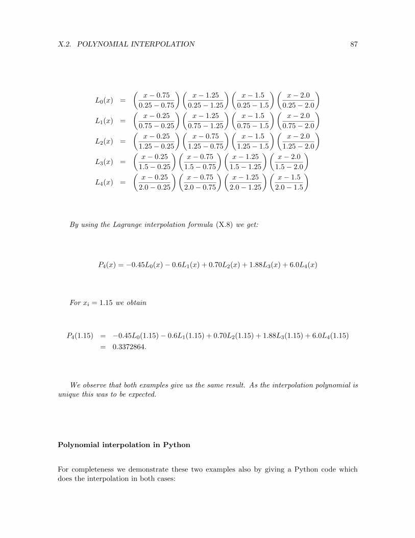
X.2. POLYNOMIAL INTERPOLATION 87
L0(x) =
(x− 0.75
0.25− 0.75
)(x− 1.25
0.25− 1.25
)(x− 1.5
0.25− 1.5
)(x− 2.0
0.25− 2.0
)L1(x) =
(x− 0.25
0.75− 0.25
)(x− 1.25
0.75− 1.25
)(x− 1.5
0.75− 1.5
)(x− 2.0
0.75− 2.0
)L2(x) =
(x− 0.25
1.25− 0.25
)(x− 0.75
1.25− 0.75
)(x− 1.5
1.25− 1.5
)(x− 2.0
1.25− 2.0
)L3(x) =
(x− 0.25
1.5− 0.25
)(x− 0.75
1.5− 0.75
)(x− 1.25
1.5− 1.25
)(x− 2.0
1.5− 2.0
)L4(x) =
(x− 0.25
2.0− 0.25
)(x− 0.75
2.0− 0.75
)(x− 1.25
2.0− 1.25
)(x− 1.5
2.0− 1.5
)
By using the Lagrange interpolation formula (X.8) we get:
P4(x) = −0.45L0(x)− 0.6L1(x) + 0.70L2(x) + 1.88L3(x) + 6.0L4(x)
For xi = 1.15 we obtain
P4(1.15) = −0.45L0(1.15)− 0.6L1(1.15) + 0.70L2(1.15) + 1.88L3(1.15) + 6.0L4(1.15)
= 0.3372864.
We observe that both examples give us the same result. As the interpolation polynomial isunique this was to be expected.
Polynomial interpolation in Python
For completeness we demonstrate these two examples also by giving a Python code whichdoes the interpolation in both cases:

88 CHAPTER 4. SUGGESTION OF PRESENTATION
from scipy import *
import scipy.linalg as sl
from matplotlib.pyplot import *
current=[0.25 , 0.75 , 1.25 , 1.5, 2.0] # current data
voltage=[-0.45 ,-0.6,0.70 ,1.88 ,6.0] # voltage drop data
plot(current ,voltage ,’*’)
x_plot=linspace(current[0], current[-1] ,100)
# ---------------------Monomial Basis ----------------------------
V=vander(current) # Vandermonde matrix
coef=sl.solve(V,voltage) # coefficients in monomial basis
y_plot=polyval(coef ,x_plot)
plot(x_plot ,y_plot)
p_i=polyval(coef ,1.15) # polynomial value at i=1.15
plot(1.15, p_i ,’o’)
plot([1.15,1.15],[-1,p_i],’-.’)# plot the line between point 1.15 and x axis
xlabel(’x’); ylabel(’y’)
print("""
Results
Vandermonde matrix {}
Coefficients {}
Polynomial Value {}""".format(V,coef ,p_i))
#--------------------Lagrange Basis ------------------------
def L(x,x_data ,i):
"""
Compute the i-th Lagrange basis function
x_data are the data points
"""
np1 = len(x_data)
return prod([(x-x_data[j])/(x_data[i]-x_data[j])
for j in range(np1) if j!=i])
def Lagrangeinterpolation(x,x_data ,y_data):
"""
Evaluate a polynomial at x
x_data , y_data interpoilation data
"""
np1 = len(x_data)
return sum([y_data[i]*L(x,x_data ,i) for i in range(np1)])
order = len(current) - 1 # order of polynomial
y_plot=[Lagrangeinterpolation(x,current , voltage) for x in x_plot]
plot(x_plot ,y_plot)
grid()

X.2. POLYNOMIAL INTERPOLATION 89
0.0 0.5 1.0 1.5 2.0x
1
0
1
2
3
4
5
6
7
y
Figure X.7: Plot of the 4th degree polynomial in different bases: monomial and Lagrangebasis give identical results.
Summary: how to construct interpolation polynomials
• The data points (x0, y0), . . . , (xn, yn), with xi distinct, uniquely define a polynomial Pnof degree n that interpolates the data, i.e., Pn(xi) = yi.
• The same polynomial can be expressed in different bases. It can be represented in themonomial basis
Pn(x) = anxn + an−1x
n−1 + · · ·+ a1x+ a0
or in the Lagrange basis
Pn(x) = y0
n∏j=1j 6=0
x− xjx0 − xj
+ y1
n∏j=0j 6=1
x− xjx1 − xj
+ · · ·+ yn
n∏j=1j 6=n
x− xjxn − xj
.
The construction of an interpolation polynomial depends on the chosen basis: the re-sulting coefficients differ for different bases but the polynomial itself is always the same.
X.2.3 Runge’s Phenomenon
This phenomenon was discovered by Carl David Tomle Runge in 1901. It is used to demon-strate a problem of higher order polynomial interpolation by considering the function
f(x) =1
1 + 25x2(X.9)

90 CHAPTER 4. SUGGESTION OF PRESENTATION
This function is commonly called Runge’s function. Data points are sampled on an equidis-tant grid of x-values in the interval [−1, 1]. The more points sampled, the higher is the orderof the interpolation polynomial. One observes large oscillations at both ends of the inter-val, causing a large interpolation error. This phenomenon demonstrates that high degreepolynomial interpolation can become unsuitable for polynomial interpolation on equidistantdata points. This phenomenon is demonstrated by the following Python code and the relatedfigures.
from scipy import *
from matplotlib.pyplot import *
def Runge(x):
"""
This is an implementation of Runge ’s function.
"""
return 1./(1. + 25.*x**2)
knots=int(input(’Number of knots\n’)) # asks for the number of knots
x_data = linspace (-1, 1, knots) # interval [-1,1] in 100 space
y_data = [Runge(x) for x in x_data]
"""
Polynomial interpolation
"""
coef = polyfit (x_data , y_data , knots-1) # polyfit function use to generate -
# coefficients of polynomial
x_plot = linspace (-1, 1, 100)
y_plot = polyval (coef , x_plot) # polyval function use to generate -
# a polynomial interpolation on x_plot
y_runge = [Runge(x) for x in x_plot]
plot(x_data , y_data , ’o’, label="data points")
plot(x_plot , y_plot , label="polynomial interpolation")
plot(x_plot , y_runge , ’--’, label="Runge ’s function")
grid()
legend(loc="best")

X.2. POLYNOMIAL INTERPOLATION 91
1.0 0.5 0.0 0.5 1.00.4
0.2
0.0
0.2
0.4
0.6
0.8
1.0
1.2
data pointspolynomial interpolationRunge's function
Figure X.8: Runge’s example: interpolation using 5 equally spaced data points and a 4th
degree polynomial.
1.0 0.5 0.0 0.5 1.01
0
1
2
3
4
5
6
7
8
data pointspolynomial interpolationRunge's function
Figure X.9: Runge’s example: interpolation using 15 equally spaced data points and a 14th
degree polynomial.

92 CHAPTER 4. SUGGESTION OF PRESENTATION
Note how the Python functions polyfit and polyval have been used. The functionpolyfit computes the polynomial coefficients and polyval evaluates the polynomial givenby these coefficients at particular points.
There is a danger of producing high oscillations when interpolating a large amount of data,because higher degree polynomials tend to have this unwanted behavior. That motivates tointroduce splines, and in particular cubic splines. These types of functions will be constructedby using only polynomials of low degree.
X.3 Piecewise polynomial Interpolation
To avoid the effect demonstrated by Runge’s function in the last section we will use piecewiseinterpolation polynomials to handle interpolation tasks with a large number of data points.
In this section you will guided gradually starting with the simplest approach – piece-wise linear polynomials – up to cubic splines, which are the most frequently used tool forinterpolation of a larger set of data points.
X.3.1 Piecewise linear Interpolation
Constructing a curve by connecting two subsequent data points by a straight line is calledlinear interpolation. Children use this technique already in kindergarten as a training game,cf. Figure X.10.
Figure X.10: Example for linear interpolation based on connecting numbered points to obtainthe shape of the G-clef.
I Mathematical Formulation of a piecewise linear function
Let us assume a set of n+ 1 data points,
(x0, y0), ..., (xi, yi), ...(xn, yn)

X.3. PIECEWISE POLYNOMIAL INTERPOLATION 93
with x0 < · · · < xi < xi+1 < · · · < xn. Then the linear function connecting (xi, yi) and(xi+1, yi+1) is
Si(x) = aix+ bi on [xi, xi+1) (X.10)
where ai, and bi are coefficients determined by the interpolation conditions Si(xi) = yi andSi(xi+1) = yi+1,
aixi + bi = yi (X.11)
aixi+1 + bi = yi+1 (X.12)
This gives
bi = yi − aixi (X.13)
Then, substituting (X.13) into (X.12) gives
aixi+1 + yi − aixi = yi+1 (X.14)
and finally
ai =yi+1 − yixi+1 − xi
bi =yixi+1 − yi+1xixi+1 − xi
.
The function S defined by these polynomials,
S(x) = Si(x) for x ∈ [xi, xi+1)
is called a linear piecewise polynomial.By construction these piecewise polynomials are continuous. Continuous linear piecewise
polynomials are called linear splines.Substituting the values of the coefficients ai, and bi into Eq. (X.10) gives
Si(x) = yixi+1 − xxi+1 − xi
+ yi+1x− xixi+1 − xi
(X.15)
This is the formula for each linear spline segment. Written in a general way, for the entireinterval,
S(x) = yixi+1 − xxi+1 − xi
+ yi+1x− xixi+1 − xi
for x ∈ [xi, xi+1). (X.16)
We see how easy the calculation of a linear interpolating spline is. The spline is fullydetermined by the data. No extra conditions are required to set up this function.
Example 3. Again, we consider the weather data reported from Lund city(Sweden) on April,4, 2017 given in Table X.2. The linear spline interpolating this data is displayed in Fig. X.11
Table X.2: Temperature data in Lund on April 4, 2017
Hour 0 1 2 3 4 5 6 7 8 9 10 11
Temperature◦C 5.7 5.1 4.5 3.9 3.8 3.8 3.9 3.5 4.2 6.4 8.2 9.6
Hour 12 13 14 15 16 17 18 19 20 21 22 23
Temperature◦C 10.4 10.8 11.5 11.9 11.8 11.8 11.5 10.4 8.6 7.3 6.5 5.9

94 CHAPTER 4. SUGGESTION OF PRESENTATION
0 3 6 9 12 15 18 21 24Hour
4
6
8
10
12
Tem
pera
ture
C
Data pointsInterpolation of 24 data
Figure X.11: Linear spline interpolating weather data given in Tab. X.2.
By construction, linear spline interpolation gives us a continuous function, but at theknots the first derivative is generally not continuous, as can be observed in this example. Formany applications this curve is not smooth enough. This motivates us to study quadraticspline interpolation and cubic spline interpolation to gain more smoothness.
X.3.2 Quadratic Spline Interpolation
A quadratic spline segment is given by the formula
Si(x) = ai(x− xi)2 + bi(x− xi) + ci on [xi, xi+1), (X.17)
which is written – as in the linear case – in a form centered around xi. We have three un-knowns per segment, namely ai, bi, ci. If there are n+1 data points, (x1, y1), . . . , (xn+1, yn+1),then the number of segments is n, so we have to find conditions to determine a total of 3nunknown coefficients.
There are n+1 interpolation conditions. Furthermore, asking for continuous and continu-ously differentiated segment connections we get 2n− 2 additional conditions. There is a totalof 3n − 1 conditions for 3n unknowns, which allows us one free “wish”. We can choose anextra condition in many different ways. Often, the slope at the left or at the right boundaryis prescribed. This gives the following relations:
• Interpolation: Si(xi) = yi, for i = 1, . . . , n, and interpolation at the endpointSn(xn+1) = yn+1.
• Continuity: Si(xi+1) = Si+1(xi+1) for i = 1, . . . , n− 1.
• Continuous derivative: S′i(xi+1) = S′i+1(xi+1) for i = 1, . . . , n− 1.

X.3. PIECEWISE POLYNOMIAL INTERPOLATION 95
Thus, to find the coefficients of a quadratic spline segment we make use of these conditions.From the interpolation condition and the form of the spline segment function we obtaindirectly ci = yi for i = 1, . . . , n. Then, we set zi = S′i(xi). As S′i(xi) = bi we obtain bi = zifor i = 1, . . . , n. So, the continuity conditions for the first derivative gives
ai =zi+1 − zi
2(xi+1 − xi), for i = 1, . . . , n− 1 (X.18)
while the coefficient an of the last segment is obtained from the end interpolation condition:
an =
yn+1−ynxn+1−xn − zn2(xn+1 − xn)
. (X.19)
To determine the remaining unknowns, zi, we make use of the continuity condition whichresults in
zi+1 + zi = 2yi+1 − yixi+1 − xi
for i = 1 . . . , n− 1. (X.20)
To simplify these expressions we introduce hi = xi+1−xi and write (X.20) in matrix-vectorform
h1 0h2 h2
. . .. . .
hj hj. . .
. . .
0 hn−1 hn−1
z2z3...
zj+1...zn
= 2
y2 − y1 − 12h1z1
y3 − y2...
yj+1 − yj...
yn − yn−1
(X.21)
You see that we left in the right-hand side of this equation the unknown z1. We choosethis as the additional degree of freedom, the “wish” we mentioned before. The formulationsimplifies if we set the slope at the left boundary to zero, z1 = w1 = 0. If we furthermoreassume equidistant data, i.e., h = h1 = · · · = hn we obtain from (X.22) the simplified form:
1 01 1
. . .. . .
1 1. . .
. . .
0 1 1
z2z3...
zj+1...zn
= 2
h
y2 − y1y3 − y2
...yj+1 − yj
...yn − yn−1
(X.22)
Note the special structure of the matrix. It has only entries on two diagonals – the maindiagonal and one subdiagonal. This type of matrix is called banded. Linear systems withbanded matrices can be cheaply solved by special algorithms. Another, perhaps even moreimportant observation is the way how we used the extra degree of freedom. We fixed it bya condition on the left boundary. Why at the left? We could as well have fixed it at theright boundary. The situation would have been even better if we would have a free wish for

96 CHAPTER 4. SUGGESTION OF PRESENTATION
both boundaries. This would not favor (or bind) a particular boundary. This unsymmetricalbehavior is typical for splines with an even degree, here degree two.
This approach, like the approach for linear splines and, later in this chapter, the approachfor cubic splines, uses the same points for nodes and knots. Recall that the nodes are theinterpolation points and the knots are the points where spline segments join. We refer to thisapproach as “nodes=knots”.
Example 4. Again, we consider the temperature data from Lund, cf. Tab. X.2 and interpolateit now with quadratic splines of the type ”nodes=knots”. The result is displayed in Fig. X.12.
0 3 6 9 12 15 18 21 24Hour
4
6
8
10
12
Tem
pera
ture
C
Data points
quadratic spline interpolation
Figure X.12: “Nodes=knots”-type quadratic spline interpolation of temperature data fromLund, Sweden. The boundary condition w1 = 0 at the left boundary is indicated.
There is a second approach to quadratic spline interpolation, which has one more degree offreedom. This extra degree of freedom is used as a second boundary condition in order to treatboth boundaries in a more balanced way. For this approach we allow the nodes and knots tobe different points and therefore refer to this approach by the acronym “knots6=nodes”. Theknots ki are chosen to be the midpoints of the node intervals. To develop this case we assumedata points (x1, y1), . . . , (xn+1, yn+1) and define n+ 1 knots ki by
k1 = x1, ki =xi−1 + xi
2, kn+1 = xn,
As before we express a spline segment as
Si(x) = ai(x− xi)2 + bi(x− xi) + ci on [ki, ki+1) (X.23)
but note now the different roles of xi and ki.The conditions for defining the unknown coefficients are now

X.3. PIECEWISE POLYNOMIAL INTERPOLATION 97
• Interpolation: Si(xi) = yi, for i = 1, . . . , n and interpolation at the end pointSn(xn+1) = yn+1.
• Continuity: Si(ki+1) = Si+1(ki+1), for i = 1, . . . , n− 1
• Continuity derivative: S′i(ki+1) = S
′i+1(ki+1) for i = 1, . . . , n− 1
Thus, the first interpolation property gives ci = yi. The continuity property results in
Si(ki+1) = Si+1(ki+1) : h2i ai − h2i ai+1 + 2hibi + 2hibi+1 = 2(yi+1 − yi) (X.24)
From continuity of the first derivative requirement we obtain
S′i(ki+1) = S
′i+1(ki+1) : hiai + hiai+1 + bi − bi+1 = 0 (X.25)
To simplify the expressions we set hi = xi+1 − xi and write a linear system of equationsfrom Eqs. (X.24) and (X.25) to solve for the unknown coefficients of the quadratic splinesegments. In addition, by finding the first derivative of quadratic spline segment we obtainSi(x) = 2ai(x−xi) + bi. Finally we use boundary conditions at each boundary by prescribingslopes S
′1(x1) = w1 S
′n(xn) = wn. This results in b1 = w1 and bn = wn. In total,
C1
H1
Hi
Hn−1Cn
a1b1a2b2...aibiai+1
bi+1...
an−1bn−1anbn
= 4
w1
y2 − y10
y3 − y20...
yi+1 − yi0...
yn − yn−10wn
(X.26)
with
Hj =
(h2j 2hj −h2j 2hjhj 1 hj −1
), C1 =
(0 1 0 0
), and Cn =
(0 0 0 1
)The matrix is banded matrix as the one in the previous case. Thus, the linear system is
not expansive to compute.
Example 5. Quadratic spline interpolation of the type “knots6=nodes” applied to the weatherdata from Tab. X.2 gives the curve displayed in Fig. X.13.

98 CHAPTER 4. SUGGESTION OF PRESENTATION
0 3 6 9 12 15 18 21 24Hour
4
6
8
10
12
Tem
pera
ture
C
nodes (data points)
knots
quadratic spline
Figure X.13: Quadratic spline interpolation of temperature data from Lund, by using theapproach “nodes 6=knots” and boundary values w1 = 0 and wn = 0. These are the slopesindicated at the left and right boundary of the figure.
X.3.3 Cubic Spline Interpolation
In previously presented types of splines interpolation, linear spline interpolation, and quadraticspline interpolation, we saw the advantages and disadvantages of those splines for interpolat-ing given data. Mainly, these lower order splines do not have continuous second derivatives.This motivates to study cubic splines as a tool of smooth interpolation of a big amount ofdata. To contrast it to polynomial interpolation of many data points, we consider againRunge’s function and the related Runge’s phenomenon which was used to demonstrate theproblems with high degree polynomial interpolation. We will see how cubic splines interpola-tion behave much better on that problem than polynomial interpolation or lower order splineinterpolation.
A cubic spline segment is given by the formula:
Si(x) = ai(x− xi)3 + bi(x− xi)2 + ci(x− xi) + di, on [xi, xi+1) (X.27)
We have four unknowns per segment, namely ai, bi, ci, di. If we have n + 1 data points,(x1, y1), . . . , (xn+1, yn+1), there are n segments. Therefore, we have to find conditions todetermined in total 4n unknowns coefficients.
X.3.3.1 What are the conditions to determine an interpolation cubic spline?
The interpolation and continuity conditions determine an interpolatory cubic spline

X.3. PIECEWISE POLYNOMIAL INTERPOLATION 99
• Interpolation: Si(xi) = yi, for i = 1, . . . , n and interpolation at the end pointSn(xn+1) = yn+1.
• Continuity: Si(xi+1) = Si+1(xi+1) for i = 1, . . . , n− 1.
• Continuous first derivative: S′i(xi+1) = S
′i+1(xi+1) for i = 1, . . . , n− 1.
• Continuous second derivative: S′′i (xi+1) = S
′′i+1(xi+1) for i = 1, . . . , n− 1.
As each of the n cubic spline segments has four unknown coefficients, our description of thefunction S involves 4n unknowns coefficients. The interpolation properties impose n+1 linearconstraints and the continuity properties impose 3(n−1) linear constraints on its coefficients.Therefore, there are a total of n+ 1 + 3(n−1) = 4n−2 linear constraints for the 4n unknowncoefficients. As the problem is not fully determined by these conditions there are infinitymany cubic splines passing through a given set of data points (x1, y1), ..., (xn, yn). In orderto uniquely define a cubic spline we have to arrive at a linear system, that has the samenumber of equations as unknowns. Therefor we need to add two more linear constraints (twofree wishes). There are various ways of specifying these two additional constraints leadingto different splines, e.g., natural cubic splines, curvature-adjusted cubic splines, and clampedcubic splines. These differ by the way how end conditions are selected. This selection isoften motivated by the actual case of application. The simplest way of adding two morelinear constraints is to put them as conditions at x1 and xn. That’s why we call them endconditions.
I Natural cubic splines The most commonly used end conditions are:
S′′1 (x1) = 0 , S
′′n(xn) = 0.
A spline satisfying these conditions is called a “natural” spline because - as we will see laterit plays an important role in the elasticity of beams.
Example 6 (Natural cubic splines). Consider again the the problem to interpolate Runge’sfunction, see Sec. X.2.3:
f(x) =1
1 + 25x2(X.28)

100 CHAPTER 4. SUGGESTION OF PRESENTATION
1.0 0.5 0.0 0.5 1.0x
0.0
0.2
0.4
0.6
0.8
1.0
y
Figure X.14: Natural cubic splines interpolation of Runge’s function.
Figure X.14 shows how nicely a natural cubic spline describes Runge’s function withoutoscillation at the boundary regions of the interval. By comparing with the polynomial coun-terpart in Sec. X.2.3 we see why cubic spline interpolation is to be prefered.
I Curvature-adjusted cubic spline The alternative approach to a natural cubic splinerequires setting:
S′′1 (x1) = a , S
′′n(xn) = b
As we observe at the second derivative we have arbitrary choice a, and b these instead ofzero in natural cubic spline interpolation.
I Clamped cubic splines A clamped cubic splines is defined by its first derivative at thefirst and last nodes:
S′1(x1) = a , S
′n(xn) = b
It is called a “clamped” spline because “it is what occurs when you clamp the end of adrafting spline so that is has a desired slope” Chapra [2011]. For example, when we drive ona bridge the ends of bridge have been such, that their slopes fit to the slope of the connectingstreets, cf., Figure X.15. Ideally, a clamped cubic spline interpolating certain given supportingpoints is the way to describe such a bridge. Thus, the slope at the beginning and end of thespline are under users control.

X.3. PIECEWISE POLYNOMIAL INTERPOLATION 101
Figure X.15: Dalal bridge in Zakho, Iraq, which dates to the Roman era. The picture behindthe clamped curve is taken from Ancient Art [2017].
Additionally, there are several more cases of end conditions cubic splines for exampleparabolically terminated cubic splines, and not-a-knot cubic spline. Here the end conditionsare not set by physical or technical consideration. Often, when the interpolation result is notstatisfactory a change of the type of end conditions is made. For example in Runge’s examplewe observe that natural cubic spline interpolation results in a good description of Runge’sfunction. If we use different types of end conditions maybe we do not get qualitatively thesame result as if natural cubic spline were chosen. The following Figure X.16 shows Runge’sfunction interpolated with a clamped spline with the choice S
′1 = 1 and S
′n−1 = −1.
X.3.3.2 Construction of an interpolatory cubic spline.
Here we will show how to compute the coefficients of a spline segment:
Si(x) = ai(x− xi)3 + bi(x− xi)2 + ci(x− xi) + di on [xi, xi+1) (X.29)
The continuity and interpolation conditions are
condition number
(1) Si(xi) = yi, and Sn(xn+1) = yn+1 i = 1, . . . , n n+ 1
(2) Si(xi+1) = Si+1(xi+1), i = 1, . . . , n− 1 n− 1
(3) S′i(xi+1) = S
′i+1(xi+1), i = 1, . . . , n− 1 n− 1
(4) S′′i (xi+1) = S
′′i+1(xi+1), i = 1, . . . , n− 1 n− 1
(5) S′′1 (x1) = 0, 1
(6) S′′n(xn+1) = 0, 1
total=4n (X.30)
We have two boundary end conditions (5), and (6) in Eq. (X.30). In total we have now afully determined system with 4n conditions for the 4n unknowns.From them we can computethe coefficients of the cubic spline segment (X.29):

102 CHAPTER 4. SUGGESTION OF PRESENTATION
1.0 0.5 0.0 0.5 1.0x
0.0
0.2
0.4
0.6
0.8
1.0
y
Figure X.16: Runge’s function with 10 points and clamped end conditions stating that firstderivatives at the left and right boundaries being +1 and -1, respectively.
1. The first property, Si(xi) = yi, which is an interpolation condition, gives:
di = yi (X.31)
2. The second property, Si(xi+1) = Si+1(xi+1), states that curve a cubic spline is continu-ous at at the nodes. From this and by setting hi = xi+1 − xi we obtain:
aih3i + bih
2i + cihi + di = di+1 (X.32)
Additionally, the first derivatives at the interior nodes of cubic spline segment must byequal.
S′i(xi+1) = 3aih2i + 2bihi + ci = ci+1 = S′i+1(xi+1) (X.33)
Correspondingly, for the second derivatives we get
S′′i (xi+1) = 6aihi + 2bi = 2bi+1 = S′′i+1(xi+1). (X.34)
3. Now, we will introduce new variables for second derivatives at xi:

X.3. PIECEWISE POLYNOMIAL INTERPOLATION 103
ψi := S′′i (xi) = 2bi (X.35)
and express bi by
bi =ψi2
(X.36)
4. From Eq. (X.34) we conclude
ai =bi+1 − bi
3hi(X.37)
By substituting (X.36) into (X.37) we get:
ai =ψi+1 − ψi
6hi(X.38)
and by substituting Eq.(X.36) and Eq.(X.38) in Eq.(X.32) we get:
ci =yi+1 − yi
hi− hi
(2ψi + ψi+1)
6(X.39)
As we observe all unknowns coefficients can be expressed in terms of the ψ.
5. From Eq. (X.33) we obtain now by inserting the expressions for ai, bi and ci:
3(ψi−ψi−1
6hi−1
)h2i−1 + 2ψi−1
2 hi−1 +(yi−yi−1
hi−1
)− hi−1 (2ψi−1+ψi)
6 =(yi+1−yi
hi− hi (2ψi+ψi+1)
6
)and finally,
hi−1ψi−1 + 2(hi−1 + hi)ψi + hiψi+1 = 6
(yi+1 − yi
hi− yi − yi−1
hi−1
)(X.40)
6. By then using conditions (5) and (6) Eq. (X.30) obtain have a linear system to computethe vector ψ from which we determine all coefficients of the cubic spline segment formula.
Consequently, we can write the linear system with the two boundary conditions as free“wishes” which can be expressed as ψ1 = w1, and ψn+1 = w2.
In the case of natural splines these ”wishes” are w1 = 0 and wn+1 = 0. For naturalcubic splines, S′′n(xn+1) = 0 implies that ψn+1 = 0.
The following system what we need to solve is:{hi−1ψi−1 + 2(hi−1 + hi)ψi + hiψi+1 = 6
(yi+1−yi
hi− yi−yi−1
hi−1
)ψ1 = ψn+1 = 0
or more compactly,
Hψ = y.

104 CHAPTER 4. SUGGESTION OF PRESENTATION
1 0h1 2(h1 + h2) h2
h2 2(h2 + h3) h3h3 2(h3 + h4) h4
. . .
hn−2 2(hn−2 + hn−1) hn−10 1
ψ1
ψ2
ψ3
ψ4......ψnψn+1
=
= 6
w1y3−y2h2− y2−y1
h1y4−y3h3− y3−y2
h2......
yn+1−ynhn
− yn−yn−1
hn−1
wn+1
(X.41)
The system matrix is strictly diagonally dominant as its diagonal elements are larger thanthe sum of the off-diagonal elements. This property guarantees that a matrix is invertible.Consequently the system has a unique solution ψ.
Furthermore, the matrix is banded – more precisely it is tridiagonal. Solving linear systemswith tridiagonal matrices is fast.
Finaly we note, that H can easily be constructed in Python from an array containing thestep sizes hi:
h=diff(array(x))
H=diag([1]+list(2*(h[:-1]+h[1:]))+[1])+diag(list(h[:-1])+[0],-1)+\
diag([0]+list(h[1:]),+1)
As pointed out before the definition of cubic spline leaves two degree of freedom “wish”. Inour case we choose natural cubic spline end conditions, but we have different kind of endconditions can by satisfies our linear system as well, for example:
• Clamped end conditions:
These end conditions prescribe the slopes at the boundary points. So, S′(x0) andS′(xn) are given. Thus, the conditions of ψ0 and ψn can be derived and a linear systemcorresponding to Eq. (X.41) can be set up.
• Not-a-knot end conditions:
This end conditions enforces continuity of the third derivative at the second and thenext to last knots:
S′′′1 (x2) = S′′′2 (x2), S′′′n−1(xn) = S′′′n (xn) (X.42)

X.3. PIECEWISE POLYNOMIAL INTERPOLATION 105
Common third derivatives make the first and second spline segment a common thirddegree polynomial, which is as if the second knot would be replaced and just a nodefor the interpolation would be left over at that place. That’s why this end-condition iscalled a “not-a-knot” condition.
I We sum up all steps to find the coefficients of a cubic interpolatory spline:
1. Condition, interpolation: Si(xi) = yi we get: di = yi
2. Condition, continuity of the second derivative S′′i (xi+1) = S
′′i+1(xi+1) we get: bi =
ψi2
,
and ai =ψi+1 − ψi
6hi
3. Condition, continuity of the function Si(xi+1) = Si+1(xi+1) we get:
ci =yi+1 − yi
hi− hi
(2ψi + ψi+1)
6
4. Condition, continuity of the first derivative S′i(xi+1) = S
′i+1(xi+1) we get:
hi−1ψi−1 + 2(hi−1 + hi)ψi + hiψi+1 = 6
(yi+1 − yi
hi− yi − yi−1
hi−1
).
Additionally two boundary conditions are used to fix the remaining two degrees offreedom.
Example 7. We use the same data points as in Example 1 which describes voltage drops Viacross a resistor for a number of different current values xi. From this data we now constructa cubic spline and compute the voltage drop at x = 1.15 A.
In the first step we use Eq. (X.41) to determine the coefficients ψ. So, we have to solvelinear system of equations :
1 0 0 0 00.5 2. 0.5 0 00 0.5 1.5 0.25 00 0 0.25 1.5 0.50 0 0 0 1
ψ0
ψ1
ψ2
ψ3
ψ4
=
0
17.412.7221.12
0
This equation can be solved by using Python or Matlab. The result is
ψ =(0. 7.790625 3.6375 13.47375 0
)Now we can find the coefficients of each cubic spline segment S1, S2, S3 to be
i ai bi ci di1 2.596875 0 -0.94921875 -0.452 -1.384375 3.8953125 0.9984375 -0.63 6.5575 1.81875 3.85546875 0.704 -4.49125 6.736875 5.994375 1.88

106 CHAPTER 4. SUGGESTION OF PRESENTATION
Then we will have:
S1(x) = 2.596875(x− 0.25)3 − 0.94921875(x− 0.25)− 0.45
S2(x) = −1.384375(x− 0.75)3 + 3.8953125(x− 0.75)2 + 0.9984375(x− 0.75)− 0.6
S3(x) = 6.5575(x− 1.25)3 + 1.81875(x− 1.25)2 + 3.85546875(x− 1.25) + 0.70
S4(x) = −4.49125.(x− 1.25)3 + 6.736875(x− 1.25)2 + 5.994375(x− 1.25) + 1.88
To evaluate the spline, at for example x = 1.15, one first has to find the knot intervalto which x belongs, here the second interval, and then one evaluates the corresponding splinesegment:
S2(1.15) = −1.384375(1.15− 0.75)3 + 3.8953125(1.15− 0.75)2 + 0.9984375(1.15− 0.75)− 0.6
= 0.33402499
Example 8. By using the same data temperature data reported from Lund city (Sweden) onApril, 4, 2017 X.2. The cubic spline interpolation this data display in Figure
0 3 6 9 12 15 18 21 24Hour
3
4
5
6
7
8
9
10
11
12
Tem
pera
ture
◦ C
data pointscubic spline interpolation
Figure X.17: Cubic spline interpolation of temperature Lund city in Sweden.
The plot of the cubic spline interpolating the temperature Lund city shows that a cubicspline results in a smoother curve than the one obtained by quadratic spline interpolation andlinear spline interpolation. Also, cubic spline interpolation is the better choice for interpolationthen interpolation by higher degree polynomials.

X.3. PIECEWISE POLYNOMIAL INTERPOLATION 107
X.3.3.3 Why cubic spline interpolation?
The term smoothness normally refers to continuity of the function and its derivatives. In thecontext of splines we also often speak about smoothness, when we want to emphasize thatthe curve has no ”unnecessary oscillations.” In this section we demonstrate why cubic splineshave optimal smoothness also in this sense.
We consider as a measure of smoothness the integral∫ ba [f
′′(x)]2dx which measures accu-
mulated curvature.The following theorem states a minimality property of cubic splines with respect to this
measure:
Theorem (Optimality of Natural Splines).Let f
′′be continuous in [a, b] and let a = x0 < x1 < . . . < xn = b. If S is the natural cubic
spline interpolating f at the knots xi for 0 ≤ i ≤ n then:∫ b
a[S′′(x)]2dx ≤
∫ b
a[f′′(x)]2dx
Proof :Let consider the difference between S and f
g(x) = f(x)− S(x) (X.43)
Consequently,(f′′)2 = (S
′′)2 + (g
′′)2 + 2S
′′g′′
(X.44)
and ∫ b
a(f′′)2dx =
∫ b
a(S′′)dx+
∫ b
a(g′′)2 +
∫ b
a2S′′g′′dx (X.45)
If we can show ∫ b
aS′′g′′dx = 0 (X.46)
than we conclude ∫ b
a(f′′)2dx ≥
∫ b
a(S′′)2dx (X.47)
which would complete the proof.Let us proof no why (X.46) holds. Firstly, we integrate by parts,∫
abS′′g′′dx = S
′′g′∣∣∣ba−∫abS′′′g′dx
Since S′′(a) = S
′′(b) = 0 by natural cubic spline conditions, the first term zero. Addition-
ally, in the second term, since S′′′
segment is constant we set
ci = S′′′(x), forx ∈ [ti, ti+1].
Then

108 CHAPTER 4. SUGGESTION OF PRESENTATION
∫ b
aS′′g′dx =
n−1∑i=0
ci
∫ xi+1
xi
g′(x)dx
andn−1∑i=0
ci[g(xi+1 − g(xi))] = 0.
X.3.3.4 Discussion
We have seen that linear spline interpolation is easy to calculate and it is continuous, but isnot smooth. We have looked at two types of quadratic spline interpolation. In the first case,“nodes=knots,” we obtain one boundary condition, and in the second case, “nodes 6=knots,”we get two boundary conditions. This second case seemed to yield a better result. Thefact that we have two boundary conditions means that we have more freedom too choose, andthus more control of both sides of the spline curve. Cubic spline interpolation shows smootherresults than the other kinds of spline interpolation because in cubic spline interpolation weget two boundary conditions and because of the higher degree we get a smoother curve.
We notice that if we consider splines with “nodes=knots,” those of even degree will havean odd number of boundary conditions, and those of odd degree will have an even numberof boundary conditions, which translates to having equal control over each end of the curve.The proof of this statement is as follows:
Consider a polynomial of degree k, and n + 1 interpolation points. Then there will ben spline segments. To find the coefficients of the spline we must have an equal number ofconditions and unknowns. We have (k + 1) coefficients for each polynomial segment, so wewill have n(k+1) coefficients for the entire spline. From the properties of cubic splines we getn+ 1 interpolation conditions and k(n− 1) continuity conditions. Thus, the total number ofconditions given by the properties of the spline is (nk+ 1) + k(n− 1). Consequently, we needadditional n(k+ 1)− k(n− 1)− (n+ 1) = k− 1 end conditions. Thus, when the degree of thepolynomial k is even we will have an odd number of boundary conditions and viceversa.
X.3.4 A historical fact of cubic splines interpolation.
The first picture, Figure X.18, was shown to students of the course Seminar in NumericalAnalysis in 2015 at Lund University during a lecture on spline interpolation. The pictureshows the construction of a spline by using “duck” lead weights. It was our personal experiencethat this picture increased our enthusiasm discover more about the history of cubic splinesby researching how the “ducks” were used to construct a cubic spline.
Figure X.19 shows a course in airplane design in 1941. A cubic spline is constructed inorder to shape a turbine blade. The “ducks” are used to arrive to the smoothest possibleshape. The lead weights are “called ducks because of their duck-like shape” [spline, 2017].It is commonly accepted that the first mathematical reference to splines is 1946. The word“spline” was used in connection with smooth, piecewise polynomial approximation.

X.3. PIECEWISE POLYNOMIAL INTERPOLATION 109
Figure X.18: The drafting technique of a spline by using duck lead weights. In 1997 at RollsRoyce in Karlshamn, Sweden.

110 CHAPTER 4. SUGGESTION OF PRESENTATION
Duck
Spline
Turbine
blade
shape
Figure X.19: Course in Airplane Lofting, Burgard High School, Buffalo, NY, USA, January1, 1941 (Digital Remediation [2017])

Chapter 5
Conclusion and Future Work
The aim of this thesis is to describe and study different methods of teaching in several numer-ical analysis books to arrive to a good strategy for the teaching of cubic spline interpolation.As future work we would like to further the development of the didactic methods for theteaching of other topics in a numerical analysis course. When we add exercises in any topicwe must take into account the critical points as we discussed in the introduction of Chapter 4.The list of exercises should be such that after solving them a student can feel certain that hehas understood well the topic. This will give students a motivation to develop their scientificskills in the subject. It is also important to develop the practical aspect of teaching. Evenwhen using the same textbook, different teachers will approach the topic differently whenthey are in front of a class. What a teacher does and says in front of the audience will clarifythe contents of the textbook. A teacher in front of the blackboard will affect students morethan the actual textbook contents. Consequently, by using the comparison criteria in 2.1 wecan develop various topics in numerical analysis in order to find a good teaching strategy.
111

112 CHAPTER 5. CONCLUSION AND FUTURE WORK

Bibliography
A project by the government of India (2017). https://onlinecourses.nptel.ac.in/noc17 ge02/preview.[Online; accessed 11 March 2017].
Ancient Art (2017). http://ancientart.tumblr.com/page/66. [Online; accessed 29 April 2017].
Chapra, S. C. (2011). Applied Numerical Methods with MATLAB for Engineers and Scientists.McGraw-Hill Education / Asia, 3nd edition.
Digital Remediation (2017). http://cornelljournalofarchitecture.cornell.edu/read.html?id=74.[Online; accessed 05 March 2017].
Duke University (2015). https://services.math.duke.edu/∼djl/teaching/math361spring2015/syllabus.pdf.[Online; accessed 11 March 2017].
Fausett, L. V. (2008). Applied Numerical Analysis Using MATLAB. Pearson Prentice Hall,NJ, 3nd edition.
Hacettepe Universitesi (2017). http://yunus.hacettepe.edu.tr/∼edacelik/231-web/info.htm.[Online; accessed 11 March 2017].
Harvard University (2012). http://isites.harvard.edu/icb/icb.do?keyword=k89160&pageid=icb.page522356.[Online; accessed 11 March 2017].
Introduction to Computer Graphics (2017). http://www.kharwal.com/introduction-to-computer-graphics/. [Online; accessed 23 April 2017].
Kincaid, D. and Cheney, W. (2002). Numerical Analysis. American Mathematical Society,Providence, RI, 3nd edition.
Maghdid, D. (2016). Comparative study of teaching computational mathematics in two differ-ent learning environments. PhD thesis.
McMaster University (2014). http://www.ece.mcmaster.ca/∼xwu/outline3SK3.htm. [Online;accessed 11 March 2017].
Sauer, T. (2012). Numerical Analysis. Pearson Education, Inc, 2nd edition.
spline, F. (2017). http://en.wikipedia.org/wiki/Flat spline. [Online; accessed 05 March 2017].
University, L. (2017). http://www.ctr.maths.lu.se/na/courses/FMN050/. [Online; accessed12 March 2017].
113

114 BIBLIOGRAPHY
University of Florida (2009). http://www2.mae.ufl.edu/haftka/numerical/. [Online; accessed11 March 2017].
Washington State University (2017). http://www.math.wsu.edu/faculty/genz/448/info.html.[Online; accessed 11 March 2017].

Appendix A
Example (Table lookup):
What is table lookup? And how can observe type of work called table lookup? What followsis a brief summary of table lookup using data from exponential functions:
�−� ��
�
�−�
��
�
0.0821 12.182 2.5 1.000 1.000 0.00
0.0743 13.464 2.6 0.9512 1.0513 0.05
0.0672 14.880 2.7 0.9048 1.1052 0.10
0.0608 16.445 2.8 0.8607 1.1618 0.15
0.0550 18.174 2.9 0.8187 1.2214 0.20
Figure A.1: Table exponential functions
In order to calculate the function ex when x = 2.4 is not in the previous table.
�
�
12.182 2.5
13.464 2.6
� � = 2.4 � =?
By using linear spline formula. The following are steps of solving:
S(x) = ax+ b (A.1)
115

116 APPENDIX A. EXAMPLE (TABLE LOOKUP):
S(2.5) = a(2.5) + b⇒ 12.182 = a(2.5) + b (A.2)
S(2.6) = a(2.6) + b⇒ 13.464 = a(2.6) + b (A.3)
By Subtracting the equations (2) from (3) will get:a = 12.82 and b = −19.868.
To find the function ex when x = 2.4:
S(2.4) = (12.82)(2.4)− 19.868 = 10.9 (A.4)
This work is called table lookup (what we are doing by using table whether the work byusing computer or hands called table look up)


![[LU, BILL CHANG] Executive MA Thesis 2015](https://static.fdocuments.in/doc/165x107/589b53ca1a28ab4a398b6f99/lu-bill-chang-executive-ma-thesis-2015.jpg)