School of Innovation, Design and Engineering

MASTER THESIS IN SOFTWARE ENGINEERING

30 CREDITS, ADVANCE LEVEL 120

Extending ABB’s WirelessHART Tool

Author(s): Andras Zakupszki and Nuttapon Pichetpongsa Email: azi10001@student.mdh.se and npa10001@student.mdh.se

Carried out at: ABB AB Coperate Research

Advisor at Malardalen University: Frank Lüders Advisor at ABB: Tiberiu Seceleanu

Examiner: Ivica Crnkovic Date: 23 August 2012

ii

Abstract

Within this decade, wireless technology has been used in process control in various

industries. WirelessHART is one of the standards, used for creating communication

networks for such purpose. Since the technology is relatively new, there are many

known and unknown risks in deploying it in real life applications.

ABB’s WirelessHART Tool is used for generating simulation scenarios that can be used

for evaluating the performance of WirelessHART networks under different conditions.

This paper describes in detail, how ABB’s WirelessHART Tool was extended by adding

various new functionalities. The topics cover what obstacles we have faced, which

solutions were used and why, how our solutions were evaluated and the outcomes.

Furthermore, the paper documents the application structure of WirelessHART Tool.

Keywords: WirelessHART, TrueTime, Simulink, MATLAB, Software, Simulator,

Networked Control Systems

iii

Acknowledgement

This thesis work would not have been possible without the support of many people.

We would like to express our gratitude to our academic advisor Frank Lüders, who was

greatly helpful and offered invaluable guidance.

We are truly indebted to our supervisor at ABB Tiberiu Seceleanu who was always

willing to help and support us.

We would also like to thank to our Thesis Examiner Professor Ivica Crnkovic.

We would like to show our gratitude to the staff at ABB who gave us their invaluable

opinions and guidance during discussions.

Finally, we would like to thank our beloved family because without their support and

encouragement the thesis would not have been completed.

iv

Acronyms

IEEE Institute of Electrical and Electronic Engineers

GUI WirelessHART tool Graphical User Interface

TDMA Time Division Multiple Access

CSMA/CA Carrier Sense Multiple Access with Collision Detection

MAC Medium Access Control

WHART WirelessHART

v

Table of Contents

1. Introduction ...................................................................................................................... 1 1.1 Problem Formulation ..................................................................................................................................................... 2 1.2 Report Outline ................................................................................................................................................................... 2

2. Background ....................................................................................................................... 4 2.1 Process Control in Industrial Production ............................................................................................................... 4

2.1.1 Closed loop control............................................................................................................................................................. 4 2.1.3 Proportional, Integral and Derivative Controller ............................................................................................... 6

2.2 Network Technologies ................................................................................................................................................... 7 2.2.1 The Open System Interconnection Model ................................................................................................................ 7 2.2.2 Wired Network Standards........................................................................................................................................... 10 2.2.3 Wireless Network Standards ...................................................................................................................................... 12

2.3 WirelessHART Technology ........................................................................................................................................ 17 2.3.1 Basic Components of WirelessHART ....................................................................................................................... 18 2.3.2 Medium Access Control ................................................................................................................................................. 20

2.4 Development Tools and Simulation Environment ........................................................................................... 27 2.4.1 MATLAB ............................................................................................................................................................................... 27 2.4.2 Simulink ............................................................................................................................................................................... 28 2.4.3 TrueTime ............................................................................................................................................................................. 29

3. ABB’s WirelessHART Tool ................................................................................................. 35 3.1 TrueTime Upgrades ...................................................................................................................................................... 35

3.1.1 TrueTime Network Block ............................................................................................................................................. 36 3.1.2 TrueTime Kernel Block ................................................................................................................................................. 37

3.2 Application Structure ................................................................................................................................................... 40 3.3 User Interface & Functionality .................................................................................................................................. 42

3.3.1 Create Model ...................................................................................................................................................................... 43 3.3.2 Network Property ............................................................................................................................................................ 44 3.3.3 Sensor Property ................................................................................................................................................................ 45 3.3.4 Actuator Property ........................................................................................................................................................... 46 3.3.5 Intermediate Node .......................................................................................................................................................... 46 3.3.6 Control Loop Properties ............................................................................................................................................... 46 3.3.7 Transmission Delay ........................................................................................................................................................ 47 3.3.8 Actions .................................................................................................................................................................................. 47 3.3.9 Schedule Table .................................................................................................................................................................. 48 3.3.10 Menu ................................................................................................................................................................................... 48

3.4 Simulation Model ........................................................................................................................................................... 49 3.5 Code Readability ............................................................................................................................................................. 54

4. Extensions to WirelessHART Tool ..................................................................................... 55 4.1 Requirements .................................................................................................................................................................. 55

4.1.1 Wired actuator ................................................................................................................................................................. 55 4.1.2 Multiple Channels ............................................................................................................................................................ 55 4.1.3 Toggle switch for sensor, actuator, intermediate panel ............................................................................... 55 4.1.4 Using the same color pattern for each control loop ........................................................................................ 56

vi

4.1.5 Remove node on scheduling table by using Delete Key .................................................................................. 56 4.1.6 Improving the correctness of Controller ............................................................................................................... 56

4.2 Limitations ........................................................................................................................................................................ 57 4.2.1 Internal Limitations ....................................................................................................................................................... 57 4.2.2 External Limitations ...................................................................................................................................................... 57

5. Solution ........................................................................................................................... 58 5.1 Application Structure ................................................................................................................................................... 58 5.2 User Interface Design ................................................................................................................................................... 58

5.2.1 Changes in Create Model .............................................................................................................................................. 59 5.2.2 Changes in Sensor/Actuator/Intermediate Property ..................................................................................... 59 5.2.3 Changes in Control Loop Property........................................................................................................................... 61 5.2.4 New Gateway Panel ........................................................................................................................................................ 62 5.2.5 Change in Schedule Table ............................................................................................................................................ 62

5.3 Simulation Model ........................................................................................................................................................... 64

6. Evaluation and Results ..................................................................................................... 71 6.1 Testing the Application ................................................................................................................................................ 71

6.1.1 The Reference Model ...................................................................................................................................................... 71 6.1.2 Test 1: The performance of the Old WirelessHART Tool and New WirelessHART Tool ................. 72 6.1.3 Test 2: The performance of Wireless Actuator and Wired Actuator ....................................................... 76 6.1.4 Test 3: The performance of Multi Channel and Single Channel ................................................................. 80

7. Discussion of Results ........................................................................................................ 84

8. Conclusion and Future work............................................................................................. 85

References .......................................................................................................................... 87

1

1. Introduction

Wireless technology is traditionally used in the communication and

telecommunication domain however nowadays it plays an important role in many other

disciplines as well. In the last few years, it has emerged in industrial process control to

provide an alternative to the already existing wired technology. The advantages are

reduced power consumption and weight of the machinery.

ABB is a one of the world’s leading engineering corporations mostly operating in

the areas of power and automation. ABB was created in 1988 by merging the Swedish

company ASEA (created in 1883) and the Swiss company Brown, Boveri & Cie (created

in 1891). In order to supply state of art technology to customers ABB Corporate

Research continuously performs research on a number of areas in order to ensure they

have the edge in environmental friendliness, sustainability, prices, and quality. One of

these research areas is automation networks more precisely wireless automation

networks.

WirelessHART (Wireless Highway Addressable Remote Transducer) is one of

the standards that are used for building communication networks for process control. It

is cost effective and ensures quick and easy installation. Nevertheless, when using

WirelessHART for process control, the critical point of the process needs to be

anticipated and evaluated from the point of efficiency. The behaviors of the process also

need to be predicted in case of packet loss, noise and other disturbances.

WirelessHART Tool is an application created by ABB to automate generating

WirelessHART network simulations. WirelessHART Tool was implemented in MATLAB

for increasing the speed of creating simulations for WirelessHART networks. It uses

Simulink along with a modified TrueTime library as simulation environment, which

enables simulation of packet loss and other network related problems.

2

1.1 Problem Formulation

The problem in the focus of this thesis is how to improve and extend WirelessHART

Tool without affecting already existing features.

In order to identify improvements that need to be performed, first the design of the

existing WirelessHART Tool has to be discovered and documented.

The contribution of this Thesis is to add two major extensions to WirelessHART Tool.

The first extension is to allow users to build simulations where both a wired and a

wireless network coexist.

The second extension is to allow the users to generate networks that use multiple

channels in their frequency range to transmit data.

Since before this thesis the application structure was not documented another

contribution is that the application structure was exposed and documented.

1.2 Report Outline

Chapter 2 contains information that is crucial for understanding the following chapters.

The topics cover process control, wired and wireless network technologies and

specifically focusing on WirelessHART. Other topics such as description of the used

tools, libraries, simulation environment are also included.

Chapter 3 starts with brief introduction of ABB’s WirelessHART Tool and the modified

TrueTime library developed by ABB is explained here.

Later, the reader can see a detailed specification and evaluation of ABB’s

WirelessHART Tool from a software engineering point of view. This includes structure,

coding style, functionality etc.

Chapter 4 includes the requirements collected from ABB in order to improve and extend

the tool. The scope and limitations of the work is covered here as well.

3

Chapter 5 contains the solutions for each requirement and the reasons for each of those

solutions.

Chapters 6 and 7 describe how the solutions were evaluated, what were the results of

those evaluations as well as the explanation of the results.

Chapter 8 concludes the paper and gives suggestions for further improvements for

ABB’s WirelessHART Tool and other related appliances.

4

2. Background

In this section, we describe briefly the fundamental information which was found during

research. There are three main areas that the reader should familiarize with before start

reading the next chapter. These three main areas are: Networking Technology,

Industrial Process Control and Software Development.

Section 2.1 provides a short explanation about process control used in industrial

production, focusing on closed loop control systems and a general description of the

PID controller.

Section 2.2 talks about the network technologies that were met during development for

example Ethernet and a few wireless standards. This subsection also includes a table

comparison about each kind of networks.

Section 2.3 focuses on describing the WirelessHART Standard.

Section 2.4 gives a brief introduction on the development tools that were used during

the implementation phase.

2.1 Process Control in Industrial Production

Process controllers are used in a large variety of areas such as oil refining, chemicals

and power plants. In industrial production, process controllers are used to manage

process output and keep it within the desired range. There are different controllers for

different kinds of processes.

2.1.1 Closed loop control

There are two major types of process control systems: open loop control systems and

closed loop control systems [3]. In this thesis, only the closed loop control systems are

observed.

5

A set of common terms used in the automated process control area need to be defined

for better understanding. There are some important variables that need to be named

and defined in the area of process control systems [1].

The controlled variable is the variable, which the process deals with. Sometimes the

term “process variable” also refers to the controlled variable.

Setpoint is a desired value of controlled variable. The action of the controller is based

on the error between the controlled variable and the setpoint. If the error is not 0, the

controller will try to drive the value of the controlled variable towards the setpoint.

Manipulated variable is the input to the actuator. The actuator uses it to affect the

process and keep the controlled variable on the desired setpoint.

Error is the difference between the feedback and the setpoint. The error can be either

positive or negative. The purpose of any controllers is to minimize an error.

The feedback is the input to the sensor (output from the process) that needs to be

maintained or controlled at the desired value (setpoint). Feedback control reacts to

system and works to minimize the error.

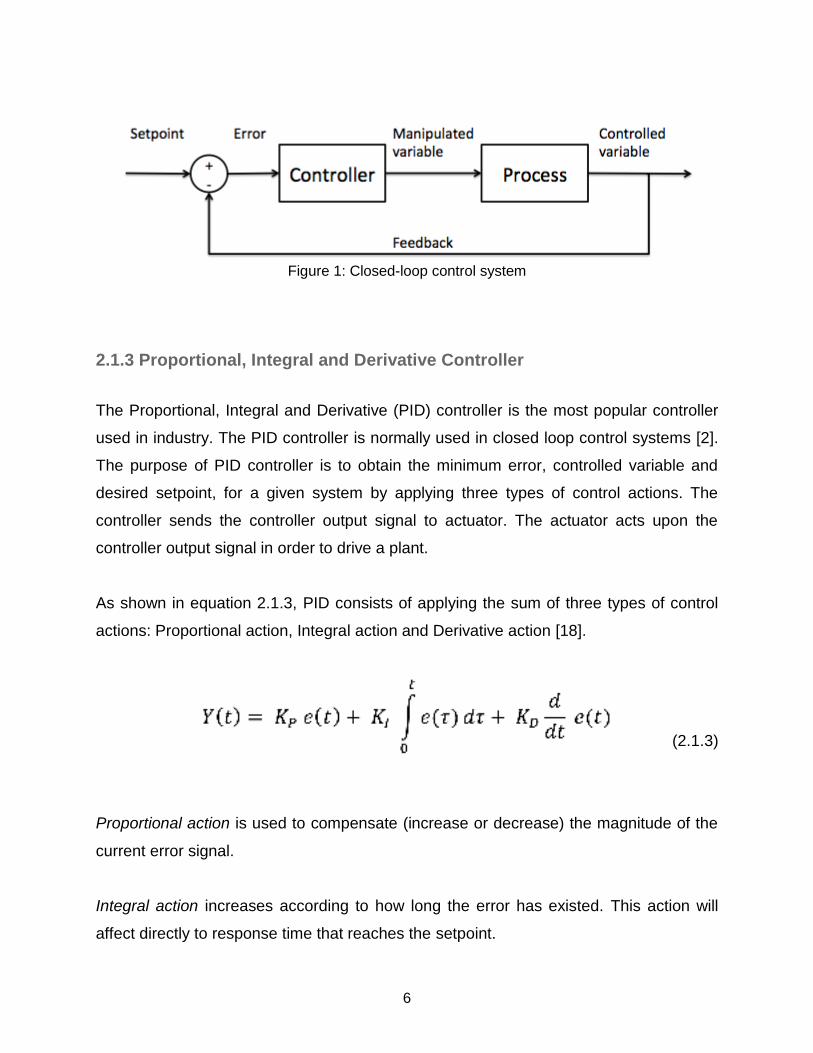
Referring to Figure 1, closed loop control system uses error between the feedback

from the process compare to the desired setpoint to make a decision of changing the

control signal that drives the system. The feedback is current output from the process

that is observed. In the control system term, the error value can be positive or negative.

The controller persists to maintain the error to reach the desired state. The error will be

adjusted accordingly to the desired setpoint by sending manipulated variable to the

process. Since closed loop control system can adjust itself, from time to time, it is called

automatic control loop system.

6

Figure 1: Closed-loop control system

2.1.3 Proportional, Integral and Derivative Controller

The Proportional, Integral and Derivative (PID) controller is the most popular controller

used in industry. The PID controller is normally used in closed loop control systems [2].

The purpose of PID controller is to obtain the minimum error, controlled variable and

desired setpoint, for a given system by applying three types of control actions. The

controller sends the controller output signal to actuator. The actuator acts upon the

controller output signal in order to drive a plant.

As shown in equation 2.1.3, PID consists of applying the sum of three types of control

actions: Proportional action, Integral action and Derivative action [18].

(2.1.3)

Proportional action is used to compensate (increase or decrease) the magnitude of the

current error signal.

Integral action increases according to how long the error has existed. This action will

affect directly to response time that reaches the setpoint.

7

Derivative action determines the steepness that is corresponding to the magnitude of

the error. The larger the error is, the longer the steepness will be.

2.2 Network Technologies

This section describes general introduction to the Open System Interconnection (OSI)

Model and the different Wired and Wireless Network Technologies are presented along

with their strength and weaknesses. The general comparison of each type of Wireless

Network Technologies will be mentioned here as well.

2.2.1 The Open System Interconnection Model

OSI model is a theoretical framework used for communication between networking

devices. The OSI model is just a framework is used to act as guidelines for several

network standards. The OSI model has been developed and adopted by the

International Organization for Standardization (ISO). Most of the network protocols

follow an underlying layer based of the OSI model [6].

8

Figure 2: The Open System Interconnection (OSI) model

The OSI model breaks the various characteristics of computer networks into seven

separate layers as shown in Figure 2. Each layer of the OSI model is independent from

the other layers in its purposes and responsibilities. First three layers from the bottom:

Physical Layer, Data Link Layer and Network Layer. The lower layers deal with

mechanism of sending information from one computer to another over the network. The

Upper Layers are: Transport Layer, Session Layer, Presentation Layer and Application

Layer. The upper layers deal with how applications communicate to network through

application programming interfaces.

9

The seven layers in OSI basic structure:

Physical Layer: The bottom-most layer, of OSI model the physical layer defines the link

between the devices and either electric wire or radio communication medium

(transmission medium). The main functionality of this layer is to convert the data, called

“bits”, into transmission signals. This transmission can be either analog or digital, both

types transmit binary data.

Data Link Layer: The Data Link Layer is used to arrange the raw bits of data from

Physical layer into “frames”. Reliability term, this layer provides reliable transmission,

and is used to identify and correct the errors, that might happen during the transmission

from one device to another.

Network Layer: The Network Layer establishes a complete routing path and prepares

the data to be transmitted through all nodes, between source and destination. This layer

is also responsible for translating the physical address (binary format) to logical

address, for example Internet Protocol (IP). Since the transmission has a source and a

destination, the Network Layer can work in different responsibility: Fragmentation and

Reassembly. An example for this two process would be: the source sends the packets

down to the Data Link Layer, the packets are needed to be divided into small pieces,

the length of the message can be limited if it is too large. Then the small pieces of the

packets are to be reassembled when arrives to the Network Layer of destination device.

Transport Layer: This layer provides transparent transfer of data between end

computers and responsible for the reliability of the connection. The Transport Layer

handles error recognition, data recovery and retransmission. The retransmission may

be used when the messages are not delivered to the destination device in a correct

manner or the messages get corrupted.

10

Session Layer: The Session layer allows devices to establish and manage the

connection. This layer creates the link or connection between two software applications,

and allows them to exchange the data over a period of time.

Presentation Layer: This layer acts as a translator. The reason for this layer is that a

network can connect several different computers such as, Macintosh, PC, etc. The

Presentation Layer also performs the encryption and decryption to ensure the data

security when it conveys down to another layer.

Application Layer: The top-most layer of OSI. The Application Layer provides interface

for applications to access to the lower layers.

2.2.2 Wired Network Standards

There are three different wired network models were considered candidate technologies

for connecting the wired actuators.

Carrier Sense Multiple Access with Collision Detection (e.g. Ethernet)

CSMA/CD stands for Carrier Sense Multiple Access with Collision Detection.

This network model is used to improve the performance by terminating the transmission

when the collision is detected. Collision happens when two devices attempt to use the

same frequency simultaneously for transmission. Since the verification

acknowledgement of sending and receiving is not enough to ensure that the package

will ever be sent to the destination due to collision, the method uses a back-off algorithm

to try sending at different times. The collision detection state starts after the sender is

ready to transmit the package, if the medium is idle and then the sender starts

transmitting the package.

The CSMA/CD is a Media Access Control (MAC) method in Data Link Layer, providing

the acknowledgement for the source/destination device whenever data has arrived [16].

11

The back-off technique is an algorithm, used in the sending nodes, which selects a

random number for the duration of waiting time in the network to reduce the probability

of further collisions.

Time Division Multiple Access (e.g. TTP)

The TDMA is a medium access method for shared medium networks. Each network

node is given a time slot where it can transmit. The number of time slots is fixed, and

nodes transmit in that time slot where they are allocated. The node transmissions are

separated and no collision can happen based on time division. The transmission will

continue in the next time slot, unless the full frame can be transmitted in a slot. The

disadvantage of this technique is that there can be wasted time slots when no data

transmission happens [16].

PROFINET IO

The PROFINET is an open standard for Industrial Ethernet, it stands for PROcess Field

NET. The PROFINET offers two possibilities: PROFINET IO and PROFITNET CBA.

In this thesis, only the PROFINET IO is taken into account.

The working mechanism of PROFINET IO is quite complex. The paragraph written

below does not try to describe all PROFINET IO’s parameters and mechanism but

rather give a glimpse on them [10].

In PROFINET IO the message sending is divided into three parts:

● Synchronization: no messages are sent. Only clock synchronization happens.

● RT Class 3/IRT (Isochronous Real Time): the messages are sent considering the

IRT schedule table (this schedule does not use timeslots). A node only sends the

message to the next node on the message’s path.

● RT Class 1: this phase uses user determined transmissions. When the receiving

nodes memory is empty, only the address part of the message is read by the

receiving node, and the message is immediately transmitted to the next node in

the path of the message.

Each PROFINET node can be connected up to four other nodes, thus the solution

requires a static node graph of some sort in order to work.

12

2.2.3 Wireless Network Standards

This subsection is a brief introduction about the Wireless Network Technologies. The

wireless network standards are chosen considered their use in both industrial and

personal environments. There are many accessible technologies for industrial wireless

communication that provide high flexibility and efficient automation solutions. Compared

to fixed wired networks, the main advantages of wireless network are the mobility and

cost-saving installation [14].

Bluetooth

The reason why Bluetooth standard was developed, is that people needed wireless

means for connecting and exchanging information between personal computing

devices, such as mobile phones, laptops, printers etc.

Bluetooth technology was adapted for manufacturing applications and other industrial

processes [14]. Bluetooth is a standard and protocol primarily considered when low

power consumption and short-range are needed. The range of communication is related

to the power consumption. The devices communicate with each other at the specified

range of 1 meter with 1mW, 10 meters with 2.5mW and 100 meters with 100mW.

Bluetooth operates under Industrial, Scientific and Medical (ISM) radio bands within 2.4

GHz frequency range. The Bluetooth specification is based on frequency-hopping

spread-spectrum technique and is enclosed to IEEE protocol 802.15.1.

The radios in Bluetooth hop randomly with 79 different frequencies at nearly 1,000 times

per second. In terms of security, on top of the message structure, a 128-bits encryption

is provided for high security. The messages are divided into small packets, sending one

packet per hop. If the receiver is unable to interpret the packet, the receiver sends a

message to the transmitter. The transmitter is responsible to resend the message and

reinsert the message in the proper sequence.

Nonetheless, the Bluetooth Wireless Technology provides a low-cost method of

wireless connectivity for digital and computing devices. However, the supported data

13

rates are moderate and insufficient for many applications. The short-range

communication is also one of the weaknesses for this wireless technology.

Wireless Local Area Network

The use of Wireless Local Area Network (WLAN) has been constantly increasing in

various domains such as manufacturing, chemical industry, oil refinery, etc.

Industrial WLAN operates under mechanisms that are defined in the related IEEE

standard. Wireless LAN has many series of extension such as IEEE 802.11a, IEEE

802.11b, IEEE 802.11g, IEEE 802.11n, etc. WLAN was developed in order to provide

very high-speed data transmission including both packet and connection-oriented voice,

Quality of Service, etc. [17][27]

The goals of developing new series are to provide high throughput and a continuous

network connection. The most common variations and extensions of IEEE 802.11, IEEE

802.11 a/b/g, will be described here.

IEEE 802.11a supports bandwidth up to 54 Mbps and signals in a regulated frequency

spectrum around 5 GHz. The Physical Layer of IEEE 802.11a is based on multiple

carrier system: Orthogonal Frequency Division Multiplexing (OFDM). The high

frequency causes a disadvantage to the overall range of IEEE 802.11a compare to

IEEE 802.11b/g.

The IEEE 802.11a signals are absorbed very quickly by walls and other obstacles. This

is caused by the smaller weave-length, which cannot reach as far as IEEE 802.11b/g.

IEEE 802.11a suffers less from interference because regulated frequencies prevent

interference from other devices.

IEEE 802.11b has a maximum data rate of 11 Mbps and it uses the original IEEE

802.11 Direct-Sequence Spread Spectrum (DSSS) modulation standard of Media

Access Control (CSMA/CA) defined by the IEEE standard. The Physical Layer

extension, added IEEE 802.11b provides a faster connectivity to WLAN operating in the

2.4 GHz. The IEEE 802.11b offers the data rates of 1 and 2 Mbps specified by original

802.11 standard. This data rates are backward compatible with the 802.11 standard at 1

14

and 2 Mbps. The reason for gaining instant popularity is this backward compatibility.

The IEEE 802.11b uses different modulations to encode/decode data at different speed.

Complementary Code Keying (CCK) is used to encode the information for 5.5 and 11

Mbps. Quaternary Phase Shift Keying (QPSK) is used at 2, 5.5 and 11 Mbps and Binary

Phase Shift Keying (BPSK) at 1 Mbps. Besides, the IEEE 802.11 uses Baker Code for 1

and 2 Mbps. The change in modulation allows more information to be transmitted using

the same timeframe.

IEEE 802.11g operates at 2.4 GHz, like 802.11b, but it uses the OFDM like 802.11a.

The IEEE 802.11g is an extension of 802.11b; the Physical Layer is identical to IEEE

802.11b. The maximum data rate is up to 54 Mbps, excluding forward error correction.

The 802.11g is fully backward compatible with 802.11b hardware. Due to being cost-

effective, IEEE 802.11g enables companies that have already IEEE 802.11b devices to

use them along with the IEEE 802.11g devices on the same network.

Zigbee

Zigbee defines a set of communication protocols and wireless network technologies for

short distance, low-data-rate, low complexity, low-power consumption as well as low

cost [19]. The Zigbee standard has adopted IEEE 802.15.4 in its Physical Layer and

Medium Access Control (MAC) protocols. The MAC protocol used CSMA/CA with initial

random back-off time. Therefore, Zigbee devices are compatible with the IEEE 802.15.4

standards as well. Zigbee wireless devices operate in different radio bandwidths: 868

MHz, 915 MHz and 2.4 GHz. The maximum data rate is 250 Kbps. The transmission

range can vary depending on factors such as what antenna is used, in which

environment, how much is the transmit power and transmission frequency.

Zigbee has been used in a variety of domains, such as industrial, public, home or office

environments. Zigbee was designed for low power consumption, so it is fit for

embedded systems and applications where reliability and versatility is important but not

wide bandwidth (high data rate) [30].

15

WirelessHART

Figure 3: WirelessHART OSI model

The WirelessHART was created based on a set of fundamental industrial requirements

such as easy to use and deploy, self-organizing, scalable, reliable, secure and should

support existing HART technology [22].

WirelessHART is an extension of the wired HART protocol and its architecture is based

on the OSI layer design. Referring to Figure 3, the Physical Layer is underlying IEEE

802.15.4-2006 standard, but other stack layers use new Data Link, including MAC,

Transport and Application Layers. The WirelessHART aimed to be secure, ultra-low

power and time-synchronized.

WirelessHART uses both TDMA and CSMA/CA techniques. The TDMA schedule uses

10 millisecond timeslots. The use of these two techniques is determined in the MAC

layer of the device and depends on how the timeslot is managed.

A timeslot can be managed either by dedicating one transmission or shared by several

16

transmissions. The dedicated slots use TDMA technique in MAC and shared slots use

CSMA/CA in MAC.

IEEE 802.11b Bluetooth Zigbee WirelessHART

Throughput 11 Mbps 3 Mbps (EDR,

raw data rate)

20 – 250 kbps

(raw data rate)

20 – 250 kbps

(raw data rate)

(Variable)

Packet length

34-2346 bytes 366, 1622 and

2870 bits

0 – 104 bytes 127 bytes

MAC

Protocol type

CSMA/ CA Dynamic TDMA Slotted and

unslotted

TDMA +

CSMA/ CA

Frequency

hopping

Yes Yes Not specified Yes

Encryption WEP (802.11i

- WPA)

E0 (improved

passkey)

Key exchange

for AES

encryption

AES – 128

block ciphers

with symmetric

keys

Frequency

band(s)

2.4 – 2.5 GHz 2.402-2.450

GHz

868, 902 –

928, 2400 –

2483.5 MHz

2400 – 2483.5

MHz

Effective range ~ 75 m

outdoor,

~ 25 m indoor

1 – 100 m 10 m nominal

(1 – 100 m

based on

setting)

1 – 100 m

Supported

number of

nodes

Practical

limitation due

to collisions

1 master and

up to 7 active

slave nodes per

piconet

255 devices

per network

250 devices

per network

Table 1: General comparison about Wireless Network Technologies

From Table 1, Bluetooth and WLAN (IEEE 802.11b) use the same frequency but

different multiplexing methods. The Bluetooth specifications are based on FHSS

technique underlying IEEE 802.15.1. On the other hands, WLAN operates under IEEE

802.11 standard so they are not interoperable.

Bluetooth and WLAN are different in a couple of factors: WLAN provides higher amount

of throughput, distance coverage, and it consumes more power and requires high cost

17

equipment. The similarities are that both Bluetooth and WLAN operate at lower

bandwidths and considered as cable replacements. [15]

Zigbee is a global standard, made by many companies. Zigbee enables reliable, cost-

effective and low-power, monitoring and control of processes. Zigbee, comparing to

Bluetooth and WLAN, has a lower data rate and lower power consumption. Zigbee also

supports star, tree and mesh topologies while Bluetooth and WLAN support very small

size topologies such as ad-hoc and point to hub [28][36].

WirelessHART addresses some of main concerns in industrial environment towards

Zigbee. WirelessHART supports frequency hopping and retransmissions in order to

make the network more reliable. Also, the use of TDMA provides more robustness and

power saving because the timeslots prevent the message collision; the message is

received when it is scheduled. The WirelessHART is more secure than Zigbee. The

security of WirelessHART is mandatory, there is no option to turn it off and it uses 128-

block cipher using symmetric keys for the message authentication and encryption [22].

2.3 WirelessHART Technology

HART (Highway Addressable Remote Transducer) is a standard communication

protocol for field process instrumentation, which usually communicate at 4-20 mA

analog current signal. This protocol is widely used in industry for sending and receiving

digital information through wires (analog signal) among field instruments and monitoring

system in order to improve plant information management and cost saving [5][6].

WirelessHART is an extension to HART protocol that adds the flexibility of wireless to

the existing HART standard. WirelessHART is an open communication standard that

drives at the 2.4 GHz ISM (Industrial, scientific and medical) radio brand using Time

Division Multiple Access (TDMA).

18

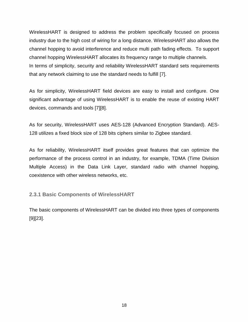
WirelessHART is designed to address the problem specifically focused on process

industry due to the high cost of wiring for a long distance. WirelessHART also allows the

channel hopping to avoid interference and reduce multi path fading effects. To support

channel hopping WirelessHART allocates its frequency range to multiple channels.

In terms of simplicity, security and reliability WirelessHART standard sets requirements

that any network claiming to use the standard needs to fulfill [7].

As for simplicity, WirelessHART field devices are easy to install and configure. One

significant advantage of using WirelessHART is to enable the reuse of existing HART

devices, commands and tools [7][8].

As for security, WirelessHART uses AES-128 (Advanced Encryption Standard). AES-

128 utilizes a fixed block size of 128 bits ciphers similar to Zigbee standard.

As for reliability, WirelessHART itself provides great features that can optimize the

performance of the process control in an industry, for example, TDMA (Time Division

Multiple Access) in the Data Link Layer, standard radio with channel hopping,

coexistence with other wireless networks, etc.

2.3.1 Basic Components of WirelessHART

The basic components of WirelessHART can be divided into three types of components

[9][23].

19

Figure 4: WirelessHART System Architecture

Referring to Figure 4, the WirelessHART field devices are used to collect the

measured data from the field then forward the data to the gateway node (sensor nodes)

and/or the field devices can receive data from the gateway in order to control the

process (actuator nodes). The field devices are normally integrated with wireless

communication, sensing and computational facilities. As mentioned above, the field

device can be either an intelligent WirelessHART device or typical (wired) HART device.

Any HART device can be easily upgraded to support WirelessHART by adding a “wired

to wireless” adapter.

The Controller, the Network Manager, and the Gateway are connected to each other

with wires (this network is usually referred as the “host network”). The most commonly

used host networks are Modbus, Profibus and Ethernet.

20

The Gateway is the bridge that enables the Controller and the Network Manager to

communicate to the WirelessHART Network. It is a device that receives sensor data

from the field instruments and forwards it to the Controller for further processing, and

sends control data to the actuators.

There is only one Gateway per network however one Gateway can have more than one

access points. All WirelessHART nodes are registered to the network through the

Gateway.

The Network Manager is an intelligent device that creates, manages and maintains the

mesh network, each node is connected directly to every other node within their

transmission range. The network manager is responsible for configuring and monitoring

the network, configuring the schedule (TDMA) and maintaining the routing tables. The

slots in TDMA schedule are allocated hop by hop based. Also, the frequencies are

allocated in those slots.

2.3.2 Medium Access Control

MAC protocol is a sub-layer of Data Link Layer of OSI model. The main responsibility of

MAC protocol is to arrange the packet transmission among multiple stations that share

the same channel.

The Design of an efficient and capable MAC protocol is crucial in wireless networks

[29]. The MAC protocol in WirelessHART is dealing with the following responsibilities:

● Providing Time Synchronization Approach

● Requesting Identification of devices that need to access the medium

● Acting as interface to transmit messages to Network Layer

● Listen to packets that are transmitted by the neighbors

21

Time Division Multiple Access

The TDMA (Time Division Multiple Access) uses schedules to allow several devices to

communicate over the network. The schedule contains different time slots to avoid the

collision problem.

The major challenges of TDMA are the time synchronization and clock drift.

In WirelessHART, the network cycle (schedule) consists of a number of superframes.

All of these superframes are created by the Network Manager and stored by each field

device. The field devices send notification to the Network Manager about the time slots

when they transmit or receive. After that, the field devices must synchronize their clocks

to permit the slot communication with neighbored devices [26].

A group of fixed length timeslots (10 milliseconds), accumulates the superframe.

A field device must be scheduled in at least one Timeslot for data transmission in a

network cycle. The slots in TDMA schedule are allocated point-to-point communication

(hopping) [25].

The frequency hopping is combined with TDMA in order to increase the reliability of the

network. The frequency hopping is used to avoid interference and reduce multi path

fading effects. To support frequency hopping, WirelessHART allocates its frequency

range to multiple channels.

The frequency range of WirelessHART is shared between 16 channels. In one timeslot

communication between two nodes can happen on any free channels. This allows

multiple transmissions happening in the same time slot between on different channels

used by different nodes.

22

Figure 5: WirelessHART Slot Timing

Referring to Figure 5, in a timeslot, the transmission of the source device starts at a

certain point, not right in the beginning of the Timeslot. This short delay allows the

source device and destination device to set up their frequency channel and allows the

receiver to start listening on the specified channel. Since, there is a delay on clocks, the

receiver must start to listen before the ideal transmission starts and continue listening

after that ideal time. After the transmission is complete, the destination device indicates

by sending an acknowledgement (ACK) to the source device to reporting success, error

or overhead [26].

The transmission in Data Link Layer uses packets to send/receive data. These packets

are called DLPDU (Data Link Protocol Data Unit Packet).

23

Data Link Packet (DLP)

This section describes the specific format of the Data-Link packet as presented in

Figure 6. The total packet length of each DLPDU (Data Link Protocol Data Unit) is 127

bytes [24]. Each DLPDU contains the following fields:

A single byte set to 0x41

A 1-byte address specifies

The 1-byte Sequence Number

The 2 byte Network ID

Destination and Source Addresses either of which can be 2 or 8-bytes long

A 1-byte DLPDU Specifies

The DLL payload

A 4-byte keyed Message Integrity Code (MIC)

A 2-byte ITU-T CRC16

Figure 6: The DLPDU packet structure

To allow MAC the transmission of packets, it has to perform a number of tasks. As

shown in Figure 7, the WirelessHART MAC protocol contains six major components:

Interfaces, Timer, Communication Tables, Link Scheduler, Message Handling Module

and State Machine. [24]

24

Figure 7: WirelessHART MAC architecture

This thesis only deals with two of the components: communication tables and link

scheduler.

● Communication tables (table of neighbors, superframes, links, and connection

graphs) are responsible for set up the communication between device and its

neighbors.

● The Link Scheduler’s responsibility is to determine the next time slot to be

allocated based on the communication schedule in the superframe table and link

table.

25

Figure 8: The communication tables

Communication Tables

Referring to Figure 8, each device maintains a number of tables in Data Link Layer.

These tables manage the communication carried out by the device and collect

information to create statics about the communication. There is four table activities:

Superframe table, Link table, Neighbor table and Graph table [24][25].

The responsibility of the Superframe table is to provide solid base for communication

between a device and its neighbors. The superframe table consists of three columns:

SuperframeID, NumSlots and ActiveFlag.

As mentioned above (section 2.3.1), the Network Manager is in charge to generate and

provide the superframes in the network.

26

The purpose of Link table is to arrange the communication between the device and its

neighbor. There can be more than one link within a superframe. A link specifies the

communication with particular neighbor or broadcast group of neighbors.

The Link table consists of five columns: LinkID, LinkOptions, LinkType, SlotNumber,

ChannelOffset.

The LinkID is the unique identification for the link, it is provided by the Network Manager

within a superframe and all entries in the table. The LinkOptions determines the

meaning of the Link; it can be either transmitter link (TX) or receiver link (RX). The

LinkType indicates the type of link (normal, broadcast, join or discovery link). The

SlotNumber is a foreign key that provides the connection between the superframe table

and the Link table. The SlotNumber represents which timeslot within the superframe is

going to be used for communication with neighbor.

The ChannelOffset represents which frequency will be used for transmission.

Neighbor table contains the list of nodes that the device can reach. Since each link has

a reference to one neighbor, the neighbor table contains the statics and properties of

itself.

The Neighbor table consists of eight columns: UniqueID, Nickname, TimeSourceFlag,

Status, TimeLastCommunicated, BackOffCounter, BackOffExponent and Statistics.

The Neighbour table has one unique key (UniqueID) which is used to connect with the

Link table.

The Nickname is a foreign key that connects to the Graph table.

TimeScourceFlag determines the device should take time synchronization from the

neighbor or not. Status determines the status information relating to this neighbor.

TimeLastCommunicated determines the last time communicated with this neighbor.

BackOffCounter decides the value of standby countdown for shared link.

BackOffExponent decides the number of back-off exponent for shared link. Statistics

contains the statistics communicated with this neighbor.

27

Graph table is used by the Network Layer and stores the routing information from

source and destination. There are three columns in Graph table: GraphID,

DestinationUniqueID and DestinationNickname.

The Graph table is maintained by the Network Manager, the information is added on

Network Layer Protocol Data Unit packet (NPDU).

The MAC protocol can use GraphID to point the DLPDU packet towards its final

destination. The Graph table has two foreign keys: DestinationNickname and GraphID.

The DestinationNickname is used to connect with the Neighbor table. Another foreign

key is GraphID as output from the Graph table to NPDU packet.

Link Scheduler

Link scheduler determines the next slot, which will be used (receiving or transmitting

slot) based on the communication schedule in the Superframe table and Link table.

In order to transmit a packet, the Link scheduler evaluates the packet that is coming

from Network Layer to the MAC protocol. MAC protocol determines the Absolute Slot

Number (ASN), which will be the Timeslot used to send the packet.

The received links contained in a superframe should be checked to determine the first

Absolute Slot Number (ASN) that can be used to receive a packet. [24][25]

2.4 Development Tools and Simulation Environment

2.4.1 MATLAB

The term MATLAB (Matrix Laboratory) covers a programming language and computing

environment for specific purpose numerical computing. Both the programming language

and the computing environment are developed by MathWorks [31]. MATLAB computing

environment provides a large set of computations for different instances in mathematics

such as matrix manipulations, statistics, numerical analysis, control theory, etc.

28

The computing environment also allows design of user interfaces and allows interaction

with code written in other programming languages.

MATLAB is used by researchers in many different disciplines starting from engineering,

science and economics.

Moreover, MATLAB computing environment also provides an additional package

“Simulink” to create graphical multi-domain simulations. Simulink package can be used

for sub tool modeling, simulating and analyzing Model-Based Design of different types

of systems.

For this thesis, MATLAB 2011b was used. The tool was provided by ABB.

2.4.2 Simulink

Simulink is a commercial tool for modeling, simulating and analyzing dynamic systems

of various domains. It is an additional package of MATLAB and it is usually included in

MATLAB [32].

Simulink was used to create the static model of the wireless and wired networks

system. To represent and build various modules in the system different types of

graphical blocks were used. Simulink allows the users the possibility to create custom

made blocks save them in “libraries” (model files) and use them in a number of projects.

Developers can customize and configure the Simulink blocks through their parameters

or programming in a MATLAB script file.

Simulink is a tool for modeling embedded and control systems, which need more

dynamic and complexity of coding for each block therefore it is a great tool for modeling

“custom made” system and it is essential in any engineering disciplines for simulating

new inventions before real life tests or observing behavior of complex systems in any

scientific field.

29

2.4.3 TrueTime

TrueTime library is a library extension of Simulink developed at Lund University. The

blocks are modifiable, discrete, MATLAB Simulink functions written in C++.

TrueTime 2.0 library was used during the implementation phase of the project. This

version of TrueTime allows designing networked control systems simulation, by using

real-time kernels blocks, network transmission blocks (wired and wireless networks). All

information here was gathered from the TrueTime Manual [10][35]. The parameters,

which are not described in the TrueTime manual, were studied through tests.

The original block library consists of the following blocks:

● TrueTime Kernel Block (programmable): simulates a node in the network. This

node simulation executes user defined tasks.

● TrueTime Network Block: acts as a communication medium and simulates the

behavior of a wired network by allowing nodes to transmit packets to each other

through this block. The internal behavior of the block is the following: the

message is taken as input from the input port that relates to the sending node,

then the message is pushed to the output port which relates to the receiving

node.

● TrueTime Wireless Network Block: simulates the behavior of a wireless

network by allowing nodes to communicate with each other through this block.

● TrueTime Ultrasound Network Block: this block simulates networks that use

ultrasound signals for communication.

● TrueTime Send Block: pre-configured node block acts as a sender node on the

network.

● TrueTime Receive Block: pre-configured node block acts as a receiver node on

the network.

● TrueTime Battery Block: this block can be used to simulate battery.

30

In this thesis, only the following nodes were used: TrueTime Kernel Block, TrueTime

Network Block, and TrueTime Wireless Network Block. Below their parameters give an

insight of how they are used.

Figure 9: TrueTime Kernel Block Parameters.

TrueTime Kernel Block has the following configuration parameters that can be set

through its Simulink Mask interface in Figure 9.

● Name of init function (MEX or MATLAB): this property refers to the MATLAB

script which contains the initialization code.

● Init function argument (arbitrary struct): the input of the initialization function.

● Number of analog inputs and outputs: determines the amount of external

analog inputs and outputs what the block possesses. The format of the input is

an array with two values where the first value is the number of inputs while the

second value is the number of outputs.

● Number of external triggers: these ports can be used to activate the block.

31

● (Network and) Node number(s): the input is an array where the first element

determines which network does the block belong to the second element

determines the ID of the node on the corresponding network.

● Local clock offset and drift: this is input again takes an array where the first

element defines a constant delay compared to the simulation time, while the

second element defines a percentage of how much the time is “faster” for the

block compared to the simulation time.

● Show Schedule Output port: allows the user to visualize schedule.

● Show Energy Supply Input port: this configuration parameter was not used.

● Show Power Consumption Output port: this configuration parameter was

unused.

Figure 10: TrueTime Network Block Parameters.

The TrueTime Network Block has the following parameters that can be set in its visual

interface in Figure 10.

32

● Network type: determines the network technology simulated by the block. The

following network types are supported: CSMA/CD, CSMA/AMP, Round Robin,

FDMA, TDMA, Switched Ethernet. Different types of networks have different

configuration parameters. In here only the general configuration parameters are

described.

● Network number: determines the ID of the network.

● Number of nodes: determines the number of nodes which belong to the network

represented by this block.

● Data rate (bits/s): determines the speed of the network.

● Minimum frame size (bits): determines how long the smallest possible

message frames are.

● Loss probability (0-1): determines the chance of a message not arriving to the

receiving node.

● Initial seed: The numbers of variables which can put the network block in a

random state.

● Show Schedule Output port: allows the user to visualize schedule.

TrueTime Wireless Network Block has the following parameters that can be set in its

visual interface in Figure 11.

● Network type: determines the network technology simulated by the block. The

following network types are supported: 802.11b (WLAN), 802.15.4 (Zigbee),

NCM_WIRELESS

● Network number: determines the ID of the network.

● Number of nodes: determines the number of nodes which belong to the network

represented by this block.

● Data rate (bits/s): determines the speed of the network.

● Minimum frame size (bits): determines how long the smallest possible

message frames are.

● Transmit power (dbm): determines the range of the network.

33

Figure 11: TrueTime Wireless Network Block Parameters.

● Receiver signal threshold (dbm): minimum signal strength that the receiver

can detect.

● Pathloss function: user defined path loss function.

● Pathloss exponent (1/distance^x): determines how fast the signal gets weaker

in the transmission environment.

● ACK timeout (s): determines how long the sending node waits for the

acknowledgment of the receiver, before it considers the message lost.

● Retry limit: the maximum number of retransmissions allowed.

● Error coding threshold: determines the limit of errors when decoding signals.

34

● Loss probability (0-1): determines the chance of a message not arriving to the

receiving node.

● Initial seed: determines the pattern of randomization that is used to put the

network block in a “random” state.

● Show Schedule Output port: allows the user to visualize schedule.

● Show Power Consumption Output port: allows the user to visualize power

consumption.

One disadvantage is that the separate blocks cannot truly be tested by themselves. In

case of a complex system, looking for problems in separate blocks can cause some

delay.

It is necessary to initialize kernel blocks, network blocks, to create tasks, interrupt

handlers, timers, events, monitors, etc. before executing the model. The initialization

code and the code that is executed during simulation must be written in MATLAB or

C++ programming language.

Another disadvantage is the absence of resources such as supporting documents and

examples. There is a manual, but it is unclear, in some places outdated, and unfinished.

35

3. ABB’s WirelessHART Tool

The ABB’s WirelessHART Tool was developed in order to ease and speed up the

process of creating simulations. The first version of WirelessHART Tool allowed the

users to generate models to simulate a single WirelessHART control network, add and

remove nodes to the network, set up a simple schedule for communication and set up a

single PID controller to control all the processes

Before the development of the WirelessHART Tool began, there had been a major

project to build some static WirelessHART simulations in MATLAB and Simulink and

add WirelessHART support to TrueTime.

3.1 TrueTime Upgrades

This section describes how the WirelessHART has been implemented in TrueTime by a

group of ABB’s researchers. Since this thesis was not dealing with changing or

extending TrueTime, the TrueTime library was only explored briefly. However there are

a couple of upgrades that need to be mentioned.

The WirelessHART MAC protocol has been developed with C++ functions together with

MATLAB MEX-interfaces. The MEX-interface is an adapter between C++ and MATLAB.

The MEX interfaces of the Blocks are connected to the Mask Interface of the Blocks.

[33] All the information which is required to simulate a WirelessHART network can be

entered on the mask, but not all data is used by functions, thus not all WirelessHART

features work correctly.

36

3.1.1 TrueTime Network Block

Figure 12: New fields in the TrueTime Wireless Network Block Mask, supported Multi-Channel

● Fixed Packet Loss, Time Array(s): when the box is ticked user can enter (in the

Time Array) the beginning and the end of one or more time interval(s), during

which all the packets sent on that network are lost.

● Noise Average (dBm): determines the average disturbance on the network.

● Noise Variance (dBm): shows how much the disturbance can differ from the

average.

● Number of Channels: defines how many channels can be used for

communication on the network.

● Slot Size (s): determines the length of one Time Slot (0.01 s for WirelessHART).

● Superframe Size (n. Slot): determines the number of slots contained in a

superframe.

37

3.1.2 TrueTime Kernel Block

Figure 13: New fields in the TrueTime Kernel Block Mask, supported Multi-Channel

● WirelessHART Device check box: determines whether the WirelessHART

parameters of the node are available or not.

● Frame ID: determines which message is sent/received on which Superframe.

● Time Slot: determines which Timeslots are used for sending/receiving

messages.

● Channel Offset: determines which channels are used for sending/receiving the

messages.

● Destination Device: determines the origin/recipient nodes of the messages.

● Link Option: determines whether the message is received by the node or sent

from it.

38

● Link Type: determines whether a link is normal, shared or advertised.

Implementation of Device Communication Tables

As mentioned in the background (section 2.3.2), the TrueTime has been modified based

on the WirelessHART MAC protocol theory. The Devices Communication Tables

together with Mask interface of TrueTime Kernel block have been implemented in order

to support all communications [25].

FrameID TimeSlot ChOffset DevAddress LinkOpt LinkType

{1…

Nbrframes}

{1…NbrSlots} {1…Nbrch} {1…NbrNodes} 0 = RX

1 = TX

0 = normal

1 =

advertisement

-1 = shared

Table 2: Logical Device Tables in Upgraded TrueTime.

The information of the device table contains six columns: FrameID, TimeSlot, ChOffset,

DevAddress, LinkOpt and LinkType.

● FrameID: indicates the unique identification number of a Superframe. Each

WirelessHART device supports multiple Superframes.

● TimeSlot: contains a list of slots where the device needs to communicate.

● Channel Offset (ChOffset): determines in which channel that the device use to

communicate in particular Timeslot.

● DevAddress: indicates the destination device that will receive the transmission.

● Link Option (LinkOpt): determines two types of communication: RX (0) and TX

(1). The zero (0) value means that the device must receive, while the one (1)

value means that the device must transmit.

● LinkType: indicates the link types of slot, the slot can be either reserved, shared

slot or dedicated.

39

Implementation of Time Synchronization

In order to achieve and fulfill an efficient TDMA communication technique, the time

synchronization of clocks between devices in the network is critical. This is because

each device has their local clock. This allows during the synchronization of two stations

that each one should be able to estimate the local time of each other. [25]

When TrueTime was upgraded, the above described problem was taken into account

and the MAC protocol was modified based on ASN (Actual Slot Number) technique to

find the actual Timeslot for sending and receiving messages.

In the implementation, the device reads the actual simulation time from the MATLAB

environment, and then the actual simulation time value is used to compute the actual

Timeslot using the following formula (3.1.2):

(3.1.2)

where the exectime is the execution time of the active device. The Slotsize is fixed to 10

ms in WirelessHART. The SuperframeSize is the number of slots contained in a

Superframe.

40

3.2 Application Structure

Figure 14: Application Structure Design

Referring to Figure 14, the structure of the application does not follow any conventional

software engineering structure or architecture. It was decided that in order to show the

application structure the uses structure must be displayed.

The uses structure uses the “requires the correct presence of” relation between the

elements of the structure, thus shows which elements need which other elements in

order to function as expected. The arrows represent this relation on the diagram

[20][21].

The diagram uses UML (Unified Modeling Language) notation.

41

7 main elements build up the application structure. These elements are defined through

code inspection, research and testing.

GUI: The purpose of the GUI is to allow users to set up different simulation scenarios

fast and without getting lost in the details. The UI creates 17 global variables for

communication between different functions. These global variables store data about the

transmission schedule and the nodes in it.

Generic Model: is a saved Simulink model. The Generic Model is used as template

when generating the simulation model. Generic Model contains TrueTime blocks such

as TrueTime Kernel Blocks, TrueTime Wireless Block, etc.

An advantage of generic model is to allow changing basic structure quickly without the

need of coding.

WHART Library (whart_lib): is a saved Simulink Model that stores an important

TrueTime Simulink blocks that are used to build the simulation model. These blocks are:

Actuator block, Sensor block, the Position block and Intermediate block. When

generating the simulation model the WHART_lib is opened and the required nodes are

copied into the simulation model.

Simulink: is a MATLAB extension and library. It is used to take general purpose blocks

into the model and is responsible running the general simulation mechanism.

Structure Organization

Both the Generic Model and the WHART_lib were constructed from blocks that can be

found in Simulink as well as blocks from the TrueTime library. The Sensor, Actuator,

Intermediate, Controller and Gateway Blocks are special from the viewpoint that they

are programmable using MATLAB Script Files (this connection is not shown on the

diagram because it is dynamic). These Script Files implement functions in order to

determine the runtime behavior of the blocks.

42

During runtime, the Script Files are using the global variables created by the UI in order

to determine what behavior they should simulate (connection is not shown because it is

dynamic).

The TrueTime library uses some building blocks from the Simulink library as well as, so

called S-Function (System-function) files. The S-Function files are compiled files that

are included in the library itself that is why the authors choose not to display them. [33]

3.3 User Interface & Functionality

WirelessHART GUI (Graphical User Interface) was created using GUIDE (GUI

Development Environment of MATLAB). GUIDE is a tool for designing and

programming GUIs.

GUI components are building blocks of the GUI. Each GUI component has its own

callback. The “callback” is a function that developer can implement and connect to the

specific GUI component. The callback controls the GUI or component behavior by

performing a task or action.

The callback is activated by an event of its component. An event is a previously defined

user interaction with the GUI component.

There are several callbacks provided by GUIDE, for example ButtonDownFcn,

KeyPressFcn, Callback etc. [12]

For instance, the Delete Button is the GUI component. The Delete button uses

“Callback” as its callbacks property type. The “Callback” is one kind of a callback

property. In this case, the Delete Callback will be activated when the user pushes the

Delete Button. Whenever the Delete Callback is activated, the function code contained

by the delete callback will be executed.

As shown in Figure 15 and 16, the components and their functions were grouped on the

GUI considering their purpose. For grouping the components on the GUI panels were

used [11][13].

43

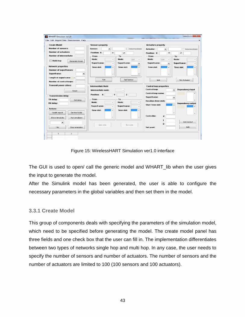
Figure 15: WirelessHART Simulation ver1.0 interface

The GUI is used to open/ call the generic model and WHART_lib when the user gives

the input to generate the model.

After the Simulink model has been generated, the user is able to configure the

necessary parameters in the global variables and then set them in the model.

3.3.1 Create Model

This group of components deals with specifying the parameters of the simulation model,

which need to be specified before generating the model. The create model panel has

three fields and one check box that the user can fill in. The implementation differentiates

between two types of networks single hop and multi hop. In any case, the user needs to

specify the number of sensors and number of actuators. The number of sensors and the

number of actuators are limited to 100 (100 sensors and 100 actuators).

44

Until the model is generated, all other functionalities of the UI are restricted. The

Intermediate Panel, the Actuator Property Panel’s components which are responsible

for scheduling data transmission and the Sensor Property Panel’s components which

are responsible for scheduling data receiving, are only enabled if the user selects the

multi hop communication option. The WirelessHART Simulator allows the sensor and

actuator nodes to act as intermediate node when the multi-hop communication is

enabled.

There is a difference between how the UI counts the nodes and how the Simulation

model numbers them.

In Simulation model all the node IDs use the same numbering, while the UI splits them

by functionality to Sensor nodes, Actuator Nodes, Intermediate Nodes, Gateway and

Controller. The solution to the problem is presented here:

The Sensor nodes from the UI come first, the Actuator nodes come second, The

Intermediate nodes third, then the Gateway and finally the Controller, when the

numbering of nodes in Simulation model. For example, in case of: there are 3 Sensors,

2 Actuators, 1 Intermediate. In Simulation model the Sensor nodes number are the

nodes from 1-3, the Actuator nodes are 4 and 5, Intermediate Node is 6, Gateway is 7

and Controller is 8. [11]

3.3.2 Network Property

After generating the model, the user can proceed to the Network Properties Panel. On

the Network Property Panel the user can assign the network properties such as number

of superframes, length of superframes, number of control loops and transmit power of

the network.

The Superframe Number property determines how many superframes are in use on the

WirelessHART network.

The size of a superframe must be multiples or common divisors of each other. The

reason for this is a common real-time scheduling problem that they must be compatible

on a longer timescale.

45

The Number of Control Loop field determines how many control loops are run by the

Controller.

The Transmit Power is used to determine the strength of the transmissions signal. The

transmit power will be defined at 10 dbm as a default if not specified.

The Reset button in Network Property panel is used to clear all options on the GUI, and

allows the user to generate a new model.

This network property will be enabled only after the model is generated, generated_flag

global variable is used to check whether the model is generated or not.

The Superframe is a global variable (array in this case), with the length of 1 which is

changed accordingly to Length of Superframe field. If the value in the Length of

Superframe field is incorrect, the user is not allowed to set the Control Loop number.

3.3.3 Sensor Property

Sensor Node: primarily these nodes only send data. When Multi Hop is enabled, the

sensor nodes can act as intermediate nodes thus send and receive data.

Through the Sensor Property panel the user can determine in when a specific sensor

sends data and in which superframe. First, the user must select the desired sensor from

the drop-down list. The user can also assign a specific name for the signal of each

sensor. The X-Y-Z position is used to set the position of the node in a 3D space. This

3D coordinates are used to compute the area where the signal can be received from

that node.

The “Set Sensor” button is used to store the values of the sensor in the virtual tables of

the UI and the sensor also appears on the Schedule Table of the UI.

The “Edit button” removes all information of the sensor from the virtual tables of the UI

and also deletes it from the Schedule Table of the UI from the scheduler table and clear

the sensor table.

In case of single hop communication all sensors send data directly to the gateway, thus

only the gateway node will visible on “To” drop-down list.

In case of multi-hop communication the “To“ drop-down list the receiving node can be

selected by the user.

46

3.3.4 Actuator Property

Actuator Node: primarily these nodes only receive data. When Multi Hop is enabled, the

actuator nodes can act as intermediate nodes thus send and receive data.

The Actuator Property panel is almost identical to the Sensor Property panel. The only

difference is that when the user does not use multi hop communication, all of the

actuators receive the data from gateway, thus the “GW” node will be the only option on

“From” panel.

3.3.5 Intermediate Node

Intermediate Node: these nodes can only be used when Multi Hop is enabled. They can

both send and receive data.

The Intermediate Node panel is only enabled if the multi-hop option was checked in the

before generating the model.

The GUI components included in this panel are identical to those in the “Sensor

Property” and “Actuator Property” panels as well as their purpose.

3.3.6 Control Loop Properties

In the control loop panel, the user is able to select the desired control loop and set

various properties for it.

The name of the control loop can be specified in a control loop name field.

The user must set the timeslot and the superframe of control loop.

The Duration determines how much time (measured in timeslot) the process will require

for completing the calculations. The default value of duration is 1 timeslot.

Each control loop has separate PID control values and a Setpoint that the user can

assign. The default PID control values are P=10, I=0, D=0 respectively. The default

setpoint is 1. The dependency input and output show which sensor and actuator is

related to the currently selected control loop. The user can assign more than one sensor

and/or actuator for the selected however only the most recent ones are displayed.

47

The control loop properties will be stored in the virtual tables and displayed on the

WirelessHART Tool UI after the “Set Control” button was pressed.

The “Edit” button clears the selected control loop from the virtual tables as well as from

the UI.

3.3.7 Transmission Delay

WirelessHART tool simulator can simulate the transmission delay for the host network.

The Transmission Delay panel provides two types of delay: TX delay (Transmit), RX

delay (Receive). The default value of both TX and RX delay is zero and the maximum

value of each of them cannot exceed 0.005 second.

TX (Transmission Delay) functionality is implemented to provide a time delay when

transmitting the data from the Controller to Gateway. On the other side of the Controller,

RX (Receive Delay) functionality is implemented to provide a time delay when receiving

the data from Gateway to Controller.

3.3.8 Actions

The actions panel contains five different functionalities: Health report, Set the model,

Show timeslots, Run/ Stop Simulation and Plot.

After all nodes (sensor, actuator, intermediate) properties and control loop property are

set, the user can verify and check the schedule of the whole network Using the “Health

Report” button. The Health report provides the several errors and warnings if something

is incorrect in the schedule setup.

The simulation cannot be started if there is the error or warning in the Health report.

In case the settings are correct, the displayed message says “Scheduling successful”.

The “Show Timeslots” button is built in order to refresh the Schedule Table on the UI.

48

The “Set the Model” button is used to copy all node parameters and values from the

virtual tables into the Simulink Model. The model cannot set those values into the model

if there are any warnings or errors in the Health report. If the user does press the “Set

the Model” button while there are still error(s) in the schedule, a dialog box will appear

warning the user that there are still errors.

“Run/Stop Simulation” buttons are used to control the when simulation should start and

stop. The user can see the simulation time displayed on the UI in seconds.

Above the “Plot” button there is an “actuator drop-down list”. The user can chose from

this list which actuator’s results they wish to plot.

The “Plot” button is used to display the results of the previously ran simulation. There

are two plot windows appearing. The first plot window shows the actuator output, the

second window shows the plant output and the setpoint. Both plots correspond to the

drop-down list above where the user can select the process for display.

3.3.9 Schedule Table

The Schedule table is used for displaying the current schedule of the WirelessHART

network. There is no interaction possible with the UI component however it does display

warnings when collisions occur.

3.3.10 Menu

3.3.10.1 Import and Export

The WirelessHART Tool also allows the users to import saved and export the generated

Simulink model and network configuration from/ to excel sheet.

3.3.10.2 Add and Remove node

The Add and Remove node menu allows the users to add or remove node(s) from and

to the network.

49

3.3.10.3 Retransmission

The retransmission is a separate option, placed on the menu. The WirelessHART tool

allows the users to retransmit messages in empty Timeslots.

3.4 Simulation Model

This section describes the block organization of the simulation model, the internal block

architecture of Sensor, Actuator and Intermediate blocks as well as the properties of the

included Simulink blocks [34].

The block organization shows the interconnections between the blocks and how the

data is transmitted and received on the entire network in Figure 17.

Figure 17: The completed Simulation Model of WirelessHART Tool

Blocks

The Network block (WHART_NET) contains several parameters as shown in TrueTime

section. The Loss Signal output and Schedule output allow the users to plot the Packet

50

Loss of the network and the schedule of each node. The Network block is attached with

Position block.

The Position block contains the physical location (X, Y, Z) of nodes that belong to the

network as well as the noise of the environment of the particular node. The users can

specify the physical position of each node in the network through the WirelessHART

Tool interface. In case of the noise, the value will be zero (0) constant since the UI does

not have options to set or change it.

Gateway block (Gateway) is connected to Control block (Control) using an analog

output. Between them, a delay block can be found. The Gateway block has one input

port and two output ports. The Gateway schedule output is provided by TrueTime, in

case of studying the Gateway behavior.

RX Delay, as shown in the Figure 17, is the Receiving Delay block. The RX_DL block

can be specified by the users through the WirelessHART Tool interface.

The Control block has two input and two outputs. The two inputs are combined with

“Mux” block that converts several input signals into a vector.

Two block interface ports (output) are similar to Gateway block’s output ports. The first

output interface uses Digital to Analog converter of TrueTime to transmit the data to

Gateway block. The second can be used to plot the schedule of the block.

The Reference is a Constant block from Simulink. This block generates a constant

value. The users are able to set the Reference value through the Setpoint field of the

Control properties panel of the GUI (#6).

TX Delay contains the functionality of Transmission Delay is similar to RX_DL, but

TX_DL is performed when the analog signal is transmitted to Gateway.

PID block processes the incoming data and then forwards the results to Gateway block.

On default, the PID is chosen to be discrete-time. The internal parameters of PID

51

consist of Proportional value, Integral value, Derivative, Sampling Time and Filter

Coefficient. The value of the Filter Coefficient is 0 on default, and the Sample Time is

0.01s on default. The GUI makes only the P, I and D values available for input.

The simulation time of the model is controlled by a group of Simulink blocks which are:

Clock Simulink, Sink Display Simulink and “to Workspace” Simulink (sim_time) blocks.

Clock block controls the current simulation time. The length of simulation time runtime

can be specified by the users in the Simulink run-time interface. The simulation time in

default set as “inf” which means the simulation will run until the users stops it.

Display block shows the value the input from the Clock Simulink block.

sim_time block is used to write the signal data to MATLAB workspace. When the

simulation is completed or paused, all data created by the simulation is written to the

workspace. The users can specify how to save the data, from several formats such as

time-series, array, structure and structure with time.

Plant refers to “Transfer Fcn” Simulink block is used as a “Plant” for processing and

transforming the data. The Transfer Fcn has two parameters: Numerator coefficients

and Denominator coefficients. The Numerator coefficients and Denominator coefficients

can be a vector or matrix expression. The default transfer function is the following

formula (3.4):

(3.4)

The default of Numerator coefficients is one (1) and Denominator coefficients is [1 1].

Actuator block can be expanded to see how it is built from sub-blocks as shown in

Figure 18. The Internal architecture of Actuator Sub-blocks consists of one TrueTime

Kernel block and three Simulink blocks.

52

Figure 18: The completed Simulation Model of WirelessHART Tool with Actuator Sub-blocks

The TrueTime Kernel block represents the core of the actuator node. This core has two

output ports. The D/A output port is connected to the Actuator output scope and the to

the Plant through “Outport” Simulink block, while the Schedule output port is connected

to the “Act sch” scope.

The connection from D/A to A/D acts as a feedback (buffer). This connection is only

used when the Actuator block is used as Intermediate node.

Sensor block receives the data from the “Plant”. When expanded it is discovered that

the block contains an Inport, a Constant block, a TrueTime Kernel block and two scope

blocks as presented in Figure 19.

53

Figure 19: The completed Simulation Model of WirelessHART Tool with Sensor Sub-blocks

The Constant Simulink block called “Set” represents the value of the control setpoint.

One scope plots the Plant output and the setpoint of the control loop while another

scope displays the sensor’s schedule on the network.

In case of the sensor is used as an intermediate node, the sensor node sends data

backwards to A/D input.

Intermediate block does not have input or output port from its high level view. The

“buffer” acts as a feedback the same way as it does when the actuator or the sensor

nodes are used as intermediate nodes.

Block Organization

The simulation model was generated based on the input of the user, through GUI such

as number of sensor, number of actuator, etc. The Figure 17 shows the completed

simulation model of WirelessHART tool with one Wireless Sensor and one Wireless

Actuator. The Network block is attached with Position block.

54

Two incoming inputs to Control block are Analog to Digital input from Gateway and

Reference (setpoint). Between the Controller and the Gateway blocks, the TX_DL and

the PID blocks can be found.

The Gateway block transmits the data through the Digital to Analog Converter (D/A) port

of the Kernel TrueTime block to the Control block. RX_DL is the Receiving Delay block;

this block is organized in between Gateway block and Control block towards the

delaying of receiving data.

3.5 Code Readability

The code for the functions of the UI was included in one MATLAB script. There is also a

lot of repetition in the code, meaning that whenever two functions are have some

common code it is copied and pasted in both.

All the project files are included in one folder. Since there are a lot of files that are used

during runtime, it becomes very confusing to navigate inside the folder.

The above described, style of code writing prevents from the application to

accommodate good maintainability, extensibility, changeability and response time. The

style of code writing also goes against pragmatic programming: Don’t repeat yourself,

File and Folder Organization, Avoid Deep Nesting [4].

55

4. Extensions to WirelessHART Tool

This section provides requirements specification. These requirements were requested

by customers in order to improve the capability of the tool. The limitations of the thesis

can be found in this section.

4.1 Requirements

4.1.1 Wired actuator

The customer needs the WirelessHART Tool to be able to simulate control systems

where the actuators are wired and the sensors are wireless.

4.1.2 Multiple Channels

The purpose of utilizing Multiple Channels is to enable devices to split the frequency

range of the network into multiple channels. These channels covering different

frequencies can allow the nodes to communicate simultaneously.

The customer needs the WirelessHART Tool to allow users to generate networks that

use multiple channels in their frequency range to transmit data.

4.1.3 Toggle switch for sensor, actuator, intermediate panel

The WirelessHART tool displayed three different panels together on the GUI: sensor,

actuator and intermediate panel. This approach resulted that the user interface was and

difficult to follow, especially considering that each panel had similar configuration panel

such as nodes selection, time slots selection, edit and delete nodes button and etc.

56

4.1.4 Using the same color pattern for each control loop

The customer wanted to be able to see which sensors, actuators, and control loops

belong to the same control loop on the schedule table. The solution was to give the

same color to these entities in the schedule if they belong to the same control loop.

Note that intermediate nodes are in our consideration due to they do not belong to any

specific control loop.

4.1.5 Remove node on scheduling table by using Delete Key

One of the customer’s wishes was to be able to delete nodes from the schedule by

selecting them in the schedule and deleting them using the “Delete” key.

4.1.6 Improving the correctness of Controller

There were several demonstrations for the customer when the simulation mechanism of

the controller was discovered to be incorrect. Some of these problems were solved as

part of the thesis and others were too complex and not considered in the scope of this

work.

It was discovered that the block organization of the PID controller and TX_DL was

incorrect. The on the way from the Controller Block the PID has to come first, then the

TX_DL and then the Gateway.

Another problem was that only one PID was used to calculate for all the actuators. After

a short discussion, it was decided that one PID is to be added for each actuator.

When testing with different schedule combinations, some of them produced unexpected

and incorrect results. In order to identify the problem the code was inspected and it was

found that the gateway does not know what data is to be sent to which node.

Since in the simulation the user acts as the Scheduler, it was obvious that when they

57

create the schedule they know what data is to be sent to which node. Consequently, the

user needed to have more control over the Gateway.

4.2 Limitations

4.2.1 Internal Limitations

These limitations define what is excluded from the scope of the thesis by the authors

with the consent of the customer.

● The redesign of the software architecture was out of work’s scope.

● The thesis did not address perfecting the controller.

● The thesis did not address modifying the TrueTime library.

● The above mentioned reasons set limitations in extra-functional requirements:

execution speed, extendibility, modifiability. The thesis did not focus on improving

any of those.

4.2.2 External Limitations

These are the limitations that could not be controlled by the authors.

● TrueTime does not support multiple channels.

58

5. Solution

This section presents the appropriate solutions for the requirements in section 4. The

descriptions contain the choices the authors made and the reasons for those choices. It

is also shown how the problems solved, based on what the authors have learned during

their research.

The upgrades of WirelessHART Tool architecture, GUI, and Simulation Model are

described here in order to give a better understanding of the changes.

The section is broken to subsections using the same organized paper as in Section 3.

The subsections only describe the new functionality to allow easier comparison between

the new and the old WirelessHART Tool.

5.1 Application Structure

The Application Structure Design has not been changed because of time limitation and

customer’s request. For the existing application structure, please see Section 3.2.

It was decided to follow the existing application structure and utilize its elements as a

means to avoid any effects on the existing functionality of WirelessHART tool.

The new functionalities were mapped carefully on the existing elements of structure

then implemented to avoid adding extra elements and to avoid complicating the

structure.

5.2 User Interface Design

This section presents the description of upgrades made on the GUI. The GUI was

reorganized in order to accommodate the required changes as presented in Figure 20

and 21.

59

Figure 20: New WirelessHART Tool User Interface.

5.2.1 Changes in Create Model

Wired Actuators

There were two new items added on the panel, both dealing with the wired actuators.

The wired actuator checkbox has been added because there are major differences in

what the Simulation model includes with and without the wired actuators.

The number of Wired Actuators has been separated from the number of Wireless

Actuators because during when setting the model and during simulation, it would be

difficult to track which node has what number on what network in the model and in the

Global Variables.

5.2.2 Changes in Sensor/Actuator/Intermediate Property

Toggle buttons

60

The chosen solution to the above described problem is to place toggle buttons each

node property (Sensor, Actuator and Intermediate) which display only one panel at a

time. This allows the user to follow easier what is happening when setting up the

simulation. For example, if the user is focusing on sensor configuration, the user would

click at the sensor toggle switch, and then only the sensor configuration panel would be

displayed.

The toggle buttons were selected to separate one big panel of Sensor, Actuator and

Intermediate.

The concept is to split the big panel into small panels. The panels are controlled by the

three toggle buttons. The starting point will be clear panel, unless the user clicks on any

buttons. The sensor panel will appear when the users click on Sensor toggle button. If

the users click on Actuator toggle button, the actuator panel will appear on the UI.

The controller panel was not included between the toggles because it does not belong

to the network nodes.

Multiple Channels

It was discovered that TrueTime library does not fully support the use of multiple

channels communication. TrueTime’s mask interface is prepared by the channel offset

input field, however it only gets the input data, but there is no function connected to

process or use that data.

After discussing with the customer, the customer’s wish was to design to prepare the

WirelessHART tool for supporting multiple channels, in case the functionality would be

added in TrueTime. This meant updating the user interface for selecting the channels,

adding a new global variable where channel communication is stored, and implemented

algorithms to display the multiple channel communication in the Schedule Table and to

verify the schedule.

Thus, the logical idea for multiple channels was built on top of the GUI. The concept

was to add a dropdown list element for each node devices (Sensor, Actuator,

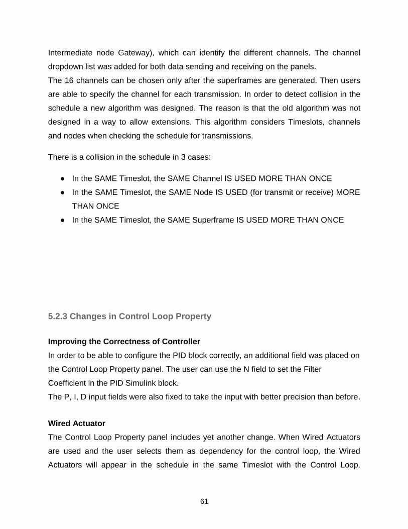
61

Intermediate node Gateway), which can identify the different channels. The channel

dropdown list was added for both data sending and receiving on the panels.

The 16 channels can be chosen only after the superframes are generated. Then users

are able to specify the channel for each transmission. In order to detect collision in the

schedule a new algorithm was designed. The reason is that the old algorithm was not

designed in a way to allow extensions. This algorithm considers Timeslots, channels

and nodes when checking the schedule for transmissions.

There is a collision in the schedule in 3 cases:

● In the SAME Timeslot, the SAME Channel IS USED MORE THAN ONCE

● In the SAME Timeslot, the SAME Node IS USED (for transmit or receive) MORE

THAN ONCE

● In the SAME Timeslot, the SAME Superframe IS USED MORE THAN ONCE

5.2.3 Changes in Control Loop Property

Improving the Correctness of Controller

In order to be able to configure the PID block correctly, an additional field was placed on

the Control Loop Property panel. The user can use the N field to set the Filter

Coefficient in the PID Simulink block.

The P, I, D input fields were also fixed to take the input with better precision than before.

Wired Actuator

The Control Loop Property panel includes yet another change. When Wired Actuators

are used and the user selects them as dependency for the control loop, the Wired

Actuators will appear in the schedule in the same Timeslot with the Control Loop.

62

However, since they are on different network (with different communication mechanism)

it is not entirely true. Since the Ethernet Network is much faster than the WirelessHART:

on the Ethernet in a timeframe of 10 millisecond, and more than 400 messages (with

the same size as in WirelessHART) can be sent. The authors of this thesis assumed

(and got permission from the customer) that the difference in communication could be

overlooked.

5.2.4 New Gateway Panel

Improving the Correctness of Controller

The Gateway panel was added into the new GUI in order to solve the problem of

knowing destination device when the gateway transmits data to an intermediate node.

The cause is that the Gateway does not know what register to take the data from in

case it is not sent directly to the destination node.

This solution was created because this allows the user to fully take control of the data

transmission.

The Gateway panel has similar properties to sensor and actuator panel properties. The

only different feature is the users are able to specify which actuator will be the using the

data that is sent. The Gateway panel only appears if intermediate nodes are allowed.

There was one global variable added to resolve the problem.

5.2.5 Change in Schedule Table

Using the same colors for each control loop

The following solution was used to fix the colors in the schedule. The color of control

loop is generated by randomized number of RGB pattern, Red Green and Blue main

pattern, from 0 to 255 bit pattern of each main color. The idea is to identify unique color

for process and color the belonging sensor, actuator node and control loop to the same

color.

63

The randomized functionality was used to generate 256 random numbers, between 0 -

255. The reason for this is that in the WirelessHART specification, one network can

have only 250 nodes, and there are fewer possibilities to generate the same color for

each group of sensor - control loop - actuator.

In order to show the color, the color tag is applied into a cell in scheduling table. The

color tag needs to be defined by a color name or in RGB code. The RGB code is more

efficient as means to identify many colors. The RGB code represents three variables,

each variable contained by number in between 0 - 255.

After the random numbers were generated, they were stored in different variables

representing R, G and B. Then, the containing variables are put as the color tag. For

example, rgb(x,x,x) function contains R = 0, G = 0, B = 0, this represents rgb(0,0,0)

which means black color.

Delete Key

In order to provide a more visual way to remove transmissions from the schedule, an

alternative way is provided, where users can select the desired transmission on the

Schedule Table and remove them by pressing the “Delete” key.

The CellSelectionCallback is used to get the right row and column of selected cell on

the table. The Delete Key button is represented by number of “127” in ASCII number. In

the event of the Delete Key is pressed, the specified row and column of that cell will be

read in order to check what node is in inside that cell, and remove them from the

corresponding tables.

Multiple Channels

The Schedule Table’s Cell format for was changed in order to show what channel the

transmission is taking place on. The channel number was prefixed before the nodes of

the transmission and given the same color as the transmission.

64

5.3 Simulation Model

Improving the Correctness of Controller

On a real WirelessHART network the Gateway and the Controller use registers for

exchanging data. The Gateway knows which register belongs to which sensor on the

input side of the controller; the Controller knows which input register to read from and

which input register to write to, for each Control Loop, then the Gateway knows again

which transmission (towards the actuators) will use which register (controller output)

data.

The previous version of the model did not consider registers on the Gateway and the

Controller. This resulted that when the simulated network had many sensors and

actuators, as well as many control loops, the schedule had to be very specific in order to

work.

The problem was that both the Gateway and the Controller blocks had only one analog

input where messages arrived.

For example when there are two control loops with the following dependencies:

CL1: Sensor1, Actuator1

CL2: Sensor 2, Actuator2

65

Figure 22: Simulink Model of both Wireless Sensor and Wireless Actuator

The transmissions of control loop order of each control loop must not be mixed:

Timeslot 1 Timeslot 2 Timeslot 3 Timeslot 4 Timeslot 5 Timeslot 6

S1->GW CL1 GW->A1 S2->GW CL2 GW->A2

Table 3: Example of Schedule table

In the schedule seen above, Table 3, we can change the patterns (control loop +

transmissions) of the whole control loop with the other but we cannot change the

individual transmissions or control loops place in the schedule. For instance if we put

GW->A2 in Timeslot 3 and GW->A1 in Timeslot 6 instead, the output of both processes

would be incorrect.

66

In order to simulate registers we have decided to use analog connection.

Referring to Figure 17 in section 3.4, where the PID block was organized after TX_DL

block, this method created some confusion and after short discussion, it was decided

that that PID should come before the TX_DL as in Figure 22. The reason was that the

delay before the PID controller might distort the calculation of the PID. Another reason

was that the PID and the Controller block were supposed simulate the control together,

while the delay was used to simulate the delay on the way back from the Controller to

the Gateway.

During the investigation, other problems were found such as single PID served all the

control loops. The PID controller block “remembers” old data, in case of one PID and

more than one control loop this leads to the controller working ineffectively and

incorrectly.

The simulation model has been changed according to the single PID controller problem

by adding the number of PID controllers in accordance with number of actuators. After

the PID controllers are generated, they are connected to a “Mux” and a “Demux”

Simulink blocks.

In order to improve the PID controller behavior, the new parameters inside PID

controller block were changed based on customer requirement. The Sample time of PID

controller was not changed.

The solutions in the controller might also raise some issues; however the Controller is

“more correct” then the previous. It needs to be mentioned that there were a number of

solutions considered for the problems and all of them had their defects.

67

Figure 23: Simulation Model of Wireless Sensor and Wired Actuator

Wired Actuator

As shown in the Figure 23, this model was created as a means to determine the

requirement of Wired Actuator (section 4.1.1).

In the real world, the Actuator can be either Wireless Actuator or Wired Actuator. The

previous stage of WirelessHART tool did not consider this functionality. So, in this thesis

we extended an advance communication of two networks coexist. The purpose was to

investigate and evaluate the performance of the data transmitting though both networks.

The first network is WirelessHART and is responsible for communicating data from

sensors to controller through a gateway. The second network is wired, it uses Ethernet

(CSMA/CD) protocol and this network is responsible for communicating data from the

controller to actuators. The Wired actuators were requested to appear in the schedule.

68

The in the real plant the wired actuators will use a PROFINET solution, however the

implementation of PROFINET in TrueTime makes it quite difficult to automate the

generation of such network. Since the primary objective of this tool is to simulate

WirelessHART networks, it was decided that PROFINET would not be used.

FDMA was another considered solution, but it was dropped since its behavior was not

suitable.

TDMA had quite unclear description in the TrueTime manual about how the static

schedule is to be used, so it was decided to move forward with another solution.

The Ethernet (CMSA/CD) network was chosen to interact with WirelessHART network

in the system because of simplicity in implementation and well matching behavior with

the WirelessHART.

In case of sensor node is Wireless and actuator node is Wired, the Wired Actuator block

will be copied into the Simulation Model instead of Wireless Actuator block. The Figure

23 shows the different block organizations of Simulation model when actuator is Wired.

There are three important blocks that are added in this Simulation model: Wired

Actuator block, Ethernet Network block and ControllerBUS block.

The Wired Actuator block is connected to “Plant” and send the data over the “Outport”

Simulink block. The internal block design of Wired Actuator block is similar to Wireless

Actuator block. The Wired Actuator could not be used at all on WirelessHART Network

thus no uses such as intermediate node behavior scenario. Therefore, there is no

feedback from output port coming into the input port. The feedback output is terminated

by using the “Terminator” Simulink block.

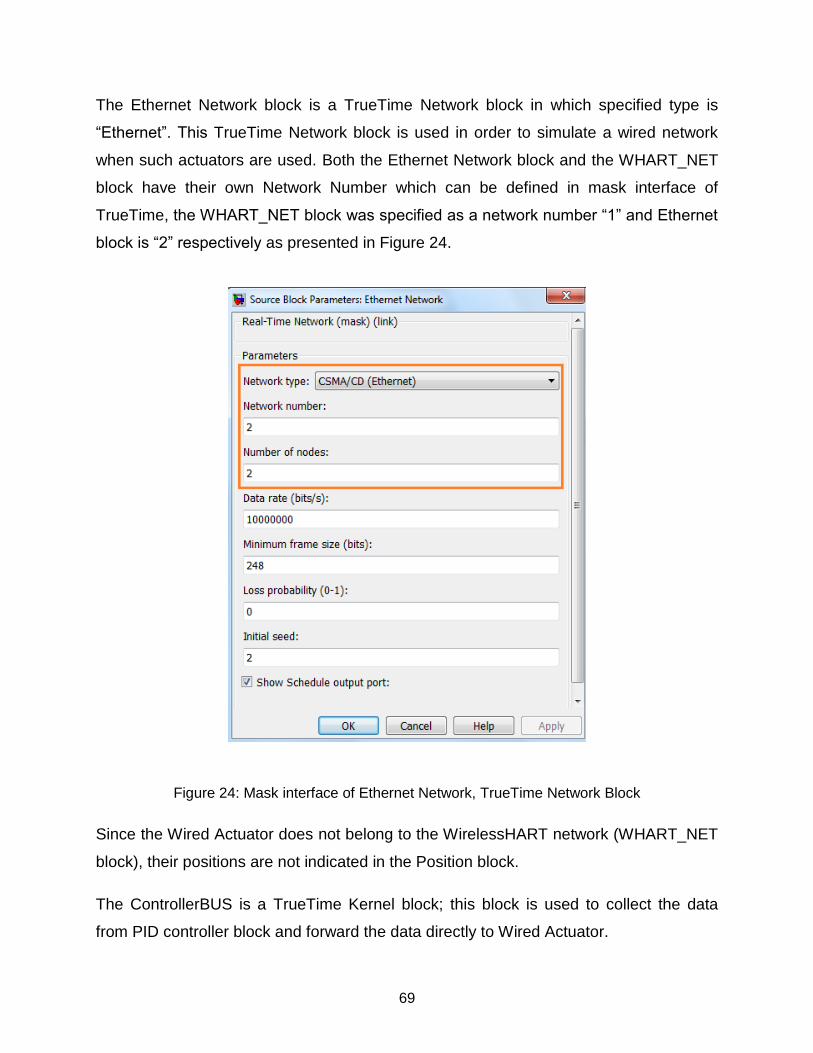
69

The Ethernet Network block is a TrueTime Network block in which specified type is

“Ethernet”. This TrueTime Network block is used in order to simulate a wired network

when such actuators are used. Both the Ethernet Network block and the WHART_NET

block have their own Network Number which can be defined in mask interface of

TrueTime, the WHART_NET block was specified as a network number “1” and Ethernet

block is “2” respectively as presented in Figure 24.

Figure 24: Mask interface of Ethernet Network, TrueTime Network Block

Since the Wired Actuator does not belong to the WirelessHART network (WHART_NET

block), their positions are not indicated in the Position block.

The ControllerBUS is a TrueTime Kernel block; this block is used to collect the data

from PID controller block and forward the data directly to Wired Actuator.

70

Consequent problem/ solution

Since the model has two networks, which are WirelessHART network and Ethernet

network. There was a problem with the controller block. The problem was that in the

model the Controller block could belong to only one network. The question was which

network?

There were two different versions created one where the Controller belonged to the

Ethernet network and one where it belonged to the WirelessHART network. Both

versions were demonstrated to the customer who decided to move on with the version

where the Controller block is part of the WirelessHART network. The reason was that

the Control loops should be scheduled in the WirelessHART schedule.

Figure 25: Simulink Model of two Wireless Sensors, one Wired Actuator and one Wireless

Actuator

According to the Wired Actuator requirement, the customer can generate more

advanced system, where two networks coexist and the system uses both Wired

Actuators and Wireless Actuators.

71

Figure 25 shows the completed simulation model of two Wireless Sensors, one Wired

Actuator and one Wireless Actuator. As mentioned above the number of PID controller

Simulink block will be added in accordance with number of Actuator whether it is the

Wireless Actuator or it is the Wired Actuator. The PID1 connects to Gateway block, this

PID controller responsible to control the Wireless Actuator via Gateway block, while the

PID2 connects to ControllerBus block. The PID2 controller is responsible to control the

Wired Actuator.

6. Evaluation and Results

6.1 Testing the Application

All tests presented here were conducted to ensure that the application still works with

the changes made.

6.1.1 The Reference Model

Referring to Figure 26, the tests all used a simple model of a Servo System as

reference. This model was provided by ABB, to test against. The model was added to

the each Simulation and joined in the Plant Output scopes in order to have a stable

trace on the graphs.

The controller of the reference model is always set with the same parameters as the

networked controller. The step of the reference model was set in a way to minimize the

time delay between the two graphs. The plant (Transfer Fnc) was set to [1] and [3 1 0]

for Numerator coefficients and Denominator coefficients respectively. The RX_DL block

in the reference model was set to 0.0005 s just like the RX delay of each simulation.

72

Figure 26: Servo System Model

6.1.2 Test 1: The performance of the Old WirelessHART Tool and New

WirelessHART Tool

The reason for this test was to see how different the old tool performs compared to the

new tool.

The plant output was recorded in order to see the difference between the two

applications. The PID´s and all settings from the GUI were set identically. However, the

Filter Coefficient (N) in the PID was set in case of the new Tool. Figure 27 and 28 show

the simulation setup model and schedule table of the old version of WirelessHART tool.

73

Figure 27: Old WirelessHART Simulation Setup Model

Figure 28: Schedule table of Old WirelessHART

74

Figure 29: WirelessHART Tool 1.0 (old) against Servo Model

Figure 29 shows the result of the first version of the WirelessHART tool against the

Servo Model. The PID values were tuned in a way that they were supposed to stabilize

plant outputs in the observed time period. The respond time was set to 0.886 sec.

It can be very well seen that the old version of WirelessHART produces a very different

result from the reference model.

The expectation was that the WirelessHART Tool curve should follow the Servo Model’s

curve with a short (approximately 0.03 - 0.04 s) delay with a very slight difference in the

output values. It was also expected that the WirelessHART plant output would stabilize

in the 5 seconds frame what was used for the experiment, but there is no sign of that,

moreover it would be difficult to predict when would it stabilize.

75

Figure 30: New WirelessHART Simulation Setup Model

Figure 31: Schedule table of New WirelessHART

76

Figure 32: WirelessHART Tool 2.0 (new) against Servo Model

Figure 32 shows the result of the new version of the WirelessHART tool against the

Servo Model. The same PID response time was used as in the previous case. The new

version of WirelessHART Tool did perform as predicted before the experiment. The

curves are similar, they both stabilized and the slight difference between the stabilized

lines can be the result of the rounding when the measures are converted to integers and

placed in the network messages.

6.1.3 Test 2: The performance of Wireless Actuator and Wired Actuator

The reason for this test was to see how different does the plant perform with wired and

with wireless actuators.

77

The settings of the networks are the same however in case of the wired actuators, there

was one timeslot less used, to utilize its speed advantage, as shown in Figure 34 and

37.

Figure 33: Wireless Actuator, New WirelessHART Simulation Setup Model

Figure 34: Schedule table of New WirelessHART

78

Figure 35: Wireless Tool 2.0, Wireless Actuator against Servo Model

Figure 35 shows the result of the wireless actuator against servo model in new version

of WirelessHART tool. The PID values were tuned in a way that they were supposed to

stabilize plant outputs in the observed time period. The respond time was set to 0.746

sec. The wireless actuator case did perform as expected closely following the Servo

Model’s performance and stabilizing.

79

Figure 36: New WirelessHART Simulation Setup Model

Figure 37: Schedule table of New WirelessHART

80

Figure 38: WirelessHART tool 2.0, Wired Actuator against Servo Model

Referring to Figure 38, the same PID response time was used as in the previous case.

The Wired Actuators gave the expected results just slightly differing from the results of

the Servo Model.

6.1.4 Test 3: The performance of Multi Channel and Single Channel

The test was conducted in order to assess the advantages of multi channel

communication compared to the single channel communication. As shown in Figure 40

and 42, the scenario was utilizing the shorter schedule in multi channel communication.

In both cases, the same model setup was used, as shown in Figure 39.

81

Figure 39: New WirelessHART Simulation Setup Model

Figure 40: Single channel in Schedule table

82

The result of the experiment was expected in Figure 41. Because of the long

superframe, (0.07 sec) the two control loops were not expected to follow the Servo

Model very closely, but they were expected to produce a similar result to the Servo

Model. It was also predicted that the two control loops results would be very similar

since they used have the same schedule turnaround time (superframe: 0.07 sec).

Figure 41: Result of single channel

83

Figure 42: Multiple channels in Schedule table

As shown in the Figure43, the result of the Multi channel test was completely

unexpected. The expected result was that both control loops would produce very similar

result to the Servo model, but the two control loops just take off without giving a sign to

turn towards the setpoint. The test results show that something was not right with

simultaneous multi channel communication on the WirelessHART network. Since the

actuators did produce outputs, the only explanation is that the messages did not arrive

from the sensors after they were sent. The reason is that TrueTime does not support

multiple frequency (channels) communication.

Figure 43: Result of Multiple channels

84

7. Discussion of Results

Test 1: The improvement of the WirelessHART Tool performance

When comparing the performance of the old tool and the new tool, the expectations

were that the plant output using the new tool would be more similar to the plant output

of the Servo model than when using the old tool.

The expectations were right the new Tool was way closer when comparing the results.

The reasons for the performance difference are most likely to be the updates to the

controller (both on the GUI and in the Simulation Model), since there were no changes

made to the network or TrueTime.

Test 2: The performance of Wireless Actuator and Wired Actuator

The expectations in the second test were that the wired actuators would outperform (get

closer) results to the Servo Model than the wireless actuators.

The forecast for test was right; the simulation using wired actuators did give a plant

output closer to the Servo Model than the simulation using the wireless actuators. The

reason is for the result is that the schedule turnaround time (superframe length) is

shorter when using wired actuators.

Test 3: The performance of Multi Channel and Single Channel

The assumption before the test was that the plant output of the simulation utilizing the

multi-channel functionality would get closer to the plant output of the Servo Model. The

reason for making this assumption is that shorter superframes could be used and were

used for the simulation with the multi-channel functionality.

The assumptions were wrong. The messages, which were sent in the first timeslot and

contained the sensor values, did not arrive on the receiving node. After a short

investigation, it was found that the multi-channel functionality was not implemented in

TrueTime for WirelessHART.

85

8. Conclusion and Future work

The goal of this thesis was to evaluate the existing WirelessHART Tool, add new

functionality without affecting already existing features and attempt to improve where

problems are found.

Before the implementation started, the authors had to familiarize themselves with topics

such as network theory, WirelessHART standard etc. and get to know the existing

application structure of WirelessHART Tool in order to be able to map the new

functionality.

There were many questions unanswered after the conducting research. In order to be

able to proceed with the implementation, the unanswered questions were discussed

with the customer and the appropriate solution was chosen. Each specific solution was

evaluated and developed. In order to verify the correctness of the whole application, a

few test specifications were created, used to assess the application and the results

along with the specifications were demonstrated to the customer.

Some of these tests can be found in this paper. The results of the test comparing the

old application to the new application have full-filled the expectations.

The comparison of the wired and wireless actuators has given the expected results as

well.

The test, comparing the multi-channel and single channel communication gave a

surprising result. The multi-channel communication turned out not to be working at all.

After a short investigation, it turned out that the problem was in the TrueTime

implementation of WirelessHART. The problem was taken into discussion with the

customer, who decided that there was not to correct the functionality in TrueTime.

Considering the documentation, the missing parts about the application structure, and

functionality were added.

There are some suggestions, which should get priority when considering future work, on

WirelessHART Tool.

86

First of all, there is possibility to implement object-oriented design in MATLAB. If the tool

was implemented that way, it would be easier to extend, maintain, and respond faster.

Another suggestion is to reorganize the old code. Use different folders for files and

move out the body of the callbacks from the GUI’s callback file into different files.

The application needs additional testing of all its functionality and the simulation results

need to be compared to some real life scenarios to see how reliable the tool is.

TrueTime has to be modified in order to support multi-channel communication in

WirelessHART. Since the feature in WirelessHART Tool is already implemented, there

is no reason why it could not be used as soon as TrueTime is modified.

Otherwise, WirelessHART Tool proved to be a useful application with plenty of potential

for other functionality such as, creating interface for testing automatic scheduler

algorithms, an interface to allow easy replacement of the controller by external

controllers in order to test their performance etc.

87

References

[1] Carlos A. Smith, Automated Continuous Process Control, A Wiley-Interscience

Publication, 2002

[2] M. Jouaneh, Fundamentals of Mechatronics Si Edition, Cengage Learning, 2013

[3] S.C. Goyal, U.A. Bakshi, Feedback Control Systems, Technical Publications

Pune, 2008

[4] Andrew Hunt, David Thomas, The Pragmatic Programmer from journeyman to

master, Addison Wesley Longman Inc, 2000

[5] Jingyu Liu, Yanjun Fang, Dahai Zhang, “PROFIBUS-DP and HART Protocol

Conversion and the Gateway Development”, In proceeding of Second IEEE

conference on Industrial Electronics and Applications, 2007

[6] Nitaigour P. Mahalik, Fieldbus Technology: Industrial Network Standards for

Real-Time Distributed Control, Springer, 2003

[7] HART Communication Protocol - HART Specifications,

http://www.hartcomm.org/protocol/about/aboutprotocol_specs.html, (visited 24,

July, 2012)

[8] HART communication foundation - TDMA Data Link Layer - HCF SPEC _ 075

Revision 1.0, 2007

[9] HART Communication Protocol - WirelessHART Components,

http://www.hartcomm.org/protocol/wihart/wireless_components.html, (visited 24,

July, 2012)

[10] Anton Cervin, Dan Henriksson, Martin Ohlin, TrueTime 2.0 beta –

Reference Manual, Lund University, 2010

[11] Sara Z. Afshar, Mohammand Ashjaei, WirelessHART Simulator – A GUI

for simulation of WirelessHART network in TrueTime toolbox – Technical Report,

ABB research cooperate, 2011

88

[12] Write Code for Callbacks:: Code a Programmatic GUI (MATLAB),

MathWorks, http://www.mathworks.se/help/techdoc/creating_guis/f16-

999606.html#f16-999626, (visited 24, July, 2012)

[13] Sara Z. Afshar, Mohammand Ashjaei, WirelessHART Simulator – A GUI

for simulation of WirelessHART network in TrueTime toolbox – User Manual,

ABB research cooperate, 2011

[14] Donald R. Gillum, Industrial Pressure, Level, and Density Measurement

Second Edition, International Society of Automation, 1995

[15] Raimond Pigan, Mark Metter, Automating with PROFINET, Wiley-VCH,

2008

[16] Diane Barrett, Todd King, Computer Networking Illuminated, Jones and

Bartlett Publishers, 2005

[17] A. Willig, K. Matheus, A. Wolisz , “Wireless Technology in Industrial

Networks”, In IEEE Software, volume 93, pages 1130-1151, 2005

[18] Leena G. Jeevana, Vini Malikb, “A Wavelet Based Multi-Resolution

Controller”, In Journal of Emerging Trends in Computing and Information

Sciences, volume 2, 2011

[19] Shahin Farahani, Zigbee Wireless Networks and Transceivers, Newnes,

2003

[20] Len Bass, Paul Clements, Rick Kazman, Architecture in Practice Second

Edition, Addison Wesley, 2003

[21] Nick Rozanski, Eoin Woods, Software Systems Architecture: Working with

Stakeholders Using Viewpoints and Perspective, Addison Wesley, 2011

[22] Tomas Lennvall, Stefan Svensson, Fredrik Hekland, “A Comparison of

WirelessHART and Zigbee for Industrial Applications”, In IEEE International

Workshop on Factory Communication System, 2008

[23] Deji Chen, Mark Nixon, Aloysius Mok, WirelessHART Real-Time Mesh

Network for Industrial Automation, Springer, 2010

[24] Jianping Song, Song Han, Al Mok, Deji Chen, Mike Lucas, Mark Nixon,

Wally Pratt, “WirelessHART: Applying Wireless Technology in Real-Time

89

Industrial Process Control”, In IEEE Real-Time and Embedded Technology and

Applications Symposium, pages 377 – 386, 2008

[25] Osama Khader, Andreas Willing, Adam Wolisz, Implementation and

Evaluation of Communication Tables and Link Scheduling for WirelessHART

Devices, TKN Technical Reports Series, Technical University Berlin, 2011

[26] Mauro De Biasi, Carlo Snickars, Krister Landernäs, Alf Isaksson,

“Simulation of Process Control with WirelessHART Networks Subject to Clock

Drift”, In IEEE International Computer Software and Applications Conference,

pages 1355- 1360, 2008

[27] Norihiko Morinaga, Ryuji Kohno, Seiichi Sampei, Wireless Communication

Technologies: New Multimedia Systems, Springer, 2002

[28] Software technologies group, Zigbee versus other wireless networking

standards, http://www.stg.com/wireless/Zigbee_comp.html, (visited 24, July,

2012)

[29] Hongyi Wu, Yi Pan, Medium Access Control in Wireless Networks, Nova

Science Publishers, 2008

[30] Changjiang Li, Yufen Wang, Xiaojuan Guo, “The Application Research of

Wireless Sensor Network Based on Zigbee”, In IEEE International Conference on

MultiMedia and Information Technology, 2010

[31] Quick Start (MATLAB), MathWorks,

http://www.mathworks.se/help/techdoc/learn_matlab/bta3so7.html, (visited 24,

July, 2012)

[32] Simulink Documentation, MathWorks,

http://www.mathworks.se/help/toolbox/simulink/?s_iid=SL2012_bb_doc, (visited

27, July, 2012)

[33] What is an S-Function? - Overview of S-Function (Simulink), MathWorks,

http://www.mathworks.se/help/toolbox/simulink/sfg/f6-151.html, (visited 27, July,

2012)

[34] M. Urban, M. Blaho, J. Murgas, M. Foltin, Simulation of Networked Control

Systems via TrueTime, Institute of Control and Industrial informatics - Slovak

University of Technology, 2008

90

[35] Dan Henriksson, Anton Cervin, Karl-Erik Årzén, TRUETIME: Real-time

Control System Simulation with MATLAB/Simulink, Automatic Control – Lund

Institute of Technology, 2007

[36] Zigbee Specifications, http://zigbee.org/Specifications.aspx, (visited 28,

July, 2012)