Master Thesis 2018-2019

Master Thesis

2018-2019

GREENHOME: HOUSEHOLD ENERGY CONSUMPTION & CO2 FOOTPRINT METERING ENVIRONMENT

KHALIL MAYSAA

Master in Electrical Engineering for Smart Grids and

Buildings

Laboratoire d’Informatique de Grenoble – LIG

&

Laboratoire de Génie Électrique de Grenoble - G2Elab

Supervised by

Mme. Genoveva VARGAS-SOLAR, Senior Scientist, CNRS, LIG

M. Javier ESPINOSA, Scientist, University of Technology of Delft

M. Raphael CAIRE, Professor, Grenoble INP, G2ELAB

Non-Confidential

Application to decision support for electricity sector | Maysaa Khalil

pg. 2


pg. 3

STATEMENT ON ACADEMIC INTEGRITY

I hereby declare and confirm with my signature that the master thesis / dissertation is exclusively the result of my own autonomous work based on

my research and literature published, which is seen in the notes and bibliography used.

I also declare that no part of the paper submitted has been made in an inappropriate way, whether by plagiarizing or infringing on any third

person's copyright.

Grenoble, 06/23/2019

Maysaa KHALIL


pg. 4

“It is difficult to make predictions, especially about the future” NEILS BOHR, Danish physicist


pg. 5


pg. 6

Abstract

The recent increase in smart meters in the residential sector leads to large available dataset. Reducing energy consumption is a challenge that requires best utilize of the available data. Predicting energy consumption should help customers increase efficiency and reduce carbon footprint. However, this is not a trivial task as consumption on low voltage has an irregular behavior. This report presents the GREENHOME environment, a toolkit that provides several data analytics tools for metering household energy consumption and CO2 footprint under different perspectives. Through different statistics and data mining algorithms, the environment enables a multi-perspective analysis of household energy consumption and CO2 footprint using and combining different variables. The problem of load forecast is addressed using two machine-learning methods, the autoregressive integrated moving average model (ARIMA) and autoregressive with exogenous terms model (ARX). For a case study in a house in Picardie, hourly energy consumption data were available for the year of 2018. Results indicate that the ARX model generates a better residential mean square error RMSE than the ARIMA model. It was shown that by adding exogenous variables the performance of the model increases. Both models show a better performance than the naïve forecast model- persistence method.


pg. 7

RÉSUMÉ

L'augmentation récente du nombre de "capteurs intelligents" dans le secteur résidentiel donne accès à un vaste ensemble de données disponibles. Réduire la consommation d'énergie est un défi qui nécessite une utilisation optimale de ces données. La prévision de la consommation d’énergie devrait aider les clients à accroître leur efficacité et à réduire leur empreinte carbone, mais cette tâche n’est pas anodine, car la consommation énergétique à basse tension est de forme irrégulière. Ce rapport présente l’environnement GREENHOME, une boîte à outils proposant plusieurs outils d’analyse de données permettant de mesurer la consommation d’énergie et l’empreinte CO2 des ménages. A l'aide de différentes méthodes statistiques et plusieurs algorithmes d'exploration de données, l'environnement permet une analyse multi-perspective de la consommation d'énergie et de l'empreinte CO2 des ménages en utilisant et en combinant différentes variables. Le problème de "load forecasting" est traité à l'aide de deux méthodes « machine learning », le modèle ARIMA qui est autorégressif et intègre une moyenne mobile, et le modèle ARX, modèle autorégressif avec des termes exogènes. Une étude de cas a été faite sur une maison située en Picardie. Les données de consommation d'énergie horaire étaient disponibles pour l'année 2018. Les résultats indiquent que le modèle ARX génère un meilleur RMSE par rapport au modèle ARIMA. Il a été montré qu'en ajoutant des variables exogènes, la performance du modèle augmentait. Les deux modèles affichent de meilleures performances comparées à la méthode de prévision naïve du modèle de persistance.


pg. 8

Contents CHAPTER 1 INTRODUCTION ................................................................................................................... 12

1.1 CONTEXT AND MOTIVATION............................................................................................................... 12 1.1.1 Smart Metering Infrastructure ............................................................................................... 12 1.1.2 Smart Grid Analytics ............................................................................................................... 13

1.2 ANALYZING AND PREDICTING BUILDINGS ENERGY CONSUMPTION ............................................................. 14 1.3 OBJECTIVE AND MAIN CONTRIBUTION ................................................................................................. 14 1.4 ORGANIZATION OF THE DOCUMENT..................................................................................................... 14

CHAPTER 2 BACKGROUND AND STATE OF THE ART ............................................................................... 15

2.1 BIG DATA PROCESSING FOR SMART GRID ............................................................................................... 15 Smart Metering Environment ............................................................................................. 15

2.1.2 Smart Metering Data Analytics .......................................................................................... 15 2.1.3 Power Load Analysis ........................................................................................................... 16 2.1.4 Smart Grid Big Data Analytics Architectures ...................................................................... 17

2.2 FORECASTING ENERGY CONSUMPTION ................................................................................................. 19 2.2.1 Forecasting Models ............................................................................................................ 19 2.2.2 Forecasting Pipeline ........................................................................................................... 19

2.3 SMART METERING SYSTEMS AND APPLICATIONS .................................................................................... 21 2.4 DISCUSSION .................................................................................................................................... 22

CHAPTER 3 GREENHOME SMART METERING ENVIRONMENT ................................................................ 23

3.1 SMART ENERGY AND CO2 FOOTPRINT METERING ENVIRONMENT ............................................................. 23 3.1.1 Sensing, Fusion and Storage Layers .................................................................................... 23 3.1.2 Analytics and Prediction Layer ........................................................................................... 24

3.2 EXPERIMENT SETTING ....................................................................................................................... 24 3.2.1 Implementation Environment ................................................................................................. 25 3.2.2 Methodology .......................................................................................................................... 25

3.3 DATA COLLECTIONS PREPARATION ...................................................................................................... 26 3.3.1 Quantitative Profile of Data Collections ............................................................................. 26 3.3.2 Extreme Value Analysis ...................................................................................................... 27 3.3.3 Proximity Method ............................................................................................................... 29 3.3.4 Interquartile Range Method ............................................................................................... 30 3.3.5 Comparison and Bad Data Replacement ............................................................................ 30

3.4 COMPUTING HOUSEHOLD ENERGY CONSUMPTION AND CO2 FOOTPRINT MODELS ....................................... 30 3.4.1 Sensitivity Analysis Using the Morris Model ....................................................................... 30 3.4.2 Mathematical Estimation of the CO2 Footprint .................................................................. 31

3.5 PREDICTING HOUSEHOLD ENERGY CONSUMPTION AND CO2 FOOTPRINT.................................................... 32 3.5.1 Naïve Forest Persistence Model ......................................................................................... 32 3.5.2 ARIMA Model ..................................................................................................................... 33 3.5.3 ARX Model .......................................................................................................................... 36

3.6 DISCUSSING RESULTS ........................................................................................................................ 37

CHAPTER 4 CONCLUSION AND FUTURE WORK ................................................................................ 38

4.1 MAIN RESULTS AND CONTRIBUTION .................................................................................................... 38 4.2 PERSPECTIVES.................................................................................................................................. 38


pg. 9

BIBLIOGRAPHY ....................................................................................................................................... 39

APPENDIX A BAD DATA DETECTION METHODS ...................................................................................... 43

APPENDIX B PSEUDOCODES FOR PREDICTING MODELS USED ................................................................ 45

PERSISTENCE MODEL AND COMPLEXITY MEASURES ............................................................................................. 45 ARIMA MODEL AND COMPLEXITY MEASURES ................................................................................................... 46

APPENDIX C PYTHON LIBRARIES USED ................................................................................................... 48

APPENDIX D SENSITIVITY ANALYSIS AND CORRELATION STUDY ............................................................ 49

MORRIS METHOD ......................................................................................................................................... 49 AUTOCORRELATION PLOTS .............................................................................................................................. 49

APPENDIX E SMART METERING APPLICATIONS & ENVIRONMENTS ....................................................... 51

Social Smart Metering ......................................................................................................................... 51 Triple-A Environment ........................................................................................................................... 51 NetatMo Application ........................................................................................................................... 52 TOON® Application ............................................................................................................................. 52 Comparison .......................................................................................................................................... 52


pg. 10

Table of tables Table 1 Comparison between Data warehouse, Hadoop and stream computing ........................ 18

Table 2 Quick Statistical Information on the hourly energy consumption ................................... 26

Table 3 Carbon Emission Factor from Triple-A project ................................................................. 31

Table 4 Brief statistics for residual error ....................................................................................... 35

Table 5 Summary of existing environments .................................................................................. 54


pg. 11

Table of figures Figure 1 Challenges related to smart grid analytics ...................................................................... 13

Figure 2 Number of publications indexed by WoS ........................................................................ 14

Figure 3 Top Analytics Initiatives ................................................................................................... 16

Figure 4 Purpose of different types of analytics ........................................................................... 16

Figure 5 Smart metering architecture deployed on the cloud ...................................................... 18

Figure 6 Smart Energy and CO2 footprint Metering Environment Architecture .......................... 23

Figure 7 Energy consumption before sampling ............................................................................. 27

Figure 8 Daily Energy Consumption in 2018.................................................................................. 27

Figure 9 Energy Consumption per hour grouped by month ......................................................... 28

Figure 10 Scatter plot for energy consumption per hour grouped by months ............................. 28

Figure 11 Daily energy consumption over one year ...................................................................... 28

Figure 12 Boxplot for daily energy consumption grouped by months .......................................... 29

Figure 13 Boxplot for hourly energy consumption grouped by month ........................................ 29

Figure 14 K-means clustering for hourly electric consumption with k=4,12................................. 29

Figure 15 Impact of different input variables on the energy consumption .................................. 31

Figure 16 Carbon footprint of hourly energy consumption .......................................................... 32

Figure 17 Persistence forecast model ........................................................................................... 33

Figure 18 Non-stationary plot of energy consumption ................................................................. 34

Figure 19 Autocorrelation plot (left) & partial autocorrelation plot (right) .................................. 34

Figure 20 Distribution of residual error ......................................................................................... 35

Figure 21 ARIMA Forecast Model plot .......................................................................................... 36

Figure 22 ARX Forecast Model plot ............................................................................................... 37

Figure 23 Box-and whisker plot for outlier detection ................................................................... 43

Figure 24 Anomaly detection with proximity method .................................................................. 43

Figure 25 Outlier detection in projection method ........................................................................ 44

Figure 26 Morris Method Example ................................................................................................ 49

Figure 27 Autocorrelation Plot Example ....................................................................................... 50

https://d.docs.live.net/1a8854299f00f8b7/Report2.docx#_Toc12274652








pg. 12

Chapter 1 INTRODUCTION My internship was done at Laboratory of Informatics of Grenoble (LIG1) in the Heterogeneous and Adaptive Distributed Data management Systems team (HADAS). The HADAS research project addresses new challenges raised by continuous generation of huge, distributed, and heterogeneous data. These challenges concern collection/harvesting, integration, lookup and querying, filtering and indexing.

1.1 Context and Motivation

Global warming and its impending follow-ups have become a major global issue. Scientists and governments have agreed that cleaner and sustainable solutions can help in reducing the impact of this phenomenon. Thus, governments have implemented measures to reduce greenhouse gases emissions, the major catalyst for global warming [1][2]. Studies [3][4] have agreed that the energy sector, specifically the electric one has a vital impact on emissions and can be regulated by public policies to reduce greenhouse gases emissions.

According to EU statistics [5], buildings represent 40% of all energy consumption and 36% of CO2

emissions in Europe due to the age of buildings in Europe. Studies[6] show that if the current energy consumption pattern persists, the world energy consumption will increase more than 50% before 2030. The concept of smart building has been introduced to address problems implied by this observation. The principle is to integrate “datification2” into buildings to optimize their usage in terms of comfort and energy. A smart building uses sensors and software for automating some processes like control lighting [7], climate [8], entertainment systems, and appliances [9]. It may include home security [10] such as access control and alarm systems and occupancy measures [11]. This leads to the need of data to be collected, processed and analyzed to enhance the efficiency of the energy consumption and of the energy grid [12]. Therefore, different models have been proposed to measure and predict energy consumption and CO2 emissions in buildings.

1.1.1 Smart Metering Infrastructure

The integration of smart measuring devices in a household via Internet of things (IoT) allows collecting information used for generating beneficial insights to increase energy efficiency in households and turn them into smart ones[13]. The main target is to achieve a smart management of electric energy. The energy consumption environment is an advanced metering infrastructure (AMI) that measures, collects, analyzes consumption, and communicates with metering devices according to a schedule or on request [14][15].

Smart metering data can benefit the players of a smart metering community (DSO3, retailer, consumer, aggregator, and data service provider) [12] to: (i) Reduce energy consumption and decrease electrical bills through load forecasting (consumers & aggregators). (ii) Increase competitiveness and profits in the retail markets through load forecasting, price design, abnormal event detection and services provided to consumers. (iii) Distribution and outage management in network topology (DSO). (iv) Load analysis forecast and management to support players decision making using analytics (predictive, descriptive, and prescriptive). Techniques used for forecasting

1 http://liglab.imag.fr 2 Modern trend that turns many daily life aspects into data. It has been attached to different analysis of representations of daily life events captured by data, https://en.wikipedia.org/wiki/Datafication 3 DSO is the distribution system operator responsible for the transmission of electricity on high voltage, medium voltage and low voltage distribution system with a view to its delivery to the customer, without including supply to the customer.


pg. 13

energy consumption time series data and outlier detection are still open. This work addresses this challenge.

1.1.2 Smart Grid Analytics

To gauge how far utilities have come, the Utility Analytics Institute (UAI) fielded the “State of Smart Grid Analytics Survey” in January 2017 [16].The surveyed respondents’ job vary from chief operating officers to engineers to analysts and they represent many different business functions. One survey, done on 75 respondents, addressed the challenges related to the integration of smart grid analytics shown in Figure 1.

Figure 1 Challenges related to smart grid analytics

Data availability/access seems to be the most popular challenge in the utilities followed directly by both the skilled staff and lack of centralized location for data storage. Clearly, the main challenge nowadays, estimated by 60% of whole challenges is the current state of data itself and the lack of people who knows what to do with it. Another thing to spot light on is that the budget is not the number one challenge in the grid analytics having a percentage of 13%.

In order to have a global view on the existing research related to data analytics contributing to smart grid, a bibliometric analysis was done on 31 December 2017 using Web of Science4 (WoS), which is an online citation indexing service that provides a comprehensive search. The query was:

TS=((“smart meter” OR “consumption” OR “demand” OR “load”) AND “data” AND (“household” OR “resident” OR

“residential” OR “building” OR “industrial” OR “individual” OR “customer” OR “consumer”) AND (“energy theft” OR

“demand response” OR “clustering” OR “forecasting” OR “profiling” OR “classification” OR “abnormal” OR “anomaly”)

AND (“smart grid” OR “power system”)) (Yi Wang, Qixin Chen, Tao Hong, Chongqing Kang)

Figure 2 Number of publications indexed by WoS(left) shows the evolution in the number of publications throughout the years since 2011. In total, only 2 hundred publications were found in WoS until that time. Note that before 2011, no publications were done on the topic discussed relating data analytics to the smart grid. This is mainly due to the fact that before 2000, the term “smart grid” was not well known, and it will take about 10 years to collect data for analysis after the installation of the smart meters. Figure 2 Number of publications indexed by WoS (right) lists the journals in increasing order by the number of papers, which were published since 2010 according to WoS. IEEE Transactions on Smart Grid, the youngest journal between the listed ones, has published 28 papers since its launching in 2012.

4 webofknowledge.com


pg. 14

Figure 2 Number of publications indexed by WoS

1.2 Analyzing and Predicting Buildings Energy Consumption

Discovering, analyzing and predicting energy consumption in buildings is an emerging research area. Most energy load forecast models have addressed high voltage level. Developing a highly accurate forecast is nontrivial at lower levels [12]. However, with data provided by smart meters at low voltage level, opportunities are open to improve prediction. Methods have been proposed to predict energy consumption at the lower level. Some do not consider smart meter data, like [17] that proposes a two-stage long-term retail load forecast model considering the residential customer’s attrition. Others do consider smart meter data to forecast micro-grid settings[18], to learn spatial information shared among interconnected customers and to address the over-fitting challenges[19], to predict buildings time series data [20].

1.3 Objective and Main Contribution

The objective of this work is to predict energy consumption in a household and calculate the CO2 footprint produced due to the energy consumed. Therefore, our work compares two autoregression methods (autoregressive integrated moving average model -ARIMA- and autoregressive with exogenous terms model -ARX) used to predict electric consumption time series data.

The main contribution is GREENHOME smart metering environment for energy consumption and carbon footprint inside buildings. The environment has been tested through a case study that analyses energy consumption inside a household in Picardie. It estimates the carbon footprint resulted from the consumed energy, compares between a naïve forecast model, an ARIMA model and an ARX model for best designing an energy forecast model.

1.4 Organization of the Document

The remainder of this document is organized as follows:

Chapter 2 Background and State of the Artintroduces the background of the work related to Big Data fundamental characteristics described in the V’s model. It enumerates the aspects in which Big Data analytics can contribute to Smart Grid and particularly to energy consumption studies. Finally, the chapter describes, smart metering environments that estimate energy consumption.

Chapter 3 GREENHOME SMART METERING ENVIRONMENT introduces GREENHOME the proposed environment to build a multi-perspective analysis of household energy consumption and CO2

footprint combining different variables. The chapter describes its implementation and discusses analytics results with respect to a use case.

Chapter 4 Conclusion and Future Work concludes the work done after spotting light on the main results and the contributions to the project. It also enumerates research perspectives.


pg. 15

Chapter 2 Background and State of the Art This chapter introduces the background concepts necessary to understand our work and the state of art. The chapter is organized as follows. Section 2.1 enumerates the aspects in which Big data analytics can contribute to Smart Grid. Section 2.2 describes, and analyses approaches used for forecasting energy consumption. Section 2.3 presents the different smart metering systems and applications. Section 2.4 discusses the state of art and open issues.

2.1 Big Data processing for Smart Grid

Big data proposes strategies to analyze, extract information, and deal with data sets that are too large or complex for traditional data-processing systems[21] [22]. There is a consensus about its characteristics described by the V’s model [22]: (i) volume referring to the size of the data collections produced, processed and stored; (ii) velocity, referring to the data production rate; (iii) variety describing the heterogeneity of models and data formats; (iv) veracity referring to data accuracy, truthfulness, and meaningfulness; (v) value referring to the economic and non-economic capital that can potentially generate data. Other V’s are also considered like validity[22] to refer to the period during which data are representative and valid for a given use and visibility[22] determining the point of view from which data are collected and processed.

Analyzed and extracted big data can be collected using different smart meters installed in buildings to gather information regarding the energy and gas consumption, meteorological measures and residents’ behavior. The ability to extract useful insights using big data processing can improve the efficiency of the smart grid, decrease consumption and maintain a production-consumption real time balance.

Smart Metering Environment

Metering is the process of measuring physical variables like gas and electric consumption, temperature, humidity, occupancy, etc. A metering infrastructure is a system that measures, collects, and analyzes data collected by meters. Internet of Things (IoT) is an infrastructure of interrelated devices, mechanical and digital machines, and objects. Applied to electric utilities in buildings promotes the implementation of a ‘Smart Building’.

A smart meter is an electronic device that records electric energy consumption and communicates data to the electricity supplier for monitoring and billing [23]. The high frequency of data readings opens new possibilities for understanding the electricity demand network [24]. By providing real time data, a smart meter allows utility providers to optimize energy distribution while allowing consumers make smarter decision about their energy consumption and associated carbon impact [25].

2.1.2 Smart Metering Data Analytics

The survey reported in [26] queried people on top analytics initiatives. It shows that system modeling, asset optimization and outage management are the drivers in utility operational expenditures (see Figure 3). The conditions in which the utility industry operates, and its asset-intensive nature explains that the system modeling is on the top of the list.


pg. 16

Figure 3 Top Analytics Initiatives

To support the business of players, analytics has to be done and its type varies along a continuum [26] that includes (see Figure 4): (i) Descriptive analysis consisting of data visualization, data mining and aggregation reports targeting the understanding of the data stemming from consumption sensing to decide how to process it. (ii) Diagnostic analytics targets the identification of the cause of given events. (iii) Predictive analytics targets the ability to make probabilistic predictions. (iv) Prescriptive analytics utilizes techniques like simulation and decision support to find the optimal strategies that can mitigate future risks.

Figure 4 Purpose of different types of analytics

2.1.3 Power Load Analysis

Load analysis is a power analysis performed on the distribution system to ensure balancing and no overloading in any place on the grid. Load analysis results can be further used for load forecast and demand response programs. In this section, load analysis is defined through two points:

Anomaly detection 5 [12] addresses the identification of strange items, events or observations, which raise suspicion and that can be considered as bad data. Bad data can refer to missing values, unusual patterns caused by unplanned events like an abnormal stop of the smart meter, restart phenomenon that resulted in failure during data collection and communication.

Load profiling is used to determine basic electricity consumption patterns of different costumers’ groups by classifying consumers’ load curves according to their energy consumption behavior. There are two ways to perform load profiling: (i) Direct clustering-based approach with different classification techniques used like K-means[20], hierarchical clustering[27], and self-organizing

5 Anomaly detection refers to the identification of rare observations that raises suspicious after being significantly different form the other observations

0% 5% 10% 15% 20% 25% 30% 35% 40%

System modeling

Asset optimization

Outage management

Distributed energy resource management

Grid optimization

Transmission and distribution asset management

Analytics for real-time management

Advanced distribution management

Power quality optimization

Other

Substation equipment management

Transformer management

What are the top analytics projects your group is currently working on? (n = 75)


pg. 17

map (SOM)[28]. (ii) Indirect clustering includes dimensionality reduction, load characteristics and uncertainty-based methods depending on the features extracted before clustering.

Note that most clustering techniques use historical data, which requires the emergence of new techniques to deal with the huge amount of streaming data gathered by smart meters.

Load Forecasting accuracy has its great weight on the operational loading of a utility company as well as the reduction in energy consumptions for end users. Smart meters data contribute to the implementation of load management in two aspects:

- Customer Characterization: The electricity consumption profile is related to the customer’s sociodemographic status. This allows the classification of customers. Therefore, the point is to recognize sociodemographic information about customers from load profiles and predict the loads according to their sociodemographic classification. Different techniques including fast Fourier transformation, sparse coding, and clustering where used to classify customers. In addition, data like location, floor area, age of consumers, and number of appliances may help in the classification.

- Demand response implementation (DR): Briefly, DR is a change in the normal consumption electric usage by end users. This change is due to a response to changes in the price over time or to incentive payments[29]. DR has played a vital role in balancing the supply and demand for electrical load[30]. Bill rebates, redeemable vouchers, discounts are some incentive payments derived from DR programs. DR programs may lead to success only if these two factors are achieved: (i) how to operate DR resources which is mainly related to customers, energy market, devices and utility company; and (ii) how to measure DR performance. Yet, traditional baseline estimation lacks the ability to characterize uncertainties due to their deterministic modeling. This deficiency often results in erroneous system operations and miscalculated payments that discourage participating customers[31].

2.1.4 Smart Grid Big Data Analytics Architectures

The main objective of big data analytics is to explore and process data, and transform it into meaningful information such as patterns of operation, alarm trends, fault detection, and control commands [26]. It uses techniques proposed in different domains like data mining, statistical analysis, machine learning and artificial intelligence (AI). Smart Grid Analytics uses data science processes for combining different solutions including Data warehouses DWH, large scale data processing frameworks (e.g., Hadoop) and real time processing (stream computing) [32]. - Data warehouses (DWH) are used for storage. - Apache Hadoop is an open source software library, a framework that allows for the parallel

processing of large data sets across clusters of commodity hardware using simple programming models.

- Stream computing tools monitor millions of events in a specific time window to react proactively, they are behavior-based architecture where events are analyzed in real time and action performed and then stored in databases for further analytics.

Table 1 Comparison between Data warehouse, Hadoop and stream computingshows a comparison among the three software components. The type of data stored can be structured or not. Different purposes arise from this storage including reporting, long run computation and real time analysis. The age of data range between old and new. The size of data varies as well depending on the element, it varies between kilo bytes and terra bytes. The speed of processing varies depending on the need of the analysis, report or computation. It varies between Mbps to


pg. 18

Peta bytes. The cost varies as well depending on the nature of computation. Data volume varies among different components. Some components do not take into consideration data velocity and variety.

Characteristics Data warehouse Hadoop Stream Computing

Type of data stored Structured Structured and

Unstructured

No storage

Storage purpose Reporting and dashboard Long run computation Real time analysis

Age of data Old Past Current/new data

Size of data Terra/Peta bytes Giga bytes Kilo bytes

Speed of processing Peta bytes/ day Kbps Mbps

Implementation cost High Medium Low

Volume High High Low

Velocity Nil Nil High

Variety Nil High High

Table 1 Comparison between Data warehouse, Hadoop and stream computing

The smart metering components can be deployed in the cloud [33] using multiple backend services that communicate with the outside using three interfaces (see Figure 5 Smart metering architecture deployed on the cloud).

- Cloud gateway communicates with the sensors. It ingests device telemetry and ensures that the target devices reliably receive control messages.

- Web Application Server is responsible for house residents and administrators’ interface. It provides a user interface necessary for data visualization and device management and monitoring. It is also responsible for securing these interfaces.

- Protocol Bridge provides the connection between the platform and an external platform. It translates between common application protocol and the protocol used by external system.

Mesh networks (e.g. Zigbee, Wi-SUN)

Cellular Networks (e.g. NB-IoT,

LTE Cat-M1, GRPS)

Sub-GHz (169-925 MHz)

Networks (e.g., LoRaWAN, Sigfox)Wi-Fi

Cloud Gateway

Device

Provisioning,

Authentication, and

Management

Offline Data

AnalysisData Storage

Stream

Analytics

Pro

toco

l B

rid

ge Web Application Server

UtilityUserExternal

Platform

Wi-FiSmart Sensor

Protocol-Specific Field Gateway

(Network Base Station/Coordinator)

Cellular Bus Station

External High

Bandwidth link

Internal High

Bandwidth link

External Low

Bandwidth link

Figure 5 Smart metering architecture deployed on the cloud


pg. 19

2.2 Forecasting Energy Consumption

Analyzing time-oriented data and forecasting values using time series6 are important problems that analysts face in the field of energy consumption [34]. The focus is on short- to medium-term forecasting where statistical methods are useful. Short-term predictions provide forecasting over a period of days, weeks, or months to the future. Short-term forecast is commonly based on identifying, modelling and interpolating patterns and insights launched by historical data. The reason why forecasting in the electric consumption time series is important is that predictions are critical for various decision-making tasks including estimating carbon footprint, reducing energy consumption, etc. The forecast here is considered as a quantitative forecast, where the model uses historical data, it formally summarizes patterns in data and statistically outcome a relationship between the previous records and the estimated ones.

2.2.1 Forecasting Models

There are mainly three groups of forecasting models including engineering, statistical and artificial intelligence models. A review on prediction methods can be found in [13] and [35]. Engineering methods, which are detailed comprehensive methods, use the structural characteristics of the building in the form of physical principles and thermodynamic equations as well as environmental information including climate conditions and occupants’ activities. However, these methods need fine grained details about the structure and the thermal characteristics of the building that unfortunately are not always available [36]. Statistical methods use historical data to correlate between instance consumption and previous consumptions as well as most influencer variables. Consequently, the quality and quantity of historical data possess a crucial role on the developing of the model. Regression models, conditional demand analysis (CDA), auto regressive moving average (ARMA), auto regressive integrated moving average (ARIMA) and Gaussian mixture models (GMM) are some examples of statistical models[37][38][39][40]. The objective is to achieve energy efficiency and help stakeholders make decisions at different levels (region, city, quarter). The models are applied within data analytics and data science pipelines that can generate continuous insight out of data produced by sensing buildings and households [41]. It is believed that the data science approach will bring a new perspective to the study of energy efficiency in buildings and electric savings [13]. Thus, data science pipelines have been specialized into smart grid and smart metering analytics processes.

2.2.2 Forecasting Pipeline

The forecast process transforms a set of inputs into a set of outputs based on certain criteria. The set of outputs is considered as a single output related to energy consumption per hour. The steps followed in the forecast process are: (i) data preparation that includes problem definition and data collection; (ii) data analysis that includes selecting and fitting the model; (iii) validating the model; (iv) deploying a forecasting model and finally (v) monitoring the forecast model performance.

Data Preparation

As said before, data preparation includes data collection and anomaly detection. Data collection refers to harvesting relevant historical “relevant” values, that is, not all historical data are useful.

6 A time series is a series of data points indexed (or listed or graphed) in time order, that is, it is a sequence of discrete-time data

[65].


pg. 20

Since storage and harvesting changes over time, one has to deal with missing or corrupted data. In addition, there is a need to deal with outliers that affect the quality of the model used. During the phase of data collection and storage, there is need to take care about different issues concerning security, reliability and integrity.

Concerning anomaly detection (outliers’ detection and correction) is vital since a forecasting model with outliers might result in biased parameters estimation. Anomaly detection addresses: (i) Bad data detection that can be a missed data or unusual pattern of data. Measurement data preprocessing, produced for example by smart meters, consists in validating and imputation of [42]. The goal of the data validation process is to identify whether the data really represents a measured situation. The data imputation process estimates values to fix identified bad and missing measurements. (ii) Energy theft detection can be implemented using smart meter data and power system state data, such as node voltages.

Data Analysis

The objective is to feel the data and to acquire a sense of how strong the trends and seasonality are. Data analysis results help to decide on the type of the forecast model to be used. Data analysis provides certain insights about data like patterns representing trends and seasonal phenomena. A trend is a sudden change in the variable upward or downward (i.e. an evolutionary change) while a seasonality is a kind of recurrent behavior. Sometimes, data need to be smoothed to recognize some patterns using different methods. For example the simple moving average[43]. is considered as a linear filtering7 because it replaces each observation by a linear combination of a series set of values that are near to the observation based on time. In addition,

descriptive statistics can be applied on data to describe basic features: mean, standard deviation, percentiles, and autocorrelations are computed and evaluated. Scatter plots of each pair of potential predictor variables are examined. Outliers should be flagged for further insights.

Model Selection, Fitting and Validation

For a given prediction problem it is necessary to choose one or more forecast models and fit the model to the data. Fitting is the process of estimating the model’s parameters using different methods specially the method of least squares[44]. It is important to carefully define the meaning of performance. It is tempting to evaluate performance based on the fit of the forecasting on the historical data. Many statistical measures describe how well a model fits a given data sample.

When more than one forecasting model seems reasonable for particular application, forecast accuracy measures can also be used to discriminate between competing models like using the one-step-ahead forecast errors:

𝑒𝑡(l) = 𝑦𝑡 − �̂�𝑡(𝑡 − l)

Where �̂�𝑡(𝑡 − l) is the forecast of 𝑦𝑡 made one in a prior period. Suppose there are n observations for which forecast has been made. Forecast accuracy standard measures are for example, the mean error (ME), the mean square error (MSE) and the residual mean square error, defined as follows:

𝑀𝐸 = 1

𝑛 ∑ 𝑒𝑡(l)

𝑛

𝑡=1

The mean square error:

7 Linear filtering is the process of producing new observations from the available data after being subjected to the constraint of linearity


pg. 21

𝑀𝑆𝐸 = 1

𝑛 ∑|𝑒𝑡(l)|2

𝑛

𝑡=1

The residual mean square error:

𝑅𝑀𝑆𝐸 = √𝑀𝑆𝐸

MSE and RMSE are estimates of the expected value of forecast error, they should be hopefully zero meaning that the forecast technique produces unbiased forecasts. If the mean square error drifts away from zero, this can show that the underlying time series has changed in some fashion, and that the forecasting technique has not tracked this change. Both MSE and RMSE measure the variability in forecast error. The variability should be small. RMSE is a direct estimator of the variance of the one-step ahead forecast errors.

Selecting a model that provides the best fit to historical data generally does not necessarily result in the best forecast model. Focusing on the model that produces the best historical fit often results in overfitting. In general, the best approach is to select the model that results in the smallest RMSE or MSE value when the model is applied to data that was not used for fitting process. This is done after splitting data, one for model fitting and the other for performing testing. It is called a cross-validation method.

Model validation is the process of evaluating the model chosen to determine how it is likely to perform in the desired application. The principle of the validation pipeline shown in Figure 8 is getting new inputs for the model, different from the data used for testing and training. Therefore, the data used to build the final model usually come from 3 datasets: (i) training dataset that the model is initially fit on using a supervised method, (ii) the fitted model is used to predict the observation of the testing dataset where the estimation error is calculated for evaluating the model and (iii) the validation dataset used to provide an unbiased evaluation of a final model fit on the training dataset. This final dataset can stem from the initial dataset or from another one. A dataset that has never been used for training, is called holdout dataset.

Data splitting is used here, generally, 70% of the data set is used for testing and then the 30% are used for validation. It goes beyond evaluating the “fit” of the model to historical data toward the examination of the forecast errors when estimating fresh new data.

Forecast Model Deployment

Model deployment [34] involves getting the model and the resulting forecast in use by customer. It is vital to apply the user know how to exploit the model and decide how to visualize results. Monitoring forecast model performances is a continuous process to ensure that the model deployed is still performing in a satisfactory way. Sometimes, models that performed very well in the past might deteriorate, this will lead into a greater forecast error.

2.3 Smart Metering Systems and Applications

A Smart metering system is an integrated infrastructure of smart meters, communication networks, and data management systems that enables two-way communication between utilities and customers [45]. The two primary functions are monitoring and control. Monitoring allows to know the way energy is consumed or generated at home and to display historical data on demand. Control indicates if the energy management system can act on one element of the energy flow in a house or building. For instance, switch on/off an appliance or adjust the in-house temperature, etc. Combined with customer technologies the objective of a smart metering system is to encourage customers reduce energy consumption and carbon footprint [12]. It also allows utilities to offer incentives to customers to reduce peaks in energy demand and consumption at certain


pg. 22

times. Appendix E describes some examples of prominent systems and compares them. In general, systems monitor real time energy consumption. However, none of the studied environments address carbon footprint of the energy being consumed at the level of the buildings. Only two environments worked on predictions of energy consumption under the aim of decreasing consumption. Both environments are systems that need the use of solar panels. Therefore, the idea of providing a new environment that predicts energy consumption while estimating carbon footprint has not yet been done.

2.4 Discussion

This chapter introduced the state of art for the energy consumption and carbon foot-printing environment. Big data analytics, machine learning and artificial intelligence are approaches employed in the smart metering environment to manage extract useful patterns from the massive amount of data collected from the smart meters. Combining these techniques, it is possible to predict energy consumption, and then, estimate and predict carbon footprint. Measuring these consumption references and associating them with human behavior and with economic aspects (energy invoice) can encourage people to develop strategies to decrease their consumption. Yet, applying these analytics still faces numerous difficulties, as most utilities and customers are uncertain about the results produced by the analytics. Therefore, our work proposes an environment that enables the application of analytics and prediction combining different variables and models to enable the observation of energy consumption and CO2 footprint under different perspectives. The next chapter introduces our approach.


pg. 23

Chapter 3 GREENHOME SMART METERING ENVIRONMENT This chapter proposes GREENHOME a smart metering energy and CO2 footprint environment that provides an analytic vision of energy consumption. The purpose is to let scientists combine different variables to produce models giving different energy consumption perspectives that they can understand and compare. GREENHOME was implemented and validated through an experiment defined in the context of the Triple-A project willing to show that with behavior changes both energy consumption and CO2 footprint can decrease. Accordingly, the chapter is organized as follows. Section 3.1 describes the general architecture of GREENHOME. Section 3.2 describes the experiment setting for validating GREENHOME. Section 3.3 and 3.4 present resp. the analysis of household consumption and the estimation of CO2 footprint, and models used for forecasting energy consumption. Section 3.5 discusses results.

3.1 Smart Energy and CO2 Footprint Metering Environment

The GREENHOME smart energy and CO2 footprint-metering environment is a toolkit that provides different analytics algorithms for processing, modelling and predicting of both energy consumption and CO2 footprint. Its general architecture (see Figure 6) consists in layers that interact with each other. The following lines detail the GREENHOME the sensing, IoT fusion and analytics layers since visualization is out of the scope of this work. We provide visualizations produced as a result of the analytics layer, but we did not design a separate full-fledged visualization layer8.

Figure 6 Smart Energy and CO2 footprint Metering Environment Architecture

3.1.1 Sensing, Fusion and Storage Layers

The sensing layer gives access to different metering tools (i.e., things) used to collect data from three types of sources: (i) social networks which are REST services providing Tweets, Facebook posts, etc., producing insights related to energy consumption, (ii) weather stations in the specific locations and (iii) sensors equipped near the household and sensors equipped inside the household to collect meteorology data. Combining a set of sensors, social data, through a communication network, can lead to different estimations of households’ energy consumption

8 The visualization layer is an interface to visualize different components using dash composition. The main purpose is to provide a

decision-making tool using dash compositions including tables, graphics, graphs, and other visual elements that best help understand

data. Visualization is being addressed in the group through the engineering internship of Abir Mgharbel.

IoT fusion layer

Big / edge persistence support

Data

preparation

Data analytics layer

Sensing layer

Storage & fusion layer

Modelling

energy-

consumption

Estimating CO2

footprint

Predicting energy-

consumption &

CO2 footprint

Analytics visualization layer

Social networksHousehold

Meteorology


pg. 24

and the CO2 footprint. Data collected from things (sensors) connected to Internet, are sent to the cloud via communication protocols provided by the IoT fusion layer.

The IoT fusion layer integrates heterogeneous data to produce consistent and useful collections. The edge persistence support provides the communication between heterogeneous data from different sources and the data analytics layer. Sensor data fusion is performed using several algorithms including Central limit theorem, Kalman filter, Bayesian networks, Dempster-Shafer, and Convolutional neural network [46][47][48] . The storage layer stores integrated data relying upon a combination of several systems such as HDFS, NoSQL systems like (HBase, and GSN).

3.1.2 Analytics and Prediction Layer

The data analytics layer is the core of the metering environment. It provides analytics tools that implement different algorithms to prepare data, model energy consumption, estimate CO2 footprint and predict energy consumption.

Data Fusion Services

Stored data undergo two processes before being analyzed: cleaning and integration.

Data cleaning validates and preprocesses data integrating different sources into a dataset that can be analyzed. This is done: (i) Adding metadata to the original data to document the procedure of data acquisition including information related to data source and the version of the collector. (ii) Detecting bad data for tracking anomalous values and tagging them as missing or bad data. (iii) Extracting features and deriving new data from raw datasets.

Dataset integration merges different datasets and provides homogeneous datasets adapted for a target analytics.

Data Preparation Services

These services transform integrated data to match the format expected by the data analytics services. Transformations include grouping or joining data. Depending on the purpose of the study, it is possible to prepare small datasets (i.e., samples) derived from an initial big dataset, applying traditional statistics. Analytics and prediction services implement statistical and machine learning methods to estimate and forecast both energy consumption and CO2 footprint. Predictive techniques are based on models to explain, cluster, forecast the variables understudy. The main output are trained models that predict the CO2 footprint and the energy consumption.

The results are used by the visualization layer to create graphics representing the relationship among variables, for example between energy consumption and CO2 footprint.

3.2 Experiment Setting

We used as experiment scenario the project Triple-A that aims to identify and describe the household energy consumption for increasing energy efficiency and reducing CO2 emission of single-family houses. The implemented use case targets the observation of a household in Picardie under the supervision of SPEE [49], an integrated service of energy renovation of private housing. SPEE uses the HEMS to accomplish real time measurements of the energy used for heating and specific electricity. The house understudy is a working-class house with red bricks built since 1926. A living space area of 85 m2 with only gas as a heating energy. Gas is also used for heating water. The living room is oriented southeast, and because of retirement, the only occupant of the house is all day all night at home. The indoor temperature as programmed is 20°C day and 17°C night. Data collected are:

Electric consumption Gas consumption


pg. 25

Indoor temperature Outdoor temperature

Indoor humidity Outdoor humidity

Other meteorological historical data where downloaded thanks to Meteoblue9 website:

Total precipitation Snowfall amount

Total cloud cover Sunshine duration

Shortwave radiation Wind speed

Wind direction

Electric and gas meters at the house were built. A weather sensor was placed outside and protected from sunlight on the north façade to capture outdoor temperature and humidity. A comfort sensor was placed in the house where there is not a lot of temperature and humidity variation.

Sensed data are provided in 20 csv files, collected between the period of January 2018 and February 2019 organized as follows:

(i) Period 01/01/2018 – 31/03/2018: 4 csv files

(ii) Period 01/04/2018 – 01/06/2018: 4 csv files

(iii) Period 02/06/2018 – 31/08/2018: 4 csv files

(iv) Period 01/09/2018 – 30/11/2018: 4 csv files

(v) Period 01/12/2018 – 28/02/2019: 4 csv files

Data includes energy consumption arranged in cumulative order, gas order also in cumulative order, indoor/outdoor temperature, and indoor/outdoor humidity. The gas consumption meter was installed the 2nd of August. To ensure the credibility in the analysis, gas consumption was excluded from the modeling hereafter. Data are timestamped.

3.2.1 Implementation Environment

Python 3.710 was used as programming language. It is an interpreted, functional, high-level programming language with dynamic semantics. Different libraries in Python were used and are mentioned in Appendix C. The Python implemented application runs on a Docker11[50] virtual machine on any Linux/Windows device regardless of any customized settings.

3.2.2 Methodology

The use case requirement was to estimate the electric end-use efficiency profile in buildings and carbon footprint to derive a decision support tool for the electric sector. According to [51] treating the residential building energy consumption as an independent statistical object is adequate for systematically accumulating the underlying data for residential building energy consumption and understanding the basic conditions its energy consumption. That is why, we built an energy consumption statistical system and explored effective statistical methods for studying building energy consumption.

We designed an analytics pipeline encompassing five steps: (i) data collections statistic characterization implementing statistics and plots to discover certain trends and patterns; (ii)

9 https://www.meteoblue.com/en/ 10 https://www.python.org/doc/ 11 Docker is a tool designed to make it easier to deploy, create and run applications by using containers. Containers allow a developer to package up an application with all the parts it needs and ship it all out as one package.


pg. 26

preparing the data; (iii) modeling energy consumption and estimating the derived CO2 footprint; (iv) predicting energy consumption; (v) interpreting data. The implementation of these steps is described in the following sections.

3.3 Data Collections Preparation

Preparing data collections implies detecting and replacing outliers. A data point is considered as an outlier when it diverges from an overall pattern on a sample. Three methods have been applied in the experiment: the extreme value analysis (EVA), proximity, and projection. It was finally found that the box plot provided in the extreme value analysis produces the best observation for outliers, and it was the one used for replacement in the experiment.

3.3.1 Quantitative Profile of Data Collections

A quick statistical information on the numeric column related to energy consumptions per hour using the Pandas method pd.describe() shows the following;

value

count 10152.000000

mean 164.634161

std 187.285460

min 0.000000

25% 62.000000

50% 99.000000

75% 180.250000

max 1985.000000

Table 2 Quick Statistical Information on the hourly energy consumption

The values of the csv files are distributed as follows: (i) cumulative energy consumption with time stamp and no specific time difference; (ii) cumulative gas consumption with time stamp and no specific time difference; (iii) external temperature and external humidity with time stamp recorded each 10 minutes; (iv) internal temperature and internal humidity with time stamp recorded each 10 minutes.

Note that there are missing observations after having a minimum equal to zero. To count missing data, a True mark can be assigned to all values in the subset of the Pandas DataFrame that have zero values. Then count the number of true values in each column. There were 148 values missing values in the electric consumption data, which is equal to 6 days. Whereas, only 15 observations were missing in the external temperature. We also observed too many missing data in the gas consumption dataset, so it was excluded from the analysis.

Different methods can be applied for replacing missing values. (i) Using a constant value that has meaning within the domain. (ii) Choosing a value from other randomly selected record. (iii) Estimating a value using a model. (iv) Computing the mean, mode or median of the initial set. In our experiment missing values were replaced by mean values using the Pandas method fillna().

We observed a huge gap between the mean value (app. 165) and the maximum value (app. 1985). This required detecting outliers and replacing them. The strategy here was to identify and analyze a representative sample data. Therefore, cumulative electric consumption data was shifted


pg. 27

toward its initial format. After computing the first discrete difference of each element in the consumption dataset, and due to missing slots, six values were found as huge negative numbers, and were replaced by zero. The new values are the estimated real consumption values grouped by timestamp (see Figure 7).

Figure 7 Energy consumption before sampling

It was important to resample form the original data to create datasets, from which the variability of the quantiles of interest could be assessed without long-winded and error-prone analytical calculations [52]. In our experiment, data were sampled in two ways. The first sampling was done on the entire dataset as an hourly sampling. The main reason behind is that exogenous variables were used in the model including temperature for example, and it was not appropriate to use a unique temperature value for the whole day.

Figure 8 shows a graph of the energy consumption after being daily resampled. A long-range period in December was detected as nearly zero daily consumption. This can be explained assuming the absence of the occupant in holidays period. Close to the beginning of the year, there is a consumption peak. This might reflect the presence of other occupants for instance, for celebrating holidays. Spring months do not show high consumption. Particularly March, April and May have low daily consumption. This can be due to the increase in the daylight-saving time. In Summer, the fact that people need some cooling devices, due to high temperatures, increases the daily energy consumption in houses as shown in Figure 8. Note that both dark red colors are considered as outliers.

Figure 8 Daily Energy Consumption in 2018

3.3.2 Extreme Value Analysis

Extreme value analysis (EVA) deals with the extreme deviations from the median of probability distributions [53]. A common way of approaching an extreme value problem is to divide the data into subsamples, then one of the extreme value distributions is fitted to those observations [54].

Outliers are often easy to spot in histograms. Indeed, the histogram shown in Figure 9 shows the presence of outliers. The histogram in Figure 9 divides the range of values into 12 groups based on the month and then shows the frequency — how many times the data falls into each group — through a bar graph.


pg. 28

Figure 9 Energy Consumption per hour grouped by month

No outliers are detected in the example. The recommended next steps are to plot a scatter plot of the data as well as a boxplot, to observe outliers. Another plot that has been used is the scatter plot in Figure 10 that groups data by month. In this case, values far from the group of the same month are considered outliers. Our graph shows outliers in June, August, September, October and November.

Figure 10 Scatter plot for energy consumption per hour grouped by months

A scatter plot after grouping data by seasons provides insight to the problem including detecting outliers and analyzing the change of behavior over the seasons (see Figure 11 Daily energy

consumption over one year).

The boxplot graph in Figure 12 spots outliers depicting groups of numerical data through their quartiles. It captured the summary of the data with a simple box and eased comparison across groups. The function boxplot() of Pandas has been used to plot a boxplot. We also used the seaborn library from the Pandas library12 to generate the graph shown in Figure 12.

12 https://pandas.pydata.org/

Figure 11 Daily energy consumption over one year


pg. 29

Figure 12 Boxplot for daily energy consumption grouped by months

Observe that the median differs from one month and the other, with July having the highest median, with May having lowest variation in consumption, and December having highest variation in consumption. In February, some data points not included between the whiskers were plotted as an outlier with a star (above 8000). The graph shows the consumption per day for each month. In fact, it can be also interesting to observe the consumption per hour.

Figure 13 Boxplot for hourly energy consumption grouped by month

Therefore, another graph was plotted to spot outliers in each hour per month (see Figure 13). The mean value is the same somehow in all months, and numerous outliers are spotted for all months.

3.3.3 Proximity Method

Given a dataset being spread in a space, the measured distance between to data points in the dataset can be used to quantify the similarity between two data points. Consequently, data points being far from each other can be considered as outliers. The proximity method assumes that the proximity of an outlier to its nearest neighbors significantly deviates from the proximity of the data point to most of the other data points in the data set [55].

Figure 14 K-means clustering for hourly electric consumption with k=4,12

K-means clustering is a proximity method [20] that partitions data into k groups assigning them to the closest cluster centroid. Once these centroids have been assigned, the distance between each object and a cluster centroid is calculated, those with largest distance are considered as outliers. From sklearn.cluster library in Python, the K-Means function was used to cluster data classifying them into four groups of equal variance. We defined four clusters assuming that the there are four seasons in the year, and then we defined twelve given the twelve months of the year. The clustering algorithm that clusters the dataset by month has a similar behavior


pg. 30

related to energy consumption resulting in a definite stable consumption for the whole month (see Figure 14 K-means clustering for hourly electric consumption with k=4,12).

3.3.4 Interquartile Range Method

Projection methods are relatively simple to apply and quickly highlight outliers[56]. We applied the Interquartile Range Method (IQR) because it is adapted for data with non-Gaussian distribution as in our experimental case. IQR is derived from the difference between the 75th and 25th percentiles of the data. It identifies outliers by defining limits on the sample values that are a value of k above the 75th or below the 25th. K is defined as 3 or above to find extreme outliers.

The percentiles of the data series related to energy consumption was calculated using percentile() NumPy method that uses as parameter the data set and the percentile desired.

Then the IQR can be defined as the difference between the 75th and 25th percentiles already calculated. The cutoff of outliers was calculated as 1,5 times IQR. This cutoff was subtracted from the 25th percentile and added to the 75th percentile to give the definite limits of data. After running the above-mentioned strategy, the following results were derived. 1050 values were detected as outliers as they lay below the 25th percentile equal to 62 or they rise above the 75th percentile equal to 180. As a result, the outliers represent 10% of the dataset.

3.3.5 Comparison and Bad Data Replacement

A bad data is an outlier that seems an unlikely observation produced when observing human behavior. Three methods were used in the above technical experiment. (i) The Extreme value analysis plotted by a histogram giving a first glimpse for discovering outliers, then a scatter plot to detect outliers easier. The most important plot drawn was the Box and Whisker plot to identify outliers. (ii) The K-Means clustering algorithm was used to identify proximity between data points. Observation with a high proximity to the cluster center was considered as an outlier. (iii) The mathematical approach IQR computed the series, out of which an outlier is identified. About 1050 values were detected as outliers and replaced by the mean value according to each month based on the applied clustering method.

3.4 Computing Household Energy Consumption and CO2 Footprint Models

We analyzed variables to determine which have an influence on energy consumption. This was done using the sensitivity analysis proposed by the Morris model. In addition, given the electric consumption, the CO2 footprint was calculated using a mathematical estimation.

3.4.1 Sensitivity Analysis Using the Morris Model

To efficiently plan and analyse efficiency, a sound understanding of the determinants that drive household electricity consumption is needed. Smart meters and home energy-monitoring services have produced data associated to variables that allow studying determinants of energy use and energy-related behaviors like (u0) external temperature, (u1) external humidity, (u2) total precipitation, (u3) snowfall amount, (u4) total cloud cover, (u5) shortwave radiation, (u6) wind speed and (u7) wind direction.

Percentiles: 25th=62.000, 75th=180.250, IQR=118.250

Identified outliers: 1050

Non-outlier observations: 9102


pg. 31

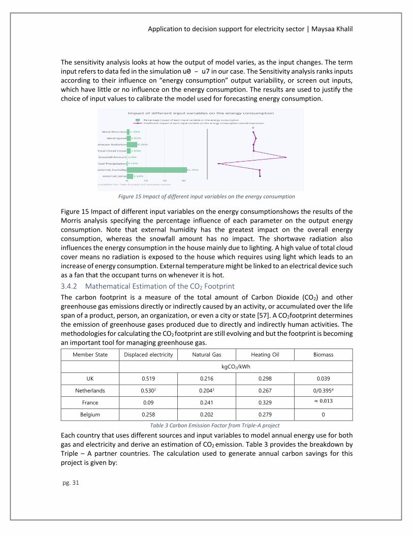
The sensitivity analysis looks at how the output of model varies, as the input changes. The term input refers to data fed in the simulation u0 – u7 in our case. The Sensitivity analysis ranks inputs according to their influence on “energy consumption” output variability, or screen out inputs, which have little or no influence on the energy consumption. The results are used to justify the choice of input values to calibrate the model used for forecasting energy consumption.

Figure 15 Impact of different input variables on the energy consumptionshows the results of the Morris analysis specifying the percentage influence of each parameter on the output energy consumption. Note that external humidity has the greatest impact on the overall energy consumption, whereas the snowfall amount has no impact. The shortwave radiation also influences the energy consumption in the house mainly due to lighting. A high value of total cloud cover means no radiation is exposed to the house which requires using light which leads to an increase of energy consumption. External temperature might be linked to an electrical device such as a fan that the occupant turns on whenever it is hot.

3.4.2 Mathematical Estimation of the CO2 Footprint

The carbon footprint is a measure of the total amount of Carbon Dioxide (CO2) and other greenhouse gas emissions directly or indirectly caused by an activity, or accumulated over the life span of a product, person, an organization, or even a city or state [57]. A CO2footprint determines the emission of greenhouse gases produced due to directly and indirectly human activities. The methodologies for calculating the CO2 footprint are still evolving and but the footprint is becoming an important tool for managing greenhouse gas.

Member State Displaced electricity Natural Gas Heating Oil Biomass

kgCO2/kWh

UK 0.519 0.216 0.298 0.039

Netherlands 0.5302 0.2043 0.267 0/0.3954

France 0.09 0.241 0.329 ≈ 0.013

Belgium 0.258 0.202 0.279 0

Table 3 Carbon Emission Factor from Triple-A project

Each country that uses different sources and input variables to model annual energy use for both gas and electricity and derive an estimation of CO2 emission. Table 3 provides the breakdown by Triple – A partner countries. The calculation used to generate annual carbon savings for this project is given by:

Figure 15 Impact of different input variables on the energy consumption


pg. 32

tCO2

a= [Energy demand prior to measure (kWh) − Energy demand post installation (kWh)]

× relevant emissions factor (kgCO2/ kWh) / 1000

The formula used to calculate CO2 emissions based on electrical consumption inside a house is as follows:

tCO2

a= [Energy consumption (kWh)] × relevant emissions factor (kgCO2/ kWh) / 1000

Yet, choices of the Triple-A project about the carbon emission factors with respect to each country may not be totally accurate. Thus, we decided to use values from the Réseau de Transport d'électricité (RTE13), that continuously provides an indicator of the carbon footprint of electricity generation in France, expressed in grams of CO2 per kWh generated.

Figure 16 Carbon footprint of hourly energy consumption

shows the estimation of CO2 footprint for each day of the 2018 year in our use case. The same peaks spotted in electric consumption, are spotted in the CO2 footprint. This shows that to decrease the CO2 footprint energy consumption must be reduced. Actions must be adopted especially in Christmas and some months in summer ( Figure 16 Carbon footprint of hourly energy consumption).

Figure 16 Carbon footprint of hourly energy consumption

3.5 Predicting Household Energy Consumption and CO2 Footprint

GREENHOME provides three energy forecast methods that use smart meters measurements and weather data to predict energy consumption in buildings. The pipeline implemented for studying energy consumption first applies the naïve forecast model, then the ARIMA model14, then the ARX model with other inputs that might decrease the performance gap. These models provide different perspectives of energy consumption in a household.

3.5.1 Naïve Forest Persistence Model

The naïve forecast persistence model15 consists in three steps: (i) preparing the dataset to create a lagged representation for each observation; (ii) using a resampling technique for splitting the dataset into train and/test fragments; (iii) measure performance to evaluate the model. e.g., mean squared error. The pseudocode of the function and its complexity is shown in Appendix B.

The persistence algorithm uses the value at time {t-1} to expect the predicted output at time {t}. The creation of a lagged representation of each observation means that given the record at

13 https://www.rte-france.com/ 14 We used this method because a significant difference is often observed between predicted performance and actual performance in the previous models. 15 https://www.sciencedirect.com/topics/engineering/persistence-model


pg. 33

{t-1}, the record at {t+1} is predicted. To fragment the dataset into training and test datasets we made a classification of 99% for training and 1% for testing. The persistence method can be defined as a function that returns the input provided.

The persistence model was evaluated on the test dataset using walk-forward validation method. The Walk-forward validation16 is a method where the model makes a prediction for each record in the dataset one at a time. Predictions were made for each record in the test dataset, the predictions were compared to the real values. The computed residual mean squared error was RMSE = 77.835.

The plot in Figure 17 Persistence forecast modelshows the training dataset and the diverging of the predicted line from the true values. Note that the model is a step behind the initial values. The graph is not stationary and varies a lot, which limits the persistence model.

The naïve forecast persistence model is a baseline for the forecast problem, that is, if any other forecast model achieves a performance at or below the baseline, the technique needs to be improved or abounded17.

3.5.2 ARIMA Model

An ARIMA model18 [58] was developed to solve the problem of forecasting household energy consumption. The model was configured both manually and automatically. At the end, residual error for the used ARIMA model was calculated. The standard notation is ARIMA(p, d, q)19 where p reflects the number of lag records included in the model, d reflects the degree of differencing, i.e. number of times the raw records is differenced and q reflects the order of moving average, which is the size of moving window. The pseudocode and complexity measures of the ARIMA model are shown in Appendix B Pseudocodes for Predicting Models Used.

Manual Configuration

ARIMA(p,d,q) requires the p, d & q parameters. Usually, the configuration is done manually.

The statsmodels.tsa.stattools.adfuller() method was used as a unit root to verify if data is stationary. As shown in Figure 18, the energy consumption data series is not-stationary.

16 https://en.wikipedia.org/wiki/Walk_forward_optimization 17 This is essential in the forecast problem because it gives an idea about how well all other models actually perform on the problem. 18 ARIMA is a class of statistical model for analyzing and forecasting time series data.

Figure 17 Persistence forecast model


pg. 34

Figure 18 Non-stationary plot of energy consumption

Therefore, a stationary version of the series is derived after differencing the original series followed by a test of stationary of the new data series. The unit root is done as a test for stationary. Unit root if found, then the time series is not stationary. The augmented Dickey-Fuller test gives a test statistic value -25.2, which is smaller than the critical value at 1% equal to -3.43. This accepts the rejection of the null hypothesis with a high level. The idea of rejecting the hypothesis confirms the fact that the process has no unit root, and therefore the series is stationary.

The difference between the test statistic value and the critical value is more than 20. Therefore, any value of d greater than 0 could be considered. This means that a differencing level of 2 can be used, and so d = 2. Now, both the lag values and the moving average parameters, p and q should be selected. These values can be derived from the autocorrelation function plots and the partial autocorrelation function plots. By default, all lag values are plotted, which is a noisy plot. This necessitates a definition of a good lag value, and as it is an hourly prediction, the best-chosen lag value is 25 since a similar consumption pattern happens at same hour of the previous day.

Figure 19 (left) shows autocorrelation graphs. The first graph is so condensed, with nothing to visualize. Therefore, as mentioned, a lag=25 is so significant to plot. The 2nd plot shows a correlation of 0.6 at lag=1, 0.4 at lag=2, and then 0.2 at lag=3. It is straightforward to see that lag=2 results in a good starting of p at 2.

Figure 19 Autocorrelation plot (left) & partial autocorrelation plot (right)

Figure 19 (right) presents the partial autocorrelation graph with lag=25, indicating a good starting value for q = 1. The graph shows a partial autocorrelation equal to 0.55 at lag=1, then it drops significantly to 0.1 at lag=2, then there is no correlation at t-2. The best value for q =


pg. 35

1. This analysis suggests a start with ARIMA(2,1,2) that gives an RMSE20 = 65.025 which is quite lower than the value generated by the persistence model.

Configuring ARIMA using Grid Search

To confirm the manual results, a grid search can be done to find best ARIMA parameters to ensure that no other combination can result in better RMSE performance. The search will skip values that will not converge. The values to search are: p: 0 to 4, d: 0 to 2, q: 0 to 4. This implied 300 runs of test harness, it took one hour to execute. Here, the ARIMA() function provided in the statsmodels.tsa.arima_model library, and the mean_squared_error() function provided by the sklearn.metrics library were used. The results shows that the best ARIMA model is ARIMA( 2, 1, 3) with an RMSE = 64.043, used next.

Review Residual Error

As a final validation of the chosen model, a review for the residual error forecast should be done. As an ideal case, the distribution of errors has to be a Gaussian distribution with zero mean. This can be checked by brief statistics and plots.

Count 102

Mean -0.348572

Std 64.358404

Min -153.106851

25% -44.182336

50% -4.695801

75% 28.659611

Max 241.561941

Table 4 Brief statistics for residual error

The mean is a non-zero value -0.5. This assures that the predictions are biased. The distribution of residual error is shown in Figure 20.

Figure 20 Distribution of residual error

The plot suggests a Gaussian-like distribution with a long middle tail. This information can be used to bias-correct prediction by adding -0.589739 to each forecast made. The predictions


pg. 36

performance changed from 64.043 to 64.042. Therefore, this bias correction can somehow be neglected, considering that the bias correction will increase complexity and cost without even increasing performance in the study case knowing that the performance did not change at all.

Model Validation

Once the model has been selected, it must be validated. The final RMSE value is equal to 64.121, which is not too far from previous calculated and expected value 64.043. Figure 21 shows a plot of each prediction and expected value for the time steps in the validation dataset. Some observations have (almost) the same values as the predicted ones whenever there was no significant deviation between one hour and the other. The model has a big performance gap whenever there is a sudden change in the hourly energy consumption. This calls for the addition of exogenous parameters as input to the forecast model to improve the forecast and reduce the performance gap and this is explained in the next section.

Figure 21 ARIMA Forecast Model plot

3.5.3 ARX Model

The ARX model is an autoregressive method with exogenous inputs (independent of the process being modelled)21. Autoregressive models express a univariate time series yn as a linear combination of past observations yn-1 and white noise Vn and is expressed mathematically as [59]:

𝑦𝑛 = ∑ 𝑎𝑖 . 𝑦𝑛−𝑖 + 𝑣𝑛

𝑚

𝑖=1

Where ai and m are the autoregressive coefficient and autoregressive order respectively.

Considering inputs rn and output Sn the ARX model can be expressed mathematically as [59]:

𝑠𝑛 = ∑ 𝑎𝑗 . 𝑠𝑛−𝑗 + ∑ 𝑏𝑗 . 𝑟𝑛−𝑗 +

𝑚

𝑗=1

𝑢𝑛

𝑚

𝑗=1

Where un is a white noise and aj and bj are p*p and p*q matrices respectively.

ARX can be useful and effective when the parameter to be estimated has a linear correlation with the input parameters of the algorithm. It is also effective for determining the order of the system. Thus, it is necessary to evaluate the order of the ARX polynomial to determine the order of the polynomial which results in the least cost and error. The AKAIKE criterion can be used to determine the most suitable order of the system [60]. The AKAIKE criterion is defined as an estimator of the relative quality of statistical models for a given set of data.

21 According to Diversi et al [66], ARX is the simplest model within the equation error family. It has many practical advantages concerning both estimations and predictive use since its optimal predictors are always stable.


pg. 37

Forecasting Energy Consumption with ARX

The external temperature, external humidity, wind direction, and total cloud coverage, were the exogeneous variables given as input for the forecast model of our experiment. This required the implementation of an autoregression model that considered the change of the electric consumption behavior according to the exogenous variables. Different input data were ingested into the model, out of which the following lead to the minimum RMSE value with highest performance in relation with the AKAIKE value being explained before. The linear regression expression went as follows, with y: consumption, u0: external temperature, u1: external humidity, u2: wind direction, u3: radiation, u4: wind speed.

Figure 22 ARX Forecast Model plotshows that the model forecasts a month and a half period of time and a high-performance gap with high peaks. Despite these issues, the forecast model successfully worked as shown hereafter.

Figure 22 ARX Forecast Model plot

For the RMSE, a manual check for best parameters using different input variables was done to test the model with different combinations. The above-mentioned combination of input variables led to the lowest RMSE = 55.843230.

3.6 Discussing Results

As what the results have proved, both models work as long as they produce an RMSE value less than the RMSE value produced by the baseline model, that is, the persistence model. However, ARX model has an RMSE value less than the ARIMA model, and this is so logical due to the fact that the ARIMA model does not take into consideration exogenous variables rather than previous observations as an input for its forecast model. The idea of measuring energy consumption is of great interest and is full of magic and weirdness because the energy consumption behavior is absolutely unpredictable. However, there are some cases where predictions can come true. The concept of predicting energy consumption without taking into consideration different indirect variables may work but not for all cases. Much more, indirect variables that impact energy consumption differs from one condition to another. For example, the house in the following case study uses electricity only for lighting, while other houses use electricity for heating. That is why, it seems nonsense to take into consideration the architecture of the house in the first case, but it can have a great impact in the second case.

y[k] = +0.537388 y[k − 1] + 0.240762 u0[k] + 0.503764 u1[k] + 0.010898 u2[k] + 0.035441 u3[k]

+ 0.105516 u4[k]


pg. 38

Chapter 4 Conclusion and Future Work The initial objective of this work was to propose a smart metering environment for predicting of energy consumption that will help in decreasing of the carbon footprint.

4.1 Main Results and Contribution

We have proposed GREENHOME, a smart metering energy and CO2 footprint environment, through which a toolkit for modeling and predicting energy consumption in households at different granularities and from different perspectives.

The environment was implemented on a house in Picardie, where electrical consumption was predicted using three different models: persistence model, ARIMA model, and ARX model after detecting anomalies to best fit the model on the given data. Carbon footprint was also estimated using some mathematical equations.

Given sensors data, the main aim was to predict energy consumption using the previous mentioned models and compare performances. The results show that the implemented ARX model, which adds exogenous variables as an input to the model, results in a less RMSE value and of better performance than the ARIMA model utilized. The inclusion of exogenous variables was made after doing a sensitivity analysis implemented using Morris method to check which variables impacts the most on the hourly consumption. External temperature and external humidity were the two most significant variables that affect the consumption.

4.2 Perspectives

Smart meter data analytics is a promising area that incorporates different field of science including the machine-learning field. Deciding which model to use in forecasting is a critical issue that is influenced by the requirements of the utility, the available sensor data, and the amount of data given. It is, without doubt, a topic that will grow more important as long as the smart grid topic is developing, where all parties involved should reap the environmental and economic benefits of progressing load forecasting and estimating the carbon footprint.

After being able to develop a machine-learning algorithm for predicting energy consumption inside buildings, and after being able to estimate the CO2 footprint of such consumption, I think that it is a crucial topic that needs to be taken into consideration to help decrease the effect of global warming.


pg. 39

Bibliography [1] E. Shove, “Beyond the ABC: Climate change policy and theories of social change,”

Environ. Plan. A, vol. 42, no. 6, pp. 1273–1285, 2010.

[2] A. C. Samli, “Toward a Model of International Consumer Behavior:,” J. Int. Consum. Mark., vol. 7, no. 1, pp. 63–84, 2005.

[3] J. L. Ramseur, “U . S . Carbon Dioxide Emissions in the Electricity Sector : Factors , Trends , and Projections SUMMARY U . S . Carbon Dioxide Emissions in the Electricity Sector : Factors , Trends , and Projections,” 2019.

[4] D. Elz, “Bioenergy systems,” Q. J. Int. Agric., vol. 46, no. 4, pp. 325–332, 2007.

[5] E. U. Building and S. Observatory, “Energy Performance of Buildings Directive,” Struct. Surv., vol. 23, no. 1, pp. 1–7, 2014.

[6] L. Suganthi and A. A. Samuel, “Energy models for demand forecasting - A review,” Renew. Sustain. Energy Rev., vol. 16, no. 2, pp. 1223–1240, 2012.

[7] A. Barghi, A. R. Kosari, M. Shokri, and S. Sheikhaei, “Intelligent lighting control with LEDS for smart home,” Smart Grid Conf. 2014, SGC 2014, pp. 1–5, 2014.

[8] N. K. Dhar, N. K. Verma, L. Behera, and M. M. Jamshidi, “On an Integrated Approach to Networked Climate Control of a Smart Home,” IEEE Syst. J., vol. 12, no. 2, pp. 1317–1328, 2018.

[9] S. U. Z. Khan, T. H. Shovon, J. Shawon, A. S. Zaman, and S. Sabyasachi, “Smart box: A TV remote controller based programmable home appliance manager,” 2013 Int. Conf. Informatics, Electron. Vision, ICIEV 2013, no. Iii, 2013.

[10] J. Bangali and A. Shaligram, “Design and implementation of security systems for smart home based on GSM technology,” Int. J. Smart Home, vol. 7, no. 6, pp. 201–208, 2013.

[11] M. Amayri, S. Ploix, and S. Bandyopadhyay, “Estimating Occupancy in an Office Setting,” pp. 72–80, 2015.

[12] Y. Wang, Q. Chen, T. Hong, and C. Kang, “Review of Smart Meter Data Analytics: Applications, Methodologies, and Challenges,” IEEE Trans. Smart Grid, no. June, pp. 1–24, 2018.

[13] H. X. Zhao and F. Magoulès, “A review on the prediction of building energy consumption,” Renew. Sustain. Energy Rev., vol. 16, no. 6, pp. 3586–3592, 2012.

[14] A. Foucquier, S. Robert, F. Suard, L. Stéphan, and A. Jay, “State of the art in building modelling and energy performances prediction: A review,” Renew. Sustain. Energy Rev., vol. 23, pp. 272–288, 2013.

[15] R. Mena, F. Rodríguez, M. Castilla, and M. R. Arahal, “A prediction model based on neural networks for the energy consumption of a bioclimatic building,” Energy Build., vol. 82, pp. 142–155, 2014.

[16] X. Lü, T. Lu, C. J. Kibert, and M. Viljanen, “Modeling and forecasting energy consumption for heterogeneous buildings using a physical-statistical approach,” Appl. Energy, vol. 144, pp. 261–275, 2015.

[17] A. Lomet, F. Suard, and D. Chèze, “Statistical Modeling for Real Domestic Hot Water Consumption Forecasting,” Energy Procedia, vol. 70, pp. 379–387, 2015.

[18] Z. Ma, H. Li, Q. Sun, C. Wang, A. Yan, and F. Starfelt, “Statistical analysis of energy


pg. 40

consumption patterns on the heat demand of buildings in district heating systems,” Energy Build., vol. 85, pp. 664–672, 2014.

[19] N. Fumo and M. A. Rafe Biswas, “Regression analysis for prediction of residential energy consumption,” Renew. Sustain. Energy Rev., vol. 47, pp. 332–343, 2015.

[20] F. Provost and T. Fawcett, “Authors’ Response to Gong’s, ‘Comment on Data Science and its Relationship to Big Data and Data-Driven Decision Making,’” Big Data, vol. 2, no. 1, pp. 1–1, 2014.

[21] Utility Analytics Institute, “The Current State of Smart Grid Analytics,” p. June 13, 2017.

[22] J. Lloret, J. Tomas, A. Canovas, and L. Parra, “An Integrated IoT Architecture for Smart Metering,” IEEE Commun. Mag., vol. 54, no. 12, pp. 50–57, Dec. 2016.

[23] L. Hernandez et al., “A survey on electric power demand forecasting: Future trends in smart grids, microgrids and smart buildings,” IEEE Commun. Surv. Tutorials, vol. 16, no. 3, pp. 1460–1495, 2014.

[24] J. Xie, T. Hong, and J. Stroud, “Long-term retail energy forecasting with consideration of residential customer attrition,” IEEE Trans. Smart Grid, vol. 6, no. 5, pp. 2245–2252, 2015.

[25] H. Chitsaz, H. Shaker, H. Zareipour, D. Wood, and N. Amjady, “Short-term electricity load forecasting of buildings in microgrids,” Energy Build., vol. 99, pp. 50–60, 2015.

[26] H. Shi, M. Xu, and R. Li, “Deep Learning for Household Load Forecasting-A Novel Pooling Deep RNN,” IEEE Trans. Smart Grid, vol. 9, no. 5, pp. 5271–5280, 2018.

[27] J. Yang et al., “k-Shape clustering algorithm for building energy usage patterns analysis and forecasting model accuracy improvement,” Energy Build., vol. 146, pp. 27–37, 2017.

[28] M. Adiba, J. A. Espinosa, and G. Vargas-solar, “Big Data Management Challenges , Approaches , Tools and their limitations To cite this version :,” no. February, 2016.

[29] R. Patgiri and A. Ahmed, “Big Data: The V’s of the Game Changer Paradigm V family of Big Data, All V’s of Big Data, Trends of Big Data, Redefinition of Big Data, Redefinition of Volume,” Proc. - 18th IEEE Int. Conf. High Perform. Comput. Commun. 14th IEEE Int. Conf. Smart City 2nd IEEE Int. Conf. Data Sci. Syst. HPCC/SmartCity/DSS 2016, no. April, pp. 17–24, 2016.

[30] H. Display, “Smart Meter / IHD,” no. I, pp. 1–15, 2011.

[31] S. Sendra, J. Lloret, M. García, and J. F. Toledo, “Power saving and energy optimization techniques for wireless sensor networks,” J. Commun., vol. 6, no. 6, pp. 439–459, 2011.

[32] A. Khameis, S. Rashed, A. Abou-Elnour, and M. Tarique, “Zigbee based optimal scheduling system for home appliances in the United Arab Emirates,” Netw. Protoc. Algorithms, vol. 7, no. 2, pp. 60–80, 2015.

[33] IEEE Smart Grid Working Group and IEEEWorking_Group, “Big Data Analytics in the Smart Grid Working Group on Big Data Analytics , Machine Learning and Artificial Intelligence in the Smart Grid,” IEE Smart grid, 2017.

[34] K. A. Heller and Z. Ghahramani, “Bayesian hierarchical clustering,” pp. 297–304, 2006.

[35] Y. Wang, Q. Chen, C. Kang, M. Zhang, K. Wang, and Y. Zhao, “Load profiling and its application to demand response: A review,” Tsinghua Sci. Technol., vol. 20, no. 2, pp. 117–129, 2015.

[36] T. K. Wijaya, M. Vasirani, and K. Aberer, “When bias matters: An economic assessment of


pg. 41

demand response baselines for residential customers,” IEEE Trans. Smart Grid, vol. 5, no. 4, pp. 1755–1763, 2014.

[37] M. Jaradat, M. Jarrah, A. Bousselham, Y. Jararweh, and M. Al-Ayyoub, “The internet of energy: Smart sensor networks and big data management for smart grid,” Procedia Comput. Sci., vol. 56, no. 1, pp. 592–597, 2015.

[38] Y. Weng and R. Rajagopal, “Probabilistic baseline estimation via Gaussian process,” IEEE Power Energy Soc. Gen. Meet., vol. 2015-Septe, 2015.

[39] S. Joseph, Jasmin E.A., and S. Chandran, “Stream Computing: Opportunities and Challenges in Smart Grid,” Procedia Technol., vol. 21, pp. 49–53, 2015.

[40] P. Deligiannis, S. Koutroubinas, and G. Koronias, “Predicting Energy Consumption Through Machine Learning Using a Smart-Metering Architecture,” IEEE Potentials, vol. 38, no. 2, pp. 29–34, Mar. 2019.

[41] M. K. Douglas C. Montgomery, Cheryl L. Jennings, Introduction to Time Series Analysis and Forecasting. 2011.

[42] P. A. Function, “Time Series,” vol. 52, no. 2, pp. 557–582, 2015.

[43] J. Peppanen, X. Zhang, S. Grijalva, and M. J. Reno, “Handling bad or missing smart meter data through advanced data imputation,” 2016 IEEE Power Energy Soc. Innov. Smart Grid Technol. Conf. ISGT 2016, 2016.

[44] JORG BREITUNG, “SOME SIMPLE TESTS OF THE MOVING-AVERAGE UNIT ROOT HYPOTHESIS,” vol. 15, no. 4, 1993.

[45] M. del C. Bas, J. Ortiz, L. Ballesteros, and S. Martorell, “Evaluation of a multiple linear regression model and SARIMA model in forecasting 7 Be air concentrations,” Chemosphere, vol. 177, pp. 326–333, 2017.

[46] Office of Electricity Delivery & Energy Reliability, “Advanced Metering Infraestructure and Customer Systems,” Results from Smart Grid Invest. grant Progr., p. 98, 2016.

[47] A. Mauri, A. Psyllidis, and A. Bozzon, “Social Smart Meter: Identifying Energy Consumption Behavior in User-Generated Content,” {WWW} (Companion Vol., pp. 195–198, 2018.

[48] L. Chapman, C. Bell, and S. Bell, “Can the crowdsourcing data paradigm take atmospheric science to a new level? A case study of the urban heat island of London quantified using Netatmo weather stations,” Int. J. Climatol., vol. 37, no. 9, pp. 3597–3605, 2017.

[49] H. Keemink, “Detecting central heating boiler malfunctions using smart- thermostat data,” TU Delft.

[50] B. Salina and P. Malathi, “An Efficient Data Fusion Architecture for Location Estimation Using FPGA,” vol. 3, no. 1, pp. 2634–2639, 2014.

[51] G. P. O. Box, N. Vincent, and U. François-rabelais, “for Two Biometric Applications,” vol. 00, no. c, pp. 18–21, 2006.

[52] Y. Hu, M. Lu, and X. Lu, “Spatial-Temporal Fusion Convolutional Neural Network for Simulated Driving Behavior Recognition,” 2018 15th Int. Conf. Control. Autom. Robot. Vision, ICARCV 2018, pp. 1271–1277, 2018.

[53] E. Picardie, “RENOVATION . PICARDIE . FR / PASS- RENOVATION / DYNAMISER-TERRITOIRE-,” pp. 1–6, 2019.

[54] The sean developers, “Docker Documentation,” no. 6.1.0.dev0, 2018.


pg. 42

[55] A. C. Davison and D. V. Hinkley, Bootstrap Methods And Their Application (Cambridge Series in Statistical and Probabilistic Mathematics), vol. 27, no. 3. 1997.

[56] W. Yu, B. Li, Y. Lei, and M. Liu, “Analysis of a residential building energy consumption demand model,” Energies, vol. 4, no. 3, pp. 475–487, 2011.

[57] E. J. GUMBEL, “Les valeurs extrêmes des distributions statistiques,” vol. 2, no. 5, pp. 115–158, 1935.

[58] S. W. Jefferson, “Modeling Large Forest Fires as Extreme Events Antecedents,” vol. 72, 1998.

[59] K. Modi and B. Oza, “Outlier Analysis Approaches in Data Mining,” Ijirt, vol. 3, no. 7, pp. 2349–6002, 2017.

[60] R. Baragona and F. Battaglia, “Projection Methods for Outlier Detection in Multivariate Time Series,” Sis-Statistica.It, no. 2000, pp. 107–118, 2004.

[61] D. Caro, “Carbon Footprint,” Encycl. Ecol., pp. 252–257, 2018.

[62] X. Wang and M. Meng, “A hybrid neural network and ARIMA model for energy consumption forecasting,” J. Comput., vol. 7, no. 5, pp. 1184–1190, 2012.

[63] Wikipedia, “Estimation Theory,” 2019. [Online]. Available: https://en.wikipedia.org/wiki/Estimation_theory.

[64] R. Diversi, R. Guidorzi, and U. Soverini, “Identification of ARX and ARARX Models in the Presence of Input and Output Noises,” Eur. J. Control, vol. 16, no. 3, pp. 242–255, 2010.

[65] Wikipedia, “Akaike Information Criterion (Aic) - Introduction.” [Online]. Available: https://en.wikipedia.org/wiki/Akaike_information_criterion.

[66] B. Iooss, P. Lemaître, B. Iooss, and P. Lemaître, “A review on global sensitivity analysis methods To cite this version : HAL Id : hal-00975701,” Algorithms Appl., 2015.


pg. 43

Appendix A Bad Data Detection Methods Bad data detection is one important step in data analysis that must be taken into consideration because training a model for forecast without treating bad data will generate wrong estimation and is a kind of bias.

Extreme Value Analysis

A box-and-whisker plot is used to identify outliers. The median is the middle number of a set of data. The median divides the data set into two parts, the upper set and the lower set. The lower quartile is the median of the lower half, and the upper quartile is the median of the upper half.

Data values very far away from the quartiles (either much less than lower quartile or much greater than upper quartile), it is sometimes designated an outlier.

Proximity Method

Proximity based techniques define a data point as an outlier, if its proximity is sparsely populated. To identify the proximity of a data point, several methods are used. The most common one is related to clustering.

The non-membership of a data point in any cluster, its distance from other clusters and size of the closest cluster are used to identify and compute the outlier score. The clustering problem has a complementary relationship to the outlier detection problem, out of which points belong to either clusters or outliers.

Figure 23 Box-and whisker plot for outlier detection

Figure 24 Anomaly detection with proximity method


pg. 44

As a first step, a clustering method is used to identify the natural clusters in the data. Then, the centroids of each cluster is defined and marked down. The distance from centroid to each data point in the cluster is measured in data space, if the distance exceeds a particular threshold, then the data point will be called as an outlier[55].

To measure the distance any appropriate distance measure can be used such as Manhattan distance, Euclidean distance, and Mahalanobis distance22. In this approach most-used algorithm is K-means algorithm which use Euclidean distance to find outliers.

Projection method: In a lower dimension projection method, a point is considered as an outlier if in some lower dimensional projection, it is present in a local region of abnormally low density.

The lower dimensional projection uses the proximity method explained before. Alternatively, another strategy is to compute the density of the local neighborhood of each point in low dimension. Then compute local outlier factor (LOF) of a sample p as the average of the ratios of the density of sample p and the density of its nearest local neighbors.

Outliers will be points with largest LOF values. In the normal approach, which is before projection, p2 is not considered as outlier, while LOF approach find p1 and p2 as outliers.

22 https://en.wikipedia.org/wiki/Mahalanobis_distance

Figure 25 Outlier detection in projection method


pg. 45

Appendix B Pseudocodes for Predicting Models Used Persistence Model and Complexity Measures

Input: D as a dataset containing columns related to a set of energy_consumption observation over a period of time (t).

1: For each observation(t) in the D

2: Create a lagged representation observation(t-1)

3: Separate dataset into train(70%) and test data set(30%)

4: Perform a persistence algorithm

5: model_persistence(x) = x

6: Evaluate the model

7: Use walk-forward validation method

8: For x in test_x

9: pr = model_persistence(x)

10: predictions.append(pr)

11: Calculate mean squared error.

Output: predictions of the end 30% period of t with a mean squared error for evaluation between predicted consumption and real one.

Complexity:

it requires O(1) space for every modification: just store the new data. Each modification takes O(1) additional time to store the modification at the end of the modification history.


pg. 46

ARIMA Model and Complexity Measures

Input: D as a dataset containing columns related to a set of energy_consumption observation over a period of time. 1: Plot D 2: While (graph is non_stationary = True) 3: smoothen graph to make it stationary 5: Find best level of differencing 6: d = best level of differencing 4: Plot ACF/PACF(Stationary_graph) 5: If ACF shows no lags 6: p = 0 7: else 8: p = nbre of lags 5: If PACF shows no lags 6: q = 0 7: else 8: q = nbre of lags 9: Grid search ARIMA hyperparameters 10: for p: 0 to 4 11: for d: 0 to 2 12: for q: 0 to 4 13: model = fit_model_ARIMA(p,d,q) 14: mse = evaluate_arima_model() 15: if mse < mse_initial 16: opt_model = model Output: ARIMA_model(p,d,q)

Measuring complexity:

Components for measuring complexity are as follows:

Ms = man hours of setting up the data and computer program for parameter estimation

C = computer use costs of analysis

MT = mans hour of interpreting and tabulating computer results

T = number of observations in the dataset

(p,d,q) = vector with components: p, order of the AR portion of the model, d, degree of differencing to achieve stationary, and q order of the MA portion of the model.

Ms, C, and MT are each positively related to T, p, d, and q

For simplicity, complexity costs will be measured as:

Ci = h.Ms + C + h.Mt

= h.Ms(T,p,d,q) + C(T,p,d,q) + h.MT(T,p,d,q)

Where h is the wage rate of the investigator

Ms ~ 𝛽1 + 𝛽2. 𝑇 + 𝛽3. (𝑝 + 2𝑞 + 1)

C ~ 𝛽4. 𝑇 + 𝛽5. (𝑝 + 2𝑞) + 𝛽6. 𝑇. (𝑝 + 2𝑞 + 1) + 𝛽7. 𝑇. (𝑝 + 2𝑞 + 1)2

MT ~ 𝛽8. (𝑝 + 2𝑞 + 1)


pg. 47

Comments:

Wherever q appears, it is multiplied by factor of 2. This is to incorporate the fact that moving average and mixed processes are more complicated than an autoregressive process.

For Ms, 𝛽1 reflects the time needed to write standard subroutines for the numerical computation of parameters of the marginal distribution, the time needed to write a program section transition from original dataset to the dth differences, and program debugging time. 𝛽2. 𝑇 time needed to tabulate and check data. 𝛽3. (𝑝 + 2𝑞 + 1) measures time needed to write p+q+1 integration routines.

For C, 𝛽4. 𝑇 measure costs of compiling data, printing predictions, and computing statistics. 𝛽5. (𝑝 + 2𝑞) reflects the cost of compiling the remainder of the program deck. 𝛽6. 𝑇. (𝑝 + 2𝑞 + 1) measures costs of computing predictions and obtaining plots of p+q+1 marginal. 𝛽7. 𝑇. (𝑝 + 2𝑞 + 1)2 measures cost of performing p+q+1 integrations.

For MT, 𝛽8. (𝑝 + 2𝑞 + 1) reflects the time needed to read and interpret the results of the analysis.


pg. 48

Appendix C Python Libraries Used In the following project, python was used as a programming language, where the following python libraries were used.

Pandas23, which is an open source, BSD-licensed library providing high-performance, easy-to-use data structures and data analysis tools for the Python programming language.

NumPy24, which is the fundamental package for scientific computing with Python. NumPy can also be used as an efficient multi-dimensional container of generic data.

Plotly25, which is a graphing library that makes interactive publication-quality graphs like line plots, scatter plots, area charts, bar charts, error bars, box plots, histograms, heatmaps, etc.

Matplotlib26, which is a Python 2D plotting library that produces publication quality figures in a variety of hardcopy formats and interactive environments across platforms.

Datetime27, which supplies classes for manipulating dates and times in both simple and complex ways.

Statsmodels28, which provides classes and functions for the estimation of many different statistical models, as well as for conducting statistical tests, and statistical data exploration.

Sklearn29, which is a simple and efficient tools for data mining and data analysis. It features various classification, regression and clustering algorithms including support vector machines, random forests, gradient boosting, k-means and DBSCAN, and is designed to interoperate with the Python numerical and scientific libraries NumPy and SciPy.

Math30, which provides access to the mathematical functions defined by the C standard.

Dash31, which is a Python framework for building analytical web applications.

SALib.analyze.morris32, which is a library that perform Morris analysis on model outputs.

23 https://pandas.pydata.org/ 24 https://www.numpy.org/ 25 https://plot.ly/ 26 https://matplotlib.org/ 27 https://docs.python.org/3/library/datetime.html 28 https://www.statsmodels.org/stable/index.html 29 https://scikit-learn.org/stable/ 30 https://docs.python.org/3/library/math.html 31 https://dash.plot.ly/ 32 https://salib.readthedocs.io/en/latest/_modules/SALib/analyze/morris.html


pg. 49

Appendix D Sensitivity Analysis and Correlation Study Morris Method

The Morris method for sensitivity analysis is a one-step-at-a-time (OAT) method for conducting sensitivity analysis. Thus, the algorithm varies one parameter at a time and evaluates the impact of that parameter. The Morris method was used because it is computationally inexpensive to implement. The main concept of the method is to discretize the input space for each variable and subsequently perform a specified number of OAT evaluations, the inputs for each step of OAT are randomly chosen and as such the direction of variation is also consequently random[61]. The repetition of these steps allows the estimation of elementary effects of each input and therefore, from these effects, sensitivity indices can be estimated. The Morris method classifies the input in three groups these are:

Inputs having negligible effects.

Inputs having large linear effects without interactions.

Inputs having large non-linear and/or interaction effects.

An example of Morris method is shown in Figure 26 Morris Method Example, which shows inputs affecting temperature inside a building.

Figure 26 Morris Method Example

Autocorrelation Plots

Autocorrelation is an important factor in data analysis. The correlation of a variable against a time-shifted version of the same variable is considered as autocorrelation. Autocorrelation can help


pg. 50

get information about repetitive events. Thus, autocorrelation can be used for identifying non-randomness in data and to classify an appropriate time series model for the non-random data. In other words, autocorrelation is considered as a correlation coefficient. Correlation here is not between two different variables. It is between different values of the same variable. If autocorrelation is used to spot non-randomness, first lag autocorrelation is taken into consideration. In order to determine a proper time series model, autocorrelation is plotted for various lags.

A first statistical test is considered here, the Pearson correlation coefficient, which produces a number to summarize how correlated two variables are. Values range between -1 (negatively correlated) and +1 (positively correlated) with small values close to zero to indicate low correlation, and values above 0.5 and below -0.5 to indicate high correlation. An example is illustrated in the following table.

t-1 t+1

t-1 1.000 0.5896

t+1 0.658 1.000

Another considered plots are the autocorrelation plots and the partial autocorrelation plot shown in Figure 27.

Figure 27 Autocorrelation Plot Example


pg. 51

Appendix E Smart Metering Applications & Environments A smart metering system consists in three main components:

(i) Smart meters installed in households that send data each 3,5,15 sec, etc. (ii) Communication networks to transmit data from and to the smart meters equipped in

the households. (iii) Data management system to store and process data, and send back data like billing

information, load forecast, real time carbon footprint, etc.

Social Smart Metering

Understanding energy consumption behavior is an important element in sustainable studies. Energy consumption related information could be extracted from user-generated content posted on social media. Such work was proposed in [62], where a pipeline helps identify energy-related terms in Twitter posts. Twitter posts were classified into four categories related to dwelling, leisure, food and mobility; according to the type of activity performed. A web-application was also developed that allows end users to check their energy consumptions based on analysis driven in the pipeline. The main thing that makes social media data trending is that traditional ways of getting data including smart meters is somehow costly and may lack contextual information.

Triple-A Environment

The focus will be on the use case in Picardie, as other use cases of the same environment have different applications with the same target in relation to energy efficiency. The system in Picardie was done in cooperation with QUARTUM. The different components of the environment are the following ones: (i) a sensor measuring/collecting electricity consumption (“electricity sensor”), (ii) a sensor measuring/collecting temperature and humidity outside (“weather sensor”), (iii) a sensor measuring/collecting temperature and humidity inside (“comfort sensor”), (iv) a sensor measuring/collecting gas consumption which is optional as not every household uses gas for heating (“gas sensor”), and (v) a tablet showing all the collecting data.

The sensors are wireless and works with batteries. The entire sensors collect data and send them to tablet which serves as a central data acquisition. Only the tablet needs to be connected to the power permanently as the tablet needs to be on for the data being collected. The information from the electricity sensor, the weather sensor and the gas sensor are sent via radio frequency (433 MHz) to the tablet and the comfort sensor sends its information to the tablet via Bluetooth.

On the tablet, in the HEMS33 application, you can see live information including (i) Electricity power in Watt, (ii) Live temperature and humidity inside the house, and (iii) Live temperature and humidity outside the house.

Information is stored in the tablet and presented through the tablet with different types of graphs. (i) For electricity: electricity load graphs, histograms with electricity consumption by day, weeks or months within a determined period, power distribution in a pie chart, distribution of consumption in terms of usage (i.e. lighting, cooking, heating, etc.), electricity meter index. (ii) For Gas: histograms with gas consumption by day, weeks or months within a determined period, gas meter index. (iii) For comfort: temperature curves, humidity curves, live comfort level,

33 HEMS home energy management system

http://quartum.eu/


pg. 52

distribution comfort history. (iv) General information: Information about equipment in the house, information about the house, information about family member.

NetatMo Application

It is an easily configured application controlled by a smartphone (or tablet) used to monitor and record the given local environment. NetatMo weather stations consist of a number of sensors, which monitor inside and outside air temperature (specified manufacturers accuracy: ±0.3∘C) and relative humidity (± 3%), as well as indoor barometric pressure (± 1mb), carbon dioxide concentration and noise pollution. Optional additional measurements include precipitation and wind, although these modules are less frequently purchased and therefore data are less available.

Data is transmitted wirelessly, using a combination of Bluetooth and Wi-Fi, to the cloud where it can be accessed via a smart device, as well as being made available online via a ‘weathermap’ on the NetatMo website with observations updated every 5 min[63].

TOON® Application

Toon® is a smart thermostat solution developed by Quby (a company based in Netherlands). The device offers a touch screen display through which users can set their preferences; Toon® is however not restricted to just thermal management, the device is capable of providing useful data on the building’s energy consumption and can also be used for security purposes. Toon ® is capable of interfacing with other smart devices such as smart plugs, Amazon Alexa® and Philips Hue Lighting ®. Toon® is an internet-connected device, thus allowing users remote access to change or update settings. Below is a summary of the specification of Toon®.

Utilities such as Eneco (Dutch utility) are also able to collect anonymous and aggregated data. This data is useful for scheduling, planning and allows end users to compare their usage patterns to similar households. Subsequently this data can be used to propose an optimized heating schedule[64].

Comparison

Table 5 shows some differences between the three mentioned environments and adds to the other environments.

Platform name System

type

Brief description Monitoring

capabilities

Control

capabilities

Out-of-

pocket

cost

Ongoing

cost

Triple-A Meter

board

system(can

be

connected

without

solar or

batteries)

IoT for electrical

and gas

monitoring with

thermal and

comfort

measuring.

Electricity and

gas

consumption

by day.

External

temperature

and humidity

curves.

None. Integrated

with Triple-

A team

Null

NetatMo Meter

board

system(can

be

Application used

to monitor and

record the given

local environment

Inside and

outside air

temperature,

relative

None Integrated

with

NetatMo

team

Null

https://www.toon.eu/explore-toon


pg. 53

connected

without

solar or

batteries)

with respect to

meteorological

data.

humidity,

indoor

barometric

pressure ,

carbon

dioxide

concentration

,noise

pollution

every 5

minutes

depending

on the

equipped

sensors

TOON Meter

board

system(can

be

connected

without

solar or

batteries)

Application used

for thermal

management,

building’s energy

consumption

monitoring and

providing security

purposes.

Real-time

visualization

of

temperature,

energy and

gas

consumption,

it shows when

the boiler is

working,

Select 4

different

temperature

modes and

create weekly

status for ideal

temperature34

Integrated

with TOON

company

Null

Enphase Home

Energy

Solution35

Inverter-

integrated

system

It coordinates

between solar,

batteries and

home energy

demand to

maximize overall

performance

Integrated

consumption

data is

visualized

every 15

minutes

-TOU36 tariff

optimization

Around

$600

installed

Null

Evergen37 Battery

Integrated

System

Developed by

CSIRO, it is an

intelligent

platform that

leams and

forecasts home

energy use and

solar production

Complete

home energy

monitoring

via Evergen

application

updated

every few

minutes

Interconnected

with home, grid

and energy

system, Evergen

manages home

energy to

decrease energy

bills

Integrated

with the

Evergen

team

$8 per

month

with

lock-in

contract

34 https://www.youtube.com/watch?v=jsyvEg36W30 35 https://enphase.com/fr-fr/produits-et-services/systemes-photovoltaiques 36 Time of use billings where electricity costs a different amount depending on the time of day it is used 37 https://www.evergen.com.au/


pg. 54

Redback

Technologies38

Inverter-

integrated

system

Smart inverter that

provides a fast

return on

investment by

decreasing

consumption

through intelligent

software

Multiple

circuit load

profiles in 1

minute

-IoT

-Inbuilt relay

control

-TOU

optimization

Free of

charge

Null

SMA Energy

meter39

Inverter-

integrated

system

3 phase energy

meter for

monitoring

consumption in

houses

Load curves

with 1 sec

polling

Non Around

$500

Null

SMA Sunny

Home

manager40

Inverter-

Integrated

system

Learning system

able to provide

prediction energy

generation and

load

recommendation

Complete

home energy

monitoring

every 5

minutes

Full system

control for SMA

PV and battery

inverters

Around

$500

Null

Wattwatchers41 Meter

board

system(can

be

connected

without

solar or

batteries)

IoT for energy

monitoring,

communications

(3G/LoRa/Wi-Fi)

and control of

electricity at circuit

level with real

time and historical

data.

5 sec live

data and 5

min stamped

energy data

Relay switches

and DRED

control

Around

$600

Monthly

charge

Table 5 Summary of existing environments

38 https://redbacktech.com/ 39 https://www.sma.de/en/products/monitoring-control/sma-energy-meter.html 40 https://www.sma.de/en/products/monitoring-control/sunny-home-manager-20.html 41 https://wattwatchers.com.au/

Master Thesis 2018-2019

Documents

Transcript of Master Thesis 2018-2019