MASTER THESIS 2010 - Fakultet for naturvitenskap - NTNU Master... · MASTER THESIS 2010 Title: The...
101
NTNU Faculty of Natural Sciences and Technology Norwegian University of Science Department of Chemical Engineering and Technology MASTER THESIS 2010 Title: The Drilling Process: A Plantwide Control Approach Subject (3-4 words): Drilling, optimization, plantwide, control Author: Dag-Erik Helgestad Carried out through: 12.01.2010 – 08.06.2010 Advisor: Professor Sigurd Skogestad Co-advisor: John-Morten Godhavn, Statoil ASA Main report: 63 pages Appendices: 25 pages + CD-ROM ABSTRACT Goal of work (key words): The goal of this thesis is to study the drilling process and create a simplified model based on drilling literature. The model should be used to optimize the drilling process based on total drilling costs for a set of given conditions. Further, we want to identify the optimal controlled variables for the drilling process. The self-optimizing controlled variables are variables that give the minimum loss when the process is subject to disturbances. Conclusions (key words): An extensive literature search was performed, covering the drilling process and the challenges involved. A steady-state model of the drilling process was created and used to optimize the drilling process for given parameters and conditions. The optimization of the drilling process was analyzed separately for the active drilling operations and pipe connections and drilling trips. The optimal controlled variables were identified using the method of maximizing the minimum singular value, the null space method and the exact local method. The results corresponded well with each other, identifying the weight on bit and the topdrive power as the optimal single measurement controlled variables. Research on avoiding stick-slip conditions during drilling support the conclusion of operating with a varying drill string rotational speed. Combining measurements will give a lower loss, but the loss is small (approximately 1% of the active drilling time) and the complexity of the control structure will increase. The savings compared to a constant input policy were relatively low, approximately 1% of the active drilling time. However, the drilling process is very expensive, and any savings in drilling time will equal a substantial revenue. The time spent during pipe connection- and drilling trip procedures is identified as an important factor in the optimization of the drilling process. A simple dynamic pressure model was used to simulate the performance of a automated feedback pressure control structure involving PI controllers. The control structure was able to perform the required procedures while keeping the bottom hole pressure within a pressure window of ±5 bar. I declare that this is an independent work according to the exam regulations of the Norwegian University of Science and Technology Date and signature: .......................................................
-
Upload
truongduong -
Category
Documents
-
view
212 -
download
0
Transcript of MASTER THESIS 2010 - Fakultet for naturvitenskap - NTNU Master... · MASTER THESIS 2010 Title: The...

NTNU Faculty of Natural Sciences and Technology Norwegian University of Science Department of Chemical Engineering and Technology
MASTER THESIS 2010 Title: The Drilling Process: A Plantwide Control Approach
Subject (3-4 words): Drilling, optimization, plantwide, control
Author: Dag-Erik Helgestad
Carried out through: 12.01.2010 – 08.06.2010
Advisor: Professor Sigurd Skogestad Co-advisor: John-Morten Godhavn, Statoil ASA
Main report: 63 pages Appendices: 25 pages + CD-ROM
ABSTRACT Goal of work (key words): The goal of this thesis is to study the drilling process and create a simplified model based on drilling literature. The model should be used to optimize the drilling process based on total drilling costs for a set of given conditions. Further, we want to identify the optimal controlled variables for the drilling process. The self-optimizing controlled variables are variables that give the minimum loss when the process is subject to disturbances. Conclusions (key words): An extensive literature search was performed, covering the drilling process and the challenges involved. A steady-state model of the drilling process was created and used to optimize the drilling process for given parameters and conditions. The optimization of the drilling process was analyzed separately for the active drilling operations and pipe connections and drilling trips. The optimal controlled variables were identified using the method of maximizing the minimum singular value, the null space method and the exact local method. The results corresponded well with each other, identifying the weight on bit and the topdrive power as the optimal single measurement controlled variables. Research on avoiding stick-slip conditions during drilling support the conclusion of operating with a varying drill string rotational speed. Combining measurements will give a lower loss, but the loss is small (approximately 1% of the active drilling time) and the complexity of the control structure will increase. The savings compared to a constant input policy were relatively low, approximately 1% of the active drilling time. However, the drilling process is very expensive, and any savings in drilling time will equal a substantial revenue. The time spent during pipe connection- and drilling trip procedures is identified as an important factor in the optimization of the drilling process. A simple dynamic pressure model was used to simulate the performance of a automated feedback pressure control structure involving PI controllers. The control structure was able to perform the required procedures while keeping the bottom hole pressure within a pressure window of ±5 bar.
I declare that this is an independent work according to the exam regulations of the Norwegian University of Science and Technology
Date and signature: .......................................................

ii

Preface
This master thesis was written during the spring of 2010 as a compulsory part of the studyprogram leading to a Master of Science (sivilingeniør) degree in Chemical Engineering at theNorwegian University of Science and Technology (NTNU). The thesis work has allowed me toexplore the field of drilling engineering and study the drilling process, while simultaneouslyincrease my knowledge in the field of process control. I have had a great learning profit and Iam sure that I will benefit of this thesis work in the future.
I would like to thank my supervisor for this project, Professor Sigurd Skogestad at the ProcessSystems Engineering group at NTNU, Trondheim, for support and guidance throughout thesemester. Equally, I wish to thank my co-supervisor at Statoil ASA, John-Morten Godhavn,who originally proposed the project and has been a valuable asset for advice. I would also like toextend my gratitude to PhD student Ramprasad Yelchuru at the Process Systems Engineeringgroup at NTNU, for taking the time to explain and help me understand the exact local method.
I would like to thank my fellow students Elisabeth Hyllestad, Martin Buus Jensen and AndersHaukvik Røed for keeping a good spirit and healthy, fun atmosphere at our office. It has beenhelpful to discuss our projects together and I very much enjoyed your company at coffee breaks.
Last but definitely not least, I would like to thank my parents, Riitta and Dag Helgestad. Yourlove and support (both moral and financial) has been an greatly appreciated throughout myyears as a student.
Dag-Erik HelgestadTrondheim, June 2010
iii

iv
Contents
List of Figures vii
List of Tables ix
List of Abbreviations xi
1 Introduction 11.1 Motivation . . . . . . . . . . . . . . . . . . . . . . . . . . . . . . . . . . . . . . . . 11.2 Aim and Scope of the Thesis . . . . . . . . . . . . . . . . . . . . . . . . . . . . . 2
2 Background 52.1 The Drilling Process . . . . . . . . . . . . . . . . . . . . . . . . . . . . . . . . . . 5
2.1.1 Managed Pressure Drilling (MPD) . . . . . . . . . . . . . . . . . . . . . . 62.2 Introduction to Numerical Optimization . . . . . . . . . . . . . . . . . . . . . . . 82.3 Control Structure Design (Plantwide Control) . . . . . . . . . . . . . . . . . . . . 9
2.3.1 Local Analysis . . . . . . . . . . . . . . . . . . . . . . . . . . . . . . . . . 112.3.2 Maximum Scaled Gain (Minimum Singular Value) Method . . . . . . . . . 122.3.3 Null Space Method . . . . . . . . . . . . . . . . . . . . . . . . . . . . . . . 132.3.4 Exact Local Method . . . . . . . . . . . . . . . . . . . . . . . . . . . . . . 14
2.4 PID Controller Design . . . . . . . . . . . . . . . . . . . . . . . . . . . . . . . . . 15
3 Steady-State Drilling Model 173.1 Drilling Model Equations . . . . . . . . . . . . . . . . . . . . . . . . . . . . . . . 17
3.1.1 The Rate of Penetration . . . . . . . . . . . . . . . . . . . . . . . . . . . . 173.1.2 Topdrive Torque and Power . . . . . . . . . . . . . . . . . . . . . . . . . . 193.1.3 Bottom Hole Cleaning . . . . . . . . . . . . . . . . . . . . . . . . . . . . . 193.1.4 Bottom Hole Pressure . . . . . . . . . . . . . . . . . . . . . . . . . . . . . 21
3.2 Parameters . . . . . . . . . . . . . . . . . . . . . . . . . . . . . . . . . . . . . . . 233.2.1 Parameters Relationships . . . . . . . . . . . . . . . . . . . . . . . . . . . 23
3.3 Drilling Model Results . . . . . . . . . . . . . . . . . . . . . . . . . . . . . . . . . 24
4 Optimization and Active Constraint Control 254.1 Degrees of Freedom (DOF) . . . . . . . . . . . . . . . . . . . . . . . . . . . . . . 254.2 Objective Function: The Cost of Drilling . . . . . . . . . . . . . . . . . . . . . . . 26
4.2.1 Bit Wear . . . . . . . . . . . . . . . . . . . . . . . . . . . . . . . . . . . . 274.2.2 Operating Modes . . . . . . . . . . . . . . . . . . . . . . . . . . . . . . . . 28
4.3 Operational Constraints . . . . . . . . . . . . . . . . . . . . . . . . . . . . . . . . 294.4 Optimization Results . . . . . . . . . . . . . . . . . . . . . . . . . . . . . . . . . . 304.5 Active Constraints . . . . . . . . . . . . . . . . . . . . . . . . . . . . . . . . . . . 314.6 Unconstrained Optimization . . . . . . . . . . . . . . . . . . . . . . . . . . . . . . 31
v

vi CONTENTS
5 Self-Optimizing Controlled Variables 335.1 Process Gains and Disturbances . . . . . . . . . . . . . . . . . . . . . . . . . . . . 345.2 Maximum Scaled Gain (Minimum Singular Value) Method . . . . . . . . . . . . . 355.3 Null Space Method . . . . . . . . . . . . . . . . . . . . . . . . . . . . . . . . . . . 365.4 Exact Local Method . . . . . . . . . . . . . . . . . . . . . . . . . . . . . . . . . . 375.5 Pairing of Variables . . . . . . . . . . . . . . . . . . . . . . . . . . . . . . . . . . . 405.6 Discussion . . . . . . . . . . . . . . . . . . . . . . . . . . . . . . . . . . . . . . . . 405.7 Stick-Slip Phenomenon . . . . . . . . . . . . . . . . . . . . . . . . . . . . . . . . . 42
6 Pressure Control and Automation 456.1 Pressure Control Structure . . . . . . . . . . . . . . . . . . . . . . . . . . . . . . . 466.2 Pipe Connections and Drilling Trips . . . . . . . . . . . . . . . . . . . . . . . . . 47
6.2.1 Automation with Controllers . . . . . . . . . . . . . . . . . . . . . . . . . 486.3 Dynamic Pressure Model . . . . . . . . . . . . . . . . . . . . . . . . . . . . . . . . 496.4 Simulations . . . . . . . . . . . . . . . . . . . . . . . . . . . . . . . . . . . . . . . 51
6.4.1 Controller Design . . . . . . . . . . . . . . . . . . . . . . . . . . . . . . . . 516.4.2 Results . . . . . . . . . . . . . . . . . . . . . . . . . . . . . . . . . . . . . 51
6.5 Discussion: Model Predictive Control (MPC) . . . . . . . . . . . . . . . . . . . . 55
7 Conclusions and Further Work 577.1 Conclusions . . . . . . . . . . . . . . . . . . . . . . . . . . . . . . . . . . . . . . . 57
7.1.1 Optimal Controlled Variables . . . . . . . . . . . . . . . . . . . . . . . . . 577.1.2 Pressure Control & Automation . . . . . . . . . . . . . . . . . . . . . . . . 58
7.2 Further work . . . . . . . . . . . . . . . . . . . . . . . . . . . . . . . . . . . . . . 59
Bibliography 60
A Nomenclature 65
B Miscellaneous Calculation Matrices 67
C Solving the Exact Local Method for a Multivariable Case 69
D Results of the Exact Local Method 71
E MATLAB files 75

List of Figures
1.1 The drilling rig Deepwater Horizon burning and sinking in the Gulf of Mexico . . 2
2.1 Schematic of an offshore drilling rig . . . . . . . . . . . . . . . . . . . . . . . . . . 62.2 Typical control system hierarchy in a chemical plant . . . . . . . . . . . . . . . . 102.3 Loss imposed by keeping a constant set point for the controlled variable . . . . . 112.4 Block diagram of a control structure with measurement combinations as controlled
variables . . . . . . . . . . . . . . . . . . . . . . . . . . . . . . . . . . . . . . . . . 13
4.1 Plots of the objective function J(u, d) vs the weight on bit (WOB) and the drillstring RPM . . . . . . . . . . . . . . . . . . . . . . . . . . . . . . . . . . . . . . . 32
4.2 Surface plot of the objective function J(u, d) versus the WOB and the drill stringRPM . . . . . . . . . . . . . . . . . . . . . . . . . . . . . . . . . . . . . . . . . . . 32
5.1 Plot of maximum loss versus the number of combined measurements . . . . . . . 385.2 Plot of maximum loss of optimal measurement combinations versus the magnitude
of disturbances . . . . . . . . . . . . . . . . . . . . . . . . . . . . . . . . . . . . . 395.3 Plot of maximum loss of poor measurement combinations versus the magnitude
of disturbances . . . . . . . . . . . . . . . . . . . . . . . . . . . . . . . . . . . . . 395.4 Plot of friction torque as a function of rotational speed of the drill string . . . . . 43
6.1 Schematic of a well, with the drilling mud circulation system . . . . . . . . . . . 466.2 Block diagram of the pressure control structure . . . . . . . . . . . . . . . . . . . 476.3 MATLAB Simulink switch block . . . . . . . . . . . . . . . . . . . . . . . . . . . 486.4 Block diagram of the pressure control structure with controllers for the main mud
pump flow rate and drill bit position . . . . . . . . . . . . . . . . . . . . . . . . . 496.5 Bottom hole pressure, main pump pressure, choke pressure and choke pressure set
point responses to a drilling trip simulation . . . . . . . . . . . . . . . . . . . . . 526.6 Close-up of the bottom hole pressure response in Figure 6.5 . . . . . . . . . . . . 526.7 Valve position response to a drilling trip simulation . . . . . . . . . . . . . . . . . 536.8 Main pump and drill bit flow rate response to a drilling trip simulation . . . . . . 536.9 Back pressure pump flow rate and choke flow response to a drilling trip simulation 546.10 Drill bit vertical position response to a drilling trip simulation . . . . . . . . . . . 546.11 Illustration of the MPD well control system with control hierarchy . . . . . . . . 55
vii

viii LIST OF FIGURES

List of Tables
2.1 Summary of Important Notation . . . . . . . . . . . . . . . . . . . . . . . . . . . 9
3.1 Penetration Rate Equation Parameters . . . . . . . . . . . . . . . . . . . . . . . . 183.2 Drilling Model Parameters . . . . . . . . . . . . . . . . . . . . . . . . . . . . . . . 233.3 Drilling Model Inputs . . . . . . . . . . . . . . . . . . . . . . . . . . . . . . . . . 243.4 Drilling Model Outputs . . . . . . . . . . . . . . . . . . . . . . . . . . . . . . . . 24
4.1 Manipulated Variables (MV’s) in the Drilling Process . . . . . . . . . . . . . . . . 264.2 Recommended Tooth-Wear Parameters for Rolling-Cutter Bits . . . . . . . . . . 284.3 Operational Constraints in the Drilling Process . . . . . . . . . . . . . . . . . . . 304.4 Nominal Optimal Values . . . . . . . . . . . . . . . . . . . . . . . . . . . . . . . . 304.5 Details About the Optimization . . . . . . . . . . . . . . . . . . . . . . . . . . . . 304.6 Active Constraints in the Drilling Process . . . . . . . . . . . . . . . . . . . . . . 31
5.1 Expected Disturbances . . . . . . . . . . . . . . . . . . . . . . . . . . . . . . . . . 345.2 Implementation Errors . . . . . . . . . . . . . . . . . . . . . . . . . . . . . . . . . 355.3 Optimal Variation, Implementation Errors and Expected Optimal Span . . . . . 355.4 Minimum Singular Value Results . . . . . . . . . . . . . . . . . . . . . . . . . . . 365.5 Optimal Controlled Variables . . . . . . . . . . . . . . . . . . . . . . . . . . . . . 38
6.1 Dynamic Pressure Model Parameters . . . . . . . . . . . . . . . . . . . . . . . . . 50
7.1 Optimal Controlled Variables . . . . . . . . . . . . . . . . . . . . . . . . . . . . . 58
A.1 Nomenclature . . . . . . . . . . . . . . . . . . . . . . . . . . . . . . . . . . . . . . 65
D.1 Optimal Combinations of 6 Measurements . . . . . . . . . . . . . . . . . . . . . . 71D.2 Optimal Combinations of 5 Measurements . . . . . . . . . . . . . . . . . . . . . . 71D.3 Optimal Combinations of 4 Measurements . . . . . . . . . . . . . . . . . . . . . . 72D.4 Optimal Combinations of 3 Measurements . . . . . . . . . . . . . . . . . . . . . . 73D.5 Optimal Combinations of 2 Measurements . . . . . . . . . . . . . . . . . . . . . . 74
E.1 List of MATLAB Files . . . . . . . . . . . . . . . . . . . . . . . . . . . . . . . . . 75
ix

x LIST OF TABLES

List of Abbreviations
BHA Bottom hole assemblyBHP Bottom hole pressureBOP Blow-out preventerCV Controlled variableDOF Degree(s) of freedomMPC Model Predictive ControlMPD Managed Pressure DrillingMV Manipulated variableMWD Measurement While DrillingPI Proportional-integral (controller)PID Proportional-integral-derivative (controller)QP Quadratic programRCD Rotating Control DeviceROP Rate of penetrationRPM Revolutions per minuteRTO Real-time OptimizerSQP Sequential quadratic programmingWOB Weight on bit
xi

xii LIST OF ABBREVIATIONS

Chapter 1
Introduction
1.1 Motivation
According to the International Energy Agency (IEA), the world energy demand is expected toincrease by 44% from 2006 to 2030.[1] At the same time, most of the easily-attained petroleumreserves are already exploited. The result is that the petroleum industry is facing technicalchallenges in most areas of the upstream industry. The remaining reservoirs are smaller, deeperand in more remote locations than the typical reservoir of the previous decades. There is aneed for accurate, cost-effective drilling systems capable of drilling complex wells with increaseddemands on pressure control.
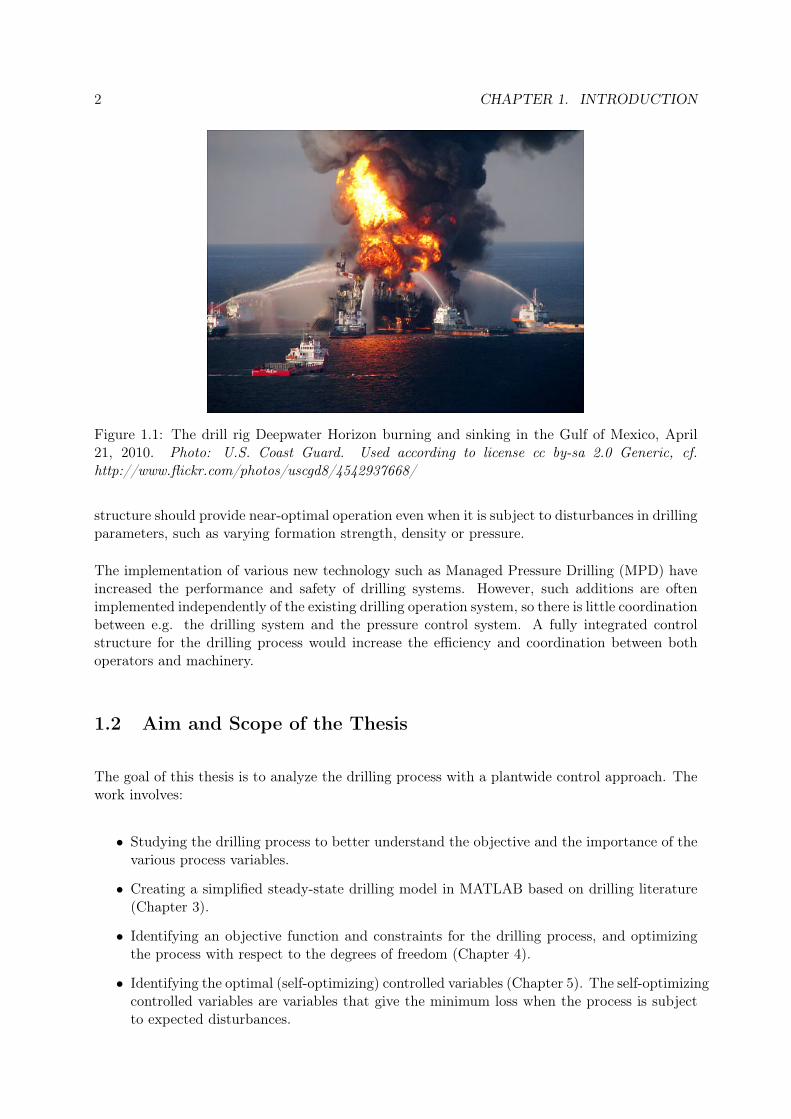
The process of drilling a well is very expensive, as it involves hiring a drilling rig and crew forthe duration of drilling the well. It is therefore important to drill the well as fast as possiblein order to minimize the cost. The drillers are highly experienced and aim to drill fast andsafe, while keeping within a set of boundaries and handling upsets. However, the drilling processinvolves coordinating a lot of machinery and making quick decisions with the possibility of severeconsequences. The catastrophic blowout on the drill rig Deepwater Horizon in the Gulf of Mexicoin April 2010 clearly showed the magnitude of the potential dangers. The blowout led to theburning and sinking of the drill rig (see Figure 1.1), and an oil leak with huge environmentalimpact. Naturally, the situation became the focus of world press and political agendas, as wellas having enormous economical consequences for the responsible companies.
Many of the decisions made on the rig floor require extremely good knowledge of the variouseffects in the drilling process, and they should be made faster than what is possible for a human.Also, the decisions are often based on experience and out-dated industry standards which arenot necessarily optimal for each and every purpose. Therefore, the drilling process has greatpotential for increased automation and optimization in terms of process control.
The downstream industry is highly dependent on good process control, as the refinery productspecifications are controlled very tightly. The application of properly designed control structuresand properly tuned controllers has increased the regularity and thus the profit margins of refineryproducts. It is desirable to analyze the drilling process using a plantwide control approach,in order to determine the optimal variables to control during drilling. The resulting control
1
2 CHAPTER 1. INTRODUCTION
Figure 1.1: The drill rig Deepwater Horizon burning and sinking in the Gulf of Mexico, April21, 2010. Photo: U.S. Coast Guard. Used according to license cc by-sa 2.0 Generic, cf.http://www.flickr.com/photos/uscgd8/4542937668/
structure should provide near-optimal operation even when it is subject to disturbances in drillingparameters, such as varying formation strength, density or pressure.
The implementation of various new technology such as Managed Pressure Drilling (MPD) haveincreased the performance and safety of drilling systems. However, such additions are oftenimplemented independently of the existing drilling operation system, so there is little coordinationbetween e.g. the drilling system and the pressure control system. A fully integrated controlstructure for the drilling process would increase the efficiency and coordination between bothoperators and machinery.
1.2 Aim and Scope of the Thesis
The goal of this thesis is to analyze the drilling process with a plantwide control approach. Thework involves:
• Studying the drilling process to better understand the objective and the importance of thevarious process variables.
• Creating a simplified steady-state drilling model in MATLAB based on drilling literature(Chapter 3).
• Identifying an objective function and constraints for the drilling process, and optimizingthe process with respect to the degrees of freedom (Chapter 4).
• Identifying the optimal (self-optimizing) controlled variables (Chapter 5). The self-optimizingcontrolled variables are variables that give the minimum loss when the process is subjectto expected disturbances.

1.2. AIM AND SCOPE OF THE THESIS 3
The steady-state optimization and identification of optimal controlled variables assumes that thetime spent making pipe connections and drilling trips is constant. However, pipe connectionsand drilling trips are recognized as important operations in terms of minimizing the total drillingtime. Therefore, an additional study of the performance of feedback pressure control structureis performed (Chapter 6).

4 CHAPTER 1. INTRODUCTION

Chapter 2
Background
This section will introduce the process of drilling a well for petroleum production, including theequipment used and challenges that are faced. The first section will describe the traditional setupof a drilling rig, while the purpose and design of a Managed Pressure Drilling (MPD) systemis described in the succeeding section. The last sections include an introduction to numericaloptimization and an introduction to control structure design (plantwide control), as well as adescription of PID controllers.
2.1 The Drilling Process
The drilling of wells into petroleum reserves is performed by a drilling rig, such as illustrated inFigure 2.1. The drilling rig in the figure is a jacket platform used in offshore drilling operations.The drill string with the drill bit at the end is rotated by the topdrive, an electric motor at thetop end of the drill string. The topdrive is attached to a hook in the derrick, making it possible toraise and lower the drill string by the drawworks (hoisting system). While drilling, the drill stringis lowered due to the weight of the string and the progress of the drill bit. As the position of thetopdrive reaches the bottom of the derrick, a new stand of drill pipe added and the hook positionis moved to the top of the new connection. Each stand of pipe is approximately 27 meters inlength, so a typical penetration rate of 15 m/hr will require a new connection approximatelyevery other hour.[2]
Although not clearly illustrated in Figure 2.1, the drilling rig contains a mud circulation system.The drilling mud is pumped through the drill string to the bottom of the well and returns tothe surface through the well annulus. The cuttings are separated from the returning mud inshale shakers, and the mud is sent back to mud tanks on the drill rig. The main functions of thedrilling mud are to:
• Provide hydrostatic pressure to the well to prevent formation fluids from entering the wellduring drilling.
• Transport the rock cuttings away from the bit (to ensure efficient drilling) and back to thesurface through the well annulus.
5

6 CHAPTER 2. BACKGROUND
Figure 2.1: Offshore drilling rig (jacket platform). Drilling mud flows from the main pumpthrough the drill string, out of the bit and back up in the well annulus. The mud transports therock cuttings out of the well, and also provides hydrostatic pressure to the borehole.[2]
• Keep the drill bit cool and clean during operation.
Drilling muds also have special properties allowing them to suspend the cuttings while drillingis paused and the mud is stationary. Various drilling muds have even more specific functions,such as sealing permeable formations, controlling corrosion and facilitating cementing, but theseeffects will not be covered in this thesis.
2.1.1 Managed Pressure Drilling (MPD)
Figure 2.1 of the example drilling rig shows that the top of the annulus is sealed off by a rotatingcontrol device (RCD). The RCD is a part of a newer, more sophisticated drilling technology calledManaged Pressure Drilling (MPD). In conventional drilling, the mud return is open, meaning itreturns to atmospheric pressure. With the implementation of a RCD, the returning mud mustexit through a choke valve, and the valve opening may be controlled by the drillers. This systemprovides a means for controlling the pressure profile in the well annulus, which is very importantfactor in achieving effective drilling. It is important to keep the pressure profile within thepressure window, which depends on the characteristics of the formation.
The pressure in the well must be above the collapse pressure of the borehole, to prevent the borehole from catastrophically closing in due to the differential pressure acting from outside to insideof the well. Similarly it is important to keep the pressure below the fracturing pressure of the

2.1. THE DRILLING PROCESS 7
bore hole, in order to prevent hydraulic fracture of the rock formation. Another important aspectof well pressure control is to prevent uncontrolled influx of reservoir fluids or loss of drilling mudinto the formation. In the case of too low pressure, formation fluids may flow into the annulusand be driven towards the surface by the pressure gradient. This phenomenon is called a drillingkick, and is often encountered during drilling. In the worst case, a kick may lead to a surfaceblowout, causing large financial losses and possible damages to environment and human lives. Ifthe well pressure is higher than the formation pressure, the drilling mud will flow into the porousreservoir and possibly clog up the pores. Drilling mud is fairly expensive, so losses are certainlyundesirable, but the loss of mud may also restrict the production from that part of the reservoir.
The pressure in the annulus is mainly affected by the hydrostatic weight of the mud, but alsothe pressure that arises due to friction losses when the mud is circulated. The RCD and chokevalve make it possible for the drillers to set a pressure at the top of the annulus by manipulatingthe choke valve opening. The annulus pressure profile will be affected by the pressure at the top,thus facilitating control of the bottom hole pressure (BHP). In addition to the choke valve, thetop side of the annulus is also connected to a back pressure pump. This pump is included tohelp the choke valve provide the required pressure, as the choke valve naturally is restricted toits fully closed and fully open positions.
Being able to apply a pressure at the top of the annulus reduces the risk of drilling kicks leadingto a blowout, as the kick may be countered by increasing the choke pressure. The advantage isthat we are able to drill underbalanced, in other words with a bottom-hole pressure that is lowerthan the formation pressure. Underbalanced drilling increases the rate of penetration, eliminatesformation damage because no mud is forced into the formation, reduces lost circulation andeliminates differential sticking. However, it is critical that the pressure control system is reliable.
Several procedures during drilling operations have significant effects on the annulus pressure.Each time a pipe connection is made, the main pump is disconnected and circulation stops. Thepressure term due to friction is thereby lost. Changing the drill bit or other failures requirea full retraction of the drill string from the well, called a drilling trip. The volume of thewell is increased, leading to a lower mud height and pressure. The opposite (a pressure surge) isexperienced when inserting the drill string back into the well. Similar effects of vertical movementof the drill string are experienced in offshore drilling due to wave motion (heave).
It is clear that accurate control of the annulus pressure profile is important during all aspectsof the drilling process. In Managed Pressure Drilling (MPD) control structures, the bottomhole pressure (the pressure at the drill bit) or the shoe pressure (the pressure at the bottom ofthe casing, above the openhole section) is usually chosen as the controlled variable. However,the downhole pressures are not easily measured. Information from the bottom of the well istraditionally sent to the surface by pulses in the mud (mud-pulse telemetry). These signalsare not available when the mud circulation rate is low or stopped completely, e.g. during pipeconnections. Instead, advanced hydraulic models have been used to estimate the downholepressures. Stamnes [2] studied the estimation of the bottom hole pressure (BHP) using adaptiveobservers. For the course of this thesis we however assume a wired drill string with exactmeasurement of the bottom hole pressure.
8 CHAPTER 2. BACKGROUND
2.2 Introduction to Numerical Optimization
Optimization problems are seen in various applications, such as stock portfolios, chemical pro-cesses and transportation logistics. Optimization is also present in various levels of typicalindustry companies, from management to design to operation. The purpose of any optimizationis to find the values of the variables corresponding to the best possible value of a given objectivefunction. An optimization problem function can be linear or non-linear, and may be subject toconstraints. A general optimization problem can be defined as follows:
Minimize (or maximize): J = f(x) (2.1)Subject to: g(x) ≤ 0
h(x) = 0
In Equation 2.2, J represents the objective function, which is a function of variable(s) x. Theoptimization problem may be subject to inequality constraints g(x) and equality constraints h(x).
Different optimization methods have been developed in order to solve problems such as above. Inthe case where both objective function and constraints are linear functions of the variables, theoptimization becomes a linear programming problem. If either objective function or constraintsare non-linear functions of the variables, the problem is non-linear and more sophisticated meth-ods are required to solve the problem.
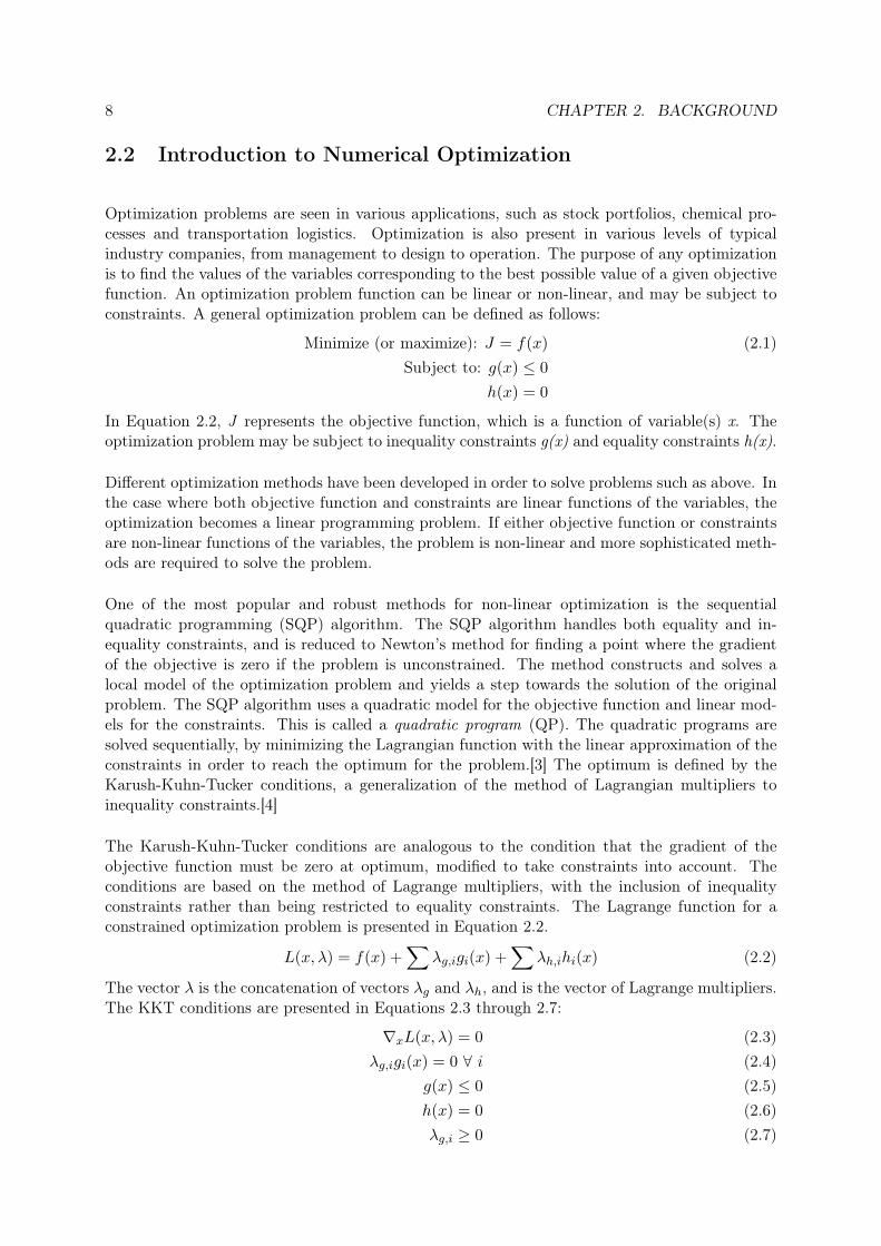
One of the most popular and robust methods for non-linear optimization is the sequentialquadratic programming (SQP) algorithm. The SQP algorithm handles both equality and in-equality constraints, and is reduced to Newton’s method for finding a point where the gradientof the objective is zero if the problem is unconstrained. The method constructs and solves alocal model of the optimization problem and yields a step towards the solution of the originalproblem. The SQP algorithm uses a quadratic model for the objective function and linear mod-els for the constraints. This is called a quadratic program (QP). The quadratic programs aresolved sequentially, by minimizing the Lagrangian function with the linear approximation of theconstraints in order to reach the optimum for the problem.[3] The optimum is defined by theKarush-Kuhn-Tucker conditions, a generalization of the method of Lagrangian multipliers toinequality constraints.[4]
The Karush-Kuhn-Tucker conditions are analogous to the condition that the gradient of theobjective function must be zero at optimum, modified to take constraints into account. Theconditions are based on the method of Lagrange multipliers, with the inclusion of inequalityconstraints rather than being restricted to equality constraints. The Lagrange function for aconstrained optimization problem is presented in Equation 2.2.
L(x, λ) = f(x) +∑
λg,igi(x) +∑
λh,ihi(x) (2.2)
The vector λ is the concatenation of vectors λg and λh, and is the vector of Lagrange multipliers.The KKT conditions are presented in Equations 2.3 through 2.7:
∇xL(x, λ) = 0 (2.3)λg,igi(x) = 0 ∀ i (2.4)
g(x) ≤ 0 (2.5)h(x) = 0 (2.6)λg,i ≥ 0 (2.7)

2.3. CONTROL STRUCTURE DESIGN (PLANTWIDE CONTROL) 9
Equation 2.3 represents the condition of a zero gradient of the Lagrangian function, while Equa-tion 2.4 represents the complementary slackness. Equations 2.5 and 2.7 require that the in-equalities and equalities constraints are met, while Equation 2.7 requires that the Lagrangianmultipliers associated with the inequality constraint functions are positive.[4]
2.3 Control Structure Design (Plantwide Control)
Control structures in the chemical industry are often organized in a hierarchy as illustrated inFigure 2.2.[5] As indicated in the figure, the two bottom layers are parts of the control structure,while the layers above provide the operational setpoints for the process. In order to design acontrol structure one must carefully analyze the process at hand. A lot of work may be put intodesigning and tuning controllers, but the control structure itself may be far from optimal for itspurpose. This section will present the procedures of Skogestad et al. [5, 6, 7, 8, 9, 10] for controlstructure design and selection of self-optimizing controlled variables. A summary of importantnotation is presented in Table 2.1.
Table 2.1: Summary of Important Notation
u Unconstrained degree of freedom (MV)y Measurement (including u’s)z Controlled variable (CV)nu # of u’snz # of CV’s (nz = nu)ny # of y’s (ny ≥ nz)
J(u, d) Cost function to be minimizedJopt(d) Optimal value of J
L = J(u, d) - Jopt(d) Loss
The plantwide control approach to a control structure design problem is based on top-down andbottom-up procedures. The top-down analysis is used to determine the controlled outputs, whilethe bottom-up procedures are used to select measurements and manipulated variables as well asdetermine a control configuration. The procedures are summarized below. [5]
Top-down:
1. Identify a cost function J for the process and identify operational constraints.
2. Identify the degrees of freedom available to the process.
3. Analayze the solution for optimal operation for various disturbances, with the purpose ofdetermining the primary controlled variables (CV’s) which, when kept at a constant setpoint, indirectly minimize the cost.
Bottom-up:
1. Regulatory control: Identify additional variables to be measured and controlled, and suggestpairing with manipulated inputs.

10 CHAPTER 2. BACKGROUND
Figure 2.2: Typical control system hierarchy in a chemical plant.[5]
2. Supervisory control: Propose a configuration for a supervisory control layer (decentralized,MPC).
3. On-line optimization: Determine whether a real-time optimizer (RTO) is needed, or whetherconstant setpoints are sufficient.
The top-down procedures with selection of the controlled variables is the most critical part ofthe plantwide control approach. After optimizing with respect to the objective function J andthe operational constraints, we get the nominal optimal values for the manipulated variablesor inputs (u), and the measurements (y). The next step is to determine the optimal controlledvariables (CV’s), also denoted as z. First, active constraints must be controlled to ensure optimaloperation. One degree of freedom (manipulated variable) is consumed for control of each activeconstraint. Further, we want to choose the best possible CV’s to control with the remainingmanipulated variables. We want to choose CV’s that, when controlled at a constant set point,give minimal loss when the process is subject to disturbances. The optimal CV’s are thereforecalled self-optimizing controlled variables. The idea is illustrated in Figure 2.3, where z1 is abetter controlled variable than z2.
The self-optimizing controlled variables may be determined by performing so-called brute-forceanalyses. This involves selecting various combinations of controlled variables, introducing ex-tected disturbances and calculating the loss. However, in most cases we have many measurementsto choose from but only a few manipulated variables, which leads to very many combinations ofCV’s. Therefore, we use mathematical methods to determine the best controlled variables. Wewill perform a local analysis of the loss function to explain the theory.

2.3. CONTROL STRUCTURE DESIGN (PLANTWIDE CONTROL) 11
Figure 2.3: Loss imposed by keeping a constant set point for the controlled variable. In this casez1 is a better self-optimizing controlled variable than z2.[5]
2.3.1 Local Analysis
The loss function is the difference between the cost function J(u, d) and the re-optimized costfunction Jopt(u, d), where d represents a disturbance to the system. The cost function J(u, d)is assumed to be twice differentiable, and the optimization problem is considered to be uncon-strained. Any active constraints should have been removed (both the measurement and onedegree of freedom) from further analysis as described above. We want to determine which vari-ables are best to control by the remaining manipulated variables.
The objective function may be expressed as a local second-order Taylor series expansion aroundthe nominal optimal point of operation. This is shown in Equation 2.8.
J(u, d) = Jopt(u, d) +[Ju Jd
]T [∆u∆d
]+
12
[∆u∆d
]T [Juu Jud
Jdu Jdd
] [∆u∆d
](2.8)
where ∆u = u−uopt and ∆d = d−dopt. We recognize that the gradient of the objective functionwith respect to the manipulated variables (Ju) is equal to zero at the unconstrained optimum.For a given disturbance d (∆d = 0), the loss function may be written as Equation 2.9.
L = J − Jopt =12
(u− uopt)TJuu(u− uopt) (2.9)
Introducing z = J1/2uu (u−uopt), we may reduce the notation to Equation 2.10. ‖z‖2 is the 2-norm,
or maximum singular value of z.
L =12‖z‖22 (2.10)

12 CHAPTER 2. BACKGROUND
2.3.2 Maximum Scaled Gain (Minimum Singular Value) Method
The controlled variables (z) are chosen as a subset of the available measurements (y). Thecontrolled variables (z) may be expressed as a function of the manipulated variables (u) and thedisturbances (d) as shown in Equation 2.11.
z = Gu+Gdd (2.11)
Assuming that the disturbance d is fixed (∆d = 0), we may write z − zopt = G(u − uopt).Equation 2.12 shows how z − zopt can be written as a sum of an optimization error eopt and animplementation error n.
z − zopt = z − r + r − zopt = n+ eopt(d) (2.12)
The optimization error is the difference between the optimal value zopt and the set point for thecontroller r (the nominal optimal value). The implementation error is the difference betweenthe controller set point and the actual value of z. The implementation error is due to imperfectcontrol, or due to incorrect measurements, which often are a factor i real systems. The absolutevalue of z−zopt is called the expected optimal span of the measurements, and is denoted span(z).
For a multivariable case, z and u are vectors. According to Skogestad & Postlethwaite [5], theoutputs are scaled with respect to their optimal span by multiplication with the output scalingmatrix S1 = diag{1/span(zi)}. The resulting scaled outputs are shown in Equation 2.13, whereG′ = S1G.
z′ − z′opt = S1G(u− uopt) = G′(u− uopt) (2.13)
Using (u− uopt) = G′−1(z′ − z′opt) and Equation 2.10, we write Equation 2.14.
L =12||J1/2
uu G′−1(z′ − z′opt)||22 (2.14)
The scaled output deviation z′ − z′opt has a magnitude of less than unity due to the scaling.Therefore, the maximum value of the 2-norm ‖z′ − z′opt‖2 is unity. The maximum expected lossfor a multivariable case may then be expressed as in Equation 2.15.[5]
Lmax = max‖z′−z′opt‖2≤1
12||J1/2
uu G′−1(z′ − z′opt)||22
=12σ2(J1/2
uu G′−1) =
12
1
σ2(G′J−1/2uu )
(2.15)
The maximum of the 2-norm ‖z‖2 is given by the induced 2-norm ‖J1/2uu G′−1‖i2, which is equal to
the maximum singular value σ(J1/2uu G′−1). The last equality is given by the relationship between
the maximum and minimum singular values, as shown in Equation 2.16.
σ(A−1) = 1/σ(A) (2.16)

2.3. CONTROL STRUCTURE DESIGN (PLANTWIDE CONTROL) 13
From Equation 2.15 we can deduce that it is optimal to choose measurements that maximize theminimum singular value σ(G′J−1/2
uu ), where G′ = S1G.
2.3.3 Null Space Method
We have considered z as a subset of the available measurements y. However, if we use linearcombinations of measurements y to form various z’s, we have an infinite number of potentialcontrolled variables available.[5, 10] We express z as shown in Equation 2.17. A block diagramof a control structure with measurement combinations is presented in Figure 2.4.
z = Hy (2.17)
Figure 2.4: Block diagram of a control structure with measurement combinations as controlledvariables.[9] Note: The controlled variables are denoted c in the figure, while this thesis usesnotation z.
The re-optimized values of the measurements (yopt) depend on the disturbance that is introducedon the system. They also depend on the implementation error (see Equation 2.12), but for thiscase we assume that the implementation errors are negligible. We may express this relationshipas shown in Equation 2.18. The matrix F may be viewed as the gain from the disturbance d tothe optimal variation of the measurements.
∆yopt = F ∆d (2.18)
Optimally, we want zopt to be independent of the disturbance d (∆zopt = 0 · ∆d). CombiningEquation 2.17 with Equation 2.18, we get Equation 2.19.
∆zopt = HF∆d (2.19)
In order to achieve optimal constant set points (zopt = 0), we require that HF = 0. In otherwords, H must be in the left null space of F . The null space of F has dimension ny − nd so we
14 CHAPTER 2. BACKGROUND
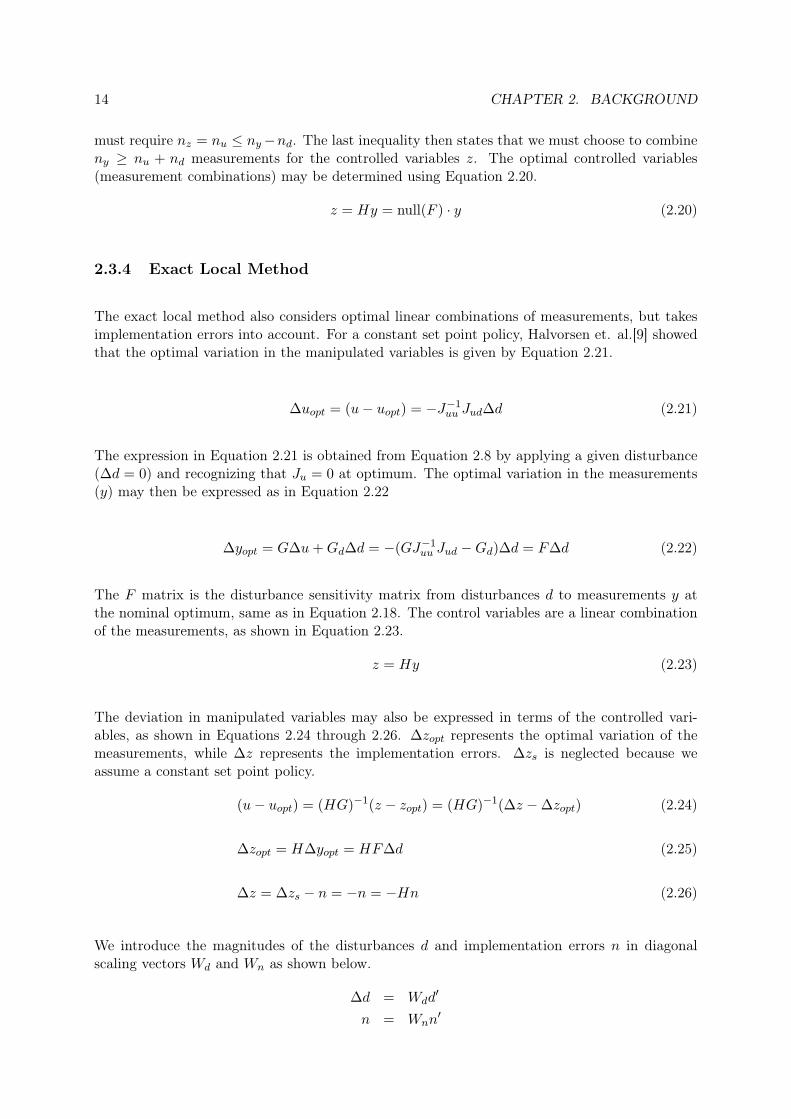
must require nz = nu ≤ ny−nd. The last inequality then states that we must choose to combineny ≥ nu + nd measurements for the controlled variables z. The optimal controlled variables(measurement combinations) may be determined using Equation 2.20.
z = Hy = null(F ) · y (2.20)
2.3.4 Exact Local Method
The exact local method also considers optimal linear combinations of measurements, but takesimplementation errors into account. For a constant set point policy, Halvorsen et. al.[9] showedthat the optimal variation in the manipulated variables is given by Equation 2.21.
∆uopt = (u− uopt) = −J−1uu Jud∆d (2.21)
The expression in Equation 2.21 is obtained from Equation 2.8 by applying a given disturbance(∆d = 0) and recognizing that Ju = 0 at optimum. The optimal variation in the measurements(y) may then be expressed as in Equation 2.22
∆yopt = G∆u+Gd∆d = −(GJ−1uu Jud −Gd)∆d = F∆d (2.22)
The F matrix is the disturbance sensitivity matrix from disturbances d to measurements y atthe nominal optimum, same as in Equation 2.18. The control variables are a linear combinationof the measurements, as shown in Equation 2.23.
z = Hy (2.23)
The deviation in manipulated variables may also be expressed in terms of the controlled vari-ables, as shown in Equations 2.24 through 2.26. ∆zopt represents the optimal variation of themeasurements, while ∆z represents the implementation errors. ∆zs is neglected because weassume a constant set point policy.
(u− uopt) = (HG)−1(z − zopt) = (HG)−1(∆z −∆zopt) (2.24)
∆zopt = H∆yopt = HF∆d (2.25)
∆z = ∆zs − n = −n = −Hn (2.26)
We introduce the magnitudes of the disturbances d and implementation errors n in diagonalscaling vectors Wd and Wn as shown below.
∆d = Wdd′
n = Wnn′
2.4. PID CONTROLLER DESIGN 15
where d′ and n′ are vectors with: ∣∣∣∣∣∣∣∣[d′n′]∣∣∣∣∣∣∣∣
2
≤ 1
Re-writing Equation 2.24, we get Equation 2.27.
(u− uopt) = (HG)−1H [FWd Wn][d′
n′
](2.27)
We define the matrix F as follows:
F =[F Wd Wn
]Inserting Equation 2.27 into the loss function in Equation 2.10 we get Equation 2.28 for the loss.
L =12||J1/2
uu (HG)−1HF ||22 (2.28)
For the case of a full matrix H, the problem in Equation 2.28 may be re-written as the quadraticprogramming problem in Equation 2.29.[8, 11]
minH||HF ||2 (2.29)
subject to: HG = J1/2uu
2.4 PID Controller Design
A proportional − integral − derivative (PID) controller has three terms, one proportional tothe error (e), one proportional to the integral of the error and one proportional to the derivativeof the error. The output of the PID controller is the value of the manipulated input u(t). ThePID controller equation is presented in Equation 2.30.
u(t) = KP e(t) +KI
∫ t
0e(τ)dτ +KD
de(t)dt
(2.30)
KP , KI andKD are the tuning parameters of the controller, and are called the proportional gain,integral gain and derivative gain, respectively. Only PI controllers are used in the work with thisthesis, in order to facilitate simpler tuning. The PI controller equation is simply Equation 2.30without the last term involving the derivative action. Thus, we are left with only two tuningparameters, KP and KI .

16 CHAPTER 2. BACKGROUND

Chapter 3
Steady-State Drilling Model
A simplified steady-state drilling model was created in MATLAB in order to simulate the drillingprocess. This section will explain the equations behind the drilling model, and explain the var-ious assumptions that were made. The assumptions are based upon drilling literature searchperformed as part of the thesis work. The MATLAB files for the model are attached in Ap-pendix E.
3.1 Drilling Model Equations
3.1.1 The Rate of Penetration
The rate of penetration (ROP) is the speed in at which the drill string and bit are propelled intothe formation. The ROP depends on several factors, including the weight on bit (WOB), therotational speed of the bit, the pressure gradient at the bottom of the well and the hydraulic jetimpact force of the drilling fluid. The ROP may also be viewed as a manipulated variable itself,while e.g. treating the WOB as the dependent variable. However, this report has focused on thetreating the ROP as a measurement.
Bourgoyne and Young [12, 13] have presented a complex model for the rate of penetration,expressed as a function containing 8 multiplied terms (Equation 3.1).
R = f1f2f3f4f5f6f7f8 (3.1)
The factors f1 - f8 represent various effects on the rate of penetration (R in Equation 3.1) byformation strength, depth, WOB, drill string rotational speed, differential pressure, jet impactforce of the mud, etc. The factor f1 models the effects of formation strength and bit type onthe rate of penetration, and is constant for given drilling conditions and bit type. The effect orincreasing formation strength due to normal compaction with depth is included in f2, while f3
models the effect of under-compaction in abnormally pressured formations. The factors f2 and f3
are also constant for a given formation. The factor f4 models the effect of over- or underbalanceon the penetration rate, and is presented in Equation 3.2. The equation is modified from the
17
18 CHAPTER 3. STEADY-STATE DRILLING MODEL
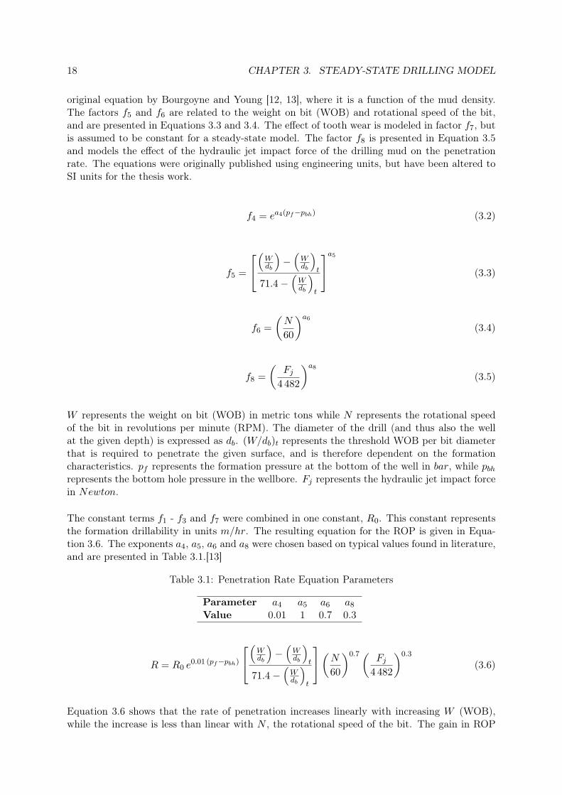
original equation by Bourgoyne and Young [12, 13], where it is a function of the mud density.The factors f5 and f6 are related to the weight on bit (WOB) and rotational speed of the bit,and are presented in Equations 3.3 and 3.4. The effect of tooth wear is modeled in factor f7, butis assumed to be constant for a steady-state model. The factor f8 is presented in Equation 3.5and models the effect of the hydraulic jet impact force of the drilling mud on the penetrationrate. The equations were originally published using engineering units, but have been altered toSI units for the thesis work.
f4 = ea4(pf−pbh) (3.2)
f5 =
(
Wdb
)−(
Wdb
)t
71.4−(
Wdb
)t
a5
(3.3)
f6 =(N
60
)a6
(3.4)
f8 =(
Fj
4 482
)a8
(3.5)
W represents the weight on bit (WOB) in metric tons while N represents the rotational speedof the bit in revolutions per minute (RPM). The diameter of the drill (and thus also the wellat the given depth) is expressed as db. (W/db)t represents the threshold WOB per bit diameterthat is required to penetrate the given surface, and is therefore dependent on the formationcharacteristics. pf represents the formation pressure at the bottom of the well in bar, while pbh
represents the bottom hole pressure in the wellbore. Fj represents the hydraulic jet impact forcein Newton.
The constant terms f1 - f3 and f7 were combined in one constant, R0. This constant representsthe formation drillability in units m/hr. The resulting equation for the ROP is given in Equa-tion 3.6. The exponents a4, a5, a6 and a8 were chosen based on typical values found in literature,and are presented in Table 3.1.[13]
Table 3.1: Penetration Rate Equation Parameters
Parameter a4 a5 a6 a8
Value 0.01 1 0.7 0.3
R = R0 e0.01 (pf−pbh)
(
Wdb
)−(
Wdb
)t
71.4−(
Wdb
)t
(N60
)0.7( Fj
4 482
)0.3
(3.6)
Equation 3.6 shows that the rate of penetration increases linearly with increasing W (WOB),while the increase is less than linear with N , the rotational speed of the bit. The gain in ROP

3.1. DRILLING MODEL EQUATIONS 19
by increased rotational speed N will be less prominent at higher values of N . Both responsesmake physical sense, though some may argue that the rate of penetration should decrease athigher values of WOB. The reason for such a physical response is widely believed to be a resultof insufficient bottom-hole cleaning, and not a direct consequence of an increase in WOB.[13]Insufficient hole cleaning will result in re-grinding of cuttings that are not quickly transportedaway from the drill bit, leading to a less-than-optimal rate of penetration. However, we assumeperfect hole cleaning conditions and expect a response similar to that of Equation 3.6.
3.1.2 Topdrive Torque and Power
The torque and power of the topdrive are useful measurement to monitor during the drillingprocess, and may be feasible variables for controlling the process. The torque that is needed torotate the drill string is the product of the force Fc and the length of the arm that the force isacting on, in this case the radius of the drill string. The force Fc can be expressed as the productof the specific cutting force kc and the area of the drilled surface, as shown in Equation 3.7,where ds denotes the diameter of the drill string.
T = Fcds
2= kc
d2b ds π
8(3.7)
The specific cutting force kc depends on the formation strength, but also on the weight on bit.It is assumed that the specific cutting force can be modeled as a product of a parameter k0
c
which only depends on the formation characteristics, multiplied with the WOB. This is shownin Equation 3.8.
kc = k0c W (3.8)
The topdrive power (in kW ) can be calculated from the torque (T ) as shown in Equation 3.9.
P =2πN T
60 000(3.9)
3.1.3 Bottom Hole Cleaning
As mentioned in Section 2.1, one of the purposes of the drilling mud is to transport the cuttingsaway from the bit and up to the surface through the well annulus. It is very important to ensuresufficient transport of the cuttings, otherwise the drill bit will keep grinding the cuttings thataccumulate at the bottom of the well. This will lead to a lower rate of penetration and thus lessefficient drilling.
The circulation rate and properties of the drilling mud determine its capacity of transportingthe cuttings. First, the slip velocity of the particles must be determined, which is dependent onthe geometry and density of the cuttings. The slip velocity for Newtonian fluids in creeping flow,i.e. very low Reynolds numbers (< 0.1), may be calculated using Stoke’s law. Choosing realisticvalues for the annulus velocity, mud density, viscosity and the diameters of the drill string andwell, an estimate of the Reynolds number may be made as shown Equation 3.11. The hydraulic

20 CHAPTER 3. STEADY-STATE DRILLING MODEL
diameter of an annulus may be calculated using Equation 3.10.
dH =π(d2
b − d2s)
π(db + ds)= db − ds (3.10)
NRe =ρf va dH
µ=
1 400 kg/m3 · 0.7m/s · (0.254m− 0.100m)0.02Pa·s
= 7 546 (3.11)
From Equation 3.11 it is clear that Stoke’s law can not be used. For Reynolds numbers over 0.1,empirically determined friction coefficients must be used. The friction coefficient in this case isdefined in Equation 3.12,
f =F
AEK(3.12)
where
• F = force exerted on the particle due to viscous drag,
• A = characteristic area of the particle, and
• EK = kinetic energy per unit volume.[13]
The force F is the difference between the weight and buoyancy of the particle, defined by Equa-tion 3.13. The particle diameter is denoted dp, while ρs and ρf denote the particle density andthe effective mud density, respectively. The kinetic energy EK is defined by Equation 3.14, wherevsl is the particle slip velocity.
F = Fg − Fbo = (ρs − ρf ) g (π d3p/6) (3.13)
EK =12ρs v
2sl (3.14)
Assuming the particles are spherical, the characteristic area is given as A = π d2p/4. Combining
the equations gives Equation 3.15 for the friction factor.
f =43gdp
v2sl
ρs − ρf
ρf(3.15)
Several correlations have been proposed in order to let the slip velocity equations apply fornon-Newtonian fluids, such as drilling muds. Moore [14, 13] proposed that for Reynolds numbersabove 300, the flow around the particle is fully turbulent and the friction factor becomes constantat a value of about 1.5. Chien [15, 13] recommends the use of 1.72 for the friction coefficient forReynolds numbers above 100. Though slightly different for lower Reynolds numbers, the differentcorrelations seems to agree rather closely for turbulent flows. Thus, using Moore’s correlationand solving Equation 3.15 for the slip velocity, we get Equation 3.16.
vsl =
√89g dp
ρs − ρf
ρf(3.16)

3.1. DRILLING MODEL EQUATIONS 21
The effective transport velocity vT of the cuttings is defined as the difference between the annulusmud velocity and the slip velocity of the particles. The expression is shown in Equation 3.17.Assuming that the mud flow through the bit (qbit) is equal to the flow of mud from the main pump(qin), the annulus flow velocity is expressed as in Equation 3.18. Aa represents the cross-sectionalarea of the well annulus.
vT = va − vslip (3.17)
va =qbitAa
=4 qin
π (d2b − d2
s)(3.18)
The transport velocity can be used to calculate the fraction of cuttings (xc) in the mud that isflowing in the well annulus, since it can also be expressed as a function of the rate of cuttings asshown in Equation 3.19.[13]
vT =qs
Aa xc(3.19)
The feed of cuttings per second (qs) is determined by the ROP (R) as shown in Equation 3.20,and the fraction of solids in the mud return can be calculated by re-organizing Equation 3.19 asshown in Equation 3.21.
qs =R
3 600Ab =
R
3 600πd2
b
4(3.20)
xc =qc
Aa vT(3.21)
The effective density of the returning mud is dependent on the fraction of cuttings, and iscalculated using Equation 3.22.
ρf = xc ρs + (1− xc) ρm (3.22)
The transport velocity vT must be greater than zero in order for the cuttings to be transportedout of the well. A negative vT means that the slip velocity is higher than the annulus velocity,resulting in an accumulation of cuttings at the bottom of the well. While a small, positive vT
in theory would bring the cuttings to the surface, this would result in a very high percentageof cuttings in the mud and significantly increase the mud density, which in turn would lead toa higher bottom-hole pressure and thus less favorable drilling conditions (refer to Equations 3.2and 3.6).
3.1.4 Bottom Hole Pressure
All measurements from the bottom of the well are in practice rather difficult to obtain. The mea-surements may be sent to the top by mud pulse telemetry, but this technology is ineffective duringtimes of lost circulation and when the mud circulation rate is low. Mud-pulse telemetry requiresa minimum flow rate of approximately 600-1000 liter/min. The measurements are updated only1-10 times per minute and experience a couple of seconds of delay as they are transmitted to
22 CHAPTER 3. STEADY-STATE DRILLING MODEL
the surface. Underbalanced drilling also imposes several other challenges to mud pulse teleme-try, as gas that is introduced to reduce the equivalent mud density causes signal attenuationand drastically reduces the ability to transmit data through the mud. However, as mentionedin Section 2.1.1, we assume we have a wired drill pipe providing accurate measurements of thebottom hole pressure.
The measurement of the bottom hole pressure was modeled using simple fluid mechanics. Theflow of mud through the well annulus to the surface may be used to determine the pressureprofile. The annulus flow is assumed to be one-dimensional and we neglect other momentumeffects that may be experienced due to the rotation of the drill string. We also assume that thedrilling fluid is incompressible.
At steady-state and applying the assumptions above, the Navier-Stokes equations are reducedto Equation 3.23. F represents the friction forces affecting the flow, z is the length coordinatealong the path of the flow (positive direction upwards), while Aa represents the cross-sectionalarea of the annulus.
0 = −∂p∂z− 1Aa
∂F
∂z− ρf g (3.23)
We assume the friction gradient ∂F/∂z is constant, and integrate Equation 3.23 from z = −Dto z = 0. D is the depth of the well in meters (D > 0). Further, we re-organize to get pbh onthe left side of the equation, and get Equation 3.24.
pbh = pc +1Aa
∂F
∂zD + ρf g D (3.24)
The friction loss term is dependent on the geometry of the flow (in this case an annulus) andis difficult to calculate accurately. For this simple model, we assume that the annulus pressuredrop due to friction is linearly dependent on the mud flow. For a mud flow of 1 m3/min, weassume a 15 bar pressure drop, giving a friction parameter θ = 15
1/60 = 900 bar · s/m3. The finalequation for the bottom-hole pressure measurement is shown in Equation 3.25.
pbh = pc + θ qin + ρf g D (3.25)
The first term represents the choke pressure, in other words the pressure at the top of theannulus. The choke pressure term is only relevant for MPD systems that involve a sealed-offannulus (RCD) and choke valve. For conventional drilling with an open mud return, pc is equal tothe atmospheric pressure. The second term represents the pressure loss due to friction. The lastterm is the hydrostatic pressure from the annulus mud column, which is the also the dominantterm in the expression.
3.2. PARAMETERS 23
3.2 Parameters
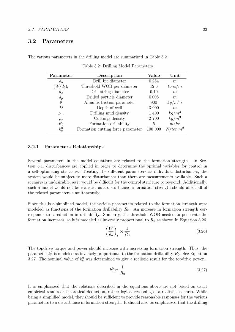
The various parameters in the drilling model are summarized in Table 3.2.
Table 3.2: Drilling Model Parameters
Parameter Description Value Unitdb Drill bit diameter 0.254 m
(W/db)t Threshold WOB per diameter 12.6 tons/mds Drill string diameter 0.10 mdp Drilled particle diameter 0.005 mθ Annulus friction parameter 900 kg/m4 sD Depth of well 3 000 mρm Drilling mud density 1 400 kg/m3
ρs Cuttings density 2 700 kg/m3
R0 Formation drillability 5 m/hrk0
c Formation cutting force parameter 100 000 N/tonm2
3.2.1 Parameters Relationships
Several parameters in the model equations are related to the formation strength. In Sec-tion 5.1, disturbances are applied in order to determine the optimal variables for control ina self-optimizing structure. Treating the different parameters as individual disturbances, thesystem would be subject to more disturbances than there are measurements available. Such ascenario is undesirable, as it would be difficult for the control structure to respond. Additionally,such a model would not be realistic, as a disturbance in formation strength should affect all ofthe related parameters simultaneously.
Since this is a simplified model, the various parameters related to the formation strength weremodeled as functions of the formation drillability R0. An increase in formation strength cor-responds to a reduction in drillability. Similarly, the threshold WOB needed to penetrate theformation increases, so it is modeled as inversely proportional to R0 as shown in Equation 3.26.(
W
db
)t
∝ 1R0
(3.26)
The topdrive torque and power should increase with increasing formation strength. Thus, theparameter k0
c is modeled as inversely proportional to the formation drillability R0. See Equation3.27. The nominal value of k0
c was determined to give a realistic result for the topdrive power.
k0c ∝
1R0
(3.27)
It is emphasized that the relations described in the equations above are not based on exactempirical results or theoretical deduction, rather logical reasoning of a realistic scenario. Whilebeing a simplified model, they should be sufficient to provide reasonable responses for the variousparameters to a disturbance in formation strength. It should also be emphasized that the drilling
24 CHAPTER 3. STEADY-STATE DRILLING MODEL
model is not based on any specific scenario or field data, but should be interpreted as a simplemodel of a fictional drilling process.
3.3 Drilling Model Results
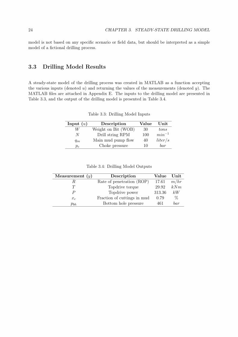
A steady-state model of the drilling process was created in MATLAB as a function acceptingthe various inputs (denoted u) and returning the values of the measurements (denoted y). TheMATLAB files are attached in Appendix E. The inputs to the drilling model are presented inTable 3.3, and the output of the drilling model is presented in Table 3.4.
Table 3.3: Drilling Model Inputs
Input (u) Description Value UnitW Weight on Bit (WOB) 30 tonsN Drill string RPM 100 min−1
qin Main mud pump flow 40 liter/spc Choke pressure 10 bar
Table 3.4: Drilling Model Outputs
Measurement (y) Description Value UnitR Rate of penetration (ROP) 17.61 m/hrT Topdrive torque 29.92 kNmP Topdrive power 313.36 kWxc Fraction of cuttings in mud 0.79 %pbh Bottom hole pressure 461 bar

Chapter 4
Optimization and Active ConstraintControl
This section will provide an analysis and overview of the various factors affecting the cost of thedrilling process in order to identify the objective function for the optimization problem. Thedegrees of freedom for optimization of the process will be presented. An equation describingthe cost of drilling (objective function) is derived, and the operational constraints will be iden-tified. Finally, the nominal optimal values of both manipulated variables and measurements aredetermined, as well as the active constraints at optimum.
4.1 Degrees of Freedom (DOF)
In general, a degree of freedom (DOF) is a single scalar number describing a micro-state of asystem. The system is then completely described by all its degrees of freedom. For processdesign, the number of steady-state DOF’s is the number of variables (parameters) that mustbe specified to completely define the process. The degrees of freedom can be calculated bysubtracting the number of specified variables (equations) from the number of process variables,as shown in Equation 4.1.
NSS = Nvar −NSV (4.1)
Nvar represents the number of process variables, and NSV represents the number of specifiedvariables (equations). However, counting equations is not a very efficient procedure. The steady-state degrees of freedom for a process may also be determined by counting the manipulatedvariables NMV and subtracting the variables with no steady-state effect and the process specifi-cations. The degrees of freedom in the drilling process involve all manipulated variables (MV’s)available to the driller. They are recapitulated in Table 4.1. We assume that Managed Pres-sure Drilling (MPD) is available, thus allowing us to use the choke pressure (pc) as a degree offreedom.
In MPD systems, the choke pressure pc is set by the choke valve and back pressure pumpassociated with the rotating control device (RCD). The choke valve is used to control the pressure,
25
26 CHAPTER 4. OPTIMIZATION AND ACTIVE CONSTRAINT CONTROL
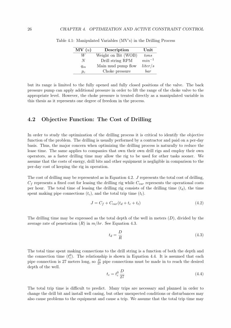
Table 4.1: Manipulated Variables (MV’s) in the Drilling Process
MV (u) Description UnitW Weight on Bit (WOB) tonsN Drill string RPM min−1
qin Main mud pump flow liter/spc Choke pressure bar
but its range is limited to the fully opened and fully closed positions of the valve. The backpressure pump can apply additional pressure in order to lift the range of the choke valve to theappropriate level. However, the choke pressure is treated directly as a manipulated variable inthis thesis as it represents one degree of freedom in the process.
4.2 Objective Function: The Cost of Drilling
In order to study the optimization of the drilling process it is critical to identify the objectivefunction of the problem. The drilling is usually performed by a contractor and paid on a per-daybasis. Thus, the major concern when optimizing the drilling process is naturally to reduce thelease time. The same applies to companies that own their own drill rigs and employ their ownoperators, as a faster drilling time may allow the rig to be used for other tasks sooner. Weassume that the costs of energy, drill bits and other equipment is negligible in comparison to theper-day cost of keeping the rig in operation.
The cost of drilling may be represented as in Equation 4.2. J represents the total cost of drilling,Cf represents a fixed cost for leasing the drilling rig while Cvar represents the operational costsper hour. The total time of leasing the drilling rig consists of the drilling time (td), the timespent making pipe connections (tc), and the total trip time (tt).
J = Cf + Cvar(td + tc + tt) (4.2)
The drilling time may be expressed as the total depth of the well in meters (D), divided by theaverage rate of penetration (R) in m/hr. See Equation 4.3.
td =D
R(4.3)
The total time spent making connections to the drill string is a function of both the depth andthe connection time (t0c). The relationship is shown in Equation 4.4. It is assumed that eachpipe connection is 27 meters long, so D
27 pipe connections must be made in to reach the desireddepth of the well.
tc = t0cD
27(4.4)
The total trip time is difficult to predict. Many trips are necessary and planned in order tochange the drill bit and install well casing, but other unexpected conditions or disturbances mayalso cause problems to the equipment and cause a trip. We assume that the total trip time may

4.2. OBJECTIVE FUNCTION: THE COST OF DRILLING 27
be expressed as a product of the time spent on a single trip multiplied by the number of trips.The number of trips required for bit changes is the drilling time (td) divided by the lifetime ofthe bit (t0d). The lifetime of the bit depends on the operating conditions and wear the bit isexposed to. In addition, a constant number of trips (1 every 1000 meters) are assumed for theinstallation of casing and other purposes. The total trip time is expressed in Equation 4.5
tt = t0t
(tdt0d
+D
1 000
)= t0t
(D
R t0d+
D
1 000
)(4.5)
Combining Equations 4.2 to 4.5, the cost function of the drilling process may be expressed asEquation 4.6.
J = Cf + Cvar
(D
R+ t0c
D
27+ t0t
(D
R t0d+
D
1 000
))(4.6)
Naturally, it is desirable to perform the drilling as fast as possible. At first glance, one mayexpect this to be ambiguous with maximizing the rate of penetration (R). However, the drill bitwear is affected by the operating conditions and is an important factor in optimizing the drilling.
4.2.1 Bit Wear
The drill bit must be changed when either the teeth or the bearings are completely worn out.[13].We assume that the bit teeth wear out before the bearings, so the bit lifetime is equivalent tothe time needed to completely wear down the teeth. According to Bourgoyne et. al. [13], thebit tooth wear may be modeled as shown in Equation 4.7
dh
dt=
1τH
(N
60
)H1
(
Wdb
)m− 71.4(
Wdb
)m−(
Wdb
)(1 +H2/2
1 +H2h
)(4.7)
where
• h = fractional tooth height that has been worn away,
• t = time, hours,
• H1, H2, (W/db)m = constants,
• τH = formation abrasiveness constant, hours.
As in Equation 3.6 on page 18, W and N represent the weight on bit and rotational speed ofthe drill string, respectively. The recommended values for H1, H2 and (W/db)m from variousrolling-cutter rock bit classes are presented in Table 4.2.[13] (W/db)m represents the maximumWOB per diameter of drill bit that should be used. For the course of this work, the drill bit hasbeen assumed to be a class 3-1 bit.
(W/db)m in Table 4.2 has units lbf/in. When converted to metric units, we get (W/db)m =178.6 tons/m. A bit diameter of 0.254 m (10 in.) gives Wm = 45.36 tons for the maximumWOB.

28 CHAPTER 4. OPTIMIZATION AND ACTIVE CONSTRAINT CONTROL
Table 4.2: Recommended Tooth-Wear Parameters for Rolling-Cutter Bits [13]
Bit Class H1 H2 (W/db)m
1-1 to 1-2 1.90 7 7.01-3 to 1-4 1.84 6 8.02-1 to 2-2 1.80 5 8.5
2-3 1.76 4 9.03-1 1.70 3 10.03-2 1.65 2 10.03-3 1.60 2 10.04-1 1.50 2 10.0
Defining a tooth wear parameter J2 as in Equation 4.8, we may rewrite Equation 4.7 as shownin Equation 4.9.
J2 =
(
Wdb
)m−(
Wdb
)(
Wdb
)m− 71.4
(60N
)H1(
11 +H2/2
)(4.8)
∫ t0d
0dt = J2τH
∫ hf
0(1 +H2h) dh (4.9)
Integrating Equation 4.9 we get Equation 4.10.
t0d = J2τH(hf +H2h2f/2) (4.10)
We assume that the same bit (class 3-1) is used consequently, so there will be no changes inparameters. By collecting the constants in one single time constant K, we get Equation 4.11.
t0d = K
(
Wdb
)m−(
Wdb
)(
Wdb
)m− 71.4
(60N
)1.7
(4.11)
K may be regarded as a bit lifetime constant and is naturally dependent on the strength andabrasiveness of the drilled formation. The bit lifetime constant K will be reduced as a resultof an increase in formation strength, and is thus modeled as proportional to the drillability R0
(Equation 4.12).K ∝ R0 (4.12)
The value of K was set to 75 hours by trial and error to give a realistic value for the bit lifetimeof approximately 15 hours.
4.2.2 Operating Modes
In addition to the operating conditions, Equation 4.6 on page 27 shows that the drilling processcosts are highly dependent on the non-drilling times (t0c and t0t ). In fact, it may be easier to divide

4.3. OPERATIONAL CONSTRAINTS 29
the process into two specific operating modes: One for the actual drilling, and one for the pipeconnections and drilling trips. This is due to the nature of the plantwide control approach of thisproject. The same objectives are not applicable to bothmodes of the process. During connectionsand trips, pressure control is the only relevant control objective. The design and performance ofthe pressure control system during pipe connections and trips is studied in Chapter 6.
During the actual drilling operation, the specific connection time (t0c) and trip time (t0t ) may beassumed constant. Thus, the second term in the main brackets of Equation 4.6 and the last termregarding the trip time are regarded as constant. With respect to minimizing the cost function,constant terms are irrelevant and may be neglected. The resulting equation is presented inEquation 4.13.
min J = min(D
R+ t0t
D
R t0d
)(4.13)
The trip time constant t0t was assumed to be 10 hours. The other terms (penetration rate Rand the bit-lifetime t0d) are dependent on the drilling operating conditions and are part of theoptimization problem. The total well depth D is constant and could be removed, but was keptin the objective function in order to give it the more comprehensible units of time (hours). Thedepth D was set to 3 000 meters.
4.3 Operational Constraints
There are several constraints that need to be taken into account during drilling, both for measure-ments and for inputs. The most important constraints are the pressure constraints, as describedin Section 2.1.1. The bottom hole pressure must be controlled within its limits very accurately.We assume the bottom hole pressure is constrained between 470 and 480 bar for a depth of 3 000meters.
The weight on bit (WOB) is constrained by the threshold WOB (Table 3.2) on page 23 and themaximum WOB per diameter (W/db)m (Table 4.2 on page 28). We assume that the rotationalspeed of the drill string has an upper constraint of 200 RPM, as values above this would mostlikely cause problems for the equipment. The specifications of the topdrive motor naturallyprovide physical limits for the torque and power. However, we assume that the topdrive hassufficient capacity to operate at the optimal conditions.
The mud circulation rate may be altered in order to affect various measurements, such as thepressure profile, the fraction of cuttings in the returning mud, or the penetration rate. A highmud circulation rate will provide a higher jet impact force through the nozzles of the drillbit. However, increasing the mud flow rate beyond a certain point will eventually increase thefrictional losses in both drill string and annulus. In turn, this will reduce the jet impact force atthe bit, thus reducing the rate of penetration and increasing the drilling costs.[13] A high mudcirculation rate also increases the risk of mud loss if the well is overbalanced. In order to takethese considerations into account in the optimization problem, the mud flow rate was constrainedat a maximum of 50 liter/s. The operational constraints are recapitulated in Table 4.3.

30 CHAPTER 4. OPTIMIZATION AND ACTIVE CONSTRAINT CONTROL
Table 4.3: Operational Constraints in the Drilling Process
Constraint Lower Bound Upper Bound UnitW 3.2 45.4 tonsN 0 200 min−1
qin 0 50 liter/spbh 470 480 bar
4.4 Optimization Results
The optimization of the drilling process was carried out in MATLAB using the fmincon functionfor non-linear constrained minimization. The active-set algorithm for the fmincon function usesa sequential quadratic programming (SQP) method, solving a quadratic program (QP) at eachiteration and updating an estimate of the Hessian of the Lagrangian function.[16]
The scripts and functions that were used are attached in Appendix E. The nominal optimalvalues for the objective function, the manipulated variables and the measurements are presentedin Table 4.4. Some information about the optimization routine is presented in Table 4.5.
Table 4.4: Nominal Optimal Values
Obj. fun. Nom. opt. UnitJ 249.09 hours
MV’s Nom. opt. UnitW 33.1 tonsN 100 min−1
qin 50 liter/spc 10.3 bar
Measurements Nom. opt. UnitR 20.5 m/hrT 33 kNmP 344 kWxc 0.7 %pbh 470.0 bar
Table 4.5: Details About the Optimization
Number of iterations 24Function Evaluations 131
First order optimality measure 3.8 · 10−4
Active inequalities 2

4.5. ACTIVE CONSTRAINTS 31
The Hessian of the Lagrangian function (refer to Section 2.2) at optimum is presented below.
∇2uuL(u, λ) = 104 ·
0.1005 −0.0006 −0.1483 0.5960−0.0006 0.0086 0.0063 −0.0218−0.1483 0.0063 0.2223 −0.89080.5960 −0.0218 −0.8908 3.5719
The active constraints in the optimization are the lower bottom hole pressure constraint and theupper mud circulation rate constraint.
4.5 Active Constraints
It is important to control the constraints that are active at the optimum to ensure optimaloperation. This holds for any type of process. As an example, consider a chemical plant producingproduct A that is sold with a purity requirement of 95%. The purity specification constraint willlikely be active at optimal operation, because it is uneconomic to produce the product with ahigher purity. A purity that is higher than the required specification would mean the company isselling a higher value product for a lesser price. In order to ensure optimal operation of the plantwhen disturbances to the process occur, it is important to control the purity by a manipulatedvariable (e.g. heat applied to separation process, or feed of a specific reactant).
The active constraints in the drilling process model are the bottom hole pressure (pbh) and themud circulation rate (qin). The control of each active constraint consumes one manipulatedvariable (MV). We assume the bottom hole pressure is controlled using the choke pressure (pc)as described in Section 2.1.1, and thus omit the choke pressure and the mud flow rate fromfurther analysis.
4.6 Unconstrained Optimization
The bottom hole pressure and the mud circulation rate are omitted from the optimization, andare specified at their constrained values shown in Table 4.6.
Table 4.6: Active Constraints in the Drilling Process
Active Constraint Value Unitqin 50 liter/spbh 470 bar
The remaining optimization problem is unconstrained. The Hessian matrix of the objectivefunction (Juu) at the unconstrained optimum is presented below.
∇2J(u) = Juu =[1.8816 0.11590.1159 0.0222
]

32 CHAPTER 4. OPTIMIZATION AND ACTIVE CONSTRAINT CONTROL
Graphical representations of the objective function versus the two unconstrained degrees offreedom, the weight on bit (WOB) and rotational speed of the drill string, are presented inFigures 4.1a and 4.1b. A 3-dimensional surface plot of the objective function is presented inFigure 4.2.
(a) J(u,d) vs. WOB (N = 150 rpm) (b) J(u,d) vs. RPM (WOB = 25 tons)
Figure 4.1: Plots of the objective function J(u, d) vs the weight on bit (WOB) and the drillstring RPM.
Figure 4.2: Surface plot of the objective function J(u, d) versus the WOB and the drill stringRPM.
The remaining task is to determine what variables should be controlled by the two unconstraineddegrees of freedom in the drilling process. The choices of controlled variables may give verydifferent results when the drilling process is subject to disturbances. This will be analyzed inChapter 5.

Chapter 5
Self-Optimizing Controlled Variables
This section will cover the process of selecting the variables that should be controlled during thedrilling process. The theory was described in detail in Section 2.3.
The results of Chapter 4 showed that two degrees of freedom must be used to control the activeconstraints. Assuming the MPD system with the choke and backpressure pump is used to controlthe bottomhole pressure and the mud circulation rate is kept at its constrained value, we are leftwith two manipulated variables:
• Weight on Bit (W )
• Drill string rotary speed (N)
The manipulated variables can be used to control various measurements in order to gain moreprofitable operation when the drilling process is subject to disturbances.
The best controlled variables may be identified by a brute-force evaluation, implementing con-trol of various combinations of controlled variables, introducing the expected disturbances andcalculating the loss compared to the re-optimized value of the objective function. While theprocess only involves two unconstrained degrees of freedom and thus two controlled variables leftto determine, a brute-force evaluation is rather tedious work. We have six variables availableafter removing the bottom hole pressure, choke pressure and mud flow rate from the analysis.Therefore, we are left with 6!
2! 4! =(62
)= 15 combinations of controlled variables. It is important
to recognize that the manipulated variables are treated as measurements when determining thecontrolled variables. In case a manipulated variable is used as a controlled variable, it meansthat it is beneficial to keep the MV constant.
Instead of performing a brute-force evaluation, we may determine the self-optimizing controlledvariables by various mathematical methods. The procedures and results of the maximum scaledgain (minimum singular value) method, the null space method and the exact local method aredescribed in Sections 5.2, 5.3 and 5.4.
33

34 CHAPTER 5. SELF-OPTIMIZING CONTROLLED VARIABLES
5.1 Process Gains and Disturbances
The process gains from the inputs to the measurements (outputs) can be achieved by applyingsmall perturbations to the manipulated variables. The magnitude of the perturbations was 1% ofthe nominal value. The calculation is performed as shown in Equation 5.1, and the gain matrixis presented in Appendix B. The MATLAB script is presented in Appendix E. The inputsthemselves are included as the bottom two measurements in the gain matrix, so the bottom 2×2matrix is naturally an identity matrix.
Gi,j =∆yi
∆uj=yi − y0
i
uj − u0j
(5.1)
The first steps in selecting the optimal controlled variables is identifying the sensitivity of themeasurements to various disturbances. As described in Section 3.2.1, the parameters relatedto the formation strength were all modeled to be functions of the drillability parameter R0.In addition to the formation strength, disturbances in the formation density and the bottomhole pressure were introduced. The disturbance parameters were perturbed 1%, and the drillingprocess was re-optimized after each disturbance in order to determine the optimal variation ofthe process variables. The disturbance sensitivity matrix F was calculated using Equation 5.2,and is presented below. The left column of F represents the disturbance in formation drillability(R0), the middle column represents the disturbance in formation density (ρs), while the rightmostcolumn represents the disturbance in the bottom hole pressure (pbh).
Fi,j =∆yi,opt
∆dj=yi,opt − y0
i,opt
dj − d0j
(5.2)
F =
3.94 0.00 −0.15−6.71 −0.00 −0.00−27.05 0.00 0.00
0.26 0.00 −0.01−0.18 −0.00 −0.0012.60 0.00 0.00
The expected magnitudes the disturbances are presented in Table 5.1.
Table 5.1: Expected Disturbances
Disturbance Magnitude UnitR0 -2.5 m/hrρs 500 kg/m3
pbh 10 bar
The expected implementation errors (n) for each measurement (y) were estimated based onassumptions of measurement sensitivity, and are presented in Table 5.2.
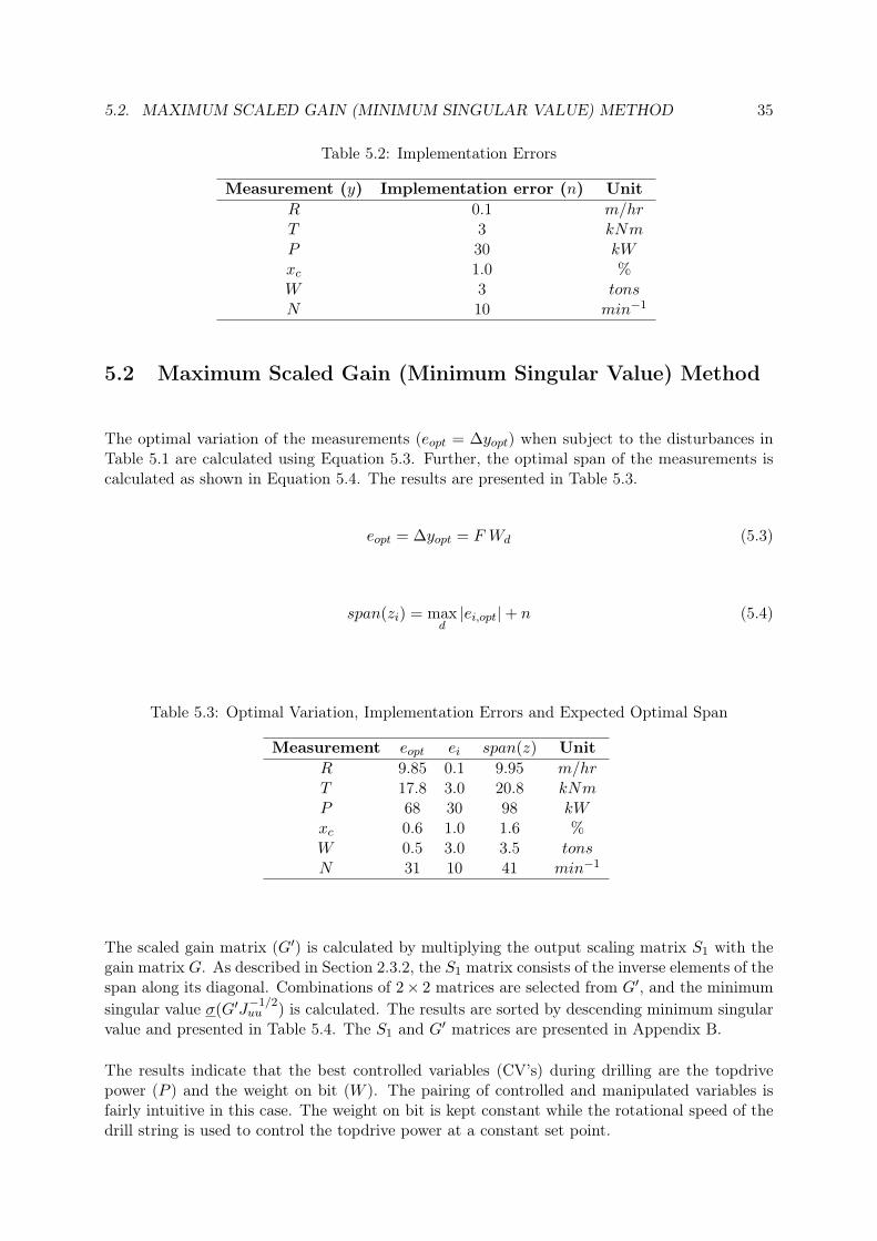
5.2. MAXIMUM SCALED GAIN (MINIMUM SINGULAR VALUE) METHOD 35
Table 5.2: Implementation Errors
Measurement (y) Implementation error (n) UnitR 0.1 m/hrT 3 kNmP 30 kWxc 1.0 %W 3 tonsN 10 min−1
5.2 Maximum Scaled Gain (Minimum Singular Value) Method
The optimal variation of the measurements (eopt = ∆yopt) when subject to the disturbances inTable 5.1 are calculated using Equation 5.3. Further, the optimal span of the measurements iscalculated as shown in Equation 5.4. The results are presented in Table 5.3.
eopt = ∆yopt = F Wd (5.3)
span(zi) = maxd|ei,opt|+ n (5.4)
Table 5.3: Optimal Variation, Implementation Errors and Expected Optimal Span
Measurement eopt ei span(z) UnitR 9.85 0.1 9.95 m/hrT 17.8 3.0 20.8 kNmP 68 30 98 kWxc 0.6 1.0 1.6 %W 0.5 3.0 3.5 tonsN 31 10 41 min−1
The scaled gain matrix (G′) is calculated by multiplying the output scaling matrix S1 with thegain matrix G. As described in Section 2.3.2, the S1 matrix consists of the inverse elements of thespan along its diagonal. Combinations of 2× 2 matrices are selected from G′, and the minimumsingular value σ(G′J−1/2
uu ) is calculated. The results are sorted by descending minimum singularvalue and presented in Table 5.4. The S1 and G′ matrices are presented in Appendix B.
The results indicate that the best controlled variables (CV’s) during drilling are the topdrivepower (P ) and the weight on bit (W ). The pairing of controlled and manipulated variables isfairly intuitive in this case. The weight on bit is kept constant while the rotational speed of thedrill string is used to control the topdrive power at a constant set point.

36 CHAPTER 5. SELF-OPTIMIZING CONTROLLED VARIABLES
Table 5.4: Minimum Singular Value Results
z1 z2 σ(G′J−1/2uu )
P W 0.243W N 0.159R W 0.077P N 0.058R T 0.051T P 0.050T N 0.043R N 0.042xc W 0.037T xc 0.037R P 0.018xc N 0.021P xc 0.009R xc 0.0000T W 0.0000
5.3 Null Space Method
We have two manipulated variables and three disturbances. However, we assume that the dis-turbance in drillability R0 is the most prevalent and thus neglect the other disturbances. Theassumption is supported by analyzing the disturbance sensitivity matrix F . The sensitivities toa disturbance in R0 (the leftmost column) are much higher than the other disturbances.
Thus, we consider only one disturbance and choose ny = nu + nd = 2 + 1 = 3 measurements tocombine in order to calculate the optimal measurement combination using the null space method.It should not matter which measurements are selected. However, we analyze the disturbancesensitivity matrix F and pick measurements with smallest relative sensitivity. Thus, we chooseto combine the measurements of the topdrive power (P ), the weight on bit (W ) and the drillstring rotational speed (N).
The left null space of the new disturbance sensitivity matrix F (containing only the rowscorresponding to P , W and N) was calculated, giving the measurement combination matrix(Hnullspace) below. The results were normalized so the Euclidean norm of each row in H wasequal to unity.
Hnullspace =[−0.01 1.00 0.000.42 0.00 0.91
]
The first row of Hnullspace is approximately equal to controlling the weight on bit (W ), while thesecond row indicates controlling a combination of the topdrive power (P ) and the drill stringRPM. Therefore, the results do not differ too much from those obtained using the method ofmaximizing the singular value. However, the nullspace method does not take implementationerrors into account, and is therefore not the most reliable method for determining self-optimizingcontrol variables.

5.4. EXACT LOCAL METHOD 37
5.4 Exact Local Method
We use the exact local method to determine the optimal measurement combinations for thecontrolled variables, this time considering the effects of implementation errors. The F matrix isconstructed as shown below:
F =[F Wd Wn
]Using the exact local method, we may choose how many measurements we wish to combine inour controlled variables. The loss is reduced by increasing the number of measurements thatare combined, but this also increases the complexity of the controller. In order to achieve theoptimal measurement combination matrices H, we solve the optimization problem presented inEquation 5.5.
minH||HF ||2 (5.5)
subject to: HG = J1/2uu
The exact local method was solved by vectorizing the appropriate matrices and solving a quadraticminimization problem subject to linear constraints. The procedures are shown in Appendix C.The optimal measurement combinations and the corresponding maximum losses are presentedin Table 5.5. The complete tables with all the results of the exact local method are presented inTables D.1 to D.5 in Appendix D. The rows of the measurement combination matrices H werenormalized so the Euclidean norm of each row was equal to unity. The normalization shouldmake it easier to interpret the effect of each individual measurement to the controlled variable.
The number of measurements that are combined the controlled variables declines as the tableextends downward. The last row represents no control, thus keeping the inputs (WOB anddrill string RPM) constant. When only two measurements are combined, the measurementcombination matrix H is irrelevant and single measurements can be chosen instead. This canbe seen from Equation 5.6. If H is a square matrix we get HH−1 = I, and it is clear that thechoice of H has no effect on the loss.
L =12||J1/2
uu (HG)−1HF ||22 (5.6)
The loss decreases as we increase the number of measurements that are combined. This isexpected, as the effect of the optimal variation of each measurement is reduced by combining anincreasing amount of measurements. A graphical representation of the losses plottet against thenumber of measurements is presented in Figure 5.1.
The losses in Table 5.5 are the maximum losses, in other words the loss when the magnitude of theexpected disturbances (d′) and implementation errors (n′) is unity. Figure 5.2 shows a graphicalrepresentation of the loss function for the six candidate optimal measurement combinations(presented in Table 5.5) as a function of the magnitude of the disturbances and implementationerrors. The results show that the loss using a constant input policy is less than six hours higherthan the optimal combination of two measurements (P and W ).
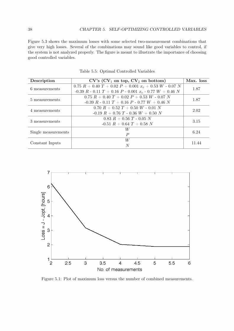
38 CHAPTER 5. SELF-OPTIMIZING CONTROLLED VARIABLES
Figure 5.3 shows the maximum losses with some selected two-measurement combinations thatgive very high losses. Several of the combinations may sound like good variables to control, ifthe system is not analyzed properly. The figure is meant to illustrate the importance of choosinggood controlled variables.
Table 5.5: Optimal Controlled Variables
Description CV’s (CV1 on top, CV2 on bottom) Max. loss
6 measurements 0.75 R + 0.40 T + 0.02 P + 0.001 xc + 0.53 W - 0.07 N 1.87-0.39 R - 0.11 T + 0.16 P - 0.001 xc - 0.77 W + 0.46 N
5 measurements 0.75 R + 0.40 T + 0.02 P + 0.53 W - 0.07 N 1.87-0.39 R - 0.11 T + 0.16 P - 0.77 W + 0.46 N
4 measurements 0.70 R + 0.52 T + 0.50 W - 0.01 N 2.02-0.19 R + 0.76 T - 0.36 W + 0.50 N
3 measurements 0.83 R + 0.56 T - 0.05 N 3.15-0.51 R + 0.64 T + 0.58 N
Single measurements W 6.24P
Constant Inputs W 11.44N
Figure 5.1: Plot of maximum loss versus the number of combined measurements.
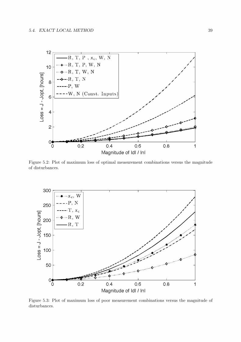
5.4. EXACT LOCAL METHOD 39
Figure 5.2: Plot of maximum loss of optimal measurement combinations versus the magnitudeof disturbances.
Figure 5.3: Plot of maximum loss of poor measurement combinations versus the magnitude ofdisturbances.
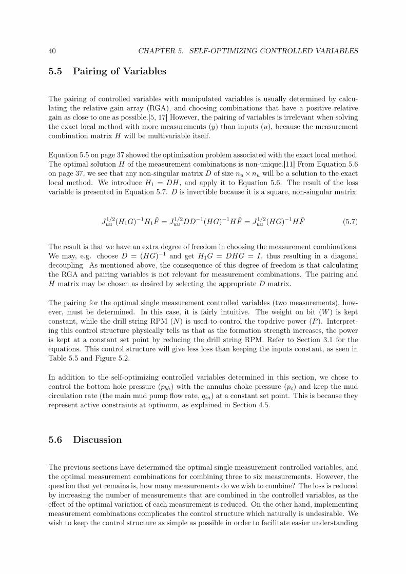
40 CHAPTER 5. SELF-OPTIMIZING CONTROLLED VARIABLES
5.5 Pairing of Variables
The pairing of controlled variables with manipulated variables is usually determined by calcu-lating the relative gain array (RGA), and choosing combinations that have a positive relativegain as close to one as possible.[5, 17] However, the pairing of variables is irrelevant when solvingthe exact local method with more measurements (y) than inputs (u), because the measurementcombination matrix H will be multivariable itself.
Equation 5.5 on page 37 showed the optimization problem associated with the exact local method.The optimal solution H of the measurement combinations is non-unique.[11] From Equation 5.6on page 37, we see that any non-singular matrix D of size nu×nu will be a solution to the exactlocal method. We introduce H1 = DH, and apply it to Equation 5.6. The result of the lossvariable is presented in Equation 5.7. D is invertible because it is a square, non-singular matrix.
J1/2uu (H1G)−1H1F = J1/2
uu DD−1(HG)−1HF = J1/2
uu (HG)−1HF (5.7)
The result is that we have an extra degree of freedom in choosing the measurement combinations.We may, e.g. choose D = (HG)−1 and get H1G = DHG = I, thus resulting in a diagonaldecoupling. As mentioned above, the consequence of this degree of freedom is that calculatingthe RGA and pairing variables is not relevant for measurement combinations. The pairing andH matrix may be chosen as desired by selecting the appropriate D matrix.
The pairing for the optimal single measurement controlled variables (two measurements), how-ever, must be determined. In this case, it is fairly intuitive. The weight on bit (W ) is keptconstant, while the drill string RPM (N) is used to control the topdrive power (P ). Interpret-ing this control structure physically tells us that as the formation strength increases, the poweris kept at a constant set point by reducing the drill string RPM. Refer to Section 3.1 for theequations. This control structure will give less loss than keeping the inputs constant, as seen inTable 5.5 and Figure 5.2.
In addition to the self-optimizing controlled variables determined in this section, we chose tocontrol the bottom hole pressure (pbh) with the annulus choke pressure (pc) and keep the mudcirculation rate (the main mud pump flow rate, qin) at a constant set point. This is because theyrepresent active constraints at optimum, as explained in Section 4.5.
5.6 Discussion
The previous sections have determined the optimal single measurement controlled variables, andthe optimal measurement combinations for combining three to six measurements. However, thequestion that yet remains is, how many measurements do we wish to combine? The loss is reducedby increasing the number of measurements that are combined in the controlled variables, as theeffect of the optimal variation of each measurement is reduced. On the other hand, implementingmeasurement combinations complicates the control structure which naturally is undesirable. Wewish to keep the control structure as simple as possible in order to facilitate easier understanding

5.6. DISCUSSION 41
of the controllers and also ease the tuning.
The graphical representation of the loss versus the number of measurements in Figure 5.1 showsus that the reduction in loss from combining more than four measurements is negligible. Thus,we should not worry about using more than four measurements in the controlled variables. Thenext question is whether we want to choose single measurements for the controlled variables, orwhether we want the lower loss, but increased complexity, of introducing measurement combi-nations. In the case of measurement combinations being chosen, one might as well combine fourmeasurements instead of three. The difference in controller design is minimal, but the reductionin loss is more prominent (see Figure 5.1).
The last option available is not selecting any controlled variables for the two unconstraineddegrees of freedom, thus keeping them at constant values. The expected loss with such a constantinput policy was shown in Figure 5.2. The loss is less than 12 hours of a total active drillingtime of approximately 550 hours. The time spent making pipe connections and drilling trips,as well as the non-productive time is not included in the active drilling time. Thus, the losswith constant inputs is 2.2% of the active drilling time. The loss when controlling the optimalcombination of four measurements is 2 hours. This means that the savings with a measurementcombination control structure are approximately 10 hours, or 1.8% of the active drilling time.Similar results have been reported in drilling literature by Reed [18] and Galle and Woods [19].Reed [18] indicated a difference of less than 3% between constant and variable bit weight androtary speed for the cases studied, while Galle and Woods [19] reported that the costs were onlyslightly higher with constant inputs.
The optimal controlled variables using single measurements are the topdrive power and theweight on bit. This control structure gives a loss of approximately 6 hours. Thus, the savingscompared to a constant input policy are less than 6 hours, or 1.1% of the active drilling time.
The drilling process is subject to much uncertainty regarding unforeseen events and accidents suchas stuck pipe, drilling kicks and equipment failure. These incidents necessitate non-productivetime on the drill rig, which is just as costly as the time spent drilling. According to Godhavn[20], the non-productive time may count up to 30% of the total drilling time. Compared tonon-productive times of such magnitudes, savings of 1-2% in active drilling time seem negligible.However, the per-day rate of drilling is very costly, and any time saved equals a substantialrevenue.
Another possibility is to discard the constant set point policy and control of self-optimizingcontrolled variables, and rather install a real-time optimizer (RTO). Eren and Ozbayoglu [21]suggest that real-time optimizers will be widely used in future drilling activities. A RTO ishierarchically positioned above the control layer (see Figure 2.2 on page 10), and continuouslyoptimizes the drilling process for the process parameters at the given time. The RTO unit thenpasses the optimal values of the process variables as set points to the control layer, as illustratedin Figure 2.4 on page 13. However, installing a RTO requires an on-line computer databasewith a continuous feed of accurate drilling parameters. Real-time optimization may not be asreliable as operating with constant set points, and may prove to involve more effort than isreflected in the outcome. The loss with a constant set point policy for a optimal combination ofmeasurements very small relative to the total drilling time. It may be likely that the increasedsavings of installing an RTO are not worth the increased complexity of the control structure.

42 CHAPTER 5. SELF-OPTIMIZING CONTROLLED VARIABLES
5.7 Stick-Slip Phenomenon
The drill string is a long, relatively thin-walled metal pipe extending several thousand meters.It is natural that the drill string experiences vibrations during drilling. The vibrations areclassified as torsional, axial and lateral vibrations, each presenting a challenge to the drillingprocess. Torsional vibrations may result in stick-slip oscillations of the drill string, while axialvibrations may cause the drill string to oscillate along its vertical axis, thus making the bitbounce against the bottom of the well. Lateral vibrations may cause the drill bit to rotatearound multiple centers in the borehole in a whirling fashion, thus drilling an oversized hole andreducing the rate of penetration. The stick-slip phenomenon is in particular considered to be amajor problem in drilling operations, and has been frequently addressed in drilling literature.
Torsional vibrations in the drill string and the stick-slip phenomenon arise from the differencebetween static and dynamic friction. Various downhole conditions such as drag, doglegs (bends),tight hole sections or formation characteristics may cause the bit to temporarily get stuck or stallin the formation while the topdrive continues to rotate the drill string. The result is that torsionalenergy is built up in the drill string until the energy overcomes the static friction between the drillbit and the formation. Since the dynamic friction is lower than the static friction, the drill stringhas excessive energy stored up to propel itself around. The result is that once the bit comes loose,it rotates or whips around at a very high speed. This creates a torsional wave that travels up thedrill string to the surface and the topdrive. If the topdrive is operated at a constant speed, it willact as a fixed end to the drill string and reflect the torsional wave back down. When reachingthe bit, the torsional wave may cause it to stall again, thus repeating the stick-slip cycle. Thestick-slip motion causes fatigue to the drill string, specially at the pipe connection joints, andcauses severe axial and lateral vibrations during the slip phase. The consequences are excessivebit wear and a reduced rate of penetration.[22, 23]
The stick-slip phenomenon can be encountered even without the effect of physical conditions suchas described above. At low rotational speeds, the transition between static and dynamic frictioncauses a drop in the frictional torque, as shown in Figure 5.4.[22, 24, 25] The negative slopeof the friction torque with respect to the rotational speed has an anti-damping effect, causingthe magnitude of the stick-slip phenomenon to increase with each cycle. Thus, when operatingwith a drill string rotational speed in the transition phase, the drill string will experience self-sustained stick-slip oscillations. Increasing the rotational speed above the critical speed willcause the oscillations to be dampened and thus eventually reach a constant value. However, theoptimal rotary speed may be lower than the critical speed for torsional oscillations. Therefore, itis desirable to be able to operate in this region without experiencing the stick-slip phenomenon.
Several solutions to eliminate stick-slip have been presented in drilling literature, such as soft-torque systems, manipulating the weight on bit (WOB) or introducing a vibration damper in thebottom hole assembly (BHA).[22] The solution involving the use a torque feedback control systemwith a varying drill string rotational speed seems to be most widespread.[26, 27] In conventionaldrilling, the topdrive is designed to keep the rotational speed of the drill string at a constantvalue. As described above, such a system will reflect the torsional wave and introduce stick-sliposcillations if operated below the critical RPM. Instead, Halsey et. al. [26] proposed lettingthe topdrive respond to the dynamic torque oscillations in such a way that the vibrations aredampened or absorbed. The control system involved implementing torque measurement at thedrilling floor and controlling the torque by manipulating the rotational speed of the drill string.

5.7. STICK-SLIP PHENOMENON 43
Figure 5.4: Plot of friction torque as a function of rotational speed of the drill string.[25]
The torque feedback control system was studied further by Javanmardi et. al. [27], implementinga direct measurement of the torque from the topdrive motor current and voltage measurements.The system was tested on off-shore wells with significant reductions on torque fluctuations andstick-slip conditions. In addition, the performance of the torque feedback control system wasfound to increase when reducing the inertia of the topdrive.[28]
The problems regarding the stick-slip phenomenon seem to be closely related to keeping a con-stant drill string rotational speed. Applying the results from the drilling literature that weredescribed above, we may assume that a constant input (WOB and drill string RPM) controlstructure could potentially be subject to stick-slip conditions and thus give non-optimal drillingoperation. On the other hand, using the drill string rotational speed to control the topdrivepower, or other combinations of measurements, implies a varying rotary speed input. Distur-bances in lithology that may provoke stick-slip will be compensated by the rotational speed ofthe drill string in order to keep the controlled variable at its set point. Thus, it is likely thatvarying the drill string RPM will reduce the reflection of torsional vibrations from the topdriveand thus dampen stick-slip oscillations in a similar manner as the torque feedback systems ofHalsey et. al. [26] and Javanmardi et. al. [27].
Other solutions to avoid stick-slip conditions involve increasing the rotational speed above thecritical value. However, an excessive drill string RPM may lead to lateral vibrations, that againreduce the rate of penetration.[22] Additionally, merely changing an input from its optimal valuewill result in non-optimal operating conditions. The increase in drill string RPM may however becompensated (or even completely substituted) by reducing the weight on bit, since the torque isdependent on the WOB. The structure of such a control system is quite sophisticated. Therefore,an alternative solution to avoiding stick-slip could be implemented in a supervisory control layer(refer to Figure 2.2 on page 10), involving a model predictive controller (MPC). Recognizingstick-slip conditions, the MPC could optimize the process (avoiding stick-slip) and determinenew optimal set points for the weight on bit and drill string rotational speed.

44 CHAPTER 5. SELF-OPTIMIZING CONTROLLED VARIABLES
Chapter 6
Pressure Control and Automation
Although it is important to drill fast and efficiently, the efficiency during non-drilling operationssuch as pipe connections and trips is equally important to optimize the total drilling process.These operations make up a significant portion of the total time, as explained in Section 4.2.
During the entire drilling process, it is important to accurately control the pressure profile ofthe well in order to prevent unwanted influx of reservoir fluids or outflux (loss) of mud into theformation. This is a challenging task, as the procedures during pipe connections and drilling tripshave a large impact on the pressure. Since the main pump is disconnected for each connection,the mud circulation is stopped and the pressure term due to friction is lost (refer to Section 3.1).Similarly, full retraction of the drill string (trip) increases the volume of the well and lowers theheight of the mud column, leading to a loss of hydrostatic pressure. Using MPD technology,these disturbances can be compensated for using the choke valve and back pressure pump tocontrol the bottom hole pressure as explained in Section 2.1.1.
The performance of the pressure control system is essential to the speed of these operations.Referring to Equation 4.6 on page 27, minimizing t0c and t0t will minimize the total drilling timeand costs. However, it is important to realize that these operations are independent from theactual drilling tasks. During connections and trips, pressure control and the speed of operationsare the only relevant control objectives.
During a pipe connection or trip, the task of ramping down the main pump while simultaneouslyramping up the back pressure pump and keeping the bottom hole pressure within its marginsis a challenging tasks for the drillers. It would be highly beneficial to design an automatedprocedure and control system for each pipe connection process, as well as trips. Ideally, theoperator would only need to initiate e.g. a pipe connection program and the required procedureswould be handled automatically by the drilling control system.
45
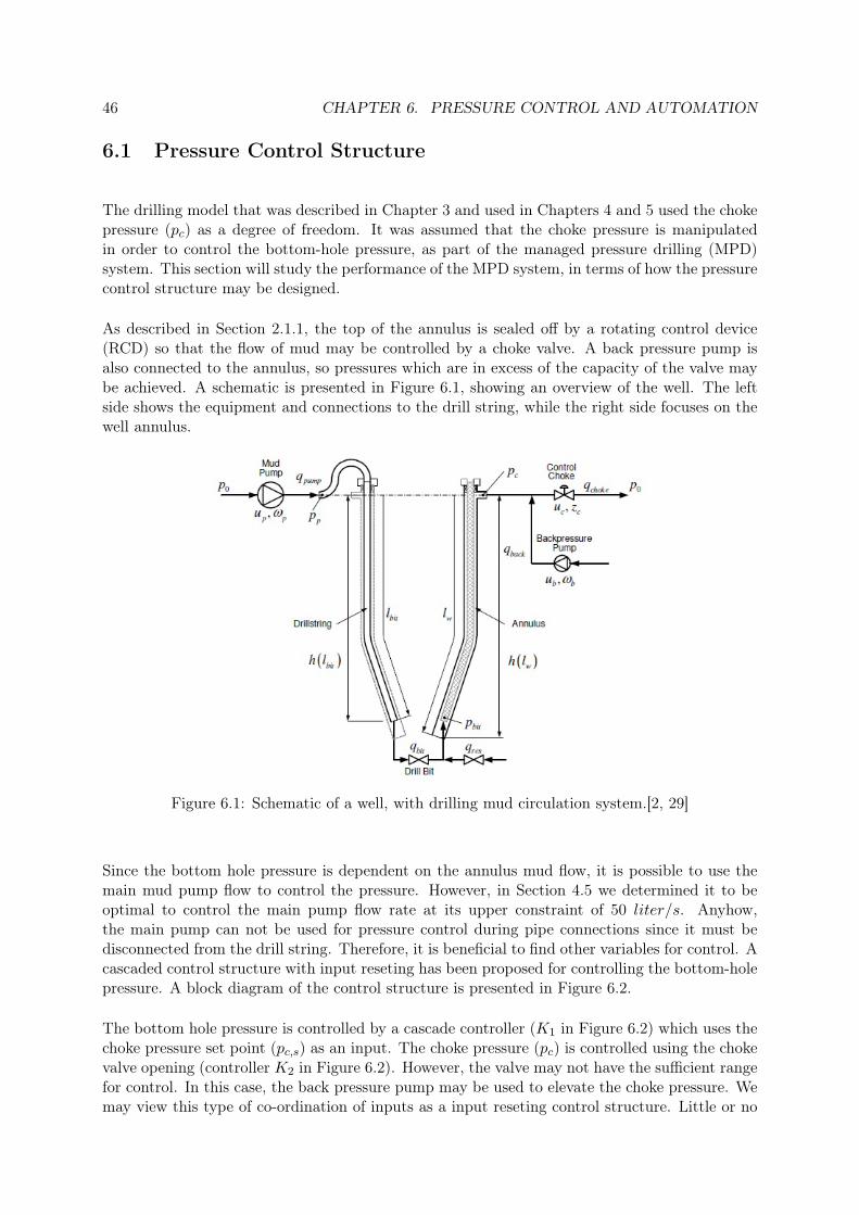
46 CHAPTER 6. PRESSURE CONTROL AND AUTOMATION
6.1 Pressure Control Structure
The drilling model that was described in Chapter 3 and used in Chapters 4 and 5 used the chokepressure (pc) as a degree of freedom. It was assumed that the choke pressure is manipulatedin order to control the bottom-hole pressure, as part of the managed pressure drilling (MPD)system. This section will study the performance of the MPD system, in terms of how the pressurecontrol structure may be designed.
As described in Section 2.1.1, the top of the annulus is sealed off by a rotating control device(RCD) so that the flow of mud may be controlled by a choke valve. A back pressure pump isalso connected to the annulus, so pressures which are in excess of the capacity of the valve maybe achieved. A schematic is presented in Figure 6.1, showing an overview of the well. The leftside shows the equipment and connections to the drill string, while the right side focuses on thewell annulus.
Figure 6.1: Schematic of a well, with drilling mud circulation system.[2, 29]
Since the bottom hole pressure is dependent on the annulus mud flow, it is possible to use themain mud pump flow to control the pressure. However, in Section 4.5 we determined it to beoptimal to control the main pump flow rate at its upper constraint of 50 liter/s. Anyhow,the main pump can not be used for pressure control during pipe connections since it must bedisconnected from the drill string. Therefore, it is beneficial to find other variables for control. Acascaded control structure with input reseting has been proposed for controlling the bottom-holepressure. A block diagram of the control structure is presented in Figure 6.2.
The bottom hole pressure is controlled by a cascade controller (K1 in Figure 6.2) which uses thechoke pressure set point (pc,s) as an input. The choke pressure (pc) is controlled using the chokevalve opening (controller K2 in Figure 6.2). However, the valve may not have the sufficient rangefor control. In this case, the back pressure pump may be used to elevate the choke pressure. Wemay view this type of co-ordination of inputs as a input reseting control structure. Little or no
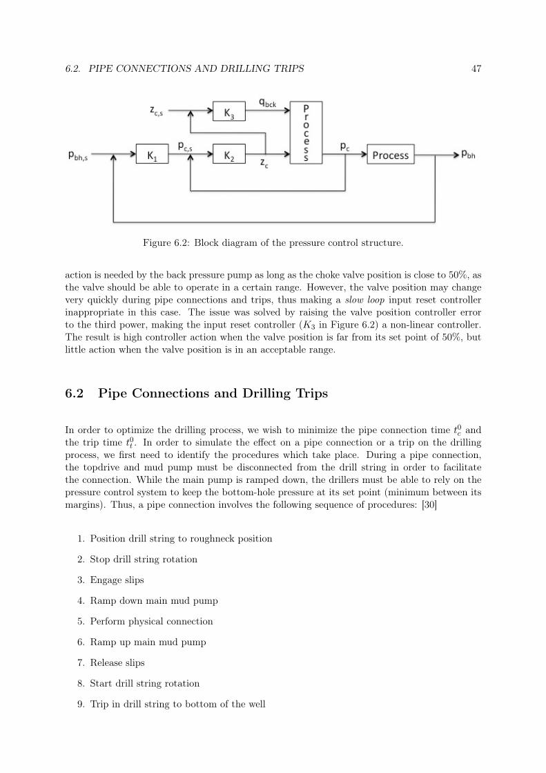
6.2. PIPE CONNECTIONS AND DRILLING TRIPS 47
Figure 6.2: Block diagram of the pressure control structure.
action is needed by the back pressure pump as long as the choke valve position is close to 50%, asthe valve should be able to operate in a certain range. However, the valve position may changevery quickly during pipe connections and trips, thus making a slow loop input reset controllerinappropriate in this case. The issue was solved by raising the valve position controller errorto the third power, making the input reset controller (K3 in Figure 6.2) a non-linear controller.The result is high controller action when the valve position is far from its set point of 50%, butlittle action when the valve position is in an acceptable range.
6.2 Pipe Connections and Drilling Trips
In order to optimize the drilling process, we wish to minimize the pipe connection time t0c andthe trip time t0t . In order to simulate the effect on a pipe connection or a trip on the drillingprocess, we first need to identify the procedures which take place. During a pipe connection,the topdrive and mud pump must be disconnected from the drill string in order to facilitatethe connection. While the main pump is ramped down, the drillers must be able to rely on thepressure control system to keep the bottom-hole pressure at its set point (minimum between itsmargins). Thus, a pipe connection involves the following sequence of procedures: [30]
1. Position drill string to roughneck position
2. Stop drill string rotation
3. Engage slips
4. Ramp down main mud pump
5. Perform physical connection
6. Ramp up main mud pump
7. Release slips
8. Start drill string rotation
9. Trip in drill string to bottom of the well

48 CHAPTER 6. PRESSURE CONTROL AND AUTOMATION
A drill trip involves a full retraction of the drill string from the well. Thus, it may be viewedas a series of retracting the length of one stand of pipe and performing a reversed connectionprocedure.
The speed of pipe connection and tripping operations is naturally dependent on certain proce-dures that must be assumed to require a constant amount of time, such as the physical connectionprocedure. The speed of other procedures, however, such as ramping the main pump up/downand tripping the drill string in/out may possibly be improved. Changing the mud circulationrate or the drill string position will affect the bottom hole pressure. Therefore, it is importantthat these procedures are performed quickly (to minimize the cost), but without causing exces-sive upset to the bottom hole pressure. The possible consequences of poor pressure control wereaddressed in Section 2.1.
In order to facilitate optimal operation of drilling trips and pipe connections, it is importantthat the mud flow rate and drill string velocity is automatically controlled rather than manu-ally controlled by the drillers. It would be optimal to configure automated sequences for pipeconnections and trips that could easily be initialized by the operators.
6.2.1 Automation with Controllers
We want to implement control of the mud circulation rate and the depth of the drill string, so theoperators will only need to change the set point of the corresponding variable to its desired value.This can be done by implementing controllers for the main mud pump flow rate and the verticalposition of the drill bit. However, the controller responses must be slow enough to maintain thebottom hole pressure within its margins. To achieve this type of response, we include switchesin the control structure. The MATLAB Simulink switch block is shown in Figure 6.3.
Figure 6.3: MATLAB Simulink switch block.
The switch block accepts three inputs, and the output is selected as either the first or thirdinput based on the value of the second input. In this case, the first input involves no action atall, while the third input is the proposed action by the controller. The second input is chosenas the absolute difference between the bottom hole pressure and its set point. If the absoluteerror is greater than the passing criteria of the switch, no action is applied to the correspondingvariables. On the other hand, if the pressure is within the boundaries of the passing criteria,the PI-controller action is applied. A block diagram of the complete pressure control structurewith the addition of controllers for the main mud pump flow rate and the position of the drillbit is presented in Figure 6.4. When initializing a pipe connection sequence, the operator simplychanges the main mud pump flow rate set point to zero. The controller will reduce the pump flowrate as fast as possible while maintaining the bottom hole pressure within the margins defined bythe passing criteria of the switch. When ramping up the pump, the desired flow rate is applied asthe new set point and the controller takes care of the dynamics. The same applies for a drilling

6.3. DYNAMIC PRESSURE MODEL 49
Figure 6.4: Block diagram of the pressure control structure with controllers for the main mudpump flow rate and drill bit position.
trip. The operators apply a new set point for the position of the drill bit corresponding to thelength of one stand of pipe, and the controller performs the tripping in/out as fast as possiblewith respect to the bottom hole pressure.
6.3 Dynamic Pressure Model
A simple dynamic pressure model in MATLAB was used to test the performance of the pressurecontrol structure. The model was based on the work of Kaasa [29], and the assumptions ofone-dimensional flow with constant density in an annulus with constant cross-sectional area.The equations are derived from the continuity- and momentum equation(s) and are presented inpresented in the work of Stamnes [2, 31]. The differential equations of the model are presentedin Equations 6.1 through 6.3.
Va
βapc = qbit − qc + qbck (6.1)
Vd
βdpp = qp − qbit (6.2)
Mqbit = pp − pc − θ1qbit − θ2|qbit|qbit (6.3)
The bottom hole pressure is calculated from Equation 6.4, and the choke pressure is calculatedfrom the choke equation presented in Equation 6.5.
pbh = pc + θ1qbit + ρgD (6.4)

50 CHAPTER 6. PRESSURE CONTROL AND AUTOMATION
qc = Kc zc
√2ρm
(pc − p0) (6.5)
Linear friction is assumed for the well annulus while quadratic friction is assumed for the drillstring. Similar to Equation 3.25 on page 22, the pressure drop due to friction was modeled withfriction parameters θ1 and θ2. The pressures pp and pc are in units barg and represent the mainpump pressure and the choke pressure, respectively. p0 represents the atmospheric pressure, andsince the units are barg we have p0 = 0. The flow rates qp, qbck, qbit and qc represent the ratesof the main pump, the back pressure pump, the flow rate through the bit and the flow ratethrough the choke valve. Kc is the valve constant, and has units m2. Va represents the volumeof the well annulus, and is calculated from the same parameters that are presented in Table 3.2.Vd represents the internal volume of the drill string, and is calculated using the inner diameterspecification in Table 6.1. β represents the bulk modulus of the drilling mud, and is a measureof the mud’s resistance to compressibility. The parameter M is the sum of the mass coefficientsMa and Md, which are defined in Equations 6.6 and 6.7.
Ma =ρD
Aa(6.6)
Md =ρD
Ad(6.7)
The mud density is the same in the drill string as in the annulus, as the model is based onstationary conditions with zero rate of penetration. The returning mud is therefore not affectedby cuttings that increase the effective mud density, such as in Equation 3.22 on page 21.
The model parameters are summarized and the values are presented in Table 6.1. The MATLABscripts and functions for the simple dynamic pressure model are attached in Appendix E.
Table 6.1: Dynamic Pressure Model Parameters
Parameter Description Value Unitdb Drill bit diameter 0.254 mds Drill string outer diameter 0.10 mdi Drill string inner 0.085 mVa Annulus volume 128.45 m3
Vd Drill string internal volume 17.02 m3
β Bulk modulus 20 000 barθ1 Annulus friction parameter 900 kg/m4 sθ2 Drill string friction parameter 180 000 kg/m7
M Mass coefficient 8 384 105 kg/m4
D Depth of well 3 000 mρ Drilling mud density 0.0140 105 kg/m3
Kc Valve flow constant 0.0025 m2
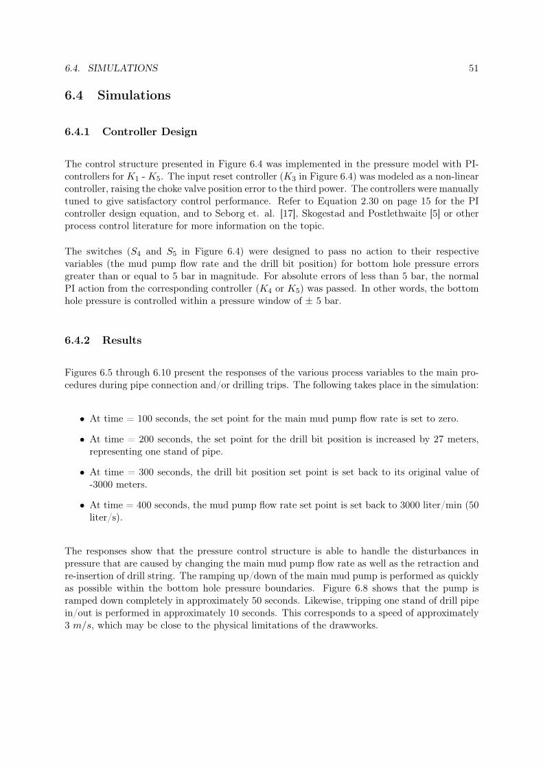
6.4. SIMULATIONS 51
6.4 Simulations
6.4.1 Controller Design
The control structure presented in Figure 6.4 was implemented in the pressure model with PI-controllers for K1 - K5. The input reset controller (K3 in Figure 6.4) was modeled as a non-linearcontroller, raising the choke valve position error to the third power. The controllers were manuallytuned to give satisfactory control performance. Refer to Equation 2.30 on page 15 for the PIcontroller design equation, and to Seborg et. al. [17], Skogestad and Postlethwaite [5] or otherprocess control literature for more information on the topic.
The switches (S4 and S5 in Figure 6.4) were designed to pass no action to their respectivevariables (the mud pump flow rate and the drill bit position) for bottom hole pressure errorsgreater than or equal to 5 bar in magnitude. For absolute errors of less than 5 bar, the normalPI action from the corresponding controller (K4 or K5) was passed. In other words, the bottomhole pressure is controlled within a pressure window of ± 5 bar.
6.4.2 Results
Figures 6.5 through 6.10 present the responses of the various process variables to the main pro-cedures during pipe connection and/or drilling trips. The following takes place in the simulation:
• At time = 100 seconds, the set point for the main mud pump flow rate is set to zero.
• At time = 200 seconds, the set point for the drill bit position is increased by 27 meters,representing one stand of pipe.
• At time = 300 seconds, the drill bit position set point is set back to its original value of-3000 meters.
• At time = 400 seconds, the mud pump flow rate set point is set back to 3000 liter/min (50liter/s).
The responses show that the pressure control structure is able to handle the disturbances inpressure that are caused by changing the main mud pump flow rate as well as the retraction andre-insertion of drill string. The ramping up/down of the main mud pump is performed as quicklyas possible within the bottom hole pressure boundaries. Figure 6.8 shows that the pump isramped down completely in approximately 50 seconds. Likewise, tripping one stand of drill pipein/out is performed in approximately 10 seconds. This corresponds to a speed of approximately3 m/s, which may be close to the physical limitations of the drawworks.
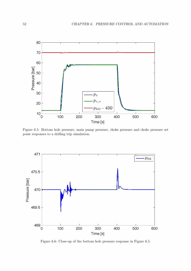
52 CHAPTER 6. PRESSURE CONTROL AND AUTOMATION
Figure 6.5: Bottom hole pressure, main pump pressure, choke pressure and choke pressure setpoint responses to a drilling trip simulation.
Figure 6.6: Close-up of the bottom hole pressure response in Figure 6.5.
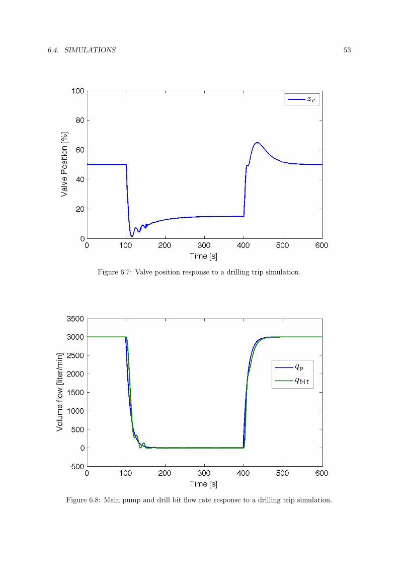
6.4. SIMULATIONS 53
Figure 6.7: Valve position response to a drilling trip simulation.
Figure 6.8: Main pump and drill bit flow rate response to a drilling trip simulation.
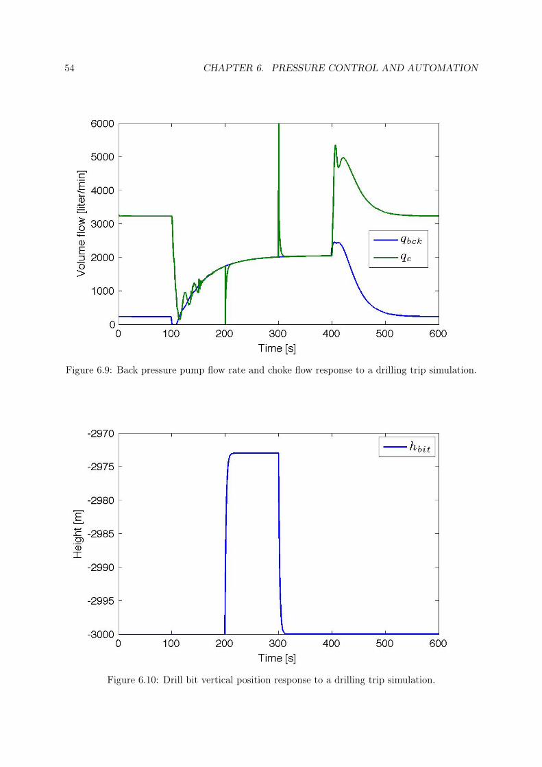
54 CHAPTER 6. PRESSURE CONTROL AND AUTOMATION
Figure 6.9: Back pressure pump flow rate and choke flow response to a drilling trip simulation.
Figure 6.10: Drill bit vertical position response to a drilling trip simulation.
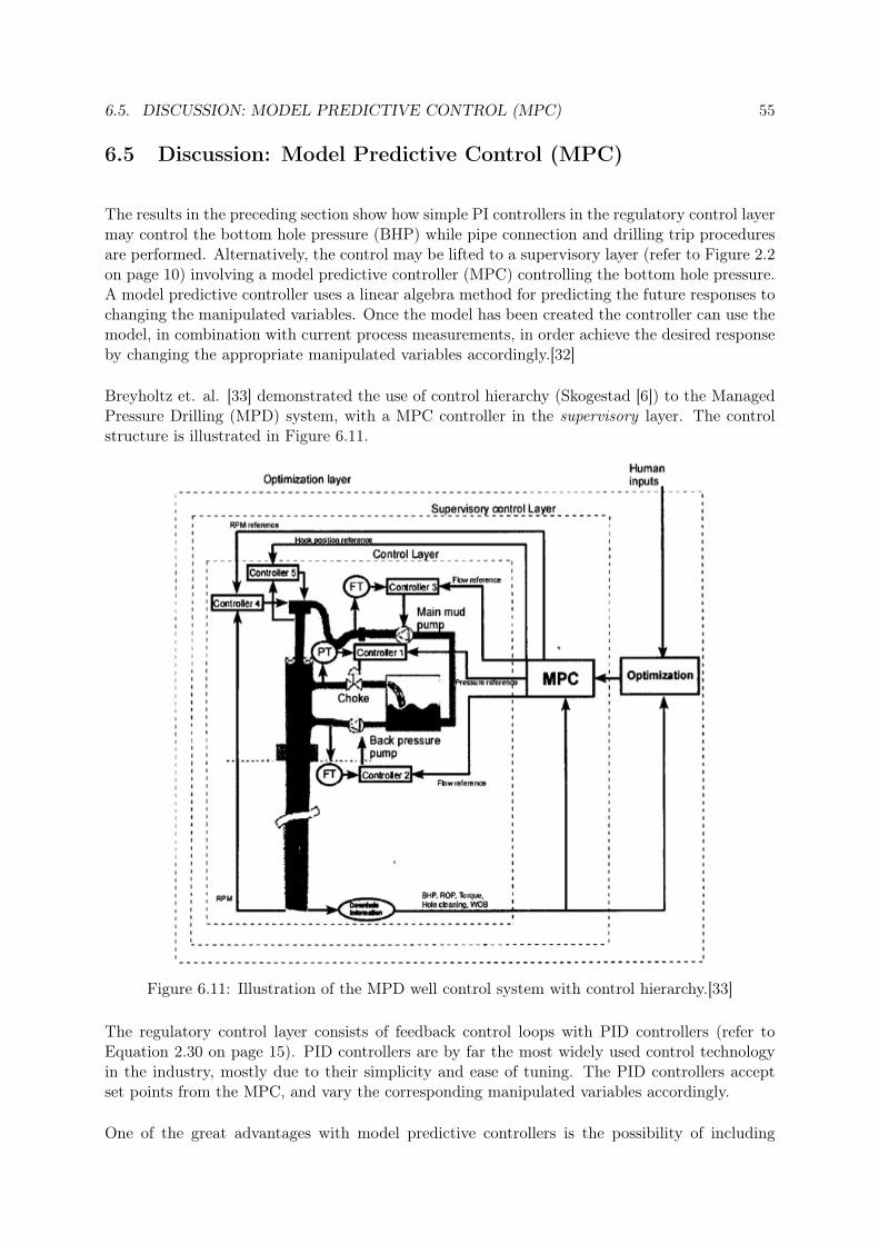
6.5. DISCUSSION: MODEL PREDICTIVE CONTROL (MPC) 55
6.5 Discussion: Model Predictive Control (MPC)
The results in the preceding section show how simple PI controllers in the regulatory control layermay control the bottom hole pressure (BHP) while pipe connection and drilling trip proceduresare performed. Alternatively, the control may be lifted to a supervisory layer (refer to Figure 2.2on page 10) involving a model predictive controller (MPC) controlling the bottom hole pressure.A model predictive controller uses a linear algebra method for predicting the future responses tochanging the manipulated variables. Once the model has been created the controller can use themodel, in combination with current process measurements, in order achieve the desired responseby changing the appropriate manipulated variables accordingly.[32]
Breyholtz et. al. [33] demonstrated the use of control hierarchy (Skogestad [6]) to the ManagedPressure Drilling (MPD) system, with a MPC controller in the supervisory layer. The controlstructure is illustrated in Figure 6.11.
Figure 6.11: Illustration of the MPD well control system with control hierarchy.[33]
The regulatory control layer consists of feedback control loops with PID controllers (refer toEquation 2.30 on page 15). PID controllers are by far the most widely used control technologyin the industry, mostly due to their simplicity and ease of tuning. The PID controllers acceptset points from the MPC, and vary the corresponding manipulated variables accordingly.
One of the great advantages with model predictive controllers is the possibility of including

56 CHAPTER 6. PRESSURE CONTROL AND AUTOMATION
constraints to the controller. Thus, if the choke valve (zc) reaches its constraints, the MPCcontroller can automatically compensate by providing a higher set point to the back pressurepump (qbck) controller. Similarly, the main mud pump flow rate may be used to control thepressure profile during drilling operation, but is shut down by the MPC prior to pipe connectionsor drilling trip procedures. The MPC controller will accept operator inputs for the hook position(bit position) and main mud pump set points when applicable, and manipulate the processvariable in order to reach the new set points while simultaneously controlling the bottom holepressure.
The MPC controller could probably handle all the control tasks by itself, but the modeling effortis greatly reduced by the PID controllers in the regulatory layer. The model dependency is infact one of the major disadvantages with model predictive controllers, as an accurate model isnecessary to obtain good results. When working properly, a MPC will outperform the alternativestrategy of a feedback control structure. However, the MPC performance is dependent on manyparameters being correctly formulated, such as the model itself, the prediction horizon, controlhorizon, manipulated input weighting and sample time. Therefore, a feedback control structureconsisting of PI controllers was presented in this thesis work as a feasible alternative.

Chapter 7
Conclusions and Further Work
7.1 Conclusions
The thesis work has involved a extensive search for- and review of drilling literature, in orderto learn the process and the challenges that are faced during drilling operations. A steady-statemodel of the drilling process was modeled based on equations found in literature. Most of thedrilling equations used are empirical and require parameter estimation for a large number ofparameters. These estimates were made based on reported values in drilling literature, as wellas trial-and-error procedures to re-produce realistic drilling results from the model.
The objective function, or cost function, of the drilling process was determined based on drillingliterature, reasoning and analysis. The cost function was to reflect all parts of the drilling process,not only the active drilling time. Analysis of the objective function led to the separation of thedrilling operations into two operating modes: Active drilling operations, and pipe connectionsand drilling trips. The reason for separating the process into two operating modes was thedifference in control objectives. Thus, the optimization the active drilling operations and thepipe connections and trips were analyzed separately.
7.1.1 Optimal Controlled Variables
The drilling process was optimized for given parameters representing the drilling conditions. Theconstraints on the bottom hole pressure and mud circulation rate were active at the optimum.It is optimal to control active constraints, so two degrees of freedom were removed from furtheranalysis. The bottom hole pressure was controlled by the choke pressure, while the main mudpump flow rate was kept constant.
The expected disturbances were applied and the unconstrained drilling process was re-optimizedin order to determine the optimal self-optimizing controlled variables. The results showed thatthere is negligible gain in combining more than four measurements in the controlled variables.The optimal CV’s using single measurements and measurement combinations of three and fourmeasurements are presented in Table 7.1. The maximum loss in hours is included in the rightmost
57

58 CHAPTER 7. CONCLUSIONS AND FURTHER WORK
column.
Table 7.1: Optimal Controlled Variables
Description CV’s (CV1 on top, CV2 on bottom) Max. loss
4 measurements 0.70 R + 0.52 T + 0.50 W - 0.01 N 2.02-0.19 R + 0.76 T - 0.36 W + 0.50 N
3 measurements 0.83 R + 0.56 T - 0.05 N 3.15-0.51 R + 0.64 T + 0.58 N
Single measurements W 6.24P
Constant Inputs W 11.44N
For single measurement controlled variables, the results show that it is optimal to control thetopdrive power by manipulating the drill string rotational speed, and keep the weight on bit(WOB) constant. Combining several measurements will give a lower loss, but the loss is small(approximately 1 % of the active drilling time) and the complexity of the control structure willincrease.
A constant input policy will only have a loss of approximately 1 % of the active drilling timecompared to the optimal single measurement control structure, thus raising the question ofwhether or not implementing a control structure is worth the added complexity to the drillingsystem. However, problems with stick-slip phenomenon are prone in drilling systems operatingwith a constant drill string rotational speed. Several authors have proposed stick-slip preventiontechniques involving a varying rotational drill string speed. Therefore, it is likely that a controlstructure a varying drill string RPM will be optimal.
7.1.2 Pressure Control & Automation
A feedback control structure involving PI controllers was designed for controlling the bottomhole pressure, using the back pressure pump and the choke valve opening as manipulated inputs.The time spent performing pipe connections and drilling trips is an important factor in theoptimization of the drilling process. It is important that these procedures are performed as fastas possible, while keeping the bottom hole pressure within its margins. Procedures that involveroom for automation are the ramping down/up of the main mud pump, as well as tripping thedrill string in and out of the well. An automatic control system was designed to perform theseprocedures as fast as possible, while keeping the bottom hole pressure within a pressure windowof ±5 bar. The control structure was able to perform the tasks at speeds that are likely tobe close to the physical limitations of the process equipment. Thus, we may conclude that theperformance is satisfactory.
An alternative solution of implementing a model predictive controller was discussed. The MPCwill perform as a supervisory controller in a hierarchical structure. An MPC will give superior re-sults compared to a stand-alone regulatory control structure, but requires an increased modelingeffort and is more error prone.
7.2. FURTHER WORK 59
7.2 Further work
The drilling process involves many challenges and complications that make it difficult to assessthe process completely and take everything into account. The thesis work has been carried outwithout any prior experience with drilling processes, thus consisting of rather simplified models.Further studies of the drilling process and industry experience would undoubtedly result in amore detailed drilling model, improving the accuracy of the results.
It would be interesting to test the model and results of this thesis in real-life drilling operations. Abrute-force analysis should be performed, implementing control of the self-optimizing controlledvariables determined in this thesis. The results would show whether or not the theoretical resultshold for a real-life drilling scenario. Similarly, the real-life performance of the suggested feedbackpressure control structure should be tested.
The results will also show whether the simple steady-state model is adequate in describing thedrilling process. In case improvements are required, the results may give insight to which areasof the model are weaker, and which are stronger.

60 CHAPTER 7. CONCLUSIONS AND FURTHER WORK
Bibliography
[1] World Energy Outlook. International Energy Agency, 2009.
[2] Øyvind N. Stamnes. Adaptive observer for bottomhole pressure during drilling. M. Sc.thesis, NTNU, Department of Engineering Cybernetics, 2007.
[3] Mark S. Gockenbach. Lecture: Introduction to sequential quadratic programming. Michi-gan Technological University, http://www.math.mtu.edu/~msgocken/ma5630spring2003/lectures/sqp1/sqp1.pdf.
[4] Moritz Kuhn. The Karush-Kuhn-Tucker Theorem. CDSEM Uni Mannheim, 2006.
[5] Sigurd Skogestad and Ian Postlethwaite. Multivariable Feedback Control: Analysis andDesign. John Wiley & Sons, Ltd, second edition, 2005.
[6] Sigurd Skogestad. Control structure design for complete chemical plants. Computers andChemical Engineering, 28:219–234, 2004.
[7] Sigurd Skogestad. Plantwide control: the search for the self-optimizing control structure.Journal of Process Control, 10:487–507, 2000.
[8] Vidar Alstad, Sigurd Skogestad, and Eduardo S. Hori. Optimal measurement combinationsas controlled variables. Journal of Process Control, 19:138–148, 2009.
[9] Ivar J. Halvorsen, Sigurd Skogestad, John C. Morud, and Vidar Alstad. Optimal Selection ofControlled Variables. Industrial Engineering Chemistry Research, 42(14):3273–3284, 2003.
[10] Vidar Alstad and Sigurd Skogestad. Null Space Method for Selecting Optimal MeasurementCombinations as Controlled Variables. Industrial Engineering Chemistry Research, 46:846–853, 2007.
[11] Ramprasad Yelchuru, Sigurd Skogestad, and Henrik Manum. MIQP formulation for Con-trolled Variable Selection in Self Optimizing Control. Submitted to DYCOPS 2010 Sympo-sium, 2010.
[12] A. T. Bourgoyne and F. S. Young. A multiple regression approach to optimal drilling andabnormal pressure detection. Society of Petroleum Engineers (SPE) Journal, pages 371–384,Aug. 1974.
[13] A.T. Bourgoyne, M.E. Chenevert, K.K. Millheim, and F.S. Young. Applied Drilling Engi-neering. Society of Petroleum Engineering (SPE), 1986.
[14] P. L. Moore. Drilling Practices Manual. Petroleum Publishing Company, Tulsa, OK, U.S.A.,1974.
61

62 BIBLIOGRAPHY
[15] S. F. Chien. Annular Velocity for Rotary Drilling Operations. In Proceedings of SPEFifth Conference on Drilling and Rock Mechanics, Jan. 5-6, 1971, pages 5–16. Society ofPetroleum Engineers (SPE), Austin, TX, U.S.A., 1971.
[16] MATLAB R2009a Documentation. The MathWorks, Inc., 2009.
[17] D. E. Seborg, T. F. Edgar, and D. A. Mellichamp. Process Dynamics and Control. JohnWiley & Sons, Ltd, second edition, 2004.
[18] Ronald L. Reed. A Monte Carlo Approach to Optimal Drilling. Society or PetroleumEngineers (SPE) Journal, 12(5):423–438, 1972.
[19] E. M. Galle and H. B. Woods. Best Constant Weight and Rotary Speed for Rotary RockBits. Drilling and Production Practice, pages 48–73, 1963.
[20] John-Morten Godhavn. Control requirements for high-end automatic MPD operations.SPE/IADC Drilling Conference and Exhibition, 17-17 March 2009, Amsterdam, The Nether-lands, 2009.
[21] Tuna Eren and M. Evren Ozbayoglu. Real Time Optimization of Drilling Parameters DuringDrilling Operations. SPE Oil and Gas India Conference and Exhibition, 20-22 January 2010,Mumbai, India, 2010.
[22] Eva María Navarro-López and Rodolfo Suárez. Practical approach to modelling and con-trolling stick-slip oscillations in oilwell drillstrings. In Proceedings of the 2004 IEEE In-ternational Conference on Control Applications, 2-4 September. Institute of Electrical andElectronics Engineers (IEEE), Taipei, Taiwan, 2004.
[23] Ahmet S. Yigit and Andreas P. Christoforou. Stick-Slip and Bit-Bounce Interaction in Oil-Well Drillstrings. Journal of Energy Resources Technology, 128:268–274, December 2006.
[24] F. Abdulgalil and H. Siguerdidjane. Nonlinear Friction Compensation Design for Suppress-ing Stick Slip Oscillations in Oil Well Drillstrings. In Proceedings of DYCOPS 7, 5-7 July,2004. International Federation of Automatic Control (IFAC), Cambridge, MA, U.S.A., 2004.
[25] R. W. Tucker and C. Wang. On the Effective Control of Torsional Vibrations in DrillingSystems. Journal of Sound and Vibration, 244(1):101–122, 1999.
[26] G. W. Halsey, A. Kyllingstad, and A. Kylling. Torque Feedback Used to Cure Slip-StickMotion. In Proceedings of the 63rd SPE Annual Technical Conference and Exhibition, 2-5October, 1988. Society of Petroleum Engineers (SPE), Houston, TX, U.S.A., 1988.
[27] Kazem Javanmardi and D. T. Gaspard. Application of Soft-Torque Rotary Table in MobileBay. SPE/IADC Drilling Conference, 18-21 February, New Orleans, LA, U.S.A., 1992.
[28] R. I. Leine. Literature Survey on Torsional Drillstring Vibrations. Internal Report - Divisionof Computational and Experimental Mechanics, Department of Mechanical Engineering,Eindhoven University of Technology, Eindhoven, The Netherlands, 1997.
[29] Glenn-Ole Kaasa. A Simple Dynamic Model of Drilling for Control. Technical Report,Statoil Research Centre, Porsgrunn, Norway, 2007.
[30] G. Nygaard, M. Nikolaou, E. H. Vefring, H. Siahaan, and Ø . Breyholtz. Control Hierarchyfor Automated Co-ordinated Control of Drilling Equipment. Report - International ResearchInstitute of Stavanger (IRIS), 2010.

BIBLIOGRAPHY 63
[31] Øyvind Nistad Stamnes, Jing Zhou, Glenn-Ole Kaasa, and Ole Morten Aamo. Adaptiveobserver design for the bottomhole pressure of a managed pressure drilling system. InProceedings of 47th IEEE Conference on Decision and Control, 9-11 December, pages 2961–2966. Institute of Electrical and Electronics Engineers (IEEE), Cancun, Mexico, 2008.
[32] B. Wayne Bequette. Process Control: Modeling, Design and Simulation. Prentice Hall, 2003.
[33] Øyvind Breyholtz, Gerhard Nygaard, Hardy Siahaan, and Michael Nikolaou. ManagedPressure Drilling: A Multi-Level Control Approach. SPE Intelligent Energy Conference andExhibition, 23-25 March 2010, Utrecht, The Netherlands, 2010.

64 BIBLIOGRAPHY

Appendix A
Nomenclature
Table A.1: Nomenclature
Symbol Description Unitβ Bulk modulus barµ Viscosity Pa·sρf Effective mud density kg/m3
ρ / ρm Mud density kg/m3
ρs Formation density kg/m3
θ1 Annulus friction parameter kg/m4 sθ2 Drill string friction parameter kg/m7
Aa Cross-sectional area of annulus m2
D Well depth mdb Drill bit diameter mdH Hydraulic diameter mdi Drill string inner diameter mdp Drilled particle diameter mds Drill string outer diameter mFbo Buoyant force NFc Cutting force NFg Gravitational force NFj Hydraulic jet impact force Nf Friction factor -g Acceleration due to Earth gravity m/s2
J(u, d) Objective function value hoursK Bit life-time constant hoursKc Valve flow constant m2
k0c Specific cutting force constant N/tonm2
kc Specific cutting force N/m2
M Mass coefficient 105 kg/m4
NRe Reynolds number -N Drill string rotational speed min−1
P Power kWpbh Bottom hole pressure bar
Continued on next page
65
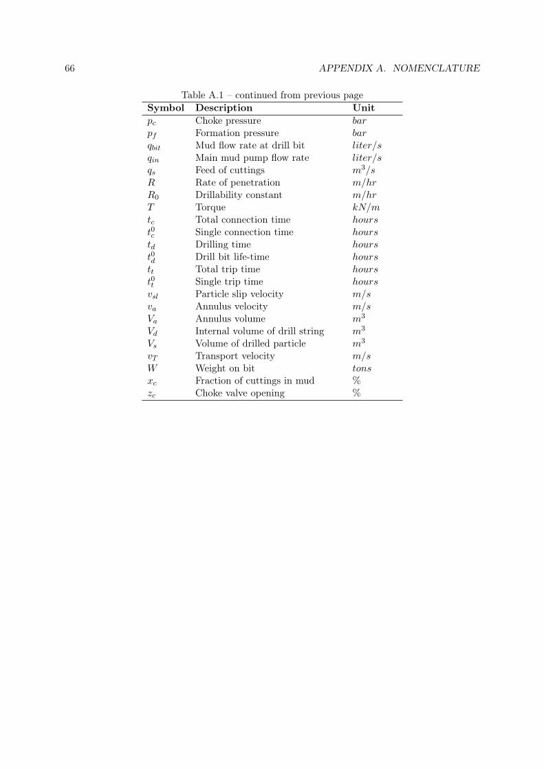
66 APPENDIX A. NOMENCLATURE
Table A.1 – continued from previous pageSymbol Description Unitpc Choke pressure barpf Formation pressure barqbit Mud flow rate at drill bit liter/sqin Main mud pump flow rate liter/sqs Feed of cuttings m3/sR Rate of penetration m/hrR0 Drillability constant m/hrT Torque kN/mtc Total connection time hourst0c Single connection time hourstd Drilling time hourst0d Drill bit life-time hourstt Total trip time hourst0t Single trip time hoursvsl Particle slip velocity m/sva Annulus velocity m/sVa Annulus volume m3
Vd Internal volume of drill string m3
Vs Volume of drilled particle m3
vT Transport velocity m/sW Weight on bit tonsxc Fraction of cuttings in mud %zc Choke valve opening %

Appendix B
Miscellaneous Calculation Matrices
The gain matrix, sensitivity matrix and various other matrices used in the calculations arepresented below.
∇2J(u) = Juu =[1.88160.11590.11590.0222
]
G =
0.5046 0.10560.9975 010.4167 3.45360.0331 0.00691.0000 0
0 1.0000
S1 =
0.1005 0 0 0 0 00 0.0505 0 0 0 00 0 0.0102 0 0 00 0 0 0.8727 0 00 0 0 0 0.2888 00 0 0 0 0 0.0241
G′ = S1G =
0.05 0.010.05 00.11 0.040.03 0.010.29 0
0 0.02
67
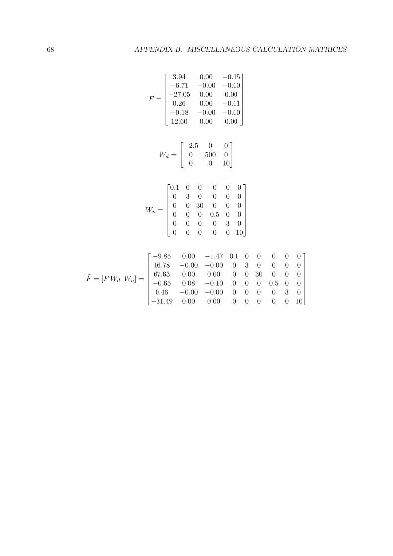
68 APPENDIX B. MISCELLANEOUS CALCULATION MATRICES
F =
3.94 0.00 −0.15−6.71 −0.00 −0.00−27.05 0.00 0.00
0.26 0.00 −0.01−0.18 −0.00 −0.0012.60 0.00 0.00
Wd =
−2.5 0 00 500 00 0 10
Wn =
0.1 0 0 0 0 00 3 0 0 0 00 0 30 0 0 00 0 0 0.5 0 00 0 0 0 3 00 0 0 0 0 10
F = [F Wd Wn] =
−9.85 0.00 −1.47 0.1 0 0 0 0 016.78 −0.00 −0.00 0 3 0 0 0 067.63 0.00 0.00 0 0 30 0 0 0−0.65 0.08 −0.10 0 0 0 0.5 0 00.46 −0.00 −0.00 0 0 0 0 3 0−31.49 0.00 0.00 0 0 0 0 0 10
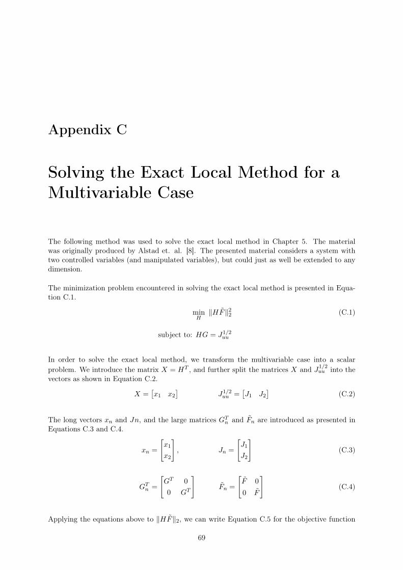
Appendix C
Solving the Exact Local Method for aMultivariable Case
The following method was used to solve the exact local method in Chapter 5. The materialwas originally produced by Alstad et. al. [8]. The presented material considers a system withtwo controlled variables (and manipulated variables), but could just as well be extended to anydimension.
The minimization problem encountered in solving the exact local method is presented in Equa-tion C.1.
minH‖HF‖22 (C.1)
subject to: HG = J1/2uu
In order to solve the exact local method, we transform the multivariable case into a scalarproblem. We introduce the matrix X = HT , and further split the matrices X and J1/2
uu into thevectors as shown in Equation C.2.
X =[x1 x2
]J1/2
uu =[J1 J2
](C.2)
The long vectors xn and Jn, and the large matrices GTn and Fn are introduced as presented in
Equations C.3 and C.4.
xn =
[x1
x2
], Jn =
[J1
J2
](C.3)
GTn =
[GT 00 GT
]Fn =
[F 0
0 F
](C.4)
Applying the equations above to ‖HF‖2, we can write Equation C.5 for the objective function
69

70APPENDIX C. SOLVING THE EXACT LOCAL METHOD FOR A MULTIVARIABLE CASE
of the minimization problem.
‖HF‖22 =
∣∣∣∣∣∣∣∣∣∣[xT
1 F
xT2 F
]∣∣∣∣∣∣∣∣∣∣2
2
= ‖[xT
1 F xT2 F]‖22 (C.5)
= ‖xTn Fn‖22 = ‖F T
n xn‖22 = xTn FnF
Tn xn (C.6)
Since Juu is a symmetric positive definite matrix at an unconstrained optimum, J1/2uu is also a
symmetric positive definite matrix. Thus, we can write HG = GTHT = GTX = J1/2uu .
Further:GTX =
[GTx1 GTx2
]=[J1 J2
]Thus, the constraints may be written as shown in Equation C.7.
[GTx1
GTx2
]=[J1J2
]⇒ Gnxn = Jn (C.7)
The result is that the optimization problem in Equation C.1 may be re-written as Equation C.8and the quadratic program can easily be solved, e.g. using the MATLAB® function quadprog.
minxn
xTn FnF
Tn xn (C.8)
subject to: Gnxn = Jn
The xn matrix is finally reshaped back to form the optimal measurement combination matrixH, where the first row of H is found as the top half of the column vector xn while the secondrow of H is the bottom part.
H =
[xT
1
xT2
]

Appendix D
Results of the Exact Local Method
The results of the exact local method for 2-6 measurement combinations are presented inTables D.1 through D.5.
Table D.1: Optimal Combinations of 6 Measurements
H matrix Max. loss0.75 0.40 0.02 0.00 0.53 -0.07 1.87-0.39 -0.11 0.16 -0.00 -0.77 0.46
Table D.2: Optimal Combinations of 5 Measurements
H matrix Max. loss0.00 0.02 0.01 0.83 0.55 0.01 4.830.00 0.04 0.10 -0.64 -0.72 0.240.58 0.00 0.04 0.00 0.80 -0.14 2.71-0.32 0.00 0.15 -0.00 -0.81 0.460.70 0.52 0.00 0.00 0.50 -0.01 2.02-0.19 0.76 0.00 -0.00 -0.36 0.500.75 0.40 0.02 0.00 0.53 -0.07 1.87-0.39 -0.11 0.16 0.00 -0.77 0.460.88 0.47 0.01 0.00 0.00 -0.10 3.04-0.81 -0.37 0.13 -0.00 0.00 0.440.62 0.49 -0.00 0.00 0.61 0.00 2.270.12 -0.49 0.15 0.00 -0.85 0.00
71

72 APPENDIX D. RESULTS OF THE EXACT LOCAL METHOD
Table D.3: Optimal Combinations of 4 Measurements
H matrix Max. loss0.00 0.00 0.01 0.82 0.57 0.01 4.850.00 0.00 0.10 -0.68 -0.69 0.230.00 0.09 0.00 0.83 0.55 0.03 4.970.00 0.69 0.00 -0.41 -0.46 0.390.00 0.01 0.01 0.00 1.00 0.03 5.130.00 0.06 0.12 0.00 -0.94 0.300.00 0.03 0.00 1.00 0.00 -0.00 56.280.00 -0.03 0.01 -1.00 0.00 0.030.00 -0.01 0.01 0.85 0.53 0.00 4.860.00 -0.58 0.15 0.39 -0.70 0.00-0.06 0.00 0.00 -0.00 1.00 0.06 8.50-0.70 0.00 0.00 -0.00 0.62 0.350.58 0.00 0.04 0.00 0.80 -0.14 2.71-0.32 0.00 0.15 0.00 -0.81 0.460.96 0.00 0.06 0.00 0.00 -0.27 6.04-0.82 0.00 0.10 -0.00 0.00 0.560.12 0.00 0.02 0.00 0.99 0.00 4.410.38 0.00 0.08 0.00 -0.92 0.000.70 0.52 0.00 0.00 0.50 -0.01 2.02-0.19 0.76 0.00 0.00 -0.36 0.500.83 0.56 0.00 0.00 0.00 -0.05 3.15-0.51 0.64 0.00 -0.00 0.00 0.580.62 0.48 0.00 0.00 0.62 0.00 9.660.54 0.41 0.00 0.00 -0.74 0.000.88 0.47 0.01 0.00 0.00 -0.10 3.04-0.81 -0.37 0.13 0.00 0.00 0.440.62 0.49 -0.00 0.00 0.61 0.00 2.270.12 -0.49 0.15 0.00 -0.85 0.000.75 0.66 -0.01 0.00 0.00 0.00 4.61-0.42 -0.90 0.14 -0.00 0.00 0.00

73
Table D.4: Optimal Combinations of 3 Measurements
H matrix Max. loss0.00 0.00 0.00 -0.46 0.89 0.05 10.310.00 0.00 0.00 -1.00 0.05 0.040.00 0.00 0.01 0.00 1.00 0.02 5.130.00 0.00 0.13 0.00 -0.95 0.290.00 0.00 0.00 1.00 0.00 -0.02 60.890.00 0.00 0.00 -1.00 0.00 0.040.00 0.00 0.01 0.90 0.44 0.00 4.870.00 0.00 0.01 0.99 -0.14 0.000.00 0.12 0.00 0.00 0.99 0.06 5.270.00 0.75 0.00 0.00 -0.51 0.410.00 0.05 0.00 1.00 0.00 -0.00 56.740.00 0.05 0.00 -1.00 0.00 0.060.00 0.03 0.00 1.00 0.03 0.00 107.640.00 0.03 0.00 1.00 -0.05 0.000.00 1.00 0.05 0.00 0.00 -0.08 160.090.00 -0.85 0.13 0.00 0.00 0.510.00 -0.07 0.02 0.00 1.00 0.00 5.200.00 -0.64 0.16 0.00 -0.75 0.000.00 0.05 -0.00 1.00 0.00 0.00 57.370.00 -0.11 0.02 -0.99 0.00 0.00-0.06 0.00 0.00 0.00 1.00 0.06 8.50-0.70 0.00 0.00 0.00 0.62 0.350.99 0.00 0.00 0.00 0.00 -0.10 165.270.68 0.00 0.00 0.00 0.00 0.730.49 0.00 0.00 0.00 0.87 0.00 84.740.86 0.00 0.00 0.00 -0.52 0.000.96 0.00 0.06 0.00 0.00 -0.27 6.04-0.82 0.00 0.10 0.00 0.00 0.560.12 0.00 0.02 0.00 0.99 0.00 4.410.38 0.00 0.08 0.00 -0.92 0.001.00 0.00 -0.04 0.00 0.00 0.00 2077.66-1.00 0.00 0.07 -0.00 0.00 0.000.83 0.56 0.00 0.00 0.00 -0.05 3.15-0.51 0.64 0.00 0.00 0.00 0.580.62 0.48 0.00 0.00 0.62 0.00 9.660.54 0.41 0.00 0.00 -0.74 0.000.49 0.87 0.00 0.00 0.00 0.00 227.970.86 -0.52 0.00 0.00 0.00 0.000.75 0.66 -0.01 0.00 0.00 0.00 4.61-0.42 -0.90 0.14 0.00 0.00 0.00

74 APPENDIX D. RESULTS OF THE EXACT LOCAL METHOD
Table D.5: Optimal Combinations of 2 Measurements
H matrix Max. loss0.00 0.00 0.00 0.00 1.00 0.06 11.440.00 0.00 0.00 0.00 0.49 0.870.00 0.00 0.00 1.00 0.00 -0.00 475.950.00 0.00 0.00 1.00 0.00 0.040.00 0.00 0.00 1.00 0.06 0.00 184.940.00 0.00 0.00 1.00 -0.02 0.000.00 0.00 0.33 0.00 0.00 -0.94 168.840.00 0.00 0.07 0.00 0.00 1.000.00 0.00 0.02 0.00 1.00 0.00 6.240.00 0.00 0.12 0.00 -0.99 0.000.00 0.00 -0.00 1.00 0.00 0.00 3790.860.00 0.00 0.00 -1.00 0.00 0.000.00 1.00 0.00 0.00 0.00 0.06 161.900.00 0.49 0.00 0.00 0.00 0.87NaN NaN NaN NaN NaN NaN NaNNaN NaN NaN NaN NaN NaN0.00 0.06 0.00 1.00 0.00 0.00 278.100.00 -0.02 0.00 1.00 0.00 0.000.00 1.00 0.02 0.00 0.00 0.00 160.700.00 -0.99 0.12 0.00 0.00 0.000.99 0.00 0.00 0.00 0.00 -0.10 165.270.68 0.00 0.00 0.00 0.00 0.730.49 0.00 0.00 0.00 0.87 0.00 84.740.86 0.00 0.00 0.00 -0.52 0.000.03 0.00 0.00 -1.00 0.00 0.00 NaN-0.03 0.00 0.00 1.00 0.00 0.001.00 0.00 -0.04 0.00 0.00 0.00 2077.66-1.00 0.00 0.07 0.00 0.00 0.000.49 0.87 0.00 0.00 0.00 0.00 227.970.86 -0.52 0.00 0.00 0.00 0.00

Appendix E
MATLAB files
The MATLAB scripts and functions that were used in order to produce the results of this thesiswork are attached on the CD-ROM marked Appendix E. A list of the file names and descriptionsare presented in Table E.1.
Table E.1: List of MATLAB Files
File name Descriptionmain4u.m Main script for optimizing the drilling process with 4 inputsdrilling4u.m Steady-state drilling model accepting 4 inputsdrillsolve4u.m Function used to solve equation system in drilling4u.mobjfun4u.m Objective function accepting 4 inputsconstraints.m Drilling model constraintsmain.m Main script for optimizing the unconstrained drilling process with 2 inputsdrilling.m Steady-state drilling model accepting 2 inputsdrillsolve.m Function used to solve equation system in drilling.mobjfun.m Objective function accepting 2 inputsmsv.m Function used to solve the method of maximizing the minimum singular valueexactlocal.m Function used to solve the exact local methodrunSim.m Main script for running control simulations on dynamic pressure modelcalcf.m Function used to calculate the dynamics of the pressure model
75

76 APPENDIX E. MATLAB FILES
main4u.m:
1 %Script for optimizing the drilling process with 4 inputs2 %Needs external functions drilling4u.m, drillsolve4u.m3 %objfun4u.m and constraints.m.4 %DEH − 20105
6 clear all7 close all8 clc9
10 global db Wdbmax tt0 dstring Wdbt R0 K kc D dp Aa g rho rhos theta111
12 %Parameters:13 db = 0.254; %Bit diameter, m14 Wdbmax = 178.583; %Maximum WOB per m diameter, tons/m15 tt0 = 10; %Trip time, hours16 dstring = 0.1; %Diameter of drill string, m17 D = 3000; %Depth, m18 Aa = (db^2−dstring^2)*pi/4; %Cross−sectional area of annulus, m219 g = 9.81; %Gravity20 R0 = 5; %Formation drillability, m/hr21 tempR0 = R0;22 K = 15*R0; %Formation abrasiveness constant, hours23 kc = 5e5/R0; %Specific cutting force, N/m2−ton24 Wdbt = 63/R0; %Threshold WOB per m diameter, tons/m25 theta1 = 900; %Friction parameter26 rhos = 2700; %Formation density, kg/m327 rho = 1400; %Mud density, kg/m328 dp = 0.005; %Particle diameter, m29
30 %Optimization:31 u0 = [30; %WOB, tons32 100; %RPM33 40; %qmud, l/s34 10]; %pc, bar35
36 lb = [0; 0; 0; 0];37 ub = [Wdbmax*db; 200; 50; 100];38 options = optimset('Display','iter','TolFun',1e−12,'MaxFunEvals',300);39 [u,fval,exitflag,output,lambda,grad,hessian] = fmincon(@objfun4u, u0,...40 [],[],[],[],lb,ub,@constraints,options)41 Juu = hessian;42
43 %Nominal optimum u and y:44 y0 = drilling4u(u)

77
drilling4u.m:
1 function y = drilling4u(u)2 %Function that calculates drilling model equations.3 %Run main4u.m4 %DEH − 20105
6 global db dstring kc WOB RPM qmud pc7
8 y = zeros(9,1);9
10 WOB = u(1);11 RPM = u(2);12 qmud = u(3);13 pc = u(4);14
15 x0 = [15;1;460];16 res = fsolve(@drillsolve4u,x0);17 y(1) = res(1); %ROP18 y(4) = res(2); %Cuttings fraction19 y(5) = res(3); %Mud flow20 F = u(1)/db*kc*db^2*pi/4; %Force, N, function of WOB and formation strength21 y(2) = F*dstring/2000; %Torque, kNm.22 y(3) = y(2)*2*pi*u(2)/60; %Power, kW23 y(6) = u(1);24 y(7) = u(2);25 y(8) = u(3);26 y(9) = u(4);
drillsolve4u.m:
1 function f = drillsolve4u(y)2 %Function that solves system of drilling equations.3 %Run main4u.m4 %DEH − 20105
6 global db Aa dp g Wdbt R0 rho rhos theta1 D WOB RPM qmud pc7
8 f = zeros(3,1);9
10 newrho = rho*(1−y(2)/100) + rhos*y(2)/100; %rhof, kg/m311 bhp = pc + theta1*qmud/1000 + newrho*g*D/1e5; %BHP, bar12
13 An = 3*pi*0.01^2/4; %nozzle x−sec area, m214 Fj = qmud^2*rho/An/1e6; %hydraulic jet impact force, N15 ROP = R0*(WOB/db−Wdbt)/(71.433−Wdbt)*(RPM/60)^0.7*exp(0.01*...16 (470−bhp))*(Fj/4448.22)^.3;17
18 va = qmud/1000/Aa; %annulus velocity, m/s19 vslip = sqrt(8/9*g*dp*(rhos−newrho)/rho); %slip velocity, m/s20 vT = va − vslip; %transport velocity, m/s21 qs = ROP*pi/4*db^2*1000/3600; %cuttings feed rate, l/s22 xc = qs/1000/Aa/vT*100; %cuttings fraction23
24 f(1) = ROP − y(1);25 f(2) = xc − y(2);26 f(3) = bhp − y(3);

78 APPENDIX E. MATLAB FILES
objfun4u.m:
1 function f = objfun4u(u)2 %Objective function for optimization of the drilling process.3 %Run main4u.m4 %DEH5
6 global db Wdbmax tt0 K D7
8 y = drilling4u(u);9 R = y(1);
10
11 td0 = K*(60/u(2))^1.7*(Wdbmax−u(1)/db)/(Wdbmax−71.433); %bit life−time12 f = D*(1/R + tt0/(R*td0)); %J, objective function
constraints.m:
1 function [C Ceq] = constraints(x)2 %Function containing the drilling process constraints.3 %Run main4u.m4 %DEH − 20105
6 y = drilling4u(x);7
8 Ceq = []; %no equality constraints9 C = zeros(2,1);
10
11 C(1) = 470 − y(5);12 C(2) = y(5) − 480;
main.m:
1 %Script for optimizing drilling process with 2 inputs2 %Needs external functions drilling.m, drillsolve.m, objfun.m3 %msv.m and exactlocal.m.4 %DEH − 20105
6 clear all7 close all8 clc9
10 global db Wdbmax tt0 dstring Wdbt R0 K kc D bhp qmud dp Aa g rho rhos11
12 %Parameters:13 db = 0.254; %Bit diameter, m14 Wdbmax = 178.583; %Maximum WOB per m diameter, tons/m15 tt0 = 10; %Trip time, hours16 dstring = 0.1; %Diameter of drill string, m17 D = 3000; %Depth18 Aa = (db^2−dstring^2)*pi/4; %Cross−sectional area of annulus, m219 g = 9.81; %Gravity20 R0 = 5; %Formation drillability, m/hr21 tempR0 = R0;22 K = 15*R0; %Formation abrasiveness constant, hours23 kc = 5e5/R0; %Specific cutting force, N/m2−ton24 Wdbt = 63/R0; %Threshold WOB per m diameter, tons/m
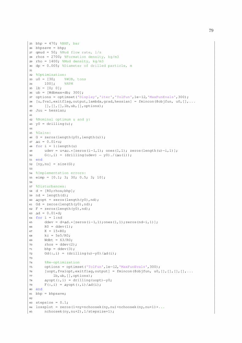
79
25 bhp = 470; %BHP, bar26 bhpsave = bhp;27 qmud = 50; %Mud flow rate, l/s28 rhos = 2700; %Formation density, kg/m329 rho = 1400; %Mud density, kg/m330 dp = 0.005; %Diameter of drilled particle, m31
32 %Optimization:33 u0 = [30; %WOB, tons34 100]; %RPM35 lb = [0; 0];36 ub = [Wdbmax*db; 300];37 options = optimset('Display','iter','TolFun',1e−12,'MaxFunEvals',300);38 [u,fval,exitflag,output,lambda,grad,hessian] = fmincon(@objfun, u0,[],...39 [],[],[],lb,ub,[],options);40 Juu = hessian;41
42 %Nominal optimum u and y:43 y0 = drilling(u);44
45 %Gains:46 G = zeros(length(y0),length(u));47 ∆u = 0.01*u;48 for i = 1:length(u)49 udev = u+∆u.*[zeros(i−1,1); ones(1,1); zeros(length(u)−i,1)];50 G(:,i) = (drilling(udev) − y0)./(∆u(i));51 end52 [ny,nu] = size(G);53
54 %Implementation errors:55 eimp = [0.1; 3; 30; 0.5; 3; 10];56
57 %Disturbances:58 d = [R0;rhos;bhp];59 nd = length(d);60 ∆yopt = zeros(length(y0),nd);61 Gd = zeros(length(y0),nd);62 F = zeros(length(y0),nd);63 ∆d = 0.01*d;64 for i = 1:nd65 ddev = d+∆d.*[zeros(i−1,1);ones(1,1);zeros(nd−i,1)];66 R0 = ddev(1);67 K = 15*R0;68 kc = 5e5/R0;69 Wdbt = 63/R0;70 rhos = ddev(2);71 bhp = ddev(3);72 Gd(:,i) = (drilling(u)−y0)/∆d(i);73
74 %Re−optimization75 options = optimset('TolFun',1e−12,'MaxFunEvals',300);76 [uopt,fvalopt,exitflag,output] = fmincon(@objfun, u0,[],[],[],[],...77 lb,ub,[],options);78 ∆yopt(:,i) = drilling(uopt)−y0;79 F(:,i) = ∆yopt(:,i)/∆d(i);80 end81 bhp = bhpsave;82
83 stepsize = 0.1;84 lossplot = zeros(1+ny+nchoosek(ny,nu)+nchoosek(ny,nu+1)+...85 nchoosek(ny,nu+2),1/stepsize+1);
80 APPENDIX E. MATLAB FILES
86
87 for a = −1:stepsize:188 c = (1+stepsize+a)/stepsize;89 ddash = a*ones(nd);90 ndash = a*ones(ny);91 Wd = diag([−2.5; 500; 10]).*ddash;92 Wn = diag(eimp).*ndash;93 Ftilde = [F*Wd Wn];94
95 %Exact Local Method:96 tempG = G;97 tempGd = Gd;98 tempFtilde = Ftilde;99 H1 = zeros(size(lossplot,1),ny);
100 H2 = zeros(size(lossplot,1),ny);101 lossvector = zeros(size(lossplot,1),2);102 [H maxloss] = exactlocal(Ftilde,Juu,G,Gd);103 H1(1,:) = H(1,:);104 H2(1,:) = H(2,:);105 lossvector(1,:) = maxloss;106
107 for i=1:ny108 G(i,:) = 0;109 Gd(i,:) = 0;110 Ftilde(i,:) = 0;111 [H maxloss] = exactlocal(Ftilde,Juu,G,Gd);112 H1(i+1,:) = H(1,:);113 H2(i+1,:) = H(2,:);114 lossvector(i+1,:) = maxloss;115 G = tempG;116 Gd = tempGd;117 Ftilde = tempFtilde;118 end119 n = ny+2;120 for j = nchoosek(1:ny,nu)'121 G(j,:) = 0;122 Gd(j,:) = 0;123 Ftilde(j,:) = 0;124 [H maxloss] = exactlocal(Ftilde,Juu,G,Gd);125 H1(n,:) = H(1,:);126 H2(n,:) = H(2,:);127 lossvector(n,:) = maxloss;128 n = n+1;129 G = tempG;130 Gd = tempGd;131 Ftilde = tempFtilde;132 end133 m = n;134 for j = nchoosek(1:ny,nu+1)'135 G(j,:) = 0;136 Gd(j,:) = 0;137 Ftilde(j,:) = 0;138 [H maxloss] = exactlocal(Ftilde,Juu,G,Gd);139 H1(m,:) = H(1,:);140 H2(m,:) = H(2,:);141 lossvector(m,:) = maxloss;142 m = m+1;143 G = tempG;144 Gd = tempGd;145 Ftilde = tempFtilde;146 end

81
147 o = m;148 for j = nchoosek(1:ny,nu+2)'149 G(j,:) = 0;150 Gd(j,:) = 0;151 Ftilde(j,:) = 0;152 [H maxloss] = exactlocal(Ftilde,Juu,G,Gd);153 H1(o,:) = H(1,:);154 H2(o,:) = H(2,:);155 lossvector(o,:) = maxloss;156 o = o+1;157 G = tempG;158 Gd = tempGd;159 Ftilde = tempFtilde;160 end161
162 res = [H1 H2 lossvector];163
164 [C5 I5] = min(res(2:7,13));165 I5 = I5+1;166 [C4 I4] = min(res(8:22,13));167 I4 = I4+7;168 [C3 I3] = min(res(23:42,13));169 I3 = I3+22;170 [C2 I2] = min(res(43:57,13));171 I2 = I2+42;172
173 lossplot(:,round(c)) = res(:,13);174 end175
176 %Minimum Singular Value method:177 eopt = max(abs(F*Wd),[],2);178 span = eopt+eimp;179 S1 = diag(1./span);180 SG = S1*G;181 msvrank = msv(SG,Juu);182
183 %Nullspace method:184 nullspaceF = [F(3,1);F(5:6,1)];185 Hnullspace = null(nullspaceF')';186
187 lossplot2 = lossplot(:,11:21);188
189 Hmatrix = zeros(2*size(H1,1),ny);190 for i = 1:size(H1,1)191 Hmatrix(2*i−1,:) = H1(i,:);192 Hmatrix(2*i,:) = H2(i,:);193 end194
195 %Results of the exact local method196 disp(res)197
198 %Plots199 x = −1:stepsize:1;200 x2 = 0:stepsize:1;201
202 set(0,'defaultaxesfontsize',14);203 set(0,'defaulttextfontsize',14);204 set(0,'DefaultLineLineWidth',1.5);205 set(0,'DefaultFigureColor','none');206 legFontSize = 14;207 scrsz = get(0,'ScreenSize');

82 APPENDIX E. MATLAB FILES
208
209 figure('Position',[1 scrsz(4)/2 scrsz(3)/2 scrsz(4)/2])210 plot(2:6,[lossvector(I2,1),lossvector(I3,1),lossvector(I4,1),...211 lossvector(I5,1),lossvector(1,1)],'k')212 ylabel('Loss = J − Jopt, [hours]')213 xlabel('No. of measurements')214 set(gcf, 'PaperPositionMode', 'auto')215 print −djpeg lossmeas216
217 figure('Position',[1 scrsz(4)/2 scrsz(3)/2 scrsz(4)/2])218 plot(x2,lossplot2(1,:),'k−',x2,lossplot2(I5,:),'k:+',...219 x2,lossplot2(I4,:),'k:o',x2,lossplot2(I3,:),'k−−d',...220 x2,lossplot2(I2,:),'k−−',x2,lossplot2(43,:),'k−.')221 h(1) = legend('R, T, P , x$_c$, W, N', 'R, T, P, W, N', 'R, T, W, N',...222 'R, T, N', 'P, W', 'W, N (Const. Inputs)','Location','NorthWest');223 ylabel('Loss = J − Jopt, [hours]')224 xlabel('Magnitude of |d| / |n|')225 set(h,'Interpreter','latex','FontSize',legFontSize)226 set(gcf, 'PaperPositionMode', 'auto')227 print −djpeg lossbest228
229 figure('Position',[1 scrsz(4)/2 scrsz(3)/2 scrsz(4)/2])230 plot(x2,lossplot2(45,:),'k:*',x2,lossplot2(46,:),'k−.',...231 x2,lossplot2(51,:),'k−−',x2,lossplot2(54,:),'k:d',...232 x2,lossplot2(57,:),'k−')233 axis([0 1 0 300])234 h(1) = legend('x$_c$, W', 'P, N', 'T, x$_c$', 'R, W', 'R, T',...235 'Location','NorthWest');236 ylabel('Loss = J − Jopt, [hours]')237 xlabel('Magnitude of |d| / |n|')238 set(h,'Interpreter','latex','FontSize',legFontSize)239 set(gcf, 'PaperPositionMode', 'auto')240 print −djpeg lossbad
drilling.m:
1 function y = drilling(u)2 %Function calculating the drilling equations.3 %Run script main.m4 %DEH − 20105 global db dstring kc WOB RPM6
7 y = zeros(6,1);8
9 WOB = u(1);10 RPM = u(2);11
12 x0 = [15; 5];13 x = fsolve(@drillsolve,x0);14
15 y(1) = x(1); %ROP, m/hr16 F = u(1)/db*kc*db^2*pi/4; %Force, N, function of WOB and rock strength17 y(2) = F*dstring/2000; %Torque, kNm.18 y(3) = y(2)*2*pi*u(2)/60; %Power, kW19 y(4) = x(2); %Cuttings percent20 y(5) = u(1);21 y(6) = u(2);

83
drillsolve.m:
1 function f = drillsolve(y)2 %Function that solves system of drilling model equations.3 %Run script main.m.4 %DEH − 20105
6 global db Aa dp g Wdbt R0 rho rhos WOB RPM qmud bhp7
8 f = zeros(2,1);9
10 newrho = rho*(1−y(2)/100) + rhos*y(2)/100;11
12 An = 3*pi*0.01^2/4; %Nozzle x−sec area, m^213 Fj = qmud^2*rho/An/1e6; %Hydraulic jet impact force, N14 ROP = R0*(WOB/db−Wdbt)/(71.433−Wdbt)*(RPM/60)^0.7*exp(0.01*(470−bhp))...15 *(Fj/4448.22)^.3;16
17 va = qmud/1000/Aa; %Annulus velocity, m/s18 vslip = sqrt(8/9*g*dp*(rhos−newrho)/rho); %Slip velocity, m/s19 vT = va − vslip; %Transport velocity, m/s20 qs = y(1)*pi/4*db^2*1000/3600; %Cuttings feed rate, l/s21 xc = qs/1000/Aa/vT*100; %Cuttings percent22
23 f(1) = ROP − y(1);24 f(2) = xc − y(2);
objfun.m:
1 function f = objfun(u)2 %Objective function for optimization of the drilling process3 %Run script main.m4 %DEH − 20105
6 global db Wdbmax tt0 K D WOB RPM7
8 WOB = u(1);9 RPM = u(2);
10
11 x0 = [15; 5];12 x = fsolve(@drillsolve,x0);13
14 R = x(1); %ROP15 td0 = K*(60/u(2))^1.7*(Wdbmax−u(1)/db)/(Wdbmax−71.433);16 f = D*(1/R + tt0/(R*td0));

84 APPENDIX E. MATLAB FILES
msv.m:
1 function rank = msv(SG,Juu)2 %Function that calculates the minimum singular value of combinations3 %of 2 controlled variables.4 %Run script main.m5 %DEH − 20106
7 [ny,nu] = size(SG);8 rank = zeros(nchoosek(ny,nu),nu+1);9
10 k=1;11 for a = nchoosek(1:ny,nu)'12 tempSG = [SG(a(1),:);SG(a(2),:)];13 minsingval = min(svd(tempSG*inv(sqrtm(Juu))));14 rank(k,:) = [a(1) a(2) minsingval];15 k=k+1;16 end17
18 rank = sortrows(rank,−3);
exactlocal.m:
1 function [Hq maxloss] = exactlocal(B,Juu,Gy,Gdy)2 %Function that solves the exact local method for selection of optimal CV's.3 %Run script main.m4 %DEH − 20105
6 [ny,nu]= size(Gy);7 nd = size(Gdy,2);8 Juuhalf = sqrtm(Juu);9 Jn = []; Fn = []; GnyT = [];
10
11 GnyT = zeros(nu*nu,nu*ny);12 Fn = zeros(nu*ny,nu*(ny+nd));13 for i = 1:nu14 GnyT((i−1)*nu+1:i*nu,(i−1)*ny+1:i*ny) = Gy';15 Jn = [Jn;Juuhalf(i,:)'];16 Fn((i−1)*ny+1:i*ny,(i−1)*(ny+nd)+1:i*(ny+nd)) = B;17 end18
19 if nnz(Gy(:,1)) == 0 || nnz(Gy(:,2)) == 020 Hq = NaN*ones(nu,ny);21 maxloss = NaN;22 avgloss = NaN;23 else24 options = optimset('quadprog');25 options = optimset(options,'TolPCG',1e−10,'TolCon',1e−10,'Display','iter');26 xn1 = quadprog(Fn*Fn',zeros(size(Fn*Fn',1),1),[],[],GnyT,Jn,[],[],[],options);27 Hq = reshape(xn1,ny,nu)';28
29 %normalizing so Euclidean norm of each row = 130 Hq = [Hq(1,:)./sqrt(sum(Hq(1,:).^2)); Hq(2,:)./sqrt(sum(Hq(2,:).^2))];31
32 maxloss = 0.5*norm(sqrtm(Juu)*inv(Hq*Gy)*(Hq*B))^2;33
34 end

85
runSim.m:
1 %Script for simulating performance of an automated pressure control2 %structure using a simple dynamic pressure model.3 %Script needs to use external functions calcf.m.4 %Written by: ?NS 20095 %Modified by: DEH 20106
7 clear all8 close all9 clc
10
11 % set up simulation12 % stepsize13 dT = 0.1;14 % time vector15 time=0:dT:600;16
17 % system parameters18 Va = 128.45;19 Vd = 17.02;20 VaDot = 0;21 betaa = 20000;22 betad = 20000;23 M = 8384;24 rhoa = 0.0140;25 rhod = 0.0140;26 g = 9.81;27 theta1= 900;28 theta2= 60000;29 hBit = 3000;30 Atot = 0.0485; %Va/hBit + Vd/hBit31 Apipe = 0.00218; %7" OD 3" ID32
33 %intial conditions34 pc0 = 13;35 pp0 = 208;36 qbit0 = 3000/60000;37 zc0 = 0.5;38 pbit0 = 470;39 pcref0 = 13;40 hmud0 = 3000;41 qbck0 = 235/60000;42 qp0 = 3000/60000;43 hpipe0 = 3000;44 qc0 = qp0+qbck0;45
46 % storage arrays47 pc = zeros(length(time),1);48 pp = zeros(length(time),1);49 qbit = zeros(length(time),1);50 qbck = zeros(length(time),1);51 qp = zeros(length(time),1);52 zc = zeros(length(time),1);53 pbit = zeros(length(time),1);54 pcref = zeros(length(time),1);55 hmud = zeros(length(time),1);56 qc = zeros(length(time),1);57 hpipe = zeros(length(time),1);58
86 APPENDIX E. MATLAB FILES
59 pc(1) = pc0;60 pp(1) = pp0;61 qbit(1)= qbit0;62 zc(1) = zc0;63 pbit(1) = pbit0;64 pcref(1) = pcref0;65 hmud(1) = hmud0;66 qbck(1) = qbck0;67 qp(1) = qp0;68 hpipe(1) = hpipe0;69 qc(1) = qc0;70
71 %PI controller to keep pbit at a setpoint72 pbitref = 470;73 Kppcref = 4;74 Kipcref = 10;75 eipcref = pcref0/Kipcref;76
77 %PI controller to keep pc at a setpoint78 Kp = 0.01;79 Ki = 5e−3;80 ei = zc0/Ki;81
82 %PI controller to keep zc at a setpoint83 zcref = 0.5;84 Kpbck = 0.01;85 Kibck = 0.005;86 eibck = qbck0/Kibck;87
88 %PI controller to keep qp at a setpoint89 qpref = 3000/60000;90 Kpqp = 0.1;91 Kiqp = 0.1;92 eiqp = qp0/Kiqp;93
94 %PI controller to keep hpipe at a setpoint95 hpiperef = 3000;96 Kphpipe = 0.1;97 Kihpipe = 0.5;98 eihpipe = hpipe0/Kihpipe;99
100 %Euler integration101 for i=1:length(time)−1102 %Define current state vectors103 x = [pc(i); pp(i);qbit(i)];104
105 %Set inputs106 if time(i)<100107 qpref = 3000/60000;108 hpiperef = 3000;109 elseif time(i)<200110 %Ramp down pump111 qpref = 0;112 zcref = 0.15;113 elseif time(i)<300114 %Trip out drill string115 hpiperef = 2973;116 elseif time(i)<400117 %Trip in drill string118 hpiperef = 3000;119 elseif time(i)≥400
87
120 %Ramp up pump121 qpref = 3000/60000;122 zcref = 0.5;123 end124
125 %Controllers126 if i ≥2127
128 %Cascade controller to keep pbit at setpoint by changing pcref129 epcref = pbitref − pbit(i−1);130 eipcref = eipcref + dT*epcref;131 pcref(i) = max(Kppcref*epcref + Kipcref*eipcref,0);132
133 %Controller to keep qp at setpoint, with switch134 eqp = qpref − qp(i−1);135 eiqp = eiqp + dT*eqp;136 if abs(epcref) < 5137 qp(i) = Kpqp*eqp + Kiqp*eiqp;138 else139 qp(i) = qp(i−1);140 end141
142 %Controller to keep hpipe at setpoint, with switch143 ehpipe = hpiperef − hpipe(i−1);144 eihpipe = eihpipe + dT*ehpipe;145 if abs(epcref) < 5146 hpipe(i) = Kphpipe*ehpipe + Kihpipe*eihpipe;147 else148 hpipe(i) = hpipe(i−1);149 end150
151 %Simple controller to keep pc at pcref by changing zc152 e = pc(i−1)−pcref(i−1);153 ei = ei + dT*e;154 zc(i) = min(max(Kp * e + Ki * ei,0),100);155
156 %Input reset controller to keep zc at setpoint by changing qbck157 ebck = zcref − zc(i−1);158 eibck = eibck + dT*ebck;159 qbck(i) = max( Kpbck*ebck + Kibck*eibck,0);160
161 end162
163
164 %Calculate right−hand side165 [f qccalc] = calcf(time(i),x,zc(i),qbck(i),qp(i),hBit,Va,...166 VaDot,Vd,betaa,betad,M,theta1,theta2,rhod,rhoa,g);167
168 %Step states169 x = x + dT*f;170
171 if i>2172 vpipe = (hpipe(i)−hpipe(i−1))/dT;173 else174 vpipe = 0;175 end176
177 qc(i+1) = qccalc + Apipe*vpipe;178 hmud(i+1) = hmud(i)+Apipe*vpipe/Atot*dT + (qp(i) + qbck(i) −...179 qc(i))/Atot*dT;180

88 APPENDIX E. MATLAB FILES
181 %Store results182
183 pc(i+1) = x(1);184 pp(i+1) = x(2);185 qbit(i+1) = x(3);186
187 %Calculate pbit188 pbit(i+1) = pc(i+1)+theta1*qbit(i+1)+rhoa*g*hBit;189
190 end191
192 %Store last results193 zc(length(time)) = zc(length(time)−1);194 qp(length(time)) = qp(length(time)−1);195 qbck(length(time)) = qbck(length(time)−1);196 pcref(length(time)−1:length(time)) = pcref(length(time)−2);197 hmud(length(time)) = hmud(length(time)−1);198 hpipe(length(time)) = hpipe(length(time)−1);199 qc(length(time)) = qc(length(time)−1);200
201 %% Plot results202 set(0,'defaultaxesfontsize',14);203 set(0,'defaulttextfontsize',14);204 set(0,'DefaultLineLineWidth',1.5);205 set(0,'DefaultFigureColor','none');206 legFontSize = 16;207 scrsz = get(0,'ScreenSize');208
209 figure('Position',[1 scrsz(4)/2 scrsz(3)/2 scrsz(4)/2])210 plot(time,pc,time,pcref,time,pbit−400)211 h(1)=legend('$p_c$','$p_{c,s}$','$p_{bit}$ − 400','Location','Best');212 xlabel('Time [s]');213 ylabel('Pressure [bar]')214 set(h,'Interpreter','latex','FontSize',legFontSize)215 set(gcf, 'PaperPositionMode', 'auto') % Use screen size216 print −djpeg cascadecontrol217
218 figure('Position',[1 scrsz(4)/2 scrsz(3)/2 scrsz(4)/2])219 plot(time,zc*100)220 h(1)=legend('$z_c$');221 axis([0 600 0 100]);222 ylabel('Valve Position [%]');223 xlabel('Time [s]');224 set(h,'Interpreter','latex','FontSize',legFontSize)225 set(gcf, 'PaperPositionMode', 'auto') % Use screen size226 print −djpeg cascadecontrol2227
228
229 figure('Position',[1 scrsz(4)/2 scrsz(3)/2 scrsz(4)/2])230 plot(time,qp*60000,time,qbit*60000)231 h(1)=legend('$q_p$','$q_{bit}$','Location','Best');232 %axis([0 600 0 2500]);233 ylabel('Volume flow [liter/min]');234 xlabel('Time [s]');235 set(h,'Interpreter','latex','FontSize',legFontSize)236 set(gcf, 'PaperPositionMode', 'auto') % Use screen size237 print −djpeg cascadecontrol3238
239 figure('Position',[1 scrsz(4)/2 scrsz(3)/2 scrsz(4)/2])240 plot(time,qbck*60000,time,qc*60000)241 h(1)=legend('$q_{bck}$','$q_c$','Location','Best');

89
242 axis([0 600 0 6000]);243 ylabel('Volume flow [liter/min]');244 xlabel('Time [s]');245 set(h,'Interpreter','latex','FontSize',legFontSize)246 set(gcf, 'PaperPositionMode', 'auto') % Use screen size247 print −djpeg cascadecontrol4248
249 figure('Position',[1 scrsz(4)/2 scrsz(3)/2 scrsz(4)/2])250 plot(time,−hpipe)251 h(1)=legend('$h_{bit}$');252 %axis([0 600 −3010 −2960]);253 xlabel('Time [s]');254 ylabel('Height [m]')255 set(h,'Interpreter','latex','FontSize',legFontSize)256 set(gcf, 'PaperPositionMode', 'auto') % Use screen size257 print −djpeg cascadecontrol5258
259 figure('Position',[1 scrsz(4)/2 scrsz(3)/2 scrsz(4)/2])260 plot(time,pbit)261 h(1)=legend('$p_{bh}$');262 %axis([0 600 −3010 −2960]);263 xlabel('Time [s]');264 ylabel('Pressure [bar]')265 set(h,'Interpreter','latex','FontSize',legFontSize)266 set(gcf, 'PaperPositionMode', 'auto') % Use screen size267 print −djpeg cascadecontrol6
calcf.m:
1 function [f qc] = calcf(t,x,zc,qbck,qp,hBit,Va,VaDot,Vd,betaa,betad,M,...2 theta1,theta2,rhod,rhoa,g)3 %Function calculates right hand side f = [f1;f2;f3] of system equations4 %x = [pc;pp;qbit]5 %?NS − 20096 %Modified: DEH − 20107
8 % get states9 pc = x(1);
10 pp = x(2);11 qbit = x(3);12
13 % calc qc14 qc = 0.0025*zc*sqrt(2/rhoa*(pc−0));15
16 % calc f17 f1 = (betaa/Va) * (qbit − qc + qbck + VaDot);18 f2 = (betad/Vd) * (qp − qbit);19
20 % project21 if qbit>022 f3 = (1/M) * (pp−pc−theta1*qbit−theta2*abs(qbit)*qbit +...23 (rhod−rhoa)*g*hBit);24 else25 f3 = max((1/M) * (pp−pc+(rhod−rhoa)*g*hBit),0);26 end27
28 f = [f1;f2;f3];29 end