
MASTER S THESIS CONCEPTS IN PREDICTIVE MACHINE LEARNING · MASTER’S THESIS CONCEPTS IN PREDICTIVE...
129
MASTER’ S THESIS C ONCEPTS IN P REDICTIVE M ACHINE L EARNING A conceptual framework for approaching predictive modelling problems and case studies of competitions on Kaggle. Author David Kofoed Wind s082951 Supervisor Ole Winther PhD, Associate Professor
Transcript of MASTER S THESIS CONCEPTS IN PREDICTIVE MACHINE LEARNING · MASTER’S THESIS CONCEPTS IN PREDICTIVE...

MASTER’S THESIS
CONCEPTS IN PREDICTIVEMACHINE LEARNING
A conceptual framework for approachingpredictive modelling problems and casestudies of competitions on Kaggle.
AuthorDavid Kofoed Wind s082951
SupervisorOle WintherPhD, Associate Professor

ii
Abstract
Predictive modelling is the process of creating a statistical model from data withthe purpose of predicting future behavior. In recent years, the amount of availabledata has increased exponentially and “Big Data Analysis” is expected to be at thecore of most future innovations. Due to the rapid development in the field of dataanalysis, there is still a lack of consensus on how one should approach predictivemodelling problems in general.
Another innovation in the field of predictive modelling is the use of data analysiscompetitions for model selection. This competitive approach is interesting andseems fruitful, but one could ask if the framework provided by for example Kagglegives a trustworthy resemblance of real-world predictive modelling problems.
In this thesis, we will state and test a set of hypotheses about predicitive modelling,both in general and in the scope of data analysis competitions. We will thendescribe a conceptual framework for approaching predictive modelling problems.To test the validity and usefulness of this framework, we will participate in a seriesof predictive modelling competitions on the platform provided by Kaggle, anddescribe our approach to these competitions.
Due to the diversity in the competitions at Kaggle combined with the breadth ofdata analysis approaches, we can not state a perfect algorithm for competing onKaggle. Still we think that by utilizing the lessons learnt by previous competitorsand combining this with some of the tricks described in this thesis, one can withouttoo much previous experience obtain decent results.

CONCEPTS IN PREDICTIVE MACHINE LEARNING iii
Preface
This thesis was prepared in the Section for Cognitive Systems, DTU Compute at theTechnical University of Denmark in the period from September 2013 to March 2014. Itcorresponds to 30 ECTS credits, and it was part of the requirements for acquiring anM.Sc. degree in engineering.
I would like to thank my supervisor Ole Winther for careful guidance, patience andsupport, without him this thesis would not be what it is. I would also like to thank myparents for supporting my education, and my friends for listening to my mathematicalrambling and supporting me when the code was crashing.
I would like to thank Pia Wind for proofreading and Rasmus Malthe Jørgensen forproofreading and for help with some C++ . Additionally, I would like to thank DanSvenstrup for countless interesting discussions about Kaggle, Machine Learning andadditional interesting topics.
David Kofoed Wind

Contents
Contents iv
CHAPTER 1 Introduction 11.1 Algorithmic modelling . . . . . . . . . . . . . . . . . . . . . . . . . . . . 11.2 Data prediction competitions . . . . . . . . . . . . . . . . . . . . . . . . 3
CHAPTER 2 Hypotheses 72.1 Feature engineering is the most important part . . . . . . . . . . . . . . 72.2 Simple models can get you very far . . . . . . . . . . . . . . . . . . . . . 92.3 Ensembling is a winning strategy . . . . . . . . . . . . . . . . . . . . . . 102.4 Overfitting to the leaderboard is an issue . . . . . . . . . . . . . . . . . . 142.5 Predicting the right thing is important . . . . . . . . . . . . . . . . . . . 16
CHAPTER 3 A Framework for Predictive Modelling 193.1 Overview . . . . . . . . . . . . . . . . . . . . . . . . . . . . . . . . . . . 193.2 Exploratory analysis . . . . . . . . . . . . . . . . . . . . . . . . . . . . . 203.3 Data preparation . . . . . . . . . . . . . . . . . . . . . . . . . . . . . . . 233.4 Feature engineering . . . . . . . . . . . . . . . . . . . . . . . . . . . . . 283.5 Model training . . . . . . . . . . . . . . . . . . . . . . . . . . . . . . . . 333.6 Evaluation . . . . . . . . . . . . . . . . . . . . . . . . . . . . . . . . . . . 353.7 Model selection and model combining . . . . . . . . . . . . . . . . . . . 37
CHAPTER 4 Theory 394.1 Random forests . . . . . . . . . . . . . . . . . . . . . . . . . . . . . . . . 394.2 RankNet, LambdaRank and LambdaMART . . . . . . . . . . . . . . . . . 424.3 Logistic regression with regularization . . . . . . . . . . . . . . . . . . . 464.4 Neural networks and convolutional neural networks . . . . . . . . . . . 48
CHAPTER 5 Personalize Expedia Hotel Searches 555.1 The dataset . . . . . . . . . . . . . . . . . . . . . . . . . . . . . . . . . . 565.2 Evaluation metric . . . . . . . . . . . . . . . . . . . . . . . . . . . . . . . 57
iv

CONCEPTS IN PREDICTIVE MACHINE LEARNING v
5.3 Approach and progress . . . . . . . . . . . . . . . . . . . . . . . . . . . . 625.4 Results . . . . . . . . . . . . . . . . . . . . . . . . . . . . . . . . . . . . . 685.5 Discussion . . . . . . . . . . . . . . . . . . . . . . . . . . . . . . . . . . . 70
CHAPTER 6 Galaxy Zoo - The Galaxy Challenge 736.1 The dataset . . . . . . . . . . . . . . . . . . . . . . . . . . . . . . . . . . 746.2 Evaluation metric . . . . . . . . . . . . . . . . . . . . . . . . . . . . . . . 776.3 Approach and progress . . . . . . . . . . . . . . . . . . . . . . . . . . . . 776.4 Results and discussion . . . . . . . . . . . . . . . . . . . . . . . . . . . . 84
CHAPTER 7 Conclusion 89
A Previous Competitions 91A.1 Facebook Recruiting III - Keyword Extraction . . . . . . . . . . . . . . . . 91A.2 Partly Sunny with a Chance of Hashtags . . . . . . . . . . . . . . . . . . 93A.3 See Click Predict Fix . . . . . . . . . . . . . . . . . . . . . . . . . . . . . 95A.4 Multi-label Bird Species Classification - NIPS 2013 . . . . . . . . . . . . 99A.5 Accelerometer Biometric Competition . . . . . . . . . . . . . . . . . . . . 100A.6 AMS 2013-2014 Solar Energy Prediction Contest . . . . . . . . . . . . . 102A.7 StumbleUpon Evergreen Classification Challenge . . . . . . . . . . . . . 103A.8 Belkin Energy Disaggregation Competition . . . . . . . . . . . . . . . . . 105A.9 The Big Data Combine Engineered by BattleFin . . . . . . . . . . . . . . 108A.10 Cause-effect pairs . . . . . . . . . . . . . . . . . . . . . . . . . . . . . . . 109
B Trained Convolutional Networks 111
C Interviews with Kaggle Masters 115C.1 Participants . . . . . . . . . . . . . . . . . . . . . . . . . . . . . . . . . . 115C.2 Questions . . . . . . . . . . . . . . . . . . . . . . . . . . . . . . . . . . . 117C.3 Answers . . . . . . . . . . . . . . . . . . . . . . . . . . . . . . . . . . . . 117
Bibliography 121


Chapter 1
Introduction
In recent years, the amount of available data has increased exponentially and “BigData Analysis” is expected to be at the core of most future innovations [Lohr, 2012,Manyika et al., 2011, Forum, 2012]. A new and very promising trend in the field ofpredictive machine learning is the use of data analysis competitions for model selection.Due to the rapid development in the field of competitive data analysis, there is stilla lack of consensus and literature on how one should approach predictive modellingcompetitions.
1.1 Algorithmic modelling
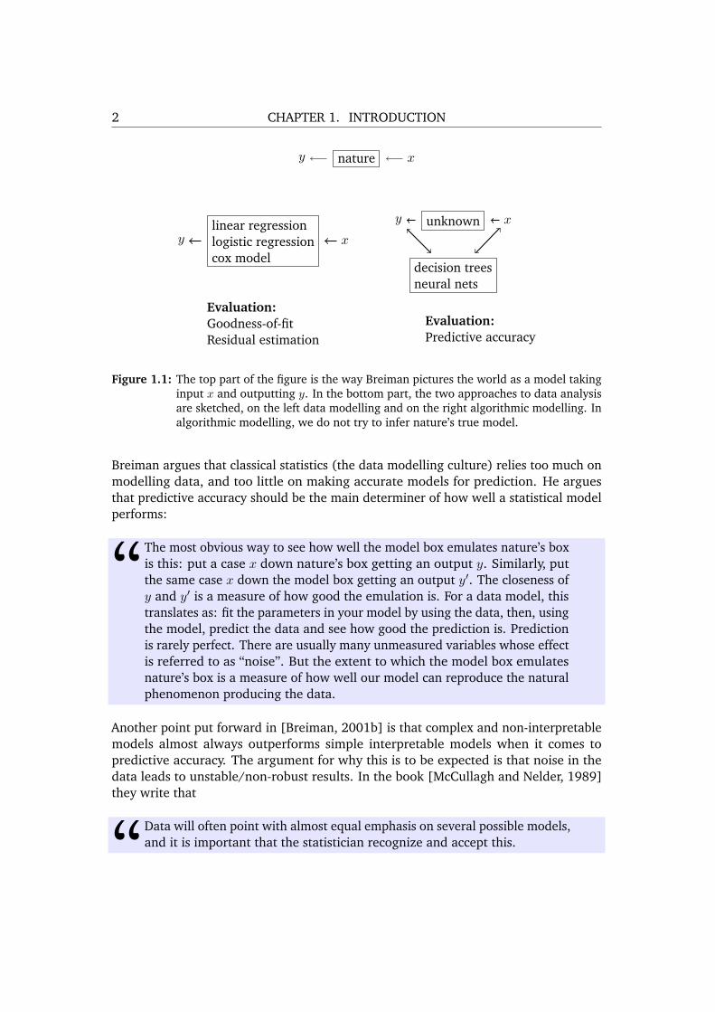
In his well-known paper “Statistical Modeling : The Two Cultures” [Breiman, 2001b],Leo Breiman divides statistical modelling into two cultures, the data modelling cultureand the algorithmic modelling culture, visualized in Figure 1.1:
1
2 CHAPTER 1. INTRODUCTION
xnaturey
xlinear regressionlogistic regressioncox model
y
Evaluation:Goodness-of-fitResidual estimation
xunknown
decision treesneural nets
y
Evaluation:Predictive accuracy
Figure 1.1: The top part of the figure is the way Breiman pictures the world as a model takinginput x and outputting y. In the bottom part, the two approaches to data analysisare sketched, on the left data modelling and on the right algorithmic modelling. Inalgorithmic modelling, we do not try to infer nature’s true model.
Breiman argues that classical statistics (the data modelling culture) relies too much onmodelling data, and too little on making accurate models for prediction. He arguesthat predictive accuracy should be the main determiner of how well a statistical modelperforms:
“ The most obvious way to see how well the model box emulates nature’s boxis this: put a case x down nature’s box getting an output y. Similarly, putthe same case x down the model box getting an output y′. The closeness ofy and y′ is a measure of how good the emulation is. For a data model, thistranslates as: fit the parameters in your model by using the data, then, usingthe model, predict the data and see how good the prediction is. Predictionis rarely perfect. There are usually many unmeasured variables whose effectis referred to as “noise”. But the extent to which the model box emulatesnature’s box is a measure of how well our model can reproduce the naturalphenomenon producing the data.
Another point put forward in [Breiman, 2001b] is that complex and non-interpretablemodels almost always outperforms simple interpretable models when it comes topredictive accuracy. The argument for why this is to be expected is that noise in thedata leads to unstable/non-robust results. In the book [McCullagh and Nelder, 1989]they write that
“ Data will often point with almost equal emphasis on several possible models,and it is important that the statistician recognize and accept this.

CONCEPTS IN PREDICTIVE MACHINE LEARNING 3
Breiman describes this effect as the Rashomon Effect:
“ Rashomon is a wonderful Japanese movie in which four people, fromdifferent vantage points, witness an incident in which one person dies andanother is supposedly raped. When they come to testify in court, they allreport the same facts, but their stories of what happened are very different.What I call the Rashomon Effect is that there is often a multitude of differentdescriptions (equations f(x)) in a class of functions giving about the sameminimum error rate.
He then argues that aggregation of simple models (also known as ensembling) leads tobetter predictions at the cost of lowering interpretability. He proceeds to give numericalevidence for this tendency by comparing a decision tree to a random forest on a numberof publicly available datasets, these results can be seen in Table 1.1.
Dataset Forest Single treeBreast cancer 2.9 5.9Ionosphere 5.5 11.2Diabetes 24.2 25.3Glass 22.0 30.4Soybean 5.7 8.6Letters 3.4 12.4Satellite 8.6 14.8Shuttle 7.0 62.0DNA 3.9 6.2Digit 6.2 17.1
Table 1.1: The test set misclassification error (%) on 10 different datasets from the UCI reposi-tory (http://archive.ics.uci.edu/ml/).
From the results shown in Table 1.1, it is clear that the complex but un-interpretablemodels achieves a lower prediction error – consequently underlining the reason fortranscending to algorithmic modelling as the core philosophy.
The arguments put forward in [Breiman, 2001b] justifies an approach to predictivemodelling where the focus is purely on predictive accuracy. That this is the right way oflooking at statistical modelling is the underlying assumption in statistical predictioncompetitions, and consequently also in this thesis.
1.2 Data prediction competitions
A recent innovation in the field of predictive modelling is the use of predictive modellingcompetitions for model selection. This concept was made popular with the NetflixPrize, a massive open competition with the aim of constructing the best algorithm

4 CHAPTER 1. INTRODUCTION
for predicting user ratings of movies. The competition featured a prize of 1,000,000dollars for the first team to improve Netflix’s own results by 10%. After the successwith the Netflix Prize, the platform Kaggle was born, providing a platform for predictivemodelling. Kaggle hosts numerous data prediction competitions and has more than150,000 users worldwide.
The basic structure of a predictive modelling competition – as seen for example onKaggle and in the Netflix competition – is the following: A predictive problem is de-scribed, and the participants are given a dataset with a number of samples and the truetarget values (the values to predict) for each sample given, this is called the trainingset. The participants are also given another dataset like the training set, but where thetarget values are not known, this is called the test set. The task of the participants isto predict the correct target values for the test set, using the training set to build theirmodels. When participants have a set of proposed predictions for the test set, they cansubmit these to a website, which will then evaluate the submission on a part of thetest set known as the quiz set, the validation set or simply as the public part of the testset. The result of this evaluation on the quiz set is shown in a leaderboard giving theparticipants an idea of how they are progressing.
Using a competitive approach to predictive modelling is being praised by some as themodern way to do science:
“ Kaggle recently hosted a bioinformatics contest, which required participantsto pick markers in a series of HIV genetic sequences that correlate with achange in viral load (a measure of the severity of infection). Within a weekand a half, the best submission had already outdone the best methods inthe scientific literature. [Goldbloom, 2010]
(Anthony Goldbloom, Founder and CEO at Kaggle)
“ These prediction contests are changing the landscape for researchers inmy area — an area that focuses on making good predictions from finite(albeit sometimes large) amount of data. In my personal opinion, they arecreating a new paradigm with distinctive advantages over how research istraditionally conducted in our field. [Mu, 2011]
(Mu Zhu, Associate Professor, University of Waterloo)
This competitive approach is interesting and seems fruitful – one can even see it as anextension of the aggregation ideas put forward in [Breiman, 2001b]. Still one shouldask if the framework provided by for example Kaggle gives a trustworthy resemblanceof real-world predictive modelling problems where problems do not come with a quizset and a leaderboard.
Thesis outline In Chapter 2 we will state and investigate a set of hypotheses aboutpredictive modelling in a competitive framework. In Chapter 3 we will outline a con-

CONCEPTS IN PREDICTIVE MACHINE LEARNING 5
ceptual framework for approaching predictive modelling competitions – from the initialdata preprocessing to final model selection and combination. This framework will bebuilt on personal experience, literature studies, interviews we did with prominent dataanalysts and on mathematical theory. Chapter 4 describes the underlying mathematicaltheory behind the models used throughout the thesis. In Chapter 5 and Chapter 6we describe two specific competitions on the Kaggle platform, our approach in thecompetitions and the results obtained. This will help validate our conceptual frameworkand will put the hypotheses to another test. Finally we conclude in Chapter 7.


Chapter 2
Hypotheses
In this chapter we state 5 hypotheses about predictive modelling in a competitiveframework. We will try to verify the validity of each hypothesis using a combinationof mathematical arguments, empirical evidence from previous competitions (gatheredin Appendix A) and qualitative interviews we did with some of the top participants atKaggle (gathered in Appendix C).
The five hypotheses to be investigated in this chapter are:
1. Feature engineering is the most important part of predictive machine learning
2. Overfitting to the leaderboard is a real issue
3. Simple models can get you very far
4. Ensembling is a winning strategy
5. Predicting the right thing is important
2.1 Feature engineering is the most important part
With the extensive amount of free tools and libraries available for data analysis, every-body has the possibility of trying advanced statistical models in a competition. As aconsequence of this, what gives you most “bang for the buck” is rarely the statisticalmethod you apply, but rather the features you apply it to.
“ For most Kaggle competitions the most important part is feature engineering,which is pretty easy to learn how to do. (Tim Salimans)
7

8 CHAPTER 2. HYPOTHESES
“ As a general rule good feature selection is what determines success ratherthan clever algorithms.
Response to question on the Kaggle Forum:http://www.kaggle.com/forums/t/5762/what-is-your-workflow/31264 (Robin East)
There are some types of data where feature engineering matters more. Examples ofsuch data types is natural language data and image data. In many of the previouscompetitions with text data and image data, feature engineering was a huge part ofthe winning solutions (examples of this are for example SUNNYHASHTAGS, FACEBOOK,SEECLICKPREDICT and BIRD).
In the competition SUNNYHASHTAGS (described in Appendix A.2) which featuredtext data taken from Twitter, feature engineering was a major part of the winningsolution. The winning solution used a simple regularized regression model (describedin Section 4.3), but generated a lot of features from the text:
“ My set of features included the basic tfidf of 1,2,3-grams and 3,5,6,7 ngrams.I used a CMU Ark Twitter dedicated tokenizer which is especially robust forprocessing tweets + it tags the words with part-of-speech tags which canbe useful to derive additional features. Additionally, my base feature setincluded features derived from sentiment dictionaries that map each wordto a positive/neutral/negative sentiment. I found this helped to predict Scategories by quite a bit. Finally, with Ridge model I found that doing anyfeature selection was only hurting the performance, so I ended up keepingall of the features ˜ 1.9 mil. The training time for a single model was stillreasonable. (aseveryn - 1st place winner)
In the competitions which did not feature text or images, feature engineering some-times still played an important role in the winning entries. An example of this is theCAUSEEFFECT competition, where the winning entry (described in Appendix A.10)created thousands of features, and then used genetic algorithms to remove non-usefulfeatures again.
On the contrary, sometimes the winning solutions are those which go a non-intuitiveway and simply use a black-box approach. An example of this is the SOLARENERGY
competition (described in Appendix A.6) where the Top-3 entries almost did not use anyfeature engineering (even though this was the intuitive approach for the competition) –and simply combined the entire dataset into one big table and used a complex black-boxmodel.

CONCEPTS IN PREDICTIVE MACHINE LEARNING 9
2.1.1 Mathematical justification for feature engineering
When using simple models, it is often necessary to engineer new features to capturethe right trends in the data. The most common example of this, is attempting to use alinear method to model non-linear behaviour.
To give a simple example of this, assume we want to predict the price of a house Hgiven the dimensions (length lH and width wH of the floor plan) of the house. Assumealso that the price p(H) can be described as a linear function p(H) = αaH + β, whereaH = lH ·wH is the area. By fitting a linear regression model to the original parameterslH , wH , we will not capture the quadratic trend in the data. If we instead construct anew feature aH = lH · wH (the area), for each data sample (house), and fit a linearregression model using this new feature, then we will be able to capture the trend weare looking for.
2.2 Simple models can get you very far
When looking through descriptions of people’s solutions after a competition has ended,there is often a surprising number of very simple solutions obtaining good results. Whatis also surprising, is that the simplest approaches are often described by some of themost prominent competitors.
“ I think beginners sometimes just start to “throw” algorithms at a problemwithout first getting to know the data. I also think that beginners sometimesalso go too-complex-too-soon. There is a view among some people thatyou are smarter if you create something really complex. I prefer to tryout simpler. I “try” to follow Albert Einstein’s advice when he said, “Anyintelligent fool can make things bigger and more complex. It takes a touchof genius – and a lot of courage – to move in the opposite direction”.
(Steve Donoho)
“ My first few submissions are usually just “baseline” submissions of extremelysimple models – like “guess the average” or “guess the average segmentedby variable X”. These are simply to establish what is possible with verysimple models. You’d be surprised that you can sometimes come very closeto the score of someone doing something very complex by just using asimple model. (Steve Donoho)
Simplicity can come in multiple forms, both regarding the complexity of the model,but also regarding the pre-processing of the data. In some competitions, regularizedregression (as described in Section 4.3) can be the winning model in spite of itssimplicity. In other cases, the winning solutions are those who do almost no pre-processing of the data (as seen in for example the SOLARENERGY competition describedin Appendix A.6).

10 CHAPTER 2. HYPOTHESES
2.3 Ensembling is a winning strategy
As described in [Breiman, 2001b], complex models and in particular models which arecombinations of many models should perform better when measured on predictiveaccuracy. This hypothesis can be backed up by looking at the winning solutions for thelatest competitions on Kaggle.
If one considers the 10 latest competitions on Kaggle (as described in Appendix A)and look at which models the top participants used, one finds that in 8 of the 10competitions, model combination and ensembling was a key part of the final submission.The only two competitions where no ensembling was used by the top participants wereFACEBOOK and BELKIN, where a possible usage of ensembling was not clear.
“ [The fact that most winning entries use ensembling] is natural from acompetitors perspective, but potentially very hurtful for Kaggle/its clients:a solution consisting of an ensemble of 1000 black box models does notgive any insight and will be extremely difficult to reproduce. This will nottranslate to real business value for the comp organizers. Also I myself thinkit is more fun to enter competitions where you actually have to think aboutyour model, rather than just combining a bunch of standard ones. In thechess rating, don’t overfit, and dark worlds competitions, for example, Iused only a single model. (Tim Salimans)
“ I am a big believer in ensembles. They do improve accuracy. BUT I usuallydo that as a very last step. I usually try to squeeze all that I can out ofcreating derived variables and using individual algorithms. After I feel like Ihave done all that I can on that front, I try out ensembles.
(Steve Donoho)
“ No matter how faithful and well tuned your individual models are, you arelikely to improve the accuracy with ensembling. Ensembling works bestwhen the individual models are less correlated. Throwing a multitude ofmediocre models into a blender can be counterproductive. Combining afew well constructed models is likely to work better. Having said that, it isalso possible to overtune an individual model to the detriment of the overallresult. The tricky part is finding the right balance. (Anil Thomas)
Besides the intuitive appeal of averaging models, one can justify ensembling mathemat-ically.
2.3.1 Mathematical justification for ensembling
To justify ensembling mathematically, we will follow the approach of [Tumer and Ghosh, 1996].We can look at a one-of-K classification problem and model the probability of input x

CONCEPTS IN PREDICTIVE MACHINE LEARNING 11
belonging to class i asfi(x) = p(ci|x) + βi + ηi(x),
where p(ci|x) is an a posteriori probability distribution of the i-th class given input x,where βi is a bias for the i-th class (which is independent of x) and where ηi(x) is theerror of the output for class i.
The Bayes optimal decision boundary is the loci of all points x? such that p(ci|x?) =maxk 6=i p(ck|x). Since fi(x) = p(ci|x) + βi + ηi(x), the obtained decision boundary x0
(found during model training/fitting) might differ from the Bayes optimal decisionboundary x? (although x0 is not the optimal decision boundary, it is still the mostlikely decision boundary given our training data). We will let b = x0 − x? denote thisdifference.
b
Optimal
boundary
Obtained
boundary
x
Figure 2.1: Two class distributions together with the optimal class boundary and an exampleof an obtained boundary. The difference between the boundaries is denoted b. Thelight shaded area is called the Bayesian error EBay and the dark shaded error iscalled the added error Eadd.
The goal of ensembling a set of models is to reduce the difference b between theobtained decision boundary and the optimal. Since x0 = b+ x? is the obtained decisionboundary, we have that:
fi(x? + b) = fj(x
? + b)
p(ci|x? + b) + βi + ηi(x? + b) = p(cj |x? + b) + βj + ηj(x
? + b)
p(ci|x? + b) + βi + ηi(x0) = p(cj |x? + b) + βj + ηj(x0).
We now assume that the posterior distributions p(ci|x) are locally monotonic aroundthe decision boundaries. This assumption is well-founded since the decision boundaries

12 CHAPTER 2. HYPOTHESES
are typically found in transition regions, where posteriors are not in their local extrema.Using this assumption, we make a linear approximation of pk(x) around x? to get:
p(ck|x? + b) ≈ p(ck|x?) + bp′(ck|x?), ∀k.
Using this approximation we get
p(ci|x?) + bp′(ci|x?) + βi + ηi(x0) = p(cj |x?) + bp′(cj |x?) + βj + ηj(x0),
and since p(ci|x?) = p(cj |x?) we get:
b(p′(cj |x?)− p′(ci|x?)) = (ηi(x0)− ηj(x0)) + (βi − βj)
b =ηi(x0)− ηj(x0)
s+βi − βjs
,
where s = p′(cj |x?)− p′(ci|x?) is the difference of the derivatives of the posteriors inthe optimal decision boundary. When fitting a model to obtain a decision boundarybetween the two classes, there is a part of the error which is due to overlap of theclasses (the so-called Bayesian error EBay) and a part of the error which is due to ourmodel-fit not being optimal (called the added error Eadd). In Figure 2.1 the dark shadedarea is the added error and the light shaded error is the Bayesian error. Since we cannot lower the Bayesian error, we can hope to lower the added error by using ensembling.
As given in [Tumer and Ghosh, 1996], when the ηk(x) are zero-mean i.i.d. one can
show that b is a zero-mean random variable with variance σ2b =
2σ2ηks2
and we can writethe added error when averaging as
Eaveadd =
s
2σ2bave ,
and we want to obtain an expression for how this depends on the number of models inthe ensemble. Say we fit N models, and let fave
i be their average, then we have
favei =
1
N
N∑m=1
f(m)i (x) = p(ci|x) + βi + ηi(x),
where βi = 1N
∑Nm=1 β
(m)i and ηi(x) = 1
N
∑Nm=1 η
(m)i (x). This is due to the fact that the
true posterior probability distribution p(ci|x) is the same for all model fits. Now thevariance of ηi = 1
N
∑Nm=1 η
(m)i is given by
σ2ηi =
1
N2
N∑l=1
N∑m=1
cov(η
(m)i (x), η
(l)i (x)
)=
1
N2
N∑m=1
σ2
η(m)i (x)
+1
N2
N∑m=1
∑l 6=m
cov(η
(m)i (x), η
(l)i (x)
),

CONCEPTS IN PREDICTIVE MACHINE LEARNING 13
since we have that cov(x, x) = var(x). Using the fact that cov(x, y) = corr(x, y)σxσywe get that
σ2ηi =
1
N2
N∑m=1
σ2
η(m)i (x)
+1
N2
N∑m=1
∑l 6=m
corr(η
(m)i (x), η
(l)i (x)
)ση(m)i (x)
ση(l)i (x)
.
Using the common variance σ2ηi(x) which is the average over the m models and the
average correlation factor δi defined as
δi =1
N(N − 1)
N∑m=1
∑m 6=l
corr(η
(m)i (x), η
(l)i (x)
),
we can get
σ2ηi =
1
Nσ2ηi(x) +
N − 1
Nδiσ
2ηi(x).
If we look at the decision boundary offset b of two classes i and j (see Figure 2.1), weget that the variance of b averaged over the N models is given by
σ2bave = Var
(ηi(x0)− ηj(x0)
s+βi − βjs
)= Var
(ηi(x0)− ηj(x0)
s
)=σ2ηi + σ2
ηj
s2.
Consequently we get that
σ2bave =
σ2ηi(x) + σ2
ηj(x)
Ns2+N − 1
Ns2
(δiσ
2ηi(x) + δjσ
2ηj(x)
).
Now we use that the noise (η) between classes is identically and independently dis-tributed and the fact that
σ2ηi(x) + σ2
ηj(x)
s2= σ2
b ,
to obtain
σ2bave =
1
Nσ2b +
N − 1
Ns2
(δiσ
2ηi(x) + δjσ
2ηj(x)
)=
1
Nσ2b +
N − 1
N
2δiσ2ηi(x)
s2
δjσ2ηj
2
=σ2b
N
(1 + (N − 1)
δi + δj2
).
We now introduce δ =∑K
i=1 Piδi where Pi is the prior probability of class i. Thecorrelation contribution of each class to the overall correlation is proportional to theclass prior probability. Using this and the fact that Eadd = s
2σ2b , we get that
Eaveadd =
s
2σ2bave =
s
2σ2b
(1 + δ(N − 1)
N
)= Eadd
(1 + δ(N − 1)
N
).
14 CHAPTER 2. HYPOTHESES
Looking at the above formula, we observe that a correlation of δ = 0 (i.e. no correlation)will make Eave
add = EaddN and that δ = 1 (i.e. total correlation) will make Eave
add = Eadd.
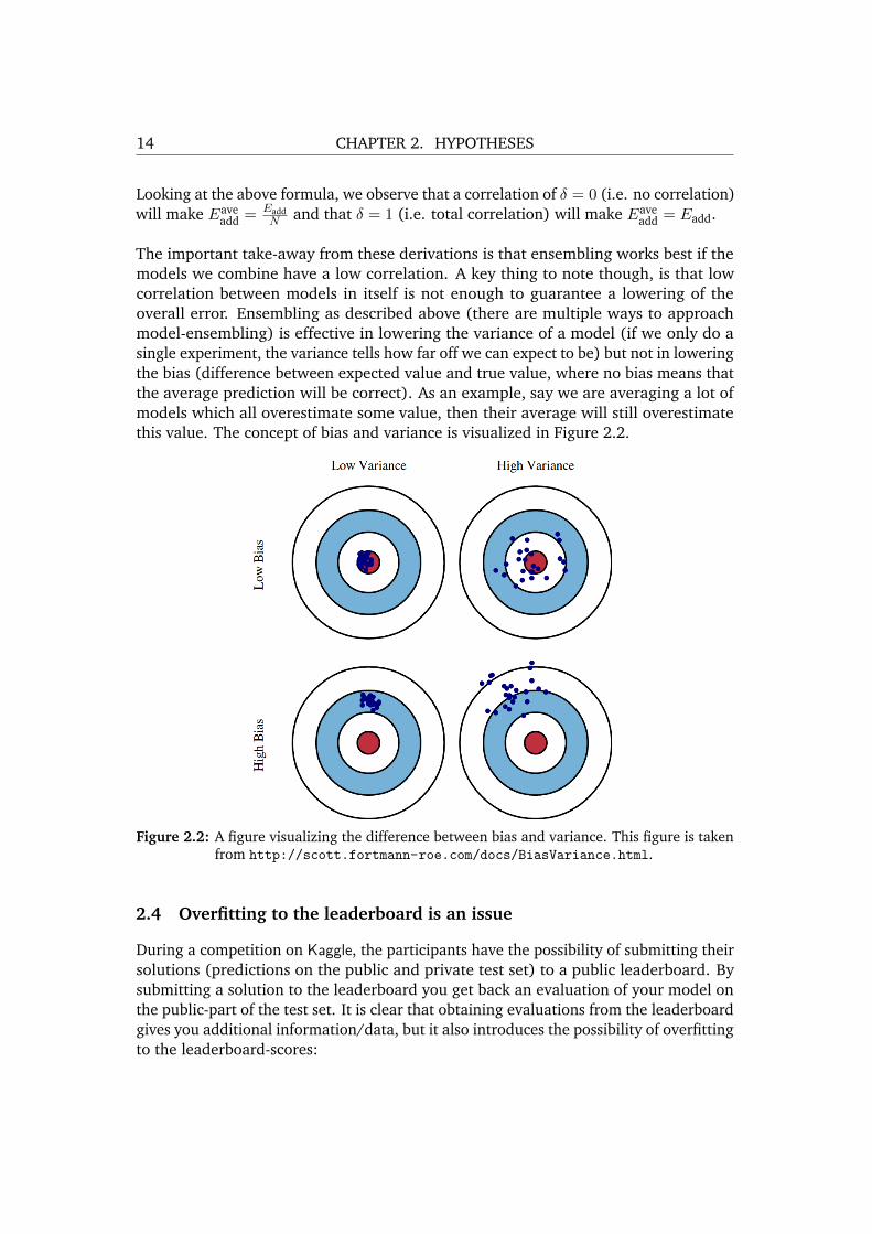
The important take-away from these derivations is that ensembling works best if themodels we combine have a low correlation. A key thing to note though, is that lowcorrelation between models in itself is not enough to guarantee a lowering of theoverall error. Ensembling as described above (there are multiple ways to approachmodel-ensembling) is effective in lowering the variance of a model (if we only do asingle experiment, the variance tells how far off we can expect to be) but not in loweringthe bias (difference between expected value and true value, where no bias means thatthe average prediction will be correct). As an example, say we are averaging a lot ofmodels which all overestimate some value, then their average will still overestimatethis value. The concept of bias and variance is visualized in Figure 2.2.
Figure 2.2: A figure visualizing the difference between bias and variance. This figure is takenfrom http://scott.fortmann-roe.com/docs/BiasVariance.html.
2.4 Overfitting to the leaderboard is an issue
During a competition on Kaggle, the participants have the possibility of submitting theirsolutions (predictions on the public and private test set) to a public leaderboard. Bysubmitting a solution to the leaderboard you get back an evaluation of your model onthe public-part of the test set. It is clear that obtaining evaluations from the leaderboardgives you additional information/data, but it also introduces the possibility of overfittingto the leaderboard-scores:

CONCEPTS IN PREDICTIVE MACHINE LEARNING 15
“ The leaderboard definitely contains information. Especially when the leader-board has data from a different time period than the training data (such aswith the heritage health prize). You can use this information to do modelselection and hyperparameter tuning. (Tim Salimans)
“ The public leaderboard is some help, [...] but one needs to be careful to notoverfit to it especially on small datasets. Some masters I have talked to picktheir final submission based on a weighted average of their leaderboardscore and their CV score (weighted by data size). Kaggle makes the dangersof overfit painfully real. There is nothing quite like moving from a goodrank on the public leaderboard to a bad rank on the private leaderboard toteach a person to be extra, extra careful to not overfit. (Steve Donoho)
“ Having a good cross validation system by and large makes it unnecessaryto use feedback from the leaderboard. It also helps to avoid the trap ofoverfitting to the public leaderboard. (Anil Thomas)
In the 10 last competitions on Kaggle, 2 of them showed extreme cases of overfittingand 4 showed mild cases of overfitting. The two extreme cases were the “Big DataCombine” and “StumbleUpon Evergreen Classification Challenge”. In Tables 2.1 and 2.2the Top-10 submissions on the public test set is shown, together with the results of thesame participants on the private test set.
Name # Public # Private Public score Private score EntriesJared Huling 1 283 0.89776 0.87966 65Yevgeniy 2 7 0.89649 0.88715 63Attila Balogh 3 231 0.89468 0.88138 137Abhishek 4 6 0.89447 0.88760 90Issam Laradji 5 9 0.89378 0.88690 44Ankush Shah 6 11 0.89377 0.88676 32Grothendieck 7 50 0.89304 0.88295 73Thakur Raj Anand 8 247 0.89271 0.88086 37Manuel Dıaz 9 316 0.89230 0.87695 93Juventino 10 27 0.89220 0.88472 16
Table 2.1: Results of the Top-10 participants on the leaderboard for the competition: “Stumble-Upon Evergreen Classification Challenge”

16 CHAPTER 2. HYPOTHESES
Name # Public # Private Public score Private score EntriesKonstantin Sofiyuk 1 378 0.40368 0.43624 33Ambakhof 2 290 0.40389 0.42748 159SY 3 2 0.40820 0.42331 162Giovanni 4 330 0.40861 0.42893 215asdf 5 369 0.41078 0.43364 80dynamic24 6 304 0.41085 0.42782 115Zoey 7 205 0.41220 0.42605 114GKHI 8 288 0.41225 0.42746 191Jason Sumpter 9 380 0.41262 0.44014 93Vikas 10 382 0.41264 0.44276 90
Table 2.2: Results of the Top-10 participants on the leaderboard for the competition: “Big DataCombine”
In the “StumbleUpon Evergreen Classification Challenge” competition, the training dataconsisted of 7395 samples, and it was generally observed that the data was very noisy1.
In the “Big Data Combine” competition, the task was to predict the value of stocksmultiple hours into the future, which is generally thought to be extremely difficult2. The extreme jumps on the leaderboard is most likely due to the sheer difficulty ofpredicting stocks combined with overfitting.
In the cases where there were small differences between the public leaderboard andthe private leaderboard, the discrepancy could also be explained by scores for the topcompetitors being so close that random noise affected the positions.
Based on empirical evidence, interviews with prominent Kaggler’s and on general theoryof overfitting, it seems clear that one should think of approaches to avoid overfitting tothe leaderboard. Methods to avoid overfitting are described in Section 3.6.
2.5 Predicting the right thing is important
One subject that is sometimes extremely relevant, and other times is not relevant at all,is that of “predicting the right thing”. It seems quite trivial to state that it is importantto predict the right thing, but it is not always a simple matter.
“ A next step is to ask, “What should I actually be predicting?”. This is animportant step that is often missed by many – they just throw the rawdependent variable into their favorite algorithm and hope for the best. Butsometimes you want to create a derived dependent variable. I’ll use the GE
1http://www.kaggle.com/c/stumbleupon/forums/t/6185/what-is-up-with-the-final-leaderboard2This is what is known as the Efficient Market Hypothesis.

CONCEPTS IN PREDICTIVE MACHINE LEARNING 17
Flightquest as an example – you don’t want to predict the actual time theairplane will land; you want to predict the length of the flight; and maybethe best way to do that is to use that ratio of how long the flight actuallywas to how long it was originally estimate to be and then multiply thattimes the original estimate. (Steve Donoho)
There are two ways to address the problem of predicting the right thing: The first wayis the one addressed in the quote from Steve Donoho, about predicting the correctderived variable. The other is to train the statistical models using the appropriate lossfunction. This issue was addressed in the forum of the SOLARENERGY competition:
“ Did anyone achieve a “good” score using RandomForest?- Abhishek
I don’t think so. Most RF implementations targets MSE, and the metric ofthis competition is MAE, so i don’t think it will give good results.- Leustagos (1st place winner)
As an example of why using the wrong loss function might give rise to issues, lookat the following simple example: Say you want to fit the simplest possible regressionmodel, namely just an intercept a to the data:
x = (0.1, 0.2, 0.4, 0.2, 0.2, 0.1, 0.3, 0.2, 0.3, 0.1, 100)
If we let aMSE denote the a minimizing the mean squared error, and let aMAE denotethe a minimizing the mean absolute error, we get the following
aMSE ≈ 9.2818, aMAE ≈ 0.2000
If we now compute the MSE and MAE using both estimates of a, we get the followingresults:
1
11
∑i
|xi − aMAE| = 9.5909,1
11
∑i
|xi − aMSE| = 16.4942
1
11
∑i
(xi − aMAE)2 = 905.4660,1
11
∑i
(xi − aMSE)2 = 822.9869
We see (as expected) that for each loss function (MAE and MSE), the parameter whichwas fitted to minimize that loss function achieves a lower error. This should come as nosurprise, but when the loss functions and statistical methods become very complicated,it is not always as trivial to see if one is actually optimizing the correct thing.


Chapter 3
A Framework for Predictive Modelling
In this chapter we will outline a conceptual framework for approaching predictivemodelling competitions – from the initial data exploration and preprocessing to finalmodel selection and combination. For each part of the framework, we will try todescribe common methods, tricks and things to consider.
3.1 Overview
In a general setting, the process of predictive modelling in a competitive frameworkoften follows the steps shown here:
1. Explore the data
2. Clean/process the data
3. Construct a statistical model (repeat)
Construct features
Train model
Evaluate model
4. Select best model
“ I learned about the importance of iterating quickly. And trying out manydifferent things and validating, rather than trying to guess the best solutionbeforehand. (Tim Salimans)
In the following sections we will dive into each of these steps.
19

20 CHAPTER 3. A FRAMEWORK FOR PREDICTIVE MODELLING
3.2 Exploratory analysis
The first step when doing data analysis, should always be to explore and understandthe data. Sometimes the data is rather simple and manageable, but sometimes dataexploration can be very time consuming.
“ I start by simply familiarizing myself with the data. I plot histograms andscatter plots of the various variables and see how they are correlated withthe dependent variable. I sometimes run an algorithm like GBM [gradientboosting machine] or randomForest on all the variables simply to get aranking of variable importance. I usually start very simple and work myway toward more complex if necessary. (Steve Donoho)
“ Initially If there are continuous variables I would start by getting simplystatistics (range, mean, etc) and then plot each one against the dependentvariable. If there are categorical variables then histograms. (Robin East)
There is no perfect recipe for how to perform an adequate exploratory analysis, it isa matter of experience and hard work. Still, there are some things which are often agood idea to consider when exploring the data.
3.2.1 Outlier detection
An important reason for exploring the data is to see if there is “wrong” data in theprovided dataset. This can be measurements which violates some kind of assumption.In our recent work with data analysis competitions, some of the things which havecome up in this category are: Probabilities not summing to one, products which aresent for repair before even being sold and hotel prices of a million dollars per night.
The best way to find outliers, is to either inspect the minimum value, the maximumvalue and the percentiles of the data numerically, or more commonly to make plots ofthe different variables.
3.2.2 Plotting the data
One of the best ways to explore data is to visualize it. If one has thousands or maybeeven millions of data samples, exploring them manually is not a real possibility. Usingthe right kinds of visualizations can give the insight into the data which is needed. Thereis a vast amount of literature and research on how to make good data visualizations, sowe will simply mention some of the most common and trivial ones here. We will use adataset of flowers (the well known iris dataset) for examples.
The most common and simple plot is the scatter plot as shown in Figure 3.1. It showsthe relation between two numerical variables using points.

CONCEPTS IN PREDICTIVE MACHINE LEARNING 21
●●●
●●
●
●●
●● ●
●
●
●●
●
●●
●
●
●
●
●
●
●
● ●●
●
●●● ●
●●
●●
●●
●
●● ●
●
●
●
●
●●
●
●
●
●
●
●●
●
●
●
●
●
●
●
●
●
●●
●
●
●
●
●
●
●
●●
●
●
●
●
●●
●
●
● ●
●
●
●●
●
●
●
●
● ●●●
●
●
●
●
●
●
●
●
●
●
●
●
●
●
●
●●
●
●
●
●
●
●
●
●
●
●
●
●●
●
●
●
●
●
●
●
●
●●
●
●
●
●●
●
●
●
●
●
●
●
2
4
6
2.0 2.5 3.0 3.5 4.0 4.5Sepal.Width
Pet
al.L
engt
h
●●●
●●
●
●●
●● ●●
●
● ●
●
●●
●●
●●
●
●
●
● ●●●
●●● ●
●●
●●
●●
●
●● ●
●
●
●
●
● ●●
●
●
●
●
●●
●
●
●
●
●
●
●
●
●
●●
●
●
●
●
●
●
●
●●
●●
●
●
●●
●
●
● ●
●
●
●●
●
●
●
●
● ●●●
●
●
●
●
●
●
●
●
●
●
●
●
●
●●
●●
●●
●
●
●
●
●
●
●
●
●
●●
●●
●
●
●
●
●
●
●●
●
●
●
●●
●
●
●
●
●●
●
2
4
6
2.0 2.5 3.0 3.5 4.0 4.5Sepal.Width
Pet
al.L
engt
h
Figure 3.1: Two scatter plots showing the connection between the sepal width and the petallength. In the scatter plot on the right, colors have been added to show the differentspecies of Iris, and a bit of random noise have been added to the points to avoidthem being exactly on top of each other.
Using histograms as shown in Figure 3.2, one can visualize a single variable. Valuesclose to each other are combined in bins, and the height of the bins indicate the numberof samples binned together.
0
5
10
4 5 6 7 8Sepal.Length
coun
t
0.0
2.5
5.0
7.5
4 5 6 7 8Sepal.Length
coun
t
Species
setosa
versicolor
virginica
Figure 3.2: Two histograms showing the distribution of sepal length. In the right histogram,the different Iris species are shown with different colors, making it clear that thesepal length differs between species.
Another way to visualize a single variable is to use box-plots as shown in Figure 3.3.Normally, box-plots show the minimum value, maximum value, the lower and upperquartiles and the median in one graphic.

22 CHAPTER 3. A FRAMEWORK FOR PREDICTIVE MODELLING
●
●
●
●
●
●
●
●
●
●
●
●●
●
●
●
●
●●
●
●
●
●
●●
●
●●
●
●
●
●
●
●
●
●
●
●
●
●
●
●●
●
●●
●
●
●
●
●
●
●
●
●
●●
●
●
● ●
●
●
●
●
●
●
●
●●
●
●
●
●
●
●
●
●
●
●●
●
●
●
●
●●
●●
●
●
●
●
●
●
●
●
●
●
●
●
●●
●
●
●
●
●
●●●
●
●
●
●
●
●
●
●
●
●
●
●
●
●
●
●●
●
●
●
●
●
●
●
●
●
●●
●
●
●
●
●
●●●
●
●●
●
●
●
●
●
2.0
2.5
3.0
3.5
4.0
4.5
setosa versicolor virginicaSpecies
Sep
al.W
idth Species
●
●
●
setosa
versicolor
virginica
Figure 3.3: A box plot of the sepal width for the three different species. On top of the boxplot, the actual data is shown with some horizontal noise added to make all pointsvisible.
3.2.3 Variable correlations
Another thing which is common to explore, is correlations between variables. If thereare features which are very correlated, it might be possible to remove some of them toreduce the number of features. If some of the features are correlated with the targetvalues, then those features will have significance when making predictions. A way tovisually inspect correlations between features is using correlation matrix-plots as shownin Figure 3.4.

CONCEPTS IN PREDICTIVE MACHINE LEARNING 23
Sepal.Length
2.0 2.5 3.0 3.5 4.0
0.12 0.87
0.5 1.0 1.5 2.0 2.5
4.5
5.0
5.5
6.0
6.5
7.0
7.5
8.0
0.82
2.0
2.5
3.0
3.5
4.0
●
●
●
●
●
●
● ●
●
●
●
●
●●
●
●
●
●
●●
●
●
●
●
●
●
●
●
●
●
●
●
●
●
●
●
●
●
●
●
●
●
●
●
●
●
●
●
●
●
●●
●
●
●●
●
●
●
●
●
●
●
●●
●
●
●
●
●
●
●
●
●
●
●
●
●
●
●
●●
● ●
●
●
●
●
●
●
●
●
●
●
●
●
● ●
●
●
●
●
●
●
● ●
●
●
●
●
●
●
●
●
●
●
●
●
●
●
●
● ●
●
●
●
●
●
●
●
●
●
●●
●
●
●
●
●
●● ●
●
●
●
●
●
●
●
●
Sepal.Width 0.43 0.37
●●●
●●
●
●●
●● ●
●
●
●●
●
●●
●
●
●
●
●
●
●
●●●●
● ●●●
●●
●●
●●
●
●●●
●
●
●
●
●●
●
●
●
●
●
●●
●
●
●
●
●
●
●
●
●
●●
●
●
●
●
●
●
●
●●
●
●
●
●
●●
●
●
● ●
●
●
●●
●
●
●
●
● ●●●
●
●
●
●
●
●
●
●
●
●
●
●
●
●
●
●●
●
●
●
●
●
●
●
●
●
●
●
●●
●
●
●
●
●
●
●
●
●●
●
●
●
●●
●
●
●
●
●
●
●
●●●
●●
●
●●
●● ●
●
●
●●
●
●●
●
●
●
●
●
●
●
● ●●
●
●●● ●
●●
●●
●●
●
●● ●
●
●
●
●
●●
●
●
●
●
●
●●
●
●
●
●
●
●
●
●
●
●●
●
●
●
●
●
●
●
●●
●
●
●
●
●●
●
●
● ●
●
●
●●
●
●
●
●
● ●●●
●
●
●
●
●
●
●
●
●
●
●
●
●
●
●
●●
●
●
●
●
●
●
●
●
●
●
●
●●
●
●
●
●
●
●
●
●
●●
●
●
●
●●
●
●
●
●
●
●
●
Petal.Length
12
34
56
7
0.96
4.5 5.0 5.5 6.0 6.5 7.0 7.5 8.0
0.5
1.0
1.5
2.0
2.5
●●●● ●
●
●
●●
●
●●
●●
●
●●
● ●●
●
●
●
●
● ●
●
●●● ●
●
●
●● ● ●
●
● ●
●●
●
●
●
●
●● ●●
●
● ●
●
●
●
●
●
●
●
●
●
●
●
●
●
●
●
●
●
●
●
●
●
●
● ●
●
●
●
●
●
●
●
●
●
●
●●●
●
●
●
●
●
●
● ●
●
●
●
●
●
●
●
●
●
●●
●
●
●
●
●
●
●
●
●
●
●
●
● ●
●
●
●●●
●
●
●
●
●
●
●
●
●
●●
●
●
●
●
●
●
●
●
●
●
●
●● ●● ●
●
●
●●
●
●●
●●
●
●●
● ●●
●
●
●
●
●●
●
●●●●
●
●
●● ● ●
●
● ●
●●
●
●
●
●
●● ●●
●
●●
●
●
●
●
●
●
●
●
●
●
●
●
●
●
●
●
●
●
●
●
●
●
●●
●
●
●
●
●
●
●
●
●
●
● ●●
●
●
●
●
●
●
●●
●
●
●
●
●
●
●
●
●
●●
●
●
●
●
●
●
●
●
●
●
●
●
●●
●
●
●● ●
●
●
●
●
●
●
●
●
●
●●
●
●
●
●
●
●
●
●
●
●
●
1 2 3 4 5 6 7
●●● ●●
●
●
●●
●
●●
●●
●
●●
● ●●
●
●
●
●
●●
●
●● ●●
●
●
●●●●
●
● ●
●●
●
●
●
●
●●●●
●
● ●
●
●
●
●
●
●
●
●
●
●
●
●
●
●
●
●
●
●
●
●
●
●
● ●
●
●
●
●
●
●
●
●
●
●
●●●
●
●
●
●
●
●
●●
●
●
●
●
●
●
●
●
●
●●
●
●
●
●
●
●
●
●
●
●
●
●
● ●
●
●
●●●
●
●
●
●
●
●
●
●
●
●●
●
●
●
●
●
●
●
●
●
●
●
Petal.Width
Iris Scatterplot Matrix
Figure 3.4: A variable correlation matrix-plot. In the diagonal of the matrix, the variable nameis stated. In the lower triangular part of the matrix, scatter plots are shown foreach pair of variables, including a smoothed curve showing the trend in the data.In the upper triangular part of the matrix, the correlation coefficients are shown,with sizes relative to the amount of correlation.
3.3 Data preparation
It is often stated that around 80%–90% of the time spent on doing data analysis isspent on the process of cleaning and preparing the data [Dasu and Johnson, 2003].

24 CHAPTER 3. A FRAMEWORK FOR PREDICTIVE MODELLING
“ Depending on the competition, data preparation can take up a lot of time.For some contests, the data is fairly simple – one flat table – and a user canstart applying learning algorithms right away. For other contests – the GEFlightquest contests are an example – there is a lot of data prep work beforeone can even begin to apply learning algorithms. (Steve Donoho)
One common way to structure data is to use the so-called tidy-data format [Wickham, 2012]:
1. Each variable forms a column
2. Each observation forms a row
3. Each table/file stores data about one kind of observation
Other things which should hold for cleaned data are
1. Column names are easy to use and informative
2. Row names are easy to use and informative
3. Obvious mistakes in the data should be removed
4. Variable values are internally consistent
5. Appropriate transformed variables have been added
The paper [Wickham, 2012] describes a consistent way to tidy up data for analysis.According to [Leek, 2013], some of the most important steps to take when doing datapreparation is
1. Fix variable names
2. Create new variables
3. Merge datasets
4. Reshape datasets
5. Deal with missing data
6. Take transforms of variables
7. Check on and remove inconsistent values
Since no two datasets are alike, there is not a right way to prepare the data, it is asmuch a matter of personal preferences as of using the right approach for the specificproblem.

CONCEPTS IN PREDICTIVE MACHINE LEARNING 25
3.3.1 Tools for data analysis
There are many tools for doing data analysis, some of them – for example MATLABand Python – have a very broad focus whereas others like R, are more specialized. Eachtool has its own advantages and disadvantages, so it is common for people to employmultiple tools when doing their data analysis.
Here we will attempt to give a short description of the pros and cons of 3 of the maintools1.
R
One of the most widely used tools for data analysis is R. It is a free software packagewith a big user base and a large repository of freely available packages implementingmost statistical methods and models.
R is based on the S-language and is focused towards more classical statistics. R is verygood for doing exploratory data analysis, plotting graphics and handling dirty data(combinations of data types, missing values and generally data not in a matrix format).
Currently, the main problem with R is efficiency, both regarding speed but especiallymemory.
MATLAB
Within the machine learning and applied mathematics community, a very common toolis MATLAB. MATLAB is a non-free (although the open source clone Octave is available)suite of tools for numerical computing.
The strength of MATLAB is in its abilities to effectively handle matrices (MATLAB is anabbreviation of Matrix Laboratory) and its wide range of toolboxes for optimization,image analysis and statistics.
The biggest issues with MATLAB are efficiency, and its lacking focus on handling dirtydata – but when the data is structured as simple matrices (or tensors in general), it ishighly efficient.
Python
Recently, Python is becoming more popular in the machine learning community. Es-pecially packages such as scikit-learn2 and pandas3 have sparked the interest for using
1This description will be somewhat biased, but is also heavily based on online debates about the issue.2http://scikit-learn.org/stable/3http://pandas.pydata.org/

26 CHAPTER 3. A FRAMEWORK FOR PREDICTIVE MODELLING
Julia Python R MATLABfib 0.91 30.37 411.36 1992.00parse int 1.60 13.95 59.40 1463.16quicksort 1.14 31.98 524.29 101.84mandel 0.85 14.19 106.97 64.58pi sum 1.00 16.33 15.42 1.29rand mat stat 1.66 13.52 10.84 6.61rand mat mul 1.01 3.41 3.98 1.10
Table 3.1: Benchmark times relative to C (smaller is better, C performance = 1.0). Thesebenchmarks and descriptions are given on http://julialang.org/ and include otherlanguages as well.
Python as a tool for data analysis.
One of the main reasons for using Python when doing data analysis, is that Pythonis built to be an entire programming language by itself – meaning that you can uselanguage features such as object oriented programming to build and structure entireanalysis pipelines. Another reason for using Python for data analysis is its efficiency(speed and memory) compared to R and MATLAB.
While the fact that Python is built to be an entire programming language is sometimesan advantage, it is also the main concern with using Python for data analysis. Toolslike R are built specifically to be used for data analysis, sometimes making the use ofPython for data analysis a less wholesome experience.
Julia
In the future, the modelling language of choice might be Julia4, promising syntax likeMATLAB, speed like C and plotting facilities like R. Table 3.1 shows a comparison ofspeed for C, R, MATLAB, Python and Julia.
3.3.2 Large datasets
In some competitions the dataset provided is large. When talking about large datahere, we mean that the data is too big to fit in memory on a common computer.Either the data in its original form is too large to fit in memory, or the data afternecessary pre-processing and feature expansion is too big. Examples of competitionswith large datasets are FACEBOOK, SUNNYHASHTAGS, SEECLICKPREDICT, ACCELEROME-TER, STUMBLEUPON and BELKIN. Of these competitions, FACEBOOK, SUNNYHASHTAGS,SEECLICKPREDICT and STUMBLEUPON features mainly text-data, where the commonfeature generation/expansions gives rise to a very large dataset, and BELKIN features a
4http://julialang.org/

CONCEPTS IN PREDICTIVE MACHINE LEARNING 27
large dataset of images which by nature are very high-dimensional.
One way to approach very large datasets is the use of special data structures. Anexample of this is sparse matrices, which are matrices where only non-zero elementsare stored. Sparse matrices are very common for natural language processing tasks,where one usually has a huge number of very sparse features. The down-fall of usingsparse matrices, is that common operations such as look-up becomes much more timeconsuming. MATLAB features good implementations of sparse matrices and algorithmson them.
Another way to structure data of large size is using classical relational databases suchas MySQL and PostgreSQL. Relational databases stored on disk, scale without problemsand features fast look-ups and aggregations. The main issue with using databases isthat most of the statistical models will not work out of the box as with data in tableformat.
Finally, when the data becomes too big, training complex models is simply not feasible.In this case, the most common approach will be to hand-code aggregated features.An example of this is the winning entry of the FACEBOOK competition described inAppendix A.1.2.
Specialized tools for large datasets
In the last years, a lot of research focus has been put on building models, software andconceptual approaches to handle large datasets.
An example of a conceptual approach is the MapReduce framework, with the most popu-lar implementation thereof being Apache Hadoop. MapReduce reduces all computationsinto two steps, a map-step and a reduce step. In the map-step, the master node dividesthe input into smaller sub-problems which are then distributed to worker-nodes (thismight be done recursively). In the reduce-step, the master node collects the answersfrom worker nodes and combines them. The advantage of formulating computationsusing the MapReduce framework is that it enables parallel processing of data. Not allproblems can be parallelized easily, but when it is possible, a large speed-up is achieved.
An example of software built for large datasets is Vowpal Wabbit5, self-described as:
“ VW is the essence of speed in machine learning, able to learn from terafea-ture datasets with ease. Via parallel learning, it can exceed the throughputof any single machine network interface when doing linear learning, a firstamongst learning algorithms.
5http://hunch.net/˜vw/

28 CHAPTER 3. A FRAMEWORK FOR PREDICTIVE MODELLING
Vowpal Wabbit is an extremely efficient implementation of different learning algorithms,for example:
• Ordinary Least Squares Regression
• Matrix Factorization
• Neural Networks
• Latent Dirichlet Allocation
and has implementations of different types of regularization and the possibility tohandle text-data directly.
3.4 Feature engineering
As discussed in Section 2.1, predictive analysis is all about having the correct features.In some situations, there are no directly useful features (like in image analysis) and inother situations there is a vast amount of irrelevant or correlated features.
In this section we will try to describe some of the common techniques for handlingfeature-related issues in predictive analysis. We will split the section into two parts, oneabout reducing the number of features (by removing the least useful features), and oneabout generating and extracting new useful features.
3.4.1 Feature reduction
A simple and yet very effective way to reduce the number of features, is to manuallyremove some of them based on intuition about their importance. As an example, sayyou want to predict the value in dollars for which a product is sold on an online auction(like eBay). Assume that you are given a lot of meta-data about the product, includingthe time when the item (year, month, date, hour, minute and second) was posted onthe website. It is not possible to exclude the possibility that the variables year, month,date and hour could have an important effect on the price (for example, prices mightbe higher around Christmas time). On the other hand, the second which the productwas posted does most likely not hold any information about the sale price. Removingnon-useful features will make the statistical models simpler, more robust and less proneto overfitting.
Sometimes the number of features is very large, and it is not always intuitive whichfeatures hold predictive power. In this case, we can apply automatic methods forremoving non-useful features. Three such methods are stepwise regression, Lasso (de-scribed in Section 4.3) and using advanced models such as random forests (described inSection 4.1).

CONCEPTS IN PREDICTIVE MACHINE LEARNING 29
Stepwise regression is regression, where the variables are either introduced gradually,or removed gradually. For simplicity, we will just describe the first type, namely forwardselection. In forward selection, the initial regression model includes no variables. Theneach possible variable is added, and the model fit is evaluated (using some criterion,such as a t-test or the r2 value). The variable which gives the biggest gain in model fitis put into the model, and the procedure is continued until some criteria is met. Thereare multiple issues with stepwise regression, the main one being that the same data isbeing used for model-training and evaluation [Rencher and Pun, 1980].
A more advanced (and very popular) approach to feature reduction is to use forexample random forests (or other complex methods) for selecting features. For thisexplanation, we will assume that the reader has the knowledge of random forestspresented in Section 4.1. The basic idea behind using random forests to measurevariable importance is the following: A random forest is fitted to the data, and the out-of-bag error measure is calculated. To measure the importance of feature j, we permutethe values in feature j and compute the out-of-bag error again on this permuted dataset.If the out-of-bag estimate increases a lot by permuting feature j, then that featuremust have been important for the predictions. Consequently we rank the featuresby the difference in out-of-bag error we get by permuting them, normalized in anappropriate way. There are some technicalities regarding categorical variables withdifferent number of categories, which can be solved using so-called partial permutationsas described in [Deng et al., 2011].
3.4.2 Feature generation and extraction
In many cases, the given features are not directly useful or are very correlated. Oneexample of features that are not directly useful is the one described in Section 2.1.1where we wanted to predict the price of a house by its width and length (instead of thearea). Another example is in image analysis tasks, where the original features (pixelintensities) are not directly useful (in simple models). In other situations, the featuresare many and highly correlated, making it hard to fit robust statistical models. In thiscase, one can try to replace the features by a new and smaller set of “better” features,holding the same information as the original features.
Basis expansions
Generating new features as non-linear combinations of the original features is calledbasis expansion. Given a set of features x1, x2, . . ., common new features to generateare
xixj , x2i , log xi,
√xi
Often, relevant basis expansions can be done manually, as in the house example (seeSection 2.1.1) where we create a feature area by multiplying features width and length.

30 CHAPTER 3. A FRAMEWORK FOR PREDICTIVE MODELLING
Expansion of categorical features
Often features are not numerical values but categorical, for example which brand acar has or which country a person is from. In this case, it is not meaningful to use thisfeature directly in for example a linear regression model. One approach to workingwith categorical features is to expand them into multiple boolean features. Say we havea dataset of cars where one feature is the brand of the cars and where the possiblevalues are “Ford”, “Audi” and “Volvo”:
. . . Brand . . .
FordFordVolvoAudiVolvo
Now we can expand this feature into three new features, one for each possible value ofthe original feature:
. . . Ford Audi Volvo . . .
1 0 01 0 00 0 10 1 00 0 1
With the expanded feature, it is now straightforward to apply for example a linearregression model. The problem with expanding features in this way is that the numberof features can expand very rapidly if the categorical features have many categories(although one will often obtain very sparse features).
Text features
In many competitions on Kaggle, the data to be analyzed is text data, either in the formof natural language, webpages or for example tweets from Twitter. When analyzingtext data, the task of extracting features is very important since the raw text data ishard to fit into a statistical model out of the box. Common ways to extract features, isto use so-called bag-of-words, n-grams and tf-idf.
The idea behind bag-of-words, is to disregard grammar and order in the text data, butsimply storing multiplicity. Say we have the sentence6:
John likes to watch movies. Mary likes too.6Example taken from http://en.wikipedia.org/wiki/Bag-of-words model on the 2nd of February 2014.

CONCEPTS IN PREDICTIVE MACHINE LEARNING 31
Then we can represent that string as a vector (1, 2, 1, 1, 1, 1, 1) where the 7 features are:john, likes, to, watch, movies, mary, too. Note that we have a 2 since the word “likes” isused twice in the sentence. By converting a dataset of text using bag-of-words, one getsa data-matrix with a sample per document, and a feature for each unique word in theentire dataset (consequently giving a very high-dimensional – yet often very sparse –dataset).
Sometimes the context is lost when only considering words by themselves. A commonapproach to handling this issue is using n-grams which is a generalization of bag-of-words. An n-gram is a vector of n consecutive words in a text. For example, the seven2-grams (also called bi-grams) in the above text are:
{john, likes}, {likes, to}, {to, watch}, {watch, movies}
{movies, mary}, {mary, likes}, {likes, too}and now these bi-grams can be used as features as well.
Finally, another very common way of handling text data, is to use the so-called termfrequency - inverse document frequency (tf-idf) weighting scheme. The basic idea in tf-idfis to down-weight words which are very common in the dataset. Say you want to finddocuments which are relevant to the query “the cheapest pizza”. A simple approach isto find all documents containing the words “the”, “cheapest” and “pizza”. Since thereare most likely multiple documents containing those words, we need to order themby relevance. One possible way to do that, is to count the number of times each wordoccur in the document (the term frequency), giving priority to the documents usingthe words a lot. The problem with this approach is that the word “the” is so common,that it will most likely overshadow “cheapest” and “pizza”. A solution is to introducean inverse document frequency factor, reducing the weight of terms which are verycommon in the dataset. Mathematically, the tf-idf score of a term t in a document canbe computed as the product tf(t) · idf(t) where:
tf(t) =Number of occurences of term t in the document
Total number of terms in document
idf(t) = log
(Total number of documents
Number of documents with t in it
).
Non-negative matrix factorization
When the data is on matrix-form, one can employ Non-negative Matrix Factorization(NMF) to extract a new (smaller) set of features without loosing too much information.The idea is to factorize the data matrix X into factors W,H such that H contains a newset of features and W expresses the original samples in these new features. Let X bean n×m matrix, where the n rows corresponds to samples of m features each. Nowthe objective is to find W,H such that:
X ≈WH, W ≥ 0, H ≥ 0.

32 CHAPTER 3. A FRAMEWORK FOR PREDICTIVE MODELLING
where W ∈ Rn×k and H ∈ Rk×m. We obtain such a decomposition using the followingmultiplicative update rules derived in [Lee and Seung, 2000]:
Wi,d ←Wi,d
∑jWi,d
Xi,j(WH)i,j∑
j Hd,j, Hd,j ← Hd,j
∑iWi,d
Xi,j(WH)i,j∑
jWi,d
The reason for using the non-negativity constraint W,H ≥ 0 is to avoid having features“cancelling each other out”. It also makes the features extracted easier to interpret. Asan example, Figure 3.5 shows a set of features extracted from a dataset of images ofhuman faces.
Figure 3.5: An example of features extracted using NMF taken from [Lee and Seung, 1999]when trained on a dataset of images of faces.
Besides using the non-negativity constraint, it is also possible to introduce other con-straints on the decomposition. One common possibility is to introduce a sparsityconstraint (in the same way as Lasso introduces sparsity in regression models) on thefeatures [Hoyer, 2002].
Principal component analysis
Another popular method for reducing dimensionality of the data is Principal ComponentAnalysis (PCA). Like with NMF, the motivation is to find a new smaller set of featureswhich is able to explain the data. Principal Component Analysis (PCA) is an orthogonaltransformation of the data such that we achieve maximal variance along the new axes(features). The data matrix X is transformed as
S = XL,
CONCEPTS IN PREDICTIVE MACHINE LEARNING 33
where S is called the scores and L is called the loadings (weights). S is n × k wherek ≤ m, and represents the coordinates of the data in the new orthogonal basis. Thecolumns of S are the principal components which are linearly uncorrelated. L is am × k rotation matrix (an orthogonal matrix) where the columns are of unit length.PCA can be done using eigen-analysis of the covariance matrix XTX or using SingularValue Decomposition of the data matrix. For dimensionality reduction, one uses S asthe new data matrix instead of X.
3.5 Model training
When we have cleaned the data and constructed the features we need, then the nextlogical step is to select and train an appropriate model. There is no simple algorithmfor selecting the best model for a task, but there are some general guidelines which canbe outlined. When a model has been selected, there might be some issues with the datawhich needs to be adressed before training, for example an imbalanced dataset, or alarge amount of missing data. Finally, some models require a set of hyper-parameterswhich we need to choose in some systematic way.
3.5.1 Selecting a model
Overall, every prediction task is one of two categories: Regression or classification.In regression problems, we want to predict numerical outcomes and in classificationproblems, we want to predict discrete outcomes (or classes). Very rarely does it makesense to use a regression model on a classification problem or vice versa. There is nomagic formula for choosing the right model, but we will list some of the most commonmodels for regression and classification here:
Regression
• Linear Regression
Including different types of regularization
• K nearest neighbors
• Regression Trees
• Ensembling Methods
Random Forests
Boosting
• Neural Networks

34 CHAPTER 3. A FRAMEWORK FOR PREDICTIVE MODELLING
Classification
• Logistic Regression
Including different types of regularization
• Support Vector Machine
• K nearest neighbors
• Naıve Bayes
• Decision Trees
• Ensembling Methods
Random Forests
Boosting
• Neural Networks
where the ones marked with bold are described in Chapter 4. All of the methods listedabove are described in for example [Bishop, 2006].
3.5.2 Imbalanced data
In some cases, the training data is not balanced in the same way as the test data (differ-ent ratio between positive and negative samples), which might lead to a wrong modelfit. Consider for example the case where we are trying to predict if tumor is malignantor not. If the training data consists of 10 malignant tumors and 9990 non-malignanttumors, any model will be able to get an accuracy of 0.1% by simply classifying anytumor as non-malignant. In this case, it will rarely be the case that the model learnsanything useful except the prevalence of the classes in the data. If the test data thencontains 50/50 malignant and non-malignant tumors, the model always predictingnon-malignant will perform very badly.
There are multiple ways to handle the problem of imbalanced classes. The two mostcommon are under-sampling and over-sampling.
Under-sampling refers to reducing the amount of samples in the class which is over-represented. This can be done by simply removing samples at random or by selecting asubset of appropriate samples.
Over-sampling is the opposite approach, namely expanding the samples from theunder-represented class. This can be done by replication of samples or by intelligentlycombining samples.

CONCEPTS IN PREDICTIVE MACHINE LEARNING 35
Finally it is also possible to handle the situation without directly over- or under-samplingthe classes. If the objective during model training is to minimize some loss-functionwhich is computed over the samples, then one can introduce weights on the samples.A weight of 2 on a sample, corresponds to over-sampling that specific sample byduplication.
3.5.3 Imputation of missing data
A common problem when working with real world datasets, is the case of missing data.If the number of samples with missing data is very small, it might not impact the resultvery much to remove them, but if a large proportion of samples have missing data, thenit is necessary to have a way of handling it.
A common way to handle missing data, is to attempt to infer the missing values usingthe rest of the dataset – called imputation. One of the simplest ways to impute missingdata, is to compute some summary statistic (often the mean or the median) for eachfeature (using only the non-missing values), and then impute that value at the missingvalues. For example, given the following values for a specific feature:
10, 15, ?, ?, 5, 10, ?, 5, 10
we could compute the median to be 10, and then impute 10 instead of the missingvalues to obtain
10, 15, 10, 10, 5, 10, 10, 5, 10
Another way of imputing missing values includes building simple regression/classifi-cation models using other features. In this way, we can give a better estimate of themissing values using non-missing values in the other features. Yet another commonmethod of missing data imputation is to use k-nearest neighbors, where one finds the ksamples which are closest by some metric, and impute their values.
3.5.4 Selecting hyper parameters
Many statistical models require the tuning of hyper parameters – for example the struc-ture of neural networks, the λ-parameters in elastic net and the structural parametersfor decision trees. Finding appropriate values for these hyper parameters is often doneby manual selection, but a more systematic way is to try a set of different values andchoose the ones which gives the best validation scores (see Section 3.6 for a descriptionof how to measure validation errors).
3.6 Evaluation
3.6.1 Cross validation
When given a dataset with the true target values, we can train a statistical model.Assume that the dataset consists of two components: An input-matrix X and an output-

36 CHAPTER 3. A FRAMEWORK FOR PREDICTIVE MODELLING
vector y, where X is an n×m matrix and y is an n× 1 vector. The input-matrix X hasone row per sample consisting of m features, and the y vector contains the true outputfor each sample.
Now the task is to fit a statistical model p, which given the i-th sample (the i-th row)from X, can predict the i-th element in y. We want p to be fitted such, that if we get anew input-matrix X ′ but do not get to observe the corresponding outputs y′, we canstill make accurate predictions about y′ (that is, we want p to generalize to new input).Cross validation is a method for evaluating how good a model fit is able to generalizeto new input using only the given data X, y.
In k-fold cross-validation, the original dataset (X, y) is randomly partitioned into kparts of approximately equal size. Of these k parts, a single part is retained as validationdata for testing the model (using the appropriate metric), and the remaining k− 1 partsare used as training data. We repeat this for each of the k partitionings (folds), andaverage the k results together. The idea is that for each fold, we train and evaluate themodel on disjoint data.
Normally k is set to 10, but this is a parameter which can be varied. In the extreme casewhere k = n this method is known as leave-one-out cross validation since we only leavea single sample out in each of the n folds. When model training is time consuming andthe datasets are large, using a large k becomes infeasible.
3.6.2 Validation on temporal data
In some cases it is not straight forward to use cross validation. One such example ispredictions of time series. Assume that we are given a series of measurements t1, . . . , tnover n time steps, for examples measurements of the temperature in Copenhagen. Nowwe want to build a model to predict the temperature in the future tn+1, tn+2, . . ..
If we want to validate that our predictive model generalizes, we could be tempted touse cross validation on the data t1, . . . , tn, but this will not work. If we split our datasuch that we have ti and ti+2 in the training data, and need to predict ti+1, then wewill most likely make a very good estimate (since we know the temperature both beforeand after). We might also end in a situation where we need to predict backwards intime, which might need a different modelling approach.
The most common solution to validating time series models for generalizability, is tosplit the dataset into two parts t1, . . . , ti and ti+1, . . . , tn, train the model on t1, . . . , tiand predict on ti+1, . . . , tn for validation. If the task is to predict T time-steps into thefuture, then the data split can be made as t1, . . . , ti and ti+T , . . . , tn, which will test themodels ability to predict T and more time-steps into the future.

CONCEPTS IN PREDICTIVE MACHINE LEARNING 37
“ Cross-validation is very important. Once I have a good feel for the data,I set up a framework for testing. Sometimes it is cross validation. If it istime-related data where you are using earlier data to predict later data(SeeClickFix is a good example), it is better to split your training data into“earlier” and “later” and use the earlier to predict the later. This is morerealistic compared to the actually testing. (Steve Donoho)
3.6.3 Evaluation measure
When evaluating the model, it is important to use the correct evaluation measure. Inpredictive modelling competitions, this is naturally the measure used for determiningthe winning solution. See Section 2.5 for a more in depth discussion of the importanceof using the correct evaluation measure.
3.6.4 Leaderboard
In the competition setting on Kaggle, the public leaderboard gives an additional pos-sibility for evaluating models. After doing predictions on the given test set, thesepredictions can be submitted to Kaggle, which will then evaluate them on the publicpart of the test set (for additional information about the Kaggle setup, see Section 1.2)and put the result on the leaderboard. This setup enables users to determine if they areoverfitting their models locally, since this will result in a lower score on the leaderboardthan expected from local evaluations. It is important to be cautious when using theleaderboard, as described in Section 2.4.
3.6.5 Reexamining most difficult samples
When doing predictions on a local validation set, it is possible to determine on whichdata samples the model made the most erroneous predictions. Using this information,it is possible to reexamine these samples and either change the predictive model orgenerate new features enabling a more accurate prediction on these samples.
3.7 Model selection and model combining
The final step in the process of doing competitive data analysis, is to select the modelyou want to submit to the competition. Using local validation scores, and public leader-board scores gives usable information about which model will perform best on theprivate test set.
Sometimes it is possible to select multiple models for evaluation on the final leader-board. In this case the two most obvious strategies is to either select the best performingmodels, or to select models which are very different in structure or complexity. The laststrategy is especially relevant if the chance of overfitting is large, where having a simple

38 CHAPTER 3. A FRAMEWORK FOR PREDICTIVE MODELLING
back-up model can reduce the risk of dropping many positions on the leaderboard.
Finally, if one has trained multiple models, it is natural to think about ensembling thesemodels together as described in Section 2.3. A way to combine models for the finalsubmission is to weight them by their validation and leaderboard scores such that themost promising models will get a higher priority in the final ensemble. It is also possibleto train a model for combining the outputs of other models (known as model stacking),for example having a logistic regression model for combining multiple complex modelssuch as neural networks.

Chapter 4
Theory
In this chapter, we will describe the underlying mathematical theory behind the modelsused throughout this thesis. We will describe decision trees, random forests, Lamb-daMART and logistic regression which were used for the Expedia challenge discussedin Chapter 5, and we will describe convolutional neural networks which were used forthe GalaxyZoo challenge discussed in Chapter 6.
The theory described in this chapter will not focus on deriving everything from scratch,but some derivations will still be provided for completeness. The focus is on providingsome details about the methods to give a better understanding of why and how theywork.
4.1 Random forests
One of the most successful models in modern data science competitions is randomforests [Breiman, 2001a, Ho, 1998, Amit and Y, 1997, Ho, 1995]. The idea behindrandom forests is to build a large ensemble of so-called decision trees, constructed insuch a way that their predictions have low correlation. By building de-correlated models,random forests take advantage of the possibilities from ensembling, consequentlylowering the overall variance of the model.
4.1.1 Decision trees
The base-model in random forests is a decision tree. A decision tree is a model with highexpressive power, which in some ways model human decision making and reasoning.Usually, a decision tree is a binary tree, where each node represents a question about avariable – eg. is x1 ≤ 0 – and where the two outgoing edges from that node correspondsto the two possible answers to the question. For classification problems, each leaf-nodein the bottom of the tree corresponds to a possible outcome-class. As an example,Figure 4.1 shows a decision tree for a classification problem with 3 variables x1, x2, x3
and two output-classes A and B.
39

40 CHAPTER 4. THEORY
x1 ≤ 5 x1 > 5
x2 ≤ 2 x2 > 2
A B
x3 > 0x3 ≤ 0
B A
Figure 4.1: Decision tree
When building/training decision trees one usually grows large trees such that all train-ing data is classified correctly (thus overfitting the tree to the training data), and thenprune away some of the tree again to avoid overfitting. When using decision trees inrandom forests, the trees are normally not pruned, consequently giving overfitted treeswith high variance.
When building a decision tree for a regression problem (sometimes called a regressiontree), one can either have a constant numerical prediction in each leaf-node or buildsimple individual regression models for the samples in each leaf-node.
When constructing a decision tree from data, one starts with all data in the top node,decides on a split criterion, splits the data according to this criterion and continuesthis recursively until the number of samples in each node reaches some small chosenconstant. For deciding on the split criterion, one looks at all variables, and for eachtests all possible splits (taking time O(n log n) if done cleverly, where n is the number ofsamples). For each possible combination of variable and split, one evaluates a measureof how good the split is. One such measure is the Gini-index. For a tree T , we definethe Gini-index G(T ) as
G(T ) = 1−k∑j=1
(∑NTi=1 I(yi = k)
NT
)2
,
and for a split into subtrees T1, T2, we define the Gini-index G(T1, T2) as
G(T1, T2) =NT1
NT1 +NT2
G(T1) +NT2
NT1 +NT2
G(T2).
We see that G(T ) is small when the classes are skewed (as visualized in Figure 4.2), forexample having only samples from a single class. The split with the lowest Gini-indexis chosen.

CONCEPTS IN PREDICTIVE MACHINE LEARNING 41
× ◦ × ◦× ◦ × ◦
× ◦ × ◦× ◦ × ◦× ◦
1−((
48
)2+(
48
)2)= 0.500 1−
((510
)2+(
510
)2)= 0.500
8180.500 + 10
180.500 = 0.500
× ◦ × ◦× × × ×◦
◦
1−((
39
)2+(
69
)2)= 0.440 1−
((01
)2+(
11
)2)= 0.000
9100.440 + 1
100.000 = 0.500
× × × ×× × ◦
◦ ◦ ◦ ◦◦ ◦ × ×
1−((
67
)2+(
17
)2)= 0.240 1−
((68
)2+(
28
)2)= 0.375
7150.240 + 8
150.375 = 0.375
Figure 4.2: An illustration of how the Gini-index is calculated. The Gini-index favors (byassigning a low score) splits where the classes are separated.
4.1.2 Random forest
When training a random forest of k trees for a dataset with N sample and M variables,we do the following to train each of the k trees: We make a bootstrap sample of size nfrom the N data-samples and use the rest of the data for making an error-estimate (theso-called out-of-bag estimate). For each node in the tree we randomly choose m of thetotal M variables, and between these find the optimal split.
When making predictions with a random forest on some new sample, we feed it throughall k trees, and combine the outputs using some function (often used functions aremajority vote for classification and average for regression).
One of the biggest issues for random forests is when a lot of features are correlated,since this can result in nodes which have no reasonable variables to split on.

42 CHAPTER 4. THEORY
4.2 RankNet, LambdaRank and LambdaMART
LambdaMART is an approach to training an advanced model for ranking items whichhas been successful. For example an ensemble of LambdaMART models won thefirst place in the 2010 Yahoo! Learning To Rank Challenge [Chapelle et al., 2011].LambdaMART is a so-called boosted tree version of LambdaRank which in turn isbased on RankNet. These models are introduced in various places, but is collected in[Burges, 2010]. We will describe the models like they are described in [Burges, 2010].
4.2.1 Learning to rank
One usually categorises supervised machine learning problems into the two categories:classification and regression. Another problem to consider is that of ranking lists ofitems, the so-called learning to rank (LTR) problem.
In the LTR-problem we construct a ranking model from training data. The training datais lists of items which have a partial order. Often the items in the lists are also denotedwith a numerical score or a binary relevance-judgement. We want to build a modelfrom the traning data, which given a new list, will rank/order/permute them in a waysimilar to the training data.
One of the most well-known examples of learning to rank is Google’s algorithms forranking search results for a query.
There are generally three types of features in LTR-problems: Static, dynamic and query-specific. The static features are those which does not depend on the query but only onthe item (e.g. the number of words on the webpage), the dynamic features are thosethat depend on both the query and the item (e.g. the number of words in commonbetween the query and the webpage) and the query specific features only depends onthe query (e.g. the number of special characters in the query string).
There are multiple metrics for evaluating ranking algorithms, the two most well-knownbeing Mean Average Precision (MAP) and DCG/NDCG (Discounted Cumulative Gainand Normalized Discounted Cumulative Gain). Other than these two, commonly usedmetrics are Mean Reciprocal Rank and Kendall’s Tau, and recently the metrics ExpectedReciprocal Rank and Yandex’s pfound have been proposed.
Approaches to learning to rank
The approaches to LTR-problems can be divided into three categories, the pointwiseapproaches, the pairwise approaches and the listwise approaches.
The pointwise approaches assume that each query-item pair has a corresponding nu-merical relevance score. Then the problem of ranking a list of items is reduced to theregression problem of predicting the score of each query-item pair and then sorting by

CONCEPTS IN PREDICTIVE MACHINE LEARNING 43
those predictions.
The pairwise approaches looks at pair of items within a query, and tries to classify whichof the items is most relevant to the query. One then minimizes the expected number ofinverted pairs in the query.
The listwise approaches are tied more directly to the metrics mentioned above. Herethe idea is to directly optimize the metrics over all queries in the training data. Thedifficulty here is that the metrics are rarely continuous in the parameters of the rankingmodels, and consequently the optimization is done approximately.
4.2.2 RankNet
Say we are ranking items U1, . . . , Un and that the item Ui has a corresponding featurevector xi and that we have a model f : Rm → R where m is the number of variables.We require for f that it is a differentiable function of its parameters w1, . . . , wm.
When training, we partition the data by queries. Within a query, we present each pairof items Ui and Uj where i 6= j to the model. The model computes the scores foreach item si = f(xi) and sj = f(xj). We let Ui . Uj denote the event that Ui shouldbe ranked higher than Uj . Now we map the two outputs of the model to a learnedprobability that Ui should be ranked higher than Uj using a sigmoid function
Pij ≡ P (Ui . Uj) ≡1
1 + e−σ(si−sj),
where σ is a shape parameter for the sigmoid. We can then apply the cross entropy costfunction penalizing the deviation of the model output from the desired probabilities.Let Pij be the known probability that item Ui should be ranked higher than Uj . Thenthe cost is given by
C = −Pij logPij − (1− Pij) log(1− Pij).
For a given query, let Sij ∈ {0, 1,−1} be defined as 1 if item i has been labeled morerelevant than item j, -1 if opposite and 0 if they have the same label. We will assumethat the desired ranking is known so that Pij = 1
2(1 + Sij). Combining the equationsabove gives us
C =1
2(1− Sij)σ(si − sj) + log(1 + e−σ(si−sj)).
Now we have that
∂C
∂si= σ
(1
2(1− Sij)−
1
1 + eσ(si−sj)
)= −∂C
∂sj.
Using this gradient, we can update the weights and consequently reduce the cost usingstochastic gradient descent:
wk → wk − η∂C
∂wk= wk − η
(∂C
∂si
∂si∂wk
+∂C
∂sj
∂sj∂wk
),

44 CHAPTER 4. THEORY
where η is a positive learning rate and where we have the convention that if twoquantities appear as a product and share an index, then that index is summed over, forexample
∂C
∂si
∂si∂wk
=∑i
(∂C
∂si
∂si∂wk
).
We underline the idea of gradient descent which is to update the model using the gradi-ents of the cost function with respect to the weights – which is the core of RankNet,LambdaRank and LambdaMART. For ranking problems the cost does not always havewell-posed gradients and sometimes the model does not even have differentiable param-eters. In these cases we will bypass the computation of ∂C/∂wk by directly modelling∂C/∂si.
This idea can be approached using the following factorization
∂C
∂wk=∂C
∂si
∂si∂wk
+∂C
∂sj
∂sj∂wk
= σ
(1
2(1− Sij)−
1
1 + eσ(si−sj)
)(∂si∂wk
− ∂sj∂wk
)= λij
(∂si∂wk
− ∂sj∂wk
),
where we define
λij ≡∂C
∂si= σ
(1
2(1− Sij)−
1
1 + eσ(si−sj)
).
Let I denote the set of pairs of indices (i, j) for which we desire Ui to be rankeddifferently from Uj (for a given query). We chose I such that each pair is included justonce, so we only look at pairs (i, j) where we want to rank Ui higher than Uj .
If we now look at the total contribution to the weight update of wk (the sum over thepairs in I) we get
δwk = −η∑{i,j}∈I
(λij
∂si∂wk
− λij∂sj∂wk
)≡ −η
∑i
λi∂si∂wk
,
where λi is λij summed over j. To compute λi, we use
λi =∑
j:{i,j}∈I
λij −∑
j:{j,i}∈I
λij .
One can think of the λ’s as forces acting on the items, pulling them up or down in theranking. The λ’s are accumulated for each item, and then the update is done.

CONCEPTS IN PREDICTIVE MACHINE LEARNING 45
4.2.3 Normalized discounted cumulative gain
One of the more common metrics for evaluating rankings, is the Normalized DiscountedCumulative Gain (NDCG). NDCG is a normalized version of the Discounted CumulativeGain (DCG). DCG@k for a query is defined as
DCGk =k∑i=1
2reli − 1
log2(i+ 1),
where k is the truncation level and reli is the “relevance” of the item we choose to rankas number i. The truncation level k is the maximum number of results in the query toconsider for evaluating the score.
Now we can define NDCG@k as
NDCGk =DCGkIDCGk
,
where IDCG@k is the ideal DCG (maximum possible DCG for this query). From thedefinition, we see that NDCG is a score between 0 and 1.
The problem with NDCG (and other measures used for ranking problems) is that viewedas a function of the model scores (si), it is everywhere either discontinuous or flat,making gradient descent problematic since the gradient is always zero or not defined[Burges, 2010].
4.2.4 LambdaRank
One of the ideas behind LambdaRank [Burges, 2010] is to directly write the gradients(and consequently the update rules) without deriving them from a cost-function. Weimagine that there is a utility C (we are now maximizing NDCG, so we will use utilityinstead of cost) such that:
λij =∂C
∂si=
−σ1 + eσ(si−sj)
|∆NDCG|,
and since we are now maximizing C, we alter the update rule to be:
wk → wk + η∂C
∂wk,
giving
δC =∂C
∂wkδwk = η
(∂C
∂wk
)2
≥ 0.
This solves the problem that although NDCG viewed as a function of model scores isflat or discontinuous, we can maximize it by computing the gradients after the itemshave been sorted by their scores. In [Burges, 2010], it is empirically shown that the

46 CHAPTER 4. THEORY
gradients stated above actually optimize NDCG. This is done by looking at the obtainedweights w?, and then estimating a smoothed version of the gradients with respect toeach weight wi individually. Now they check if the average NDCG-score over all queriesis a maximum for each wi indicating that it is indeed a maximum or a saddle point. Totest for a saddle point, they do a one-sided Monte Carlo test by uniformly samplingsufficiently many random directions in weight space, and for each checking if movingin that direction will decrease the average NDCG-score.
4.2.5 LambdaMART
Multivariate Adaptive Regression Trees (MART) is also known as Gradient Tree Boostingand was introduced in [Friedman, 2000]. MART is a class of algorithms rather than asingle algorithm which can be trained to minimize general cost functions.
Let hm(x) be a decision tree with J leaves. Then hm(x) partitions the input space into Jdistinct regions R1m, . . . , RJm where each region corresponds to a constant prediction.We can write hm(x) as:
hm(x) =
J∑j=1
γjmI(x ∈ Rjm),
where γjm is the prediction inRjm. If we start with a model F0(x) = arg minγ∑n
i=1 L(yi, γ),we can now update the model Fm(x) as:
Fm(x) = Fm−1(x) +
J∑j=1
γjmI(x ∈ Rjm),
whereγjm = arg min
γ
∑xi∈Rjm
L(yi, Fm−1(xi) + γhm(xi)).
Conceptually, this can be seen as doing gradient descent in function space, minimizinga loss function L as a function of the model scores evaluated at the training samplesf(x1), . . . , f(xn). Each gradient descent step is taken from a restricted class of functions(the base learners) – in this case regression trees.
Since MART optimizes using steepest descent and LambdaRank works by specifyingderivaties of the cost-functions at any point during training with respect to the modelscores, the two models are well suited for being combined giving LambdaMART.LambdaMART is basically just gradient tree boosting with the derivatives of specifiedby LambdaRank. A few more details about how to take the appropriate step sizes inthe gradient descent are given in [Burges, 2010].
4.3 Logistic regression with regularization
Binomial logistic regression can be used to classify observations into two groups. Theidea is to model the probability of a success using a non-linear function in the input x.

CONCEPTS IN PREDICTIVE MACHINE LEARNING 47
The model can be written on the form
logPr(Success|x)
1− Pr(Success|x)= β0 + β1x.
Solving this for Pr(Success|x) gives us
Pr(Success|x) =1
1 + e−(β0+β1x),
which is called the logistic function and will from here be denoted f(x). The output off(x) is in the range [0; 1] (for any real input x) and can be interpreted as a probabilityof success. Compared to linear regression, there is no closed-form expression for thecoefficients maximizing the likelihood function. Consequently, numerical methods areused to train logistic regression classifiers, that is to find coefficients β0, β1 maximizingthe likelihood:
`(β) =
N∑i=1
{yi(β0 + β1x)− log(1 + eβ0+β1x)}.
4.3.1 Ridge regression
A common problem with logistic and linear regression is that highly correlated variablescan result in large coefficients which cancel each other out, thus leading to a modelwith high variance. One way to overcome this problem is to impose a prior assumptionon the size of the coefficients in the model - this is known as regularization. The mostwidely used method of regularization is ridge regression (or Tikhonov regularization),which changes the usual problem of maximizing the likelihood function `(β) to maxi-mizing `(β)− λ ‖β‖2. Imposing this additional penalty on the norm of the parameterswill shrink them towards zero. Another feature of ridge regression is that it allowsfor having more features than data samples which is not normally possible due to theproblem being ill-conditioned.
Changing the prior on the parameters slightly by subtracting λ ‖β‖ (the L1 norm)instead of λ ‖β‖2 changes the solutions by causing small parameters to become 0.Regularizing using the L1-norm is known as the Lasso-method (or basis pursuit). Auseful result from using L1 regularization is that features which do not add value tothe model are dropped completely, consequently reducing variance in the solution.
4.3.2 Elastic net
One can also combine L1 (Lasso) and L2 (ridge regression) penalties for regularizing:
β = arg maxβ
(`(β)− λ2 ‖β‖2 − λ1 ‖β‖1
).
This is known as elastic net regularization. Elastic net incorporates the advantages ofboth Lasso and ridge regression, with the disadvantage of introducing one additionalhyper parameter to fit [Hastie et al., 2001].

48 CHAPTER 4. THEORY
4.4 Neural networks and convolutional neural networks
An Artificial Neural Network - more commonly called a Neural Network - is a tool formodelling complex relations between input and output. We will use the notation givenin [Bishop, 1995] to describe neural networks. Once the relations between input andoutput are known, a neural network can behave as a classifier for predicting the outputof new input. A neural network is a graphical model, where neurons are connected bysynapses in an attempt to mimic the cognitive structure of the brain. Neural networksconsist of layers of neurons; an input layer, one or more hidden layers, and an outputlayer. This structure is shown in Figure 4.3.
Input #1
Input #2
Input #3
Input #4
Hiddenlayer
Inputlayer
Outputlayer
Figure 4.3: An example of a neural network with one hidden layer. The number of inputneurons is 4, the number of hidden neurons is 5, and the number of output neuronsis 3.
A trained neural network, works by feeding input data into the neurons in the inputlayer. The network then propagates this data through the network using the synapses,until the output neurons eventually contains a final result. This process of propagatinginput through the network, is known as forward propagation.
The basic idea of forward propagation is the following: Each input neuron has a givenlevel of energy, which simultaneously spreads through the synapses to the hidden layer.Each synapse has a weight, determining the strengthening of the signal from an inputneuron to a neuron in the hidden layer.
The input to a neuron n in the hidden layer, is the sum of the energy transmitted fromneurons in the input layer, multiplied by the weights of the synapses from the inputlayer to n. This weighted sum, called the net input signal to n is then transformed bya so-called activation function, which yields the output signal from n. This principleof propagating energy continues, from the hidden layer to the output layer - or to thenext layer of hidden neurons. To describe the process more formally, we introduce the

CONCEPTS IN PREDICTIVE MACHINE LEARNING 49
following notation1:
The j-th neuron computes a weighted sum aj of its input as:
aj =∑i
wjizi,
where zi is the activation/output of neuron i and wji is the weight of the synapseconnecting unit i to unit j. This weighted sum is then sent through an activationfunction g:
zj = g(aj),
to give the activation/output zj of neuron j. The idea of the activation function isto squash/scale the net input energy, such that the output will be within a set ofboundaries, and more importantly, the activation function introduces non-linearityinto the model. A common choice of the activation function is the sigmoid functiong(t) = 1
1+e−t . However, other possibilities include the hyperbolic tangent sigmoidactivation function, g(t) = 2
1+e−2t − 1. Figure 4.4 shows the two activation functions.
−5 0 5
0
0.5
1
t
g(t
)=
11+e−t
Sigmoid activation function
−5 0 5
−1
0
1
t
g(t
)=
21+e−
2t−
1
Tangent sigmoid activation function
Figure 4.4: Two of the most common activation functions for neural networks.
We write the total error E of the network as:
E =∑n
E(n),
where E(n) is the error on the n-th data sample. To minimize this error, we want toderive its gradient with respect to the weights. We apply the chain rule to obtain:
∂E(n)
∂wji=∂E(n)
∂aj
∂aj∂wji
.
1We will ignore bias units in these derivations since they can be modelled by having an extra neuronin each layer with constant activation

50 CHAPTER 4. THEORY
We now introduce δj ≡ ∂E(n)
∂ajcalled the errors. From aj =
∑iwijzi we get that
∂aj∂wji
= zi.
By using the definition of δj and the fact that aj =∑
iwijzi, we can plug this into∂aj∂wji
= zi to obtain that
∂E(n)
∂wji= δjzi.
We can now write the errors for the output units as
δk ≡∂E(n)
∂ak= g′(ak)
∂E(n)
yk,
where we have used that zj = g(aj) with zk denoted by yk.
To find the errors for the hidden units we apply the chain rule:
δj ≡∂E(n)
∂aj=∑k
∂E(n)
∂ak
∂ak∂aj
,
where the sum is over all units k to which unit j is sending output. By pluggingδj ≡ ∂E(n)
∂ajinto the above expression and using that aj =
∑iwijzi and zj = g(aj) we
get thatδj = g′(aj)
∑k
wkjδk.
Finally we can write the gradients with respect to each training sample as
∂E
∂wji=∑n
∂E(n)
∂wji.
Having determined the partial derivatives with respect to all weights, one may choosea nonlinear optimization algorithm – for example gradient descent – to adjust eachweight.
4.4.1 Convolutional neural networks
Convolutional Neural Networks are a special type of neural networks, which haveshown to be very successful in image classification tasks. The structure of the network ismade such that it corresponds to overlapping parts of the visual cortex, thus modellingbiological processes [Matsugu et al., 2003].
Commonly, convolutional neural networks have a structure alternating between so-called convolutional layers and pooling layers. The convolutional layers are tiled such

CONCEPTS IN PREDICTIVE MACHINE LEARNING 51
that they overlap, giving convolutional neural networks a tolerance for translation ofthe input image. The pooling layers simplify and combine the outputs of neighboringunits, consequently reducing the resolution of the image and combining features. Itis also possible to have fully connected layers in the network to model more complexinteractions [Ciresan et al., 2012].
Recently, convolutional neural networks have achieved extremely high performance onimage recognition tasks. They have achieved performance double that of humans onthe problem of recognizing traffic signs and a misclassification rate of 0.23% on theMNIST dataset (digit recognition), which is the lowest ever achieved on the databaseto date [Ciresan et al., 2012].
Structure of convolutional neural networks
There is a wide variety of ways to construct a convolutional neural network. The mostcommon structure is to alternate between convolutional layers and pooling layers, andthen have a number of fully connected layers in the end of the network. One of themost well-known structures for convolutional neural networks is LeNet-5 developed in[Lecun et al., 1998], which is a network with 2 convolutional layers, 2 pooling layersand two fully-connected layers. The structure for LeNet-5 is shown in Figure 4.5 (whichis taken from http://deeplearning.net/tutorial/lenet.html).
Figure 4.5: The network architecture for LeNet-5, consisting of 2 convolutional layers, 2 poolinglayers (sub-sampling layers) and 2 fully connected layers. This depiction of thenetwork is from http://deeplearning.net/tutorial/lenet.html
To understand how LeNet-5 works, we will describe conceptually how the differentcomponents work.
Convolution layers
A convolution layer works by having a set of so-called kernels which we convolve withthe input image. A set of common kernels and their effect can be seen in Figure 4.6.

52 CHAPTER 4. THEORY
10 0 −100 0 0−10 0 10
1/9 1/9 1/91/9 1/9 1/91/9 1/9 1/9
Figure 4.6: An image before convolution with a kernel, and the image after convolution withtwo different kernels. The first kernel works as a simple edge-detector and thesecond kernel blurs the image.
To convolve an image I with a kernel K, we do the following: For each pixel p in I,we place K on top, with its center on p. For each overlapping pair of pixels betweenthe image and the kernel, we multiply their values together. Finally we sum all theseproducts together, and the resulting sum is the new value of p (which is saved in a newimage to not interfere with the other convolutions to be made on I). As an example,we show how to convolve a 3× 3 kernel with a pixel in a 4× 4 image:
2 3 4 35 2 1 11 4 5 42 2 3 3
∗0 1 0
1 2 10 1 0
−→
2 3 4 35 17 1 11 4 5 42 2 3 3

CONCEPTS IN PREDICTIVE MACHINE LEARNING 53
since2 · 0 + 3 · 1 + 4 · 0 + 5 · 1 + 2 · 2 + 1 · 1 + 1 · 0 + 4 · 1 + 5 · 0 = 17
A convolutional layer works by convolving the input image(s) with a number of kernels,adding a bias term and then applying a non-linear activation function (much like fornormal neural networks) to obtain a number of new images (as many as the number ofkernels).
When the input consists of multiple images, the applied kernels are 3-dimensional. Thisis illustrated in Figure 4.7 which is taken from the tutorial at http://deeplearning.net/tutorial/lenet.html. In the image, a single 3-dimensional kernel (with a totalof 16 weights) is visualized, mapping 4 images to 2 images by doing convolution with2 different 3-dimensional kernels.
Figure 4.7: Example of a convolutional layer. This figure is from http://deeplearning.net/tutorial/lenet.html. Each kernel has 16 learnable parameters.
Pooling layers
The other new type of layer in a convolutional neural network, is the pooling (orsub-sampling layers). There are multiple types of pooling layers, where the twomost common are average-pooling and max-pooling. Max-pooling which is non-linearpartitions the input image into a set of non-overlapping rectangles and, for each suchsub-region, outputs the maximum value. Average-pooling (which is linear) works inthe same way, but instead of outputting the maximum value, it outputs the averagevalue. A pooling layer has a scaling factor, which determines how large the rectanglesin the partitioning are, for example, a scaling factor of 2 will make the resulting image

54 CHAPTER 4. THEORY
4 times smaller as shown here for max-pooling:1 5 6 84 9 6 4
4 8 2 11 9 5 4
Max pooling−−−−−−−→[9 89 5
]

Chapter 5
Personalize Expedia Hotel Searches
This challenge posed by the online travel agency Expedia, asks researchers for helpranking hotels according to their likelihood of being booked. The description given forthe competition was the following:
“ Expedia is the world’s largest online travel agency (OTA) and powers searchresults for millions of travel shoppers every day. In this competitive market,matching users to hotel inventory is very important since users easily jumpfrom website to website. As such, having the best ranking of hotels (“sort”)for specific users with the best integration of price competitiveness gives anOTA the best chance of winning the sale.
For this contest, Expedia has provided a dataset that includes shopping andpurchase data as well as information on price competitiveness. The dataare organized around a set of “search result impressions”, or the orderedlist of hotels that the user sees after they search for a hotel on the Expediawebsite. In addition to impressions from the existing algorithm, the datacontain impressions where the hotels were randomly sorted, to avoid theposition bias of the existing algorithm. The user response is provided as aclick on a hotel or/and a purchase of a hotel room.
Appended to impressions are the following:
1. Hotel characteristics
2. Location attractiveness of hotels
3. User’s aggregate purchase history
4. Competitive OTA information
Models will be scored via performance on a hold-out set.
55

56 CHAPTER 5. PERSONALIZE EXPEDIA HOTEL SEARCHES
5.1 The dataset
The dataset is split into two parts, a training set and a test set. The training set consistsof 336,334 search queries, each containing between 4 and 38 results, and totalling to9,917,530 search results combined. The test set consists of 266,230 search queries,containing between 5 and 37 results and totalling to 6,622,629 search results.As shown in Figure 5.1, a user inputs a number of criteria on Expedia’s website toperform a query for a hotel. The website then returns a ranked list of hotels - rankedby Expedia’s own ranking algorithm. A tiny fraction of the searches are returned in arandom order to help train their ranking algorithm. A hotel can then be clicked if theuser wants more information, and booked if the user is satisfied. For some queries, theprice from competing travel agencies is known.
Figure 5.1: In the left subfigure a search query for a hotel in Paris is shown. The user indicatesthe location of the stay, the dates, the number of rooms and the number of people.In the right subfigure the three top results for the query is shown. The price pernight is indicated together with the star rating and the review score and additionalinformation about the hotel.
The original training data includes 54 variables of generally 5 different types:
• Criteria in the search query
• Static hotel characteristics
• Dynamic hotel characteristics
• Visitor information
• Competitive information
We will give a short highlight of the different types of features, and look more in depthat the more interesting ones:

CONCEPTS IN PREDICTIVE MACHINE LEARNING 57
Criteria in the search query These variables include: Date and time of search, thedestination id, length of the stay, booking window (how much in advance the booking wasmade), number of adults, number of children, number of rooms, whether the stay wasshort and if it included a Saturday night.
Static hotel characteristics These variables include: Hotel id, hotel country id, starrating, user review score, whether the hotel is independent or part of a chain, desirabilityof hotel location (two variables for this), historical information about the hotel price.
Dynamic hotel characteristics These variables include: Rank position (how far downthe list the hotel was shown), price, whether there was a promotion, whether the hotel wasclicked, whether the hotel was booked, total value of transaction, probability that the hotelwill be clicked on in an internet search (obtained from advertisement data, like Googleadwords).
Visitor information These variables include: Country id for visitor, distance betweenvisitor and hotel, mean star rating for visitor, mean price per night for visitor.
Competitive information These variables include: If Expedia has lower/same/higherprice than competitor, if the competitor has hotel availability, price difference. Thesevariables were given for 8 specific but unknown competitors. The information aboutcompetitors was automatically gathered by Expedia when possible.
Other Besides the above mentioned variables, there was a search id, a variable indi-cating whether the search results were returned in random order and an id for the site(expedia.com, expedia.dk, etc.) which the query was made on.
5.1.1 The leaderboard data and test variables
The 266,230 search queries, making up the 6,622,629 samples in the test set is splitinto a public (which is shown on the leaderboard) and a private test set (for the finalevaluation). The split is 25% for the public part and 75% for the private part, wherethe split is made by randomly selecting 25% of the search queries by id.
In the test data, the following information is hidden: Whether a hotel was booked,whether a hotel was clicked, the total value of the transaction and at which position thehotel was shown on Expedia’s page.
5.2 Evaluation metric
For evaluation in this competition, the metric was the average NDCG@38 (normalizeddiscounted cumulative gain) over all queries (see Section 4.2.3 for a description ofthe NDCG@k error metric). For this competition, the relevance of a hotel which was

58 CHAPTER 5. PERSONALIZE EXPEDIA HOTEL SEARCHES
booked was set to 5, the relevance of a hotel which was clicked on but not bookedwas set to 1, and a relevance of 0 was chosen for the hotels which were not clickedon. k was chosen to be 38, the maximum number of search results in any query in thedataset. This was a decision made by the competition organizers.
As an example, say we have 5 hotels H1, . . . ,H5 which we decide to rank in the orderH2, H5, H1, H3, H4. Say also that in reality, the hotel H1 was booked, and that the userclicked on H2 but did not book it. Consequently we have rel3 = 5 and rel1 = 1 sincethe hotel we ranked third had a relevance score of 5 (it was booked) and the hotelwe ranked first had a relevance score of 1 (it was clicked). Now we can compute theDCG@38 for the ordering as
DCG38 =21 − 1
log2(2)+
20 − 1
log2(3)+
25 − 1
log2(4)+
20 − 1
log2(5)+
20 − 1
log2(6)+
[20 − 1
log2(7)+ . . .+
20 − 1
log2(39)
]=
21 − 1
log2(2)+
25 − 1
log2(4)
=1
1+
31
2= 16.5,
where all terms with i > 5 has relevance 0 and consequently adds nothing to theDCG. To compute the IDCG, we order the hotels in an optimal fashion, for exampleH1, H2, H3, H4, H5 which gives
IDCG38 =25 − 1
log2(2)+
21 − 1
log2(3)+
[20 − 1
log2(4)+ . . .+
20 − 1
log2(39)
]=
31
1+
1
log2(3)≈ 32.58.
This gives an NDCG@38 score of
NDCG38 =DCG38
IDCG38≈ 16.5
32.58≈ 0.506.
5.2.1 Challenges with the data and interesting observations
There were a number of challenges when working with the dataset. In this section wewill mention some of these challenges along with some interesting observations.
Size of the dataset
The first issue with the dataset is the size. Simply loading the training data into memorywith R requires almost 10GB of memory. Thus working with the entire dataset is achallenge when training complex models.
Multiple output variables
An important issue to be adressed with the data is the special target values and thecorresponding evaluation criteria. Hotels which have been booked gets a relevance scoreof 5, and hotels which have only been clicked gets a relevance score of 1. If training amodel which is not directly optimizing the correct evaluation criteria (NDCG@38), oneneeds a strategy for handling these two different outputs with different weights.
CONCEPTS IN PREDICTIVE MACHINE LEARNING 59
Imbalanced data
In each search query, at most one hotel has been booked, and often only very few havebeen clicked. This means that most samples in the dataset are negative (hotels notpreferred by the user). When training statistical models with this data, one has to becareful that the models do not simply learn to always predict that the hotel was notbooked.
Another common issue with an imbalanced dataset is that if one trains a classifieroutputting probabilities, these might be very skewed (small) for the positive class (ifthat class is under represented). Note that in this competition this is not a problemsince we are dealing with a ranking problem, where we are only interested in knowingthe most probable hotel booking, not how probable it is.
Categorical variables
While most of the features are numerical, a number of them are categorical id-features.The categorical features are: Id for the search query, id for the hotel property, id for the site(expedia.com, expedia.dk etc.), id for the country of the visitor and an id for the search des-tination (usually at city level). None of these categorical variables have any explanatorylabels attached to them, and the id-numbers reveal no information about their meaning.
Since the id of the search query does not hold any information (assuming that there isno data leakage), there is no reason to expand this variable. There are thousands ofproperties, so expanding their id’s is not feasible. The three last categorical variablessite id, visitor country id and property country id has between 30 and 130 differentvalues – so expansion is possible but will grow the size of the dataset by a factor of 5-6(not taking into account the sparsity of these features).
Temporal information
Since the data consists of bookings made at specific times throughout the year, it isinteresting to see if one can use the temporal information in the data. In Figure 5.2and Figure 5.3 we have plotted how the data is distributed in time over the year. Someclear trends to see is that a lot of travelling happens around Christmas and New Year’sEve, and that people travel more frequently during the weekends.
Position bias
The results returned from a user query is presented in a list. In most cases (around70%) this list is sorted by Expedia’s own ranking algorithm. In the rest of the cases theresults are shown in a random order (this is done purely for providing information toExpedia about the effectiveness of their ranking and about the position bias). In thedataset, it is stated whether a query was presented to the user in random order, andin which order the hotels were shown. In the test set, the ordering is not given, but

60 CHAPTER 5. PERSONALIZE EXPEDIA HOTEL SEARCHES
0
500
1000
1500
2000
2500
Jan Feb Mar Apr May Jun Jul Aug Sep Oct Nov DecDays of the year
Am
ount
boo
ked
Month
Jan
Feb
Mar
Apr
May
Jun
Jul
Aug
Sep
Oct
Nov
Dec
Figure 5.2: This plot shows for each day in the training set, how many hotel bookings weremade on that specific day (the day the user made the actual booking online).
0
2000
4000
6000
Jan Feb Mar Apr May Jun Jul Aug Sep Oct Nov DecDays of the year
Am
ount
trav
elle
d
Month
Jan
Feb
Mar
Apr
May
Jun
Jul
Aug
Sep
Oct
Nov
Dec
Figure 5.3: This plot shows for each day in the training set, how many hotel bookings includethat specific day. Note that this includes the months July, August, September andOctober because even though no bookings were made in these months, some ofthe earlier bookings were for this period.
whether the hotels were shown in random order or ranked by Expedia’s algorithm isknown.
Since Expedia’s algorithm is performing better than random, there is a clear correspon-dence between the position of a hotel on the list of results, and the probability that thehotel was clicked on or booked. What is not as clear, is the amount of bias introducedby the positioning, even if the hotels are presented in random order. To give an idea ofthe amount of so-called position-bias, Figure 5.4 shows the likelihood of hotels beingclicked on or booked given their position in the resulting list.

CONCEPTS IN PREDICTIVE MACHINE LEARNING 61
Ranked randomly
Ranked by Expedia
0.00
0.05
0.10
0.15
0.20
0.00
0.05
0.10
0.15
0.20
0 10 20 30 40Position
% b
ooki
ngs
/ clic
ks
Booked
Clicked
Figure 5.4: This plot shows the distribution of bookings and clicks over the different positionson the returned ranking. In the top part of the plot the results were permutedrandomly and in the bottom part of the plot the results were ranked by Expedia’sown algorithm. From this plot we can see that there is still a bias towards pickingthe results in the top even if the results are randomly permuted.
Outliers
Since the data from Expedia is gathered from their databases without manually lookingthrough it, the threat of having outliers in the data should be considered. In Figure 5.5a box-plot is shown for a subset of the variables indicating that some of the variables infact do have outliers.
●●●● ● ● ●●●●●● ●●● ●●● ●●● ●●● ●● ●● ●●●●● ● ●● ●● ●● ●● ●●● ●● ●● ●●● ● ●●● ●●●●● ● ●●●●● ●●●●● ●● ●●●●● ●●●● ●●●● ●●● ●●● ●●●●● ● ●●●● ●●●●● ●●●● ●●● ● ●●●●● ● ●●●●● ●● ●● ●●●● ●●●●● ● ● ●●● ●●●● ●●● ●● ●●●●● ●●●● ●●● ● ●● ● ●●● ●●●● ●● ● ●● ●●● ● ●●● ●● ● ●●● ●● ●● ● ●●● ●● ●●●●●● ●● ●● ●●● ●●● ●●● ●● ●● ●● ●●● ●● ● ●● ● ●●● ●●● ●● ●● ●●● ● ●● ●● ● ●●●●● ● ●●●● ●●●●● ●●● ●● ●●● ● ●●●● ●●●●●●●● ●●●● ● ●●● ●●● ●● ●●●● ●● ●●● ●● ●●●●● ●●●● ●●● ● ● ● ●●●● ●●●●●●●● ●● ●●● ●●● ●● ●● ●● ●●●● ●● ●● ●●● ●● ●● ● ●●●●●●●●●● ● ●●●●● ● ●●●●● ●● ● ●●● ●●●● ● ●● ●● ● ●●●●●●● ● ●● ●●●●●● ●●● ●●●●● ●● ●●●● ●●●●●● ●●● ●●●● ●●●●●● ●●●● ●● ● ●● ● ●●●●●●● ● ●●● ●●● ●●●●●● ● ●●●●●●●●●●●● ●●● ● ●●● ●●● ● ●●●●●● ●● ●● ●●● ●●●●●● ●●● ●●●● ● ●●● ●●●●●● ●●●● ●● ●● ● ●●●● ●●●● ● ●● ●●● ●●● ●● ●●●●●● ●● ●● ●● ●● ●●● ●●●●●● ●●●●●● ●●●●● ●●●●●●●●● ●●●●●●●●● ●●● ● ●●●●●●● ●●●●●●● ●●●● ●●●●● ●●●●● ●●●● ●●● ●●●●●● ●●●●● ●●●●● ●● ●● ●● ●● ●●●●●●●● ● ●●●● ●●●●● ●● ● ●●●● ●●●● ●●●●● ● ● ●● ●●● ● ●●●●●●● ●● ● ●● ●● ●● ●●● ● ●● ●● ● ●●●● ●● ●●●●● ●● ● ● ●●●● ●●●● ●●●●●●●● ●●● ●●● ●● ●●● ●●●● ●●●●●● ●●●●● ●●●●●●●● ●●●●●● ●● ●● ●●●● ●● ● ● ●●●●●● ●●●● ●●●● ●● ●●● ● ●● ●●●● ●●● ●●●● ●● ●●●●●●● ●● ●● ●● ●●● ● ●●● ●●● ●● ●● ●●●● ●●● ● ●●● ●●● ● ●●● ●●●● ●●●●● ● ●●●● ●●● ●● ●● ●● ●●●● ●●● ●●● ●●●● ●●●● ● ●●● ● ●●●● ●● ●●●●●●●●● ●●● ●● ●●●●●● ●● ●●●●●●●●● ● ●●●●●●●●●●● ●●●● ●● ● ●● ●● ● ●●●● ● ●●●●● ●●●● ● ●●● ● ●● ●● ● ●● ●●●● ●●●● ●● ●●●● ●●●●● ●●●● ●● ● ●●● ●● ●●●●● ● ●●● ●●●●●●●● ●●●● ●●● ●●● ●● ● ●● ●●●● ●●● ●●●● ●● ●●● ●●● ● ●● ●● ●● ●● ●●●●●● ●●●●● ●●● ●●●●●●●● ●● ●●●● ●●● ●●●● ●● ●● ● ●●● ● ● ●●●● ● ●● ●● ●● ●● ●●● ●● ●● ● ●●●● ● ●●● ●●● ●●● ● ●● ●●●● ● ●● ●●● ● ●●●● ● ●● ● ●● ●● ●● ●● ●● ● ●●●● ●● ● ● ●● ● ●●●●● ●● ●●●●●●●●●●● ●●●● ●● ●● ● ●●● ●● ●● ●●●● ● ● ●● ●● ● ●●● ●● ●● ●●● ●●●●●●●●● ●● ●●●●● ●● ●● ●●● ●●●●●●●● ●●● ●●● ●●● ●●● ●● ●●●●●●●●●● ● ●● ●●● ●●● ●● ●● ●●●● ●● ●●●●● ●●● ●●● ●●● ● ●● ●●● ●● ●● ●● ●●● ●●● ●●●●● ●●● ●●●●●● ●●● ●●● ● ●●●●●● ●● ●●●● ● ●● ● ● ●●● ●●● ●● ● ● ●●● ●●●●● ● ●● ●● ●●●● ●●●●●●●●●●●●●● ●●●●●●●●●●● ● ●●●● ●● ●●●● ●●●● ● ●●● ●●●●● ●●●●●●● ● ●●●●● ●● ●●●●●● ●●●●● ●●●●●●●● ●● ●●●●●● ● ● ●●●●● ● ●●● ●● ●●●● ●● ●● ●●● ●●●● ●●●●●●● ●●● ●● ●●●● ●●● ●● ●●● ●●● ●●●● ● ●●● ●● ●●●● ●●● ●●● ●●●●●● ●●●●● ● ●●● ●● ●●● ●●● ● ●●● ● ●●●● ● ● ●●● ● ●●●● ●● ●●● ● ●●● ● ● ● ●●● ●● ●● ● ●● ●●● ●● ●●● ●●● ●●●● ●●●●●●●●●●● ●●●●● ●● ●●●●●● ● ●●●● ●●●●● ●●● ●●●● ●● ●● ● ● ●●●●● ●●●● ●●●●● ● ●● ●●●● ●● ●●●●●●● ●●●● ●●● ●● ●● ●● ●● ● ●● ●● ●●● ●● ●● ●●●●●●●●● ●●●●● ● ●●●●●● ●●●●● ● ●●● ●● ●● ●●● ●●● ●●●●●●● ●●● ●●●●● ●●● ● ● ●●● ● ●● ●●●● ●●●● ●●● ●●●●●● ● ●● ●●● ●●●●● ●● ● ●● ●●●● ●●●●● ●● ●● ●●● ●●●● ●● ● ● ● ●●● ●●●●●●●●● ●● ●●●●● ● ● ●●●● ●● ●●● ●●● ●●● ●●●● ● ●● ●●● ●●●● ● ●●●● ● ●●●●● ●●●●● ●●●● ●●● ●●● ●● ●● ● ●●● ●● ● ●●●● ●●●●●● ●●● ● ●●● ●●● ●●●● ●●●● ●●● ●● ● ●●● ●● ●● ●● ●● ●●●●● ● ●●●●● ●●●● ●●●● ●●● ●●● ●●●●●●●● ●●●●●●●●● ●●●●● ●● ●●● ●● ●●● ●● ●●●●●●● ●●●●●● ●●● ●● ●● ●●● ●●●● ● ●●● ● ●●●● ●●●●●●●●● ●● ●●●●● ●●● ●●●●●●● ●● ●●●● ●●● ●●●●●●●●●● ●●●● ●● ●● ●● ●●●● ●●● ●●●● ●●●●● ●●● ● ●●● ●●●●●●● ●●● ● ● ●●●●●●●●●● ● ●● ●●● ●● ●●● ●●● ● ●●●●● ●●●●●● ●● ●●● ●●●●●●● ●●● ●● ●●●● ●●●●● ● ●●●●●●●●● ●●● ●● ●● ●● ●●●●●● ●●● ●●●● ●●● ●●● ●●● ●●● ●●●●● ●● ●● ●● ●●●●● ●●● ●● ●●●● ●●● ●●● ●●●● ●●● ● ●●●● ●● ●● ●● ●●● ●●●●●●●●●● ● ●●● ●● ●● ●●●● ● ●●●●●●● ●●● ● ●●●● ● ●●●●● ●● ●●●● ●● ●● ● ●●●●●●● ●● ●●●● ●●● ●● ●● ● ●●● ●●● ● ●●●● ●● ●●● ●● ●● ● ●● ●● ● ●● ● ● ●●● ●● ●● ●● ●● ●● ●● ●●●●●● ●●●● ●●●●●● ●●●●●●●●● ● ●●● ●● ●●●● ●●●●●●●● ●●● ●● ●●●● ●●● ●● ●● ●● ● ● ●●● ●●● ●● ●●● ●●● ●●●●● ●●●● ●●● ●●●●● ● ●● ●●●● ● ●●● ●● ● ●●● ●●●●●● ● ●●●●● ●●● ● ●●●●●●●●●●●● ● ●●● ●●● ●● ●● ●● ●● ●● ●●●●● ●● ●●●●● ● ●● ●●●●● ●●● ●●●●●● ●● ●●● ●●●●●● ●● ●● ●● ●●●●●●●●●●● ●●● ●● ●● ●●●● ●●●● ●● ● ●●●●●●●● ●●●● ●● ●● ● ●● ●● ●● ●●●●●●● ●●●●●●●● ●●●●●●●●●● ●● ●●● ●● ●●●● ●●● ● ●● ●●●●●●● ●●● ●● ●●●● ●●●● ●●● ●●● ●● ●● ● ●●●● ●●●●● ●●●● ●●●●●●●● ●●● ●● ●●●● ●●● ● ●●● ●●●●●●●● ●●●● ● ●● ●●● ●●● ●● ●●●● ●●● ●●●● ●●● ●● ●●●● ●● ●●●● ●● ● ●●●●● ●● ●●●●●●● ●●●●● ●● ● ●● ●● ●●●● ●●●● ●● ●●●●●● ●● ●●● ●●●●●●●● ● ●●●●●●● ●●● ●● ●●● ● ●●●●●● ●●●●● ●●●●●●●● ●● ● ● ●●●●●● ●● ●● ●● ●● ●● ●●●● ●●●●● ●●●●● ●● ●●●●●● ●●● ●● ● ● ●● ● ●●●●● ●●●● ●● ●●● ●●● ●●●●●●● ●●●●●●●●● ●●● ●●● ●● ●● ●● ●●●● ●●● ●● ●●●● ●●● ●●● ●●●●●● ● ●●●● ●● ●● ● ●● ●● ●● ●●●●● ●● ●●●●●● ●● ●●● ● ●●●●●● ●● ● ●● ●● ● ●● ● ● ●●●●●●● ●●● ●●●●●●● ●● ●● ● ●● ● ●●● ●● ●● ●●●● ● ●●●●●●●●● ●● ●● ●● ●● ●●●●● ●● ●●● ●● ● ●●●●●● ●●●● ●●●●●● ●● ● ●●●●● ●●● ●●●● ●● ● ●●●●● ●● ●●● ●●●● ●● ●●●●●● ●●●● ● ●●●●● ●●● ● ●● ●●●●●●● ●●● ●●●●●●● ● ●●●●● ●●●● ●●●●●●●● ●●● ●●●● ● ●● ●●● ●●●●●●● ●● ●●●●●●● ●● ●● ●●● ● ●● ●●● ● ●● ●●● ● ●●● ● ●● ●●●●●●●● ●● ●●●● ●●●●●● ●●●●● ●●●●● ●●●● ●● ●● ●●● ●● ●●● ●● ● ●●● ●● ●●●● ●●● ●●●●●● ●●● ●● ●● ●●●● ●●● ● ● ● ●●●● ●●● ●●● ●● ● ●●●●●●●●● ●● ●●● ● ●●●●●●● ●●●●● ●● ● ●●● ●●●●●● ●● ●●●● ●●●●● ●●●● ●●●●● ● ●● ●●●● ● ●●● ●●●●●●●●● ●●●●● ●●●● ●● ●●●●●● ●● ●●●● ● ●● ● ●●●●●●●●●● ●●● ●● ●●● ● ●●● ●● ●● ● ● ●●● ●● ●●●● ●●● ● ● ●●●●●●● ●●● ●●●● ● ●● ●●● ●●●●●● ●●●● ●● ●● ●●●● ●● ●● ●● ●●● ● ●●●● ●●● ●●●●●●●●●● ●● ●● ●●●●●●●● ●●●● ●●● ●● ●●● ●●●●●●● ● ●● ●●●●●● ●● ●● ●● ●●●●●● ●● ●●●● ●●● ●●● ● ●●●●● ●●● ● ●●●●●● ●●● ● ●●● ●● ●●●●●● ●●●●● ● ●●● ●● ●●● ●● ●● ●● ●●●●● ● ●●●● ●● ●● ● ●●● ●●● ●●●●● ●●● ●●●●● ●●●●●●● ● ●●● ●●● ●●● ●●●●● ●● ●● ●● ●●● ●●● ● ●● ●● ●●●● ●●● ●● ●● ●●●●●● ●●●● ●●●●●● ●● ●●●●● ●● ●●●● ●● ● ●●●● ●●● ●● ●● ●● ●● ●● ●● ●●● ●●●● ●●●●● ●● ●●● ●●● ●●● ● ●● ●●●●● ●● ●● ● ● ●● ● ●●●●●●●●● ● ●●●● ●● ● ●●●●●●●●●●● ●●● ● ●●●● ●● ●● ●●●●● ●●●● ●● ●●● ●●●● ●● ●●●● ●●●●●● ●●● ● ● ●●●●●●● ●● ●●● ● ●●●● ●●● ● ●● ●● ● ●●●● ● ●●●●● ●●●● ●● ●●●● ●● ●●●● ●●●●●● ●● ●●●●●●●● ●●● ●● ● ●● ●●● ● ●●● ● ●●● ●●● ●●● ●●● ●● ●● ●●●● ●●●● ●●●●●● ●●●● ●●● ●●●●● ●● ●●●●● ●●● ●● ●●●● ●●● ●●● ●●● ●●●●●●●●●● ●●●●● ●● ●● ●● ●● ● ●● ● ●●●●●● ●● ●●● ●●●●● ●●● ●● ●●● ●●●●●●● ● ● ●●●●●● ● ●●●●● ● ●● ●●● ●●●● ●●● ●● ●●●●●● ●●● ●● ●●●● ●● ●●●●● ●● ●● ● ● ●● ●●●● ● ●●● ●● ●●●●●●●●● ●●●● ●●●● ●● ●●●●●●●● ●● ●● ●●● ●●● ●●●●● ●●● ●●● ●● ●●● ●●● ●●● ●●● ●●● ● ●● ●●●● ●●●●●●● ●● ●● ● ●● ●●● ●●● ● ●●●●● ●● ●● ● ●● ●● ●●●●● ●● ●●● ●●●● ●●●● ●●●● ● ●●●●● ●●● ●●●●● ●●●●●●● ● ●●●●●●●●●●●●●●● ● ●● ●●● ●●●●● ●●●●● ●● ● ●●●●●●● ● ●● ●●●●●● ● ●● ●●●● ●●●● ●●●● ●● ●● ● ●●●●●● ●● ● ● ●●●● ●●● ●●●● ● ●●●● ●● ●●●● ● ●●● ●●●●●● ● ●● ●●● ●●● ●●● ●● ●● ●●● ●●● ●●● ●● ●● ●●●●●● ●●● ●● ●●● ●●● ●●●●●●●●● ● ●●● ●●●● ●● ●●● ● ●●● ●●●●●●●●●● ●●●●●●● ●● ●●●● ●● ● ●●● ●● ●●● ●● ●●● ● ●●● ●●●●●●●●●●● ● ●●●● ●● ●● ●●●●● ●●●●●● ●●● ●● ●● ●●● ● ●●●●●● ●●●● ●●●● ●●●● ●●● ●●● ●●● ●●●●● ●●●●● ●● ● ●● ● ● ●●● ●● ● ●●●●●●● ●● ● ●●● ●● ●●●●●●●● ● ● ●●●●● ●● ●● ●● ●●●●●● ●●● ●● ● ●●●●● ●● ●●● ●● ● ●●● ●●●●●●●●● ● ● ●●●●● ●●●●●●● ●●●●●● ●●● ●●●●●● ● ●●● ●●●● ●● ●● ●● ●●● ●● ●●●●●● ● ●●●●●●● ● ●●● ●●● ● ●● ●●●● ●● ●●●●● ●● ●● ●● ●● ●●● ●●● ●●●●●● ● ● ●● ●●●● ●● ●●● ●● ●●●●● ● ●● ● ●● ●● ●●●●●● ●● ● ● ●● ●● ●●● ● ●●● ●●● ●●●● ● ●●●● ●●●●●● ● ●●●● ●●● ●● ●●●●●● ●●● ● ●●● ●●● ●●●●●● ●●●●● ●● ●●●● ●●●●● ● ●●● ●●●●● ●● ●● ●● ●● ●● ●● ●●●●● ●● ●●● ●●● ●● ●●●● ●●● ●●●● ● ● ●●● ●●● ●●● ●● ●●●● ●●●● ●● ●● ●●● ●●● ●●● ●●● ●● ●●●● ● ● ●●● ●●● ●●●●●● ●● ●● ●●●●● ●●●● ● ●● ●●●●● ● ● ●●● ●●● ●● ●● ● ●●●● ●● ●●● ● ●●● ● ●●●● ●●●● ●● ●●●●● ●● ●●●●●● ●● ●● ●●●●●●●●● ●●●●●●●●●● ●● ●● ●● ●●●● ●●●●● ●●● ●● ●●● ●●●●●●● ●● ●● ●●● ●● ●●●●● ●● ● ●● ●●●● ●●● ●●● ●●● ●●●●●●●●● ●● ●● ● ●● ●● ●●●●● ● ●●● ●●● ●●● ●●● ●●●● ●●● ● ●●● ●●●●●●●● ● ●●●●●● ●●● ● ●● ●● ●●●● ●●● ●●●●●●● ●●● ● ●●●●● ●●●●●●●● ●● ●●●●●● ● ●●●●●●● ●●●●●●● ●●●● ●●● ●●●● ●●●● ● ●●●● ●●●● ●●● ● ●● ●●● ●●● ● ●●●●●●●●●●●●●●●● ●●● ● ●●● ●● ●● ●●●●●●● ●● ●●●● ●● ●●●●● ●●● ●●●●●● ●● ●●● ●●● ●● ●● ● ●●● ● ● ●●● ●●●● ● ●●●●●●● ●● ●●●●●● ● ● ●●● ●●● ●●● ●●●●● ● ●●● ●●● ●●●● ●●●●● ● ●●●● ●●● ●●●●● ● ●●●● ●●●● ●●●●● ●●●● ●● ●●●●● ●●●● ●●● ●● ●●●● ●●●●●● ●● ●● ●● ● ●●●●● ●● ●●●● ●●●●●● ●● ● ●●●●●● ●●●● ●●● ● ●● ●● ●●●● ●●● ●●●● ●●●●●●●● ●●●● ● ●●●● ●●● ●●●●●●●●● ●● ●●● ●● ● ●●●●● ● ●●●● ●●● ● ●●● ● ●●●● ●●●● ●●●● ●● ●●● ● ●●●●● ●●●● ●● ●● ●●●● ●●●●●● ●●●●●●● ●●●●●● ●●●● ●●●●●● ●● ●●●●●● ●● ●●●● ●● ●●●●● ●● ●● ● ●●● ●●● ●●● ●●●● ● ●●● ●●●● ●● ●● ●●● ●● ●●●● ●●● ●● ●●● ●●● ●● ●● ●● ●●●●●● ●●●●●●●●●●● ●●●● ● ●●●●●●●●●● ●● ●● ●● ●● ●● ●●●●● ●● ● ●●●●●● ●●●●●●●● ●●● ●●●● ●● ●● ●●● ●●●● ● ●●● ●● ●●●● ●●● ● ●●●●● ●●●●● ● ●●● ● ●●●● ●● ●●● ●● ●●● ●● ●●● ●● ●●● ●●● ●●●●● ● ●●● ●● ●●● ●●●●● ●●● ●●●●●● ●●●●● ● ●● ●●● ●●●●●● ● ●● ●●●● ●● ● ●●●● ●● ●● ●●●●●●● ●●●● ●●● ●● ● ●●●●●●● ● ●●●●●●● ● ●●●● ●● ●● ●● ● ● ●●● ●●● ●●● ●●●● ●●● ●●● ●●●●● ●●●● ●●● ●● ●●● ●● ●●● ●●● ●● ●●●●●● ●●● ●●● ●● ●●● ●●●●●● ● ●● ●● ●●●● ● ●●● ●●● ●● ●● ●●● ●●●● ●● ● ●●● ●●●● ●● ●●● ●●●● ● ●●● ●●●●●●●● ●● ●● ●●●● ●● ●●●●●● ●● ●● ●● ●●●●● ●●●● ●●●●●●●● ●●● ●● ●●●●●● ●● ● ●●●●● ●● ●●●● ●●●●●● ●●● ● ●● ●●● ●●● ● ●●●● ●●●●●● ● ● ●● ●● ● ●● ●●●● ●●● ● ●● ●●● ●● ●● ●●●●●● ●●● ● ●●● ● ●● ●●● ● ●●●● ●● ●●●● ● ● ●●●● ●●●●●●●●● ●●●●●●●●●●●●● ● ● ●●●● ●●●●●●● ●● ●●●●● ●●●● ●●●●●●● ●●●● ●●●●● ●●● ● ●●● ●● ●●● ● ● ●●●●● ●● ● ●●●● ●● ●●● ●●● ● ●●●●●●● ●●●●● ●●●● ●●● ● ●● ●●● ●●● ●● ●●● ●●●● ●●● ●● ●● ●●● ●●● ●●●●● ●●● ●● ●●●● ●● ● ●●●● ●●●● ●● ●● ● ●●●●● ●● ●● ●●● ● ●●●● ●●●● ● ●●●● ●● ●●●● ●●● ●● ●●●● ●●● ● ●●● ● ●●● ●●●●●● ● ●●●●●● ●●●●● ●● ●● ●● ●● ●●● ●●● ●● ●●● ●● ● ● ●● ●● ●●● ●●● ●●● ●● ● ●● ●● ●●●● ●●● ●●●● ●● ●● ● ●● ●●●●● ●●● ●●●● ●●● ●●● ●●●●● ●●●●●● ●●●● ●●● ● ●● ●●●● ●●● ●● ●●● ●●●● ●●● ●●● ●●●●●●●●● ● ● ●●● ●●●●●●●●● ●●● ●● ●● ●●●●●●●●●● ●●●●● ●●●●●● ● ●●●● ●● ●● ● ●● ●●●●●● ●● ● ● ●●● ● ●●●●●●● ●●● ● ●●● ●●● ●● ●● ●● ●●●● ● ● ●● ●●●●●●●●●●●●● ●● ●●●●●●●●● ●● ●● ●●●● ●● ● ●● ●●● ●●● ●●●● ●●● ● ●● ●● ●●●● ●● ● ● ●● ●●●● ●●●●●●●● ●● ●●● ●● ●●●● ●●● ●● ● ●●●●●●●●● ●● ●●● ● ●●●● ●● ●●●●● ●●● ● ● ●● ●●●●● ● ●●●●●● ●●●●● ● ●●●●● ● ●●●●●●● ●●●● ●● ●●● ●●● ●●● ● ●●● ● ●●●●●●●●● ●● ●●● ●●● ●●● ●●● ●●●●●●●● ●● ●● ●● ●●●●●● ● ●●●●● ●● ●●●●● ●● ●●●●● ●●●●● ●● ●●●●● ●● ●●●● ●●●●● ●● ● ●●●●● ● ●●●●● ●●●● ● ● ●●●●●●●● ●●● ●●●●●● ●●●● ● ● ●●●● ●●●● ●●●●●●●●●●●●● ●●●● ●●●● ●● ●● ●●●●● ●●●●● ●●●●● ●● ●●●● ●● ●●●●●● ●●●● ●●●●●● ●●● ●●●●●●●● ●●●● ●●●●●● ●● ●●● ●●●●●●● ●●● ●● ●●● ●●●●●● ● ●●● ●● ●●● ●●●●●● ● ● ● ● ●●● ●● ●● ●● ●● ●●●●●● ●● ●● ●●●●● ●● ●● ●●● ●●●● ● ●●●● ●●●●● ● ●●● ●●●●●● ● ●● ●●● ●●● ●● ● ● ●● ● ●●● ● ●●● ●●● ●●●●● ●●● ●● ● ●●● ● ●●●●● ●●●● ●● ●● ●● ●● ●●● ●● ●● ●●●●●● ●●●●● ●● ●● ●● ●●● ●●● ●● ●●● ● ● ●●●●●● ● ●● ● ●●●●●● ●● ●● ● ● ●●●● ●● ●● ● ●● ●●●●● ●●●●●● ●●●●● ● ●● ●●●●●●● ●● ●●● ●●●● ● ● ●●●●● ●● ●●● ●● ●● ● ●● ●●●● ●● ●● ●●●●● ●●●●● ●●● ●●●● ● ●● ●●● ●●● ● ●●●●●●●●● ●●●●● ●●●● ●●● ●●● ● ●●●● ●● ●●●●● ●●●●●● ● ●●●● ●●● ●●● ●●● ● ● ●●●● ●●●●● ●● ●●● ● ●●● ●● ● ●●●●● ● ● ●●●●●●● ● ● ●●●●●● ●●● ●● ●● ●● ●●●●● ●●●● ●●●●●●● ●●●● ●●● ●● ●●●●● ● ●●● ●●●●● ●●● ●●●● ●● ●●● ●● ●● ●●●●●●●● ● ● ●●●●●
●●●● ●●● ●● ●●● ●●● ● ●●● ● ●●●● ●● ● ●●● ●● ●●● ● ● ●●● ● ●● ●●●●●● ● ● ●●● ●● ●●●● ● ●●●● ●● ●●● ● ●● ●● ● ●● ● ●●● ●● ● ●●● ●● ●● ●● ●● ●● ● ●●●●●●●● ●●● ●● ●● ●●● ● ● ●●● ●●● ●●●● ●● ●● ●● ●●● ●●● ● ●●● ●●●●● ●● ●●● ●●● ●● ● ●●● ●● ●●●● ●●● ●●● ●●●●● ●● ●● ●● ● ●● ● ●● ●● ●● ●●●● ●●● ●●● ● ● ● ●●●●●●●●●●● ●●●●● ●●● ●●●●● ● ● ●● ●●●● ●●● ● ●●●●●● ●● ● ● ●●●●● ●●● ● ●●●● ●●● ●● ●● ●●● ● ●●● ●● ● ● ●●● ●● ●● ● ●●● ●●●●●●● ● ● ●● ●● ●●●●● ●● ●●●●●●●● ● ●●● ● ●●●●●●●●●●●● ●●● ●● ●●● ●●● ●● ●●● ● ●●● ●●●●●● ●● ● ●●●●● ●●●● ●●● ● ●● ●●● ●● ●● ● ●● ●● ●●●●● ● ●●● ●●●●● ●●●● ●●● ●● ●● ●● ● ●●● ●●●● ●● ●● ● ●● ●●● ●● ● ● ●●●●●●●●●●● ●●●●●●●●● ●●●● ●● ●● ●●● ●●● ● ●●● ●● ●●● ●●● ●●●● ●● ●●● ●● ●●●● ●●●● ●●● ●● ●●●● ●●● ●●● ●● ● ●●● ● ●●● ●● ● ● ●●● ● ●● ● ● ●● ● ●●●●● ●● ● ●● ●●● ● ● ●● ● ●● ●● ●● ●●● ●● ● ● ● ●●● ● ● ● ●● ●●● ●● ●●● ●● ●●● ● ●● ●●● ● ●●●●● ● ●● ●●●●●● ●● ●● ●● ● ●● ●●●● ●●● ●●●● ●●● ● ●●●●●●● ●●●● ●● ●●●●●●● ●●●●● ●● ●●●●● ●● ●●●●● ●●● ●● ● ●●● ● ●●● ●●● ●●● ●● ●●● ● ●●● ●● ●● ●●●● ●●●●●●●●● ●● ●●●● ●●●● ●● ●●●●● ● ●●● ●●●●●● ●●● ●●● ●● ●●● ● ● ●● ●● ●●●●●●●●●●●●● ●●● ● ●● ●●● ● ●●● ●●● ●● ● ●● ● ●● ●●●● ●● ●● ●● ●● ●●● ●●●●●● ●● ●●●●● ● ●●●● ●● ●●● ●● ● ●●● ● ●●●● ● ●● ●●●●● ●● ●●●● ● ●●● ●● ●● ●●●● ●● ●●● ● ●●●● ●● ●●●● ●●● ●●●● ●●● ●● ●●●●●● ● ●●● ●● ●● ●● ●● ●● ●●●●●● ●●● ● ●●●●●●●●●●●● ● ●● ●●● ●● ● ●●● ●●● ●● ●●● ●●● ●● ● ● ●●●●● ● ●●● ●●● ● ● ●● ●● ●● ●● ●● ● ●● ● ●● ● ●●● ● ● ●●● ●● ●●● ●● ● ●● ● ●●● ●●● ●● ● ●● ●● ●● ●● ●● ●●● ●●●● ●● ●● ●●● ● ●● ●● ● ●●●●●●● ●●●●● ●●●● ● ●● ●● ●● ●● ●●●●● ● ●●●●● ● ●●● ●● ●●● ●● ●● ● ● ●● ●● ●●● ●● ● ●● ●●●●● ●●● ●● ●● ●●● ●●● ●●● ●● ● ●● ●●● ●● ●●● ●● ● ●● ●● ● ● ● ●● ●● ●● ● ● ●●●● ● ● ●●●●● ● ●●●● ●●●●●● ●● ●● ●●● ●● ●●●● ●●●●●● ●●●● ●● ● ●● ●●● ● ●●●● ●● ● ●●● ●●● ● ●● ●●●●●● ●● ●● ●●● ●● ●● ● ●●●● ●● ●● ●●●● ● ●● ●● ●●● ●● ● ●● ●●● ●● ● ●● ●● ● ●●● ●● ●● ●●●● ●●●● ●●● ●● ● ●●●●●●●●● ●●● ●● ●● ●● ●● ●● ●●● ●● ●●● ●● ●● ● ● ●● ● ● ● ●● ●●● ●●● ● ● ●●●● ● ●● ●●● ●●●●● ●● ●● ●●● ●●●● ●● ●● ●●●● ●● ●●● ●●● ●● ● ●●●● ●● ● ●●●● ●●● ●●● ●●●● ●●● ●● ●● ●●●●● ●● ● ●●● ●● ●● ●● ● ● ●●● ●● ●●● ●● ●●●● ●● ●● ●●●●●●● ●● ●● ● ●●● ●● ●●● ●●● ●● ● ● ●●● ● ●● ● ●● ●● ●●● ●●● ● ● ●●● ● ● ● ● ●● ●●●● ●●● ●●●●● ●● ●●● ●● ●●●● ●● ● ●●● ● ●● ● ● ●● ● ●●● ●●● ● ● ●●● ● ●● ● ●●●●●● ●●● ●● ● ●● ●● ● ●●● ●●● ●●●● ●●● ● ●●●●● ●●●●●●●●●●● ●● ●● ●●●●● ● ●●● ●● ● ●● ●● ● ●● ●● ●●● ● ● ●● ●● ● ●●●● ● ●● ●● ●● ●● ● ●●● ●●● ●●●●● ●●● ●● ●● ● ●●● ● ●●●●● ●● ●● ●●●● ● ●● ●● ●● ●● ●● ● ●● ●● ●●● ●● ● ●● ● ●● ●●●● ● ● ●●● ● ●● ● ●●●● ● ●●● ●●● ● ●● ● ●●●● ● ●●●●● ●●● ●●●● ● ●●●●● ●● ● ●●● ● ●● ● ●● ●● ●●●● ●●●●●●●●●●● ● ●● ●● ● ●● ●●● ● ● ●●● ●● ●●● ●●●● ●● ●● ●● ●●● ●●● ● ●● ●●● ●● ●● ●●● ●●● ●● ● ●●● ● ●●● ●●●●●●●●● ●●●●●●●●●●●●●●●●● ●●●●●●●● ●●●● ●●●● ●● ●●● ●● ●●● ● ●● ●●● ● ● ●●●●●●● ●●●●●●●● ●●●●●●●●●●●●● ●●● ●● ●● ●●● ●● ●●●● ● ●●●●● ●●● ● ●● ●●● ●●● ●●●●● ● ●●● ●●●●● ●●●●● ● ●● ●●●●●●●●● ●●●● ●●● ●●●●●●●●●●● ●●● ●●● ●● ●● ●● ● ●● ●● ●●●●● ●●● ●●●● ● ●●● ●●●●● ● ● ● ●● ●●●● ●●●●●●●●●●●●●●●●●● ●●● ●●●● ● ●●●●● ● ●●● ●● ●● ●●● ●● ●●●● ●● ● ●● ●● ●● ● ● ●●● ●● ● ●● ●● ●● ●● ● ●● ●●●● ●●●● ●●●●● ●●● ● ●● ●●● ●● ●● ●● ●●● ●● ●●● ●● ●● ● ●●● ●● ●●● ●● ●● ● ●●●● ●●● ●● ●● ●● ●●● ● ●● ●● ●● ● ●● ●●●●● ●●●●●● ●●●●●●●●●● ●●●● ● ●● ●● ●● ●● ● ●● ●●● ● ● ●● ●●●● ●● ● ●● ● ●● ●● ● ●●●● ●● ● ●●●● ● ●●● ●● ●●● ●● ●●●●● ●●●●● ●● ●● ● ● ●●●●● ●●●● ●● ●●●● ● ●●● ●●●● ●● ● ●● ●●●● ●● ●● ●●●●● ●● ●● ● ●●● ●●●● ● ●●●● ●● ● ●● ●●● ● ●● ●● ●● ●● ●●●●● ●● ●● ● ●●● ● ●●● ●●●●● ● ●● ●● ● ●● ●● ●● ●●● ●●●●● ●●●●●●●●●●●●●●●●●●●●● ●●●●● ●● ● ●●●● ●●● ● ● ●●● ●●● ●●●● ●● ●●●●●● ● ●● ●●●● ● ●● ●●● ● ●●● ●● ●●●● ●● ●● ● ●●●●● ●●● ●● ●● ● ● ●● ●● ● ●●● ● ●● ●●●● ●● ●●●● ●● ●● ●●●●● ●●●●●●●● ●●●●● ●●● ●●● ● ●● ● ●● ●● ●●●●●● ●● ●● ●●●● ●●● ●●●●● ● ● ●●●● ●● ●●●● ●●●● ●●●●●●● ●● ● ●●●●● ●●● ●● ●● ●●● ● ●●● ●●● ● ●● ●●● ●●●● ●● ● ●● ●● ●●●● ●● ●●● ●●●●● ●●● ●●● ●●●●●●●●●●●●●● ● ●● ●●●●● ●● ●●● ●● ●●● ● ● ● ●●●● ●●●● ●● ●● ●●●● ●● ●● ●●● ● ●● ● ●● ●●● ● ●● ● ●● ●●● ●●● ●●● ●●●● ●●●●● ●●● ●●●● ● ●●●● ●● ●●● ●●● ●● ●● ● ●●●●● ● ●● ●●● ●● ●●● ● ● ●●●● ●● ●●● ●●●●● ●●● ●●●●● ●● ● ●● ●●●●●●● ●●●● ●● ● ●●● ●●● ●●●● ●● ●●● ●● ●●●●● ●●● ●● ● ●● ●● ●●● ● ●●●●●●● ●●● ●●●● ●●●● ● ●●●●● ●●● ●●● ● ●●●● ●●● ●● ●● ●●● ●● ●●●●● ●● ●● ●●● ●●●● ●●● ● ●●●● ●● ● ●●●● ●●●● ●● ●●●●● ●● ●● ●● ●● ●● ●● ● ●●●● ●● ●● ● ●● ●●●● ●●●●●●●● ●●● ●●● ●●●● ●●●● ●●●● ● ●●● ● ●● ●●●● ●●●● ●●● ● ●●●● ●●●● ● ● ● ●●●● ●●●●●●●●●●●●●● ●●●● ● ● ●●● ●●●●● ●●● ●● ●●●●●●●●●●●●●● ●●●● ●●●●●●● ●● ● ●●● ●● ●● ●● ●●● ●● ●● ● ●● ●●●● ● ● ●●●●● ●●● ●●● ●●●● ●●● ●●●●● ●●● ● ●●●●● ●●● ●●● ●●● ●● ● ● ●●● ●●●● ●● ● ●●●● ●● ●● ●●●● ●●● ●●●● ●● ●●● ● ●●●●●●●●●● ●●●● ●●●●● ●●●●●●●●●● ●●●●●● ●●●● ●● ●● ●● ●● ●● ●●●● ●●● ●● ●● ●● ●● ●● ●● ●●●● ● ● ●● ●●● ●●● ●● ●●●●●●●● ●●● ● ●●●● ●●● ●● ● ●●● ●● ● ●● ● ●● ●●●● ●● ●●● ●●● ●●● ●●●●● ●●●●● ●●●●●●● ●●●●●● ●●●● ● ●●●●●●●●●●● ●● ●● ● ●●●●● ●● ●●● ● ●● ●● ●●●●●● ● ●●● ●● ●● ●● ●●● ●● ●●● ●● ● ● ● ●●● ●● ●●● ●● ●●● ●●● ●●● ●● ●●●● ●● ●● ●● ●● ●●●●● ●● ●● ●●● ●●● ● ●● ●●● ● ●● ● ●● ●●● ●●● ●● ●●● ●●● ● ●● ● ●●● ●● ● ●●● ● ●● ●●●●● ● ●● ●● ●●● ●● ●●●● ●●●●●●●●●● ●●●●●●●●●●● ● ●●● ●●● ● ●●● ●●●● ●●●●●● ● ● ●● ●●●● ●● ●● ● ●● ● ●●● ●● ●● ●●●● ●●●● ●● ● ● ●● ●●●●●●●● ●●● ●●● ● ●●● ●●●●● ●●●●● ●●●●● ●●●●●● ●●● ●● ●●●●● ●● ● ●● ●●●●●●●●● ●● ● ●● ●●●●●●● ●● ● ● ●●●● ●● ●● ●● ●● ●● ●●●●●● ● ●● ●●●●●● ●● ● ●●● ●●● ●● ●● ●●● ● ●●●● ● ● ●● ●●● ●●● ●●● ● ●● ●● ●●● ●●● ● ●●●● ●● ● ● ●● ●● ● ●● ● ●●●● ●●● ●● ● ●●● ●● ●●●● ● ●●●● ●● ● ●●●● ●● ●●● ●●● ●●●●● ●● ● ●●●● ●●● ●●●● ●●●●●●● ●●●● ● ●●●● ● ●● ● ●●●● ●● ●●● ●● ● ●● ●● ●●●● ●● ●●●●●● ●●●● ●●●●● ●● ●● ●● ● ● ●● ●● ●● ●●● ● ●●●●● ●● ●●●● ●● ●● ●●●●●●● ● ●● ●●● ● ● ●●● ●● ● ●●● ●●● ●● ●● ●● ●●●●● ●● ●● ● ●●● ●●●● ● ●● ●● ●● ●● ●● ●●●●●●● ●● ● ●● ●● ●● ● ●● ●● ● ●● ●● ● ● ●●● ●● ●●● ●● ●●● ●●●● ●●●●● ●● ●● ●●●● ●●●● ●● ●● ●●●●● ●● ●● ●● ●● ●●●●● ●● ●● ●●● ●●● ●●●●● ●● ●● ● ●● ●● ●●● ●● ● ●●● ● ● ●● ●●● ● ●●●●●● ●● ●● ● ●● ●●● ●●●● ●● ● ●●● ●●● ●● ● ●● ●● ● ●● ●●●●● ●● ●●●●●● ●●●●●● ●● ●●●●●● ●● ● ●●●● ●● ●●●●● ●● ● ●● ●● ●● ●●● ●●● ●●● ●● ●● ●● ● ● ●●● ●● ●● ●● ●●● ●●●● ●● ●● ●● ●●●●● ● ●●●●●●● ●● ●● ●● ●●● ●●●● ●●●●●●●●● ●●● ●●●●● ●● ●● ●● ●● ● ● ●●● ●● ●● ●● ●●●● ●● ●● ●● ●●● ● ●●● ●● ●● ● ●● ● ●●● ●● ● ●● ●●●●● ●●●● ● ●●● ●● ● ●● ●● ● ●●● ●●● ●● ●●● ●● ●● ● ●● ●● ●●● ● ●● ● ● ●● ●●● ● ●● ● ●● ● ●●● ● ●● ●● ●●●● ● ●●●●● ●● ●●● ●● ●● ● ●● ●● ●●●● ●● ●● ●●●●●● ●●● ●●●●●●●●●● ●●● ●●●●● ●●● ● ●●●● ●●● ● ●●●●● ●● ●● ●● ●●●● ● ●●● ●●● ●●● ● ●●●●● ●●● ● ●●● ● ●● ●●●●●● ● ●●● ● ●●● ●●●●●●●● ●● ●●●● ●●● ●●● ● ●●●● ●●●●●●● ● ●● ●● ●●●● ●●●●● ●●● ●● ● ●●●● ● ● ● ●●● ●●● ● ●●●● ●●● ● ●● ● ● ●●●● ●● ● ●● ●● ● ● ●●● ● ●● ● ● ●● ●● ●● ●●● ● ●● ●● ●● ● ●● ●●● ●●●●● ●●●●● ●● ●● ●● ●●● ●●● ● ● ●● ●● ●● ●●●●●●●●● ●●● ● ●● ●● ● ●●● ●● ●●●●● ●●●● ●●● ● ●● ● ● ●●●● ●●● ● ●● ●●●● ●● ●●● ● ●●●● ●●● ●●● ●● ●● ● ● ● ●● ●●●●●●●● ●●● ●●●●● ●● ● ●● ●●● ●●●● ●● ●● ● ●●●● ●●●● ●●●● ●● ● ●●●● ●●● ●●● ●●● ●● ● ●●●●●●●●●● ●●●● ● ● ●●● ●● ●●● ●● ● ● ●● ●● ●●●●● ●● ●● ●● ●●●● ●● ●●● ●● ●●●● ● ●●●●●●● ●●● ●●● ●●●● ●●● ●● ● ●●●●●● ● ●● ●● ●●● ● ●●●● ●● ●● ● ●●● ●● ● ●●●●● ●● ● ●● ●●●● ●● ● ●● ●●● ●●●● ● ●●●●● ●●●● ● ●●● ● ● ●●● ● ●●● ●●●● ●●●●●●●●●●●●●●●●● ●●●●●●● ●●●●● ●● ●●● ● ●●●●●● ● ●●● ● ●● ●●● ●● ● ● ●●● ●● ● ● ●● ● ●●●● ● ●● ●●●●●●●●●●●●●●●●●●●●●●●●●●●●●●●●● ● ●●●● ●●●● ●● ●● ●●●● ●●●●●● ●● ● ● ●●●●●● ●● ●● ● ●●●●● ●● ●● ●● ●●●●●●●●●● ●●● ●●●● ● ●● ●●● ●● ● ●● ● ● ●● ●● ● ● ●● ●● ● ●● ●● ● ●●●●● ● ●●● ●● ●● ●● ●●● ●● ● ●●● ●●● ●● ●● ● ●●●●●● ●● ●● ● ●● ● ●●● ● ●● ●●● ●● ● ●●● ●●● ●●●● ●●●● ●● ●● ●●● ●● ●● ●●● ● ●●● ● ●● ●● ● ●●●●● ●● ● ●●● ● ● ●● ●●●●● ● ●● ●● ● ●●● ●●● ●● ●●●● ●● ●● ●● ●● ●● ● ●●● ● ●● ●●● ●● ●● ●●●●● ●●● ●● ● ●●● ● ●●● ●● ●● ● ●● ● ●●● ●● ● ●● ●●● ●●●● ● ● ●●● ● ●● ●● ●●●●● ●●●●● ●●● ● ●●●●● ●●● ●● ●● ● ● ●● ●● ● ●● ●●●●● ●●● ● ●●● ●● ●● ●●●●●●●● ●●●● ●●● ●●● ●●●●● ●●● ●● ● ●● ●●● ●● ● ●●● ●●● ● ●● ●● ●● ●●●●● ●● ●●● ●●●●●● ● ●● ● ●●● ●●● ● ●●● ●● ●● ●● ●●●● ●● ● ● ●● ●● ●● ●● ●●●●● ●● ●● ● ●●● ●● ●●●●● ●● ●● ●●●● ● ● ●●●●● ● ●● ●●● ●●● ● ●● ●●● ●● ●● ● ● ●●● ●●●●● ●●● ●● ●● ●●●●●●●●●●● ●●● ●● ●●●●●● ●●●● ●●● ●●●● ●●●●● ●● ●●●● ●●● ●●● ●●● ● ● ●●● ●●●● ●●●●●●●●●●●● ● ●●●●●● ●● ●●● ●● ●●●● ●● ● ●●● ● ●●●● ●●●● ● ● ●●● ● ● ●●● ●●● ●● ●●●●●●●●●●● ●● ●● ●●●●●●● ●●●●●●● ●● ●●● ●●● ●● ●●●● ● ●●● ●●● ●●● ● ●●●● ●● ● ● ● ●●● ●●●●● ●● ● ●●● ●●● ●●●● ●● ● ●●●● ●●●● ●●● ●● ●●● ●● ●● ●● ●● ●● ●● ● ●● ● ●●●●● ●●● ●●●● ●●● ●●●●● ● ●● ●● ●● ●●●●● ●● ●● ● ● ●●● ●●● ●● ●●● ● ●●●● ●●● ●●● ● ●●●● ● ●● ●● ●●● ● ● ●●● ● ● ●●● ●●● ●●● ●●●●●●●●● ●●● ●●●●●●● ●●● ●● ●●●●●●●●● ●● ●●● ●●●● ●●●●● ●●●● ●●●● ●● ●●●● ●●●●● ●●● ● ●●● ●●●●●●●● ●●● ●●●●●●●● ●●● ●● ● ●●● ●●●●●●●●● ●● ●●●● ●● ●●●● ● ●● ●● ●●● ●● ●●●● ●● ●● ●●● ●● ●●● ●● ● ●●● ●● ●●●● ●● ●●● ●● ●●● ●● ●● ●●●●● ● ●●● ●● ●● ●● ● ● ●● ●● ●●● ●● ●●● ●●● ●● ● ●●● ● ●● ●●●●●●● ●● ●● ●●● ● ●● ● ●●● ●●●●● ● ● ●● ● ●●●●●●●●●●●●● ●●●●● ● ●● ● ●● ●●●●● ● ●●●● ●● ●●● ● ●● ●●● ●● ●●● ● ●● ●●● ●● ●● ● ● ● ●●● ●● ●● ●● ●● ●● ● ●●●● ● ● ●● ●●● ●● ●● ●● ●●●● ●● ●●● ● ●● ●● ● ● ●●●●●●●● ● ●●●● ●●● ●●●● ●● ●●● ●● ● ●● ●● ●●● ● ●● ●●●● ●● ●●●● ●●● ●● ●●●● ●●●●● ●●●●● ●● ● ● ●● ●●●● ●●● ● ●●●●● ●●● ●●● ●●● ●●● ● ●●● ●● ● ●●● ●●●● ● ● ●● ●● ● ●●● ●●● ●●●●●● ●● ●●●● ●●● ●● ●●● ●●● ● ●●●●● ●●● ●●● ● ●●●●●● ●●● ●●● ●● ● ●● ●●● ● ● ●●●●● ● ●● ●● ●●●● ● ● ●●● ●●●●●●● ●● ● ●● ●● ●● ●●●●●●●●●●●● ●● ●●●● ●● ●● ●●●●● ● ●●●● ●● ●●●● ●●● ●●●●● ●●●●●● ●●●●●●● ●●● ●●●●● ●●●●● ● ●●●● ●●● ●●● ●● ●● ●●● ●● ●● ●● ●●● ●● ●● ●● ● ●● ●●● ● ● ●●●● ●● ● ●● ●●● ● ●●●● ● ●●●● ● ● ●● ●● ●● ●●● ●● ●● ●●●● ● ●● ●●● ●●● ●● ●● ● ●● ● ●● ●● ●● ● ●●●●● ●● ● ●● ●● ● ●●● ● ●● ●● ●●● ●● ●●● ● ●●●● ●●●● ●● ●● ● ●●● ●● ● ● ●● ●● ● ●● ●●●● ●●● ●●● ●●● ●●●● ● ●●●● ●● ●● ●●●● ● ● ●●●●● ●●● ●●●● ●●●●●● ●●● ● ● ●● ●● ●● ● ●●● ●●●● ●●●● ● ● ●● ●●● ●● ●●● ● ●● ●●●● ●● ●● ●● ● ● ●● ●●● ●●●● ●● ●●● ●● ●●● ●● ●● ●● ●● ●●● ● ● ●● ●●●● ●●● ●● ●●●●● ●● ●● ●● ●●● ● ●● ● ●●● ●● ●● ●● ●● ●●● ●●●● ●●●● ●●● ● ●●● ●●● ● ●●● ●●●●●●● ●● ● ●●● ●● ● ●●●● ● ●● ●●●● ●●●● ●●●●● ●● ●●●● ●● ● ●●● ●●● ●● ● ●●● ● ●●● ● ●●● ●●●●●●●● ●● ●●●● ●● ●●● ● ●●● ●● ● ●●●● ●●●●●●● ●●● ●●●●● ● ●● ●●● ● ● ●●● ● ●●● ●●● ● ●● ●●● ● ●● ●● ●● ●● ●● ●● ●●● ●●● ● ●● ●●●● ●●● ●●●●● ● ● ● ●●●●●●●● ●● ●●●●●●●●●● ●● ●●● ●●●●●● ● ●● ●●● ● ●●● ●●● ●● ●● ●● ●● ●●●● ●● ● ● ●●●●●● ●● ●●● ●●● ●● ●● ●● ●●●●●● ●● ●● ●● ●●● ●●● ●●●●● ●● ●●● ●●●● ●●●● ● ●● ●● ●● ●●● ●● ●●● ● ●● ●● ●●●●● ●● ●●●●●●●●● ●●●● ● ●● ●●● ●● ●● ● ●● ●● ● ●●● ● ●●●●●● ●●●● ●●●● ●●●● ●●● ●● ● ● ● ●●●●●●●●●●●●●●●●●●●●●●●●●●●●●●●●● ●● ●● ● ●●●●●● ●● ●●●●●●● ●●● ●● ●● ● ●●●● ●●● ●● ●●●● ● ● ● ●●●●●● ● ●● ●● ●●● ●●●●●●● ●● ● ●●● ● ●●●● ●●●● ● ● ●● ●●●● ●● ●● ●●● ● ●● ●●●● ● ●●● ●● ●● ● ●● ● ●●● ● ●●● ● ●● ●●●● ●● ●● ● ●● ●● ●● ●●●●● ●●● ●● ●● ●●● ●● ●●● ● ●● ●●●● ●●● ●● ●●● ●● ● ●● ●●●●●●● ●● ●●●●●● ●● ●●●● ●● ● ●●● ●● ● ●● ●●●●●●●●● ●●● ●● ● ●●●● ●● ●●● ● ●●●●●● ●●● ●●● ●●●● ● ●●● ●● ●● ●● ●● ●● ●● ●●● ●● ●●● ●●● ● ●● ●● ●● ●● ●● ●●●● ●● ● ●●●● ● ●●● ● ●●●●● ●● ● ●●● ●● ●●● ●● ●●●●● ●●● ●● ●●● ●● ●●●●● ●● ●●● ● ●●● ● ●●●●● ● ●●●● ●●● ●● ● ● ●●● ●● ● ●● ● ●● ● ●● ● ●●●●● ● ● ● ●●●●●● ●●● ●● ●● ●● ● ●● ●●●● ●● ●●●● ●● ●●● ●●● ● ●●●●●● ●●●●●●●●●●●●●●●●●●●● ●●●●● ●● ●●● ●●● ●● ●●● ● ●● ●● ●● ●● ●● ●●● ● ●● ●● ● ●●● ●●●● ●●● ●●●●● ●● ●● ●●● ● ●●● ●●●● ●● ●●● ●● ● ● ●●● ● ●● ●●●●● ●●●● ● ●●●●● ● ●● ● ●●● ●●●● ● ●●●●● ●● ●●● ●● ●●●●● ● ●● ●●●● ●●●● ●● ●● ●● ●● ●● ●●●●● ●● ●● ●● ●●● ●● ●●●● ●●● ●● ●●●● ●● ●● ● ●●●● ●●● ● ●●● ●●●● ● ●●●● ●●●●●●●● ●● ●●● ●●● ●● ● ●● ●● ●● ●●● ●●● ●●● ● ●●● ● ● ●● ●● ●● ●●●● ●● ●●● ●●●●● ●● ●●●●●● ● ●● ●●●●● ● ●●●●●● ●● ●●●● ●●● ● ●●●●●●● ● ●●● ●● ●●● ●● ● ●●● ● ●●● ●●●●● ●● ●● ●●● ●● ●● ●●●●● ●● ● ●●● ●●● ● ● ●●● ● ●●●● ●●●●●● ●●●●● ●●●●●● ●●●●●●●●●● ●●●●●●●● ●● ●● ●●●●●● ●● ●●● ●● ●●● ●●● ●● ● ● ●●●● ●●● ● ●● ●● ●●● ●● ●●● ●●● ●●●●●● ● ●● ●● ●● ●●●●● ●● ●●● ●●● ●● ●● ●●● ●●●● ●●●●●●●●●●●●●● ●●●●● ● ●●● ● ●● ●● ●● ●●●● ●●● ●● ● ●●● ●● ● ● ●●●●● ●● ●●● ●●●●● ●●●● ●● ● ●●●●●● ●●●● ● ●● ●● ●●●●●● ●●●● ●● ●●●● ●●● ●● ●●● ●●● ●●● ●●● ● ●●●●● ●●●●● ●●● ●●●● ●●●● ● ● ●● ●●●● ●● ●● ●●●● ● ● ●●●● ●● ●●●● ●● ●● ●● ●● ●● ● ●● ●● ● ●● ●● ●●● ●● ●● ●● ● ●●●● ● ●
●●●●● ●● ●● ●●●●● ● ●● ●● ●●●●●●●●● ●● ● ●●● ●● ●●●●● ●●● ●● ●●● ●● ● ●●●● ●● ● ●●●●●● ●● ● ●● ●●●●●●●●●●● ●●●● ●● ●● ●● ●● ● ●●● ●●●●● ●●● ●●●●● ●● ●●●●●● ●●● ●● ● ●●● ●●● ●●●● ●● ● ●●● ●●●●●●●●●●● ●●●●●●● ●● ●●● ●●●●●●●●●● ●●●●● ●●●●●● ●●●● ●●● ●● ●●● ●●●●●●●●●●●●●●● ● ●● ● ●●● ●● ●●●●●●●●● ●● ●●● ●● ●●●● ●●●●●●●●●● ●●●●●●●●●●●●●● ●●●●●● ●● ●●●●● ● ●●●●● ●●● ● ●● ● ●● ●● ● ●● ●●● ●●●●●●● ●●●● ●●● ● ●●●●●● ●●●●● ●●● ●●●● ●● ●● ●●●●●●● ●●●● ●●● ●●●●●● ●●●● ●● ●●●● ● ●● ●●● ●●● ●●●●●●●● ●●●●● ●● ●● ●●●●●●●●● ●●●●●●● ● ●●● ●●●●●● ●● ●●●●●●● ●●●●● ●●●●●●●●●● ●● ●●●● ●● ●●●●● ●●●● ● ●●●● ●●●●● ● ●●●●●● ●●●●● ●●● ●● ●●●●● ●● ●●● ●●●●●●●●●● ●●●●●●●
●●● ● ●●● ●●●● ●●● ● ●●●● ●●● ●● ●● ● ●●●●● ●●● ●● ●● ●●● ●● ● ●● ●●● ●●● ●●●●●● ●● ●●● ●● ●● ●● ●● ●● ●● ●● ●●●● ●●● ●● ● ● ●● ●● ●●●● ● ●●●● ●●● ●●●●● ●●● ●●●●● ●●●●●●●●● ●● ● ●● ● ●● ●●●● ● ● ● ●● ●●●●●●● ●● ● ●●● ●●●● ● ●●●●● ●● ●● ●●● ●●●●● ●●●● ●● ●●●●●●● ●● ● ●● ● ●●●● ●● ●●●●● ●● ●● ●●●● ●●● ● ● ●●● ●●●● ●● ●● ●●●● ●●●● ●●●●● ● ●● ●●●●● ●● ● ●●●●●●●● ● ●● ●● ●●● ●●● ●●●● ●●●●●● ●●● ●●● ●● ●● ●● ●● ●● ●●● ●● ●●● ●● ●● ● ●●● ●●●●●● ●● ●● ●●● ●●●● ● ●● ● ●●● ●●●●●● ●● ● ●●● ●●● ●● ●●● ●● ●● ● ●●● ●●●● ●● ●●● ●●● ●●●●●● ●●● ●● ●● ●● ●● ●● ●● ●● ●● ●● ●● ●● ● ●● ●● ● ●● ●●●●●●●● ●●● ●● ● ●●● ● ●● ●●●● ●● ●●●● ● ● ●● ●●●●● ● ●●●●●●●●● ● ●● ●●●● ●●● ●● ●● ●● ●●●● ●● ●●●● ●●●● ● ●●● ●●● ●●●●●●●●● ●● ●●●● ●●● ●● ●●●● ●● ● ●● ●●● ●● ●●● ●● ●●●● ●●● ● ●● ●●● ●●●● ●●● ● ●● ●●● ●● ●●●●● ●● ●● ●●●● ●●●● ●●●●●● ●●● ●● ●● ● ●●●●● ●●● ●●●●● ● ●● ●●●● ●●● ● ●●● ● ●●●● ●●●●● ●●●● ●●● ●●● ●● ●● ●●● ●●●●● ●● ●● ●● ●●●● ● ●● ●●● ●●● ● ●● ●
● ●●● ●● ●●● ●●●● ●● ●● ●● ●●● ●● ●●●●●●●● ●●●● ●●●● ●● ●● ●● ●●●●● ●●●●● ●●●● ●●● ●●● ●●●●●●●●●●●● ●●● ●●● ● ● ●●● ●●●● ●●●● ●● ●●●● ●● ● ● ●● ●●● ●●● ●● ●● ●● ●●●●●● ●●● ●●●●● ●●●●●● ●● ● ●● ●● ● ●●● ●● ●●●● ●● ●● ●●●● ●●● ●● ● ● ●●●●● ● ●●● ●●●● ●●●●● ●●● ●● ●●●● ●●●● ●●●● ● ●●● ●● ●●●● ● ●●● ●● ●●●● ●● ●●●● ●● ●●●●●●● ●●● ● ●●●● ●●● ●● ●●●●●● ●●● ●●● ● ●●●●●● ● ●●● ●●● ●●●● ●●●● ● ●● ●●●●● ●●●● ●●●●● ●● ●●●● ●● ●●● ●● ●●●●●● ●●● ●● ●● ●●● ●● ●●●●● ●●●●●●● ●● ● ● ●●●● ●●●●● ●●●●●● ●●●● ●●● ● ●●● ●● ●● ●● ● ●●● ●●●● ●●● ●● ●● ●●● ●●● ●●●● ●●●● ● ●●● ●●● ●● ●●●●●●●●●●●● ●● ●● ●●●●● ●●● ●●● ●●●●●●●● ●●● ●●● ● ●●●● ●●●● ●● ●● ● ●●●● ● ●●●● ●●● ●●● ●● ●● ●● ●● ●● ●●● ●● ●●●● ●●●●● ●●● ●●●●● ● ●● ●●●● ● ● ●● ●● ●● ●● ● ●●● ●●●● ● ●●● ●● ●● ●●● ●●●●●●●● ● ●●●●●●● ● ●●● ●●● ●● ●●●●● ●●● ●●●● ●●●● ●● ●● ●●● ●●●●● ●● ● ●●●● ●●●●●●● ●●● ●● ●●●● ●● ●●●● ●●● ●● ●●●●● ●●●●●● ●●●●● ● ●● ●●● ●●●● ●●●●●● ●●●●●● ●● ● ● ●●●● ●●● ●●●● ●●●●●● ●● ●●●● ●●● ●●● ●●● ●● ●●●● ●●● ●●● ●● ●●●● ●●● ●●●● ● ●● ●● ●●●●●●● ●●●● ●●● ●●● ●● ●●●●●● ●● ●●●●●● ●● ●●● ●●●●●●● ●● ●● ● ●●●●● ●● ●●●●●● ●●●● ●● ●● ●●● ●● ●●●● ●● ●● ●● ● ●●● ●●● ●● ●●●●●●● ●●●● ●●●● ●● ●●●● ●●
●● ●●● ● ●● ● ●●● ●●●●●● ● ●● ●●●● ● ●●●●●● ● ●●●●●●●●●●● ●●●●●●●● ●● ●●● ● ●● ● ●●●●● ●●● ●● ●●● ● ●●● ●●●● ●●●●● ●●● ●● ●● ●●● ●●● ●● ● ●●● ●●● ●● ● ●●●●● ●● ●● ●● ● ● ● ●● ●●● ●● ●●● ● ●● ●● ●● ●● ● ● ●●● ● ●● ●●● ●● ●●● ●●●● ●●●● ●● ● ●●● ●●●●● ●● ●● ●● ●● ●●●● ●●●● ● ●●● ●●●● ●●● ● ●●●●
●●● ●●●●● ●●● ●● ●●●● ● ●●●● ●●● ● ●● ●●● ●●●● ●●●●●● ●●● ●●●●● ●● ●● ●● ● ●● ●● ●●● ●●● ●● ●●● ● ●●●●● ● ●●●●● ●● ●●●● ●●●● ●● ●● ● ●● ●● ●●● ● ●●● ● ●● ●● ●● ●● ● ●●●●● ● ●● ●●● ●● ●● ●●●●●● ●● ●●● ●● ●● ●●● ●●● ●●● ●●● ●●● ●●● ●●●● ●●●●● ● ●●●●●●●●● ●●● ● ●●● ●●●●● ●● ●● ●●● ●● ●●● ●● ● ●●● ● ●●● ●●●●●● ●●●●●●●● ●●●●● ●● ●● ●●● ●● ●●●● ●●●● ●● ●●● ●● ●●● ●● ● ●●●●● ●●● ● ● ●●●●● ●●●●●●● ●●● ● ● ●●● ●● ●● ●● ● ●●●●●●●● ●●●●●●● ●●● ●●● ●●●●● ●●●● ●● ●●●●● ●●● ● ● ●●● ●●●●●● ●● ●● ●● ●●● ●●● ●● ●● ●● ● ● ● ●●●●●● ● ●●● ●●●●●● ●● ●● ●●● ●● ●●●●● ●●●● ●●● ● ● ●● ●● ●●●● ● ●●● ● ●● ●● ●● ●●●●●●●●● ●●●●●● ● ●●●● ● ●● ●●●● ●●● ●●●●
● ●●● ● ●● ●●● ●●●●● ● ●● ●●●● ●● ● ● ●● ●● ●● ●●●●● ●● ●● ●● ●● ●●● ●● ●●●● ●●●● ●● ●● ●● ● ●●●● ●● ●● ●● ●●●●● ●● ● ●● ●● ●●●● ●●● ●● ● ●●● ●●●● ● ●●●● ●● ● ●● ●● ●● ● ●● ●● ●●● ●● ●●
●● ●●● ●●●● ●●●● ●●● ●●● ● ●●●● ● ● ●●●● ● ● ●●●●●● ●● ●●●● ●● ● ●●● ●●●●● ●●● ●●●●● ●●● ●● ●●● ●●●● ●●●●●●● ●●● ● ●●●● ●●●●●● ● ●● ●●● ● ●●●● ●●●●● ●● ● ●●●●●●● ●● ●● ●● ● ●●● ● ●●● ●●● ●●● ●● ● ●●●● ●●● ●●●● ●● ●●●●●● ●●● ●● ●● ●● ● ●● ●● ●● ●●● ●● ●● ●●●●●●● ●●● ●●● ●●● ●●●● ●●●● ●●●● ●●●●● ●●●● ●● ●● ● ● ●●●●● ●● ●●● ●● ●● ●● ●●● ●● ●
● ●● ●●● ●●● ●● ●●●● ●●●●●●● ●●●● ●●● ●●●●●● ●● ●● ●●● ●●● ●● ●● ●● ●●● ●●● ● ●●● ●●● ●●●●● ●●● ●●●● ●● ●●●● ●●●● ●● ●●● ●● ●●●●●● ●● ●● ●●● ● ●● ● ● ●●● ●●●●●●● ●●●● ●● ●● ●● ●●● ●● ●● ●● ● ●●● ●●●●●●● ●●● ●● ●● ● ●●● ●●● ●●● ●●●●●●● ●● ● ●●●●● ●● ●● ●● ●●●●● ● ●●● ●●●●● ●●●● ●● ●● ●●●●●●● ●●● ●●●● ●●●● ● ●● ●●●● ●●● ●●● ● ●●● ●●●●● ●●● ●●●●● ●● ●● ●● ●● ●●●● ●●● ●●●● ●●● ●●●●● ●●● ●●● ● ●● ● ●●●●●●●●●● ●● ●●●●●● ●● ●●●● ●●● ●●● ●● ●●● ●●●● ●●● ●● ●●●●● ●● ● ●●●● ●●●●●●● ●●●●●●●● ●● ●●●● ●●●●●● ●●●● ● ●●●● ● ●●● ●●●●●● ●●●●● ●●● ●●●●● ● ●●● ● ● ●● ●● ●● ●● ●● ●●●●●● ●●●●● ●●●● ●●● ●● ●● ●● ●● ●● ●●●●●● ●●●● ●● ●●●● ●● ●● ●●● ●●●●● ●●●●● ●● ● ●●●●● ●●● ●●●●●● ●● ●● ●● ●●●● ●● ●● ●● ●●● ● ●● ●●●● ●●● ●● ●●●● ●●● ●●●●●●● ●● ● ●● ●●● ●● ● ●●● ●●●● ●●●●●● ●●●● ●●● ●● ●●●● ●● ●● ●●●● ●●●●●●● ● ●● ●●● ●●●●● ● ●●● ● ●●●● ●● ●●●●● ●●●● ●● ●● ●●●● ●
● ●●● ● ●●● ●●●●● ●● ●●● ●● ●● ●● ●●● ●●●●●●● ●●●● ●●● ●●● ●● ●● ●● ●●●● ●● ● ● ●● ●●● ●● ● ●●●● ●●● ● ● ●●● ●●●● ●●●●●● ●● ●●●●● ● ●●●●● ●●●● ●●●● ●●● ●●●● ●●●●
Price in USD
Distance to destination
Pct. diff to comp. 1 price
Pct. diff to comp. 2 price
Pct. diff to comp. 3 price
Pct. diff to comp. 4 price
Pct. diff to comp. 5 price
Pct. diff to comp. 6 price
Pct. diff to comp. 7 price
Pct. diff to comp. 8 price
Gross booking in USD
1 1,000 1,000,000
Figure 5.5: This plot shows the distribution of values in certain features. Looking at the waythe values are distributed, many of them appear to be outliers.

62 CHAPTER 5. PERSONALIZE EXPEDIA HOTEL SEARCHES
Missing data
In this challenge, one of the important hassles is the amount of missing data. InFigure 5.6 a bar plot shows how big a portion of each variable is missing in the dataset.We observe that quite a few variables have around 90% missing data, which has tobe handled when dealing with the data and should be taken into consideration whenchoosing and training statistical models.
0
25
50
75
100
Location score 2
Distance to destination
Com
petitor 5 availability
Com
petitor 5 price diff.
Com
petitor 2 availability
Com
petitor 2 price diff.
Com
petitor 8 availability
Com
petitor 8 price diff.
Com
petitor 3 availability
Com
petitor 3 price diff.
Com
petitor 5 pct. price diff.
Com
petitor 8 pct. price diff.
Com
petitor 2 pct. price diff.
Com
petitor 3 pct. price diff.
Com
petitor 7 availability
Com
petitor 4 availability
Com
petitor 7 price diff.
Probabilty of click on add
Com
petitor 4 price diff.
Com
petitor 6 availability
Average price for user
Average star rating for user
Com
petitor 6 price diff.
Com
petitor 7 pct. price diff.
Gross booking
Com
petitor 4 pct. price diff.
Com
petitor 1 availability
Com
petitor 1 price diff.
Com
petitor 6 pct. price diff.
Com
petitor 1 pct. price diff.
Variable
Per
cent
age
mis
sing
dat
a
Figure 5.6: This plot shows the amount of missing data for some of the variables in the dataset.
Competitor variables
An initial hypothesis might be that competitors prices are not of importance whendeciding on whether to book a hotel online. To get a quick intuition about the validityof this claim, one can look at Figure 5.7 showing that the prices of competitors do infact tell us something about the probability of a hotel being booked or clicked on. Itis possible though, that this is due to confounding variables either hidden or in thedataset.
5.3 Approach and progress
In this subsection, we will try to outline and explain the modelling process for theExpedia problem. The content in this subsection is written chronologically to give anunderstanding of the decisions and insights we got while trying to solve this problem.When mentioning a submission to the leaderboard which achieves a best score so far,we will mark this score with bold.
5.3.1 Setting up the pipeline
We started by downloading the data, reading through the competition description andby making a well-structured folder structure for all files generated in this competition.We then went on to look at the training data, plotting various things to get a betterunderstanding of the different features (some of these plots are the ones that we havetouched up for Figures 5.3 to 5.7).

CONCEPTS IN PREDICTIVE MACHINE LEARNING 63
0.00
0.02
0.04
Cheapest Same price More expensiveExpedias price compared to competitor
Per
cent
age
book
ings
/ cl
icks
Type
Booked
Clicked
Figure 5.7: This plot shows the percentage of bookings as a function of Expedia’s price com-pared to the competitors prices.
5.3.2 Python benchmark
To get started on the competition, we decided to run and submit a benchmark codereleased by the competition administrators. The benchmark written in Python reads inthe first 100,000 samples from the training data and trains a random forest with 50trees. The random forest is trained to predict the value of the variable “booking bool”,indicating if a hotel was booked. The model was used to predict a probability of beingbooked for each hotel in the test set, and the queries were sorted by this probability.This benchmark model got a NDCG-score of 0.40356 on the leaderboard.
5.3.3 Price benchmark
Some even simpler benchmarks were attempted to get a feeling for the predictivenessof the different variables. One idea was to simply sort the queries by price, putting thecheapest hotel in the top – this giving a leaderboard score of 0.37893. Another ideawas to sort by the variable “location score 2” which had the highest correlation withwhether a hotel was booked – this giving a leaderboard score of 0.37922.
5.3.4 RankLib
Since the problem is a learning to rank problem, we looked to RANKLIB [Dang, 2011](now a part of the Lemur project) which is a library of learning to rank algorithms,including LambdaMART (described in Section 4.2), a listwise algorithm which candirectly optimize the NDCG-metric used for this competition. RANKLIB is written inJava and uses a special file format for the input.
We wrote a MATLAB-script for loading in the data, preprocessing it and then writingit in a format readable by RANKLIB. We then trained a LambdaMART ensemble with

64 CHAPTER 5. PERSONALIZE EXPEDIA HOTEL SEARCHES
1000 trees and we stopped training after 10 iterations in a row with no improvementon a validation set consisting of 10% of the training data. This lead to a leaderboardscore of 0.44528.
5.3.5 Conversion of prices
For some countries in the data, the price stated for at booking is per day, and for somecountries the price is for the entire stay. To get rid of this discrepancy, we convertedall prices into per-day prices. It was not specified which countries had per day pricesand which had per stay prices, so we inferred this ourselves. To determine if a specificcountry had per stay or per day prices, we looked at the booking price as a function ofthe booking duration, and determined if there was a clear growth. Some of these trendswere spotted manually since the data was quite noisy. All prices which were given asper stay were converted to per day by dividing the price by the booking duration.
5.3.6 Construction of new features
We tried to create a new set of features which would improve the accuracy of our model.In total, more than 30 new features were added. We will describe which features weremade and for some of them give a short intuition for why this feature might be relevant.
We started by splitting the date-time variable into six variables: second, minute, hour,day, month and year. The date-time variable indicated when the query was made andwas formatted as a string. The rationale behind keeping some time information wasthat specific types of queries might be made at specific times of the day or in specificparts of the year.1
We made a boolean variable indicating whether the user performing the query had anypurchase history or not. Returning users might have a different way of shopping thannew customers.
We made some new variables which were averages, medians and standard deviationsover the property-id’s. The variables we computed statistics for were: The star rating,the review score, the location score (both of them) and the price. The rationale behindcomputing these summary statistics over a property was mostly to lower the noise inthe data.
We made a variable indicating whether the user making the query was located in thecountry which was most common compared to the site (.jp, .com, etc.) or not. Forexample, people in USA would have a 1 if they used .com, whereas people from Japanwould have a 1 if they were using .jp. The idea behind this was that people bookinghotels while abroad might have different shopping patterns. The most common site id
1The time of the query in the data was the local time at the computer making the query.

CONCEPTS IN PREDICTIVE MACHINE LEARNING 65
for each country id was inferred from the data.
We made a variable indicating the difference between the hotels price and the averageprice in the country it is in. Since the hotels are only compared with other hotels withinthe same query, this variable should not have much importance, but might be a bitbetter because of its normalization.
We made two variables combining other variables about the hotel and query. One forthe total number of people in the booking and the number of people per room. We alsomade variables for the price per person and the price per adult. Since some models arenot able to directly combine variables, such combination variables might help.
For some users we have historical information available, in the form of an averagepurchase price and an average number of stars for the hotels previously booked. Usingthis information, we created two new variables with the difference between a hotel’sprice and the user’s average purchase price, and the difference between the hotel’s starrating and the average number of stars for the hotels in the users purchase history.
Two of the variables were given after having gone through a transformation. The firstone is “prop log historical price” which is the logarithm of the mean price of the hotelover the last trading period. The other is “srch query affinity score” which is the logof the probability a hotel will be clicked on in Internet searches. We created two newvariables by exponentiating “prop log historical price” and by taking 10 to the powerof “srch query affinity score”2.
Some of the hotels in the dataset have been shown for multiple queries. To takeadvantage of historical information about the popularity of a hotel, we create a newvariable, indicating how often a hostel is clicked as a percentage of all its impressions.
Finally we created 5 variables which compared hotels within a query to each other. Foreach hotel, we created new variables indicating how it related to the other hotels in thesame query. We did this by calculating an absolute difference and a relative difference(in percentage) between the hotel and the average hotel (on a set of numerical variables)within the same query. The variables used for this were the price, star rating, reviewscore, location score 1 and location score 2. This gave in total 10 new variables.
5.3.7 Removal of outliers
As described in Section 5.2.1, the data given had a number of outliers for specificfeatures. The most extreme such case was a number of extremely high hotel bookingprices in the dataset. By manually looking at the data, we decided to remove all trainingsamples where the price was more than 10,000 USD.
2The bases for the exponents were revealed on the Kaggle forum in the thread at http://www.kaggle.com/c/expedia-personalized-sort/forums/t/5784/log-base-for-srch-query-affinity-score

66 CHAPTER 5. PERSONALIZE EXPEDIA HOTEL SEARCHES
5.3.8 Inference of missing data
Another big issue mentioned in Section 5.2.1 is the amount of missing data in thedataset. For a number of variables, the amount of missing data is above 90% andaround half of the features have some amount of missing data.
We attempted to infer the missing data in the training set before model training andin the test set before making predictions. The way we inferred the missing data dif-fers for the different variables types. We had separate approaches for the variables“orig destination distance”, “prop location score 2” and “prop review score” and a gen-eral method for the rest.
For the feature “orig destination distance” containing the distance between the user andthe hotel location, we built a matrix containing pairwise distances between the countriesin the dataset. Using this distance matrix we could then make approximative guesses forthe distance between the user and the hotel. With this approach, we were able to infera little less than half of the missing distances (1,501,849 of the original 3,216,461 miss-ing values were inferred). The rest of the missing values were imputed with the median.
For the feature “prop location score 2” we had around 20% missing data, but no datawas missing for the feature “prop location score 1”, and these two variables had a highcorrelation (0.53 spearman correlation). The location scores also had some correlationwith the price for the hotel (0.16 spearman correlation between location score 2 andthe price). Using “prop location score 1” and the price for the hotel, we built a linearregression model to predict “prop location score 2”.
For the feature “prop review score” we again built a linear model, this time using thevariables “prop starrating”, “price usd”, “prop location score1”, “prop location score2”and “prop brand bool” which all had some predictive power for the review score. Usingthis linear model, we inferred estimates for the review score.
For the rest of the missing data, we simply imputed the median value for the feature.The median was chosen instead of the mean to avoid outliers having too large an effecton the imputed value.
5.3.9 Feature removal
Before training the statistical models, we removed the features “minute” and “second”because there was no intuitive reason to keep them in the dataset. The reason forremoving them was to reduce the amount of irrelevant features and consequently theamount of noise in the data. Besides these features, we removed the features whichwere not included in the test set.

CONCEPTS IN PREDICTIVE MACHINE LEARNING 67
5.3.10 Submissions
At this point we again tried training LambdaMART models with the new features, butwithout good results. Using validation set of 10% we obtained a NDCG of 0.4628 onthe local validation set, but this only resulted in 0.38596 on the leaderboard. Afterunsuccesfully trying to find the error and two more submissions to the leaderboardwith bad results, we decided to rewrite the data-processing code to eliminate mistakes.
5.3.11 Rewriting of data munging code to R
To make sure the data-processing was done correctly, we decided to port the codefrom MATLAB to R. The decision of using R was made because it has some advantageswhen working with data which is not in a simple matrix-format (where MATLAB isadvantageous).
Converting the dataset to the format used by RANKLIB was extremely time consuming,and the same was the case for the training time for the LambdaMART models. In totalit took approximately 2-3 days to construct the data, convert it to the right format andtrain a model. At this point there was only around 14 days left of the competition, sowe decided to try simpler models which would enable us to iterate faster.
5.3.12 Modelling with a random forest
Using the implementation of Random Forests in the R-package randomForest, wetrained a Random Forest with 100 trees on 10% of the training data. The trees in therandom forest were regression trees, where the target variable was 0 if a hotel wasneither booked nor clicked, 1 if the hotel was clicked on and 5 if the hotel was booked.This gave a NDCG-score of 0.46733 on the leaderboard, taking us up more than 30positions. Training once more with 500 trees improved the score slightly to 0.46809.The rationale behind using random forests as a predictor was two-fold: On one hand,random forests have previously shown exceptional results in Kaggle competitions3, andadditionally, the decision trees – which random forests are built of – resemble humandecision making which we were trying to model. By further removing a set of featureswhich were highly correlated, the leaderboard score was increased to 0.47285.
5.3.13 Clustering of data
Up until this point, we had not used the categorical variables id for the site (expedia.com,expedia.dk etc.), id for the country of the visitor and an id for the search destination). Thereason was that they had no meaningful labels (they were just random integers), andthat expanding them into a large set of binary variables would make the dataset toolarge to easily handle.
3As described on the Kaggle wiki (19th of February, 14:58): http://www.kaggle.com/wiki/RandomForests

68 CHAPTER 5. PERSONALIZE EXPEDIA HOTEL SEARCHES
Intuitively, the origin of the customer could be an important factor. One could imag-ine situations where a cultural difference between countries might lead to differentshopping patterns. To utilize this information in the data, we tried building mul-tiple models. Instead of building a separate model for each of the 202 countriesin the dataset, we created a number of clusters, and built a model for each cluster.To construct the country-clusters we used the variables “orig destination distance”,“price relative to location”, “usd pr night pr adult”, “prop brand bool”, “total people”,“srch children count”, “prop location score1”, “prop location score2”, “prop review score”,“prop starrating”, “srch booking window” and “srch saturday night bool”. Using thesefeatures, we used k-nearest neighbor clustering with 10 clusters to find the most mean-ingful clusters. Manually inspecting the way the country-ids were distributed betweenthe clusters indicated that the clusters had captured some meaningful informationdiffering between countries.
Using the found clusters, we trained a random forest for the samples in each cluster.When predicting on a new data sample x, we used the model corresponding to thecluster with the center closest to x. Unfortunately, the approach of training multiplemodels on clusters did not yield any results which improved the leaderboard score.
5.3.14 Logistic regression with regularization
We tried using a simple logistic regression model with L2-regularization (as describedin Section 4.3) and the same target values as for the random forest, giving a smallincrease in score to 0.47371 on the leaderboard. The final model was a so-calledelastic-net which combines L1 -and L2-regularization, trained with 20% of the trainingdata. This gave a final score of 0.47536 on the leaderboard.
5.4 Results
When the competition ended, our submission ranked 138th out of a total of 337 sub-missions. The final NDCG score on the private test set was 0.47301, where the winningsubmission got a score of 0.54075 and Expedias own algorithm obtained a score of0.49748 (corresponding to a 65th position on the private leaderboard).
To evaluate why our approach was not more succesful than it was, one can look at theTop 3 submission, and see what they did. The following sub sections are summaries oftheir approaches, taken both from the forums at Kaggle and from a set of presentationsfound at https://www.dropbox.com/sh/5kedakjizgrog0y/_LE_DFCA7J/ICDM_2013
5.4.1 Michael Jahrer and Andreas Toescher, 1st place
Their single best model was a LambdaMART model from rankLib, achieving a score of0.5338. As features, they used:
• All numeric features

CONCEPTS IN PREDICTIVE MACHINE LEARNING 69
• Average of numeric features per prop id
• Standard deviation of numeric features per prop id
• Median of numeric features per prop id
The last three of those were calculated using the training and test set. The rest of themodel blend was variations of rankLib/LambdaMART, Gradient Boosted Decision Trees(getting 0.5256 on leaderboard), Neural Networks (getting 0.5297 on leaderboard)and Stochastic Gradient Descent models (getting 0.50377 on leaderboard).
5.4.2 Owen, 2nd place
The second place submission got a score of 0.5398 on the private leaderboard.
Missing values were imputed with negative values. Numerical values were capped/boundedto remove outliers. Negative instances were down sampled giving faster training timeand better predictions.
The features used were
• All original features
• Numerical features averaged over
srch id
prop id
destination id
• Composite features, such as
Price difference from recent price
Price relative to others in query
• Estimated position
• EXP features (expected features)
EXP Features is a way of converting categorical features into numerical features. Eachcategory in a categorical feature is replaced with an average of the target variable(booked/clicked) related, excluding the current observation. The estimated positionwas computed like an EXP feature using the property id, the destination id, the targetmonth and the position of the same hotel in the same destination in the previous andnext search.
The model used was an ensemble of Gradient Boosting Machines with NDCG as theloss function (implemented in R). Two types of models were trained, some with the

70 CHAPTER 5. PERSONALIZE EXPEDIA HOTEL SEARCHES
EXP features, and some without the EXP features.
The most important features were:
• Position
• Price
• Location desirability (ver. 2)
5.4.3 Jun Wang, 3rd place
The third place submission got a score of 0.53839 on the private leaderboard.
A hypothesis was that users do not like to book hotels with missing values, consequentlymissing values were filled with worst case scenario. The missing values of competitordescriptions were all set to zero.
Features were normalized with respect to different indicators (for example the searchid, property id, month, booking window, destination id and property country id).
The models trained were LambdaMART, SVM-Rank and linear regression. The finalmodel was a LambdaMART model with 300 features.
5.5 Discussion
A position of 138 out of 337 on the leaderboard was not as good a result as we hopedfor in this competition.
5.5.1 Things we did right
Many of the features we created were also created by the top participants. Generally,feature engineering seemed to be an important part of this competition.
The attempt to use LambdaMART as a model seems like a good idea. Two of the Top-3competitors used LambdaMART as their final model. The second place submission wasmade with Gradient Boosting Machines, optimizing NDCG. The take-away from this is –like stated in Section 2.5 – that predicting the right thing is important.
5.5.2 Things we did wrong
Allthough we did a lot of feature engineering, the winning submission made evenmore features which were averages over different categorical variables. These variablesseemed to have an important effect on making their models so good.

CONCEPTS IN PREDICTIVE MACHINE LEARNING 71
While fairly complex models were the ones used for the winning submissions, slightlysimpler models were also able to achieve high scores – with much shorter training time.
By looking at the write-ups from the winning competitors, their approach to imputingmissing values were different from ours. They imputed with worst-case values, whichmight have made a big difference.
Our models did not take the position bias into account, and this was most likely animportant part of building a winning model.
At least one of the winning submission made use of undersampling. This gave fastertraining times and better models.
5.5.3 Lessons learned
The main lessons to take away from this competition are about missing values, under-sampling, feature engineering and predicting the right thing. It should also be notedthat the winning solutions made use of ensembling – supporting the hypothesis inSection 2.3.


Chapter 6
Galaxy Zoo - The Galaxy Challenge
This challenge posed by Galaxy Zoo and Winton Capital asks the participants for helpclassifying galaxies according to their shapes. The description given for the competitionwas the following:
“ Understanding how and why we are here is one of the fundamentalquestions for the human race. Part of the answer to this question lies inthe origins of galaxies, such as our own Milky Way. Yet questions remainabout how the Milky Way (or any of the other ∼100 billion galaxies in ourUniverse) was formed and has evolved. Galaxies come in all shapes, sizesand colors: from beautiful spirals to huge ellipticals. Understanding thedistribution, location and types of galaxies as a function of shape, size, andcolor are critical pieces for solving this puzzle.
With each passing day telescopes around and above the Earth capturemore and more images of distant galaxies. As better and bigger telescopescontinue to collect these images, the datasets begin to explode in size. Inorder to better understand how the different shapes (or morphologies) ofgalaxies relate to the physics that create them, such images need to besorted and classified. Kaggle has teamed up with Galaxy Zoo and WintonCapital to produce the Galaxy Challenge, where participants will helpclassify galaxies into categories.
Galaxies in this set have already been classified once through the help ofhundreds of thousands of volunteers, who collectively classified the shapesof these images by eye in a successful citizen science crowdsourcing project.However, this approach becomes less feasible as datasets grow to contain ofhundreds of millions (or even billions) of galaxies. That’s where you comein.
73
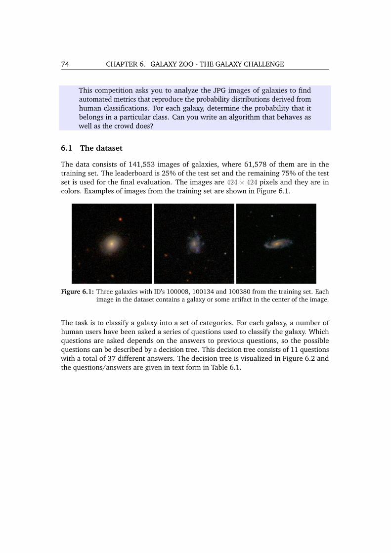
74 CHAPTER 6. GALAXY ZOO - THE GALAXY CHALLENGE
This competition asks you to analyze the JPG images of galaxies to findautomated metrics that reproduce the probability distributions derived fromhuman classifications. For each galaxy, determine the probability that itbelongs in a particular class. Can you write an algorithm that behaves aswell as the crowd does?
6.1 The dataset
The data consists of 141,553 images of galaxies, where 61,578 of them are in thetraining set. The leaderboard is 25% of the test set and the remaining 75% of the testset is used for the final evaluation. The images are 424 × 424 pixels and they are incolors. Examples of images from the training set are shown in Figure 6.1.
Figure 6.1: Three galaxies with ID’s 100008, 100134 and 100380 from the training set. Eachimage in the dataset contains a galaxy or some artifact in the center of the image.
The task is to classify a galaxy into a set of categories. For each galaxy, a number ofhuman users have been asked a series of questions used to classify the galaxy. Whichquestions are asked depends on the answers to previous questions, so the possiblequestions can be described by a decision tree. This decision tree consists of 11 questionswith a total of 37 different answers. The decision tree is visualized in Figure 6.2 andthe questions/answers are given in text form in Table 6.1.

CONCEPTS IN PREDICTIVE MACHINE LEARNING 75
Figure 6.2: The decision tree the users are taken through when classifying a galaxy on Galaxy-Zoo. This figure is taken from [Willett et al., 2013].
The task of classifying galaxies is not easy, and often the human classifiers disagree onthe questions in the decision tree. To quantify these disagreements, we are given dataon how the users distribute on the possible answers. The task is to predict how theusers of Galaxy Zoo distribute on the possible answers to each question. Say that for aspecific galaxy, 20% answers that the galaxy is “smooth”, 60% answers it is “features ordisk” and the last 20% answers that it is “star or artifact”, then the first three values inthe output for that galaxy will be
[0.2, 0.6, 0.2].
To put priority on the most important questions in the decision tree which determinesthe overall structure of the galaxy (the questions in the top of the tree), the laterquestions are down-weighted. Continuing the example above, look at the 60% whoanswered “features or disk”. These 60% now go to Question 2, and say that 70%answers “yes” and 30% answers “no”. Then the next two outputs for this galaxy will be
[0.6× 0.7, 0.6× 0.3] = [0.42, 0.18],

76 CHAPTER 6. GALAXY ZOO - THE GALAXY CHALLENGE
Task Question Responses Next01 Is the galaxy simply smooth and
rounded, with no sign of a disk?smoothfeatures or diskstar or artifact
0702
end02 Could this be a disk viewed
edge-on?yesno
0903
03 Is there a sign of a bar fea-ture through the centre of thegalaxy?
yesno
0404
04 Is there any sign of a spiral armpattern?
yesno
1005
05 How prominent is the centralbulge, compared with the restof the galaxy?
no bulgejust noticeableobviousdominant
06060606
06 Is the anything odd? yesno
08end
07 How rounded is it? completely roundin betweencigar-shaped
060606
08 Is the odd feature a ring, or isthe galaxy disturbed or irregu-lar?
ringlens or arcdisturbedirregularothermergerdust lane
endendendendendendend
09 Does the galaxy have a bulge atits centre? If so, what shape?
roundedboxyno bulge
060606
10 How tightly wound do the spi-ral arms appear?
tightmediumloose
111111
11 How many spiral arms arethere?
1234more than fourcan’t tell
050505050505
Table 6.1: The 11 questions and corresponding 37 different possible answers for the GalaxyZoo decision tree that users are taken through when classifying a galaxy.

CONCEPTS IN PREDICTIVE MACHINE LEARNING 77
since we distribute the 60% answering “features or disk” on the first question into twoparts of relative size 70% and 30%. Additionally, the answers to Question 6 have beennormalized to sum to 1.
6.1.1 Challenges with the data and interesting observations
Colors
An initial challenge with the data is the color in the images. Each image is representedby a 424× 424× 3 tensor, where the third dimension represents the colors red, greenand blue. This means that each image consists of 539,328 features. The three color-channels have a lot of information in common, and it is not clear whether the colorcontains any information, or whether converting the image to grayscale will preservethe information in the image.
Extracting image features
If we ignore the color aspect, each image sample still consists of 179,776 features. Withthis many features – many of which are highly correlated since pixels close to eachother are highly dependent – the most important aspect is to construct a new set ofgood features.
6.2 Evaluation metric
The scoring method in this competition is Root Mean Squared Error defined as:
RMSE =
√√√√ 1
37N
N∑i=1
37∑j=1
(tij − pij)2,
where tij is the actual value for sample i, feature j and where pij is the predicted valuefor sample i, feature j.
6.3 Approach and progress
The content in this subsection is written chronologically to give an understanding ofthe decisions and insights we got while trying to solve this problem. When mentioninga submission to the leaderboard which achieves a best score so far, we will mark thisscore with bold.
We started out by making a simple benchmark submission. For each of the 37 outputs,we computed the average value in the training data, obtaining a vector of 37 elements.Submitting this vector as the prediction for each image in the test set gave a RMSEscore of 0.16503.

78 CHAPTER 6. GALAXY ZOO - THE GALAXY CHALLENGE
To make it easier to extract features and learn from the image data, we pre-processedthe raw input images. The code for pre-processing is written in Python, using thescikit-image library. The pre-processing consisted of the following steps:
1. Threshold the image to black and white using Otsu’s method – which is a methodfor automatically inferring the optimal thresholding level.
2. Use a morphological closing operation with a square of size 3× 3 as kernel.
3. Remove all objects connected to the image border.
4. Remove all connected components for which the bounding box is less than 256 inarea.
5. Find the connected component C closest to the center of the image.
6. Rescale the bounding box of C to be a square by expanding either the width orthe height and add 15 pixels on each side.
7. In the original image, take out the portion contained in the expanded version ofC.
8. Rescale the image to 64× 64 pixels.
By performing the above steps, the images shown in Figure 6.1 are transformed to theimages shown in Figure 6.3.
Figure 6.3: The images shown in Figure 6.1 after pre-processing. The original images were424× 424 pixels, where the processed images are 64× 64 pixels.
Next we trained a convolutional neural network on the training data using the MATLABimplementation by [Palm, 2012]. The first layer in the network was a convolutionallayer with 6 output maps and a kernel size of 21. The second layer was an averagepooling layer with a scaling factor of 2. The third layer was a convolutional layer with12 output maps and a kernel size of 5. The fourth layer was an average pooling layerwith a scaling factor of 2. The final layer was a fully-connected layer with 37 outputneurons. All layers used the sigmoid activation function. To avoid overfitting, we

CONCEPTS IN PREDICTIVE MACHINE LEARNING 79
trained the network with a validation set of 5,000 images. If the error on the validationdoes not lower over 5 epochs in a row, we stopped the training and saved the networkwith the minimum validation error.
Training this network architecture on 10,000 of the 61,578 training images, we obtaineda leaderboard score of 0.13172. Training the same architecture on 30,000 images fromthe training data, we obtained a leaderboard score of 0.12056.
One way to get more performance out of a deep neural network, is to generate moretraining data using invariances in the data. One example of such an invariance in thegalaxy data is rotational invariance since a galaxy can appear in an arbitrary rotation.Other possible invariances are translation and scale, but since the galaxies after pre-processing do not have much space on either side (they tend to fill out the image),this is not as easy to exploit. We trained the same network as before on 55,000 ofthe training images (this is Network 2 in Appendix B), where each image was alsoadded after a rotation of 90 degrees, giving a total number of 110,000 training samples.Training the network took 80 epochs and a total of 53 hours.
When doing predictions on the test set, we sent each test image through the networkfour times, rotated 0, 90, 180 and 270 degrees, averaging the outputs. The validationerror on the network was 0.1113. Feeding 4 different rotations through the networkand averaging them gave a validation score of 0.1082. Finally, post-processing theoutput to obey the constraints of the decision tree reduced the validation error to0.1077. On the leaderboard this gave a score of 0.10884.
We extended the MATLAB library by [Palm, 2012] to have an additional fully-connectedlayer in the end of the network. Training with this extra layer did not improve theresults of the network.
Next we tried a different architecture for the network (this is Network 8 in Appendix B):
1. Convolutional layer with 6 output maps and kernels of size 5× 5
2. Factor 2 average pooling
3. Convolutional layer with 12 output maps and kernels of size 5× 5
4. Factor 2 average pooling
5. Convolutional layer with 24 output maps and kernels of size 4× 4
6. Factor 2 average pooling
7. Fully connected layer
This network reached a validation error of 0.1065 after 49 epochs (around 60 hours oftraining time). By inputting the test set with four different rotations and post-processing

80 CHAPTER 6. GALAXY ZOO - THE GALAXY CHALLENGE
the output, this gave a leaderboard score of 0.10449.
We then tried the following architecture (this is Network 10 in Appendix B):
1. Convolutional layer with 8 output maps and kernels of size 9× 9
2. Factor 2 average pooling
3. Convolutional layer with 16 output maps and kernels of size 5× 5
4. Factor 2 average pooling
5. Convolutional layer with 32 output maps and kernels of size 5× 5
6. Factor 2 average pooling
7. Convolutional layer with 64 output maps and kernels of size 4× 4
8. Fully connected layer
This network reached a validation error of 0.0980 after 76 epochs (around 160 hours).On the leaderboard this network obtained a score of 0.09655 (with post-processingand rotated test images).
6.3.1 Visualizations of the trained networks
Where normal neural networks are fairly hard to interpret, it is easier with convolutionalneural networks to understand what is happening. To understand how images areprocessed by the networks we have plotted some of the learnt kernels and visualizationsof how an image is propagated through the network.
For these examples we have used Network 10 (see Appendix B for a descriptionand comparison of the different networks trained) obtaining a leaderboard score of0.09655. In Figures 6.4 and 6.5 we have plotted the 8 and 16 kernels from the first twoconvolutional layers (in the third and fourth convolutional layer the kernels are toosmall to interpret). By visual inspection it is not completely intuitive what convolutionby these kernels is achieving.

CONCEPTS IN PREDICTIVE MACHINE LEARNING 81
Figure 6.4: The 8 learnt kernels in the first convolutional layer of Network 10.
Figure 6.5: The 16 learnt kernels in the second convolutional layer of Network 10. Note thateach of these 16 kernels is 3-dimensional and consequently each column of thisfigure corresponds to one kernel.

82 CHAPTER 6. GALAXY ZOO - THE GALAXY CHALLENGE
To get a better understanding of how the learnt kernels process the images we havetaken two different galaxies and propagated them through the network, this is seen inFigures 6.6 and 6.7. On the top is the original image which is input into the network.In the next layer the first 8 kernels have been applied, in the next layer the next 16kernels and so forth. Looking at the resulting output images after the first convolutiongives a better idea of what the kernels are doing. Some of the kernels are extracting avery rough outline of the galaxy (kernel 2 and 3 in Figure 6.6). Some of the kernelsare detecting the center of the galaxy (kernel 4 and 5 in Figure 6.6). Finally some ofthe kernels are detecting shapes/edges of some kind and consequently enhancing theshape of the galaxy (kernel 1,6,7 and 8 in Figure 6.6).
In the later layers of convolutions, the images are further broken down into differentlyshaped parts, extracting a reduced representation of the shape of the galaxy.
Figure 6.6: A visualization of how an image is propagated through the network. On the topis the original image which is input into the network. In the next layer the first 8kernels have been applied, in the next layer the next 16 kernels and so forth.

CONCEPTS IN PREDICTIVE MACHINE LEARNING 83
Figure 6.7: A visualization of how an image is propagated through the network. On the topis the original image which is input into the network. In the next layer the first 8kernels have been applied, in the next layer the next 16 kernels and so forth.
To get a better understading of the weaknesses of our networks we have determinedthe 9 galaxies in the validation set which gives rise to the largest errors. These galaxiesare shown in Figure 6.8. For some of them (the top left, the right in the center row, thebottom left and the middle one in the bottom row) it is easy to see what the issues are –either no galaxy is present in the image or multiple galaxies are present. For the twoimages where there is no galaxy present in the image the original images had largeartifacts and noise.

84 CHAPTER 6. GALAXY ZOO - THE GALAXY CHALLENGE
Figure 6.8: The 9 galaxies in the validation set which gives rise to the largest root mean squarederror. For some of these images it is very clear why the network is struggling.
6.4 Results and discussion
Since the Galaxy Zoo competition is not over until the 4th of April 2014, this sectionis written without knowledge of the winning submission and without knowledge ofthe final standings on the leaderboard. When this thesis was handed in, our latestsubmission held a 15th position out of 223 possible.

CONCEPTS IN PREDICTIVE MACHINE LEARNING 85
6.4.1 Choice of model
Convolutional neural networks are complicated when it comes to model complexity. Ifwe were to follow the hypothesis that simple models can get good results, starting outwith convolutional nets would not be a wise decision. There are multiple reasons forgoing directly to convolutional nets: The first reason is that we have a very large dataset(more than 50,000 data samples). The second reason is that the data has obviousinvariances (translation and rotation) which we can use to generate even more data.Finally, most recent litterature on image recognition points to convolutional nets as thebest possible approach [Ciresan et al., 2012]. One possible alternative approach wouldbe to use k nearest neighbors which would be very fast to implement. Unfortunatelythis approach (although simple) scales with the size of the dataset and consequentlybecomes relatively time-consuming.
Even though we do not know the inner workings of the other participants in the top ofthe leaderboard, we can still infer a bit of information from the forums and likewise.The person on the top of the leaderboard at this point, is Maxim Milakov, the author ofnnForge – one of the best implementations of convolutional neural networks available– who has specialized in using convolutional neural networks for his submissions.Multiple threads on the Kaggle-forum have also indicated that deep neural networks isthe solution participants are going for.
6.4.2 Speed of implementation
One significant issue was the speed of our implementation. When training the finalconvolutional nets the training time approached three weeks per network. In principlethere was no limit to amount of data we could generate, and there were multipleways to make the networks more complex. When training very complex models likeconvolutional neural networks, the efficiency of the implementation can be the decidingfactor. There are other implementations of convolutional neural networks written inC++ which also uses the GPU for computations, this leading to large speed-ups.
6.4.3 Predicting the right thing
The main short-coming of our current approach is that we are not predicting exactlythe correct thing. Regarding the error-measure we are doing the correct thing byoptimizing mean squared error for the net, but when we are training the network weare treating the problem as a regression problem instead of the multi-class classificationproblem it really is. The problem with this is that the output is actually limited by 11constraints which the networks are not utilizing (the answer-proportions for the 11different questions in the decision tree must sum to specific values).
A better way to handle this problem is to construct a network for multi-class classifica-tion using a number of so-called softmax units, and to derive a correct loss-function forthe network which incorporates the constraints of the decision tree directly.

86 CHAPTER 6. GALAXY ZOO - THE GALAXY CHALLENGE
Possible approach to modelling the correct loss function
The softmax function is a generalization of the logistic function which maps a vector ofk elements to a new vector of k elements:
σ(x)j =exj∑ki=1 e
xi.
The elements of the vector σ(x) are all between zero and one and they sum to one. Thesoftmax function is often used as the last layer in a neural network for classificationsince the outputted values will resemble probabilities.
For our special classification task, we can model the 11 different questions using 11distinct softmax units in the last layer. Now we can write the complete loss function inthe following way (using mean squared error instead of root mean squared error forsimplicity):
E = (t1a − p1a)2 + (t1b − p1b)
2 + (t1c − p1c)2 + (t2a − p2ap1b)
2 + . . . ,
where p1a is our estimate of the proportion of users choosing answer a to question 1and t1a is the actual proportion. Note that we now have that for each question, theanswer-proportions sum to 1 (as expected for a multi-class classification problem). Thereason for multiplying p2a and p1b is that users only see question 2 if they answer b toquestion 1. We wrote a Python-script to generate the complete loss function, whichtakes up more than 60,000 characters if written in the following format:
(T1a - P1a)ˆ2 + (T1b - P1b)ˆ2 + (T1c - P1c)ˆ2 + (T2a - P2a*P1b)ˆ2 +(T2b - P2b*P1b)ˆ2 + (T3a - P3a*P2b*P1b)ˆ2 + (T3b - P3b*P2b*P1b)ˆ2 +(T4a - P4a*P3a*P2b*P1b - P4a*P3b*P2b*P1b)ˆ2 +(T4b - P4b*P3a*P2b*P1b - P4b*P3b*P2b*P1b)ˆ2 + ...
To avoid implementing this loss function directly, an alternative approach is to transformthe target variables in an appropriate way. By using the description of the decision tree,we can transform the target values such that they sum to 1 for each of the 11 questions(thus making the “cumulative” probabilities into actual probabilities).
To motivate this idea, consider the following loss function:
E = (p1a − t1a)2 + (p1b − t1b)2 + (p1c − t1c)2 + (t1bp2a − t2a)2 + (t1bp2b − t2b)2 + . . . ,
which can be rewritten to the form:
E = (p1a− t1a)2 + (p1b− t1b)2 + (p1c− t1c)2 + t21b
(p2a −
t2at1b
)2
+ t21b
(p2b −
t2bt1b
)2
+ . . .
Here the fractions corresponds to new transformed target values, where we haverescaled the target variables such that the targets for each question will sum to one.

CONCEPTS IN PREDICTIVE MACHINE LEARNING 87
It is now possible to derive new gradients (and consequently δ’s) for this new errorfunction (where we have 11 softmax activation functions instead of the usual sigmoidactivation functions in the last layer).
Unfortunately, due to time-constraints we did not have time to implement this in theconvolutional neural network library.


Chapter 7
Conclusion
In this thesis we investigated competitive predictive machine learning, with a mainfocus on the platform provided by Kaggle. In Chapter 2 we stated a set of hypothesesabout the approaches to be taken in such competitions, namely that:
1. Feature engineering is the most important part.
2. Simple models can take you very far.
3. Ensembling is a winning strategy.
4. Overfitting to the leaderboard is an issue.
5. Predicting the right thing is important.
We investigated these hypotheses using information about the winning entries in pre-vious Kaggle competitions, by interviewing top participants from Kaggle and wherepossible by mathematical justification. Due to the diversity in the competitions at Kagglecombined with the breadth of data analysis approaches, nothing can be stated withabsolute certainty about predictive modelling. Still the five rather general hypothesesseem to be supported by our investigations.
As an attempt to describe more applicable methodologies for predictive modelling, weoutlined a conceptual framework in Chapter 3. This framework describes the processfrom data exploration, over data pre-processing to model training and finally selectingthe right model. We describe common tricks and techniques for different types ofproblems and provide some insight into the minds of the best predictive modellersthrough qualitative interviews. Since no two datasets are the same, and since thefield of machine learning is under constant development, it is not possible to state aperfect recipe for winning a competition at Kaggle. Still by utilizing the lessons learntby previous competitors one can without too much previous experience obtain decentresults.
89

90 CHAPTER 7. CONCLUSION
To get a better understanding of the mechanics of Kaggle, to validate our hypothesesand to test out the conceptual framework we participated in two competitions at Kaggle.In the challenge posed by Expedia – described in Chapter 5 – the task was to rank hotelsby their likelihood to be booked. In this competition we obtained a not very impressiveranking of 138th place out of 337 possible. Looking at the description of the winningsolutions our approach was doing most of the things correctly, but a few importantthings were overlooked. Firstly we might have handled missing values in the wrongway by simply imputing the median value for many features. Secondly our methodsdid not take the order/position of the hotels into account which had a very clear effect.Finally one could reduce the training data dramatically with under-sampling whileactually gaining better results. Most likely, these errors combined is the reason weended up in 138th place – but it is also possible that some part of the result can beattributed to erroneous implementations by us.
In the challenge posed by Galaxy Zoo – described in Chapter 6 – the task was toclassify galaxies by their shape given image data from deep space telescopes. Since thiscompetition is not over yet, it is not possible to conclude completely on the results. Stillwe can say that our solution using deep neural networks is doing a fair job (at this timeranked 15 out of 223 on the leaderboard).
There is no doubt that competitive machine learning will be an important trend bothin the academic community and for businesses in the future. Kaggle has provideda platform for running these competitions and so far the results obtained using theplatform look very promising. Like for most other scientific challenges, no perfectalgorithm exists for creating a winning solution on Kaggle since these often requirecreativity, patience and a bit of luck. Nevertheless, the methods and rules of thumbprovided in this thesis can form a solid foundation for new participants in the future.

Appendix A
Previous Competitions
In this appendix we have summed up some details from 10 of the most recent com-petitions on Kaggle. We shortly describe the objective of the competitions and quotethe description of the solutions by the Top-3 participants. Throughout the thesis, thesecompetitions are referenced with the following abbreviated names: FACEBOOK, SUNNY-HASHTAGS, SEECLICKPREDICT, BIRD, ACCELEROMETER, SOLARENERGY, STUMBLEUPON,BELKIN, BIGDATA and CAUSEEFFECT.
A.1 Facebook Recruiting III - Keyword Extraction
A.1.1 Objective
This competition tests your text skills on a large dataset from the Stack Exchange sites.The task is to predict the tags (a.k.a. keywords, topics, summaries), given only thequestion text and its title. The training set is large, consisting of millions of questions.The evaluation metric was Mean F1-Score – meaning that the competitors shouldpredict a set of candidate tags, some which might not even be present in the trainingset.
A.1.2 Winning entries
1st: Owen
My approach:
1. Take duplicates out like many others did
2. Calculate the association between all 1-gram and 2-grams in title andbody. I kept the first 400 chars and last 100 of body to keep the size undercontrol. I keep only the top 30 tags for each 1-gram and 2-gram
3. Predict the tags by combining all the tags associated with all the 1-gram and 2-grams in Title+body. Each 1/2 gram’s impact is weighted by
91

92 APPENDIX A. PREVIOUS COMPETITIONS
its support and entropy. The entropy part only improve the score verymarginally.
4. Take the top tags based on their score. The cut off threshold is determinedby the ratio between the score of tag k and the average score of all tagswith higher scores than k.
5. I scored the above on 200k posts in training, and computed the bias foreach predicted tag. Some tags have more FP than FN, some have more FNthan FP. The goal is to have FP and FN about equal.
6. Score test data and adjust for the tag bias from step 5, i.e., if a tag has#FP > #FN , decrease its score, and vice versa.
Note: There are quite a number of tuning parameters that I “hand optimized”by evaluating the impact on 2% of training data I kept as a validation dataset.Title is much more important than body – I gave a 3:1 weight to title (butthis is somewhat cancelled out by the fact that there are more words inbody usually) I thought about doing some extraction but didn’t get time todo so. I also extracted quoted posts in the body and tried to match that withtraining, just like the duplicates. But this barely improves the result. So itseems the association of tags between posts and quoted posts are not verystrong. I also tried some TF-IDF based methods but didn’t get good results.I didn’t spend too much time on “NLP” like tasks such as stemming/tagging,etc. Part of the reason is time required, and part of reason is that the postsare not very “natural”, compared to texts from news archives and books.I figure I probably would lose as much information on the code part, v.s.what I can gain in the “natural language” part.
The “RIG”: As noted by everyone, the bottleneck of this competition is RAM.I am fortunate enough to have access to a machine with 256GB ram to tryout different parameters.
The final solution would run on a desktop with 64GB of ram in about 4hours. The training only takes about 1.5 hour and scoring will take 2.5– partially because it runs out of ram. Training of the model will eat upalmost all of the 64GB, and the rest will swap to disk. There has to be atleast 90GB swap space for this to run with out error.
I used Python, which is not very “memory efficient”. If we were to competeon “efficiency” I think c/c++ would be necessary.
2nd: Ruslan Mavlytov
This solution was not described anywhere.
3rd: E. G. Ortiz-Garcıa
This solution was not described anywhere.

CONCEPTS IN PREDICTIVE MACHINE LEARNING 93
A.2 Partly Sunny with a Chance of Hashtags
A.2.1 Objective
In this competition you are provided a set of tweets related to the weather. Thechallenge is to analyze the tweet and determine whether it has a positive, negative, orneutral sentiment, whether the weather occurred in the past, present, or future, andwhat sort of weather the tweet references.
A.2.2 Winning entries
1st: aseveryn
As a core prediction model I used Ridge regression model (of course withCV to tune up alpha). I saw most of the people ended up using Ridge aswell. I tried SGD and SVR but it was always worse than simple Ridge. Myset of features included the basic tfidf of 1,2,3-grams and 3,5,6,7 ngrams. Iused a CMU Ark Twitter dedicated tokenizer which is especially robust forprocessing tweets + it tags the words with part-of-speech tags which canbe useful to derive additional features. Additionally, my base feature setincluded features derived from sentiment dictionaries that map each wordto a positive/neutral/negative sentiment. I found this helped to predict Scategories by quite a bit. Finally, with Ridge model I found that doing anyfeature selection was only hurting the performance, so I ended up keepingall of the features ∼1.9 mil. The training time for a single model was stillreasonable.
Regarding the ML model, one core observation, which I guess preventedmany people from entering into the < .15 zone, is that the problem here ismulti-output. While the Ridge does handle the multi-output case it actuallytreats each variable independently. You could easily verify this by trainingan individual model for each of the variables and compare the results. Youwould see the same performance. So, the core idea is how to go abouttaking into account the correlations between the output variables. Theapproach I took was simple stacking, where you feed the output of a firstlevel model and use it as features to the 2nd level model (of course you doit in a CV fashion).
In my case, the first level predictor was plain Ridge. As a 2nd level I usedEnsemble of Forests, which works great if you feed it with a small numberof features – in this case only 24 output variables from the upstream Ridgemodel. Additionally, I plugged the geolacation features – binarized valuesof the state + their X,Y coordinates. Finally, I plugged the outputs from theTreeRegressor into the Ridge and re-learned. This simple approach gives anice way to account for correlations between the outputs, which is essentialto improve the model.

94 APPENDIX A. PREVIOUS COMPETITIONS
Finally, a simple must-not-to-forget step is to postprocess your results – clipto [0,1] range and do L1 normalization on S and W, s.t. the predictionssum to 1.
2nd: Tim Dettmers
I used deep neural networks with two hidden layers and rectified linear units.I trained them with stochastic gradient descent and Nesterov’s acceleratedgradient on GPUs and used dropout as regularization with which I couldtrain a net in 30 minutes. One thing which I have not seen before but greatlyimproved my results was to use what is best denoted as “dropout decay”,i.e. reducing dropout together with momentum at the end of training alongwith a linear decreasing learning rate - this seemed to keep hidden activitiesdecoupled while at the same time introduced more information into thenetwork which was quickly utilized and decreased the cross validation errorby quite a bit.
I tried unsupervised pretraining with both restricted Boltzmann machinesand several types of autoencoders, but I just could not get it working and Iwould be interested to hear from anyone for whom it worked.
Random sparse Gaussian weight initialization was much faster to train thanrandom uniform square root initialization - and it might have also increasedgeneralization, but I did not test this thoroughly.
Other than that I also used ridged regression and random forests regression.The later model performed rather poorly but made errors which were verydifferent from my net and thus decreased the error in my ensemble.
I split my cross validation set into two and fitted least squares on one halfto get the best ensemble.
3rd: Duffman & Pascal
At first a quick tfidf with RidgeRegressor and clipping to 0, 1 lower andupper bounds got me .152, but I found out after playing with the parametersthat it was easy to fall into local optima since the columns each behavedwildly different. When I joined up with Pascal, we decided to try and doa more customized approach since trying to find a global optima for allcolumns just wasn’t realistic.
Base Models: A quick summary is that we created models based on thecombinations of char/word, tfidf/countvec, Ridge/SGDregressor/Linear-Regression, and S, W, K Block. So that’s 2 * 2 * 3 * 3 for 36 models. Themodels parameters were optimized based on some custom code (writtenby the amazing Pascal!) to find the best parameters so we don’t have tooptimize 36 models individually. We cut out 12 models worth of featuresby simply putting it on a spreadsheet and doing some analyses to see if it

CONCEPTS IN PREDICTIVE MACHINE LEARNING 95
adds any variance or not. We probably could have used Recursive FeatureSelection and we did eventually, but the RFE took a ridiculously long timefor us to test so we decided to use a spreadsheet to get an idea of howmuch we should remove before we actually used it. The vast majority ofour submissions was just playing around with the various models and howthey fit into our final ensemble.
Ensemble: We did a stack with RidgeRegression at the end. The reasonwe did a stack rather than a weighted averaged blend was we wantedto have the other columns help predict each other. So K columns wouldhelp predict w columns and vice versa. It also allowed for optimization bycolumn automatically rather than optimizing by all columns that might notbe relevant to each other.
We also tried ExtraTreesRegressor ensemble and that gave us an amazingboost to our CV, but not to the LB which was a first. In our case, we madethe right choice not to trust the CV since I was sure there were train/testset differences causing it.
For a final boost, we did several more stacks with different splits since thefinal stack was determined by 70/30 split and blended them. That way wecan come close to using all the trianing data for the stack.
A.3 See Click Predict Fix
A.3.1 Objective
The purpose of this competitions is to quantify and predict how people will react to aspecific 311 issue. What makes an issue urgent? What do citizens really care about?How much does location matter? The dataset for the competitions contains severalhundred thousand 311 issues from four cities. Your model should predict, for eachissue in the test set, the number of views, votes, and comments.
A.3.2 Winning entries
1st: J.A. Guerrero
My first submissions were based in naive dataset with features like:
- day(from 0 to 625)
- latitude
- longitude
- hour (beginning at 6:00 am)
- week day (beginning on Monday)
- summary len
- description len

96 APPENDIX A. PREVIOUS COMPETITIONS
- city (factor)
- tag type(onehot of categories with more than 20 cases)
- source(onehot of categories with more than 20 cases)
With this data and using R gbm I get results in 0.304x training the last 60days. More training days always fit worst, and I realized optimizing thenumber of trees for different periods of training reflected in very differentnumber of trees for reasonable values of learning rates. So for gain robust-ness I decided use small learning rates in all the models, 0.002 to 0.0005for guarantee a more stable error curve.
Using absolute time feature (day) in a time series model has an obvious risk.You easily can learn time anomalies in training period but the extrapolationto the test period could be a lottery. Linear models project the data ina linear trend. Tree based models will assume the test period is like thelast days of training period: always day feature is used in a subtree, theday values presents in test period are in the same branch that last trainingperiod.
In this case we were lucky so the test period means value were like the endof training period, but this could be different in a future. This fact leadsme to open a new question: Was RMSE the best metric for this dataset?I personally think not, I see more interesting a ranking of issues than anexact estimation of number of votes and this would have prevented againstcalibration issues we’ve seen in this competition. In my definitive analysisI’ll use Spearman rank coefficient too for model benchmarking.
But the metric was RMSE so my objective was build features time indepen-dents and use the full period of training.
The hypothesis were:
- The response to an issue depends (directly or inversely) of number ofrecent issues and similar issues (time dimension).
- The response to an issue depends (directly or inversely) of number ofissues and similar issues reported close (geographic dimension).
- There are geographic zones more sensitive to some issues (geographicdimension).
With that in mind I defined three time windows, (short, middle and long)of 3, 14 and 60 days and three epsilon parameters (0.1, 0.4 and 1.2) foruse them in a radial basis distance weighted average for each issue. Theselection of this values were for adjust the decay shape in a way the weightsrepresent city, district and neighbour ambits.
The tag type were grouped in: crime n social, rain snow, traffic, lights,trees, trash, hydrant, graffiti, pothole, NA, Other.

CONCEPTS IN PREDICTIVE MACHINE LEARNING 97
For each issue (row) I computed 3 (short, middle, long) x 3 (city, districtand neighbour) features for each of 11 tag group. Each feature uses radialbasis weights respects the distance in kms between issues.
I computed 3 x 3 features for the total of issues and for the issues of thesame group, so in total I had 3 x 3 x 13 of such features, all computed witha LOO (Leave One Out) criteria for avoid overfitting. This 117 feature set Inamed LOO features.
For a period of last 150 days and for each issue I computed the LOOweighted radial basis average for comments, votes and views for (city,district and neighbour) params (9 features) and the same but filtered tothe issues in the same group (other 9 features). This 18 features I namedBAYES features.
LOO and BAYES featured were normalized to (0,1) range for use with linearmodels too.
For summary I computed a bag of more frequents words (> 50). NamedBOW.
I fitted several models: (gbm, RF, glm) for (basic data, basic + LOO, basic+ LOO + BAYES, basic + LOO + BAYES + BOW)
In the basic data added to other features I didn’t used “day” feature forcingthe model to learn the time anomalies from LOO features. I used longitude& latitude, but really the model learned from LOO very well too: longitudeand latitude weren’t neccesary.
Some models I fitted segmented by cities and almost all I used a “big column”approach for training the three responses all together. The models fittedwith “big column” were systematically better than trained each responsealone.
For the final blending I used the same method that James Petterson (BigChaosmethod of netflix prize) introducing some dummies models for each re-sponse and each city (all 0 except a city or a response).
Edit: And, of course, all done in log(x+1) scale and reversed to exp(x-1)
2nd: Bryan Gregory & Miroslaw Horbal
Overall I trusted CV for every decision I made for my model. My CV methodwas to chop off the final 20% of the training data (which worked out to be44626 issues)
I treated scaling and selecting the number of issues to use at training timeas a hyperparameter selection problem, so both my choices for scales andthe number of training examples was selected from cross validation. I alsoused segmented scaling similar to Bryan, but my segments were brokendown into:

98 APPENDIX A. PREVIOUS COMPETITIONS
Chicago, Chicago remote-api-created, Oakland, Oakland remote-api-created,New Haven, and Richmond
As Giovanni guessed, I focused a lot more on text-based features and TFIDFactually gave me the biggest single gain over any other features.
I trained a Ridge model on log(y + 1) targets and engineered the followingfeatures:
- TFIDF vectorization for summary and description up to trigrams
- boolean indicator for weekend
- log(# words in description + 1)
- city (one hot encoding)
- tag type (one hot encoding)
- source (one hot encoding)
- time of day split into 6 4h segments (one hot encoding)
Along with those base features I also generated higher order combinationsof some of the categorical features to produce new categorical one hotencoded features, these included:
- (city, time of day)
- (city, source)
- (city, tag type)
- (source, tag type)
Furthermore, I added 2 extra geographic features using data collected froma free geocoding service, these included:
- zipcode
- neighborhood name
and the combination:
- (zipcode, source)
Since there were a lot of sparse elements in my dataset I threshold anyrare categories using various techniques. For tag type, and higher ordercombinations I replaced any rare categories with a single “ rare ” category.For zipcode and neighborhoods I used a knn clustering heuristic I hackedtogether that essentially grouped rare zipcodes/neighborhoods with theirnearest euclidean neighbour (lat, long) using an iterative process
Also, Bryan noticed that votes never drop below 1, so I was able to squeezeout a few extra points by setting 1 as a lower bound on votes.
Overall this model would score around 0.29528 on the private leaderboard.I think the main reason why Bryan’s model and my model blended sowell was primarily due to us independently coming up with very different,

CONCEPTS IN PREDICTIVE MACHINE LEARNING 99
equally powerful models that each had their own strengths. We gained0.0035 on our score by applying a simple 50/50 weighted average as Bryandescribed.
3rd: James Petterson
This solution was not described on the forum.
A.4 Multi-label Bird Species Classification - NIPS 2013
A.4.1 Objective
The Neural Information Processing Scaled for Bioacoustics (NIPS4B) bird song competi-tion asks participants to identify which of 87 sound classes of birds and their ecosystemare present in 1000 continuous wild recordings from different places in Provence,France. The training set contains 687 files. Each species is represented by nearly 10training files (within various context / other species).
A.4.2 Winning entries
1st: Mario
Given in an external paper [Lasseck, 2013].
2nd: les bricoleurs
you can make a ∼0.895 model by
- split each clip into half-second windows overlapping by 80%. for eachwindow, determine the average value of each mfcc coefficient. (so you have16 features for each window)
- use a random forest classifier with 87 yes/no outputs
- average the probabilities for each window to get the probability for theentire clip
A longer description is available on the forum of the competition.
3rd: Rafael
Now as regards my approach it is an RF in a multilabel setting (so calledBinary Relevance). That’s all.
selector = RandomForestClassifier(n estimators=80, random state=SEED)
selector.fit(train x, train y)
xTrain = selector.transform(train x)
xTest = selector.transform(test x)

100 APPENDIX A. PREVIOUS COMPETITIONS
model = RandomForestClassifier(n estimators=250, criterion=’entropy’,max depth=None, min samples split=4, min samples leaf=3, max features=’auto’,bootstrap=True,oob score=True, n jobs=1,random state=SEED, verbose=0)
classif = OneVsRestClassifier(model)
classif.fit(xTrain, train y)
preds = classif.predict proba(xTest)
train y is the given 687x88 binary matrix of species ( I include noise classand then remove it during submission).
train x is column stacked features matrix from 3 different sources.
Source 1: Treat spectrogram as picture, extract ROI’s, superimpose ROI’s onthe initial spectrogram and keep only the enhanced spectrum (see attachedfigs). Partition the picture in 16 equal horizontal bands and derive mean,std, median, kurtosis and 90% percentile. Tried several others (entropy,skewness etc). Did not work. So first features 5x16 = 80 per recordinga 687x16 training matrix). Only with these you get about 86.5 on bothleaderboards. Code to extract ROI’s is available both in matlab and python.
Source 2: Make a bag of measurements for each recording by measuringproperties of each ROI. Everything I could find in ndimage angle BW andduration of each ROI. These measurements are coded using 3 Kmeans of75, 25 and 15 centres (resulting to 100 features per recording. So S2 is687x100. HOGs did not work for me and the gain was only getting to afinal about 88%.
Source3: The most powerful feature is the one introduced by Belunga inMLSP bird challenge continuing on Nick Kridler’s approach on whales. It isbased on deriving normalized cross-correlation of ROI’s with the spectrum.This leads to a 687x33000 matrix. I did a variation here: I keep ROI’s oftrain and test into sorted lists (frequency the key) and I calculate cross-correlation only if a ROI of training set fits a ROI of test set in terms offrequency range and duration. This leads to most correlations to be setto 0 without being calculated. This way the matrix is calculated very fast.Belunga’s is a bit more accurate I admit but takes too much time for thiscompetition (many days on an I7 16GB RAM).
Averaging over 10 models with different seeds unexpectedly gave a boostfrom 90.6 to 91.6 in the public ldb. The rest was by putting the last 15lower probs per recording to a v.small costant.
A.5 Accelerometer Biometric Competition
A.5.1 Objective
Given is approximately 60 million unique samples of accelerometer data collected from387 different devices. These are split into equal sets for training and test. Samples in

CONCEPTS IN PREDICTIVE MACHINE LEARNING 101
the training set are labeled with the unique device from which the data was collected.The test set is demarcated into 90k sequences of consecutive samples from one device.A file of test questions is provided in which you are asked to determine whether theaccelerometer data came from the proposed device.
A.5.2 Winning entries
1st: gaddawin
Well, my approach was similar to others:
1) find consecutive sequences and build chains. I used logistic regres-sion over some simple features (time interval between sequences (only<1000ms), coords difference, etc) to find consecutive sequences. I spentmuch time trying to make chains longer and longer. But there are no se-quences with duration >1 hour (it seems that they were deleted duringdata preparation). So, it is impossible to build very long chains.
2)It’s easy to predict true device for long chains (except chais with 2 devicesas Jose mentioned).
3)For sequences in “bad” chains i used random forest classifier with 5features (sampling rate difference, time of day, etc )
4)It is possible for many devices to find sequences (and chains!) that are“consecutive” (day was changed during data preparation, but time of dayremains the same) to last device record. Predicting device for these chainsis very easy.
2nd: Solorzano
As for methods, my top entry was a blend of 24 models. Some of them areconventional single-sequence models, both leak-based and non-leak-based.But the most accurate models (individually scoring up to 0.993) are basedon lists of sequences (which I call sequence chains) where only the frequencyof the professed device is considered, using a binomial distribution. A lotcould be said about the best ways to build probable sequence chains, but Iwon’t get into that.
In some cases, the professed device IDs that label sequences in a chain arenot informative. For example, a chain might have only 2 professed deviceIDs total. In such cases, it helps to apply conventional classifiers to theindividual sequences of the chain, and combine the results.
3rd: Target Leak Model
This solution was not described anywhere.

102 APPENDIX A. PREVIOUS COMPETITIONS
A.6 AMS 2013-2014 Solar Energy Prediction Contest
A.6.1 Objective
The goal of this contest is to discover which statistical and machine learning techniquesprovide the best short term predictions of solar energy production. Contestants willpredict the total daily incoming solar energy at 98 Oklahoma Mesonet sites, whichwill serve as “solar farms” for the contest. Input numerical weather prediction datafor the contest comes from the NOAA/ESRL Global Ensemble Forecast System (GEFS)Reforecast Version 2. Data include all 11 ensemble members and the forecast timesteps12, 15, 18, 21, and 24.
A.6.2 Winning entries
1st: Leustagos & Titericz
Our approach to this problem didnt used much feature engineering. Weused mostly raw features.
Guidelines:
We used 3 fold contiguous validation (folds with years 1994-1998, 1999-2003, 2004-2007)
Our models used all features of forecast files without applying any prepro-cessing, so we took all 75 forecasts as features
For each station, we used the 75 forecasts of 4 nearest mesos. So with thiswe had 75x4 such features.
Besides those forecast features we had the following: month of the year,distance to each used meso, latitude difference to each meso. In total it wasaproximately 320 features (with the forecast ones).
We trained 11 models for this, one for each forecast member (the 11independent forecasts given)
We averaged those 11 models optmising MAE.
We used pythons GradientBoostedRegressor fo this task.
Thats it!
2nd: Odeillo
I also used a similar approach:
- first averaged the 11 forecast members (as Owen)
- used the whole training set
- used the 75 features (15 x 5 hours)
- added Month + Elevation + Lat + Lon (nevertheless only Month gaveinteresting correlations)

CONCEPTS IN PREDICTIVE MACHINE LEARNING 103
- for each of the 98 mesonet I made a linear interpolation of the four nearestGEFS points (weighted by the distance). This was the step that reallyimproved my score!
- dswrf and pwat clearly appeared to be the most important and I addedderived features for them. For example dswrf(H3)- dswrf(H2)
- used gradient boosting techniques with a program written in C#
During the competition, the Admin added the elevations of the GEFS but Iwas unable to find any interesting correlations with them.
3rd: Owen
I used a similar approach:
* No feature engineering except for a linear combination of dswrf at the 5different time points.
* Averaged the 11 forecast members as the first step
* Kept all 75 features
* Used GBM in R, with “laplace” distribution to optimize for MAE
* Built 2 GBMs, one based on the 75 features from the nears mesos, onebased on the weighted average of the 75 features (inversely proportional todistance) of the nearest 4
* Similar to the winning team’s approach, also included days of year, andlong/lat in the model.
A.7 StumbleUpon Evergreen Classification Challenge
A.7.1 Objective
StumbleUpon is a user-curated web content discovery engine that recommends relevant,high quality pages and media to its users, based on their interests. While some pagesthey recommend, such as news articles or seasonal recipes, are only relevant for ashort period of time, others maintain a timeless quality and can be recommended tousers long after they are discovered. In other words, pages can either be classified as“ephemeral” or “evergreen”. The mission is to build a classifier which will evaluate alarge set of URLs and label them as either evergreen or ephemeral.
A.7.2 Winning entries
1st: fchollet
Features: raw Tf-idf + pca of the output of a tf-idf transform, for thefollowing:
- url

104 APPENDIX A. PREVIOUS COMPETITIONS
- text (body)
- titles + “keywords” metatags (why this combination? mainly becausesome pages lack metatags, and the closest thing are the titles)
- text + url + metatags for “keywords” and “description” + “alt” values forimg tags + possibly titles (which is pretty much the combination of all dataI extracted from the pages –I might have eliminated titles from the mix afterfinding they did not impact results much due to redundancy edit: actuallytitles were indeed included here) So, for all these sets of terms, compute ineach case a Tf-idf, then train a PCA on the output.
Then each resulting set of vectors will be classified with a Random Forest(PCA vectors) and a Logistic Regression (raw vectors). That’s 4*2 arrays ofpredictions, which are then merged with a simple linear classifier. I alsoexperimented with SGD and a few others, not sure if they were part of thecode that generated the winning submission, I’ll dig into it. edit: SGD wasnot used for the winning submission, only LR and RF
Anyway that’s it: “classical” classifiers (LR & RF) run on the tf-idf (or tf-idf +pca if necessary) of terms extracted from urls, texts (body), titles, metatags,and alt img tags –then predictions merged with a linear classifier. Eachclassifier was tuned separately (grid search).
One more thing: it might be interesting for the StumbleUpon engineers tonote that working *only* with the urls gets you 90% of the way there. Soyou can be extremely accurate without even having to fetch a page, andwith very little computation. In production I’d use something like this.
2nd: Maarten Bosma
First let me say: Variance was crazy in this composition. My third place(private score 0.88817) scored only 0.88027 on the public leader board. Ittook quite some nerve to select it as my final submission.
I actually made another submission, which would have won had I selectedit (Public: 0.88167, Private: 0.88915). I though the other result was morerobust, even though that one had a higher CV score and lower variance.You can really image me banging my head on the table right now. I think,the lesson here is: if you are paranoid enough about overfitting you cantrust your CV score.
My first key insight was: this competition is not about which pages arelong lasting. This is first and foremost about what people find interesting.The main topics of interest is food (especially recipes). Other topics arethat are mixed (but mostly evergreens) are health, lifestyle and excise.Seasonal recipes are actually mixed too. Supposedly funny videos/pics,technology, fashion, sports, sexy pictures are mostly ephemerals. Somesites are in languages other than English, these are mostly (but not all)

CONCEPTS IN PREDICTIVE MACHINE LEARNING 105
ephemerals. Sometimes the frontpage of a news site was in there (e.g.http://www.bbc.co.uk)→ ephemeral.
My second key insight was: the features other than text are useless. I onlyused text features.
I used an html parser and to actually parse the html that was given. I thengave different weights to each tag (h1, meta-keywords, title, ...). I alsoused the given boilerplate and a boilerplate that I extracted myself with atool called boilerpipe. I had more than 100 of these weighted sets. I thenused raw (normalized) counts, stemming, tfidf, svd and lda to preprocessthem. For each of those more than 300 sets I used logistic regression to getpredictions, which I than combined into an ensemble.
I did not use n-grams, but should have.
I also tried to use meta feature: how many words, what kind of words(pos-tag distribution, common/uncommon, ratio in dictionary) .... The ideawas that items with a good (easy to read) writing style are more likely to beevergreens. I got 0.83 out of these features alone, but they did not seem toadd anything to the ensemble.
I also have a little bit of secret sauce. Something that I spend quite sometime on. This eventually just added a little bit to the final ensemble, butmaybe is something I will explore more in future competitions.
3rd: michaelp
This solution was not described anywhere.
A.8 Belkin Energy Disaggregation Competition
A.8.1 Objective
In this competition, the participants are given a dataset of readings from the Elec-tromagnetic Interference (EMI) that most consumer electronic appliances produce toidentify signatures. Examples of such signatures can be seen in Figure A.1.

106 APPENDIX A. PREVIOUS COMPETITIONS
Figure A.1: Frequency spectrogram showing device actuation in a home. Taken from[Gupta et al., 2010].
A.8.2 Winning entries
1st: jessica bombaz
It was really a difficult task to detect the correct appliances. Althoughthere are various data sources available, sometimes I found it impossibleto distinguish or even detect low signal appliances due to high signal-to-noise ratio. This difficulty is also reflected in the final scores, as anyoneof us managed to predict only about 0.04 / 0.08 = 50% of all the givenappliances. I wonder, how much the score would be, if we took togetherthe correctly predicted appliances of all the participants?
Basically I used also the first time differences to detect peaks. Instead ofcomputing s(t+1) - s(t) which might be vulnerable to sampling frequencyand also increases noise, my algorithms compute the mean of two timewindows separated by some delay. Only then I took the difference. Forthose appliances with a characteristic signal, I computed the similarity byintegrating over the squared difference. This works surprisingly well even ifthe signal is noisy.
2nd: Luis
My approach is still similar to the edge detection and differences in thepower, but I will still describe it.

CONCEPTS IN PREDICTIVE MACHINE LEARNING 107
First at all, I did not use any information from the HF data. I did not evenlook at it. My plan was originally to extract as much information from thepower as I can and then go back to use the HF information. Later, I did nothave time to go back and explore the HF data.
For each of the appliances I have a window of 12 time ticks ( 2 seconds) thatcontain the “turning on” signature and another window for the “turningoff” signature. The first 3 time ticks contain the power when the applianceis still off, and the remaining contain the power when the appliance is on.The number 12 is not fixed. I use different numbers for some appliances.There is a trade off for that number. For large numbers, the system is morerobust to noise. For low numbers, the system is more capable of identifyingappliances that are turned on or off at the same time.
For a new test day, I have a window that runs through each time tick of theday and is compared to the “turning on” signatures of each appliance. Whenthe running window is very similar to one of the appliances signatures, thesystem mark that the appliance has been turned on. The same is doneindependently for the “turning off” signatures. Finally, I pair the “turningon” events with the “turning off” events. That is the basic algorithm.
My system is capable of identify appliances that are turned on very closein time (the difference in time should still be at least 1 second). However,it has limitations for low power appliances and it is unable to successfullydistinguish appliances that are very similar.
3rd: Titan
I also used time differences (first derivative) to detect occurrence of eventswhich as Rosnfeld already mentioned is critical. I used an edge detectionalgorithm for the power signatures to detect events and measure the sizeof the jump in each value from before and after the event happened. Asummary of the results is shown in our visualization entry.
I could see few transient HF signals that lasted more than a second andeven for those the one second resolution of the HF data was too coarse to beuseful because in some cases the transient was concentrated in one secondgiving a clear signal and in other cases it was split between two consecutiveseconds resulting in a weaker signal for each of the seconds that was hardto distinguish from the noise.
For each event, I averaged the HF data for several samples after the eventand subtracted the average from several samples before the event. I thenaveraged these HF difference over multiple events to get steady state HFsignatures for each appliance (plotted in the HFdiff figures of the visual-ization entry). In theory, these HF signatures should have allowed me todistinguish between appliances that had nearly identical power signaturesand the theory worked well in some cases.

108 APPENDIX A. PREVIOUS COMPETITIONS
These were some appliance pairs for which even the HF signatured I gener-ated were not clear enough to distinguish between them and other pairswhere the back-end solution did not seem to match what the HF signatureswere telling me. In some cases it was more effective to choose the laundryroom lights based on whether the Washer/Dryer were working at the sametime than to rely on the HF signatures.
A.9 The Big Data Combine Engineered by BattleFin
A.9.1 Objective
The first stage of the competition is a predictive modelling competition that requiresparticipants to develop a model that predicts stock price movements using sentimentdata provided by RavenPack. You are asked to predict the percentage change in afinancial instrument at a time 2 hours in the future. The data represents features ofvarious financial securities (198 in total) recorded at 5-minute intervals throughout atrading day. To discourage cheating, the features’ names or the specific dates are notprovided.
A.9.2 Winning entries
1st: BreakfastPirate
A high-level description of my approach is:
1. Group securities into groups according to price movement correlation.
2. For each security group, use I146 to build a “decision stump” (a 1-splitdecision tree with 2 leaf nodes).
3. For each leaf node, build a model of the form Prediction = m * LastObserved Value. For each leaf node, find m that minimizes MAE. Rows thatmost-improved or most-hurt MAE with respect to m=1.0 were not included.
2nd: SY
My model was designed with one main principle in mind: to make modelas simple as possible and as stable as possible to avoid overfitting. My finalsubmission was a weighted mean of three very similar models. Blending,however, generated very small gain in this particular case. That is why hereI will be describing single model that was a part of the blend. This modelby itself has 0.40959 score on public leaderboard and 0.42378 on private,which is enough to be # 5 on public and # 3 on private leaderboards.
An extremely long model description is not presented here, but can be found on theforums.
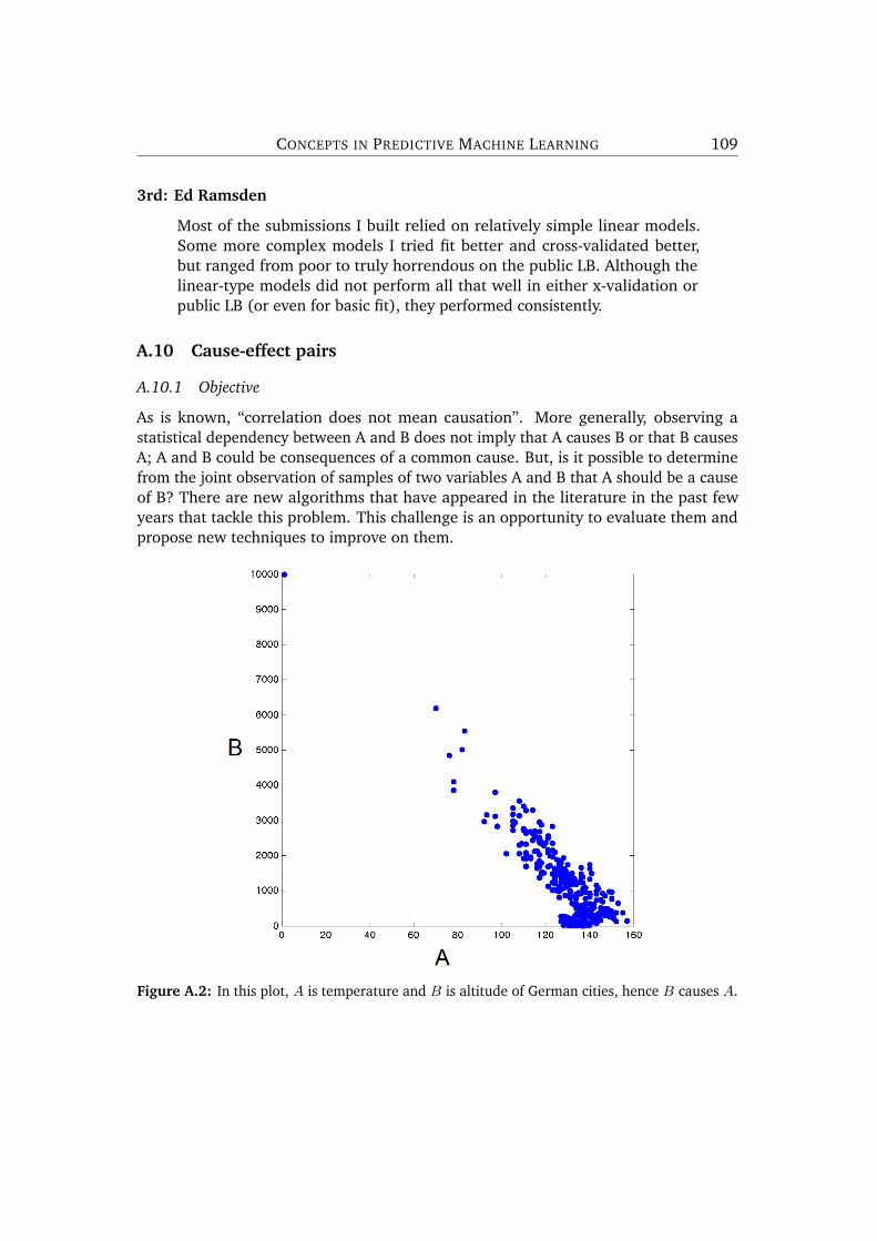
CONCEPTS IN PREDICTIVE MACHINE LEARNING 109
3rd: Ed Ramsden
Most of the submissions I built relied on relatively simple linear models.Some more complex models I tried fit better and cross-validated better,but ranged from poor to truly horrendous on the public LB. Although thelinear-type models did not perform all that well in either x-validation orpublic LB (or even for basic fit), they performed consistently.
A.10 Cause-effect pairs
A.10.1 Objective
As is known, “correlation does not mean causation”. More generally, observing astatistical dependency between A and B does not imply that A causes B or that B causesA; A and B could be consequences of a common cause. But, is it possible to determinefrom the joint observation of samples of two variables A and B that A should be a causeof B? There are new algorithms that have appeared in the literature in the past fewyears that tackle this problem. This challenge is an opportunity to evaluate them andpropose new techniques to improve on them.
Figure A.2: In this plot, A is temperature and B is altitude of German cities, hence B causes A.

110 APPENDIX A. PREVIOUS COMPETITIONS
A.10.2 Winning entries
1st: ProtoML
What I think I did well:
1. Created lots of features. My final model, before feature selection, hadalmost 9000.
2. Compared Apples to Apples. I made sure that comparisons between inputtypes (numerical, categorical, binary) were consistent.
3. Handmade features. Made a couple of features to proxy a “vertical linetest” (essentially local variance).
4. Feature Selection. I made a genetic algorithm to do feature selection.This improved performance, though it wasn’t necessary since my submissionwithout feature selection still scored 0.817.
What I didn’t do (that I probably should have):
1. Use any of the previous research. I read in the forum about all ofthese models in another thread (ANM, PNL, LINGAM, IGCI, etc.) when thecompetition was almost over, and I didn’t want to bother including and thatprobably could have helped a lot.
2. Use more of the public info. I didn’t use the four-way division at all,though I could have probably extracted more features out of it.
3. Create more features and ensemble. I was confident that doing this couldhave improved my score, but I was too distracted working on previouslymentioned library to do so. This almost cost me the competition, hence myscore plateauing in the end.
4. Test the impact of features that I added and made more that are similar.I’m unsure if this would be optimal. I feel like this should be done automati-cally, but since I don’t have the ability to do so (yet), it probably could havehelped tune the features more.
2nd: jarfo
This solution was not described anywhere.
3rd: HiDLoN
This solution was not described anywhere.

Appendix B
Trained Convolutional Networks
Here we give a brief description of the different networks we have trained as a part ofthe Galaxy Zoo competition (which is described in Chapter 6).
To describe the architecture of the networks we will use the following abbreviations:xCy will denote a convolutional layer with x kernels of size y × y. The abbreviation Szwill denote an average-pooling layer with a scaling factor of z.
Name Architecture Dataset Validation LeaderboardNetwork 1 6C21-S2-12C5-S2 1 0,1168Network 2 6C21-S2-12C5-S2 2 0,1113 0,10884Network 3 12C21-S2-12C5-S2 1 0,1148Network 4 6C21-S2-12C5-S2 3 0,1152Network 5 6C21-S2-12C5-S2 3 0,1114Network 6 6C21-S2-12C5-S2 3 0,1115Network 7 6C21-S2-24C5-S2 3 0,1087Network 8 6C5-S2-12C5-S2-24C4 3 0,1065 0,10449Network 9 6C5-S2-12C5-S2-24C4-S2-48C4-S2 3 0,0997Network 10 8C9-S2-16C5-S2-32C5-S2-64C4 3 0,0980 0,09655Network 11 6C5-S2-12C5-S2-24C4-S2-48C4-S2 4 0,1021Network 12 8C9-S2-16C5-S2-32C5-S2-64C4 4 0,0989Network 13 6C5-S2-12C5-S2-24C4 4 0,1058Network 14 6C5-S2-12C5-S2-24C4-S2-48C4-S2 5 0,0981Network 15 8C9-S2-16C5-S2-32C5-S2-64C4 5 0,0974Network 16 6C5-S2-12C5-S2-24C4 5 0,1014
Table B.1: A table giving a short description of the differences of the trained convolutionalnetworks. For each network we show the architecture, which dataset was used, theobtained validation score and the score on the leaderboard (after post-processing).Network 12 and Network 15 did not finish training before handing in this thesis.
The datasets Throughout the competition we changed the data we fed to the net-works multiple times. At first we used the pre-processed images (as described in
111

112 APPENDIX B. TRAINED CONVOLUTIONAL NETWORKS
Section 6.3) in grayscale. We then added the same images but rotated 90 degrees,consequently doubling the size of the dataset. For Dataset 3 we also added rotations of180 and 270 degrees giving a dataset with 220,000 images for training. To investigatethe effect of pre-processing, Dataset 4 is the same as Dataset 3 except that the imagesare not pre-processed, . Finally we changed the network to handle color-images whichis then tested with Dataset 5 which is a version of Dataset 3 with RGB-colors.
Name Pre-processing Rotations Colors # ImagesDataset 1 Yes No 55,000Dataset 2 Yes 90 No 110,000Dataset 3 Yes 90,180,270 No 220,000Dataset 4 No 90,180,270 No 220,000Dataset 5 Yes 90,180,270 Yes 220,000
Table B.2: A table showing the differences between the different datasets used for trainingconvolutional neural networks.
Training curves In Figure B.1 we have plotted the validation error during trainingfor a subset of the networks described above. We have chosen the networks which weresignificantly better than earlier networks and which were consequently submitted tothe leaderboard. Note that the time per epoch was not the same for these networks.

CONCEPTS IN PREDICTIVE MACHINE LEARNING 113
0 10 20 30 40 50 60 70 80 90
0.100
0.110
0.120
0.130
0.140
Epoch
RM
SE
Network 2Network 8Network 10Network 15
Figure B.1: Validation error during training for a subset of the networks described above.


Appendix C
Interviews with Kaggle Masters
To get a more qualitative idea about how to win a competition at Kaggle, we e-mail-interviewed three of the top Kaggle competitors.
C.1 Participants
C.1.1 Tim Salimans (currently ranked 40th on Kaggle)
PhD data scientist with expertise in predictive modelling and analytics. Co-founder of predictive analytics consulting firm Algoritmica. Winner of severalpredictive modelling competitions and a top lecturer award.
(Tim Salimans)
115

116 APPENDIX C. INTERVIEWS WITH KAGGLE MASTERS
C.1.2 Steve Donoho - BreakfastPirate (currently ranked 4th on Kaggle)
He is founder and Chief data Scientist at Donoho Analytics Inc. Prior to this, heworked as Head of Research for Mantas and as Principal for SRA InternationalInc. On the education front, Steve completed his graduation from PurdueUniversity followed by a M.S. And Ph.D. From Illinois University. His interestand work include an interesting mix of problems in areas of Insider trading,Money Laundering, Excessive mark up and customer attrition.
(Interview at http://www.analyticsvidhya.com/)
C.1.3 Anil Thomas (currently ranked 6th on Kaggle)

CONCEPTS IN PREDICTIVE MACHINE LEARNING 117
I am a Technical Leader at Cisco Systems, where I work on building multimediaserver software. I was introduced to machine learning when I participated inthe Netflix Prize competition. Other than Netflix Prize where I was able to ekeout an improvement of 7% in recommendation accuracy, I have no significantdata mining experience to speak of. (Anil Thomas)
C.2 Questions
Question 1 Predictive modelling combines many techniques - such as statistics, vi-sualization, programming, intuition, creativity and handling data. Of the many skillsin predictive modelling (especially in the competitive framework), which are themost/least essential? Which take up the most time during a Kaggle competition? Whichdo beginners usually lack?
Question 2 Following up on the first question, how important is a solid mathematicsunderstanding of statistics and machine learning?
Question 3 When trying to win a Kaggle competition, what is your normal workflow?How do you initially look at the data? How much initial work do you put in building asolid pipeline (for example for cross validation)? Which models do you initially try?How much research into modern method do you do - if any, how? How does your workchange during the competition?
Question 4 What have you learned from Kaggle competitions that has become valu-able later? Do you in general have any memories of things that surprised you dur-ing/after a competition which made you change your workflow?
Question 5 How should one optimally use the leaderboard? Is is possible to “gamethe system” using the leaderboard?
Question 6 How is your take on the trend that most winning entries in the competi-tions are based on heavy use of ensembling?
C.3 Answers
C.3.1 Tim Salimans
Question 1 For most Kaggle competitions the most important part is feature engi-neering, which is pretty easy to learn how to do. Another important part is modelcombination (e.g. stacking), which might take a little bit longer. However, personally Iprefer to only enter those competitions that require strong modelling skills and knowl-edge of statistics. This is an area many other competitors are lacking, which makes iteasier to win.
118 APPENDIX C. INTERVIEWS WITH KAGGLE MASTERS
Question 2 Very important for some (like the chess rating challenge, and observingdark worlds competitions I won), not so much for others (like Amazon’s competitionwhere I ended up 4th). Like I said, I try to select for the former type of competition.
Question 3 It is best to iterate quickly, so first build a very simple model and thenexpand upon that: In doing so I go through multiple cycles of feature engineering,model building, cross validation and model combination. Building the pipeline isdefinitely important: easy to to for standard competitions, but more difficult for non-standard ones. The types of models I use depend on the competition. I keep up to dateon work in Machine Learning and statistics, but otherwise I don;t do a lot of researchparticular to a competition.
Question 4 I learned about the importance of iterating quickly. And trying out manydifferent thinks and validating, rather than trying to guess th best solution beforehand.Also the whole model training→ validation→ combination workflow is something Ipicked up via Kaggle, but not sure how useful this is in other contexts.
Question 5 The leaderboard definitely contains information. Especially when theleaderboard has data from a different time period than the training data (such as withthe heritage health prize). You can use this information to do model selection andhyperparameter tuning. Not really gaming the system I guess though, since the splitbetween private and public leaderboard data makes it impossible to really use the finaltest data itself.
Question 6 This is natural from a competitors perspective, but potentially very hurtfulfor Kaggle/its clients: a solution consisting of an ensemble of 1000 black box modelsdoes not give any insight and will be extremely difficult to reproduce. This will nottranslate to real business value for the comp organizers. Also I myself think it is morefun to enter competitions where you actually have to think about your model, ratherthan just combining a bunch of standard ones. In the chess rating, don’t overfit, anddark worlds competitions, for example, I used only a single model.
C.3.2 Steve Donoho
Question 1 The way I view it is that knowledge of statistics & machine learning is anecessary foundation. Without that foundation, a participant will not do very well. BUTwhat differentiates the top 10 in a contest from the rest of the pack is their creativity andintuition. Depending on the competition, data preparation can take up a lot of time. Forsome contests, the data is fairly simple – one flat table – and a user can start applyinglearning algorithms right away. For other contests – the GE Flightquest contests are anexample – there is a lot of data prep work before one can even begin to apply learningalgorithms. I think beginners sometimes just start to “throw” algorithms at a problemwithout first getting to know the data. I also think that beginners sometimes also gotoo-complex-too-soon. There is a view among some people that you are smarter if you

CONCEPTS IN PREDICTIVE MACHINE LEARNING 119
create something really complex. I prefer to try out simpler. I *try* to follow AlbertEinstein’s advice when he said, “Any intelligent fool can make things bigger and morecomplex. It takes a touch of genius – and a lot of courage – to move in the oppositedirection.” See my answer to #3 below for more info.
Question 2 The more tools you have in your toolbox, the better prepared you are tosolve a problem. If I only have a hammer in my toolbox, and you have a toolbox full oftools, you are probably going to build a better house than I am. Having said that, somepeople have a lot of tools in their toolbox, but they don’t know *when* to use *which*tool. I think knowing when to use which tool is very important. Some people get abunch of tools in their toolbox, but then they just start randomly throwing a bunch oftools at their problem without asking, “Which tool is best suited for this problem?”
Question 3 Well, I start by simply familiarizing myself with the data. I plot histogramsand scatter plots of the various variables and see how they are correlated with thedependent variable. I sometimes run an algorithm like GBM or randomForest on all thevariables simply to get a ranking of variable importance. I usually start very simple andwork my way toward more complex if necessary. My first few submissions are usuallyjust “baseline” submissions of extremely simple models – like “guess the average” or“guess the average segmented by variable X.” These are simply to establish what ispossible with very simple models. You’d be surprised that you can sometimes comevery close to the score of someone doing something very complex by just using a simplemodel.
A next step is to ask, “What should I actually be predicting?” This is an importantstep that is often missed by many – they just throw the raw dependent variable intotheir favorite algorithm and hope for the best. But sometimes you want to create aderived dependent variable. I’ll use the GE Flightquest as an example – you don’t wantto predict the actual time the airplane will land; you want to predict the length of theflight; and maybe the best way to do that is to use that ratio of how long the flightactually was to how long it was originally estimate to be and then multiply that timesthe original estimate.
Cross-validation is very important. Once I have a good feel for the data, I set up aframework for testing. Sometimes it is cross validation. If it is time-related data whereyou are using earlier data to predict later data (SeeClickFix is a good example), it isbetter to split your training data into “earlier” and “later” and use the earlier to predictthe later. This is more realistic compared to the actually testing.
As for research into modern methods – some contests force me to learn what the latesttechniques are. Sometimes that will give you a small edge in a contest.
Question 4 I sometimes use Kaggle contests to force me to learn new techniques. Forexample, I didn’t have much experience in text mining a year ago. So I have deliberately

120 APPENDIX C. INTERVIEWS WITH KAGGLE MASTERS
entered a few text mining contests to force myself to learn the latest techniques. Kagglemakes the dangers of overfit painfully real. There is nothing quite like moving from agood rank on the public leaderboard to a bad rank on the private leaderboard to teacha person to be extra, extra careful to not overfit.
Question 5 The public leaderboard is some help, but as stated above, one needs to becareful to not overfit to it especially on small datasets. Some masters I have talked topick their final submission based on a weighted average of their leaderboard score andtheir CV score (weighted by data size). I suppose there might be small ways to gamethe leaderboard, but for me it is simply more fun to try to come up with a good model.
Question 6 I am a big believer in ensembles. They do improve accuracy. BUT Iusually do that as a very last step. I usually try to squeeze all that I can out of creatingderived variables and using individual algorithms. After I feel like I have done all that Ican on that front, I try out ensembles.
C.3.3 Anil Thomas
Question 1 That is a very good enumeration of required skills. When I startedcompeting, my skills were pretty much limited to programming and creativity. I was abit surprised to find out how far those skills alone can take you. There is no questionthat knowledge of statistics (also calculus and linear algebra) is a valuable asset inthis field. Intuition gets better with exposure to a variety of problems and datasets.Creativity, I think buys you the most bang for the buck. There are times when anunusual/innovative approach gets you great results with little effort. I would addperseverance to the list, though it may be more of a trait than a skill.
Question 5 Having a good cross validation system by and large makes it unnecessaryto use feedback from the leaderboard. It also helps to avoid the trap of overfitting tothe public leaderboard. The organizers are usually careful to construct the problem insuch a way as to prevent gaming (via the leaderboard or otherwise). There have beeninstances of data leakage that makes gaming possible. Contestants are usually quick topoint these out.
Question 6 No matter how faithful and well tuned your individual models are, youare likely to improve the accuracy with ensembling. Ensembling works best when theindividual models are less correlated. Throwing a multitude of mediocre models into ablender can be counterproductive. Combining a few well constructed models is likelyto work better. Having said that, it is also possible to overtune an individual model tothe detriment of the overall result. The tricky part is finding the right balance.

Bibliography
[Amit and Y, 1997] Amit, Y. and Y, D. G. (1997). Shape quantization and recognitionwith randomized trees. Neural Computation, 9:1545–1588.
[Bishop, 1995] Bishop, C. M. (1995). Neural Networks for Pattern Recognition. OxfordUniversity Press, Inc., New York, NY, USA.
[Bishop, 2006] Bishop, C. M. (2006). Pattern Recognition and Machine Learning (In-formation Science and Statistics). Springer-Verlag New York, Inc., Secaucus, NJ,USA.
[Breiman, 2001a] Breiman, L. (2001a). Random forests. Machine Learning, 45(1):5–32.
[Breiman, 2001b] Breiman, L. (2001b). Statistical modeling: The two cultures. Statis-tical Science.
[Burges, 2010] Burges, C. J. C. (2010). From RankNet to LambdaRank to Lamb-daMART: An overview. Technical report, Microsoft Research.
[Chapelle et al., 2011] Chapelle, O., Chang, Y., and Liu, T.-Y., editors (2011). Proceed-ings of the Yahoo! Learning to Rank Challenge, held at ICML 2010, Haifa, Israel, June25, 2010, volume 14 of JMLR Proceedings. JMLR.org.
[Ciresan et al., 2012] Ciresan, D., Meier, U., and Schmidhuber, J. (2012). Multi-columndeep neural networks for image classification. In Computer Vision and PatternRecognition (CVPR), 2012 IEEE Conference on, pages 3642–3649.
[Dang, 2011] Dang, V. (2011). RankLib. http://www.cs.umass.edu/˜vdang/ranklib.html.
[Dasu and Johnson, 2003] Dasu, T. and Johnson, T. (2003). Exploratory Data Miningand Data Cleaning. John Wiley & Sons, Inc.
121

122 BIBLIOGRAPHY
[Deng et al., 2011] Deng, H., Runger, G., and Tuv, E. (2011). Bias of importancemeasures for multi-valued attributes and solutions. In Proceedings of the 21stInternational Conference on Artificial Neural Networks - Volume Part II, ICANN’11,pages 293–300, Berlin, Heidelberg. Springer-Verlag.
[Forum, 2012] Forum, W. E. (2012). Big data, big impact: New possi-bilities for international development. http://www.weforum.org/reports/big-data-big-impact-new-possibilities-international-development. [On-line].
[Friedman, 2000] Friedman, J. H. (2000). Greedy function approximation: A gradientboosting machine. Annals of Statistics, 29:1189–1232.
[Goldbloom, 2010] Goldbloom, A. (2010). Data prediction competitions – far morethan just a bit of fun. In Data Mining Workshops (ICDMW), 2010 IEEE InternationalConference on, pages 1385–1386.
[Gupta et al., 2010] Gupta, S., Reynolds, M. S., and Patel, S. N. (2010). Electrisense:Single-point sensing using emi for electrical event detection and classification inthe home. In In Proceedings of the 12th ACM International Conference on UbiquitousComputing, pages 139–148.
[Hastie et al., 2001] Hastie, T., Tibshirani, R., and Friedman, J. (2001). The Elementsof Statistical Learning. Springer Series in Statistics. Springer New York Inc., NewYork, NY, USA.
[Ho, 1995] Ho, T. K. (1995). Random decision forests. In Proceedings of the ThirdInternational Conference on Document Analysis and Recognition (Volume 1) - Volume1, ICDAR ’95, pages 278–, Washington, DC, USA. IEEE Computer Society.
[Ho, 1998] Ho, T. K. (1998). The random subspace method for constructing decisionforests. Pattern Analysis and Machine Intelligence, IEEE Transactions on, 20(8):832–844.
[Hoyer, 2002] Hoyer, P. O. (2002). Non-negative sparse coding. In IN NEURAL NET-WORKS FOR SIGNAL PROCESSING XII (PROC. IEEE WORKSHOP ON NEURAL NET-WORKS FOR SIGNAL PROCESSING, pages 557–565.
[Lasseck, 2013] Lasseck, M. (2013). Bird song classification in field recordings: Win-ning solution for nips4b 2013 competition.
[Lecun et al., 1998] Lecun, Y., Bottou, L., Bengio, Y., and Haffner, P. (1998). Gradient-based learning applied to document recognition. In Proceedings of the IEEE, pages2278–2324.
[Lee and Seung, 1999] Lee, D. D. and Seung, H. S. (1999). Learning the parts ofobjects by nonnegative matrix factorization. Nature, 401:788–791.

CONCEPTS IN PREDICTIVE MACHINE LEARNING 123
[Lee and Seung, 2000] Lee, D. D. and Seung, H. S. (2000). Algorithms for non-negative matrix factorization. In In NIPS, pages 556–562. MIT Press.
[Leek, 2013] Leek, J. (2013). Data munging basics (slides).
[Lohr, 2012] Lohr, S. (2012). The age of big data. http://www.nytimes.com/2012/02/12/sunday-review/big-datas-impact-in-the-world.html. [Online; posted11-February-2012].
[Manyika et al., 2011] Manyika, J., Chui, M., Brown, B., Bughin, J., Dobbs, R., Rox-burgh, C., and Byers, A. H. (2011). Big data: The next frontier for innovation,competition and productivity. http://www.mckinsey.com/insights/business_technology/big_data_the_next_frontier_for_innovation. [Online; postedMay-2011].
[Matsugu et al., 2003] Matsugu, M., Mori, K., Mitari, Y., and Kaneda, Y. (2003). Sub-ject independent facial expression recognition with robust face detection using aconvolutional neural network. Neural Networks, 16(5–6):555 – 559.
[McCullagh and Nelder, 1989] McCullagh, P. and Nelder, J. A. (1989). Generalizedlinear models (Second edition). London: Chapman & Hall.
[Mu, 2011] Mu, Z. (2011). The impact of prediction contests.
[Palm, 2012] Palm, R. B. (2012). Prediction as a candidate for learning deep hierar-chical models of data. Master’s thesis, Technical University of Denmark.
[Rencher and Pun, 1980] Rencher, A. C. and Pun, F. C. (1980). Inflation of r2 in bestsubset regression. Technometrics, 22(1):49–53.
[Tumer and Ghosh, 1996] Tumer, K. and Ghosh, J. (1996). Error correlation and errorreduction in ensemble classifiers. Connection Science, 8(3-4):385–403.
[Wickham, 2012] Wickham, H. (2012). Tidy data.
[Willett et al., 2013] Willett, K. W., Lintott, C. J., Bamford, S. P., Masters, K. L., Sim-mons, B. D., Casteels, K. R. V., Edmondson, E. M., Fortson, L. F., Kaviraj, S., Keel,W. C., Melvin, T., Nichol, R. C., Raddick, M. J., Schawinski, K., Simpson, R. J.,Skibba, R. A., Smith, A. M., and Thomas, D. (2013). Galaxy Zoo 2: detailed mor-phological classifications for 304122 galaxies from the Sloan Digital Sky Survey.Monthly Notices of the Royal Astronomical Society.