Massively parallel processing of remotely sensed ... · Massively Parallel Processing of Remotely...

Massively Parallel Processing of Remotely SensedHyperspectral Images

Javier Plazaa, Antonio Plazaa, David Valenciaa, and Abel Paza

aDepartment of Technology of Computers and Communications, University of Extremadura,Avda. de la Universidad s/n, E-10071 Caceres, Spain

ABSTRACT

In this paper, we develop several parallel techniques for hyperspectral image processing that have been specifi-cally designed to be run on massively parallel systems. The techniques developed cover the three relevant areas ofhyperspectral image processing: 1) spectral mixture analysis, a popular approach to characterize mixed pixels inhyperspectral data addressed in this work via efficient implementation of a morphological algorithm for automaticidentification of pure spectral signatures or endmembers from the input data; 2) supervised classification of hy-perspectral data using multi-layer perceptron neural networks with back-propagation learning; and 3) automatictarget detection in the hyperspectral data using orthogonal subspace projection concepts. The scalability of theproposed parallel techniques is investigated using Barcelona Supercomputing Center’s MareNostrum facility, oneof the most powerful supercomputers in Europe.

Keywords: Hyperspectral data, endmember extraction, spectral unmixing, supervised classification, neuralnetworks, automatic target detection, massively parallel processing, cluster computing.

1. INTRODUCTION

The development of computationally efficient techniques for transforming massive amounts of remote sensing datainto scientific understanding is critical for space-based Earth science and planetary exploration.1 The wealth ofinformation provided by latest-generation remote sensing instruments has opened ground-breaking perspectivesin many applications, including environmental modeling and assessment for Earth-based and atmospheric studies,risk/hazard prevention and response including wild land fire tracking, biological threat detection, monitoring ofoil spills and other types of chemical contamination, target detection for military and defense/security purposes,urban planning and management studies, etc.2

A relevant example of a remote sensing application in which the use of HPC technologies, such as paralleland distributed computing, are highly desirable is hyperspectral imaging,3 in which an image spectrometercollects hundreds or even thousands of measurements (at multiple wavelength channels) for the same area on thesurface of the Earth. The scenes provided by such sensors are often called ‘data cubes’ to denote the extremelyhigh dimensionality of the data. For instance, the NASA Jet Propulsion Laboratory’s Airborne Visible Infra-RedImaging Spectrometer (AVIRIS)4 is now able to record the visible and near-infrared spectrum (wavelength regionfrom 0.4 to 2.5 micrometers) of the reflected light of an area from 2 to 12 kilometers wide and several kilometerslong using 224 spectral bands (see Fig. 1). The resulting cube is a stack of images in which each pixel (vector)has an associated spectral signature or ‘fingerprint’ that uniquely characterizes the underlying objects, and theresulting data volume typically comprises several GBs per flight.

Specifically, the utilization of HPC systems in hyperspectral imaging applications has become more and morewidespread in recent years. The idea developed by the computer science community of using COTS (commercialoff-the-shelf) computer equipment, clustered together to work as a computational ‘team,’ is a very attractivesolution.5 This strategy is often referred to as Beowulf-class cluster computing, and has already offered accessto greatly increased computational power, but at a low cost (commensurate with falling commercial PC costs)in a number of remote sensing applications.1

Send correspondence to Javier Plaza:E-mail: [email protected]; Telephone: +34 927 257000 (Ext. 82576)

Satellite Data Compression, Communication, and Processing V, edited by Bormin Huang, Antonio J. Plaza, Raffaele Vitulli,Proc. of SPIE Vol. 7455, 74550O · © 2009 SPIE · CCC code: 0277-786X/09/$18 · doi: 10.1117/12.825455

Proc. of SPIE Vol. 7455 74550O-1

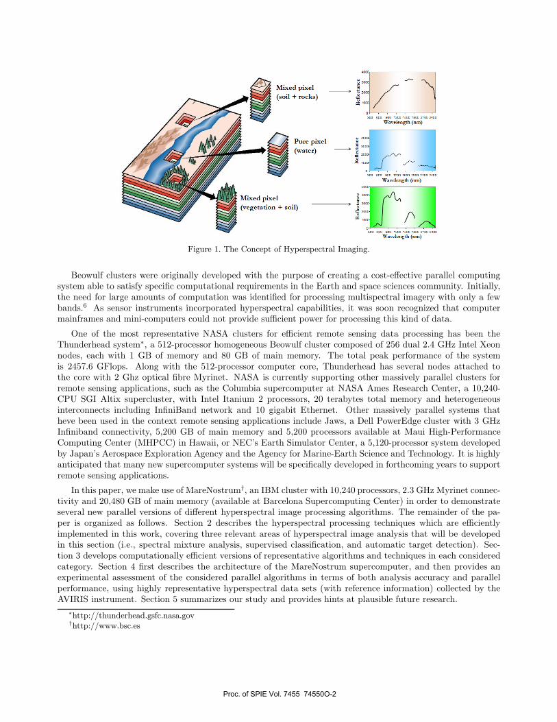
Figure 1. The Concept of Hyperspectral Imaging.

Beowulf clusters were originally developed with the purpose of creating a cost-effective parallel computingsystem able to satisfy specific computational requirements in the Earth and space sciences community. Initially,the need for large amounts of computation was identified for processing multispectral imagery with only a fewbands.6 As sensor instruments incorporated hyperspectral capabilities, it was soon recognized that computermainframes and mini-computers could not provide sufficient power for processing this kind of data.

One of the most representative NASA clusters for efficient remote sensing data processing has been theThunderhead system∗, a 512-processor homogeneous Beowulf cluster composed of 256 dual 2.4 GHz Intel Xeonnodes, each with 1 GB of memory and 80 GB of main memory. The total peak performance of the systemis 2457.6 GFlops. Along with the 512-processor computer core, Thunderhead has several nodes attached tothe core with 2 Ghz optical fibre Myrinet. NASA is currently supporting other massively parallel clusters forremote sensing applications, such as the Columbia supercomputer at NASA Ames Research Center, a 10,240-CPU SGI Altix supercluster, with Intel Itanium 2 processors, 20 terabytes total memory and heterogeneousinterconnects including InfiniBand network and 10 gigabit Ethernet. Other massively parallel systems thatheve been used in the context remote sensing applications include Jaws, a Dell PowerEdge cluster with 3 GHzInfiniband connectivity, 5,200 GB of main memory and 5,200 processors available at Maui High-PerformanceComputing Center (MHPCC) in Hawaii, or NEC’s Earth Simulator Center, a 5,120-processor system developedby Japan’s Aerospace Exploration Agency and the Agency for Marine-Earth Science and Technology. It is highlyanticipated that many new supercomputer systems will be specifically developed in forthcoming years to supportremote sensing applications.

In this paper, we make use of MareNostrum†, an IBM cluster with 10,240 processors, 2.3 GHz Myrinet connec-tivity and 20,480 GB of main memory (available at Barcelona Supercomputing Center) in order to demonstrateseveral new parallel versions of different hyperspectral image processing algorithms. The remainder of the pa-per is organized as follows. Section 2 describes the hyperspectral processing techniques which are efficientlyimplemented in this work, covering three relevant areas of hyperspectral image analysis that will be developedin this section (i.e., spectral mixture analysis, supervised classification, and automatic target detection). Sec-tion 3 develops computationally efficient versions of representative algorithms and techniques in each consideredcategory. Section 4 first describes the architecture of the MareNostrum supercomputer, and then provides anexperimental assessment of the considered parallel algorithms in terms of both analysis accuracy and parallelperformance, using highly representative hyperspectral data sets (with reference information) collected by theAVIRIS instrument. Section 5 summarizes our study and provides hints at plausible future research.

∗http://thunderhead.gsfc.nasa.gov†http://www.bsc.es


2. METHODS

2.1 Spectral mixture analysis

Spectral unmixing has been an alluring exploitation goal since the earliest days of imaging spectroscopy.7 Nomatter the spatial resolution in natural environments, spectral signatures in hyperspectral data are invariably amixture of the signatures of the various materials found within the spatial extent of the ground instantaneousfield view (see Fig. 1). Due to the high spectral dimensionality of the data, the number of spectral bandsusually exceeds the number of spectral mixture components, and the unmixing problem is cast in terms of anover-determined system of equations in which, given a correct set of pure spectral signatures called endmem-bers ,8 the objective is to estimate fractional abundances for those endmembers. Since each observed spectralsignal is the result of an actual mixing process, the driving abundances must obey two rather common-senseconstraints. First, all abundances must be non-negative. Second, the sum of abundances for a given pixel mustbe unity. However, it is the derivation and validation of the correct suite of endmembers that has remained achallenging and elusive goal for the past twenty years. Over the last years, several algorithms have been devel-oped for automatic or semi-automatic extraction of spectral endmembers directly from an input hyperspectraldata set. Some classic techniques for this purpose include the pixel purity index (PPI)9 or the N-FINDR algo-rithm,10 both focused on analyzing the data without incorporating information on the spatially adjacent data.However, one of the distinguishing properties of hyperspectral data is the multivariate information coupled witha two-dimensional (pictorial) representation amenable to image interpretation. In this work, we address thecomputational requirements introduced by spectral unmixing applications by addressing a specific case studyfocused on efficient implementation of the automatic morphological endmember extraction (AMEE) algorithm,11

a technique that integrates both the spatial and the spectral information when searching for image endmembersin hyperspectral data sets.

2.2 Supervised classification

The utilization of fully or partially unsupervised approaches, such as the spectral unmixing techniques discussedin the previous subsection, are of great interest for extracting relevant information from hyperspectral scenes.However, several machine learning and image processing techniques have also been applied for the same purposewhen a priori knowledge (often available in the form of labeled data or ground-truth) is available for the scenesto be analyzed.12 In this case, the labeled data usually consists of training samples cataloged by assuming thateach pixel vector measures the response of one single underlying material. Perhaps the most relevant examples ofsupervised machine learning techniques used for remote sensing data classification are support vector machines(SVMs)13 and artificial neural networks.14 Although many neural network architectures exist, for hyperspectraldata classification mostly feed-forward networks of various layers, such as the multi-layer perceptron (MLP), havebeen used.15 In this work, the computational requirements addressed by supervised classifiers are illustrated bya case study focused on efficient implementation of an MLP-based classifier for hyperspectral image data.

2.3 Automatic target detection

Another technique that has attracted a lot of attention in hyperspectral image analysis in recent years is automatictarget detection,16 which is particularly crucial in military-oriented applications. During the last few years,several algorithms have been developed for the aforementioned purpose, including the automatic target detectionand classification (ATDCA) algorithm,17 an unsupervised fully-constrained least squares (UFCLS) algorithm,18

an iterative error analysis (IEA) algorithm,19 or the well-known RX algorithm developed by Reed and Xiaoli foranomaly detection.20 In this work, we illustrate the computational requirements of target detection applicationsby addressing a case study focused on efficient implementation of the ATDCA algorithm.

In the following section, we describe parallel versions of ATDCA for target detection, AMEE for endmemberextraction, and MLP for supervised classification of hyperspectral data. We believe that, although additionalimplementation case studies would be certainly relevant, the spectrum of parallel techniques included in thispaper provides sufficient coverage of different strategies and approaches for efficient information extraction fromhyperspectral data sets.


3. PARALLEL IMPLEMENTATIONS

In all considered parallel implementations, a data-driven partitioning strategy has been adopted as a baselinefor algorithm parallelization. Specifically, two approaches for data partitioning have been tested:5

• Spectral-domain partitioning. This approach subdivides the multi-channel remotely sensed image into smallcells or sub-volumes made up of contiguous spectral wavelengths for parallel processing.

• Spatial-domain partitioning. This approach breaks the multi-channel image into slices made up of oneor several contiguous spectral bands for parallel processing. In this case, the same pixel vector is alwaysentirely assigned to a single processor, and slabs of spatially adjacent pixel vectors are distributed amongthe processing nodes (CPUs) of the parallel system.

Previous experimentation with the above-mentioned strategies indicated that spatial-domain partitioningcan significantly reduce inter-processor communication, resulting from the fact that a single pixel vector is neverpartitioned and communications are not needed at the pixel level.5 In the following, we assume that spatial-domain decomposition is always used when partitioning the hyperspectral data cube.

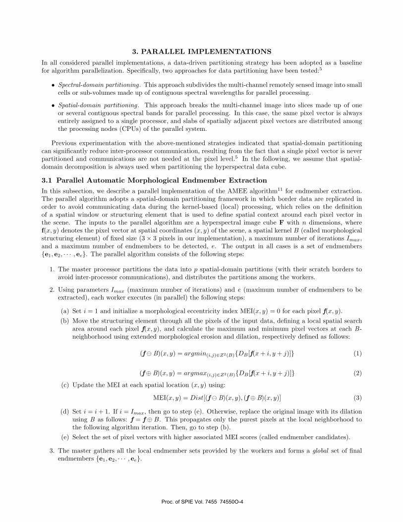
3.1 Parallel Automatic Morphological Endmember ExtractionIn this subsection, we describe a parallel implementation of the AMEE algorithm11 for endmember extraction.The parallel algorithm adopts a spatial-domain partitioning framework in which border data are replicated inorder to avoid communicating data during the kernel-based (local) processing, which relies on the definitionof a spatial window or structuring element that is used to define spatial context around each pixel vector inthe scene. The inputs to the parallel algorithm are a hyperspectral image cube F with n dimensions, wheref(x, y) denotes the pixel vector at spatial coordinates (x, y) of the scene, a spatial kernel B (called morphologicalstructuring element) of fixed size (3 × 3 pixels in our implementation), a maximum number of iterations Imax,and a maximum number of endmembers to be detected, e. The output in all cases is a set of endmembers{e1, e2, · · · , ee}. The parallel algorithm consists of the following steps:

1. The master processor partitions the data into p spatial-domain partitions (with their scratch borders toavoid inter-processor communications), and distributes the partitions among the workers.

2. Using parameters Imax (maximum number of iterations) and e (maximum number of endmembers to beextracted), each worker executes (in parallel) the following steps:

(a) Set i = 1 and initialize a morphological eccentricity index MEI(x, y) = 0 for each pixel f(x, y).(b) Move the structuring element through all the pixels of the input data, defining a local spatial search

area around each pixel f(x, y), and calculate the maximum and minimum pixel vectors at each B -neighborhood using extended morphological erosion and dilation, respectively defined as follows:

(f� B)(x, y) = argmin(i,j)∈Z2(B){DB[f(x + i, y + j)]} (1)

(f⊕ B)(x, y) = argmax(i,j)∈Z2(B){DB[f(x + i, y + j)]} (2)

(c) Update the MEI at each spatial location (x, y) using:

MEI(x, y) = Dist[(f� B)(x, y), (f ⊕ B)(x, y)] (3)

(d) Set i = i + 1. If i = Imax, then go to step (e). Otherwise, replace the original image with its dilationusing B as follows: f = f ⊕ B. This propagates only the purest pixels at the local neighborhood tothe following algorithm iteration. Then, go to step (b).

(e) Select the set of pixel vectors with higher associated MEI scores (called endmember candidates).

3. The master gathers all the local endmember sets provided by the workers and forms a global set of finalendmembers {e1, e2, · · · , ee}.


3.2 Parallel Multi-Layer Perceptron

In this subsection, we describe a supervised parallel classifier based on a MLP neural network with back-propagation learning.15 The inputs to the parallel algorithm are a hyperspectral image cube F with n dimensions,where f(x, y) denotes the pixel vector at spatial coordinates (x, y) of the scene. The number of input neurons ofthe considered neural network equals n, the number of spectral bands acquired by the sensor. The number ofhidden neurons, m, is adjusted empirically, and the number of output neurons, c, equals the number of distinctclasses to be identified in the input data.

The parallel classifier considered in this work is based on an exemplar partitioning scheme, also called trainingexample parallelism, which explores data level parallelism and can be easily obtained by simply partitioning thetraining pattern data set. Each process determines the weight changes for a disjoint subset of the trainingpopulation and then changes are combined and applied to the neural network at the end of each epoch. Thisscheme requires a suitable large number of training patterns to take an advantage. Each processor implementsa complete neural network which is trained with a disjoint subset of training patterns fpj (x, y)), executing thefollowing three phases of the back-propagation learning algorithm for each training pattern:

1. Parallel forward phase. In this phase, the activation value of the hidden neurons local to the processorsare calculated. For each input pattern –meaning that labeled pixel vectors are used as training patterns–the activation value for the hidden neurons is calculated at each processor using the expression Hp

i =ϕ(

∑nj=1 ωij · fpj (x, y)). Here, the activation values and weight connections of neurons present in other

processors are required to calculate the activation values of output neurons according to the expressionOP

k = ϕ(∑m

i=1 ωpki · Hp

i ), with k = 1, 2, · · · , C.

2. Parallel error back-propagation. In this phase, each processor calculates the error terms for the local hiddenneurons. To do so, delta terms for the output neurons are first calculated using (δo

k)P = (Ok − dk)p ·ϕ′(·),

with i = 1, 2, · · · , c. Then, error terms for the hidden layer are computed using the following expression:(δh

i )p =∑p

k=1(ωpki · (δo

k)p) · ϕ′(·), with i = 1, 2, · · · , n.

3. Parallel weight update. In this phase, the weight connections between the input and hidden layers areupdated by ωij = ωij + ηp · (δh

i )p · fpj (x, y)). Similarly, the weight connections between the hidden andoutput layers are updated using the expression: ωp

ki = ωPki + ηp · (δo

k)p · Hpi .

4. Broadcast and initialization of weight matrices. In this phase, each node sends its partial weight matricesto its neighbour node, which sums it to its partial matrix and proceed to send it again to the neighbour.Once all nodes have added their local matrices the resulting total weight matrices are broadcast to be usedby all processors in the next iteration.

Once the MLP neural network has been trained with a set of labeled patterns, a parallel classification stepfollows. For each pixel vector f(x, y) in the input data cube, the classification step calculates (in parallel)∑p

j=1 Ojk, with k = 1, 2 · · · , c. A classification label for each pixel can be obtained using the winner-take-all

criterion commonly used in neural networks by finding the cumulative sum with maximum value, say∑p

j=1 Ojk∗ ,

with k∗ = arg{max1≤k≤c

∑pj=1 Oj

k}.

3.3 Parallel Automatic Target Detection and Classification Algorithm

In this subsection, we describe a parallel implementation of the ATDCA algorithm17 for automatic target detec-tion. The inputs to the parallel algorithm are a hyperspectral image cube F with n dimensions, where f denotesa pixel vector at spatial coordinates (x, y) of the scene, and a maximum number of targets to be detected, t. Theoutput in all cases is a set of target pixel vectors {t0, t1, · · · , tt}. The parallel algorithm consists of the followingsteps:

1. The master divides the original image cube F into p spatial-domain partitions. Then, the master sends thepartitions to the workers.


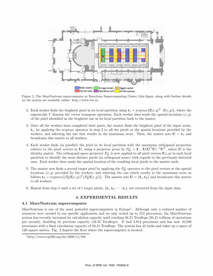
Figure 2. The MareNostrum supercomputer at Barcelona Supercomputing Center (this figure, along with further detailson the system are available online: http://www.bsc.es.

2. Each worker finds the brightest pixel in its local partition using t1 = argmax{f(x, y)T · f(x, y)}, where thesuperscript T denotes the vector transpose operation. Each worker then sends the spatial locations (x, y)of the pixel identified as the brightest one in its local partition back to the master.

3. Once all the workers have completed their parts, the master finds the brightest pixel of the input scene,t1, by applying the argmax operator in step 2 to all the pixels at the spatial locations provided by theworkers, and selecting the one that results in the maximum score. Then, the master sets U = t1 andbroadcasts this matrix to all workers.

4. Each worker finds (in parallel) the pixel in its local partition with the maximum orthogonal projectionrelative to the pixel vectors in U, using a projector given by P⊥

U = I − U(UTU)−1UT , where U is theidentity matrix. The orthogonal space projector P⊥

U is now applied to all pixel vectors f(x, y) in each localpartition to identify the most distinct pixels (in orthogonal sense) with regards to the previously detectedones. Each worker then sends the spatial location of the resulting local pixels to the master node.

5. The master now finds a second target pixel by applying the P⊥U operator to the pixel vectors at the spatial

locations (x, y) provided by the workers, and selecting the one which results in the maximum score asfollows t2 = argmax{(P⊥

U f(x, y))T (P⊥U f(x, y))}. The master sets U = {t1, t2} and broadcasts this matrix

to all workers.

6. Repeat from step 4 until a set of t target pixels, {t1, t2, · · · , tt}, are extracted from the input data.

4. EXPERIMENTAL RESULTS

4.1 MareNostrum supercomputer

MareNostrum is one of the most powerful supercomputers in Europe‡. Although only a reduced number ofresources were needed in our specific application and we only scaled up to 512 processors, the MareNostrumsystem has recently increased its calculation capacity until reaching 94.21 Teraflops (94.21 trillions of operationsper second), doubling its previous capacity (42.35 Teraflops). It had 4.812 processors and has now 10.240processors with a final calculation capacity of 94.21 Teraflops. The system has 44 racks and takes up a space of120 square meters. Fig. 2 depicts the floor where the supercomputer is located.

‡http://www.top500.org/list/2008/11/100


4.2 Hyperspectral images

Three hyperspectral scenes collected by the AVIRIS instrument have been used in experiments:

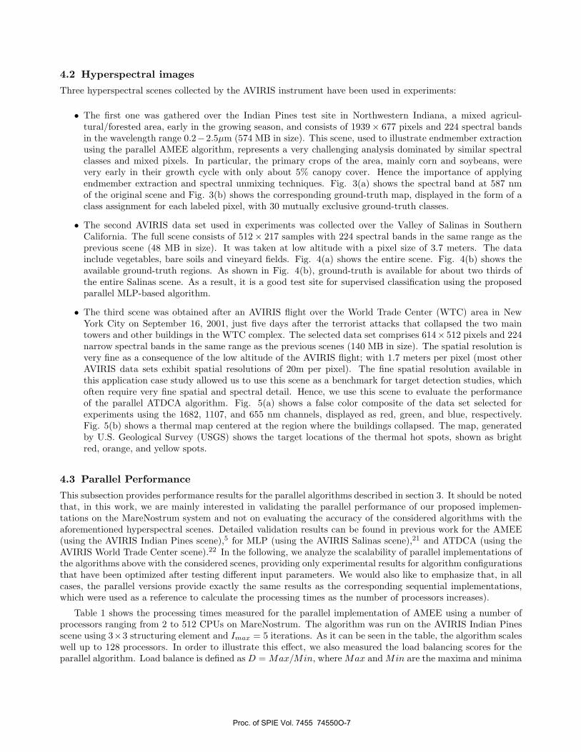
• The first one was gathered over the Indian Pines test site in Northwestern Indiana, a mixed agricul-tural/forested area, early in the growing season, and consists of 1939× 677 pixels and 224 spectral bandsin the wavelength range 0.2−2.5μm (574 MB in size). This scene, used to illustrate endmember extractionusing the parallel AMEE algorithm, represents a very challenging analysis dominated by similar spectralclasses and mixed pixels. In particular, the primary crops of the area, mainly corn and soybeans, werevery early in their growth cycle with only about 5% canopy cover. Hence the importance of applyingendmember extraction and spectral unmixing techniques. Fig. 3(a) shows the spectral band at 587 nmof the original scene and Fig. 3(b) shows the corresponding ground-truth map, displayed in the form of aclass assignment for each labeled pixel, with 30 mutually exclusive ground-truth classes.

• The second AVIRIS data set used in experiments was collected over the Valley of Salinas in SouthernCalifornia. The full scene consists of 512 × 217 samples with 224 spectral bands in the same range as theprevious scene (48 MB in size). It was taken at low altitude with a pixel size of 3.7 meters. The datainclude vegetables, bare soils and vineyard fields. Fig. 4(a) shows the entire scene. Fig. 4(b) shows theavailable ground-truth regions. As shown in Fig. 4(b), ground-truth is available for about two thirds ofthe entire Salinas scene. As a result, it is a good test site for supervised classification using the proposedparallel MLP-based algorithm.

• The third scene was obtained after an AVIRIS flight over the World Trade Center (WTC) area in NewYork City on September 16, 2001, just five days after the terrorist attacks that collapsed the two maintowers and other buildings in the WTC complex. The selected data set comprises 614× 512 pixels and 224narrow spectral bands in the same range as the previous scenes (140 MB in size). The spatial resolution isvery fine as a consequence of the low altitude of the AVIRIS flight; with 1.7 meters per pixel (most otherAVIRIS data sets exhibit spatial resolutions of 20m per pixel). The fine spatial resolution available inthis application case study allowed us to use this scene as a benchmark for target detection studies, whichoften require very fine spatial and spectral detail. Hence, we use this scene to evaluate the performanceof the parallel ATDCA algorithm. Fig. 5(a) shows a false color composite of the data set selected forexperiments using the 1682, 1107, and 655 nm channels, displayed as red, green, and blue, respectively.Fig. 5(b) shows a thermal map centered at the region where the buildings collapsed. The map, generatedby U.S. Geological Survey (USGS) shows the target locations of the thermal hot spots, shown as brightred, orange, and yellow spots.

4.3 Parallel Performance

This subsection provides performance results for the parallel algorithms described in section 3. It should be notedthat, in this work, we are mainly interested in validating the parallel performance of our proposed implemen-tations on the MareNostrum system and not on evaluating the accuracy of the considered algorithms with theaforementioned hyperspectral scenes. Detailed validation results can be found in previous work for the AMEE(using the AVIRIS Indian Pines scene),5 for MLP (using the AVIRIS Salinas scene),21 and ATDCA (using theAVIRIS World Trade Center scene).22 In the following, we analyze the scalability of parallel implementations ofthe algorithms above with the considered scenes, providing only experimental results for algorithm configurationsthat have been optimized after testing different input parameters. We would also like to emphasize that, in allcases, the parallel versions provide exactly the same results as the corresponding sequential implementations,which were used as a reference to calculate the processing times as the number of processors increases).

Table 1 shows the processing times measured for the parallel implementation of AMEE using a number ofprocessors ranging from 2 to 512 CPUs on MareNostrum. The algorithm was run on the AVIRIS Indian Pinesscene using 3×3 structuring element and Imax = 5 iterations. As it can be seen in the table, the algorithm scaleswell up to 128 processors. In order to illustrate this effect, we also measured the load balancing scores for theparallel algorithm. Load balance is defined as D = Max/Min, where Max and Min are the maxima and minima


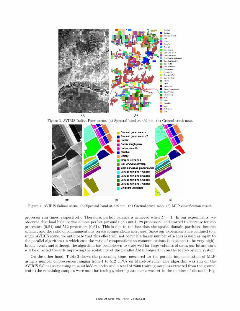
Figure 3. AVIRIS Indian Pines scene. (a) Spectral band at 439 nm. (b) Ground-truth map.

Figure 4. AVIRIS Salinas scene. (a) Spectral band at 439 nm. (b) Ground-truth map. (c) MLP classification result.

processor run times, respectively. Therefore, perfect balance is achieved when D = 1. In our experiments, weobserved that load balance was almost perfect (around 0.99) until 128 processors, and started to decrease for 256processors (0.84) and 512 processors (0.61). This is due to the fact that the spatial-domain partitions becomesmaller, and the ratio of communications versus computations increases. Since our experiments are confined to asingle AVIRIS scene, we anticipate that this effect will not occur if a larger number of scenes is used as input tothe parallel algorithm (in which case the ratio of computations to communications is expected to be very high).In any event, and although the algorithm has been shown to scale well for large volumes of data, our future workwill be directed towards improving the scalability of the parallel AMEE algorithm on the MareNostrum system.

On the other hand, Table 2 shows the processing times measured for the parallel implementation of MLPusing a number of processors ranging from 4 to 512 CPUs on MareNostrum. The algorithm was run on theAVIRIS Salinas scene using m = 40 hidden nodes and a total of 2500 training samples extracted from the groundtruth (the remaining samples were used for testing), where parameter c was set to the number of classes in Fig.


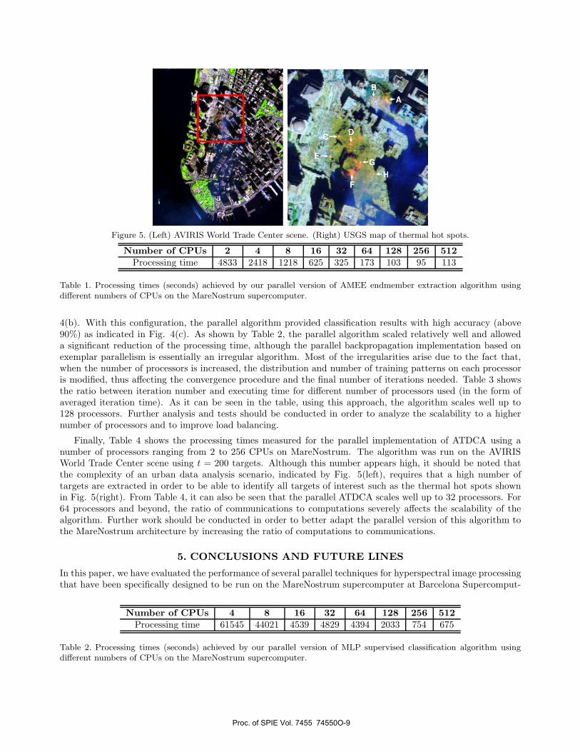
Figure 5. (Left) AVIRIS World Trade Center scene. (Right) USGS map of thermal hot spots.

Number of CPUs 2 4 8 16 32 64 128 256 512Processing time 4833 2418 1218 625 325 173 103 95 113

Table 1. Processing times (seconds) achieved by our parallel version of AMEE endmember extraction algorithm usingdifferent numbers of CPUs on the MareNostrum supercomputer.

4(b). With this configuration, the parallel algorithm provided classification results with high accuracy (above90%) as indicated in Fig. 4(c). As shown by Table 2, the parallel algorithm scaled relatively well and alloweda significant reduction of the processing time, although the parallel backpropagation implementation based onexemplar parallelism is essentially an irregular algorithm. Most of the irregularities arise due to the fact that,when the number of processors is increased, the distribution and number of training patterns on each processoris modified, thus affecting the convergence procedure and the final number of iterations needed. Table 3 showsthe ratio between iteration number and executing time for different number of processors used (in the form ofaveraged iteration time). As it can be seen in the table, using this approach, the algorithm scales well up to128 processors. Further analysis and tests should be conducted in order to analyze the scalability to a highernumber of processors and to improve load balancing.

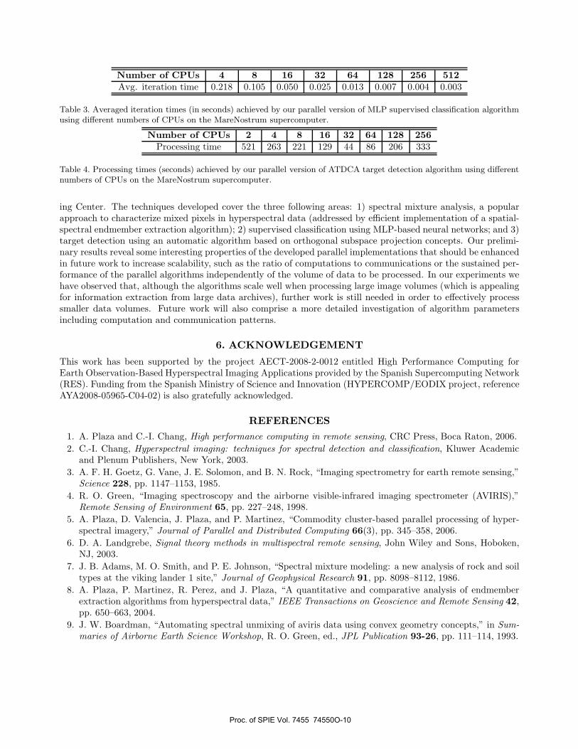
Finally, Table 4 shows the processing times measured for the parallel implementation of ATDCA using anumber of processors ranging from 2 to 256 CPUs on MareNostrum. The algorithm was run on the AVIRISWorld Trade Center scene using t = 200 targets. Although this number appears high, it should be noted thatthe complexity of an urban data analysis scenario, indicated by Fig. 5(left), requires that a high number oftargets are extracted in order to be able to identify all targets of interest such as the thermal hot spots shownin Fig. 5(right). From Table 4, it can also be seen that the parallel ATDCA scales well up to 32 processors. For64 processors and beyond, the ratio of communications to computations severely affects the scalability of thealgorithm. Further work should be conducted in order to better adapt the parallel version of this algorithm tothe MareNostrum architecture by increasing the ratio of computations to communications.

5. CONCLUSIONS AND FUTURE LINES

In this paper, we have evaluated the performance of several parallel techniques for hyperspectral image processingthat have been specifically designed to be run on the MareNostrum supercomputer at Barcelona Supercomput-

Number of CPUs 4 8 16 32 64 128 256 512Processing time 61545 44021 4539 4829 4394 2033 754 675

Table 2. Processing times (seconds) achieved by our parallel version of MLP supervised classification algorithm usingdifferent numbers of CPUs on the MareNostrum supercomputer.


Number of CPUs 4 8 16 32 64 128 256 512Avg. iteration time 0.218 0.105 0.050 0.025 0.013 0.007 0.004 0.003

Table 3. Averaged iteration times (in seconds) achieved by our parallel version of MLP supervised classification algorithmusing different numbers of CPUs on the MareNostrum supercomputer.

Number of CPUs 2 4 8 16 32 64 128 256Processing time 521 263 221 129 44 86 206 333

Table 4. Processing times (seconds) achieved by our parallel version of ATDCA target detection algorithm using differentnumbers of CPUs on the MareNostrum supercomputer.

ing Center. The techniques developed cover the three following areas: 1) spectral mixture analysis, a popularapproach to characterize mixed pixels in hyperspectral data (addressed by efficient implementation of a spatial-spectral endmember extraction algorithm); 2) supervised classification using MLP-based neural networks; and 3)target detection using an automatic algorithm based on orthogonal subspace projection concepts. Our prelimi-nary results reveal some interesting properties of the developed parallel implementations that should be enhancedin future work to increase scalability, such as the ratio of computations to communications or the sustained per-formance of the parallel algorithms independently of the volume of data to be processed. In our experiments wehave observed that, although the algorithms scale well when processing large image volumes (which is appealingfor information extraction from large data archives), further work is still needed in order to effectively processsmaller data volumes. Future work will also comprise a more detailed investigation of algorithm parametersincluding computation and communication patterns.

6. ACKNOWLEDGEMENT

This work has been supported by the project AECT-2008-2-0012 entitled High Performance Computing forEarth Observation-Based Hyperspectral Imaging Applications provided by the Spanish Supercomputing Network(RES). Funding from the Spanish Ministry of Science and Innovation (HYPERCOMP/EODIX project, referenceAYA2008-05965-C04-02) is also gratefully acknowledged.

REFERENCES1. A. Plaza and C.-I. Chang, High performance computing in remote sensing, CRC Press, Boca Raton, 2006.2. C.-I. Chang, Hyperspectral imaging: techniques for spectral detection and classification, Kluwer Academic

and Plenum Publishers, New York, 2003.3. A. F. H. Goetz, G. Vane, J. E. Solomon, and B. N. Rock, “Imaging spectrometry for earth remote sensing,”

Science 228, pp. 1147–1153, 1985.4. R. O. Green, “Imaging spectroscopy and the airborne visible-infrared imaging spectrometer (AVIRIS),”

Remote Sensing of Environment 65, pp. 227–248, 1998.5. A. Plaza, D. Valencia, J. Plaza, and P. Martinez, “Commodity cluster-based parallel processing of hyper-

spectral imagery,” Journal of Parallel and Distributed Computing 66(3), pp. 345–358, 2006.6. D. A. Landgrebe, Signal theory methods in multispectral remote sensing, John Wiley and Sons, Hoboken,

NJ, 2003.7. J. B. Adams, M. O. Smith, and P. E. Johnson, “Spectral mixture modeling: a new analysis of rock and soil

types at the viking lander 1 site,” Journal of Geophysical Research 91, pp. 8098–8112, 1986.8. A. Plaza, P. Martinez, R. Perez, and J. Plaza, “A quantitative and comparative analysis of endmember

extraction algorithms from hyperspectral data,” IEEE Transactions on Geoscience and Remote Sensing 42,pp. 650–663, 2004.

9. J. W. Boardman, “Automating spectral unmixing of aviris data using convex geometry concepts,” in Sum-maries of Airborne Earth Science Workshop, R. O. Green, ed., JPL Publication 93-26, pp. 111–114, 1993.


10. M. E. Winter, “Algorithm for fast autonomous spectral endmember determination in hyperspectral data,”in Imaging Spectrometry V, M. R. Descour and S. S. Shen, eds., Proceedings of SPIE 3753, pp. 266–275,1999.

11. A. Plaza, P. Martinez, R. Perez, and J. Plaza, “Spatial/spectral endmember extraction by multidimensionalmorphological operations,” IEEE Transactions on Geoscience and Remote Sensing 40, pp. 2025–2041, 2002.

12. G. M. Foody and A. Mathur, “Toward intelligent training of supervised image classifications: directingtraining data acquisition for svm classification,” Remote Sensing of Environment 93, pp. 107–117, 2004.

13. L. Bruzzone, M. Chi, and M. Marconcini, “A novel transductive svm for the semisupervised classificationof remote sensing images,” IEEE Trans. Geoscience and Remote Sensing 44, pp. 3363–3373, 2006.

14. C. Lee and D. A. Landgrebe, “Decision boundary feature extraction for neural networks,” IEEE Trans.Neural Networks 8, pp. 75–83, 1997.

15. J. Plaza, A. Plaza, R. Perez, and P. Martinez, “On the use of small training sets for neural network-based characterization of mixed pixels in remotely sensed hyperspectral images,” Pattern Recognition 42,pp. 3032–3045, 2009.

16. D. Manolakis, D. Marden, and G. A. Shaw, “Hyperspectral image processing for automatic target detectionapplications,” MIT Lincoln Laboratory Journal 14, pp. 79–116, 2003.

17. H. Ren and C.-I. Chang, “Automatic spectral target recognition in hyperspectral imagery,” IEEE Trans.Aerosp. Electron. Syst. 39, pp. 1232–1249, 2003.

18. D. Heinz and C.-I. Chang, “Fully constrained least squares linear mixture analysis for material quantificationin hyperspectral imagery,” IEEE Trans. Geosci. Remote Sens. 39, pp. 529–545, 2001.

19. R. A. Neville, K. Staenz, T. Szeredi, J. Lefebvre, and P. Hauff, “Automatic endmember extraction fromhyperspectral data for mineral exploration,” in 21st Canadian Symposium on Remote Sensing, pp. 401–415,1999.

20. I. Reed and X.Yu, “Adaptive multiple-band cfar detection of an optical pattern with unknown spectraldistrihution.,” IEEE Trans. Acoustics, Speech and Signal Processing 38, pp. 1760–1770, 1990.

21. J. Plaza, R. Perez, A. Plaza, P. Martinez, and D. Valencia, “Parallel morphological/neural processing ofhyperspectral images using heterogeneous and homogeneous platforms,” Cluster Computing 11, pp. 17–32,2008.

22. A. Paz, A. Plaza, and S. Blazquez, “Parallel implementation of target detection algorithms for hyperspectralimagery,” Proceedings of the IEEE International Geoscience and Remote Sensing Symposium 1, pp. 234–239–32, 2008.


Massively parallel processing of remotely sensed ... · Massively Parallel Processing of Remotely...

Documents

Transcript of Massively parallel processing of remotely sensed ... · Massively Parallel Processing of Remotely...