Massively Parallel, Adaptive, Color Image Processing for

Massively Parallel, Adaptive, Color Image Processing for Autonomous Road Following

Todd Jochem and Shumeet Baluja

CMU-RI-TR-93- 10

The Robotics Institute and Department of Computer Science Carnegie Mellon University

Pittsburgh, Pennsylvania 15213

May 1993

@ 1993 Camegie Mellon University

This research was partly sponsored by DARPA, under contracts “Perception for Outdoor Navigation” (contract number DACA76-89-C-0014, monitored by the US Army Topo- graphic Engineering Center) and “Unmanned Ground Vehicle System” (contract number DAAE07-90-C-R059, monitored by TACOM) as well as a DARPA Research Assistant- ship in Parallel Processing administered by the Institute for Advanced Computer Studies, University pf Maryland. Additionally, the MasPar MP-1 at the Parallel Processing Lab at Purdue University was funded through NSF award number CDA-9015696.

The views and conclusions contained in this document are those of the authors and should not be interpreted as representing the official policies, either expressed or implied, of the U.S. government.

Massively Parallel, Adaptive, Color Image Processing for Autonomous Road Following

1. Introduction

2. Overview of System

3. The Clustering Algorithm

4. The Combining Algorithm

5. The Road Finding Algorithm

6. Runtime Processing

7. Results

8. Other Related Systems

9. Future Work

10. Conclusions

11. Acknowledgments

Appendix A: Competitive Learning

Appendix B: Artificial Neural Networks

Appendix C: Hough Transform

Appendix D: Alternative Pixel Averaging

Appendix E: The MasPar MP-1

Appendix F: MasPar Programming Language

1

1

3

9

12

15

15

17

17

18

19

19

20

21

22

23

24

Abstract In recent years, significant progress has been made towards achieving autonomous roadway navigation using video images. None of these systems take full advantage of all the information i n the 5 12x512 pixel frame, 30 framdsecond color image sequence. This can be attributed to the large m o u n t of data which is present in the color video image stream (22.5 Mbyteslsec) as well as the limited amount of computing resources available to the systems. We have increased the available computing power by using a parallel computer. Specifically. a single instruction, multiple data (SIMD) machine was used to develop simple and efficient parallel algorithms. largely based on connectionist techniques, which can process every pixel in the incoming 30 framdsecond. color video image stream, The system uses substantially larger frames and processes them at faster rates than other color road following systems. This is achievable through the use of algorithms specifically designed for a fine-grained parallel machine as opposed to ones ported frnm existing systems to parallel architectures. The algorithms presented here were tested on 4k and 16k processor MasPar MP-1 and on 4K, XK. and I6K processor MasPar MP-2 parallel machines and were used to drive CamegieMellon's testbed vehicle, the Navlab I, on paved roads near campus.

1. Introduction

I n the pact few years, the systems designed for autonomous roadway navigation using video images have relied on a wide variety ofdifferent techniques [Thorpe, 1990). The techniques range from neural network architectures that learn the appropriate road features required for driving [Pomerleau, 19911. to systems which find road lines and edges based on predefined road models [Kluge, 19921. Many of these systems have been able to drive vehicles at high speeds. in traffic, and on real highways. However. none of these systems have been able to use all of the information present in 512 x 512 input images. This can be attributed to the limited computing power available to the systems in the face of the sheer magnitude of data being presented to them (22.5 Mbyteslsec).

Several methods can be used to handle these large sets of data which occur in road following tasks. Onc method is to use grayscale images instead of color images. Grayscale images cut the amount of data which must be processed by two-thirds. However, eve.n at this lower data rate. processing every pixel is still extremely diEficult? and subsampling LCrisman, 19901 and windowing techniques [Turk, 19881 are frequently used to try to achieve frame rate processing on the incoming color data. Another method is to preprocess the color image, projecting the 3D color data into a single value at each pixel [Turk, 19881. This method, like windowing, has the desired effect of reducing the amount of data which must be processed by the system. Defining regions of interest and only processing the pixels within them is another possibility and has been explored by [Kluge, 19921 and [Dickmanns, 19921. A final method, and the method we chose to use. is to increase the available computing power by using a massively parallel, single instruction, multiple data (SIMD) computer. The system uses substantially larger frames and pmcesses them at faster rates than other color road following systems. The improved rates are achieved through the use of algorithms specifically designed for a finegrained parallel machine. Although higher resolution does not directly lead to increased driving accuracy, systems which can handle these resolutions at faster rates have a clear advantage in other domains were fine features are more important. It is our hope that the rudimentary algorithms presented in this paper can be extend to other such vision tasks.

2. Overview of System

As is the case in nearly all vision system, a number of assumptions have been made about the environment to simplify the problem. The assumptions relate to the mad model, operating conditions, and available sensors. Two assumptions which our system makes are the defining road model. and the relationship between the colors in each scene and their placements within the color space. These assumptions will be described in greater detail i n the upcoming paragraphs.

The first assumption is that of a trapezoidal road model. In this model, the road is described in the image as a region bounded by four edges. Two of these edges are defined as the location where road and non-road meet while the other two are the top and bottom of the image itself. These four edges constitute the trapezoid. The road center line is defined to be the geometric line which bisech the trapezoid vertically. For a graphic representation of this model see Figure 1. In addition, our system assumes that the road remains a constant width through all of the input images. This constraint means that although the trapezoid of the mad may be skewed to the left or right. the top and bottom edges remain a constant length. As the lookahead in our camera is small, this assumption does not hinder performance. This issue will be returned to later.

Color clusters play an important role in our system. A color cluster is defined a the group of pixels in the 3D (red, green. blue) color space which are closest to a particular central, or mean, pixel value. In our representation, closeness is defined by the sum of squared difference between a pixel's red, green, and blue values and a central pixel's red, green. and blue values.

An assumption based on this concept is that the colors in the image can be adequately represented. or classified. by a small (between 5 and 30) number of clusters. In our system, the ability of a set of clusters to classify an image is measured by how well the mean values of the clusters of the set can reconstruct the original input image. This will be discussed further in section 3.2. Our final assumption is that any particular cluster can only correctly classify pixels i n the road or the non-road portions of the image; it cannot correctly classify pixels in both.

2

Trapezoidal road model superimposed on image.

Road center line.

RoadfNon-Road edge.

Road

Non-Road

Figure 1. Trapezoidal mad model.

Because the mad and non-road pixels of typical road images, when plotted in color space. form largely disjoint sets. and because of the nature of the algorithm which partitions color space into clusters, this has proven to be a reasonable assumption. (See Figure 4.)

The system we have developed is an iterative, three step procedure in which evety pixel in the input image is classified by a color cluster, labeled as road or non-road, and then used to find the center l ine of the road. The world coordinates of this line are passed to the vehicle controller which guides the vehicle on the specified path. This process is supplemented by an initialization phase which occurs only once on the initial image the system processes. A high level view of the system architecture is shown in Figure 2.

This system is pixel driven; thus all computation can be done very efficiently on a massively parallel processor array. lnstead of mapping existing road following algorithms to the processor array, we integrated algorithms which could exploit the tightly coupled processor array and take advantage of the limited capabilities of the individual processors. The resulting system is fully parallelized, and performs comparably to the state-of-the-art.

Our system is composed of three main algorithms, all of which are parallelized on the processor array. The three parts are a clustering algorithm, a combining algorithm. and a road finding algorithm. The clustering algorithm is an iterative procedure which uses a parallel competitive learning implementation of the isodata clustering algorithm [Ball, 19671 to find the mean red, green. and blue values for each color cluster i n the input image. This will be described in greater detail in the next section.

The combining algorithm is a single perceptron which is trained to correctly determine whether a pixel in the input image is a road pixel or an non-road pixel. This is accomplished by using information derived from classification of the pixel using the means developed in the clustering algorithm. The clustering and combining network representations will be described later.

Input Image

Figure 2. Block diagram of system architecture. Steps located inside the grey box are computed in parallel on the processor array.

Finally, after the road has been cohesively segmented from the input image, a technique which extracts the center line of the road (or any safe path) from the input image so that the vehicle can proceed is needed. In our system, a parallelized Hough transform is applied in which the topology of the processor a m y is used to determine the location of the center line of the road.

No Classify b Pixels

Create Label Vehicle Clusters Pixels Contniller

Train Find Center , Perceptron Line

3. The Clustering Algorithm

If every pixel in the input road image is plotted in a three dimensional space with red, green, and blue being the axes (the color space), clustering of pixels occurs. These clusters often correspond to regions in the image. For example. in an image of a road through a grassy field, two clusters would be expected in the color space. one cluster for the road and one cluster for the grass. See Figure 4. If the mean color value of each cluster were computed. the cluster centered around the road pixels would be gray while the one centered around the grass would be green. By assigning all pixels in the input image which are 'closest' to the road mean as "road" and all those that are 'closest' to the grass mean as "non-road", it is possible to segment the image so that the road can be eas- ily discriminated from the grass. The clustering algorithm implemented for this system, based upon this technique. is described in detail below.

3.1. Pixel Clustering

Our system typically uses five clusters. These clusters are global stmctures which any of the processors can access. We have also experimented with up to 30 clusters; however, we have found that using only five provides a good balance between effectiveness and computational load.The first step of the algorithm is to randomly ini- tialize each color cluster's mean red, green. and blue values to a number between 0 and 255. Next. the first image of the color video stream is mapped, using a two dimensional hierarchical mapping scheme (described in Fieure 5 ) , onto the processor array. With each processor containing a small block of the image, the clustering algorithm can he started. The clustering algorithm is a two stage iterative process consisting of clustering and evaluation steps. I n ihis algoriilim clustering is done with respect to a pixel's location in color space, not in reRard to whether rhe pi.reI represents mad or non-rod. It is described in the next two sections.

4

Processor 1 Processor 2

El El

Two Dimensional Array of Data

Processor 3 Processor 4 10 I I 12

13 14

Figure 3. Two dimensional hierarchical mapping takes a 2D array of data like an image and maps it onto the p m w r array in a block-like fashion. (Image reproduced from MasPar MPDDL manual.)

For every pixel on each processor, the cluster to which it is closest is determined. ‘Closeness’ is computed as the sum of squared difference between the current pixel’s red, green and blue values and the mean red, green. and blue values of the cluster to which i t is being compared. The cluster for which the sum of squared difference is smallest is the ‘closest’ cluster, Each processor has five counters, one corresponding to each cluster. The value of each counter represents the number of pixels which are classified by therespective cluster. Because the clustering algorithm is based on a connectionist learning technique called competitive learning, the red. green, and blue mean values of each cluster are represented as weights coming into units in the competitive learning network. Each units represents a color space cluster. From this point, the term clusier will be used to identify the corresponding unit in the competitive learning network. (See Appendix A for details on competitive learning.) Learning takes place by adjusting these weights i n a manner so that they more accurately reflect the actual mean red, green, and blue values of the cluster in color space. This can be accomplished by adjusting the cluster weights toward the mean value of all pixels which the cluster has classified. To do this we must compute the difference between the current pixel value and the cluster mean pixel value and then adjust the cluster mean by some proportion of the computed difference.

For example, assume that a pixel with a color space location of (100, 90, 200) is closest to a cluster with mean color space value of (110, 85, 175) and that it is the only pixel which this cluster classified. Remember, the 1 IO, 85, and 175 are actually the weight values of the closest color cluster. In order to make the cluster mean value more closely match the pixel which it classifies, the difference is first computed as (100-110, 90-85. 200-175) = (-10: 5. 2 5 ) . Now we adjust the cluster weights by these values and the new cluster mean is (110 + -10, 85 + 5, 175 + 25) = (100,90, 200). This matches the pixel value exactly. In reality, very seldom does a cluster only classify one pixel. In general, the difference is the average difference of all pixels which were classified by the cluster. Through this iterative process we continually improve the location of each cluster’s mean to more accurately represent the pixels to which it is closest.

In our system, there can be many pixels on each processor that are classified by each cluster. For every pixel that a cluster classifies, the difference described above is computed and added to a local (processor based) difference accumulator for the cluster. The difference accumulator consists of three sums, each corresponding to the red, green and blue differences. Once every pixel has been classified and its difference computed and stored, the values tiom all local winning cluster counters and difference accumulators are summed using a global integer addi-

5

, r. .

6

tion operator’ and stored i n global accumulators. (See Appendix E for an overview of the MasPar Mp-I and Appendix F for a description of the actual operators used.) Now, the appropriate adjustments to the cluster weights are calculated. This is done by dividing each weight’s difference value stored in the global difference accumulator for a particular cluster by the number ofpixels that were classified by the cluster, given by the value in the global winning cluster counter. This value is essentially the average difference between this cluster’s current weights and all pixels that it classified.

The only problem left to overcome is handling clusters which did not classify any pixels. This is a common occurrence in the first clustering iteration, as the weights are randomly initialized and can be set to values in the remote corners of the color space. To rectify this, instead of finding the cluster which is closest to a pixel value, we find the cluster which is closest to the one that did not classify any pixels. The sum of the squared ditference between the weight (mean) values of these two clusters’ is computed as described above. This difference is used to adjust the cluster which classified no pixels. This intuitive heuristic brings the remote clusters to more promis- ing locations, and because the difference is computed before cluster weights are updated, two clusters cannot have the exact same location. Although the method is very simple, it works well in our domain. Another method of handling this problem is moving the empty cluster toward the cluster which classified the most pixels. This could have the effect of breaking up large clusters into smaller. more accurate ones.

The algorithm described in this paper uses five clusters. Howe\rer, we also evaluated system performance wirh up to 30 clusters. (See Figure 5 . ) As is expected, as the number of clusters increases, the classification becomes more exact, and the final error in reconstruction is reduced (Image reconstruction is discussed in the upcoming paragraphs.) The trade-off associated with a lower reconstruction error (i.e. better classification) is the time involved in processing more clusters. This will be discussed in further detail in section 7.

All cluster weights are updated using the computed adjustments. Upon completion, the evaluation stage of the algorithm is entered. Typically, in competitive learning, the mean value is not adjusted by the entire computed difference, but rather, by a fraction of the difference. This fraction is known as the learning rate. When the learning rate is 1.0, as it is in our case, the competitive learning algorithm reduces to the isodata clustering algorithm,

3.2. Evaluation

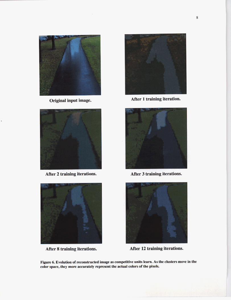
In order to determine when the clustering process should stop (Le. when the cluster weights have converged) a cluster evaluation process must be employed. We have developed a technique which allows the system to perform self evaluation. This technique is based on the ability of the cluster weights to accurately reproduce. or reconstruct, the input image. The self evaluation process begins by classifying every pixel i n the input image according to the most recently updated cluster weights. As in the clustering stage, classification is done locally on each processor on the distributed input image using the previously described closeness measure. Once the closest cluster has been found. the pixel is assigned the red, green, and blue mean values of this cluster contained in the cluster'^ weights. Next, the squared difference between the pixel’s assigned value. given by the closest cluster mean, and its actual value, given by the pixel’s value in the original input image, is computed and stored in local accumulators. After the squared differences have been calculated and stored for a11 pixels on each processor. a global average squared difference table is computed using a global floating point addition operato? and knowledge of the input image size. If the change between the current average squared difference and the previous clustering iteration’s average squared difference for each of the red, green, and blue bands is sufficiently small. clustering ends and the combining algorithm described in the next section begins. If the average squared differences are not yet sufficiently small, the clustering cycle described in the preceding paragraphs repeats using the current cluster weights. The evolution of the reconstructed image as competitive units learn cluster means is shown in Figure 6.

1 . More speciiically, the MasPar MPL reduceAdd320 function is used 2. More specifically, the MasPar MPL reduceAddfO function is used.

7

Figurr 5. As the number of clusters increases, error in reconstruction decreases.

More rigorously, the evaluation process looks at the rate of change, or slope, of average squared difference values. When this slope becomes lower than a user supplied threshold for all three color bands, a minima is said to have been reached, and any further attempts at clustering could yield only minimal improvement. It is important to understand that the rate of change of the average squared difference between actual and reconstructed images is used instead of simply the average squared difference because the rate of change represents the amount of learning that is taking place. If only the average squared difference were used, it would be difficult for the system to know when to stop attempting to cluster, as there would be no way to tell how much learning is taking place. A predetermined lower bound of the average squared difference could be used to terminate learning, but the lower bound value depends upon the number of clusters available to the system. The more clusters that are available to the system, the better the reconstruction that can be done because more clusters in color space can be independently represented. By using the rate of change of the average squared difference, the system can always converge to a locally (in the color space) good solution, regardless of how many clusters are available for i t to use. It has been our e.xperience that approximately 20 cluster-evaluate iterations are necessary for proper clustering of the initial input image.

In the current implementation of our system, the clustering algorithm is run on only the initial image of the color video stream. The correct cluster means may change in subsequent images. Nonetheless, through our experimen- tation on paved roads near campus, we have found that the change is t# small to cause system performance deg- radation. This ditfers from results by [Crisman, 19901 and is potentially due to the greater numbers of pixels

I original input image. After 1 training iteratiom

After 2 training iterations. After 3 training iterations.

After 12 traSning iterations.

Fwrp 6. Evolution of reconstructed image as competitive units leun. As the clusters move in the mbr space, they more acsurateiy represent the actual colors of the pixels.

9

which are used to form the color clusters and the robustness of our combining algorithm. We have not hoked deeply at this difference and it remains open for future study.

4. The Combining Algorithm

In order to determine where the road is located in the input image, it is necessary to separate the road from its sur- roundings. Although it is easy to assume that a single cluster will always classify the road, a.~ the road is almost uniformly gray. and the rest of-the clusters will classify non-road, this is not the case in practice. For example. consider the case of a shadow across the road. In this circumstance, two or more clusters converge to seas in the color space that corresponded to the brightly lit road, the shadowed road, and possibly to the minute color varia- tions in the transition between light and shadow. Since different clusters classify the roadway in this example. a technique must be found to unify this information. No matter if a road pixel is in sunlight or shade, it should he correctly classified as a road. As with the clustering algorithm, the combining algorithm unifies the different clusters of the same type in a distributed manner by using every pixel in the input image. Another feature of this algorithm, similar to the clustering algorithm. is its selfevaluatory nature.

At the h e a t of the combining algorithm is a single, global perceptron with a hyperbolic tangent activation function (See Figure 7.) A perceptron is a connectionist building block used to form artificial neural networks. (See Appendix B for more detail on neural network learning.) This percepwon is trained, by modifying i t s input weights. to differentiate road pixels from non-road pixels using information derived from knowledge of which clusters correctly and incorrectly classify the. pixels in the input image. The output of the perceptron can be thought of as the 'certainty' of a particular pixel having the characteristic color of the road. The perceptron has one input weight for each cluster as well as a bias weight which is always set to 1.0. (Having a bias weight is a standard technique used in perceptron training.) It is important to note that the same global perceptron is used for all pixels on every processor.

Alternatively, a probabilistic methods which take into account cluster size and location could be used to differentiate between road and non-road clusters. This approach has been explored by [Crisman, 19901 and will he discussed in greater detail in section 8.

In order to bootstrap the system, the road region in the initial image is outlined by the user. From this original image, we can determine which colors should be classified as road, and which as non-road. The outline dster- mines the trapezoidal road model. Because we are using a two dimensional mapping. the left and right edges of the outlined region can be superimposed onto the processor array. Processors which lie on these edges are marked, and ones which are hetween the left and right edges are said to contain road pixels while those outside the edges c.ont;rin non-road pixels. This interaction and transformation only occurs once. The algorithm automat- ically proceeds to classify each pixel in the input image using the clusters previously formed. After a pixel has been classified, if i t is located on a road processor (i,e. within the user defined road region), the perceptron is given a target activation value of 1.0. If it is not, the percepunn is given a target activation value of - 1 .0.

The input activation to each connection weight of the perceptron is determined by the following simple rule: if the connection weight is the one associated with the cluster that correctly classified the pixel. it is given an input activation value of 1.0. otherwise it is given an input activation value of -1.0. (See Figure 7. ) Next, each input activation is multiplied by its corresponding connection weight. These products are summed together and this value is passed through the percepmn's activation function which yields its output activation. This process is known as forward propagation. The difference, or error, between the output activation and the target activation is computed. This error, along with the input activation to each connection, is used in the Least Mean Square learning rule IWidrow, 19601, so that each connection's weight adjustment can he computed. These adjustnients are stored in a local accumulator. After all pixels have been processed, the local connection adjustments are summed using the global floating point addition operator and the average adjustment for each connection weight is calculated by dividing the sums by the number of pixels in the image. Each connection weight is then mdified by its computed average adjustment value.

Outputs a value between I (road) and -l(non-road)

-b Trained Weight

.................. Data Flow

.................................

Figure 7. System Architecture. Every input pixel is classified in parallel by competitive learning units (CL #I-N). The winning unit, determined by the Winner-Take-All (WTA) units, has its output activation set to 1 while all others are set to -1. Again in parallel, a perceptmn classifies this combination of inputs as either mad or non-road.

As with the clustering algorithm, a method has been developed which allows the system to detemine when learning should be stoppad. Using this method, the output activation of the perceptron along with the difference between the target and actual output activation is calculated and stored, as before. for every pixel in the input image. After all pixels have been processed, the avenge pixel errur is computed and compared to the average error kom the previous perceptron training iteration. Ifthis difference is sufficiently small, learning is halted. If it is not, another iteration of perceptron training is commenced using the new percepbon connection weights (See Figure 8.) The reasons for using this method of self evaluation are similar to those for the clustering algorithm: in this case we are measuring the rate of learning of the perceptron instead of the clusters. After perceptron training is completed, when pixels which are part of the road are shown to the system they will be classified uniformly as road, regardless of which individual cluster correctly classified them. In our case, the output of the perueptron for a road pixel is near 1.0 while the output for a non-road pixel is close to -1.0.

After 1 training iteration. After 2 training iterations.

After 3 training iterations.




Figure 8. As the perceptron learns, its output better classifies road and non-road. The white pixels represent on-md, while the black off-road.

5. The Road Finding Algorithm

In order for the system to successfully navigate the vehicle, it must find the correct path to follow. We will assume that a safe path is down the middle of the road. (By finding the center line of the road, offsets can be computed to drive on the left or right sides as needed Because our test path is a paved, three meter wide bicycle path, simply finding the center line is sufficient.) The technique that our system employs is a parallelized version of3 Hough transform. (See Appendix C for an introduction to Hough transforms.) Hough transforms and related techniques are not new to the field of Parallel Computing. but because our work crosses traditional boundaries, (those between Parallel Computing, Neural Network, and Robot Navigation) a detailed description of our algorithm. and how it relates to the domain of autonomous roadway navigation, is warranted. We use the topology of the processor m a y to simulate the parameters of the Hough space and determine the location of the center line of the road by searching for the most likely combination of all possible parameters. The parameters which we m trying to find are the intersection column of the center line and the top row of the image and the angle of the center line with respect to the top row.

The first step of the road finding algorithm is to assign each processor in the array a probability of being road. This is done by averaging the perceptron output activation values of all pixels within a particular processor, as defined by the two dimensional hierarchical mapping scheme. and scaling them to a value between 0 and 255. Because the output of the perceptron can be thought of as the ‘certainty’ of a pixel belonging to the road. the average percepmn output for a processor is related to how many road pixels the processor contains. A higher average value indicates more road pixels while a lower value indicates the processor contains many non-road pixels. Processors which lie on road edges ace expected to have intermediate values while ones within the edges areexpected to have high average values. In this formulation. 0 represents non-road and 255 represents road. See Appendix D for details about alternative pixel averaging techniques.

Because the mad edges were marked in the combining algorithm and because we use a two dimensional hierarchical mapping, it i s easy to compute how wide, in terms of processors, the mad is at each row in the processor array. (See Figure 9.) We will assume that the width of the physical road is constant and that perspective effects cause the same amount of foreshoItening in all images that the system evaluates. Empirically, this has proven to be a reasonable assumption. Moreprecisely, once we determine that the road is 4 processors wide in the first row. 6 processors wide i n the second, 9 in the third, etc.. these road width values for each row are held constant for all future images. Because the camera lookahead is kept small, this is a reasonable assumption. If the camera lookahead was large, problems would arise in the case of sharp curves and hills in the road; the fi~d width assumption of each row defined by the trapezoidal road model would no longer be valid.

The next step is to center a contiguous, horizontal, summation convolution kernel on every processor in the array. (A summation convolution is defined as one in which all values marked by the kernel are added together. The kernel specifies how many processors are to be included in the summation.) The width of this convolution kernel is given by the road width for the NW in which the processor is located as determined in the previous paragraphs. The convolution kernel is implemented using local, synchronized, neighbor-to-neighbor communications functions’ and is therefore computed very quickly. Because the convolution kernel is larger for rows lower in the pm- cessor array, not all processors shift their data at the same time. This slight load imbalance is insignificant. By using this summation convolution kernel, we have essentially computed the likelihood that the road center line passes through each processor. Processors which are near the actual road center line have larger convolution values than ones which are offset from the actual center because the convolution kernel does not extend onto non- road processors. The convolution kernel for processors which are offset from the actual road center will include processors which have low probability of being road because the underlying pixels have been classified as non- road, The convolution process is shown in Figure 9.

3. More specifically, the MasPar MPL met0 functions are used.

13

7 7 8 9 10 10 10 12 12 14 14 15 15 16 17 17 19 19 19 20 ~. 21 22 22 24

Convolution kernel widths for each row of the processor array. The widths are determined at stan-up from the initial image of the road.

Figure 9. Convolution kernels for different mws centered on the actual center line of the road superimposed on the processor array. Arrows indicate the direction of travel of ihe convolution summation.

Finding the road's center line can be thought of as finding the line through the processor array which passes through processors which contain the largest aggregate center line likelihoods. This is equivalent to finding the maximum accumulator value in a classical Hough transform where the intersection row and intersection angle are the axes of the Hough accumulator. To parallelize this Hough transform, we can shift certain rows of the processor array i n a predetermined manner and then sum vertically up each column of the array. The shifting gives us the different intersection angles and finding the maximum vertical summation allows us to determine the intersection of the center line with the top mw of the image. Before the first shift takes place, a vertical summation of the center line likelihoods up the columns of the processor array is done. In this preshifted configuration, the inaximum column summation value will specify the most likely vertical center line. The column in which the maximum value is found will determine the intersection of the center line with the top row of the input image. Similar statements hold for all shifts and summations.

The shifting pattern is designed so that after the first shift, the row centerline likelihood in the bottom half of the processur array will be one column to the east from its original position. After the second shift, the bottom third will he two columns to the east. the middle third will be one column to the east and the top third will still have not moved. This pattern can continue until the value of the middle processor in the bottom row has been shifted to the east edge of the processor may. This will happen after 32 shifts in either direction. In practice. this many shifts is not required as the extreme ones do not occur in typical road images. (See Figure 10.) Shifting to the west is done concurrently in a similar manner. This shifting represent examining the different center line intersection angles in the Hough accumulator. Because of the way the values are shifted, vertical binary addition up the columns of the processor array can be used to compute the center line intersection and angle parameters. [ In this context, binary addition does not refer to binary number addition, but rather to summing using a binary tree of processors.) By finding the maximum vertical summation across all east and west shifts. the precise intersection and angle can be found very efficiently. (See Figure I1 .) Once the intersection column and angle of the center line have been found, the geometric center line of the road can be computed.This geometric description of the center line is passed to the vehicle controller for transformation into the global reference frame and is used to guide the vehicle. This algorithm, while perhaps the hardest to understand, most elegantly makes use of thr tightly coupled processor array. One note about this algorithm: it does not take into account the orientation of the camera when computing the shift parameters. It assumes that the camera i s aligned with the mad in all anis except for pitch (up and down). If the camera is in any orientation other than this, the shifted image will not accu-

14

0 Shifts 1 Shifts 2 Shifts

3 Shifb 4 Shifts 5 S h i h

Figure 10. Original center line data after 0 through 5 shilts X’s in processors represent non- valid data. The shading represents different columns and does not signify any mad features.

Potential center lines in unshifted array. Potential center lines in shifted array.

Figuro 11. After shifting, center lines which were originally angled, are aligned vertically. Summation up the columns of the processor array can then determine the most likely intersection angle and column.

15

rately resemble the actual road. In reality the canieril is not aligned in this manner, but the deviation is small enough that i t does not d e p d e system pe~ormance .

6. Runtime Processing

Once all clusters and the perceptron have been trained, the system is ready for use either in simulation or physical control of our vehicle. Jnput images are received by the processor m a y and pixel classification occurs using the precomputed cluster means. The perceptron uses this classification to determine if the pixel is part of the road. The perceptron’s output is supplied to the road finding algorithm which determines the center line location. The center line location is transformed onto the ground plane and is passed to the vehicle controller wrhich guides the vehicle. At this point, learning is complete and the iterative form of the clustering and combining algorithms are no longer necessary.

7. Results

The results obtained, both in simulation and driving the vehicle, were very encouraging. The simulation results i n terms of color frames processed per second are summarized in Table 1. These results represent average actual processing speed, in terms of frames processed per second, measured when running our system on the specified machine with the set image size.. As the number of pixels increased, the frames processed per second decreased in a roughly linear fashion. The slight irregularity is due to the convolution kernel in the road finding algorithm. It is also interesting to note that the 16K MasPars did significantly worse than the 4K machines as the image size decreased Again, this is due to the convolution kernel in the road finding algorithm. We believe that this is not a load imbalance problem but rather a side effect of having a physically larger array topology. Because of the extra width of the processor array, more local neighbor-to-neighbor communication operations are required to compute the summation convolution. As the image size was decreased, these operations came to dominate the processing time.

We are very pleased with the fact thatframe m e complrlotion was achieved on a 4K MasPar MP- 1 machine for the 256x256 pixel image case and on a 16K MasPar MP-2 for the 512x512 pixel image case. Although our ulti- mate goal is to develop algorithms which can process 5 12x512 color image streams at frame rate on our 4K Mas- Par MP-I, we are excited about the results of our initial experiments. Clearly. fine-grained SIMD machines provide a significant benefit in real world vision tasks such as autonomous navigation. On test runs of our tesL-

Table 1. System performance in color frames processed per second.

bed vehicle. the Navlab I, the system has been able to successfully navigate the vehicle on a paved bike path using 128x128 images. At present, the major bottleneck is the slow digitization and communication hardware

16

which is supplying the MasPat with images. This bottleneck limits the image size to 128x128 and Lhe cycle time to approximately 2.5 Hz. Even so. the system has consistently driven the vehicle in a robust manner over the entire 600 meter path. For comparison, other systems that have been developed are ALVINN. which processes 30x32 images at 1U Hz (4 times slower) and SCARF, which processed 60x64 images on a 10 cell Warp super- computer at 1/3 Hz (32 times slower). [Cnsman 1990][Crisman, 199 11 These figures include image digitization time and slow-downs are computed based on pixels prncessed per second.

A better comparison of processing speed may actually be the time processing the image, not including image acquisition. As an example of this, consider the SCARF system which was also implemented on a parallel machine. For the this system running on the W.arp machine, a 60x64 images could be processed in one second. [Crisman, 19911 Comparing this to our system (running on a 4K MF-I) processing 64x64 images at h9.4 Hz yields a 74 times speed improvement. For a 1024x1024 image, a 846 times speedup is achievable. On 3 16K MP- 2, for 128x128 images, processing is 158 times faster and for the 1024x1024 case on this machine, a speedup of over SO00 can be realized. Again, slow-downs are computed based on pixels processed per second. Results of this order were expected as we designed algorithms for the fine-grained parallel machines on which they ran.

The trade-iff between the number of clusters the system employs and the frame rate is shown in Figure 12. We can see how the frame rate decreases with an increase in the number of clusters for three different size images. Because we are interested in achieving frame rate cycling speed, and due to the minimal driving performance improvement achieved by using more clusters, it was determined that 5 clusters were sufficient for our needs.

Clusters

Figure 12. As the number olelusters increases, it hecomes much harder to achieve frame-rate computation.

17

Finally. the performance figures quoted in the table do not include image acquisition time. At present, using a VME based digitizer, image acquisition consumes a significant amount of time and limits our driving speed to about 10 m.p.h. Although our system is capable of driving at much faster speeds, it is disappointing that actual driving results are limited by supporting hardware deficiencies. This problem once again underscores the need for high performance YO devices to supply parallel machines with data. To remedy this problem, a 512x512 pixel color frame-rate digitiser and interface i s being built for our 4K MasPar MP-I. This hardware will deliver images to the processor array with very low latency and d low us to run the system at rates predicted i n the simulation results and drive the vehicle at much faster speeds.

8. Other Related Systems

Our system compares very well against any road following system in use today in terms of processing speed. Three competitive high performance systems are the ALVI" and MANIAC systems [Pomerlem, 1992][Jochem, 19931, developed at Carnegie Mellon University, and the system designed by the VaMoRs group in Munich, Germany. Like ours. the ALVI" and MANIAC systems are neurally b a d . Huwever. both use reduced resolution (30x32) preprocessed color images. They cycles at about 10 frames per second, using SPARC based pracessors. and ALVINN has driven for over 22 miles at speeds of up to 55mph (88 kmhr). A system which is founded i n very different techniques is the one being devcloped by the VaMoRs group [Dickmanns. 19921. This system, which uses strong road and vehicle models to predict where road features will appear i n upoming images. processes monochrome images on custom hardware at speeds ne= frame rate, but u x s a windowing system to track the features so that not every pixel is actually processed. This system has been able to successfully drive on the German Autobahn at speeds around 8 0 W r .

Various other systems have been developed that use color data and include the VITS system developed at Martin Marietta [Turk, 19881 and SCARF developed by [Crisman, 19901 at Carnegie Mellon University. The VITS system used a linear combination of the red and blue color hands to segment the road from non-road. The segmented image was thresholded and backprojected onto the ground plane. The vehicle was steered toward the center of this backprojected region. This system was able to drive Martin Marietta's testbed vehicle, the ALV, at speeds up to ZOkm/hr on straight, single lane roads found at the test site.

Perhaps most closely related to our system is SCARF Like our system, SC;\RF uses color images to develop clusters in culor space. These images are greatly reduced; typically 30x32 or 60x64 pixels. The techniques for developing these clusters, however, is very different from the one implemented in our system. SCARF uses Bayesian probability theory and a Gaussian distribution assumption to create and use color clusters to segment incoming color images. The clusters are recreated for every input image by using a strung road model and known road and non-road data as seed points for the new cluster means. The computational load of SCARF is higher than that of our system because of the Bayesian and Gaussian computations and, partially because of this load. the system was only able to drive at speeds of less than 10 m.p.h. The most closely related part of our system and SCARF is the Hough transform based road finding algorithm. Because the Hough algorithm maps very well to finding single lane roads, it was adapted to the parallel framework of our system. Although the implementation of the Hough algorithm is different, the concept remains the same. Finally. it should be noted that the SCARF system did many other things that our system does not do, like intersection detection and per-image updating of the color cluster means. SCARF needed to be smarter because it took a significant amount of time to process a single image.

9. Future Work

We feel that the most limiting aspect of the current system is the model used to determine the center line of the road Because the model defines the road to be a trapezoidal region which is bisected by the center line, errors i n driving can occur when the actual road does not match this model. A commonly occurring situation when the mad difFers from the model is during sharp curves. The best trapezoidal region is fit to the data and a center line is found. Unfortunately, when this center line is driven, i t causes the vehicle to "cut the corner." Although the system will quic.kly recover. this is not desirable behavior. We believe that by using a different road model this

18

problem can be solved. We propose to use a road model based on the turn radius of the road ahead. By using this model, roads with arbitrarily curvature can be properly represented. Instead of driving dong a straight line pro- jected onto the ground plane, the vehicle will follow the arc determined by the most likely turn radius. This model can be implemented as a parallelized Hough transform in much the same way as the current trapezoidal model. The only difference will be the shift amounts of each row of the processor array at each time step. By using this model, we feel better driving performance can be obtained without sacrificing computational speed.

Another area of future research is the effect of changing lighting conditions on the performance of our algorithms. We assume the first image our system processes will contain a representative sample of all color varia- tions which will be seen during navigation. Because of this assumption we are susceptible to errors caused by severe changes in lighting conditions that appear in later images. If the clusters which are learned during the competitive learning training process cannot adequately classify later images, the perceptron which combines all the clusters' output into a road or non-road classification. may receive incorrect information which will lead to misclassification. Although we have found that this effect can be ignored going from sunlight to fairly heavy shade, it is important to realize that the lighting condition is not the only parameter which controls a cluster's ability to correctly classifi data. Another important parmeter is the. number of clusters which are available to the system. If many clusters are available, finer discrimination is possible. Essentially this means that the color space is better covered by the clusters. In a statistical sense, when many clusters are available, the covariance of any particular cluster will be less than that of a cluster belonging to a smaller cluster set. Intuitively, a smaller covariance implies that the mean value of a cluster (or any data set) better represents all the data which is classified as being part of that data set. So if many clusters are available, it is reasonable to assume that a wider range of lighting conditions can be tolerated because it is more likely that some of the clusters developed in the original learning process are specific to more areas in the color space relative to clusters developsd when few are available. Our results do support the notion that better coverage is possible when more clusters are available (See Figure S.), but a more interesting idea that can be explored is that of dynamically adding, removing. or adapting clusters as lighting conditions change. Of course, the addition of clusters must be traded with computation speed, but, perhaps more imponantly, this type of algorithm would allow new clusters to be developed when current clusters do not adequately classify the scene. When new clusters arise in color space, or current ones simply shift, new clusters could be formed which better represent the new color space. The SCARF system used a similar technique, but instead of adding. removing, or adapting clusters when needed, new clusters were created for every image using a predictive model of the road as aid to classification. A system incorporating an adaptive cluster management algorithm could likely handle extreme shifts in lighting conditions and robustly drive in a wider range of operating scenarios.

Finally, we feel that it may be possible to completely eliminate the color clusters from our system. Because the road and non-road clusters in color space form two nearly disjoint sets, a plane could be used to discriminate between mad and non-road pixels. To learn this plane, the perceptron, or possibly a small neural network. would take as input the red, green, and blue values of a pixel and learn to produce at its output a 1 if the pixel is part of the road and a - I if it is not. In theory, a perceptton with a thresholding activation function could accomplish this task. but because the road and non-road sets come very close to each other in the low intensity regions of the color space, a neural network may be needed for proper discrimination.

10. Conclusions

Our system has shown that fine-grained SLMD machines can be effectively and efficiently used in real world vision tasks to achieve robust performance. By designing algorithms for specific parallel architectures, the resulting system can achieve higher performance than if the algorithms were simply ported to the parallel machine from a serial implementation. The system described in this paper uses substantially larger frames and processes them at faster rates than other color mad following systems. The algorithms presented here were tested on 4K and 16K processor MasPar MP-1 and on 4K. 8K, and 16K processor MasPar MP-2 parallel machines and were used to drive Camegie Mellon's testbed vehicle, the Navlab I, on paved roads near campus.The goal that our work has strived toward is processing 512x51 2 pixel color images at frame rate in an autonomous road following system. Our results have shown that in this domain, with the appropriate mapping of algorithm to architecture,

19

frame rate processing is achievable. Most importantly, our results work in the. real world and not simply in simulation.

11. Acknowledgments

We would like to thank Dr. Edward Delp and his staff in the Parallel Processing Lab at Purdue University for allowing us access to their 16K MasPar. Their machine was purchased in part though NSF award number CDA- 9015696. Performance tests on the MP-2’s were conducted for us by Philip Ho of MasPar Computer. We greatly appreciate his help. Also, we would like to thank Bill Ross, Jim Moody and Dean Pomerleau for their help in installing our new 4K MP-1 on the Navlab 1. Thanks are also due to Bill Ross, Chuck Thorpe, Jon Webb, Jill Crisman, and Dean Pomerleau who served as editors for this report Their varied perspectives helped unify the navigation: parallel computing and connectionist ideas.

Appendix A: Competitive Learning

Competitive learning is an unsupervised connectionist learning technique which attempts to classify unlabeled training data into significant clusters or classes in some features space. In this framework. many units compete to become active, or turn on. when presented with input training data The single unit which wins is allowed to learn Because this techniques is unsupervised, i t q u i r e s no teaching signal to tell the units what to learn. The units finds relevant features based on the correlation present in the unlabeled training data.

A typical competitive learning network is composed of several output units 0, which are fully connected to each input through a connection weight. To find the activation of the unit, the input activations, cj, are multiplied by the corresponding connection weights, wjj,and summed to produce an output activation. See equation (1).

The output unit which has the largest activation is declared the winner. If weights for each unit are normalized, then the winning unit, denoted with by is, can be defined as the unit whose inputs most closely match its input weights. This can he expresses as:

Because the weights in each unit staIt out as random values, a method is need to train them. The intuitive idea is to learn weights which will allow the unit to correctly classify some portion of the feature space. The method that is typically used, and the one used in this system, is to move the weights of the winning unit directly towards the input pattern. This technique is know a% the standard competitive learning rule. Mathematically speaking. this rule can be expressed as

k = O

where u represents the training pattern number and q. An important thing to notice about equation (3) is that the contribution of each training pattern to the overall weight change can be computed independently. This means that this contribution can becalculated concurrently for many training patterns at once. It i s this type of algorithm which can take advantage of a fine-grained parallel machine and is a major reason why it was chosen.

20

Appendix adapted from [Hertz, 1991 1

Appendix B: Artificial Neural Networks

An Artificial Neural Network (ANN) is composed of many small computing units. Each of these uniLs i5 looscly based upon the design of a single biological neuron. The key features of each of these simulated neurons are the inputs. the activation function. and the outputs. A model of a simple neuron is shown in Figure 13. The inputs to

inputs weighted connections

output

N

- t

i = 0

activation function

Figure 13. The arti icial neuron works as follows: the summation of the incoming (weights * activation) values is put through the activation function in the neuron. In the above shown case, this is a sigmoid. The output of the neuron, which can be fed to other neurons, is the value returned from the activation function. The x’s can either be other neurons o r inputs from the outside world.

each neuron are multiplied by connection weights giving a net total input. This net input is passed through a non- linear activation function, typically the sigmoid or hyperbolic tangent function, which maps the infinitely ranging (in theory) ne t input to a value between certain limits. For the sigmoidal activation function, input values will be mapped to a point in (0, I ) and for the hyperbolic tangent activation function, the input will be mapped to a value in (-1,l). We have chosen to use the hyperbolic tangent activation fuoction because in practice the symmetry of this function allows an inactive unit (with -1 activation) to contribute to the net input of units to which it has connections. This mapping is also know as ‘squashing‘ and allows the network to internally represent a wide range of inputs with a small set of values. ‘Squashing’ contributes to the network’s ability to generalize. Once the ‘squashed’ value has been computed, it can either be interpreted as the output of the network, or used as input to another neuron.

Artificial neural networks are generally composed of many the units show above, as shown in Figure 14. For a neuron to return a particular response for a given set of inputs, the weights of the connections can be modified. Training” a neural network refers to modifying the weights of the connections to produce the output vectur associated with each input vector.

A simple ANN is composed of three layers, the input layer, the hidden layer and the output layer. Between the layers of units are connections containing weights. These weights serve to propagate signals through the network. (See Figure 14.) Given any set of inputs and outputs, and a sufficiently large. network, a set of connection weights exists which can correctly map the network’s input to the desired output. The process of finding a correct weights is known as “training the network.” Typically, the network is trained using a technique which can be thought of as gradient descent in the connection weight space. Once the network has been trained, given any set of inputs which are similar to those on which it was trained, it will be able to reproduce associated outputs by propagating the input signal forward through each connection until the output layer is reached.

21

Weighted Connections Inputs

Input Layer Hidden Layer Output Layer

Figure 14. Shown is a fully connected three layer ANN. Each o l t h e connections can change i ts weight independently.

In order to find the weights which produce correct outputs for given inputs. the most commonly used method for weight modification is error backpropagation. Back-propagation is simply explained in Abu-Mostafa's [Abu- Mostafa. 19891 paper "Information Theory, Complexity and Neural Networks":

... the algorithm [backpropagation] operates on a network with a fixed architecture by changing the weights, in small amounts. each time an exampleyi =flx,J [where y is the desired output pattern. and x is the input pattern] i s received. The changes are made to make the response of the network to xi closer to the desired output, yi. This is done by gradient decent, and each iteration is simply an error signal propagating backwards in the network in a way similar to the input that propagates forward to the output. This fortunate property simplifies the computation significantly. However, the algorithm suffers from the typical problems of gradient descent, it is often slow, and gets stuck in local minima.

Artificial neural networks were chosen as the learning tool because of their ability to generalize. If ANN'S we not overtrained and are sufficiently large, after training, they should be able to generalize to input patterns which have not yet been encountered. Although the output may not be exactly what is desired, it should not be a cata- strophic failure either, as would be the case with many non-learning techniques. Therefore, in training the ANN, it is important to get a diverse sample p u p which gives a good representation of the input data which might be seen by the network during simulation.

Appendix Adapted from maluja, 19931

Appendix C: Hough Transform

The Hough Transform was first developed as a technique for finding curves in the plane (or in space) when little is known about the curve's spatial location. Every point which is potentially a member of the curve is considered. (A common way of finding potential points is through the use of an edge detection algorilhm.) Once a point has been found. all possible parameter sets of curves passing through the point are determined. For example, the parameter set for a line in Cartesian space is (m, b). For a circle it could be (x. y, r) where x and y are the location of the center of the circle and r is the circle's radius. After a possible parameter set has been determined, a location in an accumulator which corresponds to the set is incremented. Once all potential points have been considered, the accumulator is searched for a maxima. The maxima will give the parameter set for the most likely curve.

The classic example describing the Hough Transform deals with finding lines in images. In this example, you are given Ihe location of all possible edge points. The task is to find the lines to which these edge points belong, The

general idea is to map point.; in (x. y) space to locations i n a (m. b) space accumulator where (m. b) are determined by-

Y = m X + b (4)

This equation is simply that of a line in the plane. For every (x. y) edge point, all possible (m. b) points are coni- puted. The (m, b) location i n the accumulator is incremented. In the accumulator. the (m, b) points that are found for a particular. fixed, (x. y) are also a line in the accumulator that is described by:

Graphically, these equations look as follows.

The equation of this line has slope m l and y intercept bl .

b= 411x2 + y2

(ml. b l )

. . Figure IS. Transformation from Cartesian space to Hwgh Space. [Ballard, 19821

Appendix D: Alternative Pixel Averaging

An alternative method of finding one average ‘certainty’ value of the pixels in each processor is to average the red. green, and blue pixel values respectively across each pixel represent4 in the processor. This could be done when the image is first mapped onto the processor array. The average pixel value could then be fed to the competitive. learning u n i t s which would determine the closest matching cluster, and finally to the perceptron which would create a road or non-road output ‘certainty.’ Extending this analysis, there are 2 alternatives to the method of learning which can be used, with 2 corresponding alternatives for simulation of the network. (Se.e Figure 16.) Each of the combinations represents trade-offs between speed and accuracy of color clusters versus actual image. colors.

23

LEARNING

Avg. RGB Values

Training is on average pixel values. Simulation is on average pixel values.

The colors used for training and simulation may not exist in the image.

Requires the least processing time.

Only outputs 0 or I for each pixel group

Training is on average pixel values. Simulation is on actual pixel values

The pixel values used for simulation may not be consistent with learned clusters.

Outputs are a real number for each pixel group.

Avg. Perceptron Values

Training is on actual pixel values. Simulation is on average. pixel values.

The pixel values used for simulation may not be consistent with learned clusters.

Only outputs 0 or 1 for each pixel group.

Raining is on actual pixel values Simulation is on actual pixel values.

The colors used for training and simu. lation do actually exist i n the image.

Requires the most processing time.

3utputs are a real number for each ixe l group.

Figure 16. Figure compares where averagingis performed. “Avg. RGB ValuePindicates that pixel values are averaged before being presented to the system, effectively being preprocessed, reducing the amount of data. “Avg. Perceptron Values” indicates that averaging i.i done after each pixel has been propagated through the system and has produced a ‘certainty’ value. The ‘Learning’ axis indicates which process takes place during the training phase of the system. The ‘Simulation’ axis indicate which p m w takes place after the clustering and combining algorithms have learned. Our system uses the configuration shown in the bottom right corner.

Appendix E: The MasPar MI’-1

The hardware used to perform the test runs was the MasPar Mp-1. This is a massively parallel computer, consisting of an Array Control Unit (ACU) and a two dimensional array of processing elements (PES). The array size is 64 x 64, for a total of 4096 processing elements. The ACU has 1 Mbyte of RAM with up to 4 Gbyte of virtual instruction memory. The ACU is used to conbal the PE array and to perform instruction on data which is not located on the PE’s dedicated memory. Each PE has 16 Kilobytes of dedicated RAM. The MasPar is a Single Instruction Multiple Data (SIMD) machine. Put simply, this means that each PE receives the same instruction simultaneously from the ACU. Through control statements, processors can be either active or non-active. The P E S which are members of the active set will execute the instruction they receive from the ACU. on Iocul datu. Those which are not members of the active set will do nothing [Maspar. 19921.

The processors can be accessed either through relative addressing mode (from other processors) or absolute addressing. Further, they have two modes of numbering for identification. They can either be accessed by x,y coordinates or by row-major ordering. This allows an efficient programminp model for the three implementa- tions described in the next section.

24

The programming language used was the MasPar Parallel Application Language (MPL). This is an extended set of Kernighan and Ritchie C with extra directives for controlling the PE array and parallel data structures. The images were generated with the h4asP‘u XMPDDL library.

Appendix from [Baluja. 19931

Appendix F: MasPar Programming Language

The following function definitions are more precisely specified i n [Maypar. 19921 and are provided here in acon- densed form tor your convenience.

reduceAdd32 (integer-variable) - This functions takes a distributed integer variable as input and returns the integer sum of it across all (active) processor elements.

reduceAddf (SPJTnuting point variable) - This functions takes a distributed single precision floating point variable as input and returns the single precision floating point sum of i t across all (active) processor elements.

xnet{N,S,E,W,NE,NW,SE,SW}[num].variable - The xnet construct allows active processor elements lo communicate with other processor elements which are a fixed distance, num, away in the specified direction. The variable argument in the constmct determines which variable is communicated.

References IAbu-Mostafa, 19891 Abu-Mostafa. Y. “Information Theory, Complexity, and Neural Networks”’, IEEE Corn-

municafions Magazine. V01.27, No. 11, 1989.

[Ball. 19671

[Ballanl. 19821

[Baluja, 19931

[Cnsman, 19901

[Crisman, 19911

[Dickmanns, 19921

[Hertz, 19911

[Jochem, 19931

[Kluge, 19921

Ball. G . H. and Hall, D. J.. “A Clustering Technique for Summarizing Multivariate Data,” Behavioral Science, Vol. 12, pp. 153-155. M m h 1967.

Ballard, D. H. and Brown, C. M. “Computer Vision,”Prentice-Hall. 1982. pp. 123-124.

Baluja, S., Pomerleau, D.A., and Jochem. T.M. ’“Towards Automated Artificial Evolution for Computer Generated Images,” paper i n progress.

Crisman, J. D. ‘Color Vision for the Detection of Unstructured Roads and Intersections,‘’ Ph.D. Thesis, Electrical and Computer Engineering Depamnent, Carnegie Mellon Univer- sity, Pittsburgh, PA, USA, May, 1990.

Crisman. J. D. and Webb, J. ‘The Warp Machine on Navlah.” lEEE Transactions on Pat- rem Analysis and Machine Intelligence, Vol. 13, No. 5. pp. 451465, May 1991

Dickmanns, E. D. and Mysliwetz, B.D. “Recursive 3-D Road and Relative Ego-State Rec- ognition.” IEEE Transactions on Pasern Analysis and Machine Intelligence, Vol. 14. pp. 199-213, May 1992.

Hertz, J., Krogh, A.. and Palmer, R.G. “Introduction to the Theory of Neural Computa- tion,” Addison-Wesley, 1991. pp. 217-221.

Jochem. T.M., Pomerleau. D.A., Thorpe, C.E. “MANIAC: A Next Generation Neurally Based Autonomous Road Follower,” In Proceedings of ZAS-3, Feb. 1993, Pittsburgh, PA. USA.

Kluge, K. and Thorpe, C.E. “Representation and Recovery of Road Geometry in YARF.” In Proceedings of the Intelligent Vehicles ‘92 Symposium June. 1992.

25

(MasPar, I9921 MasPar Programming Language Reference Manual, Software Version 3.0, July, 1992, MasPar Computer Corporation.

Pomerleau, D.A. "Efficient Training of Artificial Neural Networks for Autonoinous Navi- gation," Neural Computation 3: I , Terrence Sejnowski (Ed).

Thorpe, C.E., editor, "Vision and Navigation: The Carnegie Mellon Navlab." Kluwer Aca- demic Publishers.

Turk, M. A,, Morgenthaler, D. G.. Gremban, K. D.. and Marra, M. "VITS - A Vision Sys- tern for Autonomous Land Vehicle Navigation," IEEE Transactions on Pattern Analyis UndMachineInlelligence, Vol. 10, No. 3, May 1988.

Widrow. B. and Hoff. M.E. "Adaptive Circuit Switching." In IY60 IRE WESCON Conven- tion Record, part 4, pp. 96-104. New York: IRE.

[Pomerleau. I99 1 ]

[Thorpe, I9901

[Turk, 19881

[Widrow. 19601

Massively Parallel, Adaptive, Color Image Processing for

Documents

Transcript of Massively Parallel, Adaptive, Color Image Processing for