Massachusetts Institute of TechnologyDepartment of Electrical Engineering and Computer Science

6.685 Electric Machinery

Class Notes 8: Analytic Design Evaluation of Induction Machines

©c 2005 James L. Kirtley Jr.

1 Introduction

Induction machines are perhaps the most widely used of all electric motors. They are generallysimple to build and rugged, offer reasonable asynchronous performance: a manageable torque-speedcurve, stable operation under load, and generally satisfactory efficiency. Because they are so widelyused, they are worth understanding.

In addition to their current economic importance, induction motors and generators may findapplication in some new applications with designs that are not similar to motors currently incommerce. An example is very high speed motors for gas compressors, perhaps with squirrel cagerotors, perhaps with solid iron (or perhaps with both).

Because it is possible that future, high performance induction machines will be required tohave characteristics different from those of existing machines, it is necessary to understand themfrom first principles, and that is the objective of this document. It starts with a circuit theoreticalview of the induction machine. This analysis is strictly appropriate only for wound-rotor machines,but leads to an understanding of more complex machines. This model will be used to explain thebasic operation of induction machines. Then we will derive a model for squirrel-cage machines.Finally, we will show how models for solid rotor and mixed solid rotor/squirrel cage machines canbe constructed.

The view that we will take in this document is relentlessly classical. All of the elements thatwe will use are calculated from first principles, and we do not resort to numerical analysis orempirical methods unless we have no choice. While this may seem to be seriously limiting, it servesour basic objective here, which is to achieve an understanding of how these machines work. It isour feeling that once that understanding exists, it will be possible to employ more sophisticatedmethods of analysis to get more accurate results for those elements of the machines which do notlend themselves to simple analysis.

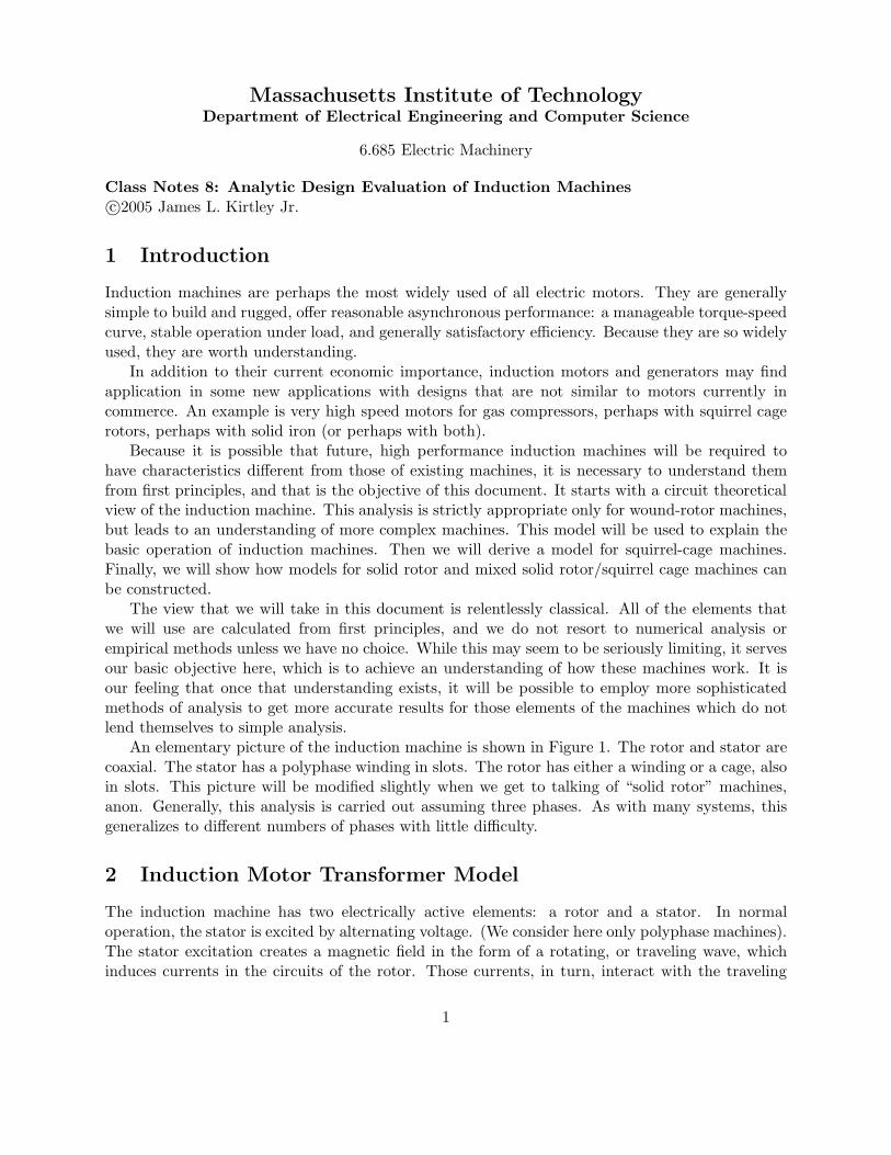
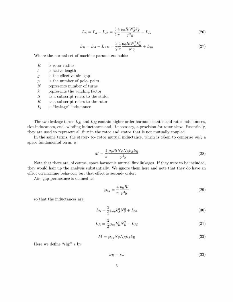
An elementary picture of the induction machine is shown in Figure 1. The rotor and stator arecoaxial. The stator has a polyphase winding in slots. The rotor has either a winding or a cage, alsoin slots. This picture will be modified slightly when we get to talking of “solid rotor” machines,anon. Generally, this analysis is carried out assuming three phases. As with many systems, thisgeneralizes to different numbers of phases with little difficulty.

2 Induction Motor Transformer Model

The induction machine has two electrically active elements: a rotor and a stator. In normaloperation, the stator is excited by alternating voltage. (We consider here only polyphase machines).The stator excitation creates a magnetic field in the form of a rotating, or traveling wave, whichinduces currents in the circuits of the rotor. Those currents, in turn, interact with the traveling

1

Stator Core Stator Windingin Slots

Rotor Windingor Cage inSlots

Rotor

Air−Gap

Figure 1: Axial View of an Induction Machine

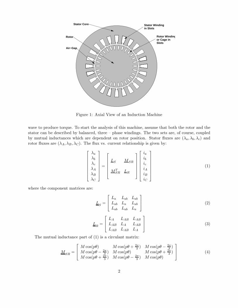
wave to produce torque. To start the analysis of this machine, assume that both the rotor and thestator can be described by balanced, three – phase windings. The two sets are, of course, coupledby mutual inductances which are dependent on rotor position. Stator fluxes are (λa, λb, λc) androtor fluxes are (λA, λB , λC). The flux vs. current relationship is given by:

λa

λb

LS

ia

i

b

Mλ

Rc

S

i=

λA

λB

MTSR LR

c (1)

iA

iB

λ i

C C

where the component matrices are:

LL =

a Lab Lab

L L ab a LabS

Lab Lab La

(2)

LA LAB LAB

L = LAB LA LABR

LAB LAB LA

(3)

The mutual inductance part of (1) is

a circulant matrix:

M cos(pθ) M cos(pθ + 2π ) M cos(pθ3 − 2π )3M =

M cos(pθ − 2π ) M cos(pθ) M cos(pθ + 2π )SR

3 3

(4)M cos(pθ + 2π ) M cos(pθ3 − 2π ) M cos(pθ)3

2

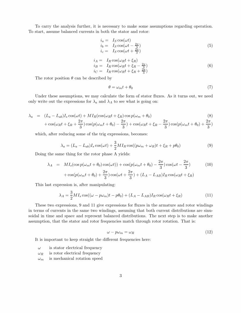
To carry the analysis further, it is necessary to make some assumptions regarding operation.To start, assume balanced currents in both the stator and rotor:

ia = IS cos(ωt)ib = IS cos(ωt− 2π ) (5)3ic = IS cos(ωt+ 2π )3

iA = IR cos(ωRt+ ξR)i = I cos(ω t+ ξ − 2πB R R R ) (6)3iC = IR cos(ωRt+ ξ + 2π

R )3

The rotor position θ can be described by

θ = ωmt+ θ0 (7)

Under these assumptions, we may calculate the form of stator fluxes. As it turns out, we needonly write out the expressions for λa and λA to see what is going on:

λa = (La − Lab)Is cos(ωt) +MIR(cos(ωRt+ ξR) cos p(ωm + θ0) (8)

2π 2π 2π 2π+ cos(ωRt+ ξR + ) cos(p(ωmt+ θ0) − ) + cos(ωRt+ ξR − ) cos(p(ωmt+ θ0) + )

3 3 3 3

which, after reducing some of the trig expressions, becomes:

3λa = (La − Lab)Is cos(ωt) + MIR cos((pωm + ωR)t+ ξR + pθ0) (9)

2

Doing the same thing for the rotor phase A yields:

2π 2πλA = MIs(cos p(ωmt+ θ0) cos(ωt)) + cos(p(ωmt+ θ0) − ) cos(ωt

3− ) (10)

32π 2π

+ cos(p(ωmt+ θ0) + ) cos(ωt+ ) + (LA − LAB)IR cos(ωRt+ ξR)3 3

This last expression is, after manipulating:

3λA = MIs cos((ω )

2− pωm)t− pθ0 + (LA − LAB)IR cos(ωRt+ ξR) (11)

These two expressions, 9 and 11 give expressions for fluxes in the armature and rotor windingsin terms of currents in the same two windings, assuming that both current distributions are sinu-soidal in time and space and represent balanced distributions. The next step is to make anotherassumption, that the stator and rotor frequencies match through rotor rotation. That is:

ω − pωm = ωR (12)

It is important to keep straight the different frequencies here:

ω is stator electrical frequencyωR is rotor electrical frequencyωm is mechanical rotation speed

3

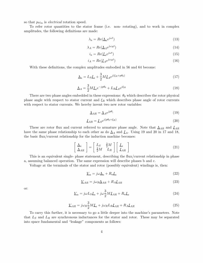
so that pωm is electrical rotation speed.To refer rotor quantities to the stator frame (i.e. non- rotating), and to work in complex

amplitudes, the following definitions are made:

λa = Re(Λaejωt) (13)

λA = Re(ΛAejωRt) (14)

ia = Re(Iaejωt) (15)

i jωRtA = Re(IAe ) (16)

With these definitions, the complex amplitudes embodied in 56 and 64 become:

3Λ = L I + MI ej(ξR+pθ0)

a S a 2 A (17)

3Λ = MI e−jpθ0

A 2 a + LRIAejξR (18)

There are two phase angles embedded in these expressions: θ0 which describes the rotor physicalphase angle with respect to stator current and ξR which describes phase angle of rotor currentswith respect to stator currents. We hereby invent two new rotor variables:

ΛAR = ΛAejpθ) (19)

I jAR = IAe

(pθ0+ξR) (20)

These are rotor flux and current referred to armature phase angle. Note that ΛAR and IAR

have the same phase relationship to each other as do ΛA and IA. Using 19 and 20 in 17 and 18,the basic flux/current relationship for the induction machine becomes:

[

Λa

] [

L 3

= S M2Λ 3

AR M L2 R

] [

Ia (21)IAR

]

This is an equivalent single- phase statement, describing the flux/current relationship in phasea, assuming balanced operation. The same expression will describe phases b and c.

Voltage at the terminals of the stator and rotor (possibly equivalent) windings is, then:

V a = jωΛa +RaIa (22)

V AR = jωRΛAR +RAIAR (23)

or:3

V a = jωLSIa + jω MIAR +RaIa (24)2

3V AR = jωR MIa + jωRLRIAR +RAIAR (25)

2

To carry this further, it is necessary to go a little deeper into the machine’s parameters. Notethat LS and LR are synchronous inductances for the stator and rotor. These may be separatedinto space fundamental and “leakage” components as follows:

4

3 4 µ RS = La − 0 lN2

L Lab = Sk2S + LSl (26)

2 π p2g

3 4 µLR = LA − 0RlN

2

L Rk2R

AB = + LRl (27)2 π p2g

Where the normal set of machine parameters holds:

R is rotor radiusl is active lengthg is the effective air- gapp is the number of pole- pairsN represents number of turnsk represents the winding factorS as a subscript refers to the statorR as a subscript refers to the rotorLl is “leakage” inductance

The two leakage terms LSl and LRl contain higher order harmonic stator and rotor inductances,slot inducances, end- winding inductances and, if necessary, a provision for rotor skew. Essentially,they are used to represent all flux in the rotor and stator that is not mutually coupled.

In the same terms, the stator- to- rotor mutual inductance, which is taken to comprise only aspace fundamental term, is:

4 µ0RlNSNRkSkRM = (28)

π p2g

Note that there are, of course, space harmonic mutual flux linkages. If they were to be included,they would hair up the analysis substantially. We ignore them here and note that they do have aneffect on machine behavior, but that effect is second- order.

Air- gap permeance is defined as:

4 µ0Rl℘ag = (29)

π p2g

so that the inductances are:

3LS = ℘agk

2

2 SN2S + LSl (30)

3LR = ℘ 2 2

agkRNR + LRl (31)2

M = ℘agNSNRkSkR (32)

Here we define “slip” s by:

ωR = sω (33)

5

so that

pωs = 1 − m

(34)ω

Then the voltage balance equations become:

V a = jω

(

3 3℘agk

2SN

2S + LSl

)

Ia + jω ℘agNSNRkSkRI R2 AR + aIa (35)

2

3 3V = jsω ℘ N N k k I + jsω

(

℘ k2 2AR ag S R S R ag

2 a 2 RNR + LRl

)

IAR +RAIAR (36)

At this point, we are ready to define rotor current referred to the stator. This is done byassuming an effective turns ratio which, in turn, defines an equivalent stator current to producethe same fundamental MMF as a given rotor current:

NRkRI2 = I

N k AR (37)S S

Now, if we assume that the rotor of the machine is shorted so that V AR = 0 and do somemanipulation we obtain:

V a = j(XM +X1)Ia + jXM I2 +RaIa (38)

R20 = jXM Ia + j(XM +X2)I2 + I2 (39)

s

where the following definitions have been made:

3XM = ω℘ 2 2

agN2 SkS (40)

X1 = ωLSl (41)

(

NSk2

SX2 = ωLRl

NRkR

)

(42)

N 2SkS

R2 = RA

(

NRkR

)

(43)

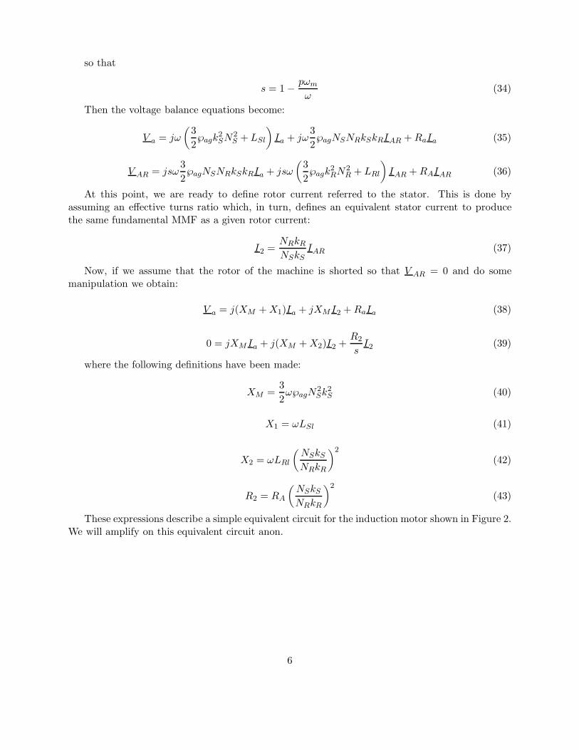
These expressions describe a simple equivalent circuit for the induction motor shown in Figure 2.We will amplify on this equivalent circuit anon.

6

∧ ∧ ∧∨ ∨

Ra ∩∩∩∩X1

∩∩∩∩X2

⊃⊃⊃⊃Xm

<<<

>>

R2s

-

Ia

I2

Figure 2: Equivalent Circuit

3 Operation: Energy Balance

Now we are ready to see how the induction machine actually works. Assume for the momentthat Figure 2 represents one phase of a polyphase system and that the machine is operated underbalanced conditions and that speed is constant or varying only slowly. “Balanced conditions” meansthat each phase has the same terminal voltage magnitude and that the phase difference betweenphases is a uniform. Under those conditions, we may analyze each phase separately (as if it werea single phase system). Assume an RMS voltage magnitude of Vt across each phase.

The “gap impedance”, or the impedance looking to the right from the right-most terminal ofX1 is:

R2Zg = jXm||(jX2 + ) (44)

s

A total, or terminal impedance is then

Zt = jX1 +Ra + Zg (45)

and terminal current isVt

It = (46)Zt

Rotor current is found by using a current divider:

jXmI2 = It (47)

jX2 + R2 + jXms

“Air-gap” power is then calculated (assuming a three-phase machine):

Pag = 3|I2|2R2

(48)s

This is real (time-average) power crossing the air-gap of the machine. Positive slip implies rotorspeed less than synchronous and positive air-gap power (motor operation). Negative slip meansrotor speed is higher than synchronous, negative air-gap power (from the rotor to the stator) andgenerator operation.

Now, note that this equivalent circuit represents a real physical structure, so it should be possibleto calculate power dissipated in the physical rotor resistance, and that is:

Ps = Pags (49)

7

(Note that, since both Pag and s will always have the same sign, dissipated power is positive.)The rest of this discussion is framed in terms of motor operation, but the conversion to generator

operation is simple. The difference between power crossing the air-gap and power dissipated in therotor resistance must be converted from mechanical form:

Pm = Pag − Ps (50)

and electrical input power is:Pin = Pag + Pa (51)

where armature dissipation is:Pa = 3|It|2Ra (52)

Output (mechanical) power isP = P P (53)out ag − w

Where Pw describes friction, windage and certain stray losses which we will discuss later.And, finally, efficiency and power factor are:

Poutη = (54)Pin

Pincosψ = (55)3VtIt

3.1 Example of Operation

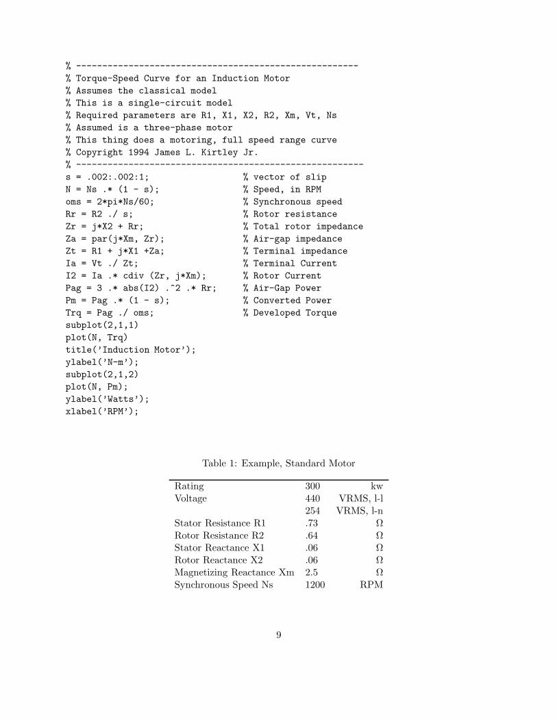
The following MATLAB script generates a torque-speed and power-speed curve for the simpleinduction motor model described above. Note that, while the analysis does not require that anyof the parameters, such as rotor resistance, be independent of rotor speed, this simple script doesassume that all parameters are constant.

3.2 Example

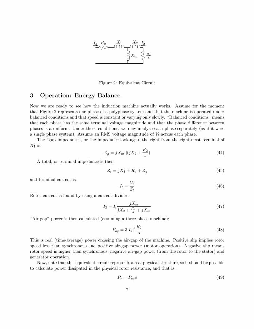
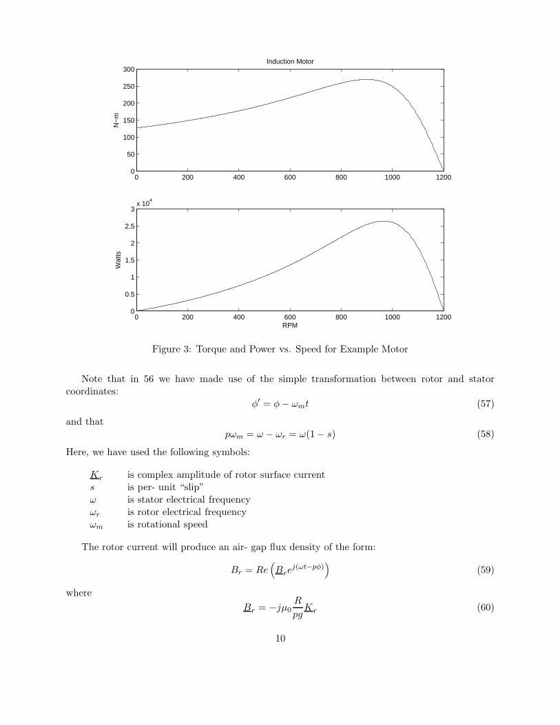
That MATLAB script has been run for a standard motor with parameters given in Table 1.Torque vs. speed and power vs. speed are plotted for this motor in Figure 3. These curves were

generated by the MATLAB script shown above.

4 Squirrel Cage Machine Model

Now we derive a circuit model for the squirrel-cage motor using field analytical techniques. Themodel consists of two major parts. The first of these is a description of stator flux in terms of statorand rotor currents. The second is a description of rotor current in terms of air- gap flux. The resultof all of this is a set of expressions for the elements of the circuit model for the induction machine.

To start, assume that the rotor is symmetrical enough to carry a surface current, the funda-mental of which is:

K = ı Re(

K ej(sωt−pφ′)r z r

= ızRe

)

(

Krej(ωt−pφ)

)

(56)

8

% ------------------------------------------------------

% Torque-Speed Curve for an Induction Motor

% Assumes the classical model

% This is a single-circuit model

% Required parameters are R1, X1, X2, R2, Xm, Vt, Ns

% Assumed is a three-phase motor

% This thing does a motoring, full speed range curve

% Copyright 1994 James L. Kirtley Jr.

% -------------------------------------------------------

s = .002:.002:1; % vector of slip

N = Ns .* (1 - s); % Speed, in RPM

oms = 2*pi*Ns/60; % Synchronous speed

Rr = R2 ./ s; % Rotor resistance

Zr = j*X2 + Rr; % Total rotor impedance

Za = par(j*Xm, Zr); % Air-gap impedance

Zt = R1 + j*X1 +Za; % Terminal impedance

Ia = Vt ./ Zt; % Terminal Current

I2 = Ia .* cdiv (Zr, j*Xm); % Rotor Current

Pag = 3 .* abs(I2) .^2 .* Rr; % Air-Gap Power

Pm = Pag .* (1 - s); % Converted Power

Trq = Pag ./ oms; % Developed Torque

subplot(2,1,1)

plot(N, Trq)

title(’Induction Motor’);

ylabel(’N-m’);

subplot(2,1,2)

plot(N, Pm);

ylabel(’Watts’);

xlabel(’RPM’);

Table 1: Example, Standard Motor

Rating 300 kwVoltage 440 VRMS, l-l

254 VRMS, l-nStator Resistance R1 .73 ΩRotor Resistance R2 .64 ΩStator Reactance X1 .06 ΩRotor Reactance X2 .06 ΩMagnetizing Reactance Xm 2.5 ΩSynchronous Speed Ns 1200 RPM

9

0 200 400 600 800 1000 12000

50

100

150

200

250

300Induction Motor

N−

m

0 200 400 600 800 1000 12000

0.5

1

1.5

2

2.5

3x 10

4

Wat

ts

RPM

Figure 3: Torque and Power vs. Speed for Example Motor

Note that in 56 we have made use of the simple transformation between rotor and statorcoordinates:

φ′ = φ− ωmt (57)

and thatpωm = ω − ωr = ω(1 − s) (58)

Here, we have used the following symbols:

Kr is complex amplitude of rotor surface currents is per- unit “slip”ω is stator electrical frequencyωr is rotor electrical frequencyωm is rotational speed

The rotor current will produce an air- gap flux density of the form:

Br = Re(

Brej(ωt−pφ)

)

(59)

whereR

Br = −jµ0 Kpg r (60)

10

Note that this describes only radial magnetic flux density produced by the space fundamentalof rotor current. Flux linked by the armature winding due to this flux density is:

λAR = lNSkS

∫ 0

Br(φ)Rdφ (61)π

−p

This yields a complex amplitude for λAR:

λAR = Re(

ΛARejωt)

(62)

where2lµ0R

2NSkSΛAR = K

p2g r (63)

Adding this to flux produced by the stator currents, we have an expression for total stator flux:

(

3 4 µ lk20N

2SR S

)

2lµ R20 NSkS

Λa = + LSl I +2 π p2g a K 4

2g r (6 )p

Expression 64 motivates a definiton of an equivalent rotor current I2 in terms of the spacefundamental of rotor surface current density:

π RI2 = K

3 NSkz (65)

S

Then we have the simple expression for stator flux:

Λa = (Lad + LSl)Ia + LadI2 (66)

where Lad is the fundamental space harmonic component of stator inductance:

3 4 µ0N2

L Sk2SRl

ad = (67)2 π p2g

4.1 Effective Air-Gap: Carter’s Coefficient

In induction motors, where the air-gap is usually quite small, it is necessary to correct the air-gappermeance for the effect of slot openings. These make the permeance of the air-gap slightly smallerthan calculated from the physical gap, effectively making the gap a bit bigger. The ratio of effectiveto physical gap is:

t+ sg = g (68)eff t+ s− gf(α)

wheres

f(α) = f

(

2g

)

= α tan(α) − log secα (69)

11

4.2 Squirrel Cage Currents

The second part of this derivation is the equivalent of finding a relationship between rotor flux andI2. However, since this machine has no discrete windings, we must focus on the individual rotorbars.

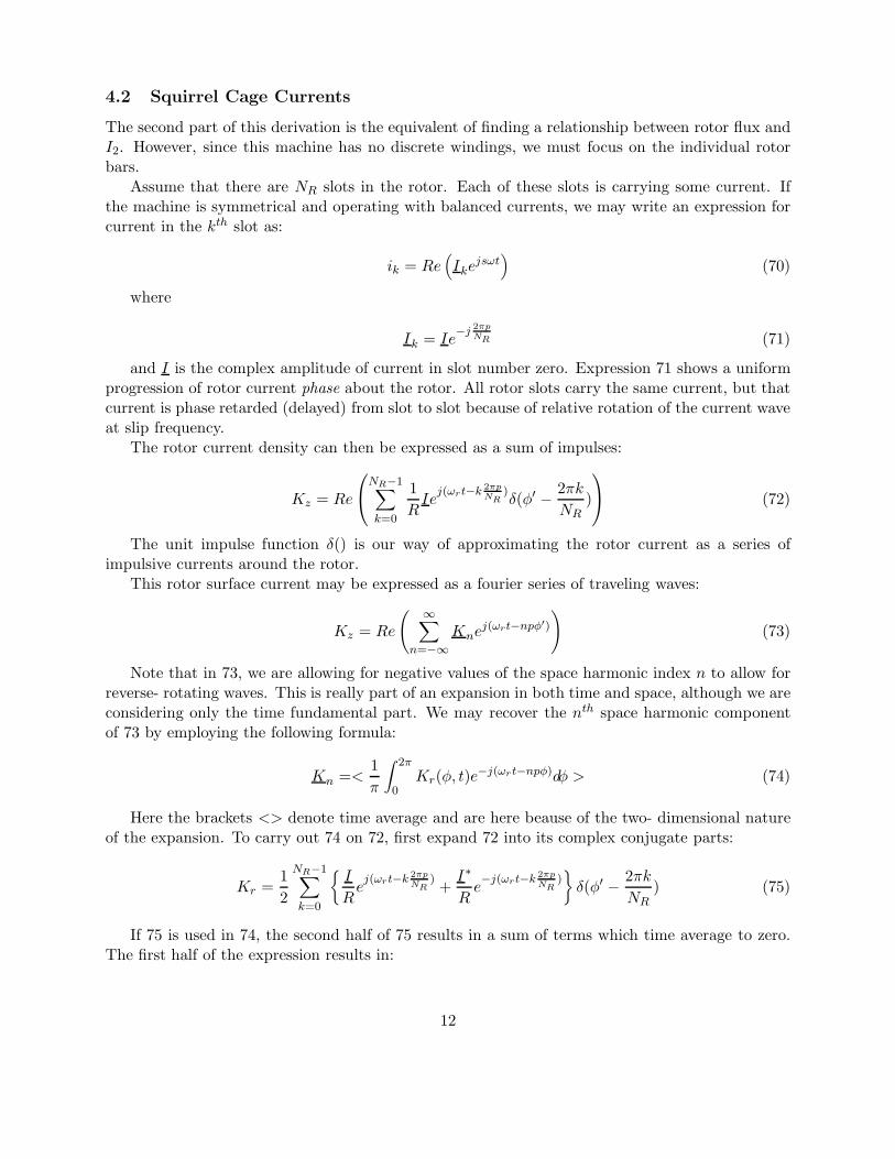
Assume that there are NR slots in the rotor. Each of these slots is carrying some current. Ifthe machine is symmetrical and operating with balanced currents, we may write an expression forcurrent in the kth slot as:

ik = Re(

Ikejsωt

)

(70)

where

2πp−j

I = Ie NRk (71)

and I is the complex amplitude of current in slot number zero. Expression 71 shows a uniformprogression of rotor current phase about the rotor. All rotor slots carry the same current, but thatcurrent is phase retarded (delayed) from slot to slot because of relative rotation of the current waveat slip frequency.

The rotor current density can then be expressed as a sum of impulses:

Kz = Re

N −R 1

∑ 1 2πpj(ω − ) ′

2πI rt k

Nk

e R δ(φR

k=0

− )NR

(72)

The unit impulse function δ() is our way of approximating the

rotor current as a series ofimpulsive currents around the rotor.

This rotor surface current may be expressed as a fourier series of traveling waves:

∞

K = Re

(

∑

K ej(ω t−n ′r pφ )

z n

n=−∞

)

(73)

Note that in 73, we are allowing for negative values of the space harmonic index n to allow forreverse- rotating waves. This is really part of an expansion in both time and space, although we areconsidering only the time fundamental part. We may recover the nth space harmonic componentof 73 by employing the following formula:

1∫ 2π

Kn =< K t )r(φ, )e−j(ωrt−npφ dφ > (74)

π 0

Here the brackets <> denote time average and are here beause of the two- dimensional natureof the expansion. To carry out 74 on 72, first expand 72 into its complex conjugate parts:

N −1 R 1

Kr =2

k

∑

=0

I 2πp 2πpj(ωrt−k ) I∗ −j(ωe NR + e rt−k )

NR

R R

δ(φ′2πk− ) (75)NR

If 75 is used in 74, the second half of 75 results in a sum of terms which time average to zero.The first half of the expression results in:

12

NI 2

Kn =

∫ −π R 1∑ 2πpk

−j npφ 2πke NR ej δ(φ

2πR 0 k=0

− )dφ (76)NR

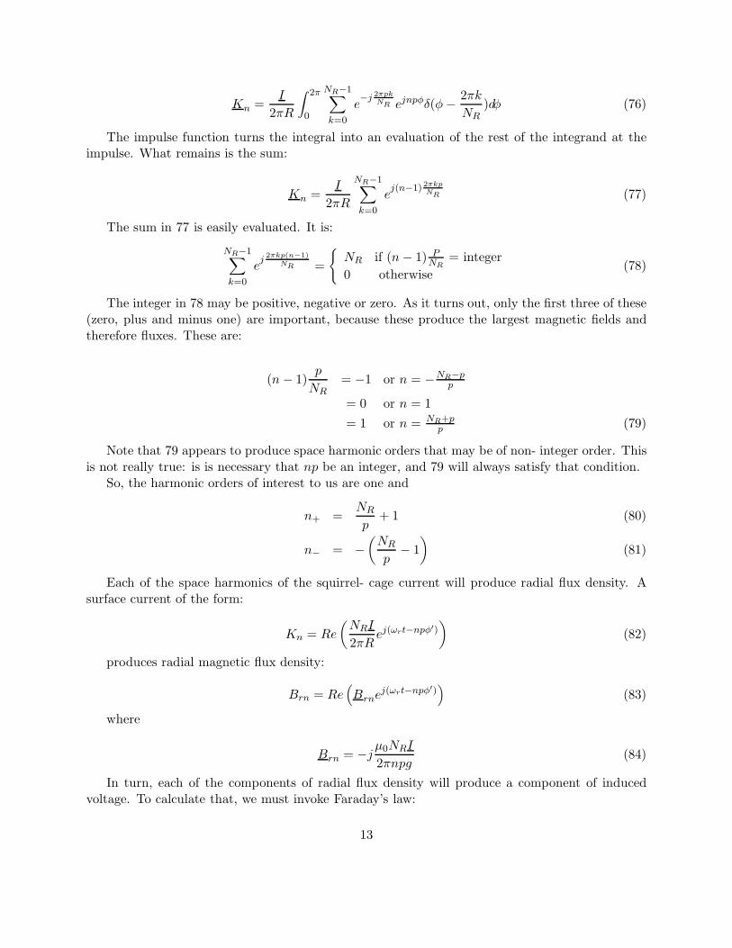
The impulse function turns the integral into an evaluation of the rest of the integrand at theimpulse. What remains is the sum:

N −1I R 2πkp

j(n−1)Kn = e NR (77)

2πRk

∑

=0

The sum in 77 is easily evaluated. It is:

N −R 1−

∑2πkp(n 1)

j N PR i

e Nf (n

R =− 1) = integer

NR (78)0 otherwise

k=0

The integer in 78 may be positive, negative or zero. As it turns out, only the first three of these(zero, plus and minus one) are important, because these produce the largest magnetic fields andtherefore fluxes. These are:

p(n − 1) = −1 or n = R

R−N −p

N p

= 0 or n = 1

= 1 or n = NR+pp

(79)

Note that 79 appears to produce space harmonic orders that may be of non- integer order. Thisis not really true: is is necessary that np be an integer, and 79 will always satisfy that condition.

So, the harmonic orders of interest to us are one and

NRn+ = + 1 (80)

p

n− = −(

NR

p− 1

)

(81)

Each of the space harmonics of the squirrel- cage current will produce radial flux density. Asurface current of the form:

NRIKn = Re

(

ej(ωrt−npφ′)

2πR

)

(82)

produces radial magnetic flux density:

Brn = Re(

Brnej(ωrt−npφ′)

)

(83)

where

µ0NRIBrn = −j (84)

2πnpg

In turn, each of the components of radial flux density will produce a component of inducedvoltage. To calculate that, we must invoke Faraday’s law:

13

∂B∇× E = − (85)∂t

The radial component of 85, assuming that the fields do not vary with z, is:

1 ∂ ∂BrEz =

R ∂φ− (86)∂t

Or, assuming an electric field component of the form:

Ezn = Re Enej(ωrt−npφ) (87)

Using 84 and 87 in 86, we obtain an expres

(

sion for electri

)

c field induced by components of air-gap flux:

ωrREn = B

np n (88)

µ0NRωrREn = −j I (89)

2πg(np)2

Now, the total voltage induced in a slot pushes current through the conductors in that slot. Wemay express this by:

E1 + En− +En+ = ZslotI (90)

Now: in 90, there are three components of air- gap field. E1 is the space fundamental field,produced by the space fundamental of rotor current as well as by the space fundamental of statorcurrent. The other two components on the left of 90 are produced only by rotor currents andactually represent additional reactive impedance to the rotor. This is often called zigzag leakageinductance. The parameter Zslot represents impedance of the slot itself: resistance and reactanceassociated with cross- slot magnetic fields. Then 90 can be re-written as:

µ0NRωrR 1 1E1 = ZslotI + j +

2πg

(

I (91)(n p)2+ (n−p)2

)

To finish this model, it is necessary to translate 91 back to the stator. See that 65 and 77 makethe link between I and I2:

NRI2 = I (92)

6NSkS

Then the electric field at the surface of the rotor is:

[

6NSkS 3 µ0NSkSR(

1 1E1 = Zs ot + jωr +

N l I (93)R π g (n+p)2 (n p)2

)]

2−

This must be translated into an equivalent stator voltage. To do so, we use 88 to translate 93into a statement of radial magnetic field, then find the flux liked and hence stator voltage fromthat. Magnetic flux density is:

14

pEBr = 1

ωrR[

6NSkSp(

Rslot 3 µ0NSkSp 1 1= + jLslot + j

NRR ωr

)

π g

(

+(n+p)2 (n−p)2

)]

I2 (94

where the slot impedance has been expressed by its real and imaginary parts:

Zslot = Rslot + jωrLslot (95

Flux linking the armature winding is:

0

λag = NSkSlR

∫

Re(

B φ)re

j(ωt−p)

dφ (96π

−2p

Which becomes:λ jωt

ag = Re(

Λage (97

where:

)

2NSkSlRΛag = j B

p r (98

Then “air- gap” voltage is:

2ωNSkSlRV ag = jωΛag = − B

p r

2

−[

12lN2Sk

2S

(

R 22 6 µ0RlN

= I jωL SkS 1 12 slot +

NR s

)

+ jω + (99π g

(

(n 2+p) (n−p)2

)

]

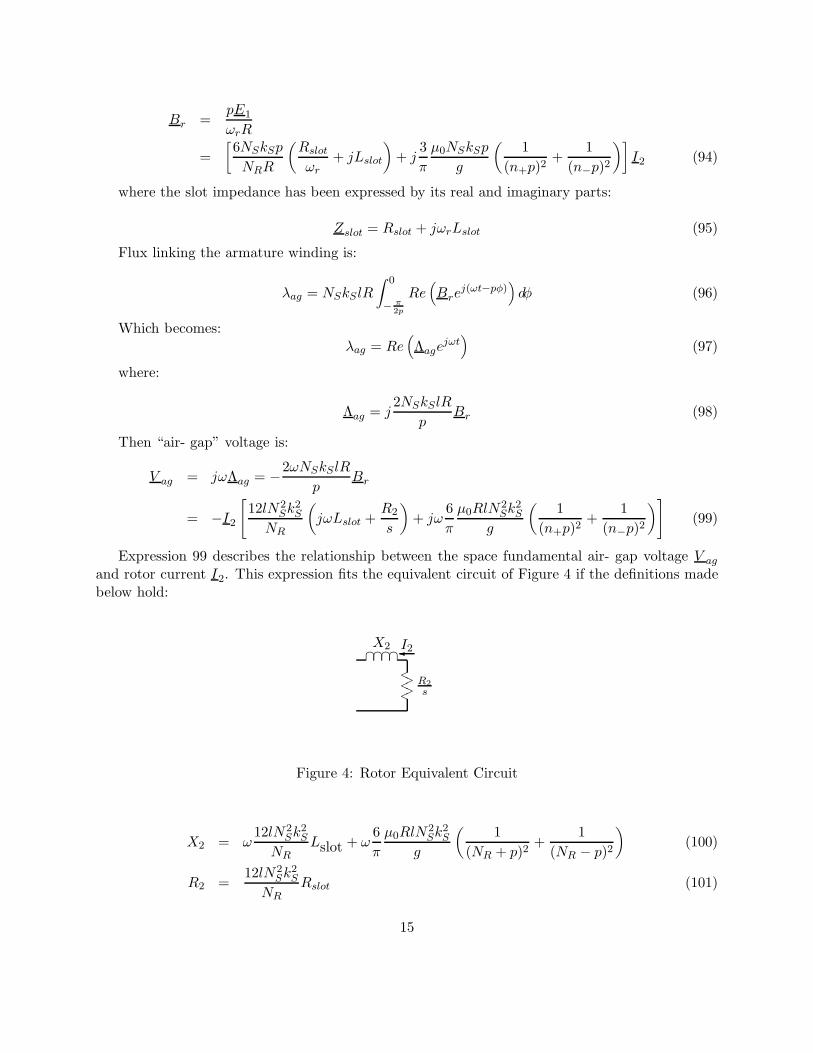
Expression 99 describes the relationship between the space fundamental air- gap voltage V a

and rotor current I2. This expression fits the equivalent circuit of Figure 4 if the definitions madbelow hold:

X2 I∩∩∩∩

2

<> R< 2> s<

Figure 4: Rotor Equivalent Circuit

12lN2k2 6 µ0RlN2k2 1 1

X L S2 = ω S S + ω S

(

+ (100slotN π g NR + p)2R ( (NR − p)2

)

12lN2

R2 = Sk2SRslot (101

NR

15

)

)

)

)

)

)

g

e

)

)

The first term in 100 expresses slot leakage inductance for the rotor. Similarly, 101 expressesrotor resistance in terms of slot resistance. Note that Lslot and Rslot are both expressed per unitlength. The second term in 100 expresses the “zigzag” leakage inductance resulting from harmonicson the order of rotor slot pitch.

Next, see that armature flux is just equal to air- gap flux plus armature leakage inductance.That is, 66 could be written as:

Λa = Λag + LalIa (102)

4.3 Stator Leakage

There are a number of components of stator leakage Lal, each representing flux paths that do notdirectly involve the rotor. Each of the components adds to the leakage inductance. The mostprominent components of stator leakage are referred to as slot, belt, zigzag, end winding, and skew.Each of these will be discussed in the following paragraphs.

4.3.1 Belt Leakage

Belt and zigzag leakage components are due to air- gap space harmonics. As it turns out, theseare relatively complicated to estimate, but we may get some notion from our first- order view ofthe machine. The trouble with estimating these leakage components is that they are not really

independent of the rotor, even though we call them “leakage”. Belt harmonics are of order n = 5and n = 7. If there were no rotor coupling, the belt harmonic leakage terms would be:

3 4 µ0N2Sk

25RlXag5 = ω (103)

2 π 52p2g

3 4 µ 2 20N

Xag7 = ω Sk7Rl (104)2 π 72p2g

The belt harmonics link to the rotor, however, and actually appear to be in parallel withcomponents of rotor impedance appropriate to 5p and 7p pole- pair machines. At these harmonicorders we can usually ignore rotor resistance so that rotor impedance is purely inductive. Thosecomponents are:

12lN2 2 2 2

X = ω Sk5 6 µ0RlN,5 L + ω Sk5 1 1

2 + (105)slotNR π g

(

(N p)2 (N − 5p)2R + 5 R

)

12lN2 2 2 2

X = ω Sk7 6 µ0RlN,7 L + ω Sk7 1 1

2 + (106)slotNR π g

(

(N + 7p)2 (NR − 7p)2R

)

In the simple model of the squirrel cage machine, because the rotor resistances are relativelysmall and slip high, the effect of rotor resistance is usually ignored. Then the fifth and seventhharmonic components of belt leakage are:

X5 = Xag5‖X2,5 (107)

X7 = Xag7‖X2,7 (108)

16

4.3.2 Zigzag Leakage

Stator zigzag leakage is from those harmonics of the orders pns = Nslots ± p where Nslots.

3 4 µ 20NSRl

(

kn +Xz = ω s kn −

+ s (109)2 π g (Nslots + p)2 (N ots − p 2

sl )

)

Note that these harmonic orders do not tend to be shorted out by the rotor cage and so nodirect interaction with the cage is ordinarily accounted for.

4.3.3 Skew Effect

In order to reduce saliency effects that occur because the rotor teeth will tend to try to align withthe stator teeth, induction motor designers always use a different number of slots in the rotor andstator. There still may be some tendency to align, and this produces “cogging” torques which inturn produce vibration and noise and, in severe cases, can retard or even prevent starting. Toreduce this tendency to “cog”, rotors are often built with a little “skew”, or twist of the slots fromone end to the other. Thus, when one tooth is aligned at one end of the machine, it is un-alignedat the other end. A side effect of this is to reduce the stator and rotor coupling by just a littlefor the space fundamental but possibly by a lot for the space harmonics. This produces leakagereactance and affects coupling to the rotor. We estimate this coupling effect here. Consider a fluxdensity Br = B1 cos pθ, linking a (possibly) skewed full-pitch current path:

∫ l ∫ π + ς x2 2p p l

λ = B1 cos pθRdθdxl π

− − + ς x2 2p p l

Here, the skew in the rotor is ς electrical radians from one end of the machine to the other.Evaluation of this yields:

2B1Rl sinς

λ = 2

p ς2

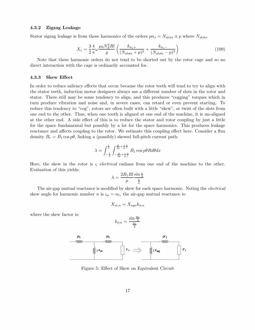
The air-gap mutual reactance is modified by skew for each space harmonic. Noting the electrical

skew angle for harmonic number n is ςn = nς, the air-gap mutual reactance is:

Xm,n = Xagnkσ,n

where the skew factor is:sin nς

kσ,n = 2nς2

j XmZ r j X r

ljX’

Z’ag

jXl jXl

Figure 5: Effect of Skew on Equivalent Circuit

17

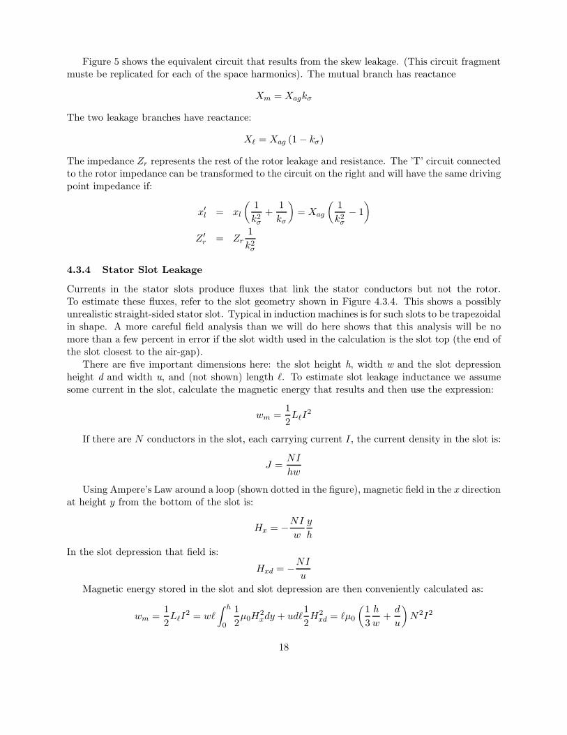
Figure 5 shows the equivalent circuit that results from the skew leakage. (This circuit fragmentmuste be replicated for each of the space harmonics). The mutual branch has reactance

Xm = Xagkσ

The two leakage branches have reactance:

Xℓ = Xag (1 − kσ)

The impedance Zr represents the rest of the rotor leakage and resistance. The ’T’ circuit connectedto the rotor impedance can be transformed to the circuit on the right and will have the same drivingpoint impedance if:

x′l = xl

(

1 1+

)

1= Xag

k2σ kσ

(

k2σ

− 1

)

Z ′1

r = Zrk2

σ

4.3.4 Stator Slot Leakage

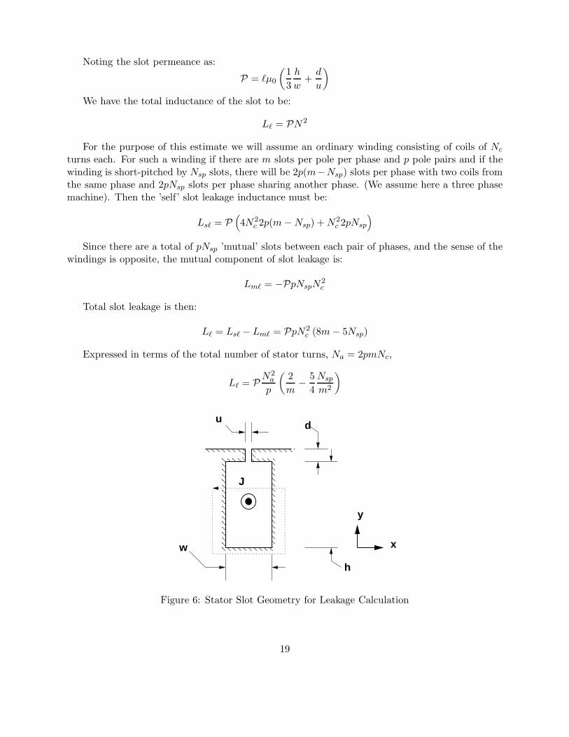
Currents in the stator slots produce fluxes that link the stator conductors but not the rotor.To estimate these fluxes, refer to the slot geometry shown in Figure 4.3.4. This shows a possiblyunrealistic straight-sided stator slot. Typical in induction machines is for such slots to be trapezoidalin shape. A more careful field analysis than we will do here shows that this analysis will be nomore than a few percent in error if the slot width used in the calculation is the slot top (the end ofthe slot closest to the air-gap).

There are five important dimensions here: the slot height h, width w and the slot depressionheight d and width u, and (not shown) length ℓ. To estimate slot leakage inductance we assumesome current in the slot, calculate the magnetic energy that results and then use the expression:

1wm = LℓI

2

2

If there are N conductors in the slot, each carrying current I, the current density in the slot is:

NIJ =

hw

Using Ampere’s Law around a loop (shown dotted in the figure), magnetic field in the x directionat height y from the bottom of the slot is:

NI yHx = −

w h

In the slot depression that field is:NI

Hxd = −u

Magnetic energy stored in the slot and slot depression are then conveniently calculated as:

1 h

w = L 2 1 2 1 2 1 h d 2 2m ℓI = wℓ

∫

µ0Hxdy + udℓ Hxd = ℓµ02

(

+0 3 w u

)

N I2 2

18

Noting the slot permeance as:

P = ℓµ0

(

1 h d+

3 w u

)

We have the total inductance of the slot to be:

Lℓ = PN2

For the purpose of this estimate we will assume an ordinary winding consisting of coils of Nc

turns each. For such a winding if there are m slots per pole per phase and p pole pairs and if thewinding is short-pitched by Nsp slots, there will be 2p(m−Nsp) slots per phase with two coils fromthe same phase and 2pNsp slots per phase sharing another phase. (We assume here a three phasemachine). Then the ’self’ slot leakage inductance must be:

Lsℓ = P(

4N2c 2p(m−Nsp) +N2

c 2pNsp

)

Since there are a total of pNsp ’mutual’ slots between each pair of phases, and the sense of thewindings is opposite, the mutual component of slot leakage is:

Lmℓ = −PpNspN2c

Total slot leakage is then:

Lℓ = Lsℓ − Lmℓ = PpN2c (8m− 5Nsp)

Expressed in terms of the total number of stator turns, Na = 2pmNc,

N2

L = a 2 5Nspℓ P

p

(

m−

4 m2

)

y

h

du

w

J

x

Figure 6: Stator Slot Geometry for Leakage Calculation

19

4.3.5 End Winding Leakage

The final component of leakage reactance is due to the end windings. This is perhaps the mostdifficult of the machine parameters to estimate, being essentially three-dimensional in nature. Thereare a number of ways of estimating this parameter, but for our purposes we will use a simplifiedparameter from Alger[1]:

14 q µ0RN2

Xe = a (p4π2 2 p2

− 0.3)

As with all such formulae, extreme care is required here, since we can give little guidance as towhen this expression is correct or even close. And we will admit that a more complete treatmentof this element of machine parameter construction would be an improvement.

4.4 Stator Winding Resistance

Estimating stator winding resistance is fairly straightforward once end winding geometry is known.Total length of the armature winding is, per phase:

ℓw = Na2 (ℓ+ ℓe)

Estimating ℓe, the length of one end winding, requires knowing how the winding is laid out andis beyond our scope here. (But once you see it you will know that length.)

The area of the winding may be estimated by knowing wire diameter and how many strandsare in parallel:

πAw = d2

4 wNinh

The area of the winding is related to slot area by a winding factor:

2NcAwλa =

Aslot

Winding resistance, per phase, is simply

ℓwRa =

σAw

where σ is wire conductivity. Note that conductivity of the materials used in induction machinesis a function of temperature and so will be winding resistance (and rotor resistance for that matter).

The Fitzgerald, Kingsley and Umans textbook[2] gives the following correction for resistance ofcopper:

T0 + TRT = Rt

T0 + t

where RT and Rt are resistances at temperatures T and t. T0 = 234.5 for copper with basicconductivity of IACS (5.8 × 107S/m)[3]. For aluminum with conductivity of 63% of IACS, T0 ≈212.9 Temperatures are given in Celcius.

20

4.5 Harmonic Order Rotor Resistance and Stray Load Losses

It is important to recognize that the machine rotor “sees” each of the stator harmonics in essentiallythe same way, and it is quite straightforward to estimate rotor parameters for the harmonic orders,as we have done just above. Now, particularly for the “belt” harmonic orders, there are rotorcurrents flowing in response to stator mmf’s at fifth and seventh space harmonic order. Theresistances attributable to these harmonic orders are:

12lN2k2

R2,5 = s 5R (110)slot,5NR

12lN2

R s k27

2,7 = R (111)slot,7NR

The higher-order slot harmonics will have relative frequencies (slips) that are:

nsn = 1 ∓ (1 − s)n

= 6k + 1

k an integer (112)n = 6k − 1

The induction motor electromagnetic interaction can now be described by an augmented mag-netic circuit as shown in Figure 21. Note that the terminal flux of the machine is the sum of all

of the harmonic fluxes, and each space harmonic is excited by the same current so the individualharmonic components are in series.

Each of the space harmonics will have an electromagnetic interaction similar to the fundamental:power transferred across the air-gap is:

Pem,n = 3I2 R2,n2,n sn

Of course dissipation in each circuit is:

Pd,n = 3I22,nR2,n

leaving

P 2 R2,nm,n = 3I2,n (1 )

n

− sns

Note that this equivalent circuit has provision for two sets of circuits which look like “cages”.In fact one of these sets is for the solid rotor body if that exists. We will discuss that anon. Thereis also a provision (rc) for loss in the stator core iron.

Power deposited in the rotor harmonic resistance elements is characterized as “stray load” lossbecause it is not easily computed from the simple machine equivalent circuit.

4.6 Slot Models

Some of the more interesting things that can be done with induction motors have to do with theshaping of rotor slots to achieve particular frequency-dependent effects. We will consider here threecases, but there are many other possibilities.

First, suppose the rotor slots are representable as being rectangular, as shown in Figure 7, andassume that the slot dimensions are such that diffusion effects are not important so that current in

21

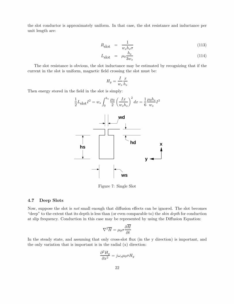
the slot conductor is approximately uniform. In that case, the slot resistance and inductance perunit length are:

1R = (113)slot wshsσ

hsL = µslot 0 (114)

3ws

The slot resistance is obvious, the slot inductance may be estimated by recognizing that if thecurrent in the slot is uniform, magnetic field crossing the slot must be:

I xHy =

ws hs

Then energy stored in the field in the slot is simply:

1 hs Ix 2

L I2 µ0 1 µ0hs= w dx = I2

slot s2 0 2 wshs 6 ws

∫ ( )

xhs

wd

hd

ws

y

Figure 7: Single Slot

4.7 Deep Slots

Now, suppose the slot is not small enough that diffusion effects can be ignored. The slot becomes“deep” to the extent that its depth is less than (or even comparable to) the skin depth for conductionat slip frequency. Conduction in this case may be represented by using the Diffusion Equation:

∇2 ∂HH = µ0σ

∂t

In the steady state, and assuming that only cross-slot flux (in the y direction) is important, andthe only variation that is important is in the radial (x) direction:

∂2Hy= jωsµ0σHy

∂x2

22

This is solved by solutions of the form:

H = H e±(1+j)x

y δ±

where the skin depth is

δ =

√

2

ωsµ0σ

Since Hy must vanish at the bottom of the slot, it must take the form:

sinh(1 + j)x

Hy = H δtop

sinh(1 + j)hs

δ

Since current is the curl of magnetic field,

∂Hy 1 + j cosh(1 + j)hs

Jz = σEz = = H δtop∂x δ sinh(1 + j)hs

δ

Then slot impedance, per unit length, is:

1 1 + j hsZ = coth(1 + j)slot ws σδ δ

Of course the impedance (purely reactive) due to the slot depression must be added to this. Itis possible to extract the real and imaginary parts of this impedance (the process is algebraically abit messy) to yield:

1 sinh 2hs + sin 2hs

R = δ δslot w σδ cosh 2hs

s δ− cos 2hs

δ

hd 1 1 sinh 2hs

L = µ + δsin 2hs

δslot 0

−wd ωs wsσδ cosh 2hs

δ− cos 2hs

δ

4.8 Arbitrary Slot Shape Model

It is possible to obtain a better model of the behavior of rotor conductor slots by using simplenumerical methods. In many cases rotor slots are shaped with the following objectives in mind:

1. A substantial part of the periphery of the rotor should be devoted to active conductor, forgood running performance.

2. The magnetic iron of the rotor must occupy a certain fraction of the periphery, to avoidsaturation.

3. For good starting performance, some means of forcing current to flow only in the top part ofthe rotor bar should be devised.

23

Generally the rotor teeth, which make up part of the machine’s magnetic circuit, are of roughlyconstant width to avoid flux concentration. The rotor conductor bars are therefore tapered, withtheir narrow ends towards the center of the rotor. To provide for current concentration on startingthey often have a ’starting bar’ at the outer periphery of the rotor with a much narrower regionwhich has high inductance just below. The bulk of the rotor bar occupies the tapered region allowedbetween the teeth.

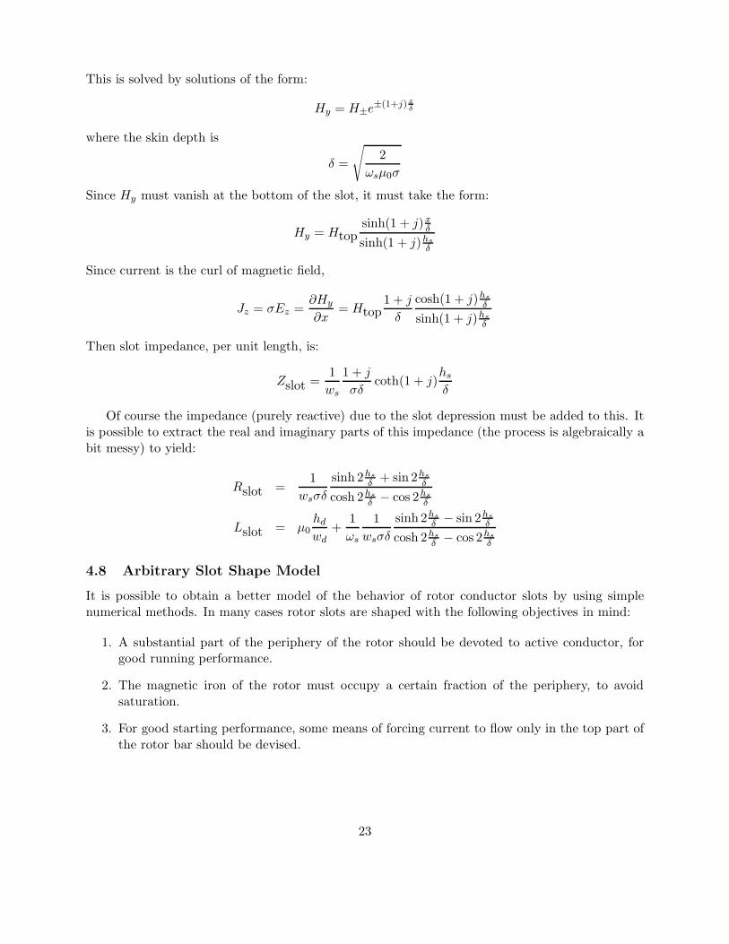
This geometry is quite a bit more complicated than that described in the previous section. Notethat, if we can describe the slot impedance per unit length as a function of frequency: Zs(ω) =Rs(ω) + jXs(ω), we can carry out the analysis of the machine as described previously. Thus ouranalysis is directed toward frequency response modeling of the rotor slot. Focusing then on a singleslot, use the notation as described in Figure 8.

w[n]

∆ x

∆ x

E [n]z

x

y z

x = n

zE [n−1]

Figure 8: Slot Geometry Notation

The impedance per unit length is the ratio between slot current and axial electric field:

EZ z

s =I

For the purpose of this analysis we will use the symbol x as the radial distance from the bottomof the slot. Assume the slot can be divided radially into a number of regions or ’slices’, each withradial height ∆x. We further assume that currents are axially (z) directed and that magnetic fieldcrosses the slot in the y direction. Under these assumptions the electric field at the top of one ofthe slices is related to the electric field at the bottom of the slice by magnetic field crossing throughthe slice. Using the trapezoidal rule for integration:

∆xEz(x) − Ez(x− ∆x) = jωµ0 +

2

(

Hy(x) Hy(x− ∆x))

The magnetic field is simply:

1 x 1Hy(x) =

∫

σw(x)Ez(x)dx =w(x) 0 wn

∑

nIn

i=1

where In is the total current flowing in one slice. Note that this can be reformulated into a laddernetwork by again using the trapezoidal rule for integration: current flowing in slice number n would

24

be:∆x

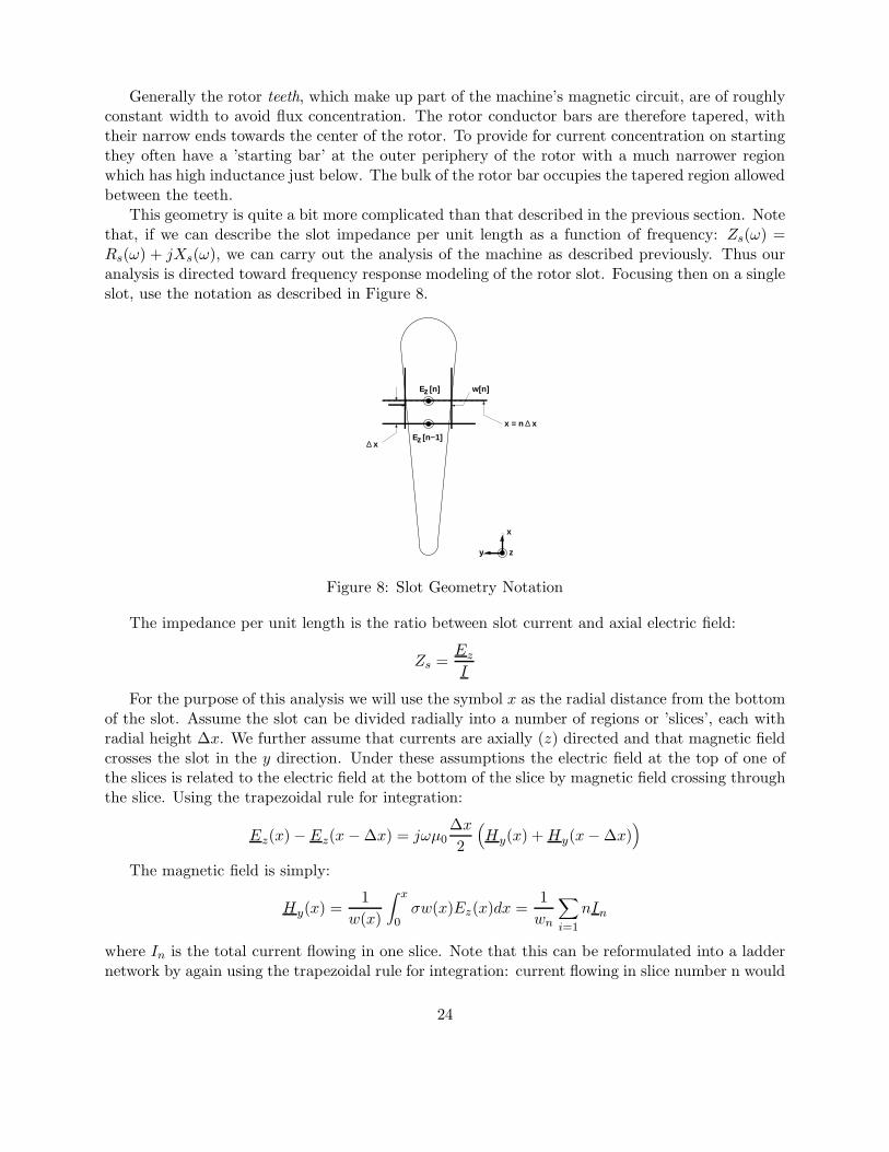
In = σ (wnEn + wn−1En−1)2Now the slot may be described as is shown in the ladder network of Figure 9. The incremental

reactance of one slice is:

2Xn = ωµ0∆x

(wn + wn−1)

and the resistance of a slice is:1 2

Rn =σ∆x wn +wn−1

L[n] L[n] L[n−1] L[n−1]

2 2 2 2

R[n] R[n−1]

Figure 9: Slot Impedance Ladder Network

The procedure is to start at the bottom of the slot, corresponding to the right-hand end of theladder (the inductance at the bottom of the slot is infinite so the first slice has only the resistance),and building toward the top of the slot.

4.9 Multiple Cages

In some larger induction motors the rotor cage is built in such a way as to separate the functionsof ’starting’ and ’running’. The purpose of a “deep” slot is to improve starting performance ofa motor. When the rotor is stationary, the frequency seen by rotor conductors is relatively high,and current crowding due to the skin effect makes rotor resistance appear to be high. As the rotoraccelerates the frequency seen from the rotor drops, lessening the skin effect and making moreuse of the rotor conductor. This, then, gives the machine higher starting torque (requiring highresistance) without compromising running efficiency.

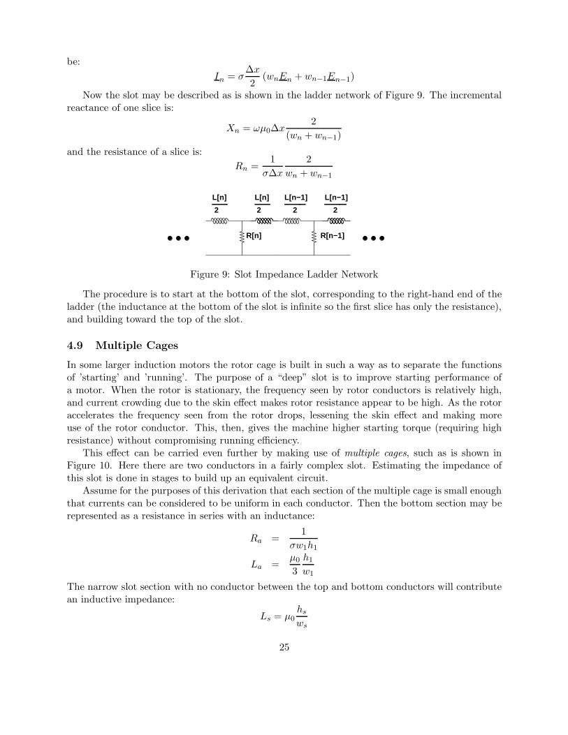
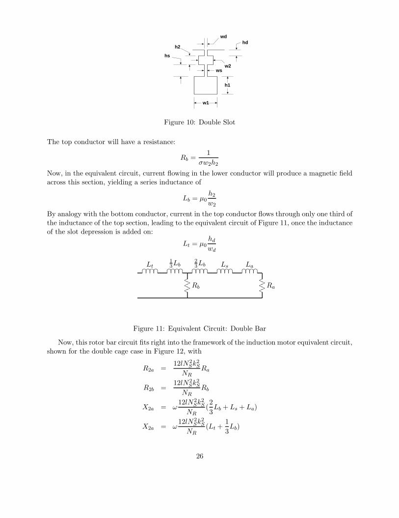
This effect can be carried even further by making use of multiple cages, such as is shown inFigure 10. Here there are two conductors in a fairly complex slot. Estimating the impedance ofthis slot is done in stages to build up an equivalent circuit.

Assume for the purposes of this derivation that each section of the multiple cage is small enoughthat currents can be considered to be uniform in each conductor. Then the bottom section may berepresented as a resistance in series with an inductance:

1Ra =

σw1h1

µ0 h1La =

3 w1

The narrow slot section with no conductor between the top and bottom conductors will contributean inductive impedance:

hsLs = µ0

ws

25

hs

ws

h2

w1

h1

w2

hdwd

Figure 10: Double Slot

The top conductor will have a resistance:

1Rb =

σw2h2

Now, in the equivalent circuit, current flowing in the lower conductor will produce a magnetic fieldacross this section, yielding a series inductance of

h2Lb = µ0

w2

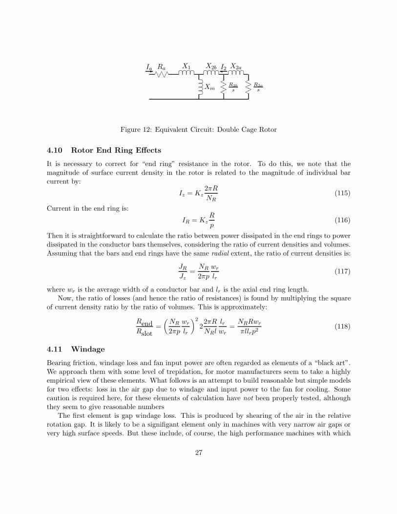
By analogy with the bottom conductor, current in the top conductor flows through only one third ofthe inductance of the top section, leading to the equivalent circuit of Figure 11, once the inductanceof the slot depression is added on:

hdLt = µ0

wd

1 2L bt

L L3 3 b Ls La∩∩∩∩ ∩∩∩∩

<

∩∩∩∩ ∩∩∩∩ ∩∩∩∩<

> >< R <> b >Ra

< <

Figure 11: Equivalent Circuit: Double Bar

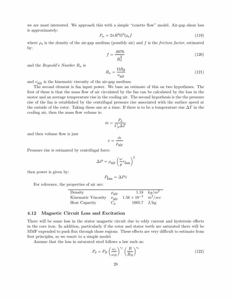
Now, this rotor bar circuit fits right into the framework of the induction motor equivalent circuit,shown for the double cage case in Figure 12, with

12lN2

R Sk2S

2a = RaNR

12lN2

R2b = Sk2SRb

NR

12lN2

X2a = ω Sk2S 2

( Lb + Ls + La)NR 3

12lN2

X2a = ω Sk2S 1

(Lt + Lb)NR 3

26

∧ ∧ ∧∨ ∨

Ra ∩∩∩∩X1

∩∩∩∩X2b

∩∩∩∩X2a

⊃⊃⊃⊃Xm

<<<

>>

R2b

s

<<<

>>

R2a

s

-

Ia

I2

Figure 12: Equivalent Circuit: Double Cage Rotor

4.10 Rotor End Ring Effects

It is necessary to correct for “end ring” resistance in the rotor. To do this, we note that themagnitude of surface current density in the rotor is related to the magnitude of individual barcurrent by:

2πRIz = Kz (115)

NR

Current in the end ring is:R

IR = Kz (116)p

Then it is straightforward to calculate the ratio between power dissipated in the end rings to powerdissipated in the conductor bars themselves, considering the ratio of current densities and volumes.Assuming that the bars and end rings have the same radial extent, the ratio of current densities is:

JR NR wr= (117)

Jz 2πp lr

where wr is the average width of a conductor bar and lr is the axial end ring length.Now, the ratio of losses (and hence the ratio of resistances) is found by multiplying the square

of current density ratio by the ratio of volumes. This is approximately:

R R)

Nend(

N w 2r 2πR lr RRwr

= 2 = (118)R 2πp lr N w l p2

Rl r π lslot r

4.11 Windage

Bearing friction, windage loss and fan input power are often regarded as elements of a “black art”.We approach them with some level of trepidation, for motor manufacturers seem to take a highlyempirical view of these elements. What follows is an attempt to build reasonable but simple modelsfor two effects: loss in the air gap due to windage and input power to the fan for cooling. Somecaution is required here, for these elements of calculation have not been properly tested, althoughthey seem to give reasonable numbers

The first element is gap windage loss. This is produced by shearing of the air in the relativerotation gap. It is likely to be a signifigant element only in machines with very narrow air gaps orvery high surface speeds. But these include, of course, the high performance machines with which

27

we are most interested. We approach this with a simple “couette flow” model. Air-gap shear lossis approximately:

Pw = 2πR4Ω3lρaf (119)

where ρa is the density of the air-gap medium (possibly air) and f is the friction factor, estimatedby:

.0076f = 1 (120)

R 4n

and the Reynold’s Number Rn isΩRg

Rn = (121)νair

and ν is the kinematic viscosity of the air-gap medium.airThe second element is fan input power. We base an estimate of this on two hypotheses. The

first of these is that the mass flow of air circulated by the fan can be calculated by the loss in themotor and an average temperature rise in the cooling air. The second hypothesis is the the pressurerise of the fan is established by the centrifugal pressure rise associated with the surface speed atthe outside of the rotor. Taking these one at a time: If there is to be a temperature rise ∆T in thecooling air, then the mass flow volume is:

Pdm =

Cp∆T

and then volume flow is justm

v =ρair

Pressure rise is estimated by centrifugal force:

∆P = ρair

(

ωrfanp

)2

then power is given by:P = ∆P vfan

For reference, the properties of air are:

Density ρ 1.18 kg/m2air

Kinematic Viscosity ν 1.56 × 10−5 m2/secairHeat Capacity Cp 1005.7 J/kg

4.12 Magnetic Circuit Loss and Excitation

There will be some loss in the stator magnetic circuit due to eddy current and hysteresis effectsin the core iron. In addition, particularly if the rotor and stator teeth are saturated there will beMMF expended to push flux through those regions. These effects are very difficult to estimate fromfirst principles, so we resort to a simple model.

Assume that the loss in saturated steel follows a law such as:(

ω)ǫf

ePd = PB

ωB

(

B1

B

)ǫb

( 22)B

28

This is not too bad an estimate for the behavior of core iron. Typically, ǫf is a bit less thantwo (between about 1.3 and 1.6) and ǫb is a bit more than two (between about 2.1 and 2.4). Ofcourse this model is good only for a fairly restricted range of flux density. Base dissipation isusually expressed in “watts per kilogram”, so we first compute flux density and then mass of thetwo principal components of the stator iron, the teeth and the back iron.

In a similar way we can model the exciting volt-amperes consumed by core iron by somethinglike:

Qc =

(

BV a1

( )ǫv1

+ V a2

(

B)ǫv2

)

ω(123)

BB BB ωB

This, too, is a form that appears to be valid for some steels. Quite obviously it may be necessaryto develop different forms of curve ’fits’ for different materials.

Flux density (RMS) in the air-gap is:

pVaBr = (124)

2RlNak1ωs

Then flux density in the stator teeth is:

wt + w1Bt = Br (125)

wt

where wt is tooth width and w1 is slot top width. Flux in the back-iron of the core is

RBc = Br (126)

pdc

where dc is the radial depth of the core.One way of handling this loss is to assume that the core handles flux corresponding to terminal

voltage, add up the losses and then compute an equivalent resistance and reactance:

3rc =

|Va|2Pcore

3|V 2a

xc =|

Qcore

then put this equivalent resistance in parallel with the air-gap reactance element in the equivalentcircuit.

5 Solid Iron Rotor Bodies

Solid steel rotor electric machines (SSRM) can be made to operate with very high surface speeds andare thus suitable for use in high RPM situations. They resemble, in form and function, hysteresismachines. However, asynchronous operation will produce higher power output because it takesadvantage of higher flux density. We consider here the interactions to be expected from solid ironrotor bodies. The equivalent circuits can be placed in parallel (harmonic-by-harmonic) with theequivalent circuits for the squirrel cage, if there is also a cage in the machine.

29

To estimate the rotor parameters R2s and X2s, we assume that important field quantities inthe machine are sinusoidally distributed in time and space, so that radial flux density is:

Br = Re(

Brej(ωt−pφ)

)

(127)

and, similarly, axially directed rotor surface current is:

K )z = Re

(

K ej(ωt−pφz

)

(128)

Now, since by Faraday’s law:∂B∇× E = − (129)∂t

we have, in this machine geometry:1 ∂ ∂B

Ez =R ∂φ

− r(130)

∂t

The transformation between rotor and stator coordinates is:

φ′ = φ− ωmt (131)

where ωm is rotor speed. Then:pωm = ω − ωr = ω(1 − s) (132)

andNow, axial electric field is, in the frame of the rotor, just:

E = Re(

E ej(ωt−pφ)z z (133)

= Re(

E ej(ω −rt pφ

)

′)z

)

(134)

andωrR

Ez = Bp r (135)

Of course electric field in the rotor frame is related to rotor surface current by:

Ez = ZsKz (136)

Now these quantities can be related to the stator by noting that air-gap voltage is related toradial flux density by:

pBr = V

2lNak1Rωag (137)

The stator-equivalent rotor current is:

π RI2 = K

3 Nakz (138)

a

Then we can find stator referred, rotor equivalent impedance to be:

V ag 3 4 l ωZ 2 2 Ez

2 = = N2 R ak2 a (139)I π ωr Kz

30

Now, if rotor surface impedance can be expressed as:

Zs = Rs + jωrLs (140)

thenR2

Z2 = + jX2 (141)s

where

3 4 lR2 = N2

s2 R ak

21R (142)

π3 4 l

X 22 = N k2Xs (143)

2 π R a 1

Now, to find the rotor surface impedance, we make use of a nonlinear eddy-current model proposedby Agarwal. First we define an equivalent penetration depth (similar to a skin depth):

2Hmδ =

√

(144)ωrσB0

where σ is rotor surface material volume conductivity, B0, ”saturation flux density” is taken to be75 % of actual saturation flux density and

3 NHm = |Kz| aka

= |I2| (145)π R

Then rotor surface resistivity and surface reactance are:

16 1Rs = (146)

3π σδXs = .5Rs (147)

Note that the rotor elements X2 and R2 depend on rotor current I2, so the problem is nonlinear.We find, however, that a simple iterative solution can be used. First we make a guess for R2 and findcurrents. Then we use those currents to calculate R2 and solve again for current. This procedureis repeated until convergence, and the problem seems to converge within just a few steps.

Aside from the necessity to iterate to find rotor elements, standard network techniques can beused to find currents, power input to the motor and power output from the motor, torque, etc.

5.1 Solution

Not all of the equivalent circuit elements are known as we start the solution. To start, we assumea value for R2, possibly some fraction of Xm, but the value chosen doesn not seem to mattermuch. The rotor reactance X2 is just a fraction of R2. Then, we proceed to compute an “air-gap”impedance, just the impedance looking into the parallel combination of magnetizing and rotorbranches:

R2Zg = jXm||(jX2 + ) (148)

s

(Note that, for a generator, slip s is negative).

31

A total impedance is thenZt = jX1 +R1 + Zg (149)

and terminal current isVt

It = (150)Zt

Rotor current is just:jXm

I2 = It (151)jX2 + R2

s

Now it is necessary to iteratively correct rotor impedance. This is done by estimating fluxdensity at the surface of the rotor using (145), then getting a rotor surface impedance using (146)and using that and (143 to estimate a new value for R2. Then we start again with (148). Theprocess “drops through” this point when the new and old estimates for R2 agree to some criterion.

5.2 Harmonic Losses in Solid Steel

If the rotor of the machine is constructed of solid steel, there will be eddy currents induced on therotor surface by the higher-order space harmonics of stator current. These will produce magneticfields and losses. This calculation assumes the rotor surface is linear and smooth and can becharacterized by a conductivity and relative permeability. In this discussion we include two spaceharmonics (positive and negative going). In practice it may be necessary to carry four (or evenmore) harmonics, including both ‘belt’ and ‘zigzag’ order harmonics.

Terminal current produces magnetic field in the air-gap for each of the space harmonic orders,and each of these magnetic fields induces rotor currents of the same harmonic order.

The “magnetizing” reactances for the two harmonic orders, really the two components of thezigzag leakage, are:

k2p

Xzp = Xm (152)N2

pk21

k2

X nzn = Xm (153)

N2nk

21

where Np and Nn are the positive and negative going harmonic orders: For ‘belt’ harmonicsthese orders are 7 and 5. For ‘zigzag’ they are:

Ns + pNp = (154)

p

NsNn =

− p(155)

p

Now, there will be a current on the surface of the rotor at each harmonic order, and following 65,the equivalent rotor element current is:

π RI2p = K 5

3 Nakp (1 6)

p

π RI2n = K 1

3 N n ( 57)akn

32

These currents flow in response to the magnetic field in the air-gap which in turn produces anaxial electric field. Viewed from the rotor this electric field is:

Ep = spωRBp (158)

En = snωRBn (159)

where the slip for each of the harmonic orders is:

sp = 1 −Np(1 − s) (160)

sn = 1 +Np(1 − s) (161)

and then the surface currents that flow in the surface of the rotor are:

EpKp = (162)

Zsp

EKn = n (163)

Zsn

where Zsp and Zsn are the surface impedances at positive and negative harmonic slip frequencies,respectively. Assuming a linear surface, these are, approximately:

1 + jZs = (164)

σδ

where σ is material restivity and the skin depth is

δ =

√

2(165)

ωsµσ

and ωs is the frequency of the given harmonic from the rotor surface. We can postulate that theappropriate value of µ to use is the same as that estimated in the nonlinear calculation of the spacefundamental, but this requires empirical confirmation.

The voltage induced in the stator by each of these space harmonic magnetic fluxes is:

2NakplRωVp = B

N p (166)pp

2NaknlRωVn = B

Nnpn (167)

Then the equivalent circuit impedance of the rotor is just:

Vp 3 4 N2ak

2pl Zsp

Z2p = = (168)Ip 2 π NpR sp

Vn 3 4 N2

Z2n = = ak2nl Zsn

(169)In 2 π NnR sn

The equivalent rotor circuit elements are now:

33

3 4 N2 2akpl 1

R2p = (170)2 π NpR σδp

3 4 N2 l 1R2n = ak

2n (171)

2 π NnR σδn

1X2p = R2p (172)

2

1X2n = R2n (173)

2

5.3 Stray Losses

So far in this document, we have outlined the major elements of torque production and consequentlyof machine performance. We have also discussed, in some cases, briefly, the major sources of lossin induction machines. Using what has been outlined in this document will give a reasonableimpression of how an induction machine works. We have also discussed some of the stray load

losses: those which can be (relatively) easily accounted for in an equivalent circuit description ofthe machine. But there are other losses which will occur and which are harder to estimate. We donot claim to do a particularly accurate job of estimating these losses, and fortunately they do notnormally turn out to be very large. To be accounted for here are:

1. No-load losses in rotor teeth because of stator slot opening modulation of fundamental fluxdensity,

2. Load losses in the rotor teeth because of stator zigzag mmf, and

3. No-load losses in the solid rotor body (if it exists) due to stator slot opening modulation offundamental flux density.

Note that these losses have a somewhat different character from the other miscellaneous losses wecompute. They show up as drag on the rotor, so we subtract their power from the mechanicaloutput of the machine. The first and third of these are, of course, very closely related so we takethem first.

The stator slot openings ‘modulate’ the space fundamental magnetic flux density. We mayestimate a slot opening angle (relative to the slot pitch):

2πwdNs wdNsθD = =

2πr r

Then the amplitude of the magnetic field disturbance is:

2 θDBH = Br1 sin

π 2

In fact, this flux disturbance is really in the form of two traveling waves, one going forward and onebackward with respect to the stator at a velocity of ω/Ns. Since operating slip is relatively small,

34

the two variations will have just about the same frequency as viewed from the rotor, so it seemsreasonable to lump them together. The frequency is:

NsωH = ω

p

Now, for laminated rotors this magnetic field modulation will affect the tips of rotor teeth. Weassume (perhaps arbitrarily) that the loss due to this magnetic field modulation can be estimatedfrom ordinary steel data (as we estimated core loss above) and that only the rotor teeth, not any ofthe rotor body, are affected. The method to be used is straightforward and follows almost exactlywhat was done for core loss, with modification only of the frequency and field amplitude.

For solid steel rotors the story is only a little different. The magnetic field will produce an axialelectric field:

ωEz = R BH

p

and that, in turn, will drive a surface current

EKz = z

Zs

Now, what is important is the magnitude of the surface current, and since√

|Zs| = 1 + .52Rs ≈1.118Rs, we can simply use rotor resistance. The nonlinear surface penetration depth is:

δ =

√

2B0

ωHσ|Kz|

A brief iterative substitution, re-calculating δ and then |Kz| quickly yields consistent values for δand Rs. Then the full-voltage dissipation is:

2

Prs = 2 Rl|K

π z|σδ

and an equivalent resistance is:3

Rrs =|Va|2Prs

Finally, the zigzag order current harmonics in the stator will produce magnetic fields in theair gap which will drive magnetic losses in the teeth of the rotor. Note that this is a bit differentfrom the modulation of the space fundamental produced by the stator slot openings (although theharmonic order will be the same, the spatial orientation will be different and will vary with loadcurrent). The magnetic flux in the air-gap is most easily related to the equivalent circuit voltageon the nth harmonic:

npvnBn =

2lRNaknω

This magnetic field variation will be substantial only for the zigzag order harmonics: the beltharmonics will be essentially shorted out by the rotor cage and those losses calculated withinthe equivalent circuit. The frequency seen by the rotor is that of the space harmonics, alreadycalculated, and the loss can be estimated in the same way as core loss, although as we have pointedout it appears as a ‘drag’ on the rotor.

35

6 Induction Motor Speed Control

6.1 Introduction

The inherent attributes of induction machines make them very attractive for drive applications.They are rugged, economical to build and have no sliding contacts to wear. The difficulty withusing induction machines in servomechanisms and variable speed drives is that they are “hard tocontrol”, since their torque-speed relationship is complex and nonlinear. With, however, modernpower electronics to serve as frequency changers and digital electronics to do the required arithmetic,induction machines are seeing increasing use in drive applications.

In this chapter we develop models for control of induction motors. The derivation is quite brieffor it relies on what we have already done for synchronous machines. In this chapter, however, wewill stay in “ordinary” variables, skipping the per-unit normalization.

6.2 Volts/Hz Control

Remembering that induction machines generally tend to operate at relatively low per unit slip, wemight conclude that one way of building an adjustable speed drive would be to supply an inductionmotor with adjustable stator frequency. And this is, indeed, possible. One thing to remember isthat flux is inversely proportional to frequency, so that to maintain constant flux one must makestator voltage proportional to frequency (hence the name “constant volts/Hz”). However, voltagesupplies are always limited, so that at some frequency it is necessary to switch to constant voltagecontrol. The analogy to DC machines is fairly direct here: below some “base” speed, the machineis controlled in constant flux (“volts/Hz”) mode, while above the base speed, flux is inverselyproportional to speed. It is easy to see that the maximum torque is then inversely to the square offlux, or therefore to the square of frequency.

To get a first-order picture of how an induction machine works at adjustable speed, start withthe simplified equivalent network that describes the machine, as shown in Figure 13

Ia Ra X1 X2-

I2∧ ∧ ∧∨ ∨

∩∩∩∩ ∩∩∩∩⊃⊃ <

⊃X > R< 2

⊃ m > s<

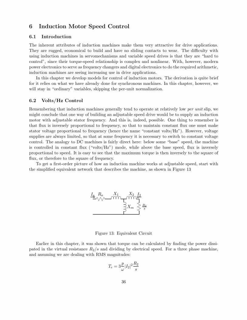
Figure 13: Equivalent Circuit

Earlier in this chapter, it was shown that torque can be calculated by finding the power dissi-pated in the virtual resistance R2/s and dividing by electrical speed. For a three phase machine,and assuming we are dealing with RMS magnitudes:

pTe = 3

ω|I2|2

R2

s

36

where ω is the electrical frequency and p is the number of pole pairs. It is straightforward to findI2 using network techniques. As an example, Figure 14 shows a series of torque/speed curves foran induction machine operated with a wide range of input frequencies, both below and above its“base” frequency. The parameters of this machine are:

Number of Phases 3Number of Pole Pairs 3RMS Terminal Voltage (line-line) 230Frequency (Hz) 60Stator Resistance R1 .06 ΩRotor Resistance R2 .055 ΩStator Leakage X1 .34 ΩRotor Leakage X2 .33 ΩMagnetizing Reactance Xm 10.6 Ω

Strategy for operating the machine is to make terminal voltage magnitude proportional to frequencyfor input frequencies less than the “Base Frequency”, in this case 60 Hz, and to hold voltage constantfor frequencies above the “Base Frequency”.

0 50 100 150 200 2500

50

100

150

200

250

Induction Motor Torque

N−

m

Speed, RPM

Figure 14: Induction Machine Torque-Speed Curves

For high frequencies the torque production falls fairly rapidly with frequency (as it turns out,it is roughly proportional to the inverse of the square of frequency). It also falls with very lowfrequency because of the effects of terminal resistance. We will look at this next.

6.3 Idealized Model: No Stator Resistance

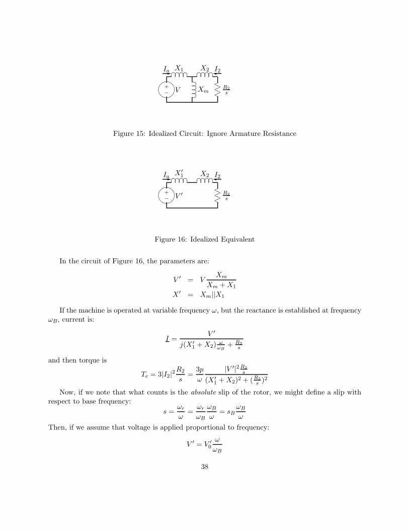
Ignore, for the moment, R1. An equivalent circuit is shown in Figure 15. It is fairly easy to showthat, from the rotor, the combination of source, armature leakage and magnetizing branch can bereplaced by its equivalent circuit, as shown in in Figure 16.

37

+−

V

∩∩∩∩X1

∩∩∩∩X2

⊃⊃⊃⊃Xm

<<<

>>

R2s

-

Ia

I2

Figure 15: Idealized Circuit: Ignore Armature Resistance

+− V ′

∩∩∩∩X ′

1∩∩∩∩X2

<<<

>>

R2s

-Ia

I2

Figure 16: Idealized Equivalent

In the circuit of Figure 16, the parameters are:

V ′Xm

= VXm +X1

X ′ = Xm||X1

If the machine is operated at variable frequency ω, but the reactance is established at frequencyωB, current is:

V ′

I =j(X ′

1 +X2)ω

ω+ R2

B s

and then torque isR 3p

Te = 3|V ′|2 R2

| | 2I 22 = s

s ω (X ′1 +X2)2 + (R2

s)2

Now, if we note that what counts is the absolute slip of the rotor, we might define a slip withrespect to base frequency:

ωr ωr ωB ωBs = = = sB

ω ωB ω ω

Then, if we assume that voltage is applied proportional to frequency:

V ′ = V ′ω

0 ωB

38

and with a little manipulation, we get:

|V ′|2 R3p 2

0 sTe = B

ωB (X ′1 +X2)2 + (R2

s)2

B

This would imply that torque is, if voltage is proportional to frequency, meaning constant appliedflux, dependent only on absolute slip. The torque-speed curve is a constant, dependent only on thedifference between synchronous and actual rotor speed.

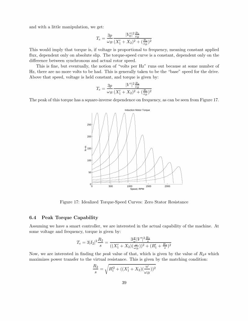
This is fine, but eventually, the notion of “volts per Hz” runs out because at some number ofHz, there are no more volts to be had. This is generally taken to be the “base” speed for the drive.Above that speed, voltage is held constant, and torque is given by:

|V ′|2 R3p 2

sTe = B

ωB (X ′1 +X 2 R2 2

2) + ( )sB

The peak of this torque has a square-inverse dependence on frequency, as can be seen from Figure 17.

0 500 1000 1500 20000

50

100

150

200

250

Induction Motor Torque

N−

m

Speed, RPM

Figure 17: Idealized Torque-Speed Curves: Zero Stator Resistance

6.4 Peak Torque Capability

Assuming we have a smart controller, we are interested in the actual capability of the machine. Atsome voltage and frequency, torque is given by:

pR2 3 |V ′ 2 R2

Te = 3|I 22| = ω s

s ((X ′ +X )( ω

|1 2 ))2 + (R′

ωB 1 + R2 )2s

Now, we are interested in finding the peak value of that, which is given by the value of R2s whichmaximizes power transfer to the virtual resistance. This is given by the matching condition:

R2=

s

√

R′21 + ((X ′

ω1 +X2)( ))2

ωB

39

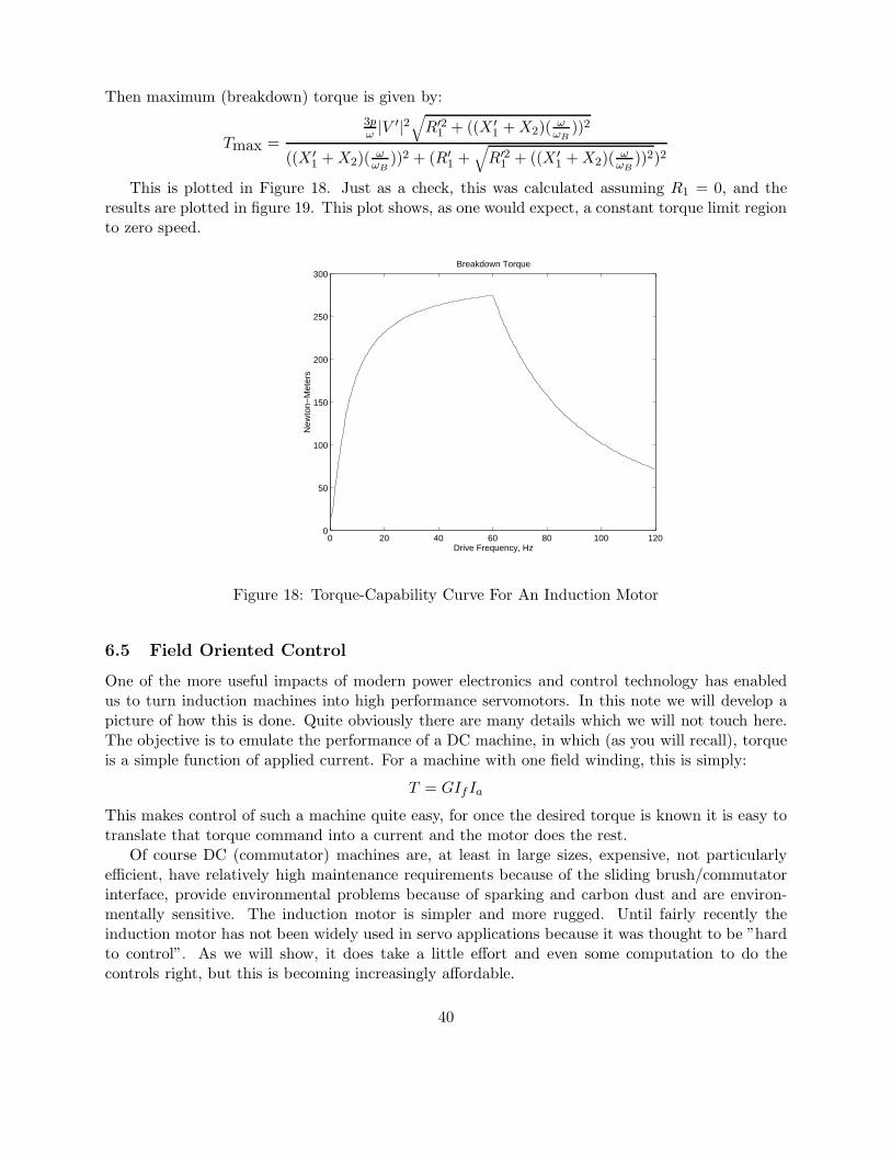
Then maximum (breakdown) torque is given by:

3p |V ′|2√

R′2 X2)(ω

1 + ((X ′1 + ))2

ω ωTmax =

B

((X ′1 +X2)(

ω ))2 + (R′1 + R′2

1 + ((X ′ + ω

B 1 X2)( ))2)2ω ωB

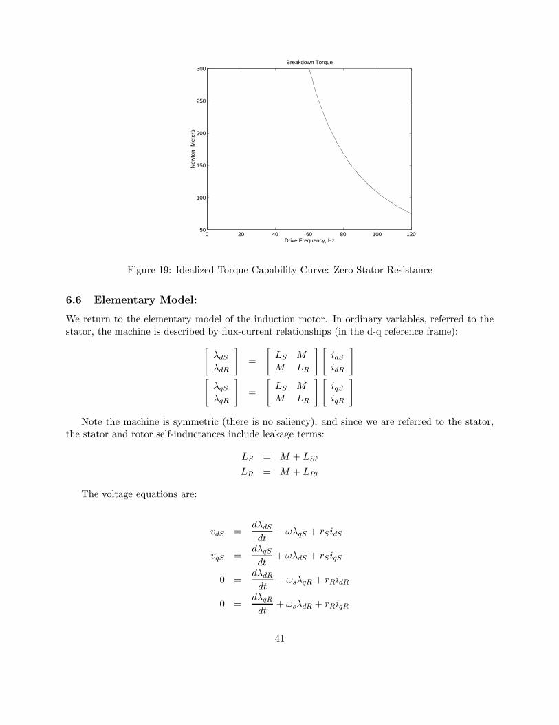
This is plotted in Figure 18. Just as a check, th

√

is was calculated assuming R1 = 0, and theresults are plotted in figure 19. This plot shows, as one would expect, a constant torque limit regionto zero speed.

0 20 40 60 80 100 1200

50

100

150

200

250

300Breakdown Torque

New

ton−

Met

ers

Drive Frequency, Hz

Figure 18: Torque-Capability Curve For An Induction Motor

6.5 Field Oriented Control

One of the more useful impacts of modern power electronics and control technology has enabledus to turn induction machines into high performance servomotors. In this note we will develop apicture of how this is done. Quite obviously there are many details which we will not touch here.The objective is to emulate the performance of a DC machine, in which (as you will recall), torqueis a simple function of applied current. For a machine with one field winding, this is simply:

T = GIf Ia

This makes control of such a machine quite easy, for once the desired torque is known it is easy totranslate that torque command into a current and the motor does the rest.

Of course DC (commutator) machines are, at least in large sizes, expensive, not particularlyefficient, have relatively high maintenance requirements because of the sliding brush/commutatorinterface, provide environmental problems because of sparking and carbon dust and are environ-mentally sensitive. The induction motor is simpler and more rugged. Until fairly recently theinduction motor has not been widely used in servo applications because it was thought to be ”hardto control”. As we will show, it does take a little effort and even some computation to do thecontrols right, but this is becoming increasingly affordable.

40

0 20 40 60 80 100 12050

100

150

200

250

300Breakdown Torque

New

ton−

Met

ers

Drive Frequency, Hz

Figure 19: Idealized Torque Capability Curve: Zero Stator Resistance

6.6 Elementary Model:

We return to the elementary model of the induction motor. In ordinary variables, referred to thestator, the machine is described by flux-current relationships (in the d-q reference frame):

[

λdS

λdR

]

=

[

LS M idS

M LR

] [

idR

]

[

λqS

λqR

]

L=

[

S MM LR

] [

iqS

iqR

]

Note the machine is symmetric (there is no saliency), and since we are referred to the stator,the stator and rotor self-inductances include leakage terms:

LS = M + LSℓ

LR = M + LRℓ

The voltage equations are:

dλdSvdS = − ωλqS + rSidS

dtdλqS

vqS = + ωλdS + rSiqSdtdλdR

0 = − ωsλqR + rRidRdtdλqR

0 = + ωsλdR + rRiqRdt

41

Note that both rotor and stator have “speed” voltage terms since they are both rotating withrespect to the rotating coordinate system. The speed of the rotating coordinate system is w withrespect to the stator. With respect to the rotor that speed is , where wm is the rotor mechanicalspeed. Note that this analysis does not require that the reference frame coordinate system speedw be constant.

Torque is given by:

T e 3= p (λdSiqS − λqSidS)

2

6.7 Simulation Model

As a first step in developing a simulation model, see that the inversion of the flux-current relation-ship is (we use the d- axis since the q- axis is identical):

LR MidS = λ

LSLR − dSM2

− λLSLR − dR

M2

M LidR = λ

LSLR − dSM2

− SλdR

LSL − 2R M

Now, if we make the following definitions (the motivation for this should by now be obvious):

Xd = ω0LS

Xkd = ω0LR

Xad = ω0M

X ′M2

d = ω0

(

LS −LR

)

the currents become:

ω0 Xad ω0idS =

X ′λdS ′

λdRd

−Xkd Xd

Xad ω0 Xd ω0idR =

′λdS λ

Xk Xd

−X ′ dR

d d Xkd

The q- axis is the same.Torque may be, with these calculations for current, written as:

3 3 ωTe = p (λdSiqS − 0Xad

λqSidS) = − p′(λdSλqR

2 2 XkdXd

− λqSλdR)

Note that the usual problems with ordinary variables hold here: the foregoing expression waswritten assuming the variables are expressed as peak quantities. If RMS is used we must replace3/2 by 3!

With these, the simulation model is quite straightforward. The state equations are:

dλdS= VdS + ωλqS

dt−RSidS

dλqS= VqS − ωλdS

dt−RSiqS

42

dλdR= ωsλqR

dt−RRidR

dλqR= −ωsλdR −RSiqR

dtdΩm 1

= (Te + Tm)dt J

where the rotor frequency (slip frequency) is:

ωs = ω − pΩm

For simple simulations and constant excitaion frequency, the choice of coordinate systems isarbitrary, so we can choose something convenient. For example, we might choose to fix the coordi-nate system to a synchronously rotating frame, so that stator frequency ω = ω0. In this case, wecould pick the stator voltage to lie on one axis or another. A common choice is Vd = 0 and Vq = V .

6.8 Control Model

If we are going to turn the machine into a servomotor, we will want to be a bit more sophisticatedabout our coordinate system. In general, the principle of field-oriented control is much like emu-lating the function of a DC (commutator) machine. We figure out where the flux is, then injectcurrent to interact most directly with the flux.

As a first step, note that because the two stator flux linkages are the sum of air-gap and leakageflux,

λdS = λagd + LSℓidS

λqS = λagq + LSℓiqS

This means that we can re-write torque as:

T e 3= p (λagdiqS

2− λagqidS)

Next, note that the rotor flux is, similarly, related to air-gap flux:

λagd = λdR − LRℓidR

λagq = λqR − LRℓiqR

Torque now becomes:

3 3T e = p (λdRiqS − λqRidS) − pLRℓ (idRiqS i

2 2− qRidS)

Now, since the rotor currents could be written as:

λdR MidR =

LR− idSLR

λqR MiqR =

LR

− iqSLR

43

That second term can be written as:

1idRiqS − iqRidS = (λdRiqS

LR− λqRidS)

So that torque is now:

e 3(

LRℓ 3 MT = p 1 − (λdRiqS λqRidS) = p (λdRiqS λqRidS)

2 LR

)

−2 LR

−

6.9 Field-Oriented Strategy:

What is done in field-oriented control is to establish a rotor flux in a known position (usually thisposition is the d- axis of the transformation) and then put a current on the orthogonal axis (whereit will be most effective in producing torque). That is, we will attempt to set

λdR = Λ0

λqR = 0

Then torque is produced by applying quadrature-axis current:

e 3 MT = p Λ0iqS

2 LR

The process is almost that simple. There are a few details involved in figuring out where thequadrature axis is and how hard to drive the direct axis (magnetizing) current.

Now, suppose we can succeed in putting flux on the right axis, so that λqR = 0, then the tworotor voltage equations are:

dλdR0 =

dt− ωsλqR + rRIdR

dλqR0 = + ωsλdR + rRIqR

dt

Now, since the rotor currents are:

λdR MidR = − idS

LR LR

λqR MiqR =

LR

− iqSLR

The voltage expressions become, accounting for the fact that there is no rotor quadrature axisflux:

dλdR λdR M0 = + rR idS

dt

(

LR−LR

)

M0 = ωsλdR − rR iqS

LR

Noting that the rotor time constant is

LRTR =

rR

44

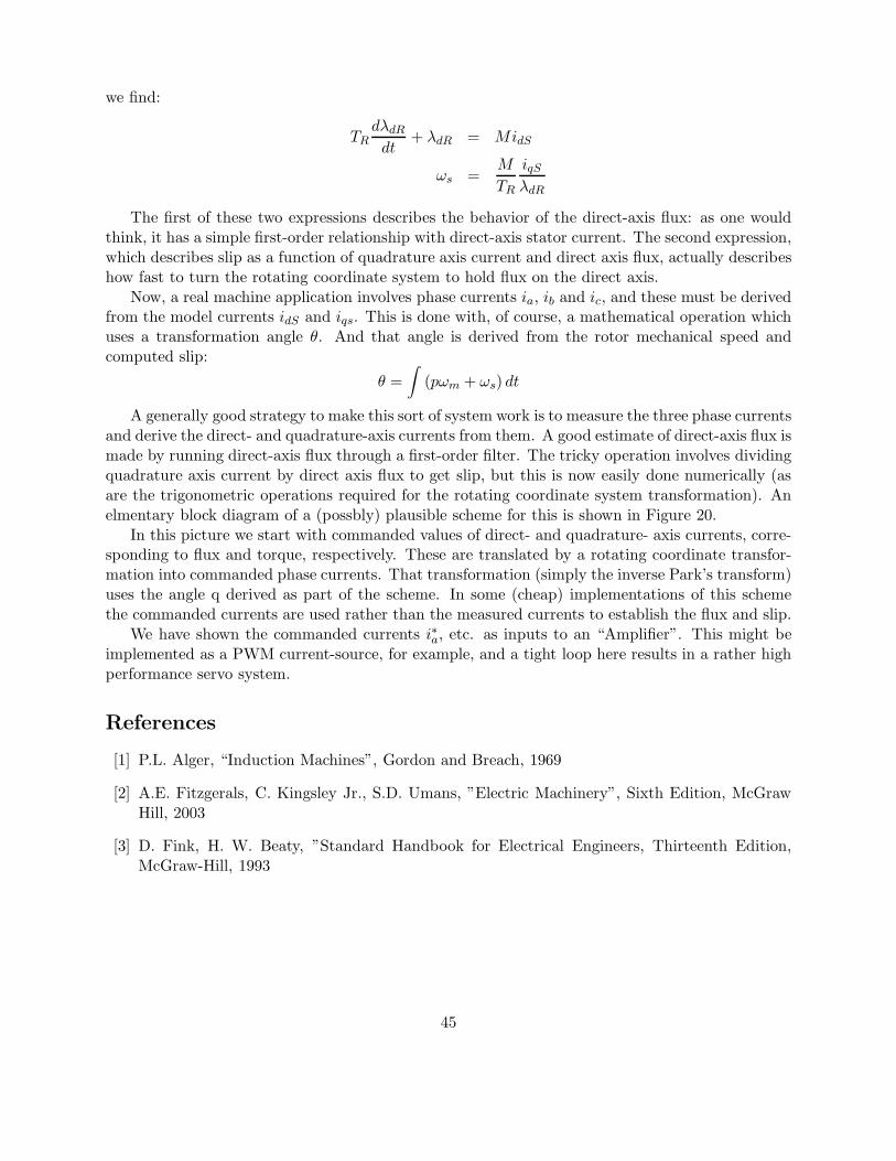
we find:

dλdRTR + λdR = MidS

dtM iqS

ωs =TR λdR

The first of these two expressions describes the behavior of the direct-axis flux: as one wouldthink, it has a simple first-order relationship with direct-axis stator current. The second expression,which describes slip as a function of quadrature axis current and direct axis flux, actually describeshow fast to turn the rotating coordinate system to hold flux on the direct axis.

Now, a real machine application involves phase currents ia, ib and ic, and these must be derivedfrom the model currents idS and iqs. This is done with, of course, a mathematical operation whichuses a transformation angle θ. And that angle is derived from the rotor mechanical speed andcomputed slip:

θ =

∫

(pωm + ωs) dt

A generally good strategy to make this sort of system work is to measure the three phase currentsand derive the direct- and quadrature-axis currents from them. A good estimate of direct-axis flux ismade by running direct-axis flux through a first-order filter. The tricky operation involves dividingquadrature axis current by direct axis flux to get slip, but this is now easily done numerically (asare the trigonometric operations required for the rotating coordinate system transformation). Anelmentary block diagram of a (possbly) plausible scheme for this is shown in Figure 20.

In this picture we start with commanded values of direct- and quadrature- axis currents, corre-sponding to flux and torque, respectively. These are translated by a rotating coordinate transfor-mation into commanded phase currents. That transformation (simply the inverse Park’s transform)uses the angle q derived as part of the scheme. In some (cheap) implementations of this schemethe commanded currents are used rather than the measured currents to establish the flux and slip.

We have shown the commanded currents i∗a, etc. as inputs to an “Amplifier”. This might beimplemented as a PWM current-source, for example, and a tight loop here results in a rather highperformance servo system.

References

[1] P.L. Alger, “Induction Machines”, Gordon and Breach, 1969

[2] A.E. Fitzgerals, C. Kingsley Jr., S.D. Umans, ”Electric Machinery”, Sixth Edition, McGrawHill, 2003

[3] D. Fink, H. W. Beaty, ”Standard Handbook for Electrical Engineers, Thirteenth Edition,McGraw-Hill, 1993

45

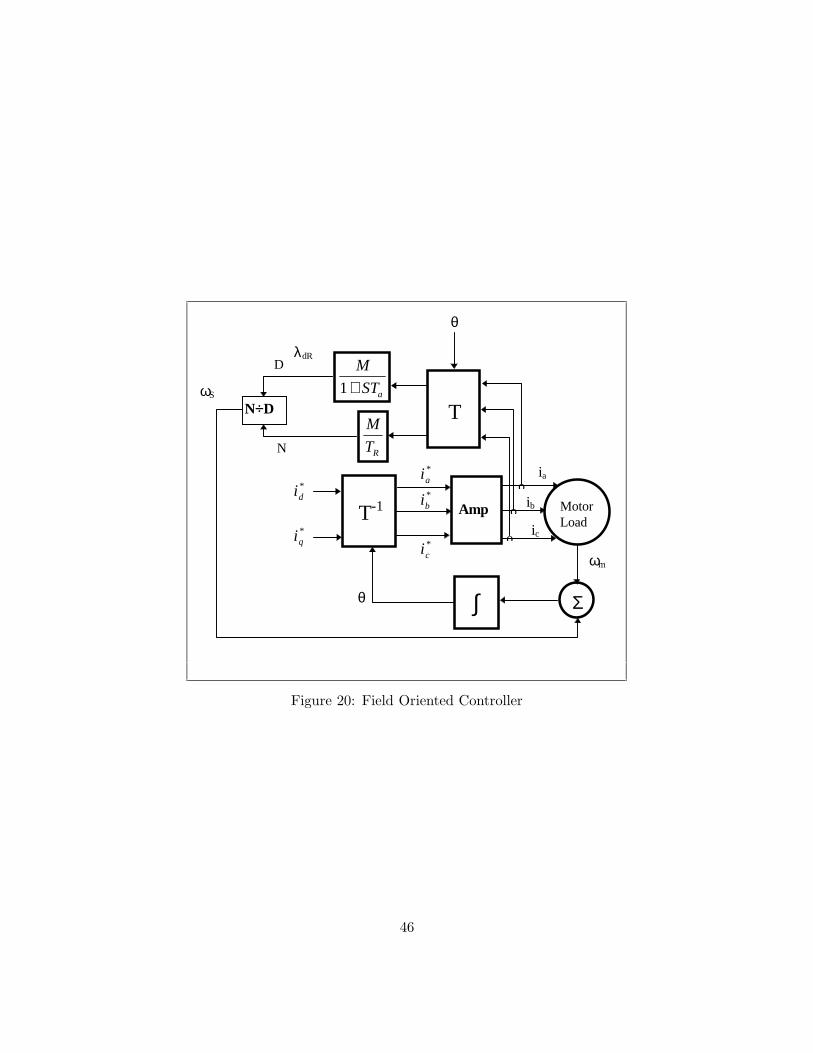
MotorLoad

ic

ib

ia

Amp

o

o

o

T-1

T

iq*

id*

ic*

ib*

ia*

M

STa1+

M

TR

N÷÷D

N

D

Σ

ωm

ωS

∫

θ

θ

λdR

Figure 20: Field Oriented Controller

46

r1 x1∧ ∧ ∧∨ ∨

∩∩∩∩⊃⊃⊃jx2s

⊃<

⊃>

⊃jx2c⊃⊃⊃jxag < rc

⊃>

⊃⊃⊃xc

⊃⊃ < ⊃ < <

> r2s > r2< < c

> s > s< <

⊃jx

⊃⊃ ⊃⊃ 2s5 ⊃jx2c5⊃ ⊃ ⊃⊃⊃jxa5⊃ < <

> r2s5 > r2c5< <> s5 > s5< <

⊃jx2s7

⊃⊃ ⊃⊃ ⊃jx2c7⊃ ⊃⊃jxa7

⊃⊃⊃ < <

> r2s7 > r2c7< <> s7 > s7

< <

⊃m

⊃⊃ ⊃⊃jx2s ⊃jx2cm⊃⊃⊃jxam

⊃ ⊃⊃ < <

> r2sm > r2cm< <> sm > sm

< <

⊃⊃⊃jx2sp

⊃⊃⊃jx2cp

⊃xap

⊃ ⊃⊃⊃j⊃ < <r> 2sp r> 2cp< <> sp > sp

< <

Figure 21: Extended Equivalent Circuit

47

MIT OpenCourseWarehttp://ocw.mit.edu

6.685 Electric MachinesFall 2013

For information about citing these materials or our Terms of Use, visit: http://ocw.mit.edu/terms.