Massachusetts Institute of Technology Department of ...ihler/papers/proposal.pdfDepartment of...
71
Massachusetts Institute of Technology Department of Electrical Engineering and Computer Science Proposal for Thesis Research in Partial Fulfillment of the Requirements for the Degree of Doctor of Philosophy Title: Nonparametric representations for inference in networks of sensors Submitted by: Alexander T. Ihler 77 Massachusetts Avenue Room 35-425 Cambridge, MA 02139 (Signature of Author) Date of Submission: September 2003 Expected Date of Completion: June 2005 Laboratory: Laboratory for Information and Decision Systems Brief Statement of the Problem: Improvements in sensing technology and wireless communications are rapidly increasing the importance of sensor networks as a signal processing application. The growing availability of tiny, inexpensive cameras, microphones, and other sensors has begun to make practical the creation of ubiquitous networks of sensors. These networks receive tremendous amounts of data, which must be fused to extract relevant information about the environment. In many collaborative sensing problems, strong assumptions and prior models on the joint distributions between signals are used to make the problem more tractable. However, there are a number of situations in which we lack prior knowledge of these distributions. When this is the case, we must find ways to determine the structure and relationships within the data. This may include modeling the dynamic structure of signals, determining which signals are co-dependent, and modeling their joint relationships. This thesis will focus on nonparametric representations, in particular kernel density estimates. Kernel methods can be used to model a wide variety of distributions; however, they often become computationally intractable for large problems. The goal of this thesis is to apply nonparametric models to inference in sensor networks, and to find ways to make these techniques computationally tractable.
Transcript of Massachusetts Institute of Technology Department of ...ihler/papers/proposal.pdfDepartment of...

Massachusetts Institute of Technology
Department of Electrical Engineering
and Computer Science
Proposal for Thesis Research in Partial Fulfillment
of the Requirements for the Degree of
Doctor of Philosophy
Title: Nonparametric representations for inference in networks of sensorsSubmitted by: Alexander T. Ihler
77 Massachusetts AvenueRoom 35-425Cambridge, MA 02139
(Signature of Author)
Date of Submission: September 2003Expected Date of Completion: June 2005
Laboratory: Laboratory for Information and Decision Systems
Brief Statement of the Problem:
Improvements in sensing technology and wireless communications are rapidly increasing theimportance of sensor networks as a signal processing application. The growing availability of tiny,inexpensive cameras, microphones, and other sensors has begun to make practical the creation ofubiquitous networks of sensors. These networks receive tremendous amounts of data, which mustbe fused to extract relevant information about the environment. In many collaborative sensingproblems, strong assumptions and prior models on the joint distributions between signals are usedto make the problem more tractable. However, there are a number of situations in which we lackprior knowledge of these distributions. When this is the case, we must find ways to determine thestructure and relationships within the data. This may include modeling the dynamic structure ofsignals, determining which signals are co-dependent, and modeling their joint relationships.
This thesis will focus on nonparametric representations, in particular kernel density estimates.Kernel methods can be used to model a wide variety of distributions; however, they often becomecomputationally intractable for large problems. The goal of this thesis is to apply nonparametricmodels to inference in sensor networks, and to find ways to make these techniques computationallytractable.

Massachusetts Institute of TechnologyDepartment of Electrical Engineering
and Computer ScienceCambridge, Massachusetts 02139
Doctoral Thesis Supervision Agreement
To: Department Graduate CommitteeFrom: Professor Alan S. Willsky
The program outlined in the proposal:
Title: Nonparametric representations for inference in networks of sensorsAuthor: Alexander T. Ihler
Date: September 2003
is adequate for a Doctoral thesis. I believe that appropriate readers for this thesis would be:
Reader 1: Professor Sanjeev R. KulkarniReader 2: Professor William T. Freeman
Facilities and support for the research outlined in the proposal are available. I am willing tosupervise the thesis jointly with Dr. John W. Fisher and evaluate the thesis report.
Signed:Professor of Electrical Engineering
and Computer Science
Date:
Comments:

Massachusetts Institute of TechnologyDepartment of Electrical Engineering
and Computer ScienceCambridge, Massachusetts 02139
Doctoral Thesis Supervision Agreement
To: Department Graduate CommitteeFrom: Dr. John W. Fisher
The program outlined in the proposal:
Title: Nonparametric representations for inference in networks of sensorsAuthor: Alexander T. Ihler
Date: September 2003
is adequate for a Doctoral thesis. I believe that appropriate readers for this thesis would be:
Reader 1: Professor Sanjeev R. KulkarniReader 2: Professor William T. Freeman
Facilities and support for the research outlined in the proposal are available. I am willing tosupervise the thesis jointly with Professor Alan S. Willsky and evaluate the thesis report.
Signed:Principal Research Scientist
AI Lab, EECS
Date:
Comments:

Massachusetts Institute of TechnologyDepartment of Electrical Engineering
and Computer ScienceCambridge, Massachusetts 02139
Doctoral Thesis Reader Agreement
To: Department Graduate CommitteeFrom: Professor Sanjeev R. Kulkarni
The program outlined in the proposal:
Title: Nonparametric representations for inference in networks of sensorsAuthor: Alexander T. Ihler
Date: September 2003Supervisors: Professor Alan S. Willsky
Dr. John W. FisherOther Readers: Professor William T. Freeman
is adequate for a Doctoral thesis. I am willing to aid in guiding the research and in evaluating thethesis report as a reader.
Signed:Associate Professor of Electrical Engineering
Princeton University
Date:
Comments:

Massachusetts Institute of TechnologyDepartment of Electrical Engineering
and Computer ScienceCambridge, Massachusetts 02139
Doctoral Thesis Reader Agreement
To: Department Graduate CommitteeFrom: Professor William T. Freeman
The program outlined in the proposal:
Title: Nonparametric representations for inference in networks of sensorsAuthor: Alexander T. Ihler
Date: September 2003Supervisors: Professor Alan S. Willsky
Dr. John W. FisherOther Readers: Professor Sanjeev R. Kulkarni
is adequate for a Doctoral thesis. I am willing to aid in guiding the research and in evaluating thethesis report as a reader.
Signed:Associate Professor of Electrical Engineering
and Computer Science
Date:
Comments:


CONTENTS i
Contents
List of Figures iii
List of Tables iii
1 Introduction 11.1 A canonical example in data association . . . . . . . . . . . . . . . . . . . . . . . . . 21.2 Goals . . . . . . . . . . . . . . . . . . . . . . . . . . . . . . . . . . . . . . . . . . . . 5
2 Informative Subspaces 52.1 Dynamical Systems . . . . . . . . . . . . . . . . . . . . . . . . . . . . . . . . . . . . . 5
2.1.1 Background . . . . . . . . . . . . . . . . . . . . . . . . . . . . . . . . . . . . . 62.1.2 Nonparametric Estimation of Dynamics . . . . . . . . . . . . . . . . . . . . . 62.1.3 Signature Dynamics . . . . . . . . . . . . . . . . . . . . . . . . . . . . . . . . 7
2.2 Data Association Across Nonlinear & Dispersive Media . . . . . . . . . . . . . . . . 82.2.1 Data Association as a Hypothesis Test . . . . . . . . . . . . . . . . . . . . . . 82.2.2 Features for Hypothesis Testing . . . . . . . . . . . . . . . . . . . . . . . . . . 102.2.3 Data Association Examples . . . . . . . . . . . . . . . . . . . . . . . . . . . . 12
2.3 Learning Informative Subspaces . . . . . . . . . . . . . . . . . . . . . . . . . . . . . . 132.3.1 Estimating Mutual Information . . . . . . . . . . . . . . . . . . . . . . . . . . 132.3.2 Statistic Form . . . . . . . . . . . . . . . . . . . . . . . . . . . . . . . . . . . 14
3 Graphical Models for Sensor Networks 143.1 Graph Structures . . . . . . . . . . . . . . . . . . . . . . . . . . . . . . . . . . . . . . 143.2 Graphical Models . . . . . . . . . . . . . . . . . . . . . . . . . . . . . . . . . . . . . . 153.3 Inference Algorithms on Graphs . . . . . . . . . . . . . . . . . . . . . . . . . . . . . . 17
3.3.1 Belief Propagation . . . . . . . . . . . . . . . . . . . . . . . . . . . . . . . . . 173.3.2 Particle Filtering . . . . . . . . . . . . . . . . . . . . . . . . . . . . . . . . . . 183.3.3 Nonparametric Belief Propagation . . . . . . . . . . . . . . . . . . . . . . . . 18
3.4 Application to Sensor Networks . . . . . . . . . . . . . . . . . . . . . . . . . . . . . . 183.4.1 Graph Structure . . . . . . . . . . . . . . . . . . . . . . . . . . . . . . . . . . 193.4.2 Representing Messages and Belief . . . . . . . . . . . . . . . . . . . . . . . . . 203.4.3 Continuing efforts . . . . . . . . . . . . . . . . . . . . . . . . . . . . . . . . . 22
4 Proposed Research 234.1 Source Separation . . . . . . . . . . . . . . . . . . . . . . . . . . . . . . . . . . . . . 244.2 Learning Graph Structure . . . . . . . . . . . . . . . . . . . . . . . . . . . . . . . . . 25
4.2.1 Connectivity . . . . . . . . . . . . . . . . . . . . . . . . . . . . . . . . . . . . 254.2.2 Graph interrelations . . . . . . . . . . . . . . . . . . . . . . . . . . . . . . . . 26
4.3 Decentralized Data Processing . . . . . . . . . . . . . . . . . . . . . . . . . . . . . . 274.4 Timeline . . . . . . . . . . . . . . . . . . . . . . . . . . . . . . . . . . . . . . . . . . . 274.5 Conclusions . . . . . . . . . . . . . . . . . . . . . . . . . . . . . . . . . . . . . . . . . 28
A Information Theory 29
B Nonparametric Density Estimation 29B.1 Kernel density estimates . . . . . . . . . . . . . . . . . . . . . . . . . . . . . . . . . . 30B.2 Estimating information-theoretic quantities . . . . . . . . . . . . . . . . . . . . . . . 31

ii CONTENTS
C Nonparametric Belief Propagation 32C.1 Introduction . . . . . . . . . . . . . . . . . . . . . . . . . . . . . . . . . . . . . . . . . 32C.2 Undirected Graphical Models . . . . . . . . . . . . . . . . . . . . . . . . . . . . . . . 34
C.2.1 Belief Propagation . . . . . . . . . . . . . . . . . . . . . . . . . . . . . . . . . 35C.2.2 Nonparametric Representations . . . . . . . . . . . . . . . . . . . . . . . . . . 35
C.3 Nonparametric Message Updates . . . . . . . . . . . . . . . . . . . . . . . . . . . . . 36C.3.1 Message Products . . . . . . . . . . . . . . . . . . . . . . . . . . . . . . . . . 36C.3.2 Message Propagation . . . . . . . . . . . . . . . . . . . . . . . . . . . . . . . . 39
C.4 Gaussian Graphical Models . . . . . . . . . . . . . . . . . . . . . . . . . . . . . . . . 40C.5 Component–Based Face Models . . . . . . . . . . . . . . . . . . . . . . . . . . . . . . 41
C.5.1 Model Construction . . . . . . . . . . . . . . . . . . . . . . . . . . . . . . . . 41C.5.2 Estimation of Occluded Features . . . . . . . . . . . . . . . . . . . . . . . . . 43
C.6 Discussion . . . . . . . . . . . . . . . . . . . . . . . . . . . . . . . . . . . . . . . . . . 44
D Hypothesis Testing over Factorizations for Data Association 44D.1 Introduction . . . . . . . . . . . . . . . . . . . . . . . . . . . . . . . . . . . . . . . . . 44D.2 An Information-Theoretic Interpretation of Data Association . . . . . . . . . . . . . 46
D.2.1 Mutual Information . . . . . . . . . . . . . . . . . . . . . . . . . . . . . . . . 46D.2.2 Data Association as a Hypothesis Test . . . . . . . . . . . . . . . . . . . . . . 47
D.3 Algorithmic Details . . . . . . . . . . . . . . . . . . . . . . . . . . . . . . . . . . . . . 50D.3.1 Estimating Mutual Information . . . . . . . . . . . . . . . . . . . . . . . . . . 51D.3.2 Learning Sufficient Statistics . . . . . . . . . . . . . . . . . . . . . . . . . . . 52
D.4 Data Association of Two Sources . . . . . . . . . . . . . . . . . . . . . . . . . . . . . 52D.5 Extension to Many Sources . . . . . . . . . . . . . . . . . . . . . . . . . . . . . . . . 54D.6 Discussion . . . . . . . . . . . . . . . . . . . . . . . . . . . . . . . . . . . . . . . . . . 56

LIST OF FIGURES iii
List of Figures
1 The data association problem . . . . . . . . . . . . . . . . . . . . . . . . . . . . . . . 22 Capturing the time dynamics of a signature . . . . . . . . . . . . . . . . . . . . . . . 83 The data association problem . . . . . . . . . . . . . . . . . . . . . . . . . . . . . . . 84 Data association across a nonlinear phase all-pass filter . . . . . . . . . . . . . . . . . 125 Associating non-overlapping harmonic spectra . . . . . . . . . . . . . . . . . . . . . . 136 Graph separation and grouping variables . . . . . . . . . . . . . . . . . . . . . . . . . 167 N sensors distributed uniformly within radius R0 (light gray), with each sensor seeing its
neighbors within radius R1 (dark gray). . . . . . . . . . . . . . . . . . . . . . . . . . . . 198 Probability of satisfying the uniqueness condition for various N , as a function of R1/R0;
inclusion of the constraints due to non-observation shifts the curves leftward by about 10%
(shown as dashed lines) . . . . . . . . . . . . . . . . . . . . . . . . . . . . . . . . . . . 2010 (a) A small (12-sensor) graph and the observable pairwise distances; sensors with prior
information of location (a minimal set) are shown in green. A centralized estimate of the
MAP solution (b) shows similar residual error (red) to NBP’s approximate (marginal MAP)
solution (c). . . . . . . . . . . . . . . . . . . . . . . . . . . . . . . . . . . . . . . . . . 219 Uncertainty in a sensor’s location given the position of one neighbor appears as ring, rep-
resented nonparametrically with many samples. Here, four sensors collaborate to find the
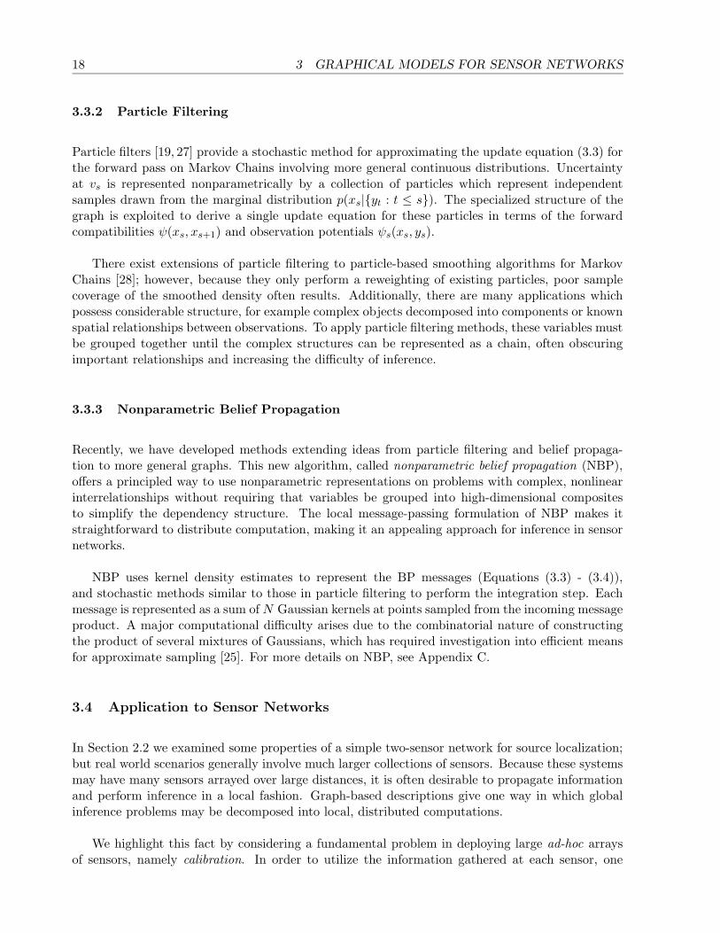
location of their neighbor and its estimated uncertainty (shown in blue). . . . . . . . . . . 2111 (a) A large (100-sensor) graph and the observable pairwise distances; although a naive NBP
solution (b) is caught in a local maximum (many points find reflected versions of their true
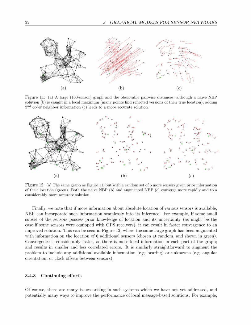
location), adding 2nd order neighbor information (c) leads to a more accurate solution. . . . 2212 (a) The same graph as Figure 11, but with a random set of 6 more sensors given prior
information of their location (green). Both the naive NBP (b) and augmented NBP (c)
converge more rapidly and to a considerably more accurate solution. . . . . . . . . . . . . 2213 Kernel size choice . . . . . . . . . . . . . . . . . . . . . . . . . . . . . . . . . . . . . . 3014 Graphical Models . . . . . . . . . . . . . . . . . . . . . . . . . . . . . . . . . . . . . . 3315 NBP Gibbs Sampler . . . . . . . . . . . . . . . . . . . . . . . . . . . . . . . . . . . . 3716 NBP on jointly Gaussian models . . . . . . . . . . . . . . . . . . . . . . . . . . . . . 4117 AR Face Database . . . . . . . . . . . . . . . . . . . . . . . . . . . . . . . . . . . . . 4218 PCA-based facial component model . . . . . . . . . . . . . . . . . . . . . . . . . . . 4219 Empirical joint densities of PCA coefficients . . . . . . . . . . . . . . . . . . . . . . . 4220 NBP estimation of occluded mouth . . . . . . . . . . . . . . . . . . . . . . . . . . . . 4521 NBP estimation of occluded eye . . . . . . . . . . . . . . . . . . . . . . . . . . . . . . 4522 The data association problem . . . . . . . . . . . . . . . . . . . . . . . . . . . . . . . 4723 Uncorrelated but dependent variables . . . . . . . . . . . . . . . . . . . . . . . . . . 4724 Data association across a nonlinear phase all-pass filter . . . . . . . . . . . . . . . . . 5325 Associating non-overlapping harmonic spectra . . . . . . . . . . . . . . . . . . . . . . 5426 Associating non-overlapping wideband harmonic spectra . . . . . . . . . . . . . . . . 5427 Association between many signal pairs . . . . . . . . . . . . . . . . . . . . . . . . . . 5728 Statistics learned on concatenated signals and their L1 norm . . . . . . . . . . . . . 57
List of Tables


1
1 Introduction
Signal processing in networks of sensors and statistical inference in graphical models are two re-lated problems with broad application. Both have been primarily studied under strong modelingassumptions and considerable prior knowledge. For example, signal processing in sensor networkshas focused on optimal estimation using strong prior models, while work in graphical models hasprogressed in both exact and approximate methods on fully specified graphs. This proposal seeksto address aspects of both problems in which some of the restrictive assumptions are relaxed.
The problem of inference (e.g. localization, tracking, or classification of objects of interest) innetworks of sensors is of growing importance with a wide variety of applications ranging from mili-tary battlefield awareness to civilian security and smart buildings. The idea of pervasive sensing is acompelling one – inexpensive sensors blanketing a region and reporting everything within. In sucha scenario, there might be thousands of sensors, consisting of many different sensing modalities(CCD cameras, acoustic or seismic microphones, infrared range-finders, and more). Inference iscomplicated by the fact that we may have only rough calibration information, if any – for examplewe may be uncertain about sensors’ locations and directional responses. Furthermore, there maybe unknown or complex relationships among signals measured by the sensors – perspective changes,medium-dependent changes in a signal’s phase and magnitude, and the presence of noise or inten-tional jamming signals. Finally, centralized data processing may be impractical due to constraintson transmission power and battery life.
Inference in networks of sensors in situations like those described above is a formidable problem.A few of the important issues which make it challenging include data fusion, not just in situationswith well-modeled interactions but also in cases involving complex interrelations, e.g. between dif-ferent sensor types; robustness to uncertainty in uncalibrated sensors, efficiency in communications,and finally scalability to large numbers of sensors within a network. In particular, it is often thecase that as methods gain robustness to complex interactions and uncertainty, they begin to loseefficiency and scalability. When examining these problems, we must take care to do so withoutlosing sight of computational and communication concerns.
The goal of this thesis is to apply nonparametric methods to address the issues above, allowingapplication to problems where we do not have access to prior models. We begin with a simple mo-tivating example in data association, to illustrate some of the issues which arise when we substitutenonparametric methods for strong modeling assumptions. This is followed by a brief discussionof the goals and direction of the thesis. In the subsequent two sections we describe some relevantbackground material and preliminary research. Section 2 presents our prior work in information-maximizing subspace projections for inference, including a more in-depth discussion of the dataassociation problem surveyed in Section 1.1. In Section 3 we describe sensor networks using agraphical model framework, and discuss the application of nonparametric methods to inference onsuch models. We conclude with Section 4, which summarizes and discusses directions for researchto be explored in this thesis, along with a timeline for completion.
Throughout this proposal, we shall take the term sensor to mean one or several approximatelyco-located data acquisition elements, whether of the same or different modality, and network toindicate a collection of such sensors.

2 1 INTRODUCTION
����������� ��������� ���
��
�����
���
Figure 1: The data association problem: two pairs of measurements results in estimated targets ateither the circles or the squares; but which remains ambiguous.
1.1 A canonical example in data association
Consider the following fairly simple example problem, which illustrates a single element of theuncertainty found in traditional tracking problems. Suppose we have a pair of widely spacedacoustic sensors, where each sensor is a small array of many elements. Each sensor produces onlybearing information, which in itself is insufficient to localize the source. However, triangulation ofbearing measurements from multiple sensors can be used to estimate the target location. For asingle target, a pair of sensors is sufficient to perform this triangulation.
However, complications arise when there are multiple targets within a pair of sensors’ fieldsof view. Each sensor determines two bearings; but this yields four possible locations for only twotargets, as depicted in Figure 1. With only bearing information, there is no way to know whichone of these target pairs is real, and which is the artifact.
One way to resolve this ambiguity is through data association, determining which receivedsignal at A corresponds to a given one at B. We can extract directional estimates of each sourceindividually, and if we possessed a model for the relationship between the observed signals undereach of the two hypotheses
H1 : A1 ↔ B1, A2 ↔ B2 (1.1)
H2 : A1 ↔ B2, A2 ↔ B1
the optimal correspondence decision given N independent observations takes the form of a test onthe mean of the log-likelihood ratio:
1
NlogL =
1
N
N∑
k=1
logpH1
([A1, A2, B1, B2]k)
pH2([A1, A2, B1, B2]k)
H1≥<H2
γ (1.2)
where pHi(·) is the joint distribution of the source signals under hypothesis i, and the constant γ is
determined by the prior probabilities of the Hi and the desired probabilities of incorrect decisions.Unfortunately, for a variety of reasons we may not know the joint distributions in Equation (1.2).For example, even given a model of the sources, differences in phase and group delay due toinhomogenous media create changes in the magnitude and time of arrival between frequencies inthe observations, sometimes referred to as signal incoherence. Constructing a complete model

1.1 A canonical example in data association 3
of these distributions is equivalent to solving a source reconstruction problem, a complex inverseproblem which may be ill-posed. In contrast, we expect the binary association between thesevariables to be easier to determine. We therefore seek methods which do not require solving thefull inverse problem, but rather focus on determining the association.
Without any restrictions on the joint relationships pH1and pH2
, the problem is ill-posed. There-fore we add a mild assumption, that the two sources are statistically independent, and treat theactual probability densities as unknown nuisance parameters. This is sufficient to derive a meansof testing the density factorization implied by hypothesis Hi directly, without making assumptionsabout the form of the densities.
A detailed analysis of this problem is presented in Section 2.2; however, for illustration purposeswe highlight some of the results here. If we construct density estimates using some or all of thedata to be tested, and impose the independence constraint of Hi, we can reformulate the test asone between factorizations of the density estimate, specifically between the two hypotheses
H1 : p(A1, B1, A2, B2) = pH1(A1, B1, A2, B2) = pH1
(A1, B1)pH1(A2, B2)
H2 : p(A1, B1, A2, B2) = pH2(A1, B1, A2, B2) = pH2
(A1, B2)pH2(A2, B1) (1.3)
where pHidenotes an estimate of the density which factors as shown.
To provide some initial analysis and insight into this problem, we make one assumption: thatthe estimates of the probability distributions pH1
, pH2are consistent – i.e. that these estimates
converge to their true values as the number, N , of available data samples grows. In our algorithmswe ensure that this assumption is satisfied by using nonparametric (kernel-based) methods, whichare consistent for a wide class of distributions; a brief overview of kernel methods is given inAppendix B. Assuming consistency, and denoting the likelihood ratio of these estimates by L, the(normalized) log likelihood ratio and its large data limit are given by
1
Nlog L =
1
N
N∑
k=1
logpH1
([A1, A2, B1, B2]k)
pH2([A1, A2, B1, B2]k)
→ I(A1;B1) + I(A2;B2)− I(A1;B2)− I(A2;B1) as N →∞ (1.4)
where I is the mutual information (MI) between the two arguments. More detail on such information-theoretic quantities can be found in Appendix A.
Of course, the values of the MI quantities in Equation (1.4) depend on which hypothesis istrue. For example, if H1 is true, we know from Equation (1.3) that I(A1;B2) and I(A2;B1) arezero (with the other two terms being zero instead if H2 is true). Thus, if we could compute theseinformation-theoretic quantities exactly, we would simply compare the quantity in the second lineof Equation (1.4) with zero to decide between the hypotheses.
In reality, we do not have infinite amounts of data. In this case neither will the probabilitydensities pH1
, pH2have converged nor will the normalized likelihood ratio have converged to its
(deterministic) large data limit. Moreover, in many problems the likelihood ratio L may be toodifficult to compute directly. These issues lead us to consider a test based on direct estimates(denoted by I) of the various MI quantities in Equation (1.4), using a threshold (possibly different

4 1 INTRODUCTION
from zero), as the decision boundary:
I(A1;B1) + I(A2;B2)− I(A1;B2)− I(A2;B1)
H1≥<H2
γ (1.5)
In particular, for the applications of interest to us the observations have high dimension (forexample video imagery or Fourier spectra). Unfortunately, adequate estimation of high-dimensionaldistributions often requires a prohibitively large number of samples; furthermore, even shouldsufficient samples be available, kernel density estimates (the primary method used in our work)become computationally burdensome for large volumes of data. However, in many cases the MIquantities of interest – or at least more than adequate approximations to them – can be computedin lower-dimensional spaces.
Specifically, suppose that the observations Aj , Bk are high-dimensional but there exist low-
dimensional features fAj
i and gBk
i of the data, such that under hypothesis i, I(Aj ;Bk) = I(fAj
i ; gBk
i ).Such features are sufficient statistics, as they convey all relevant information shared between Aj
and Bk. Then, although calculation of L in Equation (1.4) involves evaluating high-dimensionaldensity estimates, the estimate of Equation (1.5) can be performed equivalently on the featureswith much lower computational cost. In the case that sufficient statistics do not exist, the data canbe approximated by statistics which are nearly sufficient, i.e. close to equality in a KL-divergencesense. Finding such sufficient, or approximately sufficient statistics can be done via machine learningtechniques, and is one of the main elements of our proposed research. More details on this learning,and on the consequences of such approximations to the likelihood ratio test, can be found inSection 2.
This example illustrates the idea of using nonparametric methods to relax strong assumptionson prior models. Given known models for distribution and joint relationship, the problem appearsstraightforward; but without these assumptions many complications arise. However another, rel-atively mild set of assumptions is sufficient to render the problem tractable again. The increaseddifficulty in estimation is quantified in Section 2.2, giving a clear picture of the penalty incurred bylack of a prior model. The example shows that when we cannot make strong assumptions aboutthe model, nonparametric methods may offer an alternative.
However, even in this small problem there are a number of issues which we have not yet ad-dressed. The idea outlined above can reduce communications cost by summarization via a low-dimensional statistic, but there may be other ways to reduce its requirements still further. Ad-ditionally, we have not addressed the scalability of this algorithm. As the number of sensors andtargets increase, if we must represent every combination as a separate association hypothesis thenumber of possibilities grows exponentially. Naively, this implies overwhelming growth of com-putational complexity for the above algorithm. However, perhaps there is a way to perform thecorrespondence test without enumerating each one, or by testing only a subset of correspondenceswhen required as supplemental information. These issues form some of the directions for intendedfuture research.

1.2 Goals 5
1.2 Goals
The goal of this thesis is to explore methods of performing inference which relax or improve ro-bustness to assumptions of distribution without sacrificing tractability. With that in mind, we listhere a few directions that will be investigated:
Inference structures with complex, continuous variable interactions. As the number of randomvariables we wish to estimate grows large, we must find ways of imposing or exploiting knownproblem structure to maintain tractability. This can be particularly imperative for nonpara-metric estimates of random variable interactions and distributions due to their relatively highcomputational cost. In the data association example above, this is accomplished both byimposing an assumed independence structure on the data and by assuming the existence of asufficient statistic. We use formulations from the graphical model literature as a frameworkfor such constraints, and explore their application to real-world problems.
Learning sufficient statistics over limited communication channels. As seen in the data associationexample, one can often learn low-dimensional statistics of the data which capture all or mostinformation necessary to a given inference task. These can provide us with more efficientmessages summarizing a sensor’s observation, if they can be found within any communica-tion constraints. We explore methods for performing such learning when centralized dataprocessing is not feasible.
We next present some necessary background and an overview of our preliminary work in relatedareas. We begin with our work on information-preserving dimensionality reduction (Section 2);this is followed by an introduction to graphical models and an example of their application toself-calibration in sensor networks (Section 3). Open areas and directions for continued researchare discussed in Section 4.
2 Informative Subspaces
In this section we highlight some of the work already performed on nonparametric estimates ofinformation-theoretic criteria for inference. This work is in continuation of [22], and many of thedetails can be found there. We begin by examining the nonparametric dynamical systems modelof [22], with a discussion of why informative projections of the data are useful and show one exampleof a model constructed in this manner. We then examine their application to the data associationproblem outlined in the Introduction (Section 1.1). Finally, we present details of how informativesubspaces may be found using techniques from machine learning.
2.1 Dynamical Systems
Dynamical systems are a common form of representation for stochastic processes, in applicationsfrom multi-target tracking to stock market analysis with the goals of prediction and classification.

6 2 INFORMATIVE SUBSPACES
Tremendous work has gone into analyzing and modeling dynamical systems, often through extensiveexamination of the physics involved; most of this work is beyond the scope of this proposal. Webriefly give an overview of some common methods, then present some of our previous work inapplying kernel density estimates to build a black-box model for dynamical systems.
2.1.1 Background
One popular framework for dynamical systems is to view a possibly unobserved state as fullycharacterizing the system at a given time t. Note that in this proposal we limit our interest todiscrete-time systems. This state-space view describes the random process via a pair of evolutionand observation equations. The evolution equation characterizes the relationship between the stateat time t and that at time t+ 1, while the observation equation describes the relationship betweenthis state and the variables which are actually measured. Note that this state representation is notunique, but is only defined by an equivalence class and can be changed by altering the evolutionand observation equations appropriately.
The most well-understood dynamical systems models are those defined by linear evolution equa-tions and additive Gaussian noise [30]. However, these assumptions are insufficient to model manycomplex, real-world systems. Methods to perform inference on continuous variables with nonlinearrelationships and non-Gaussian uncertainty have been a research focus for many years. One popu-lar method making use of nonparametric representations of uncertainty is particle filtering [19, 27].More detail on these inference algorithms is covered later, in Section 3.3.
However, particle filtering and its variants generally require that the evolution and observationrelationships are known. When they are not, we are presented with a dual estimation problem – todetermine simultaneously both the state of the system, and the evolution and observation equations.Methods exist for performing this dual estimation in some parametric problems, for example theBaum-Welch algorithm for discrete state systems, but how one might extend these methods tononparametric state representations (such as those arising in particle filters) is an open question.
2.1.2 Nonparametric Estimation of Dynamics
In previous work, we have explored a nonparametric representation for generative models of dy-namical systems [14, 22, 23]. Assume that the state of the system at time t can be represented bysome finite number of past observations Yt = [yt, yt−1, . . . , yt−k+1]. Rather than a dual estimationproblem, we now have a known state representation and its relationship to the observations. Itremains to estimate a model of state evolution. Assuming the density p(yt+1|Yt) is conditionallystationary (independent of time t), we can use our observations to build an estimate. Lacking anyprior information about the form of this density, a natural approach is to use nonparametric meth-ods to estimate the joint distribution p(yt+1, Yt) and condition on the observed value of Yt. Howevereven assuming the yi to be scalars, estimation of the joint distribution is over an k+1-dimensionalspace. For k large, this requires many samples to estimate the distribution adequately.
Yet despite having long temporal dependence many real-world dynamical systems can be mod-

2.1 Dynamical Systems 7
eled accurately by low-dimensional processes. We might expect that some low-dimensional summaryof the observations f(Yt) will suffice to capture all the useful information from Yt:
p(yt+1|f(Yt)) = p(yt+1|Yt) (2.1)
Any function satisfying Equation (2.1) is a sufficient statistic of Yt, and can be regarded in somesense as the state. Even if no such statistic exists, a sensible approach is choose f to maximizethe conditional likelihood on the left of Equation (2.1). It is easy to see that maximizing theexpected value of this likelihood is equivalent to maximizing mutual information between yt+1 andf(Yt). Thus we refer to statistics f chosen in this way as maximally informative, or relativelysufficient (after [44]). We discuss how one might learn sufficient or relatively sufficient statistics inSection 2.3. First, however, we show an application of maximally informative statistics to buildand draw samples from a real-world dynamical system.
2.1.3 Signature Dynamics
One familiar example of highly structured dynamical systems are handwritten signatures. Signaturedynamics are sufficiently unique and consistent to make online (time-series) signature authenticationan appealing biometric method of authorization [43]. Figure 2(a) shows a handwritten signature,sampled uniformly over time; its full length is approximately 200 (x, y) samples.
In [23] we show how one may construct generative models of signature dynamics using only afew examples. Specifically, we use the time series of eight example signatures to construct a kerneldensity estimate modelling
p(xi, yi|f(xi−1, yi−1, . . . , xi−K , yi−K)) (2.2)
where a relatively short observation window (K = 10) is summarized by a statistic f of dimension4. This statistic is optimized to have maximal mutual information with the pair (xi, yi). Using anonparametric method to estimate p makes the density flexible enough both to capture bimodalitiesin the future uncertainty (such as the bimodality occurring at the cusp of the ’I’, where there isprobability of continuing forward and of reversing) and to model successfully the changing dynamicsof different regions of the signature.
A synthesized sample path can be created created by sequentially sampling from the resultingmodel 200 times, conditioning each sample on the previously drawn values. An example of sucha synthesized signature is shown in Figure 2(b). The same generative model may also be used toperform discrimination tests against both known and unknown alternatives; see [23] for details.
Finding sufficient and nearly-sufficient statistics makes kernel methods tractable for modelinga signal’s future given its past. In the next section, we show some of the implications of usingnonparametric density estimates to model relationships between signals, and how nearly-sufficientstatistics and estimates of mutual information can be used to approximate the optimal hypothesistest for data association between two signal pairs.

8 2 INFORMATIVE SUBSPACES
(a) (b)
Figure 2: Capturing the time dynamics of a signature – an example signature used in training (a),versus a new signature synthesized from the model (b).
������������ ��������� ���
���
������
���
Figure 3: The data association problem: two pairs of measurements results in estimated targets ateither the circles or the squares; but which remains ambiguous.
2.2 Data Association Across Nonlinear & Dispersive Media
As discussed in the Introduction, determining the correspondence between observations at differentsensors is a common problem in multi-target tracking and sensor networks. Data associationdenotes the task of estimating this correspondence. An example of this was discussed brieflyin Section 1.1; here we explore it in more depth.
Suppose that we have two sensors, each observing both of two sources. Assume that each sensoris able to separate its observations of the sources and estimate the source bearing. As illustrated inFigure 3, the unknown correspondence of observations between sensors yields two possible sets ofsource locations. We address this ambiguity under the assumption that the sources are statisticallyindependent.
2.2.1 Data Association as a Hypothesis Test
Let us assume that we receive N i.i.d. observations of each source at each of the two sensors.When a full distribution is specified for the observed signals, we have a hypothesis test over known,factorized models
H1 : [A1, B1, A2, B2]k ∼ pH1(A1, B1)pH1
(A2, B2) (2.3)
H2 : [A1, B1, A2, B2]k ∼ pH2(A1, B2)pH2
(A2, B1) k ∈ [1 : N ]

2.2 Data Association Across Nonlinear & Dispersive Media 9
with corresponding average log-likelihood ratio test
1
NlogL =
1
N
N∑
k=1
[
logpH1
([A1, B1]k)pH1([A2, B2]k)
pH2([A1, B2]k)pH2
([A2, B1]k)
]H1≥<H2
γ (2.4)
where γ is a constant chosen to achieve the desired probability of error. As N grows large, theaverage log-likelihood approaches its expected value, which can be expressed in terms of the mutualinformation and Kullback-Leibler divergence. Under H1 this value is
1
NlogL→ EH1
[logL] as N →∞ (2.5)
= IH1(A1, B1) + IH1
(A2, B2) +D(pH1(A1), . . . , pH1
(B2)‖pH2(A1), . . . , pH2
(B2)) (2.6)
and under H2,
1
NlogL→ −IH2
(A1, B2)− IH2(A2, B1)−D(pH2
(A1), . . . , pH2(B2)‖pH1
(A1), . . . , pH1(B2)) (2.7)
Each of the limit values in Equations (2.5) and (2.7) can be grouped in two parts – an informationpart (the two MI terms) measuring statistical dependency across sensors, and a model mismatchterm (the KL-divergence) measuring distance between the two models. We begin by examining thelarge-sample limits of the likelihood ratio test; we then use these properties to suggest alternativemethods when the likelihood ratio cannot be calculated exactly.
Often the true distributions pHiare unknown, e.g. due to uncertainty in the source densities or
the medium of signal propagation. Therefore, instead consider what might be done with estimatesof the densities based on the empirical data to be tested. Note that this allows us to learn densitieswithout requiring multiple trials under similar conditions. We can construct estimates which assumethe factorization under either hypothesis, but because all the observations are generated by a single(true) hypothesis our estimate of the other will necessarily be incorrect. To illustrate this, let pHi
(·)be a consistent estimate of the joint distribution assuming the factorization under Hi and let pHi
(·)denote its limit; then we have
if H1 is true, pH1→ pH1
= pH1(A1, B1)pH1
(A2, B2)
pH2→ pH2
= pH1(A1)pH1
(B1)pH1(A2)pH1
(B2)
(2.8)
if H2 is true, pH1→ pH1
= pH2(A1)pH2
(B1)pH2(A2)pH2
(B2)
pH2→ pH2
= pH2(A1, B2)pH2
(A2, B1)
Thus when pHiassumes the correct hypothesis we converge to the true distribution, while assuming
the incorrect hypothesis leads to a fully factored distribution (however, with the correct marginals).This is similar to issues which arise in generalized likelihood ratio (GLR) tests [31].
We proceed assuming that our estimates have negligible error, and analyze the behavior of theirlimit p(·); the effect of error inherent in the use of finite estimates p(·) is examined later. We canrewrite the hypothesis test in terms of the assumed factorization of pHi
(·), giving
H1 : p(A1, B1, A2, B2) = pH1(A1, B1)pH1
(A2, B2)
H2 : p(A1, B1, A2, B2) = pH2(A1, B2)pH2
(A2, B1)

10 2 INFORMATIVE SUBSPACES
Now the limit of the log-likelihood ratio can be expressed solely in terms of the mutual informationbetween the observations. Under H1 this is
1
Nlog L→ EH1
[
logpH1
(A1, B1)pH1(A2, B2)
pH2(A1, B2)pH2
(A2, B1)
]
as N →∞
= I(A1;B1) + I(A2;B2) (2.9)
and similarly under H2,
1
Nlog L→ −I(A1;B2)− I(A2;B1) as N →∞ (2.10)
(2.11)
Notice that, as a result of estimating both models from the same data, the KL-divergence termsstemming from model mismatch in Equations (2.5) and (2.7) have vanished. The value of thesedivergence terms quantifies the increased difficulty of discrimination when the models are unknown.We can write the limit of the log-likelihood ratio independent of which hypothesis is true as
1
Nlog L→ I(A1;B1) + I(A2;B2)− I(A1;B2)− I(A2;B1) as N →∞ (2.12)
since for either hypothesis, two terms of the above will be zero; this casts the average log-likelihoodratio as an estimator of mutual information, and the hypothesis test as a threshold on the estimatedMI.
We have not assumed that the true distributions p(·) have any particular form, and thereforemight consider using nonparametric methods to ensure that our estimates converge under a widevariety of true distributions. However, as noted in the Introduction, the observations in many typ-ical applications are high-dimensional, and thus such methods can require an impractical numberof samples in order to obtain accurate estimates. In particular, this means that the true likelihoodratio cannot be easily calculated, since it involves estimation and evaluation of high-dimensionaldensities. However, we may instead substitute another, more tractable estimate of mutual infor-mation.
Direct estimation of the MI terms above using kernel methods also involves estimating high-dimensional distributions, but it can be expressed succinctly using features which summarize thedata interaction. In the next section, we show that the quality criterion for effective summariza-tion is expressed as the mutual information between low-dimensional features, and discuss how toconstruct such features efficiently in Section 2.3.
2.2.2 Features for Hypothesis Testing
Let us suppose initially that we possess low-dimensional sufficient statistics. Assuming the existenceof sufficient statistics is reasonable since the true variable of interest, correspondence, is summarized
by a single scalar likelihood; however, it may be difficult to find them. To be exact, let fAj
i be a
low-dimensional feature of Aj and fAj
i its complement, such that there is a bijective transformation

2.2 Data Association Across Nonlinear & Dispersive Media 11
between Aj and [fAj
i , fAj
i ] (and similarly for Bk). If the following relation holds,
pHi(Aj , Bk) = pHi
(fAj
i , fAj
i , fBk
i , fBk
i )
= pHi(f
Aj
i , fBk
i )pHi(f
Aj
i |fAj
i )pHi(fBk
i |fBk
i ) (2.13)
then the limit of the log-likelihood ratio of Equation (2.12) can be written exactly as
1
Nlog L→ I(fA1
1 ; fB1
1 ) + I(fA2
1 ; fB2
1 )− I(fA1
2 ; fB2
2 )− I(fA2
2 ; fB1
2 ) (2.14)
Unfortunately, it may be difficult or impossible to find statistics which meet the criterion of
sufficiency exactly. If the features fAj
i and fBk
i are not sufficient, Equation (2.14) gains several
divergence terms. For any set of features satisfying pHi(Aj , Bk) = pHi
(fAj
i , fAj
i , fBk
i , fBk
i ), we canwrite
1
Nlog L→ I1;1
1 + I2;21 − I1;2
2 − I2;12 +D1;1
1 +D2;21 −D1;2
2 −D2;12 (2.15)
where for brevity we have used the notation
Ij;ki = I(f
Aj
i ; fBk
i ) Dj;ki = D(p(Aj , Bk)‖p(fAj
i , fBk
i )p(fAj
i |fAj
i )p(fBk
i |fBk
i )) (2.16)
The data likelihood limit of Equation (2.15) contains a difference of the divergence terms fromeach hypothesis. Notice, however, that only the divergence terms involve high-dimensional data;the mutual information is calculated between low-dimensional features. Thus by ignoring thedivergence terms we can avoid all calculations on the high-dimensional compliment features f .However, we would like to minimize the effect on our estimate of the likelihood ratio withoutestimating the divergence terms directly. By nonnegativity of the KL-divergence we can bound thedifference by the sum of the divergences:
∣
∣
∣D1;1
1 +D2;21 −D1;2
2 −D2;12
∣
∣
∣≤ D1;1
1 +D2;21 +D1;2
2 +D2;12 (2.17)
We then minimize this bound by minimizing the individual terms, which is equivalent to maximizingeach mutual information term (and thus can be done in the low-dimensional feature space). Notethat these four optimizations are decoupled from each other.
Finally, it is unlikely that with finite data our estimates p(·) will have converged to the limitp(·). Thus we also have divergence terms from errors in the density estimates:
1
Nlog L→ I1;1
1 + I2;21 − I1;2
2 − I2;12 +D(pH1
‖pH1)−D(pH2
‖pH2) (2.18)
where the I indicate the mutual information of the density estimates. Once again we see a differencein divergence terms; in this case minimizing a similar bound requires us to choose density estimateswhich converge to the true underlying distributions as quickly as possible. Note that if pH1
(·) is nota consistent estimator for the distribution pHi
(·), the individual divergence terms of Equation (2.18)will never be exactly zero.
Thus we have an estimate of the true log-likelihood ratio between factorizations of a learneddistribution, computed over a low-dimensional space:
1
Nlog L→ I(fA1
1 ; fB1
1 ) + I(fA2
1 ; fB2
1 )− I(fA1
2 ; fB2
2 )− I(fA2
2 ; fB1
2 ) + divergence terms (2.19)

12 2 INFORMATIVE SUBSPACES
0 0.1 0.2 0.3 0.4 0.5 0.6 0.7 0.8 0.9 10
5
10
15
20
25
30
35
40
45
50
0 0.5 1 1.50
0.05
0.1
0.15
0.2
0.25
0.3
0.35
0.4
0.45
0.5
0 0.5 1 1.50
0.2
0.4
0.6
0.8
1
1.2
1.4
1.6
1.8
2
(a) (b) (c)
Figure 4: Data association across a nonlinear phase all-pass filter: tunable filter (a) yields correla-tions (b) and mutual information (c).
where maximizing the I with regard to the features fXj
i minimizes a bound analogous to (2.17) onthe ignored divergence terms. We can therefore use estimates of the mutual information betweenlearned, maximally informative features as an estimate of the true log-likelihood ratio for hypothesistesting. More details on learning these features is presented in Section 2.3, but first we give someresults for data association problems.
2.2.3 Data Association Examples
We show two preliminary examples of this technique on synthetic data. The first is a simulation ofdispersive media – an all-pass filter with nonlinear phase characteristics controlled by an adjustableparameter α. The phase response for three example values of α are given in Figure 4(a). Sensor Aobserves i.i.d. bandpassed Gaussian noise, while sensor B observes the allpass-filtered version of A.
If the filter characteristics are known, the optimal correspondence test is given by applyingthe inverse filter to B followed by correlation with A. However, if the filter is not known thisbecomes a source reconstruction problem. Simple correlation of A and B begins to fail as the phasebecomes increasingly nonlinear over the bandwidth of the sources. The upper curve of Figure 4(b)shows the maximum correlation coefficient between correct pairings of A and B over all time shifts,averaged over 100 trials. Dotted lines indicate the coefficient’s standard deviation over the trials.To determine significance, we compare this to a baseline of the maximum correlation coefficientbetween incorrect pairings. The region of overlap indicates nonlinear phases for which correlationcannot reliably determine correspondence.
Figure 4(c) shows an estimate of mutual information between the Fourier spectra of A andB, constructed in the manner outlined above. As α increases, the mutual information estimateassumes a steady-state value which remains separated from the baseline estimate and can accuratelydetermine association.
The second example relates observations of non-overlapping Fourier spectra. Suppose that weobserve a time series and would like to determine whether some higher-frequency observations areunrelated, or are a result of observing some nonlinear function (and thus harmonics) of the originalmeasurements. We simulate this situation by creating two independent signals, passing them

2.3 Learning Informative Subspaces 13
(a) A1 (b) A2 (e) A1 ↔ B1 (f) A1 ↔ B2
(c) B1 (d) B2 (g) A2 ↔ B1 (h) A2 ↔ B2
Figure 5: Associating non-overlapping harmonic spectra: the correct pairing of data sets (a-d) iseasy to spot; the learned features yield MI estimates which are high for correct pairings (e,h) andlow for incorrect pairings (f,g).
through a nonlinearity, and relating high-passed and low-passed observations. Sensor A observesthe signals’ lower half spectrum, and sensor B their upper half.
Synthetic data illustrating this can be seen in Figure 5. We create a narrowband signal, whosecenter frequency is modulated at one of two different rates, and pass it through a cubic nonlinearity.In the resulting filtered spectra (shown in Figure 5(a-d)), the correct pairing is clear by inspection.Scatterplots of the trained features (see Figure 5(e-h)) show that indeed, features of the correctpairings have high mutual information while incorrect pairings have nearly independent features.
2.3 Learning Informative Subspaces
In each of the previous two sections, sufficient and relatively sufficient statistics have arisen asa useful summarization for higher-dimensional observations. We have proposed that informativefunctions may be found automatically through techniques from machine learning. This leads totwo separate but related problems: choosing a parameterized form for the statistics, and estimatingand maximizing mutual information. This section addresses each of these aspects in turn.
2.3.1 Estimating Mutual Information
To determine the quality of a given statistic, we rely on an estimate of its mutual information.Desirable qualities for this estimate include robustness, tractability, and utility for learning (featureoptimization). Mutual information is a function of distribution; complex distributions requirerobust estimates of MI.
Thus in some sense our estimate should be matched to the density estimates we intend to use.In the applications of the previous two sections, we described how kernel density estimates provide

14 3 GRAPHICAL MODELS FOR SENSOR NETWORKS
an appealing alternative when no prior knowledge of the distribution is available. Kernel methodscan similarly offer an effective estimate of mutual information. Additionally, kernel-based estimatescan be used to calculate a gradient, which is useful for efficiently learning statistics based on mutualinformation.
There are a number of estimates available, as described in Appendix B. In the example appli-cations of Sections 2.1-2.2, we made use of the integrated squared error approximation of Equa-tion (B.9) to calculate gradient step updates. Future work may require adaptation of these methodsor investigation of other estimates to improve statistical or computational efficiency.
2.3.2 Statistic Form
In determining a parameterization for the informative statistic, there are a number of factors toconsider. First, it is helpful to have a method which can be efficiently optimized using gradientascent, since gradient information is available. Second, we may wish to impose a capacity controlor complexity penalty on the model (e.g. regularization). Finally, a parametric form potentiallycapable of modeling a wide class of functions may be required, since we do not know a priori whatthe form of the true sufficient statistics are.
In practice, quite simple statistic forms may suffice. For example, all of the results in Sec-tions 2.1-2.2 were obtained using a simple linear combination of the input variables, passed througha hyperbolic tangent function to threshold the output range. However, the methods are applica-ble to any function admitting a gradient update of the parameters, allowing extension to muchmore complex functional forms. In particular, multi-layer perceptrons (or neural networks) area generalization of the above form which, if allowed sufficient complexity, can act as universalapproximators [6].
3 Graphical Models for Sensor Networks
Graphical models provide a rich framework for describing structure in problems of inference andlearning. The graph formalism specifies conditional independence relations between variables, al-lowing exact or approximate global inference using only local computations. This is essential insensor network applications, where global transmission and fusion may be intractable. We be-gin with an introduction to graphs, graphical models, and inference algorithms. We then discusstheir applicability to sensor networks, giving a demonstration drawn from automatic calibration ofwireless networks of sensors.
3.1 Graph Structures
Graph theory has long roots in mathematics, originating with Euler’s solution to the Konigsbergbridge problem in the mid-18th century [21]. Though much of this prior work is not directly

3.2 Graphical Models 15
pertinent to the use of graphs for statistical modeling, we require a few basic definitions in orderto discuss the concepts.
A graph G consists of a set of vertices (or nodes) V = {vs} and edges E = {(vs, vt)} betweenthem; undirected graphs have the property that (vs, vt) ∈ E ⇒ (vt, vs) ∈ E. We focus our discussionon undirected graphs. The vertices vs and vt are said to be adjacent if there is an edge connectingthem, i.e. (vs, vt) ∈ E, and the set of nodes adjacent to vs are called its neighbors, and denotedby N(s). The degree of vs is the number of incident edges; if a graph has no self-connectingedges (vs, vs) (always the case for the statistical graphs discussed in this section) this equals theneighborhood size |N(s)|.
When every pair of nodes in a set C ⊂ V is connected by an edge, C is called fully-connected.Sets of nodes which are fully-connected are called cliques, and a clique is called maximal when noother node may be added such that the set remains a clique, i.e. 6 ∃C ′ ⊂ V : C ⊂ C ′ and C ′ a clique.
It is also useful to discuss interconnections between more distant vertices. A walk is a series ofnodes vi1 , vi2 , . . . , vik , each of which is adjacent to the next. A path is a special kind of walk whichhas no repeated vertices (m 6= n ⇒ vim 6= vin); if there exists a path between every pair of nodes,G is called connected. A cycle is a walk which begins and ends with the same vertex (vi1 = vik)but has no other repeated vertices.
Finally, a graph with no cycles is called a tree, or tree-structured. The concept of a tree isuseful since for a connected tree-structured graph, the path between any two nodes is unique. Inmany problems (including inference over models defined on a graph) this structure can be used toderive particularly efficient or provably optimal solutions. A chain or chain-structured graph is aconnected tree in which each node has at most two neighbors, and thus can be drawn in a linearfashion.
3.2 Graphical Models
A graphical model associates each vertex vs with a random variable xs. The structural propertiesof the graph describe the statistical relationships among the associated variables. Specifically, thegraph encodes the Markov properties of the random variables through graph separation. For amore complete discussion of graphical models, see [34].
Let B be a set of vertices {vs}, and define xB to be the set of random variables associated withthose vertices: xB = {xs : vs ∈ B}. If every path connecting any two nodes vt, vu passes throughthe set B, B is said to separate the vt and vu, and the probability density function of the variablesxt, xu conditioned on the separating set xB factors as:
p(xt, xu|xB) = p(xt|xB)p(xu|xB) (3.1)
This relation generalizes to sets, as well – Figure 6(a) shows the nodes of a graph partitioned intothree sets, such that p(xA, xC |xB) = p(xA|xB)p(xC |xB). A particularly well-known instance of thisis a temporal Markov Chain, where the variables {xi} are ordered according to a discrete time indexi, and the edge set E = {(vi, vi+1)}. This gives Equation (3.1) the interpretation of decoupling thestate at future and past times given its present value: p(xi, xk|xj) = p(xi|xj)p(xk|xj) for i < j < k.

16 3 GRAPHICAL MODELS FOR SENSOR NETWORKS
x1
x2
x3
x4
x5
x8
x9
x6x7
A B C A B C
x1x2x3[ ] x4x5][ x8x9x6x7 ][
(a) (b)
Figure 6: Graph separation and grouping variables: (a) shows the set B separating A from C,implying p(xA, xC |xB) = p(xA|xB)p(xC |xB). This relation is also visible in the graph created bygrouping variables within the same sets (b), though some of the detailed structure has been lost.
Without loss of generality, in the following discussion we adhere to the convention that xs denotesthe hidden (latent) variable associated with node vs, and ys a noisy observation of xs which isconditionally independent of the rest of the graph given xs.
For any set of random variables X, there may be many ways to describe their conditionalindependence with a graph structure. For example, if we define new random variables X bygrouping elements of X, a graph which describes the independence relations of X also tells ussomething about the independence relations of X. Figure 6(b) shows an example of this, wherevariables from the graph in Figure 6(a) are grouped according to the sets A,B,C. Variables aresometimes grouped such that they obey the Markov properties of a graph with a particular kind ofstructure, for instance a chain or tree – a tree-structured graph created in this manner is known asa junction tree [34]. However, by grouping variables some of the structure present in the originalgraph is lost; e.g. from Figure 6(b) it is no longer obvious that p(x5|x1 . . . x9) = p(x5|x3, x8).Additionally, the difficulty of performing inference can be increased considerably by the resultinghigher-dimensional variables associated with the new vertices.
The Hammersley-Clifford theorem [7] gives us a convenient way of relating the independencestructure specified by a graph to the distribution of the random variables xs. It says that adistribution p(x) > 0 may be written as
p(x) =1
Z
∏
cliques C
ψC(xC) (3.2)
for some choice of positive functions ψC , called the clique potentials (sometimes called compatibilityfunctions), and Z a normalization constant.
When the density of Equation (3.2) can be written using only sets of size ≤ 2 (including, butnot limited to tree-structured graphs), it becomes possible to associate the clique potentials witheither a node (|C| = 1) or an edge (|C| = 2). In fact, any graph may be converted to one withonly pairwise clique potentials by variable augmentation in a manner similar to creating a junctiontree. In order to simplify our discussion of inference methods, we assume that the distributionsin question may be expressed using only pairwise potentials. This permits us to denote the cliquepotential between xs and xt by ψst(xs, xt), and between xs and the potential corresponding to itslocal observation ys as ψs(xs, ys).

3.3 Inference Algorithms on Graphs 17
3.3 Inference Algorithms on Graphs
We now briefly discuss algorithms for performing exact or approximate inference on a graphicalmodel. Although there may be many possible goals of inference, we limit our attention to theproblem of computing the posterior marginal distributions p(xs|{yi}). This quantity can be usedto calculate estimates of the xs given all observations yi which are optimal with respect to any ofa number of criteria, as well as the uncertainty associated with such an estimate. In the diagramswhich follow, we represent hidden variables xs by circles, and observed variables ys by squares.
3.3.1 Belief Propagation
Exact inference on tree-structured graphs can be described succinctly by the equations of theBelief Propagation (BP) algorithm [41]. When specialized to particular problems, BP is equivalentto other algorithms for exact inference, for example Kalman filtering / RTS smoothing on Gaussiantime-series and the forward-backward algorithm on discrete hidden Markov models.
Belief Propagation can be thought of in terms of message-passing between neighboring nodes.A message from vs to vt comprises a sufficient statistic for the data conditionally independent ofvt given vs; the properties of graph separation and path uniqueness on trees ensures that such asufficient statistic exists.
The most common formulation of BP is as a parallel update algorithm, where each node calcu-lates messages simultaneously; these messages can be shown to converge to the required sufficientstatistics. This process can be expressed in terms of two integral equations – the message updateequation:
mnst(xt) ∝
∫
ψst(xs, xt)ψs(ys, xs)∏
u∈N(s)\t
mn−1us (xs)dxs (3.3)
which gives the current estimate for the message from node s to node t at iteration n in terms ofits neighbor’s messages at iteration n− 1, and the marginal equation:
pn(xs|y) ∝ ψs(ys, xs)∏
u∈N(s)
mnus(xs) (3.4)
which gives the estimate of the conditional marginal distribution of xs at iteration n. It canbe shown that after a number of iterations equal to the longest path between any two nodes,all messages will have converged to their optimal values. Currently, efficient implementations ofEquations (3.3) - (3.4) exist for Gaussian and discrete-valued random variables.
These equations may also be applied to graphs with cycles, though the resulting algorithm will ingeneral no longer converge to the correct marginals, and indeed may not converge at all. However,its simplicity and evidence of good performance in application, combined with some theoreticaljustification, have made it a popular technique even on general graphs [51, 53, 55].
18 3 GRAPHICAL MODELS FOR SENSOR NETWORKS
3.3.2 Particle Filtering
Particle filters [19, 27] provide a stochastic method for approximating the update equation (3.3) forthe forward pass on Markov Chains involving more general continuous distributions. Uncertaintyat vs is represented nonparametrically by a collection of particles which represent independentsamples drawn from the marginal distribution p(xs|{yt : t ≤ s}). The specialized structure of thegraph is exploited to derive a single update equation for these particles in terms of the forwardcompatibilities ψ(xs, xs+1) and observation potentials ψs(xs, ys).
There exist extensions of particle filtering to particle-based smoothing algorithms for MarkovChains [28]; however, because they only perform a reweighting of existing particles, poor samplecoverage of the smoothed density often results. Additionally, there are many applications whichpossess considerable structure, for example complex objects decomposed into components or knownspatial relationships between observations. To apply particle filtering methods, these variables mustbe grouped together until the complex structures can be represented as a chain, often obscuringimportant relationships and increasing the difficulty of inference.
3.3.3 Nonparametric Belief Propagation
Recently, we have developed methods extending ideas from particle filtering and belief propaga-tion to more general graphs. This new algorithm, called nonparametric belief propagation (NBP),offers a principled way to use nonparametric representations on problems with complex, nonlinearinterrelationships without requiring that variables be grouped into high-dimensional compositesto simplify the dependency structure. The local message-passing formulation of NBP makes itstraightforward to distribute computation, making it an appealing approach for inference in sensornetworks.
NBP uses kernel density estimates to represent the BP messages (Equations (3.3) - (3.4)),and stochastic methods similar to those in particle filtering to perform the integration step. Eachmessage is represented as a sum of N Gaussian kernels at points sampled from the incoming messageproduct. A major computational difficulty arises due to the combinatorial nature of constructingthe product of several mixtures of Gaussians, which has required investigation into efficient meansfor approximate sampling [25]. For more details on NBP, see Appendix C.
3.4 Application to Sensor Networks
In Section 2.2 we examined some properties of a simple two-sensor network for source localization;but real world scenarios generally involve much larger collections of sensors. Because these systemsmay have many sensors arrayed over large distances, it is often desirable to propagate informationand perform inference in a local fashion. Graph-based descriptions give one way in which globalinference problems may be decomposed into local, distributed computations.
We highlight this fact by considering a fundamental problem in deploying large ad-hoc arraysof sensors, namely calibration. In order to utilize the information gathered at each sensor, one

3.4 Application to Sensor Networks 19
generally requires knowledge of each sensor’s location. However, accurate prior knowledge of theselocations is often not available; while technologies such as GPS might be employed to estimate thelocation of some sensors, cost or other restrictions may limit the number of GPS-equipped sensors,or the uncertainty of the resulting information may be deemed inadequate. If measurements ofpairwise distances between sensors are available (for example by estimating a received acoustic orwireless signal strength or the time delay of an acoustic signal broadcast from some or all of thesensors), we may refine our estimates of sensor location using these measurements. The resultingproblem can be solved via a centralized nonlinear optimization process [38]; here we instead considerthe problem from a graph-based perspective to formulate a decentralized approximate solution.
−600 −400 −200 0 200 400 600
−600
−400
−200
0
200
400
600
Figure 7: N sensors distributed uniformlywithin radius R0 (light gray), with each sen-sor seeing its neighbors within radius R1
(dark gray).
In particular, we make use of the fact that spatial re-lationships between sensors (for example which sensorsfall within some limited sensing range) dictate statisti-cal relationships between each sensor’s estimate of posi-tion. Let us assume a simple model of sensor distributionand measurements: suppose that N sensors are randomlyscattered (using a spatially uniform distribution) withina circular, planar region of radius R0, and let xi denotethe position of the ith sensor. Furthermore, assume thatsensors i and j obtain a noisy measurement of the dis-tance between them if and only if |xi − xj | ≤ R1. Forsimplicity, we assume the distance measurement’s noiseto be Gaussian. An illustration of this scenario is givenin Figure 7.
3.4.1 Graph Structure
A required first step in order to apply any techniques fromgraphical models is to determine a suitable description of the conditional independence propertiespresent in the problem. In sensor self-calibration, we might describe a suitable graph by placing avertex vi for each sensor i and associating its position xi as the random variable to be estimated. Anobserved distance between sensors i and j determines a relationship (and thus a potential function)between xi and xj ; one might further suppose that sensor locations which do not observe a distanceto i are conditionally independent of xi given its neighbors.
Actually, in the scenario we have described this is not quite the case. The fact that sensor j doesnot observe a distance to sensor i does in fact tells us something about the location of xi, namelythat |xi − xj | > R1. These unobserved distance constraints mean that, technically, every sensorcontains information about the location of every other sensor. However, we may ask how accuratean approximation is obtained by discarding some of this indirect information – either ignoring itentirely, or adding only a few such informative edges. For example, information from the neighborsof i’s neighbors (which we denote as “2nd order” neighbors) is still local, since they are guaranteedto be within distance 2 ∗R1.
In order to determine a reasonable approximation, we examine the question of when a uniquesolution exists (up to a global translation, rotation, and mirroring, which cannot be determined from

20 3 GRAPHICAL MODELS FOR SENSOR NETWORKS
only inter-sensor distances) under the assumption of zero noise on the distance observations. Webegin by describing a sufficient condition for all nodes to be localized. First, the global translationand orientation must be assumed known; we do so by assuming that three neighboring sensors haveknown location. Now, suppose that we wish to know the location of sensor i. A single sensor j withknown location which observes its distance from i determines a ring on which i is located. A secondknown sensor k (which is not co-located with j with probability one) determines the location ofi to be one of two values (which are reflections across the line from j to k). Finally, any thirdknown sensor (not colinear with i, j with probability one) which is within R1 of either proposedlocation determines xi. Thus, we may iteratively grow the set of localized sensors until all sensorlocations are known or no more sensors satisfy the above conditions. Furthermore, it can be shownthat this uniqueness criterion is a property of the graph, and is independent of which set of three(co-neighboring) sensors are chosen to initialize.
0.3 0.4 0.5 0.6 0.7 0.8 0.9 10
0.1
0.2
0.3
0.4
0.5
0.6
0.7
0.8
0.9
1Prob. graph is well-posed
Fract
ion
OK
R1/R0
N=15 standard augmentedN=30 standard augmentedN=50 standard augmented
Figure 8: Probability of satisfying theuniqueness condition for various N , as afunction of R1/R0; inclusion of the con-straints due to non-observation shifts thecurves leftward by about 10% (shown asdashed lines)
Now, if we examine the probability that a set of sen-sors have uniquely determined location, as a function ofN and R1/R0, we can examine how detrimental to thisproperty it is to ignore information beyond a certain num-ber of neighbors. In 500 Monte Carlo trials at each valueof N and R1/R0, information beyond 2nd neighbors wasnever helpful in localization, and (as summarized in Fig-ure 8) using 2nd order neighbors reduces the ratio R1/R0
required to obtain a unique solution for a given percent-age of the sensor networks by about 10%. This may notbe the only benefit; as we shall see, the extra conditionsgiven by the unobserved distance constraints can help toavoid local minima in the estimation process.
Moreover this implies an approximate Markov struc-ture to the sensor locations – the sensor location xi is ap-proximately independent of the rest of the graph, giventhe locations of the sensors which are nearby. The relationships between these variables are highlynonlinear, and often (as is discussed more fully in the next section) the uncertainty will be complexand/or multimodal. These aspects mark the problem as a good candidate for a message-passingsolution based on NBP.
3.4.2 Representing Messages and Belief
There are two possible types of information (or messages) which must be distributed within the sen-sor network in order to self-calibrate. If the distance from xi to xj is observed, sensor i’s belief aboutxj forms a ring of uncertainty around the possible locations of i (see Figure 9). Of course, this is nota unique message representation – for instance, the message could equivalently be communicatedby sending i’s belief about xi and its measurement value. Thus, there is a potential to develop moreefficient message representations in problems where communication is limited. Note also that theuncertainty of a product of such messages may be highly non-Gaussian (multimodal, arc- or ring-shaped, etc). Messages corresponding to the unobserved distance constraints, on the other hand, arerepresented by down-weighting locations for which we expect to see a distance observation; in prac-

3.4 Application to Sensor Networks 21
(a) (b) (c)
Figure 10: (a) A small (12-sensor) graph and the observable pairwise distances; sensors with prior informa-tion of location (a minimal set) are shown in green. A centralized estimate of the MAP solution (b) showssimilar residual error (red) to NBP’s approximate (marginal MAP) solution (c).
tice this is done with a smooth approximation to the binary function (with threshold at R1) impliedby the model.
Figure 9: Uncertainty in a sensor’s lo-cation given the position of one neighborappears as ring, represented nonparamet-rically with many samples. Here, foursensors collaborate to find the location oftheir neighbor and its estimated uncer-tainty (shown in blue).
In the sensor calibration problem, we are mainly inter-ested in two things – first, a maximum aposteriori (MAP)estimate of joint sensor location, and secondly an esti-mate of the uncertainty around this location. Each ofthese comprises an extremely difficult nonlinear inferenceproblem and quickly becomes intractable for even rela-tively small sensor networks. For this reason, we approxi-mate the desired estimates by an estimate using NBP. Forthe former (location estimates), we approximate the jointMAP solution by a local MAP estimate of the marginaldistributions. For the latter, we may use the uncertaintyof the estimated marginals (despite knowing these to beincorrect due to the suboptimality of belief propagationon graphs with cycles). We find in practice that theseestimates are more than adequate, and appear consistentwith the joint MAP solutions, as we show next.
Figure 10(a) shows a small example graph with prior information about the location of threesensors (shown in green). In such a small problem it is not difficult to find the joint MAP estimateusing a (centralized) nonlinear least-squares algorithm; this estimate is shown in Figure 10(b).The NBP solution to the same problem (Figure 10(c)) shows a similar quality (though slightlydegraded) solution. However, on larger problems (e.g. Figure 11) local maxima become a seriousissue, making a centralized solution very dependent on its initialization. If the initialization is poor,it can become stuck in a suboptimal solution. On this particular problem, applying NBP withoutthe potentials resulting from unobserved distance constraints resulted in a similar local minima(Figure 11(b)); but by adding the 2nd order neighbor information a more reasonable solution isfound (Figure 11(c)).
22 3 GRAPHICAL MODELS FOR SENSOR NETWORKS
(a) (b) (c)
Figure 11: (a) A large (100-sensor) graph and the observable pairwise distances; although a naive NBPsolution (b) is caught in a local maximum (many points find reflected versions of their true location), adding2nd order neighbor information (c) leads to a more accurate solution.
(a) (b) (c)
Figure 12: (a) The same graph as Figure 11, but with a random set of 6 more sensors given prior informationof their location (green). Both the naive NBP (b) and augmented NBP (c) converge more rapidly and to aconsiderably more accurate solution.
Finally, we note that if more information about absolute location of various sensors is available,NBP can incorporate such information seamlessly into its inference. For example, if some smallsubset of the sensors possess prior knowledge of location and its uncertainty (as might be thecase if some sensors were equipped with GPS receivers), it can result in faster convergence to animproved solution. This can be seen in Figure 12, where the same large graph has been augmentedwith information on the location of 6 additional sensors (chosen at random, and shown in green).Convergence is considerably faster, as there is more local information in each part of the graph;and results in smaller and less correlated errors. It is similarly straightforward to augment theproblem to include any additional available information (e.g. bearing) or unknowns (e.g. angularorientation, or clock offsets between sensors).
3.4.3 Continuing efforts
Of course, there are many issues arising in such systems which we have not yet addressed, andpotentially many ways to improve the performance of local message-based solutions. For example,

23
one might apply information from the previous iteration to focus the particle samples of a mes-sage and improve coverage while reducing computational burden. Additionally, in problems wherecommunications are a limited resource, finding ways to approximate messages using fewer compo-nents, or to avoid sending redundant messages may be important. Extending these techniques tomore difficult scenarios, for example calibration using uncooperative sources of opportunity (whichintroduces data association as an additional requirement) may also be an important area for futureresearch.
Finally, sensor calibration is only the first step in making ad-hoc arrays of sensors useful inpractical applications. In reality, the sensors are generally meant for other tasks, for exampledetection, classification, localization, or tracking of objects within the sensor field. In such cases,the appropriate definition for local state is problem-dependent, and in many cases will requirefurther research. However, the formulation of these problems into a graphical model formalismmay enable tractable, distributed algorithms for their solution.
4 Proposed Research
In this section we discuss some of the applications and directions for continued research based onthe concepts outlined in the previous sections. In particular, we plan to investigate applicationsof the ideas in Sections 2 and 3 to networks of sensors. The ultimate goal of such work is tomake progress towards the kinds of pervasive sensing networks described in the Introduction –uncalibrated collections of thousands of sensors of various modalities aggregating information underuncertain environmental conditions and with limited communication resources. Unfortunately, thefull solution to this problem is beyond the scope of a single thesis; thus we examine components ofthe larger problem, in the hope that making progress in each of these directions and joining themtogether will put us closer to the overall goal. Some of these aspects include:
• Black box source modeling
• Multimodal data fusion
• Learning graphical models
– Testing for (conditional) independence (graph connectivity)
– Estimating joint relationships (learning potential functions)
• Inference between high-dimensional non-Gaussian continuous variables
• Distributed computation
• Limited communications
In our previous work we have made a number of simplifying assumptions in each of these aspects.For example, in the data association problem of Section 2.2 we treated the problem as only oneof testing independence structure. We assumed that the source signals were pre-separated, andalthough this was not assumed in the theory our experiments to date have only involved data from

24 4 PROPOSED RESEARCH
sensors of a single type. Furthermore, we assumed a very simplified problem structure – a known,small number of sources and sensors, where every source is seen by all sensors. We assumed thatour observations were i.i.d. , and did not attempt to model or make use of temporal dynamics inthe signals. Finally, the resulting algorithm as implemented collects all data at a central locationfor processing, which may be impractical in many applications.
The self-localization problem discussed in Section 3.4 addressed a different subset of the is-sues above. In particular, we used graphical model techniques to find an approximate, distributedsolution to a difficult nonlinear inference problem. However, we did not address the cost of com-munication between sensors or its tradeoff with the quality of the solution found. Additionally,by examining only the aspect of cooperative sensor self-calibration, we have greatly simplified theproblem. Alternative sensor network tasks (such as tracking of multiple objects) have additionalrequirements, such as data association, which need to be addressed.
In the next three sections, we discuss the effects of relaxing each of these assumptions in turn,and pose a few of the questions we intend to investigate in the course of our research. Followingthose sections, we re-list some of the questions discussed (subdivided into short and long-termgoals) and give a tentative estimated timeline for completion.
4.1 Source Separation
One of the key assumptions in the work of Section 2.2 was that each observation at a given sensorcorresponded to one and only one source – in other words, that the data were pre-separated.However, the question of how that separation was performed was left open, and can in fact be adifficult issue.
The problem of recovering several independent sources from a set of mixed observations is re-ferred to as independent component analysis, or ICA. The most commonly examined ICA problemsgenerally involve linear mixtures of i.i.d. random variables [5], but variations involving nonlinearmixtures and/or temporal dependence between variables have also been considered [3, 35, 42].
There are a number of extensions to the basic ICA problem which could be useful or evenrequired by some applications on sensor networks. In particular, assuming i.i.d. sources, the ICAproblem has no unique solution if there are more sources than mixed observations. Thus sensorshaving only a single or very few sensing elements may require more sophisticated methods to resolvethe sources. In particular, two possible sources of information include source dynamics (temporalsignal structure) and observations at neighboring sensors.
To make use of the former, we can combine existing work in ICA with a dynamical systemsmodel to simultaneously separate sources and learn their dynamic structure. This is well-posed forsystems with known dynamic structure [3], but becomes more difficult when that structure mustbe learned. Additionally, we might use previous observations and estimates of the sources as priorinformation to aid in separating and associating future data. If we know nothing about the signaldynamics, one option is to use a black-box model such as presented in Section 2.1.
Investigating whether and how one may use neighboring sensors (which presumably must demix

4.2 Learning Graph Structure 25
their own observations of the sources) to improve separation is a longer-term goal. In fact, sensornetworks involve many coupled dynamical systems: there are source dynamics which are commonto all observers, but the observation of those dynamics is different for each sensor. Decouplingthe problems – each sensor demixing its observations and then solving for the association – is ingeneral suboptimal: jointly solving the association and the demixing models and source estimatesat each sensor has the potential to construct a better solution, at the cost of increased computation.Formulating this problem exactly will allow us to determine the benefits and costs of a joint solution.
Finally, we should keep in mind that we may have heterogeneous data. Our association anal-ysis did not assume anything about the data type, though we have not yet demonstrated itsapplication on multiple modalities of data; but we plan to construct examples in the near futuredemonstrating its flexibility in this regard. Additionally, the appropriate method of separation(e.g. linear/nonlinear mixing models) and our ability to improve local source estimates based onneighbor information may be affected by the types of data involved.
4.2 Learning Graph Structure
Another direction to extend our previous work falls under the broad topic of learning a graphicalstructure for data. In particular, we discuss this problem under two general headings: learning thegraph connectivity (tests of independence, data association, etc.), and learning interrelationshipsbetween variables of the graph.
4.2.1 Connectivity
Our original data association problem began with a very simple, known structure. A number ofassumptions were used to constrain our problem to only a few possible associations. First of all,we had a small number of independent sources; secondly, there were only a few sensors; third, thenumber of sources was known, and finally each sensor observed all sources. In order to make theproblem less artificial, we must begin relaxing each of these assumptions.
To begin with, consider increasing the number of independent sources N while leaving thenumber of sensors M fixed (M = 2). If both sensors see all sources, this leads to N ! possibleassociations requiring N 2 estimates of mutual information, which for large N can be costly tocompute exactly. However, only N of these MI values are non-zero, which suggests that we maynot be required to compute all N 2 values. We have already begun work on approximations ofthis test which solve the association problem using fewer pairs of statistics. One such techniqueis presented in [24] (see Appendix D), in which we use a regularization penalty on learning toascertain which associations are likely to have non-zero mutual information using only N estimatesof the mutual information. We are currently working to better understand the nature of thisapproximation and under what circumstances it can correctly solve the association problem.
When the number of sensors increases the problem size grows even faster, since forM sensors andN sources we have NM estimates of MI and (N !)M−1 possible associations. Including the possibility

26 4 PROPOSED RESEARCH
that not every sensor sees each source increases the number still further. This exponential problemgrowth makes finding good, tractable approximations to the exact test even more imperative.
One possible way to improve the situation is by including spatial constraints – when three ormore non-colinear sensors observe a direction of arrival, not every possible association permuta-tion is equally likely. For example the technique of gating, which excludes any association whoseestimates of position are sufficiently distant, is a common approximation to reduce the numberof hypotheses considered. Similarly, prior knowledge about sensor location and range may givefurther information, for example excluding any association between distant sensors. It is relativelystraightforward to include these hard constraints in the multiple-hypothesis test; if the number ofhypotheses remaining is sufficiently small, enumerating and estimating them directly is tractable.When direct enumeration is not tractable, soft constraints such as the regularization used in [24]may provide a way to sift through large numbers of hypotheses efficiently.
Finally, we have not yet addressed a method of determining the number of sources present. Inapplication, it is unrealistic to assume that the number of sources is known, and thus we musteventually find methods of automatically estimating this number. Such a test could be separatefrom the actual association, or be determined jointly; finding tractable methods for either posesanother area for continued research.
4.2.2 Graph interrelations
Our formulation of the data association problem tests the level of interrelation (as measured bymutual information) between two observations; but in the process it also learns a model for thejoint relationship between observations at different sensors. These joint models can be used formore than testing independence – they also define relationships which can be used for inter-sensorinference.
As one example, the model might be helpful in future estimation tasks. Recall that in the dataassociation problem, our ability to discriminate was reduced because we lacked a model of interac-tion under both of the two hypotheses. If the same network of sensors is used many times underboth hypotheses in stable conditions, the generated models can be saved and used as prior infor-mation about the hypotheses. Thus we might regain the improved discriminative ability resultingfrom mismatch between the models.
Even without multiple trials, after a joint model has been learned for association it can beused to provide information from neighboring sensors about the observation data. The neighboringsensor data could then be used to aid in source separation or noise reduction (as discussed inSection 4.1). It could also be useful for finding models or features which are consistent acrosssensors, by allowing us to evaluate what characteristics are preserved (or have low uncertainty)between neighbors. This might be used to re-identify a signal after it has been seen once.
However, in graphs with loops, using the joint distributions as estimates of the compatibilityfunctions between variables is suboptimal. Unfortunately, determining better estimates of com-patibility functions is still an open question, and one which we do not plan to address in thiswork.

4.3 Decentralized Data Processing 27
4.3 Decentralized Data Processing
A third general direction of proposed research involves distributed processing. Distributed com-putation adds another level of complexity to our problem, but may be required due to limitationson the power available for communication or other constraints. In these cases, it is desirable todetermine, extract and send only the most useful information, all of which must be done withoutviolating the communications constraints.
In the sensor localization problem, a distributed solution arises naturally as a result of imposinga graph-based statistical structure which corresponds naturally to the physical communications in-volved, and taking advantage of message-passing techniques defined for similar problems. However,we may still reduce communication overhead by further approximating the belief messages withlower-complexity representations.
Framing our data association technique in a distributed manner is another challenging task.As a first step, we plan to evaluate the communications requirements and tradeoffs in our dataassociation algorithm. In its current form we already achieve savings over transmitting the full,raw observations by summarizing them in a low-dimensional statistic. However, this statistic mustbe learned, and therefore can require that data be retransmitted as the statistic changes. To explorethe inherent tradeoff of communications versus performance, we must examine the rate at which ourstatistics converge, and how often the projected data must be exchanged between sensors duringthe learning process. An analysis of how the mutual information estimate’s quality degrades asthe communications are reduced will help us understand how to make this algorithm applicable todistributed sensing.
When there are many sensors, there may be other approximations which reduce communicationcosts. For example, we may not need to compute and transmit a separate statistic for each neigh-bor – perhaps a single statistic exists which is sufficient, or nearly sufficient, for the associationwith all nearby co-observers. Finding such globally sufficient statistics would considerably reduceboth the required computation and communication.
Finally, we can ask whether these ideas generalize to other distributed inference tasks. Forinstance, if the association problem is solved jointly with source localization, we would also berequired to communicate information about the estimated source position(s). Alternatively, sourceidentification problems might require learning and testing for the presence of a source model ordistinguishing features. These applications also call for finding representations of the data whichpreserve information but reduce communication requirements, and we hypothesize that the ideasused in data association may be extended to these other inference tasks as well.
4.4 Timeline
We briefly enumerate some of these problems mentioned previously, divided into two categories –direct extensions of our current work, which we expect to make progress on in the near-term, andlonger-term goals and directions. The immediate goals, and estimated dates of completion, include:

28 4 PROPOSED RESEARCH
1. Continuing work on network self-calibration via nonparametric belief propagation (see 3.4.3)(Summer/Fall 2003)
(a) Message approximations which reduce communication or computation
(b) Extending to simple association tasks (e.g. sources of opportunity)
2. Performing data association approximately for large numbers of signals and sensors (see 4.2.1).(Fall 2003)
3. Analyzing and reducing the bandwidth requirements of our current data association algorithmin a distributed environment (see 4.3). (Fall/Spring 2003-4)
Though the exact work will depend on the relative success on each of these issues, progress on theseshort-term problems will lead eventually into work on more speculative ideas, such as:
1. Including prior information about estimated sensor and source location in the data associationproblem (see 4.2.1). (Fall/Spring 2003-4)
2. Performing source separation at the sensors, potentially including a model of source dynamics(see 4.1). (Spring 2004)
3. Learning interrelationships for inference on general graphs (see 4.2.2). (Spring 2004)
4. Learning and inference on multiple, related dynamical systems; for example performing sourceseparation and association jointly by using information from multiple sensors (see 4.1, 4.2.2).(Summer 2004)
4.5 Conclusions
Nonparametric methods provide powerful techniques for modeling in the absence of a priori in-formation. However, to make effective use of these techniques we must explore the issues anddifficulties which arise when they are applied to a given class of problems. Sensor networks, in par-ticular, provide several interesting opportunities for nonparametric methods, including modelingsource characteristics and dynamics, complex uncertainty between sensors, and finding correspon-dence among sensor observations with unknown relationships. Past work has demonstrated thatsome simple formulations of these problems can be solved with nonparametric methods. We havealso presented several open directions of research, including modeling and performing inference ondynamical systems, using dynamics for source separation, estimating and utilizing complex rela-tionships among sensors, and processing information in a distributed manner. Progress in theseareas serves to make sensor networks less susceptible to modeling assumption errors and thus morewidely applicable to general real-world problems.

29
A Information Theory
Although originally motivated by problems in communications, information theory has provenuseful in a number of fields, including machine learning. We briefly present a number of conceptsrelevant to the scope of this proposal. A more thorough discussion of these can be found in [10].
Entropy Entropy provides a quantification of randomness for a variable. Shannon’s measureof entropy for continuous variables is given by
H = −E[log p(x)] = −∫
p(x) log p(x)dx (A.1)
where p(x) is the probability density function for x.
Mutual Information Observing one random variable often tells us something about a relatedvariable. The amount of randomness lost by observing one of two variables is a symmetricfunction, termed mutual information (MI). It can be expressed in terms of entropy as
I(x; y) = H(x)−H(x|y) = H(x) +H(y)−H(x, y) (A.2)
Furthermore, a deterministic function of a random variable can only lose information; this isthe data processing inequality:
I(x; f(y)) ≤ I(x; y) ∀f(·) (A.3)
Kullback-Leibler Divergence The Kullback-Leibler (KL) divergence acts as a measure ofsimilarity between two distributions. It is given by
D(p‖q) =
∫
p(x) logp(x)
q(x)dx (A.4)
and has the nice property that it is zero if and only if p ≡ q.
B Nonparametric Density Estimation
In many situations, we observe random processes for which we do not know the underlying formof the distribution a priori. For these problems, nonparametric methods are appealing, since theydo not possess underlying assumptions about the density which could be incorrect. Although anonparametric estimate generally converges more slowly than an estimate making use of a correctparametric form, the strength of nonparametric techniques lies in the fact that they can be appliedto a wide variety of problems without modification. One popular method of nonparametric densityestimation, used extensively in this proposal, is the kernel density estimate.

30 B NONPARAMETRIC DENSITY ESTIMATION
−2 −1.5 −1 −0.5 0 0.5 1 1.5 20
0.05
0.1
0.15
0.2
0.25
−2 −1.5 −1 −0.5 0 0.5 1 1.5 20
0.1
0.2
0.3
0.4
0.5
0.6
0.7
0.8
0.9
−2 −1.5 −1 −0.5 0 0.5 1 1.5 20
0.5
1
1.5
2
2.5
(a) (b) (c)
Figure 13: Kernel size choice affecting the density estimate: Large kernel sizes (a) produce over-smoothed densities, while small sizes (c) make densities which are too data-dependent. An appro-priate middle ground is shown in (b).
B.1 Kernel density estimates
Kernel density estimation, or Parzen window density estimation [40], is a technique of smoothingobserved samples into a more reasonable density estimate. A function K(·), called the kernel, isused to smooth the effect of each data point onto a nearby region. For N i.i.d. samples {x1 . . . xN},we have the density estimate
p(x) =1
N
∑
i
K(x− xi
h) (B.1)
where h denotes the kernel size, or bandwidth, and controls the smoothness of the resulting densityestimate.
The kernel function K(·) is generally assumed positive, symmetric, and chosen to integrateto unity to yield a density estimate in Equation (B.1). There are many possible kernel shapes tochoose from, each with their advantages and drawbacks. We concentrate on the choice of a Gaussiankernel (where the bandwidth parameter h controls its variance). Gaussian kernels are appealingfor a number of reasons. They are ubiquitous in nature and theory; they are also self-reproducing,making the product of two Gaussian mixtures have the same form (important for nonparametricapproximations to the message products in Belief Propagation [49]). Additionally, they possessinfinite support, ensuring that their likelihood ratio (as used in Section 2.2) is always well-defined.
Another crucial choice is the selection of the kernel size, h. The effects of over- or under-smoothing by mischoice of kernel size can be seen in Figure 13. In some cases the value can bechosen by hand; but for more automatic methods there are again a number of options. Popularmethods available for our use include
Rule of Thumb. (see [47]) Very fast method using a variance estimate based on the assump-tion of a Gaussian distribution. This technique has a tendency to oversmooth multimodaldistributions.
Likelihood Cross-Validation (LCV). (see [47]) Optimization of a leave-one-out estimate oflikelihood; this has a nice interpretation for later reuse in hypothesis testing or as a generativemodel, but can be slow and sensitive to outliers.
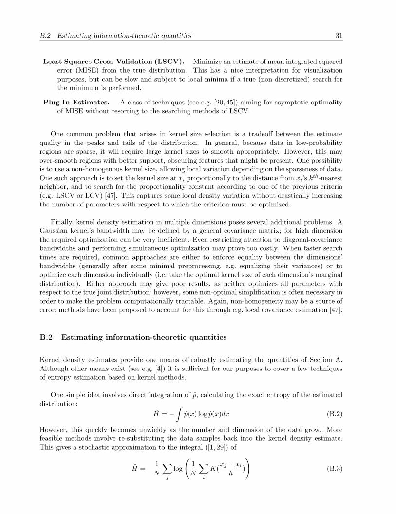
B.2 Estimating information-theoretic quantities 31
Least Squares Cross-Validation (LSCV). Minimize an estimate of mean integrated squarederror (MISE) from the true distribution. This has a nice interpretation for visualizationpurposes, but can be slow and subject to local minima if a true (non-discretized) search forthe minimum is performed.
Plug-In Estimates. A class of techniques (see e.g. [20, 45]) aiming for asymptotic optimalityof MISE without resorting to the searching methods of LSCV.
One common problem that arises in kernel size selection is a tradeoff between the estimatequality in the peaks and tails of the distribution. In general, because data in low-probabilityregions are sparse, it will require large kernel sizes to smooth appropriately. However, this mayover-smooth regions with better support, obscuring features that might be present. One possibilityis to use a non-homogenous kernel size, allowing local variation depending on the sparseness of data.One such approach is to set the kernel size at xi proportionally to the distance from xi’s k
th-nearestneighbor, and to search for the proportionality constant according to one of the previous criteria(e.g. LSCV or LCV) [47]. This captures some local density variation without drastically increasingthe number of parameters with respect to which the criterion must be optimized.
Finally, kernel density estimation in multiple dimensions poses several additional problems. AGaussian kernel’s bandwidth may be defined by a general covariance matrix; for high dimensionthe required optimization can be very inefficient. Even restricting attention to diagonal-covariancebandwidths and performing simultaneous optimization may prove too costly. When faster searchtimes are required, common approaches are either to enforce equality between the dimensions’bandwidths (generally after some minimal preprocessing, e.g. equalizing their variances) or tooptimize each dimension individually (i.e. take the optimal kernel size of each dimension’s marginaldistribution). Either approach may give poor results, as neither optimizes all parameters withrespect to the true joint distribution; however, some non-optimal simplification is often necessary inorder to make the problem computationally tractable. Again, non-homogeneity may be a source oferror; methods have been proposed to account for this through e.g. local covariance estimation [47].
B.2 Estimating information-theoretic quantities
Kernel density estimates provide one means of robustly estimating the quantities of Section A.Although other means exist (see e.g. [4]) it is sufficient for our purposes to cover a few techniquesof entropy estimation based on kernel methods.
One simple idea involves direct integration of p, calculating the exact entropy of the estimateddistribution:
H = −∫
p(x) log p(x)dx (B.2)
However, this quickly becomes unwieldy as the number and dimension of the data grow. Morefeasible methods involve re-substituting the data samples back into the kernel density estimate.This gives a stochastic approximation to the integral ([1, 29]) of
H = − 1
N
∑
j
log
(
1
N
∑
i
K(xj − xi
h)
)
(B.3)

32 C NONPARAMETRIC BELIEF PROPAGATION
or, removing the evaluation datum from the density estimate gives a leave-one-out estimate ([4])with reduced bias
H = − 1
N
∑
j
log
1
N − 1
∑
i6=j
K(xj − xi
h)
(B.4)
Mutual information can then be estimated via Equation (A.2):
I(x; y) = H(x) + H(y)− H(x, y) (B.5)
and KL-divergence as:
D(p||q) = H(x)− 1
N
∑
j
q(xj) (B.6)
Another estimate of entropy, appropriate for variables with a bounded range, is an integrated-square-error (ISE) approximation. This proves to be useful in learning. Suppose that the continuousvariable x takes values in the fixed range [0, 1]. Then, using the definition of entropy and the Taylorexpansion about unity,
H = −∫
p(x) log p(x) dx log x =∞∑
i=1
(x− 1)i
i(B.7)
we can approximate p(x) log p(x) to second order, giving
H ≈ −∫
(p(x)− 1) +(p(x)− 1)2
2dx (B.8)
HISE = −1
2
∫
(1− p(x))2 dx (B.9)
Thus, the negative of the integrated squared distance from the uniform distribution serves asan approximate estimate of entropy, particularly when p is near uniform, the maximum entropydistribution on a bounded interval. One also finds this estimate as another formulation of entropy,the Renyi entropy [10, 15].
For kernel density estimates, the gradient of the integral in Equation (B.9) can be computedexactly in O(N2) operations, a similar efficiency to the stochastic integration estimates of Equa-tions (B.3) and (B.4).
C Nonparametric Belief Propagation
The following text is from [49], appearing in Proceedings, CVPR 2003
C.1 Introduction
Graphical models provide a powerful, general framework for developing statistical models of com-puter vision problems [16, 18, 26]. However, graphical formulations are only useful when combined

C.1 Introduction 33
Markov Chain
Graphical Models
Figure 14: Particle filters assume variables are related by a simple Markov chain. The NBP algorithmextends particle filtering techniques to arbitrarily structured graphical models.
with efficient algorithms for inference and learning. Computer vision problems are particularlychallenging because they often involve high–dimensional, continuous variables and complex, multi-modal distributions. For example, the articulated models used in many tracking applications havedozens of degrees of freedom to be estimated at each time step [46]. Realistic graphical modelsfor these problems must represent outliers, bimodalities, and other non–Gaussian statistical fea-tures. The corresponding optimal inference procedures for these models typically involve integralequations for which no closed form solution exists. Thus, it is necessary to develop families ofapproximate representations, and corresponding methods for updating those approximations.
The simplest method for approximating intractable continuous–valued graphical models is dis-cretization. Although exact inference in general discrete graphs is NP hard [8], approximate infer-ence algorithms such as loopy belief propagation (BP) [41, 51, 54, 56] have been shown to produceexcellent empirical results in many cases. Certain vision problems, including stereo vision [50]and phase unwrapping [17], are well suited to discrete formulations. For problems involving high–dimensional variables, however, exhaustive discretization of the state space is intractable. In somecases, domain–specific heuristics may be used to dynamically exclude those configurations whichappear unlikely based upon the local evidence [9, 16]. In more challenging vision applications, how-ever, the local evidence at some nodes may be inaccurate or misleading, and these approaches willheavily distort the computed estimates.
For temporal inference problems, particle filters [13, 26] have proven to be an effective, and in-fluential, alternative to discretization. They provide the basis for several of the most effective visualtracking algorithms [39, 46]. Particle filters approximate conditional densities nonparametrically asa collection of representative elements. Although it is possible to update these approximationsdeterministically using local linearizations [2], most implementations use Monte Carlo methodsto stochastically update a set of weighted point samples. The stability and robustness of parti-cle filters can often be improved by regularization methods [13, Chapter 12] in which smoothingkernels [40, 47] explicitly represent the uncertainty associated with each point sample.
Although particle filters have proven to be extremely effective for visual tracking problems, theyare specialized to temporal problems whose corresponding graphs are simple Markov chains (seeFigure 14). Many vision problems, however, are characterized by non–causal (e.g., spatial or model–induced) structure which is better represented by a more complex graph. Because particle filters

34 C NONPARAMETRIC BELIEF PROPAGATION
cannot be applied to arbitrary graphs, graphical models containing high–dimensional variables maypose severe problems for existing inference techniques. Even for tracking problems, there is oftenstructure within each time instant (for example, associated with an articulated model) which isignored by standard particle filters.
Some authors have used junction tree representations [34] to develop structured approximateinference techniques for general graphs. These algorithms begin by clustering nodes into cliqueschosen to break the original graph’s cycles. A wide variety of algorithms can then be specifiedby combining an approximate clique variable representation with local methods for updating theseapproximations [11, 32]. For example, Koller et al. [32] propose a framework in which the currentclique potential estimate is used to guide message computations, allowing approximations to begradually refined over successive iterations. However, the sample algorithm they provide is limitedto networks containing mixtures of discrete and Gaussian variables. In addition, for many graphs(e.g. nearest–neighbor grids) the size of the junction tree’s largest cliques grows exponentially withproblem size, requiring the estimation of extremely high–dimensional distributions.
The nonparametric belief propagation (NBP) algorithm we develop in this paper differs fromprevious nonparametric approaches in two key ways. First, for graphs with cycles we do notform a junction tree, but instead iterate our local message updates until convergence as in loopyBP. This has the advantage of greatly reducing the dimensionality of the spaces over which wemust infer distributions. Second, we provide a message update algorithm specifically adaptedto graphs containing continuous, non–Gaussian potentials. The primary difficulty in extendingparticle filters to general graphs is in determining efficient methods for combining the informationprovided by several neighboring nodes. Representationally, we address this problem by associatinga regularizing kernel with each particle, a step which is necessary to make message products welldefined. Computationally, we show that message products may be computed using an efficient localGibbs sampling procedure. The NBP algorithm may be applied to arbitrarily structured graphscontaining a broad range of potential functions, effectively extending particle filtering methods toa much broader range of vision problems.
Following our presentation of the NBP algorithm, we validate its performance on a small Gaus-sian network. We then show how NBP may be combined with parts–based local appearance mod-els [12, 37, 52] to locate and reconstruct occluded facial features.
C.2 Undirected Graphical Models
An undirected graph G is defined by a set of nodes V, and a corresponding set of edges E . Theneighborhood of a node s ∈ V is defined as Γ(s) , {t|(s, t) ∈ E}, the set of all nodes which aredirectly connected to s. Graphical models associate each node s ∈ V with an unobserved, or hidden,random variable xs, as well as a noisy local observation ys. Let x = {xs}s∈V and y = {ys}s∈V denotethe sets of all hidden and observed variables, respectively. To simplify the presentation, we considermodels with pairwise potential functions, for which p (x, y) factorizes as
p (x, y) =1
Z
∏
(s,t)∈E
ψs,t (xs, xt)∏
s∈V
ψs (xs, ys) (C.1)

C.2 Undirected Graphical Models 35
However, the nonparametric updates we present may be directly extended to models with higher–order potential functions.
In this paper, we focus on the calculation of the conditional marginal distributions p (xs | y) forall nodes s ∈ V. These densities provide not only estimates of xs, but also corresponding measuresof uncertainty.
C.2.1 Belief Propagation
For graphs which are acyclic or tree–structured, the desired conditional distributions p (xs | y) canbe directly calculated by a local message–passing algorithm known as belief propagation (BP) [41,56]. At iteration n of the BP algorithm, each node t ∈ V calculates a message mn
ts (xs) to be sentto each neighboring node s ∈ Γ(t):
mnts (xs) = α
∫
xt
ψs,t (xs, xt)ψt (xt, yt)×∏
u∈Γ(t)\s
mn−1ut (xt) dxt (C.2)
Here, α denotes an arbitrary proportionality constant. At any iteration, each node can producean approximation pn(xs | y) to the marginal distributions p (xs | y) by combining the incomingmessages with the local observation potential:
pn(xs | y) = αψs (xs, ys)∏
t∈Γ(s)
mnts (xs) (C.3)
For tree–structured graphs, the approximate marginals, or beliefs, pn(xs | y) will converge to thetrue marginals p (xs | y) once the messages from each node have propagated to every other node inthe graph.
Because each iteration of the BP algorithm involves only local message updates, it can beapplied even to graphs with cycles. For such graphs, the statistical dependencies between BPmessages are not properly accounted for, and the sequence of beliefs pn(xs | y) will not converge tothe true marginal distributions. In many applications, however, the resulting loopy BP algorithmexhibits excellent empirical performance [16, 17]. Recently, several theoretical studies have providedinsight into the approximations made by loopy BP, partially justifying its application to graphswith cycles [51, 54, 56].
C.2.2 Nonparametric Representations
Exact evaluation of the BP update equation (C.2) involves an integration which, as discussed in theIntroduction, is not analytically tractable for most continuous hidden variables. An interesting al-ternative is to represent the resulting message mts (xs) nonparametrically as a kernel–based densityestimate [40, 47]. Let N (x;µ,Λ) denote the value of a Gaussian density of mean µ and covarianceΛ at the point x. We may then approximate mts (xs) by a mixture of M Gaussian kernels as
mts (xs) =M∑
i=1
w(i)s N
(
xs;µ(i)s ,Λs
)
(C.4)

36 C NONPARAMETRIC BELIEF PROPAGATION
where w(i)s is the weight associated with the ith kernel mean µ
(i)s , and Λs is a bandwidth or smoothing
parameter. Other choices of kernel functions are possible [47], but in this paper we restrict ourattention to mixtures of diagonal–covariance Gaussians.
In the following section, we describe stochastic methods for determining the kernel centers µ(i)s
and associated weights w(i)s . The resulting nonparametric representations are only meaningful when
the messages mts (xs) are finitely integrable.1 To guarantee this, it is sufficient to assume that allpotentials satisfy the following constraints:
∫
xs
ψs,t (xs, xt = x) dxs <∞∫
xs
ψs (xs, ys = y) dxs <∞ (C.5)
Under these assumptions, a simple induction argument will show that all messages are normalizable.Heuristically, equation (C.5) requires all potentials to be “informative,” so that fixing the value ofone variable constrains the likely locations of the other. In most application domains, this can betrivially achieved by assuming that all hidden variables take values in a large, but bounded, range.
C.3 Nonparametric Message Updates
Conceptually, the BP update equation (C.2) naturally decomposes into two stages. First, themessage product ψt (xt, yt)
∏
umn−1ut (xt) combines information from neighboring nodes with the
local evidence yt, producing a function summarizing all available knowledge about the hidden vari-able xt. We will refer to this summary as a likelihood function, even though this interpretationis only strictly correct for an appropriately factorized tree–structured graph. Second, this like-lihood function is combined with the compatibility potential ψs,t (xs, xt), and then integrated toproduce likelihoods for xs. The nonparametric belief propagation (NBP) algorithm stochasticallyapproximates these two stages, producing consistent nonparametric representations of the mes-sages mts (xs). Approximate marginals p(xs | y) may then be determined from these messages byapplying the following section’s stochastic product algorithm to equation (C.3).
C.3.1 Message Products
For the moment, assume that the local observation potentials ψt (xt, yt) are represented by weightedGaussian mixtures (such potentials arise naturally from learning–based approaches to model iden-tification [16]). The product of d Gaussian densities is itself Gaussian, with mean and covariancegiven by
d∏
j=1
N (x;µj ,Λj) ∝ N(
x; µ, Λ)
Λ−1 =d∑
j=1
Λ−1j Λ−1µ =
d∑
j=1
Λ−1j µj (C.6)
Thus, a BP update operation which multiplies dGaussian mixtures, each containingM components,will produce another Gaussian mixture withM d components. The weight w associated with product
1Probabilistically, BP messages are likelihood functions mts (xs) ∝ p (y = y | xs), not densities, and are not nec-essarily integrable (e.g., when xs and y are independent).

C.3 Nonparametric Message Updates 37
Msg 1
Msg 2 - -
Msg 3
l1 =?, l2 = 1, l3 = 4 l1 = 4, l2 =?, l3 = 4 l1 = 4, l2 = 3, l3 =?
?.
.
.
��
I
l1 = 3, l2 = 2, l3 = 4
Figure 15: Top row: Gibbs sampler for a product of 3 Gaussian mixtures, with 4 kernels each. New indicesare sampled according to weights (arrows) determined by the two fixed components (solid). The Gibbssampler cycles through the different messages, drawing a new mixture label for one message conditionedon the currently labeled Gaussians in the other messages. Bottom row: After κ iterations through all themessages, the final labeled Gaussians for each message (right, solid) are multiplied together to identify one(left, solid) of the 43 components (left, thin) of the product density (left, dashed).
mixture component N(
x; µ, Λ)
is given by
w ∝
∏dj=1wjN (x;µj ,Λj)
N(
x; µ, Λ) (C.7)
where {wj}dj=1 are the weights associated with the input Gaussians. Note that equation (C.7)produces the same value for any choice of x. Also, in various special cases, such as when all inputGaussians have the same variance Λj = Λ, computationally convenient simplifications are possible.
Since integration of Gaussian mixtures is straightforward, in principle the BP message updatescould be performed exactly by repeated use of equations (C.6,C.7). In practice, however, theexponential growth of the number of mixture components forces approximations to be made. Givend input mixtures of M Gaussian, the NBP algorithm approximates their M d–component productmixture by drawing M independent samples.
Direct sampling from this product, achieved by explicitly calculating each of the product compo-nent weights (C.7), would require O(M d) operations. The complexity associated with this samplingis combinatorial: each product component is defined by d labels {lj}dj=1, where lj identifies a kernel
in the jth input mixture. Although the joint distribution of the d labels is complex, the conditionaldistribution of any individual label lj is simple. In particular, assuming fixed values for {lk}k 6=j ,equation (C.7) can be used to sample from the conditional distribution of lj in O(M) operations.
Since the mixture label conditional distributions are tractable, we may use a Gibbs sampler [18]

38 C NONPARAMETRIC BELIEF PROPAGATION
Given d mixtures of M Gaussians, where {µ(i)j ,Λ
(i)j , w
(i)j }Mi=1 denote the parameters of the jth mixture:
1. For each j ∈ [1 : d], choose a starting label lj ∈ [1 : M ] by sampling p (lj = i) ∝ w(i)j .
2. For each j ∈ [1 : d],
(a) Calculate the mean µ∗ and variance Λ∗ of the product∏
k 6=j N(
x;µ(lk)k ,Λ
(lk)k
)
using equa-
tion (C.6).
(b) For each i ∈ [1 : M ], calculate the mean µ(i) and variance Λ(i) of N (x;µ∗,Λ∗) · N(
x;µ(i)j ,Λ
(i)j
)
.
Using any convenient x, compute the weight
w(i) = w(i)j
N(
x;µ(i)j ,Λ
(i)j
)
N (x;µ∗,Λ∗)
N(
x; µ(i), Λ(i))
(c) Sample a new label lj according to p (lj = i) ∝ w(i).
3. Repeat step 2 for κ iterations.
4. Compute the mean µ and variance Λ of the product∏d
j=1N(
x;µ(lj)j ,Λ
(lj)j
)
. Draw a sample x ∼N(
x; µ, Λ)
.
Algorithm 1: Gibbs sampler for products of Gaussian mixtures.
to draw asymptotically unbiased samples from the product distribution. Details are provided inAlgorithm 1, and illustrated in Figure 15. At each iteration, the labels {lk}k 6=j for d − 1 of theinput mixtures are fixed, and a new value for the jth label is chosen according to equation (C.7). Atthe following iteration, the newly chosen lj is fixed, and another label is updated. This procedurecontinues for a fixed number of iterations κ; more iterations lead to more accurate samples, butrequire greater computational cost. Following the final iteration, the mean and covariance of theselected product mixture component is found using equation (C.6), and a sample point is drawn.To draw M (approximate) samples from the product distribution, the Gibbs sampler requires atotal of O(dκM2) operations.
Although formal verification of the Gibbs sampler’s convergence is difficult, in our experimentswe have observed good performance using far fewer computations than required by direct sampling.Note that the NBP algorithm uses the Gibbs sampling technique differently from classic simulatedannealing procedures [18]. In simulated annealing, the Gibbs sampler updates a single Markovchain whose state dimension is proportional to the graph dimension. In contrast, NBP uses manylocal Gibbs samplers, each involving only a few nodes. Thus, although NBP must run more inde-pendent Gibbs samplers, for large graphs the dimensionality of the corresponding Markov chainsis dramatically smaller.
In some applications, the observation potentials ψt (xt, yt) are most naturally specified by ana-lytic functions. The previously proposed Gibbs sampler may be easily adapted to this case usingimportance sampling [13], as shown in Algorithm 2. At each iteration, the weights used to samplea new kernel label are rescaled by ψt
(
µ(i), yt
)
, the observation likelihood at each kernel’s center.Then, the final sample is assigned an importance weight to account for variations of the analyticpotential over the kernel’s support. This procedure will be most effective when ψt (xt, yt) variesslowly relative to the typical kernel bandwidth.

C.3 Nonparametric Message Updates 39
Given d mixtures of M Gaussians and an analytic function f(x), follow Algorithm 1 with the followingmodifications:
2. After part (b), rescale each computed weight by the analytic value at the kernel center: w(i) ←f(µ(i))w(i).
5. Assign importance weight w = f(x)/f(µ) to the sampled particle x.
Algorithm 2: Gibbs sampler for the product of several Gaussian mixtures with an analytic function f(x).
Given input messages mut (xt) = {µ(i)ut ,Λ
(i)ut , w
(i)ut }Mi=1 for each u ∈ Γ(t) \ s, construct an output message
mts (xs) as follows:
1. Determine the marginal influence ζ(xt) using equation (C.8):
(a) If ψs,t (xs, xt) is a Gaussian mixture, ζ(xt) is the marginal over xt.
(b) For analytic ψs,t (xs, xt), determine ζ(xt) by symbolic or numeric integration.
2. Draw M independent samples {x(i)t }Mi=1 from the product ζ(xt)ψt (xt, yt)
∏
umut (xt) using the Gibbssampler of Algorithms 1-2.
3. For each {x(i)t }Mi=1, sample x
(i)s ∼ ψs,t(xs, xt = x
(i)t ):
(a) If ψs,t (xs, xt) is a Gaussian mixture, x(i)s is sampled from the conditional of xs given x
(i)t .
(b) For analytic ψs,t (xs, xt), importance sampling or MCMC methods may be used as appropriate.
4. Construct mts (xs) = {µ(i)ts ,Λ
(i)ts , w
(i)ts }Mi=1:
(a) Set µ(i)ts = x
(i)s , and w
(i)ts equal to the importance weights (if any) generated in step 3.
(b) Choose {Λ(i)ts }Mi=1 using any appropriate kernel size selection method (see [47]).
Algorithm 3: NBP algorithm for updating the nonparametric message mts (xs) sent from node t to nodes as in equation (C.2).
C.3.2 Message Propagation
In the second stage of the NBP algorithm, the information contained in the incoming messageproduct is propagated by stochastically approximating the belief update integral (C.2). To performthis stochastic integration, the pairwise potential ψs,t (xs, xt) must be decomposed to separate itsmarginal influence on xt from the conditional relationship it defines between xs and xt.
The marginal influence function ζ(xt) is determined by the relative weight assigned to all xs
values for each xt:
ζ(xt) =
∫
xs
ψs,t (xs, xt) dxs (C.8)
The NBP algorithm accounts for the marginal influence of ψs,t (xs, xt) by incorporating ζ(xt) intothe Gibbs sampler. If ψs,t (xs, xt) is a Gaussian mixture, extraction of ζ(xt) is trivial. Alternately,if ζ(xt) can be evaluated (or approximated) pointwise, analytic pairwise potentials may be dealtwith using importance sampling. In the common case where pairwise potentials depend only onthe difference between their arguments (ψs,t (x, x) = ψs,t (x − x)), ζ(xt) is constant and can beneglected.

40 C NONPARAMETRIC BELIEF PROPAGATION
To complete the stochastic integration, each particle x(i)t produced by the Gibbs sampler is
propagated to node s by sampling x(i)s ∼ ψs,t(xs, x
(i)t ). Note that the assumptions of Section C.2.2
ensure that ψs,t(xs, x(i)t ) is normalizable for any x
(i)t . The method by which this sampling step is
performed will depend on the specific functional form of ψs,t (xs, xt), and may involve importancesampling or MCMC techniques. Finally, having produced a set of independent samples from thedesired output message mts (xs), NBP must choose a kernel bandwidth to complete the nonpara-metric density estimate. There are many ways to make this choice; for the results in this paper,we used the computationally efficient “rule of thumb” heuristic [47].
The NBP message update procedure developed in this section is summarized in Algorithm 3.Note that various stages of this algorithm may be simplified in certain special cases. For example,if the pairwise potentials ψs,t (xs, xt) are mixtures of only one or two Gaussians, it is possibleto replace the sampling and kernel size selection of steps 3–4 by a simple deterministic kernelplacement. However, these more sophisticated updates are necessary for graphical models withmore expressive priors, such as those used in Section C.5.
C.4 Gaussian Graphical Models
Gaussian graphical models provide one of the few continuous distributions for which the BP algo-rithm may be implemented exactly [54]. For this reason, Gaussian models may be used to test theaccuracy of the nonparametric approximations made by NBP. Note that we cannot hope for NBPto outperform algorithms (like Gaussian BP) designed to take advantage of the linear structureunderlying Gaussian problems. Instead, our goal is to verify NBP’s performance in a situationwhere exact comparisons are possible.
We have tested the NBP algorithm on Gaussian models with a range of graphical structures,including chains, trees, and grids. Similar results were observed in all cases, so here we only presentdata for a single typical 5 × 5 nearest–neighbor grid (as in Figure 14), with randomly selectedinhomogeneous potential functions. To create the test model, we drew independent samples fromthe single correlated Gaussian defining each of the graph’s clique potentials, and then formed anonparametric density estimate based on these samples. Although the NBP algorithm could havedirectly used the original correlated potentials, sample–based models are a closer match for theinformation available in many vision applications (see Section C.5).
For each node s ∈ V, Gaussian BP converges to a steady–state estimate of the marginal meanµs and variance σ2
s after about 15 iterations. To evaluate NBP, we performed 15 iterations of theNBP message updates using several different particle set sizes M ∈ [10, 400]. We then found themarginal mean µs and variance σ2
s estimates implied by the final NBP density estimates. For eachtested particle set size, the NBP comparison was repeated 100 times.
Using the data from each NBP trial, we computed the error in the mean and variance estimates,normalized so each node behaved like a unit–variance Gaussian:
µs =µs − µs
σsσ2
s =σ2
s − σ2s√
2σ2s
(C.9)
Figure 16 shows the mean and variance of these error statistics, across all nodes and trials, for
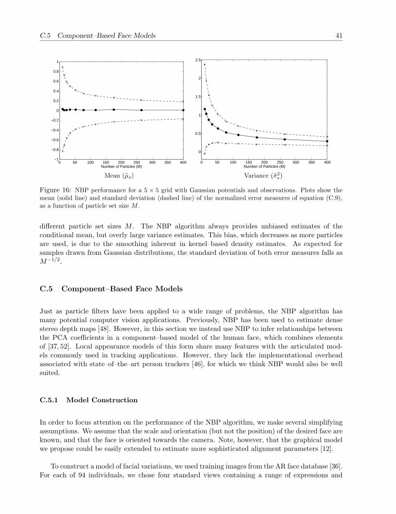
C.5 Component–Based Face Models 41
0 50 100 150 200 250 300 350 400−1
−0.8
−0.6
−0.4
−0.2
0
0.2
0.4
0.6
0.8
1
Number of Particles (M)0 50 100 150 200 250 300 350 400
0
0.5
1
1.5
2
2.5
Number of Particles (M)
Mean (µs) Variance (σ2s)
Figure 16: NBP performance for a 5 × 5 grid with Gaussian potentials and observations. Plots show themean (solid line) and standard deviation (dashed line) of the normalized error measures of equation (C.9),as a function of particle set size M .
different particle set sizes M . The NBP algorithm always provides unbiased estimates of theconditional mean, but overly large variance estimates. This bias, which decreases as more particlesare used, is due to the smoothing inherent in kernel–based density estimates. As expected forsamples drawn from Gaussian distributions, the standard deviation of both error measures falls asM−1/2.
C.5 Component–Based Face Models
Just as particle filters have been applied to a wide range of problems, the NBP algorithm hasmany potential computer vision applications. Previously, NBP has been used to estimate densestereo depth maps [48]. However, in this section we instead use NBP to infer relationships betweenthe PCA coefficients in a component–based model of the human face, which combines elementsof [37, 52]. Local appearance models of this form share many features with the articulated mod-els commonly used in tracking applications. However, they lack the implementational overheadassociated with state–of–the–art person trackers [46], for which we think NBP would also be wellsuited.
C.5.1 Model Construction
In order to focus attention on the performance of the NBP algorithm, we make several simplifyingassumptions. We assume that the scale and orientation (but not the position) of the desired face areknown, and that the face is oriented towards the camera. Note, however, that the graphical modelwe propose could be easily extended to estimate more sophisticated alignment parameters [12].
To construct a model of facial variations, we used training images from the AR face database [36].For each of 94 individuals, we chose four standard views containing a range of expressions and

42 C NONPARAMETRIC BELIEF PROPAGATION
Figure 17: Two of the 94 training subjects fromthe AR face database. Each subject was pho-tographed in these four poses.
(a) (b) (c)
Figure 18: PCA–based facial component model.(a) Control points and feature masks for each ofthe five components. Note that the two mouthmasks overlap. (b) Mean features. (c) Graphicalprior relating the position and PCA coefficientsof each component.
Figure 19: Empirical joint densities of six different pairs of PCA coefficients, selected from the three mostsignificant PCA bases at each node. Each plot shows the corresponding marginal distributions along thebottom and right edges. Note the multimodal, non–Gaussian relationships.
lighting conditions (see Figure 17). We then manually selected five feature points (eyes, nose andmouth corners) on each person, and used these points to transform the images to a canonicalalignment. These same control points were used to center the feature masks shown in Figure 18(a).In order to model facial variations, we computed a principal component analysis (PCA) of each ofthe five facial components [37]. The resulting component means are shown in Figure 18(b). Foreach facial feature, only the 10 most significant principal components were used in the subsequentanalysis.
After constructing the PCA bases, we computed the corresponding PCA coefficients for eachindividual in the training set. Then, for each of the component pairs connected by edges in Fig-ure 18(c), we determined a kernel–based nonparametric density estimate of their joint coefficientprobabilities. Figure 19 shows several marginalizations of these 20–dimensional densities, eachof which relates a single pair of coefficients (e.g., the first nose and second left eye coefficients).Note that all of these plots involve one of the three most significant PCA bases for each compo-

C.5 Component–Based Face Models 43
nent, so they represent important variations in the data. We can clearly see that simple Gaussianapproximations would lose most of this data set’s interesting structure.
Using these nonparametric estimates of PCA coefficient relationships and the graph of Fig-ure 18(c), we constructed a joint prior model for the location and appearance of each facial compo-nent. The hidden variable at each node is 12 dimensional (10 PCA coefficients plus location). Weapproximate the true clique potentials relating neighboring PCA coefficients by the correspondingjoint probability estimates [16]. We also assume that differences between feature positions areGaussian distributed, with a mean and variance estimated from the training set.
C.5.2 Estimation of Occluded Features
In this section, we apply the graphical model developed in the previous section to the simultaneouslocation and reconstruction of partially occluded faces. Given an input image, we first localizethe region most likely to contain a face using a standard eigenface detector [37] trained on partialface images. This step helps to prevent spurious detection of background detail by the individualcomponents. We then construct observation potentials by scanning each feature mask across theidentified subregion, producing the best 10–component PCA representation y of each pixel win-dow y. For each tested position, we create a Gaussian mixture component with mean equal tothe matching coefficients, and weight proportional to exp
{
−||y − y||2/2σ2}
. To account for out-liers produced by occluded features, we add a single zero mean, high–variance Gaussian to eachobservation potential, weighted to account for 20% of the total likelihood.
We tested the NBP algorithm on uncalibrated images of individuals not found in the trainingset. Each message was represented by M = 100 particles, and each Gibbs sampling operation usedκ = 100 iterations. Total computation time for each image was a few minutes on a Pentium 4workstation. Due to the high dimensionality of the variables in this model, and the presence of theocclusion process, discretization is completely intractable. Therefore, we instead compare NBP’sestimates to the closed form solution obtained by fitting a single Gaussian to each of the empiricallyderived mixture densities.
Figure 20 shows inference results for two images of a man concealing his mouth. In one imagehe is smiling, while in the other he is not. Using the relationships between eye and mouth shapelearned from the training set, NBP is able to correctly infer the shape of the concealed mouth. Incontrast, the Gaussian approximation loses the structure shown in Figure 19, and produces twomouths which are visually equal to the mean mouth shape. While similar results could be obtainedusing a variety of ad hoc classification techniques, it is important to note that the NBP algorithmwas only provided unlabeled training examples.
Figure 21 shows inference results for two images of a woman concealing one eye. In one image,she is seen under normal illumination, while in the second she is illuminated from the left by abright light. In both cases, the concealed eye is correctly estimated to be structurally similar tothe visible eye. In addition, NBP correctly modifies the illumination of the occluded eye to matchthe intensity of the corresponding mouth corner. This example shows NBP’s ability to seamlesslyintegrate information from multiple nodes to produce globally consistent estimates.

44 D HYPOTHESIS TESTING OVER FACTORIZATIONS FOR DATA ASSOCIATION
C.6 Discussion
We have developed a nonparametric sampling–based variant of the belief propagation algorithmfor graphical models with continuous, non–Gaussian random variables. Our parts–based facialmodeling results demonstrate NBP’s ability to infer sophisticated relationships from training data,and suggest that it may prove useful in more complex visual tracking problems. We hope that NBPwill allow the successes of particle filters to be translated to many new computer vision applications.
Acknowledgments
The authors would like to thank Ali Rahimi for his help with the facial appearance modelingapplication.
D Hypothesis Testing over Factorizations for Data Association
The following text is from [24], appearing in Proceedings, Information Processing in Sensor Net-works 2003.
D.1 Introduction
Data association describes the problem of partitioning observations into like sets. This is a commonproblem in networks of sensors – multiple signals are received by several sensors, and one mustdetermine which signals at different sensors correspond to the same source.
In many collaborative sensing scenarios, the signal models are assumed to be known and fullyspecified a priori. With such models, it is possible to formulate and use optimal hypothesis testsfor data association. However, real-world uncertainty often precludes strong modelling assump-tions. For example, it is difficult to analytically quantify dependence between data of differentmodalities. Additionally, nonlinear effects and inhomogenous media create complex interactionsand uncertainty. When applicable, a learning/estimation based approach is appealing, but in theonline case requires that one learn the signal distributions while simultaneously performing thetest. For example, this is possible for data association because it is a test described in terms of thedistribution form, in particular as a test over factorization and independence.
We show that the optimal likelihood test between two factorizations of a density learned fromthe data can be expressed in terms of mutual information. Furthermore, the analysis resultsin a clear decomposition of terms related to statistical dependence (i.e. factorization) and thoserelated to modelling assumptions. We propose the use of kernel density methods to estimatethe distributions and mutual information from data. In the case of high-dimensional data, wherelearning a distribution is impractical, this can be done efficiently by finding statistics which captureits interaction. Furthermore, the criterion for learning these statistics is also expressed in terms

D.1 Introduction 45
Gaussian Neutral NBP Gaussian Smiling NBP
Figure 20: Simultaneous estimation of location (top row) and appearance (bottom row) of an occludedmouth. Results for the Gaussian approximation are on the left of each panel, and for NBP on the right. Byobserving the squinting eyes of the subject (right), and exploiting the feature interrelationships represented inthe trained graphical model, the NBP algorithm correctly infers that the occluded mouth should be smiling.A parametric Gaussian model doesn’t capture these relationships, producing estimates indistinguishablefrom the mean face.
Gaussian Ambient Lighting NBP Gaussian Lighted from Left NBP
Figure 21: Simultaneous estimation of location (top row) and appearance (bottom row) of an occluded eye.NBP combines information from the visible eye and mouth to determine both shape and illumination of theoccluded eye, correctly inferring that the left eye should brighten under the lighting conditions shown atright. The Gaussian approximation fails to capture these detailed relationships.

46 D HYPOTHESIS TESTING OVER FACTORIZATIONS FOR DATA ASSOCIATION
of mutual information. The estimated mutual information of these statistics can be used as anapproximation to the optimal likelihood ratio test, by training the statistics to minimize a boundon the approximation error.
We will begin by describing a data association example between a pair of sensors, each observingtwo targets. We show first how the optimal hypothesis test changes in the absence of a knownsignal model and express the resulting test in terms of information. We then discuss how one mayuse summarizing features to estimate the mutual information efficiently and robustly using kernelmethods. This can yield a tractable estimate of the hypothesis test when direct estimation of theobservations’ distribution is infeasible. Finally, we present an algorithmic extension of these ideasto the multiple target case.
D.2 An Information-Theoretic Interpretation of Data Association
Data association can be cast as a hypothesis test between density factorizations over measurements.As we will show, there is a natural information-theoretic interpretation of this hypothesis test, whichdecomposes the test into terms related to statistical dependency and terms related to modellingassumptions. Consequently, one can quantify the contribution of prior knowledge as it relates to aknown model; but more importantly, in the absence of a prior model one can still achieve a degreeof separability between hypotheses by estimating statistical dependency only. Furthermore, as weshow, one can do so in a low-dimensional feature space so long as one is careful about preservinginformation related to the underlying hypothesis.
Consider the following example problem, which illustrates an application of data associationwithin tracking problems. Suppose we have a pair of widely spaced acoustic sensors, where eachsensor is a small array of many elements. Each sensor produces an observation of the source andan estimate of bearing, which in itself is insufficient to localize the source. However, triangulationof bearing measurements from multiple sensors can be used to estimate the target location. For asingle target, a pair of sensors is sufficient to perform this triangulation.
However, complications arise when there are multiple targets within a pair of sensors’ fieldsof view. Each sensor determines two bearings; but this yields four possible locations for only twotargets, as depicted in Figure 22. With only bearing information, there is no way to know which oneof these target pairs is real, and which is the artifact. We will show that it is possible to address thisambiguity under the assumption that the sources are statistically independent, without requiringa prior model of the relationship between observations across sensors.
D.2.1 Mutual Information
Mutual information is a quantity characterizing the statistical dependence between two randomvariables. Although most widely known for its application to communications (see e.g. [10]), hereit arises in the context of discrimination and hypothesis testing [33].
Correlation is equivalent to mutual information only for jointly Gaussian random variables. The

D.2 An Information-Theoretic Interpretation of Data Association 47
�!�"�#�$%�& �!�"�#�$ %�'
&�(
'�(&�)
'�)
Figure 22: The data association problem: two pairs of measurements results in estimated targets at either thecircles or the squares; but which remains ambiguous.
0 0.2 0.4 0.6 0.8 1 1.2 1.4 1.60
0.05
0.1
0.15
0.2
0.25
0.3
0.35
0.4
0.45
(a) θ = 0 (b) θ = π6 (c) θ = π
4 (d) I(θ)
Figure 23: Two variables x, y with joint distributions (a-c) are uncorrelated but not necessarily independent – (d)shows mutual information as a function of the angle of rotation θ.
common assumption of Gaussian distributions and its computational efficiency have given it wideapplicability to association problems. However, there are many forms of dependency which are notcaptured by correlation.
For example, Figure 23(a-c) shows three non-Gaussian joint distributions characterized by asingle parameter θ, indicating an angle of rotation with respect to the random variables x, y.Although the correlation between x and y is zero for all θ, the plot of mutual information as afunction of θ (Figure 23(d)) demonstrates that for many θ, x and y are far from independent. Thisillustrates how mutual information as a measure of dependence differs from correlation.
D.2.2 Data Association as a Hypothesis Test
Let us assume that we receive N i.i.d. observations of each source at each of the two sensors.When a full distribution is specified for the observed signals, we have a hypothesis test over known,factorized models
H1 : [A1, B1, A2, B2]k ∼ pH1(A1, B1)pH1
(A2, B2)
H2 : [A1, B1, A2, B2]k ∼ pH2(A1, B2)pH2
(A2, B1)
for k ∈ [1 : N ]
(D.1)
with corresponding (normalized) log-likelihood ratio
1
NlogL =
1
N
N∑
k=1
[
logpH1
([A1, B1]k)pH1([A2, B2]k)
pH2([A1, B2]k)pH2
([A2, B1]k)
]
(D.2)

48 D HYPOTHESIS TESTING OVER FACTORIZATIONS FOR DATA ASSOCIATION
As N grows large, the (normalized) log-likelihood approaches its expected value, which can beexpressed in terms of mutual information (MI) and Kullback-Leibler (KL) divergence. Under H1
this value is
EH1[logL] =IH1
(A1;B1) + IH1(A2;B2)+
D(pH1(A1), . . . , pH1
(B2)‖pH2(A1, . . . , B2))
(D.3)
and similarly when H2 is true:
EH2[logL] =− IH2
(A1;B2)− IH2(A1;B2)−
D(pH2(A1), . . . , pH2
(B2)‖pH1(A1, . . . , B2))
(D.4)
The expected value of Equation (D.3) can be grouped in two parts – an information part (the twoMI terms) measuring statistical dependency across sensors, and a model mismatch term (the KL-divergence) measuring difference between the two models. We begin by examining the large-samplelimits of the likelihood ratio test, expressed in terms of its expected value; when this likelihoodratio is not available we see that another estimator for the same quantity may be substituted.
Often the true distributions pHiare unknown, e.g. due to uncertainty in the source densities or
the medium of signal propagation. Consider what might be done with estimates of the densitiesbased on the empirical data to be tested. Note that this allows us to learn densities without requiringmultiple trials under similar conditions. We can construct estimates assuming the factorizationunder either hypothesis, but because observations are only available for the true hypothesis ourestimates of the other will necessarily be incorrect. Specifically, let pHi
(·) be a consistent estimateof the joint distribution assuming the factorization under Hi and let pHi
(·) denote its limit; thenwe have
if H1 is true,
pH1→ pH1
= pH1(A1, B1)pH1
(A2, B2)
pH2→ pH2
= pH1(A1)pH1
(B1)pH1(A2)pH1
(B2)
if H2 is true,
pH1→ pH1
= pH2(A1)pH2
(B1)pH2(A2)pH2
(B2)
pH2→ pH2
= pH2(A1, B2)pH2
(A2, B1)
(D.5)
Thus when pHiassumes the correct hypothesis we converge to the correct distribution, while as-
suming the incorrect hypothesis leads to a fully factored distribution. This is similar to issuesarising in generalized likelihood ratio (GLR) tests [31].
We proceed assuming that our estimates have negligible error, and analyze the behavior oftheir limit p(·); we will examine the effect of error inherent in finite estimates p(·) later. Now theexpectation of the log-likelihood ratio can be expressed solely in terms of the mutual informationbetween the observations. Under H1 this is
EH1[log L] = EH1
[
logpH1
(A1, B1)pH1(A2, B2)
pH2(A1, B2)pH2
(A2, B1)
]
= I(A1;B1) + I(A2;B2)

D.2 An Information-Theoretic Interpretation of Data Association 49
and similarly under H2,
EH2[log L] = −I(A1;B2)− I(A2;B1)
Notice in particular that the KL-divergence terms stemming from model mismatch in Equation (D.3)have vanished. This is due to the fact that both models are estimated from the same data, andquantifies the increased difficulty of discrimination when the models are unknown. We can writethe expectation independent of which hypothesis is true as
E[log L] = I(A1;B1) + I(A2;B2)− I(A1;B2)− I(A2;B1) (D.6)
since for either hypothesis, the other two terms above will be zero; this casts the average log-likelihood ratio as an estimator of mutual information.
We have not assumed that the true distributions p(·) have any particular form, and thereforemight consider using nonparametric methods to ensure that our estimates converge under a widevariety of true distributions. However, if the observations are high-dimensional such methodsrequire an impractical number of samples in order to obtain accurate estimates. In particular, thismeans that the true likelihood ratio cannot be easily calculated, since it involves estimation andevaluation of high-dimensional densities. However, the log-likelihood ratio is acting as an estimatorof the mutual information, and we may instead substitute another, more tractable estimate ofmutual information if available.
Direct estimation of the MI terms above using kernel methods also involves estimating high-dimensional distributions, but one can express it succinctly using features which summarize thedata interaction. We explore ways of learning such features, and shall see that the quality criterionfor summarization is expressed as the mutual information between features estimated in a low-dimensional space.
Let us suppose initially that we possess low-dimensional sufficient statistics for the data. Al-though finding them may be difficult, we know that for the data association problem sufficientstatistics should exist, since the true variable of interest, correspondence, is summarized by a single
scalar likelihood. More precisely, let fAj
i be a low-dimensional feature of Aj and fAj
i its comple-
ment, such that there is a bijective transformation between Aj and [fAj
i , fAj
i ] (and similarly forBk). If the following relation holds,
pHi(Aj , Bk) = pHi
(fAj
i , fAj
i , fBk
i , fBk
i )
= pHi(f
Aj
i , fBk
i )pHi(f
Aj
i |fAj
i )pHi(fBk
i |fBk
i )(D.7)
then the log-likelihood ratio of Equation (D.6) can be written exactly as
E[log L] = I(fA1
1 ; fB1
1 ) + I(fA2
1 ; fB2
1 )− I(fA1
2 ; fB2
2 )− I(fA2
2 ; fB1
2 ) (D.8)
Although sufficient statistics are likely to exist, it may be difficult or impossible to find them
exactly. If the features fAj
i and fBk
i are not sufficient, several divergence terms must be added to
Equation (D.8). For any set of features satisfying pHi(Aj , Bk) = pHi
(fAj
i , fAj
i , fBk
i , fBk
i ), we canwrite
E[log L] = I1;11 + I2;2
1 − I1;22 − I2;1
2 +D1;11 +D2;2
1 −D1;22 −D2;1
2 (D.9)

50 D HYPOTHESIS TESTING OVER FACTORIZATIONS FOR DATA ASSOCIATION
where for brevity we have used the notation
Ij;ki = I(f
Aj
i ; fBk
i )
Dj,ki = D(p(Aj , Bk)‖p(fAj
i , fBk
i )p(fAj
i |fAj
i )p(fBk
i |fBk
i ))
The data likelihood of Equation (D.9) contains a difference of the divergence terms from eachhypothesis. Notice, however, that only the divergence terms involve high-dimensional data; themutual information is calculated between low-dimensional features. Thus if we discard the di-vergence terms we can avoid all calculations on the high-dimensional compliment features f . Wewould like to minimize the effect on our estimate of the likelihood ratio, but cannot estimate theterms directly without evaluating high-dimensional densities. However, by nonnegativity of theKL-divergence we can bound the difference by the sum of the divergences:
∣
∣
∣D1;11 +D2;2
1 −D1;22 −D2;1
2
∣
∣
∣ ≤ D1;11 +D2;2
1 +D1;22 +D2;1
2 (D.10)
We then minimize this bound by minimizing the individual terms, or equivalently maximizing eachmutual information term (which can be done in the low-dimensional feature space). Note thatthese four optimizations are decoupled from each other.
Finally, it is unlikely that with finite data our estimates p(·) will have converged to the limitp(·). Thus we will also have divergence terms from errors in the density estimates:
E[log L] =I1;11 + I2;2
1 − I1;22 − I2;1
2
+D(pH1‖pH1
)−D(pH2‖pH2
)(D.11)
where the I indicate the mutual information of the density estimates. Once again we see a differencein divergence terms; in this case minimization of the bound means choosing density estimates whichconverge to the true underlying distributions as quickly as possible. Note that if pH1
(·) is not aconsistent estimator for the distribution pHi
(·), the individual divergence terms above will never beexactly zero.
Thus we have an estimate of the true log-likelihood ratio between factorizations of a learneddistribution, computed over a low-dimensional space:
E[log L] =I(fA1
1 ; fB1
1 ) + I(fA2
1 ; fB2
1 )− I(fA1
2 ; fB2
2 )
− I(fA2
2 ; fB1
2 ) + divergence terms(D.12)
where maximizing the I with regard to the features fXj
i minimizes a bound on the ignored diver-gence terms. We can therefore use estimates of the mutual information over learned features as anestimate of the true log-likelihood ratio for hypothesis testing.
D.3 Algorithmic Details
The derivations above give general principles by which one may design an algorithm for dataassociation using low-dimensional sufficient statistics. Two primary elements are necessary:
1. a means of estimating entropy, and by extension mutual information, over samples, and

D.3 Algorithmic Details 51
2. a means of optimizing that estimate over the parameters of the sufficient statistic.
We shall address each of these issues in turn.
D.3.1 Estimating Mutual Information
In estimating mutual information, we wish to avoid strong prior modelling assumptions, i.e. jointlyGaussian measurements. There has been considerable research into useful nonparametric methodsfor estimating information-theoretic quantities; for an overview, see e.g. [4].
Kernel density estimation methods are often used as an appealing alternative when no priorknowledge of the distribution is available. Similarly, these kernel-based methods can be used toestimate mutual information effectively. Using estimates with smooth, differentiable kernel shapeswill also yield simple calculations of a gradient for mutual information, which will prove to beuseful in learning. An issue one must consider is that the quality of the estimate degrades as thedimensionality grows; thus we perform the estimate in a low-dimensional space.
To use kernel methods for density estimation requires two basic choices, a kernel shape anda bandwidth or smoothing parameter. For the former, we use Gaussian kernel functions Kσ(x) =
(2πσ2)−1
2 exp{−x2/2σ2}, where σ controls the bandwidth. This ensures that our estimate is smoothand differentiable everywhere. There are a number of ways to choose kernel bandwidth automati-cally (see e.g. [47]). Because we intend to use these density estimates for likelihood evaluation andmaximization, it is sensible to make this the criterion for bandwidth as well; we therefore make useof a leave-one-out maximum likelihood bandwidth, given by
arg maxσ
− 1
N
∑
j
log
1
N − 1
∑
i6=j
Kσ(xj − xi)
(D.13)
Because our variables of interest are continuous, it is convenient to write the mutual informationin terms of joint and marginal entropy, as:
I(fAj
i ; fBk
i ) = H(fAj
i ) +H(fBk
i )−H(fAj
i , fBk
i ) (D.14)
There are a number of possible kernel-based estimates of entropy available [4]. In practice we useeither a leave-one-out resubstitution estimate:
HRS(x) = − 1
N
∑
j
log
1
N − 1
∑
i6=j
Kσ(xj − xi)
(D.15)
or an integrated squared error estimate from [15]:
HISE =H(1)− 1
2
∫
(1− p(x))2 dx (D.16)

52 D HYPOTHESIS TESTING OVER FACTORIZATIONS FOR DATA ASSOCIATION
where 1 is the uniform density on a fixed range, and
p(x) =1
N
∑
j
Kσ(x− xj)
These methods have different interpretations – the former is a stochastic estimate of the trueentropy, while the latter can be considered an exact calculation of an entropy approximation. Inpractice both of these estimates produce similar results. Both estimates may also be differentiatedwith respect to their arguments, yielding tractable gradient estimates useful in learning.
D.3.2 Learning Sufficient Statistics
In order to learn sufficient or relatively sufficient statistics, we must define a function from ourhigh-dimensional observation space to the low-dimensional space over which we are able to calculatemutual information. By choosing a function which admits a simple gradient-based update of theparameter values, we can use gradient ascent to train our function towards a local informationmaximum [14, 23].
Often, quite simple statistic forms will suffice. For example, all of the examples below wereperformed using a simple linear combination of the input variables, passed through a hyperbolictangent function to threshold the output range:
f(x = [x1 . . . xd]) = tanh(∑
i
wixi) (D.17)
That is, using the method of [14, 23] we apply gradient ascent of mutual information between theassociated features with respect to the weight parameters wi.
However, the methods are applicable to any function which can be trained with gradient es-timates, allowing extension to much more complex functional forms. In particular, multiple layerperceptrons are a generalization of the above form which, allowed sufficient complexity, can act asa universal function approximator [6].
We may also wish to impose a capacity control or complexity penalty on the model (e.g. regu-larization). In practice, we put a penalty on the absolute sum of the linear weights (adding to thegradient a constant bias towards zero) to encourage sparse values.
D.4 Data Association of Two Sources
We illustrate the technique above with two examples on synthetic data. The first is a simulation ofdispersive media – an all-pass filter with nonlinear phase characteristics controlled by an adjustableparameter α. The phase response for three example values of α are given in Figure 24(a). SensorA observes two independent signals of bandpassed i.i.d. Gaussian noise, while sensor B observesthe allpass-filtered versions of A.

D.4 Data Association of Two Sources 53
0 0.1 0.2 0.3 0.4 0.5 0.6 0.7 0.8 0.9 10
5
10
15
20
25
30
35
40
45
50
0 0.5 1 1.50
0.05
0.1
0.15
0.2
0.25
0.3
0.35
0.4
0.45
0.5
0 0.5 1 1.50
0.2
0.4
0.6
0.8
1
1.2
1.4
1.6
1.8
2
(a) (b) (c)
Figure 24: Data association across a nonlinear phase all-pass filter: tunable filter (a) yields correlations (b) andmutual information (c).
If the filter characteristics are known, the optimal correspondence test is given by applying theinverse filter to B followed by finding its correlation with A. However when the filter is not known,estimating the inverse filter becomes a source reconstruction problem. Simple correlation of A andB begins to fail as the phase becomes increasingly nonlinear over the bandwidth of the sources. Theupper curve of Figure 24(b) shows the maximum correlation coefficient between correct pairingsof A and B over all time shifts, averaged over 100 trials. Dotted lines indicate the coefficient’sstandard deviation over the trials. To determine significance, we compare this to a baseline ofthe maximum correlation coefficient between incorrect pairings. The region of overlap indicatesnonlinear phases for which correlation cannot reliably determine correspondence.
Figure 24(c) shows an estimate of mutual information between the Fourier spectra of A andB, constructed in the manner outlined above. As α increases, the mutual information estimateassumes a steady-state value which remains separated from the baseline estimate and can accuratelydetermine association.
The second example relates observations of non-overlapping Fourier spectra. Suppose that weobserve a time series and would like to determine whether some higher-frequency observations areunrelated, or are a result of observing some nonlinear function (and thus harmonics) of the originalmeasurements. We simulate this situation by creating two independent signals, passing themthrough a nonlinearity, and relating high-passed and low-passed observations. Sensor A observesthe signals’ lower half spectrum, and sensor B their upper half.
Synthetic data illustrating this can be seen in Figures 25-26. For Figure 25 we create a narrow-band signal whose center frequency is modulated at one of two different rates, and pass it througha cubic nonlinearity. In the resulting filtered spectra (shown in Figure 25(a-d)), the correct pairingis clear by inspection. Scatterplots of the trained features (see Figure 25(e-h)) show that indeed,features of the correct pairings have high mutual information while incorrect pairings have nearlyindependent features.
Figure 26 shows the same test repeated with wideband data – Gaussian noise is passed througha cubic nonlinearity, and the resulting signal is separated into high- and low-frequency observations,shown in Figure 26(a-d). The resulting structure is less obvious, both visually and to our estimatesof mutual information (Figure 26(e-h)), but the correct pairing is still found.

54 D HYPOTHESIS TESTING OVER FACTORIZATIONS FOR DATA ASSOCIATION
(a) A1 (b) A2 (e) A1 ↔ B1 (f) A1 ↔ B2
(c) B1 (d) B2 (g) A2 ↔ B1 (h) A2 ↔ B2
Figure 25: Associating non-overlapping harmonic spectra: the correct pairing of data sets (a-d) is easy to spot;the learned features yield MI estimates which are high for correct pairings (e,h) and low for incorrect pairings (f,g).
(a) A1 (b) A2 (e) A1 ↔ B1 (f) A1 ↔ B2
(c) B1 (d) B2 (g) A2 ↔ B1 (h) A2 ↔ B2
Figure 26: Associating non-overlapping wideband harmonic spectra: though the correct pairing is harder to seethan Figure 25, the estimated MI is still higher for the correct hypothesis (e,h).
D.5 Extension to Many Sources
For the problem described above, the presence of only two targets means the data associationproblem can be expressed as a test between two hypotheses. However, as the number of targetsis increased, the combinatorial nature of the hypothesis test makes evaluation of each hypothesisinfeasible. Approximate methods which determine a correspondence without this computationalburden offer an alternative which may be particularly attractive in the context of sensor networks.We describe an extension of the above method to perform data association between many targetswithout requiring evaluation of all hypotheses.

D.5 Extension to Many Sources 55
Let us re-examine the problem of Section D.2, but allow both sensors to receive separate ob-servations from M independent targets, denoted A1, . . . , AM and B1, . . . , BM . One may still applyestimates of MI to approximate the hypothesis test as described in Section D.2.2, but direct applica-tion will require that mutual information be estimated for each of the M 2 data pairs – a potentiallycostly operation.
However, we suggest an approximate means of evaluating the same test which does not computeeach MI estimate. We can solve the data association problem by finding features which summarizeall the signals received at a particular sensor. A test can then be performed on the learned featurecoefficients directly, rather than computing all individual pairwise likelihoods.
Let us denote the concatenation of all signals from sensor A by [A1, . . . , AM ]. One can learnfeatures which maximize mutual information between this concatenated vector and a particular
signal Bj ; we denote the feature of Bj by fBj
A , and the feature of [A1, . . . , AM ] by f[A1,...,AM ]j .
Again, let us consider the linear statistics of Section D.3.2:
fBj
A = tanh(∑
i
wiBij) (D.18)
f[A1,...,AM ]j = tanh(
∑
i,k
wi,AkAi
k) (D.19)
where Aik (Bi
j) indicates the ith dimension of the signal Ak (Bj).
We now consider tests based on the absolute deviation of the feature coefficients for each signalAk:
∑
i
|wi,Ak|
Under the assumption of independent sources, mutual information exists only between the correctlyassociated signals; i.e. if As and Bt represent a correct association, we have
I(As;Bt) = I([A1, . . . , AM ];Bt)
= I(As; [B1, . . . , BM ])
We may then analyze the mutual information of a particular feature
I(f[A1,...,AM ]t ; fBt
A ) = I(tanh(∑
i,k
wi,AkAi
k); fBt
A )
= I(∑
i,k
wi,AkAi
k; fBt
A )
=∑
k
I(∑
i
wi,AkAi
k; fBt
A )
= I(∑
i
wi,AsAi
s; fBt
A )
Thus, for k 6= s the weights wi,Akhave no contribution to the mutual information. This tells us that
among all features with maximal MI, the one with minimum absolute deviation∑
i,k |wi,Ak| has
support only on As. Whether distributions exist such that no linear feature captures dependence(i.e. I(fA
t ; fBt
A ) = 0 for all linear f) is an open question.
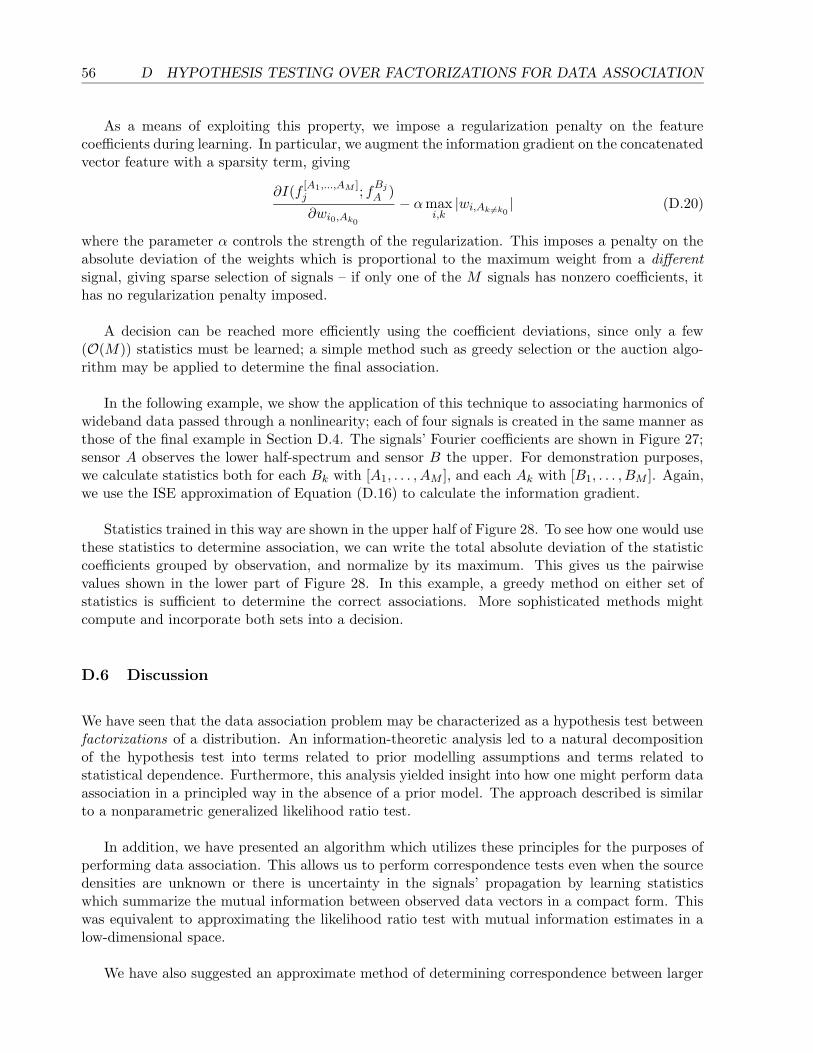
56 D HYPOTHESIS TESTING OVER FACTORIZATIONS FOR DATA ASSOCIATION
As a means of exploiting this property, we impose a regularization penalty on the featurecoefficients during learning. In particular, we augment the information gradient on the concatenatedvector feature with a sparsity term, giving
∂I(f[A1,...,AM ]j ; f
Bj
A )
∂wi0,Ak0
− αmaxi,k|wi,Ak 6=k0
| (D.20)
where the parameter α controls the strength of the regularization. This imposes a penalty on theabsolute deviation of the weights which is proportional to the maximum weight from a differentsignal, giving sparse selection of signals – if only one of the M signals has nonzero coefficients, ithas no regularization penalty imposed.
A decision can be reached more efficiently using the coefficient deviations, since only a few(O(M)) statistics must be learned; a simple method such as greedy selection or the auction algo-rithm may be applied to determine the final association.
In the following example, we show the application of this technique to associating harmonics ofwideband data passed through a nonlinearity; each of four signals is created in the same manner asthose of the final example in Section D.4. The signals’ Fourier coefficients are shown in Figure 27;sensor A observes the lower half-spectrum and sensor B the upper. For demonstration purposes,we calculate statistics both for each Bk with [A1, . . . , AM ], and each Ak with [B1, . . . , BM ]. Again,we use the ISE approximation of Equation (D.16) to calculate the information gradient.
Statistics trained in this way are shown in the upper half of Figure 28. To see how one would usethese statistics to determine association, we can write the total absolute deviation of the statisticcoefficients grouped by observation, and normalize by its maximum. This gives us the pairwisevalues shown in the lower part of Figure 28. In this example, a greedy method on either set ofstatistics is sufficient to determine the correct associations. More sophisticated methods mightcompute and incorporate both sets into a decision.
D.6 Discussion
We have seen that the data association problem may be characterized as a hypothesis test betweenfactorizations of a distribution. An information-theoretic analysis led to a natural decompositionof the hypothesis test into terms related to prior modelling assumptions and terms related tostatistical dependence. Furthermore, this analysis yielded insight into how one might perform dataassociation in a principled way in the absence of a prior model. The approach described is similarto a nonparametric generalized likelihood ratio test.
In addition, we have presented an algorithm which utilizes these principles for the purposes ofperforming data association. This allows us to perform correspondence tests even when the sourcedensities are unknown or there is uncertainty in the signals’ propagation by learning statisticswhich summarize the mutual information between observed data vectors in a compact form. Thiswas equivalent to approximating the likelihood ratio test with mutual information estimates in alow-dimensional space.
We have also suggested an approximate method of determining correspondence between larger
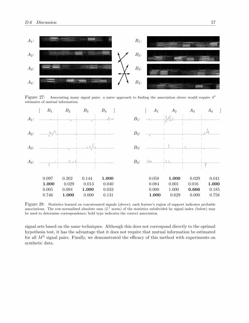
D.6 Discussion 57
A1: B1:
A2: B2:
A3: B3:
A4: N
M �
-��
� B4:
Figure 27: Associating many signal pairs: a naive approach to finding the association above would require 42
estimates of mutual information.
[ B1 B2 B3 B4 ] [ A1 A2 A3 A4 ]
A1: B1:
A2: B2:
A3: B3:
A4: B4:
0.097 0.202 0.144 1.000 0.058 1.000 0.029 0.0411.000 0.029 0.013 0.040 0.084 0.001 0.016 1.0000.005 0.094 1.000 0.033 0.000 1.000 0.666 0.1850.746 1.000 0.000 0.131 1.000 0.629 0.000 0.758
Figure 28: Statistics learned on concatenated signals (above); each feature’s region of support indicates probableassociations. The row-normalized absolute sum (L1 norm) of the statistics subdivided by signal index (below) maybe used to determine correspondence; bold type indicates the correct association
signal sets based on the same techniques. Although this does not correspond directly to the optimalhypothesis test, it has the advantage that it does not require that mutual information be estimatedfor all M2 signal pairs. Finally, we demonstrated the efficacy of this method with experiments onsynthetic data.

58 REFERENCES
References
[1] Ibrahim A. Ahmad and Pi-Erh Lin. A nonparametric estimation of the entropy for absolutelycontinuous distributions. IEEE Transactions on Information Theory, 22(3):372–375, May1976.
[2] D. L. Alspach and H.W. Sorenson. Nonlinear bayesian estimation using gaussian sum approx-imations. IEEE Transactions on Automatic Control, 17(4):439–447, August 1972.
[3] Allen Kardec Barros and Andrzej Cichocki. Extraction of specific signals with temporal struc-ture. Neural Computation, 13(9):1995–2000, September 2001.
[4] J. Beirlant, E. J. Dudewicz, L. Gyorfi, and E. C. van der Meulen. Nonparametric entropyestimation: An overview. International Journal of Math. Stat. Sci., 6(1):17–39, June 1997.
[5] Anthony J. Bell and Terrence J. Sejnowski. An information-maximization approach to blindseparation and blind deconvolution. Neural Computation, 7(6):1129–1159, 1995.
[6] C. Bishop. Neural Networks for Pattern Recognition. Clarendon Press, 1995.
[7] P. Clifford. Markov random fields in statistics. In G. R. Grimmett and D. J. A. Welsh, editors,Disorder in Physical Systems, pages 19–32. Oxford University Press, Oxford, 1990.
[8] G. Cooper. The computational complexity of probabilistic inference using Bayesian beliefnetworks. Artificial Intelligence, 42:393–405, 1990.
[9] James M. Coughlan and Sabino J. Ferreira. Finding deformable shapes using loopy beliefpropagation. In European Conference on Computer Vision 7, Copenhagen, Denmark, May2002.
[10] T. Cover and J. Thomas. Elements of Information Theory. John Wiley & Sons, New York,1991.
[11] A. P. Dawid, U. Kjærulff, and S. L. Lauritzen. Hybrid propagation in junction trees. In Adv.Intell. Comp., pages 87–97, 1995.
[12] F. De la Torre and M. J. Black. Robust parameterized component analysis: Theory andapplications to 2D facial modeling. In European Conference on Computer Vision, pages 653–669, 2002.
[13] A. Doucet, N. de Freitas, and N. Gordon, editors. Sequential Monte Carlo Methods in Practice.Springer-Verlag, New York, 2001.
[14] J.W. Fisher III, A. T. Ihler, and P. Viola. Learning informative statistics: A nonparametricapproach. In S. A. Solla, T. K. Leen, and K-R. Muller, editors, Neural Information ProcessingSystems 12, 1999.
[15] J.W. Fisher III and J.C. Principe. A methodology for information theoretic feature extraction.In A. Stuberud, editor, International Joint Conference on Neural Networks, pages ?–?, 1998.
[16] W. T. Freeman, E. C. Pasztor, and O. T. Carmichael. Learning low-level vision. InternationalJournal of Computer Vision, 40(1):25–47, 2000.

REFERENCES 59
[17] B. J. Frey, R. Koetter, and N. Petrovic. Very loopy belief propagation for unwrapping phaseimages. In Neural Information Processing Systems 14. MIT Press, 2002.
[18] S. Geman and D. Geman. Stochastic relaxation, Gibbs distributions, and the Bayesian restora-tion of images. IEEE Transactions on Pattern Analysis and Machine Intelligence, 6(6):721–741, November 1984.
[19] N. J. Gordon, D. J. Salmond, and A. F. M. Smith. Novel approach to nonlinear/non-gaussianbayesian state estimation. IEE Proceedings on Radar and Signal Processing, 140:107–113,1993.
[20] Peter Hall, Simon J. Sheather, M. C. Jones, and J. S. Marron. On optimal data-based band-width selection in kernel density estimation. Biometrika, 78(2):263–269, June 1991.
[21] David Harel. On visual formalisms. Communications of the ACM, 31(5):514–530, May 1988.
[22] A. Ihler. Maximally informative subspaces: Nonparametric estimation for dynamical systems.Master’s thesis, MIT, December 2000.
[23] A. Ihler, J. Fisher, and A. S. Willsky. Nonparametric estimators for online signature au-thentication. In International Conference on Acoustics, Speech, and Signal Processing, May2001.
[24] A. Ihler, J. Fisher, and A. S. Willsky. Hypothesis testing over factorizations for data associa-tion. In Information Processing in Sensor Networks, April 2003.
[25] A. T. Ihler, E. B. Sudderth, W. T. Freeman, and A. S. Willsky. Efficient multiscale samplingfrom products of gaussian mixtures. In Neural Information Processing Systems 17, 2003.
[26] M. Isard and A. Blake. Contour tracking by stochastic propagation of conditional density. InECCV, pages 343–356, 1996.
[27] M. Isard and A. Blake. Condensation – conditional density propagation for visual tracking.International Journal of Computer Vision, 29(1):5–28, 1998.
[28] M. Isard and A. Blake. A smoothing filter for condensation. In European Conference onComputer Vision, pages 767–781, 1998.
[29] Harry Joe. Estimation of entropy and other functionals of a multivariate density. Annals ofthe Institute of Statistical Mathematics, 41(4):683–697, 1989.
[30] T. Kailath, A. H. Sayed, and B. Hassibi. Linear Estimation. Information and System Sciences.Prentice Hall, New Jersey, 2000.
[31] E. J. Kelly. An adaptive detection algorithm. IEEE Transactions on Aerospace and ElectricalSystems, 22(1):115–127, 1986.
[32] D. Koller, U. Lerner, and D. Angelov. A general algorithm for approximate inference and itsapplication to hybrid Bayes nets. In Uncertainty in Artificial Intelligence 15, pages 324–333,1999.
[33] S. Kullback and R. A. Leibler. On information and sufficiency. Annals of MathematicalStatistics, 22:79–86, 1951.

60 REFERENCES
[34] S. L. Lauritzen. Graphical Models. Oxford University Press, Oxford, 1996.
[35] Te-Won Lee. Nonlinear approaches to independent component analysis. In American Instituteof Physics, October 1999.
[36] A. M. Martınez and R. Benavente. The AR face database. Technical Report 24, CVC, June1998.
[37] B. Moghaddam and A. Pentland. Probabilistic visual learning for object representation. IEEETransactions on Pattern Analysis and Machine Intelligence, 19(7):696–710, July 1997.
[38] R. Moses and R. Patterson. Self-calibration of sensor networks. In SPIE vol. 4743: UnattendedGround Sensor Technologies and Applications IV, 2002.
[39] O. Nestares and D. J. Fleet. Probabilistic tracking of motion boundaries with spatiotemporalpredictions. In CVPR, pages 358–365, 2001.
[40] E. Parzen. On estimation of a probability density function and mode. Annals of MathematicalStatistics, 33:1065–1076, 1962.
[41] J. Pearl. Probabilistic Reasoning in Intelligent Systems. Morgan Kaufman, San Mateo, 1988.
[42] Barak Pearlmutter and Lucas Parra. A contex-sensitive generalization of ica. In InternationalConference on Neural Information Processing, Hong Kong, September 1996.
[43] R. Plamondon and S. Srihari. On-line and off-line handwriting recognition: A comprehensivesurvey. IEEE Transactions on Pattern Analysis and Machine Intelligence, 22(1):63–84, 2000.
[44] Robert F. Popoli and Jerry M. Mendel. Relative sufficiency. IEEE Transactions on AutomaticControl, 38(5):826–828, May 1993.
[45] S. J. Sheather and M. C. Jones. A reliable data-based bandwidth selection method for kerneldensity estimation. Journal of Royal Statistical Society, Series B, 53(3):683–690, 1991.
[46] H. Sidenbladh and M. J. Black. Learning the statistics of people in images and video. Inter-national Journal of Computer Vision, 2003. To appear.
[47] B.W. Silverman. Density Estimation for Statistics and Data Analysis. Chapman and Hall,New York, 1986.
[48] E. B. Sudderth, A. T. Ihler, W. T. Freeman, and A. S. Willsky. Nonparametric belief propaga-tion. Technical Report 2551, MIT Laboratory for Information and Decision Systems, October2002.
[49] E. B. Sudderth, A. T. Ihler, W. T. Freeman, and A. S. Willsky. Nonparametric belief propa-gation. In IEEE Computer Vision and Pattern Recognition, 2003.
[50] J. Sun, H. Shum, and N. Zheng. Stereo matching using belief propagation. In A. et al. Heyden,editor, European Conference on Computer Vision, pages 510–524. Springer-Verlag, 2002.
[51] M. J. Wainwright, T. Jaakkola, and A. S. Willsky. Tree–based reparameterization for approx-imate inference on loopy graphs. In Neural Information Processing Systems 14. MIT Press,2002.

REFERENCES 61
[52] M. Weber, M. Welling, and P. Perona. Unsupervised learning of models for recognition. InECCV, pages 18–32, 2000.
[53] Y. Weiss and W. T. Freeman. On the optimality of solutions of the Max–Product Belief–Propagation algorithm in arbitrary graphs. IEEE Transactions on Information Theory,47(2):736–744, February 2001.
[54] Yair Weiss. Deriving intrinsic images from image sequences. In International Conference onComputer Vision, pages 68–75, 2001.
[55] J. S. Yedidia, W. T. Freeman, and Y. Weiss. Understanding belief propagation and its gener-alizations. In International Joint Conference on Artificial Intelligence, August 2001.
[56] J. S. Yedidia, W. T. Freeman, and Y. Weiss. Constructing free energy approximations andgeneralized belief propagation algorithms. Technical Report 2002-35, MERL, August 2002.