Mass transfer and mergers in double white dwarf binaries

Louisiana State UniversityLSU Digital Commons

LSU Doctoral Dissertations Graduate School

2010

Mass transfer and mergers in double white dwarfbinariesWesley Paul EvenLouisiana State University and Agricultural and Mechanical College, [email protected]

Follow this and additional works at: https://digitalcommons.lsu.edu/gradschool_dissertations

Part of the Physical Sciences and Mathematics Commons

This Dissertation is brought to you for free and open access by the Graduate School at LSU Digital Commons. It has been accepted for inclusion inLSU Doctoral Dissertations by an authorized graduate school editor of LSU Digital Commons. For more information, please [email protected].

Recommended CitationEven, Wesley Paul, "Mass transfer and mergers in double white dwarf binaries" (2010). LSU Doctoral Dissertations. 3436.https://digitalcommons.lsu.edu/gradschool_dissertations/3436

https://digitalcommons.lsu.edu?utm_source=digitalcommons.lsu.edu%2Fgradschool_dissertations%2F3436&utm_medium=PDF&utm_campaign=PDFCoverPages

https://digitalcommons.lsu.edu/gradschool_dissertations?utm_source=digitalcommons.lsu.edu%2Fgradschool_dissertations%2F3436&utm_medium=PDF&utm_campaign=PDFCoverPages

https://digitalcommons.lsu.edu/gradschool?utm_source=digitalcommons.lsu.edu%2Fgradschool_dissertations%2F3436&utm_medium=PDF&utm_campaign=PDFCoverPages

https://digitalcommons.lsu.edu/gradschool_dissertations?utm_source=digitalcommons.lsu.edu%2Fgradschool_dissertations%2F3436&utm_medium=PDF&utm_campaign=PDFCoverPages

http://network.bepress.com/hgg/discipline/114?utm_source=digitalcommons.lsu.edu%2Fgradschool_dissertations%2F3436&utm_medium=PDF&utm_campaign=PDFCoverPages

https://digitalcommons.lsu.edu/gradschool_dissertations/3436?utm_source=digitalcommons.lsu.edu%2Fgradschool_dissertations%2F3436&utm_medium=PDF&utm_campaign=PDFCoverPages

mailto:[email protected]

MASS TRANSFER AND MERGERS IN DOUBLE WHITE DWARF BINARIES.

A Dissertation

Submitted to the Graduate Faculty of theLouisiana State University and

Agricultural and Mechanical Collegein partial fulfillment of the

requirements for the degree ofDoctor of Philosophy

in

The Department of Physics and Astronomy

byWesley Paul Even

B.S., University of Northern Iowa, 2003M.S., Louisiana State University, 2008

May, 2010

Dedication

For my parents, Eugene and Paula...

ii

Acknowledgments

I would like to thank my adviser Joel Tohline for his support, guidance, and infinite patience

throughout this research and my time at LSU. I would also like to thank Juhan Frank for

his questions and insights, making sure that I considered the physics and didn’t get lost

in the computational aspects of this research. In addition, thank you to astronomy faculty

members Geoff Clayton, Brad Schaeffer, Robert Hynes, and Arlo Landolt.

I would like to thank postdoctoral researchers Patrick Motl and Shangli Ou for intro-

ducing me to the codes and other computational tools that were required to conduct this

research. I would also like to thank my colleagues, especially Robert Beaird, Charles Bradley,

Jay Call, Andrew Collazzi, Sulakshana Thanvanthri, and Sai Vinjanampathy for their com-

panionship and support throughout graduate school. I would also like to thank the professors

and students in the IGERT on Computational Fluid Dynamics for exposing me to new fields

and different ways of looking at my research, in particular my IGERT adviser Blaise Bourdin

and my fellow students Luis Alvergue, Michael Crochet, Farid Harhad, Tyler Landis, and

Kevin Tubbs.

I would like to thank the physics professors at the University of Northern Iowa who

introduced me to physics, especially Michael Roth for initiating my computational physics

research. Finally, I would like to thank my family for all their support and encouragement

as I have pursued my dreams.

This work has been supported in part, by grants AST-0708551 and DGE-0504507 from the

U.S. National Science Foundation and, in part, by grants NNX07AG84G and NNX10AC72G

from NASA’s Astrophysics Theory Program. This research also has been made possible by

grants of high-performance computing time on the TeraGrid (MCA98N043), at LSU, and

across LONI (Louisiana Optical Network Initiative).

iii

Table of Contents

Dedication . . . . . . . . . . . . . . . . . . . . . . . . . . . . . . . . . . . . . . . . . ii

Acknowledgments . . . . . . . . . . . . . . . . . . . . . . . . . . . . . . . . . . . . . iii

List of Tables . . . . . . . . . . . . . . . . . . . . . . . . . . . . . . . . . . . . . . . . vi

List of Figures . . . . . . . . . . . . . . . . . . . . . . . . . . . . . . . . . . . . . . . vii

Abstract . . . . . . . . . . . . . . . . . . . . . . . . . . . . . . . . . . . . . . . . . . ix

1. Introduction . . . . . . . . . . . . . . . . . . . . . . . . . . . . . . . . . . . . . . . 11.1 White Dwarfs . . . . . . . . . . . . . . . . . . . . . . . . . . . . . . . . . . . 11.2 Binary Stars . . . . . . . . . . . . . . . . . . . . . . . . . . . . . . . . . . . . 21.3 Double White Dwarfs . . . . . . . . . . . . . . . . . . . . . . . . . . . . . . . 61.4 Supernovae . . . . . . . . . . . . . . . . . . . . . . . . . . . . . . . . . . . . 71.5 Previous Double White Dwarf Simulations . . . . . . . . . . . . . . . . . . . 81.6 This Work . . . . . . . . . . . . . . . . . . . . . . . . . . . . . . . . . . . . . 9

2. Self Consistent Field Technique . . . . . . . . . . . . . . . . . . . . . . . . . . . . 112.1 Zero Temperature Equation of State . . . . . . . . . . . . . . . . . . . . . . 112.2 Numerical Solutions for the Gravitational Potential . . . . . . . . . . . . . . 25

3. Steady State Binary Sequences . . . . . . . . . . . . . . . . . . . . . . . . . . . . 313.1 Inspiral White Dwarf Binary Sequences . . . . . . . . . . . . . . . . . . . . 343.2 Contact Sequences . . . . . . . . . . . . . . . . . . . . . . . . . . . . . . . . 52

4. Hydrodynamic Techniques . . . . . . . . . . . . . . . . . . . . . . . . . . . . . . . 614.1 Summary of Hydrodynamics Code . . . . . . . . . . . . . . . . . . . . . . . . 624.2 Zero Temperature Equation of State . . . . . . . . . . . . . . . . . . . . . . 63

5. Binary Merger Simulations . . . . . . . . . . . . . . . . . . . . . . . . . . . . . . . 715.1 Previously Published Hydrocode Simulations . . . . . . . . . . . . . . . . . . 715.2 q = 0.7 Polytrope . . . . . . . . . . . . . . . . . . . . . . . . . . . . . . . . . 725.3 q = 2/3 Zero Temperature . . . . . . . . . . . . . . . . . . . . . . . . . . . . 735.4 q = 2/3 Zero Temperature Plus Ideal Gas . . . . . . . . . . . . . . . . . . . 81

6. Conclusions . . . . . . . . . . . . . . . . . . . . . . . . . . . . . . . . . . . . . . . 104

Bibliography . . . . . . . . . . . . . . . . . . . . . . . . . . . . . . . . . . . . . . . . 107

Appendix A White Dwarf Mass-Radius Relationship . . . . . . . . . . . . . . . . . . 109

Appendix B Physical Constants . . . . . . . . . . . . . . . . . . . . . . . . . . . . . 112

Appendix C List of Variables . . . . . . . . . . . . . . . . . . . . . . . . . . . . . . . 114

iv

Appendix D Letter of Permission . . . . . . . . . . . . . . . . . . . . . . . . . . . . . 117

Vita . . . . . . . . . . . . . . . . . . . . . . . . . . . . . . . . . . . . . . . . . . . . . 118

v

List of Tables

2.1 Convergence of SCF Method . . . . . . . . . . . . . . . . . . . . . . . . . . . 23

2.2 Error of Poisson Solver for Spherical Polytropes . . . . . . . . . . . . . . . . 30

3.1 Sequence of single, nonrotating ZTWDs . . . . . . . . . . . . . . . . . . . . . 32

3.2 Selected single, nonrotating ZTWDs . . . . . . . . . . . . . . . . . . . . . . 35

3.3 DWD Inspiral Sequence ‘A’:Mtot = 1.5M⊙; q=1 . . . . . . . . . . . . . . . . 36

3.4 Individual Stellar Components along DWD Inspiral Sequence ‘A’ . . . . . . . 37

3.5 DWD Inspiral Sequence ‘B’:Mtot = 1.5M⊙; q = 2/3 . . . . . . . . . . . . . . 39

3.6 Individual Stellar Components along DWD Inspiral Sequence ‘B’ . . . . . . . 41

3.7 DWD Inspiral Sequence ‘C’:Mtot = 1.5M⊙; q = 1/2 . . . . . . . . . . . . . . 43

3.8 Individual Stellar Components along DWD Inspiral Sequence ‘C’ . . . . . . . 44

3.9 Semi-detached DWD Sequence ‘D’; Mtot = 1.5M⊙ . . . . . . . . . . . . . . . 53

3.10 Semi-detached DWD Sequence ‘E’; Mtot = 1.0M⊙ . . . . . . . . . . . . . . . 54

4.1 Variation of timestep size with ρp/ρ∗ . . . . . . . . . . . . . . . . . . . . . . 68

B.1 Physical Constants . . . . . . . . . . . . . . . . . . . . . . . . . . . . . . . . 113

C.1 List of Variables . . . . . . . . . . . . . . . . . . . . . . . . . . . . . . . . . . 115

vi

List of Figures

1.1 Properties of Single Non-rotating White Dwarfs . . . . . . . . . . . . . . . . . . 3

1.2 Effective Gravitational Potential for a Binary System . . . . . . . . . . . . . . . 5

2.1 Schematic Diagram of the Structure of a Binary System . . . . . . . . . . . . . 14

2.2 Solutions and Errors for Poisson Solver . . . . . . . . . . . . . . . . . . . . . . . 29

3.1 Mass-Radius Relation for White Dwarfs . . . . . . . . . . . . . . . . . . . . . . 33

3.2 Density Contours for q=1 White Dwarf Binaries . . . . . . . . . . . . . . . . . . 46

3.3 Density Contours for q=2/3 White Dwarf Binaries . . . . . . . . . . . . . . . . 47

3.4 Density Contours for q=1/2 White Dwarf Binaries . . . . . . . . . . . . . . . . 48

3.5 Sequence of q=1 White Dwarf Binaries as a Function of Separation . . . . . . . 56

3.6 Sequence of q=2/3 White Dwarf Binaries as a Function of Separation . . . . . . 57

3.7 Sequence of q=1/2 White Dwarf Binaries as a Function of Separation . . . . . . 58

3.8 Sequence of Mtot = 1.5M⊙ White Dwarf Binaries as a Function of Mass Ratio . 59

3.9 Sequence of Mtot = 1.0M⊙ White Dwarf Binaries as a Function of Mass Ratio . 60

4.1 Comparison of Separation for Different Values of ρp/ρ∗ . . . . . . . . . . . . . . 68

4.2 Comparison of Time Variation of Momentum and the Central Density for Differ-ent Values of ρp/ρ∗ . . . . . . . . . . . . . . . . . . . . . . . . . . . . . . . . 69

4.3 Density and Pressure Contours for Different Values of ρp/ρ∗ . . . . . . . . . . . 70

5.1 Density Contours for a Q0.7a Polytropic Binary Merger Simulation . . . . . . . 74

5.2 Mass vs. Time for a q=0.7 Polytropic Binary Simulation . . . . . . . . . . . . . 75

5.3 Binary Separation and Angular Momentum vs. Time for a q=0.7 PolytropicBinary Simulation . . . . . . . . . . . . . . . . . . . . . . . . . . . . . . . . . 76

5.4 Angular Momentum Components vs. Time for a q=0.7 Polytropic Binary Simu-lation . . . . . . . . . . . . . . . . . . . . . . . . . . . . . . . . . . . . . . . . 77

5.5 Time Rate of Change of Mass for a q=0.7 Polytropic Binary Simulation . . . . . 78

vii

5.6 Density Contours for a q=2/3 DWD Binary Merger Simulation with a ZTWD EOS 87

5.7 Azimuthally Averaged Density in the Equatorial plane for the Final Object in aq=2/3 DWD Binary Merger with a ZTWD EOS . . . . . . . . . . . . . . . . 88

5.8 Azimuthally Averaged Density for the Final Object in a q=2/3 DWD BinaryMerger with a ZTWD EOS . . . . . . . . . . . . . . . . . . . . . . . . . . . 88

5.9 Angular Velocity as a Function of the Keplerian Velocity for the Final Object ina q=2/3 DWD Binary Merger with a ZTWD EOS . . . . . . . . . . . . . . . 89

5.10 Density and Temperature Contours for a q=2/3 DWD Binary Merger with aZTWD Plus Ideal Gas EOS . . . . . . . . . . . . . . . . . . . . . . . . . . . 90

5.11 Density and Temperature Contours for a q=2/3 DWD Binary Merger with aZTWD Plus Ideal Gas EOS . . . . . . . . . . . . . . . . . . . . . . . . . . . 91

5.12 Mass vs. Time for 2 q=2/3 DWD Binary Simulations with Different EOS . . . . 92

5.13 Separation and Angular Momentum vs. Time for 2 q=2/3 DWD Binary Simula-tions with Different EOS . . . . . . . . . . . . . . . . . . . . . . . . . . . . . 93

5.14 Angular Momentum Components vs. Time for 2 q=2/3 DWD Binary Simulationswith Different EOS . . . . . . . . . . . . . . . . . . . . . . . . . . . . . . . . 94

5.15 Central Density vs. Time for 2 q=2/3 DWD Binary Simulations with DifferentEOS . . . . . . . . . . . . . . . . . . . . . . . . . . . . . . . . . . . . . . . . 95

5.16 Time Rate of Change of Mass vs. Time for 2 q=2/3 DWD Binary Simulationswith Different EOS . . . . . . . . . . . . . . . . . . . . . . . . . . . . . . . . 96

5.17 Azimuthally Averaged Density for the Final Object in a q=2/3 DWD BinaryMerger with a ZTWD Plus Ideal Gas EOS . . . . . . . . . . . . . . . . . . . 97

5.18 Angular Velocity as a Function of the Keplerian Velocity for the Final Object ina q=2/3 DWD Binary Merger with a ZTWD Plus Ideal Gas EOS . . . . . . 98

5.19 Azimuthally Averaged Density in the Equatorial Plane for the Final Object in aq=2/3 DWD Binary Merger with a ZTWD Plus Ideal Gas EOS . . . . . . . 99

5.20 Azimuthally Averaged Temperature in the Equatorial Plane for the Final Objectin a q=2/3 DWD Binary Merger with a ZTWD Plus Ideal Gas EOS . . . . . 100

5.21 Maximum Temperature for a Density Contour as a Function of Time . . . . . . 101

5.22 Nuclear Energy Generation Rates at 12.5 Orbits into a q=2/3 WD Binary Mergerwith a ZTWD Plus Ideal Gas EOS . . . . . . . . . . . . . . . . . . . . . . . 102

viii

5.23 Nuclear Energy Generation Rates at 22.0 Orbits into a q=2/3 WD Binary Mergerwith a ZTWD Plus Ideal Gas EOS . . . . . . . . . . . . . . . . . . . . . . . 103

ix

Abstract

We have developed a self consistent field (SCF) technique similar to the one described by

Hachisu, Eriguchi, & Nomoto (1986b) that can be used to construct detailed force-balanced

models of synchronously rotating, double white dwarf (DWD) binaries. This SCF technique

can be used to construct model sequences that mimic the last portion of the detached inspiral

phase of DWD binary evolutions, and semi-detached model sequences that mimic a phase of

conservative mass transfer. In addition, the SCF models can be used to provide quiet initial

starts for dynamical studies of the onset of mass transfer in DWD systems. We present

multiple dynamical simulations of interacting DWD binaries using these improved initial

models and a modified version of the hydrodynamics code developed originally by Motl et

al. (2002) to investigate the stability of mass transfer and the possibility that DWD binary

mergers serve as progenitors for Type Ia supernovae. These are among the first white dwarf

merger simulations carried out using a grid-based hydrodynamics technique and a realistic

equation of state. Where there is overlap, our results compare favorably to simulations

that have been previously published by other groups but carried out using smooth particle

hydrodynamics (SPH) techniques.

x

1. Introduction

1.1 White Dwarfs

Energy in main sequence stars, like the sun, is generated from fusion occurring in the core of

the star. Main sequence stars initially fuse hydrogen into helium. If a star has enough mass

it can eventually form a region where helium is fused to form carbon and oxygen. Depending

on the mass of the star this fusion process can create elements up to iron. For elements with

an atomic number greater than iron the fusion process absorbs thermal energy and reduces

the pressure support in the interior of the star, causing the core to collapse under the force

of gravity. During the burning of elements between He and Fe the outer layers of a star can

expand radially and develop instabilities. This can lead to the outer layers being ejected

from the star and leaving only the dense core of heavy material behind. This exposed core

is no longer undergoing fusion and is called a white dwarf. Since this core was formerly the

central fusion engine of the star it will be extremely hot, but also very small in size compared

to a main sequence star. Typical white dwarfs have approximately the same radius as the

Earth, but a mass comparable to the sun’s mass. Due to this small size white dwarfs have

very low luminosity despite there high temperature. The first optically resolved white dwarf,

Sirus B, was seen by Alvan Clark in 1862.

The extreme densities obtained from the calculation of mass and radius from white dwarf

observations indicate that white dwarfs can not be made of an ordinary gas. After fusion

in the core ends the star will begin to contract because the nuclear reactions that were

previously imparting energy into the star have stopped and there is no source of energy

to prevent gravitational collapse. As the ionized gas compresses the electrons become so

tightly packed that quantum effects begin to play a dominate role in the structure. The

1

2

Pauli exclusion principle disallows two electrons from occupying the same quantum state

and in atoms this leads to the electron shell structure. In the white dwarf the exclusion

principle creates a pressure as electrons require more energy to occupy the same volumes.

Even if the normal agitation of the gas is ignored - that is, even if the normal gas temperature

is set to zero - this degeneracy pressure can become great enough to stop the gravitational

collapse and create a stable star.

Figure 1.1 graphs several relationships for “zero-temperature” white dwarfs (ZTWDs).

These are calculated using a simplified 1D version of the self consistent field code described

in Chapter 2. Two physical characteristics about white dwarfs can be easily seen from these

figures: the size of the white dwarf decreases as the mass increases; and there is a maximum

mass for white dwarfs. The reasons for this will be discussed more in §2.1.

1.2 Binary Stars

Sirius B is in a binary system with a main sequence star Sirius A, the brightest star in the

night sky. Binary systems occur when 2 stars form close enough together that they are

gravitationally bound and the two stars orbit around the center of mass of the system. The

existence of binary stars has been known to astronomers for over 300 years. Binary systems

are very common with over half of all stars being in a binary system. Binary systems allow

insight into parameters that are not obtainable by observations of single stars. In particular,

the masses of stars can be calculated if there are multiple stars in a system using Kepler’s

laws. Most binary stars interact almost exclusively through gravitational forces. However,

systems can evolve to a point where matter from one star can interact directly with the other

star in the system. This can occur for example, if there are strong winds off one star or if

one star overfills its so called Roche lobe.

The Roche potential is the effective potential of a binary system in a circular orbit as

3

Figure 1.1 Properties of a series of single isolated non-rotating zero temperature white dwarfs.Upper left: Mass as a function of the central density. Upper right: Mass radius of gyration asa function of central density. The n=3/2 and n=3 lines represent the values for a polytropicstar with a polytropic index of 3/2 and 3 respectively. Lower left: Radius as a function ofcentral density. Lower right: Radius as a function of mass.

4

viewed from a frame rotating with the system’s orbital frequency Ω. The equation for the

Roche potential, ΦR, for point mass stars is given by,

ΦR(~r) = −GM1

|~r − ~r1|−

GM2

|~r − ~r2|−

1

2Ω22, (1.1)

where ~r is the position at which the potential is being evaluated, ~r1 is the location of the

first star, ~r2 is the location of the second star, is the distance from the orbital axis of the

binary system to the position ~r, G is the gravitational constant, and M1 and M2 are the

masses of the respective stars.

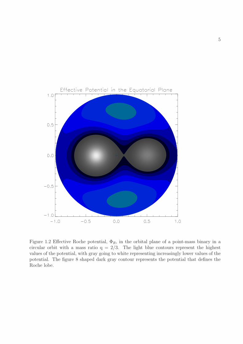
In Figure 1.2 equipotential contours are drawn in the equatorial plane of the binary; the

final grey contour creates a figure eight shape. The volume inside this contour is known as

the Roche lobe. The point of intersection of this contour has been named the first Lagrange

point (L1). The L1 point is a saddle equilibrium point in the potential. Matter at this point

is equally bound to both stars. If a star grows larger than its Roche lobe then it will begin

to transfer mass to its companion through the L1 point.

Binary systems can be separated into three different classes based on the Roche potential.

A detached system is a binary where neither star is filling its respective Roche lobe. In a

semi-detached system one star (the donor) is filling it Roche lobe and transferring material

to its companion (the accretor), which is not filling its Roche lobe. Contact binaries are

systems where both stars have filled their Roche lobe; these can be further classified as

over-contact if the stars are significantly overfilling their Roche lobe.

Stars can fill their Roche lobe through two different mechanisms: the star increases its

size due to physical changes within the star, or the separation between the stars decreases,

thereby reducing the size of the Roche lobe.

For main sequence stars the likely scenario for coming into contact/semi-contact is that

one of the stars increases its radius to fill the Roche Lobe. This occurs when the donor

leaves the main sequence and evolves onto the giant branch. Since more massive stars evolve

5

Figure 1.2 Effective Roche potential, ΦR, in the orbital plane of a point-mass binary in acircular orbit with a mass ratio q = 2/3. The light blue contours represent the highestvalues of the potential, with gray going to white representing increasingly lower values of thepotential. The figure 8 shaped dark gray contour represents the potential that defines theRoche lobe.

6

faster, the donor will be the more massive of the two stars. Eventually the outer layers of

the donor can be ejected from the star, leaving behind a binary system with a main sequence

star and a white dwarf. This system will no longer have Roche lobe overflow since the donor

has had to decrease greatly in size to become a white dwarf, and the system will return

to being a detached binary. Eventually the remaining main sequence star can also evolve

to the giant branch and overflow its Roche lobe and become the new donor. During this

phase material will be transfered onto the white dwarf. This class of systems is known as

cataclysmic variables (CVs). After further evolution the outer layers of the new donor can

be removed and a Double White Dwarf (DWD) binary system will remain.

1.3 Double White Dwarfs

Even detached DWD binaries can eventually come into contact as their separation is reduced

due to the loss of angular momentum due to gravitational radiation. AM CVn systems

are observed binary systems that have orbital periods of less than an hour and are blue

when observed at optical wavelengths. They are also observed to be varying in brightness

(Nelemans et al.2001). Based on their short periods and other observational evidence it is

widely believed that AM CVn systems are semi-detached DWD binaries. The systems are

theorized to have formed as detached systems that have been brought into mass transfer

through gravitational wave radiation removing angular momentum from the system. There

are currently 17 confirmed AM CVn systems and 2 candidate systems (Ramsey et al. 2007).

While this is a relatively small number of observed systems, the number of AM CVn system

in the Galaxy is calculated to be approximately 107.

7

1.4 Supernovae

Supernovae are among the most luminous astronomical events observed in the optical spec-

trum. Supernovae have been divided into different classifications based on their observed

spectra. Type Ia supernovae have been observed to have a very predictable light curve

where the decay time is strongly correlated to the maximum brightness. This makes Type

Ia supernovae an excellent standard candle for determining distances. Currently there are

several proposals for the progenitor systems to Type Ia supernovae. Type Ia lack hydrogen

lines in there spectrum and have been observed in both young and old stellar populations

where no star formation is occurring. White dwarfs will be extremely hydrogen deficient and

be present in older stellar populations, but if they are isolated stars there is no mechanism

available to cause them to explode and release the vast amount of energy seen in supernovae.

The leading theories for Type Ia supernovae all involve a white dwarf in a binary system.

However, there is no consensus on the nature of the donor star or the chemical composition

of the white dwarf (Livio 2000). The possible systems can be divided into two broad classes:

double degenerate systems and single degenerate systems. In the double degenerate scenario

an AM CVn system would be formed with a total mass over the Chandrasekhar mass. The

Chandrasekhar mass limit, MCh, is the mass at which the electron degeneracy pressure can no

longer support the star and it begins collapse due to its own gravity; for a non-rotating white

dwarf this mass is approximately 1.44 M⊙ (see the bottom, right-hand panel of Figure 1.1).

Eventually the accretor would gain enough mass that it crosses the Chandrasekhar mass

limit, either through steady accretion or rapid merger. At this point the accretor would

begin to collapse. Before it collapses, rapid fusion would begin, releasing large amounts of

energy. In the single degenerate case the donor would be a non-degenerate star that transfers

hydrogen rich material onto the surface of the white dwarf accretor at a rate high enough to

maintain steady hydrogen burning on the surface of the white dwarf. Eventually the accretor

8

accretes enough mass and crosses the Chandrasekhar limit resulting in a rapid fusion event

as in the double degenerate case.

1.5 Previous Double White Dwarf Simulations

In an effort to understand possible progenitors of Type Ia SNe, a number of simulations

of DWD binary mergers have been conducted by various groups over the last two decades.

All previous simulations have been conducted using a numerical technique referred to as

smoothed particle hydrodynamics (SPH). The simulations have been improved over this

period with better numerical methods, more physics, and an increased number of simulation

particles. However, the qualitative result of the merger has remained largely constant.

Benz et al. (1989) simulated the merger of a 0.9 M⊙ and a 1.2 M⊙ DWD system.

The simulation was conducted using 7000 smoothed particles and non-rotating spherical

white dwarfs as the initial conditions. The donor was quickly disrupted and the system

merged in approximately 2.5 orbital periods. The final product of the merger was a rotating

degenerate core composed mostly of material from the accretor that is surrounded by a hot

semi-degenerate envelope and a non-degenerate disk.

Segretain et al. (1997) investigated the merger of a 0.6 M⊙ and a 0.9 M⊙ DWD binary

system. Again, the initial model for the simulation was constructed by placing two non-

rotating spherically symmetric stars in orbit about each other, with the donor over filling its

Roche lobe. The simulation was carried out at two different resolutions: 7288 and 58,304

particles. Both simulations produced similar results. The result of the merger was an

unheated uniformly rotating degenerate core surrounded by a shock heated layer. This was

surrounded by an envelope of material, consisting mostly of matter from the donor. This was

the hottest region in the merger and the most likely location for fusion to occur. Additionally,

a rotationally supported low density disk of material forms around the merged white dwarf.

Guerrero et al. (2004) investigated 6 different binary systems ranging from a 0.4 M⊙ and

9

0.4M⊙ system to a 0.8 M⊙ and 1.0 M⊙ pair. The paper focuses most of its attention on the

merger of a 0.6 M⊙ white dwarf with a 0.8 M⊙ white dwarf. The simulations were begun

with neither star initially filling its Roche lobe and a small artificial acceleration was applied

to the system until mass transfer began. Approximately 50,000 particles where used in the

simulations that produced configurations similar to those in Segretain et al. (1997). These

simulations also included a nuclear reaction network. In the merger, fusion would begin in

the shock heated region, but would quench itself and did not play a significant role in the

final outcome of the merger.

Yoon et al. (2007) investigated a DWD system with a 0.6 M⊙ donor and a 0.9 M⊙

accretor. This simulation increased the number of particles used to 200,000 and followed

the evolution for twice the time of any of the previous simulations discussed. The maximum

temperature reached in the simulation was slightly above the carbon burning temperature

of 109 K, but again the burning was limited by the expansion of the gas when heated. The

final product of this merger was a slowly rotating cold core surrounded by a rapidly rotating

elliptical envelope of hot material. A thick rotationally supported disk was also formed.

1.6 This Work

Here we investigate initial conditions that are closer to equilibrium than was done in the

simulations discussed in Section 1.5. This is done by constructing steady state equilibrium

models of synchronously rotating DWD binaries with a separation greater than acrit, the

separation at which one star begins to overflow its Roche lobe. These models are used

to mimic the gravitational inspiral of the DWD binary and are used as initial conditions

for computational fluid dynamics (CFD) simulations of mass transferring DWD systems.

As described in Chapter 4, the CFD technique used here is very different from the SPH

technique; it involves advecting fluid across a grid. Multiple CFD simulations are conducted

10

to verify our technique and to study the merger of the DWD systems as possible progenitors

to type Ia supernovae.

2. Self Consistent Field Technique1

2.1 Zero Temperature Equation of State

The Self Consistent Field (SCF) technique was first introduced to the astrophysics com-

munity by Ostriker & Mark (1964) to create models of rapidly rotating, single stars with

a polytropic equation of state. Hachisu developed a variation of the technique, improving

convergence rates and extending its capabilities to include the use of a zero temperature

white dwarf (ZTWD) equation of state. With his improved technique, Hachisu was able to

construct two-dimensional (2D) configurations of differentially rotating, single white dwarfs

(Hachisu, 1986a) and three-dimensional (3D) configurations of uniformly rotating multiple

white dwarf systems in which the stars have equal mass (Hachisu, 1986b). New & Tohline

(1997) employed Hachisu’s 3D technique to construct inspiral sequences of equal-mass DWD

binaries, including over-contact models having separations even smaller than acrit. Hachisu

(1986b) also applied his technique to the construction of unequal-mass binary systems using

a polytropic equation of state and, after additional algorithmic innovations were introduced,

Hachisu, Eriguchi, and Nomoto (1986a,b) constructed a small sample of unequal-mass DWD

binaries and heavy-disk white dwarf systems to examine the likely outcome of DWD mergers.

In what follows we show how Hachisu’s SCF technique for constructing unequal-mass DWD

binaries can be further improved and used to construct inspiral binary sequences.

1§2.1 and Chapter 3 reproduced by permission of the AAS (Even & Tohline (2009))

11

12

2.1.1 Equation of State

In the ZTWD equation of state (Chandrasekhar, 1935, 1967; Hachisu, 1986a) the electron

degeneracy pressure P varies with the mass density ρ according to the relation,

P = A[

x(2x2 − 3)(x2 + 1)1/2 + 3 sinh−1 x]

, (2.1)

where the dimensionless parameter,

x ≡(

ρ

B

)1/3

, (2.2)

and the constants A and B are (see Appendix A and Table B.1 for elaboration),

A ≡πm4

ec5

3h3= 6.00228 × 1022 dynes cm−2 , (2.3)

B

µe

≡8πmp

3

(

mec

h

)3

= 9.81011 × 105 g cm−3 . (2.4)

According to Chandrasekhar (1967) (see again our Appendix A), a natural length scale

associated with models of ZTWDs is,

µeℓ1 =(

2A

πG

)1/2 µe

B= 7.71395 × 108 cm = 0.0111R⊙ , (2.5)

and the associated limiting white dwarf mass is,

µ2eMch = 4π(2.01824)

(

2A

πG

)3/2(µe

B

)2

= 1.14205 × 1034 g = 5.742M⊙ . (2.6)

Throughout this work, we will assume that the average ratio of nucleons to electrons through-

out each white dwarf is µe = 2. Hence, B = 1.96202× 106 g cm−3, ℓ1 = 5.55× 10−3R⊙, and

Mch = 1.435M⊙.

In terms of the enthalpy of the gas,2

H ≡∫ dP

ρ, (2.7)

2As defined here, H is actually enthalpy per unit mass.

13

the ZTWD equation of state shown in Eq. (2.1) can also be written in the form,

H =8A

B

[

x2 + 1]1/2

. (2.8)

Inverting this gives the dependence of ρ on H, namely,

ρ

B= x3 =

[(

BH

8A

)2

− 1]3/2

. (2.9)

As a foundation for both constructing and understanding the structures of the syn-

chronously rotating and tidally distorted stars in ZTWD binary systems, we have regener-

ated Chandraskehar’s spherical white dwarf sequence using a variation of the SCF technique

outlined by Hachisu (1986a) and described more fully in §2.1.3 below using both a 1D and 3D

code. As is discussed in Chapter 3, Table 3.1 details key properties of the ZTWD structures

that lie along this spherical model sequence. The white dwarf mass-radius relationship that

is derived from the 3D models along this sequence is illustrated by the diamonds in Fig-

ure 3.1. For comparison, results from the published spherical sequence of Hachisu (1986a)

are represented in this figure by asterisks and the solid curve shows the approximate, ana-

lytic mass-radius relationship, Eq. (A.14), derived for ZTWD stars by Nauenberg (1972).

This can also be compared to the higher resolution 1D results presented in Figure 1.1. (As

explained in Appendix A, it is more appropriate for us to compare our results to this “Nauen-

berg” mass-radius relation than to the more widely used “Eggleton” mass-radius relation,

shown in Eq. A.16.)

2.1.2 Binary System Geometry and Governing Equations

Our objective is to determine the 3D structure of a pair of ZTWD stars that are in a

tight, circular orbit under the condition that both stars are synchronously rotating with the

binary orbital frequency Ω. We begin by specifying the masses M1 and M2 of the primary

and secondary stars, respectively, such that M2 ≤ M1. Alternatively, we can specify the

14

-1.0 -0.5 0.0 0.5 1.0

-0.5

0.0

0.5

O2

ϖ2ϖ1

a

R2R1

ρmaxi=1 ρmax

i=2

M2

M1

Mtot=M1+M2

q=M2/M1

O αO β

O1

Figure 2.1 Schematic diagram illustrating the equatorial-plane structure of a binary starsystem. The primary star, on the left, has a mass M1, a radius R1, and a central densityρi=1

max; the secondary star, on the right, has a mass M2 ≤ M1, a radius R2, and a centraldensity ρi=2

max. The centers of mass of the two stars (points labeled O1 and O2) are separatedby a distance a = 1 + 2, and their distances from the center of mass of the system are,respectively, 1 and 2. The points labeled Oα and Oβ identify, respectively, the outer edgeand inner edge of the secondary star.

total system mass Mtot ≡ M1 + M2 and the system mass ratio q ≡ M2/M1 ≤ 1, in which

case,

M1 =(

1

1 + q

)

Mtot ,

M2 =(

q

1 + q

)

Mtot .

Figure 2.1 shows a slice through the equatorial plane of such a system under the assumption

that both stars are spherically symmetric. For our final equilibrium models in which the

effects of tidal and rotational distortions are taken into account in a fully self-consistent

fashion, this figure provides only a schematic illustration of the binary system’s equatorial-

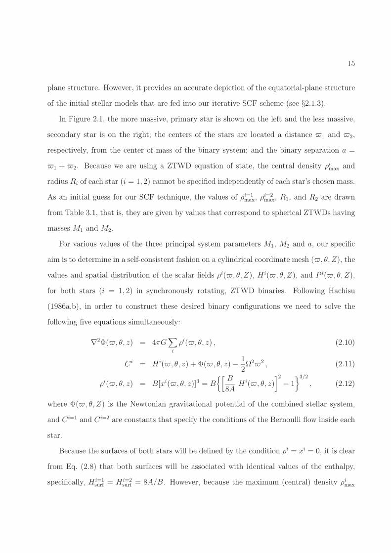
15

plane structure. However, it provides an accurate depiction of the equatorial-plane structure

of the initial stellar models that are fed into our iterative SCF scheme (see §2.1.3).

In Figure 2.1, the more massive, primary star is shown on the left and the less massive,

secondary star is on the right; the centers of the stars are located a distance 1 and 2,

respectively, from the center of mass of the binary system; and the binary separation a =

1 + 2. Because we are using a ZTWD equation of state, the central density ρimax and

radius Ri of each star (i = 1, 2) cannot be specified independently of each star’s chosen mass.

As an initial guess for our SCF technique, the values of ρi=1max, ρi=2

max, R1, and R2 are drawn

from Table 3.1, that is, they are given by values that correspond to spherical ZTWDs having

masses M1 and M2.

For various values of the three principal system parameters M1, M2 and a, our specific

aim is to determine in a self-consistent fashion on a cylindrical coordinate mesh (, θ, Z), the

values and spatial distribution of the scalar fields ρi(, θ, Z), H i(, θ, Z), and P i(, θ, Z),

for both stars (i = 1, 2) in synchronously rotating, ZTWD binaries. Following Hachisu

(1986a,b), in order to construct these desired binary configurations we need to solve the

following five equations simultaneously:

∇2Φ(, θ, z) = 4πG∑

i

ρi(, θ, z) , (2.10)

Ci = H i(, θ, z) + Φ(, θ, z) −1

2Ω22 , (2.11)

ρi(, θ, z) = B[xi(, θ, z)]3 = B[

B

8AH i(, θ, z)

]2

− 13/2

, (2.12)

where Φ(, θ, Z) is the Newtonian gravitational potential of the combined stellar system,

and Ci=1 and Ci=2 are constants that specify the conditions of the Bernoulli flow inside each

star.

Because the surfaces of both stars will be defined by the condition ρi = xi = 0, it is clear

from Eq. (2.8) that both surfaces will be associated with identical values of the enthalpy,

specifically, H i=1surf = H i=2

surf = 8A/B. However, because the maximum (central) density ρimax

16

in the two stars generally will not be the same (they will be the same only if the mass ratio

q = 1), the enthalpy at the centers of the two stars generally will be different, namely,

H imax =

8A

B

[

(ximax)

2 + 1]1/2

, (2.13)

where,

ximax ≡

(

ρimax

B

)1/3

. (2.14)

Following Hachisu (1986a), we choose to work in terms of the following dimensionless

variables,

ˆ ≡

∗

, z ≡z

∗

, (2.15)

ρi ≡ρi

ρ∗

, (2.16)

P i ≡P i

G2∗ρ

2∗

, (2.17)

H i ≡H i

G2∗ρ∗

, (2.18)

φ ≡Φ

G2∗ρ∗

, (2.19)

Ω ≡Ω

(Gρ∗)1/2, (2.20)

where ∗ = α is the distance from the orbital axis to the outer edge of the secondary star

(point Oα in Figure 2.1) as measured in the equatorial plane of the system, and ρ∗ ≡ ρi=2max is

the maximum density of the secondary star. In terms of these dimensionless variables, the

key equations (2.10), (2.11), and (2.12) become,

∇2φ( ˆ , θ, z) = 4π∑

i

ρi( ˆ , θ, z) , (2.21)

Ci = H i( ˆ , θ, z) + φ( ˆ , θ, z) −1

2Ω2 ˆ 2 , (2.22)

ρi( ˆ , θ, z) =[

xi( ˆ , θ, z)

x∗

]3

, (2.23)

17

where, x∗ ≡ (ρ∗/B)1/3. In order to relate xi in Eq. (2.23) back to H i in Eq. (2.22) we note

that, via Eqs. (2.8) and (2.13),

(

H i

H imax

)2

=(

H i

H imax

)2

=(xi)2 + 1

(ximax)

2 + 1. (2.24)

Hence, taking into consideration the natural limits on xi inside both stars (namely, ximax ≥

xi > 0), we deduce,

xi =(

H i

H imax

)2

[(ximax)

2 + 1] − 11/2

forH i

H imax

> [(ximax)

2 + 1]−1/2 (2.25)

= 0 forH i

H imax

< [(ximax)

2 + 1]−1/2 .

2.1.3 Solution Strategy

Our solution strategy is as follows. A “guess” is made for the density distribution ρi( ˆ , θ, z)

inside both stars. The Poisson Eq. (2.21) is then solved in order to obtain a quantitative

description of the gravitational potential φ( ˆ , θ, z) throughout the computational domain

that is consistent with the trial density distribution. With this knowledge of φ( ˆ , θ, z),

Eq. (2.22) is used to determine the two constants Ci=2 and Ω by specifying a value for the

entropy at two “boundary” points — points at two different locations on the surface of the

secondary star. By specifying a value for the enthalpy at an additional “boundary” point

at the center of the primary star, Eq. (2.22) also can be used to determine Ci=1. From the

calculated values of Ci=2 and Ω, Eq. (2.22) (with i set to “2”) is used to determine H i=2

throughout the secondary star; and from the calculated values of Ci=1 and Ω, the same

equation (with i = 1) is used to determine H i=1 throughout the primary star. Finally, from

a knowledge of H i, Eq. (2.25) is used to determine xi, then Eq. (2.23) is used to determine

ρi throughout the interiors of both stars. This revised density profile for both stars is used

as an improved “guess” for our iteration scheme and all of the outlined steps are repeated

until a converged solution is reached.

18

Although our ultimate desire is to construct a model of a binary system that has a

specified total mass and mass ratio, the values of the individual stellar masses are not

constrained to remain constant throughout the cycles of our iteration scheme. Instead, we

fix the values of xi=1max and xi=2

max throughout the iteration until a converged solution has

been reached. This proves to be an effective approach because, as pointed out by Hachisu

(1986a,b), this type of SCF scheme converges more rapidly if the maximum density rather

than the mass is held fixed. Also, for the ZTWD equation of state, we know that xmax is

correlated with the stellar mass (see Table 3.1 and the upper left panel of Figure 1.1). In

practice, if the mass of either star in a converged model does not match some desired value,

we simply rerun the iteration scheme using an appropriately adjusted value of xmax. In what

follows, each of the steps in our SCF iteration scheme is described in more detail.

Initial Guess for ρi and Determination of φ

As with most successful iterative solution schemes, our SCF technique can converge relatively

quickly to a desired solution if the initial guess for the relevant scalar fields is a good one. As

mentioned earlier, our initial guess is two spherical white dwarfs having masses M1 and M2

in a circular orbit with a separation a (as depicted in Figure 2.1) and an orbital frequency,

Ω = (GMtot/a3)1/2, that is, Ω = [Mtot/(a

3ρ∗)]1/2. For all but perhaps the smallest allowed

separations, this should provide an excellent starting condition. For the specified pair of

masses, Table 3.1 provides the appropriate values of various physical parameters, such as Ri,

ρimax, and xi

max, for both stars. In addition, the spherical models from which the data in Table

3.1 were derived provide an initial guess for the density structure ρi(, θ, z) throughout the

interiors of both stars. In order to transform these density arrays into the dimensionless

densities ρi defined by Eq. (2.16), the profiles for both stars are normalized to ρ∗ ≡ ρi=2max

before they are introduced into the cylindrical coordinate grid.

To be consistent with the dimensionless length scale defined by Eq. (2.15), the two

19

spherical stars are initially placed on the computational grid in such a way that the center

of mass of the system falls at the origin of the coordinate system and the outer edge of the

secondary star (point Oα in Figure 2.1) is at ˆ = 1. The centers of the stars are therefore

located, respectively, at

ˆ 1 ≡1

α

=q

1 + ℓ(1 + q), (2.26)

ˆ 2 ≡2

α

=1

1 + ℓ(1 + q), (2.27)

where the dimensionless ratio ℓ ≡ R2/a is known once M2 and a have been chosen. These

two expressions make sense because α = (2+aℓ) = [2+(2+1)ℓ] and, for a point-mass

binary whose center of mass is at the origin of the grid, 1 = q2.

With ρi defined everywhere on the grid, φ( ˆ , θ, z) is calculated via Eq. (2.21). In this

work the boundary values for φ are calculated using the compact cylindrical Green’s function

expansion described in Cohl & Tohline (1999), and the values of the potential throughout the

interior volume of the computational grid are calculated using the Krylov subspace methods

provided by the PETSc software library (Balay et al (2004)). See further discussions in

§2.2.

Secondary Star

During the iteration cycles we calculate new or updated values of the two constants Ci=2

and Ω by enforcing boundary conditions at the inner and outer edges of the secondary star

– the points marked Oβ and Oα in Figure 2.1 – and the coordinate locations of these two

points are held fixed. Pinning down the location of points Oα and Oβ prevents the geometric

structure of the binary from varying dramatically from the initial configuration during the

iterations. Because these two points lie on the surface of the secondary star and, hence,

Hα = Hβ = H i=2surf , an evaluation of Eq. (2.22) at these points gives,

Ω2 =2[φα − φβ]

[1 − ˆ 2β]

, (2.28)

20

where the subscripts α and β imply that the variables have been evaluated at points Oα and

Oβ, respectively.

Knowledge of Ω2 permits us to calculate values of the function,

F ≡ −φ +1

2Ω2 ˆ 2 , (2.29)

across the entire computational domain. From Eq. (2.22) we realize that this function also

may be written as,

F = (H i − Ci) , (2.30)

that is, it differs from the enthalpy by only a constant. Therefore, in the region occupied

by the secondary star, H i=2, ρi=2, and xi=2 should all assume their maximum values at the

same coordinate location where the function F reaches a local maximum, that is, at the

location of F i=2max. This, then, becomes the updated position for point O2 (see Figure 2.1).

Using Eq. (2.30) in conjunction with Eq. (2.24) evaluated at point Oα (where x = xi=2α = 0)

allows us to determine the value of the constant Ci=2. Specifically,

Hα

H i=2max

=Fα + Ci=2

F i=2max + Ci=2

=[

1

(xi=2max)

2 + 1

]1/2

. (2.31)

Hence,

Ci=2 =

F i=2max − [1 + (xi=2

max)2]1/2Fα

[1 + (xi=2max)

2]1/2 − 1

. (2.32)

With the value of the constant Ci=2 in hand, we can determine the value of the enthalpy

everywhere inside the secondary star via the expression,

H i=2 = Ci=2 + F i=2 , (2.33)

and, in particular,

H i=2max = Ci=2 + F i=2

max . (2.34)

21

Finally, then, from equations (2.23) and (2.25) we obtain an updated “guess” for the nor-

malized density distribution inside the secondary star, that is,

ρi=2 =1

x3∗

(

H i=2

H i=2max

)2

[(xi=2max)

2 + 1] − 13/2

. (2.35)

Primary Star

Using Eq. (2.13), we can determine the value of the normalized enthalpy at the center of

the primary star from the values of ximax selected for both stars and the value of H i=2

max just

derived for the secondary star. Specifically,

H i=1max = H i=2

max

[

(xi=1max)

2 + 1

(xi=2max)

2 + 1

]1/2

. (2.36)

In the vicinity of the original center of the primary star, that is, in the vicinity of point O1 as

illustrated in Figure 2.1, the function F should exhibit a local maximum. We associate the

location of this local maximum with the updated position of point O1 and we set F i=1max equal

to the value of the function at this local maximum. We therefore deduce from Eq. (2.30)

that,

Ci=1 = H i=1max − F i=1

max. (2.37)

With this constant in hand, the normalized enthalpy throughout the primary star can be

determined via the expression,

H i=1 = Ci=1 + F i=1 , (2.38)

and, by analogy with equation (2.35), we obtain an updated “guess” for the normalized

density distribution inside the primary star via the expression,

ρi=1 =1

x3∗

(

H i=1

H i=1max

)2

[(xi=1max)

2 + 1] − 13/2

. (2.39)

22

Global Properties and Convergence

Our iterative scheme is judged to be operating well if various calculated model parameters

— such as the dimensionless stellar masses M i and Bernoulli constants Ci — converge

toward well-defined values. We also have found it useful to track the convergence of various

global energy parameters. Specifically, at the end of each iteration cycle we calculate the

dimensionless rotational kinetic energy K, gravitational potential energy W , total internal

energy U (see, for example, Eq. (75’) in Chapter XI of Chandrasekhar (1967)), and globally

averaged pressure Π of the model, defined as follows:

K ≡∫ 1

2Ω2 ˆ 2ρdV , (2.40)

W ≡∫ 1

2φρdV , (2.41)

U ≡∫[(

H −8A

B

)

ρ − P]

dV , (2.42)

Π ≡∫

P dV . (2.43)

where dV = ˆ d ˆ dθdz is the dimensionless differential volume element on our cylindrical

grid. Then the system’s dimensionless total energy is given by the sum,

Etot ≡Etot

Gρ2∗

5∗

= K + W + U , (2.44)

and, if the model has converged to a proper equilibrium state, according to the virial theorem

we should expect,

2K + W + 3Π = 0 . (2.45)

In general, at each iteration step the condition of virial equilibrium, Eq. (2.45), will not be

satisfied, but if our iteration scheme is well behaved, convergence toward the virial condition

should be achieved. With this in mind, we have found that the virial error,

V E ≡

∣

∣

∣

∣

2K + W + 3Π

W

∣

∣

∣

∣

, (2.46)

23

Table 2.1. Convergence of SCF Method: Binary Model B3

N Nθ Nz δ VE

64 128 33 1.0 × 10−2 4.5 × 10−3

1.0 × 10−3 2.6 × 10−3

1.4 × 10−4 2.2 × 10−3

128 256 65 1.0 × 10−2 4.0 × 10−3

1.0 × 10−3 9.1 × 10−4

1.0 × 10−4 5.7 × 10−4

3.5 × 10−5 5.4 × 10−4

provides a meaningful measure of the quality of each model.

We declare that satisfactory convergence to a given model has been achieved when the

absolute value of the fractional change between iterations has dropped below a specified

convergence criterion, δ ∼ 10−4, for all of the following quantities: Ci, M i, Ω, K, W , Π, and

the physical value of α.

In addition, the converged model is judged to be a good equilibrium state if the virial

error, VE, is sufficiently small. Table 2.1 illustrates how we were able to achieve a lower virial

error and, hence, a more accurate representation of an equilibrium configuration, by improv-

ing the grid resolution and/or by specifying a tighter convergence criterion. Specifically, the

table shows that as we were constructing binary model B3 (see discussion associated with

Table 3.5, below) we were able to push the VE down from a value ∼ 5 × 10−3 to a value

∼ 5×10−4 by increasing the grid resolution from (64,128,33) to (128,256,65) zones in ( ˆ ,θ,z)

and by pushing δ from 10−2 to 3.5 × 10−5.

After the SCF code has converged to the desired equilibrium model, the various dimen-

sionless variables are converted back to proper physical units following, for example, the

scalings presented in expressions (2.15) through (2.20). We note in particular that the value

of the scale length ∗ = α is obtained by evaluating Eq. (2.13) for i = 2 in combination

24

with Eq. (2.18), which gives,

∗ =[

8A/B

Gρ∗

]1/2

(H i=2max)

−1/2[

(xi=2max)

2 + 1]1/4

. (2.47)

In addition to the physical variables already identified, for each converged model we have

found it useful to evaluate the system’s total angular momentum,

Jtot ≡∫

2ΩρdV , (2.48)

as well as the spin angular momentum of each component star, J ispin, and each star’s Roche-

lobe filling factor, f iRL. As with the determination of quantities such as M i and Ri, these

latter two quantities are obtained by performing volume integrals over appropriate sub-

domains of the computational grid, determined as follows. Let the origin of a Cartesian

grid coincide with the center of mass of the binary system and align the x-axis of that grid

with the line that connects the centers of the two stars as illustrated in Figure 2.1. Between

points O1 and O2 along this axis, the effective potential,

Φeff(x) ≡ Φ(x) −1

2Ω2x2 , (2.49)

will exhibit a maximum at position xL1 associated with the inner “L1” Lagrange point. We

define sub-domain Di=2∗ as the volume of the grid for which x ≡ cos θ ≥ xL1 and ρ > 0,

that is, the region occupied by the secondary star; and we define sub-domain Di=1∗ as the

volume of the grid for which x < xL1 and ρ > 0, that is, the region occupied by the primary

star. Then the mass of each star is determined by the integral,

M i =∫

Di∗

ρidV , (2.50)

the volume occupied by each star is,

V i∗ =

∫

Di∗

dV , (2.51)

25

and the spin angular momentum of each star is given by the expression,

J ispin ≡

∫

Di∗

[2 sin2 θ + ( cos θ − i)2] ΩρidV . (2.52)

Having determined the volumes V i occupied by both rotationally flattened and tidally dis-

torted stars, we define the mean radius of each star as,

Ri =(

3V i∗

4π

)1/3

. (2.53)

We furthermore define sub-domain Di=2RL as the volume of the grid for which x ≥ xL1

and Φeff ≤ Φeff(xL1), and sub-domain Di=1RL as the volume of the grid for which x < xL1 and

Φeff ≤ Φeff(xL1). Then the Roche-lobe volume surrounding each star is,

V iRL =

∫

DiRL

dV , (2.54)

and each star’s Roche-lobe filling factor is obtained from the ratio,

f iRL =

V i∗

V iRL

. (2.55)

2.2 Numerical Solutions for the Gravitational Poten-

tial

The self-gravity of the binary system is one of the most dominate phenomena driving the

evolution of the binary. In order to obtain accurate numerical results in a CFD simulation,

the gravitational potential must be reevaluated at every step in the time integration. The

gravitational potential, Φ, is defined as

Φ(~r) = −∫ ∞

0

Gρ(~r′)d3r′

|~r − ~r′|, (2.56)

where ρ is the mass density, and ~r′ is position vector that is integrated over all space. The

gravitational potential is more commonly calculated by solving the Poisson equation,

∇2Φ = 4πGρ. (2.57)

26

The solution to this elliptic equation requires that all cells in the grid have knowledge of

the value of ρ and Φ at all other cells. In contrast, the hyberbolic equations used to update

the fluid quantities require only knowledge of their neighboring cells. This need to know

the value of the potential everywhere requires extra design consideration when developing a

solver that is going to be implemented in parallel because each CPU in the cluster will only

have local access to the small subset of data on which it is operating. A communication

between the processors allows the nodes on the cluster to share this information with one

another, but inter-processor communication must be kept to a minimum because it is slow

compared to calculations.

In the existing version of our group’s hydrocode (see Chapter 4) and SCF code, an efficient

solver has been developed for the gravitational potential. However, this solver is limited to

coordinate systems in which there is a periodic coordinate because it requires a Fourier

transform. Until the present time all simulations done within the group have been done in

cylindrical coordinate systems, but a more flexible solver is desired so that simulations are

no longer limited to certain coordinate systems. Additionally, the Fourier transform method

is not extensible to adaptive meshes. A variety of numerical packages have been developed

by other groups to solve elliptic equations in parallel environments. For this work, we have

chosen to use elliptic solvers within The Portable Extensible Toolkit for Scientific Computing

(PETSc) and to link these solvers with our hydrodynamics code to solve for the gravitational

potential (Balay et al. 2004).

2.2.1 Numerical Discretization

The Poisson equation in cylindrical coordinates is given by

∂2Φ

∂2+

1

∂Φ

∂+

1

2

∂2Φ

∂θ2+

∂2Φ

∂z2= 4πGρ, (2.58)

where is the radial coordinate, θ is the azimuthal coordinate, and z is the vertical coordi-

nate.

27

Using a second order finite difference scheme for each derivative we obtain the following

formulation:

Φi+1 − 2Φ + Φi−1

(∆)2 +Φi+1 − Φi−1

2∆+

Φj+1 − 2Φ + Φj−1

2 (∆θ)2 +Φk+1 − 2Φ + Φk−1

(∆z)2 = 4πGρ. (2.59)

Collecting the coefficients on Φ,

(

−2

(∆)2 −2

2 (∆θ)2 −2

(∆z)2

)

Φ +

(

1

(∆)2 +1

2∆

)

Φi+1

+

(

1

(∆)2 −1

2∆

)

Φi−1 +1

2 (∆θ)2 Φj+1 +1

2 (∆θ)2 Φj−1

+1

(∆z)2 Φk+1 +1

(∆z)2 Φk−1 = 4πGρ. (2.60)

These coefficients can then be put into a two-dimensional, N ×N sparse matrix A, where N

is the product of the number of radial, azimuthal and vertical divisions. Each row in A has

a maximum of seven non-zero elements. The gravitational potential and density are stored

in 1D arrays and the Poisson equation can be written as,

AΦ = 4πGρ. (2.61)

2.2.2 Test Problems

The solver was tested using two different cases with known analytic solutions: a uniform

density sphere, also known as an n=0 polytrope, and a spherical n=1 polytrope. Polytropes

are stellar structures that have been constructed using the so-called polytropic equation of

state, Eq. (4.9). In the first case, the analytic form of the potential and density are

ρ(rsp) = ρc rsp ≤ Rsp (2.62)

ρ(rsp) = 0 rsp > Rsp (2.63)

Φ(rsp) = −2πGρc

(

R2sp −

r2sp

3

)

rsp ≤ Rsp (2.64)

Φ(rsp) = −4

3πGρc

R3sp

rsp

rsp > Rsp, (2.65)

28

where rsp is the distance from the center of the spherical object and Rsp is the total radius of

the object. The density distribution and potential for a spherical n=1 polytrope are defined

as

ρ(rsp) =ρcRsp sin(πrsp

Rsp)

πrsp

rsp ≤ Rsp (2.66)

ρ(rsp) = 0 rsp > Rsp (2.67)

Φ(rsp) =−4GR2

spρc

π

[

Rsp

rspπsin

(

πrsp

Rsp

)

+ 1

]

rsp ≤ Rsp (2.68)

Φ(r) =−GM

rsp

rsp > Rsp, (2.69)

where M = 4R3spρc/π is the total mass of the spherical object.

The numeric and analytic solutions are compared below for n=0 and n=1 polytropes.

Example configurations are shown in Figure 2.2. The analytic solution used in these com-

parisons was calculated by different methods in the interior and exterior of the star. In the

interior the mass was calculated by solving the exact analytic solutions in the preceding

sections. However, in the exterior region the potential was calculated for a point mass at

the center of the sphere. Instead of using the analytically integrated mass, the mass of the

individual cells was summed to obtain the total mass. This mass was chosen because it

more closely resembles the mass that will be used by the numeric solver for the Poisson

equation. The errors shown in Table 2.2 are percent differences between the numeric and

analytic solutions.

29

Figure 2.2 An n = 0 spherical polytrope. The left plots are the density distributions and theright plots are the error between the numerical and analytic solutions. In the top diagramsthe sphere is centered on the cylindrical axis. On the bottom the center of the sphere hasbeen displaced by 0.5 on the y axis. Blue represents regions of maximum density (left) anderror (right) and dark red represents minimum values. These correspond to the values givenin Table 2.2 for 1283 resolution.

30

Table 2.2. Error of Poisson solver for spherical polytropes

n z θ y displacement Min Error Max Error Avg Error

0 64 64 64 0 1.10 × 10−4 1.41 2.85 × 10−1

1 64 64 64 0 2.40 × 10−3 4.98 × 10−1 2.71 × 10−1

0 64 64 64 0.5 0.00 8.87 × 10−1 7.35 × 10−2

1 64 64 64 0.5 0.00 4.10 × 10−1 8.46 × 10−2

0 128 128 128 0 1.24 × 10−4 4.10 × 10−1 8.46 × 10−2

1 128 128 128 0 1.11 × 10−4 1.69 × 10−1 5.52 × 10−2

0 128 128 128 0.5 6.05 × 10−5 7.02 × 10−1 9.61 × 10−2

1 128 128 128 0.5 0.00 1.52 6.05 × 10−2

3. Steady State Binary Sequences1

As mentioned earlier, we initially used a simplified version of our SCF code to construct

a large number of single, nonrotating white dwarfs in order to compare our solutions with

previous results (see Figure 3.1) and to provide initial guesses for the density distributions

inside both stars in each binary system. Table 3.1 details the properties of single, nonro-

tating white dwarfs that have central densities ranging from 104.5 g cm−3 to 1010 g cm−3 as

determined from our model calculations; the 23 selected models are equally spaced in units

of log ρmax.

These spherical models were constructed on a uniform cylindrical mesh with resolution

(128, 128, 128) in ( ˆ , θ, z) using a convergence criterion δ = 10−4. For each converged model,

the first six columns of Table 3.1 list, respectively, the star’s mass M in solar masses, radius R

in units of 108 cm, central density ρmax in g cm−3, corresponding value of xmax = (ρmax/B)1/3,

moment of inertia,

I =∫

2ρdV , (3.1)

in units of 1050 g cm2, and the radius of gyration, k ≡ I/(MR2). As shown in the last column

of Table 3.1, a typical virial error for these converged models was 10−4 − 10−5. The values

tabulated for the radius of gyration vary smoothly from k = 0.2036 for M = 0.0844M⊙

to k = 0.1013 for M = 1.4081M⊙. (See also the upper right panel of Figure 1.1.) This

is consistent with our understanding that low-mass white dwarfs have structures similar to

n = 3/2 polytropes for which k = 0.205 (Rucinski, 1988), while high-mass white dwarfs

display structures similar to n = 3 polytropes for which k = 0.0758 (Rucinski, 1988). Our

values of k over this range of stellar masses are also consistent with the analytic function for

k(M) that Marsh et al. (2004) fit through similar spherical model data. Knowledge of the

1§2.1 and Chapter 3 reproduced by permission of the AAS (Even & Tohline (2009))

31

32

Table 3.1. Sequence of single, nonrotating ZTWDs.

M R ρmax xmax I k VE(M⊙) (108 cm) (g cm−3) (1050 g cm2)

0.0844 19.7673 3.1623 × 104 0.2526 1.3317 0.2036 1.4 × 10−5

0.1113 17.9368 5.6234 × 104 0.3060 1.4422 0.2031 6.1 × 10−5

0.1460 16.2672 1.0000 × 105 0.3708 1.5508 0.2024 1.4 × 10−5

0.1903 14.7421 1.7783 × 105 0.4492 1.6517 0.2015 5.8 × 10−5

0.2457 13.3464 3.1623 × 105 0.5442 1.7360 0.2001 1.4 × 10−5

0.3134 12.0666 5.6234 × 105 0.6593 1.7936 0.1983 5.8 × 10−5

0.3938 10.8906 1.0000 × 106 0.7988 1.8133 0.1958 5.9 × 10−5

0.4859 9.8078 1.7783 × 106 0.9678 1.7852 0.1926 1.6 × 10−5

0.5873 8.8097 3.1623 × 106 1.1725 1.7051 0.1887 6.1 × 10−5

0.6942 7.8896 5.6234 × 106 1.4205 1.5754 0.1839 5.8 × 10−5

0.8018 7.0419 1.0000 × 107 1.7209 1.4058 0.1783 7.6 × 10−5

0.9058 6.2628 1.7783 × 107 2.0850 1.2122 0.1721 6.6 × 10−5

1.0022 5.5487 3.1623 × 107 2.5260 1.0111 0.1653 5.1 × 10−5

1.0882 4.8961 5.6234 × 107 3.0603 0.8176 0.1581 6.3 × 10−5

1.1624 4.3023 1.0000 × 108 3.7076 0.6429 0.1507 6.3 × 10−5

1.2246 3.7643 1.7783 × 108 4.4919 0.4929 0.1433 7.0 × 10−5

1.2753 3.2793 3.1623 × 108 5.4421 0.3698 0.1360 7.4 × 10−5

1.3155 2.8443 5.6234 × 108 6.5932 0.2723 0.1290 9.0 × 10−5

1.3469 2.4560 1.0000 × 109 7.9879 0.1972 0.1225 1.1 × 10−4

1.3708 2.1116 1.7783 × 109 9.6775 0.1410 0.1164 1.2 × 10−4

1.3887 1.8078 3.1623 × 109 11.7246 0.0997 0.1108 1.3 × 10−4

1.4020 1.5414 5.6234 × 109 14.2047 0.0699 0.1058 1.4 × 10−4

1.4116 1.3092 1.0000 × 1010 17.2094 0.0486 0.1013 1.4 × 10−4

33

Figure 3.1 The mass-radius relationship is shown for spherical stars with our adopted ZTWDequation of state. Diamonds represent results derived using our three-dimensional SCFscheme applied to nonrotating, isolated configurations (see Table 3.1); asterisks show previ-ously published results for the same equation of state taken from Hachisu (1986a); the solidcurve shows the analytic mass-radius relation, Eq. (A.14), derived by Nauenberg (1972).

radius of gyration of these spherical ZTWD models has assisted us in analyzing the tidally

distorted structures that arise in our models of synchronously rotating white dwarfs in close

binary systems (see further discussion, below).

Using this same 3D, cylindrical coordinate grid we constructed nonrotating models with

central densities above 1010 g cm−3, that is, with masses above 1.4M⊙. We have not included

these higher mass models in Table 3.1 or Figure 3.1, however, because they did not converge

to satisfactorily accurate structures. In particular, as the mass was steadily increased above

34

1.4M⊙, the models converged to structures with steadily increasing (rather than decreasing)

values of k. By contrast, as shown in Figure 1.1 models constructed using a one-dimensional

spherical code with much higher spatial resolution displayed values of k that decreased

steadily to a value of 0.0755 at masses approaching Mch. If desired, the three-dimensional

computational grid resolution could be increased to produce more accurate models of the

white dwarf structure near the Chandrasekhar mass limit.

3.1 Inspiral White Dwarf Binary Sequences

The slow inspiral evolution of a DWD binary can be mimicked by constructing a sequence of

detached binaries having fixed Mtot and fixed q but varying separation, down to the separa-

tion, acrit, at which the less massive star first makes contact with its Roche lobe. In an effort

to illustrate the capabilities of our SCF code, we have constructed three binary sequences

having the same total mass — namely, Mtot = 1.5M⊙ — but three separate mass ratios.

Specifically, sequence ‘A’ has q = 1, sequence ‘B’ has q = 2/3, and sequence ‘C’ has q = 1/2.

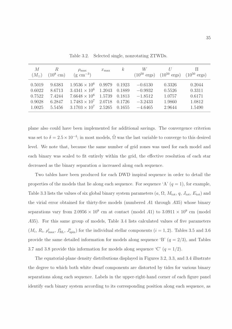
As detailed in Table 3.2, spherical models were constructed with the desired primary and sec-

ondary masses for these three sequences — specifically, M = 0.5M⊙, 0.6M⊙, 0.75M⊙, 0.9M⊙

and 1.0M⊙ — to provide good “guesses” for the initial binary star density distributions to

start each SCF iteration. In addition to listing the values of M , R, ρmax, xmax, and k for

each of these converged spherical models, as was done for a wider range of spherical models

in Table 3.1, Table 3.2 also lists values for the global energies W , U , and Π in units of 1050

ergs.

Along each sequence, all the binary models were constructed using a uniform cylindrical

grid with (128,256,65) zones in ( ˆ , θ, z); by implementing reflection symmetry through the

equatorial plane, only half as many zones were needed in the vertical direction as in the radial

direction to achieve the same resolution in both. No additional symmetries were assumed in

constructing the sequence, although, for the models shown here, symmetry through the x-z

35

Table 3.2. Selected single, nonrotating ZTWDs.

M R ρmax xmax k W U Π(M⊙) (108 cm) (g cm−3) (1050 ergs) (1050 ergs) (1050 ergs)

0.5019 9.6383 1.9536 × 106 0.9979 0.1923 −0.6130 0.3326 0.20440.6022 8.6713 3.4341 × 106 1.2043 0.1889 −0.9932 0.5526 0.33110.7522 7.4244 7.6648 × 106 1.5739 0.1813 −1.8512 1.0757 0.61710.9028 6.2847 1.7483 × 107 2.0718 0.1726 −3.2433 1.9860 1.08121.0025 5.5456 3.1703 × 107 2.5265 0.1655 −4.6465 2.9644 1.5490

plane also could have been implemented for additional savings. The convergence criterion

was set to δ = 2.5×10−4; in most models, Ω was the last variable to converge to this desired

level. We note that, because the same number of grid zones was used for each model and

each binary was scaled to fit entirely within the grid, the effective resolution of each star

decreased as the binary separation a increased along each sequence.

Two tables have been produced for each DWD inspiral sequence in order to detail the

properties of the models that lie along each sequence. For sequence ‘A’ (q = 1), for example,

Table 3.3 lists the values of six global binary system parameters (a, Ω, Mtot, q, Jtot, Etot) and

the virial error obtained for thirty-five models (numbered A1 through A35) whose binary

separations vary from 2.0956 × 109 cm at contact (model A1) to 3.0911 × 109 cm (model

A35). For this same group of models, Table 3.4 lists calculated values of five parameters

(Mi, Ri, ρimax, f i

RL, J ispin) for the individual stellar components (i = 1, 2). Tables 3.5 and 3.6

provide the same detailed information for models along sequence ‘B’ (q = 2/3), and Tables

3.7 and 3.8 provide this information for models along sequence ‘C’ (q = 1/2).

The equatorial-plane density distributions displayed in Figures 3.2, 3.3, and 3.4 illustrate

the degree to which both white dwarf components are distorted by tides for various binary

separations along each sequence. Labels in the upper-right-hand corner of each figure panel

identify each binary system according to its corresponding position along each sequence, as

36

Table 3.3. DWD Inspiral Sequence ‘A’: Mtot = 1.5M⊙; q = 1

Model a Ω Mtot q Jtot Etot VE(109 cm) (10−2 s−1) (M⊙) (1050 cgs) (1050 erg)

A1 2.0956 14.8480 1.5045 1.0000 5.3879 −1.8624 2.7 × 10−4

A2 2.0970 14.8317 1.5043 1.0000 5.3881 −1.8618 2.8 × 10−4

A3 2.1042 14.7493 1.5036 1.0000 5.3882 −1.8589 2.8 × 10−4

A4 2.1099 14.6847 1.5030 1.0000 5.3886 −1.8567 2.9 × 10−4

A5 2.1162 14.6156 1.5031 1.0000 5.3915 −1.8566 2.7 × 10−4

A6 2.1239 14.5339 1.5031 1.0000 5.3954 −1.8560 2.7 × 10−4

A7 2.1428 14.3360 1.5032 1.0000 5.4059 −1.8549 2.8 × 10−4

A8 2.1544 14.2154 1.5030 1.0000 5.4112 −1.8532 2.9 × 10−4

A9 2.1671 14.0863 1.5029 1.0000 5.4180 −1.8519 2.9 × 10−4

A10 2.1809 13.9475 1.5028 1.0000 5.4254 −1.8508 2.6 × 10−4

A11 2.1960 13.7990 1.5027 1.0000 5.4337 −1.8490 2.7 × 10−4

A12 2.2292 13.4849 1.5030 1.0000 5.4554 −1.8471 2.6 × 10−4

A13 2.2479 13.3121 1.5027 1.0000 5.4665 −1.8448 2.7 × 10−4

A14 2.2669 13.1429 1.5032 1.0000 5.4814 −1.8447 2.7 × 10−4

A15 2.2880 12.9570 1.5030 1.0000 5.4944 −1.8421 2.7 × 10−4

A16 2.3103 12.7655 1.5027 1.0000 5.5082 −1.8392 2.8 × 10−4

A17 2.3572 12.3804 1.5029 1.0000 5.5423 −1.8359 2.8 × 10−4

A18 2.3828 12.1772 1.5027 1.0000 5.5597 −1.8329 2.8 × 10−4

A19 2.4092 11.9748 1.5028 1.0000 5.5792 −1.8307 2.8 × 10−4

A20 2.4362 11.7751 1.5032 1.0000 5.6013 −1.8298 2.8 × 10−4

A21 2.4652 11.5645 1.5030 1.0000 5.6221 −1.8265 2.9 × 10−4

A22 2.5261 11.1442 1.5030 1.0000 5.6684 −1.8215 2.8 × 10−4

A23 2.5584 10.9314 1.5030 1.0000 5.6928 −1.8185 2.9 × 10−4

A24 2.5920 10.7176 1.5028 1.0000 5.7185 −1.8151 3.1 × 10−4

A25 2.6264 10.5057 1.5029 1.0000 5.7457 −1.8127 3.0 × 10−4

A26 2.6624 10.2904 1.5028 1.0000 5.7729 −1.8093 3.0 × 10−4

A27 2.6991 10.0786 1.5029 1.0000 5.8016 −1.8068 2.9 × 10−4

A28 2.7376 9.8598 1.5028 1.0000 5.8286 −1.8039 1.5 × 10−4

A29 2.8175 9.4479 1.5031 1.0000 5.8981 −1.7984 3.2 × 10−4

A30 2.8597 9.2377 1.5031 1.0000 5.9315 −1.7951 3.2 × 10−4

A31 2.8784 9.1459 1.5027 1.0000 5.9440 −1.7925 3.2 × 10−4

A32 2.9478 8.8242 1.5032 1.0000 6.0024 −1.7892 3.3 × 10−4

A33 2.9940 8.6120 1.5031 1.0000 6.0336 −1.7860 1.9 × 10−4

A34 3.0420 8.4102 1.5031 1.0000 6.0738 −1.7827 2.1 × 10−4

A35 3.0911 8.2099 1.5032 1.0000 6.1135 −1.7797 2.2 × 10−4

37

Table 3.4. Individual Stellar Components along DWD Inspiral Sequence ‘A’

Model M1 R1 ρi=1max f i=1

RL J i=1spin M2 R2 ρi=2

max f i=2RL J i=2

spin

(M⊙) (109 cm) (109 cgs) (1050 cgs) (M⊙) (109 cm) (109 cgs) (1050 cgs)

A1 0.7522 0.7841 6.745 1.0000 0.2562 0.7522 0.7841 6.745 1.0000 0.2562A2 0.7522 0.7840 6.745 0.9969 0.2559 0.7522 0.7840 6.745 0.9969 0.2559A3 0.7518 0.7835 6.745 0.9838 0.2540 0.7518 0.7835 6.745 0.9838 0.2540A4 0.7515 0.7831 6.745 0.9736 0.2526 0.7515 0.7831 6.745 0.9736 0.2526A5 0.7516 0.7825 6.758 0.9614 0.2509 0.7516 0.7825 6.758 0.9615 0.2509A6 0.7516 0.7817 6.771 0.9471 0.2489 0.7516 0.7817 6.771 0.9471 0.2489A7 0.7516 0.7798 6.805 0.9134 0.2441 0.7516 0.7798 6.805 0.9134 0.2441A8 0.7515 0.7790 6.820 0.8942 0.2414 0.7515 0.7790 6.820 0.8942 0.2414A9 0.7514 0.7780 6.837 0.8739 0.2384 0.7514 0.7780 6.837 0.8739 0.2384

A10 0.7514 0.7769 6.855 0.8523 0.2353 0.7514 0.7769 6.855 0.8523 0.2353A11 0.7513 0.7759 6.876 0.8303 0.2320 0.7513 0.7758 6.876 0.8303 0.2320A12 0.7515 0.7735 6.924 0.7838 0.2250 0.7515 0.7735 6.924 0.7838 0.2250A13 0.7514 0.7724 6.944 0.7602 0.2213 0.7514 0.7724 6.944 0.7602 0.2213A14 0.7516 0.7711 6.977 0.7367 0.2176 0.7516 0.7711 6.977 0.7367 0.2176A15 0.7515 0.7701 6.992 0.7131 0.2138 0.7515 0.7701 6.992 0.7131 0.2138A16 0.7513 0.7692 7.013 0.6903 0.2099 0.7513 0.7692 7.013 0.6903 0.2099

38

Table 3.4—Continued



max f i=2RL J i=2

spin


A17 0.7515 0.7668 7.062 0.6440 0.2020 0.7515 0.7668 7.062 0.6440 0.2020A18 0.7514 0.7658 7.083 0.6215 0.1980 0.7514 0.7658 7.083 0.6215 0.1980A19 0.7514 0.7650 7.103 0.5998 0.1940 0.7514 0.7650 7.103 0.5998 0.1940A20 0.7516 0.7637 7.137 0.5779 0.1901 0.7516 0.7637 7.137 0.5779 0.1901A21 0.7515 0.7629 7.153 0.5568 0.1861 0.7515 0.7629 7.153 0.5567 0.1861A22 0.7515 0.7611 7.198 0.5160 0.1781 0.7515 0.7611 7.198 0.5160 0.1781A23 0.7515 0.7603 7.214 0.4964 0.1742 0.7515 0.7603 7.214 0.4964 0.1742A24 0.7514 0.7596 7.234 0.4774 0.1703 0.7514 0.7596 7.234 0.4774 0.1703A25 0.7515 0.7585 7.251 0.4583 0.1664 0.7515 0.7585 7.251 0.4583 0.1664A26 0.7514 0.7579 7.271 0.4404 0.1625 0.7514 0.7579 7.271 0.4404 0.1625A27 0.7514 0.7571 7.290 0.4231 0.1587 0.7514 0.7571 7.290 0.4231 0.1587A28 0.7514 0.7562 7.309 0.4057 0.1548 0.7514 0.7562 7.309 0.4057 0.1548A29 0.7516 0.7548 7.349 0.3733 0.1476 0.7516 0.7548 7.349 0.3733 0.1476A30 0.7515 0.7541 7.363 0.3575 0.1440 0.7515 0.7541 7.363 0.3576 0.1440A31 0.7513 0.7540 7.363 0.3478 0.1424 0.7513 0.7541 7.363 0.3518 0.1424A32 0.7516 0.7529 7.397 0.3282 0.1369 0.7516 0.7529 7.397 0.3282 0.1369A33 0.7515 0.7522 7.412 0.3142 0.1333 0.7515 0.7522 7.412 0.3142 0.1333A34 0.7516 0.7517 7.425 0.3005 0.1299 0.7516 0.7517 7.425 0.3005 0.1299A35 0.7516 0.7511 7.438 0.2874 0.1265 0.7516 0.7510 7.440 0.2873 0.1265

39

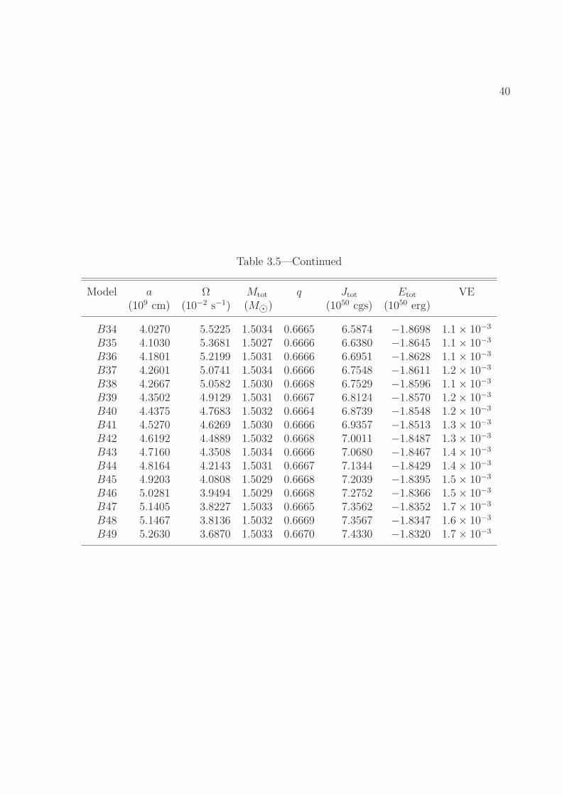
Table 3.5. DWD Inspiral Sequence ‘B’: Mtot = 1.5M⊙; q = 2/3


B1 2.6679 10.2944 1.5042 0.6671 5.5888 −1.9460 6.0 × 10−4

B2 2.6743 10.2576 1.5043 0.6667 5.5931 −1.9460 6.1 × 10−4

B3 2.6819 10.2106 1.5037 0.6667 5.5951 −1.9436 6.0 × 10−4

B4 2.6923 10.1491 1.5033 0.6664 5.6001 −1.9419 6.1 × 10−4

B5 2.7039 10.0831 1.5036 0.6663 5.6090 −1.9420 6.0 × 10−4

B6 2.7177 10.0040 1.5034 0.6665 5.6174 −1.9401 6.1 × 10−4

B7 2.7487 9.8330 1.5035 0.6665 5.6403 −1.9383 6.2 × 10−4

B8 2.7687 9.7249 1.5035 0.6664 5.6542 −1.9372 6.2 × 10−4

B9 2.7902 9.6104 1.5033 0.6665 5.6684 −1.9348 6.3 × 10−4

B10 2.8138 9.4879 1.5033 0.6664 5.6851 −1.9333 6.3 × 10−4

B11 2.8388 9.3609 1.5033 0.6663 5.7034 −1.9318 6.4 × 10−4

B12 2.8654 9.2290 1.5032 0.6665 5.7224 −1.9295 6.4 × 10−4

B13 2.9196 8.9712 1.5034 0.6665 5.7638 −1.9267 6.5 × 10−4

B14 2.9514 8.8246 1.5033 0.6665 5.7864 −1.9241 6.8 × 10−4

B15 2.9850 8.6746 1.5031 0.6665 5.8108 −1.9215 6.8 × 10−4

B16 3.0199 8.5240 1.5034 0.6664 5.8380 −1.9201 6.9 × 10−4

B17 3.0567 8.3680 1.5031 0.6665 5.8638 −1.9170 7.0 × 10−4

B18 3.0949 8.2123 1.5032 0.6665 5.8928 −1.9147 7.0 × 10−4

B19 3.1350 8.0548 1.5034 0.6663 5.9238 −1.9132 7.2 × 10−4

B20 3.1766 7.8955 1.5031 0.6665 5.9543 −1.9097 7.4 × 10−4

B21 3.2199 7.7355 1.5032 0.6666 5.9870 −1.9074 7.5 × 10−4

B22 3.2653 7.5743 1.5034 0.6664 6.0218 −1.9056 7.8 × 10−4

B23 3.3554 7.2699 1.5033 0.6667 6.0905 −1.9002 8.1 × 10−4

B24 3.4062 7.1070 1.5034 0.6666 6.1285 −1.8978 8.1 × 10−4

B25 3.4590 6.9440 1.5034 0.6665 6.1681 −1.8951 8.5 × 10−4

B26 3.5133 6.7821 1.5032 0.6666 6.2078 −1.8917 8.6 × 10−4

B27 3.5700 6.6211 1.5033 0.6665 6.2506 −1.8893 8.8 × 10−4

B28 3.6285 6.4611 1.5034 0.6665 6.2948 −1.8867 9.2 × 10−4

B29 3.6892 6.3010 1.5032 0.6666 6.3387 −1.8832 9.3 × 10−4

B30 3.7520 6.1432 1.5033 0.6666 6.3860 −1.8809 9.6 × 10−4

B31 3.8171 5.9860 1.5034 0.6665 6.4340 −1.8783 9.9 × 10−4

B32 3.8846 5.8298 1.5032 0.6667 6.4828 −1.8747 1.0 × 10−3

B33 3.9544 5.6759 1.5034 0.6666 6.5344 −1.8724 1.0 × 10−3

40



B34 4.0270 5.5225 1.5034 0.6665 6.5874 −1.8698 1.1 × 10−3

B35 4.1030 5.3681 1.5027 0.6666 6.6380 −1.8645 1.1 × 10−3

B36 4.1801 5.2199 1.5031 0.6666 6.6951 −1.8628 1.1 × 10−3

B37 4.2601 5.0741 1.5034 0.6666 6.7548 −1.8611 1.2 × 10−3

B38 4.2667 5.0582 1.5030 0.6668 6.7529 −1.8596 1.1 × 10−3

B39 4.3502 4.9129 1.5031 0.6667 6.8124 −1.8570 1.2 × 10−3

B40 4.4375 4.7683 1.5032 0.6664 6.8739 −1.8548 1.2 × 10−3

B41 4.5270 4.6269 1.5030 0.6666 6.9357 −1.8513 1.3 × 10−3

B42 4.6192 4.4889 1.5032 0.6668 7.0011 −1.8487 1.3 × 10−3

B43 4.7160 4.3508 1.5034 0.6666 7.0680 −1.8467 1.4 × 10−3

B44 4.8164 4.2143 1.5031 0.6667 7.1344 −1.8429 1.4 × 10−3

B45 4.9203 4.0808 1.5029 0.6668 7.2039 −1.8395 1.5 × 10−3

B46 5.0281 3.9494 1.5029 0.6668 7.2752 −1.8366 1.5 × 10−3

B47 5.1405 3.8227 1.5033 0.6665 7.3562 −1.8352 1.7 × 10−3

B48 5.1467 3.8136 1.5032 0.6669 7.3567 −1.8347 1.6 × 10−3

B49 5.2630 3.6870 1.5033 0.6670 7.4330 −1.8320 1.7 × 10−3

41Table 3.6. Individual Stellar Components along DWD Inspiral Sequence ‘B’



max f i=2RL J i=2

spin


B1 0.9023 0.6345 17.049 0.1913 0.1289 0.6019 0.9117 3.076 1.0001 0.2004B2 0.9026 0.6344 17.049 0.1898 0.1283 0.6017 0.9113 3.076 0.9908 0.1995B3 0.9022 0.6345 17.049 0.1881 0.1278 0.6015 0.9108 3.076 0.9805 0.1982B4 0.9022 0.6343 17.049 0.1856 0.1270 0.6012 0.9101 3.076 0.9667 0.1966B5 0.9023 0.6343 17.047 0.1832 0.1261 0.6013 0.9090 3.083 0.9504 0.1948B6 0.9021 0.6343 17.059 0.1803 0.1250 0.6013 0.9078 3.089 0.9314 0.1927B7 0.9022 0.6340 17.082 0.1737 0.1228 0.6013 0.9056 3.108 0.8916 0.1882B8 0.9022 0.6336 17.085 0.1694 0.1213 0.6012 0.9043 3.115 0.8677 0.1854B9 0.9020 0.6336 17.100 0.1654 0.1198 0.6012 0.9029 3.123 0.8430 0.1825

B10 0.9021 0.6334 17.112 0.1610 0.1182 0.6011 0.9017 3.134 0.8181 0.1795B11 0.9022 0.6334 17.121 0.1565 0.1165 0.6011 0.9003 3.144 0.7917 0.1764B12 0.9020 0.6332 17.139 0.1520 0.1148 0.6012 0.8987 3.153 0.7650 0.1732B13 0.9022 0.6329 17.162 0.1432 0.1114 0.6013 0.8963 3.175 0.7172 0.1670B14 0.9021 0.6326 17.177 0.1383 0.1095 0.6012 0.8950 3.184 0.6907 0.1636B15 0.9020 0.6324 17.195 0.1335 0.1076 0.6011 0.8935 3.194 0.6644 0.1602B16 0.9022 0.6323 17.203 0.1288 0.1056 0.6012 0.8925 3.203 0.6403 0.1568B17 0.9020 0.6323 17.222 0.1241 0.1036 0.6011 0.8914 3.213 0.6158 0.1534B18 0.9020 0.6318 17.241 0.1192 0.1016 0.6012 0.8902 3.223 0.5916 0.1500B19 0.9022 0.6316 17.246 0.1145 0.0995 0.6012 0.8887 3.233 0.5675 0.1465B20 0.9019 0.6315 17.268 0.1099 0.0975 0.6012 0.8879 3.242 0.5448 0.1431B21 0.9020 0.6311 17.287 0.1053 0.0955 0.6012 0.8866 3.251 0.5219 0.1397B22 0.9022 0.6311 17.294 0.1009 0.0933 0.6012 0.8856 3.261 0.5003 0.1364B23 0.9020 0.6307 17.340 0.0928 0.0895 0.6013 0.8837 3.280 0.4605 0.1301B24 0.9021 0.6304 17.353 0.0885 0.0874 0.6013 0.8829 3.285 0.4408 0.1268

42Table 3.6—Continued



max f i=2RL J i=2

spin


B25 0.9021 0.6302 17.362 0.0844 0.0853 0.6012 0.8823 3.294 0.4219 0.1235B26 0.9019 0.6303 17.384 0.0806 0.0833 0.6013 0.8814 3.301 0.4029 0.1203B27 0.9021 0.6301 17.398 0.0767 0.0812 0.6012 0.8804 3.309 0.3846 0.1171B28 0.9021 0.6297 17.409 0.0729 0.0792 0.6013 0.8791 3.316 0.3661 0.1140B29 0.9019 0.6298 17.432 0.0694 0.0772 0.6013 0.8790 3.323 0.3500 0.1109B30 0.9021 0.6292 17.445 0.0657 0.0752 0.6013 0.8780 3.330 0.3334 0.1078B31 0.9021 0.6293 17.457 0.0624 0.0732 0.6013 0.8772 3.336 0.3174 0.1048B32 0.9019 0.6288 17.480 0.0591 0.0712 0.6013 0.8768 3.343 0.3024 0.1019B33 0.9020 0.6289 17.495 0.0560 0.0693 0.6013 0.8762 3.349 0.2879 0.0990B34 0.9021 0.6291 17.504 0.0531 0.0674 0.6013 0.8753 3.355 0.2734 0.0961B35 0.9017 0.6287 17.504 0.0501 0.0655 0.6011 0.8749 3.355 0.2597 0.0932B36 0.9019 0.6285 17.531 0.0473 0.0636 0.6012 0.8746 3.365 0.2469 0.0905B37 0.9021 0.6283 17.542 0.0447 0.0617 0.6013 0.8739 3.371 0.2344 0.0878B38 0.9017 0.6284 17.542 0.0445 0.0616 0.6013 0.8739 3.371 0.2334 0.0875B39 0.9018 0.6280 17.572 0.0419 0.0598 0.6013 0.8732 3.378 0.2212 0.0848B40 0.9021 0.6276 17.572 0.0394 0.0579 0.6011 0.8728 3.378 0.2096 0.0822B41 0.9018 0.6273 17.601 0.0371 0.0562 0.6012 0.8723 3.387 0.1984 0.0796B42 0.9018 0.6274 17.631 0.0350 0.0545 0.6014 0.8712 3.392 0.1875 0.0771B43 0.9021 0.6267 17.645 0.0328 0.0527 0.6013 0.8710 3.398 0.1774 0.0746B44 0.9019 0.6272 17.645 0.0309 0.0510 0.6012 0.8709 3.398 0.1677 0.0722B45 0.9017 0.6272 17.682 0.0290 0.0494 0.6012 0.8704 3.407 0.1583 0.0698B46 0.9017 0.6265 17.682 0.0271 0.0478 0.6012 0.8699 3.407 0.1491 0.0674B47 0.9020 0.6266 17.697 0.0254 0.0462 0.6012 0.8696 3.416 0.1405 0.0652B48 0.9018 0.6266 17.726 0.0254 0.0461 0.6014 0.8695 3.419 0.1400 0.0650B49 0.9018 0.6260 17.758 0.0237 0.0445 0.6015 0.8691 3.421 0.1318 0.0628

43

Table 3.7. DWD Inspiral Sequence ‘C’: Mtot = 1.5M⊙; q = 1/2


C1 3.1807 7.9054 1.5043 0.5001 5.5568 −2.1635 1.2 × 10−3

C2 3.1814 7.9025 1.5044 0.5001 5.5574 −2.1638 1.2 × 10−3

C3 3.1865 7.8822 1.5039 0.5002 5.5582 −2.1615 1.2 × 10−3

C4 3.2070 7.8041 1.5033 0.4997 5.5671 −2.1594 1.2 × 10−3

C5 3.2208 7.7539 1.5038 0.4997 5.5780 −2.1605 1.2 × 10−3

C6 3.2376 7.6922 1.5036 0.4998 5.5883 −2.1584 1.2 × 10−3

C7 3.2573 7.6213 1.5034 0.4999 5.6009 −2.1566 1.2 × 10−3

C8 3.2800 7.5404 1.5035 0.4998 5.6150 −2.1561 1.2 × 10−3

C9 3.3051 7.4547 1.5038 0.4996 5.6329 −2.1566 1.2 × 10−3

C10 3.3321 7.3618 1.5033 0.4999 5.6489 −2.1529 1.2 × 10−3

C11 3.3617 7.2631 1.5032 0.4999 5.6680 −2.1511 1.2 × 10−3

C12 3.4235 7.0659 1.5036 0.4999 5.7108 −2.1497 1.3 × 10−3

C13 3.4601 6.9530 1.5036 0.4998 5.7349 −2.1483 1.3 × 10−3

C14 3.4985 6.8369 1.5032 0.4999 5.7590 −2.1448 1.3 × 10−3

C15 3.5391 6.7190 1.5033 0.5000 5.7867 −2.1432 1.3 × 10−3

C16 3.5823 6.5967 1.5035 0.4998 5.8157 −2.1426 1.4 × 10−3

C17 3.6274 6.4733 1.5035 0.4998 5.8463 −2.1405 1.4 × 10−3

C18 3.6747 6.3467 1.5032 0.5000 5.8765 −2.1370 1.4 × 10−3

C19 3.7245 6.2193 1.5032 0.4999 5.9102 −2.1353 1.4 × 10−3

C20 3.7764 6.0914 1.5036 0.4998 5.9468 −2.1349 1.5 × 10−3

C21 3.8311 5.9605 1.5034 0.4998 5.9826 −2.1320 1.5 × 10−3

C22 3.8878 5.8291 1.5032 0.5001 6.0197 −2.1286 1.5 × 10−3

C23 3.9475 5.6967 1.5032 0.4999 6.0592 −2.1266 1.6 × 10−3

C24 4.0093 5.5658 1.5036 0.4998 6.1025 −2.1261 1.6 × 10−3

C25 4.0742 5.4324 1.5034 0.4999 6.1443 −2.1232 1.7 × 10−3

C26 4.1412 5.2995 1.5031 0.5001 6.1874 −2.1194 1.7 × 10−3

C27 4.2115 5.1674 1.5031 0.5000 6.2340 −2.1173 1.8 × 10−3

C28 4.2844 5.0359 1.5035 0.4999 6.2833 −2.1166 1.8 × 10−3

C29 4.3605 4.9039 1.5035 0.4999 6.3327 −2.1146 1.9 × 10−3

C30 4.4396 4.7723 1.5031 0.5001 6.3821 −2.1100 1.9 × 10−3

C31 4.5218 4.6425 1.5031 0.5001 6.4355 −2.1076 2.0 × 10−3

C32 4.6077 4.5130 1.5033 0.5000 6.4912 −2.1066 2.0 × 10−3

C33 4.6142 4.5018 1.5040 0.4996 6.4939 −2.1098 2.0 × 10−3

C34 4.7030 4.3735 1.5033 0.5001 6.5480 −2.1038 2.1 × 10−3

C35 4.7960 4.2462 1.5030 0.5001 6.6056 −2.1003 2.2 × 10−3

C36 4.8938 4.1186 1.5027 0.5000 6.6642 −2.0972 2.2 × 10−3

44Table 3.8. Individual Stellar Components along DWD Inspiral Sequence ‘C’



max f i=2RL J i=2

spin


C1 1.0028 0.5542 31.824 0.0627 0.0800 0.5015 1.0110 1.767 1.0000 0.1613C2 1.0029 0.5541 31.824 0.0626 0.0799 0.5015 1.0108 1.767 0.9987 0.1613C3 1.0025 0.5544 31.824 0.0624 0.0798 0.5014 1.0104 1.767 0.9927 0.1607C4 1.0025 0.5546 31.824 0.0612 0.0790 0.5009 1.0093 1.767 0.9703 0.1586C5 1.0027 0.5541 31.806 0.0602 0.0784 0.5010 1.0081 1.772 0.9536 0.1571C6 1.0025 0.5543 31.812 0.0593 0.0778 0.5011 1.0068 1.776 0.9334 0.1553C7 1.0023 0.5547 31.834 0.0583 0.0771 0.5011 1.0051 1.780 0.9109 0.1534C8 1.0024 0.5541 31.845 0.0568 0.0762 0.5010 1.0035 1.786 0.8873 0.1512C9 1.0028 0.5540 31.823 0.0554 0.0753 0.5010 1.0021 1.791 0.8634 0.1489

C10 1.0023 0.5544 31.847 0.0542 0.0744 0.5010 1.0007 1.796 0.8375 0.1464C11 1.0022 0.5541 31.878 0.0527 0.0734 0.5010 0.9993 1.801 0.8112 0.1438C12 1.0024 0.5537 31.901 0.0497 0.0713 0.5011 0.9961 1.814 0.7593 0.1388C13 1.0025 0.5537 31.901 0.0480 0.0701 0.5010 0.9943 1.819 0.7309 0.1360C14 1.0022 0.5539 31.934 0.0465 0.0689 0.5010 0.9933 1.824 0.7048 0.1332C15 1.0022 0.5537 31.965 0.0448 0.0677 0.5011 0.9919 1.829 0.6777 0.1303C16 1.0025 0.5533 31.971 0.0431 0.0664 0.5010 0.9905 1.836 0.6507 0.1274C17 1.0024 0.5533 31.982 0.0415 0.0651 0.5010 0.9887 1.841 0.6239 0.1245

t

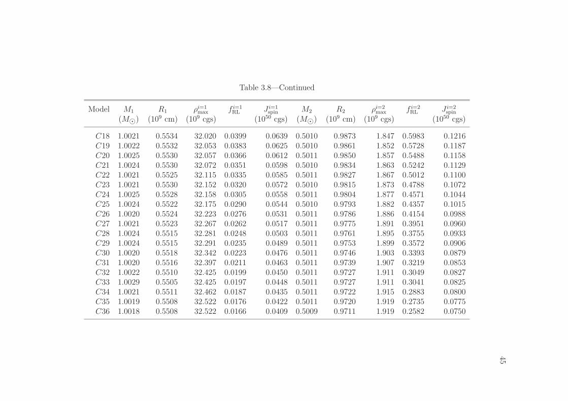
45




max f i=2RL J i=2

spin


C18 1.0021 0.5534 32.020 0.0399 0.0639 0.5010 0.9873 1.847 0.5983 0.1216C19 1.0022 0.5532 32.053 0.0383 0.0625 0.5010 0.9861 1.852 0.5728 0.1187C20 1.0025 0.5530 32.057 0.0366 0.0612 0.5011 0.9850 1.857 0.5488 0.1158C21 1.0024 0.5530 32.072 0.0351 0.0598 0.5010 0.9834 1.863 0.5242 0.1129C22 1.0021 0.5525 32.115 0.0335 0.0585 0.5011 0.9827 1.867 0.5012 0.1100C23 1.0021 0.5530 32.152 0.0320 0.0572 0.5010 0.9815 1.873 0.4788 0.1072C24 1.0025 0.5528 32.158 0.0305 0.0558 0.5011 0.9804 1.877 0.4571 0.1044C25 1.0024 0.5522 32.175 0.0290 0.0544 0.5010 0.9793 1.882 0.4357 0.1015C26 1.0020 0.5524 32.223 0.0276 0.0531 0.5011 0.9786 1.886 0.4154 0.0988C27 1.0021 0.5523 32.267 0.0262 0.0517 0.5011 0.9775 1.891 0.3951 0.0960C28 1.0024 0.5515 32.281 0.0248 0.0503 0.5011 0.9761 1.895 0.3755 0.0933C29 1.0024 0.5515 32.291 0.0235 0.0489 0.5011 0.9753 1.899 0.3572 0.0906C30 1.0020 0.5518 32.342 0.0223 0.0476 0.5011 0.9746 1.903 0.3393 0.0879C31 1.0020 0.5516 32.397 0.0211 0.0463 0.5011 0.9739 1.907 0.3219 0.0853C32 1.0022 0.5510 32.425 0.0199 0.0450 0.5011 0.9727 1.911 0.3049 0.0827C33 1.0029 0.5505 32.425 0.0197 0.0448 0.5011 0.9727 1.911 0.3041 0.0825C34 1.0021 0.5511 32.462 0.0187 0.0435 0.5011 0.9722 1.915 0.2883 0.0800C35 1.0019 0.5508 32.522 0.0176 0.0422 0.5011 0.9720 1.919 0.2735 0.0775C36 1.0018 0.5508 32.522 0.0166 0.0409 0.5009 0.9711 1.919 0.2582 0.0750

46

itemized in Tables 3.3 - 3.8. Along sequence ‘A’ (Figure 3.2), both components of the binary

system are of equal size and display identical degrees of tidal distortion because the mass

ratio q = 1. Along sequences ‘B’ and ‘C’ (Figures 3.3 and 3.4, respectively), however, the

primary star (on the left in each figure panel) is noticeably smaller and less distorted than

the secondary star.

Figure 3.2 Density contours in the equatorial plane are shown for eight separate ZTWDbinary models with increasing separation along inspiral sequence ‘A’ (Mtot = 1.5M⊙; q = 1).Labels in the upper-right-hand corner of each panel identify each model by number accordingto its corresponding position along the sequence as itemized in Tables 3.3 and 3.4.

Figure 3.5 has been constructed from the data detailed in Tables 3.3 and 3.4 for binary

sequence ‘A.’ Specifically, the diamond symbols in the top two panels and in the bottom

panel of this figure show, respectively, how the binary system’s total angular momentum,

Jtot, total energy, Etot, and orbital angular velocity, Ω, vary with orbital separation along

this sequence; and the third panel from the top shows how the Roche-lobe filling factor,

f iRL, varies with orbital separation for both the primary star (diamonds) and the secondary

47

Figure 3.3 Density contours in the equatorial plane are shown for eight separate ZTWDbinary models with increasing separation along inspiral sequence ‘B’ (Mtot = 1.5M⊙; q =2/3). Labels in the upper-right-hand corner of each panel identify each model by numberaccording to its corresponding position along the sequence as itemized in Tables 3.5 and 3.6.

star (asterisks). Figures 3.6 and 3.7 have been similarly constructed from the data detailed,

respectively, in Tables 3.5 and 3.6, and in Tables 3.7 and 3.8.

Following the lead of New & Tohline (1997), in constructing Figures 3.5 - 3.7 we have

normalized our tabulated values of Jtot and Etot to the quantities,

Jnorm ≡ (GM30.75R0.75)

1/2 = 4.0735 × 1050 g cm2 s−1 , (3.2)

Enorm ≡GM2

0.75

R0.75

= 2.0119 × 1050 erg , (3.3)

where R0.75 = 7.4244 × 108 cm is the radius of a spherical ZTWD whose mass is M0.75 =

0.7522 M⊙ as tabulated in Table 3.2. Also, at each separation our tabulated values of Ω

have been normalized to the Keplerian orbital frequency,

ΩK =(

2GM0.75

a3

)1/2

. (3.4)

48

Figure 3.4 Density contours in the equatorial plane are shown for eight separate ZTWDbinary models with increasing separation along inspiral sequence ‘C’ (Mtot = 1.5M⊙; q =1/2). Labels in the upper-right-hand corner of each panel identify each model by numberaccording to its corresponding position along the sequence as itemized in Tables 3.7 and 3.8.

In all three figures, values of the orbital separation have been specified (bottom horizontal

axis) in units of 109 cm and (top horizontal axis) as normalized to the radius of a spherical

ZTWD having the mass of the system’s secondary star as tabulated in Table 3.2, that is,

R0.75 ≡ 7.424 × 108 cm, R0.60 = 8.671 × 108 cm and R0.50 = 9.638 × 108 cm.

New & Tohline (1997) have previously constructed inspiral sequences for equal-mass

DWD binary systems in which the structure of the individual component stars is governed

by the Chandrasekhar ZTWD equation of state (2.1). The sequences published by New &

Tohline (1997) cover a wide range of total masses. The one that most closely resembles our

sequence ‘A’ (our only equal-mass sequence) has Mtot = 1.63M⊙; the functional behavior

of Etot(a) and Jtot(a) for this sequence is presented in Figure 16 of New & Tohline (1997).

Along this Mtot = 1.63M⊙ sequence, the two stars first make contact with their respective

Roche lobes at a normalized separation of approximately 2.825 (see also Figure 5 of New &

49

Tohline 1997). This is completely consistent with the behavior of our sequence ‘A,’ where

contact occurs (model A1) when a/R0.75 = 2.823.

The DWD sequences constructed by New & Tohline (1997) all extend to separations

smaller than the point of first contact, as their SCF technique allowed them to build over-

contact (common envelope) equal-mass binaries. Their functions Etot(a) and Jtot(a) display

a quadratic behavior along the over-contact segment of each sequence, passing through a

minimum at a binary separation smaller than the point of first contact. None of our three

sequences show this behavior because we have not attempted to construct models past the

initial point of contact. Indeed, it seems unlikely that equilibrium configurations exist at

smaller separations except when the system mass ratio is precisely q = 1.

For each of our DWD binary sequences, it is useful to compare the displayed functional

behavior of Jtot(a) from our numerical models against the behavior predicted by two simpli-

fied models. In the case of two point masses in circular orbit, the total angular momentum

Jpm is given simply by the system’s orbital angular momentum, that is,

Jpm = Jorb = M121ΩK + M2

22ΩK

=q

(1 + q)2

[

GM3tota

]1/2

(3.5)

This function, normalized to Jnorm, is displayed by the solid curve in the top panels of Figures

3.5 - 3.7. An even more realistic representation of the function Jtot(a) can be obtained by

adding an approximate representation for the spin angular momentum, IiΩ, of both stars to

the point-mass expression for Jorb. If we assume that both stars retain a spherical structure

while spinning at the Keplerian orbital frequency, ΩK, the appropriate expression for the

total “spinning sphere” system angular momentum is,

Jss = Jorb + (I1 + I2)ΩK = Jorb +(

k1M1R21 + k2M2R

22

)

ΩK

= Jpm

1 +(1 + q)

q

[

k1

(

R1

a

)2

+ qk2

(

R2

a

)2]

, (3.6)

50

where, in addition to q, values of (the constants) Ri and ki appropriate for each binary

sequence can be obtained from Table 3.2. Function (3.6), normalized to Jnorm, is displayed

by the dot-dashed curve in the top panels of Figures 3.5 - 3.7. Analytic expression (3.5)

predicts that Jtot ∝ a1/2. Through a correction factor, Eq. (3.6) displays a somewhat more

complex behavior. Overall, our SCF model sequences match Eq. (3.6) particularly well.

The largest deviation arises in all cases at the smallest separations; the slope of the SCF-

generated Jtot(a) function flattens somewhat as the secondary star approaches contact with

its Roche lobe, that is, as f i=2RL → 1.

The functional dependence of each system’s total energy, Etot(a), can be understood in a

similar fashion. Considering only the kinetic and gravitational potential energy of two point

masses in circular orbit, we obtain,

Eorb = Korb + Worb = −Korb = −1

2

[

q

(1 + q)2

]

GM2tot

a, (3.7)

where we have used the virial relation (2Korb + Worb) = 0. While this a−1 functional depen-

dence explains the general Etot(a) behavior exhibited in Figures 3.5 - 3.7 by our numerically

constructed model sequences, expression (3.7) is missing a nontrivial shift in the overall

energy scale that is set by the binding energies of the two stars, namely,

Eb =2∑

i=1

(

W i + U i)

. (3.8)

Based on the properties of the spherical stellar models provided in Table 3.2, the appropriate

energy shift for sequences ‘A,’ ‘B,’ and ‘C’ is, respectively, Eb = −1.551×1050 ergs, −1.698×

1050 ergs, and −1.963 × 1050 ergs. Adding Eb to Eorb provides what we will refer to as the

“point mass” total system energy,

Epm = −1

2

[

q

(1 + q)2

]

GM2tot

a+ Eb . (3.9)

This analytic function, normalized to Enorm, is displayed as a solid curve in the plots of Etot

versus a shown in Figures 3.5 - 3.7. An improved approximation that we will refer to as

51

the “spinning sphere” total system energy can be obtained by adding the rotational kinetic

energy of both stars, assuming they remain spherically symmetric and spin uniformly with

the Keplerian orbital frequency. Specifically,

Ess = Epm +2∑

i=1

(

1

2IiΩ

2K

)

= Eb + Eorb

1 −(1 + q)

q

[

k1

(

R1

a

)2

+ qk2

(

R2

a

)2]

. (3.10)

This function, normalized to Enorm, is displayed as a dot-dashed curve in the plots of Etot

versus a shown in Figures 3.5 - 3.7. Expression (3.10) describes particularly well the variation

of Etot with separation displayed by our numerically constructed binary sequences ‘B’ and

‘C.’ We note, however, that all three of our sequences show that the total system energy

drops slightly below the behavior predicted by Eq. (3.10) at the smallest separations.

The curve outlined by asterisks in the third panel from the top of Figures 3.5 - 3.7 shows

that f i=2RL steadily increases from a value ∼ 0.2 to a value of 1.0 at the smallest separation

along all three inspiral sequences, implying that the secondary star has made contact with

its Roche lobe. For comparison, the curve outlined by diamonds in the same panel of these

three figures shows how the Roche-lobe filling factor of the primary star varies along each

sequence. The value of f i=1RL does not climb above 0.063 for sequence ‘C’ or above 0.191

for sequence ‘B,’ reflecting the fact that in both cases the primary star is significantly more

massive — and, hence, it has a significantly smaller radius — than the secondary star. For

inspiral sequence ‘A,’ f i=1RL (a) displays an identical behavior to f i=2

RL (a) because the primary

and secondary stars have equal masses.

The bottom panel of Figures 3.5 - 3.7 displays the behavior of the normalized orbital

frequency Ω/ΩK as a function of binary separation derived from our three numerically con-

structed inspiral sequences. At the smallest separations, our models show that the orbital

frequency is always ∼ 0.5% higher than predicted by the “point-mass” Keplerian frequency.

Our equal-mass sequence exhibits the largest deviation at contact; specifically, for model

52

‘A1,’ we find Ω = 1.0085 ΩK. As the separation is increased along each sequence, the figures

show that Ω/ΩK approaches unity, as expected. However, at a sufficiently wide separation,

each of our sequences displays a tiny discontinuous drop in the orbital frequency, followed

by further decline that ultimately falls below the local Keplerian value. We suspect this odd

behavior at wide separations arises from the discrete nature of our grid calculations cou-

pled with progressively fewer grid zones falling inside both stars — resulting in progressively

poorer numerical resolution — at wider separations.

3.2 Contact Sequences

During a phase of stable mass transfer, a DWD binary system will evolve in such a way

that the secondary star remains in marginal contact with its Roche lobe while it slowly

transfers mass to the primary star. If the total mass of the system is conserved, then the

evolution should proceed along a sequence of synchronously rotating configurations in which

Mtot is constant, f i=2RL = 1, and q is steadily decreasing. Models A1, B1 and C1 can be

viewed as representing three such configurations along a sequence whose total system mass

is Mtot = 1.5M⊙. In evolving from an initially equal-mass, contact configuration (model

A1) to a semi-detached configuration with q = 2/3 (model B1), then on to a semi-detached

configuration with q = 1/2 (model C1), the separation of such a system (measured in units

of 109 cm) will increase from a9 = 2.10, to a9 = 2.67, then to a9 = 3.18; and the system’s

orbital period (Porb = 2π/Ω) will increase from 42.3 s to 61.0 s, then to 79.5 s.

It is clear, therefore, that our new SCF code can be used to construct model sequences

that mimic the evolution of DWD systems undergoing slow, conservative mass-transfer. The

models detailed in Tables 3.9 (sequence ‘D’) and 3.10 (sequence ‘E’) trace two such semi-

detached sequences as the system mass ratio evolves from q = 1 to q ∼< 0.5. For sequence

‘D,’ Mtot = 1.5M⊙ and for sequence ‘E,’ Mtot = 1.0M⊙. In the top two panels of Figures 3.8

and 3.9, data from Tables 3.9 and 3.10 have been plotted as diamond symbols to illustrate

53

Table 3.9. Semi-detached DWD Sequence ‘D’; Mtot = 1.5M⊙

Mtot q a Ω Jtot Etot VE(M⊙) (109 cm) (10−2 s−1) (1050 cgs) (1050 erg)

1.5048 1.0000 2.1010 14.8472 5.3866 −1.8636 1.5 × 10−4

1.5034 0.9508 2.1638 14.1787 5.4116 −1.8566 1.8 × 10−4

1.5045 0.8994 2.2336 13.4444 5.4491 −1.8611 9.5 × 10−5

1.5034 0.8507 2.3102 12.8287 5.4797 −1.8628 1.4 × 10−4

1.5033 0.8007 2.3961 12.1414 5.5141 −1.8736 2.2 × 10−4

1.5034 0.7504 2.4919 11.4431 5.5460 −1.8925 3.1 × 10−4

1.5034 0.7004 2.5987 10.7442 5.5702 −1.9194 4.0 × 10−4

1.5034 0.6504 2.7188 10.0382 5.5871 −1.9572 5.5 × 10−4

1.5032 0.6004 2.8550 9.3217 5.5914 −2.0072 7.2 × 10−4

1.5033 0.5503 3.0109 9.0670 5.5804 −2.0741 9.1 × 10−4

1.5031 0.5004 3.1914 7.8907 5.5484 −2.1587 1.2 × 10−3

how a and Ω vary with q while f i=2RL is held to a value of unity (definition of a semi-detached

binary) along these two fixed-mass sequences.

Up to now, the community has relied upon some relatively simple analytic expressions

to approximate the behavior of, for example, a(q) along conservative mass-transfer evolu-

tionary trajectories. For example, by setting the radius of the secondary star as given by

the Nauenberg mass-radius relation (A.14) equal to the Roche-lobe radius RRL as defined in

terms of a and q by the approximate relation provided by Eggleton (1983), namely,

RRL = a[

0.49q2/3

0.6q2/3 + ln(1 + q1/3)

]

, (3.11)

one obtains,

a

R⊙

≈ 0.0229(n2q2)−1/3(1 − n

4/32 )1/2

[

0.6q2/3 + ln(1 + q1/3)]

, (3.12)

where,

n2 ≡q

(1 + q)

(

Mtot

Mch

)

. (3.13)

54

Table 3.10. Semi-detached DWD Sequence ‘E’; Mtot = 1.0M⊙

Mtot q a Ω Jtot Etot VE(M⊙) (109 cm) (10−2 s−1) (1050 cgs) (1050 erg)

1.0030 1.0000 2.7109 8.2477 3.3579 −0.6657 1.7 × 10−4

1.0024 0.9504 2.7778 7.9369 3.3687 −0.6642 1.6 × 10−4

1.0019 0.9001 2.8641 7.5710 3.3850 −0.6636 2.1 × 10−4

1.0022 0.8508 2.9380 7.2829 3.3983 −0.6659 2.2 × 10−4

1.0024 0.8003 3.0161 6.9993 3.4073 −0.6698 2.2 × 10−4

1.0024 0.7503 3.1165 6.6609 3.4163 −0.6751 2.6 × 10−4

1.0024 0.7003 3.2294 6.3129 3.4212 −0.6828 3.3 × 10−4

1.0023 0.6502 3.3569 5.9551 3.4204 −0.6934 3.9 × 10−4

1.0023 0.6003 3.5026 5.5862 3.4123 −0.7074 4.7 × 10−4

1.0022 0.5503 3.6696 5.2078 3.3943 −0.7254 5.6 × 10−4

1.0021 0.5003 3.8649 4.8169 3.3644 −0.7484 6.8 × 10−4

1.0020 0.4504 4.0955 4.4134 3.3184 −0.7773 8.0 × 10−4

The function a(q), defined by Eq. (3.12) for a given Mtot, has been plotted as a solid curve

in the top panels of Figures 3.8 and 3.9, and the Keplerian orbital frequency associated with

this separation (and relevant Mtot) has been plotted as a solid curve in the second panel

of Figures 3.8 and 3.9. For both sequence ‘D’ and sequence ‘E,’ the analytically derived

curves are consistently offset by 3 - 5% from our numerical model results. But overall, the

analytically predicted functional behavior of a(q) and Ω(q) is in very good agreement with

our results. This is reassuring as it provides a degree of validation for both our numerical

code and the approximations that were adopted by earlier investigators when deriving the

more easily manipulated analytic expressions.

Finally, in the bottom two panels of Figures 3.8 and 3.9, the diamond symbols display the

variation of Jtot and Etot with q along sequence ‘D’ and sequence ‘E,’ respectively. The solid

curve drawn in the Jtot(q) panel of both figures shows the behavior predicted by our “spinning

sphere” expression for the total system angular momentum (3.6) when used in conjunction

55

with the a(q,Mtot) behavior prescribed by Eq. (3.12). Again, for a given Mtot there appears to

be very good agreement between the functional behavior of Jtot(q) displayed by our numerical

model results and the analytic expressions. There is also a systematic offset between the

two. In either case it is clear that, unlike the behavior displayed by a(q) and Ω(q), the

system’s total angular momentum does not vary monotonically with q along a conservative

mass-transfer evolutionary trajectory. Note, in particular, that if the system mass ratio q is

initially close to unity, Jtot increases as q decreases along the displayed trajectory. This result

is unphysical. It signifies that slow evolution along a synchronously rotating, conservative

mass-transfer trajectory can occur only if, at the onset of mass-transfer, q < qcrit, where the

value of qcrit for a given Mtot is prescribed by the location of the maximum of the Jtot(q)

curve. For our model sequences ‘D’ and ‘E,’ we see that qcrit ∼< 2/3, consistent with the

mass-transfer stability limit that has already received much attention in the literature.

56

Figure 3.5 (Top panel) Normalized total angular momentum, Jtot/Jnorm, (second panel) nor-malized total energy, Etot/Enorm, (third panel) the Roche-lobe filling factor, fRL, for thesecondary (asterisks) and primary (diamonds) stars, and (bottom panel) the normalized or-bital angular velocity, Ω/ΩK, are plotted as a function of binary separation for models A1through A35 along inspiral sequence ‘A’ (Mtot = 1.5M⊙; q = 1). Data for the individualmodels is drawn from Tables 3.3 and 3.4; the separation a is labeled in units of 109 cm alongthe bottom axis and as a ratio to R0.75 along the top axis. The solid curves in the top twopanels display the analytic functions Jpm(a)/Jnorm and Epm(a)/Enorm given, respectively, byEqs. (3.5) and (3.9) for a “point-mass” sequence of the specified total mass and mass ra-tio; and the dot-dashed curves display the analytic functions Jss(a)/Jnorm and Ess(a)/Enorm

appropriate for a “spinning spheres” sequence given, respectively, by Eqs. (3.6) and (3.10).

57

Figure 3.6 Same as Fig. 3.5 but for models B1 through B49 along the inspiral sequence‘B’ (Mtot = 1.5M⊙; q = 2/3), as tabulated in Tables 3.5 and 3.6; along the top axis, theseparation a is labeled as a ratio to R0.60.

58

Figure 3.7 Same as Fig. 3.5 but for models C1 through C36 along the inspiral sequence‘C’ (Mtot = 1.5M⊙; q = 1/2), as tabulated in Tables 3.7 and 3.8; along the top axis, theseparation a is labeled as a ratio to R0.50.

59

Figure 3.8 System parameters a, Ω, Jtot, and Etot at contact as a function of mass ratio,q, for DWD systems having a total mass of 1.5M⊙. Solid curves in the top three panelsshow predicted behavior based on Nauenberg’s (1972) and Eggleton’s (1983) approximate,analytic expressions as discussed in the text.

60

Figure 3.9 Same as Figure 3.8, but for DWD systems having a total mass of 1.0M⊙.

4. Hydrodynamic Techniques

There are two different philosophies for implementing numerically evolving hydrodynam-

ics. In the first the fluid is divided into parts, and individual components or particles of

the fluid are tracked as they move through space. This approach is called the Lagrangian

method and is the method used in the SPH simulations described in Section 1.5. In the

second technique the region of interest is divided into a grid. The fluid values are defined

for each cell on the grid and the fluid is evolved by advecting it through the grid. This

grid based approach is the Eulerian method. Both the Lagrangian and Eulerian methods

have advantages and disadvantages that need to be considered when selecting the better

method for the problem to be solved. The Lagrangian method only tracks the fluid particles

making it useful if you have voids in the simulation where there is little to no fluid because

no computational time is used on these regions since there are no particles. However, the

minimally resolvable density of the fluid is directly related to the number of particles used

in the simulation. The Eulerian method must spend an equal amount of computational time

on each cell regardless of the amount of fluid in the cell, even if it contains no fluid. If the

problem does not match the chosen grid well, this can lead to large inefficiencies in the code

from calculating areas of little physical interest. Since the Eulerian approach assigns scalar

densities in all cells, the minimally resolvable density in a region is not tied to the number

of cells, hence a greater range of densities can be covered in an Eulerian simulation than

in the Lagrangian method. In the mass transferring DWD simulations the density of the

material in the stream between the stars is many orders of magnitude lower than the central

densities of the star, especially for the initial stream at the onset of mass transfer. By using

the Eulerian method, we hope to be able to do more accurate simulations of the stream than

61

62

have been done with previous Lagrangian codes and therefore allow the system to evolve

more slowly into the mass transfer.

4.1 Summary of Hydrodynamics Code

Our hydrodynamics code is a 3D explicit Eulerian hydrodynamics code developed principally

by Patrick Motl. A detailed description of the code can be found in Motl (2001), Motl et

al. (2002) and D’Souza et al. (2006). The code is implemented on a fixed uniform cylindrical

grid, with the option of conducting the simulation in a rotating frame. Scalar quantities are

defined on cell centers and vector quantities are defined on cell faces. The code tracks the

following fluid quantities: density, ρ; angular momentum density, Am; vertical momentum

density, Tm; radial momentum density, Sm; and the entropy tracer, τ . The entropy tracer is

defined in terms of the internal energy per unit mass, ǫ, the density, and the ratio of specific

heats, γ by the expression,

τ ≡ (ǫρ)1

γ . (4.1)

In a later modification to the code the total energy density, E, is also tracked. The grav-

itational potential is calculated using a Fast Fourier Transform that reduces the Poisson

equation to a group of independent 2D Helmholtz equations that are then solved using an

alternating direction implicit (ADI) solver. The boundary conditions are calculated using

the compact cylindrical Green’s function expansion described in Cohl & Tohline (1999).

The main physical equations used to advance the simulation are:

∂ρ

∂t+ ρ~∇ · ~v = 0 (4.2)

∂Sm

∂t+ ∇ · (Sm~v) = −

∂P

∂− ρ

∂Φeff

∂+

A2m

ρ3+ 2Ω

Am

(4.3)

∂Tm

∂t+ ∇ · (Tm~v) = −

∂P

∂z− ρ

∂Φeff

∂z(4.4)

∂Am

∂t+ ∇ · (Am~v) = −

∂P

∂θ− ρ

∂Φeff

∂θ− 2ΩSm (4.5)

63

∂τ

∂t+ ~∇ · (τ~v) = 0 (4.6)

Φeff = Φ −1

2Ω22 (4.7)

∇2Φ = 4πGρ, (4.8)

where Eq. (4.2) represents mass conservation, Eq. (4.3) - Eq. (4.5) represent conservation

of the three momentum components, Eq. (4.6) is the energy conservation equation for an

adiabatic fluid, Eq. (4.7) is the definition of the effective potential in the rotating frame,

Φeff , and Eq. (4.8) couples the gravitational potential through the Poisson equation to the

density. These equations are implemented numerically using second order accurate methods.

For additional details and tests of the code see Motl (2001).

4.2 Zero Temperature Equation of State

The hydrodynamics code, hereafter hydrocode, was initially implemented for a polytropic

equation of state (EOS). The polytropic EOS is defined as

P = κρn+1/n = κργ (4.9)

where κ is constant and n is the polytropic index. In the literature, n=3/2 polytropes are

often used to approximate white dwarf structures. As shown in the top right panel of Figure

1.1, this may be acceptable for low-mass white dwarfs. The polytropic EOS is useful because

it is simple to implement and allows scaling to different physical values after the calculation.

However, there are weaknesses in using polytropes. The polytropic EOS does not enforce

the proper mass-radius relation for white dwarfs and solutions with the more massive star

being larger in radius than the less massive star are acceptable solutions to the polytropic

EOS. Implementing a ZTWD EOS allows for more physically realistic DWD binaries to

be investigated. We have implemented the ZTWD EOS into the current version of the

hyrdrocode through a series of relatively minor changes. In the original version the pressure

64

for the polytropic gas was calculated from the entropy tracer. The use of the entropy tracer

can be removed and the pressure can be calculated directly from the density using Eq. (2.1).

Extra care must be taken to ensure that the hydrocode and SCF code are using the same

normalizations for the dimensionless units used in the two codes. Additionally, the way the

speed of sound is calculated needs to be updated to account for the new equation of state.

The sound speed is used to calculate the maximum size of the timestep that will yield stable

solutions. The adiabatic sound speed, cs, is defined as,

c2s =

∂P

∂ρ. (4.10)

Evaluating Eq. (4.10) using Eq. (2.1) for the pressure, the sound speed is shown to be,

c2s =

8A

3B

(

ρB

)2

3

[

1 +(

ρB

)2

3

]

1

2

=8A

3B

x2

[1 + x2]1

2

. (4.11)

The zero temperature equation of state is based on the assumption that the degeneracy

pressure is significantly greater than the thermal pressure of the gas. In the initial equilibrium

models this is a valid assumption. However, the accreting fluid can reach supersonic speeds

as it approaches the surface of the accreting star. This will create shocks as it impacts the

surface. These shocks generate large amounts of thermal energy, creating regions where the

initial assumption may break down and the degeneracy pressure is no longer much greater

than the thermal pressure. To solve this we will track two pressures, the degeneracy pressure,

Pdeg, and a thermal gas pressure, Pgas.

The fluid in the simulation is modeled using a combination of a zero-temperature Fermi

fluid and an ideal gas. The total pressure, P , is the sum of pressure from the zero-temperature

fluid, Pdeg, and the ideal gas, Pgas. The zero temperature white dwarf equation of state gives

the electron degeneracy pressure Pdeg as a function of only the density, ρ, by the relation in

Eq. (2.1). The internal energy density of the degenerate electron gas, Edeg, is given by the

65

relation,

Edeg = A[

8x3(

(x2 + 1)1/2 − 1)

−(

x(2x2 − 3)(x2 + 1)1/2 + 3 sinh−1 x)]

, (4.12)

as described in (Benz et al., 1990). Additionally, the kinetic energy density of the gas, Ek,

in the rotating frame can be defined as

Ek =1

2ρv2, (4.13)

where v is the velocity in the rotational frame. The total energy density of the fluid, E, is

defined as

E = Edeg + Egas + Ek, (4.14)

where Egas is the internal energy density of the ideal gas component of the fluid. Initially

Egas and Pgas are set to zero and E can be calculated directly from ρ and ~v. Conservation

of energy is given by

∂E

∂t+ ∇ · (E~v) = −∇ · (P~v) − ρ~v · ∇Φeff . (4.15)

The second term on the left is treated in the advection subroutine. The right hand side

terms are then updated in the source subroutine through,

En+1 = En −(

∇ · (P~v) + ρ~v · ∇Φeff

)

δt. (4.16)

where En is the current value of energy density, En+1 is the value being calculated, and δt

is the time step size between the two iterations. The discrete form of the derivatives in Eq.

(4.16) are

∇ · (p~v) =1

d

[(

PSm

ρ

)

+ 1

2

−(

PSm

ρ

)

− 1

2

]

(4.17)

+1

dθ

[(

PAm

ρ

)

θ+ 1

2

−(

PAm

ρ

)

θ− 1

2

]

+1

dz

[(

PTm

ρ

)

z+ 1

2

−(

PTm

ρ

)

z− 1

2

]

66

and

ρ~v · ∇Φeff =1

4d

[(

Sm)

+ 1

2

+(

Sm)

− 1

2

][

Φ+1eff − Φ−1

eff

]

(4.18)

=1

4dz

[(

Tm

)

z+ 1

2

+(

Tm

)

z− 1

2

][

Φz+1eff − Φz−1

eff

]

=1

42dθ

[(

Am

)

θ+ 1

2

+(

Am

)

θ− 1

2

][

Φφ+1eff − Φφ−1

eff

]

.

With updated values of E, Edeg, and Ek, the internal energy density of the ideal gas, can be

calculated from Equation (4.14) as

Egas = E − Edeg − Ek. (4.19)

The pressure of the polytropic component of the gas, Pgas, is defined as

Pgas = (γ − 1)Egas. (4.20)

An additional factor is added to Eq. (4.20) to eliminate spurious effects from developing and

dominating the behavior in the low density regions. These effects can develop since Egas is

initially derived from the difference of nearly identical numbers and its accuracy is limited

by machine precision. In practice, the value of Pgas in the simulation is calculated through

the relation

Pgas = (γ − 1)Egas

[

1 −ρp

ρ

]

for ρ ≥ ρp

Pgas = 0 for ρ < ρp (4.21)

where ρp/ρ∗ is defined to be 10−8 in the simulations presented in Chapter 5. The value of

ρp/ρ∗ was chosen by weighing the accuracy of the solution gained versus the reduction in

timestep size required.

Table 4.1 displays the timestep size for 3 values of ρp/ρ∗: 10−7, 10−8, and 10−9. The

average timestep in the table is calculated for between approximately 0.25 and 0.35 orbital

periods. The first column indicates the value of ρp/ρ∗ used in the simulation, the second

67

column is the final timestep used in the calculation, the third is the time at the final timestep,

the fourth and fifth columns are the initial timestep and time, and the final column shows

the average value of the timestep over the 0.1 orbit interval. The three simulations were

all conducted with identical initial conditions and with all parameters in the code identical

except ρp/ρ∗ was varied. The reduction in timestep between the first two is less than a factor

of 2. When ρp/ρ∗ is reduced by another order of magnitude, the timestep size is reduced by

a factor of 5. This is a significant amount of additional time and will limit the number of

orbits that are possible to run in a simulation. Figure 4.1 displays the value and time rate of

change of the binary separation, a, as a function of time. Figure 4.2 displays the time rate

of change of the total angular momentum and the value of central density of the accretor

as a function of time for the simulations identified in Table 4.1. The values of the plotted

quantities vary significantly when changing between ρp/ρ∗ of 10−7 and 10−8. The plots for

10−8 and 10−9 show much better agreement in all quantities. The close agreement between

results when ρp/ρ∗ = 10−8 and ρp/ρ∗ = 10−9 and the increase of a factor of 5 in time led

to the choice of ρp/ρ∗ being 10−8. Figure 4.3 shows the density (left) and pressure (right)

contours at a time of t/Po=0.4 for the 3 test simulations. The most obvious difference is in

the ρp/ρ∗ = 10−9 case where, in the extremely low density regions, ρ < 1g/cm3, the pressure

is dominated by the thermal pressure that is absent in the other two cases.

Finally, the total pressure of the fluid is then calculated as a sum of the two individual

pressures,

P = Pgas + Pdeg. (4.22)

The temperature, T, of the gas can be calculated from Pgas using the ideal gas law giving,

T =Pgasµ

ρℜ, (4.23)

where µ is the mean molecular weight and ℜ is the gas constant (8.3145×107 erg/deg · mol).

68

Table 4.1 Variation of timestep size with ρp/ρ∗

ρp/ρ∗ Timestep Orbits Timestep Orbits Average Timestep10−7 56800 0.3458 45300 0.2453 8.73133 × 10−6

10−8 60400 0.3460 43300 0.2460 5.84299 × 10−6

10−9 323600 0.3458 237900 0.2458 1.1668 × 10−6

Figure 4.1 Top: The binary separation normalized to the initial separation as a function oftime in orbital periods for a q=2/3 simulation. The three curves represent simulations runwith identical conditions except that the value of ρp/ρ∗ was varied to the value specified in thelegend. Bottom: The time variation of the normalized separation for the same simulationsin the top.

69

Figure 4.2 Same simulations as Figure 4.1. Top: Time variation of the total angular momen-tum normalized to the initial angular momentum. Bottom: The value of the central densityof the accretor normalized to the initial central density.

70

Figure 4.3 Equatorial slices of the simulations in Figures 4.1-4.2 0.4 orbital periods into thesimulations. Top Row: The left image is the density contour in the equatorial plane in g/cm3

for ρp/ρ∗ of 10−7. The right image is the pressure in dyne/cm2 for the same ρp/ρ∗. MiddleRow: Same as above except ρp/ρ∗ equals 10−8. Bottom Row: Same as above except ρp/ρ∗

equals 10−9.

5. Binary Merger Simulations

5.1 Previously Published Hydrocode Simulations

In D’Souza et al. (2006) and Motl et al. (2007) the stability of mass transfer in the binary

systems is investigated using an n = 3/2 polytropic equation of state and the same hydrody-

namics code used in this work. Direct impact accretion in systems with initial mass ratios of

q= 1.3 and 0.5 are investigated in D’Souza et al. (2006), and Motl et al. (2007) examine the

q=0.4 case. In these simulations nearly equilibrium initial conditions were created and the

systems were driven into Roche lobe over fill. This driving was done by removing a small

amount of angular momentum from each cell at each time step. The amount removed was

set so that the angular momentum decreased at a constant rate, 1% per orbit being typical.

The driving was then stopped once a desired level of contact is reached.

In the simulations q=1.3, after the initial driving was stopped, the mass transfer rate

continued to grow throughout the simulation until the donor was tidally disrupted after

12 orbits. An initial binary system with a mass ratio of q=0.5 was evolved with several

different driving rates. D’Souza et al. (2006) demonstrated that varying the level of Roche

lobe overflow created by driving can substantially change the outcome of the system. The

simulations were all driven at 1.0% for 2.7 orbits and then the driving was cut off immediately

for case A, continued until 5.3 orbits for case B, and the driving was continued throughout

for case C. In cases A and B, the mass transfer system underwent a period during which the

binary separation remains steady and the mass transfer rate changes slowly. Eventually the

separation increased and the system could no longer be followed due to numerical limitations

of the grid. However, these periods of relatively stable mass transfer lasted for on the order

of 10 orbits in case B and 30 orbits in case A. In the constantly driven case C, the mass

71

72

transfer rate increased throughout the simulation until the donor was disrupted in 8.5 orbits.

In Motl et al. (2007) a system with an initial mass ratio of q=0.4 was driven at a rate of

1% for 1.16 orbits. In this case the mass transfer rate increased for the first 10 orbits and

then began to decrease and leveled off to a constant rate at around 30 orbits. This system

was followed through over 40 orbits with no indication that a merger or tidal disruption was

imminent.

These results indicate that stable - or at least more slowly evolving - mass transfer than

was seen in the previous SPH simulations is possible with a near equilibrium initial condition.

However, the previous polytropic simulations with the hydrocode were done at significantly

different mass ratios than the mass ratio in the published SPH simulations of DWDs.

5.2 q = 0.7 Polytrope

We have carried out a series of polytropic simulations to better compare the zero temperature

equation of state results with polytropic results. The 3 polytropic simulations were all started

with an identical initial state with a mass ratio of q=0.7. The first two simulations, Q0.7a

and Q0.7b, were conducted using the same version of the hydrocode that was used in D’Souza

et al. (2006) and in Motl et al. (2007), but with different initial conditions. The Q0.7a system

was driven at a rate of 1% for 2.28 orbits. The density in the equatorial plane at 6 different

times is shown in Figure 5.1. Plots of global scalar quantities and their derivatives are shown

in Figures 5.2 - 5.5 for Q0.7a, Q0.7b, and Q0.7c.

As shown in Figure 5.3 by the blue curves, after the driving is stopped in the Q0.7a

evolution, the binary separation steadily decreases as the mass transfer rate increases for

10 more orbits. During this time the angular momentum of the accretor (middle panel of

Figure 5.4) is increasing as infalling donor material spins it up. After 12 orbits the separation

decreases and mass transfer rate increases quickly as the donor is tidally disrupted and forms

a thick disk around the accretor. In order to investigate whether the driving pushed the

73

system too far into contact for the system to have a chance to recover, as seen in some of the

simulations in D’Souza et al. (2006), the system was restarted and driven for only 1.7 orbits

in case Q0.7b (gold curves in Figures 5.2-5.5). As shown in Figure 5.5, this reduced the mass

transfer rate by an order of magnitude between Q0.7a and Q0.7b within 1 orbital period after

the driving was stopped. However, the mass transfer rate increased steadily while the binary

separation decreased. After approximately 10 orbits the mass transfer rate reaches the rate

initially present in Q0.7a. After this time, Q0.7b evolves almost identically to Q0.7a with an

8 orbit time shift. This supports the conclusion that for a system with q=0.7 initially, mass

transfer is dynamically unstable and a merger/tidal disruption will result if mass transfer is

begun regardless of the depth of initial contact.

The third case, Q0.7c, has identical driving to Q0.7a, but has a modified EOS that

incorporates an ideal gas that can be heated through shocks. The addition of this heating

creates a low density common envelope around the binary during the phase of mass transfer.

The addition of this common envelope results in a higher mass transfer rate (red curves in

Figure 5.5) in the early orbits and leads to the system merging somewhat sooner (red curves

in Figure 5.3), but still in the same qualitative way as in Q0.7a and Q0.7b. All 3 polytropic

simulations indicate that a DWD binary with a mass ratio of q=0.7 will result in a tidal

disruption of the donor, although the system can survive in a mass transferring state for

many orbits if the initial conditions are close enough to equilibrium and if the system is not

driven too far into contact initially.

5.3 q = 2/3 Zero Temperature

The first hydrodynamic run using an initial model from the SCF code with a zero temperature

EOS was conducted using the same EOS as presented in the SCF code. Model B3 (Mtot=1.5

M⊙) from chapter 3.1 served as the initial model for this evolution which will hereafter be

referred to as evolution Q2/3a. This ZTWD EOS only accounts for the electron

74

Figure 5.1 Mass density in the equatorial plane for simulation Q0.7a, an n=3/2 binary systemwith an initial mass ratio q=0.7. The binary is initially just beyond semi-contact and hasangular momentum removed at 1% per orbit for 2.28 orbits to begin mass transfer. The masstransfer rate grows slowly until the last couple of orbits when the donor is tidally disruptedand a core-disk structure is created.

75

Figure 5.2 Top: The mass of the accretor vs. time for 3 different polytropic binary evolutionswith an initial mass ratio of q=0.7. The mass is normalized to the initial mass and the timeis displayed in orbital periods of the initial binary system. Middle: Mass of the donornormalized to the initial donor mass. Bottom: Mass ratio of the donor to accretor, q.

76

Figure 5.3 Top: The binary separation vs. time for 3 different polytropic binary evolutionswith an initial mass ratio of q=0.7. The separation is normalized to the initial separationand the time is displayed in orbital periods of the initial binary system. Bottom: Totalangular momentum of the binary system normalized to the initial value.

77

Figure 5.4 Top: The orbital angular momentum vs. time for 3 different polytropic binaryevolutions with an initial mass ratio of q=0.7. The orbital momentum is normalized to theinitial total momentum and the time is displayed in orbital periods of the initial binarysystem. Middle: The spin angular momentum of the accretor normalized to the initial totalangular momentum. Bottom: Spin angular momentum of the donor normalized to the initialtotal angular momentum.

78

Figure 5.5 Top: The time rate of change of the mass of the accretor for 3 different polytropicbinary evolutions with an initial mass ratio of q=0.7. The mass transfer rate is displayed inunits of total mass of the binary per orbital period and time is displayed in initial orbitalperiods. Bottom: The time rate of change of the mass of donor.

79

degeneracy pressure and therefore pressure is only a function of density and has no temper-

ature dependence. This simulation corresponds closely to the purely polytropic evolutions

Q0.7a and Q0.7b described in §5.2. This model leaves out a substantial amount of physics

that could have a large impact on the structure of the final merged object, but it provides

a good starting point to examine the dynamics of the mass transfer and compare with the

polytropic results.

Figure 5.6 shows the density in the equatorial plane at 6 different points in time during the

Q2/3a evolution. The evolution was initially driven at 1% for 2.25 orbits and then continued

with no driving. During the first 8 orbits the system slowly develops a mass transfer stream.

The stream slowly increases in density and thickness and during this period. The structure

of the donor and accretor change very little, with the exception of a small mound forming on

the accretor where the stream is impacting. Around 10 orbits the donor begins to develop

noticeable distortions on its surface. As shown in the upper right-hand panel of Figure 5.6,

for example, the accretor has devoloped a clear triangle distortion. The blue curve in Figures

5.12 to 5.16 plot global scalar quantities as a function of time for evolution Q2/3a. In Figure

5.16 it is seen that, during the time when the surface distortions appear on the donor, the

mass transfer rate begins to level off, suggesting that these surface waves feed back into the

binary system and affect the eventual outcome. Around 15 orbits, the mass transfer begins

to increase again and by 18 orbits the donor tidally disrupts. This final state is qualitatively

very similar to evolutions Q0.7a and Q0.7b. When the donor tidally disrupts at 18 orbits,

the donor material forms a thick disk around the accretor with the accretor surviving without

any drastic changes to its structure.

The blue curve in the top panel of Figure 5.15 shows that during the merger the central

density of the accretor increases by 40%. The bottom panel of Figure 5.15 shows the mass

of an isolated white dwarf with a central density equal to the value in the upper panel. The

change in central density during the merger would have corresponded to approximately a

80

6% increase in mass of an isolated white dwarf. However the mass in the core/disk system

is significantly higher than the initial 0.9 M⊙ present in the accretor. This additional mass

has only a small effect on the central density and the core because it is largely rotationally

supported. After the merger, the system is evolved through several more orbital periods until

the disk settles into a structure that is approximately symmetric in the azimuthal direction.

In Figure 5.7 the azimuthally averaged density in the equatorial plane is plotted as a function

of radial distance from the center. Figure 5.8 shows the same azimuthally averaged density

as Figure 5.7, but displayed as a meridional (, z) plane contour plot to examine the vertical

structure of the system. A distinct high density core with a value that declines rapidly with

radial distance out to a r ≈ 5× 108 can be seen along with a lower density disk in which the

density tapers off more slowly. The central core remains nearly spherical with no additional

vertical structure above it and the disk has a thickness approximately equal to the diameter

of the core. Figure 5.9 displays the angular frequency of the azimuthally averaged material

in the equatorial plane as a fraction of the Keplerian frequency. The Keplerian frequency is

defined as

ΩK ≡

√

1

dΦ

d, (5.1)

where Φ is the azimuthally averaged gravitational potential. A ratio of 1 for the frequency

to the Kepler frequency would represent material that is completely rotationally supported.

The lower the ratio, the greater part the gas pressure plays in maintaining the structure.

In the region that corresponds to the peak in the density, the ratio of frequencies is very

small dropping to almost zero at the center. This indicates that the central object is almost

entirely pressure supported. In the disk region the ratio is 0.8, indicating that the rotational

support of this material is preventing it from further compressing onto the core. Given

enough time, various effects could remove angular momentum from the disk and cause it to

81

accrete onto the central core, but the time scale for this is longer than can be carried out by

these computationally expensive simulations.

5.4 q = 2/3 Zero Temperature Plus Ideal Gas

In the extremely high density region in the interior of the white dwarf, the electron degen-

eracy pressure will dominate over the thermal pressure of the gas even at extremely high

temperatures, allowing the zero temperature approximation to be a useful tool for many

systems. However, the thermal pressure will begin to dominate in the low density and high

temperature regions on the surface of the stars and in the void between them. The accretion

stream is a low density feature that greatly affects the eventual outcome of the binary sys-

tem and adding the thermal pressure is a crucial step in obtaining more physically realistic

results for the DWD mass transferring systems. Here, the initial system from §5.3 is run

again with the same driving, but using the modified equation of state to include heating

through shocks, as described in §4.2. This evolution will be referred to as Q2/3b.

Figures 5.10 and 5.11 show the density (left) and temperature (right) distributions in the

equatorial plane at 6 times throughout the Q2/3b evolution. In the top panel of Figure 5.10

it should be noted that the temperature everywhere is initially zero because the simulation

is started from a zero temperature approximation from the SCF calculation. Comparing the

density contours in Figures 5.10 and 5.11 with the ones presented in Figure 5.6, the most

obvious visual difference is the presence of a low density common envelope when heating is

added (evolution Q2/3b) that is completely absent in the zero temperature case (evolution

Q2/3a). In the left-middle frame of Figure 5.10, the higher density component of the accre-

tion stream has a density and thickness very similar to the accretion stream in the second

panel of Figure 5.6. However, an envelope of material several times thicker than the stream

with a density 1-100 g/cm3 surrounds the stream. This 1-100 g/cm3 feature isn’t present in

Figure 5.6 as the density drops from 103 g/cm3 to below 1 g/cm3 within a couple of grid

82

cells. In addition, the well-defined surface waves seen in the zero temperature case are absent

when the ideal gas component is added. In the third panel of Figure 5.6, a clear triangular

structure is seen in the accretor at 12.5 orbits and this additional structure is destroyed by

16.6 orbits when the donor begins to tidally disrupt as seen in the fourth frame. In the

middle and bottom rows of Figure 5.10 there is no indication of additional structure on the

donor, and even the bulge that formed where the accretion stream impacted the donor that

is seen in Figure 5.6 is absent. However, the higher density structure in the two simulations

is qualitatively similar in the two cases. The density contours in Figure 5.11 and the last 3

frames of Figure 5.6 show that the disruption of the donor is qualitatively very similar in

the two simulations.

The temperature of the core of the accretor and the entire donor remain at or below

107 K throughout the entire Q2/3b simulation, even during the disruption and merger.

The extremely low density gas that fills the void between the stars and the spot were the

accretion stream impacts the accretor are the hottest locations. The gas heated at the base

of the accretion stream eventually flows around the accretor creating a hot outer layer that

is slowly diffusing further into the core of the donor. This increase in temperature provides

additional pressure support for the accretor and, despite matter being added, as the gold

curves in Figure 5.15 show, the central density of the accretor actually decreases by 10%

during the phase of mass transfer. During the disruption of the donor, as shown in the

middle and bottom rows of Figure 5.11, the donor material forms a layer of cool gas around

the heated outer layers of the accretor. As the system heats up both stars expand slightly.

This expansion of the outer layers of the donor causes the initial mass transfer rate to be

higher than in the zero temperature model (see the gold curves in Figure 5.16). However, the

mass transfer rate grows more slowly in this simulation and the binary survives four orbits

longer than in the zero temperature simulation.

As with the polytropic simulations Q0.7a-Q0.7c, the integrated scalar quantities in Fig-

83

ures 5.12 to 5.16 look very similar with a four orbit offset. The behavior of the central

density of the accretor (Figure 5.15) is the notable exception. The vertical structure is also

altered significantly by the addition of the heating. Figure 5.17 shows the same azimuthally

averaged density of the final core/disk structure as displayed in Figure 5.8 for the zero tem-

perature simulation. The addition of the heating created a high density envelope around the

entire system. This envelope doubles the vertical extent of the structure around the core

and the inner parts of the disk. Figures 5.18, 5.19, and 5.20 show the azimuthally averaged

Ω/Ωk, density, and temperature on a path leading from the center of the core along the

vertical (blue) and radial (red) directions. These figures can be compared with Figure 5 in

Yoon et al. (2007). Plots of the average temperature have very similar peak temperatures

of 108.5K at a distance of 5× 108 cm. This agreement is somewhat surprising because Yoon

et al. (2007) implements a nuclear reaction network in their hydrocode to provide additional

energy. The density structure also matches that seen by Yoon et al. (2007). This agreement

indicates that the final outcome of DWD systems is not strongly influenced by nuclear en-

ergy generated during the merger. Additionally, if a DWD binary system results in a merger

or tidal disruption the final stages of the merger are similar for systems with equal masses

and mass ratios even if the initial conditions vary for the simulation. This indicates that

simulations of the mergers can be generally applied to DWD systems since the results do

not vary widely with small changes in the system parameters or with additional physics.

Looking at the maximum temperature reached at different density levels can give insight

into the potential importance of nuclear reactions since they are highly dependent on both

temperature and density. Figure 5.21 shows the maximum temperature at various times

for five different density contours. While the peak temperature throughout most of the

simulation is over 109K, this only occurs in the lowest density contours and this would

limit Carbon-Oxygen (CO) nuclear burning. By comparison, the maximum temperature

at 107g/cm3 is over two orders of magnitude lower throughout most of the simulation. To

84

further estimate the importance that nuclear reactions might play in the simulation, simple

nuclear reaction rates can be calculated post simulation. These post-calculated rates could be

significantly different than results if the rates where implemented during the hydrodynamic

evolution. If the rates were implemented in the hydrocode, the additional energy would add

thermal energy to the gas which could further increase the reaction rates, but could also

cause the gas to expand and cool. Additionally, by adding the rates as a post process there

is no way to account for the transformation of elements during the reactions. With these

caveats, this approximation gives a good estimate to the amount of additional energy that

could be generated by nuclear reactions during a DWD merger.

Padmanabhan (2000) provides several reaction rates for burning of elements up to C and

O. The following reactions from Padmanabhan (2000) were implemented.

ǫpp =2.4 × 104ρX2

H

T2/39

e−3.380/T1/3

9 erg g−1 s−1, (5.2)

where XH is the mass fraction of hydrogen in the gas and T9 is the temperature in billions

of degrees Kelvin.

ǫCNO =4.4 × 1025ρXHXm

T2/39

e−15.228/T1/3

9 erg g−1 s−1, (5.3)

where, XHe is the mass fraction of Helium and Xm is the mass fraction of elements heavier

than helium.

ǫ3α =5.1 × 108ρ2X3

He

T 39

e−4.4027/T9 erg g−1 s−1 (5.4)

ǫα12C =1.5 × 1025ρXHeX12C

T 29

e−32.12T−1/3

9−(0.286T9)2 erg g−1 s−1 (5.5)

ǫα16O =6.69 × 1026ρXHeX16O

T2/39

e−39.757T−1/3

9−(0.631T9)2 erg g−1 s−1 (5.6)

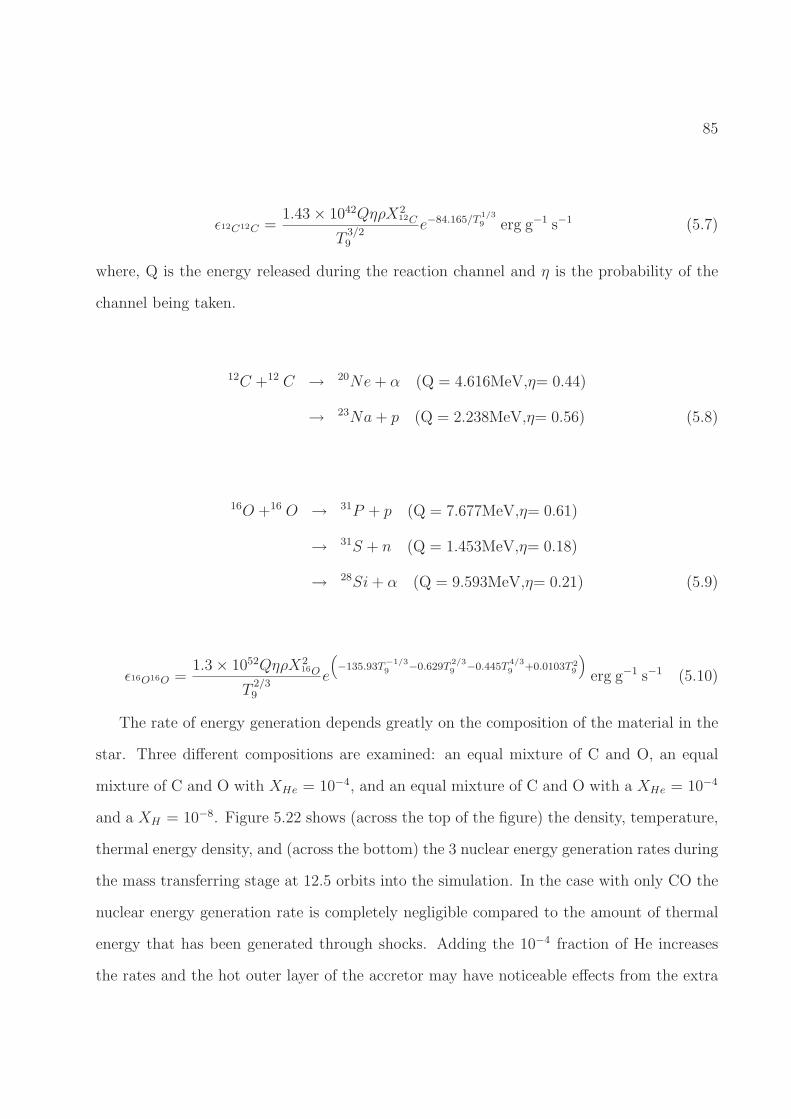
85

ǫ12C12C =1.43 × 1042QηρX2

12C

T3/29

e−84.165/T1/3

9 erg g−1 s−1 (5.7)

where, Q is the energy released during the reaction channel and η is the probability of the

channel being taken.

12C +12 C → 20Ne + α (Q = 4.616MeV,η= 0.44)

→ 23Na + p (Q = 2.238MeV,η= 0.56) (5.8)

16O +16 O → 31P + p (Q = 7.677MeV,η= 0.61)

→ 31S + n (Q = 1.453MeV,η= 0.18)

→ 28Si + α (Q = 9.593MeV,η= 0.21) (5.9)

ǫ16O16O =1.3 × 1052QηρX2

16O

T2/39

e

(

−135.93T−1/3

9−0.629T

2/3

9−0.445T

4/3

9+0.0103T 2

9

)

erg g−1 s−1 (5.10)

The rate of energy generation depends greatly on the composition of the material in the

star. Three different compositions are examined: an equal mixture of C and O, an equal

mixture of C and O with XHe = 10−4, and an equal mixture of C and O with a XHe = 10−4

and a XH = 10−8. Figure 5.22 shows (across the top of the figure) the density, temperature,

thermal energy density, and (across the bottom) the 3 nuclear energy generation rates during

the mass transferring stage at 12.5 orbits into the simulation. In the case with only CO the

nuclear energy generation rate is completely negligible compared to the amount of thermal

energy that has been generated through shocks. Adding the 10−4 fraction of He increases

the rates and the hot outer layer of the accretor may have noticeable effects from the extra

86

energy. If there is a small amount of H present, the nuclear energy generation would be

comparable to that from the shocks. Figure 5.23 plots the same quantities at 22 orbits into

the simulation, which is during the merger. At this time the CO burning would create an

amount of energy similar to the thermal energy from the shock, but only in a narrow region

at the surface of the accretor. The width of this region and its intensity expand if He and H

are added to the composition.

Despite the differences in initial conditions and included physics, the final objects for the

0.9 M⊙ and 0.6 M⊙ DWD mergers agree quite well with previously published results. The

accretor remains a cold core surrounded by a hot rapidly rotating thick disk and a cooler

outer disk.

87

Figure 5.6 Density contours in the equatorial plane for simulation Q2/3a, a DWD binarysystem constructed with the ZTWD equation of state and an initial mass ratio q=2/3.

88

0 1•109 2•109 3•109 4•109

distance from center (cm)

101102

103

104

105

106

107108

ρ (g

/cm

3 )

z - directionϖ - direction

Figure 5.7 Azimuthally averaged density in the equatorial plane plotted as a function ofdistance from the center of the merged object at a time of 12.59 minutes (20.83 orbits) forthe simulation Q2/3a, a DWD binary system constructed with the ZTWD equation of stateand an initial mass ratio q=2/3.

Figure 5.8 Meridional (,z) profile of the azimuthally averaged density at a time of 12.59minutes (20.83 orbits) for simulation Q2/3a, a DWD binary system constructed with theZTWD equation of state and an initial mass ratio q=2/3.

89

0 1•109 2•109 3•109 4•109

r (cm)

0.0

0.2

0.4

0.6

0.8

1.0

Ω/

Ωk

Figure 5.9 Angular velocity in the equatorial plane as a fraction of the Keplerian angularvelocity at a time of 12.59 minutes (20.83 orbits) for simulation Q2/3a, a DWD binarysystem constructed with the ZTWD equation of state and an initial mass ratio q=2/3. Alower ratio of Ω/ΩK indicates that the system is mainly supported by gas pressure and notrotation. A ratio of 1 indicates total rotational support.

90

Figure 5.10 Left: Density contours in the equatorial plane for the Q2/3b simulation of aq=2/3 DWD binary with a ZTWD plus ideal gas equation of state at three different times.Right: Temperature contours in the equatorial plane for the same Q2/3b simulation.

91

Figure 5.11 A continuation of Figure 5.10 Left: density contours in the equatorial plane forthe Q2/3b simulation at three different times. Left: Temperature contours in the equatorialplane for the same Q2/3b simulation.

92

Figure 5.12 Top: The mass of the accretor vs. time for a q=2/3 DWD binary with a totalmass of 1.5M⊙. Q2/3a has a ZTWD EOS and Q2/3b has a ZTWD plus ideal gas EOS.The mass is normalized to the initial mass and the time is displayed in orbital periods ofthe initial binary system. Middle: Mass of the donor normalized to the initial donor mass.Bottom: Mass ratio of the donor to accretor, q.

93

Figure 5.13 Top: The binary separation vs. time for a q=2/3 DWD binary with a totalmass of 1.5M⊙. Q2/3a has a ZTWD EOS and Q2/3b has a ZTWD plus ideal gas EOS. Theseparation is normalized to the initial separation and the time is displayed in orbital periodsof the initial binary system.

94

Figure 5.14 Top: The orbital angular momentum vs. time for a q=2/3 DWD binary with atotal mass of 1.5M⊙. Q2/3a has a ZTWD EOS and Q2/3b has a ZTWD plus ideal gas EOS.The orbital momentum is normalized to the initial total momentum and the time is displayedin orbital periods of the initial binary system. Middle: The spin angular momentum ofthe accretor normalized to the initial total angular momentum. Bottom: Spin angularmomentum of the donor normalized to the initial total angular momentum.

95

Figure 5.15 Top: The maximum density of the accretor vs. time for a q=2/3 DWD binarywith a total mass of 1.5M⊙. Q2/3a has a ZTWD EOS and Q2/3b has a ZTWD plus idealgas EOS. The density is normalized to the initial maximum density of the accretor. Bottom:The mass of a non-rotating ZTWD with a central density that corresponds to the maximumcentral density in the top panel as a function of time in orbital periods.

96

Figure 5.16 Top: The time rate of change of the mass of the accretor for a q=2/3 DWDbinary with a total mass of 1.5M⊙. Q2/3a has a ZTWD EOS and Q2/3b has a ZTWD plusideal gas EOS. The mass transfer rate is displayed in units of total mass of the binary perorbital period and time is displayed in initial orbital periods. Bottom: The negative of thetime rate of change of the mass of donor.

97

Figure 5.17 Meridional (,z) profile of the azimuthally averaged density at a time of 22.4orbits for simulation Q2/3b, a DWD binary system constructed with the ZTWD plus idealgas EOS and an initial mass ratio q=2/3.

98

0 1•109 2•109 3•109 4•109

r (cm)

0.0

0.2

0.4

0.6

0.8

1.0

Ω/

Ωk

Figure 5.18 Angular velocity in the equatorial plane as a fraction of the Keplerian angularvelocity at a time of 22.4 orbits for simulation Q2/3b, a DWD binary system constructedwith the ZTWD plus ideal gas equation of state and an initial mass ratio q=2/3. A lowerratio of Ω/ΩK indicates that the system is mainly supported by gas pressure and not rotation.A ratio of 1 indicates total rotational support.

99

0 1•109 2•109 3•109 4•109


101102

103

104

105

106

107108

ρ (g

/cm

3 )

z - directionϖ - direction

Figure 5.19 Azimuthally averaged density in the equatorial plane at a time of 22.40 orbits forsimulation Q2/3b, a DWD binary system constructed with the ZTWD plus ideal gas EOSand an initial mass ratio q=2/3.

100

0 1•109 2•109 3•109 4•109


106

107

108

109

T (

K)

z - direction

ϖ - direction

Figure 5.20 Azimuthally averaged temperature in the equatorial plane plotted as a functionof distance from the center of the accretor at a time of 22.40 orbits for simulation Q2/3b,a DWD binary system constructed with the ZTWD plus ideal gas EOS and an initial massratio q=2/3.

101

Figure 5.21 Each curve represents the maximum temperature at a give time for material witha density less than or equal to the corresponding density label in the legend. For examplethe red curve is the maximum value of the temperature in all cells with a density less thanor equal to 103 g/cm3 at the time on horizontal axis.

102

Figure 5.22 Contour plots in the equatorial plane for a q=2/3 DWD binary simulation,Q2/3b, with a total mass of 1.5M⊙ and a ZTWD plus ideal gas EOS at a time of 12.5 orbitalperiods (386s). Top Left: Mass density. Top Center: Temperature. Top Right: Energydensity of the ideal gas. Bottom Left: Power density from nuclear reactions assuming thesystem has an equal amount of C and O and no other elements, Bottom Center: Same as theleft panel except with XHe = 10−4 added. Bottom Right: Same as the center panel exceptwith XH = 10−8 added.

103

Figure 5.23 Same as Figure 5.22 except at an evolution time of 22.0 orbital periods (683s).

6. Conclusions

Based on the earlier work of Hachisu (1986a,b) and Hachisu, Eriguchi, & Nomoto (1986a)

we have developed a self-consistent-field technique that can be used to construct equilibrium

models of synchronously rotating DWD binaries having a range of total masses, mass ratios,

and binary separations. In addition to effects introduced by synchronous rotation, the dis-

torted structure of both stars in each converged model is governed by the zero-temperature

white dwarf equation of state (2.1) and a self-consistently determined, Newtonian gravita-

tional field. In an effort to illustrate the technique’s capabilities, we have constructed a set

of models along five sequences: Three sequences (‘A’, ‘B’, and ‘C’) mimic the last segment

of the detached “inspiral” phase of DWD binary evolutions during which both Mtot and q

are held constant as a decreases; and two sequences (‘D’ and ‘E’) mimic a semi-detached

“conservative mass transfer” phase of evolution during which Mtot is held fixed and the less

massive star stays in marginal contact with its Roche lobe, but q steadily decreases while a

steadily increases.

Along each inspiral sequence, the functional dependence of Jtot and Etot on the orbital

separation can be well understood in terms of simple analytical expressions that describe

two spinning spherical white dwarfs in circular orbit about one another. For a given total

mass and separation, the calculated orbital frequencies along each inspiral sequence deviate

measurably from associated Keplerian frequencies only in models for which the Roche-lobe

filling factor of the less-massive star is ∼> 60%. But, at least for the sequences examined

here, the deviation from Keplerian frequencies is never more than 1% even at contact.

Along both conservative mass-transfer sequences, we have documented how a, Ω, Jtot and

Etot vary with the system mass ratio as q decreases by roughly a factor of two, from q = 1.0

down to q ∼< 0.5. Along each sequence we have compared our numerically determined values

104

105

of a at various values of q with the analytic a(q) function (3.12) that is derived by setting the

radius of the less massive star, as specified by the Nauenberg (1972) mass-radius relation,

equal to the Roche-lobe radius, as approximated by Eggleton (1983). Qualitatively, our

results show the same a(q) behavior that is predicted by this analytic expression. However,

at a given q the value of a derived from our models is consistently ∼ 8% larger than the value

obtained from Eq. (3.12). The analytic expression could be brought into closer quantitative

agreement with our numerical results if the leading coefficient in Eq. (3.12) is increased by

8%, that is, if the expression’s leading coefficient is changed from 0.0229 to 0.0247. This

modification will, in turn, decrease the Keplerian frequency obtained from the analytic a(q)

expression by ∼ 9%, simultaneously bringing the analytically predicted orbital frequency

into much closer agreement with our numerically determined values of Ω. Along both of our

conservative mass-transfer sequences, the plot of Jtot(q) displays an extremum at a value of

q ∼< 2/3. The location of this extremum is almost certainly identifying the value of qcrit that

is relevant along both sequences.

We have demonstrated that both an n=3/2 polytropic binary with a mass ratio of q=0.7

and a DWD binary with a total mass of 1.5 M⊙ and a mass ratio of q=2/3 are dynamically

unstable after the onset of mass transfer. In both the polytropic and DWD binaries the

onset of mass transfer led to the eventual tidal disruption of the donor with most of the

donor material forming a disk around the accretor, which has remained mostly intact.

In the simulation with the ZTWD plus ideal gas EOS, Q2/3b, we find that mass transfer

can occur for many orbits before the eventual tidal disruption. During this phase of steady

mass transfer the outer layers of the accretor are heated to ∼ 108K. However, this heating

does not penetrate into the higher density regions of the accretor and the interior remains

between ∼ 105-107K. If a composition of pure C and O is assumed, there should not be sig-

nificant energy generation from nuclear fusion during the mass transfer phase. The addition

106

of small amounts of He and H can increase the expected levels of nuclear fusion, but only in

the hot outer layer of the accretor.

The final merged structure from the Q2/3b simulation is a cold (< 3 × 107K) core of

accretor material that is pressure supported. Around this core is a hot (∼ 5×108K) envelope

of material that is also primarily pressure supported. This pressure supported inner object

lies at the center of a disk with a thickness slightly larger than the diameter of the core

and with a radius that is approximately 6 times greater than that of the core. This disk

is primarily supported by rotation and has a temperature of 107K-108K. The temperatures

and densities in the hottest region are favorable for the fusion of C and O, but in a very

small region and not at a rate high enough to lead to an explosive event. Therefore, for the

total mass and mass ratio examined in this simulation it is unlikely that a supernova would

occur during or immediately following the merger. This does not rule out DWD mergers

as progenitors to Type Ia supernovae. Viscous effects within the disk will cause the disk

material to accrete onto the core over a longer period of time. If the time scale for accretion

of the disk is shorter than the time scale for significant cooling of the gas then density and

temperatures could reach values that would result in a delayed supernova.

Bibliography

Balay, S., Buschelman, K., Eijkhout, V., Gropp, W., Kaushik, D., Knepley, M., McInnes,L., Smith, B., and Zhang, H. 2004, PETSc Users Manual, ANL-95/11 - Revision 2.1.5

Benz, W., Cameron, A. G. W., Press, W. H., & Bowers, R.L. 1990, ApJ, 348,647

Chandrasekhar, S. 1935, MNRAS, 95, 207

Chandrasekhar, S. 1967, An Introduction to the Study of Stellar Structure, New York: Dover

Cohl, H. and Tohline, J. 1999, ApJ, 527, 86

Cox, A. N. 2000, Allen’s Astrophysical Quantities, 4th edition, New York: Springer-Verlag

D’Souza, M. C. R., Motl, P. M., Tohline, J. E., & Frank, J. 2006, ApJ, 643, 381

Eggleton, P. P. 1983, ApJ, 268, 368

Even, W., & Tohline, J. E. 2009, ApJS, 184, 248

Guerrero, J., Garcia-Berro, E., & Isern, J. 2004, A&A, 413, 257

Hachisu, I. 1986a, ApJS, 61, 479

Hachisu, I. 1986b, ApJS, 62, 461

Hachisu, I., Eriguchi, Y., & Nomoto, K. 1986a, ApJ, 308, 161

Hachisu, I., Eriguchi, Y., & Nomoto, K. 1986b, ApJ, 311, 214

Livio, M. 2000, in Type Ia Supernovae: Theory and Cosmology, ed. J. C. Niemeyer, & J. W.Truran (Cambridge Univ. Press), 33

Marsh, T. R., Nelemans, G., & Steeghs, D. 2004, MNRAS, 350, 113

Motl, M. P., 2001, Dissertation, Louisiana State University

Motl, M. P., Tohline, J. E., Frank, J., 2002, ApJS, 138, 121

Motl, M. P., Frank, J., Tohline, J. E., & D’Souza, M. C. R. 2007, ApJ, 670, 1314

Nauenberg, M. 1972, ApJ, 175, 417

Nelemans, G., Portegies Zwart, S.F., Verbunt, F., & Yungleson, L. R. 2001, A&A, 368, 939

New, C. B. Kimberly, and Tohline, Joel E. 1997, ApJ, 490, 311

Ostriker, J.P., and Mark, J W-K. 1964, ApJ, 151, 1075

107

108

Padmanabhan, T., 2000 ,Theoretical Astrophysics Volume I: Astrophysical Processes, Cam-bridge University Press

Ramsay, G., Brocksopp, C., Groot, P. J., Hakala, P., Lehto, H., Marsh, T. R., Napiwotzki,R., Nelemans, G., Potter, S., Slee, B., Steeghs, D., & Wu, K. 2007, ASP Conference Series,15th European Workshop on White Dwarfs, 372, 425 (arXiv:astro-ph/0610357v1)

Rucinski, S. M. 1988, AJ, 95, 1895

Segretain, L., Chabrier, G., & Mochkovitch, R. 1997, ApJ, 481, 355

Verbunt, F., & Rappaport, S. 1988, ApJ, 332, 193

Yoon, S.-C., Podsiadlowski, Ph., & Rosswog, S. 2007, MNRAS, 380, 933

Zapolsky, H. S., & Salpeter, E. E. 1969, ApJ, 158, 809

Appendix A: White Dwarf Mass-RadiusRelationship

A.0.1 The Chandrasekhar Mass

Chandrasekhar (1935) was the first to construct models of spherically symmetric stars using

the equation of state defined by Eq. (2.1) and, in so doing, demonstrated that the maximum

mass of an isolated, nonrotating white dwarf is Mch = 1.44(µe/2)M⊙, where µe is the number

of nucleons per electron and, hence, depends on the chemical composition of the WD. A

concise derivation of Mch (although, at the time, it was referred to as M3) is presented in

Chapter XI of Chandrasekhar (1967), where we also find that the expressions for the two

key coefficients in Eqs. (2.1) and (2.2) are,

A ≡πm4

ec5

3h3, (A.1)

Bµ−1e ≡

8πmp

3

(

mec

h

)3

. (A.2)

Numerical values for A and Bµ−1e are given here in Table B.1 along with values of the physical

constants c, h, me, and mp that we have used (column 2) and that Chandrasekhar (1967)

used (column 3) to determine the values of A and Bµ−1e . The derived analytic expression

for the limiting mass is,

µ2eMch = 4πm3

(

2A

πG

)3/2 µ2e

B2= 1.14205 × 1034 g , (A.3)

where the coefficient,

m3 ≡(

−ξ2dθ3

dξ

)

ξ=ξ1(θ3)= 2.01824 , (A.4)

represents a structural property of n = 3 polytropes (γ = 4/3 gases) whose numerical

value can be found in Chapter IV , Table 4 or Chandrasekhar (1967). We note as well that

109

110

Chandrasekhar (1967) identified a characteristic radius, ℓ1, for WDs given by the expression,

ℓ1µe ≡(

2A

πG

)1/2 µe

B= 7.71395 × 108 cm . (A.5)

A.0.2 The “Nauenberg” Mass-Radius Relationship

Nauenberg (1972) derived an analytic approximation for the mass-radius relationship exhib-

ited by isolated, spherical WDs that obey the ZTWD equation of state given in Eq. (2.1).

Specifically, he offered an expression of the form,

R = R0

[

(1 − n4/3)1/2

n1/3

]

, (A.6)

where,

n ≡M

(µmµ)N0

, (A.7)

N0 ≡(3π2ζ)1/2

ν3/2

[

hc

2πG(µmµ)2

]3/2

=µ2

em2p

(µmµ)3

[

4πζ

m23ν

3

]1/2

Mch , (A.8)

R0 ≡ (3π2ζ)1/3[

h

2πmec

]

N1/30 =

(µemp)

(µmµ)

[

4πζ

ν

]1/2

ℓ1 , (A.9)

mµ is the atomic mass unit (see Table B.1), µ is the mean molecular weight of the gas, and ζ

and ν are two adjustable parameters in Nauenberg’s analytic approximation, both of which

are expected to be of order unity. By assuming that the average particle mass denoted

by Chandrasekhar (1967) as (µemp) is identical to the average particle mass specified by

Nauenberg (1972) as (µmµ) and, following Nauenberg’s lead, by setting ν = 1 and∗,

ζ =m2

3

4π= 0.324142 , (A.10)

in Eq. (A.8) we see that,

(µmµ)N0 = Mch . (A.11)

∗Actually, Nauenberg (1972) sets ζ = 0.323.

111

Hence, the denominator in (A.7) becomes the Chandrasekhar mass. Furthermore, expres-

sions (A.9) and (A.6) become, respectively,

µeR0 = m3(ℓ1µe) = 1.55686 × 109 cm , (A.12)

and,

R = R0

[1 − (M/Mch)4/3]1/2

(M/Mch)1/3

. (A.13)

Finally, by adopting the values of M⊙ and R⊙ listed in Table B.1, we obtain essentially† the

identical approximate, analytic mass-radius relationship for ZTWDs presented in Eqs. (27)

and (28) of Nauenberg (1972):

R

R⊙

=0.0224

µe

[1 − (M/Mch)4/3]1/2

(M/Mch)1/3

, (A.14)

where,

Mch

M⊙

=5.742

µ2e

. (A.15)

A.0.3 The “Eggleton” Mass-Radius Relationship

Verbunt & Rappaport (1988) introduced the following approximate, analytic expression for

the mass-radius relationship of a “completely degenerate . . . star composed of pure helium”

(i.e., µe = 2), attributing its origin to Eggleton (private communication):

R

R⊙

= 0.0114[(

M

Mch

)−2/3

−(

M

Mch

)2/3]1/2[

1 + 3.5(

M

Mp

)−2/3

+(

M

Mp

)−1]−2/3

,(A.16)

where Mp is a constant whose numerical value is 0.00057M⊙. This “Eggleton” mass-radius re-

lationship has been used widely by researchers when modeling the evolution of semi-detached

†The numerical coefficients that appear here in Eqs. (A.14) and (A.15) differ slightly from the onespresented in Eqs. (27) and (28), respectively, of Nauenberg (1972) presumably because the values of thephysical constants — such as M⊙ and R⊙ — that we have adopted in this paper (see Table B.1) are slightlydifferent from the values adopted by Nauenberg.

112

binary star systems in which the donor is a ZTWD. Since the Nauenberg (1972) mass-radius

relationship (A.14) is retrieved from Eq. (A.16) in the limit M/Mp ≫ 1, it seems clear that

Eggleton’s contribution was the insertion of the term in square brackets involving the ratio

M/Mp which, as Marsh et al. (2004) phrase it, “allows for the change to a constant density

configuration at low masses (Zapolsky & Salpeter, 1969).” Here we have only constructed

binary star systems in which the internal structure of both stars is governed by the ZTWD

equation of state (2.1). Hence it is appropriate for us to compare the properties of our mod-

eled systems to behaviors predicted by the “Nauenberg,” not the “Eggleton,” mass-radius

relationship.

Appendix B: Physical Constants

113

114

Table B.1. Physical Constants

Constantsa This Paperb Chandrasekhar (1967)c

(1) (2) (3)

c (cm s−1) 2.99792 × 10+10 2.9978 × 1010

h (erg · s) 6.62608 × 10−27 6.62 × 10−27

me (g) 9.10939 × 10−28 9.105 × 10−28

mp (g) 1.67262 × 10−24 1.672 × 10−24

mµ (g) 1.66054 × 10−24 · · ·G (cm3 g−1 s−2) 6.6726 × 10−8 6.62 × 10−8

M⊙ (g) 1.9891 × 1033 1.985 × 1033

R⊙ (cm) 6.955 × 1010 6.951 × 1010

A (dynes cm−2) 6.00228 × 1022 6.01 × 1022

Bµ−1e (g cm−3) 9.81011 × 105 9.82 × 105

ℓ1µe (cm) 7.71395 × 108 7.705 × 108

aSpeed of light, c; Planck’s constant, h; mass of the electron,me; mass of the proton mp; atomic mass unit, mµ; universalgravitational constant, G; solar mass, M⊙; solar radius, R⊙;as used in the ZTWD equation of state (2.1), A = πm4

ec5/3h3

and Bµ−1e = 8πm3

ec3mp/3h

3; the characteristic WD lengthscale, ℓ1µe = (2A/πG)1/2(µe/B).

bDrawn from Cox (2000).

cDrawn from Appendix I, Table 32 of Chandrasekhar(1967).

Appendix C: List of Variables

115

116

Table C.1. List of Variables

Variable Definition

Am Angular momentum densitya Separation of binaryacrit Separation of binary at which one star overfills its Roche lobeC Bernoulli constantcp Specific heatcs Speed of soundE Energy DensityEb Binding energy of a starEdeg Energy density from electron degeneracyEK Kinetic energy densityEorb Kinetic energy of 2 point mass stars in a circular orbitEpm Binding plus kinetic energy for 2 point mass stars in a circular orbitEtot Total energyF Negative of the effective potentialfRL Ratio of the volume of a star to its Roche lobe volumeH Enthalpy per unit massI Moment of inertiaJpm Angular momentum of 2 point masses in a circular orbitJss Angular momentum of 2 synchronously rotating spheres in a circular orbitJspin Angular momentum in the rotation of the starJtot Total angular momentumK Kinetic energyk Radius of gyrationℓ Ratio of the radius of the donor to binary seperationM1 Mass of the accretorM2 Mass of the donorMch Chandrasekhar mass limitMtot Total mass of the systemM⊙ Solar Massn Polytopic indexNz Number of grid cells in the vertical dimensionNθ Number of grid cells in the azimuthal dimensionN Number of grid cells in the radial dimensionP PressurePdeg Degeneracy pressurePgas Ideal gas pressureQ Effective energy released in a nuclear reactionq Ratio of donor mass to accretor massR RadiusR1 Radius of the accretor

117

Table C.1. - Continued

Variable Definition

R2 Radius of the donorR⊙ Solar radiusr Spherical radial coordinate~r Position vector~r1 Position vector from the center of mass of the accretor~r2 Position vector from the center of mass of the donorℜ Gas ConstantSm Radial momentum densityT TemperatureTm Vertical momentum densityt TimeU Internal energyV VolumeVE Virial error~v VelocityW Gravitational potential energy

x Dimensionless parameter,(

ρB

)1/3

X Mass fraction of an elementXm Mass fraction of elements heavier than heliumZ Cylindrical vertical coordinateγ Ratio of specific heatsǫ Nuclear energy generation rateη Fractional probability of a given channel in a nuclear reactionθ Cylindrical azimuthal coordinateκ Polytropic constantµ Mean molecular weightµe Ratio of nucleons to electronsΠ Globally averaged pressureρ Mass densityρp Density cut-off for calculating the ideal gas pressureρ∗ Maximum density of the donorτ Entropy TracerΦ Gravitational potentialΦeff Effective potential in the rotating frameΦR Roche potentialΩ Binary orbital frequencyΩk Kepler frequency Cylindrical radial coordinate∗ Distance from the outer edge of the donor to the center of mass of the system

Appendix D: Letter of Permission

Before your article can be published in an American Astronomical Society (AAS) jour-

nal, we require you to grant and assign the entire copyright in it to the AAS. The copyright

consists of all rights protected by the copyright laws of the United States and of all foreign

countries, in all languages and forms of communication, including the right to furnish the

article or the abstracts to abstracting and indexing services, and the right to republish the

entire article in any format or medium. In return, the AAS grants to you the non-exclusive

right of republication, subject only to your giving appropriate credit to the journal in which

your article is published. This non-exclusive right of republication includes your right to

allow reproduction of parts of your article wherever you wish, and permits you to post the

published (PDF) version of your article on your personal web site.

(http://www.iop.org/EJ/journal/-page=extra.3/APJ)

118

Vita

Wesley Paul Even was born in Gilbertville, Iowa, on September 2, 1980. He earned his

bachelor’s degree in physics in 2003 from the University of Northern Iowa. In August of

2003, he enrolled at Louisiana State University. He received his master’s degree in 2008, and

expects to receive his doctoral degree in May 2010.

119

Mass transfer and mergers in double white dwarf binaries

Documents

Transcript of Mass transfer and mergers in double white dwarf binaries