Universität Potsdam Institut für Informatik

Lehrstuhl Maschinelles Lernen

Recommendation

Tobias Scheffer

Inte

lligent D

ata

Analy

sis

II

Recommendation Engines

Recommendation of products, music, contacts, ..

Based on user features, item features, and past

transactions: sales, reviews, clicks, …

User-specific recommendations, no global ranking

of items.

Feedback loop: choice of recommendations

influences available transaction and click data.

2

Inte

lligent D

ata

Analy

sis

II

Netflix Prize

Data analysis challenge, 2006-2009

Netflix made rating data available: 500,000 users,

18,000 movies, 100 million ratings

Challenge: predict ratings that were held back for

evaluation; improve by 10% over Netflix‘s

recommendation

Award: $ 1 million.

3

Inte

lligent D

ata

Analy

sis

II

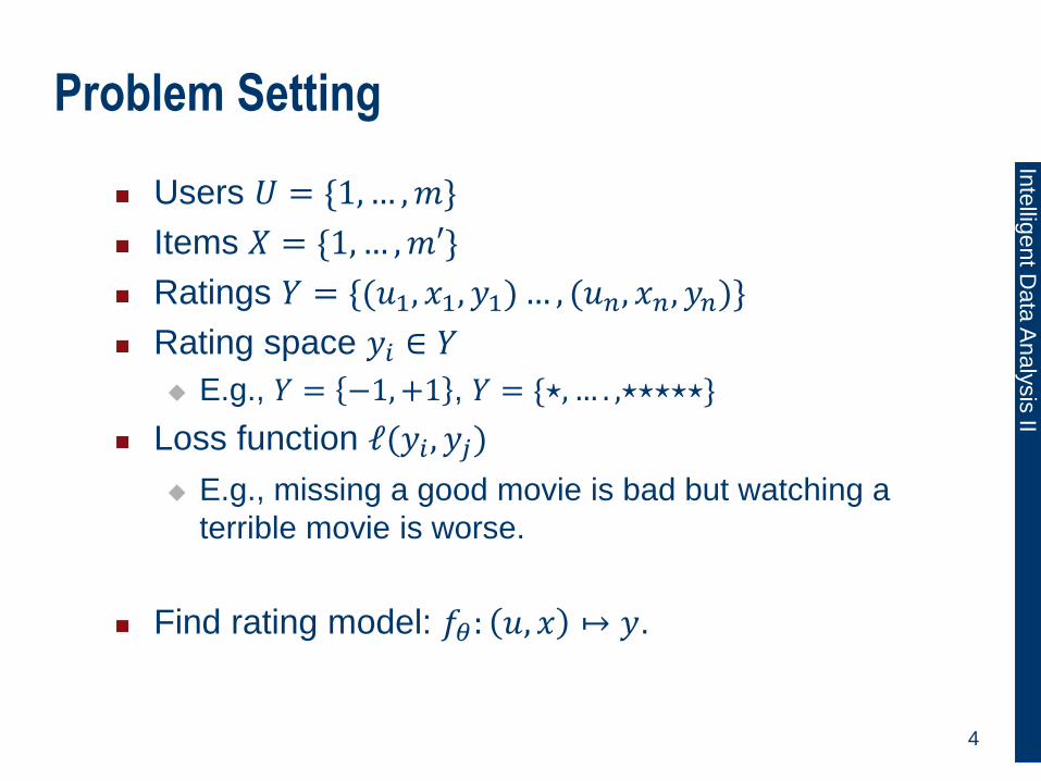
Problem Setting

Users 𝑈 = {1,… ,𝑚}

Items 𝑋 = {1,… ,𝑚′}

Ratings 𝑌 = {(𝑢1, 𝑥1, 𝑦1)… , (𝑢𝑛, 𝑥𝑛, 𝑦𝑛)}

Rating space 𝑦𝑖 ∈ 𝑌

E.g., 𝑌 = −1,+1 , 𝑌 = {⋆,… . ,⋆⋆⋆⋆⋆}

Loss function ℓ(𝑦𝑖 , 𝑦𝑗)

E.g., missing a good movie is bad but watching a

terrible movie is worse.

Find rating model: 𝑓𝜃: 𝑢, 𝑥 ↦ 𝑦.

4

Inte

lligent D

ata

Analy

sis

II

Problem Setting: Matrix Notation

Users 𝑈 = {1,… ,𝑚}

Items 𝑋 = {1,… ,𝑚′}

Ratings 𝑌 =

𝑦11 𝑦12

𝑦21 𝑦23

𝑦33

Rating space 𝑦𝑖 ∈ Υ

E.g.,Υ = −1,+1 ,Υ = {⋆,… . ,⋆⋆⋆⋆⋆}

Loss function ℓ(𝑦𝑖 , 𝑦𝑗)

5

item 1 2 3

user 1 user 2 user 3

Incomplete matrix

Inte

lligent D

ata

Analy

sis

II

Problem Setting

Model 𝑓𝜃(𝑢, 𝑥)

Find model parameters that minimize risk

𝜃∗ = argminθ∫ ∫ ∫ ℓ 𝑦, 𝑓𝜃 𝑢, 𝑥 𝑝 𝑢, 𝑥, 𝑦 𝑑𝑥𝑑𝑢𝑑𝑟

As usual: 𝑝 𝑢, 𝑥, 𝑦 is unknown → minimize

regularized empirical risk

𝜃∗ = argminθ ℓ 𝑦𝑖 , 𝑓𝜃 𝑢𝑖 , 𝑥𝑖

𝑛

𝑖=1+ 𝜆Ω(𝜃)

6

Inte

lligent D

ata

Analy

sis

II

Content-Based Recommendation

Idea: User may like movies that are similar to other

movies which they like.

Requirement: attributes of items, e.g.,

Tags,

Genre,

Actors,

Director,

…

7

Inte

lligent D

ata

Analy

sis

II

Content-Based Recommendation

Feature space for items

E.g., Φ = comedy, action, year, dir tarantino, dir cameron T

𝜙 avatar = 0, 1, 2009, 0, 1 T

8

Inte

lligent D

ata

Analy

sis

II

Content-Based Recommendation

Users 𝑈 = {1,… ,𝑚}

Items 𝑋 = {1,… ,𝑚′}

Ratings 𝑌 = {(𝑢1, 𝑥1, 𝑦1)… , (𝑢𝑛, 𝑥𝑛, 𝑦𝑛)}

Rating space 𝑦𝑖 ∈ 𝑌

E.g.,Υ = −1,+1 ,Υ = {⋆,… . ,⋆⋆⋆⋆⋆}

Loss function ℓ(𝑦𝑖 , 𝑦𝑗)

E.g., missing a good movie is bad but watching a

terrible movie is worse.

Feature function for items: 𝜙: 𝑥 ↦ ℝ𝑑

Find rating model: 𝑓𝜃: 𝑢, 𝑥 ↦ 𝑦.

9

Inte

lligent D

ata

Analy

sis

II

Independent Learning Problems for Users

Minimize regularized empirical risk

𝜃∗ = argminθ ℓ 𝑦𝑖 , 𝑓𝜃 𝑢𝑖 , 𝑥𝑖

𝑛

𝑖=1+ 𝜆Ω(𝜃)

One model per user:

𝑓𝜃𝑢𝑥 ↦ Υ

One learning problem per user:

𝜃𝑢∗ = argmin𝜃𝑢

ℓ 𝑦𝑖 , 𝑓𝜃𝑢𝑥𝑖

𝑖:𝑢𝑖=𝑢+ 𝜆Ω(𝜃𝑢)

10

Inte

lligent D

ata

Analy

sis

II

Independent Learning Problems for Users

One learning problem per user:

∀𝑢: 𝜃𝑢∗ = argmin𝜃𝑢

ℓ 𝑦𝑖 , 𝑓𝜃𝑢𝑥𝑖

𝑖:𝑢𝑖=𝑢+ 𝜆Ω(𝜃𝑢)

Use any model class and learning mechanism; e.g.,

𝑓𝜃𝑢𝑥𝑖 = 𝜙 𝑥𝑖

T𝜃𝑢

Logistic loss + ℓ2 regularization: logistic regression

Hinge loss + ℓ2 regularization: SVM

Squared loss + ℓ2 regularization: ridge regression

11

Inte

lligent D

ata

Analy

sis

II

Independent Learning Problems for Users

Obvious disadvantages of independent problems:

Commonalities of users are not exploited,

User does not benefit from ratings given by other

users,

Poor recommendations for users who gave few

ratings.

Rather use joint prediction model:

Recommendations for each user should benefit from

other osers’ ratings.

12

Inte

lligent D

ata

Analy

sis

II

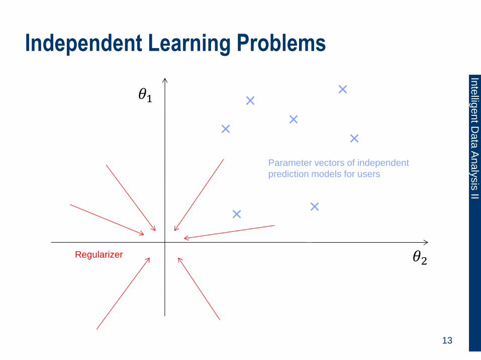
Independent Learning Problems

13

Parameter vectors of independent

prediction models for users

Regularizer

𝜃1

𝜃2

Inte

lligent D

ata

Analy

sis

II

Joint Learning Problem

14

Parameter vectors of independent

prediction models for users

Regularizer

𝜃1

𝜃2

Inte

lligent D

ata

Analy

sis

II

Joint Learning Problem

Standard ℓ2 regularization follows from the

assumption that model parameters are governed by

normal distribution with mean vector zero.

Instead assume that there is a non-zero population

mean vector.

15

Inte

lligent D

ata

Analy

sis

II

Joint Learning Problem

16

0

Graphical model of

hierarchical prior

𝜃1 𝜃2 𝜃𝑚

𝜃

Σ

Inte

lligent D

ata

Analy

sis

II

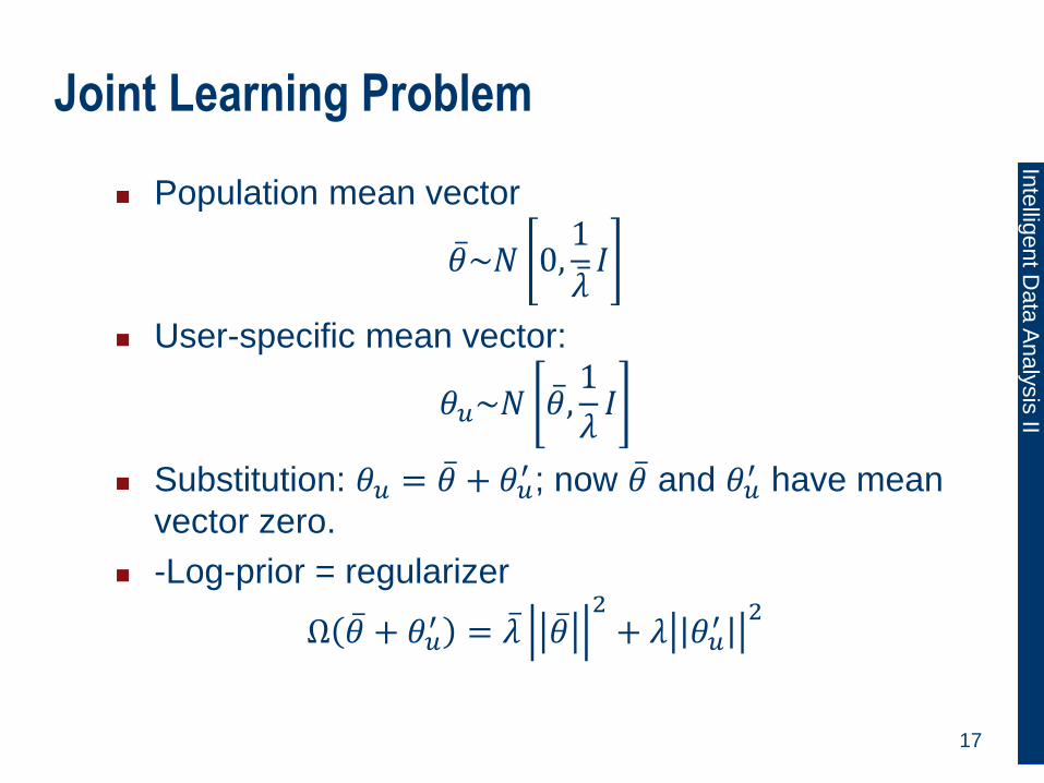
Joint Learning Problem

Population mean vector

𝜃 ~𝑁 0,1

𝜆 𝐼

User-specific mean vector:

𝜃𝑢~𝑁 𝜃 ,1

𝜆𝐼

Substitution: 𝜃𝑢 = 𝜃 + 𝜃𝑢′ ; now 𝜃 and 𝜃𝑢

′ have mean

vector zero.

-Log-prior = regularizer

Ω 𝜃 + 𝜃𝑢′ = 𝜆 𝜃

2+ 𝜆 𝜃𝑢

′ 2

17

Inte

lligent D

ata

Analy

sis

II

Joint Learning Problem

Joint optimization problem:

min𝜃1′ ,…,𝜃𝑚

′ ,𝜃 ℓ 𝑦𝑖 , 𝑓𝜃𝑢

′ +𝜃 𝑥𝑖 + 𝜆Ω 𝜃′𝑢 + 𝜆 Ω(𝜃 )

𝑖:𝑢𝑖=𝑢𝑢

Parameters 𝜃𝑢′ are independent, 𝜃 is shared.

Hence, 𝜃𝑢 are coupled.

18

𝜃𝑢 = 𝜃 + 𝜃𝑢′

Coupling

strength

Global

regularization

Inte

lligent D

ata

Analy

sis

II

Discussion

Each user benefits from other users‘ ratings.

Does not take into account that users have different

tastes.

Two sci-fi fans may have similar preferences, but a

horror-movie fan and a romantic-comedy fan do

not.

Idea: look at ratings to determine how similar users

are.

19

Inte

lligent D

ata

Analy

sis

II

Collaborative Filtering

Idea: People like items that are liked by people who

have similar preferences.

People who give similar ratings to items probably

have similar preferences.

This is independent of item features.

20

Inte

lligent D

ata

Analy

sis

II

Collaborative Filtering

Users 𝑈 = {1,… ,𝑚}

Items 𝑋 = {1,… ,𝑚′}

Ratings 𝑌 = {(𝑢1, 𝑥1, 𝑦1)… , (𝑢𝑛, 𝑥𝑛, 𝑦𝑛)}

Rating space 𝑦𝑖 ∈ Υ

E.g.,Υ = −1,+1 ,Υ = {⋆,… . ,⋆⋆⋆⋆⋆}

Loss function ℓ(𝑦𝑖 , 𝑦𝑗)

Find rating model: 𝑓𝜃: 𝑢, 𝑥 ↦ 𝑦.

21

Inte

lligent D

ata

Analy

sis

II

Collaborative Filtering by Nearest Neighbor

Define distance function on users:

𝑑(𝑢, 𝑢′)

Predicted rating:

𝑓𝜃 𝑢, 𝑥 = 1

𝑘𝑦𝑢𝑖,𝑥

𝑘 nearestneighbors 𝑢𝑖 of 𝑢

Predicted rating is the average rating of the

𝑘 nearest neighbors in terms of 𝑑 𝑢, 𝑢′ .

No learning involved.

Performance hinges on 𝑑(𝑢, 𝑢′).

22

Inte

lligent D

ata

Analy

sis

II

Collaborative Filtering by Nearest Neighbor

Define distance function on users:

𝑑 𝑢, 𝑢′ =1

𝑚′ 𝑦𝑢′,𝑥 , −𝑦𝑢,𝑥

2𝑚′

𝑥=1

Euclidean distance between ratings for all items.

Skip items that have not been rated by both users.

23

Inte

lligent D

ata

Analy

sis

II

Extensions

Normalize ratings (subtract mean rating of user,

divide by user‘s standard deviation)

Weight influence of neighbors by inverse of

distance.

Weight influence of neighbors with number of jointly

rated items.

𝑓𝜃 𝑢, 𝑥 =

1

𝑑(𝑢, 𝑢𝑖)𝑦𝑢𝑖,𝑥𝑘 nearest

neighbors 𝑢𝑖 of 𝑢

1

𝑑(𝑢, 𝑢𝑖)𝑘 nearestneighbors 𝑢𝑖 of 𝑢

24

Inte

lligent D

ata

Analy

sis

II

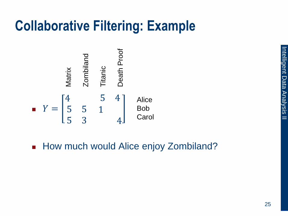
Collaborative Filtering: Example

𝑌 =4 5 45 5 15 3 4

How much would Alice enjoy Zombiland?

25

Matr

ix

Zom

bila

nd

Titanic

Death

Pro

of

Alice

Bob

Carol

Inte

lligent D

ata

Analy

sis

II

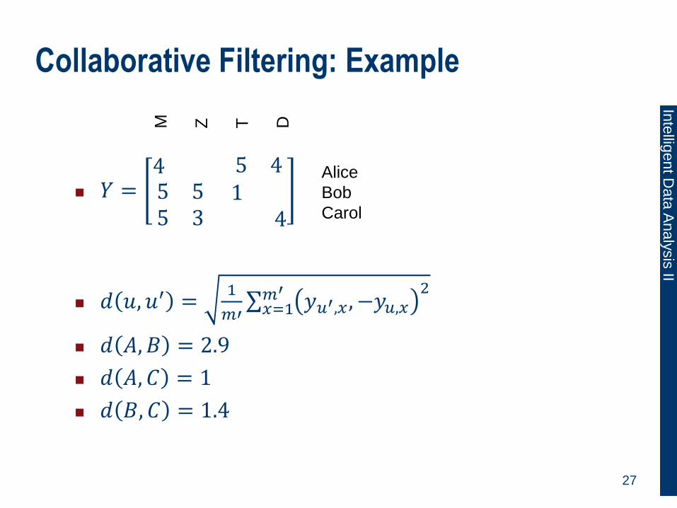
Collaborative Filtering: Example

𝑌 =4 5 45 5 15 3 4

𝑑 𝑢, 𝑢′ =1

𝑚′ 𝑦𝑢′,𝑥 , −𝑦𝑢,𝑥

2𝑚′

𝑥=1

𝑑 𝐴, 𝐵 =

𝑑 𝐴, 𝐶 =

𝑑 𝐵, 𝐶 =

26

M

Z

T

D

Alice

Bob

Carol

Inte

lligent D

ata

Analy

sis

II

Collaborative Filtering: Example

𝑌 =4 5 45 5 15 3 4

𝑑 𝑢, 𝑢′ =1

𝑚′ 𝑦𝑢′,𝑥 , −𝑦𝑢,𝑥

2𝑚′

𝑥=1

𝑑 𝐴, 𝐵 = 2.9

𝑑 𝐴, 𝐶 = 1

𝑑 𝐵, 𝐶 = 1.4

27

M

Z

T

D

Alice

Bob

Carol

Inte

lligent D

ata

Analy

sis

II

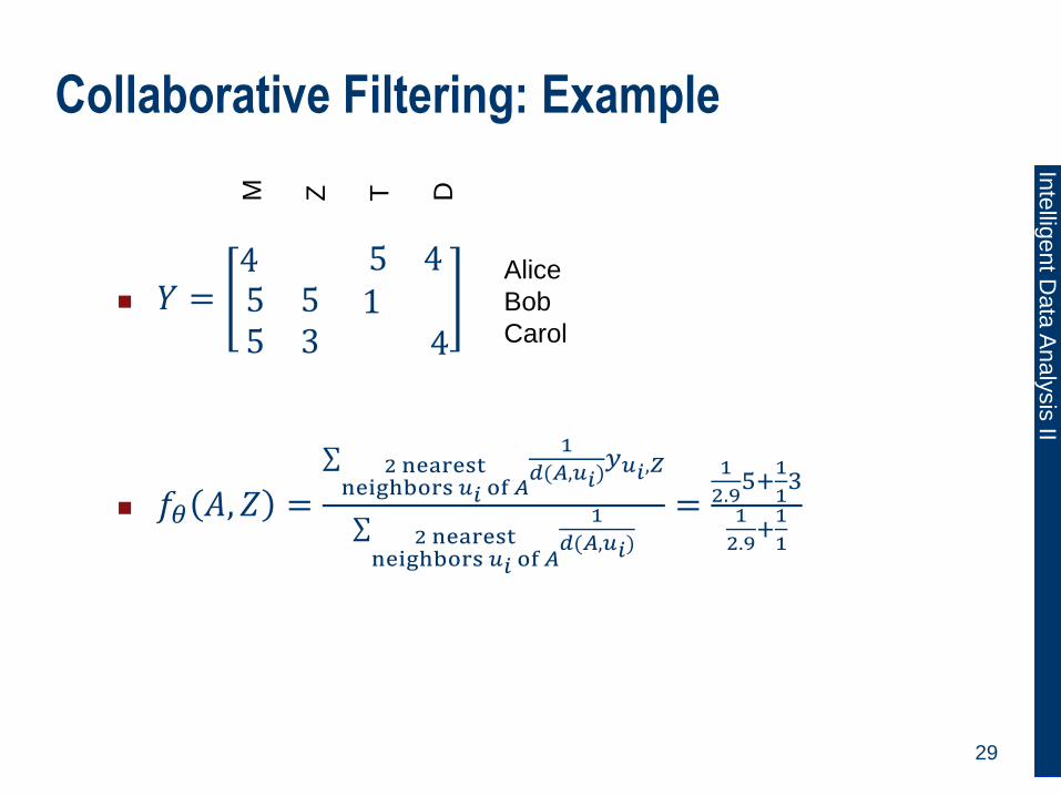
Collaborative Filtering: Example

𝑌 =4 5 45 5 15 3 4

𝑓𝜃 𝐴, 𝑍 =

1

𝑑(𝐴,𝑢𝑖)𝑦𝑢𝑖,𝑍2 nearest

neighbors 𝑢𝑖 of 𝐴

1

𝑑(𝐴,𝑢𝑖)2 nearest

neighbors 𝑢𝑖 of 𝐴

=

28

M

Z

T

D

Alice

Bob

Carol

Inte

lligent D

ata

Analy

sis

II

Collaborative Filtering: Example

𝑌 =4 5 45 5 15 3 4

𝑓𝜃 𝐴, 𝑍 =

1

𝑑(𝐴,𝑢𝑖)𝑦𝑢𝑖,𝑍2 nearest

neighbors 𝑢𝑖 of 𝐴

1

𝑑(𝐴,𝑢𝑖)2 nearest

neighbors 𝑢𝑖 of 𝐴

=1

2.95+

1

13

1

2.9+

1

1

29

M

Z

T

D

Alice

Bob

Carol

Inte

lligent D

ata

Analy

sis

II

Collaborative Filtering: Discussion

K nearest neigbor and similar methods are called

memory-based approaches.

There are no model parameters, no optimization

criterion is being optimized.

Each prediction reuqires an iteration over all training

instances → impractical!

Better to train a model by minimizing an appropriate

loss function over a space of model parameter, then

use model to make predictions quickly.

30

Inte

lligent D

ata

Analy

sis

II

Latent Features

Idea: Instead of ad-hoc definition of distance

between users, learn features that actually

represent preferences.

If, for every user 𝑢, we had a feature vector 𝜓𝑢 that

describes their preferences,

Then we could learn parameters 𝜃𝑥 for item 𝑥 such

that 𝜃𝑥T𝜓𝑢 quantifies how much 𝑢 enjoys 𝑥.

31

Inte

lligent D

ata

Analy

sis

II

Latent Features

Or, turned around,

If, for every item 𝑥 we had a feature vector 𝜙𝑥 that

characterizes its properties,

We could learn parameters 𝜃𝑢 such that 𝜃𝑢T𝜙𝑥

quantifies how much 𝑢 enjoys 𝑥.

In practice some user attributes 𝜓𝑢 and item

attributes 𝜙𝑥 are usually available, but they are

insufficient to understand 𝑢‘s preferences and 𝑥‘s

relevant properties.

32

Inte

lligent D

ata

Analy

sis

II

Latent Features

Idea: construct user attributes 𝜓𝑢 and item

attributes 𝜙𝑥 such that ratings in training data can

be predicted accurately.

Decision function: 𝑓Ψ,Φ 𝑢, 𝑥 = 𝜓𝑢

T𝜙𝑥

Prediction is product of user preferences and item

properties.

Model parameters:

Matrix Ψ of user features 𝜓𝑢 for all users,

Matrix Φ of item features 𝜙𝑥 for all items.

33

Inte

lligent D

ata

Analy

sis

II

Latent Features

Optimization criterion:

Ψ∗, Φ∗

= argminΨ,Φ ℓ(𝑦𝑢,𝑥 ,

𝑥,𝑢

𝑓Ψ,Φ 𝑢, 𝑥 )

+ 𝜆 𝜓𝑢2

𝑢+ 𝜙𝑥

2

𝑥

34

Feature vectors of all users

and all Items are regularized

Inte

lligent D

ata

Analy

sis

II

Latent Features

Both item and user features are the solution of an

optimization problem.

Number of features 𝑘 has to be set.

Meaning of the features is not pre-determined.

Sometimes they turn out to be interpretable.

35

Inte

lligent D

ata

Analy

sis

II

Matrix Factorization

Decision function:

𝑓Ψ,Φ 𝑢, 𝑥 = 𝜓𝑢T𝜙𝑥

In matrix notation:

𝑌 Ψ,Φ = ΨΦT

Matrix elements: 𝑦 11 … 𝑦 1𝑚′

⋱𝑦 𝑚1 𝑦 𝑚𝑚′

=

𝜓11 … 𝜓1𝑘

⋱𝜓𝑚1 𝜓𝑚𝑘

𝜙11 … 𝜙𝑚′1

⋱𝜙1𝑘 𝜙𝑚′𝑘

36

Inte

lligent D

ata

Analy

sis

II

Matrix Factorization

Decision function in matrix notation:

𝑦 11 … 𝑦 1𝑚′

⋱𝑦 𝑚1 𝑦 𝑚𝑚′

=

𝜓11 … 𝜓1𝑘

⋱𝜓𝑚1 𝜓𝑚𝑘

𝜙11 … 𝜙𝑚′1

⋱𝜙1𝑘 𝜙𝑚′𝑘

37

M

Z

T

D

Alice

Bob

Carol

Latent features

of Alice Latent features

of Matrix

Predicted rating

of Matrix for Alice

Inte

lligent D

ata

Analy

sis

II

Matrix Factorization

Decision function in matrix notation:

𝑦 11 … 𝑦 1𝑚′

⋱𝑦 𝑚1 𝑦 𝑚𝑚′

=

𝜓11 … 𝜓1𝑘

⋱𝜓𝑚1 𝜓𝑚𝑘

𝜙11 … 𝜙𝑚′1

⋱𝜙1𝑘 𝜙𝑚′𝑘

38

M

Z

T

D

Alice

Bob

Carol

Latent features

of Alice

Latent features

of Carol Latent features

of Matrix

Latent features

of Death Proof

Inte

lligent D

ata

Analy

sis

II

Matrix Factorization

Optimization criterion:

Ψ∗, Φ∗

= argminΨ,Φ ℓ(𝑦𝑢,𝑥 ,

𝑥,𝑢

𝑓Ψ,Φ 𝑢, 𝑥 )

+ 𝜆 Ψ2+ Φ

2

Criterion is not convex:

For instance, multiplying all feature vectors with -1

gives an equally good solution:

𝑓Ψ,Φ 𝑢, 𝑥 = 𝜓𝑢T𝜙𝑥 = (−𝜓𝑢

T)(−𝜙𝑥)

Limiting the number of latent features to 𝑘 restricts

the rank of matrix 𝑌 .

39

Inte

lligent D

ata

Analy

sis

II

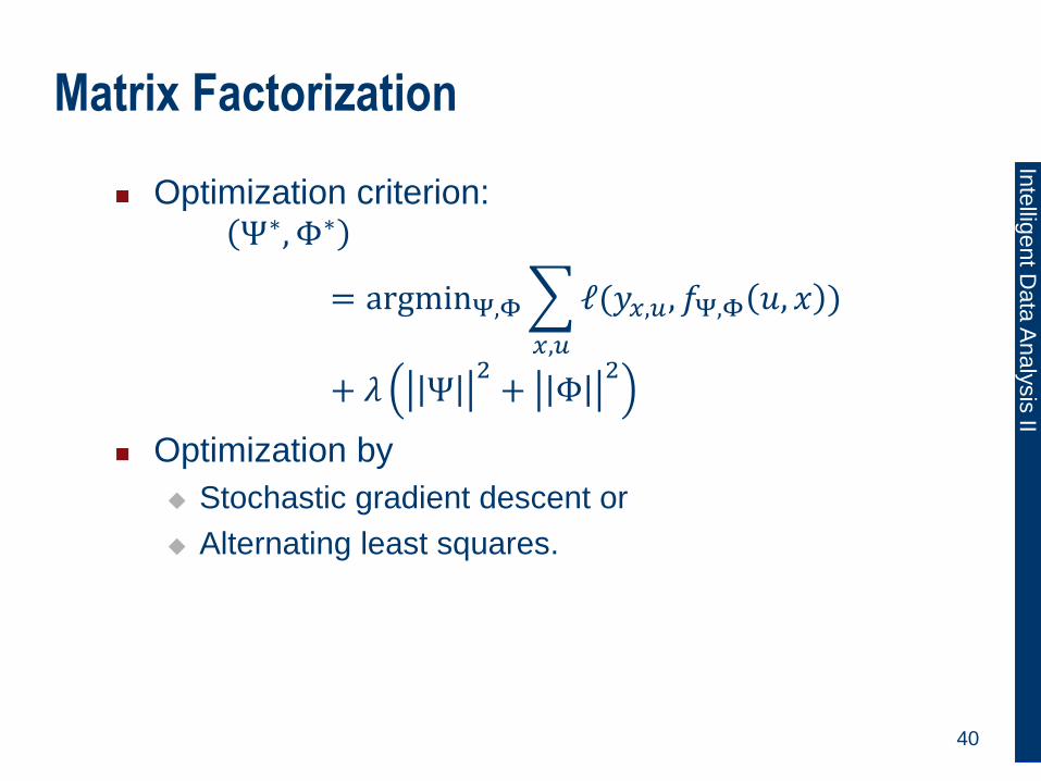
Matrix Factorization

Optimization criterion:

Ψ∗, Φ∗

= argminΨ,Φ ℓ(𝑦𝑥,𝑢,

𝑥,𝑢

𝑓Ψ,Φ 𝑢, 𝑥 )

+ 𝜆 Ψ2+ Φ

2

Optimization by

Stochastic gradient descent or

Alternating least squares.

40

Inte

lligent D

ata

Analy

sis

II

Matrix Factorization by Stochastic Gradient Descent

Iterate through ratings 𝑦𝑢,𝑥 in training sample

Let 𝜓𝑢′ ← 𝜓𝑢 − 𝛼

𝜕𝑓Ψ,Φ(𝑢,𝑥)

𝜕𝜓𝑢

Let 𝜙𝑥′ ← 𝜙𝑥 − 𝛼

𝜕𝑓Ψ,Φ(𝑢,𝑥)

𝜕𝜙𝑥

Until convergence.

Requires differentiable loss function; e.g., squared

loss, …

41

Inte

lligent D

ata

Analy

sis

II

Matrix Factorization by Alternating Least Squares

For squared loss and parallel architectures.

Alternate between 2 optimization processes:

Keep Φ fixed, optimize 𝜓𝑢 in parallel for all 𝑢.

Keep Ψ fixed, optimize 𝜙𝑥 in parallel for all 𝑥.

42

Inte

lligent D

ata

Analy

sis

II

Matrix Factorization by Alternating Least Squares

For squared loss and parallel architectures.

Alternate between 2 optimization processes:

Keep Φ fixed, optimize 𝜓𝑢 in parallel for all 𝑢.

Keep Ψ fixed, optimize 𝜙𝑥 in parallel for all 𝑥.

Optimization criterion for Ψ:

𝜓𝑢∗ = argmin𝜓𝑢

𝑦𝑢 − 𝑦 𝑢2 − 𝜆 𝜓𝑢

2

= argmin𝜓𝑢𝑦𝑢 − 𝜓𝑢

TΦT 2− 𝜆 𝜓𝑢

2

𝑦 𝑢1 … 𝑦 𝑢𝑚′ = 𝜓𝑢1 … 𝜓𝑢𝑘

𝜙11 … 𝜙𝑚′1

⋱𝜙1𝑘 𝜙𝑚′𝑘

43

Inte

lligent D

ata

Analy

sis

II

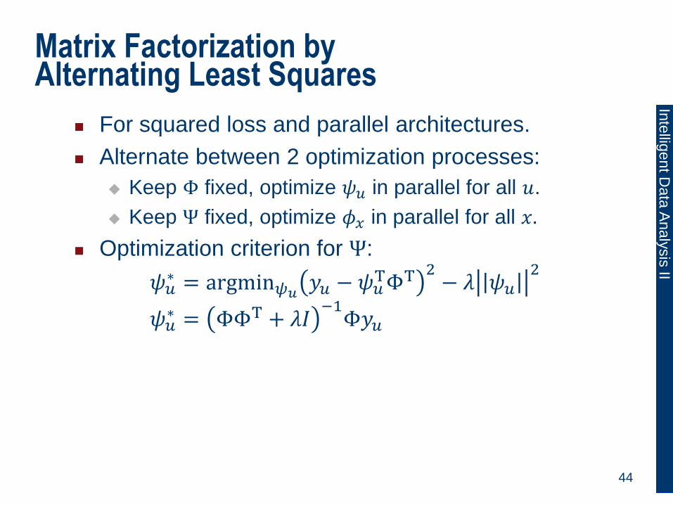
Matrix Factorization by Alternating Least Squares

For squared loss and parallel architectures.

Alternate between 2 optimization processes:

Keep Φ fixed, optimize 𝜓𝑢 in parallel for all 𝑢.

Keep Ψ fixed, optimize 𝜙𝑥 in parallel for all 𝑥.

Optimization criterion for Ψ:

𝜓𝑢∗ = argmin𝜓𝑢

𝑦𝑢 − 𝜓𝑢TΦT 2

− 𝜆 𝜓𝑢2

𝜓𝑢∗ = ΦΦT + 𝜆𝐼

−1Φ𝑦𝑢

44

Inte

lligent D

ata

Analy

sis

II

Matrix Factorization by Alternating Least Squares

For squared loss and parallel architectures.

Alternate between 2 optimization processes:

Keep Φ fixed, optimize 𝜓𝑢 in parallel for all 𝑢.

Keep Ψ fixed, optimize 𝜙𝑥 in parallel for all 𝑥.

Optimization criterion for Ψ:

𝜓𝑢∗ = argmin𝜓𝑢

𝑦𝑢 − 𝜓𝑢TΦT 2

− 𝜆 𝜓𝑢2

𝜓𝑢∗ = ΦΦT + 𝜆𝐼

−1Φ𝑦𝑢

Optimization criterion for Φ:

𝜙𝑥∗ = argmin𝜙𝑥

𝑦𝑥 − 𝜙𝑥TΨT 2

− 𝜆 𝜙𝑥2

𝜙𝑥∗ = ΨΨT + 𝜆𝐼

−1Ψ𝑦𝑥

45

Inte

lligent D

ata

Analy

sis

II

Matrix Factorization by Alternating Least Squares

For squared loss and parallel architectures.

Initialize Ψ, Φ randomly.

Repeat until convergence:

Keep Ψ fixed, for all 𝑢 in parallel:

𝜓𝑢 = ΦΦT + 𝜆𝐼−1

Φ𝑦𝑢

Keep Φ fixed, for all 𝑥 in parallel:

𝜙𝑢 = ΨΨT + 𝜆𝐼−1

Ψ𝑦𝑥

46

Inte

lligent D

ata

Analy

sis

II

Extensions: Biases

Some users just give optimistic or pessimistic

ratings; some items are hyped. Decision function: 𝑓Ψ,Φ,𝐵𝑢,𝐵𝑥

𝑢, 𝑥 = 𝑏𝑢 + 𝑏𝑥 + 𝜓𝑢T𝜙𝑥

Optimization criterion: Ψ∗, Φ∗, 𝐵𝑢, 𝐵𝑥

= argminΨ,Φ ℓ(𝑦𝑥,𝑢,

𝑥,𝑢

𝑓Ψ,Φ,𝐵𝑢,𝐵𝑥𝑢, 𝑥 )

+ 𝜆 Ψ2+ Φ

2+ 𝐵𝑢

2+ 𝐵𝑥

2

47

Inte

lligent D

ata

Analy

sis

II

Extensions: Explicit Features

Often, explicit user and item features are available.

Concatenate vectors 𝜓𝑢 and 𝜙𝑥; explicit features

are fixed, latent features are free paremeters.

48

Inte

lligent D

ata

Analy

sis

II

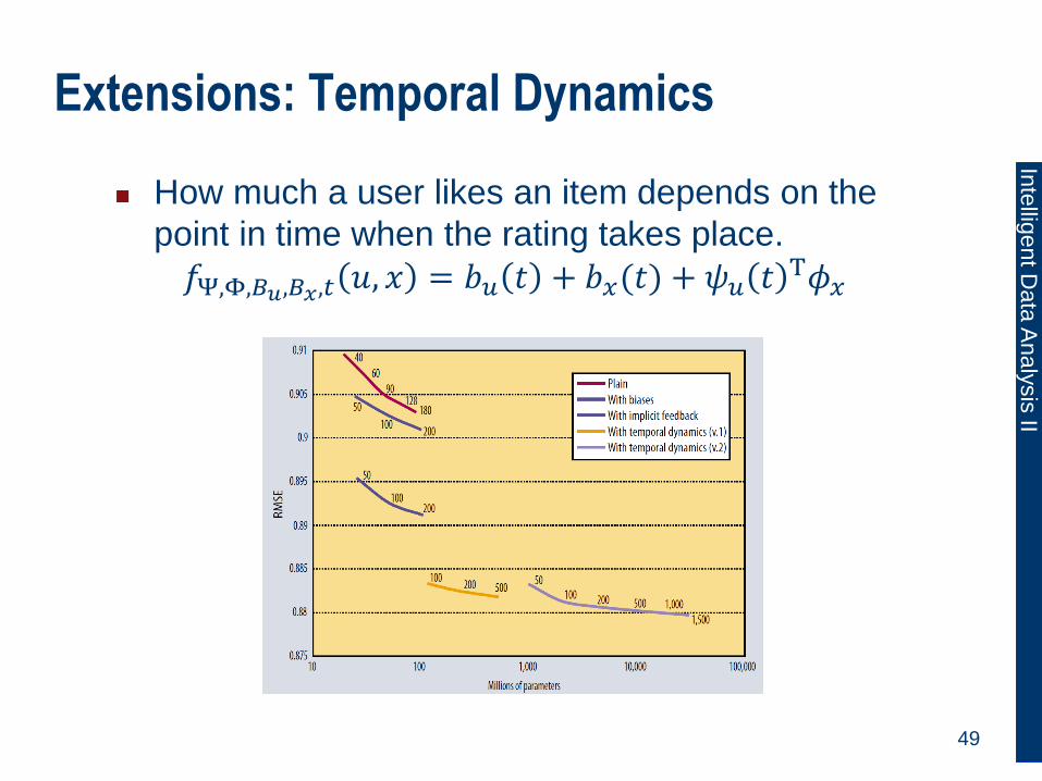
Extensions: Temporal Dynamics

How much a user likes an item depends on the

point in time when the rating takes place.

𝑓Ψ,Φ,𝐵𝑢,𝐵𝑥,𝑡 𝑢, 𝑥 = 𝑏𝑢 𝑡 + 𝑏𝑥(𝑡) + 𝜓𝑢 𝑡 T𝜙𝑥

49

Inte

lligent D

ata

Analy

sis

II

Summary

Purely content-based recommendation: users don‘t

benefit from other users‘ ratings.

Collaborative filtering by nearest neighbors: fixed

definition of similarity of users. No model

parameters, no learning. Has to iterate over data to

make recommendation.

Latent factor models, matrix factorization: user

preferences and item properties are free

parameters, optimized to minimized discrepancy

between inferred and actual ratings.

50