MASCThe Multiple Associative

Computing Model

Johnnie Baker, Jerry Potter, Robert Walker

Kent State University

(http://www.mcs.kent.edu/~parallel/)

MASC Model

2

OVERVIEW

• Introduction

– Motivation for the MASC model

– The MASC and ASC Models

– Languages Designed for the ASC Model

– Some ASC Algorithms and Programs

• ASC and MASC Algorithm Examples

– ASC version of Prim’s MST Algorithm

– ASC version of QUICKHULL

– MASC version of QUICKHULL.

• Simulations involving MASC (Overview)

– Background History and Basics

– Overview of PRAM Simulations

– Overview of Enhanced Mesh Simulations

– General Conclusions

MASC Model

3Motivation For MASC Model

• The STARAN Computer (Goodyear Aerospace, early 1970’s) provided an architectural model for associative computing.

• MASC provides a ‘definition’ for associative computing.

• Associative computing extends the data parallel paradigm to a complete computational model.

• Provides a platform for developing and comparing associative, MSIMD (Multiple SIMD) type programs.

• MASC is studied locally as a computational model (Baker), programming model (Potter), and architectural model (Baker, Potter, & Walker).

• Provides a practical model that supports massive parallelism.

• Model can also support intermediate parallel applications (e.g., multimedia computation, interactive graphics) using on-chip technology.

• Model addresses fact that most parallel applications are data parallel in nature, but contain several regions where significant branching occurs.

– Normally, at most eight active sub-branches.

• Provides a hybrid data-parallel, control-parallel model that can be compared to other parallel models.

MASC Model

4The MASC Model

Fig. 1 the MASC model

IS

CELL

NETWORK

IS

NETWORK

PEMemory

Cells

[1] [1] [2]

PEMemory

PEMemory

IS

• Basic Components– An array of cells, each consisting of a PE and its

local memory– An interconnection network between the cells– One or more instruction streams (ISs)– An IS communications network

• MASC is a MSIMD model that supports – both data and control parallelism– associative programming.

• MASC(n, j) is a MASC model with n PEs and j ISs

MASC Model

5

Basic Properties of MASC

• Instruction Streams or ISs

– A processor with a bus to each cell

– Each IS has a copy of the program and can broadcast instructions to cells in unit time

– NOTE: MASC(n,1) is called ASC

• Cell Properties– Each cell consists of a PE and its local memory– All cells listen to only one IS – Cells can switch ISs in unit time, based on a data

test.

– A cell can be active, inactive, or idle• Inactive cells listen but do not execute IS

commands• Idle cells contain no useful data and are

available for reassignment• Responder Processing

– An IS can detect if a data test is satisfied by any of its cells (each called a responder) in constant time

– An IS can select (or pick one) arbitrary responder in constant time.

– Justified by implementations using a resolver

MASC Model

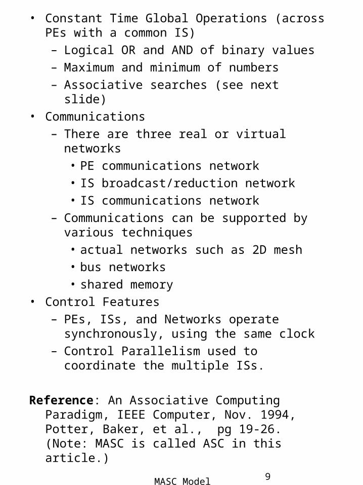
6• Constant Time Global Operations (across PEs with

a common IS)

– Logical OR and AND of binary values

– Maximum and minimum of numbers

– Associative searches (see next slide)

• Communications

– There are three real or virtual networks

• PE communications network

• IS broadcast/reduction network

• IS communications network

– Communications can be supported by various techniques

• actual networks such as 2D mesh

• bus networks

• shared memory

• Control Features

– PEs, ISs, and Networks operate synchronously, using the same clock

– Control Parallelism used to coordinate the multiple ISs.

Reference: An Associative Computing Paradigm, IEEE Computer, Nov. 1994, Potter, Baker, et al., pg 19-26. (Note: MASC is called ASC in this article.)

MASC Model

7

Dodge

Ford

Ford

Make

Subaru

Color

PE1

PE2

PE3

PE4

PE5

PE6

PE7

red

blue

white

red

Year

1994

1996

1998

1997

Model Price

Onlot

1

1

0

0

0

0

1

Busy-idle

1

0

1

1

0

0

1

IS

The Associative Search

MASC Model

8

Characteristics of Associative Programming

• Consistent use of data parallel programming

• Consistent use of global associative searching & responder processing

• Regular use of the constant time global reduction operations: AND, OR, MAX, MIN

• Data movement using IS bus broadcasts and IS fork and join operations to minimize the use of the PE network.

• Tabular representation of data

• Use of searching instead of sorting

• Use of searching instead of pointers

• Use of searching instead of ordering provided by linked lists, stacks, queues

• Promotes an intuitive type of programming that promotes high productivity

• Uses structure codes (i.e., numeric representation) to represent data structures such as trees, graphs, embedded lists, and matrices.

– See Nov. 1994 IEEE Computer article.

– Also, see Associative Computing by Potter

MASC Model

9

Languages Designed for MASC

• ASC was designed by Jerry Potter for MASC(n,1)

– Based on C and Pascal

– Initially designed as a parallel language.

– Avoids compromises required to extend an existing sequential language

• E.g., avoids unneeded sequential constructs such as pointers

– Implemented on several SIMD computers

• Goodyear Aerospace’s STARAN

• Goodyear/Loral’s ASPRO

• Thinking Machine’s CM-2

• WaveTracer

• ACE is a higher level language that uses natural language syntax; e.g., plurals, pronouns.

• Anglish is an ACE variant that uses an English-like grammar.

• An OOPs version of ASC for MASC(n,k) is planned (by Potter and his students)

• Language Refs: www.mcs.kent.edu/~potter/ and Jerry Potter, Associative Computing - A Programming Paradigm for Massively Parallel Computers, Plenum Publishing Company, 1992

MASC Model

10

Algorithms and Programs Implemented in ASC

• A wide range of algorithms implemented in ASC without use of PE network

– Graph Algorithms

• minimal spanning tree

• shortest path

• connected components

– Computational Geometry Algorithms

• convex hull algorithms (Jarvis March, Quickhull, Graham Scan, etc)

• Dynamic hull algorithms

– String Matching Algorithms

• all exact substring matches

• all exact matches with “don’t care” (i.e., wild card) characters.

– Algorithms for NP-complete problems

• traveling salesperson

• 2-D knapsack.

– Data Base Management Software

• associative data base

• relational data base

MASC Model

11

(Cont) ASC Algorithms and Programs

– A Two Pass Compiler for ASC

• first pass

• optimization phase

– Two Rule-Based Inference Engines

• OPS-5 interpreter

• PPL (Parallel Production Language interpreter)

– A Context Sensitive Language Interpreter

• (OPS-5 variables force context sensitivity)

– An associative PROLOG interpreter

• Numerous Programs in ASC using a PE network

– 2-D Knapsack Algorithm using a 1-D mesh

– Image Processing algorithms using 1-D mesh

– FFT using Flip Network

– Matrix Multiplication using 1-D mesh

– An Air Traffic Control Program using Flip Network

• Demonstrated using live data at Knoxville in mid 70’s.

MASC Model

12

Preliminaries for MST Algorithm

• Next, a “data structure” level presentation of Prim’s algorithm for the MST is given.

• The data structure used is illustrated in the example in Figure 6 on slide 15.

– Figure 6 is from the basic paper in Nov. 1994 IEEE Computer (see slide 6).

• There are two types of variables for the ASC model, namely

– the parallel variables (i.e., ones for the PEs)

– the scalar variables (ie., the ones for the control unit).

– Scalar variables are essentially global variables.

• Can replace each with a parallel variable.

• In order to distinguish between them, the parallel variables names end with a “$” symbol.

• Each step in this algorithm is constant.

• One MST edge is selected during each pass through the loop in this algorithm.

• Since a spanning tree has n-1 edges, the running time of this algorithm is O(n).

• Since the sequential running time of the Prim MST algorithm is O(n 2) and this time is optimal, this parallel implementation is cost-optimal.

MASC Model

13

Algorithm: ASC-MSP-PRIM(root)

• Initially assign any node to root.

• All processors set

– candidate$ to “waiting”

– current-best$ to – the candidate field for the root node to “no”

• All processors whose distance d from their node to root node is finite do

– Set their candidate$ field to “yes

– Set their parent$ field to root.

– Set current_best$ = d.

• While the candidate field of some processor is “yes”,

– Restrict the active processors to those responding and (for these processors) do

• Compute the minimum value x of current_best$.

• Restrict the active processors to those with current_best$ = x and do

– pick an active processor, say one with node y.

» Set the candidate$ value of this processor to “no”

– Set the scalar variable next-node to y.

MASC Model

14

– If the value z in the next_node field of a processor is less than current_best$, then

» Set current_best$ to z.

– Set parent$ to next_node

• For all processors, if candidate$ is “waiting” and the distance of its node from next_node is finite, then

– Set candidate$ to “yes”

– Set parent$ to next-node

– Set current_best$ to the distance of its node from next_node.

COMMENTS:

• Figure 6 on the next slide shows the data structure used in the preceding ASC algorithm for MST

• Next slide is from the Nov 1994 IEEE Computer paper referenced earlier.

– This slide also gives a compact, data-structures level pseudo-code description for this algorithm

• Pseudo-code illustrates Potter’s use of pronouns (e.g., them)

• The mindex function returns the index of a processor holding the minimal value.

– This MST pseudo-code is much simpler than data-structure level sequential MST pseudo-codes (e.g., Sara Baase’s algorithm textbook).

MASC Model

15

Slides from Maher’s Work Go Here

• First slide of Figure 6 in the IEEE Computer article on associative minimal spanning tree goes here. (Don’t number this slide, as it would be slide 15.

• Next use slides 15 - 23 from my general presentations (prepared by Maher) called “An Associative Model of Computation”. It is in latex and in directory ~jbaker/slides/matwah in UNIX directory.

• I am adding blank slides 16-23 to keep numbering correct.

• Work starting with slide 24 on simulations between enhanced meshes and MASC in dissertation work of Mingxian Jin.

MASC Model

16

MASC Model

17

MASC Model

18

MASC Model

19

MASC Model

20

MASC Model

21

MASC Model

22

MASC Model

23

MASC Model

24

Previous MASC Simulation

• MASC Simulation of PRAM

– MASC(n,j) can simulate priority CRCW PRAM(n,m) in O(min{n/j, m/j}) with high probability.

– MASC(n,1) [or ASC] can simulate priority CRCW with a constant number of global memory locations in constant time

• This result is stronger than it first appears

• Some CRCW algorithms only require a constant nr of global memory locations

– A reverse simulation of MASC by Combining CRCW PRAM result will be in the dissertation of Mingxian Jin

• Self-simulation of MASC

– Provides an efficient algorithm for MASC to efficiently simulate a larger MASC - with more PEs and/or ISs.

– Establishes that MASC is highly scalable

– MASC(n,j) can simulate MASC(N,J) in O(N/n + J) extra time and O(N/n + J) extra memory.

MASC Model

25

The Enhanced Mesh, MMB

• Enhanced meshes are basic mesh models augmented with fixed or reconfigurable buses

– At most one PE on a bus can broadcast to remaining PEs during one step.

• Best-known fixed bus example:

– Mesh with multiple broadcasting (MMB)

– Standard 2-D mesh

– Row and column bus enhancements

– Broadcasts can occur along only row or column buses (but not both) in one step

MASC Model

26

N

W E

S

The Reconfigurable Enhanced Mesh RM

• For all reconfigurable bus models, buses are created dynamically during execution

• Best known example:

– General Reconfigurable Mesh (RM)

– Each PE has four ports called N,S, E, W (often called “NEWS”)

– In one step, each PE can set the connections of its ports, based on local data

– At most two disjoint pairs of ports can be connected at any time

– One such connection is the adjacent pairs,

{{N,E}, {W,S}}.

MASC Model

27

Simulation Preliminaries

• Reasons to simulate other models using MASC

– Allows a better understanding of the power of MASC

– Provides a simulation algorithm that can be used to convert algorithms designed for the other model to MASC

• Basic Assumption Used in the Simulations

– MASC(n, ) has a mesh PE network with row-major ordering

– The enhanced meshes have a 2D mesh with the same size and ordering

– Each PE in MASC has the same computational power as an enhanced mesh PE

– The MASC buses have the same power as the buses of the enhanced mesh

– Word length of both models are lg(n).– Each PE in MASC knows its position in the 2D

mesh.

nn n

MASC Model

28

Simulation Mappings between MASC & Enhanced Meshes

IS1

IS2

ISj

Cell Cell

CellCell Cell

Cell

C e l l N e t w o r k

I S N e t w o r k

• The mapping is between MASC(n, ) and Enhanced meshes of size

• The mapping assigns a PE in one model to the PE that is in the same position in the 2D mesh in the other model

• The ith IS in MASC simulates both the ith row and the ith column buses

nnn nn

MASC Model

29

Simulation of MMB with MASC

• Since both models have identical 2D meshes, these do not need to be simulated

• Since the power of PEs in respective models are identical, their local computations are not simulated

• To simulate a MMB row broadcast on the MASC,

– All PEs switch to their assigned row IS

– The IS for each row checks to see if there is a PE that wishes to broadcast

– If true, the IS broadcasts this value to all of its PEs (i.e., the ones on its assigned row).

• Simulation of a MMB column broadcast is similar

• The running time is O(1)

• There are examples that show the MASC model is strictly more powerful than the MMB model

Theorem 1.

• MASC(n, j) with a 2-D mesh is strictly more powerful than a MMB for j = ( ).

• An algorithm for a MMB can be executed on MASC(n, j) with j=( ) and a 2-D mesh with a running time at least fast as the MMB time.

nn n

nnn

MASC Model

30

Simulation of MASC by MMB

• PE(1,1) stores a copy of the program and simulates the ISs sequentially.

• Each instruction stream command or datum is first sent by P(1,1) to the PEs in the first column.

• Next, the PEs in the first column broadcast this command or datum along the rows to all PEs.

• Each MMB processor uses two registers, channel and status, to decide whether or not to execute the current instruction.– channel records which IS the processor is assigned to– status records whether PE is active, inactive, etc

• The simulation of simultaneous broadcasts of ISs takes O( ) time.

• A local computation, memory access, or a data movement along local links are identical in the two models and require O(1) time.

• The execution of a global reduction operator OR, AND, MAX, MIN takes O( ) using an optimal MMB algorithm.

• Since the global reduction operators may be computed for O( ) ISs, an upper bound is O( ) or O( ).

Theorem 3.• MASC(n, ) with a 2-D mesh can be simulated

by a MMB in O( ) time with O( ) extra memory

n

n

n

n 32

n 61

nn 61n

nn

n 32

n

n

MASC Model

31

Conclusions

• MASC is strictly more powerful than an MMB of the same size.

• Any algorithm for an MMB can be executed on a MASC of the same size with the same running time. In particular,

– Optimal algorithms for MMB are also optimal when executed on MASC

• CLAIM: MASC and RM are dissimilar and can not simulate each other efficiently. n