
MAS309 Coding theory - QMUL Mathsmj/MAS309/lectureNotes.pdf · 2 Coding Theory 6 Some examples of...
50
MAS309 Coding theory Matthew Fayers January–March 2008 This is a set of notes which is supposed to augment your own notes for the Coding Theory course. They were written by Matthew Fayers, and very lightly edited my me, Mark Jerrum, for 2008. I am very grateful to Matthew Fayers for permission to use this excellent material. If you find any mistakes, please e-mail me: [email protected]. Thanks to the following people who have already sent corrections: Nilmini Herath, Julian Wiseman, Dilara Azizova. Contents 1 Introduction and definitions 2 1.1 Alphabets and codes .................................. 2 1.2 Error detection and correction ............................. 2 1.3 Equivalent codes .................................... 4 2 Good codes 6 2.1 The main coding theory problem ............................ 6 2.2 Spheres and the Hamming bound ............................ 8 2.3 The Singleton bound .................................. 9 2.4 Another bound ..................................... 10 2.5 The Plotkin bound .................................... 11 3 Error probabilities and nearest-neighbour decoding 13 3.1 Noisy channels and decoding processes ........................ 13 3.2 Rates of transmission and Shannon’s Theorem ..................... 15 4 Linear codes 15 4.1 Revision of linear algebra ................................ 16 4.2 Finite fields and linear codes .............................. 18 4.3 The minimum distance of a linear code ......................... 19 4.4 Bases and generator matrices .............................. 20 4.5 Equivalence of linear codes ............................... 21 4.6 Decoding with a linear code .............................. 27 5 Dual codes and parity-check matrices 30 5.1 The dual code ...................................... 30 5.2 Syndrome decoding ................................... 34 1
Transcript of MAS309 Coding theory - QMUL Mathsmj/MAS309/lectureNotes.pdf · 2 Coding Theory 6 Some examples of...
MAS309 Coding theory
Matthew Fayers
January–March 2008
This is a set of notes which is supposed to augment your own notes for the Coding Theory course.They were written by Matthew Fayers, and very lightly edited my me, Mark Jerrum, for 2008. I amvery grateful to Matthew Fayers for permission to use this excellent material. If you find any mistakes,please e-mail me: [email protected]. Thanks to the following people who have already sentcorrections: Nilmini Herath, Julian Wiseman, Dilara Azizova.
Contents
1 Introduction and definitions 21.1 Alphabets and codes . . . . . . . . . . . . . . . . . . . . . . . . . . . . . . . . . . 21.2 Error detection and correction . . . . . . . . . . . . . . . . . . . . . . . . . . . . . 21.3 Equivalent codes . . . . . . . . . . . . . . . . . . . . . . . . . . . . . . . . . . . . 4
2 Good codes 62.1 The main coding theory problem . . . . . . . . . . . . . . . . . . . . . . . . . . . . 62.2 Spheres and the Hamming bound . . . . . . . . . . . . . . . . . . . . . . . . . . . . 82.3 The Singleton bound . . . . . . . . . . . . . . . . . . . . . . . . . . . . . . . . . . 92.4 Another bound . . . . . . . . . . . . . . . . . . . . . . . . . . . . . . . . . . . . . 102.5 The Plotkin bound . . . . . . . . . . . . . . . . . . . . . . . . . . . . . . . . . . . . 11
3 Error probabilities and nearest-neighbour decoding 133.1 Noisy channels and decoding processes . . . . . . . . . . . . . . . . . . . . . . . . 133.2 Rates of transmission and Shannon’s Theorem . . . . . . . . . . . . . . . . . . . . . 15
4 Linear codes 154.1 Revision of linear algebra . . . . . . . . . . . . . . . . . . . . . . . . . . . . . . . . 164.2 Finite fields and linear codes . . . . . . . . . . . . . . . . . . . . . . . . . . . . . . 184.3 The minimum distance of a linear code . . . . . . . . . . . . . . . . . . . . . . . . . 194.4 Bases and generator matrices . . . . . . . . . . . . . . . . . . . . . . . . . . . . . . 204.5 Equivalence of linear codes . . . . . . . . . . . . . . . . . . . . . . . . . . . . . . . 214.6 Decoding with a linear code . . . . . . . . . . . . . . . . . . . . . . . . . . . . . . 27
5 Dual codes and parity-check matrices 305.1 The dual code . . . . . . . . . . . . . . . . . . . . . . . . . . . . . . . . . . . . . . 305.2 Syndrome decoding . . . . . . . . . . . . . . . . . . . . . . . . . . . . . . . . . . . 34
1
2 Coding Theory
6 Some examples of linear codes 366.1 Hamming codes . . . . . . . . . . . . . . . . . . . . . . . . . . . . . . . . . . . . . 376.2 Existence of codes and linear independence . . . . . . . . . . . . . . . . . . . . . . 416.3 MDS codes . . . . . . . . . . . . . . . . . . . . . . . . . . . . . . . . . . . . . . . 446.4 Reed–Muller codes . . . . . . . . . . . . . . . . . . . . . . . . . . . . . . . . . . . 47
1 Introduction and definitions
1.1 Alphabets and codes
In this course, we shall work with an alphabet, which is simply a finite set A of symbols. If Ahas size q, then we call A a q-ary alphabet (although we say binary and ternary rather than 2-aryand 3-ary). For most purposes, it is sufficient to take A to be the set {0, 1, . . . , q − 1}. Later we shallspecialise to the case where q is a prime power, and take A to be Fq, the field of order q.
A word of length n is simply a string consisting of n (not necessarily distinct) elements of A, i.e.an element of An, and a block code of length n is simply a set of words of length n, i.e. a subset of An.If A is a q-ary alphabet, we say that any code over A is a q-ary code. There are codes in which thewords have different lengths, but in this course we shall be concerned entirely with block codes, andso we refer to these simply as codes. We refer to the words in a code as the codewords.
1.2 Error detection and correction
Informally, a code is t-error-detecting if, whenever we take a codeword and change at most t of thesymbols in it, we don’t reach a different codeword. So if we send the new word to someone withouttelling him which symbols we changed, he will be able to tell us whether we changed any symbols.
A code is t-error-correcting if whenever we take a codeword and change at most t of the symbolsin it, we don’t reach a different codeword, and we don’t even reach a word which can be obtainedfrom a different starting codeword by changing at most t of the symbols. So if we send the new wordto someone without telling him which symbols we changed, he will be able to tell us which codewordwe started with.
Formally, we define a metric (or distance function) on An as follows: given two words x and y, wedefine d(x, y) to be the number of positions in which x and y differ, i.e. if x = x1 . . . xn and y = y1 . . . yn,then d(x, y) is the number of values i for which xi , yi. This distance function is called the Hammingdistance.
Lemma 1.1. d is a metric on An, i.e.:
1. d(x, x) = 0 for all x ∈ An;
2. d(x, y) > 0 for all x , y ∈ An;
3. d(x, y) = d(y, x) for all x, y ∈ An;
4. (the triangle inequality) d(x, z) 6 d(x, y) + d(y, z) for all x, y, z ∈ An.
Proof. (1), (2) and (3) are very easy, so let’s do (4). Now d(x, z) is the number of values i for whichxi , zi. Note that if xi , zi, then either xi , yi or yi , zi. Hence
{i | xi , zi} ⊆ {i | xi , yi} ∪ {i | yi , zi}.
Introduction and definitions 3
So
{|i | xi , zi}| 6 |{i | xi , yi} ∪ {i | yi , zi}|
6 |{i | xi , yi}| + |{i | yi , zi}|,
i.e.d(x, z) 6 d(x, y) + d(y, z).
�
Now we can talk about error detection and correction. We say that a code C is t-error detectingif d(x, y) > t for any two distinct words in C. We say that C is t-error-correcting if there do not existwords x, y ∈ C and z ∈ An such that d(x, z) 6 t and d(y, z) 6 t.
Example. The simplest kinds of error-detecting codes are repetition codes. The repetition code oflength n over A simply consists of all words aa . . . a, for a ∈ A. For this code, any two distinctcodewords differ in every position, and so d(x, y) = n for all x , y in C. So the code is t-error-detecting for every t 6 n − 1, and is t-error-correcting for every t 6 n−1
2 .
Given a code C, we define its minimum distance d(C) to be the smallest distance between distinctcodewords:
d(C) = min{d(x, y) | x , y ∈ C}.
Lemma 1.2. A code C is t-error-detecting if and only if d(C) > t + 1, and is t-error-correcting if andonly if d(C) > 2t + 1,
Proof. The first part is immediate from the definition of “t-error-detecting”. For the second part,assume that C is not t-error-correcting. Then there exist distinct codewords x, y ∈ C and and a wordz ∈ An such that d(x, z) ≤ t and d((y, z) ≤ t. By the triangle inequality, d(x, y) ≤ d(x, z) + d((y, z) ≤ 2t,and hence d(C) ≤ 2t. Conversely, if d(C) ≤ 2t then choose x, y ∈ C such that d(x, y) ≤ 2t. There existsz ∈ An such that d(x, z) ≤ t and d((y, z) ≤ t. (Check this! It is a property of the Hamming metric, butnot of metrics in general.) Thus, C is not t-error-correcting. �
Corollary 1.3. A code C is t-error-correcting if and only if it is (2t)-error-detecting.
Proof. By the previous lemma, the properties “t-error-correcting” and “2t-error-detecting” for thecode C are both equivalent to d(C) ≥ 2t + 1. �
From now on, we shall think about the minimum distance of a code rather than how many errorsit can detect or correct.
We say that a code of length n with M codewords and minimum distance at least d is an (n,M, d)-code. For example, the repetition code described above is an (n, q, n)-code. Another example is thefollowing ‘parity-check’ code, which is a binary (4, 8, 2)-code:
{0000, 0011, 0101, 0110, 1001, 1010, 1100, 1111}.
The point of using error-detecting and error-correcting codes is that we might like to transmit amessage over a ‘noisy’ channel, where each symbol we transmit gets mis-transmitted with a certainprobability; an example (for which several of the codes we shall see have been used) is a satellite

4 Coding Theory
transmitting images from the outer reaches of the solar system. Using an error-detecting code, wereduce the probability that the receiver misinterprets distorted information – provided not too manyerrors have been made in transmission, the receiver will know that errors have been made, and canrequest re-transmission; in a situation where re-transmission is impractical, an error-correcting codecan be used. Of course, the disadvantage of this extra ‘certainty’ of faithful transmission is that we areadding redundant information to the code, and so our message takes longer to transmit. In addition,for intricate codes, decoding may be difficult and time-consuming.
The main tasks of coding theory, therefore, are to find codes which enable error-detection and-correction while adding as little redundant information as possible, and to find efficient decodingprocedures for these codes. Clearly, as d gets large, codes with minimum distance d have fewer andfewer codewords. So we try to find codes of a given length and a given minimum distance which haveas many codewords as possible. We shall see various bounds on the possible sizes of codes with givenlength and minimum distance, and also construct several examples of ‘good’ codes.
1.3 Equivalent codes
To simplify our study of codes, we introduce a notion of equivalence of codes. If C and D arecodes of the same length over the same alphabet, we say that C is equivalent to D if we can get fromC toD by a combination of the following operations.
Operation 1 – permutation of the positions in the codewords Choose a permutationσ of {1, . . . , n},and for a codeword v = v1 . . . vn in C define
vσ = vσ(1) . . . vσ(n).
Now defineCσ = {vσ | v ∈ C}.
Operation 2 – applying a permutation of A in a fixed position in the codewords Choose a permu-tation f of A and an integer i ∈ {1, . . . , n}, and for v = v1 . . . vn define
v f ,i = v1, . . . , vi−1 f (vi)vi+1 . . . vn.
Now defineC f ,i = {v f ,i | v ∈ C}.
For example, consider the following ternary codes of length 2:
C = {10, 21, 02}, D = {01, 12, 20}, E = {00, 11, 22}.
We can from C toD by Operation 1 – we replace each codeword ab with ba. We can get fromD to Eby Operation 2 – we permute the symbols appearing in the second position via 0 → 2 → 1 → 0. SoC,D and E are equivalent codes.
The point of equivalence is that equivalent codes have the same size and the same minimumdistance; we can often simplify both decoding procedures and some of our proofs by replacing codeswith equivalent codes.
Lemma 1.4. Suppose C is a code and σ a permutation of {1, . . . , n}, and define Cσ as above. Then|C| = |Cσ|.

Introduction and definitions 5
Proof. The mapv 7→ vσ
defines a function from C to Cσ, and we claim that this is a bijection. Surjectivity is immediate: Cσis defined to be the image of the function. For injectivity, suppose that v = v1 . . . vn and w = w1 . . .wn
are codewords in C with v , w. This means that v j , w j for some j. Since σ is a permutation, wehave j = σ(i) for some i, and so vσ and wσ differ in position i, so are distinct. �
Lemma 1.5. Suppose C is a code containing words v and w, and suppose σ is a permutation of{1, . . . , n}. Define the words vσ and wσ as above. Then
d(vσ,wσ) = d(v,w).
Proof. Write v = v1 . . . vn, w = w1 . . .n, vσ = x1 . . . xn, wσ = y1 . . . yn. Then by definition we havexi = vσ(i) and yi = wσ(i) for each i. Now d(v,w) is the number of positions in which v and w differ, i.e.
d(v,w) = |{i | vi , wi}|;
similarly,d(vσ,wσ) = |{i | xi , yi}|.
Since xi = vσ(i) and yi = wσ(i), σ defines a bijection from
{i | xi , yi}
to{i | vi , wi}.
�
Corollary 1.6. Define Cσ as above. Then d(Cσ) = d(C).
Now we prove the same properties for Operation 2.
Lemma 1.7. Suppose C is a code, f a permutation of A and i ∈ {1, . . . , n}, and define C f ,i as above.Then |C f ,i| = |C|.
Proof. The mapv 7→ v f ,i
defines a function from C to C f ,i, and we claim that this is a bijection. Surjectivity follows by definitionof C f ,i. For injectivity, suppose that v,w are codewords in C with v , w. There is some j ∈ {1, . . . , n}with v j , w j. If j = i, then f (vi) , f (w j) (since f is a permutation), and so v f ,i and w f ,i differ inposition i. If j , i, then v f ,i and w f ,i differ in position j. �
Lemma 1.8. Suppose C is a code containing codewords v and w, and define v f ,i and w f ,i as above.Then
d(v f ,i,w f ,i) = d(v,w).
6 Coding Theory
Proof. Write v = v1 . . . vn and w = w1 . . .wn. If vi = wi, then f (vi) = f (wi), so
d(v,w) = |{ j , i | vi , wi}| = d(v f ,i,w f ,i).
If vi , wi, then (since f is a permutation) f (vi) , f (wi), and so
d(v,w) = |{ j , i | vi , wi}| + 1 = d(v f ,i,w f ,i).
�
Corollary 1.9. Define C f ,i as above. Then d(C f ,i) = d(C).
One of the reasons for using equivalent codes is that they enable us to assume that certain wordslie in our codes.
Lemma 1.10. Suppose C is a non-empty code over A, and a ∈ A. Then C is equivalent to a codecontaining the codeword aa . . . a.
Proof. We prove a stronger statement by induction. For i ∈ {0, . . . , n} let P(i) denote the statement ‘Anon-empty code C is equivalent to a code containing a word v = v1 . . . vn with v1 = · · · = vi = a’.
P(0) is true: any code is equivalent to itself, and we may take any v. Now suppose i > 0 and thatP(i−1) is true. So C is equivalent to a codeD containing a word v = v1 . . . vn with v1 = · · · = vi−1 = a.Choose any permutation f of A for which f (vi) = a. Then D is equivalent to the code D f ,i, whichcontains the word v f ,i, whose first i entries equal a, and C is equivalent toD f ,i as well.
By induction, P(n) is true, which is what we want. �
2 Good codes
2.1 The main coding theory problem
The most basic question we might ask about codes is: given n, M and d, does an (n,M, d)-codeexist? Clearly, better codes are those which make M and d large relative to n, so we define Aq(n, d)to be the maximum M such that a q-ary (n,M, d)-code exists. The numbers Aq(n, d) are unknown ingeneral, and calculating them is often referred to as the ‘main coding theory problem’. Here are twovery special cases.
Theorem 2.1.
1. Aq(n, 1) = qn.
2. Aq(n, n) = q.
Proof.1. We can take C = An, the set of all words of length n. Any two distinct words must differ in
at least one position, so the code has minimum distance at least 1. Obviously a q-ary code oflength n can’t be bigger than this.
2. Suppose we have a code of length n with at least q + 1 codewords. Then by the pigeonholeprinciple there must be two words with the same first symbol. These two words can thereforediffer in at most n−1 positions, and so the code has minimum distance less than n. So Aq(n, n) 6q. On the other hand, the repetition code described above is an (n, q, n)-code.

Good codes 7
�
Here is a less trivial example.
Theorem 2.2.A2(5, 3) = 4.
Proof. It is easily checked that the following binary code is (5, 4, 3):
{00000, 01101, 10110, 11011}.
So A2(5, 3) > 4. Now suppose C is a binary code of length 5 with minimum distance at least 3 and atleast five codewords. By replacing C with an equivalent code and appealing to Lemma 1.10, we mayassume that C contains the codeword 00000. Since C has minimum distance at least 3, every remain-ing codeword must contain at least three 1s. If there are two codewords x, y each with at least four 1s,then d(x, y) 6 2, which gives a contradiction, so there must be at least three codewords with exactlythree 1s. Trial and error shows that two of these must be distance at most 2 apart; contradiction. �
Now we come to our first non-trivial result. It is a ‘reduction theorem’, which in effect says thatfor binary codes we need only consider codes with odd values of d.
Theorem 2.3. Suppose d is even. Then a binary (n,M, d)-code exists if and only if a binary (n −1,M, d − 1)-code exists.
Hence if d is even, then A2(n, d) = A2(n − 1, d − 1).
Proof. The ‘only if’ part follows from the Singleton bound, which we state and prove in Section 2.3.So we concentrate on the ‘if’ part.
Suppose we have a binary (n− 1,M, d− 1)-code. Given a codeword x, we form a word x of lengthn by adding an extra symbol, which we choose to be 0 or 1 in such a way that x contains an evennumber of 1s.
Claim. If x, y are codewords in C, then d(x, y) is even.
Proof. The number of positions in which x and y differ is
(number of places where x has a 1 and y has a 0)
+(number of places where x has a 0 and y has a 1)
which equals
(number of places where x has a 1 and y has a 0)
+(number of places where x has a 1 and y has a 1)
+(number of places where x has a 0 and y has a 1)
+(number of places where x has a 1 and y has a 1)
−2(number of places where x has a 1 and y has a 1)
which equals
(number of places where x has a 1)
+(number of places where y has a 1)
−2(number of places where x has a 1 and y has a 1)
which is the sum of three even numbers, so is even.

8 Coding Theory
Now for any x, y ∈ C, we have d(x, y) > d − 1, and clearly this gives d(x, y) > d − 1. But d − 1 isodd, and d(x, y) is even, so in fact we have d(x, y) > d. So the code
C = {x | x ∈ C}
is an (n,M, d)-code.For the final part of the theorem, we have
A2(n, d) = max{M | a binary (n,M, d)-code exists}
= max{M | a binary (n − 1,M, d − 1)-code exists}
= A2(n − 1, d − 1).
�
Now we’ll look at some upper bounds for sizes of (n,M, d)-codes.
2.2 Spheres and the Hamming bound
Since the Hamming distance d makes An into a metric space, we can define the sphere around anyword. If x ∈ An is a word, then the sphere of radius r and centre x is
S (x, r) = {y ∈ An | d(x, y) 6 r}.
(n.b. in metric-space language this is a ball, but the word ‘sphere’ is always used by coding-theorists.)The importance of spheres lies in the following lemma.
Lemma 2.4. A code C is t-error-correcting if and only if for any distinct words x, y ∈ C, the spheresS (x, t) and S (y, t) are disjoint.
This lemma gives us a useful bound on the size of a t-error-correcting code. We begin by countingthe words in a sphere; recall the binomial coefficient
(nr
)= n!
(n−r)!r! .
Lemma 2.5. If A is a q-ary alphabet, x is a word over A of length n and r 6 n, then the sphere S (x, r)contains exactly (
n0
)+ (q − 1)
(n1
)+ (q − 1)2
(n2
)+ · · · + (q − 1)r
(nr
)words.
Proof. We claim that for any i, the number of words y such that d(x, y) equals i is (q − 1)i(ni
); the
lemma then follows by summing for i = 0, 1, . . . , r.d(x, y) = i means that x and y differ in exactly i positions. Given x, in how many ways can we
choose such a y? We begin by choosing the i positions in which x and y differ; this can be done in(ni
)ways. Then we choose what symbols will appear in these i positions in y. For each position, we
can choose any symbol other than the symbol which appears in that position in x – this gives us q − 1choices. So we have (q − 1)i choices for these i symbols altogether. �
Theorem 2.6 (Hamming bound). If C is a t-error-correcting code of length n over a q-ary alphabetA, then
|C| 6qn(
n0
)+ (q − 1)
(n1
)+ (q − 1)2
(n2
)+ · · · + (q − 1)t
(nt
) .
Good codes 9
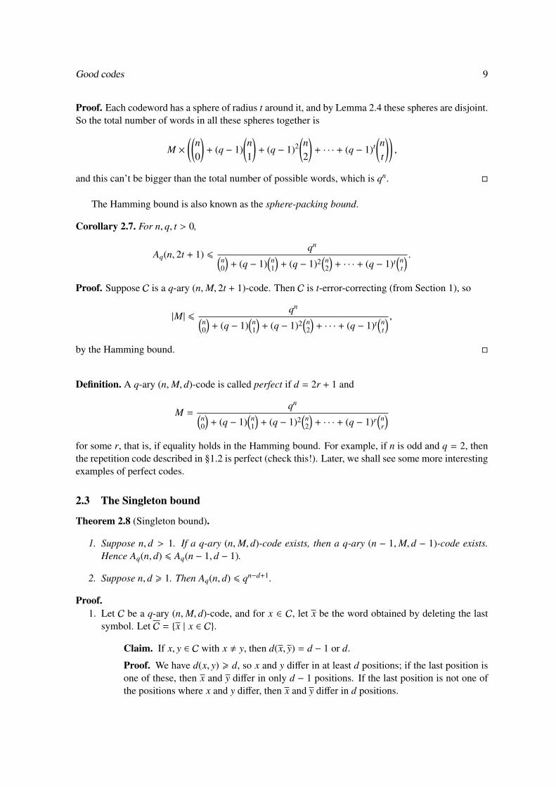
Proof. Each codeword has a sphere of radius t around it, and by Lemma 2.4 these spheres are disjoint.So the total number of words in all these spheres together is
M ×((
n0
)+ (q − 1)
(n1
)+ (q − 1)2
(n2
)+ · · · + (q − 1)t
(nt
)),
and this can’t be bigger than the total number of possible words, which is qn. �
The Hamming bound is also known as the sphere-packing bound.
Corollary 2.7. For n, q, t > 0,
Aq(n, 2t + 1) 6qn(
n0
)+ (q − 1)
(n1
)+ (q − 1)2
(n2
)+ · · · + (q − 1)t
(nt
) .Proof. Suppose C is a q-ary (n,M, 2t + 1)-code. Then C is t-error-correcting (from Section 1), so
|M| 6qn(
n0
)+ (q − 1)
(n1
)+ (q − 1)2
(n2
)+ · · · + (q − 1)t
(nt
) ,by the Hamming bound. �
Definition. A q-ary (n,M, d)-code is called perfect if d = 2r + 1 and
M =qn(
n0
)+ (q − 1)
(n1
)+ (q − 1)2
(n2
)+ · · · + (q − 1)r
(nr
)for some r, that is, if equality holds in the Hamming bound. For example, if n is odd and q = 2, thenthe repetition code described in §1.2 is perfect (check this!). Later, we shall see some more interestingexamples of perfect codes.
2.3 The Singleton bound
Theorem 2.8 (Singleton bound).
1. Suppose n, d > 1. If a q-ary (n,M, d)-code exists, then a q-ary (n − 1,M, d − 1)-code exists.Hence Aq(n, d) 6 Aq(n − 1, d − 1).
2. Suppose n, d > 1. Then Aq(n, d) 6 qn−d+1.
Proof.1. Let C be a q-ary (n,M, d)-code, and for x ∈ C, let x be the word obtained by deleting the last
symbol. Let C = {x | x ∈ C}.
Claim. If x, y ∈ C with x , y, then d(x, y) = d − 1 or d.
Proof. We have d(x, y) > d, so x and y differ in at least d positions; if the last position isone of these, then x and y differ in only d − 1 positions. If the last position is not one ofthe positions where x and y differ, then x and y differ in d positions.
10 Coding Theory
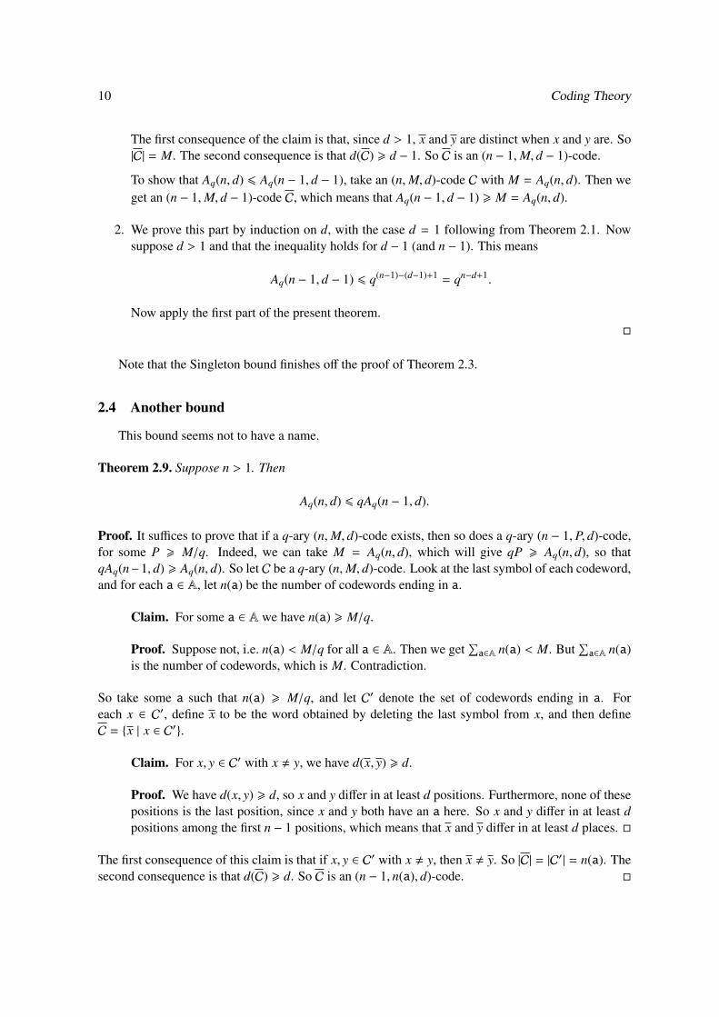
The first consequence of the claim is that, since d > 1, x and y are distinct when x and y are. So|C| = M. The second consequence is that d(C) > d − 1. So C is an (n − 1,M, d − 1)-code.
To show that Aq(n, d) 6 Aq(n − 1, d − 1), take an (n,M, d)-code C with M = Aq(n, d). Then weget an (n − 1,M, d − 1)-code C, which means that Aq(n − 1, d − 1) > M = Aq(n, d).
2. We prove this part by induction on d, with the case d = 1 following from Theorem 2.1. Nowsuppose d > 1 and that the inequality holds for d − 1 (and n − 1). This means
Aq(n − 1, d − 1) 6 q(n−1)−(d−1)+1 = qn−d+1.
Now apply the first part of the present theorem.�
Note that the Singleton bound finishes off the proof of Theorem 2.3.
2.4 Another bound
This bound seems not to have a name.
Theorem 2.9. Suppose n > 1. Then
Aq(n, d) 6 qAq(n − 1, d).
Proof. It suffices to prove that if a q-ary (n,M, d)-code exists, then so does a q-ary (n − 1, P, d)-code,for some P > M/q. Indeed, we can take M = Aq(n, d), which will give qP > Aq(n, d), so thatqAq(n−1, d) > Aq(n, d). So let C be a q-ary (n,M, d)-code. Look at the last symbol of each codeword,and for each a ∈ A, let n(a) be the number of codewords ending in a.
Claim. For some a ∈ A we have n(a) > M/q.
Proof. Suppose not, i.e. n(a) < M/q for all a ∈ A. Then we get∑a∈A n(a) < M. But
∑a∈A n(a)
is the number of codewords, which is M. Contradiction.
So take some a such that n(a) > M/q, and let C′ denote the set of codewords ending in a. Foreach x ∈ C′, define x to be the word obtained by deleting the last symbol from x, and then defineC = {x | x ∈ C′}.
Claim. For x, y ∈ C′ with x , y, we have d(x, y) > d.
Proof. We have d(x, y) > d, so x and y differ in at least d positions. Furthermore, none of thesepositions is the last position, since x and y both have an a here. So x and y differ in at least dpositions among the first n − 1 positions, which means that x and y differ in at least d places. �
The first consequence of this claim is that if x, y ∈ C′ with x , y, then x , y. So |C| = |C′| = n(a). Thesecond consequence is that d(C) > d. So C is an (n − 1, n(a), d)-code. �

Good codes 11
2.5 The Plotkin bound
The Plotkin bound is more complicated, but more useful. There is a version for arbitrary q, butwe’ll address only binary codes. First, we prove some elementary inequalities that we shall need later.
Lemma 2.10. Suppose N,M are integers with 0 6 N 6 M. Then
N(M − N) 6
M2
4(if M is even)
M2 − 14
(if M is odd).
Proof. The graph of N(M − N) is an unhappy quadratic with its turning point at N = M/2, so tomaximise it we want to make N as near as possible to this (remembering that N must be an integer).If M is even, then we can take N = M/2, while if M is odd we take N = (M − 1)/2. �
Now we need to recall some notation: remember that if x ∈ R, then bxc is the largest integer whichis less than or equal to x.
Lemma 2.11. If x ∈ R, then b2xc 6 2bxc + 1.
Proof. Let y = bxc; then x < y + 1. So 2x < 2y + 2, so b2xc 6 2y + 1. �
Now we can state the Plotkin bound – there are two cases, depending on whether d is even or odd.But in fact either one of these can be recovered from the other, using Theorem 2.3.
Theorem 2.12 (Plotkin bound).
1. If d is even and n < 2d, then
A2(n, d) 6 2⌊
d2d − n
⌋.
2. If d is odd and n < 2d + 1, then
A2(n, d) 6 2⌊
d + 12d + 1 − n
⌋.
The proof is a double-counting argument. Suppose C is a binary (n,M, d)-code. We suppose thatour alphabet is {0, 1}, and if v = (v1 . . . vn) and w = (w1 . . .wn) are codewords, then we define v +w tobe the word (v1 + w1)(v2 + w2) . . . (vn + wn), where we do addition modulo 2 (so 1 + 1 = 0).
A really useful feature of this addition operation is the following.
Lemma 2.13. Suppose v, are binary words of length n. Then d(v,w) is the number of 1s in v + w.
Proof. By looking at the possibilities for vi and wi, we see that
(v + w)i =
0 (if vi = wi)1 (if vi , wi)
.
So
d(v,w) = |{i | vi , wi}|
= |{i | (v + w)i = 1}|.

12 Coding Theory
�
Now we write down an(
M2
)by n array A whose rows are all the words v + w for pairs of distinct
codewords v,w. We’re going to count the number of 1s in this array in two different ways.
Lemma 2.14. The number of 1s in A is at mostn
M2
4(if M is even)
nM2 − 1
4(if M is odd)
.
Proof. We count the number of 1s in each column. The word v + w has a 1 in the jth position if andonly if one of v and w has a 1 in the jth position, and the other has a 0. If we let N be the number ofcodewords which have a 1 in the jth position, then the number ways of choosing a pair v,w such thatv + w has a 1 in the jth position is N(M − N). So the number of 1s in the jth column of our array is
N(M − N) 6
M2
4(if M is even)
M2 − 14
(if M is odd)
by Lemma 2.10. This is true for every j, so by adding up we obtain the desired inequality. �
Now we count the 1s in A in a different way.
Lemma 2.15. The number of 1s in A is at least d(
M2
).
Proof. We look at the number of 1s in each row. The key observation is that if v,w are codewords,then the number of 1s in v + w is d(v,w), and this is at least d. So there are at least d 1s in each row,and hence at least d
(M2
)altogether. �
Proof of the Plotkin bound. We assume first that d is even. Suppose we have a binary (n,M, d)-codeC, and construct the array as above. Now we simply combine the inequalities of Lemma 2.14 andLemma 2.15. There are two cases, according to whether M is even or odd.
Case 1: M even By combining the two inequalities, we get
d(M2
)6 n
M2
4
⇒dM2
2−
dM26
nM2
4⇒ (2d − n)M2 6 2dM.
By assumption, 2d − n and M are both positive, so we divide both sides by (2d − n)M to get
M 62d
2d − n.
But M is an integer, so in fact
M 6⌊
2d2d − n
⌋6 2
⌊d
2d − n
⌋+ 1;
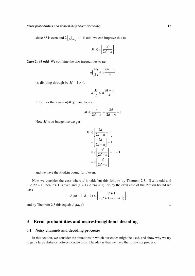
Error probabilities and nearest-neighbour decoding 13
since M is even and 2⌊
d2d−n
⌋+ 1 is odd, we can improve this to
M 6 2⌊
d2d − n
⌋.
Case 2: M odd We combine the two inequalities to get
d(M2
)6 n
M2 − 14,
or, dividing through by M − 1 > 0,
dM26 n
M + 14.
It follows that (2d − n)M ≤ n and hence
M 6n
2d − n=
2d2d − n
− 1.
Now M is an integer, so we get
M 6⌊
2d2d − n
− 1⌋
=
⌊2d
2d − n
⌋− 1
6 2⌊
d2d − n
⌋+ 1 − 1
= 2⌊
d2d − n
⌋,
and we have the Plotkin bound for d even.
Now we consider the case where d is odd; but this follows by Theorem 2.3. If d is odd andn < 2d + 1, then d + 1 is even and (n + 1) < 2(d + 1). So by the even case of the Plotkin bound wehave
A2(n + 1, d + 1) 6⌊
(d + 1)2(d + 1) − (n + 1)
⌋,
and by Theorem 2.3 this equals A2(n, d). �
3 Error probabilities and nearest-neighbour decoding
3.1 Noisy channels and decoding processes
In this section, we consider the situations in which our codes might be used, and show why we tryto get a large distance between codewords. The idea is that we have the following process.

14 Coding Theory
codeword
Noisy channely
distorted word
Decoding processy
codeword
We’d like the codeword at the bottom to be the same as the codeword at the top as often as possible.This relies on a good choice of code, and a good choice of decoding process. Most of this course isdevoted to looking at good codes, but here we look at decoding processes. Given a code C of lengthn over the alphabet A, a decoding process is simply a function from An to C – given a received word,we try to ‘guess’ which word was sent.
We make certain assumptions about our noisy channel, namely that all errors are independent andequally likely. This means that there is some error probability p such that any transmitted symbol awill be transmitted correctly with probability 1 − p, or incorrectly with probability p, and that if thereis an error then all the incorrect symbols are equally likely. Moreover, errors on different symbols areindependent – whether an error occurs in one symbol has no effect on whether errors occur in latersymbols. We also assume that p 6 1
2 .Suppose we have a decoding process f : An → C. We say that f is a nearest-neighbour decoding
process if for all w ∈ An and all v ∈ C we have
d(w, f (w)) 6 d(w, v).
This means that for any received word, we decode it using the nearest codeword. Note that some code-words may be equally near, so there may be several different nearest-neighbour decoding processesfor a given code.
Example. Let C be the binary repetition code of length 5:
{00000, 11111}.
Let f be the decoding process
w 7→
00000 (if w contains at least three 0s)11111 (if w contains at least three 1s)
.
Then f is the unique nearest-neighbour decoding process for C.
Given a code and a decoding process, we consider the word error probability: given a codeword w,what is the probability that after distortion and decoding, we end up with a different codeword? Let’scalculate this for the above example, with w = 00000. It’s clear that this will be decoded wrongly ifat least three of the symbols are changed into 1s. If the error probability of the channel is p, then theprobability that this happens is
p3(1 − p)2(53
)+ p4(1 − p)
(54
)+ p5
(55
)= 6p5 − 15p4 + 10p3.
For example, if p = 14 , then the word error probability is only about 0.104.

Linear codes 15
In general, word error probability depends on the particular word, and we seek a decoding processwhich minimises the maximum word error probability. It can be shown that the best decoding processin this respect is always a nearest-neighbour decoding process (remembering our assumption thatp 6 1
2 ).
3.2 Rates of transmission and Shannon’s Theorem
Given a q-ary (n,M, d)-code C, we define the rate of C to be
logq M
n;
this can be interpreted as the ratio of ‘useful information’ to ‘total information’ transmitted. Forexample, the q-ary repetition code of length 3 is a (3, q, 3)-code, so has rate 1
3 . The useful informationin a codeword can be thought of as the first digit – the rest of the digits are just redundant informationincluded to reduce error probabilities.
Clearly, its good to have a code with a high rate. On the other hand, it’s good to have codeswith low word error probabilities. Shannon’s Theorem says that these two aims can be achievedsimultaneously, as long as we use a long enough code. We’ll restrict attention to binary codes. Weneed to define the capacity of our noisy channel – if the channel has error probability p, then thecapacity is
C(p) = 1 + p log2 p + (1 − p) log2(1 − p).
Theorem 3.1 (Shannon’s Theorem). Suppose we have a noisy channel with capacity C. Suppose εand ρ are positive real numbers with ρ < C. Then for any sufficiently large n, there exists a binarycode of length n and rate at least ρ and a decoding process such that the word error probability is atmost ε.
What does the theorem say? It says that as long as the rate of our code is less than the capacity ofthe channel, we can make the word error probability as small as we like. The proof of this theorem iswell beyond the scope of this course.
Note that if p = 12 , then C(p) = 0. This reflects the fact that it is hopeless transmitting through
such a channel – given a received word, the codeword sent is equally likely to be any codeword.
4 Linear codes
For the rest of the course, we shall be restricting our attention to linear codes; these are codes inwhich the alphabet A is a finite field, and the code itself forms a vector space over A. These codes areof great interest because:
• they are easy to describe – we need only specify a basis for our code;
• it is easy to calculate the minimum distance of a linear code – we need only calculate thedistance of each word from the word 00 . . . 0;
• it is easy to decode an error-correcting linear code, via syndrome decoding;
• many of the best codes known are linear; in particular, every known non-trivial perfect code hasthe same parameters (i.e. length, number of codewords and minimum distance) as some linearcode.

16 Coding Theory
4.1 Revision of linear algebra
Recall from Linear Algebra the definition of a field: a set F with distinguished elements 0 and 1and binary operations + and × such that:
• F forms an abelian group under +, with identity element 0 (that is, we have
� a + b = b + a,
� (a + b) + c = a + (b + c),
� a + 0 = a,
� there exists an element −a of F such that −a + a = 0
for all a, b, c ∈ F);
• F \ {0} forms an abelian group under ×, with identity element 1 (that is, we have
� a × b = b × a,
� (a × b) × c = a × (b × c),
� a × 1 = a,
� there exists an element a−1 of F such that a−1 × a = 1
for all a, b, c ∈ F \ {0});
• a × (b + c) = (a × b) + (a × c) for all a, b, c ∈ F.
We make all the familiar notational conventions: we may write a×b as a.b or ab; we write a×b−1
as a/b; we write a + (−b) as a − b.We shall need the following familiar property of fields.
Lemma 4.1. Let F be a field, and a, b ∈ F. Then ab = 0 if and only if a = 0 or b = 0.
We also need to recall the definition of a vector space. If F is a field, then a vector space over F isa set V with a distinguished element 0, a binary operation + and a function × : (F × V) → V (that is,a function which, given an element λ of F and an element v of V , produces a new element λ × v of V)such that:
• V is an abelian group under + with identity 0;
• for all λ, µ ∈ F and u, v ∈ V , we have
� (λ × µ) × v = λ × (µ × v),
� (λ + µ) × v = (λ × v) + (µ × v),
� λ × (u + v) = (λ × u) + (λ × v),
� 1 × v = v.
There shouldn’t be any confusion between the element 0 of F and the element 0 of V , or betweenthe different versions of + and ×. We use similar notational conventions for + and × those that we usefor fields.
If V is a vector space over F, then a subspace is a subset of V which is also a vector space underthe same operations. In fact, a subset W of V is a subspace if and only if

Linear codes 17
• 0 ∈ W,
• v + w ∈ W, and
• λv ∈ W
whenever v,w ∈ W and λ ∈ F.Suppose V is a vector space over F and v1, . . . , vn ∈ V . Then we say that v1, . . . , vn are linearly
independent if there do not not exist λ1, . . . , λn ∈ F which are not all zero such that
λ1v1 + · · · + λnvn = 0.
We define the span of v1, . . . , vn to be the set of all linear combinations of v1, . . . , vn, i.e. the set
〈v1, . . . , vn〉 = {λ1v1 + · · · + λnvn | λ1, . . . , λn ∈ F}.
The span of v1, . . . , vn is always a subspace of V . If it the whole of V , we say that v1, . . . , vn span V .We say that V is finite-dimensional if there is a finite set v1, . . . , vn that spans V . A set v1, . . . , vn
which is linearly independent and spans V is called a basis for V . If V is finite-dimensional, then ithas at least one basis, and all bases of V have the same size. This is called the dimension of V , whichwe write as dim(V).
Suppose V,W are vector spaces over F. A linear map from V to W is a function α : V → W suchthat
α(λu + µv) = λα(u) + µα(v)
for all λ, µ ∈ F and u, v ∈ V . If α is a linear map, the kernel of α is the subset
ker(α) = {v ∈ V | α(v) = 0}
of V , and the image of α is the subset
Im(α) = {α(v) | v ∈ V}
of W. ker(α) is a subspace of V , and we refer to its dimension as the nullity of α, which we write n(α).Im(α) is a subspace of W, and we refer to its dimension as the rank of α, which we write r(α). TheRank–nullity Theorem says that if α is a linear map from V to W, then
n(α) + r(α) = dim(V).
We shall only be interested in one particular type of vector space. For a non-negative integer n, weconsider the set Fn, which we think of as the set of column vectors of length n over F, with operations
x1...
xn
+
y1...
yn
=
x1 + y1...
xn + yn
and
λ
x1...
xn
=λx1...
λxn
.

18 Coding Theory
Fn is a vector space over F of dimension n. Sometimes we will think of the elements of Fn as rowvectors rather than column vectors, or as words of length n over F.
Given m, n and an n × m matrix A over F, we can define a linear map Fm → Fn bya11 . . . a1m...
...
an1 . . . anm
x1...
xm
=
a11x1 + · · · + a1mxm...
an1x1 + · · · + anmxm
.Every linear map from Fm to Fn arises in this way. The rank of A is defined to be the rank of this linearmap. The column rank of A is defined to be the dimension of 〈c1, . . . , cm〉, where c1, . . . , cm are thecolumns of A regarded as vectors in Fn, and the row rank is defined to be the dimension of 〈r1, . . . , rn〉,where r1, . . . , rn are the rows of A regarded as (row) vectors in Fm. We shall need the result that therank, row rank and column rank of A are all equal.
Note that when we think of Fn as the space of row vectors rather than column vectors, we maythink of a linear map as being multiplication on the right by an m × n matrix.
4.2 Finite fields and linear codes
The examples of fields you are most familiar with are Q, R and C. But these are of no interest inthis course – we are concerned with finite fields. The classification of finite fields goes back to Galois.
Theorem 4.2. Let q be an integer greater than 1. Then a field of order q exists if and only if q is aprime power, and all fields of order q are isomorphic.
If q is a prime power, then we refer to the unique field of order q as Fq. For example, if q isactually a prime, then Fq simply consists of the integers mod q, with the operations of addition andmultiplication mod q. It is a reasonably easy exercise to show that this really is a field – the hardpart is to show that multiplicative inverses exist, and this is a consequence of the Chinese RemainderTheorem.
If q is a prime power but not a prime, then the field Fq is awkward to describe without developinglots of theory. But this need not worry us – all the explicit examples we meet will be over fieldsof prime order. Just remember that there is a field of each prime power order. As an example, theaddition and multiplication tables for the field of order 4 are given below; we write F4 = {0, 1, a, b}.
+ 0 1 a b0 0 1 a b1 1 0 b aa a b 0 1b b a 1 0
× 0 1 a b0 0 0 0 01 0 1 a ba 0 a b 1b 0 b 1 a
What this means for coding theory is that if we have a q-ary alphabet A with q a prime power,then we may assume that A = Fq (since A is just a set of size q with no additional structure, we losenothing by re-labelling the elements of A as the elements of Fq) and we gets lots of extra structure onA (i.e. the structure of a field) and on An = Fn
q (the structure of a vector space).
Definition. Assume that q is a prime power and that A = Fq. A linear code over A is a subspace ofAn.

Linear codes 19
Example. The binary (5, 4, 3)-code
{00000, 01101, 10110, 11011}
that we saw earlier is linear. To check this, we have to show that it is closed under addition and scalarmultiplication. Scalar multiplication is easy: the only elements of F2 are 0 and 1, and we have
0x = 00000, 1x = x
for any codeword x. For addition, notice that we have x + x = 00000 and x + 00000 = x for any x,and
01101 + 10110 = 11011,
01101 + 11011 = 10110,
10110 + 11011 = 10110.
4.3 The minimum distance of a linear code
One of the advantages of linear codes that we mentioned earlier is that it’s easy to find the mini-mum distance of a linear code. Given a code C and a codeword x, we define the weight weight(x) ofx to be the number of non-zero symbols in x.
Lemma 4.3. Suppose x, y and z are codewords in a linear code over Fq, and λ is a non-zero elementof Fq. Then:
1. d(x + z, y + z) = d(x, y);
2. d(λx, λy) = d(x, y);
3. d(x, y) = weight(x − y).
Proof. We write x = x1 . . . xn, y = y1 . . . yn, z = z1 . . . zn.
1. The ith symbol of x + z is xi + zi, and the ith symbol of y + z is yi + zi. So we have
d(x + z, y + z) = |{i | xi + zi , yi + zi}.
Now for any xi, yi, zi we have xi + zi , yi + zi if and only if xi , yi (since we can just add orsubtract zi to/from both sides). So
d(x + z, y + z) = {i | xi , yi}
= d(x, y).
2. The ith symbol of λx is λxi, and the ith symbol of λy is λyi, so
d(λx, λy) = |{i | λxi , λyi}.
Now since λ , 0 we have λxi , λyi if and only if xi , yi (since we can multiply both sides byλ or λ−1). So we find
d(λx, λy) = |{i | xi , yi}|
= d(x, y).

20 Coding Theory
3. Clearly weight(x − y) = d(x − y, 0), which equals d(x, y) by part (1).
�
Corollary 4.4. The minimum distance of a linear code C equals the minimum weight of a non-zerocodeword in C.
Proof. It suffices to show that, for any δ,
(C contains distinct codewords x, y with d(x, y) = δ)⇔ (C contains a non-zero codeword x with weight(x) = δ).
(⇐) Cmust contain the zero element of Fnq, namely the word 00 . . . 0. This is because Cmust contain
some word x, and hence must contain 0x = 00 . . . 0. So if x is a non-zero codeword with weightδ, then x and 00 . . . 0 are distinct codewords with d(w, 00 . . . 0) = δ.
(⇒) If x, y are distinct codewords with d(x, y) = δ, then x− y is a non-zero codeword with weight(x−y) = δ.
�
4.4 Bases and generator matrices
Another advantage of linear codes that I mentioned above is that you can specify the whole codeby specifying a basis. Recall that a basis of a vector space V over F is a subset {e1, . . . , ek} such thatevery v ∈ V can be uniquely written in the form
v = λ1e1 + λ2e2 + · · · + λkek,
where λ1, . . . , λk are elements of F.Any two bases have the same size, and this size is called the dimension of the code.
Example. The set {01101, 11011} is a basis for the code in the last example.
In general, V will have lots of different bases to choose from. But (recall from Linear Algebra)that any two bases have the same size, and this size we call the dimension of V . So the code in theexamples above has dimension 2. If a code C is of length n and has dimension k as a vector space, wesay that C is an [n, k]-code. If in addition C has minimum distance at least d, we may say that C is an[n, k, d]-code. So the code in the example above is a binary [5, 2, 3]-code.
Lemma 4.5. A vector space V of dimension k over Fq contains exactly qk elements.
Proof. Suppose {e1, . . . , ek} is a basis for V . Then, by the definition of a basis, every element of V isuniquely of the form
λ1e1 + λ2e2 + · · · + λkek,
for some choice of λ1, . . . , λk ∈ Fq. On the other hand, every choice of λ1, . . . , λk gives us an elementof V , so the number of vectors in V is the number of choices of λ1, . . . , λk. Now there are q ways tochoose each λi (since there are q elements of Fq to choose from), and so the total number of choicesof these scalars is qk. �

Linear codes 21
As a consequence, we see that a q-ary [n, k, d]-code is a q-ary (n, qk, d)-code. This highlights aslight disadvantage of linear codes – their sizes must be powers of q. So if we’re trying to find optimalcodes for given values of n, d (i.e. (n,M, d)-codes with M = Aq(n, d)), then we can’t hope to do thiswith linear codes if Aq(n, d) is not a power of q. In practice (especially for q = 2) many of the valuesof Aq(n, d) are powers of q.
It will be useful in the rest of the course to arrange a basis of our code in the form of a matrix.
Definition. Suppose C is a q-ary [n, k]-code. A generator matrix for C is a k × n matrix with entriesin Fq, whose rows form a basis for C.
Examples.1. The binary [5, 2, 3]-code from the last example has various different generator matrices; for
example (01101
10110
),
(10110
11011
).
2. If q is a prime power, then the q-ary repetition code is linear. It has a generator matrix
(11 . . . 1).
3. Recall the binary parity-check code
C = {v = v1v2 . . . vn | v1, . . . , vn ∈ F2, v1 + · · · + vn = 0}.
This has a generator matrix
1 0 . . . 0 0 1
0 1 . . . 0 0 1....... . .
...... 1
0 0 . . . 1 0 1
0 0 . . . 0 1 1
.
4.5 Equivalence of linear codes
Recall the definition of equivalent codes from earlier: C is equivalent to D if we can get from CtoD via a sequence of operations of the following two types.
Operation 1: permuting positions Choose a permutation σ of {1, . . . , n}, and for v = v1 . . . vn ∈ An
definevσ = vσ(1) . . . vσ(n).
Now replace C withCσ = {vσ | v ∈ C}.
Operation 2: permuting the symbols in a given position Choose i ∈ {1, . . . , n} and a permutationf of A. Forv = v1 . . . vn ∈ An, define
v f ,i = v1 . . . vi−1( f (vi))vi+1 . . . vn.
Now replace C withC f ,i = {v f ,i | v ∈ C}.

22 Coding Theory
There’s a slight problem with applying this to linear codes, which is that if C is linear and D isequivalent to C, thenD need not be linear. Operation 1 is OK, as we shall now show.
Lemma 4.6. Suppose C is a linear [n, k, d]-code over Fq, and σ is a permutation of {1, . . . , n}. Thenthe map
φ : C −→ Fnq
v 7−→ vσ
is linear, and Cσ is a linear [n, k, d]-code.
Proof. Suppose v,w ∈ C and λ, µ ∈ Fq. We need to show that
φ(λv + µw) = λφ(v) + µφ(w),
i.e.(φ(λv + µw))i = (λφ(v) + µφ(w))i
for every i ∈ {1, . . . , n}. We have
(φ(λv + µw))i = ((λv + µw)σ)i
= (λv + µw)σ(i)
= (λv)σ(i) + (µw)σ(i)
= λ(vσ(i)) + µ(wσ(i))
= λ(vσ)i + µ(wσ)i
= λ(φ(v))i + µ(φ(w))i
= (λφ(v))i + (µφ(w))i
= (λφ(v) + µφ(w))i,
as required.Now Cσ is by definition the image of φ, and so is a subspace of Fn
q, i.e. a linear code. We knowthat d(Cσ) = d(C) from before, and that |Cσ| = |C|. This implies qdimCσ = qdimC by Lemma 4.5, i.e.dimCσ = dimC = k, so Cσ is an [n, k, d]-code. �
Unfortunately, Operation 2 does not preserve linearity. Here is a trivial example of this. Supposeq = 2, n = 1 and C = {0}. Then C is a linear [1, 0]-code. If we choose i = 1 and f the permutationwhich swaps 0 and 1, then we have C f ,i = {1}, which is not linear. So we need to restrict Operation 2.We define the following.
Operation 2′ Suppose C is a linear code of length n over Fq. Choose i ∈ {1, . . . , n} and a ∈ Fq \ {0}.For v = v1 . . . vn ∈ F
nq define
va,i = v1 . . . vi−1(avi)vi+1 . . . vn.
Now replace C with the codeCa,i = {va,i | v ∈ C}.

Linear codes 23
We want to show that Operation 2′ preserves linearity, dimension and minimum distance. We beingby showing that it’s a special case of Operation 2.
Lemma 4.7. If a ∈ Fq \ {0}, the the map
f : Fq −→ Fq
x 7−→ ax
is a bijection, i.e. a permutation of Fq.
Proof. Since f is a function from a finite set to itself, we need only show that f is injective. If x, y ∈ Fq
and f (x) = f (y), then we have ax = ay. Since a , {0}, a has an inverse a−1, and we can multiply bothsides by a−1 to get x = y. So f is injective. �
Now we show that the operation which sends v to va,i is linear, which will mean that it sends linearcodes to linear codes.
Lemma 4.8. Suppose C is a linear [n, k, d]-code over Fq, i ∈ {1, . . . , n} and 0 , a ∈ Fq. Then the map
φ : Fnq −→ F
nq
v 7−→ va,i
is linear, and Ca,i is a linear [n, k, d]-code over Fq.
Proof. For any vector v ∈ Fnq, we have
φ(v) j = (va,i) j =
av j ( j = i)v j ( j , i)
.
Now take v,w ∈ Fnq and λ, µ ∈ Fq. We must show that
(φ(λv + µw)) j = (λφ(v) + µφ(w)) j
for each j ∈ {1, . . . , n}. For j , i we have
(φ(λv + µw)) j = (λv + µw) j
= (λv) j + (µw) j
= λv j + µw j
= λ(φ(v)) j + µ(φ(w)) j
= (λφ(v)) j + (µφ(w)) j,
= (λφ(v) + µφ(w)) j,
while for j = i we have
(φ(λv + µw)) j = a(λv + µw) j
= a((λv) j + (µw) j)
= a(λv j + µw j)
= aλv j + aµw j
= λ(av j) + µ(aw j)
= λ(φ(v) j) + µ(φ(w) j)
= (λφ(v)) j + (µφ(w)) j
= (λφ(v) + µφ(w)) j,

24 Coding Theory
as required.Now Ca,i is by definition the image of φ, and this is a subspace of Fn
q, i.e. a linear code. We knowfrom before (since Operation 2′ is a special case of Operation 2) that d(Ca,i) = d(C) and |Ca,i| = |C|,and this gives dimCa,i = dimC = k, so that Ca,i is a linear [n, k, d]-code. �
In view of these results we re-define equivalence for linear codes: we say that linear codes C andD are equivalent if we can get from one to the other by applying Operations 1 and 2′ repeatedly.
Example. Let n = q = 3, and define
C = {000, 101, 202},
D = {000, 011, 022},
E = {000, 012, 021}.
Then C, D and E are all [3, 1]-codes over Fq (check this!). We can get from C to D by swapping thefirst two positions, and we can get from D to E by multiplying everything in the third position by 2.So C,D and E are equivalent linear codes.
We’d like to know the relationship between equivalence and generator matrices: if C and D areequivalent linear codes, how are their generator matrices related? Well, a given code usually hasmore than one choice of generator matrix, and so first we’d like to know how two different generatormatrices for the same code are related.
We define the following operations on matrices over Fq:
MO1. permuting the rows;
MO2. multiplying a row by a non-zero element of Fq;
MO3. adding a multiple of a row to another row.
You should recognise these as the ‘elementary row operations’ from Linear Algebra. Their im-portance is as follows.
Lemma 4.9. Suppose C is a linear [n, k]-code with generator matrix G. If the matrix H can beobtained from G by applying the row operations (MO1–3) repeatedly, then H is also a generatormatrix for C.
Proof. Since G is a generator matrix for C, we know that the rows of G are linearly independent andspan C. So G has rank k (the number of rows) and row space C. We know from linear algebra thatelementary row operations do not affect the rank or the row space of a matrix, so H also has rank kand row space C. So the rows of H are linearly independent and span C, so form a basis for C, i.e. His a generator matrix for C. �
Now we define two more matrix operations:
MO4. permuting the columns;
MO5. multiplying a column by a non-zero element of Fq.
Lemma 4.10. Suppose C is a linear [n, k]-code over Fq, with generator matrix G. If the matrix His obtained from G by applying matrix operation 4 or 5, then H is a generator matrix for a code Dequivalent to C.

Linear codes 25
Proof. Suppose G has entries g jl, for 1 6 j 6 k and 1 6 l 6 n. Let r1, . . . , rk be the rows of G, i.e.
r j = g j1g j2 . . . g jn.
By assumption {r1, . . . , rk} is a basis for C; in particular, the rank of G is k.Suppose H is obtained using matrix operation 4, applying a permutation σ to the columns. This
means thath jl = g jσ(l),
so row j of H is the wordg jσ(1)g jσ(2) . . . g jσ(n).
But this is the word (r j)σ as defined in equivalence operation 1. So the rows of H lie in the code Cσ,which is equivalent to C.
Now suppose instead that we obtain H by applying matrix operation 5, multiplying column i bya ∈ Fq \ {0}. This means that
h jl =
g jl (l , i)ag jl (l = i)
,
so that row j of H is the word
g j1g j2 . . . g j(i−1)(ag ji)g j(i+1) . . . g jn.
But this is the word (r j)a,i as defined in equivalence operation 2. So the rows of H lie in the code Ca,i,which is equivalent to C.
For either matrix operation, we have seen that the rows of H lie in a code D equivalent to C. Weneed to know that they form a basis for D. Since there are k rows and dim(D) = dim(C) = k, itsuffices to show that the rows of H are linearly independent, i.e. to show that H has rank k. But matrixoperations 4 and 5 are elementary column operation, and we know from linear algebra that these don’taffect the rank of a matrix. So rank(H) = rank(G) = k. �
We can summarise these results as follows.
Proposition 4.11. Suppose C is a linear [n, k]-code with a generator matrix G, and that the matrix His obtained by applying a sequence of matrix operations 1–5. Then H is a generator matrix for a codeD equivalent to C.
Proof. By applying matrix operations 1–3, we get a new generator matrix for C, by Lemma 4.9, andC is certainly equivalent to itself. By applying matrix operations 4 and 5, we get a generator matrixfor a code equivalent to C, by Lemma 4.10. �
Note that in the list of matrix operations 1–5, there is a sort of symmetry between rows andcolumns. In fact, you might expect that you can do another operation
MO6. adding a multiple of a column to another column
but you can’t. Doing this can take you to a code with a different minimum distance. For example,suppose q = 2, and that C is the parity-check code of length 3:
C = {000, 011, 101, 110}.
26 Coding Theory
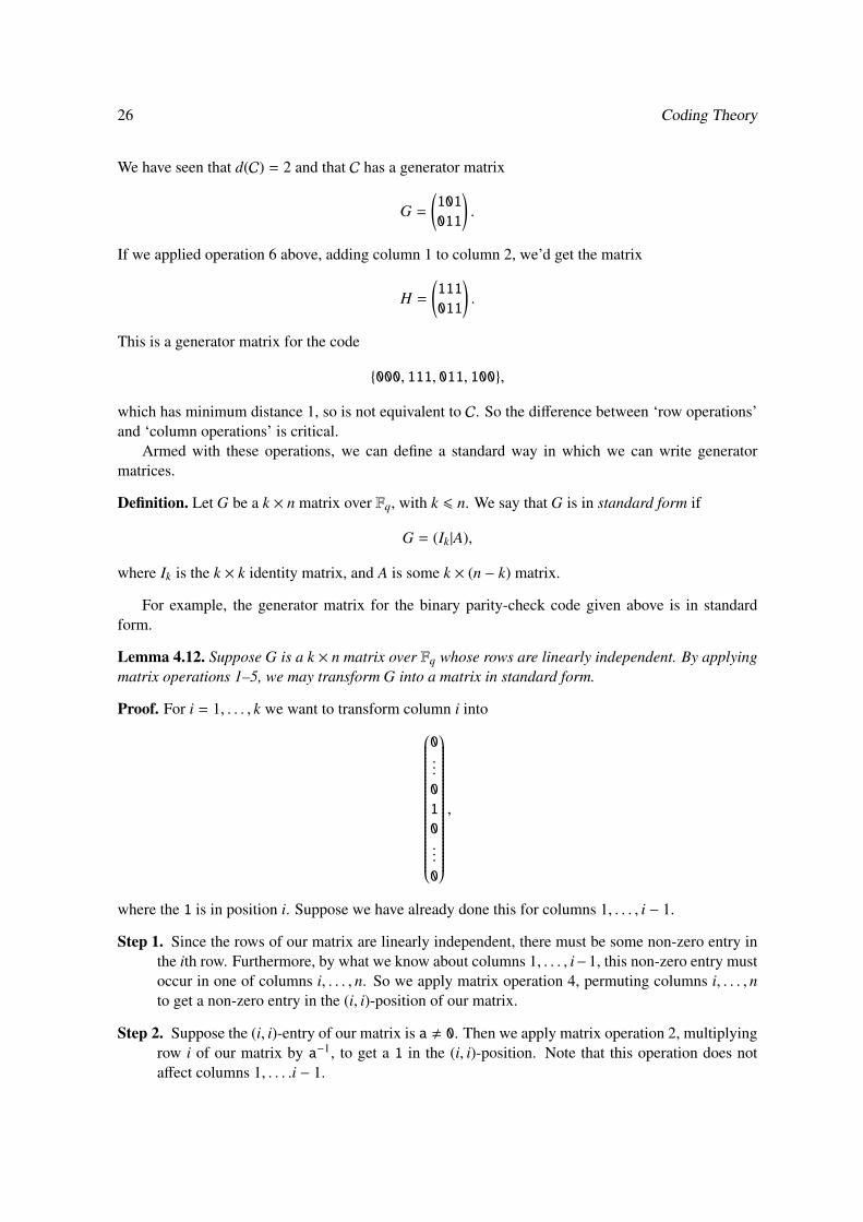
We have seen that d(C) = 2 and that C has a generator matrix
G =(101
011
).
If we applied operation 6 above, adding column 1 to column 2, we’d get the matrix
H =(111
011
).
This is a generator matrix for the code
{000, 111, 011, 100},
which has minimum distance 1, so is not equivalent to C. So the difference between ‘row operations’and ‘column operations’ is critical.
Armed with these operations, we can define a standard way in which we can write generatormatrices.
Definition. Let G be a k × n matrix over Fq, with k 6 n. We say that G is in standard form if
G = (Ik|A),
where Ik is the k × k identity matrix, and A is some k × (n − k) matrix.
For example, the generator matrix for the binary parity-check code given above is in standardform.
Lemma 4.12. Suppose G is a k × n matrix over Fq whose rows are linearly independent. By applyingmatrix operations 1–5, we may transform G into a matrix in standard form.
Proof. For i = 1, . . . , k we want to transform column i into
0...
0
1
0...
0
,
where the 1 is in position i. Suppose we have already done this for columns 1, . . . , i − 1.
Step 1. Since the rows of our matrix are linearly independent, there must be some non-zero entry inthe ith row. Furthermore, by what we know about columns 1, . . . , i−1, this non-zero entry mustoccur in one of columns i, . . . , n. So we apply matrix operation 4, permuting columns i, . . . , nto get a non-zero entry in the (i, i)-position of our matrix.
Step 2. Suppose the (i, i)-entry of our matrix is a , 0. Then we apply matrix operation 2, multiplyingrow i of our matrix by a−1, to get a 1 in the (i, i)-position. Note that this operation does notaffect columns 1, . . . .i − 1.

Linear codes 27
Step 3. We now apply matrix operation 3, adding multiples of row i to the other rows in order to ‘kill’the remaining non-zero entries in column i. Note that this operation does not affect columns1, . . . .i − 1.
By applying Steps 1–3 for i = 1, . . . , k in turn, we get a matrix in standard form. Note that it is auto-matic from the proof that k 6 n. �
Corollary 4.13. Suppose C is a linear [n, k]-code over Fq. Then C is equivalent to a code with agenerator matrix in standard form.
Proof. G has linearly independent rows, so by Lemma 4.12 we can transform G into a matrix H instandard form using matrix operations 1–5. By Proposition 4.11, H is a generator matrix for a codeequivalent to C. �
4.6 Decoding with a linear code
Recall the notion of a nearest-neighbour decoding process from §3. For linear codes, we can findnearest-neighbour decoding processes in an efficient way, using cosets.
Definition. Suppose C is an [n, k]-code over Fq. For v ∈ Fnq, define
v + C = {v + w | w ∈ C}.
The set v + C is a called a coset of C.
You should remember the word coset from group theory, and this is exactly what cosets are here– cosets of the group C as a subgroup of Fn
q.
Example. Let q = 3, and consider the [2, 1]-code
C = {00, 12, 21}.
The cosets of C are00 + C = {00, 12, 21},
11 + C = {11, 20, 02},
22 + C = {22, 01, 10}.
The crucial property of cosets is as follows.
Proposition 4.14. Suppose C is an [n, k]-code over Fq. Then:
1. every coset of C contains exactly qk words;
2. every word in Fnq is contained in some coset of C;
3. if the word v is contained in the coset u + C, then v + C = u + C;
4. any word in Fnq is contained in at most one coset of C;
5. there are exactly qn−k cosets of C.
28 Coding Theory
Proof.1. C contains qk words, and the map from C to v + C given by w 7→ v + w is a bijection.
2. The word v is contained in v + C, since v = 0 + v and 0 ∈ C.
3. Since v ∈ u+C, we have v = u+ x for some x ∈ C. If w ∈ v+C, then w = v+ y for some y ∈ C,so w = u + (x + y) ∈ u + C. So v + C is a subset of u + C; since they both have the same size,they must be equal.
4. Suppose u ∈ v + C and u ∈ w + C. Then we have u = v + x and u = w + y for some x, y ∈ C.Since C is closed under addition, we have y − x ∈ C, so we find that v = w + (y − x) ∈ w + C.Hence v + C = w + C by part (3).
5. There are qn words altogether in Fnq, and each of them is contained in exactly one coset of C.
Each coset has size qk, and so the number of cosets must be qn/qk = qn−k.�
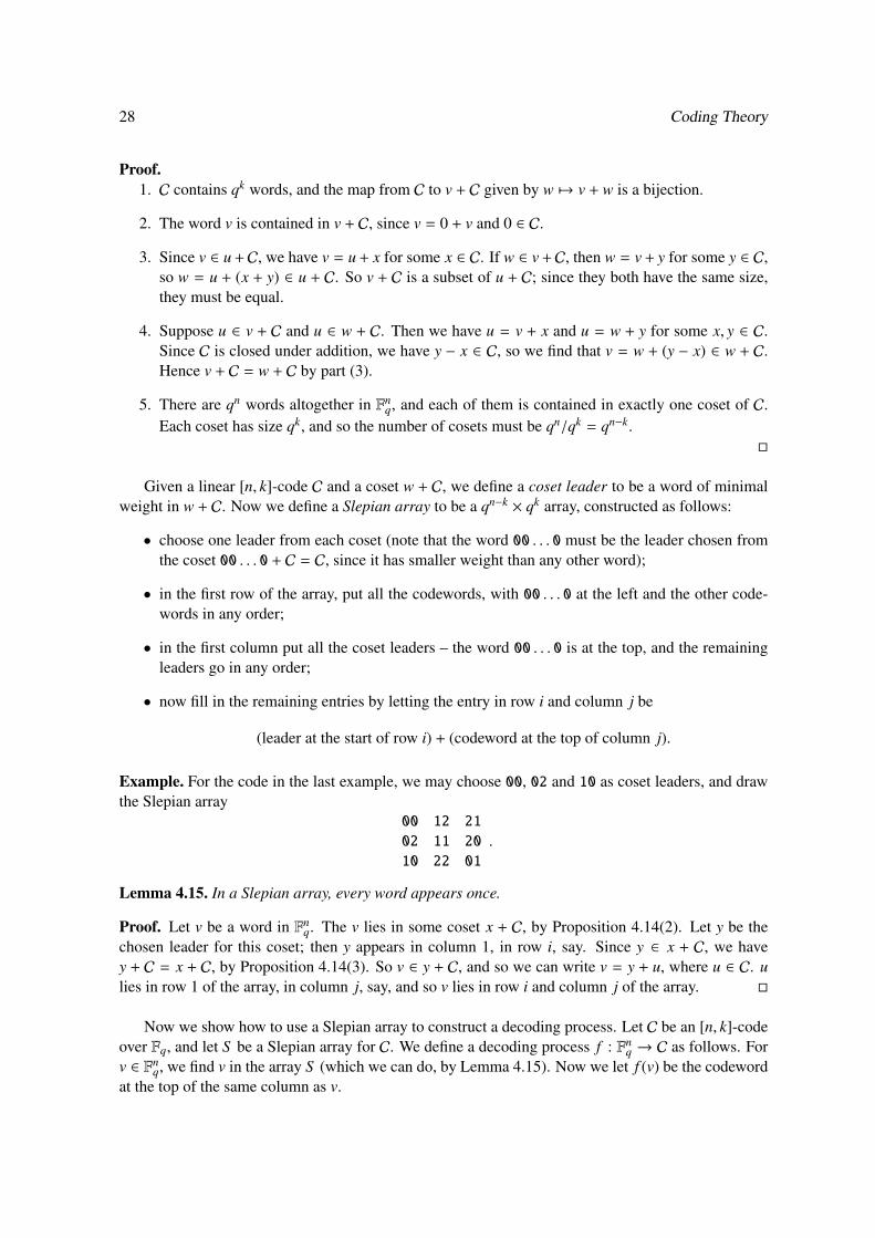
Given a linear [n, k]-code C and a coset w + C, we define a coset leader to be a word of minimalweight in w + C. Now we define a Slepian array to be a qn−k × qk array, constructed as follows:
• choose one leader from each coset (note that the word 00 . . . 0 must be the leader chosen fromthe coset 00 . . . 0 + C = C, since it has smaller weight than any other word);
• in the first row of the array, put all the codewords, with 00 . . . 0 at the left and the other code-words in any order;
• in the first column put all the coset leaders – the word 00 . . . 0 is at the top, and the remainingleaders go in any order;
• now fill in the remaining entries by letting the entry in row i and column j be
(leader at the start of row i) + (codeword at the top of column j).
Example. For the code in the last example, we may choose 00, 02 and 10 as coset leaders, and drawthe Slepian array
00 12 21
02 11 20
10 22 01
.
Lemma 4.15. In a Slepian array, every word appears once.
Proof. Let v be a word in Fnq. The v lies in some coset x + C, by Proposition 4.14(2). Let y be the
chosen leader for this coset; then y appears in column 1, in row i, say. Since y ∈ x + C, we havey + C = x + C, by Proposition 4.14(3). So v ∈ y + C, and so we can write v = y + u, where u ∈ C. ulies in row 1 of the array, in column j, say, and so v lies in row i and column j of the array. �
Now we show how to use a Slepian array to construct a decoding process. Let C be an [n, k]-codeover Fq, and let S be a Slepian array for C. We define a decoding process f : Fn
q → C as follows. Forv ∈ Fn
q, we find v in the array S (which we can do, by Lemma 4.15). Now we let f (v) be the codewordat the top of the same column as v.

Linear codes 29
Theorem 4.16. f is a nearest-neighbour decoding process.
Proof. We need to show that for any v ∈ Fnq and any w ∈ C,
d(v, f (v)) 6 d(v,w).
Find v in the Slepian array, and let u be the word at the start of the same row as v. Then, by theconstruction of the Slepian array,
v = u + f (v) ∈ u + C.
This givesv − w = u + ( f (v) − w) ∈ u + C.
Of course u ∈ u + C, and u was chosen to be a leader for this coset, which means that
weight(u) 6 weight(v − w).
So (by Lemma 4.3)d(v, f (v)) = weight(u) 6 weight(v − w) = d(v,w).
�
Example. Let q = 2, and consider the repetition code
C = {000, 111}.
A Slepian array for this is000 111
001 110
010 101
100 011
.
So if we receive the word 101, we decode it as 111, and as long as no more than one error has beenmade in transmission, this is right. Notice, in fact, that all the words in the first column are distance 1away from 000, and all the words in the second column are distance 1 away from 111.
It looks as though there’s a problem with constructing Slepian arrays, which is that we need towrite out all the cosets of C beforehand so that we can find coset leaders. In fact, we don’t.
Algorithm for constructing a Slepian array
Row 1: Write the codewords in a row, with the word 00 . . . 0 at the start, and the remaining codewordsin any order.
The other rows: For the remaining rows: if you’ve written every possible word, then stop. Other-wise, choose a word u that you haven’t written yet of minimal weight. Put u at the start of therow, and then for the rest of the row, put
u + (codeword at the top of column j)
in column j.
This is a much better way to construct Slepian arrays, since we only need to know the code, notthe cosets. However, we’ll see that we can do better than to use a Slepian array in the next section.

30 Coding Theory
5 Dual codes and parity-check matrices
5.1 The dual code
We begin by defining a scalar product on Fnq. Given words
x = (x1 . . . xn), y = (y1 . . . yn),
we definex.y = x1y1 + · · · + xnyn ∈ Fq.
You should be familiar with this from linear algebra.
Lemma 5.1. The scalar product . is symmetric and bilinear, i.e.
v.w = w.v
and(λv + µv′).w = λ(v.w) + µ(v′.w)
for all words v, v′,w and all λ, µ ∈ Fq.
Proof.
v.w =n∑
i=1
viwi
=
n∑i=1
wivi
(since multiplication in Fq is commutative)
= w.v.
Also,
(λv + µv′).w =n∑
i=1
(λv + µv′)iwi
=
n∑i=1
(λvi + µv′i)wi
= λ
n∑i=1
viwi + µ
n∑i=1
v′iwi
(since multiplication in Fq is distributive over addition)
= λ(v.w) + µ(v′.w).
�
Now, given a subspace C of Fnq, we define the dual code to be
C⊥ = {w ∈ Fnq | v.w = 0 for all v ∈ C}.
In linear algebra, we would call C⊥ the subspace orthogonal to C. We’d like a simple criterionthat tells us whether a word lies in C⊥.
Dual codes and parity-check matrices 31
Lemma 5.2. Suppose C is a linear [n, k]-code and G is a generator matrix matrix for C. Then
w ∈ C⊥ ⇔ GwT = 0.
Note that we think of the elements of Fnq as row vectors; if w is the row vector (w1 . . .wn), then wT
is the column vector w1...
wn
.G is a k × n matrix, so GwT is a column vector of length k.Proof. Suppose G has entries gi j, for 1 6 i 6 k and 1 6 j 6 n. Let gi denote the ith row of G. Theng1, . . . , gk are words which form a basis for C, and
gi = gi1 . . . gin.
Now
(GwT)i =
n∑j=1
gi jw j
= gi.w,
so GwT = 0 if and only if gi.w = 0 for all i.
(⇒) If w ∈ C⊥, then v.w = 0 for all v ∈ C. In particular, gi.w = 0 for i = 1, . . . , k. So GwT = 0.
(⇐) If GwT = 0, then gi.w = 0 for i = 1, . . . , k. Now g1, . . . , gk form a basis for C, so any v ∈ C canbe written as
v = λ1g1 + · · · + λkgk
for λ1, . . . , λk ∈ Fq. Then
v.w = (λ1g1 + · · · + λkgk).w
= λ1(g1.w) + · · · + λk(gk.w)
by Lemma 5.1
= 0 + · · · + 0.
So w ∈ C⊥.
�
This lemma gives us another way to think of C⊥ – it is the kernel of any generator matrix of C.
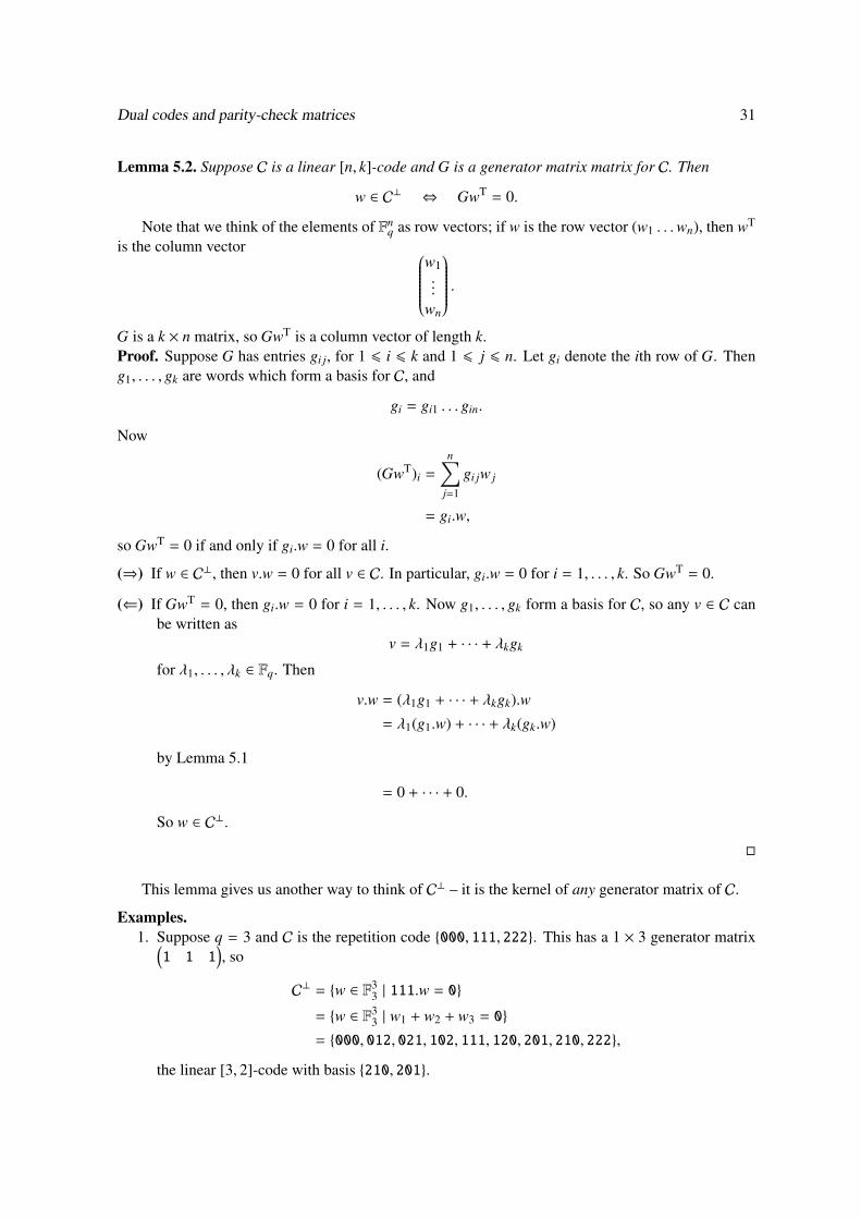
Examples.1. Suppose q = 3 and C is the repetition code {000, 111, 222}. This has a 1 × 3 generator matrix(1 1 1
), so
C⊥ = {w ∈ F33 | 111.w = 0}
= {w ∈ F33 | w1 + w2 + w3 = 0}
= {000, 012, 021, 102, 111, 120, 201, 210, 222},
the linear [3, 2]-code with basis {210, 201}.
32 Coding Theory
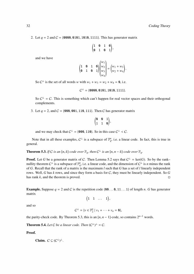
2. Let q = 2 and C = {0000, 0101, 1010, 1111}. This has generator matrix(1 0 1 0
0 1 0 1
),
and we have (1 0 1 0
0 1 0 1
) w1w2w3w4
=(w1 + w3w2 + w4
).
So C⊥ is the set of all words w with w1 + w3 = w2 + w4 = 0, i.e.
C⊥ = {0000, 0101, 1010, 1111}.
So C⊥ = C. This is something which can’t happen for real vector spaces and their orthogonalcomplements.
3. Let q = 2, and C = {000, 001, 110, 111}. Then C has generator matrix(0 0 1
1 1 0
),
and we may check that C⊥ = {000, 110}. So in this case C⊥ < C.
Note that in all these examples, C⊥ is a subspace of Fnq, i.e. a linear code. In fact, this is true in
general.
Theorem 5.3. If C is an [n, k]-code over Fq, then C⊥ is an [n, n − k]-code over Fq.
Proof. Let G be a generator matrix of C. Then Lemma 5.2 says that C⊥ = ker(G). So by the rank–nullity theorem C⊥ is a subspace of Fn
q, i.e. a linear code, and the dimension of C⊥ is n minus the rankof G. Recall that the rank of a matrix is the maximum l such that G has a set of l linearly independentrows. Well, G has k rows, and since they form a basis for C, they must be linearly independent. So Ghas rank k, and the theorem is proved. �
Example. Suppose q = 2 and C is the repetition code {00 . . . 0, 11 . . . 1} of length n. G has generatormatrix (
1 1 . . . 1),
and soC⊥ = {v ∈ Fn
2 | v1 + · · · + vn = 0},
the parity-check code. By Theorem 5.3, this is an [n, n − 1]-code, so contains 2n−1 words.
Theorem 5.4. Let C be a linear code. Then (C⊥)⊥ = C.
Proof.
Claim. C ⊆ (C⊥)⊥.

Dual codes and parity-check matrices 33
Proof. C⊥ = {w ∈ Fq | v.w = 0 for all v ∈ C}. This means that v.w = 0 for all v ∈ C andw ∈ C⊥. Another way of saying this is that if v ∈ C, then w.v = 0 for all w ∈ C⊥. So
v ∈ {x | w.x = 0 for all w ∈ C⊥} = (C⊥)⊥.
If C is an [n, k]-code, then Theorem 5.3 says that C⊥ is an [n, n − k]-code. By applying Theorem 5.3again, we find that (C⊥)⊥ is an [n, k]-code. So we have (C⊥)⊥ > C and dim(C⊥)⊥ = dimC have thesame dimension, and so (C⊥)⊥ = C. �
Now we make a very important definition.
Definition. Let C be a linear code. A parity-check matrix for C is a generator matrix for C⊥.
We will see in the rest of the course that parity-check matrices are generally more useful thangenerator matrices. Here is an instance of this.
Lemma 5.5. Let C be a code, H a parity-check matrix for C, and v a word in Fnq. Then v ∈ C if and
only if HvT = 0.
Proof. By Theorem 5.4 we have v ∈ C if and only if v ∈ (C⊥)⊥. Now H is a generator matrix for C⊥,and so by Lemma 5.2 we have w ∈ (C⊥)⊥ if and only if HwT = 0. �
But can we find a parity-check matrix? The following lemma provides a start.
Lemma 5.6. Suppose C is a linear [n, k]-code with generator matrix G, and let H be any n − k by nmatrix. Then H is a parity-check matrix for C if and only if
• the rows of H are linearly independent, and
• GHT = 0.
Proof. Let h1, . . . , hn−k be the rows of H. Then the ith column of GHT is GhTi , so GHT = 0 if and
only if GhTi = 0 for i = 1, . . . , n − k.
(⇒) If H is a parity-check matrix for C, then it is a generator matrix for C⊥, so its rows h1, . . . , hn−k
form a basis for C⊥; in particular, they are linearly independent. Also, since h1, . . . , hn−k lie inC⊥, we have GhT
i = 0 for each i by Lemma 5.2, so GHT = 0.
(⇐) Suppose that GHT = 0 and the rows of H are linearly independent. Then GhTi = 0 for each i,
and so h1, . . . , hn−k lie in C⊥ by Lemma 5.2. So the rows of H are linearly independent wordsin C⊥. But the dimension of C⊥ is n − k (the number of rows of H), so in fact these rows forma basis for C⊥, and hence H is a generator matrix for C⊥, i.e. a parity-check matrix for C.
�
This helps us to find a parity-check matrix if we already have a generator matrix. If the generatormatrix is in standard form, then a parity-check matrix is particularly easy to find.
Lemma 5.7. Suppose C is a linear code, and that
G = (Ik|A)

34 Coding Theory
is a generator matrix for C in standard form: Ik is the k by k identity matrix, and A is some k by n − kmatrix. Then the matrix
H = (−AT|In−k)
is a parity-check matrix for C.
Proof. Certainly H is an n− k by n matrix. The last n− k columns of H are the standard basis vectors,and and so are linearly independent. So H has rank at least n − k, and hence the rows of H must belinearly independent. It is a simple exercise (which you should do!) to check that GHT = 0, and wecan appeal to Lemma 5.6. �
Example.
• Recall the generator matrix (10110
01101
)for the binary (5, 4, 3)-code discussed earlier. You should check that1110010010
01001
is a parity-check matrix – remember that in F2, + and − are the same thing.
• The ternary ‘parity-check’ [3, 2]-code
{000, 012, 021, 102, 111, 120, 201, 210, 222}
has generator matrix (102
012
)and parity-check matrix
(111).
In view of Lemma 5.7, we say that a parity-check matrix is in standard form if it has the form
(B|In−k).
5.2 Syndrome decoding
Definition. Suppose C is a linear [n, k]-code over Fq, and H is a parity-check matrix for C. Then forany word w ∈ Fn
q, the syndrome of w is the vector
S (y) = yHT ∈ Fn−kq .
We saw above that w ∈ (C⊥)⊥ if and only if HwT = 0, i.e. if and only if S (y) = 0. So the syndromeof a word tells us whether it lies in our code. In fact, the syndrome tells us which coset of our codethe word lies in.

Dual codes and parity-check matrices 35
Lemma 5.8. Suppose C is a linear [n, k]-code, and v,w are words in Fnq. Then v and w lie in the same
coset of C if and only if S (v) = S (w).
Proof.
v and w lie in the same coset⇔ v ∈ w + C
⇔ v = w + x, for some x ∈ C
⇔ v − w ∈ C
⇔ H(vT − wT) = 0
⇔ HvT − HwT = 0
⇔ HvT = HwT
⇔ S (v) = S (w).
�
In view of this lemma, we can talk about the syndrome of a coset to mean the syndrome of a wordin that coset. Note that if C is an [n, k]-code, then a syndrome is a row vector of length n − k. Sothere are qn−k possible syndromes. But we saw after Proposition 4.14 that there are also qn−k differentcosets of C, so in fact each possible syndrome must appear as the syndrome of a coset.
The point of this is that we can use syndromes to decode a linear code without having to write outa Slepian array. We construct a syndrome look-up table as follows.
1. Choose a parity-check matrix H for C.
2. Choose a set of coset leaders (i.e. one leader from each coset) and write them in a list.
3. For each coset leader, calculate its syndrome and write this next to it.
Example. Let q = 3, and consider the repetition code
C{000, 111, 222}
again. This has generator matrixG = (111),
and hence parity-check matrix
H =(102
012
).
There are 9 cosets of C, and a set of coset leaders, with their syndromes, is
leader syndrome000 00
001 22
002 11
010 01
020 02
100 10
200 20
012 12
021 21
.

36 Coding Theory
Given a syndrome look-up table for a code C, we can construct a decoding process as follows.
• Given a word w ∈ Fnq, calculate the syndrome S (w) of w.
• Find this syndrome in the syndrome look-up table; let v be the coset leader with this syndrome.
• Define g(w) = w − v.
Lemma 5.9. The decoding process g that we obtain for C using a syndrome look-up table with cosetleaders l1, . . . , lr is the same as the decoding process f that we obtain using a Slepian array with cosetleaders l1, . . . , lr.
Proof. When we decode w using g, we find the coset leader with the same syndrome as w; by Lemma5.8, this means the leader in the same coset as w. So
g(w) = w − (chosen leader in the same coset as w).
When we decode using f , we set
f (w) = (codeword at the top of the same column as w).
The construction of a Slepian array means that
w = (leader at the left of the same row as w) + (codeword at the top of the same column as w),
so
f (w) = w − (leader at the left of the same row as w)
= w − (leader in the same coset as w)
(since the words in any one row of a Slepian array form a coset)
= g(w).
�
So we have seen the advantages of linear codes – although there might often be slightly largernon-linear codes with the same parameters, it requires a lot more work to describe them and to encodeand decode.
Now we’ll look at some specific examples of codes.
6 Some examples of linear codes
We’ve already seen some dull examples of codes. Here, we shall see some more interesting codeswhich are good with regard to certain bounds. The Hamming codes are perfect (i.e. give equality inthe Hamming bound); in fact, they are almost the only known perfect codes. MDS codes are codeswhich give equality in the Singleton bound. We’ll also see another bound – the Gilbert–Varshamovbound – which gives lower bounds for Aq(n, d) in certain cases.

Some examples of linear codes 37
6.1 Hamming codes
We begin with binary Hamming codes, which are slightly easier to describe.
Definition. Let r be any positive integer, and let Hr be the r by 2r − 1 matrix whose columns are allthe different non-zero vectors over F2. Define the binary Hamming code Ham(r, 2) to be the binary[2r − 1, 2r − r − 1]-code with Hr as its parity-check matrix.
Example.
• For r = 1, we haveH = (1),
so that Ham(1, 2) is the [1, 0]-code {0}.
• For r = 2, we can choose
H =(101
011
),
and Ham(2, 2) is simply the repetition code {000, 111}.
• r = 3 provides the first non-trivial example. We choose h to be in standard form:
H =
11011001011010
0111001
.Then we can write down the generator matrix
G =
1000110
0100101
0010011
0001111
.Hence
Ham(3, 2) = {0000000, 1000110, 0100101, 1100011, 0010011, 1010101, 0110110, 1110000,
0001111, 1001001, 0101010, 1101100, 0011100, 1011010, 0111001, 1111111}.
Note that the Hamming code is not uniquely defined – it depends on the order you choose for thecolumns of H. But choosing different orders still gives equivalent codes, so we talk of the Hammingcode Ham(r, 2).
Now we consider q-ary Hamming codes for an arbitrary prime power q. We impose a relation onthe non-zero vectors in Fr
q by saying that v ≡ w if and only if v = λw for some non-zero λ ∈ Fq.
Lemma 6.1. ≡ is an equivalence relation.
Proof. We need to check three things.
1. v ≡ v for all v ∈ Frq. This follows because v = 1v and 1 ∈ Fq \ {0}.
2. (v ≡ w) ⇒ (w ≡ v) for all v,w ∈ Frq. This follows because if v = λw for λ ∈ Fq \ {0}, then
w = λ−1v with λ−1 ∈ Fq \ {0}.

38 Coding Theory
3. (v ≡ w ≡ x) ⇒ (v ≡ x) for all v,w, x ∈ Frq. This follows because if v = λw and w = µx for
λ, µ ∈ Fq \ {0}, then v = (λµ)x with λµ ∈ Fq \ {0}.
�
Now we count the equivalence classes of non-zero words (the zero word lies in an equivalenceclass on its own).
Lemma 6.2. Under the equivalence relation ≡, there are exactlyqr − 1q − 1
equivalence classes of non-
zero words.
Proof. Take v ∈ Frq \ {0}. The equivalence class containing v consists of all words λv for λ ∈ Fq \ {0}.
There are q − 1 possible choices of λ, and these give distinct words: if λ , µ, then (since v , 0)(λv , µv). So there are exactly q−1 words in each equivalence class. There are qr −1 non-zero words
altogether, so the number of equivalence classes isqr − 1q − 1
. �
Now choose vectors v1, . . . , vN , where N = (qr − 1)/(q − 1), choosing exactly one from eachequivalence class. Define H to be the r by N matrix with columns v1, . . . , vN , and define the q-aryHamming code Ham(r, q) to the [N,N− r]-code over Fq with parity-check matrix H. Again, the actualcode depends on the order of v1, . . . , vN (and on the choice of v1, . . . , vN), but different choices giveequivalent codes.
Example.
• Let q = 5 and r = 2. H may be chosen to equal(111110
123401
),
so that Ham(2, 5) is the [6, 4]-code over F5 with generator matrix100044
010043
001042
000141
.• Let q = 3 and r = 3. H may be chosen to be00111111111001100111222010
1212012012001
,and Ham(3, 3) is the [13, 10]-code with generator matrix
1000000000022
0100000000021
0010000000202
0001000000201
0000100000220
0000010000222
0000001000221
0000000100210
0000000010212
0000000001211
.

Some examples of linear codes 39
It may not be obvious how to choose the vectors v1, . . . , vN , but there is a trick: choose all non-zero vectors whose first non-zero entry is a 1. You might like to prove as an exercise that this alwaysworks, but you can use this trick without justification in the exam.
Lemma 6.3. Ham(r, q) is an [N,N − r]-code over Fq, where as above N = (qr − 1)/(q − 1).
Proof. H is an r × N matrix, and so Ham(r, q)⊥ is an [N, r]-code. So Ham(r, q) is an [N,N − r]-code,by Theorem 5.3. �
Now we’ll see the key property of Hamming codes.
Theorem 6.4. Ham(r, q) has minimum distance at least 3.
Proof. Since Ham(r, q) is linear, it’s enough to show that the minimum weight of a non-zero codewordis 3, i.e. that there are no codewords of weight 1 or 2. We have a parity-check matrix H, and by Lemma5.5 a word w lies in Ham(r, q) if and only if HwT = 0. So all we need to do is show that HwT , 0whenever w is a word of weight 1 or 2.
Suppose that w has weight 1, with
wi = λ , 0,
w j = 0 for j , i.
Recall that the columns of H are v1, . . . , vN . We calculate that HwT = λvi. Now vi , 0 by construction,and λ , 0, and so HwT , 0, so w < Ham(r, q).
Next suppose w has weight 2, with
wi = λ , 0,
w j = µ , 0,
wk = 0 for k , i, j.
Then we calculate that HwT = λvi + µv j. If this equals 0, then we have
vi −µ
λv j
(since λ , 0), and this implies that vi ≡ v j (since µ , 0). But we chose v1, . . . , vN to be from differentequivalence classes; contradiction. So HwT , 0, and w < Ham(r, q). �
Theorem 6.5. Ham(r, q) is a perfect 1-error-correcting code.
Proof. Ham(r, q) is 1-error-correcting since its minimum distance is greater than 2. To show that it isperfect, we have to show that equality holds in the Hamming bound, i.e.
|Ham(r, q)| =qN(
N0
)+ (q − 1)
(N1
) ,where N =
qr − 1q − 1
.

40 Coding Theory
Since Ham(r, q) is an [N,N−r]-code, the left-hand side equals qN−r by Lemma 4.5. The right-handside equals
qN
1 + (q − 1)N=
qN
1 + (q − 1) qr−1q−1
=qN
1 + qr − 1= qN−r,
and the equation follows. �
For binary Hamming codes, there is quite a neat way to do syndrome decoding. First, we need toknow what the coset leaders look like in a Hamming code.
Lemma 6.6. Suppose C = Ham(r, q), and that D is a coset of C. Then D contains a unique word ofweight at most 1.
Proof. First we’ll show that the number of words in Frq equals the number of cosets, so that there is
one word of weight at most 1 per coset on average. Then we’ll show that any coset contains at mostone word of weight 1. This will then imply that each coset contains exactly one word of weight 1.C is an [N,N − r]-code, so there are qr cosets of C (see the discussion after Proposition 4.14).
Now we look at the number of words of weight at most 1. There is one word of weight 0. To specifya word of weight 1, we need to choose what the non-zero entry in the word will be (q − 1 choices),and where it will occur (N choices). So the number of words of weight at most 1 is
1 + (q − 1)N = 1 + (q − 1)qr − 1q − 1
= qr.
For the second part, suppose v and w are weight at most 1 lying in the same coset. Then v ∈ w+C,so v = w + x for some x ∈ C, i.e. v − w ∈ C. Now v and −w are words of weight at most 1, and sov − w has weight at most 2. But d(C) > 3, so the only word in C of weight at most 2 is the zero word.So v − w = 0, i.e. v = w, and so a coset contains at most one word of weight at most 1. �
The preceding lemma tells us that the coset leaders for a Hamming code must be precisely allthe words of weight at most 1. Now we restrict our attention to the case q = 2. Recall that thecolumns of Hr are precisely all the different non-zero column vectors over F2 – these give the binaryrepresentations of the numbers 1, 2, . . . , 2r − 1. We order the columns of Hr so that column i gives thebinary representation of the number i.
Example. Suppose r = 3. Then we choose 00011110110011
1010101
.Now suppose w ∈ FN
2 . Since Ham(r, 2) is perfect 1-error-correcting, w is either a codeword or isdistance 1 away from a unique codeword. So either w ∈ Ham(r, 2) or w − e j ∈ Ham(r, 2) for some(unique) j, where e j is the word which has a 1 in position j and 0s elsewhere.
If w < Ham(r, 2), we want to be able to work out what j is.

Some examples of linear codes 41
Lemma 6.7. Let S (w) be the syndrome of w. If w ∈ C, then S (w) = 0. Otherwise, S (w) gives thebinary representation of j.
Proof. Since w − e j lies in the code, e j must lie in the same coset as w. So e j has the same syndromeas w. But clearly the syndrome of e j is the jth row of HT, and we picked H so that the jth row of HT
is the binary representation of j. �
Example. Continuing the last example: suppose the codeword 0101010 is transmitted (exercise:check that this is a codeword, given the way we’ve chosen Hr). Suppose that the fifth digit getsdistorted to a 1, so we receive 0101110. We calculate the syndrome
0101110
001
010
011
100
101
110
111
= (101),
which is the binary representation of the number 5. So we know to change the fifth digit to recoverthe codeword.
6.2 Existence of codes and linear independence
The proof that the Hamming codes have distance 3 relied on the following fact about their parity-check matrices: if we take a set consisting of at most 2 columns of H, then this set is linearly inde-pendent. This leads to a more general theorem on the existence of linear codes.
Theorem 6.8. Suppose C is an [n, k]-code with parity-check matrix H. Then C has minimum distanceat least d if and only if any d − 1 columns of H are linearly independent.
In particular, an [n, k, d]-code exists if and only if there is a sequence of n vectors in Fn−kq such
that any d − 1 of them are linearly independent.
Proof. Let c1, . . . , cn be the columns of H, and suppose first that there are columns ci1 , . . . , cid−1 whichare linearly dependent, i.e. there are scalars λ1, . . . , λd−1 (not all zero) such that
λ1ci1 + · · · + λd−1cid−1 = 0.
Let w be the word which has λ1, . . . , λd−1 in positions i1, . . . , id−1, and 0s elsewhere. Then the aboveequation is the same as saying HwT = 0, which, since H is a parity-check matrix for C, is the same assaying w ∈ C. But then w is a non-zero word of weight at most d − 1, while C is a code of minimumdistance at least d; contradiction.
The other direction is basically the same: if C does not have minimum distance at least d, then Chas a non-zero codeword w of weight e < d, and the equation HwT = 0 provides a linear dependencebetween some e of the columns of H; if e vectors are linearly dependent, then any d − 1 vectorsincluding these e are certainly linearly dependent.
The second paragraph of the proposition is now immediate – if we have such a code, then thecolumns of a parity-check matrix are such a set of vectors, while if we have such a set of vectors, then

42 Coding Theory
the matrix with these vectors as its columns is the parity-check matrix of such a code. �
Notice that we say ‘sequence’ rather than ‘set’, since two columns of a matrix might be the same.However, if there are two equal columns, then they are linearly dependent, and so the minimumdistance of our code would be at most 2.
Theorem 6.8 tells us that one way to look for good linear codes is to try to find large sets ofvectors such that large subsets of these are linearly independent. This is often referred to as the ‘mainlinear coding theory problem’. We use this now to prove the Gilbert–Varshamov bound. The boundswe saw earlier – the Hamming, Singleton and Plotkin bounds – were all essentially of the form ‘if acode with these parameters exists, then the following inequality holds’, and and so gave upper boundson Aq(n, d). The Gilbert–Varshamov bound says ‘if this inequality holds, then a code with theseparameters exists’, and so it gives some lower bounds on Aq(n, d).
First we prove a very simple lemma.
Lemma 6.9. For any n, i > 0, (ni
)>
(n − 1
i
).
Proof. This follows from the equation (ni
)=
(n − 1
i
)+
(n − 1i − 1
).
This is proved either by writing the binomial coefficients in terms of factorials or by considering(ni
)as the number of ways of choosing a subset of size i from the set {1, . . . , n}. Each such subset eithercontains the number n or it doesn’t; if it doesn’t, then the set is actually a subset of {1, . . . , n − 1} ofsize i, which may be chosen in
(n−1
i
)ways. If it does, then the remainder of the subset is a subset of
{1, . . . , n − 1} of size i − 1, which may be chosen in(n−1i−1
)ways. �
Theorem 6.10 (Gilbert–Varshamov bound). Suppose q is a prime power, and n, r, d are positive inte-gers satisfying(
n − 10
)+ (q − 1)
(n − 1
1
)+ (q − 1)2
(n − 1
2
)+ · · · + (q − 1)d−2
(n − 1d − 2
)< qr. (∗)
Then an [n, n − r, d]-code over Fq exists.
Proof. By Theorem 6.8, all we need to do is find a sequence of n vectors in Frq such that any d − 1
of them are linearly independent. In fact, we can do this in a completely naıve way. We begin bychoosing any non-zero vector v1 ∈ F
rq. Then we choose any vector v2 such that v1 and v2 are linearly
independent. Then we choose any v3 such that any d − 1 of v1, v2, v3 are linearly independent, and soon. We need to show that this always works, i.e. at each stage you can choose an appropriate vector.Formally, this amounts to the following.
We prove the Gilbert–Varshamov bound by induction on n. For the case n = 1, we just need to beable to find a non-zero vector v1; we can do this, since r > 0.
Now suppose n > 1 and that the theorem is true with n replaced by n − 1, i.e. whenever(n − 2
0
)+ (q − 1)
(n − 2
1
)+ (q − 1)2
(n − 2
2
)+ · · · + (q − 1)d−2
(n − 2d − 2
)< qr, (†)
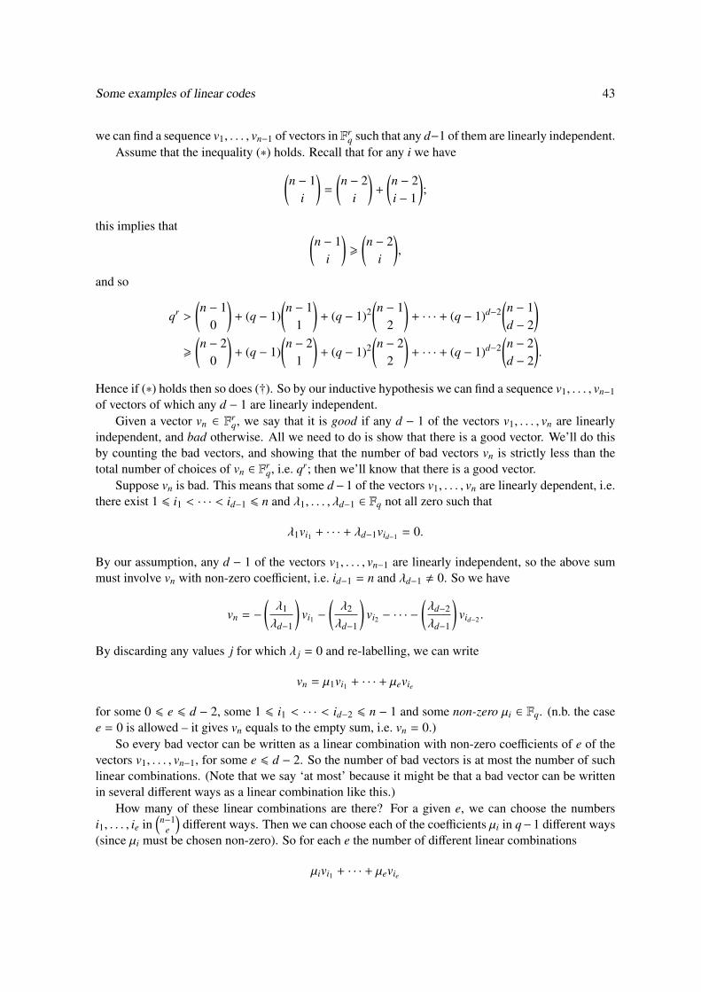
Some examples of linear codes 43
we can find a sequence v1, . . . , vn−1 of vectors in Frq such that any d−1 of them are linearly independent.
Assume that the inequality (∗) holds. Recall that for any i we have(n − 1
i
)=
(n − 2
i
)+
(n − 2i − 1
);
this implies that (n − 1
i
)>
(n − 2
i
),
and so
qr >
(n − 1
0
)+ (q − 1)
(n − 1
1
)+ (q − 1)2
(n − 1
2
)+ · · · + (q − 1)d−2
(n − 1d − 2
)>
(n − 2
0
)+ (q − 1)
(n − 2
1
)+ (q − 1)2
(n − 2
2
)+ · · · + (q − 1)d−2
(n − 2d − 2
).
Hence if (∗) holds then so does (†). So by our inductive hypothesis we can find a sequence v1, . . . , vn−1of vectors of which any d − 1 are linearly independent.
Given a vector vn ∈ Frq, we say that it is good if any d − 1 of the vectors v1, . . . , vn are linearly
independent, and bad otherwise. All we need to do is show that there is a good vector. We’ll do thisby counting the bad vectors, and showing that the number of bad vectors vn is strictly less than thetotal number of choices of vn ∈ F
rq, i.e. qr; then we’ll know that there is a good vector.
Suppose vn is bad. This means that some d− 1 of the vectors v1, . . . , vn are linearly dependent, i.e.there exist 1 6 i1 < · · · < id−1 6 n and λ1, . . . , λd−1 ∈ Fq not all zero such that
λ1vi1 + · · · + λd−1vid−1 = 0.
By our assumption, any d − 1 of the vectors v1, . . . , vn−1 are linearly independent, so the above summust involve vn with non-zero coefficient, i.e. id−1 = n and λd−1 , 0. So we have
vn = −
(λ1
λd−1
)vi1 −
(λ2
λd−1
)vi2 − · · · −
(λd−2
λd−1
)vid−2 .
By discarding any values j for which λ j = 0 and re-labelling, we can write
vn = µ1vi1 + · · · + µevie
for some 0 6 e 6 d − 2, some 1 6 i1 < · · · < id−2 6 n − 1 and some non-zero µi ∈ Fq. (n.b. the casee = 0 is allowed – it gives vn equals to the empty sum, i.e. vn = 0.)
So every bad vector can be written as a linear combination with non-zero coefficients of e of thevectors v1, . . . , vn−1, for some e 6 d − 2. So the number of bad vectors is at most the number of suchlinear combinations. (Note that we say ‘at most’ because it might be that a bad vector can be writtenin several different ways as a linear combination like this.)
How many of these linear combinations are there? For a given e, we can choose the numbersi1, . . . , ie in
(n−1
e
)different ways. Then we can choose each of the coefficients µi in q−1 different ways
(since µi must be chosen non-zero). So for each e the number of different linear combinations
µivi1 + · · · + µevie

44 Coding Theory
is (q − 1)e(n−1
e
). We sum over e to obtain
(number of bad vectors) 6(n − 1
0
)+ (q − 1)
(n − 1
1
)+ (q − 1)2
(n − 1
2
)+ · · · + (q − 1)d−2
(n − 1d − 2
)< qr
by (∗). So not every vector is bad, and so we can find a good vector. �
6.3 MDS codes
We begin by recalling the Singleton bound, and applying it to linear codes.
Theorem 6.11 (Singleton bound for linear codes). An [n, k, d]-code over Fq satisfies
d 6 n − k + 1.
Proof. If C is an [n, k, d]-code over Fq, then C is a q-ary (n,M, d)-code, where M = qk by Lemma 4.5.Hence by Theorem 2.8(2) we have
qk 6 qn+1−d,
i.e. k 6 n + 1 − d. �
The aim of this section is to look at codes which give equality in this bound. In an [n, k]-code, thenumber n − k is called the redundancy of the code – it can be thought of as the number of redundantdigits we add to our source word to make a codeword.
Definition. A maximum distance separable code (or MDS code) of length n and redundancy r is alinear [n, n − r, r + 1]-code.
Obviously, the main question concerning MDS codes is: for which n, r does an MDS code oflength n and redundancy r exist? The answer is not known in general, but we shall prove some resultsand construct some MDS codes. Theorem 6.8 says that an MDS code of length n and redundancy rexists if and only if we can find a sequence of n vectors in Fr
q of which any r are linearly independent.Clearly if we can do this for a given value of n, then we can do it for any smaller value of n, justby deleting some of the vectors. This implies that for each r (and q) there is a maximum n (possiblyinfinite) for which an MDS code of length n and redundancy r exists. Given r, q, we write max(r, q)for this maximum. The main question about MDS codes is to find the values of max(r, q).
Note that max(r, q) may be infinite, even though there are only finitely many vectors in Fnq, because
we are allowed repeats in our sequence of vectors. Note, though, that if we have a repeated vector inour sequence, then the code cannot possibly have distance more than 2. Here is our main theorem onthe values max(r, q).
Theorem 6.12.1. If r = 0 or 1, then max(r, q) = ∞.
2. If r > q, then max(r, q) = r + 1.
3. If 2 6 r 6 q, then max(r, q) > q + 1.

Some examples of linear codes 45
It is conjectured that the bounds in (3) actually give the right values of max(r, q), except in thecases where q is even and r = 3 or q− 1, in which case MDS codes of length q+ 2 can be constructed.
The three parts of Theorem 6.12 have different proofs, and the first two are quite easy.
Proof of Theorem 6.12(1). We must show that for r = 0 or 1 and for any n and q, there exists anMDS code of length n and redundancy r. For r = 0, this means we need an [n, n, 1]-code. But thewhole of Fn
q is such a code, as we saw in Theorem 2.1.For r = 1, we want to construct a sequence of n vectors in F1
q such that the set formed by any oneof them is linearly independent. We just take each of the vectors to be the vector (1). �
Proof of Theorem 6.12(2). To show that max(r, q) > r + 1, we need to show that an MDS code oflength r + 1 and redundancy r exists. But this is an [r + 1, 1, r + 1]-code, and the repetition code issuch a code.
To show that max(r, q) 6 r+1, we have to show that we can’t find an MDS code of length r+2 andredundancy r, i.e. an [r+2, 2, r+1]-code. If we can find such a code C, then any codeD equivalent toC is also an [r+2, 2, r+1]-code. So by taking a generator matrix for C and applying matrix operationsMO1–5, we may find an [r + 2, 2, r + 1]-code with a generator matrix in standard form. This has aparity-check matrix H in standard form, i.e. of the form (B|Ir), where B is some r × 2 matrix over Fq.
Let v,w be the columns of B. By Theorem 6.8 any r of the columns of H are linearly independent,i.e. any r of the vectors v,w, e1, . . . , er are linearly independent, where e1, . . . , er are the columns ofthe identity matrix, i.e. the standard basis vectors.
Suppose the entries of v are v1, . . . , vr. First we show that v1, . . . , vr are all non-zero. If not, thenv j = 0 for some j. Then we have
v =
v1v2...
v j−10
v j+1...
vr
= v1e1 + v2e2 + · · · + v j−1e j−1 + v j+1e j+1 + · · · + vrer,
and so the r vectors v, e1, . . . , e j−1, e j+1, . . . , er are linearly dependent. Contradiction. So each v j is
non-zero. Similarly we find that the entries w1, . . . ,wr of w are non-zero. This means thatv1
w1, . . . ,
vr
wrare non-zero elements of Fq. Now there are only q − 1 < r distinct non-zero elements of Fq, and so
we must havevi
wi=
v j
w jfor some i < j. We re-write this as
v j
vi−
w j
wi= 0. Now consider the vector
vvi−
wwi
. The kth component of this vector equalsvk
vi−
wk
wi, and so we have
vvi−
wwi=
r∑k=1
(vk
vi−
wk
wi
)ek.
Now for k = i and k = j we havevk
vi−
wk
wi= 0, and so we may ignore the i and j terms to get
vvi−
wwi=
i−1∑k=1
(vk
vi−
wk
wi
)ek +
j−1∑k=i+1
(vk
vi−
wk
wi
)ek +
r∑k= j+1
(vk
vi−
wk
wi
)ek.

46 Coding Theory
So the r vectors v,w, e1, . . . , ei−1, ei+1, . . . , e j−1, e j+1, . . . , er are linearly dependent; contradiction. �
For the proof of Theorem 6.12(3), we can be a bit more clever. Given a sequence of vectorsv1, . . . , vn, we have an easy way to check whether some r of them are linearly independent. Welet A be the matrix which has these vectors as its columns. Then A is a square matrix, and so has adeterminant. And the columns of A are linearly independent if and only if the determinant is non-zero.We need to look at a particular type of determinant, called a ‘Vandermonde determinant’.
Proposition 6.13. Suppose x1, . . . , xr are distinct elements of a field F. Then the determinant∣∣∣∣∣∣∣∣∣∣∣∣∣∣∣
1 1 . . . 1x1 x2 . . . xr
x21 x2
2 . . . x2r
......
...
xr−11 xr−1
2 . . . xr−1r
∣∣∣∣∣∣∣∣∣∣∣∣∣∣∣is non-zero.
Now we can construct our codes.
Proof of Theorem 6.12(3). We need to construct a [q + 1, q + 1 − r, r + 1]-code. Label the elementsof Fq as λ1, . . . , λq in some order, and let
H =
1 1 . . . 1 0λ1 λ2 . . . λq 0λ2
1 λ22 . . . λ2
q 0...
......
...
λr−21 λr−2
2 . . . λr−2q 0
λr−11 λr−1
2 . . . λr−1q 1
.
Let C be the code with H as its parity-check matrix. Then C is a [q+ 1, q+ 1− r], code, and we claimthat C has minimum distance at least r + 1. Recall from Theorem 6.8 that this happens if and only ifany r columns of H are linearly independent. H has r rows, and so any r columns together will forma square matrix, and we can check whether the columns are linearly independent by evaluating thedeterminant. So choose r columns of H, and let J be the matrix formed by them.
If the last column of H is not one of the columns chosen, then
J =
1 1 . . . 1x1 x2 . . . xr
x21 x2
2 . . . x2r
......
...
xr−11 xr−1
2 . . . xr−1r
for some distinct x1, . . . , xr, and so det(J) , 0 by Proposition 6.13. If the last column of H is one ofthe columns chosen, then we have
J =
1 1 . . . 1 0x1 x2 . . . xr−1 0x2
1 x22 . . . x2
r−1 0...
......
...
xr−21 xr−2
2 . . . xr−2r−1 0
xr−11 xr−1
2 . . . xr−1r−1 1

Some examples of linear codes 47
for some distinct x1, . . . , xr−1. Let J′ be the matrix formed by the first r − 1 rows and the first r − 1columns. Then det(J′) , 0 by Proposition 6.13, and so the first r−1 rows of J are linearly independent.Now consider the rows of J; suppose that
µ1.(row 1) + · · · + µr−1.(row r − 1) + µr.(row r) = 0.
Looking at the last entry of each row, we see that
0 + · · · + 0 + µr = 0.
Henceµ1.(row 1) + · · · + µr−1.(row r − 1) = 0,
but this implies µ1 = · · · = µr−1 = 0, since the first r − 1 rows of J are linearly independent. And soall the rows of J are linearly independent, so det J , 0, as required. �
6.4 Reed–Muller codes
The Reed–Muller codes are binary codes, and we need to define a new operation on binary words.If v = v1 . . . vn and w = w1 . . .wn are words in Fn
2, then we define the product v ∗ w to be the word(v1w1) . . . (vnwn). Note that v.w is the weight of v ∗ w modulo 2.
Now suppose n is a positive integer and 0 6 i < n. Let xi(n) be the word of length 2n whichconsists of chunks of 0s and 1s alternately, the chunks being of length 2i.
Example. We have
x0(2) = 0101,
x1(2) = 0011,
x0(3) = 01010101,
x1(3) = 00110011,
x2(3) = 00001111.
We will write xi(n) as xi when it is clear what the value of n is. We consider products of the wordsxi(n). For example,
x0(2)x1(2) = 0001,
x0(3)x2(3) = 00000101.
We include the word 11 . . . 1, which we regard as the ‘empty product’, and write as 1(n). Notethat we only bother with products of distinct xi(n)s, since xi(n)xi(n) = xi(n).
Definition. The rth-order Reed–Muller code R(r, n) is the binary linear code of length 2n spanned byall products of at most r of the words x0(n), . . . , xn−1(n).
Note that in ‘at most r’ we include 0, so we include the product of none of the words x0(n), . . . , xn−1(n),i.e. the word 1(n).
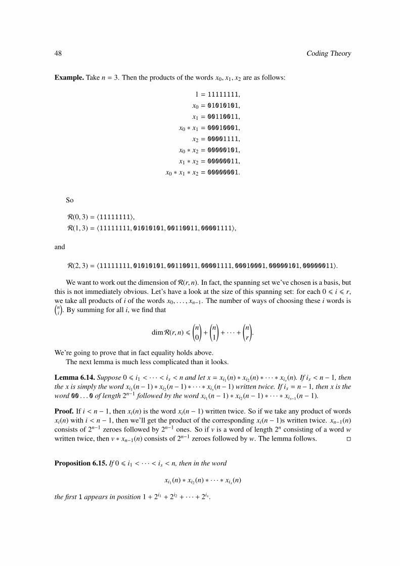
48 Coding Theory
Example. Take n = 3. Then the products of the words x0, x1, x2 are as follows:
1 = 11111111,
x0 = 01010101,
x1 = 00110011,
x0 ∗ x1 = 00010001,
x2 = 00001111,
x0 ∗ x2 = 00000101,
x1 ∗ x2 = 00000011,
x0 ∗ x1 ∗ x2 = 00000001.
So
R(0, 3) = 〈11111111〉,
R(1, 3) = 〈11111111, 01010101, 00110011, 00001111〉,
and
R(2, 3) = 〈11111111, 01010101, 00110011, 00001111, 00010001, 00000101, 00000011〉.
We want to work out the dimension of R(r, n). In fact, the spanning set we’ve chosen is a basis, butthis is not immediately obvious. Let’s have a look at the size of this spanning set: for each 0 6 i 6 r,we take all products of i of the words x0, . . . , xn−1. The number of ways of choosing these i words is(ni
). By summing for all i, we find that
dimR(r, n) 6(n0
)+
(n1
)+ · · · +
(nr
).
We’re going to prove that in fact equality holds above.The next lemma is much less complicated than it looks.
Lemma 6.14. Suppose 0 6 i1 < · · · < is < n and let x = xi1(n) ∗ xi2(n) ∗ · · · ∗ xis(n). If is < n − 1, thenthe x is simply the word xi1(n− 1) ∗ xi2(n− 1) ∗ · · · ∗ xis(n− 1) written twice. If is = n− 1, then x is theword 00 . . . 0 of length 2n−1 followed by the word xi1(n − 1) ∗ xi2(n − 1) ∗ · · · ∗ xis−1(n − 1).
Proof. If i < n − 1, then xi(n) is the word xi(n − 1) written twice. So if we take any product of wordsxi(n) with i < n − 1, then we’ll get the product of the corresponding xi(n − 1)s written twice. xn−1(n)consists of 2n−1 zeroes followed by 2n−1 ones. So if v is a word of length 2n consisting of a word wwritten twice, then v ∗ xn−1(n) consists of 2n−1 zeroes followed by w. The lemma follows. �
Proposition 6.15. If 0 6 i1 < · · · < is < n, then in the word
xi1(n) ∗ xi2(n) ∗ · · · ∗ xis(n)
the first 1 appears in position 1 + 2i1 + 2i2 + · · · + 2is .

Some examples of linear codes 49
Proof. We prove this by induction on n, with the case n = 1 being easy to check. So we suppose thatn > 1 and the result holds with n replaced by n − 1. Let x = xi1(n) ∗ xi2(n) ∗ · · · ∗ xis(n). There are twocases to consider, according to whether is = n− 1 or not. If is < n− 1, then by Lemma 6.14 x consistsof the word xi1(n−1)∗· · ·∗ xis(n−1) written twice, so the first 1 appears in position 1+2i1+ · · ·+2is , byinduction. If is = n−1, then by Lemma 6.14 x consists of the word consisting of 2n−1 zeroes followedby the word xi1(n−1) ∗ · · · ∗ xis−1(n−1). So by induction the first 1 appears in position 2n−1+ p, wherep is the position of the first 1 in xi1(n− 1) ∗ · · · ∗ xis−1(n− 1). By induction p = 1+ 2i1 + · · ·+ 2is−1 , andthe result follows. �
There are 2n different products of the words x0(n), . . . , xn−1(n) (since each xi(n) is either involvedin the product or not involved in it). Recall that for a positive integer p there is a unique way to writep − 1 as a sum of distinct powers of 2, i.e. there are unique integers i1 < i2 < · · · < is such that
p − 1 = 2i1 + · · · + 2is .
Hence there is a unique way to write
p = 1 + 2i1 + · · · + 2is .
Combined with Proposition 6.15, this means that for each p there is exactly one word which is aproduct of words xi(n) and which has its first 1 in position p. We label the products of the wordsx0(n), . . . , xn−1(n) as y1, . . . , y2n so that for each yp has its first 1 in position p, for each p.
Corollary 6.16. The words y1, . . . , y2n are linearly independent, and
dimR(r, n) =(n0
)+
(n1
)+ · · · +
(nr
).
Proof. Supposeλ1y1 + · · · + λ2ny2n = 0,
with each λi equal to 0 or 1 and not all the λi being 0. Let p be minimal such that λi = 1. The wordyp has a 1 in position p, while the words yp+1, . . . , y2n each have a 0 in position p. Hence the word
λ1w1 + · · · + λ2nw2n
has a 1 in position p; contradiction.Now for the second part. As we have seen, there are(
n0
)+
(n1
)+ · · · +
(nr
)words which are products of at most r of the words x0(n), . . . , xn−1(n). These span R(r, n) by defini-tion, and by Proposition 6.15 they are linearly independent, and so they form a basis for R(r, n). �
Now we want to find the minimum distance of R(r, n).
Theorem 6.17. R(r, n) has minimum distance 2n−r.

50 Coding Theory
Proof. (Non-examinable) We use the fact that the minimum distance of a linear code equals theminimum weight of a non-zero codeword. First we want to show that there is a codeword of weight2n−r. We claim that the word
xn−r(n) ∗ xn−r+1(n) ∗ · · · ∗ xn−1(n)
consists of 2n − 2n−r zeroes followed by 2n−r ones. We prove this by induction on n, with the casen = 1 easy to check. Suppose n > 1. By Lemma 6.14 the word xn−r(n)∗ xn−r+1(n)∗ · · · ∗ xn−1(n) equalsthe word 00 . . . 0 of length 2n−1 followed by the word
xn−r(n − 1) ∗ xn−r+1(n − 1) ∗ · · · ∗ xn−2(n − 1).
By induction this word consists of 2n−1 − 2n−r zeroes followed by 2n−r ones, and the claim is proved.Hence R(r, n) contains a word of weight 2n−r, so d(R(r, n)) 6 2n−r.
Now we show that every non-zero word has weight at least 2n−r. Again, we proceed by inductionon n, with the case n = 1 being easy to check. So we suppose that n > 1 and that the theorem is truefor n − 1. Suppose w is a non-zero word in R(r, n); then we can write
w = y1 + · · · + ys,
where each yi is a product of at most r of the words x0(n), . . . , xn−1(n). We let u be the sum of all theterms which do not include xn−1(n), and we let v be the sum of all the terms which do include xn−1(n).Then w = u + v, and by Lemma 6.14 we see that
• u consists of a word u′ ∈ R(r, n − 1) written twice, and
• v consists of 2n−1 zeroes followed by a word v′ ∈ R(r − 1, n − 1).
Now we can prove that the weight of w is at least 2n−r, by considering several cases.
• Suppose v′ = 0. Then u′ , 0, and w consists of u written twice, so weight(w) = 2 weight(u′). Byinduction, the weight of u′ is at least 2(n−1)−r, and so the weight of w is at least 2.2n−1−r = 2n−r.
• Now suppose u′ = v′. Then u′ , 0, and w consists of the word u′ followed by 2n−1 zeroes. Soweight(w) = weight(u′). Now u′ = v′ ∈ R(r − 1, n − 1), and so by induction the weight of u′ isat least 2(n−1)−(r−1) = 2n−r.
• Finally suppose u′ , v′ , 0. Then w consists of the word u′ followed by the word u′ + v′, soweight(w) = weight(u′) +weight(u′ + v′). u′ and u′ + v′ are both non-zero words in R(r, n − 1),and so by induction weight(u′) and weight(u′ + v′) are both at least 2n−1−r. Hence weight(w) >2n−1−r + 2n−1−r = 2n−r.
�