
Martin Mozinaˇ - SLAISslais.ijs.si/theses/2009-12-11-Mozina.pdf · ASPIC and X-Media. I thank John...
211
Univerza v Ljubljani Fakulteta za raˇ cunalniˇ stvo in informatiko Martin Moˇ zina Argumentirano strojno uˇ cenje DOKTORSKA DISERTACIJA Ljubljana, 2009
Transcript of Martin Mozinaˇ - SLAISslais.ijs.si/theses/2009-12-11-Mozina.pdf · ASPIC and X-Media. I thank John...

Univerza v Ljubljani
Fakulteta za racunalnistvo in informatiko
Martin Mozina
Argumentirano strojno ucenje
DOKTORSKA DISERTACIJA
Ljubljana, 2009


Univerza v Ljubljani
Fakulteta za racunalnistvo in informatiko
Martin Mozina
Argumentirano strojno ucenje
DOKTORSKA DISERTACIJA
Mentor: akad. prof. dr. Ivan Bratko
Ljubljana, 2009

University of Ljubljana
Faculty of Computer and Information Science
Martin Mozina
Argument Based Machine Learning
DOCTORAL DISSERTATION
Supervisor: Acad. Prof. Dr. Ivan Bratko
Ljubljana, 2009


Povzetek
V pricujocem delu opisemo argumentirano strojno ucenje (angl. Argument-BasedMachine Learning, s kratico ABML), ki zdruzuje strojno ucenje s tehnikami argu-mentacije. Argumenti so orodje, s katerim domenski strokovnjaki razlagajo relacijemed atributi in razredom za posamezne ucne primere. Primeri razlozeni z argu-menti se imenujejo argumentirani ucni primeri. Cilj ucenja v ABML je poiskatitako hipotezo v prostoru vseh moznih hipotez, ki uporabi dane argumente za razlagorazreda argumentiranih ucnih primerov. S tem argumenti omejujejo prostor spre-jemljivih hipotez, kar zmanjsa moznost prevelikega prilagajanja podatkom in hkrativodijo ucni algoritem k hipotezam, ki so razumljivejse.
Ena glavnih razlik med ABML in ostalimi metodami, ki omogocajo uporabopredznanja, je v nacinu izvabljanja znanja s strani domenskih strokovnjakov. Prob-lem vecine obstojecih metod za strojno ucenje je, da zahtevajo splosno domenskoznanje. Pridobivanje takega predznanja predstavlja problem, imenovan Feigenbau-movo ozko grlo, saj domenski strokovnjaki pogosto niso sposobni dobro izraziti nji-hovega splosnega znanja. Izkaze se, da jim je veliko lazje razlagati znanje s pomocjoargumentov na konkretnih primerih. V okviru tega smo razvili algoritem za odkri-vanje kriticnih primerov; to so primeri, ki jih trenutno naucena hipoteza ne zna dobronapovedovati. V procesu ucenja se tako strokovnjakom pokazejo samo ti primeri,saj bi bilo nemogoce pricakovati, da nam bodo razlozili prav vse ucne primere. Stem se vedno dobimo vse relevatno znanje, ostalo znanje pa metoda odkrije iz ucnihpodatkov.
Na podlagi osnovih principov argumentiranega ucenja smo razvili metodo ABCN2,razsirjeno razlicico znanega algoritma za ucenje pravil CN2. ABCN2 se nauci karse da tocne mnozice pravil in pri tem zagotavlja, da bo med pravili, ki pokrijejo ar-gumentirane ucne primere, vsaj eno tako, ki vsebuje med svojimi pogoji razloge izargumenta. ABCN2 smo se dodatno razsirili z novo metodo EVC (angl. extremevalue correction) za korigiranje ocenjene tocnosti pravil glede na stevilo pregledanihpravil v postopku ucenja. Ta popravek se izkaze za pomembnega v argumentiranemucenju, saj se prostor preiskovanja razlikuje od pravila do pravila glede na dolzinoustreznih argumentov. Poleg tega se EVC izkaze za koristno orodje tudi pri ucenjunavadnih pravil (brez argumentov), saj so napovedne tocnosti pravil z uporabo EVCstatisticno boljse od pravil brez te korekcije.
Delo zakljucimo z eksperimentalno primerjavo ABCN2 in CN2 ter nekaterimiostalimi metodami strojnega ucenja. ABCN2 se je izkazala za boljso metodo od
i
CN2 glede na tocnost in razumljivost pravil v prav vseh izvedenih poskusih, vendarzaradi razmeroma majhnega stevila poskusov tega nismo mogli statisticno dokazati.Ker je izvajanje primerjave na dovolj velikem vzorcu domen prakticno neizvedljivo,saj pri ABCN2 vedno potrebujemo sodelovanje z domenskim strokovnjakom, karje casovno potratno, smo se odlocili za analizo vpliva nakljucnih argumentov nauspesnost ucenja z ABCN2. Izkaze se, da nakljucni atributi ne poslabsajo tocnostinaucenih modelov in iz tega sklepamo, da argumenti ne morejo poslabsati tocnostimodela, ce so le boljsi od nakljucnih.
Kljucne besede
• umetna inteligenca, strojno ucenje, argumentacija
• ucenje pravil, ucenje s predznanjem, domensko znanje
• argumentirano strojno ucenje, ABML, CN2, ABCN2, korekcija ekstremnihvrednosti
ii

Abstract
The Thesis presents a novel approach to machine learning, called ABML (argumentbased machine learning). This approach combines machine learning from exampleswith some concepts from the field of defeasible argumentation, where arguments areused together with learning examples by learning methods in the induction of a hy-pothesis. An argument represents a relation between the class value of a particularlearning example and its attributes and can be regarded as a partial explanation ofthis example. We require that the theory induced from the examples explains theexamples in terms of the given arguments. Thus arguments constrain the combinato-rial search among possible hypotheses, and also direct the search towards hypothesesthat are more comprehensible in the light of expert’s background knowledge. Argu-ments are usually provided by domain experts. One of the main differences betweenABML and other knowledge-intensive learning methods is in the way the knowledgeis elicited from these experts. Other methods require general domain knowledge, thatis knowledge valid for the entire domain. The problem with this is the difficulty thatexperts face when they try to articulate their global domain knowledge. On the otherhand, as arguments contain knowledge specific only to certain situations, they needto provide only local knowledge for the specific examples. Experiments with ABMLand other empirical observations show that experts have significantly less problemswhile expressing such local knowledge. Furthermore, we define the ABML loopthat iteratively selects critical learning examples, namely examples that could not beexplained by the current hypothesis, which are then shown to domain experts. Us-ing this loop, the burden that lies on experts is further reduced (only some examplesneed to be explained) and only relevant knowledge is obtained (difficult examples).We implemented the ABCN2 algorithm, an argument-based extension of the rulelearning algorithm CN2. The basic version of ABCN2 ensures that rules classify-ing argumented examples will contain the reasons of the given arguments in theircondition part. We furthermore improved the basic algorithm with a new method forevaluation of rules, called extreme value correction (EVC), that reduces the optimismof evaluation measures due to the large number of rules tested and evaluated duringthe learning process (known as the multiple comparison procedures problem). Thisfeature is critical for ABCN2, since arguments given to different examples have dif-ferent number of reasons and therefore differently constrain the space for differentrules. Moreover, as shown in the dissertation, using this method in CN2 (withoutarguments) results in significantly more accurate models as compared to the original
iii
CN2. We conclude this work with a set of practical evaluations and comparisonsof ABCN2 to other machine learning algorithms on several data sets. The resultsfavour ABCN2 in all experiments, however, as each experiment requires a certainamount of time due to involvement of domain experts, the number of experiments isnot large enough to allow a valid statistical test. Therefore, we explored the capa-bility of ABCN2 to deal with erroneous arguments, and showed in the dissertationthat using false arguments will not decrease the quality of the induced model. Hence,ABCN2 can not perform worse than CN2, but it can perform better given the qualityof arguments is high enough.
Keywords
• artificial intelligence, machine learning, argumentation
• rule induction, knowledge-intensive learning, background knowledge, domainknowledge
• argument based machine learning, ABML, CN2, ABCN2, extreme value cor-rection
iv

IZJAVA O AVTORSTVUdoktorske disertacije
Spodaj podpisani Martin Mozina,z vpisno stevilko 63970103,
sem avtor doktorske disertacije z naslovom
Argumentirano strojno ucenje(angl. Argument Based Machine Learning)
S svojim podpisom zagotavljam, da:
• sem doktorsko disertacijo izdelal samostojno pod vodstvom mentorja akad.prof. dr. Ivana Bratka
• so elektronska oblika doktorske disertacije, naslov (slov., angl.), povzetek (slov.,angl.) ter kljucne besede (slov., angl.) identicni s tiskano obliko doktorske dis-ertacije
• in soglasam z javno objavo elektronske oblike doktorske disertacije v zbirki“Dela FRI”.
V Ljubljani, dne 30. novembra 2009 Podpis avtorja:
v

Acknowledgements
First and foremost, my gratitude goes to Ivan Bratko, my supervisor, who gave me theopportunity to work in a relaxing, yet very productive environment. He showed mehow to carry out my research at high standards and how to successfully publish mywork. I was often amazed at his ability to see the big picture, even when I could not,and at his power to generate new ideas, when I had already hit the wall. I appreciatethe time and effort offered by the members of my reading committee: Blaz Zupan,Saso Dzeroski, and Floriana Esposito.
I would like to thank to all members of the Artificial Intelligence Laboratoryfor providing a great working environment. I particularly appreciate help from JureZabkar, who helped a lot during the development of the ABCN2 algorithm and healso introduced me to Jerneja Videcnik, who kindly provided data and her expertisefor the infections-in-the-elderly-population domain, one of the earliest experimentswith ABCN2 . I sincerely thank the co-authors Janez Demsar and Blaz Zupan forhelping me to get my first paper published at the ECML’04 conference, which was avery nice experience for me at that time. I also thank them for their work on Orange, alibrary of machine learning methods that tremendously simplified prototyping of newalgorithms. Furthermore, I must thank Sasa Sadikov, Matej Guid, and Jana Krivec, allexperts in chess, who are developing the chess tutoring application where many ma-chine learning problems were identified and best solved by argument-based machinelearning. Following are the rest of the lab members who were always ready to listenand provide their comments (if they could only understand me): Tadej Janez, AljazKosmerlj, Damjan Kuznar, Blaz Strle, Tomaz Curk, Gregor Leban, Minca Mramor,Lan Umek, Marko Toplak, Miha Stajdohar, Lan Zagar and Jure Zbontar, and somepast members: Peter Juvan, Daniel Vladusic, Dorian Suc and Aleks Jakulin.
My research work in the past years was supported by two European projects,ASPIC and X-Media. I thank John Fox for coordinating ASPIC, the project thatinspired most of the work in this Thesis. Trevor Bench-Capon provided the data forWelfare Benefit Approval, which was the first successful experiment with ABML. Ialso sincerely thank Henry Prakken, Martin Caminada, Sanjay Modgil, Matt South,and Pancho Tolchinsky for answering so many questions I had about argumentation.After ASPIC, I joined the X-Media project, lead by Fabio Ciravegna, which wasconceptually a very different project. However, with Claudio Giuliano we were ableto identify a way to combine learning from text with learning from data through theuse of ABML. Some principles of ABML were also used in the Fiat application for
vii

noise reduction in cars. This problem was defined by Marina Giordanino and the Fiataerodynamics department.
I should not forget to thank the ladies from the Dean’s office and the Studentoffice who helped me a lot with all sorts of administrative issues: Dragica Furlan,Milica Vidic, Maja Kerkez, Mira Skrlj, Lucija Zavrsnik and Jasna Bevk.
This dissertation is dedicated to my parents Janez and Alenka, my brother Miha,my wife Janja and my two beautiful daughters Tjasa and Katja.
Martin Mozina
viii

Contents
1 Introduction 11.1 Overview of the dissertation . . . . . . . . . . . . . . . . . . . . . 41.2 Contributions of the dissertation . . . . . . . . . . . . . . . . . . . 5
I Fundamental Principles andRelated Work 7
2 Expert Knowledge inMachine Learning 92.1 Machine learning . . . . . . . . . . . . . . . . . . . . . . . . . . . 92.2 Why use domain knowledge? . . . . . . . . . . . . . . . . . . . . . 112.3 An overview of using knowledge in learning . . . . . . . . . . . . . 142.4 Formal definition of learning with prior knowledge . . . . . . . . . 17
3 Introduction to Argumentation 193.1 An argument . . . . . . . . . . . . . . . . . . . . . . . . . . . . . . 213.2 Reasoning with arguments . . . . . . . . . . . . . . . . . . . . . . 223.3 Argumentation and machine learning . . . . . . . . . . . . . . . . . 24
II Argument Based Machine Learning and the ABCN2 Algo-rithm 25
4 Argument Based Machine Learning 274.1 An illustrating example . . . . . . . . . . . . . . . . . . . . . . . . 284.2 Motivation . . . . . . . . . . . . . . . . . . . . . . . . . . . . . . . 294.3 Formal definition of argument based machine learning . . . . . . . . 304.4 Comparison of classical and argument-based prior knowledge . . . . 35
ix

4.5 Guidelines for building argument based machine learning methods . 364.5.1 Argument based inductive logic programming . . . . . . . . 384.5.2 Argument based logistic regression . . . . . . . . . . . . . . 39
5 Argument Based Rule Learning (ABCN2) 415.1 Argumented examples . . . . . . . . . . . . . . . . . . . . . . . . . 425.2 Argument based CN2 algorithm . . . . . . . . . . . . . . . . . . . 45
5.2.1 ABCN2: covering algorithm . . . . . . . . . . . . . . . . . 455.2.2 ABCN2: search procedure. . . . . . . . . . . . . . . . . . . 475.2.3 Time complexity and optimisation . . . . . . . . . . . . . . 495.2.4 Implementation . . . . . . . . . . . . . . . . . . . . . . . . 51
6 Extensions of ABCN2 536.1 Extreme value correction . . . . . . . . . . . . . . . . . . . . . . . 53
6.1.1 Related work . . . . . . . . . . . . . . . . . . . . . . . . . 566.1.2 The general principle of extreme value correction . . . . . . 57
6.2 Extreme value correction in rule learning . . . . . . . . . . . . . . . 646.2.1 EVC algorithm for relative frequencies. . . . . . . . . . . . 666.2.2 Extreme value corrected relative frequency in PN space . . . 696.2.3 Experiments . . . . . . . . . . . . . . . . . . . . . . . . . . 716.2.4 Extreme value correction in argument based rule learning . . 736.2.5 When extreme value correction should be used? . . . . . . . 73
6.3 Probabilistic covering . . . . . . . . . . . . . . . . . . . . . . . . . 756.4 Computing parameters of extreme-value distribution . . . . . . . . . 77
7 Classification from Rules and Combining ABCN2 with Other Methods 797.1 Related work . . . . . . . . . . . . . . . . . . . . . . . . . . . . . 807.2 The PILAR algorithm . . . . . . . . . . . . . . . . . . . . . . . . . 80
7.2.1 Log-linear sum of unordered rules . . . . . . . . . . . . . . 817.2.2 Rules as constraints . . . . . . . . . . . . . . . . . . . . . . 82
7.3 Evaluation . . . . . . . . . . . . . . . . . . . . . . . . . . . . . . . 857.3.1 Linear models vs. non-linear models . . . . . . . . . . . . . 857.3.2 PILAR vs other linear models . . . . . . . . . . . . . . . . 887.3.3 Improving machine learning methods: logistic regression . . 907.3.4 Visualisation of PILAR model with a nomogram . . . . . . 90
7.4 PILAR + any method = any ABML method . . . . . . . . . . . . . 93
x
7.5 Discussion . . . . . . . . . . . . . . . . . . . . . . . . . . . . . . . 93
8 ABML Refinement Loop: Selection of Critical Examples 958.1 Identifying critical examples . . . . . . . . . . . . . . . . . . . . . 96
8.2 Are expert’s arguments good or should they be improved? . . . . . . 97
8.3 Similarity and differences with active learning . . . . . . . . . . . . 98
III Experiments and Evaluation 101
9 Introductory experiments 1039.1 Animal classification . . . . . . . . . . . . . . . . . . . . . . . . . 104
9.2 Welfare benefit approval . . . . . . . . . . . . . . . . . . . . . . . 106
9.2.1 The data set . . . . . . . . . . . . . . . . . . . . . . . . . . 107
9.2.2 Experiment with ABCN2 . . . . . . . . . . . . . . . . . . . 109
9.2.3 Discussion . . . . . . . . . . . . . . . . . . . . . . . . . . . 114
9.3 Infections in elderly population . . . . . . . . . . . . . . . . . . . . 115
9.3.1 Data . . . . . . . . . . . . . . . . . . . . . . . . . . . . . . 115
9.3.2 Arguments . . . . . . . . . . . . . . . . . . . . . . . . . . 116
9.3.3 Experiments . . . . . . . . . . . . . . . . . . . . . . . . . . 117
9.3.4 Discussion . . . . . . . . . . . . . . . . . . . . . . . . . . . 118
9.4 South Africa heart-disease domain . . . . . . . . . . . . . . . . . . 119
10 Arguments Implying New Attributes 12310.1 Japanese credit screening database . . . . . . . . . . . . . . . . . . 123
10.2 ZEUS credit assignment problem . . . . . . . . . . . . . . . . . . . 125
10.3 Construction of sophisticated chess concepts . . . . . . . . . . . . . 127
10.3.1 Experiment . . . . . . . . . . . . . . . . . . . . . . . . . . 128
10.3.2 Discussion . . . . . . . . . . . . . . . . . . . . . . . . . . . 133
11 Automatically Extracted Arguments from Text 13511.1 Extracting arguments from text . . . . . . . . . . . . . . . . . . . . 135
11.2 Case study: animal classification . . . . . . . . . . . . . . . . . . . 137
12 Can Imperfect Arguments be Damaging? 143
xi

13 Concluding Remarks and Further Work 149
A Razsirjeni povzetek v slovenskem jeziku (Extended Abstract in SloveneLanguage) 153A.1 Uvod . . . . . . . . . . . . . . . . . . . . . . . . . . . . . . . . . . 155
A.1.1 Prispevki znanosti . . . . . . . . . . . . . . . . . . . . . . . 158A.2 Argumentirano strojno ucenje . . . . . . . . . . . . . . . . . . . . . 160A.3 Argumentirano ucenje pravil . . . . . . . . . . . . . . . . . . . . . 162
A.3.1 Argumentirani ucni primeri . . . . . . . . . . . . . . . . . . 162A.3.2 ABCN2 algoritem . . . . . . . . . . . . . . . . . . . . . . . 163A.3.3 Ocenjevanje kvalitete pravila v ABCN2 . . . . . . . . . . . 164A.3.4 Algoritem PILAR: klasifikacija s pravili in popravljanje poljubne
metode strojnega ucenja . . . . . . . . . . . . . . . . . . . 167A.4 ABML ucni cikel . . . . . . . . . . . . . . . . . . . . . . . . . . . 167A.5 Eksperimenti in aplikacije . . . . . . . . . . . . . . . . . . . . . . . 168
A.5.1 Klasifikacija zivali . . . . . . . . . . . . . . . . . . . . . . 169A.5.2 Odobritev socialne pomoci . . . . . . . . . . . . . . . . . . 170A.5.3 Prognostika infekcije med starejsimi obcani . . . . . . . . . 171A.5.4 Prognostika bolezni srca . . . . . . . . . . . . . . . . . . . 172A.5.5 Odobravanje kredita (Japanese Credit Screening Database) . 172A.5.6 Konstrukcija kompleksnih sahovskih konceptov . . . . . . . 173A.5.7 Avtomatska konstrukcija argumentov iz teksta . . . . . . . . 174A.5.8 Vpliv napacnih argumentov na tocnost hipoteze . . . . . . . 175
A.6 Zakljucek . . . . . . . . . . . . . . . . . . . . . . . . . . . . . . . 175
Bibliography 181
xii

Chapter 1
Introduction
Machine learning is concerned with the development of algorithms that enable com-puter programs to learn and improve from experience [Mit97]. The most commontype of machine learning (ML) is learning from labeled examples, called also super-vised inductive learning. Each example is described by a set of descriptive attributes(inputs), and a class variable (output). The task is therefore to formulate a hypothesisin some formal language that can predict outputs of examples given inputs. This newhypothesis can be used to predict the outcome of new cases, where the true valuesare unknown. Some learning problems tackled with inductive learning are:
• Given examples of weather situations, learn to forecast weather in the future;
• Given examples of past patients, learn to diagnose new patients;
• Given examples of chess positions, determine the relative quality of particularpieces (e.g. the goodness of a bishop from strategical point of view).
Learning examples represent the past experience; cases where the outcome is al-ready known. The attributes describing them are usually some natural properties,which we hope will suffice to make good predictions. For example, a weather situa-tion can be described by wind direction, temperature, and humidity, where the classcould be the weather situation on the following day. We hope that running a learn-ing algorithm on such data will provide a hypothesis giving good prediction for newcases. However, it may also happen that the learning mechanism will fail to find ahypothesis that would predict well. This can happen either because (1) the set of
1

1. INTRODUCTION
attributes is not comprehensive, (2) the relation between classes and attributes is acomplex function and therefore hard to learn, (3) the language representing the hy-potheses is inappropriate for the learning problem, (4) or the method overfits on thegiven training data.
Whenever learning fails to produce acceptable results, the burden of improvinglies on the domain experts. If the descriptions of examples are not sufficient to explainthe outputs, they need to expand the descriptions by adding additional attributes. Ifthe language expressivity is insufficient, an alternative formal language needs to beused. When the target hypothesis is very complex and hard to find, the machinelearning algorithm needs guidance to be able to find this hypothesis. Domain expertscan provide their prior knowledge about the target hypothesis (e.g. parts of the correcthypothesis) and this knowledge can then be used to guide the learning mechanismtowards those hypotheses that seem more promising to a domain expert. The problemwith this approach is the difficulty that experts face when they try to articulate theirglobal domain knowledge, known also as the knowledge acquisition problem [Fei84].
In this Thesis, we propose an alternative approach to knowledge elicitation ofbackground knowledge. Empirical observations have shown that humans are betterat providing specific explanations than providing generic knowledge of the problem.Therefore, we ask experts to explain the class of a single example with argumentsfor and against, where an argument can be seen as a conclusion and a set of reasonssupporting this conclusion. In this sense, a learning example can be seen as a questionto experts. Possible questions in the above domains are:
• Why was it raining on this particular day, while on the day before it was sunnyand warm?
• Why did the infection kill this patient, given that her body temperature wasnormal, etc.?
• Why is the black bishop bad in a given chess position?
Although experts might be unable to provide a general theory for any of the men-tioned learning problems, they do not seem to have any problems to at least provi-sionally answer these questions. It should be noted that an argument given by anexpert can not be regarded as a logical rule, since the relation given could be validonly for the chosen learning example rather than for the whole domain.
Argument Based Machine Learning (ABML), described in this Thesis, is an ex-tension of classical machine learning that allows the use of local expert’s knowledge
2
in the form of arguments. An ABML method learns from learning examples (asin ML) and from arguments given to some of the learning examples. The resultinghypothesis must correctly predict the outcomes of examples (as in ML) by using pro-vided arguments. For example, an argument to a specific day in the weather domaincould be: “It was raining because of the low air pressure on the previous day.” Then,the resulting hypothesis must mention the reasons of this argument (low air pres-sure) while explaining the rain on that particular day. In other words, the inducedhypothesis should contain, in some way, the positive relation between low pressureand raining.
We refer to the learning examples explained with arguments as argumented exam-ples. Ideally, the complete learning data set would be argumented, however, despitearguably easier elicitation of knowledge with arguments, the work of experts wouldstill be extensive if they needed to explain all learning examples. In the disserta-tion, we will describe a method for selection of critical examples, that is, examplesthat can not be correctly classified by the ABML method itself. On the basis of thismethod, we will define the ABML refinement loop that iteratively asks experts forexplanation of the most critical example, which significantly reduces the work re-quired by the experts, while we still obtain all relevant knowledge that could not beautomatically obtained.
With ABML, it is possible to tackle all four above-mentioned problems in ma-chine learning. To begin with, since experts are not restricted by the given descriptiveattributes, they will often refer to attributes not currently present in the domain, hencesuggesting these attributes should be added. Similarly, they could use specific con-structs of attributes in their explanations that can not be described in the selectedhypothesis language (e.g. the sum of attributes in propositional rule learning). More-ovoer, as experts are asked to explain only difficult learning examples and the inducedhypothesis needs to be consistent with the arguments, these resulting hypothesis willcontain also complex relations between output and inputs. And finally, as the ar-guments constrain the search space among possible hypotheses, the probability ofinducing a hypothesis that overfits training data is reduced.
A final question is, whether we can trust experts’ interpretations of learning ex-amples, especially since the experts are not always able to perform the prediction bythemselves. Consider, for example, a weather specialist; they will almost always beable to provide an explanation of past weather situations, however how good is theirprognosis? A striking asset of ABML is that experts do not need to be concernedwhether their knowledge is absolutely correct. They can freely provide their impres-
3
1. INTRODUCTION
sions or merely express an opinion why they think this particular example has theoutput as given, and the ABML method should still benefit from such knowledge.In the Thesis, we shall provide evidence of this claim by demonstrating that evencompletely random knowledge does not hurt the accuracy of learned hypothesis.
1.1 Overview of the dissertation
The dissertation is organised in three parts and thirteen chapters.
In Part I, we give an introduction to machine learning and argumentation. First,we formally define classical machine learning and motivate the use of domain knowl-edge in learning. Then, we give a brief overview of different approaches in machinelearning that can currently exploit domain knowledge. In Chapter 3, we describesome basic concepts of argumentation theory. Although these two chapters describerelevant information, they are not required to understand the rest of the dissertation.A reader can freely skip these two chapters and proceed to Chapter 4.
Part II contains a definition of ABML and describes the ABCN2 method. InChapter 4, we start with a motivating example to illustrate the basic notions of ABMLand continue with a logical formalisation of ABML. We conclude the chapter withsome guidelines for building argument-based methods. The motivating example it-self is enough for understanding the rest of the Thesis, therefore a reader not inter-ested in a formal logical definition of ABML can skip most of Chapter 4. We beginChapter 5 with a definition of argumented examples accepted by ABCN2. After,we look at the algorithm ABCN2 itself, describe the concept of AB-covering andpropose some changes of the basic algorithm to improve its time efficiency. Thelast section of this chapter gives some details of the actual implemented product.In Chapter 6 and 7, we introduce extreme value correction for probability estimatesand PILAR classification technique. They are both techniques required for efficientlearning of rules from argumented examples in noisy domains. Moreover, as we willshow, they also improve the quality of rule learning itself (without arguments). Thelast chapter of this part describes an ABML loop that iteratively selects critical ex-amples (examples that the current hypothesis can not explain very well) that wouldimprove the induced hypothesis the most if explained by the expert.
Part III contains chapters describing experimental evaluation of ABCN2. InChapter 9 we begin with some basic experiments with ABCN2 to illustrate its coreidea, where an argument specifies a relation between the current set of attributes and
4

1.2. Contributions of the dissertation
the class value. In the following chapter, we will describe some experiments wheresome arguments mention reasons that are not trivially represented by the current setof attributes. The next chapter (11) will demonstrate how relevant arguments canbe extracted from text sources and how useful is this approach for ABML. In thelast chapter of this part, we will cope with the problem of erroneous arguments andwhether they can hurt the performance of ABCN2.
Chapter 13 concludes the dissertation and summarises the main findings and pro-vides some pointers for further work.
1.2 Contributions of the dissertation
The main contributions of the dissertation are:
• Definition of the general ABML principle within the Dung’s argumentationframework and a set of guidelines for extending a machine learning algorithminto its argument-based version.
• Definition of an argumented example and constraints that arguments presentfor the induced hypothesis.
• Development and implementation of ABCN2, a tool for learning classificationrules from argumented examples.
• Development of extreme value correction for probability estimates (EVC) thatcan remove optimism in evaluation of rules, which is due to extensive searchfor the best rule. We demonstrated that this method is useful for both classicalrule learning and argument-based rule learning.
• A new approach for classification from rules named PILAR. It uses EVC prob-abilities in classification rather than just class distributions. Moreover, the ap-proach can combine any method with rule learning, and can therefore be seenas an argument-based extension of any machine learning algorithm.
• Development of the ABML loop for identification of critical and counter exam-ples. Explanation of critical examples (with arguments) leads to improvementsof induced hypothesis. Counter examples are used to assure high quality ofprovided arguments.
• An algorithm for construction of arguments from free text.
5

1. INTRODUCTION
• Experimental evaluation of ABCN2 on several domains.
All above mentioned methods are implemented within the Orange data mining suite [DZ04],and are publicly available at www.ailab.si/martin/abml.
The originality and proprietary of mentioned contributions can be proven by a listof relevant publications. The ABCN2 algorithm, argumented examples, and someABML basics were published in [MvB07], and the initial ABML idea was publishedin [BM04]. The extreme value correction method was published in [MDvB06],and the PILAR algorithm in [MB08]. The algorithm for construction of argumentsfrom text that can be used in ABML was published in [MGB09]. Most of thesepublication contained parts of evaluation described in this Thesis, however, thereare also some published works (see [MvBC+06; MGK+08; vMVB06]) that focusedmostly on application of ABML.
6
Part I
Fundamental Principles andRelated Work
7


Chapter 2
Expert Knowledge inMachine Learning
Most of the machine learning algorithms only have very limited capability to ex-ploit domain expert knowledge (also called prior knowledge or background knowl-edge) that might be provided along the raw data. They implicitly assume that a ma-chine learning expert will transform the domain description (e.g. extend the featurespace) according to the given expert knowledge, which should facilitate learning. Asmall minority of algorithms, however, can directly exploit given prior knowledge byconstraining the space of hypotheses. Argument Based Machine Learning is also aparadigm that follows the latter philosophy. In this chapter, we will formalise ma-chine learning and lay out some convincing arguments why, on their own, machinelearning procedures by itself may not succeed without the use of additional knowl-edge provided from experts. Moreover, these formalisations will help us later tounderstand the difference between the argument-based approach and the classicalmachine learning.
2.1 Machine learning
This Thesis is concerned with supervised learning from examples, sometimes re-ferred to as inductive learning (or inductive generalisation), that learns the functionbetween inputs and outputs of provided examples. Inductive learning can be alsoreckoned as a special type of programming, in which the programmer provides ex-
9

2. EXPERT KNOWLEDGE IN
MACHINE LEARNING
amples of inputs and outputs, and the machine learning algorithm returns a subrou-tine that computes outputs of examples given inputs. Inductive learning is commonlyused to solve many real world problems, especially in areas where gathering mea-surements is relatively easy, like engineering or medicine, but where explicit relationsbetween inputs and outputs are unknown or too complex.
An example in inductive learning is a pair (x, y), where x is a description of theexample (e.g. a set of facts in first-order logic) and y is the class value (or a setof classes) of the example. It is assumed that y depends on x, i.e. y = f(x), wherefunction f is unknown. The task of machine learning is thus to find an approximationof f from a number of given learning examples. In other words, the problem oflearning from examples is usually stated as:
1. Given a set of examples
2. Find a hypothesis (approximation of f ) that is consistent with the examples
A hypothesis is consistent with given learning examples, if it agrees with all thedata, namely, correctly predicts class value for all learning examples. Due to noiseor to prevent overfitting, a full consistency is rarely required, but machine learningalgorithms rather try to learn as accurate hypotheses as possible.
We will formally state the above description of learning in logical terms. Thisformalisation is a variant of the one described by Russel and Norvig [RN03]. Let thelearning examples and hypothesis be logical sentences:
• De is the conjunction of example e descriptions,
• Ce is the example e’s classification, and
• H is the hypothesis.
Then, the learning algorithm must find such a hypothesis H that satisfies the follow-ing formula:
∀e,H ∧De ` Ce (2.1)
Our definition contrasts the Russel and Norvig’s in two details. We used the conceptof logical derivation ` instead of logical entailment |=, which will help us later todefine argument based machine learning. We also assumed that each example hasonly one classification. The inputs to machine learning algorithm are descriptionsDe and classifications Ce for all learning examples, and the algorithm is supposedto automatically construct such a hypothesis H that would make the above formula
10

2.2. Why use domain knowledge?
true; classification Ce of an example e should be logically derived (explained) fromits descriptions De and the hypothesis H . From now on we shall refer to the formula2.1 as the derivation constraint.
2.2 Why use domain knowledge?
A fundamental problem of inductive learning is to select a hypothesis that will gener-alise well, that is, it will be consistent with all examples, even with yet unseen exam-ples. Let us assume that the space of possible hypotheses is huge and we can expectseveral hypotheses to be fully consistent with learning data. The critical question isthus, which of those hypotheses will generalise well. In the literature of machinelearning [Mit97], we can find three frequently used approaches for selecting the mostpromising hypothesis: preferring simpler hypotheses, combining several hypotheses(ensemble methods), and constraining hypotheses space with domain expert knowl-edge. In the remainder of this section, we shall explain when and why should weexercise the third solution.
The first solution addresses the problem of selecting the best hypothesis by bi-asing learning towards simpler hypotheses, i.e. applying Occam’s razor. Occam’srazor, a principle attributed to the 14th-century English logician William of Ockham,is commonly understood by machine learning researchers as [Dom99]:
Given two models with the same training-set error, the simpler one shouldbe preferred because it is likely to have lower generalisation error.
The training-set error is the error rate of the hypothesis on learning examples,and the generalisation error is the error on testing (yet unseen) examples. Thereare several paradigms in machine learning that directly or indirectly implement thisprinciple; in Bayesian learning, prior probabilities are often used to penalise complexhypotheses[Mit97], in minimum description length (MDL) principle [Ris78], simplerhypotheses usually have shorter description codes, and also in different approachesto pruning simple hypotheses are always preferred.
Indeed, it was shown that all approaches following the Occam’s razor principleusually learn more accurate hypotheses, therefore, one could easily incorrectly con-clude that more complex hypotheses will have a higher generalisation error than thesimpler ones - complex hypotheses are prone to overfitting. However, Jensen andCohen [JC00] showed that overfitting does not depend on complexity itself, but on
11
2. EXPERT KNOWLEDGE IN
MACHINE LEARNING
the number of compared hypotheses in the learning procedure, since the probabil-ity of finding a hypothesis that fits the learning examples by chance increases withthe number of compared hypotheses. It is therefore not the simplicity that makesOccam’s razor work, but the fact that it effectively reduces the search space, andconsequently reduces overfitting of the method. For example, if we would select asmall number of complex candidate hypotheses in advance (e.g. a few decision treeswith 100 nodes), and one of them would be consistent with learning data, we couldconfidently believe that it will generalise well, since it was selected from only a fewhypotheses. An extensive study of Occam’s razor and its problems can be found in[Dom99].
Although preferring simple hypotheses does often improve the accuracy of learnedhypotheses, it will prevent us to find the best hypothesis in domains where the targetconcept is complex. This is one of the reasons for shift of research in machine learn-ing to more statistical methods, e.g. support vector machines (SVM) [Vap95] and en-semble methods like boosting [FS97], bagging [Bre96] and random forests [Bre01].SVM method starts by blowing up the original feature space into high degree poli-nomials or even monomials, and learns a hypothesis in the new feature space, whichmakes the new hypothesis inevitably complex. The overfitting in SVM is preventedby a technique called regularisation [Tib96], which constraints the values of hypoth-esis’ parameters, enforcing the classifier to use many “complex” features in classifi-cation. The ensemble methods follow a similar strategy of that of SVM; they induceseveral classifiers (usually decision trees) from data by either varying the training setor other factors, which are then combined by some voting strategy. Although a sin-gle classifier in the ensemble can be complex (like new features in SVM), ensemblemethods prevent overfitting by averaging several complex classifiers, where each ofthem has only a marginal influence on the final classification. These methods wereshown to consistently achieve better hypotheses than their single hypothesis counter-parts, because they reduce the following three types of errors occurring in machinelearning [Die02]:
Statistical error occurs when the space of hypotheses is large given data and sev-eral hypotheses are consistent with data; in such situations averaging over allconsistent hypotheses will reduce the risk of finding one that explains learningexamples only by chance.
Representational error is a result of a inappropriate hypothesis representation space,which does not contain the best hypothesis; averaging over several hypotheses
12

2.2. Why use domain knowledge?
extends the space of hypotheses and can approximate better than a single hy-pothesis.
Computational error occurs when an algorithm uses a heuristic to search througha space of hypotheses and cannot guarantee to find the best hypothesis (stopsin local minima); a weighted sum should reduce risk of finishing in a very badlocal minimum.
Approaches like ensemble learning or SVM have shown to provide best resultsin terms of accuracy, but their common weakness is inability to explain their clas-sifications; to domain experts these methods are like black boxes. In many cases,learning examples are provided by the domain experts that wish to understand betterthe relation between inputs and outputs [Kon93], especially if machine learning isused as a knowledge acquisition tool [Fei03].
The third alternative is to ask domain experts to provide their prior domain knowl-edge about the concept, which can be also used to reduce the hypotheses space. Ingeneral, domain knowledge could be any knowledge given about the learning domainthat is not explicitly stated with learning examples. The use of domain knowledge inmachine learning has two expected benefits:
1. induced hypothesis will be more comprehensible to domain experts, and
2. the generalisation error will be lower (accuracy will increase).
With respect to the benefit 1, prior knowledge leads to hypotheses that are con-sistent with expert’s prior knowledge - hypotheses will explain given examples insimilar terms to those used by the expert. In machine learning, there is a widespreadagreement that hypotheses consistent with prior knowledge are easier for expertsto comprehend. Pazzani [Paz91; PMS97] experimentally showed that people willmuch easier understand a new concept, if the concept is consistent with their knowl-edge. A more elaborate study of understanding new concepts can be found within thepsychology community [Ros95; MA94], particularly in cognitive learning, which issomehow related to machine learning. They showed that when we learn about newpresented materials, we always start off with our prior knowledge and try to mergethem together. If the new concepts are not consistent with our prior knowledge, thenew knowledge will be likely distorted or even rejected.
The reasons for the better accuracy of hypotheses are two-fold. First, prior knowl-edge will reduce the search space of candidate hypotheses, thus reduce the number
13
2. EXPERT KNOWLEDGE IN
MACHINE LEARNING
of candidate hypotheses, which will decrease the probability to find a hypothesis thatexplains learning examples purely by luck. Note that this is equivalent to decreasingstatistical error as defined above. Secondly, the prior knowledge will constrain meth-ods to search subspaces that more likely to contain the correct hypothesis, which willdecrease computational error. In literature, we can find some controlled experimentsof utility of prior knowledge. Pazzani [PK92] showed that prior knowledge improvesthe accuracy of induced hypotheses, even if the knowledge is not perfect. The resultsof the recent challenge “Agnostic Learning vs. Prior Knowledge”∗, where competi-tors tried to learn hypotheses with and without prior knowledge on the same data,also supports our claims. There, the hypotheses learned with prior knowledge out-performed those without prior knowledge on most of the domains. Last but not least,we will show in the last part of this Thesis that prior knowledge in form of argumentscannot hinder learning, even if it is wrong, but can significantly improve accuracy,when it is right.
2.3 An overview of using knowledge in learning
In this section, we will present an overview of machine learning methods that learnfrom learning examples and from domain knowledge. The list of references is byno means exhaustive, since the number of works related to this subject is too large,but we will try to mention and compare some well-known approaches. We will startwith techniques that are traditionally related to domain knowledge, like EBG andILP, and continue with some others less known to have this ability. The whole idea isto provide the reader with an impression what types of domain knowledge are thereand in what way are currently used in machine learning.
Explanation-based generalisation (EBG) [MKKC86] is probably the techniquethat relies the most on the provided prior knowledge. EBG uses prior knowledge toexplain individual learning examples, and the “hypothesis” is then a logical gener-alisation of these explanations. Note that EBG is not inductive learning; it assumesperfect and complete knowledge of the domain, which makes it not applicable indomains where complete knowledge is unavailable.
In other cases, when domain knowledge is only partially provided and cannotcompletely explain learning examples by itself, we need to induce a hypothesis us-ing prior knowledge and learning examples. This problem was largely studied in the
∗url: http://www.agnostic.inf.ethz.ch/
14

2.3. An overview of using knowledge in learning
field of inductive logic programming (ILP) [LD94]. All inductive logic programs, forexample HYPER [Bra01] and FOIL [QCJ95a], can accept background knowledge inthe form of logic sentences that facilitate learning by simplifying the representationof target concepts. Pazzani and Kibler [PK92] developed and evaluated the FOCLsystem, an extension of FOIL, that introduces additional types of background knowl-edge, like constraints on predicates’ arguments and the possibility to include initialrules. In the GRENDEL system [Coh94], user can constrain the form of learnedhypothesis by specifying the language of rule antecedents with a grammar. A niceoverview of using prior knowledge in ILP is presented in the work by Nedellec et.al. [NRA+96].
In the research on non-ILP induction methods, we can find a quite commonapplication of structured prior knowledge in learning structured models, such asBayesian networks, when there is not enough data to reliable construct such mod-els [MKGT06]. Another principle was develpoed by Nunez [Nun91], who extendedthe ID3 [Qui86; Mit97] algorithm for induction of decision trees to accept domainknowledge in the form of ISA hierarchy and the measurement cost associated witheach attribute, which resulted in more logical and understandable decision trees forthe domain experts. Clark [CM93] developed a system for learning qualitative rulesconsistent with a qualitative model provided by experts. Similarly, in regressionproblems, Suc et. al. [vVB04; vB03] developed the Q2 approach that learns numeri-cal models which respect qualitative constraints. The LAGRAMGE [TD97; TD01a;TD01b] equation discovery system allows a user to define declarative bias of inducedequations (similar to ideas presented in [NRA+96]) with a context-free grammar.Futhermore, Bohanec and Zupan [BZ04] developed a method for functional decom-position that can be guided by expert given background knowledge.
Suprisingly, prior knowledge has been also successfully applied to non-symbolicmethods like SVM [FPM+; SSSV98; SD05] and neural networks [TS94]. One pos-sibility in SVMs is to use prior knowledge to guide the construction of an appropriatekernel for the problem at hand [FPM+; SSSV98]. Sun and DeJong [SD05], on theother hand, propose a combination of EBG and SVM, where EBG is used to sug-gest which of the features should be used in the inner product evaluation (differentexamples can have different sets of relevant features). In knowledge-based artificialneural networks [TS94], prior knowledge is first translated into a neural network,which is afterwards refined using learning examples. Alternative approaches, likeTANGENTPROP [SVLD92] and EBNN [TM93], use prior knowledge to alter the er-ror criterion minimised by the optimisation algorithm, so that the network fits well
15

2. EXPERT KNOWLEDGE IN
MACHINE LEARNING
the prior knowledge and the learning examples.
Prior knowledge has found its use also in unsupervised machine learning meth-ods. Srikant et. al. [SVA97] propose the use of boolean constraints on presenceand absence of specific items in learning association rules, for example, the usermight be interested only in association rules that contain a specific item. Pei and oth-ers [PHL01] argue that these constraints are too limited, they extended the languageof possible constraints defined in [SVA97] and applied it to frequent itemsets mining.In clustering, prior knowledge is usually provided at the instance level, where usercan select pairs of instances that should be in the same cluster and pairs that mustnot be in the same cluster [WCRS01; LTJ04]. It was shown that clustering becomesmore robust with the use of prior knowledge.
Combining machine learning and expert knowledge provided best results alsoin knowledge acquisition tasks [WWZ99]. Most of the applications in the litera-ture combine machine learning and the experts’ knowledge in one of the followingways: (a) experts validate induced models after machine learning was applied, (b)experts provide constraints on induced models, and (c) the system enables iterativeimprovements of the model, where experts and machine learning algorithm improvethe model in turns. An example of the latter approach is described in [BS91].
Lately, domain knowledge has been mostly used in complex domains with largefeature spaces. For example, in text mining, Maedche and Staab [MS00] developedan algorithm to discover non-taxonomic conceptual relations from text, while taxon-omy of concepts is used as prior knowledge. In his Thesis, Budiu [Bud01] stresses theimportance of domain knowledge for interpretation of meanings of words in sentenceprocessing. WordNet [Fel98], a lexical database containing semantic relations amongwords, can be used to deal with the variability of natural language by constructingalternative lexical variants, and has proven to be a great addition to text processing,see for instance [SG05]. Another example of a complex domain is mining patternsin sequences. Garofalakis and others [GRS02] have increased the speed of search-ing patterns by constraining types of patterns with regular expressions. Almeida andTorgo [dAT01] used domain knowledge to extract features from financial time series,which lead to increase in accuracy in time series prediction.
There are certainly many other methods that use knowledge in machine learning,but we will stop the overview here. We have reached the point, where we can saywith certainty the common property of these approaches: most of them require theknowledge from expert to be on the domain level, which differs from our argument-
16

2.4. Formal definition of learning with prior knowledge
based approach, where knowledge is on the level of single examples†. The theoreticaladvantages of our approach will be explained in Chapters 3 and 4.
2.4 Formal definition of learning with priorknowledge
The problem of learning from examples and given prior knowledge, called alsoknowledge-based inductive learning[RN03], can be defined as:
1. Given examples and prior knowledge B.
2. Find a hypothesis that is consistent with the examples and prior knowledge B.
With B, the derivation constraint described in formula 2.1 extends to:
∀e, B ∧H ∧De ` Ce (2.2)
In this setting, prior knowledge B and hypothesis H are used together to explainall classifications of examples from their descriptions. A knowledge-based inductivelearning method should find such hypothesisH that is consistent with this constraint.
We mentioned explanation-based learning as a special kind of learning that “learns”the complete hypothesis from given complete prior knowledge. The hypothesis,therefore, logically follows from prior knowledge:
B ` H
Since H is a generalisation of explanations of all learning examples, there is no needto keep prior knowledgeB in the explanation constraint (although is not wrong). Thefull definition of explanation-based learning is thus:
∀e,H ∧De ` Ce (2.3)
B ` H
†We found only two clustering applications [WCRS01; LTJ04] that exploit knowledge based onpairs of instances, rather on the whole domain.
17

Chapter 3
Introduction to Argumentation
We use argumentation daily. An argument is a tool that enables expression and elu-cidation of opinions, which we use in conversation with others or while reasoninginternally. Roughly, an argument consists of a claim and a set of reasons defendingthe claim. This structure facilitates understanding other’s opinions or enables iden-tification of fallacies in their reasoning. People usually argue in turns, by providingarguments and counter-arguments to initial arguments, and the arguer with the lastunchallenged argument is then the winner of the argumentation. Dung [Dun95] sum-marised argumentation succinctly by an old saying “The one who has the last wordlaughs best.”
The study of formal argumentation started among critical thinking and practicalreasoning philosophers [Ric97; Wal06]. Critical thinking is concerned with argumentidentification and its evaluation by identifying the weak or missing points in the ar-gument. Practical reasoning in argumentation is a type of decision making, in whichthe arguments are used to determine the best course of action in practical situations,where the knowledge of the world is not complete. We should also mention that a lotof inspiration for research in argumentation came from the domain of law [BC91a],where the argument is the basic tool that lawyers use in trials, and the combinationof all arguments leads to the final decision.
Probably the most important philosophical work for the development of argu-mentation is the one of Toulmin [Tou58]. He showed that classical logical reasoningcan not capture all aspects of argumentative reasoning, as one is almost never able topossess complete relevant information about the problem, therefore it is impossible
19

3. INTRODUCTION TO ARGUMENTATION
to be sure about all exceptional cases. His work is most known for his definition ofthe structure of an abstract argument: an argument has a conclusion that is inferredfrom available data, a warrant that allows you to jump to conclusion, and a possiblerebuttal, which is a new argument by itself that disagrees with the original argument.
These research works provided the basics for the foundation of computational ar-gumentation theory. Argumentation has now been a part of Artificial Intelligence forthe last twenty years, especially in fields like planning, decision making, dialogue,natural language processing, and multi-agent systems [RN04]. Argumentation is atype of reasoning where arguments for and against are constructed and evaluatedto derive a conclusion. This approach enables reasoning with inconsistent infor-mation, which has made argumentation particularly useful to deal with knowledgepresentation, knowledge elicitation and reasoning within expert systems [CRL00].Knowledge is represented by a set of rules stored in a knowledge base used by anargumentation reasoner to construct arguments and reach conclusions. Whenever ad-ditional knowledge is introduced to the knowledge base, there is no need to changeold knowledge, as the reasoner will be able to infer by itself the arguments that canbe used (accepted arguments) for a particular case and those that can be not (de-feated arguments). We could say that inconsistency in the knowledge base is notcorrected, but explored in the argumentation process, which should enrich the ex-planation power of the expert system. Knowledge elicitation, a major bottleneck inknowledge engineering, is greatly simplified in argumentation-based expert systems,since:
• it enables the knowledge engineer to focus at one example at a time - domainexperts are asked to explain given example with arguments and these argu-ments are added to the knowledge base, while an expert or a knowledge engi-neer does not need to be concerned if the new arguments contradict those inthe knowledge base already.
• the disagreements between domain experts do not pose a problem; all providedarguments (for and against) can be imported in the knowledge base and it is leftto the reasoner to select which of them are acceptable.
In the remainder of this section, we will try to explain the basic notions in ar-gumentation theory. There exist several scientific papers formalising argumentationin different ways, however reviewing them all or even one of them in detail is farbeyond the scope of this Thesis. We will rather explore the basics of argumenta-
20
3.1. An argument
a b.....................................................................................................................
.
b c.....................................................................................................................
.
c
d
f
..................................................................................................................
.....................................................................................................................
.
d ¬f.....................................................................................................................
.
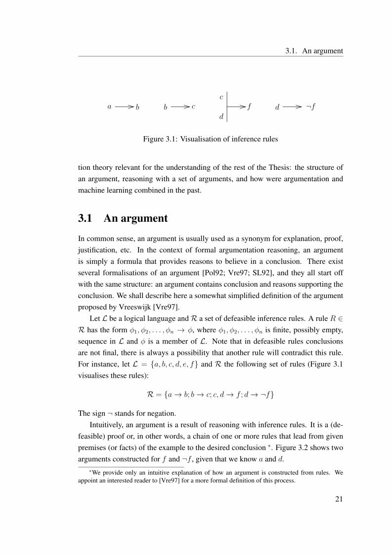
Figure 3.1: Visualisation of inference rules
tion theory relevant for the understanding of the rest of the Thesis: the structure ofan argument, reasoning with a set of arguments, and how were argumentation andmachine learning combined in the past.
3.1 An argument
In common sense, an argument is usually used as a synonym for explanation, proof,justification, etc. In the context of formal argumentation reasoning, an argumentis simply a formula that provides reasons to believe in a conclusion. There existseveral formalisations of an argument [Pol92; Vre97; SL92], and they all start offwith the same structure: an argument contains conclusion and reasons supporting theconclusion. We shall describe here a somewhat simplified definition of the argumentproposed by Vreeswijk [Vre97].
Let L be a logical language andR a set of defeasible inference rules. A rule R ∈R has the form φ1, φ2, . . . , φn → φ, where φ1, φ2, . . . , φn is finite, possibly empty,sequence in L and φ is a member of L. Note that in defeasible rules conclusionsare not final, there is always a possibility that another rule will contradict this rule.For instance, let L = {a, b, c, d, e, f} and R the following set of rules (Figure 3.1visualises these rules):
R = {a→ b; b→ c; c, d→ f ; d→ ¬f}
The sign ¬ stands for negation.Intuitively, an argument is a result of reasoning with inference rules. It is a (de-
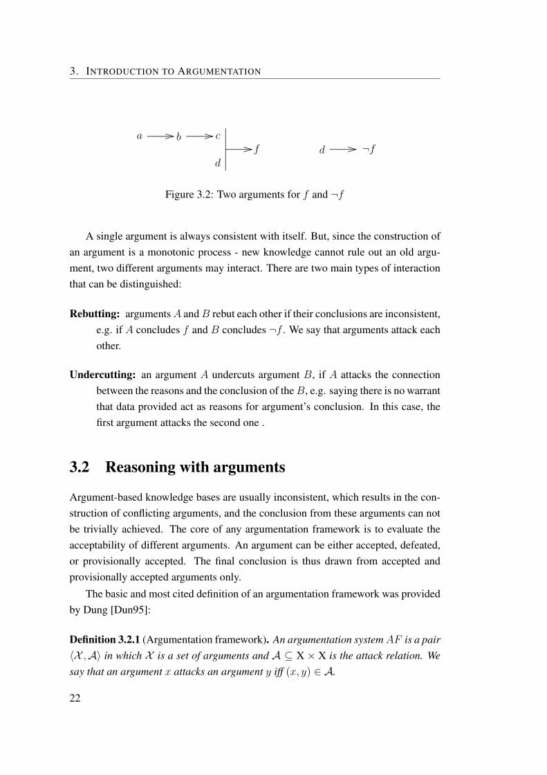
feasible) proof or, in other words, a chain of one or more rules that lead from givenpremises (or facts) of the example to the desired conclusion ∗. Figure 3.2 shows twoarguments constructed for f and ¬f , given that we know a and d.
∗We provide only an intuitive explanation of how an argument is constructed from rules. Weappoint an interested reader to [Vre97] for a more formal definition of this process.
21
3. INTRODUCTION TO ARGUMENTATION
a b.....................................................................................................................
. c.....................................................................................................................
.
d
f
..................................................................................................................
.....................................................................................................................
.
d ¬f.....................................................................................................................
.
Figure 3.2: Two arguments for f and ¬f
A single argument is always consistent with itself. But, since the construction ofan argument is a monotonic process - new knowledge cannot rule out an old argu-ment, two different arguments may interact. There are two main types of interactionthat can be distinguished:
Rebutting: argumentsA andB rebut each other if their conclusions are inconsistent,e.g. if A concludes f and B concludes ¬f . We say that arguments attack eachother.
Undercutting: an argument A undercuts argument B, if A attacks the connectionbetween the reasons and the conclusion of theB, e.g. saying there is no warrantthat data provided act as reasons for argument’s conclusion. In this case, thefirst argument attacks the second one .
3.2 Reasoning with arguments
Argument-based knowledge bases are usually inconsistent, which results in the con-struction of conflicting arguments, and the conclusion from these arguments can notbe trivially achieved. The core of any argumentation framework is to evaluate theacceptability of different arguments. An argument can be either accepted, defeated,or provisionally accepted. The final conclusion is thus drawn from accepted andprovisionally accepted arguments only.
The basic and most cited definition of an argumentation framework was providedby Dung [Dun95]:
Definition 3.2.1 (Argumentation framework). An argumentation systemAF is a pair〈X ,A〉 in which X is a set of arguments and A ⊆ X × X is the attack relation. Wesay that an argument x attacks an argument y iff (x, y) ∈ A.
22
3.2. Reasoning with arguments
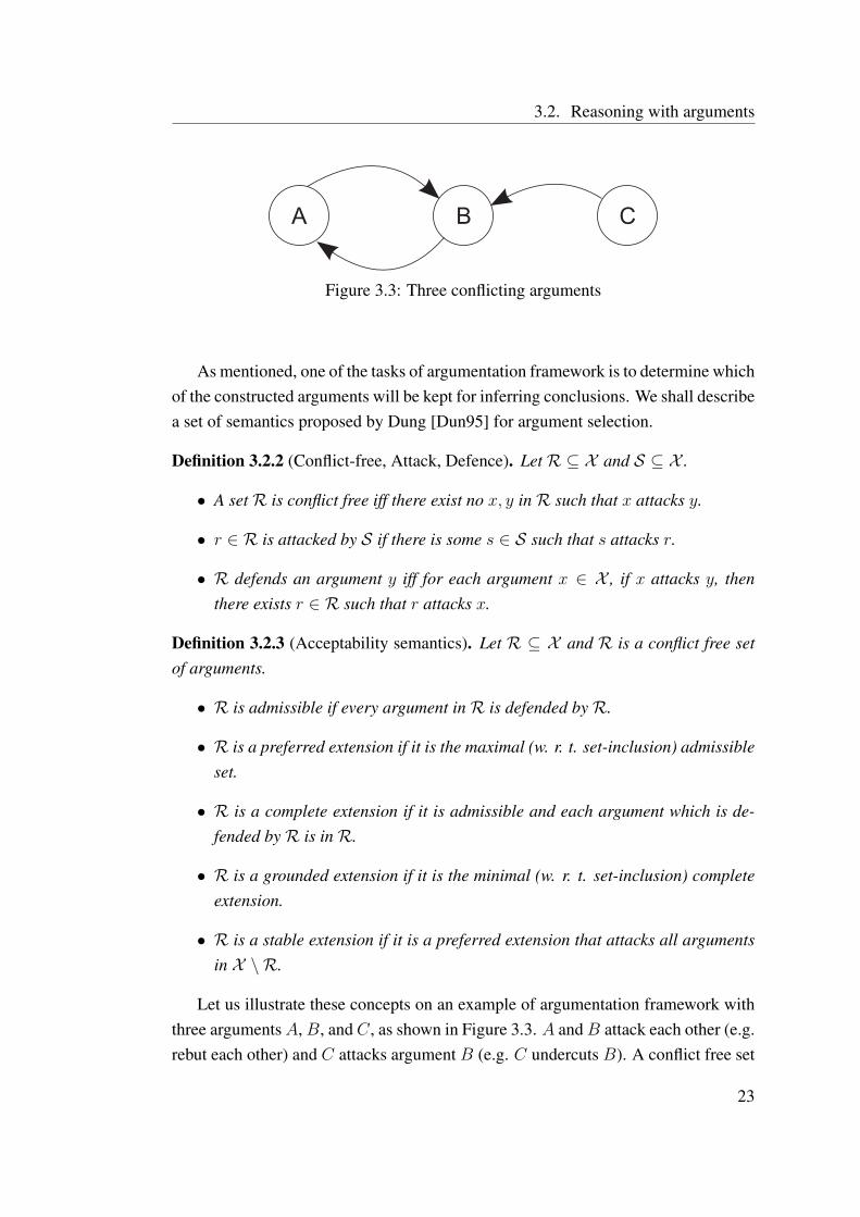
Figure 3.3: Three conflicting arguments
As mentioned, one of the tasks of argumentation framework is to determine whichof the constructed arguments will be kept for inferring conclusions. We shall describea set of semantics proposed by Dung [Dun95] for argument selection.
Definition 3.2.2 (Conflict-free, Attack, Defence). LetR ⊆ X and S ⊆ X .
• A setR is conflict free iff there exist no x, y inR such that x attacks y.
• r ∈ R is attacked by S if there is some s ∈ S such that s attacks r.
• R defends an argument y iff for each argument x ∈ X , if x attacks y, thenthere exists r ∈ R such that r attacks x.
Definition 3.2.3 (Acceptability semantics). Let R ⊆ X and R is a conflict free setof arguments.
• R is admissible if every argument inR is defended byR.
• R is a preferred extension if it is the maximal (w. r. t. set-inclusion) admissibleset.
• R is a complete extension if it is admissible and each argument which is de-fended byR is inR.
• R is a grounded extension if it is the minimal (w. r. t. set-inclusion) completeextension.
• R is a stable extension if it is a preferred extension that attacks all argumentsin X \ R.
Let us illustrate these concepts on an example of argumentation framework withthree argumentsA,B, and C, as shown in Figure 3.3. A andB attack each other (e.g.rebut each other) and C attacks argument B (e.g. C undercuts B). A conflict free set
23
3. INTRODUCTION TO ARGUMENTATION
of arguments is any set, where arguments do not attack each other, e.g. {A,C}. Theset {A,C} defends argument A, since it attacks B, which attacks A. The sets {A},{C}, and {A,C} are admissible, as they all defend themselves. On the other hand,the set {B} is not admissible, because it does not defend itself against the attack ofC. Intuitively, admissible sets are sets of arguments that can defend themselves, or inother words, the set is self-sufficient with respect to defense. Note that the empty setof arguments ∅ is also admissible. The only preferred extension of this argumentationframework is therefore {A,C} (the largest admissible set), and likewise, {A,C} isthe only complete, grounded, and stable extension.
3.3 Argumentation and machine learning
The idea of combining ML and argumentation is not completely new. However, therehave only been a few attempts in this direction. Most of them focused on the useof machine learning to build arguments that can be later used in the argumentationprocess, most notably in the law domain [AR03; BA03]. Gomez and Chesnevar sug-gested in their report [GC04a] several ideas of combining machine learning methodsand argumentation. Moreover, these two authors also developed an approach wherethey used argumentation as a method to improve performance of a neural network[GC04b]. Their method is applied after the actual learning is already finished. Clark[Cla88] proposed the use of arguments to constrain generalization. However, he usedarguments as a special kind of background knowledge that applied to the whole do-main, whereas in this Thesis arguments apply to individual examples.
24
Part II
Argument Based Machine Learningand the ABCN2 Algorithm
25


Chapter 4
Argument Based Machine Learning
In Chapter 2, we showed the difference between various approaches to selecting agood hypothesis that will perform well on unseen examples. One of the possiblesolutions was to constrain search with given prior knowledge - the knowledge aboutthe learning domain. The critical problem of this approach is the difficulty that ex-perts face when they try to articulate their global domain knowledge. Argumentation,which was introduced in the previous chapter, is an approach that allows experts elicittheir knowledge in a more natural way, by allowing the use of their “local” knowl-edge of specific situations, perhaps only valid for these situations. Therefore, we canexpect that the combination of argumentation and machine learning is the one thatshould bring the most benefits.
In this chapter, we will lay out the core idea of Argument Based Machine Learn-ing (ABML), a combination of machine learning and argumentation. We commencewith an illustrating example that should give a quick and intuitive explanation of whatABML is. Based on the given example, we enumerate and explain several expectedmotivations for learning from arguments. In the third section, ABML is formallydefined, and in fourth some general guidelines for implementing ABML methods aregiven. The principles described in this chapter are then used to develop an actual rulelearning algorithm, which is described in the following chapter.
27
4. ARGUMENT BASED MACHINE LEARNING
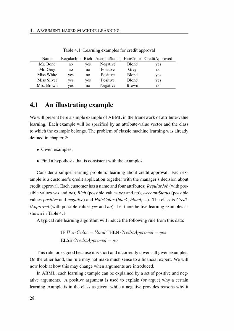
Table 4.1: Learning examples for credit approval
Name RegularJob Rich AccountStatus HairColor CreditApprovedMr. Bond no yes Negative Blond yesMr. Grey no no Positive Grey no
Miss White yes no Positive Blond yesMiss Silver yes yes Positive Blond yesMrs. Brown yes no Negative Brown no
4.1 An illustrating example
We will present here a simple example of ABML in the framework of attribute-valuelearning. Each example will be specified by an attribute-value vector and the classto which the example belongs. The problem of classic machine learning was alreadydefined in chapter 2:
• Given examples;
• Find a hypothesis that is consistent with the examples.
Consider a simple learning problem: learning about credit approval. Each ex-ample is a customer’s credit application together with the manager’s decision aboutcredit approval. Each customer has a name and four attributes: RegularJob (with pos-sible values yes and no), Rich (possible values yes and no), AccountStatus (possiblevalues positive and negative) and HairColor (black, blond, ...). The class is Credi-tApproved (with possible values yes and no). Let there be five learning examples asshown in Table 4.1.
A typical rule learning algorithm will induce the following rule from this data:
IF HairColor = blond THEN CreditApproved = yes
ELSE CreditApproved = no
This rule looks good because it is short and it correctly covers all given examples.On the other hand, the rule may not make much sense to a financial expert. We willnow look at how this may change when arguments are introduced.
In ABML, each learning example can be explained by a set of positive and neg-ative arguments. A positive argument is used to explain (or argue) why a certainlearning example is in the class as given, while a negative provides reasons why it
28
4.2. Motivation
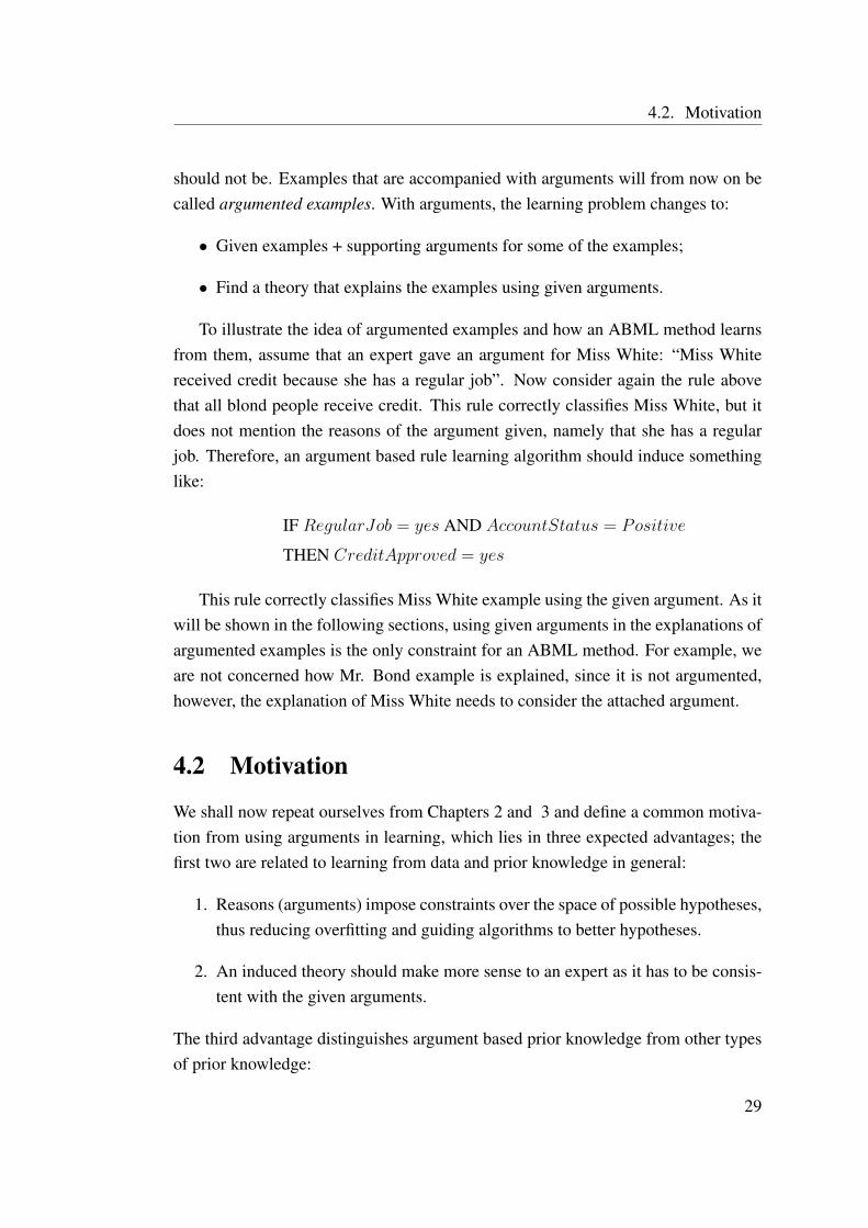
should not be. Examples that are accompanied with arguments will from now on becalled argumented examples. With arguments, the learning problem changes to:
• Given examples + supporting arguments for some of the examples;
• Find a theory that explains the examples using given arguments.
To illustrate the idea of argumented examples and how an ABML method learnsfrom them, assume that an expert gave an argument for Miss White: “Miss Whitereceived credit because she has a regular job”. Now consider again the rule abovethat all blond people receive credit. This rule correctly classifies Miss White, but itdoes not mention the reasons of the argument given, namely that she has a regularjob. Therefore, an argument based rule learning algorithm should induce somethinglike:
IF RegularJob = yes AND AccountStatus = Positive
THEN CreditApproved = yes
This rule correctly classifies Miss White example using the given argument. As itwill be shown in the following sections, using given arguments in the explanations ofargumented examples is the only constraint for an ABML method. For example, weare not concerned how Mr. Bond example is explained, since it is not argumented,however, the explanation of Miss White needs to consider the attached argument.
4.2 Motivation
We shall now repeat ourselves from Chapters 2 and 3 and define a common motiva-tion from using arguments in learning, which lies in three expected advantages; thefirst two are related to learning from data and prior knowledge in general:
1. Reasons (arguments) impose constraints over the space of possible hypotheses,thus reducing overfitting and guiding algorithms to better hypotheses.
2. An induced theory should make more sense to an expert as it has to be consis-tent with the given arguments.
The third advantage distinguishes argument based prior knowledge from other typesof prior knowledge:
29
4. ARGUMENT BASED MACHINE LEARNING
3. An argument focuses on a single learning example only, which allows the ex-perts to elicit their specific example-based knowledge. This reduces the knowl-edge acquisition bottleneck that experts face when providing “classical” gen-eral domain knowledge.
Regarding advantage 1, by using arguments, the computational complexity asso-ciated with search in the hypothesis space can be reduced considerably, and enablefaster and more efficient induction of theories. As thoroughly explained in chapter2, the reduced number of possible hypotheses decreases chances that the best hy-pothesis found is not the true best one, but only an artifact of luck. Moreover, if thelearning algorithm heuristically searches the hypotheses space, a reasonable reduc-tion of space that still contains the best hypothesis will only decrease the probabilitythat the algorithm stops in a local maxima, instead in the global one.
Regarding advantage 2, there are many possible hypotheses that, from the per-spective of a machine learning method, explain the given examples sufficiently well.But some of those hypotheses can be incomprehensible to experts. Using argumentsshould lead to hypotheses that explain given examples in similar terms to those usedby the expert, and correspond to the actual justifications.
The third (3) advantage was already greatly explained in the Argumentation Chap-ter 3. Argumentation has shown to be useful for knowledge elicitation, as it enablesthe knowledge engineer to focus at one case at a time. Similarly, in ABML, the ex-perts need to provide knowledge relating to the specific learning example only, whichcould be valid only for this chosen example rather for the whole domain. As we willshow later, the domain expert needs to explain only some of the learning examples.
4.3 Formal definition of argument based machinelearning
In Chapter 2, we formulated the machine learning problem as a constraint satisfactionproblem. The problem was stated as: given descriptions De and classifications Ce ofeach learning example e, find a hypothesis H that satisfies the constraint:
∀e,H ∧De ` Ce (4.1)
In ABML, a learning example is annotated by a set of arguments. In the mostgeneral case, e.g. if different domain experts would argue about this example, there
30

4.3. Formal definition of argument based machine learning
will be also conflicts between these arguments. As described in section 3.2, a set ofarguments with corresponding attacks between these arguments represent an argu-mentation framework.
Definition 4.3.1 (Argumented Example). An argumented example is a learning ex-ample annotated by an argumentation framework:
• De is a conjunction of example e descriptions,
• Ce is the example e’s classification, and
• AFe is the argumentation framework appended to the learning example e.
An argument in AFe can either support classification Ce (a positive argument) orit can support the negated value of classification ¬Ce (a negative argument).
Definition 4.3.2 (Positive Argument, Negative Argument). Let R be a conjunctionof reasons.
• A positive argument specifies reasons in favour of classification (using wordbecause): Ce because R
• A negative argument specifies reasons against the given classification (usingword despite): Ce despite R
A reason can be any basic property specified in the example’s descriptions. Forexample, having regular job was used as a reason in the argument for Miss White,which was the only reason in that case, although a typical argument uses more thanone reason. The positive argument was:
Miss White received credit because she has a regular job.
The conclusion of this argument is “Miss White received credit”, which is the actualclass of this example, and the reason is “she has a regular job”. An example of anegative argument could be:
“Miss White received credit despite she is not rich”
Using the notation of arguments described in the previous chapter, a positiveargument would be written as R → Ce, meaning that class Ce can be defeasiblyinferred from given reasons. Similarly, the reasons of a negative argument imply theopposite class; R→ ¬Ce. As the conclusions of positive and negative arguments areexactly the opposite, positive and negative arguments attack each other.
31

4. ARGUMENT BASED MACHINE LEARNING
Definition 4.3.3 (Attacks between arguments). There are three different types of at-tack between a positive argument Ap and a negative argument An; they can mutuallyattack each other, or only Ap attacks An, or only An attacks Ap. Two positive ortwo negative arguments can not be conflicting. Let Ap be Rp → Ce and An beRn → ¬Ce.
• Ap attacks An and An does not attack Ap if Rp |= Rn, i.e. negative reasonscan be logically inferred from positive reasons.
• An attacks Ap and Ap does not attack An if Rn |= Rp.
• An and Ap mutually attack each other if Rn = Rp or ¬(Rp |= Rn) ∧ ¬(Rn |=Rp)
In the first two types of attacks one argument undercuts the other, while in thethird type arguments rebut each other. The set of positive and negative argumentstogether with attacks among them present an argumentation framework attached to alearning example.
As we mentioned within the motivating example, the learning problem using ar-guments changes to:
• Given examples + supporting arguments for some of the examples
• Find a theory that explains the examples using given arguments
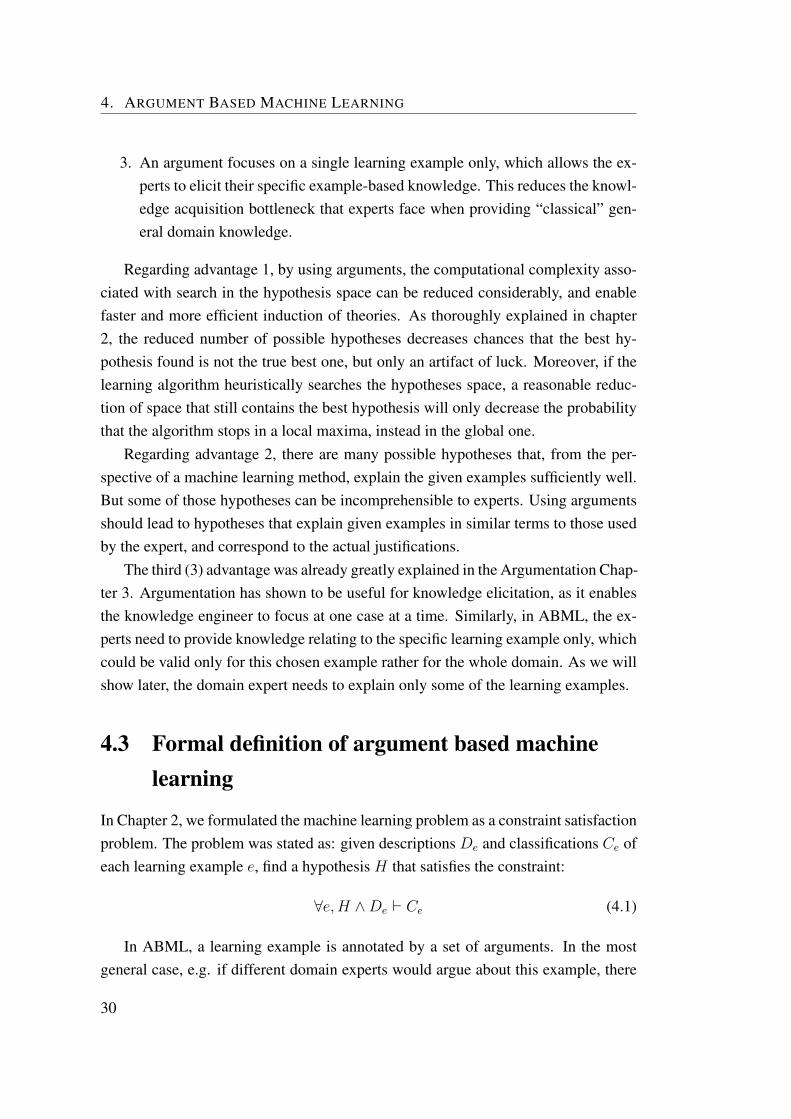
In logical terms, a theory explains an example using given arguments, if the rea-sons of given arguments are mentioned during the derivation of the example. Thedefinition of argument-based machine learning therefore needs to use an additionalconstraint in the derivation process:
∀e,H ∧De `AFe Ce (4.2)
To help us define the argument-based derivation `AF , we need to introduce a newfunctionR over a set of arguments S:
R(S) = {r|∃a ∈ S; r ∈ Reasons(a)} (4.3)
The functionR(S) returns the set of all reasons used in arguments in S.
32

4.3. Formal definition of argument based machine learning
Figure 4.1: An illustration of a proof tree of an argumented example. The proof men-tions one positive admissible set, and does not mention any of the negative admissiblesets.
Definition 4.3.4 (Argument-based derivation). Let AF be an argumentation frame-work, let P = {P1, . . . ,Pk} be all nonempty admissible sets of positive argumentsand N = {N1, . . . ,Nl} all nonempty admissible sets of negative arguments in AF .Then, B is argument-based derived from A with respect to AF , written as A `AF B,if:
• A ` B, and
• each possible derivation (in a given deduction system) of B given A mentionsat least one positive admissible set Pi, and
• each possible derivation of B given A does not mention any of the negativeadmissible sets.
A derivation mentions a set of arguments S if all reasonsR(S) are mentioned withinthe derivation process.
Therefore, in the case of ABML, all possible proofs of classifications Ce fromthe induced hypothesis H and descriptions De should mention at least one of theadmissible sets of positive arguments and none of the admissible sets with negativearguments. Remember that an admissible set is a set of not defeated (they can defend
33

4. ARGUMENT BASED MACHINE LEARNING
themselves) and not conflicting (no attacks between arguments) arguments. Figure4.1 illustrates a proof tree that considers constraints by arguments.
Example 4.3.5. Consider again Miss White from our illustrating example. Her creditapproval was explained by a single positive argument p: “Miss White received creditbecause she has a regular job”. Therefore, the only admissible set of argumentscontains p only; P = {{p}}. Since there are no negative arguments, there are nonegative admissible sets. In this case, the argument-constrained derivation of MissWhite classification should mention reason of p, namely “she has a regular job”.
Example 4.3.6. Let us expand the attribute space of our illustrating learning prob-lem 4.1 with a OwnsHouse feature (whether the person owns a house or not) andassume that Miss White owns a house. Then, an expert could give the following fourarguments (2 positive and 2 negative) to Miss White:
p1; Miss White received credit because she has a regular job.
p2; Miss White received credit because she owns a house.
n1; Miss White received credit despite she is not rich.
n2; Miss White received credit despite she is blond.
There are three positive admissible sets {{p1}, {p2}, {p1, p2}} and three negativeadmissible sets {{n1}, {n2}, {n1, n2}}. Therefore, the proof of Miss White exam-ple should contain reasons of at least one admissible sets (RegularJob=yes, Own-sHouse=yes, or both) and should not contain any reasons of negative examples(Rich=no, HairColor=blond).
Example 4.3.7. Let us further expand the feature space with CreditAmount (amountof money asked for) and HouseValue (value of applicant’s house on the real-estatemarket). Miss White asked for a credit amount of 200 thousand EUR (CreditA-mount=200), while her house could be sold for 150 thousand EUR (HouseValue =150). The domain expert could add a new negative argument n3: “Miss White re-ceived credit despite that credit amount is higher than the value of her house”. Thereasons of this argument imply that she owns a house (ownsHouse=yes), thereforethis argument attacks p2, while p2 does not attack it back (owning a house does notimply its price). Figure 4.2 visualises attacks between the five arguments. In this
34
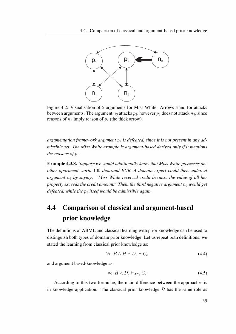
4.4. Comparison of classical and argument-based prior knowledge
Figure 4.2: Visualisation of 5 arguments for Miss White. Arrows stand for attacksbetween arguments. The argument n3 attacks p2, however p2 does not attack n3, sincereasons of n3 imply reason of p2 (the thick arrow).
argumentation framework argument p2 is defeated, since it is not present in any ad-missible set. The Miss White example is argument-based derived only if it mentionsthe reasons of p1.
Example 4.3.8. Suppose we would additionally know that Miss White possesses an-other apartment worth 100 thousand EUR. A domain expert could then undercutargument n3 by saying: “Miss White received credit because the value of all herproperty exceeds the credit amount.” Then, the third negative argument n3 would getdefeated, while the p1 itself would be admissible again.
4.4 Comparison of classical and argument-basedprior knowledge
The definitions of ABML and classical learning with prior knowledge can be used todistinguish both types of domain prior knowledge. Let us repeat both definitions; westated the learning from classical prior knowledge as:
∀e, B ∧H ∧De ` Ce (4.4)
and argument based-knowledge as:
∀e,H ∧De `AFe Ce (4.5)
According to this two formulae, the main difference between the approaches isin knowledge application. The classical prior knowledge B has the same role as
35

4. ARGUMENT BASED MACHINE LEARNING
the induced hypothesis, it is used in the derivation of all learning examples. On theother hand, argument-based knowledge has to be mentioned within the derivation ofargumented examples only. It is desirable that arguments would be mentioned alsoin the explanations of other examples, to use experts knowledge as often as possible,however this is not required by the method. Naturally, argument-based approach andclassical prior knowledge could be used together:
∀e, B ∧H ∧De `AFe Ce (4.6)
Argument-based approach to machine learning can be easily misunderstood as aspecial kind of explanation-based learning. Let us recall the definition of explanation-based learning:
∀e,H ∧De ` Ce (4.7)
B ` H
Perhaps it is not best visible from the formulae, but approaches do share some simi-larities. In explanation-based learning, prior knowledge is first used to explain learn-ing examples. It is assumed that search for these proofs or explanations is time-consuming, so it might make sense to generalise these “local” proofs and store themfor faster future processing of similar examples. The generalisation in the EBG senseis simply replacing facts in specific proofs with variables that do not change the va-lidity of the proof. In ABML, arguments represent a sort of partial “local” proofs,and an ABML method also generalises these proofs. However, the proofs in ABMLare not complete and the generalisation step requires inductive reasoning, while inexplanation-based learning it does not. Therefore, the main difference between bothapproaches is that the hypothesis in explanation-based learning can be logically in-ferred from prior knowledge - there is no inductive learning whatsoever, while inABML the hypothesis can can not be inferred from B.
4.5 Guidelines for building argument based machinelearning methods
The first task in the construction of an ABML method is to select the base method,which will be later extended to learn from argumented examples. Here we need toconsider that arguments lead to hypotheses that are more comprehensible to domain
36

4.5. Guidelines for building argument based machine learning methods
experts. This can only be demonstrated if the hypothesis language allows humanexplanations, e.g. decision trees or logistic regression. We believe that the bestcandidates for the base method in ABML are symbolic methods, where hypothesesare encoded with a set of human readable symbols. However, there is no true obstaclenot to use arguments also in other methods, e.g. instance-based methods like kernelor k-nearest-neighbour (KNN) methods, but we will not be able to easily spot theincreased understandability in hypotheses achieved with the help of arguments.
After we selected a machine learning method, we need to answer the followingquestions:
1. What is the language for representing arguments?
2. What do we mean by “reasons should be mentioned in the derivation of ex-amples” for the selected learning method? What actually is argument-basedderivation for the selected method?
3. How can we effectively guide learning towards hypotheses consistent with ar-guments?
4. How is statistical error considered in argumented and non-argumented exam-ples?
The formal language for reasons in arguments should be the same as the languagedefining the hypothesis space. For example, if the hypothesis is a logical program,then the reasons should be logical sentences. This enables direct reflection of ar-guments in the induced hypothesis - the reasons of arguments construct part of thehypothesis. It greatly helps a domain expert to position his or her knowledge andobserve the new, automatically obtained, knowledge in the hypothesis. The second(2) question is related to the reasoning with induced hypothesis and the third (3) isrelated to the search space and how can it be effectively constrained. The fourth(4) question is not crucial for the method to work (in some methods its solution ispractically impossible), but it can increase the quality of induction. The argumentsdifferently constrain different parts of the hypotheses space. In some cases, wherearguments are very specific, the induction algorithm will not have much generalisa-tion to do, and there we can expect low to no overfitting. However, the hypothesisspace related to the non-argumented examples can be less constrained, whereas wecan expect to deal with a higher amount of overfitting.
37
4. ARGUMENT BASED MACHINE LEARNING
In the case of the ABCN2 algorithm, which is going to be described in the fol-lowing chapters, we shall thoroughly study and provide answers to all four questions.But first, we will look at two short examples to show ideas for transforming two ma-chine learning methods, inductive logic programming and logistic regression, to theirargument-based counterparts, which are meant to provide the reader with a more gen-eral understanding of these questions. The answer to the fourth question is relativelyhard and not necessary for understanding the basic principles, hence it will be omittedin these two examples.
4.5.1 Argument based inductive logic programming
Inductive Logic Programming (ILP) learns hypotheses from background knowledgeand descriptions of examples provided in first-order logic sentences. Each example isclassified either as positive or negative. The problem is to find such a hypothesis that(together with background knowledge) proves all positive examples and no negativeones.
According to our guideline, we will code the reasons of arguments in first-orderlogic. As usually, an argument presents a link between example’s descriptions and itsclass value. However, in ILP a reason does not need to be explicitly part of descrip-tion of examples, but can mention a reason that can be inferred from descriptionsand background knowledge. For example, we could have the following rule in back-ground knowledge (using the syntax of Prolog):
union_member(X) :- % X is a member of a labor union
regular_job(X),
not rich(X).
The argument for Miss White could then change to “Miss White received credit be-cause she is a member of a labor union.” Another type of arguments in ILP come fromthe fact that ILP is particularly suitable for problems where learning examples are re-lated to each other (e.g. graphs). This means that the reasons of arguments can alsocontain relations between examples or even contain the descriptions of some other re-lated example. To illustrate this specific type of reasons, consider that we could addmarried relation to our credit example, where married(person1, person2) meansthat person1 and person2 are married. After adding a fact to the domain:
married(mr_Bond, miss_White).
38

4.5. Guidelines for building argument based machine learning methods
the expert is entitled to add the following arguments to the Miss White example:“Miss White received credit because she is married to Mr. Bond.” or “Miss Whitereceived credit because Mr. Bond is rich.”
Since the usual problem statement of ILP is very similar to our definition ofgeneral machine learning, there should be no problems with the understanding ofargument-based derivation concept. A hypothesis in AB-ILP is consistent with thegiven arguments if the proof tree of the learning example contains reasons of thegiven arguments. In our Miss White example, we require that factmarried(mr Bond,miss White) or fact rich(mr Bond) is mentioned in the pro-cedure, respectively for the last two example arguments.
The last question is how to efficiently search through a set of hypotheses consis-tent with arguments. Using a standard ILP algorithm and simply disregarding incon-sistent hypotheses would work in theory, however it could be very slow, especiallyif an argument would mention facts that are “far” away from the argumented exam-ple. For a possible improvement, we could consider facts as nodes in graph, whilerelations and rules would connect these nodes. Then, an algorithm for finding theshortest path, e.g. Dijkstra’s algorithm, could be used to connect the facts mentionedin the reasons of an argument with the facts in the description of the example. Thesealgorithms are relatively fast. The complete path from reasons to facts of examplewould then be used to form the basic structure of the induced hypothesis, while ILPwould only need to induce additional required conditions.
4.5.2 Argument based logistic regression
Logistic regression is a linear method for classification. It is suited for domains withcontinuous domain descriptors (attributes) X = {x1, . . . , xn} and a binary class y.Given class and attributes, logistic regression maximises log-likelihood by optimisingparameters in the formula:
p(y|X) =1
1 + e−f(X)(4.8)
f(X) = a0 + a1x1 + a2x2 + . . .+ anxn
This formula is thus used to calculate the probability of class y given description Xof an example.
The usual interpretation of logistic regression formula is in terms of attributechanges, for example: if the coefficient ai is positive, then the probability of classy for a particular example would increase if the value of xi of this example would
39
4. ARGUMENT BASED MACHINE LEARNING
increase, while all other attribute values would stay the same. The reasons of an argu-ment in argument-based logistic regression should thus also be given in a qualitativesense. Consider an example with the actual values:
(x1 = 0.5, x2 = 0.8, . . . , xi = 6, . . . , xn = −4.3), y = 1
A possible argument for this example could be: “The value of y equals 1 because thevalue of xi is high”. This argument can be interpreted then as: the higher is the valueof xi, the larger is the probability P (y = 1).
The argument can be easily converted into a constraint on the induction of lo-gistic models. In the example above, the argument suggests that the value of theai parameter is likely to be positive. One way to assure such constraint is to usenon-symmetric bias in bayesian logistic regression [GLM07] that would prefer eitherpositive or negative values of a parameter. Alternatively, we could use any form ofstrictly constrained logistic regression [VR02], where the values of the parameterscan be limited to be either positive or negative.
Using constraints in logistic regression will force the change of parameters, whichwill reflect on the classification of all examples. Such constraints are not according tothe idea of argument based learning; the positiveness of ai parameter is required onlyin classification of this particular example and not for the whole learning domain.However, this approach is still acceptable, as long as this change does not worsenthe prediction on other learning examples. Otherwise, a solution would be a methodthat somehow divides the example space and learns a logistic model in each of thesubspaces. An example of a such method is Logistic Model Tree [LHF03].
40
Chapter 5
Argument Based Rule Learning(ABCN2)
In this chapter, we will describe argument based CN2 (ABCN2 for short), a methodfor learning classification rules from argumented examples. ABCN2 is an extensionof the well-known rule learning algorithm of Clark and Niblett ([CB91]). The workdescribed here bases on our earlier papers on the idea of AB-enhancement of CN2([MvB06; MvB07].
We will begin with a definition of argumented examples accepted by ABCN2. Af-ter, we shall look at the algorithm ABCN2 itself, describe the concept of AB-coveringand propose some changes of the basic algorithm to improve its time efficiency. Thelast section of this chapter gives some details of the actual implemented product.
There is one critical question though that we need to answer before we move tothe description of the method: Why have we chosen rule learning, and why partic-ularly CN2, as the basis of our argument-based method? The question is perfectlyvalid, as there are various standard ML techniques that could be extended into anargument-based variant. One of the reasons is the structure of a single argument;human-based arguments often have a form similar to propositional rules, where thereason of an argument is a conjunction of premises (see chapter 3). Therefore, follow-ing our guideline that learned knowledge should be represented the same as existingknowledge, we believe that rule learning is the most appropriate machine learningapproach to be used with argumentation. CN2 was selected since it is the most com-monly used and well undestood algorithm for induction of unordered rules, where
41
5. ARGUMENT BASED RULE LEARNING (ABCN2)
by “unordered” we mean that classification from rules considers all applicable rulesfor the example and not just the first that triggers. We also extended CN2 in manyaspects (evaluation of rules, covering strategy, classification from rule), which bringsCN2 on a similar level, in terms of accuracy, with other currently popular machinelearning methods.
5.1 Argumented examples
A learning example E in the usual form accepted by CN2 is a pair (A,C), where Ais an attribute-value vector, and C is a class value. An attribute can be either discrete(finite unordered set of values) or continuous. In addition to such examples, ABCN2also accepts argumented examples. An argumented example AE is a triple of theform:
AE = (A, C, Arguments)
As usual, A is an attribute-value vector and C is a class value. Arguments is a set ofarguments Arg1, . . . , Argn, where an argument Argi has one of the following forms:
C because Reasons
or
C despite Reasons
The former specifies a positive argument (speaks for the given class value), while thelatter specifies a negative argument (speaks against the class value). Reasons is aconjunction of reasons r1, . . . , rn,
Reasons = r1 ∧ r2 ∧ . . . ∧ rn
where each of the reasons ri can be in one of five possible forms. In the explanationof these forms below we assume that ri is a part of a positive argument; for negativearguments, the explanations are exactly the opposite. The five forms of reasons are:
• X = xi means that value xi of attribute X is the reason why example is in theclass as given. This is the only allowed form for discrete attributes.
• X > xi (orX >= xi) means that the value of attribute X of example beinggreater than (greater or equal to) xi is the reason for class value.
42
5.1. Argumented examples
• X < xi (orX <= xi) the opposite to X > xi (X >= xi).
• X > (orX >=) “X is high”; similar to X > xi (X >= xi), just that we donot know the threshold value and it has to be found by ABCN2 automatically.Such an argument says that the value of X of the example is high enough forthe example to be in the class as given.
• X < (orX <=); “X is low”, the opposite of X > (X >=).
We shall now revisit again our key example Miss White from Table 4.1. The pos-itive argument said: “Miss White received the credit because she has a regular job”,while one of the negative arguments was: “Miss White received the credit despiteshe is not rich”. The Miss White example would in our syntax be written as:
((RegularJob = yes, Rich = no,AccountStatus = positive,HairColor =
blond),CreditApproved = yes,
{CreditApproved = yes because RegularJob = yes,CreditApproved = yes despite Rich = no}).
Arguments given to examples additionally constrain rules covering this example.Remember that in CN2, rules have the form:
IF Complex THEN Class
where Complex is the conjunction of simple conditions, called selectors. Usually,a selector specifies the value of an attribute, for example HairColor = blond or athreshold on an attribute value, for example Salary > 5000. A rule for our creditapproval domain can be:
IF rich = no AND HairColor = blond
THEN CreditApproved = yes
The condition part of the rule is satisfied by the attribute values of Miss Whiteexample, so we say that this rule covers this example.
A rule R is consistent with an argument ”C because Reasons” (or ”C despiteReasons”), if for all reasons ri of Reasons it is true that:
43
5. ARGUMENT BASED RULE LEARNING (ABCN2)
1. If the reason ri is in one of forms: “X = xi” or “X > xi” or “X < xi”(“X >= xi” or “X <= xi”), then exactly the same selector needs to be presentin the complex of the rule R.
2. If the reason ri has the form “X >” (or “X <”, “X <=”, “X >=”), thenthe complex of the rule R needs to contain a selector “X > xi” (or “X <
xi”, “X >= xi”, “X <= xi”). The threshold value xi does not matter forconsistency.
Having the form of arguments defined, we need to implement the concept ofargument-constrained derivation in argument based rule learning. To this end, wewill refine the definition of covering relation. In the standard definition [CN89], arule covers an example if the condition part of the rule is true for this example. Inargument based rule learning, this definition is modified to: A rule R AB-covers anargumented example E if all of the points below hold:
1. All conditions in R are true for E (same as in CN2),
2. R is consistent with at least one positive argument of E, and
3. R is not consistent with any of negative arguments of E.
The AB-covers relation corresponds to the argument-constrained derivation definedwithin the general ABML framework. The complete inference from a propositionalrule to an example has only one step: from conditions of the rule to the facts of theexample. If arguments have to be mentioned in the explanation of the example, thenthe reasons of arguments need to be a part of the complex. Since arguments in rulelearning can not undercut other arguments (we can assume without loss that under-cutted arguments are removed prior to learning), each argument itself is admissible,which allows the use of arguments instead of admissible sets in points 2 and 3.
As an illustration of the differences between AB-covering and the usual definitionof covering, consider again the Miss White example with the argument that she re-ceived credit because she has a regular job and despite she is not rich. Now considerfour rules:
R1: IF HairColor = blond THEN CreditApproved = yes
R2: IF Rich = no AND HairColor = blond
THEN CreditApproved = yes
44
5.2. Argument based CN2 algorithm
R3: IF Rich = no AND RegularJob = yes
THEN CreditApproved = yes
R4: IF HairColor = blond AND RegularJob = yes
THEN CreditApproved = yes
All four rules cover the Miss White example and have 100% accuracy on the dataset from Table 4.1. However, Rule 1 does not AB-cover the example, because it isnot consistent with the positive argument. For the same reason, rule 2 does not AB-cover the Miss White example, but this rule fails also because it is consistent withthe negative argument (Rich = no). Rule 3 also fails due to the negative argument,although it is consistent with the positive argument. The last example AB-covers theMiss White example.
5.2 Argument based CN2 algorithm
The CN2 algorithm [CN89; CB91] consists of a covering algorithm and a searchprocedure that finds individual rules by performing beam search. The covering algo-rithm induces a list of rules that cover all the examples in the learning set. Roughly,the covering algorithm starts by finding a rule, then it removes from the set of learn-ing examples those examples that are covered by this rule, and adds the rule to theset of rules. This process is repeated until all the examples are removed.
There are two versions of CN2: one induces ordered list of rules, and the otherunordered list of rules. Our algorithm is based on the second version of CN2. Inthis case, the covering algorithm consists of two procedures, CN2unordered andCN2ForOneClass. The first procedure iteratively calls the second for all the classesin the domain, while the second induces rules only for the class given. When remov-ing covered examples, only examples of this class are removed [CB91]. Essentially,CN2ForOneClass is a covering algorithm that covers the examples of the given class.
5.2.1 ABCN2: covering algorithm
Remember that in ABML an induced hypothesis must explain argumented exam-ples using given arguments. We showed that a single rule explains an argumentedexample, if the rule AB-covers the example. A hypothesis induced by CN2 is a set ofrules, and there are several different techniques to classify an example from a set ofif-then rules. They all first select the rules that apply for the classifying example, and
45

5. ARGUMENT BASED RULE LEARNING (ABCN2)
Algorithm 5.1 Pseudo code of the original CN2ForOneClass procedure.Procedure CN2ForOneClass(Examples ES, Class T)
Let RULE LIST be an empty list.while ES is not empty do
Let BEST RULE be Find best rule(ES,T)Add BEST RULE to RULE LIST.Remove from ES examples covered by BEST RULE.
end whilereturn RULE LIST
Algorithm 5.2 Covering algorithm of ABCN2 algorithm that learns rules from ex-amples ES for given class T.
Procedure ABCN2ForOneClass(Examples ES, Class T)
Let RULE LIST be an empty list.Let AES be the set of examples in class T that have arguments; AES ⊆ ESDetermine threshold in vague arguments (type X >, etc.)Evaluate arguments (as if they were rules) of examples in AES and sort examplesin AES according to quality of their best argument.while AES is not empty do
Let AE1 be the first example in AES.Let BEST RULE be ABFind best rule(ES,AE1,T)Add BEST RULE to RULE LIST.Remove from AES examples AB-covered by BEST RULE.
end whilefor all RULE in RULE LIST do
Remove from ES examples AB-covered by RULE.end forAdd rules obtained with CN2ForOneClass(ES,T) to RULE LISTreturn RULE LIST
then combine these rules to classify the example. Therefore, to satisfy the ABMLrequirement, there needs to be at least one rule in the set of induced rules that AB-covers this example. This can be achieved relatively simply, by merely replacing thecovering relation in original CN2 with AB-covering.
Replacing the “covers” relation in CN2 with “AB-covers” in ABCN2 ensuresthat both argumented and non-argumented examples are AB-covered. However, inaddition to simply AB-covering all the examples, we would also prefer explainingas many as possible non-argumented examples by arguments given for the argu-
46

5.2. Argument based CN2 algorithm
mented examples. Therefore, we propose a change in the covering algorithm, whereCN2ForOneClass is changed into ABCN2ForOneClass (see Algorithm 5.1 for theoriginal algorithm and in Algorithm 5.2 the new one). The procedure starts by cre-ating an empty list of rules, and makes a separate set AES of argumented examplesonly. Then it looks for “unfinished” arguments - arguments that have some of thereasons “vaguely” specified (X > and X <) and finds the best splits for these rea-sons. Splits are initially set simply to the attribute value of the argumented example;we then iteratively generalise them to achieve the highest quality. Arguments in theexamples AES are then evaluated by the rule evaluation function∗ as if the argumentswere rules of the form
IF reasons of argument THEN claim of argument
The examples in AES are then sorted according to the “goodness” of their best argu-ments.
In the while loop, the procedure induces a rule, using ABFind Best rule, to coverthe first argumented example. ABFind Best rule is a modified beam search proce-dure that accepts examples, an argumented example and a target class, where theresulting rule is guaranteed to AB-cover the given argumented example. This ruleis added to the rule set, and the procedure removes from AES argumented examplesAB-covered by this rule. The removal of all positive examples is not necessary, aseach of the argumented examples differently constrains the search and thus preventsABCN2 from inducing the same rule again. When all argumented examples are cov-ered, all positive examples AB-covered by rules are removed, and the remaining rulesare learned using classical CN2ForOneClass.
5.2.2 ABCN2: search procedure.
Algorithm 5.3 shows the argument-based search procedure. The procedure takesa set of examples to learn from, an argumented example that needs to be AB-coveredby the induced rule, and the target class. In Algorithm 5.3 the underlined parts em-phasize the differences between the original search procedure in CN2 and the AB-search procedure:
Initial value of set STAR is the set of positive arguments of example E. A rule in-duced from an argumented example must AB-cover this example, therefore it
∗The original CN2 algorithm uses Laplacian formula of succession for evaluation of rules. Wewill propose an alternative evaluation in the Chapter 6.
47

5. ARGUMENT BASED RULE LEARNING (ABCN2)
Algorithm 5.3 Algorithm that finds the best rule that AB-covers the argumentedexample E. The “quality” of a complex is evaluated by a user-defined evaluationfunction.
Procedure ABFind Best Rule(Examples ES, Example E, Class T)
Let the set STAR contain reasons of positive arguments of E.Evaluate complexes in STAR (using quality function).Let BEST CPX be the best complex from STAR.Let SELECTORS be the set of all possible selectors that are TRUE for ELet ARG REASONS be the set of all reasons in positive arguments of E (unionof reasons).while STAR is not empty do{Specialize all complexes in STAR as follows}Let NEWSTAR be the set{x ∧ y ‖x ∈ STAR, y ∈ SELECTORS}
Remove from NEWSTAR all complexes that are consistentwith any of negative arguments of E.for every complex Ci in NEWSTAR do
if Ci is statistically significant(ES,T) andquality(Ci) > quality(BEST CPX) thenreplace the current value of BEST CPX by Ci
end ifend forLet STAR be best N complexes from NEWSTAR; N is a user-defined size ofSTAR (usually N=5).Let ABNEWSTAR be such subset of NEWSTAR,
where complexes in ABNEWSTAR contain onlyconditions from ARG REASONS.
Let ABSTAR be best N complexes from ABNEWSTAR.Let STAR be STAR merged with ABSTAR.
end whilereturn rule: ”IF BEST CPX THEN T.´´
will have to contain the reasons of at least one of positive arguments. Theeasiest way to ensure this is to start learning from them.
Specialize with selectors that are satisfied by argumented example. This ensuresthe coverage of the seed example by the induced rule.
Remove all complexes that are consistent with negative arguments. Again, rulesmust AB-cover argumented example, therefore can not be consistent with anyof the negative arguments.
48

5.2. Argument based CN2 algorithm
Let ABSTAR be best N complexes from ABNEWSTAR. Rules that contain onlyconditions that are present in positive arguments are likely to be consistentwith domain knowledge. Thence, these rules are deemed promising, even ifat the moment they are not among first N best rules according to the equalitymeasure.
5.2.3 Time complexity and optimisation
CN2
The complexity of learning a single rule in original CN2 depends on the data setproperties and learner’s settings ([CN89]). Let:
a be the number of all attributes in the given data set,
e number of examples,
s size of star (as set in CN2), and
L maximum allowed length of a rule.
The evaluation of a single rule has time complexity O(e), since it has to sweepthrough all examples to determine which of the examples are covered by the rule andwhich are not. In each specialisation step of CN2, we need to evaluate O(s · a) rules,therefore the complete specialisation takesO(e ·s ·a). Following specialisation, CN2sorts rules by their quality to select the best N in STAR, which has time complexityO((s · a)log(s · a)). Finally, as learning a single rule contains L specialisations, thelearning of a complete rule has time complexity O(L · s · a(e+ log(s · a))).
ABCN2
Learning rules from argumented data is on one hand slower, due to additional checksin AB-cover relation, and faster, as rule learner starts specialising a given argumentand not the empty complex. To estimate the time complexity, we need to define thefollowing new values:
lp is the average length of positive arguments,
np is the average number of positive arguments given to examples,
ln is the average length of negative arguments, and
49
5. ARGUMENT BASED RULE LEARNING (ABCN2)
nn is the average number of negative argument given to examples.
The time complexity of sorting elements in the beam stays the same O((s ·a)log(s · a)). The main difference is in the cover relation, viz., to pick out exam-ples that are covered by a rule. First, a check is needed if the new attribute valueis true for each example, which takes O(e). Then, if the current length of rule is l,we need O(e · np · lp · l) operations to find out whether the rule is consistent with atleast one positive argument, and similarly, O(e · nn · ln · l) for negative arguments.Together, evaluation of a single specialisation requires O(e · (l · (np · lp + nn · ln))).Since learning starts with the positive argument, number of specialisations is reducedto L− lp, therefore the learning of a complete rule takes:
O
(L− lp) · s · a
e · i=L∑i=lp
i · (np · lp + nn · ln)
+ log (s · a)
= O
((L− lp) · s · a
(e ·(L(L+ 1)− lp(lp + 1)
2· (nplp + nnln)
)+ log (s · a)
))Apparently, the term in the middle (np · lp + nn · ln) is the main factor increasing
time complexity of learning rules from arguments. Any increase in argument’s lengthand number of arguments given to examples (positive or negative) will result in anincrease of this factor, and probably also in the increase of overall time complexity.Only the length of positive arguments has an uncertain polarity of influence, for italso effects the complexity positively by reducing the number of specialisations toL− lp.
Speed-ups of ABCN2
The current algorithm ensures that at least one rule will AB-cover each learning ex-ample. The same would be achieved, though, by enforcing a rule to AB-cover onlythe seed example in procedure ABCN2ForOneClass (see Algorithm5.2) and use clas-sical covering instead. In this way, we do not need to check whether a rule is con-sistent with positive arguments, as positive arguments are used in root of the rule.Moreover, consistency with negative arguments has to be checked only for the seedexample and not for others. With the mentioned change, the time complexity of thealgorithm decreases to:
O
((L− lp) · s · a
(e+
L(L+ 1)− lp(lp + 1)
2· nn · ln + log (s · a)
))(5.1)
50

5.2. Argument based CN2 algorithm
The complexity of the algorithm is now significantly reduced. To begin with,the length or number of arguments do not increase time anymore, which favourstherefore to have as many positive arguments as possible. Moreover, the term nn · lnrelated to negative arguments is not multiplied by the number of examples e anymorethat also improves the time efficiency a lot. It is also important that this improvementdoes not change algorithms 5.2 and 5.3, since it only affects the evaluation of rules,particularly determination which examples are covered by rule and which not. Wewill use this speed-up in all our experiments.
5.2.4 Implementation
The ABCN2 algorithm is implemented within the Orange-toolkit [DZ04]. It is in-cluded within the standard distribution of Orange http://www.ailab.si/orange/along with all the necessary documentation.
51

Chapter 6
Extensions of ABCN2
The main issue discussed in this chapter is evaluation of rules in ABCN2. We willshow that the multiple-comparison problem described by [JC00] makes evaluationof rules unavoidably optimistic. The problem is not so acute in standard CN2, sinceall rules are similarly optimistic. However, in the case of ABML, particularly in thecase of ABCN2, rules learned from argumented examples are typically selected fromless candidates than rules induced by a standard rule learning algorithm, and thus thequality of a rule learned from an argumented example is relatively under-estimatedwhen compared to a rule learned from standard CN2.
We shall describe a new method Extreme Value Correction based on ExtremeValue Distributions that takes multiple-comparisons into account. We will begin witha description of a general algorithm and continue with a specific algorithm suited es-pecially for rule learning. We conclude the chapter with a new strategy for rule cov-ering, which is necessary to enable efficient application of Extreme Value Correctionin ABCN2.
6.1 Extreme value correction
Extreme Value Correction (EVC) is a new method presented in this Thesis that cor-rects the optimistic evaluations of constructed hypotheses in machine learning algo-rithms. Most of these algorithms evaluate several hypotheses during learning andchoose the one with the best score. Since these estimates are based on the trainingdata from which the hypotheses themselves were constructed, they are inevitably op-
53
6. EXTENSIONS OF ABCN2
timistic. a decade ago Jensen and Cohen [JC00] did an extensive study of this pathol-ogy. They spotted three main characteristics of learning algorithms contributing tothe optimism of evaluations: attribute selection error, overfitting and oversearching.EVC is a mechanism that aims at solving all three problems.
Overfitting is usually seen as constructing overly complicated and detailed hy-potheses in order to better fit the data. The problem is traditionally dealt with byvarious restrictions on the model language and the search procedure, or by posteriorsimplification of the constructed models.
Overconfidence is related to overfitting; discovered hypotheses, mostly compli-cated, tend to be assigned an exaggerated, overly optimistic probabilities of beingtrue or another related statistics. The reason lies in the way the machine learningalgorithms operate. In the standard use of statistics, the hypotheses are made inadvance and then tested on independent data sets, which gives unbiased estimatesof their true statistical properties. Machine learning constructs hypotheses from thedata and during the induction process implicitly tests them on this same data, whichmakes the estimates unreliable.
As an example, assume that h1, h2, . . . are all possible hypotheses producibleby a certain learning algorithm, and let q1, q2, . . . be their corresponding qualities.The hypotheses can be, for instance, classification rules, and the qualities can be theprobability of the predicted classes or the χ2 statistics computed on a 2 × 2 table ofthe hypothesis’ predictions and the true classes. The task of the learning algorithmis to (a) compute the qualities of all hypotheses and (b) to select the best hypothesishmax, such that ∀i : qmax ≥ qi.
In all practical cases the qualities are estimated on a data sample, therefore qi =qi + εi. It is reasonable to assume that qi is an unbiased estimate of qi, so E(εi) overdifferent possible samples equals zero. The problem occurs at point (b), where thealgorithm picks up a single “optimal” hypothesis, selected not by its true qi but byqi + εi. In common conditions in machine learning – the data sample is small whilethe number of competing hypotheses is huge – the error terms can easily overwhelmthe differences in qualities, so the algorithm chooses the “luckiest” hypothesis insteadof the one with the highest true quality.
Hence, while it is possible to get unbiased estimates of the quality of individualhypotheses, the machine learning algorithm would most often choose one of thosefor which the estimate highly exceeds the true value. In this context, εi measures theoptimism of the assessment.
For illustration, observe the correlation between the true and the estimated class
54

6.1. Extreme value correction
0.4 0.6 0.8 1.0
True rf
0.6
0.8
1.0
Est. rf
............................................................................................................................................................................................................................................................................................................................................................................................................................................................................................................................................................................................................................•••• •• ••• ••• •• •• •• •• •• ••• •• • • •••• • • •• •• • • ••• •• ••• • •••• ••• ••• •• •• • ••• • ••• •• ••• •• • ••• ••• •• • •• •• ••••• •• • •••• • •• • •• • ••• •• •• • • •• •• • • •• •• •• •••• ••• •• •••• • •••••• •• •• •• ••• • • •• ••• •• ••• ••• •• •• • •• ••• ••• •• ••• •• •• • •••• •• •••• •• • ••• • •• •• ••• •• •• • •• • ••• •• • •• •• ••• • •• •• • •• •• •• • •• •• •• • ••• •• •• ••
Figure 6.1: Comparison of the estimated relative frequency of the best rule and itstrue relative frequency. Each dot represents one experiment.
probabilities on a set of artificial data sets with controlled class probabilities for eachpossible rule. We prepared 300 data sets with ten binary attributes. Five attributes ineach data set were unrelated with the class. For the other five, we prescribed a (ran-dom, taken from uniform distribution) class probability for each combination of theirvalues. We then generated 210 examples for each data set, one for each combinationof attribute values, and assigned the classes randomly according to the prescribedprobabilities for the combination of informative attributes. Note that the actual classproportions in the data set do not necessarily match the defined probabilities for aparticular combination of attribute values.
For each data set the algorithm searched for the rule with the highest estimatedtarget class probability qmax and was always able to find one in which it equaled 1.0(Fig. 6.1). The true probabilities of the target class are however uniformly distributedbetween 0.5 and 1.0. The induction algorithm is blind with regard to selecting thebest hypothesis as well as with regard to realistically estimating its probability.
The focus of this section is on the problem of estimation, that is, correcting theoverly optimistic estimate of the hypothesis chosen by the learning algorithm. Wewill show how to, in principle, correct the estimates in the border cases with nooptimism and extreme optimism, and the realistic case. To turn the theory into auseful method for our algorithm ABCN2, we developed an algorithm for correcting
55

6. EXTENSIONS OF ABCN2
optimism in rule learning.
6.1.1 Related work
The problem of overfitting, which is known in statistics for a long time, has becomemore important with more research groups working on more data sets for more prob-lems every day, and even acute with the development of data mining and machinelearning techniques which are designed to fit and, to any extent we allow them to,overfit the data (see, for instance [Ioa05]).
The common remedy for the problem is to use a separate data set to validatethe findings. The drawback of this procedure is that it reduces the training data setand is also unsuitable for comparing the competing hypotheses during the inductionprocess. Besides, a single validation is again prone to random effects, while cross-validation estimates the successfulness of the learning algorithm and not the qualityof a particular model.
Quinlan and Cameron-Jones [QCJ95b] showed that extensive searching oftenproduces less accurate results. A similar result was found by comparing complex-ity of models and their accuracy, as complex models are usually obtained by moresearching. There were several approaches to balancing the complexity and accuracy.Principles like MDL, regularization, imposing prior as in Bayesian learning all try topenalize over-complicated models.
In the context of hypothesis testing, Bonferroni adjustment ([Hol79]) can some-times be used to reduce the computed significance of hypotheses. This is however oflittle use in machine learning where millions and billion of hypotheses would makeany finding insignificant. The Bonferroni correction also assumes mutual indepen-dence of hypotheses, which is highly violated in machine learning and makes thecorrection overly conservative. Since some hypotheses are considered only implic-itly, it is difficult to compute the true number of tested hypotheses. Finally, thismethod corrects the probability of finding a hypothesis with such a score if the hy-pothesis is actually random, which is not what we are usually interested in, that is,the probability that the hypothesis is not random. Similar criticism also applies toother significance correction procedures like those by [Hol79] and [Hoc88].
The basic supposition of Jensen and Cohen [JC00] is similar to ours, that is, thelearning algorithms measure qi and treat it as if it was an unbiased estimate of thetrue qi, which becomes a problem when the hypothesis hi is not a randomly chosenhypothesis but the one with the highest qmax, where the optimism term εi might have
56
6.1. Extreme value correction
had a greater role than the quality of the hypothesis itself. As solutions to the problemthey list using the already mentioned Bonferroni correction, new data sample, crossvalidation and randomization.
Our approach is based on the extreme value theory ([FT28; Col01]). Similarlyto the central limit theorem which states that the sample averages of random vari-ables with finite variance are distributed approximately normally, the extremal typestheorem states that all distributions of maximal values of data samples can be approx-imated by one of three distributions. For instance, for a normally distributed variableX , the value of Xmax = max(X1, X2, X3, . . . , Xn) is distributed according to Gum-bel’s distribution ([Col01]). In machine learning, the distributions with such shapeshave already been experimentally found (but not identified as such) by [JC00].
6.1.2 The general principle of extreme value correction
Many machine learning algorithms adopt in some way the following learning scheme ([JC00]):
1. Generate n candidate hypotheses h1, . . . , hn.
2. Evaluate them with evaluation function q on a given data sample S; qi =
q(hi, S).
3. Return the best hypothesis hmax according to q and S; qmax = max(q1, . . . , qn).
The evaluation qi of hypothesis hi is an estimation of the true qi computed ona sample of examples. In statistical terms, qi is instantiation of a random variableQi whose value depends on the data sample. We can assume that qi is an unbiasedestimate of the true qi, e.g. qi = qi + εi where E(εi) = 0.
While this holds for a randomly chosen hypothesis, machine learning algorithmsselect the hypothesis with the highest qi. The large qi can be either due to a hightrue quality qi or due to luck, εi. Let hmax be the chosen hypothesis and let qmax beits quality. Different samples can generally yield different hypotheses, and qmax isanother random variable from distribution Qmax defined by maxima over all possiblerandom samples, e.g. P (x > x0) equals the proportion of samples for which thereexists a hypothesis with qi > x0.
Generally, qmax is a positively biased estimate of the true quality of hmax. First,qmax is unbiased if there is only a single hypotheses being tested (as it is common inclassical statistics) or when there exist a hypothesis hj which is so much better than
57
6. EXTENSIONS OF ABCN2
the others that it wins in (most) samples. In this case qmax (almost) equals qj whichwe assumed to be an unbiased estimate of qj .
Now, let there be two hypotheses hj and hk with equal qualities qj = qk, while thequalities of other hypothesis are much lower, ∀i, i 6= j 6= k : qj − qi � εj − εi. Thelearning algorithm would then choose either hj or hk, hence for a particular sampleqmax = max(qj, qk) = qj +max(εj, εk). It is obvious (for a formal proof see [JC00])that E(max(εj, εk)) ≥ E(εj) which in our case means that E(max(εj, εk)) ≥ 0.Further on, the optimism increases with the number of competing hypotheses, whileincreasing the number of inferior hypotheses does not affect the distribution of qmaxand the related optimism.
In this section we describe a general procedure for correcting the optimism ofqmax. We will illustrate it using an artificial data set with 1000 binary attributes and100 examples in two classes C1 and C2, 50 examples in each. In each experiment weassign to each attribute Xi the true probability P (Xi = x1|C1) = P (Xi = x2|C2).Attributes are generated randomly according to this probabilities and independentlyfrom each other. The task is to identify the best attribute according to the χ2 statis-tics for its relation with the class value, and then estimate its true χ2 on the entirepopulation.
Bounds for extreme value correction
As shown above, the estimates are not optimistic if there exists a hypothesis hiwhich is significantly better than all others. This case requires no correction sinceE(qmax) = E(qi) = qi.
Let us illustrate this claim with our simple experiment. We constructed 10 datasets for each probability maxP between 0.5 and 0.9 with step 0.03. ProbabilitymaxP was set as conditional probability P (Xi = x1|C1) of the first attribute givenclass value. The probabilities for the rest 999 attributes are set to 0.5. Figure 6.2shows a graph comparing estimated averaged χ2 of hmax’s and the theoretical χ2 ona sample of this size. If the conditional probability of the first attribute is close to0.5, the best evaluation still suffers from high optimism, since alternative hypothesesare near. However, as the probability increases, the optimism diminishes and theestimated value χ2 becomes a good approximation of the theoretical value.
The largest optimism is manifested in the opposite case, when all hypotheses haveequal quality. In this case optimism equals E(max(ε1, ε1, . . . εN)). A correction as-suming this scenario would have to impose the highest reduction in best hypothesis’
58

6.1. Extreme value correction
0.0 20.0 40.0 60.0
χ2
0.0
20.0
40.0
60.0
80.0
100.0
χ2
..........................................................
••••••••••••••••••••••••••••••••••••••••••••••••••••••••••
•• •••••••••••
•••••
•
••••
••
••
••••• ••••
••
••
•
•
••
•
•
•
••
•
•
•
•••
•
•
••
••
••
••••
•
••
•
•
•••
•
•
•
•
•••
......................................................
................................................
......................................................................................................
.......................................................................................................................................................................................................
Figure 6.2: Original, uncorrected values of χ2 versus the true values. One attribute(out of 999) stands out w.r.t. its correlation with class value, others are uncorrelatedwith class. Each dot corresponds to the winning hypothesis from one trial. Theline shows the average for each χ2 and the dotted line shows the optimal relationχ2 == χ2.
quality.Let qi be the quality of (supposedly) the best hypothesis hi (that is, qmax for
this sample) found by a machine learning algorithm, and let Qi be the unknowndistribution of qi over different samples. Qi depends upon the true qi, which we wantto assess.
The methods starts by measuring the average quality of the best hypothesis in-duced from data with randomized class values. By randomizing the data we assurethat all hypotheses have the same, known quality q.
1. Permute classes of the training examples to remove correlations between hy-potheses and the class.
2. Find and evaluate the best hypothesis. Store the evaluation.
3. Compute the average πp of the stored evaluations.
4. Repeat steps 1-3 until the standard error of the average is small enough.
LetQp be the random variable representing the quality of the null hypothesis, thatis, of the hypotheses explored by the learning algorithm on our randomized data. If
59

6. EXTENSIONS OF ABCN2
C1 C2
Xi = x1 35 15Xi = x1 15 35
(a) Expected contingency forP (Xi = x1|C1) = 0.7
C1 C2
Xi = x1 44 6Xi = x1 6 44
(b) Contingency table of the bestscored attribute.
C1 C2
Xi = x1 34.3 15.7Xi = x1 15.7 34.3
(c) Expected contingency of the bestscored attribute.
Table 6.1: Contingency tables for the pessimistic correction
the hypotheses are evaluated by the χ2 statistics, Qp comes from the correspondingχ2 distribution.
P (Qp > πp) is then the probability of getting hypotheses better than πp by chanceassuming that the qualities are distributed according to Qp. Similarly, P (Qi > qmax)
is the probability of getting qmax by chance assuming that all qualities qi are instan-tiations of the same random variable Qi (which is the starting assumption for thepessimistic correction). Since the number of candidate hypotheses is equal in bothcases, we assume that both probabilities are equal:
P (Qp > πp) = P (Qi > qmax) (6.1)
The distribution Qi is the only unknown in the above equation; we know the shapeof its distribution (e.g. χ2) and we know that it depends on the true qi. The qi thushas a value which results in such a Qi that P (Qi > qmax) equals the already knownP (Qp > πp).
We will illustrate the method on a data set like the above, except that all condi-tional probabilities will equal P (Xi = x1|C1) = P (Xi = x2|C2) = 0.7. We will useχ2 to measure the quality of hypotheses. The expected 2× 2 contingency table of allattributes is shown in Table 6.1a.
The best attribute in our generated data set has the contingency table from Table6.1b. Its qmax equals
qmax =(44− 25)2
25+
(6− 25)2
25+
(44− 25)2
25+
(6− 25)2
25= 56 (6.2)
Now we estimate the average quality πp on randomized data. After 200 rep-etitions of randomization, the estimated average for our domain is 11.28. Since
60

6.1. Extreme value correction
0.0 20.0 40.0 60.0
χ2
0.0
20.0
40.0
60.0
80.0
100.0
χ2
..................................................
•••••••••••••••••••••••••••••••••••••
•••••••
••••••
••••••••••••••••••••
••••••••
•• ••••••••••
••••••••••
••••••••••
••••••••••
•••••••••• ••••••••••
.......
.......
.....................................................................................................................................................................
.........................................................................................................................................................................................................................
(a) Uncorrected χ2
0.0 20.0 40.0 60.0
χ2
0.0
20.0
40.0
60.0
80.0
100.0
χ2
..................................................
••••••••••••••••••••••••••••••••••••••
•
••••••••••• •••
•••••••••••••••••
••••••••••••••••••••••••••••••••••••••••
••••••••••
•••••••••
• ••••••••••
................................................................................
............................................
........................................................................................................................................................................................................................................
(b) Pess. correction of χ2
Figure 6.3: Original and corrected estimates of χ2. All hypotheses have the sametrue quality.
Qp ∼ χ2(1) , the probability P (Qp > πp) equals 0.00078. Having P (Qp > πp)
and qmax it only remains to discover the distribution of random variable Qi such thatP (Qi > 56) = 0.00078. Random variable Qi is defined by the true contingencytable of the attribute. The question with our quality measure is thus: what is theexpected contingency table, that the chances of obtaining data as in Table 6.1b are0.00078? Although the correct values can be in principle computed analytically, it ismore practical to find it using simple bisection making use of the fact that we onlyhave one degree of freedom, hence we only fit one variable while the others dependon it.
Table 6.1c shows expected frequencies for which the χ2 gives the correct expectedvalue:
qmax =(44− 34.3)2
34.3+
(6− 15.7)2
15.7+
+(44− 34.3)2
34.3+
(6− 15.7)2
15.7= 11.2 (6.3)
Now we use these frequencies to compute the corrected value of qmax, qmax:
qmax =(34.3− 25)2
25+
(15.7− 25)2
25+
+(34.3− 25)2
25+
(15.7− 25)2
25= 13.8 (6.4)
61
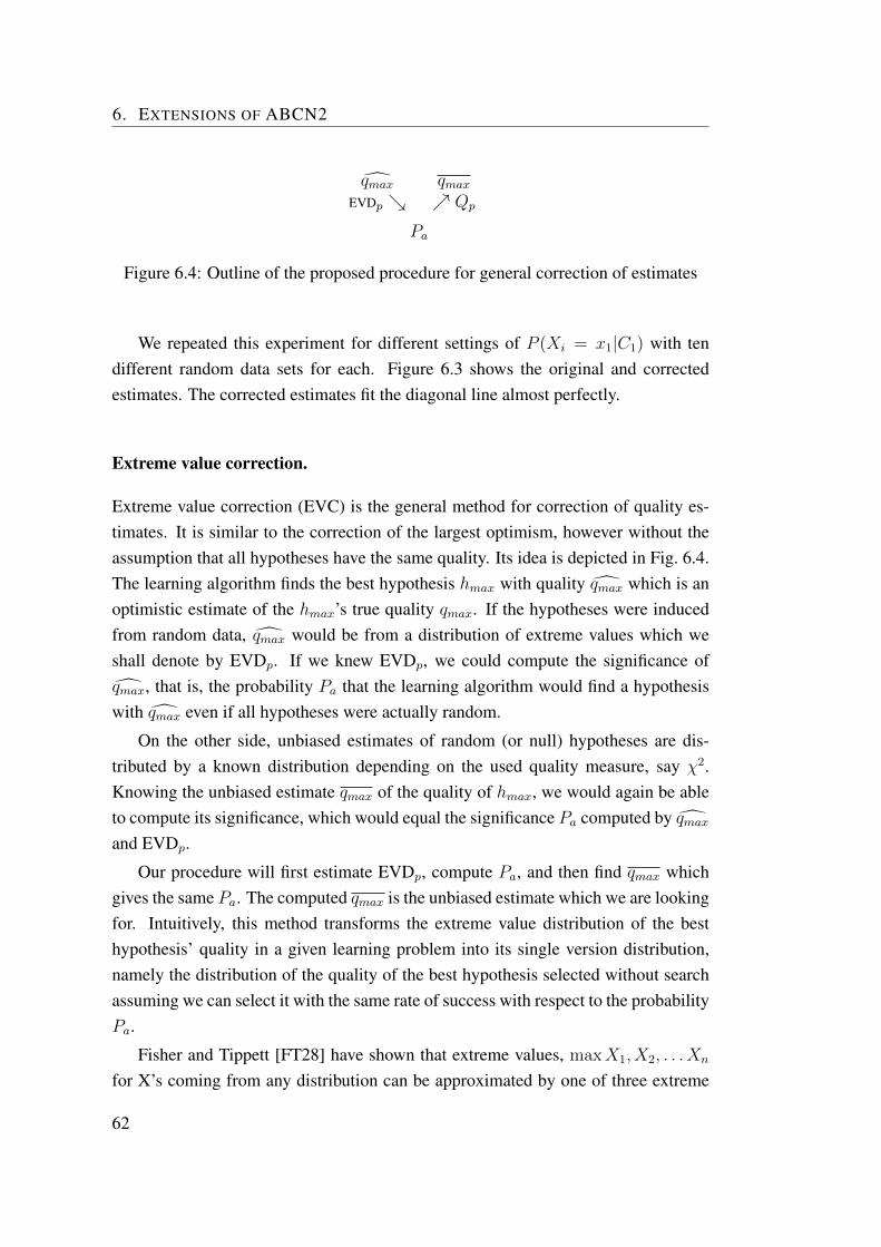
6. EXTENSIONS OF ABCN2
qmax qmaxEVDp ↘ ↗ Qp
Pa
Figure 6.4: Outline of the proposed procedure for general correction of estimates
We repeated this experiment for different settings of P (Xi = x1|C1) with tendifferent random data sets for each. Figure 6.3 shows the original and correctedestimates. The corrected estimates fit the diagonal line almost perfectly.
Extreme value correction.
Extreme value correction (EVC) is the general method for correction of quality es-timates. It is similar to the correction of the largest optimism, however without theassumption that all hypotheses have the same quality. Its idea is depicted in Fig. 6.4.The learning algorithm finds the best hypothesis hmax with quality qmax which is anoptimistic estimate of the hmax’s true quality qmax. If the hypotheses were inducedfrom random data, qmax would be from a distribution of extreme values which weshall denote by EVDp. If we knew EVDp, we could compute the significance ofqmax, that is, the probability Pa that the learning algorithm would find a hypothesiswith qmax even if all hypotheses were actually random.
On the other side, unbiased estimates of random (or null) hypotheses are dis-tributed by a known distribution depending on the used quality measure, say χ2.Knowing the unbiased estimate qmax of the quality of hmax, we would again be ableto compute its significance, which would equal the significance Pa computed by qmaxand EVDp.
Our procedure will first estimate EVDp, compute Pa, and then find qmax whichgives the same Pa. The computed qmax is the unbiased estimate which we are lookingfor. Intuitively, this method transforms the extreme value distribution of the besthypothesis’ quality in a given learning problem into its single version distribution,namely the distribution of the quality of the best hypothesis selected without searchassuming we can select it with the same rate of success with respect to the probabilityPa.
Fisher and Tippett [FT28] have shown that extreme values, maxX1, X2, . . . Xn
for X’s coming from any distribution can be approximated by one of three extreme
62
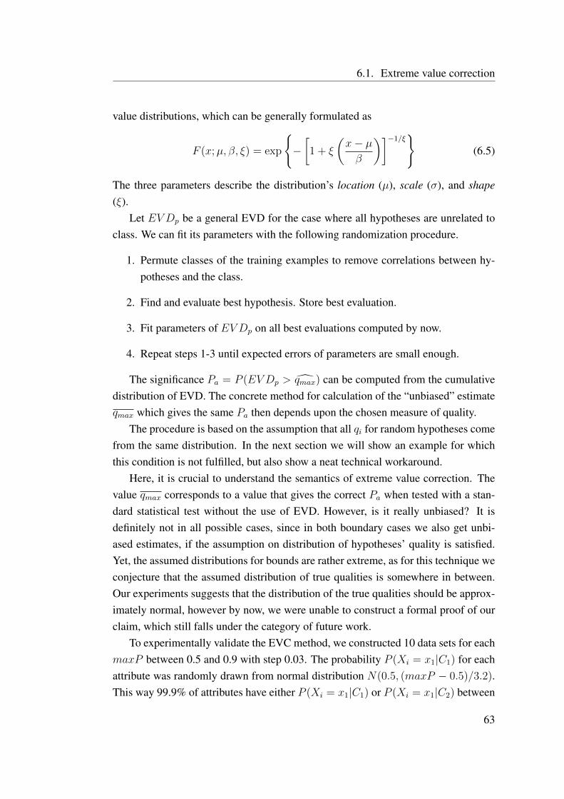
6.1. Extreme value correction
value distributions, which can be generally formulated as
F (x;µ, β, ξ) = exp
{−[1 + ξ
(x− µβ
)]−1/ξ}(6.5)
The three parameters describe the distribution’s location (µ), scale (σ), and shape(ξ).
Let EVDp be a general EVD for the case where all hypotheses are unrelated toclass. We can fit its parameters with the following randomization procedure.
1. Permute classes of the training examples to remove correlations between hy-potheses and the class.
2. Find and evaluate best hypothesis. Store best evaluation.
3. Fit parameters of EVDp on all best evaluations computed by now.
4. Repeat steps 1-3 until expected errors of parameters are small enough.
The significance Pa = P (EVDp > qmax) can be computed from the cumulativedistribution of EVD. The concrete method for calculation of the “unbiased” estimateqmax which gives the same Pa then depends upon the chosen measure of quality.
The procedure is based on the assumption that all qi for random hypotheses comefrom the same distribution. In the next section we will show an example for whichthis condition is not fulfilled, but also show a neat technical workaround.
Here, it is crucial to understand the semantics of extreme value correction. Thevalue qmax corresponds to a value that gives the correct Pa when tested with a stan-dard statistical test without the use of EVD. However, is it really unbiased? It isdefinitely not in all possible cases, since in both boundary cases we also get unbi-ased estimates, if the assumption on distribution of hypotheses’ quality is satisfied.Yet, the assumed distributions for bounds are rather extreme, as for this technique weconjecture that the assumed distribution of true qualities is somewhere in between.Our experiments suggests that the distribution of the true qualities should be approx-imately normal, however by now, we were unable to construct a formal proof of ourclaim, which still falls under the category of future work.
To experimentally validate the EVC method, we constructed 10 data sets for eachmaxP between 0.5 and 0.9 with step 0.03. The probability P (Xi = x1|C1) for eachattribute was randomly drawn from normal distribution N(0.5, (maxP − 0.5)/3.2).This way 99.9% of attributes have either P (Xi = x1|C1) or P (Xi = x1|C2) between
63

6. EXTENSIONS OF ABCN2
0.0 20.0 40.0 60.0
χ2
0.0
20.0
40.0
60.0
80.0
100.0
χ2
..................................................
•••••••••••••••••••
••••••••••••••••••••••••••••••• •••••
•
•••• ••••••••
••
•••••••••• •••••••
••• •••••••••
• •••
•
•
•••••
••••
••
••
•
• •
•
•
•
••••••••••
••••••
.............................................................................
...............................................................
........................................................................................................................................................................................
.....................
(a) Uncorrected χ2
0.0 20.0 40.0 60.0
χ2
0.0
20.0
40.0
60.0
80.0
100.0
χ2
..................................................
•••••••••••••••••••••••••••••••••••••••••••••••••• •••••
•
•••• ••
••••••
••
•••••••••• ••••
•••
••• •••••
••••
• ••
•
•
•
•••••
•
•••
•
•••
•
• •
•
••
••
•••• ••••
•
•
••
•
•
................................................................................
...............................................
............................................................................................................................................................................................................
....................
(b) EVCorrected χ2
Figure 6.5: Original and corrected estimates of χ2. True qualities are distributednormally.
0.5 and maxP . The results of the extreme value correction are shown in Figure 6.5.Again we observe that the original estimates are optimistic while the adjusted valuesmatch the true values very well.
6.2 Extreme value correction in rule learning
Most rule learning algorithms, as well as CN2, induce models by iteratively searchingfor the best rule and removing the examples covered by it [FF05]. Rules are usuallysought by a beam search, which gradually adds conditions to the rule with aim todecrease the number of covered “negative” examples, while at the same time losingas few “positive” examples as possible. The search is guided by two measures, onewhich evaluates the partial rules and the other which selects between the final rulecandidates; here we will use the common approach where the same measure is usedfor both purposes.
A good rule should give accurate class predictions, or, in other words, have a highprobability of the positive class among all examples (not only learning examples)covered by the rule. Hence a reasonable choice for the measure of rule’s quality isthe relative frequency of the predicted class:
qi =sini
(6.6)
64
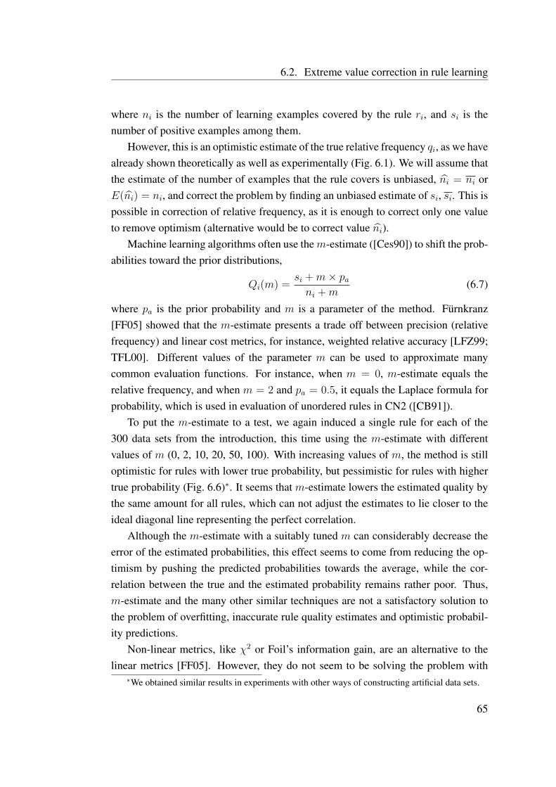
6.2. Extreme value correction in rule learning
where ni is the number of learning examples covered by the rule ri, and si is thenumber of positive examples among them.
However, this is an optimistic estimate of the true relative frequency qi, as we havealready shown theoretically as well as experimentally (Fig. 6.1). We will assume thatthe estimate of the number of examples that the rule covers is unbiased, ni = ni orE(ni) = ni, and correct the problem by finding an unbiased estimate of si, si. This ispossible in correction of relative frequency, as it is enough to correct only one valueto remove optimism (alternative would be to correct value ni).
Machine learning algorithms often use them-estimate ([Ces90]) to shift the prob-abilities toward the prior distributions,
Qi(m) =si +m× pani +m
(6.7)
where pa is the prior probability and m is a parameter of the method. Furnkranz[FF05] showed that the m-estimate presents a trade off between precision (relativefrequency) and linear cost metrics, for instance, weighted relative accuracy [LFZ99;TFL00]. Different values of the parameter m can be used to approximate manycommon evaluation functions. For instance, when m = 0, m-estimate equals therelative frequency, and when m = 2 and pa = 0.5, it equals the Laplace formula forprobability, which is used in evaluation of unordered rules in CN2 ([CB91]).
To put the m-estimate to a test, we again induced a single rule for each of the300 data sets from the introduction, this time using the m-estimate with differentvalues of m (0, 2, 10, 20, 50, 100). With increasing values of m, the method is stilloptimistic for rules with lower true probability, but pessimistic for rules with highertrue probability (Fig. 6.6)∗. It seems that m-estimate lowers the estimated quality bythe same amount for all rules, which can not adjust the estimates to lie closer to theideal diagonal line representing the perfect correlation.
Although the m-estimate with a suitably tuned m can considerably decrease theerror of the estimated probabilities, this effect seems to come from reducing the op-timism by pushing the predicted probabilities towards the average, while the cor-relation between the true and the estimated probability remains rather poor. Thus,m-estimate and the many other similar techniques are not a satisfactory solution tothe problem of overfitting, inaccurate rule quality estimates and optimistic probabil-ity predictions.
Non-linear metrics, like χ2 or Foil’s information gain, are an alternative to thelinear metrics [FF05]. However, they do not seem to be solving the problem with
∗We obtained similar results in experiments with other ways of constructing artificial data sets.
65
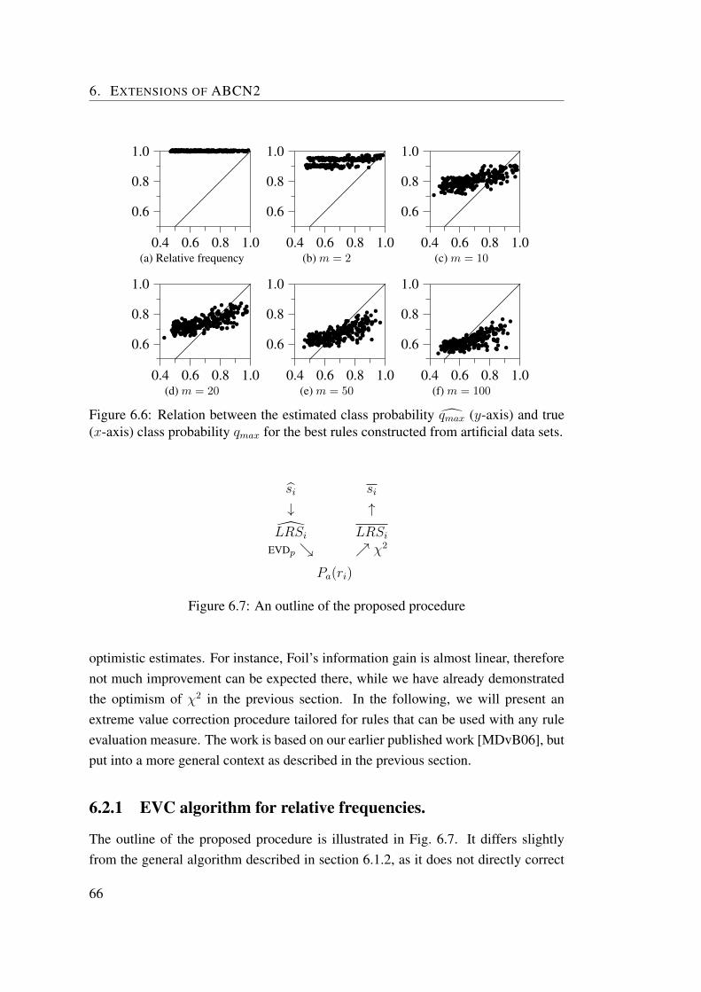
6. EXTENSIONS OF ABCN2
0.4 0.6 0.8 1.0
0.6
0.8
1.0
...................................................................................................................................................................................................................................•••• •• ••• ••• •• •• •• •• •• ••• •• • • •••• • • •• ••• • ••• •• ••• • •••• ••• ••• •• •• • ••• • ••• •• ••• •• • ••• ••• •• • •• •• ••••• •• ••••• • •• • •• •••• •• •• •• ••••• • •• •• •• •••• ••• •• •••• • •••••• •• •• •• ••• •• •• ••• •• ••• ••• •• •• • •• •••••• •• ••• •• ••• •••• •• •••• •• • ••• • •• •• ••• •• •• • ••• ••• •• • •• •• ••• • •• ••••• •• •• • •• •• •• • ••• •• •• ••
(a) Relative frequency0.4 0.6 0.8 1.0
0.6
0.8
1.0
...................................................................................................................................................................................................................................
•••••• ••• ••• •
• ••
•• •••
••
•••• • •
•••• •
• •• ••• • •••
••
••• • •••• ••• ••
••• •• • •
•• •••
••• ••• ••
•••• ••• ••
• •• •• ••••• •• • •
•••• •• • •• •••
• •••
• •••
•••• • ••
•• •• ••••
••••• •
••• • •••••• •• •••• •••••
•• ••• ••••
• ••
• •• •• ••••••••
•••
••••• •
•• •••••
•••••
••• ••• • ••
•• •••••
••
• ••• •
•• •
• ••
••
•••
•••
•••••• •• ••• •• •• ••• ••
• •••• •
•
(b) m = 2
0.4 0.6 0.8 1.0
0.6
0.8
1.0
...................................................................................................................................................................................................................................
••••
••••••
••
•• •••
•••
••
•••
•• •••
•••
•
•••••• •• •••
•
••
••
•••• ••••••
••
••
••
•• •
••
•
•• ••• ••
•
•••••• ••
••• •• •••••
•••
••••• ••
• •• •••• •• •
•••
•••••
••
••
••••
••••
••••
•
• ••• •••••
••• •
•• •••• ••
•• •
••••
••• ••• •• •••••
•••
••• • •••
•
•••
•• ••••
•
••
••
••••
••
• ••
•
•• •• •••
•
•• •
• •••
••• • •••
•
•••
••••• • •• •• ••• •
•
•••
•• ••• •
•
•• •
•
(c) m = 10
0.4 0.6 0.8 1.0
0.6
0.8
1.0
...................................................................................................................................................................................................................................
••••
••••••
•••• ••
•
••
••• ••••• •••
••
••
••• •• • •• •
•
•
•
••
••
•••• •••
•
••
••
••
••
•• •
••
•
•• ••• ••
•
•••••• ••
• •• ••
•••••
••
•••••
• ••• •
• • ••• ••
•• ••
•••••
••
•
•••••
•••
••
•••
•
• ••• •••••
••••
••••
•• ••
•
••
•• ••••
• ••• •• •••••
••
•••• ••
•••
•••
•• ••••
•
•
•••••••
••• ••
•
•• •• • ••
•
•• •
•••• ••
• • •••
•
••
••
•• •• ••• ••
•• • ••
••
••
• •••
•
•
•
••
•
(d) m = 20
0.4 0.6 0.8 1.0
0.6
0.8
1.0
...................................................................................................................................................................................................................................
••••
••••••
•••• ••
•
••
•••
•••
•• ••
•
•••
•••• ••• •••
•
•
•
••
••
•••• ••••
•••
•
••
••
•• •
••
•
•• ••• ••
•••
••••••• •
• ••••
•••
••
•••••
•••
• •• • ••• •••
• ••
•••••
••
••
••••
•••••
••
•
•
• ••
•• •••••••
•
••• ••• • •
•
••
•• ••••
• ••• •• •• •• •
••
•••• ••
•••
•
••
•• ••• •
•
•
•
•••••••
•• ••
•
•••• ••
•
•
•• •
•• •••
••
• ••
•
•••
•••• •• ••• ••
•• ••••
• ••••••
••
•
••
•
(e) m = 50
0.4 0.6 0.8 1.0
0.6
0.8
1.0
...................................................................................................................................................................................................................................
••••
••••••
•• •• ••
•
••
•••
•• •
•• ••
•••
••
••• •• • •••••
•
•••
•••
•• ••••
•••
•
•••
••• •••
•
•• ••• ••
•••
••••••
•••••
•••
••
••
•
•••••••• •
• • ••••• •
• ••
•
• •••
• •
•
•• ••
••••• •••
••
• ••
••••••• •••
••• •••• •
•
•••• ••
• •• ••• •••• •• •
••
•••• ••
•••
•
••
•• •••••
•
•
••••••
••• ••
•
•• •
•••
•
•
•• •
•• ••• •
•• ••
•
•••
•••• ••••••• ••• •••
• ••
•••• •
•
•
••
•
(f) m = 100
Figure 6.6: Relation between the estimated class probability qmax (y-axis) and true(x-axis) class probability qmax for the best rules constructed from artificial data sets.
si si
↓ ↑LRSi LRSi
EVDp ↘ ↗ χ2
Pa(ri)
Figure 6.7: An outline of the proposed procedure
optimistic estimates. For instance, Foil’s information gain is almost linear, thereforenot much improvement can be expected there, while we have already demonstratedthe optimism of χ2 in the previous section. In the following, we will present anextreme value correction procedure tailored for rules that can be used with any ruleevaluation measure. The work is based on our earlier published work [MDvB06], butput into a more general context as described in the previous section.
6.2.1 EVC algorithm for relative frequencies.
The outline of the proposed procedure is illustrated in Fig. 6.7. It differs slightlyfrom the general algorithm described in section 6.1.2, as it does not directly correct
66
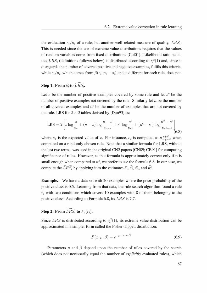
6.2. Extreme value correction in rule learning
the evaluation si/ni of a rule, but another well related measure of quality, LRSi.This is needed since the use of extreme value distributions requires that the valuesof random variables come from fixed distributions [Col01]. Likelihood ratio statis-tics LRSi (definitions follows below) is distributed according to χ2(1) and, since itdisregards the number of covered positive and negative examples, fulfils this criteria,while si/ni, which comes from β(si, ni − si) and is different for each rule, does not.
Step 1: From si to LRSi.
Let s be the number of positive examples covered by some rule and let sc be thenumber of positive examples not covered by the rule. Similarly let n be the numberof all covered examples and nc be the number of examples that are not covered bythe rule. LRS for 2× 2 tables derived by [Dun93] as:
LRS = 2
[s log
s
es+ (n− s) log n− s
en−s+ sc log
sc
esc+ (nc − sc) log n
c − scenc−sc
](6.8)
where ex is the expected value of x. For instance, es is computed as n s+sc
n+nc, when
computed on a randomly chosen rule. Note that a similar formula for LRS, withoutthe last two terms, was used in the original CN2 papers [CN89; CB91] for computingsignificance of rules. However, as that formula is approximately correct only if n issmall enough when compared to nc, we prefer to use the formula 6.8. In our case, wecompute the LRSi by applying it to the estimates si, sci , ni, and nci .
Example. We have a data set with 20 examples where the prior probability of thepositive class is 0.5. Learning from that data, the rule search algorithm found a ruleri with two conditions which covers 10 examples with 8 of them belonging to thepositive class. According to Formula 6.8, its LRS is 7.7.
Step 2: From LRSi to Pa(ri).
Since LRS is distributed according to χ2(1), its extreme value distribution can beapproximated in a simpler form called the Fisher-Tippett distribution:
F (x;µ, β) = e−e−(x−µ)/β
(6.9)
Parameters µ and β depend upon the number of rules covered by the search(which does not necessarily equal the number of explicitly evaluated rules), which
67
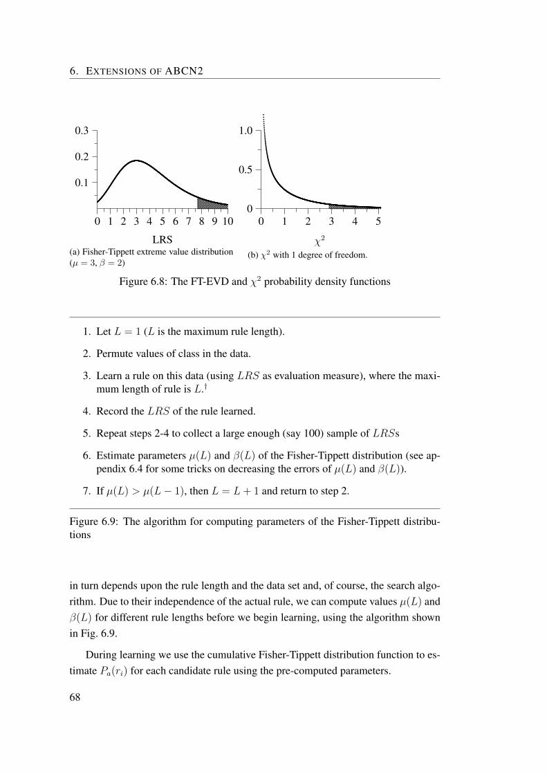
6. EXTENSIONS OF ABCN2
0 1 2 3 4 5 6 7 8 9 10
LRS
0.1
0.2
0.3
.......................................................................................................................................................................................................................................................................
..............................................................................................................................................................................................................................................................................................................................................................................................................................................................................................................................................................................................................................................................................................................................................................................................
....
..................................................................................................................................
(a) Fisher-Tippett extreme value distribution(µ = 3, β = 2)
0 1 2 3 4 5
χ2
0
0.5
1.0
........................................................................................................................................................................................................................................................................................................................................................................................................................................................................................................................................................................................................................................................................................................................................................................................................................................................................................................................................................................................................................................................................................................................................
(b) χ2 with 1 degree of freedom.
Figure 6.8: The FT-EVD and χ2 probability density functions
1. Let L = 1 (L is the maximum rule length).
2. Permute values of class in the data.
3. Learn a rule on this data (using LRS as evaluation measure), where the maxi-mum length of rule is L.†
4. Record the LRS of the rule learned.
5. Repeat steps 2-4 to collect a large enough (say 100) sample of LRSs
6. Estimate parameters µ(L) and β(L) of the Fisher-Tippett distribution (see ap-pendix 6.4 for some tricks on decreasing the errors of µ(L) and β(L)).
7. If µ(L) > µ(L− 1), then L = L+ 1 and return to step 2.
Figure 6.9: The algorithm for computing parameters of the Fisher-Tippett distribu-tions
in turn depends upon the rule length and the data set and, of course, the search algo-rithm. Due to their independence of the actual rule, we can compute values µ(L) andβ(L) for different rule lengths before we begin learning, using the algorithm shownin Fig. 6.9.
During learning we use the cumulative Fisher-Tippett distribution function to es-timate Pa(ri) for each candidate rule using the pre-computed parameters.
68

6.2. Extreme value correction in rule learning
Example (continued). Say that the algorithm from Fig. 6.9 found µ(2) = 3 andβ(2) = 2 (remember that rule r has two conditions). The curve with such parame-ters is depicted in Fig. 6.8, so the probability Pa(ri) for the rule from our examplecorresponds to the shaded area right of LRS=7.7. Pa(r) equals approximately 0.09.
Step 3: From Pa(ri) to LRSi.
To compute LRSi we need to do the opposite from the last step. Looking at the χ2(1)
distribution (Fig. 6.8), we need to find such a value of LRSi that the area under thecurve to the right of it will equal the computed Pa(ri). In other words, the shadedareas under the curves in Fig. 6.8 should be the same.
Example (continued). The corresponding LRSi for our examples as read from Fig.6.8 is 2.9. Note that this is much less than LRS = 7.7, which we computed directlyfrom the data and which would essentially be used by an unmodified rule inductionalgorithm.
Step 4: From LRSi to si.
The remaining task is trivial: compute si from the formula for LRSi using an arbi-trary root finding algorithm. In our task we are correcting probability estimates basedon relative frequencies, so we shall compute them by dividing the corrected si by ni.
Example (conclusion). We used Brent’s method [Atk89] to find that LRSi = 2.9
corresponds to si = 6.95. The rule covers ten examples, so the corresponding classprobability is 6.95/10 = 0.695. Note that this estimate is quite smaller than theuncorrected 0.8.
6.2.2 Extreme value corrected relative frequency in PN space
PN-space, introduced by Furnkranz [FF05], is a visualization of rule evaluation met-rics and their behavior at different coverages and ratios between positive and negativeexamples. The isometrics in a such diagram connect different combinations of cov-ered positive and negative examples that are given the same quality by the selectedmeasure.
†Note that usingLRS at a given rule length will always order rules the same as wouldLRS. How-ever, as we will be using si/ni in the actual learning phase, in order to correctly estimate parametersof Fisher-Tippett distribution, measures s/n and LRSi should be well correlated.
69
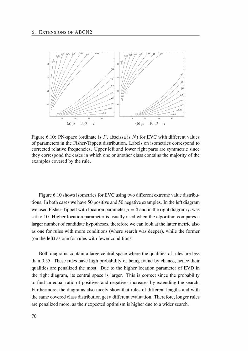
6. EXTENSIONS OF ABCN2
0.55
0.55
0.6
0.6
0.65
0.65
0.7
0.7
0.75
0.75
0.8
0.8
0.85
0.85
0.9
0.9
10 20 30 40
10
20
30
40
(a) µ = 3, β = 2
0.55
0.550.6
0.6
0.65
0.65
0.7
0.7
0.75
0.75
0.8
0.8
0.85
0.85
0.9
0.9
10 20 30 40
10
20
30
40
(b) µ = 10, β = 2
Figure 6.10: PN-space (ordinate is P , abscissa is N ) for EVC with different valuesof parameters in the Fisher-Tippett distribution. Labels on isometrics correspond tocorrected relative frequencies. Upper left and lower right parts are symmetric sincethey correspond the cases in which one or another class contains the majority of theexamples covered by the rule.
Figure 6.10 shows isometrics for EVC using two different extreme value distribu-tions. In both cases we have 50 positive and 50 negative examples. In the left diagramwe used Fisher-Tippett with location parameter µ = 3 and in the right diagram µ wasset to 10. Higher location parameter is usually used when the algorithm compares alarger number of candidate hypotheses, therefore we can look at the latter metric alsoas one for rules with more conditions (where search was deeper), while the former(on the left) as one for rules with fewer conditions.
Both diagrams contain a large central space where the qualities of rules are lessthan 0.55. These rules have high probability of being found by chance, hence theirqualities are penalized the most. Due to the higher location parameter of EVD inthe right diagram, its central space is larger. This is correct since the probabilityto find an equal ratio of positives and negatives increases by extending the search.Furthermore, the diagrams also nicely show that rules of different lengths and withthe same covered class distribution get a different evaluation. Therefore, longer rulesare penalized more, as their expected optimism is higher due to a wider search.
70
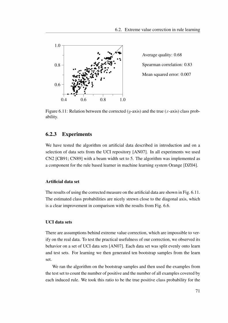
6.2. Extreme value correction in rule learning
0.4 0.6 0.8 1.0
0.6
0.8
1.0
.....................................................................................................................................................................................................................................................................................................................................................................................................................................................................
•
••
•
•
•
•
••
•
•
•
•
•
•
•
•
•
•
•
•
•
•
• •
•
•
•
•
•
•
•
•
•
••
••
••
•••
•
•
•
•
•
•
•
•
••
•
•
•
•
•
•
•
•
•
•
•
••
•
••
••
•
•
•
•
•
•
•
•
•
•
•
•
••
•••
••
• •
•
••
••
•
••
•
•
•
••
•
•
•
•
•
•
•
•
•
•
•••
• •
•
•
•
••
•
•
•
•
•
•
••
•
•
•
•
•
•
•
•
•
•
• •
•
•
•
••••
•
•
•
•
•
••
•
•
• •
•
•
•
•
•
••
•
•
•
•
•
•
• •
••
•
•
••
•
•
•
• ••
••
••
•
••
•
••
••
•
•
•
•
•
•
••
•
•
•
•
•
•
•
•
•
•• •
•
••
•
•
•
•
•
••
•
••
•
•
••
•
•
•
•
•
•
•
••
•
• ••
• •
•
•
•
••
•
•
•
•
•
••
••
•
•
•
•
•
•
Average quality: 0.68
Spearman correlation: 0.83
Mean squared error: 0.007
Figure 6.11: Relation between the corrected (y-axis) and the true (x-axis) class prob-ability.
6.2.3 Experiments
We have tested the algorithm on artificial data described in introduction and on aselection of data sets from the UCI repository [AN07]. In all experiments we usedCN2 [CB91; CN89] with a beam width set to 5. The algorithm was implemented asa component for the rule based learner in machine learning system Orange [DZ04].
Artificial data set
The results of using the corrected measure on the artificial data are shown in Fig. 6.11.The estimated class probabilities are nicely strewn close to the diagonal axis, whichis a clear improvement in comparison with the results from Fig. 6.6.
UCI data sets
There are assumptions behind extreme value correction, which are impossible to ver-ify on the real data. To test the practical usefulness of our correction, we observed itsbehavior on a set of UCI data sets [AN07]. Each data set was split evenly onto learnand test sets. For learning we then generated ten bootstrap samples from the learnset.
We ran the algorithm on the bootstrap samples and then used the examples fromthe test set to count the number of positive and the number of all examples covered byeach induced rule. We took this ratio to be the true positive class probability for the
71
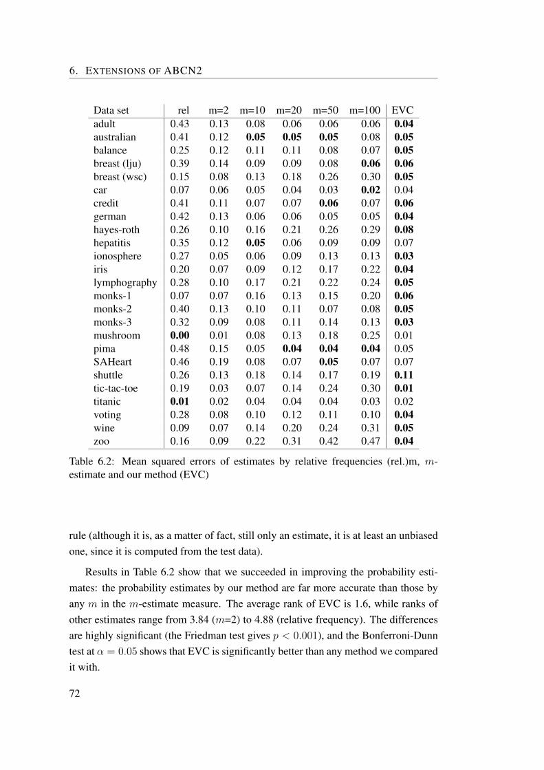
6. EXTENSIONS OF ABCN2
Data set rel m=2 m=10 m=20 m=50 m=100 EVCadult 0.43 0.13 0.08 0.06 0.06 0.06 0.04australian 0.41 0.12 0.05 0.05 0.05 0.08 0.05balance 0.25 0.12 0.11 0.11 0.08 0.07 0.05breast (lju) 0.39 0.14 0.09 0.09 0.08 0.06 0.06breast (wsc) 0.15 0.08 0.13 0.18 0.26 0.30 0.05car 0.07 0.06 0.05 0.04 0.03 0.02 0.04credit 0.41 0.11 0.07 0.07 0.06 0.07 0.06german 0.42 0.13 0.06 0.06 0.05 0.05 0.04hayes-roth 0.26 0.10 0.16 0.21 0.26 0.29 0.08hepatitis 0.35 0.12 0.05 0.06 0.09 0.09 0.07ionosphere 0.27 0.05 0.06 0.09 0.13 0.13 0.03iris 0.20 0.07 0.09 0.12 0.17 0.22 0.04lymphography 0.28 0.10 0.17 0.21 0.22 0.24 0.05monks-1 0.07 0.07 0.16 0.13 0.15 0.20 0.06monks-2 0.40 0.13 0.10 0.11 0.07 0.08 0.05monks-3 0.32 0.09 0.08 0.11 0.14 0.13 0.03mushroom 0.00 0.01 0.08 0.13 0.18 0.25 0.01pima 0.48 0.15 0.05 0.04 0.04 0.04 0.05SAHeart 0.46 0.19 0.08 0.07 0.05 0.07 0.07shuttle 0.26 0.13 0.18 0.14 0.17 0.19 0.11tic-tac-toe 0.19 0.03 0.07 0.14 0.24 0.30 0.01titanic 0.01 0.02 0.04 0.04 0.04 0.03 0.02voting 0.28 0.08 0.10 0.12 0.11 0.10 0.04wine 0.09 0.07 0.14 0.20 0.24 0.31 0.05zoo 0.16 0.09 0.22 0.31 0.42 0.47 0.04
Table 6.2: Mean squared errors of estimates by relative frequencies (rel.)m, m-estimate and our method (EVC)
rule (although it is, as a matter of fact, still only an estimate, it is at least an unbiasedone, since it is computed from the test data).
Results in Table 6.2 show that we succeeded in improving the probability esti-mates: the probability estimates by our method are far more accurate than those byany m in the m-estimate measure. The average rank of EVC is 1.6, while ranks ofother estimates range from 3.84 (m=2) to 4.88 (relative frequency). The differencesare highly significant (the Friedman test gives p < 0.001), and the Bonferroni-Dunntest at α = 0.05 shows that EVC is significantly better than any method we comparedit with.
72

6.2. Extreme value correction in rule learning
This would, however, be easily achieved and surpassed by a method returning asingle rule covering all examples and which would estimate the probability with theprior class probability. To test that our gains are not due to oversimplification wealso computed the average AUC over the ten bootstrap samples. To make predictionsfrom lists of rules, we used a simple classifier that takes the first rule that triggers foreach class (we get one rule for each class), and normalize the class probabilities ofthese rules to sum up to 1. Although there exist better classifiers from a set of rules,we believe that using them would not considerably change the ranking of examplesand the related AUC. Table 6.3 shows that the performance of our method in termsof AUC is comparable to that of the other methods. The differences here are lesssignificant (the Friedman test gives p = 0.64), and the Bonferroni-Dunn test does notrecognize the EVC as being significantly better than the other methods.
6.2.4 Extreme value correction in argument based rule learning
In the induction of an argument-based rule, the algorithm searches a smaller rulespace when compared to learning standard rules. The larger impact on search reduc-tion is due to the reasons of positive arguments that comprise the condition part ofthe rule. The part of the rule stemming from an argument is not a result of search, butprovided from expert, and therefore is not the culprit for optimism in rules. The EVCshould thus correct only the optimism “produced” by the other part of the condition.The negative arguments, on the other hand, have only a negligible effect in reducingthe size of the search space and do not need to be considered by EVC.
The only required change to the original EVC algorithm is to learn the param-eters µ and β for all possible initial size of arguments. The Algorithm is shown inFigure 6.12. The result is a set of parameters µ and β for each possible length of arule and each possible length of the argument in the rule. When a rule in ABCN2 isevaluated, use the corresponding parameters given rule length L and argument lengthA.
6.2.5 When extreme value correction should be used?
The EVC method commits to the following three main assumptions:
• Number of candidate hypotheses should be high enough. Otherwise the maxi-mum values will not converge to the extreme value distribution, and the related
73

6. EXTENSIONS OF ABCN2
Data set rel m=2 m=10 m=20 m=50 m=100 EVCadult 0.74 0.76 0.76 0.77 0.77 0.78 0.84australian 0.85 0.87 0.88 0.88 0.88 0.88 0.91balance 0.82 0.81 0.81 0.82 0.82 0.81 0.82breast (lju) 0.60 0.62 0.60 0.58 0.60 0.60 0.62breast (wsc) 0.97 0.97 0.97 0.97 0.96 0.96 0.98car 0.84 0.84 0.85 0.86 0.89 0.90 0.90credit 0.82 0.88 0.88 0.88 0.87 0.88 0.91german 0.69 0.68 0.69 0.68 0.69 0.69 0.73hayes-roth 0.88 0.89 0.87 0.86 0.87 0.86 0.90hepatitis 0.77 0.76 0.76 0.73 0.73 0.71 0.77ionosphere 0.90 0.91 0.89 0.89 0.89 0.91 0.92iris 0.97 0.95 0.95 0.95 0.95 0.95 0.95lymphography 0.78 0.81 0.83 0.85 0.84 0.83 0.81monks-1 1.00 1.00 1.00 1.00 1.00 1.00 1.00monks-2 0.66 0.67 0.66 0.66 0.64 0.65 0.64monks-3 0.97 0.98 0.99 0.99 0.99 0.99 0.99mushroom 1.00 1.00 1.00 1.00 1.00 1.00 1.00pima 0.68 0.72 0.72 0.72 0.72 0.73 0.76SAHeart 0.59 0.62 0.63 0.63 0.65 0.65 0.65shuttle 0.99 0.98 0.98 0.99 0.99 0.99 0.98tic-tac-toe 0.96 1.00 1.00 1.00 0.99 0.94 1.00titanic 0.77 0.77 0.77 0.77 0.77 0.77 0.77voting 0.95 0.95 0.96 0.96 0.97 0.97 0.96wine 0.97 0.98 0.98 0.98 0.98 0.98 0.94zoo 1.00 0.99 0.99 0.99 0.99 0.99 0.99
Table 6.3: AUC of classification rules constructed using relative frequencies (rel.)m,m-estimate and our method (EVC)
probability Pa could not be correctly estimated. Number of hypotheses is pos-itively related to the number of attributes, independence between attributes,number of examples, and complexity of hypotheses space.
• Distributions of hypotheses’ qualities should be approximately normal. Espe-cially problematic are cases with only a few good hypotheses, while others aremuch worse. In such a case, EVC will still find the best hypothesis, but EVCwill penalise it more than needed.
• The true evaluation of the best hypothesis is close to 1.0. The problem of ex-treme situations, where the best evaluation is close to the maximum possible
74
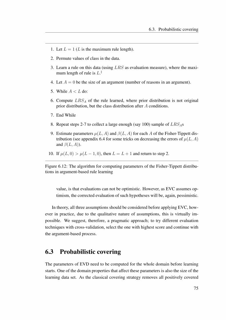
6.3. Probabilistic covering
1. Let L = 1 (L is the maximum rule length).
2. Permute values of class in the data.
3. Learn a rule on this data (using LRS as evaluation measure), where the maxi-mum length of rule is L.‡
4. Let A = 0 be the size of an argument (number of reasons in an argument).
5. While A < L do:
6. Compute LRSA of the rule learned, where prior distribution is not originalprior distribution, but the class distribution after A conditions.
7. End While
8. Repeat steps 2-7 to collect a large enough (say 100) sample of LRSAs
9. Estimate parameters µ(L,A) and β(L,A) for each A of the Fisher-Tippett dis-tribution (see appendix 6.4 for some tricks on decreasing the errors of µ(L,A)and β(L,A)).
10. If µ(L, 0) > µ(L− 1, 0), then L = L+ 1 and return to step 2.
Figure 6.12: The algorithm for computing parameters of the Fisher-Tippett distribu-tions in argument-based rule learning
value, is that evaluations can not be optimistic. However, as EVC assumes op-timism, the corrected evaluation of such hypotheses will be, again, pessimistic.
In theory, all three assumptions should be considered before applying EVC, how-ever in practice, due to the qualitative nature of assumptions, this is virtually im-possible. We suggest, therefore, a pragmatic approach; to try different evaluationtechniques with cross-validation, select the one with highest score and continue withthe argument-based process.
6.3 Probabilistic covering
The parameters of EVD need to be computed for the whole domain before learningstarts. One of the domain properties that affect these parameters is also the size of thelearning data set. As the classical covering strategy removes all positively covered
75

6. EXTENSIONS OF ABCN2
example ([CB91]), we would need to re-estimate these parameters each time whena rule is induced and the covered examples are removed. The alternative could beweighted covering algorithm proposed by [LFTW04], where each example’s weightin learning is inversely related to the number of rules covering it. However, suchstrategy changes the class distribution after each learned rule, which also affects theparameters of EVD. Unfortunately, estimation of the parameters is time consuming,and re-estimating parameters each time a rule is learned would make the use of EVCwith the standard CN2 covering procedure or with weighted covering algorithm veryinefficient. To evade the problem we propose a new strategy called probabilisticcovering strategy where the number of learning examples and their class distributionremains constant during the complete induction process.
Let x.prob be the quality of the best rule covering x. If there are no rules coveringx then x.prob equals the prior probability of the example’s class. When a new ruleR is learned, the removing procedure updates all probabilities of covered examplesas x.prob = maximum(x.prob, q(R)), where q(R) is as usual the estimated classprobability in rule. We say that, when an example x becomes covered by a newrule, where q(R) > x.prob, then rule R improves the probability of this example; orshorter: rule R improves example x. We call this probabilistic covering.
Furthermore, we have to enforce certain changes to the procedure of learning asingle rule to prevent learning the same rule all over again, as probabilistic coveringonly records how well an example is explained and does not affect the way in whicha rule is learned. We propose the following changes:
Selection of best rule A new rule can be learned only if it improves at least oneexample. This must be added as a condition in the algorithm.
Selection of N most promising rules (star) In the original CN2 algorithm best Nrules are selected according to q(R). This heuristic fails in our case, as we seekfor a rule that has high quality and will improve at least one example. Let Zbe a variable with normal distribution approximating the binomial distributionof a rule R. Its parameters are:
µ = |XR| × r(Q)σ2 = |XR| × r(Q)(1− r(Q))
The probability 1−P (Z < x.prob) is the probability that a randomly selectedvalue with given average and variance will be higher than x.prob, which we
76
6.4. Computing parameters of extreme-value distribution
take as a measure of hardness to improve the example x with a specialisationof rule R. Furthermore, if the probability is interpreted as the probability ofimproving example x, then the formula
EI(R) =∑xi∈XR
[1.0− P (Z < x.prob)] (6.10)
corresponds to the expected number of improved examples from a rule. Thisis the formula used in ABCN2 to select the N most promising rules.
Probabilistic rule covering is evaluated in the next chapter together with the PI-LAR classification technique.
6.4 Computing parameters of extreme-valuedistribution
Section 6.2.1 describes an algorithm for computing extreme distributions of ruleslearned from random data which involves calculating the parameters of extremevalue distribution for a vector of maxima of evaluations of rules distributed by χ2
with 1 degree of freedom. The limiting distribution of all χ2 distributions is Fisher-Tippet ([FT28; Gum54; GL54]).
The cumulative distribution function of Fisher-Tippet distribution is
P (x < x0) = e−eµ−x0β (6.11)
where µ and β are parameters of the distribution. Distribution’s mean, median, andvariance are
mean = µ+ βγ, median = µ− β ∗ ln ln 2, var = π2β2/6 (6.12)
where γ is Euler-Mascheroni constant 0.57721. The natural way to compute theparameters µ and β from the sample would be to first estimate the variance fromthe data and use it to compute β, followed by the estimation of µ from the sample’smean or median. However, the error of estimation of variance and mean propagatesto estimations of parameters µ and β, where variance is a bigger problem than mean,as it is used for estimation of both parameters.
Gupta [Gup60] showed that for p independent and identically distributed valuestaken from χ2 with one degree of freedom, where p is large, the following properties
77

6. EXTENSIONS OF ABCN2
hold for their maxima M :
E(M) = 2 ln p− ln ln p− ln π + 2γ (6.13)
m(M) = 2 ln p− ln ln p− ln π − 2 ln ln 2 (6.14)
σ(M) =√
2/3π2 (6.15)
Since σ(M) is independent of the number of values p (although it has to be large),combining 6.12 and 6.15 gives β = 2. On the other hand, when p is not large, βwill be less than 2, as the variance of χ2 is less than the variance of its correspond-ing extreme value distribution. Particularly, in the extreme case with p = 1, theFisher-Tippet would try to approximate the χ2 distribution, where β would be 1.1.Therefore, to compute β, we need to first estimate the variance of extreme values,compute β, and trim it to values between 1.1 an 2.
Afterwards β was estimated, we can proceed to estimation of the remaining pa-rameter µ. In our algorithm we computed the median from the vector of maximumvalues, so µ equals the median plus β ln ln 2.
78
Chapter 7
Classification from Rules andCombining ABCN2 with OtherMethods
The main advantage of rule learning methods is in their power to spot and explainlocal regularities. Each rule concisely explains the correlation between the class anda set of attributes on the subspace covered by the rule. Their locality, however, raisesproblems when used in classification, as in some cases clashes occur and sometimesthere are no rules that would cover the example to be classified. In the former casewe need to apply any of the available conflict resolution strategies, while in the latterthe default class is the most obvious choice.
In this chapter, we shall first give a short review of different approaches used forclassification from rules and then describe a novel one called PILAR (ProbabilisticImprovement of Learning Algorithms with Rules). PILAR is an algorithm for re-solving rule-conflicts and also for combining rule learning with any other machinelearning method. As shown at the end of the Chapter, it is possible with PILARimplicitly make any machine learning method capable of learning with arguments.
PILAR receives as input a base method and a set of unordered rules. By compar-ing probability predictions of the base method with class probabilities in given rules,the algorithm then observes whether in any of the patterns described with rules, thereis a significant difference in probabilistic prediction of the base method and the cor-responding rule. In such a situation, the prediction of the base method is accordinglycorrected.
The main idea of the algorithm is to represent given rules as constraints. These
79

7. CLASSIFICATION FROM RULES AND COMBINING ABCN2 WITH OTHER
METHODS
constraints are used in an optimisation algorithm that makes the base method con-sistent with these constraints. The algorithm is experimentally evaluated with twobase methods; majority classifier (as classification from rules only) and logistic re-gression (linear probabilistic classifier that can not account for interactions betweenattributes).
7.1 Related work
Lindgren [Lin04] described several approaches to combining conflicting rules. Theycan be divided into simple approaches, e.g. the original CN2 classification and naiveBayesian classification and in more complicated meta-learning techniques that learnon the subset of examples covered by conflicting rules in classification. Lindgrenshowed that the latter techniques do achieve better classification accuracies, howeverthey are inappropriate for our needs - we need the classifications to be explainable inorder to reflect arguments in rules.
Another family of methods for combining conflicting rules falls into the categoryof ensemble methods. Normally, one could think that any kind of ensemble learn-ing is far from interpretable, however in the case of rule learning the learned modelis simply a linear sum of rules’ contributions. Eventually, the induced model is notmuch different from a linear regression model, whereas rules act as variables. Thefirst such system was SLIPPER [CS99] that combined the idea of boosting [FS97]with the RIPPER [Coh95] algorithm. Variations of the ensemble learning princi-ple can be later found in several methods for rule aggregation [WI00; RK06; FP08;DKS08]. We also decided that our algorithm PILAR should induce a linear classifierfrom rules. We will give a detailed motivation for our decision later in the Chapter.
7.2 The PILAR algorithm
The problem described above can be formalized as follows.
Inputs:
• A set of learning examples X = {(x1, y1), . . . , (xn, yn)}, where one exampleis as usual a pair of attribute-values and a class value. Let the domain of classvariable be values c1, . . . , cm.
80

7.2. The PILAR algorithm
• A global classification model M . The expression Mj(xi) returns the probabil-ity of class cj for example xi.
• A set of probabilistic unordered rules R = R1, . . . , Rk. Each rule Ri has acondition part defining the subspace covered by the rule, a class predicted bythe rule, and the probability of predicted class given conditions.
Output:
A corrected classification model M ′, based on M and consistent with the probabilis-tic predictions of rules R.
7.2.1 Log-linear sum of unordered rules
Let x be an example we would like to classify. We define the log-linear model forcorrection of classification model M in two-class domains (c0, c1) as a weighted sum(W is a real-valued vector):
f(x) = lnM1(x)
1−M1(x)+ W · R(x) =
= lnM1(x)
1−M1(x)+ w0 + w1 ×R1(x) + . . .+ wk ×Rk(x), (7.1)
where M1(x) is the probability given by the base method for class c1 and weightsw1, . . . , wk given to rules are all nonnegative reals. The term Ri(x) is defined as:
Ri(x) =
0, if conditions of Ri are false for example x;1, if Ri predicts class c1;−1, if Ri predicts class c0.
(7.2)
The predicted probability of class c1 for example x is computed from f(x) throughthe logit link function:
P (c1|x) =M ′1(x) =
1
1 + e−f(x)(7.3)
Although this particular model can only be used in domains with two classes, itcan be extended to its multi-class version, in the same way as basic logistic regres-sion is extended into a multinomial logistic regression [HL00]. We mentioned thatall the weights should be nonnegative. Negative weights are implausible, since therule’s effect on P (c1|x) would be inconsistent with the rule’s class in conclusion. For
81

7. CLASSIFICATION FROM RULES AND COMBINING ABCN2 WITH OTHER
METHODS
example, a rule predicting class c1 should not be allowed to decrease the probabilityP (c1|x).
The motivation for using log-linear classification from rules comes from its fol-lowing four features:
1. Natural translation from the weighted sum to probabilistic prediction. Regard-less of the value of f(x), the predicted probability P (c1|x) will always bebetween 0 and 1.
2. Handling correlations between rules. If two rules are dependent (or even thesame in the most extreme case), the method for fitting weights can assign alower weight to one of these two rules.
3. Handling conflicting rules. These rules will have differently signed contribu-tions in the log-linear sum, hence the probability predicted to examples whereboth rules trigger will be somewhere in between the probabilities predicted toexamples where only one or the other rule triggers.
4. Log-linear model enables simple and understandable explanations of classifi-cations by the means of a nomogram [Har01; MDKZ04]. The nomograms weresuccessfully used for several methods that can employ a log-linear model (e.g.logistic regression, SVM, etc.). We show a visualisation of a model obtainedfrom rules in Chapter 7.3.4.
7.2.2 Rules as constraints
We will first describe the transformation of a set of rules into a set of constraintsthat should be satisfied by the corrected classification model M ′. Remember that aprobabilistic IF-THEN rule R has the following structure:
IF Complex THEN PR(cj)
The condition term Complex determines the examples that are covered by this rule,while the conclusion predicts class cj and an estimation PR(cj) of its conditionalprobability P (cj|Complex). It will soon be evident that the estimation PR(cj) needsto be unbiased, namely, it gives an estimation of the true conditional probabilityP (cj|Complex), if averaged over all possible subsets drawn from the populationwhere Complex is true. Therefore, we shall use the EVC method to compute PR(cj),which was shown to decrease bias due to extensive searching (see Chapter 6).
82
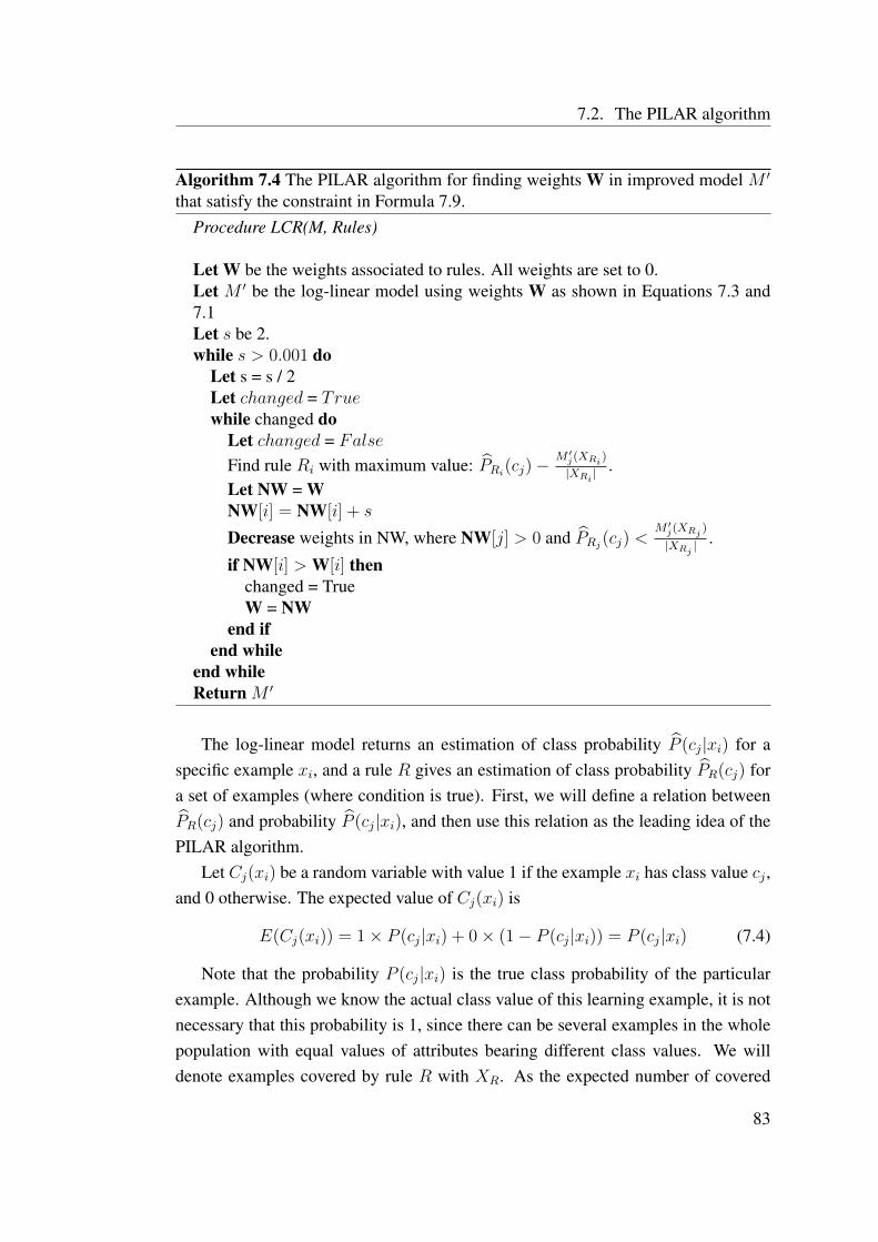
7.2. The PILAR algorithm
Algorithm 7.4 The PILAR algorithm for finding weights W in improved model M ′
that satisfy the constraint in Formula 7.9.Procedure LCR(M, Rules)
Let W be the weights associated to rules. All weights are set to 0.Let M ′ be the log-linear model using weights W as shown in Equations 7.3 and7.1Let s be 2.while s > 0.001 do
Let s = s / 2Let changed = Truewhile changed do
Let changed = FalseFind rule Ri with maximum value: PRi(cj)−
M ′j(XRi )
|XRi |.
Let NW = WNW[i] = NW[i] + s
Decrease weights in NW, where NW[j] > 0 and PRj(cj) <M ′j(XRj )
|XRj |.
if NW[i] > W[i] thenchanged = TrueW = NW
end ifend while
end whileReturn M ′
The log-linear model returns an estimation of class probability P (cj|xi) for aspecific example xi, and a rule R gives an estimation of class probability PR(cj) fora set of examples (where condition is true). First, we will define a relation betweenPR(cj) and probability P (cj|xi), and then use this relation as the leading idea of thePILAR algorithm.
Let Cj(xi) be a random variable with value 1 if the example xi has class value cj ,and 0 otherwise. The expected value of Cj(xi) is
E(Cj(xi)) = 1× P (cj|xi) + 0× (1− P (cj|xi)) = P (cj|xi) (7.4)
Note that the probability P (cj|xi) is the true class probability of the particularexample. Although we know the actual class value of this learning example, it is notnecessary that this probability is 1, since there can be several examples in the wholepopulation with equal values of attributes bearing different class values. We willdenote examples covered by rule R with XR. As the expected number of covered
83

7. CLASSIFICATION FROM RULES AND COMBINING ABCN2 WITH OTHER
METHODS
positive examples (again, it can be different from the actual number) in XR is theexpected sum of all Cj(xi) from XR, and,
E
( ∑xi∈XR
Cj(xi)
)=∑xi∈XR
E(Cj(xi)) =∑xi∈XR
P (cj|xi) (7.5)
the expected number of examples from class cj in examples XR is the sum of allprobabilities for class cj in examples fromXR. LetM ′
j(XR) be the sum of probabilityestimations given by our log-linear model over examples XR:
M ′j(XR) =
∑xi∈XR
P (cj|xi) (7.6)
Then,M ′j(XR) is an estimation of
∑xi∈XR P (cj|xi). The true conditional probability
of class cj of rule R is:
PR(cj) =
∑xi∈XR P (cj|xi)|XR|
(7.7)
TheM ′j(XR)
|XR|is thus an estimation of PR(cj), therefore the following equality could be
used as a constraint on the learned model:
M ′j(XR)
|XR|= PR(cj) (7.8)
We say that a rule is consistent with the prediction of a global model when the aboveconstraint holds. Ideally, we would like to assign such weights to the rules in thelog-linear model that would make all rules consistent. However, in real situations,this is rarely satisfiable. For example, estimation of class probability in a rule some-times depends on rule properties (e.g. rule length), and in such situations we couldencounter two different rules covering the same set of examples XR, while havingdifferent estimations of class probabilities PR(cj). Hence, for the sake of applicabil-ity, we need to relax the “ideal” constraint.
The next constraint is based on the following idea: ifM ′j(XR)
|XR|is higher than PR(cj)
and the rule’s weight is 0, while other rules are consistent with the model, then ruleR is redundant with respect to other rules and is not needed in the model. Therefore,we would like to have a model that uses only a subset of rules in classification, anddisregard redundant ones. This can be formulated as constraint:
∀Ri :
(M ′
j(XRi)
|XRi |= PRi(cj) ∧ wi ≥ 0
)∨(M ′
j(XRi)
|XRi |> PRi(cj) ∧ wi = 0
)(7.9)
where cj is the class predicted by the rule Ri. This constraint is always satisfiable.The algorithm that computes such weights is shown as Algorithm 7.4.
84

7.3. Evaluation
7.3 Evaluation
PILAR is an algorithm for improving a learning method on attribute subspaces in-dicated by classification rules. In the extreme case, where the base method is themajority classifier, PILAR acts as an approach for classification from rules. This willalso be the subject of our initial evaluation, where PILAR will be compared to someother strategies for resolving conflicting rules. Later, we will use PILAR to improvelogistic regression and compare its results with the basic logistic regression, and fi-nally we will show a visualisation of a model produced by PILAR with a nomogram.
7.3.1 Linear models vs. non-linear models
The first experiment serves as a motivation for using linear models. A comparisonbetween PILAR (learns a linear model) and several other techniques will show thatlinear models perform better than the selected non-linear. Currently there are severalnon-linear approaches available for classification from unordered rules. They couldbe classified in two classes; some of them are simple [CB91] and enable classification“by hand”, but they usually perform worse with respect to accuracy than some moresophisticated methods [Lin04]. As already mentioned, the latter methods are notappropriate for our purpose, because they are less understandable, therefore we shallhere compare PILAR only to the former methods.
We used three different classification methods in our experiments:
CN2 classical CN2 [CN89] classification that sums class distributions of all coveringrules,
BAY a classifier that combines rules with naive-Bayesian formula,
PIL PILAR,
and two different evaluation functions:
m m-estimate (m=2) formula, as used in by Dzeroski in CN2 [DCP93], and
EVC EV-correction formula.
Along with the m-estimate formula, we will also set the significance threshold to0.05, whereas in the EVC case, as the evaluation itself takes care of overfitting, thisthreshold will remain at 1.0.
85

7. CLASSIFICATION FROM RULES AND COMBINING ABCN2 WITH OTHER
METHODS
1 2 3 4 5 6 7 8
(evc,PIL)(m,PIL)
CN2C4.5 (m,Bay)
(evc,Bay)(evc,CN2)(m,CN2)
CD
Figure 7.1: Comparisson of Brier scores’s of different combinations of evaluationmetric and classification strategy.
Together they call for six possible combinations, each described by a pair (evalu-ation method, classification method). For example, (m,CN2) is a rule learning algo-rithm, where m-estimate is used for rule evaluation and CN2-type of classification ofrules. Furthermore, we also added the classical CN2 algorithm [CB91] for unorderedrules and the C4.5 algorithm [Qui93] into comparison as the baseline algorithms inclassical rule induction.
As we are focusing on probabilistic IF-THEN rules, Brier score [Bri50] will beused as the measure for comparison. The results of experiments on several UCIdomains [AN07] are shown in Table 7.1.
We limit ourselves on binary-class problems only. To compare these classifiers,we follow Demsar [Dem06], and make the Friedman test, which gives 73.04. Thisvalue is well over the threshold for rejecting the null hypothesis, therefore the clas-sifiers do not perform equally. Next, we calculate the critical difference diagram(see 7.1) according to the Nemeneyi statistics. As you can see, the statistical com-parison splits methods in two parts. The left one, the better one, are methods usingPILAR, while on the right part methods uses either CN2 classification method orBayesian classification method. The original CN2 and C4.5 algorithms are in themiddle. Interestingly, the original CN2 performs better than the (m,CN2), becausethe probabilistic covering strategy increases the correlation between rules - as the ex-amples are not really removed after covered, which is problematic in the case of CN2classification technique. On the other hand, PILAR deals efficiently with correlationsbetween rules.
86

7.3. Evaluation
Tabl
e7.
1:B
rier
scor
esof
CN
2(w
ithm
)and
CN
2(w
ithE
VC
)usi
ngdi
ffer
entc
lass
ifier
son
seve
ralU
CId
ata
sets
.Bol
dva
lues
mar
kth
ebe
stm
etho
d(s)
forg
iven
data
set.
Dat
ase
t(m
,CN
2)(m
,BA
Y)
(m,P
IL)
(EV
C,C
N2)
(EV
C,B
AY
)(E
VC
,PIL
)C
N2
C4.
5ad
ult
0.34
70.
412
0.30
70.
335
0.51
60.
224
0.28
70.
261
auto
-mpg
0.26
00.
193
0.12
50.
238
0.20
20.
139
0.16
70.
168
brea
st-c
ance
r0.
388
0.54
10.
420
0.37
90.
457
0.36
00.
509
0.38
2cr
x0.
416
0.25
30.
239
0.41
60.
275
0.19
50.
276
0.23
4ga
laxy
0.26
80.
115
0.06
30.
248
0.13
70.
063
0.08
40.
107
germ
an0.
412
0.50
70.
451
0.40
50.
518
0.33
70.
391
0.42
2he
art-
dise
ase
0.43
60.
383
0.32
00.
415
0.34
40.
252
0.35
20.
404
hous
ing
0.36
20.
254
0.21
30.
355
0.27
70.
186
0.25
00.
281
impo
rts-
850.
240
0.15
90.
153
0.22
20.
147
0.14
30.
158
0.24
5kr
-vs-
kp0.
461
0.11
00.
011
0.45
70.
184
0.02
10.
029
0.01
1m
onks
-10.
375
0.00
30.
001
0.29
30.
017
0.00
10.
000
0.03
0m
onks
-20.
443
0.52
20.
153
0.49
80.
459
0.37
70.
460
0.49
4m
onks
-30.
308
0.02
50.
024
0.22
70.
027
0.02
70.
067
0.02
2pr
osta
te0.
433
0.51
40.
491
0.41
80.
458
0.33
70.
443
0.45
3SA
hear
t0.
433
0.63
50.
591
0.42
40.
585
0.37
80.
533
0.46
0se
rvo
0.17
60.
110
0.07
10.
154
0.11
80.
102
0.09
50.
111
shut
tle-l
andi
ng-c
ontr
ol0.
266
0.06
20.
023
0.15
30.
098
0.04
50.
024
0.03
3si
ck0.
111
0.04
60.
029
0.11
00.
059
0.02
80.
042
0.02
2tic
-tac
-toe
0.40
70.
096
0.00
10.
399
0.08
10.
013
0.01
40.
221
titan
ic0.
377
0.36
80.
312
0.37
70.
368
0.31
30.
313
0.32
1vo
ting
0.17
00.
100
0.06
10.
144
0.13
20.
061
0.08
70.
058
wdb
c0.
240
0.10
00.
058
0.23
50.
108
0.05
80.
102
0.11
1A
vg.r
ank
6.77
35.
386
2.70
56.
045
5.40
91.
909
3.70
54.
068
87
7. CLASSIFICATION FROM RULES AND COMBINING ABCN2 WITH OTHER
METHODS
7.3.2 PILAR vs other linear models
Recently, using linear combination for classification from rules has become quitepopular, which is manifested by a large number of publications [CS99; WI00; RK06;FP08; DKS08]. As in PILAR, these approaches assign a weight to each of the rules.By fitting weights to rules, the methods try to optimise a selected criterion (e.g. log-likelihood), which is usually extended with a regularisation term to prevent overfit-ting. For example, in the RuleFit system [FP08], the criterion is Brier score and theregularisation term is the “lasso” penalty. Roughly, the optimisation formula is:
argminW
N∑i=1
L(yi, yi) + λ ·m∑i=1
|wi| (7.10)
L stands for squared error between the true class value yi and its predicted probabilityyi. The method tries to minimise the formula, the sum of Brier score on learning dataand the sum of absolute values of all weights given to rules. Parameter λ balancesbetween the accuracy term and the penalising term.
It would be difficult to conduct a fair comparison of all five mentioned methodsand PILAR, as implementation of those classification methods is tightly coupled withthe selected rule learner, whereas we would prefer to compare those methods on thesame rule set. Only such comparison would give an answer to the question: what isthe best way to combine rules. Instead, we implemented a simple algorithm that con-tains most of the properties of the methods mentioned above. The algorithm receivesa set of rules, and then (1) creates a dataset with the same number of examples asthe learning set, (2) removes all attributes, (3) for each rule adds an attribute, and (4)for each new example-attribute pair assigns value 1, if corresponding rule covers theexample, and 0 otherwise. The class values of examples stay the same. Afterwards,(6) logistic regression is used to fit a log-linear model on this data and to obtainweights for the rules. We used Bayesian logistic regression [GLM07] with Gaussianprior (the regularisation term), where the penalising parameter was optimised withan internal cross-validation procedure.
We compared the (EVC,PIL) method with the (EVC,LR), which takes the samerules as (EVC,PIL), however uses logistic regression (as described above) instead ofPILAR. The results of comparison between the methods are shown in Table 7.2. At afirst glance, there is no real difference between the approaches and also the Wilcoxont-test [Wil45] does not reject the null hypothesis that the methods perform equally(p=0.37).
88

7.3. Evaluation
Table 7.2: Brier scores of (EVC,PIL) and (EVC,LR) methods. Bold values mark thebest method(s) for given data set.
Data set (EVC,PIL) (EVC,LR)adult 0.224 0.244auto-mpg 0.139 0.152breast-cancer 0.360 0.372crx 0.195 0.188galaxy 0.063 0.058german 0.337 0.353heart-disease 0.252 0.277housing 0.186 0.179imports-85 0.143 0.131kr-vs-kp 0.021 0.013monks-1 0.001 0.000monks-2 0.377 0.177monks-3 0.027 0.023prostate 0.337 0.372SAheart 0.378 0.405servo 0.102 0.110shuttle-landing-control 0.045 0.014sick 0.028 0.026tic-tac-toe 0.013 0.001titanic 0.313 0.313voting 0.061 0.064wdbc 0.058 0.048
In terms of accuracy, both methods perform similarly and therefore we expectthat also all above mentioned methods would perform similarly, if given the samerules. The only significant difference is on the monks-2 data set. Logistic regres-sion performs better there, because it is not constrained by the sign of weights, whilePILAR is not allowed to assign negative weights. In the case of monks-2, it is im-portant to allow negative weights. Overall, the difference in accuracies on otherdata sets is only minimal. However, the main problem of classification with logisticregression is that the user has to select the regularisation parameter or this parame-ter has to be optimised with the internal cross-validation procedure. In our experi-ments, the (EVC,LR) needed significantly more time to fit weights when compared to(EVC,PIL). With respect to accuracy, both methods perform similarly on most datasets.
89
7. CLASSIFICATION FROM RULES AND COMBINING ABCN2 WITH OTHER
METHODS
7.3.3 Improving machine learning methods: logistic regression
In this experiment, we test the ability of PILAR to improve another general method.We used stepwise logistic regression [HL00] as the base method. We point out twointeresting questions:
1. Is it possible to improve probabilistic predictions of logistic regression withrules?
2. Can PILAR decrease the quality of logistic regression?
One would expect that the answer to the first question is yes. Logistic regressionis basically a weighted sum of attributes, and can not by itself successfully exploitinteractions between attributes. This can be a critical weakness in certain domains.On the other hand, we could also assume that increased complexity (with the useof rules) will sometimes decrease the quality of the base method, as complexity oflearning method is related to overfitting.
The results of experiment (Brier scores) of logistic regression and corrected lo-gistic regression are shown in Table 7.3. These results suggest that the answer tothe first question is yes, and to the second is no. The corrected logistic regression isstatistically better than normal logistic regression (Wilcoxon T-test gives p < 0.001),moreover, the accuracy of corrected logistic regression is only slightly lower on somedata sets (Brier never increased for more than 1%), otherwise the Brier score was bet-ter - in some cases substantially better. Naturally, it is vital to regard these results asdefeasible, since the results were obtained only on some domains, yet the results arestill very promising.
7.3.4 Visualisation of PILAR model with a nomogram
We selected the Titanic domain for demonstration of a model explanation. Eachexample is described with three attributes: sex, age, and status, and classified whetherthe passenger has survived or not. The rule learner induced all together 21 rules.
The nomogram is shown in Figure 7.3.4. Only twelve rules were included inthe model, others had weight set to zero. Each horizontal line corresponds to onerule. The conditions of the rule are described as text at the left. The value yeson the line denotes the rule contribution if it triggers for the example, otherwise itscontribution is zero. In the first line, we have a rule that always triggers, thereforeits contribution (approx. 0.25) is always added to an example. The next rule is
90
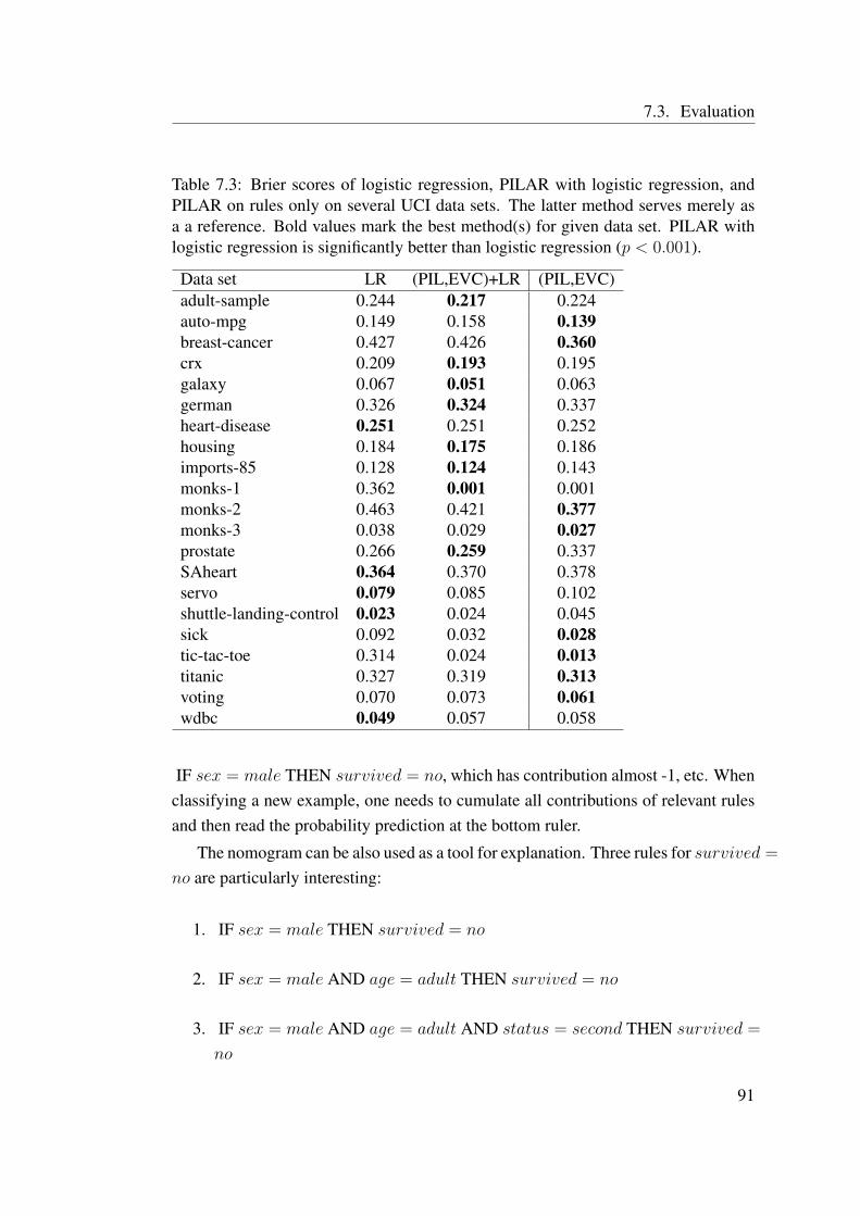
7.3. Evaluation
Table 7.3: Brier scores of logistic regression, PILAR with logistic regression, andPILAR on rules only on several UCI data sets. The latter method serves merely asa a reference. Bold values mark the best method(s) for given data set. PILAR withlogistic regression is significantly better than logistic regression (p < 0.001).
Data set LR (PIL,EVC)+LR (PIL,EVC)adult-sample 0.244 0.217 0.224auto-mpg 0.149 0.158 0.139breast-cancer 0.427 0.426 0.360crx 0.209 0.193 0.195galaxy 0.067 0.051 0.063german 0.326 0.324 0.337heart-disease 0.251 0.251 0.252housing 0.184 0.175 0.186imports-85 0.128 0.124 0.143monks-1 0.362 0.001 0.001monks-2 0.463 0.421 0.377monks-3 0.038 0.029 0.027prostate 0.266 0.259 0.337SAheart 0.364 0.370 0.378servo 0.079 0.085 0.102shuttle-landing-control 0.023 0.024 0.045sick 0.092 0.032 0.028tic-tac-toe 0.314 0.024 0.013titanic 0.327 0.319 0.313voting 0.070 0.073 0.061wdbc 0.049 0.057 0.058
IF sex = male THEN survived = no, which has contribution almost -1, etc. Whenclassifying a new example, one needs to cumulate all contributions of relevant rulesand then read the probability prediction at the bottom ruler.
The nomogram can be also used as a tool for explanation. Three rules for survived =
no are particularly interesting:
1. IF sex = male THEN survived = no
2. IF sex = male AND age = adult THEN survived = no
3. IF sex = male AND age = adult AND status = second THEN survived =
no
91

7. CLASSIFICATION FROM RULES AND COMBINING ABCN2 WITH OTHER
METHODS
Figure 7.2: A nomogram visualising weighted rule’s model for Titanic domain.
All three rules have contribution around -1. According to these rules, being a malewas tough when the accident happened. However, being a male and also an adultwas even worse. Note that being an adult by itself was not necessarily bad, otherwisesuch rule would be in the model. Furthermore, an adult male from the second classstood the least chances for survival.
92
7.4. PILAR + any method = any ABML method
7.4 PILAR + any method = any ABML method
PILAR can be used as a simple bridge between argument based knowledge and anymachine learning method. We start with learning rules from argumented examplesin Algorithm 5.2, but then skip the last part where rules are learned with the stan-dard CN2ForOneClass. Afterwards, we can choose any machine learning algorithmto learn a model and use PILAR to combine this model with rules. The resultingmodel is based on the chosen learning algorithm corrected with the rules learnedfrom argumented examples.
Although this simple algorithm can be seen as an argument-based generalisationof all machine learning algorithms, we believe that it can not replace actual extensionsof these algorithms. These rules learned from arguments can only slightly correctthe base model in some local spots, whereas an AB-extension of the method wouldactually learn a completely different model.
7.5 Discussion
PILAR is foremost a method for classification from rules. It combines rules witha weighted linear sum, where weights are automatically learned from learning data.Additionally, PILAR also allows improving probabilistic prediction of other proba-bilistic machine learning methods. Rules are used as constraints on the final model,requiring that its probabilistic predictions are on average similar to the probabilisticestimates given by rules.
We studied the usefulness of our method as a rule classification technique andas a correction method for logistic regression. In both cases, PILAR proved to bea promising method and statistically outperformed competing methods. Given ourexperimental findings, we believe that it would improve (or at least not worsen) anygeneral classification method. Furthermore, PILAR also preserves the splendid ex-planation property of rules, e.g. their weights could be visualised in a nomogram.
There already exist some approaches that combine linear classifiers (e.g. logis-tic regression) with non-linear (decision trees) [LHF03]. While these approaches areconceptually different from ours, it would be still interesting to explore, if it is, on av-erage, better to correct a linear classifier with rules or induce one model that containsboth ideas.
93

Chapter 8
ABML Refinement Loop: Selection ofCritical Examples
In ABML experts are asked to provide their prior knowledge in the form of argumentsfor specific learning examples rather than the general domain knowledge. However,asking experts to give arguments for the whole learning set is not likely to be feasible,because it would require too much time and effort. The following loop describes theskeleton of the procedure that picks out critical examples - examples that ABML cannot explain without some help:
1. Learn a hypothesis with ABML using given data.
2. Find the most critical example and present it to the expert. If a critical examplecan not be found, stop the procedure.
3. Expert explains the example; the explanation is encoded in arguments and at-tached to the learning example.
4. Return to step 1.
To finalize the procedure we need to contemplate the following two questions:
• How do we select critical examples ?
• How can we achieve to get all necessary information for the chosen example?
95
8. ABML REFINEMENT LOOP: SELECTION OF CRITICAL EXAMPLES
8.1 Identifying critical examples
The main property of critical examples is that the current hypothesis can not explainthem very well, or in other words, it fails to predict their class. Since ABCN2 givesprobabilistic class prediction, we define the most critical example as the examplewith the highest probabilistic error. The probabilistic error can be measured in severalways. One possibility is to learn a hypothesis on the whole set and test on the sameset, although, if the method is prone to overfitting, not many critical examples are tobe found. Therefore, we propose the k-fold cross-validation repeated n times (e.g.n = 4, k = 10), so that each example is tested n times. The most critical example isthus the one with highest average probabilistic error.
The selection of the most mispredicted example as the one being shown to theexpert has a possible deficiency. It is not always true that this example will benefitthe most to the quality of the next learned hypothesis. For instance, the examplecould be an outlier, where the probability of encountering a similar example is small.Therefore, the argument would improve classification of this example only and noneother.
This suggests a selection of a critical example that would, after being argumented,increase the most the quality (e.g. accuracy) of the learned hypothesis. Having aprocedure able to do exactly this, we could expect a smaller number of iterationsrequired to reach the best possible hypothesis, hence, reducing the overall time of ex-pert’s involvement in the process. A possible approach would be to apply a clusteringalgorithm[JMF99] on all critical examples and choose an example from a large clus-ter. An argument for this example is likely to help also other examples in the samecluster. Another approach could be to try a mechanism for outlier detection[HA04].If an example is an outlier, there is not much chance that the expert will be able toprovide good arguments, and more, such arguments are unlikely to help other crit-ical examples. Note that a similar problem has been raised several times in activelearning, see for instance [MN98; NS04]. However, by now we were not yet ableto develop a credible algorithm for this task, therefore the question is still open forfuture work.
96

8.2. Are expert’s arguments good or should they be improved?
8.2 Are expert’s arguments good or should they beimproved?
Here we describe in detail the third (3) step of the above algorithm, where the expertis asked to explain the critical example. The provided arguments can be complete- they perfectly explain the example - or incomplete. In the former case, the expertprovided all relevant information and the process can move to the next step. If ar-guments are incomplete, then ABML will sometimes be able to explain the exampleusing arguments and inducing the incomplete part, while sometimes this will still notbe entirely possible. In such cases, we need additional information from the expert.The whole procedure for one-step knowledge acquisition is described with the next5 steps:
Step 1: Explaining critical example. In this step the expert is asked the followingquestion: ”Why is this example in the class as given?” Her answer can beeither ”I don’t know” (she is unable to explain it) or she can articulate a set ofarguments A1, . . . , Ak all confirming the example’s class value. If the systemgets the first answer, it will stop this procedure and try to find another criticalexample.
Step 2: Adding arguments to the example. ArgumentsAi are given in natural lan-guage and need to be translated into domain description language (attributes).Each argument supports its claim with a number of reasons. When a reasonis simply an attribute value of the example, then the argument can be directlyadded to example. On the other hand, if reasons mention other concepts, notcurrently present in the domain, these concepts need to be included in the do-main before the argument can be added to the example.
Step 3: Discovering counter examples. Counter examples are used to spot if argu-ments are enough to successfully explain the critical example or not. If ar-guments are incomplete and ABML fails to improve them, then the counterexamples will show where the problem is. Here, ABML is first used to inducea hypothesis H1 using data without new arguments and H2 using data togetherwith the new arguments. A counter example is defined as: it has a differentclass value from the critical example, its probabilistic error increases in H2
with respect to H1, and H2 mentions arguments (given to the critical example)while explaining the counter example.
97
8. ABML REFINEMENT LOOP: SELECTION OF CRITICAL EXAMPLES
Step 4: Improving arguments. The experts needs to revise her initial argumentswith respect to the counter example. This step is similar to steps 1 and 2 withone essential difference; the expert is now asked ”Why is the critical examplein one class and the counter example in the other?” The answer is added to theinitial argument.
Step 5: Return to step 3 if counter example found.
8.3 Similarity and differences with active learning
Active Learning is a type of machine learning where the learning method has certaincontrol over the selection of learning examples. It is assumed that all possible exam-ples are initially unclassified, and the learning method gradually selects examples,which get classified by an expert, and are then used in learning. The approach isespecially useful in domains where labeling (assigning class values) to an arbitraryexample takes a lot of time or/and is expensive. A good active learning method is onethat selects as few learning examples as possible and reaches acceptable accuracy.
The standard loop in active learning consists of the following steps:
1. Select randomly k initial learning examples from the set of unclassified exam-ples and obtain their class values. These examples represent the current set ofclassified examples E.
2. Learn a classifier C given E.
3. Select the most valuable example e (that would improve C the most if addedto E) from the remaining unclassified examples .
4. Obtain class value of e, add it to the set of examples E, and return to step 2.
Different methods in active learning use different strategies to select examples in step3.
The ABML refinement loop described in the previous sections appears similarto the loop of active learning. In each turn they both add information to the learn-ing set of examples; in ABML, additional arguments for an example are provided,while in active learning a new example is classified and appended to the learning set.However, although they are similar, they are also very different. In ABML, we as-sume that all classes of examples are known, but the method can not explain some of
98
8.3. Similarity and differences with active learning
them, therefore needs additional knowledge to explain them. On the other hand, ac-tive learning does not know the class values and searches for an example that wouldimprove the learned hypothesis the most. This difference also necessarily definesdifferent strategies that the approaches adopt. In the argument based machine learn-ing loop, we try to find an example that poses the greatest problems for the learningmethod, while in active learning we select an unclassified example where the currentclassifier is the least certain how to classify. Common to both approaches is the de-sire to find an example with large area of effect - adding information to that examplewould increase the accuracy of model the most. We shall quickly review some basicapproaches to active learning (a more comprehensive review can be found in [Set09])and show how and if their ideas are suitable to be used within the ABML loop. Aswe shall see, all methods have limited (if any) usability for the ABML loop.
Uncertainty sampling
In uncertainty sampling, the method selects the example for which the current clas-sifier is the least certain [LA94], since it assumes that this and similar examplesare therefore not represented enough in the learning set. For example, if we havea probabilistic classifier and a two-class problem, then the method would select theunclassified example where the prediction was closest to 0.5.
This approach is intuitive in active learning, however its usefulness in argumentmachine learning is unclear. Asking an expert to provide arguments for an examplewhere the method is the least certain would improve the quality of hypothesis, as theexample is still problematic. Nevertheless, such an example is less critical than theone with the highest probabilistic error. Moreover, there seems to be no mechanismto select an example with largest area of effect. Hence, we expect that selection ofcritical examples following this strategy would require more steps in ABML.
Query by committee
Here, we first learn a set of classifiers using different machine learning methods.These classifiers are then tested on unclassified examples. The method selects theexample where these classifiers disagreed the most [SOS92].
This is a similar method to uncertainty sampling. It has the same deficienciesfor ABML loop: example where all classifiers are wrong would be a better selectionmethod and there are no guidelines how to select an example with largest area ofeffect.
99

8. ABML REFINEMENT LOOP: SELECTION OF CRITICAL EXAMPLES
Version space reduction
This principle is described in [CAL94] and it works only for binary classes. The ideais to learn two models from all examples, the most general, and the most specificconsistent classifier in the given version space [Mit97]. Consistency is defined asusual as 100% classification accuracy on learning data. The method then selects anexample from the unclassified set, where these two models disagree.
This approach could be also applied in the ABML loop. The example that wouldbe differently classified by the most general and the most specific hypothesis (exam-ple would be before removed from learning set), would be shown to an expert forexplanation. However, since version spaces assume noise-free domains, its applica-bility to real domains is questionable.
Future error reduction
The idea of this method, sometimes referred to also as “estimated error reduction”,is to select an example that will the most reduce the prediction error of the classi-fier [RM01]. The selection procedure builds several models from the current learningset extended by one unclassified example, which is labeled into one of the possibleclass values. The selected example is the one that would, on average over all assignedclasses, minimise the expected error on all testing examples.
This principle would in ABML be translated to: select such an example thatwould, if argumented, the most reduce the error of the method. This sounds nice, es-pecially since it would implicitly avoid selecting outliers as critical examples. How-ever, while learning models for all possible classes for all unclassified examples ispossible, learning over all possible arguments is not, since the number of all possiblearguments is usually very large.
Density-weighted methods
This approach [SC08] was designed to directly deal with the problem of outliers.The main idea is that informative instances should not only be those which are un-certain, but also those which are “representative” of the input distribution (i.e., inhabitdense regions of the input space). Such methods still suffer from the same dilemma(knowing class values vs. not knowing class values), however, the combination ofthe method for finding the most critical example together with the method for findinga representative example seems very promising.
100

Part III
Experiments and Evaluation
101

Chapter 9
Introductory experiments
In this last part of the Thesis, we will describe several applications and experimentswhere ABCN2 was involved. These experiments will be used to demonstrate thefunctionality of ABCN2 and to compare the results of learning with or without ar-guments. They will also illustrate the argument based machine learning loop that isswitching between learning and querying domain experts. Furthermore, these exper-iments shall also be used as an evaluation of the ABCN2 method. A problem withevaluation is that a statistical comparison of ABCN2 and other (non-abml) methods isvirtually impossible. As each experiment involves asking domain experts questionsabout the domain, which requires some of their time, these experiments can relativelytake a lot of time (they can not be run automatically). For this reason, we can do onlya smaller number of experiments and in each of them qualitatively answer some ofthe following questions:
• Does learning with arguments provide favorable hypotheses in comparisonwith learning without arguments? When should we prefer one or the other?This will be measured in terms of accuracy and comprehensibility of learnedhypotheses.
• How effective is the method for selection of critical examples, that is, howwell does this mechanism guide the expert’s attention to important cases andmissing information?
• How difficult is it for the experts to provide their prior knowledge in the formof arguments?
103

9. INTRODUCTORY EXPERIMENTS
• Can we efficiently reconstruct an existing knowledge base? Is it possible touse an existing knowledge base as a source of arguments, where the result oflearning is then an updated knowledge base?
• What if the explanation of examples does not mention the attributes describingthe example? We will see that arguments can also suggest new attributes.
• Can relevant arguments be extracted automatically from relevant literature,rather than provided by an expert?
• What if arguments provided are not perfectly correct? What if the argumentsare not correct at all - how to deal with noise in experts’ knowledge?
We split the evaluation to four chapters. The present one will describe four ex-periments with ABCN2 to illustrate the core idea of ABCN2: learning to classify an-imals, an experiment using the “South African Heart disease” UCI domain [AN07],an application to a legal domain, and an application to prognosis of bacterial infec-tions in geriatric population. All four experiments are basic by nature. They do notrequire any special handling with arguments, where arguments are provided by anexpert and are simply conjunctions of available attributes. In the following chapter,we will describe some experiments where arguments do mention only available at-tributes, but also others yet not present in the domain or a combination of currentattributes that can not be easily expressed with a conjunction of reasons. The nextchapter will demonstrate how relevant arguments can be extracted from text sourcesand how helpful are they. In the last chapter of this part, we will cope with theproblem of erroneous arguments and how prone is ABCN2 to these errors.
9.1 Animal classification
The ZOO data set [AN07] contains descriptions of 101 animals (instances) with 17attributes: hair, feathers, eggs, milk, predator, toothed, domestic, backbone, fins, legs,tail, catsize, airborne, aquatic, breathes, venomous, and type, which is the classattribute. Type has seven possible values: mammal, bird, reptile, fish, amphibian,insect, and other. The main advantage of this data set is that, just using an encyclo-pedia, we can provide good arguments to automatically selected critical examples.We expect that using arguments will help to improve the comprehensibility and clas-sification accuracy of induced rules.
104
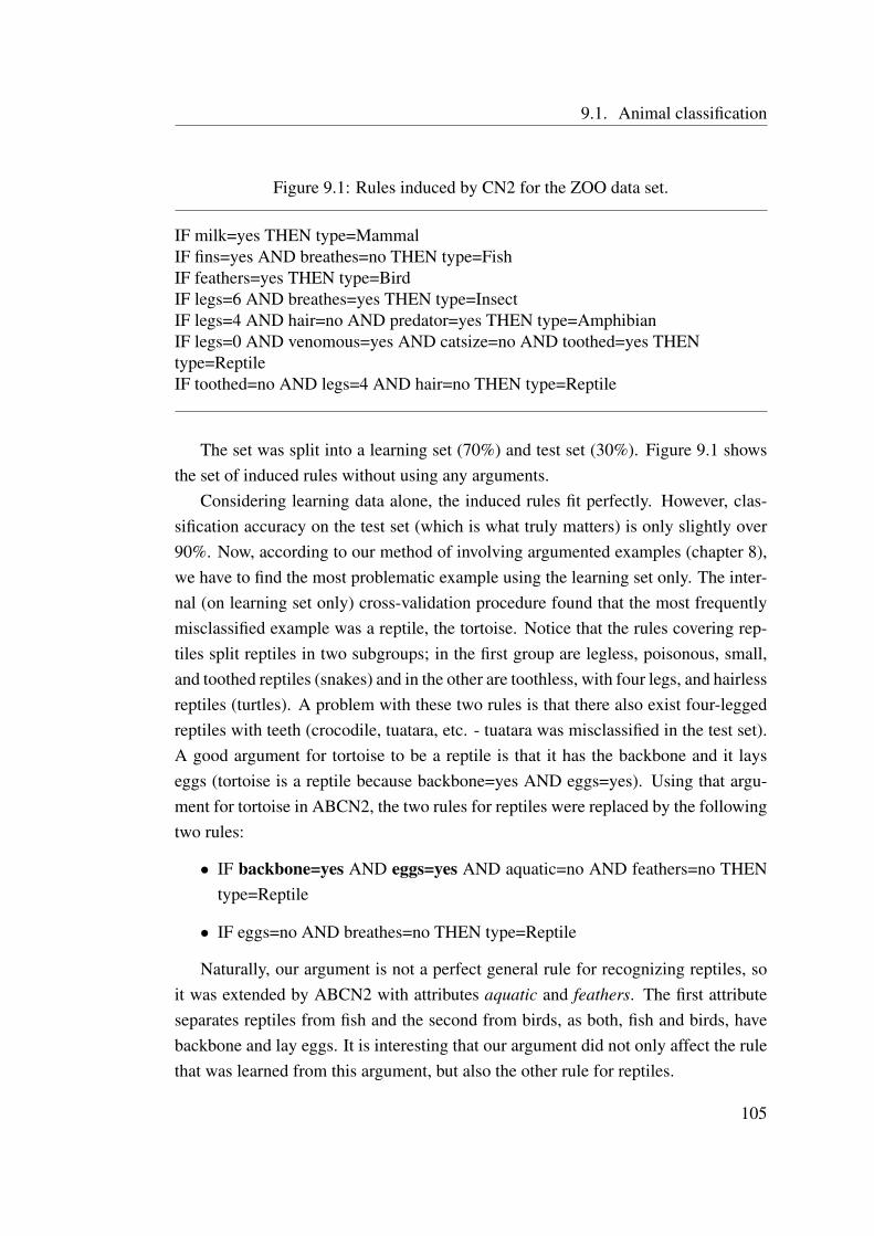
9.1. Animal classification
Figure 9.1: Rules induced by CN2 for the ZOO data set.
IF milk=yes THEN type=MammalIF fins=yes AND breathes=no THEN type=FishIF feathers=yes THEN type=BirdIF legs=6 AND breathes=yes THEN type=InsectIF legs=4 AND hair=no AND predator=yes THEN type=AmphibianIF legs=0 AND venomous=yes AND catsize=no AND toothed=yes THENtype=ReptileIF toothed=no AND legs=4 AND hair=no THEN type=Reptile
The set was split into a learning set (70%) and test set (30%). Figure 9.1 showsthe set of induced rules without using any arguments.
Considering learning data alone, the induced rules fit perfectly. However, clas-sification accuracy on the test set (which is what truly matters) is only slightly over90%. Now, according to our method of involving argumented examples (chapter 8),we have to find the most problematic example using the learning set only. The inter-nal (on learning set only) cross-validation procedure found that the most frequentlymisclassified example was a reptile, the tortoise. Notice that the rules covering rep-tiles split reptiles in two subgroups; in the first group are legless, poisonous, small,and toothed reptiles (snakes) and in the other are toothless, with four legs, and hairlessreptiles (turtles). A problem with these two rules is that there also exist four-leggedreptiles with teeth (crocodile, tuatara, etc. - tuatara was misclassified in the test set).A good argument for tortoise to be a reptile is that it has the backbone and it layseggs (tortoise is a reptile because backbone=yes AND eggs=yes). Using that argu-ment for tortoise in ABCN2, the two rules for reptiles were replaced by the followingtwo rules:
• IF backbone=yes AND eggs=yes AND aquatic=no AND feathers=no THENtype=Reptile
• IF eggs=no AND breathes=no THEN type=Reptile
Naturally, our argument is not a perfect general rule for recognizing reptiles, soit was extended by ABCN2 with attributes aquatic and feathers. The first attributeseparates reptiles from fish and the second from birds, as both, fish and birds, havebackbone and lay eggs. It is interesting that our argument did not only affect the rulethat was learned from this argument, but also the other rule for reptiles.
105

9. INTRODUCTORY EXPERIMENTS
The next problematic example found was a sea snake (a reptile). A sea snake isan air-breathing snake that lives underwater. According to encyclopedia, a sea snakeshould be correctly classified with the above rule, however we noticed that, in thedata, sea snake is characterized as a non-breathing reptile and that it does not layeggs. It is obviously a mistake in data and is also the reason for the induction ofthe second rule. It is interesting to note how the interactive use of our AB learningmethod also helps to identify errors in data.
The next problematic example found in the learn set was a newt. The argumentwas provided that the newt is an amphibian because it has backbone, lays eggs and isrelated to water. This resulted in the rule:
IF backbone=yes AND aquatic=yes AND eggs=yes AND legs=4THEN type=Amphibian
After adding these arguments to the two examples, ABCN2 induced a perfect setof rules for the ZOO data set. There were no misclassified examples in the test set.
This example clearly illustrates the effectiveness of our method for choosing crit-ical examples (both identified examples were really critical) and shows how argu-ments can be used to learn concepts that are otherwise very hard to learn. The exam-ple also nicely illustrates that it is much easier to give arguments only to an individualexample (e.g why tortoise is a reptile), than it would be to articulate general rulesthat correctly classify the animals. Moreover, the rules learned from arguments areconsistent with prior knowledge and the resulting hypothesis achieved higher classi-fication accuracy than the initial (learning without arguments) one.
9.2 Welfare benefit approval
In this section, we shall describe an experiment in a domain of law published in oneour earlier papers [MvBC+06]. At that time, we had not yet developed EVC andPILAR (Chapters 6 and 7), therefore the ABCN2 in this section uses the originalCN2’s classification and rule evaluation.
The problem of many areas of law - especially administrative law - is that manycases are routinely decided, which often involve the exercise of some discretion, orinvolve some degree of operationalisation of the concepts used in the legislation:for example aged over 65 rather than elderly [BC91b]. We would generally wish to
106

9.2. Welfare benefit approval
assume that such discretion or operationalisation is consistent so that like cases aredecided in a like manner, that some kind of rule is being followed.
We would like to analyse if there is a way of deciding what the rule being followedis from an automated consideration of the data. Such a question has relevance to anumber of interesting and important issues:
• If there is well defined legislation which defines what the rule should be wemay wish to ensure that the rule is being followed;
• If the domain is a discretionary one, we may wish to discover the rule itself;
• Similarly, we may wish to discover the way in which the stated conditions havebeen operationalised;
• Some people have argued that the rule followed in practice is different fromthe rule which exists in theory (or which might be elicited from experts). Forexample Edwards [Edv95] suggested that some areas of law exhibited a sys-tematic bias. Such conjectures could be informed and justified were we able todiscover the ”real” rule from a database recording the actual practice.
If therefore we had a reliable technique to extract rules explaining the data in afield of law, it would have many interesting uses.
One problem with many experiments to explore the efficacy of techniques de-signed to extract knowledge from data is that they use data for which the relationshipspresent are not known at the outset. As a result, what has been discovered, and whathas been missed, cannot be established definitively. Often accuracy of classificationis taken to validate the knowledge extracted, but this test is, as will be discussed be-low, rather one-sided. In the work reported here we will use a specially constructeddata set, the properties of which are known, and which is thus able to serve as ameasurable test of the technique.
The data we use has been used in several previous AI and Law experiments, re-ported in [BC93; BCC00; JG03]. The use of this same data set allows for comparisonbetween what can be derived using the various techniques.
9.2.1 The data set
As previously mentioned the data set used in these experiments is that first usedin [BC93]. The data concerns a fictional welfare benefit. The benefit is payable if six
107
9. INTRODUCTORY EXPERIMENTS
conditions are satisfied. These conditions were chosen to represent different kinds ofcondition that are found in the legal domain, so that we can see whether the differentform of conditions affects their discoverability.
The notional benefit was a fictional welfare benefit paid to pensioners to defrayexpenses for visiting a spouse in hospital. The conditions were:
1. The person should be of pensionable age (60 for a woman, 65 for a man);
2. The person should have paid contributions in four out of the last five relevantcontribution years;
3. The person should be a spouse of the patient;
4. The person should not be absent from the UK;
5. The person should have capital resources not amounting to more than 3,000;
6. If the relative is an in-patient the hospital should be within a certain distance:if an out-patient, beyond that distance.
These conditions represent a range of typical condition types: 3 and 4 are Booleannecessary conditions, one which should be true and one false; 5 is a threshold on acontinuous variable representing a necessary condition, and 2 relates five Booleanvariables, only four of which need be true. 1 and 6 relate the relevance of one variableto the value of another: in 1 sex is relevant only for ages between 60 and 65, andin 6 the effect of the distance variable depends on the Boolean saying whether thepatient is an in-patient or an out-patient. We can see these six conditions eitheras explicit conditions or as ways of making operational concepts such as elderly,sufficient contribution record, close relative, presence in the UK, insufficient capitalresources, and attributable expenses respectively.
A possible criticism of this experiment could be based on the fact that our ex-perimental data was artificial rather than real world. However, in machine learningexperimentation with artificial data is quite common and acceptable in testing ma-chine learning methods. It has the advantage over the use of real-world data in thatthe experiment is better controlled and the success of learning is easier to assess.Moreover, the underlying rules used to generate the synthetic data were not told be-forehand to those conducting experiments with ABCN2, but were known only to thedata owner (Trevor Bench-Capon).
108

9.2. Welfare benefit approval
For this experiment a data set of 2400 records was used: 1200 satisfying all of theconditions, and equal numbers of the remainder being designed to fail. For recordsdesigned to fail one of the conditions, satisfaction or otherwise of the remaining con-ditions was decided randomly for each condition separately. There are thus twelveattributes relevant to the decision: age, sex, the five contribution conditions (calledcont5, cont4, cont3, cont2 and cont1), spouse, absent, capital, distance and inpatient.In addition to these attributes each record contains fifty two irrelevant attributes, halfof which are continuous and half Boolean. An ideal set of rules would be:
1. IF age < 60 THEN qualified = no;
2. IF age < 65 and sex = m THEN qualified = no;
3. IF any two of cont5, cont4, cont3, cont2 and cont1 = nTHEN qualified = no;
4. IF spouse=no THEN qualified=no;
5. IF absent=yes THEN qualified=no;
6. IF capital>3000 THEN qualified=no;
7. IF inpatient=yes AND distance> 750 THEN qualified=no;
8. IF inpatient=no AND distance≤ 750 THEN qualified=no;
Probably we should expect (3) to be expressed as ten separate rules containingeach pair of the contribution factors, which would be a total of sixteen rules to de-scribe the problem fully.
9.2.2 Experiment with ABCN2
To evaluate the results produced by ABCN2, we split the original data (2400 records)into a learning set containing 70% of the cases, and a test set (the remaining 30%)used to assess the accuracy of the generated rules on new cases. The random selectionwas stratified to pertain the class distribution.
The first set of rules was generated from examples without any arguments. So theresulting rules were as if generated with CN2. These rules were:
1. IF capital > 2900 THEN qualified = no;
109

9. INTRODUCTORY EXPERIMENTS
2. IF age ≤ 59 THEN qualified = no;
3. IF absent = yes THEN qualified = no;
4. IF spouse = no THEN qualified = no;
5. IF cont4 =no AND cont2 = no THEN qualified=no;
6. IF age > 89 THEN qualified = no;
Of these (1) - (5) are correct (or very close). Nine contributions rules and the twodistance rules are missing and rule (6) is wrong. There is thus considerable scopefor improvement. None the less a high degree of accuracy is achieved by these sixrules: 99% for both the learning and the test sets. Accuracy of classification is not,however, of prime interest: the motivations given at the beginning of section make itclear that it is the interpretability of the rules discovered that is of primary interest.
After inducing these rules with CN2, our plan was to give arguments to someof the examples in the learning set and using ABCN2 to induce better rules. In thecase of our legal data, the procedure for finding the most critical example founda misclassified example that failed on the contributions condition. The argumentgiven for this example was that cont5, cont4 and cont1 are all false. When thisargumented example, together with all the other (non-argumented) examples wasgiven to ABCN2, two additional contribution rules were induced:
IF cont5 = no AND cont4 = no AND cont1 = no
THEN qualified = no;
IF cont2 = no AND cont3 = no THEN qualified = no;
and the accuracy increased slightly.
In a third learning iteration, an argument was added to an additional misclassifiedcase in which distance was too great for an inpatient. This time the erroneous rule (6)disappeared and was replaced by a rule relating to inpatiency and distance (althoughwith an approximate threshold) and another contributions rule:
IF inpatient = yes AND distance > 735 THEN qualified = no;
IF cont1 = no AND cont5 = no THEN qualified = no;
110

9.2. Welfare benefit approval
Iterations four, five and six added three more arguments based on failure of thecontribution conditions, which resulted in a different contributions rule. In iterationseven, the argument was given that distance was too small for outpatient. This pro-duced the rule
IF inpatient = no AND distance ≤ 735 THEN qualified = no;
and rearranged the contribution rules somewhat.At this point there were no critical examples found any more, and so no further
argumentation with our iterative procedure was possible. The final accuracy on thetest set was 99.8%. This means that one out of 720 test cases was misclassified, andall the rest were classified correctly. The final set of rules were:
1. IF capital > 2900 THEN qualified = no;
2. IF age ≤ 59 THEN qualified = no;
3. IF absent = yes THEN qualified = no;
4. IF spouse = no THEN qualified = no;
5. IF cont4 = no AND cont2 = no THEN qualified = no;
6. IF inpatient = yes AND distance > 735.0 THEN qualified = no;
7. IF inpatient = no AND distance ≤ 735 THEN qualified = no;
8. IF cont3 = no AND cont2 = no THEN qualified = no;
9. IF cont5 = no AND cont3 = no AND cont1 = no
THEN qualified = no;
10. IF cont4 = no AND cont3 = no AND cont1 = no
THEN qualified = no;
11. IF cont5 = no AND cont4 = no AND cont1 = no
THEN qualified = no;
(1) - (5) are all good rules and remain from the first pass. (6) and (7) havethe right format, but the threshold is slightly inaccurate. The remaining four rulesapproximate the ten ideal contribution rules. The total number of argumented ex-amples after the seven iterations was seven. The one misclassified example was
111

9. INTRODUCTORY EXPERIMENTS
(omitting the irrelevant attribute values): ((age = 84, sex = male, cont1 = no,cont2 = yes, cont3 = no, cont4 = yes, cont5 = yes, spouse = yes, absent = no,capital = 130, distance = 1320, inpatient = no), qualified = no). This exampleis misclassified because the particular combination of contribution conditions is notcovered by the approximate contribution rules induced.
Learning from artificial data sets is usually considered easier than learning fromreal world data sets. One reason for this is that artificial data are typically noise-freewhereas real world data typically contain noise. So to cope with real world data, alearning method has to be able to deal with noise. To analyse the ABCN2’s abilityto deal with noise in data, we artificially introduced random noise of varying severityin our learning data as described below. Intuitively we expected that backgroundknowledge in the form of arguments should improve the method’s resistance to noisein comparison with CN2. This expectation was confirmed by the experiments.
The experimental procedure for this experiment was as follows. First, we splitthe data set to learning set (70%) and test set (30%). Then we added random noiseinto the learning set, induced rules with both CN2 and ABCN2, and measured theaccuracy of both sets of rules on the (noise-free) test set. To study how the severityof noise affects the success of learning, we repeated the experiment for various ratesof noise. The chosen rates were: 0%, 2%, 5%, 10%, 20%, and 40%. A noise rate pmeans that with probability p the class value of each learning example is replaced bya random value drawn from {yes, no}with distribution (0.5, 0.5). Each time CN2 andABCN2 were run with correspondingly ”noised” examples plus the same noise-freeargumented examples defined above. This whole procedure was repeated 10 times inorder to obtain confidence intervals of the estimated average classification accuracyfor both CN2 and ABCN2 for each noise rate.
Figure ?? and Table 9.1 show the results of CN2 and ABCN2. Both methods wererun with the default settings of their parameters. These standard values are: m=2 inm-estimate, α=0.001(likelihood ratio statistics threshold), and minimal coverage ofa rule is set to 2 (that is, a rule to be acceptable has to cover at least two examples).
This figure shows that, as expected, ABCN2 clearly outperforms CN2 when rateof noise in data increases. The difference in average accuracies between ABCN2and CN2 jumped from 0.3% at 0% noise to 3.3% at 20% and to 1.7% at 40% noise.ABCN2 outperformed CN2 on 0%, 20%, and 40% noise with high statistical signif-icance (t-test,p<0.001; see Table 9.1). ABCN2 was also the better method for othernoise rates but with lower significances.
The ability to handle a large amount of noise is very important in the kind of rou-
112

9.2. Welfare benefit approval
0% 2% 5% 10% 20% 40%
noise rate
0.8
0.9
1.0
CA
××
×
×
×
×
••
•
•
•
•
. . . . . . . . . . . . . . . . . . . . . . . . . . . ..........................
.......................................................................................................................................................................................................................................................................................................................................................................................................................................................................................................................................................................................................................................................................
CN2 ×ABCN2 •
Figure 9.2: CN2 and ABCN2 compared on learning data sets with different propor-tions of noise in class variable.
noise CN2 ABCN2 Sig.0% 0.9947±0.0010 0.9976±0.0005 <0.0012% 0.9778±0.0030 0.9842±0.0020 0.0025% 0.9636±0.0034 0.9696±0.0017 0.00510% 0.9351±0.0053 0.9469±0.0051 0.03720% 0.8869±0.0079 0.9200±0.0056 <0.00140% 0.8326±0.0068 0.8503±0.0088 0.001
Table 9.1: Results of CN2 and ABCN2 on noisy data. The first column shows noiserates, second and third contain average accuracy and standard error of accuracy es-timate for CN2 and ABCN2 respectively, and the last column gives significances ofdifferences between averages computed with pairwise t-test.
113

9. INTRODUCTORY EXPERIMENTS
tine legal decision making we are addressing. Errors rates are very high: Groothuisand Svenson[GS00] report experiments which suggest that 20% may be a low esti-mate of incorrectly decided cases. The problem is internationally widespread. TheUS National Bureau of Economic Research reports of a particular benefit∗:
“The multistage process for determining eligibility for Social Secu-rity Disability Insurance (DI) benefits has come under scrutiny for thelength of time the process can take - 1153 days to move through theentire appeals process, according to a recent Social Security Administra-tion (SSA) analysis - and for inconsistencies that suggest a potentiallyhigh rate of errors. One inconsistency is the high reversal rate during theappeals process - for example, administrative law judges, who representthe second level of appeal, award benefits in 59% of cases. Another in-consistency is the variation in the award rates across states - from a highof 65% in New Hampshire to a low of 31% in Texas in 2000 - and overtime - from a high of 52% in 1998 to a low of 29% in 1982.”
Again an official UK Publication produced by the Committee of Public Ac-counts†:
“Finds that the complexity of the benefits system remains a majorproblem and is a key factor affecting performance. Skills of decision-makers need to be enhanced through better training and wider experi-ence. Too few decisions are right first time, with a error rate of 50%for Disability Living Allowance. There are also regional differences indecision making practices that may lead to payments to people who arenot eligible for benefits.”
This makes it clear that robustness in the face of large amounts of noise is essen-tial if a learning techniques is to be applied to data from this domain.
9.2.3 Discussion
In this experiment, we found that ABCN2 performed a little better than CN2 in termsof accuracy - which is very well indeed. However, the quality, in terms of inter-
∗From Web Page: http://www.nber.org/aginghealth/winter04/w10219.html†Getting it right: Improving Decision-Making and Appeals in Social Security Benefits. Commit-
tee of Public Accounts. London: TSO, 2004 (House of Commons papers, session 2003/04; HC406)
114
9.3. Infections in elderly population
pretability, of the rules generated showed a crucial advantage of ABCN2. The argu-ment based machine learning loop enabled adding domain knowledge in the form ofthe justification of particular decisions, and this was able to give a great improvementto the quality of the rules. Additionally, we explored the robustness of ABCN2 in theface of erroneous decisions. It was found in the experiment that ABCN2 is morerobust against noise than its non-argument original CN2. This is important becausemany of the administrative law applications to which we would wish to apply thetechnique exhibit quite large error rates [GS00].
9.3 Infections in elderly population
In this section, we will describe an application of ABCN2 to a medical domain [vMVB06].The particular problem is to build a model from data which would help the physician,at the first examination of an older patient with an infection, to decide the severity ofthe infection and consequently, whether the patient should be admited to the hospitalor could be treated as an outpatient.
The elderly population is a unique one and that is also true from the medicalperspective. Compared to younger population, people over 65 years of age usuallyreact to a disease in a different way. Many symptoms may not even be present orthey are masked by others which makes it a very difficult task for a medical doctorto diagnose a condition, to decide a proper treatment or to estimate the patient’srisk of death. From a wider perspective, the proportion of elderly in the populationis growing rapidly and so are the costs for medical treatment, which presents anemerging economic problem.
9.3.1 Data
The data for our study was gathered at the Clinic for Infectious Diseases in Ljubljana,from June 1st, 2004 to June 1st, 2005. The physicians included only the patients over65 years of age with CRP value over 60 mg/l, which indicated a bacterial etiology ofthe infection. The patients were observed 30 days from the first examination or untildeath caused by the infection. The data includes 40 clinical and laboratorial parame-ters (attributes) acquired at the first examination for each of 298 patients (examples).The infections are distinguished with respect to the site where bacteria is found oron the clinical basis (respiratory, urinary tract, soft tissues, other). The continuous
115

9. INTRODUCTORY EXPERIMENTS
attributes were categorized by the physician. The distribution of the class attributedeath (whether death has occurred or not) is the following:
• 34 examples (11,4%) for ’death = yes’
• 263 examples (88,6%) for ’death = no’
9.3.2 Arguments
Attribute ValueGENDER Z Positive argumentsAGE YEARS 92AGE C DEATH=YES because RESPIRATORY RATE D=“>= 16”NURSING HOME RESIDENT NO DEATH=YES because SATURATION D=“<= 90”COMMORBIDITY 0 DEATH=YES because BLOOD PRESSURE D=”<= 100”DIABETES NO DEATH=YES because TEMPERATURE D=“> 37.9”HEART NO DEATH=YES because LEUKOCYTES D=“>= 12”KIDNEY NO DEATH=YES because CREATININE D=“>= 100”LIVER NO DEATH=YES because BLOOD UREA D=“>= 13”LUNG NO DEATH=YES because NA D=“> 147”IMMUNITY NO DEATH=YES because AGE YEARS is highCENTRAL NERVE SYSTEM NO DEATH=YES because WEAKNESS=YESMOBILITY YES DEATH=YES because CONSCIOUSNESS=DISSORIENTEDCONTINENCE YESBEDSORE NO Negative argumentsCATHETER NOIMPLANT NO DEATH=YES despite MOBILITY=YESVOMITING NO DEATH=YES despite CONTINENCE=YESDIABLOODPRESSUREHEA NO DEATH=YES despite TROMBOCYTES D=“>= 100”WEAKNESS YES DEATH=YES despite HEART RATE D=“< 100”CONSCIOUSNESS DISSORIENTED DEATH=YES despite RODS D=“< 10”TROMBOCYTES D >= 100 DEATH=YES despite CRP D=“< 150”TEMPERATURE D > 37.9 DEATH=YES despite COMMORBIDITY=0RESPIRATORY RATE D >= 16SATURATION D <= 90HEART RATE D < 100BLOOD PRESSURE D <= 100LEUKOCYTES D >= 12RODS D < 10CRP D < 150CREATININE D >= 100BLOOD UREA D >= 13GLU D < 15NA D > 147INFECTION TYPE RESPIRATORYDEATH (class value) YES
Table 9.2: A sample argumented example from the infections database.
The physician, who was treating the patients, provided positive and negative ar-guments to 32 examples, where all argumented examples were from class death =yes, namely she gave the reasons she believed caused death for each selected patient.
116
9.3. Infections in elderly population
A sample argumented example is shown in Table 9.2. All arguments provided men-tion only one attribute value as a reason, since the expert believed that influences areindependent; one bad value of an attribute will always be bad, no matter what theother values of attributes are. The critical examples were selected manually by theexpert prior to learning, and not by the method itself.
One could, at this point, ask an interesting question about these arguments: whetherthey would, if used as rules, describe the domain sufficiently well. We built a simpleclassifier from the given arguments and tested it on the same data set; for each case,we counted the number of applicable arguments for class death = yes and comparedthis number to the number of arguments for class death = no. The accuracy of a suchclassifier is only slightly above 40%, therefore there is still a large space availablefor machine learning to improve. Since the default accuracy in this domain is 88.6%it indicates that the knowledge which is hidden in the arguments is far from perfect.However, please note that this experiment is not used to validate the expert knowl-edge. To do that, at least the arguments to examples from the opposite class shouldbe given as well. Our intention is merely to show that the knowledge given by thearguments is neither perfect nor complete though it can still help to improve learning.
9.3.3 Experiments
Learning and testing was performed by 10-fold cross validation which was carriedout 10 times with different random splits of examples into folds. We were able touse cross-validation in this experiment, since the arguments were provided prior tolearning. We compared the algorithms ABCN2, CN2, Naıve Bayes (NB), decisiontree (C4.5) and logistic regression (LogR). Algorithms are compared with regardto classification accuracy, area under ROC (AUC) and Brier score. The results areshown in Fig. 9.3- 9.5.
Observing classification accuracy, that is the percentage of correct classifications,we can see that CN2, ABCN2 and C4.5 achieve similar results while NB and LogRperform significantly worse (Fig. 9.3). Although classification accuracy is importantit should be accompanied by other estimates, especially because the majority classi-fier itself is quite accurate in this domain due to imbalance between the two classes.Therefore, we also measure AUC and Brier score. Figures 9.4 and 9.5 show that,according to AUC and Brier score, ABCN2 significantly outperforms all other meth-ods. It is important to note that for imbalanced domains, as our domain, AUC andBrier score are more relevant measures of success than accuracy.
117

9. INTRODUCTORY EXPERIMENTS
CN2 ABCN2 NB C4.5 LogReg
0.84
0.85
0.86
0.87
0.88
0.89
0.9
class: DEATH (yes/no)
Cla
ssif
icat
ion
accu
racy
Figure 9.3: Mean values and standard errors of classification accuracy across testedmethods.
9.3.4 Discussion
ABCN2 achieved better results than CN2 according to all three measures by usingarguments given by expert. The question is how the induced hypotheses from bothmeasures differ and why ABCN2 is the better method. To examine the hypotheses,we induced a set of rules from the whole data set with ABCN2 and CN2. As thearguments were given only to examples with class value death=yes, the induced rulesfor death=no were the same for both methods. Both methods induced 14 rules forclass death=yes, however there were two important differences between these twosets of rules. First, due to the restriction of hypotheses space with arguments, abouthalf of the rules were different. While inspecting the rules that were the same inCN2’s and ABCN2’s set, we noticed that the quality estimates of these rules weredifferent. For example, the rule:
IF trombocites<100 AND mobility=no THEN death=yes
was present in both rule sets. It covers 6 examples with class value death=yes and 1with death=no, which means that the relative frequency of death=yes is 6/7 = 0.86.However, extreme value correction of relative frequency estimated the probabilityof this class (given that the conditions are true) as 0.47, which is much less than
118

9.4. South Africa heart-disease domain
CN2 ABCN2 NB C4.5 LogReg
0.6
0.65
0.7
0.75
0.8
0.85
class: DEATH (yes/no)
AU
C
Figure 9.4: Mean values and standard errors of AUC across tested methods.
0.86. This happens because there is a high probability that such a rule would befound by chance. On the other hand, when learning with ABCN2, the evaluationof the same rule is 0.67. In CN2, this rule was obtained by searching the wholespace unguided by expert knowledge while in ABCN2 the rule was built from theargument ’death=yes BECAUSE trombocites<100’. The search space in ABCN2 issmaller (only one condition was added), which means that the probability of findingsuch a rule by chance is lower. So, the expected quality of the rule is higher.
We also asked our expert (Jerneja Videcnik) to examine the rules and comparethem. Unfortunately, she could not decide which rules are more understandable toher. We believe that this occurs due to the large number of arguments with only onereason given to each example, while our restriction is that the rule must be consistentwith at least one positive argument. The rule must, therefore, contain only one of thegiven reasons and can neglect the others.
9.4 South Africa heart-disease domain
South Africa heart-disease domain (SAHeart) [RdPB+83] contains a sample of 462cases (male) in heart-disease high-risk region of the Western Cape, South Africa.Learning examples are described with the following 10 variables: systolic blood
119

9. INTRODUCTORY EXPERIMENTS
CN2 ABCN2 NB C4.5 LogReg
0.15
0.16
0.17
0.18
0.19
0.2
0.21
0.22
0.23
0.24
0.25
class: DEATH (yes/no)
Bri
er s
core
Figure 9.5: Mean values and standard errors of Brier score across tested methods.
pressure, cumulative tobacco, cholesterol, adiposity, family history, type-A behav-ior, obesity, alcohol, age, and coronary heart disease (chd) as the class attribute. Thetask is to explain which attributes cause coronary heart disease.
In this experiment we used our own vague knowledge, obtained in schools, fromnewspapers or internet sources, about this domain for explaining some of the exam-ples. So the main difference between this experiment and previous three is that thereis no real domain expert involved and the knowledge about the domain is superficial(might be also wrong). This experiment can be regarded also as a test of ABCN2 forhandling wrong arguments. However, as we will see, despite our simple, imperfectdomain knowledge, arguments still had a minor positive impact on the results.
We began the experiment by testing some standard machine learning algorithms:CN2 [CB91], CN2e (CN2 extended with PILAR classification, see Chapter 7 andextreme value correction, see Chapter 6), logistic regression [HL00], naive Bayesianclassification [KK07], SVM [Vap95; CL01], and C4.5 [Qui93]. The methods learnedon the learn set (60 % stratified sample) and tested on the other 40% of the completesample. The Table 9.3 shows the results. Logistic regression outperforms all othermethods, at least according to the probabilistic measures, while CN2e, NBC, andSVM are closely following. The terrible performance of CN2 can be attributed toalmost nonexistent overfitting prevention.
120
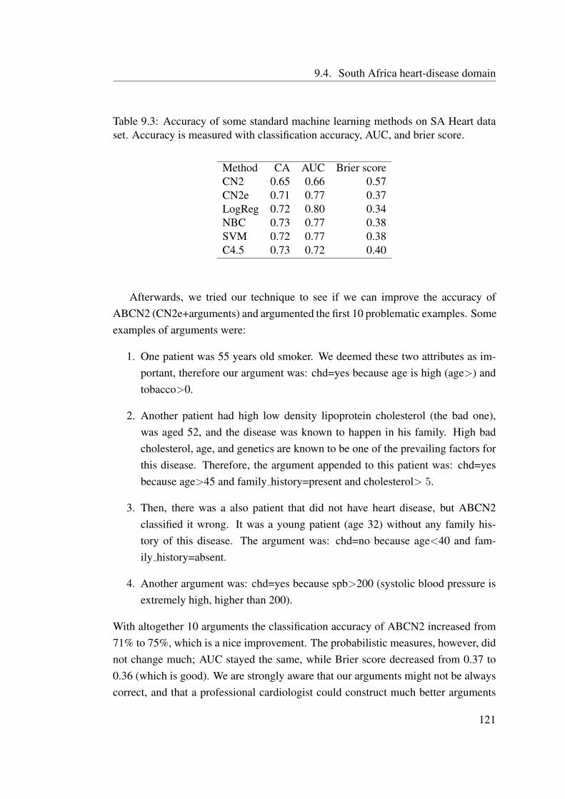
9.4. South Africa heart-disease domain
Table 9.3: Accuracy of some standard machine learning methods on SA Heart dataset. Accuracy is measured with classification accuracy, AUC, and brier score.
Method CA AUC Brier scoreCN2 0.65 0.66 0.57CN2e 0.71 0.77 0.37LogReg 0.72 0.80 0.34NBC 0.73 0.77 0.38SVM 0.72 0.77 0.38C4.5 0.73 0.72 0.40
Afterwards, we tried our technique to see if we can improve the accuracy ofABCN2 (CN2e+arguments) and argumented the first 10 problematic examples. Someexamples of arguments were:
1. One patient was 55 years old smoker. We deemed these two attributes as im-portant, therefore our argument was: chd=yes because age is high (age>) andtobacco>0.
2. Another patient had high low density lipoprotein cholesterol (the bad one),was aged 52, and the disease was known to happen in his family. High badcholesterol, age, and genetics are known to be one of the prevailing factors forthis disease. Therefore, the argument appended to this patient was: chd=yesbecause age>45 and family history=present and cholesterol> 5.
3. Then, there was a also patient that did not have heart disease, but ABCN2classified it wrong. It was a young patient (age 32) without any family his-tory of this disease. The argument was: chd=no because age<40 and fam-ily history=absent.
4. Another argument was: chd=yes because spb>200 (systolic blood pressure isextremely high, higher than 200).
With altogether 10 arguments the classification accuracy of ABCN2 increased from71% to 75%, which is a nice improvement. The probabilistic measures, however, didnot change much; AUC stayed the same, while Brier score decreased from 0.37 to0.36 (which is good). We are strongly aware that our arguments might not be alwayscorrect, and that a professional cardiologist could construct much better arguments
121

9. INTRODUCTORY EXPERIMENTS
for problematic examples. However, the idea of this experiment was to show howsuch, imperfect arguments can still improve the quality of induced hypothesis.
At this point of the experiment, we wondered if it would be possible to combinehigh classification accuracy of ABCN2 with good probability prediction of logisticregression. We tried to use the ability of PILAR’s classification (see chapter 7) toimprove other methods using rules, in this case the logistic regression. Initially, wecombined logistic regression with CN2e (without arguments) and got exactly the re-sults of logistic regression - rules did not contribute at all. Alternatively, we triedto use arguments to improve logistic regression with PILAR. Starting with argu-menting first 10 problematic cases did not practically change the accuracy of logisticregression. Even, after 20 arguments, the accuracy was almost still unchanged: clas-sification accuracy increased to 0.73, AUC increases to 0.81, while the Brier scoreincreased to 0.35. We were unable to improve logistic regression without knowledgeof the domain.
However, the last part of this experiment is not necessarily only a negative re-sult. It should be noted that, while the accuracy of the hypothesis stayed the same,its structure changed a lot to reflect the arguments that were provided to examples.This could be useful especially in medicine, where experts often prefer models thatcorrespond to their knowledge, even if they are less accurate. For example, in one ofour past applications (not related to argument based machine learning) [ADZ+07],the main medical expert Noriaki Aoki clearly preferred the model induced by naiveBayesian classifier to the one induced by logistic regression, although logistic regres-sion was significantly better, since he could better understand the former one.
122

Chapter 10
Arguments Implying New Attributes
An argument in rule learning was defined as a conclusion and a conjunction of rea-sons, where each reason mentions some property of the example. Initially, the prop-erty of the example corresponded to its attribute value, however in some of our ex-periments this interpretation was not sufficient. It can happen in two possible cases:
• A reason is a combination of several attributes, where combination is not aconjunction of these attributes. In these cases, we will construct a new attributefrom the already existent and add it to the domain.
• A reason can mention a property that is not yet described with the currentattribute set. In such cases, we need to add a new attribute to the domain andobtain values of the new attribute for all learning examples.
10.1 Japanese credit screening database
Japanese Credit Screening Database contains 125 persons applying for credit de-scribed with 10 attributes. The class attribute is whether a person did get the credit ornot. This domain definition also contains imperfect prior knowledge (accuracy 83%on the examples) - it was generated by talking to individuals at a Japanese companythat grants credit. This prior knowledge will be used in our experiment as a substi-tute for the domain expert. We will assume that this ”expert” cannot give a completedefinition of the target concept, but can only give arguments for certain examples.Again, data was split to a learn set (70%) and test set (30%).
123
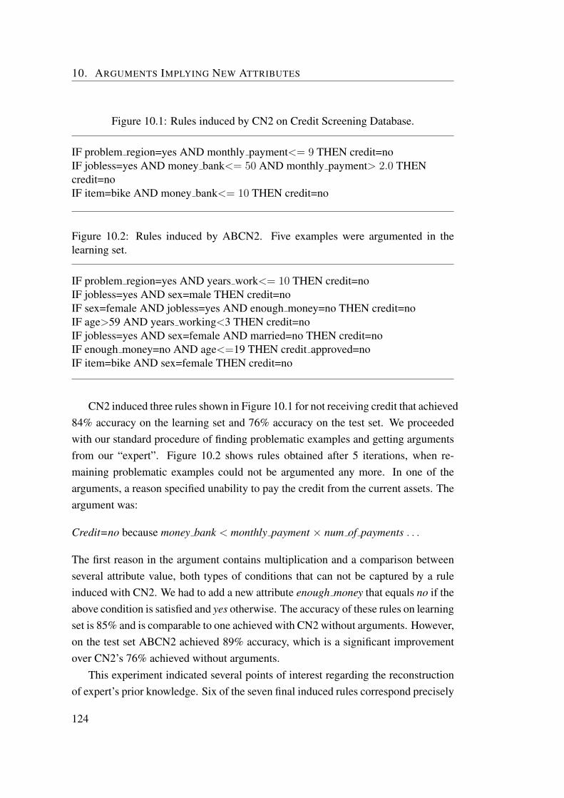
10. ARGUMENTS IMPLYING NEW ATTRIBUTES
Figure 10.1: Rules induced by CN2 on Credit Screening Database.
IF problem region=yes AND monthly payment<= 9 THEN credit=noIF jobless=yes AND money bank<= 50 AND monthly payment> 2.0 THENcredit=noIF item=bike AND money bank<= 10 THEN credit=no
Figure 10.2: Rules induced by ABCN2. Five examples were argumented in thelearning set.
IF problem region=yes AND years work<= 10 THEN credit=noIF jobless=yes AND sex=male THEN credit=noIF sex=female AND jobless=yes AND enough money=no THEN credit=noIF age>59 AND years working<3 THEN credit=noIF jobless=yes AND sex=female AND married=no THEN credit=noIF enough money=no AND age<=19 THEN credit approved=noIF item=bike AND sex=female THEN credit=no
CN2 induced three rules shown in Figure 10.1 for not receiving credit that achieved84% accuracy on the learning set and 76% accuracy on the test set. We proceededwith our standard procedure of finding problematic examples and getting argumentsfrom our “expert”. Figure 10.2 shows rules obtained after 5 iterations, when re-maining problematic examples could not be argumented any more. In one of thearguments, a reason specified unability to pay the credit from the current assets. Theargument was:
Credit=no because money bank < monthly payment × num of payments . . .
The first reason in the argument contains multiplication and a comparison betweenseveral attribute value, both types of conditions that can not be captured by a ruleinduced with CN2. We had to add a new attribute enough money that equals no if theabove condition is satisfied and yes otherwise. The accuracy of these rules on learningset is 85% and is comparable to one achieved with CN2 without arguments. However,on the test set ABCN2 achieved 89% accuracy, which is a significant improvementover CN2’s 76% achieved without arguments.
This experiment indicated several points of interest regarding the reconstructionof expert’s prior knowledge. Six of the seven final induced rules correspond precisely
124
10.2. ZEUS credit assignment problem
to complete background knowledge given by experts. This was achieved by askingour “expert” to explain only five examples, which indicates the effectiveness of theABML refinement loop. This also indicates how effective ABML is as a tool forextracting expert’s informal background knowledge. Imagine that we did not haveexperts’ prior knowledge already formalized, and that we wanted to extract it from theexpert. The way to do this with interactive use of ABCN2, is to generate questionsfor the expert by identifying critical examples. Expert’s explanations in terms ofarguments of the five critical cases would, in our example, be sufficient to completelyformalize the expert’s prior intuitions.
This experiment also nicely illustrates the difference between induced rules re-sulting from data only, and actual causal rules that generated the data. Both hypothe-ses, with and without arguments, have a similar accuracy on the learning set, but toa domain expert the first set of rules would be difficult to understand as they showunfamiliar dependencies. Moreover, the first set of rules scored significantly loweraccuracy on the test set, meaning that the first hypothesis merely reflected a spuriousrelation in the learning set.
10.2 ZEUS credit assignment problem
A similar learning problem to the one above - learning about credit status - occurredwithin European the 6th framework project ASPIC∗. Learning about credit status is apart of a larger business-to-business scenario used in ASPIC as the main large-scaledemonstration application for argument-based methods. In that experiment we alsoshowed how ABCN2 can be used to improve existing knowledge bases in argumen-tation based expert systems.
The main problem of the scenario is to determine whether client should be grantedcredit for a purchase. This is determined by the system through a set of if-thenbusiness rules. A part of them is used to determine whether the applicant creditstatus is “good”, “bad”, “average”, or “unavailable”. In the initial knowledge base(given by experts), the following three rules were used for classification:
Credit History = Good If all past debts were paid before or on the date due.
Credit History = Average If equal or less number of past debts were paid in lessthan a week late, to the ones paid on time.
∗Argument Service Platform with Integrated Components (ASPIC),http://www.argumentation.org/
125
10. ARGUMENTS IMPLYING NEW ATTRIBUTES
Credit History = Bad If more debts paid after the deadline than the ones paid ontime.
Along to classification rules, ZEUS also provided a data set of 5000 companiesdescribed with 18 attributes (four of them actually relevant for credit history). Webegan the experiment with the induction of rules from 2500 examples (learning set)without considering given classification rules. The system learned a set of 40 rules.As there was a lot of data available, the method was able to correctly classify 95% ofexamples in test set (the remaining 2500 examples) which is a quite good result withrespect to classification accuracy.
In the next step we ran the algorithm for finding problematic example. It was acompany that had “bad” credit status as a class value. We looked up the values of thisexample and noticed that third rule from experts apply. This company did historicallypay more often late than on time (attributes past debts after date, past debts on time,past debts before time). The argument for bad is thus:
Credit History = Bad because past debts after date >> past debts on time + past debts before time
The problem with given argument that it is not consistent with the format of if-then rules learned by CN2. The condition part of a rule is a conjunction of severalattribute-value pairs, whereas our condition contains comparison of three attributevalues and also a sum of two of them. We solved this problem by constructing an-other boolean attribute that has value 1 when the above condition is true and 0 whenit is not. We named it “latePayer” and the argument thus changed to:
Credit History = Bad because latePayer = 1
With the additional argument and the same 2500 learning examples, ABCN2learned only 27 rules. Due to the argument and the new attribute the number of rulesfor classes “bad” and “average” dropped significantly. At the same time classificationaccuracy measured on test data was slightly improved to 97%.
In the next pass we repeated the search for problematic example, this time it wasfrom class “Credit history”=“good”. The argument from initial knowledge base wastherefore:
Credit History = Good because past debts after date < 1
126
10.3. Construction of sophisticated chess concepts
We relearned rules from learn set and the two given arguments and ABCN2 in-duced only six rules, while classification accuracy of these rules on test set increasedto 99.9%. This is a significant improvement in terms of classification accuracy, buteven more spectacular is the improvement in terms of the complexity of the inducedtheories, from the initial 40 rules to 6 only. The improvement after the first argumentis expectable, as CN2 is incapable to learning a rule of that format. However, theimprovement after the second argument is surprising, as there should be no reasonwhy a rule learner could not find this condition automatically. The problem is themyopical property of rule learning evaluation functions. These add one condition ata time, however the debts after date < 1 by itself does not increase the probabilityof class good. The condition becomes good only after adding another condition.
10.3 Construction of sophisticated chess concepts
In this case study, we demonstrate the use of argument based machine learning forknowledge acquisition of a sophisticated chess concept [MGK+08]. Knowledge ac-quisition is still one of the most difficult tasks of artificial intelligence [Fei84]. Theproblem was addressed in various ways [Boo89; Chk03; Coo94], proposing assortedcognitive techniques like interviews, observations, analogy, etc. to elicit as muchknowledge from experts as possible. Nevertheless, the problem still remains largelyunsolved [Fei03]. Machine learning has long ago been proposed as an alternative wayof addressing this problem [FR86; For86]. While it was shown that it can be success-ful in building knowledge bases [LS95], the major problem with this approach is thatautomatically induced models rarely conform to the way an expert wants the knowl-edge organised and expressed. Models that are incomprehensible have less chance tobe trusted by experts and users alike. In striving for better accuracy, modern trends inmachine learning (e.g. support vector machines) do not seem to be doing anything toalleviate this problem. A common view is that a combination of a domain expert andmachine learning would yield the best results [WWZ99]. And this is where ABMLcomes into place.
For the particular chess concept, we considered the elicitation of the well-knownchess concept of bad bishop. This concept is used in a chess tutoring applicationdeveloped by Sadikov et al. [SMG+06]. The idea is to improve the chess playingprograms with an understanding of static positions. While todays chess playing pro-grams are extremely good at playing chess, their use for commenting or tutoring is
127
10. ARGUMENTS IMPLYING NEW ATTRIBUTES
rather limited. Such programs evaluate chess positions numerically, but are then notable to explain a numerical evaluation in terms of concepts that human chess playersuse when they reason about the position. For example, the program may say thatthe current positions value is 1.70 in favor of White. Now the beginner chess playerwould ask “Why”? An answer, which is beyond today’s chess programs, might be:“Because Black has a bad bishop.”
10.3.1 Experiment
Watson [Wat99] gives the following definition of a bad bishop as traditional: a bishopthat is on the same colour of squares as its own pawns is bad, since its mobility isrestricted by its own pawns and it does not defend the squares in front of these pawns.Moreover, he puts forward that centralisation of these pawns is the main factor indeciding whether the bishop is bad or not.
In the experiments, the dataset for learning consisted of 200 middlegame posi-tions from real chess games where the black player has only one bishop†. Thesebishops were then a subject of evaluation by the experts‡. In 78 cases, the bishopswere assessed as bad. Each position had also been statically evaluated (i.e. withoutapplying any search) by the evaluation function of the well-known open source chessprogram CRAFTY, and its positional feature values§ served as attribute values forlearning. We randomly selected 100 positions for learning and 100 for testing (strat-ification was used, preserving the proportion of positive and negative examples).
In the first iteration of the previously mentioned process, only CRAFTY’s posi-tional features were used and no arguments have been given yet. ABCN2 inducedall together 4 rules achieving 72% classification accuracy on the test set. Figure 10.3shows the first critical example, automatically selected by our algorithm.
The initial rules failed to classify this example as “not bad”, as was previouslyjudged by the experts. The following question was given to the experts: “Why isthe black bishop not bad?” It turned out that the concept mentioned by the experts(see the caption in Figure 10.3) was not yet present in the domain attributes - theonly CRAFTY’s positional feature that could potentially describe bishop’s mobility,BLACK BISHOPS MOBILITY, expresses the number of squares that the bishop at-
†The learning data set and a detailed explanation of domain’s attributes can be found at:http://www.ailab.si/matej/.
‡The chess expertise was provided by woman grandmaster Jana Krivec and FIDE master MatejGuid.
§CRAFTY’s evaluation function uses about 100 positional features.
128

10.3. Construction of sophisticated chess concepts
Figure 10.3: Why is the black bishop not bad? The experts used their domain knowl-edge to produce the following answer: “The black bishop is not bad, since its mobilityis not seriously restricted by the pawns of both players.”
tacks, but doing so takes into account all pieces (not only pawns) that block thebishop’s diagonals, restricting its mobility. A new attribute,IMPROVED BISHOP MOBILITY, was therefore programmed and included into thedomain. It is the number of squares accessible to the bishop, taking into account onlyown and opponent’s pawn structure. Based on the experts’ explanation, the argument“IMPROVED BISHOP MOBILITY is high” was added to this example.
Taking only the bishop’s mobility into account turned out not to be enough forABCN2 to determine the goodness of the bishop. Also, the method, which at thetime only had CRAFTY’s attributes and the newly included attribute at its disposal,failed to find additional restrictions to improve the experts’ argument. To solve thisproblem, we used the idea of counter examples presented in Chapter 8. The methodfound a counter example shown in Figure 10.4. This example is classified as “bad”,although the value of the attribute IMPROVED BISHOP MOBILITY is high.
The experts were now asked to compare the black bishops in the two examples:“Why is the black bishop in Figure 10.4 bad, and the bishop in Figure 10.3 is not?”Again, the experts have been asked to give a description based on their knowledge inthe presented domain. Based on this description (given in Figure 10.4), another at-tribute, BAD PAWNS, was included into the domain. This attribute evaluates pawnsthat are on the colour of the square of the bishop (“bad” pawns in this sense). Withsome help of the experts, a look-up table with predefined values for the pawns that areon the same colour of squares as the bishop was designed in order to assign weightsto such pawns. According to the previously mentioned Watson’s definition, central-isation of the pawns was taken into account. The argument given to the exampleshown in Figure 10.3 was then extended to “IMPROVED BISHOP MOBILITY is
129
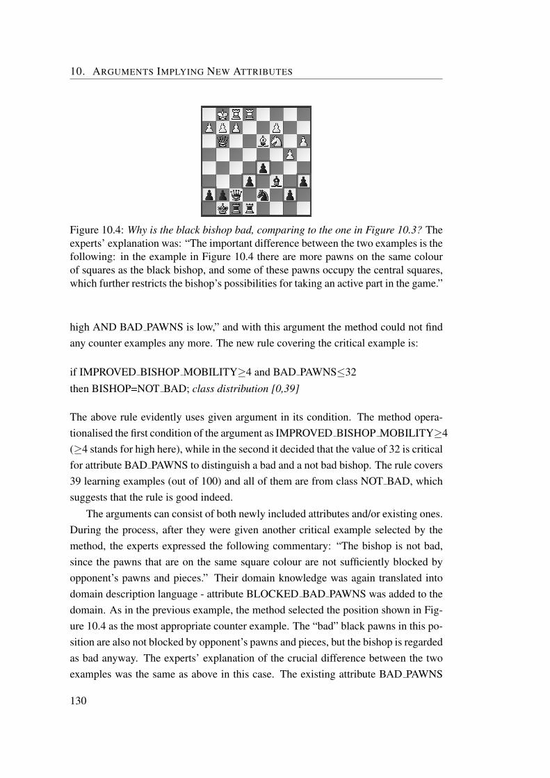
10. ARGUMENTS IMPLYING NEW ATTRIBUTES
Figure 10.4: Why is the black bishop bad, comparing to the one in Figure 10.3? Theexperts’ explanation was: “The important difference between the two examples is thefollowing: in the example in Figure 10.4 there are more pawns on the same colourof squares as the black bishop, and some of these pawns occupy the central squares,which further restricts the bishop’s possibilities for taking an active part in the game.”
high AND BAD PAWNS is low,” and with this argument the method could not findany counter examples any more. The new rule covering the critical example is:
if IMPROVED BISHOP MOBILITY≥4 and BAD PAWNS≤32then BISHOP=NOT BAD; class distribution [0,39]
The above rule evidently uses given argument in its condition. The method opera-tionalised the first condition of the argument as IMPROVED BISHOP MOBILITY≥4(≥4 stands for high here), while in the second it decided that the value of 32 is criticalfor attribute BAD PAWNS to distinguish a bad and a not bad bishop. The rule covers39 learning examples (out of 100) and all of them are from class NOT BAD, whichsuggests that the rule is good indeed.
The arguments can consist of both newly included attributes and/or existing ones.During the process, after they were given another critical example selected by themethod, the experts expressed the following commentary: “The bishop is not bad,since the pawns that are on the same square colour are not sufficiently blocked byopponent’s pawns and pieces.” Their domain knowledge was again translated intodomain description language - attribute BLOCKED BAD PAWNS was added to thedomain. As in the previous example, the method selected the position shown in Fig-ure 10.4 as the most appropriate counter example. The “bad” black pawns in this po-sition are also not blocked by opponent’s pawns and pieces, but the bishop is regardedas bad anyway. The experts’ explanation of the crucial difference between the twoexamples was the same as above in this case. The existing attribute BAD PAWNS
130
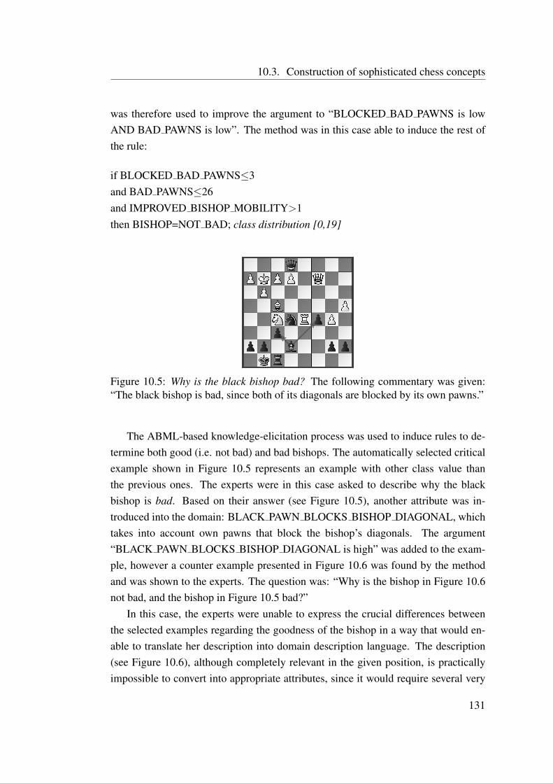
10.3. Construction of sophisticated chess concepts
was therefore used to improve the argument to “BLOCKED BAD PAWNS is lowAND BAD PAWNS is low”. The method was in this case able to induce the rest ofthe rule:
if BLOCKED BAD PAWNS≤3and BAD PAWNS≤26and IMPROVED BISHOP MOBILITY>1then BISHOP=NOT BAD; class distribution [0,19]
Figure 10.5: Why is the black bishop bad? The following commentary was given:“The black bishop is bad, since both of its diagonals are blocked by its own pawns.”
The ABML-based knowledge-elicitation process was used to induce rules to de-termine both good (i.e. not bad) and bad bishops. The automatically selected criticalexample shown in Figure 10.5 represents an example with other class value thanthe previous ones. The experts were in this case asked to describe why the blackbishop is bad. Based on their answer (see Figure 10.5), another attribute was in-troduced into the domain: BLACK PAWN BLOCKS BISHOP DIAGONAL, whichtakes into account own pawns that block the bishop’s diagonals. The argument“BLACK PAWN BLOCKS BISHOP DIAGONAL is high” was added to the exam-ple, however a counter example presented in Figure 10.6 was found by the methodand was shown to the experts. The question was: “Why is the bishop in Figure 10.6not bad, and the bishop in Figure 10.5 bad?”
In this case, the experts were unable to express the crucial differences betweenthe selected examples regarding the goodness of the bishop in a way that would en-able to translate her description into domain description language. The description(see Figure 10.6), although completely relevant in the given position, is practicallyimpossible to convert into appropriate attributes, since it would require several very
131
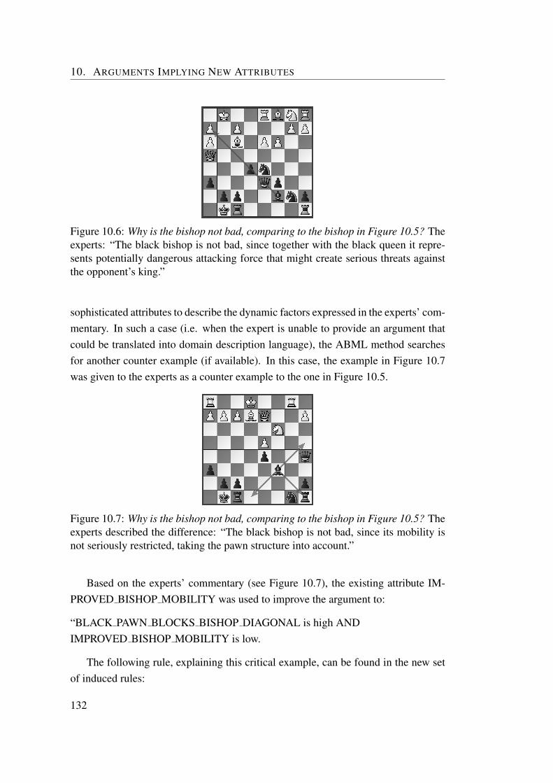
10. ARGUMENTS IMPLYING NEW ATTRIBUTES
Figure 10.6: Why is the bishop not bad, comparing to the bishop in Figure 10.5? Theexperts: “The black bishop is not bad, since together with the black queen it repre-sents potentially dangerous attacking force that might create serious threats againstthe opponent’s king.”
sophisticated attributes to describe the dynamic factors expressed in the experts’ com-mentary. In such a case (i.e. when the expert is unable to provide an argument thatcould be translated into domain description language), the ABML method searchesfor another counter example (if available). In this case, the example in Figure 10.7was given to the experts as a counter example to the one in Figure 10.5.
Figure 10.7: Why is the bishop not bad, comparing to the bishop in Figure 10.5? Theexperts described the difference: “The black bishop is not bad, since its mobility isnot seriously restricted, taking the pawn structure into account.”
Based on the experts’ commentary (see Figure 10.7), the existing attribute IM-PROVED BISHOP MOBILITY was used to improve the argument to:
“BLACK PAWN BLOCKS BISHOP DIAGONAL is high ANDIMPROVED BISHOP MOBILITY is low.
The following rule, explaining this critical example, can be found in the new setof induced rules:
132

10.3. Construction of sophisticated chess concepts
0 1 2 3 4 5 6 7 8
Iterations
0.7
0.8
0.9
1.0
CA
.............................................................................................................................................................................................................
................................................................................................................................................................................................................................................................................................................................
......................................
....................
∗∗∗∗∗∗∗∗ ∗ ∗ ∗ ∗ ∗ ∗ ∗ ∗ ∗ ∗ ∗ ∗ ∗ ∗ ∗ ∗
.............................................................................. ............. ............. .............
............. ............. ............. ............. ............. ............. ............. ............. ............. ............. ............. ............. .............
.........................
.............................................
Figure 10.8: Progress of classification accuracies (CA) through iterations for ABCN2(solid line), logistic regression (stars ∗), C4.5 (dashed line) and classic CN2 (dots).
if BLACK PAWN BLOCKS BISHOP DIAGONAL≥20and IMPROVED BISHOP MOBILITY≤3then BISHOP=BAD; class distribution [18,0]
In total, there were eight critical examples presented to the experts The finalmodel scored 95% accuracy on the test set.
10.3.2 Discussion
The ABML-based knowledge-elicitation process presented in our case study con-sisted of eight (8) iterations. During the process, seven (7) arguments were attachedto automatically selected critical examples, and five (5) new attributes were sug-gested by arguments and therefore included into the domain. This experiment alsodemonstrated the use of counter-examples; in some of the iterations, initially givenarguments were not enough for ABCN2 to induce a good rule, therefore experts hadto revise their arguments using counter-examples. After each iteration, the obtainedrules were evaluated on the test dataset. The improvement of the model is evident:from the initial 72% classification accuracy (Brier score 0.39, AUC 0.80), the final95% accuracy (Brier score 0.11, AUC 0.97) was achieved after the end of the process.
The question is, whether these improvements were mainly due to the addition ofnew attributes or were the arguments also just important? The Figure 10.8 shows thatthe arguments also mattered significantly. We compared the progressions of clas-
133

10. ARGUMENTS IMPLYING NEW ATTRIBUTES
sification accuracies of ABCN2 with some other (“non-ABML” - using only newlyadded attributes) machine learning algorithms, namely logistic regression, decisiontrees (C4.5), and the classic CN2. The accuracies of all methods improved during theprocess, however ABCN2 (which also used the arguments given by the experts) out-performed all the others. The obtained results suggest that the performance of otheralgorithms could also be improved by adding appropriate new attributes. However,using arguments is likely to lead to even more accurate models.
The main advantage of ABML over classical machine learning is the ability totake advantage of expert’s prior knowledge in the induction procedure. This leadsto hypotheses comprehensible to experts, as it explains learning examples using thesame arguments as the expert did. In our case study this was confirmed by chessexperts. According to them, the final set of rules are more alike to their understandingof the bad bishop concept than the initial rules were. Furthermore, the final rules werealso recognised to be in accordance with the traditional definition of a bad bishop.
Our domain experts clearly preferred the ABML approach to manual knowledgeacquisition. The formalisation of the concept of bad bishop turned out to be beyondthe practical ability of our chess experts (a master and a woman grandmaster). Aftertrying to manual define this concept, their rules achieved 56% accuracy on the testset. They described the process as time consuming and hard, mainly because it isdifficult to consider all relevant elements. ABML facilitates knowledge acquisitionby fighting these problems directly. Experts do not need to consider all possibly rel-evant elements, but only elements relevant for a specific case, which is much easier.Moreover, by selecting only critical examples, the time of experts involvement isdecreased, making the whole process much less time consuming.
134

Chapter 11
Automatically Extracted Argumentsfrom Text
In ABML applications, arguments are usually provided by domain experts. In thischapter, we will demonstrate a possible way of extracting arguments from text andusing them in ABML. The work was done as a part of the X-Media∗ project, which isan European project that addresses the issue of cross-media knowledge managementin complex distributed environments.
11.1 Extracting arguments from text
The extraction of arguments from text is based on relation extraction from text. Rela-tion extraction is an important task in natural language processing, with many prac-tical applications such as question answering, ontology population, and informationretrieval. It requires the analysis of textual documents, with the aim of recogniz-ing particular types of relations between named entities, nominals, and pronouns.Reliably extracting relations in natural-language documents is still a laborious andunsolved problem. Traditionally, relation extraction systems have been trained torecognize relations between names of people, organizations, locations, and proteins.In the last two decades, several evaluation campaigns such as MUC [MUC], ACE[ACE], SemEval [sem] have helped to understand and properly formalize the prob-lem, and provide comparative benchmarks.
We are interested in finding semantic relations between class values and descrip-tive attributes (taken from data), and using them as arguments. For example, taking
∗http://www.x-media-project.org/
135

11. AUTOMATICALLY EXTRACTED ARGUMENTS FROM TEXT
the ZOO domain from Chapter 8, given the class value reptile and the attribute eggswe are interested in relations such as “Most reptiles lay eggs” and “Reptiles hatcheggs.” Specifically, the relationships that exist between classes and attributes are ex-tracted from the whole English Wikipedia,† an online encyclopedia written collabo-ratively by volunteers, that has grown to become one of the largest online repositoriesof encyclopedic knowledge, with millions of articles available for a large number oflanguages.
To extract such relations from textual documents, we have to deal with two majorproblems. The first concerns the lack of information on the relation type we areseeking. In relation extraction, we usually know in advance the type of the relationsto be extracted, here we only know class values and attributes, namely the conclusionand reasons of a possible relation. Thus, the task is restricted to discover whether ornot a relation exists between class and an attribute.
The second problem is related with the lexicalization of the class values and at-tribute descriptions. The names of attributes and classes should be meaningful, or,in other words, should be similar to those used in texts. Using their backgroundknowledge, humans can naturally interpret the concepts expressed by class valuesand attributes, however, due to the variability of natural language, it can be verydifficult to find occurrences of the lexicalizations of such concepts in the same sen-tence and, consequently, to determine whether or not a relation exists. To address thefirst problem, we do not try to find specific assertions of relations in text, but ratherwe exploit the simple idea that if many different sentences reference both the classvalue and attribute, then the class value and attribute are likely to be related. On theother hand, to deal with the variability of natural language, we generated alterna-tive lexical variants using a WordNet [Fel98], a lexical database containing semanticrelations among words. Specifically, we generated variants for all class values and at-tributes using the following semantic relations in WordNet: synonyms (e.g., breathe→ respire) and morphological derivations (e.g., predator→ predators).
As most relation extraction systems [HSG04; BM05; GLR07], we identify rela-tions mentioned in text documents considering only those pairs that are mentionedin the same sentence. Let c1, . . . , ck be class values in data and a1, . . . , an attributes.Then, the number of relations #r(ci, aj) is defined as the number of sentences acrossthe whole English Wikipedia, where the class ci and the attribute aj co-occur.
We shall now define the construction of an argument given the number of relations
†http://en.wikipedia.org
136
11.2. Case study: animal classification
between class and attribute values. An argument is a conjunction of a set of reasons,where each reason is related to a single attribute in the domain. To determine whetherand attribute aj is a possible reason for class ci, we first evaluate whether #r(ci, aj)is statistically different from the expected value E(#r(ci, aj)), namely if the numbercould be obtained purely by chance. A possible method for this task is the standardχ2 test for 2× 2 matrices.
When #r(ci, aj) is statistically different from E(#r(ci, aj)), it can be eitherhigher or lower. If #r(ci, aj) > E(#r(ci, aj)), then we say that aj is a positivereason for ci. Such a positive argument can be given to an example if it is from classci and the value of aj is “positive”. The positiveness of attribute values must be de-fined prior to learning and it intends to distinguish between values that should occurmore frequently in the class-attribute relations in text than it is expected. Although,it is impossible to say which of the values will have this property, we believe thata good heuristics to select positive attribute values is to select those that ascribe thepresence of a property described by aj to the example. For instance, if an animal hasthe value of attribute breathes 1, this value states that the animal is breathing (pres-ence of this property), and the value of attribute is positive. If the number of foundrelations is less than expected, i.e. #r(ci, aj) < E(#r(ci, aj)), then we can use suchreason only if the example has negative value of aj .
An argument for a certain example is thus constructed from all positive and nega-tive reasons consistent with the values of this example. Sometimes, such an argumentwill be overly specific. To alleviate this problem all arguments are pruned with REP(reduced error pruning) [Fur97] principle before they are appended to the example.
11.2 Case study: animal classification
The approach will be illustrated and evaluated on the domain ZOO, the same one asused in the first section of Chapter 8. We began the experiment by learning rules withABCN2 without any arguments extracted from text. Learning and testing on the fulldata set accounted for 100% classification accuracy. Induced rules were:
• IF milk=yes THEN type=mammal
• IF feathers=yes THEN type=bird
• IF eggs=yes AND fins=yes THEN type=fish
137
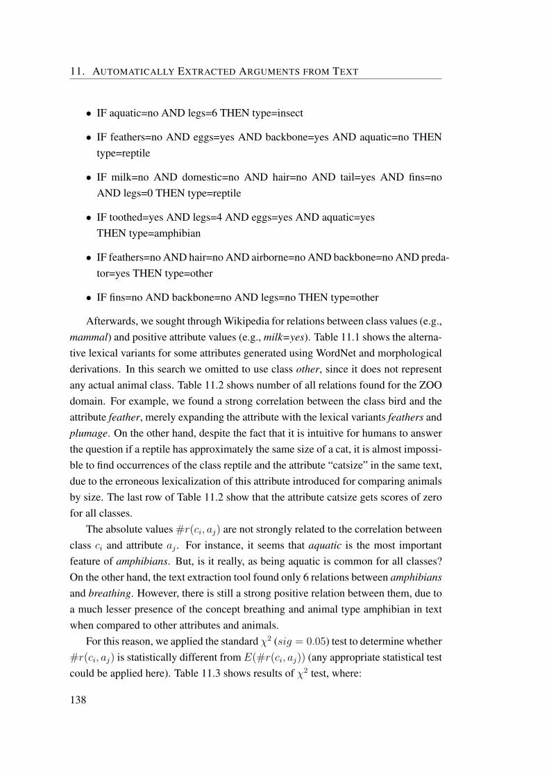
11. AUTOMATICALLY EXTRACTED ARGUMENTS FROM TEXT
• IF aquatic=no AND legs=6 THEN type=insect
• IF feathers=no AND eggs=yes AND backbone=yes AND aquatic=no THENtype=reptile
• IF milk=no AND domestic=no AND hair=no AND tail=yes AND fins=noAND legs=0 THEN type=reptile
• IF toothed=yes AND legs=4 AND eggs=yes AND aquatic=yesTHEN type=amphibian
• IF feathers=no AND hair=no AND airborne=no AND backbone=no AND preda-tor=yes THEN type=other
• IF fins=no AND backbone=no AND legs=no THEN type=other
Afterwards, we sought through Wikipedia for relations between class values (e.g.,mammal) and positive attribute values (e.g., milk=yes). Table 11.1 shows the alterna-tive lexical variants for some attributes generated using WordNet and morphologicalderivations. In this search we omitted to use class other, since it does not representany actual animal class. Table 11.2 shows number of all relations found for the ZOOdomain. For example, we found a strong correlation between the class bird and theattribute feather, merely expanding the attribute with the lexical variants feathers andplumage. On the other hand, despite the fact that it is intuitive for humans to answerthe question if a reptile has approximately the same size of a cat, it is almost impossi-ble to find occurrences of the class reptile and the attribute “catsize” in the same text,due to the erroneous lexicalization of this attribute introduced for comparing animalsby size. The last row of Table 11.2 show that the attribute catsize gets scores of zerofor all classes.
The absolute values #r(ci, aj) are not strongly related to the correlation betweenclass ci and attribute aj . For instance, it seems that aquatic is the most importantfeature of amphibians. But, is it really, as being aquatic is common for all classes?On the other hand, the text extraction tool found only 6 relations between amphibiansand breathing. However, there is still a strong positive relation between them, due toa much lesser presence of the concept breathing and animal type amphibian in textwhen compared to other attributes and animals.
For this reason, we applied the standard χ2 (sig = 0.05) test to determine whether#r(ci, aj) is statistically different from E(#r(ci, aj)) (any appropriate statistical testcould be applied here). Table 11.3 shows results of χ2 test, where:
138

11.2. Case study: animal classification
Table 11.1: The alternative lexical variants for attributes generated using WordNetand morphological derivations.
attribute alternative lexical variantshair hairs, fur, fursfeather feathers, plumageegg eggs, spawn, spawnsmilk milkingairborne winged...domestic domesticated, petcatsize -
Table 11.2: Number of positive relations #r(ci, aj) between animal classes and at-tributes found in Wikipedia.
amphibian reptile insect mammal bird fishhair 1 16 70 187 106 87
feathers 0 14 17 15 894 31eggs 34 117 339 174 894 645milk 2 2 10 67 25 120
airborne 2 15 117 15 196 21aquatic 81 184 271 1008 284 1072
predator 5 16 123 95 285 217toothed 10 59 54 150 102 250
backbone 0 1 3 11 7 51breathes 6 3 8 11 16 45
venomous 6 43 39 44 41 47fins 4 4 3 17 21 529legs 27 42 206 51 364 111tail 16 26 53 57 504 279
domestic 9 40 31 81 317 166catsize 0 0 0 0 0 0
value 0 means that the relation is not significant;
value 1 denotes positive reasons, and
value -1 denotes negative reasons.
Table 11.3 shows which of the attributes can be used as arguments for every class.For example, in the case of amphibians, we can use attributes aquatic, breathes, andlegs as reasons in the argument, if the values of the corresponding case are positive
139
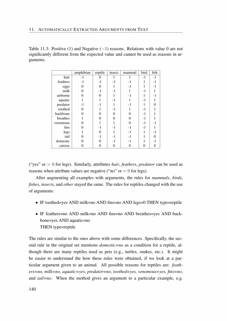
11. AUTOMATICALLY EXTRACTED ARGUMENTS FROM TEXT
Table 11.3: Positive (1) and Negative (−1) reasons. Relations with value 0 are notsignificantly different from the expected value and cannot be used as reasons in ar-guments.
amphibian reptile insect mammal bird fishhair -1 0 1 1 -1 -1
feathers -1 -1 -1 -1 1 -1eggs 0 0 1 -1 1 -1milk 0 -1 -1 1 -1 1
airborne 0 0 1 -1 1 -1aquatic 1 1 -1 1 -1 1
predator -1 -1 1 -1 1 0toothed 0 1 -1 1 -1 1
backbone 0 0 0 0 -1 1breathes 1 0 0 0 -1 1
venomous 0 1 1 0 -1 -1fins 0 -1 -1 -1 -1 1legs 1 0 1 -1 1 -1tail 0 -1 -1 -1 1 0
domestic 0 0 -1 -1 1 -1catsize 0 0 0 0 0 0
(“yes” or > 0 for legs). Similarly, attributes hair, feathers, predator can be used asreasons when attribute values are negative (“no” or = 0 for legs).
After augmenting all examples with arguments, the rules for mammals, birds,fishes, insects, and other stayed the same. The rules for reptiles changed with the useof arguments:
• IF toothed=yes AND milk=no AND fins=no AND legs=0 THEN type=reptile
• IF feathers=no AND milk=no AND fins=no AND breathes=yes AND back-bone=yes AND aquatic=noTHEN type=reptile
The rules are similar to the ones above with some differences. Specifically, the sec-ond rule in the original set mentions domestic=no as a condition for a reptile, al-though there are many reptiles used as pets (e.g., turtles, snakes, etc.). It mightbe easier to understand the how these rules were obtained, if we look at a par-ticular argument given to an animal. All possible reasons for reptiles are: feath-ers=no, milk=no, aquatic=yes, predator=no, toothed=yes, venomous=yes, fins=no,and tail=no. When the method gives an argument to a particular example, e.g.
140
11.2. Case study: animal classification
pitviper, it uses only reasons that are true for this example. In the case of pitviper, therelevant reasons would thus be: feathers=no, milk=no, toothed=yes, venomous=yes,and fins=no. The complete argument is:
Pitviper is a reptile, because feathers=no and milk=no and toothed=yes andvenomous=yes and fins=no.
Afterwards, to remove the unnecessary conditions, the reduced error pruning mech-anism is applied and the resulting argument is:
Pitviper is a reptile, because milk=no and toothed=yes and fins=no.
The first rule for reptiles used this arguments as the basis and added a conditionlegs=0 to finalise the induction of the rule.
The rule for amphibians changed to:
• IF legs=4 AND breathes=yes AND aquatic=yes AND hair=no THEN type=amphibian.
The original and the new rule are again very alike. In the latter attributes toothed andeggs were replaced with breathes and hair. From a point of an expert, the secondrule is better, since it is not entirely true that amphibians do not have teeth. Most am-phibian larvae have tiny teeth. Nevertheless, although most adult amphibians retaintheir teeth, teeth can be reduced in size or not present at all.
We evaluated the method with 10-times repeated 10-fold cross-validation to avoideffects of randomness of one split only. In each iteration, all examples in the learnset were argumented, then a model was built from these and evaluated on the testset. Using ABCN2 without arguments resulted in 94.51% classification accuracy,while ABCN2 with arguments scored, on average, 96.75% classification accuracy.As a comparison, some standard machine learning methods (as implemented in Or-ange [DZ04]) scored 90% (SVM), 92.57% (C4.5) and 92.6% (naıve Bayes). Thescores differ from those in Chapter 8, since another type of evaluation was used.
141


Chapter 12
Can Imperfect Arguments beDamaging?
It may well happen that the expert, when argumenting examples, will make mistakesand supply imperfect arguments. We now turn to the question, how critically ABCN2depends on the quality of arguments?
Theories learned by ABCN2 have to be consistent with the given arguments. Inthe case of imperfect arguments, this may be a problem, as the resulting theories willreflect these imperfections, and possibly have lower accuracy than learning withoutarguments at all. In this chapter, we will give an experimental evidence that, ingeneral, this problem is unlikely to cause much damage.
We start with the expectation that accuracy of theories learned from examplesand arguments given by experts is higher than accuracy of hypotheses learned fromexamples and random arguments. Experts, obviously, have better knowledge of thedomain than simple guessing, and so the given experts’ arguments will be betterthan random arguments. Consequently, the induced hypotheses will be, on average,more accurate. The effect will be detrimental only if the expert exploits his or herknowledge to maliciously hinder learning by intentionally giving extremely bad, falsearguments. In the following we will not consider such extremely unnatural situations,but investigate whether completely uninformative, random arguments will damagethe performance in comparison with no arguments at all.
We made an experiment, using 25 UCI data sets [AN07], comparing CN2 withABCN2 using 2, 5, 10, or 20 randomly argumented examples. Each argumentedexample can have up to five random positive arguments, and each argument canhave up to five random reasons.
143
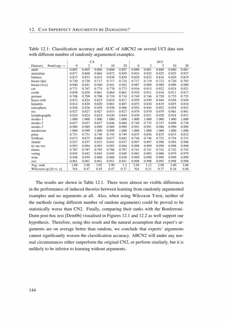
12. CAN IMPERFECT ARGUMENTS BE DAMAGING?
Table 12.1: Classification accuracy and AUC of ABCN2 on several UCI data setswith different number of randomly argumented examples.
CA AUCDataset↓ #rand.arg.→ 0 2 5 10 20 0 2 5 10 20adult 0.805 0.805 0.806 0.806 0.807 0.880 0.881 0.880 0.880 0.881australian 0.871 0.868 0.864 0.872 0.859 0.924 0.925 0.925 0.925 0.927balance 0.833 0.833 0.832 0.830 0.830 0.820 0.823 0.816 0.820 0.819breast (lju) 0.720 0.720 0.717 0.717 0.724 0.717 0.719 0.723 0.720 0.702breast (wsc) 0.940 0.941 0.940 0.941 0.942 0.987 0.989 0.989 0.989 0.990car 0.771 0.767 0.774 0.778 0.773 0.916 0.915 0.922 0.924 0.921credit 0.858 0.858 0.861 0.864 0.861 0.910 0.911 0.916 0.911 0.917german 0.708 0.709 0.708 0.710 0.710 0.749 0.746 0.750 0.755 0.755hayes-roth 0.832 0.824 0.825 0.810 0.817 0.959 0.959 0.944 0.958 0.949hepatitis 0.814 0.820 0.820 0.801 0.807 0.853 0.830 0.819 0.855 0.810ionosphere 0.926 0.926 0.929 0.920 0.906 0.954 0.954 0.952 0.954 0.952iris 0.927 0.927 0.927 0.933 0.927 0.979 0.979 0.979 0.981 0.981lymphography 0.824 0.824 0.824 0.830 0.844 0.930 0.931 0.928 0.924 0.931monks-1 1.000 1.000 1.000 1.000 1.000 1.000 1.000 1.000 1.000 1.000monks-2 0.657 0.657 0.657 0.646 0.666 0.740 0.735 0.747 0.699 0.738monks-3 0.989 0.989 0.989 0.989 0.989 0.991 0.991 0.988 0.990 0.989mushroom 1.000 0.999 1.000 0.999 1.000 1.000 1.000 1.000 1.000 1.000pima 0.751 0.751 0.749 0.745 0.749 0.835 0.836 0.835 0.833 0.832SAHeart 0.673 0.675 0.680 0.677 0.682 0.748 0.746 0.752 0.754 0.753shuttle 0.937 0.937 0.933 0.941 0.937 0.997 0.997 0.998 0.995 0.996tic-tac-toe 0.993 0.994 0.993 0.993 0.994 0.998 0.999 0.998 0.998 0.998titanic 0.787 0.787 0.785 0.786 0.787 0.741 0.741 0.742 0.742 0.742voting 0.945 0.942 0.945 0.945 0.949 0.983 0.983 0.986 0.979 0.979wine 0.948 0.959 0.960 0.960 0.938 0.999 0.999 0.999 0.999 0.999zoo 0.961 0.961 0.961 0.951 0.941 0.998 0.998 0.995 0.998 0.998Avg. rank 2.88 2.90 3.02 2.90 3.3 2.94 3.12 2.88 3.00 3.06Wilcoxon (p) [0 vs. x] NA 0.47 0.45 0.47 0.37 NA 0.31 0.37 0.34 0.48
The results are shown in Table 12.1. There were almost no visible differencesin the performance of induced theories between learning from randomly argumentedexamples and no arguments at all. Also, when using Wilcoxon T-test, neither ofthe methods (using different number of random arguments) could be proved to bestatistically worse than CN2. Finally, comparing their ranks with the Bonferroni-Dunn post-hoc test [Dem06] visualised in Figures 12.1 and 12.2 as well support ourhypothesis. Therefore, using this result and the natural assumption that expert’s ar-guments are on average better than random, we conclude that experts’ argumentscannot significantly worsen the classification accuracy. ABCN2 will under any nor-mal circumstances either outperform the original CN2, or perform similarly, but it isunlikely to be inferior to learning without arguments.
144
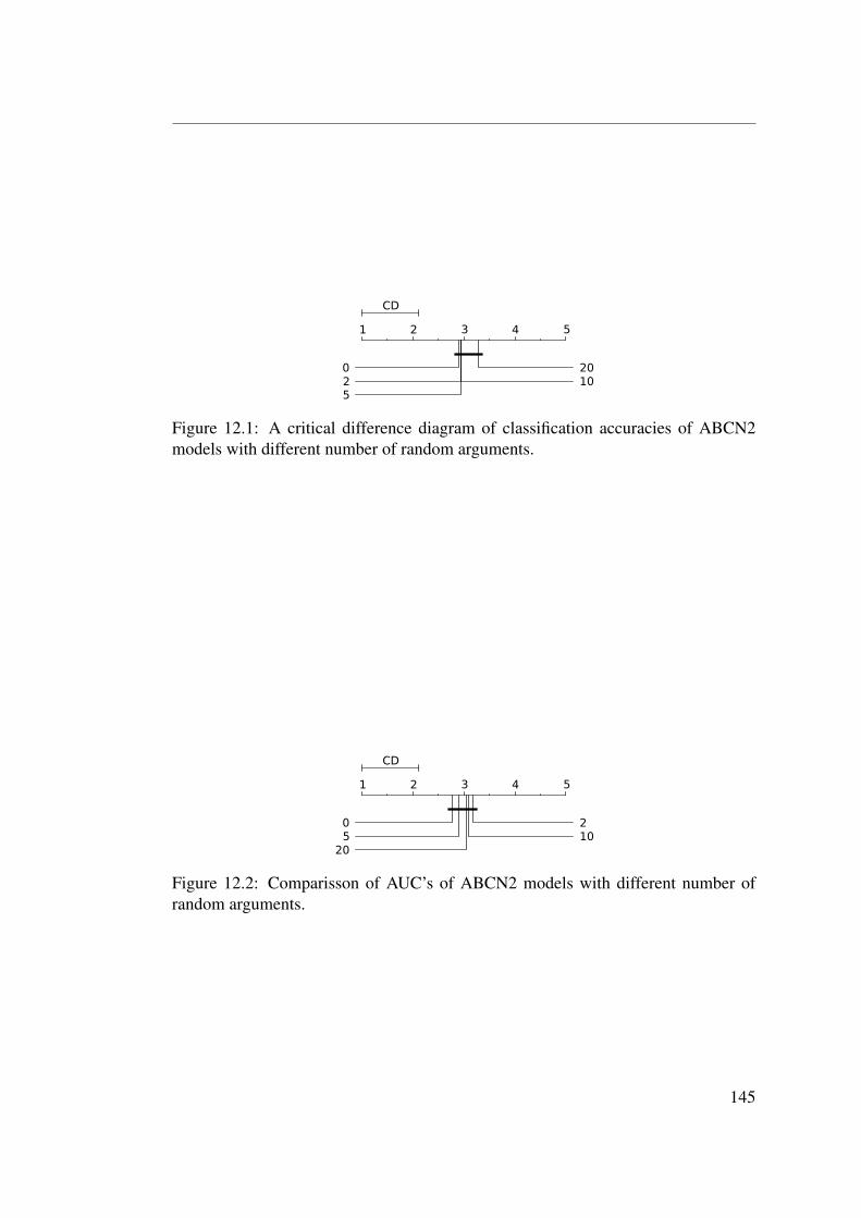
1 2 3 4 5
025
1020
CD
Figure 12.1: A critical difference diagram of classification accuracies of ABCN2models with different number of random arguments.
1 2 3 4 5
05
20102
CD
Figure 12.2: Comparisson of AUC’s of ABCN2 models with different number ofrandom arguments.
145


147

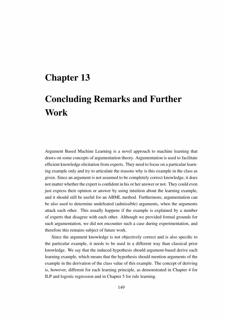
Chapter 13
Concluding Remarks and FurtherWork
Argument Based Machine Learning is a novel approach to machine learning thatdraws on some concepts of argumentation theory. Argumentation is used to facilitateefficient knowledge elicitation from experts. They need to focus on a particular learn-ing example only and try to articulate the reasons why is this example in the class asgiven. Since an argument is not assumed to be completely correct knowledge, it doesnot matter whether the expert is confident in his or her answer or not. They could evenjust express their opinion or answer by using intuition about the learning example,and it should still be useful for an ABML method. Furthermore, argumentation canbe also used to determine undefeated (admissible) arguments, when the argumentsattack each other. This usually happens if the example is explained by a numberof experts that disagree with each other. Although we provided formal grounds forsuch argumentation, we did not encounter such a case during experimentation, andtherefore this remains subject of future work.
Since the argument knowledge is not objectively correct and is also specific tothe particular example, it needs to be used in a different way than classical priorknowledge. We say that the induced hypothesis should argument-based derive eachlearning example, which means that the hypothesis should mention arguments of theexample in the derivation of the class value of this example. The concept of derivingis, however, different for each learning principle, as demonstrated in Chapter 4 forILP and logistic regression and in Chapter 5 for rule learning.
149

13. CONCLUDING REMARKS AND FURTHER WORK
In Chapter 5, we described the ABCN2 algortihm, an argument-based extensionof CN2, and argumented examples in rule learning. CN2 is a well-known methodfor learning rules, but very basic. The question is, if we would achieve even betterresults by using another, more sophisticated method, e.g. RIPPER [Coh95], whichuses reduced error pruning to post-prune induced rules? The only definite answerwould give an experiment, however, one needs to consider that CN2 as used in thisThesis is not the same CN2 as used a decade ago; the extreme value correction ofprobability estimates produces probability estimates that are closer to its true valuesand PILAR classification assigns each rule a weight of its importance - in a sense, itis a way to do what post-pruning does.
The PILAR classification technique described in Chapter 7 and extreme valuecorrection in probability estimates (Chapter 6) are both techniques that substantiallyimprove the quality of rule learning. However, they come at some computational cost.In extreme value correction, the required initial determination of the parameters ofthe extreme value distribution for the particular learning problem is typically roughlycomparable to the rest of rule learning in ABCN2. In PILAR, after rules have beeninduced, an optimisation to find the best parameters is needed. However, we do notregard the additional time required as a critical problem for ABCN2, since a largeportion of the time sink comes from interaction with experts, while time needed forlearning is negligible.
The argument based refinement loop iteratively selects critical examples thatshould be explained by an expert. In this way, experts need to focus on difficult casesonly and leave simple cases to the learning algorithm. At the moment, the algorithmalways suggests the most misclassified example as the most critical one. Althoughthis criterion is intuitive - ask what you do not know, and shows promising resultsin experiments, it is probably not optimal. If the domain contains outliers (exampleswith unusual attribute values for given class), these will be presented to experts forexplanation, but experts will unlikely be able to explain them. The question is thus:is there a way to select critical examples that are not outliers?
The experiments showed several advantages of ABML:
• Expressing expert knowledge in the form of arguments for individual examplesis easier for the expert than providing general theories.
• Critical examples whose arguments are expected to most improve the learning,are automatically identified by our method.
150

• When expert’s arguments can not be used efficiently, the method providescounter examples. Experts can thus improve their initial argument by takingcounter examples into account. We noticed that these examples have also im-proved the expert’s understanding of the learning problem, as they were notaware of the possible counter examples.
• ABCN2 produces more comprehensible rules than CN2, because it uses expert-given arguments to constrain learning, thereby suppressing spurious hypothe-ses.
• In the experiments with a number of test data sets, ABCN2 achieved higheraccuracy (classification accuracy, brier score, AUC) than classical CN2. Al-though this might not be true for all domains, we can expect that argumentswill, in general, improve accuracy of hypotheses. We showed experimentallythat, on average, imperfect, or even completely random arguments are unlikelyto harm the classification accuracy of ABCN2.
• Accuracy of ABCN2 is in general increased due to two reasons: 1) argumentsimply conditions that should be mentioned within rules and 2) arguments implymissing attributes for successful description of a domain.
In Chapter 11, we proposed a technique to automatically extract arguments fromWikipedia and demonstrated it on the animal classification domain. The idea is toeliminate the reliance on an expert who may not be available. However, a single ex-periment only raises a question whether it is applicable also to other domains. Webelieve that it is. The most promising are domains, where learning examples have al-ready attached commentaries. In medicine, for instance, doctors usually provide theirexplanation of laboratory results. Another example of such a domain are technicalexperiments (e.g., efficiency of jet engines), where experts usually explain obtainedresults.
According to the results of experiments, we can say that ABCN2 is a successfultool. However, rule learning is only a paradigm appropriate for some of the learn-ing problems, while other problems ought to be solved with different approaches.ABCN2 can be therefore seen as an example of transforming a classical learning tech-nique into its argument-based counterpart. Although, the main principle of ABMLis simple - using arguments in explanations of examples, we still had to solve manyquite intricate problems.
151
13. CONCLUDING REMARKS AND FURTHER WORK
There are many methods that could be extended to work with argumented exam-ples. The most challenging issues in the contemporary research of machine learningare in solving complex domains like understanding of free text or analysis of graphsand long sequences. We believe that in such problems argument-based approachcould be even more beneficial. For example, in the case of understanding a sentence,it is difficult for an expert to provide general guidelines how to interpret sentences,but explaining the meaning of a single sentence is usually not a problem. A similarthing could be said for domains that involve graph mining, like weather prediction,analysis of molecules in chemistry, image analysis, etc. A meteorologist can oftenexplain a particular course of events, but explaining the general theory is far frompossible. Since it seems that these complex problems are relational in nature (graphsare relational by definition, the meaning of sentences relies on previous sentences),the most logical next ABML method would be ILP or a variant of ILP. At the mo-ment, these problems are deemed too complex for conventional ILP, and currentlyless natural solutions are applied; they first involve extraction of patterns and thenlearn with classical machine learning. We believe that argument-based approachwould simplify the search complexity of ILP to make it usable on these domains.
152

Dodatek A
Razsirjeni povzetek v slovenskemjeziku (Extended Abstract in SloveneLanguage)
153


Argumentirano strojno ucenje
A.1 Uvod
Strojno ucenje je veja raziskav umetne inteligence, ki raziskuje razlicne tehnike zaavtomatsko (racunalnisko) ucenje. Najpogosteje uporabljen tip strojnega ucenja jeinduktivno ucenje, oz. ucenje iz primerov, kjer je vsak primer sestavljen iz mnoziceatributov (opisne spremenljivke) in razreda (odvisna spremenljivka). Cilj strojnegaucenja je odkriti teorijo, ki zna iz atributov izracunati vrednost razreda za vse mozneprimere. Dobljena teorija je zapisana v izbranem formalnem jeziku v obliki modela,ki se lahko uporabi tako za obravnavo novih, se neznanih primerov, kot tudi za boljserazumevanje obravnavanega problema. Nekaj tipicnih problemov ucenja iz primerov:
• Iz podatkov o vremenu za preteklo obdobje se nauci napovedovati vreme vprihodnosti.
• Iz podatkov o uspesnosti operacije za nekaj pacientov (npr. vstavljanje kolcneproteze) se nauci napovedovati uspesnost operacije pri novih, se ne operiranih,pacientih.
• Iz primerov sahovskih pozicij in strokovnih komentarjev k vsaki od teh pozi-cij, se nauci tak model, ki omogoca avtomatsko generiranje komentarjev zapoljubno sahovsko pozicijo.
V praksi imamo na voljo le nekaj ucnih primerov, zato rezultatu strojnega ucenjapravimo hipoteza in ne teorija, saj lahko preverimo njeno pravilnost samo na ucnihpodatkih. Hipoteza je konsistentna z ucnimi podatki, ce napove za vse ucne primerepravilno vrednost razreda. Ucni primeri opisujejo pretekle dogodke, pri katerih jevrednost razreda, ki ga napovedujemo, znana. Atributi obicajno opisujejo neke nar-avne lastnosti primera in pricakujemo, da je iz teh atributov mozno izpeljati vrednostrazreda za vsak primer. Recimo, v vremenski domeni bi atributi lahko bili: vlaznost,
155

A. RAZSIRJENI POVZETEK V SLOVENSKEM JEZIKU (EXTENDED ABSTRACT IN
SLOVENE LANGUAGE)
veter, zracni pritisk, itd. Razred bi lahko bil kolicina padlega dezja na kvadratni me-ter naslednji dan. Vendar se v realnosti izkaze, da se metode ucenja velikokrat neuspejo nauciti dobrih hipotez zaradi razlicnih razlogov, npr.: (a) hipotez konsistent-nih s podatki je mnogo, metoda vzame napacno, (b) nabor atributov je nepopoln, izdanih atributov ni mogoce izpeljati vrednost razreda, (c) relacija med razredom inatributi je kompleksna, katere metoda ni uspela odkriti ali (d) izbrani formalni jezikza opisovanje hipotez je neprimeren za dani ucni problem.
Ena najvecjih tezav (tocka a) v strojnem ucenju je poiskati “pravo” hipotezo (aliteorijo) med mnogimi v celotnem prostoru hipotez. Prostor hipotez doloca vsedovoljene kombinacije atributov in parametrov uporabljenih v preslikovanju medatributi in razredom. Pogosto je veliko hipotez konsistentnih z ucnimi podatki, ven-dar mnoge med njimi niso prave, ne opisujejo vseh moznih primerov v domeni,temvec se prilagajajo le ucnim primerom. Ta znan pojav v strojnem ucenju imenu-jemo preveliko prilagajanje podatkom (angl. overfitting) in ga navadno resujemona dva nacina: s preferiranjem enostavnih hipotez (uporaba Occamovega rezila) aliz uporabo domenskega predznanja. Oba nacina omejita prostor hipotez. Domin-gos [Dom99] ugotavlja, da je izbira enostavnih hipotez smiselna le, ce je zelo ver-jetno, da je tudi prava hipoteza enostavna. V nasprotnem primeru se je uporabadomenskega predznanja skoraj vedno izkazala za bolj uspesno. V preostalih razlogih(b-d) je uporaba domenskega znanja prakticno edina moznost, s katero lahko po-magamo ucenju. Ce so atributi nezadostni, mora domenski strokovnjak predlagatinove opisne atribute. Kadar je relacija med razredom in atributi kompleksna, lahkostrokovnjak vodi algoritem ucenja pri iskanju z omejitvijo prostora hipotez, ki ver-jetno vsebuje dobro hipotezo.
Problem vecine obstojecih sistemov za strojno ucenje je, da zahtevajo splosnodomensko znanje, ki skorajda vedno velja in je uporabno za vse ucne primere. Prido-bivanje znanja je v splosnem znan problem, imenovan Feigenbaumovo ozko grlo [Fei84],saj domenski strokovnjaki pogosto niso sposobni dobro izraziti njihovega znanja. Podrugi strani se izkaze, da jim je veliko lazje razlagati znanje z uporabo konkretnihprimerov. V doktorski disertaciji predlagamo nov nacin pridobivanja znanja. Odstrokovnjakov ne zahtevamo splosnega domenskega znanja, temvec jim pokazemole nekaj ucnih primerov, za katere s svojim znanjem razlozijo relacijo med atributiin razredom. Te razlage ucnih primerov imenujemo argumenti. V tem kontekstusi lahko zamisljamo vsak ucni primer kot vprasanje strokovnjaku in njihoviegoviodgovori so uporabljeni kot predznanje v ucenju. Primer vprasanj:
156
A.1. Uvod
• Zakaj je tega dne dezevalo, ce je bil prejsnji dan topel in soncen?
• Zakaj je pacient umrl zaradi infekcije, glede na to, da ni bilo opaziti povisanetelesne temperature?
• Zakaj je lovec v dani sahovski poziciji slab?
• ...
Zavedati se moramo, da argument ni pravilo. Ker je strokovnjak podal argumentv kontekstu enega samega ucnega primera, je povezava med atributi in razredom vargumentu lahko specificna samo za dani ucni primer in je ne moremo enostavnoposplosevati. Primere razsirjene z argumenti klicemo argumentirani primeri.
Argumentirano strojno ucenje (angl. Argument-Based Machine Learning, s kraticoABML), opisano v tej doktorski disertaciji, je razsiritev strojnega ucenja za ucenje izucnih podatkov in argumentov. Cilj ucenja v ABML je hipoteza, ki izpelje vrednostirazreda iz atributov za vse ucne primere in je hkrati konsistentna z danimi argumenti.Hipoteza je konsistentna z argumentom, ce uporabi razloge iz argumenta pri izpeljaviargumentiranega primera. Za primer poglejmo potencialni odgovor strokovnjaka navprasanje: “Zakaj je tega dne dezevalo, ce je bil prejsnji dan topel in soncen?” Po-tencialni odgovor: “Oblacnost in dezevje sta se naslednji dan pojavila, ker je bil vzraku nizek pritisk.” Na podlagi tega odgovora, se mora ABML metoda nauciti takehipoteze, ki bi med drugim uporabila razlog “nizek pritisk” pri razlagi tega ucnegaprimera.
Kljub enostavnejsemu pridobivanju znanja s pomocjo argumentov, bi domenskistrokovnjak se vedno moral vloziti mnogo dela, ce bi si zeleli imeti argumentiraneprav vse ucne primere. V praksi je to neizvedljivo, saj domenski strokovnjaki nisopripravljeni vloziti tako veliko casa. Za ta namen smo razvili metodo za detekcijokriticnih ucnih primerov, to so primeri, ki jih trenutno naucena hipoteza ne zna do-bro napovedovati. Z razlago teh primerov strokovnjak doda tisto znanje, ki je zametodo kljucno - metoda ga ni uspela sama odkriti iz podatkov. S tem novim znan-jem bo metoda odkrila hipotezo s katero bo uspela napovedati kriticni primer inposredno imela boljso tocnost napovedovanja. Vse skupaj potem ponavljamo (pro-ces se imenuje ABML ucni cikel), dokler metoda ne uspe vec poiskati novih kriticnihprimerov.
V praksi se izkaze, da lahko z ABML resujemo vse zgoraj nastete potencialnetezave pri strojnem ucenju. Med razlago ucnih primerov lahko domenski strokovn-jak uporabi nov atribut, ki se ni vkljucen v domeno, in s tem sugerira vkljucitev
157

A. RAZSIRJENI POVZETEK V SLOVENSKEM JEZIKU (EXTENDED ABSTRACT IN
SLOVENE LANGUAGE)
tega atributa v domeno. Prav tako lahko v razlogih uporabi kompleksne relacije oz.relacije, ki jih dan formalni jezik ne more opisati (npr. vsota atributov pri ucenjupravil) in s tem predlaga izpeljani atribut, ki bi lahko pripomogel k ucenju boljsegamodela. In nenazadnje, argumenti omejijo prostor iskanja, kar posredno zmanjsaverjetnost prevelikega prilagajanja ucnim podatkom.
V naslednjem razdelku bomo najprej nasteli vse prispevke znanosti pricujocedoktorske disertacije. Nadaljevali bomo z osnovno definicijo strojnega ucenja injo intuitivno opisali na enostavnem problemu ucenja. Nadaljevali bomo z opisomimplementiranega produkta ABCN2, ki omogoca ucenje klasifikacijskih pravil iz ar-gumentov in ucnih podatkov. V cetrtem razdelku bomo opisali nekaj eksperimentovin aplikacij z ABCN2 in v zadnjem razdelku povzeli in zakljucili bistvene ugotovitvetega dela.
A.1.1 Prispevki znanosti
• Formalna definicija argumentiranega strojnega ucenja (z uporabo Dungovegaargumentacijskega okvirja) in motivacija za njegovo uporabo. Domenski strokovn-jaki veliko lazje artikulirajo svoje znanje s pomocjo argumentov, kar je bistvenaprednost uporabe argumentov v primerjavi z ostalimi oblikami predznanja.
• Definicija argumentiranih primerov in omejitve, ki jih podani argumenti pred-stavljajo za ucne algoritme.
• Razvoj in implementacija algoritma ABCN2 za ucenje klasifikacijskih pravil,ki se uci iz primerov in danih argumentov. ABCN2 se nauci mnozice pravil, kije konsistentna z danimi ucnimi podatki in argumenti.
• Razvoj metode EVC, ki glede na velikost preiskanega prostora popravi ocenokvalitete pravila. Ta metoda je pomembna za ABCN2, ker ne podcenjujepravil, ki vsebujejo argumente v svojih pogojih. Poleg tega se izkaze, dametoda koristi tudi klasicnemu ucenju pravil, saj se njihove tocnosti izboljsajo.
• Novi postopek, imenovan PILAR, za klasifikacijo s pravili, ki temelji na EVCoceni. PILAR deluje bolje od trenutno znanih postopkov za klasifikacijo, sajEVC ocene bolje predstavljajo kvaliteto pravila kot porazdelitev primerov, kijih pravilo pokrije. Metoda PILAR omogoca tudi uporabo pravil za korekcijomodelov naucenih z drugimi metodami, kar posredno omogoca uporabo argu-mentov v poljubni metodi strojnega ucenja.
158

A.1. Uvod
• Razvit je bil postopek za izbiro problematicnih primerov, ki bo omogocaladomenskim strokovnjakom, da se osredotocijo le na nekaj kljucnih primerov.Ta algoritem je nujno potreben, saj domenski strokovnjaki nimajo casa natancnorazloziti prav vseh ucnih primerov.
• Razvt je bil smo postopek za samodejno pridobivanje argumentov iz teksta.V nasem eksperimentu smo izboljsali model za klasifikacijo zivali z uporaboargumentov pridobljenih iz Wikipedijinih clankov.
• Evalvacija metode ABCN2 na vec domenah. Ker domen ni dovolj za statisticendokaz prednosti argumentov, smo statisticno dokazali, da nakljucni argumentine skodijo. Iz tega sklepamo, da lahko z argumenti kvecjemu izboljsamotocnost naucenega modela, ne morejo pa je poslabsati.
Vse zgoraj omenjene metode so implementirane v sistemu Orange [DZ04].
159

A. RAZSIRJENI POVZETEK V SLOVENSKEM JEZIKU (EXTENDED ABSTRACT IN
SLOVENE LANGUAGE)
Tabela A.1: Ucni primeri za problem odobritve kredita
Ime RedniPlacnik Premozen StatusRacuna BarvaLas KreditOdobreng. Tajkun ne da negativen plavolas dag. Medved ne ne pozitiven rjava negdc. Bevk da ne pozitiven plavolas daga. Bogataj da da pozitiven plavolas dag. Racunalnikar da ne negativen zelena ne
A.2 Argumentirano strojno ucenje
Obicajno se definicija problema strojnega ucenja glasi:
• Iz danih ucnih primerov;
• Poisci hipotezo konsistentno z ucnimi primeri.
Za lazje razumevanje ideje strojnega ucenja si poglejmo enostaven problem ucenjaopisan v Tabeli A.1. Vsak primer je opisan s petimi atributi: Ime, RedniPlacnik,Premozen, StatusRacuna (status bancnega racuna) in BarvaLas ter z razredom, kioznacuje, ce je bil stranki odobren bancni kredit ali ne. Cilj strojnega ucenja je torejpoiskati hipotezo, ki bi iz atributnega opisa stranke ugotovila, ali se stranki odobrikredit ali ne.
Algoritem za ucenje pravil bi se zelo verjetno iz teh podatkov naucil naslednjepravilo:
CE BarvaLas = plavolas POTEM KreditOdobren = da
DRUGACE KreditOdobren = ne
Ocitno je pravilo konsistentno z danimi ucnimi podatki, saj za vse ucne primerenapove pravilni razred. Vendar tako pravilo ne bi bilo smiselno vecini bancnihusluzbencev, ker barva las le ni vedno dober indikator placljive sposobnosti stranke.
V argumentiranem strojnem ucenju (ABML) ima domenski strokovnjak moznostz argumentom razloziti razred nekaterih ucnih primerov. Recimo, da si izbere primergdc. Bevk in argumentira: ”gdc. Bevk je dobila kredit, ker je redni placnik mesecnihobrokov”. Razsirjene ucne primere, ki poleg opisa z atributi in razredom vsebujejo
160
A.2. Argumentirano strojno ucenje
se razlago z argumentom, imenujemo argumentirani ucni primeri. V ABML ar-gumenti vplivajo na ucenje hipoteze; definicija argumentiranega strojnega ucenja setako glasi:
• Iz danih argumentiranih ucnih primerov;
• Poisci hipotezo konsistentno z argumentiranimi ucnimi primeri. Hipoteza jekonsistentna z argumentiranim ucnim primerom, ce razlaga (izpeljava) razredaiz atributov vsebuje razloge omenjene v argumentu.
Zgoraj omenjeno pravilo tako ni vec konsistentno s primerom gdc. Bevk, sajpri razlagi, zakaj ji je bil odobren kredit, omeni barvo las in ne rednega placevanjaobrokov, ki je bilo omenjeno v argumentu. Boljse pravilo za gdc. Bevk, ki bi se ganaucila ABML metoda, je:
CE RedniP lacnik = da IN StatusRacuna = pozitiven
POTEM KreditOdobren = da
V splosnem pricakujemo tri prednosti argumentiranega strojnega ucenja:
1. Ker domenski strokovnjaki razlagajo posamezne primere, pricakujemo, da bodolahko izrazili vec relevantnega domenskega znanja.
2. Argumenti dodatno omejujejo prostor hipotez in s tem zmanjsujejo moznostprevelikega prilagajanja.
3. Naucene hipoteze bodo bolj smiselne strokovnjakom, saj pri razlagi primerovuporabljajo iste razloge kot so jih strokovnjaki sami.
Argumentirano strojno ucenje je novo podrocje, vendar ideja kombiniranja stro-jnega ucenja in argumentacije ni popolnoma nova. Pogosto se uporabi strojno ucenjeza gradnjo argumentov, ki so nato uporabljeni v argumentaciji [BA03; AR03]. Gomezand Chesnevar v svojem porocilu [GC04a] omenita nekaj idej zdruzevanja argu-mentacije in strojnega ucenja, kasneje pa razvijeta izboljsano metodo za ucenje nevron-skih mrez, ki uporablja argumentacijo [GC04b]. Clark v svojem delu [Cla88] omeniuporabnost argumentov kot predznanja, vendar se njegovi argumenti nanasajo nacelotno domeno in ne na posamezne primere.
161
A. RAZSIRJENI POVZETEK V SLOVENSKEM JEZIKU (EXTENDED ABSTRACT IN
SLOVENE LANGUAGE)
A.3 Argumentirano ucenje pravil
V tem razdelku si bomo ogledali konkretno metodo argumentiranega strojnega ucenja.Za osnovo bomo vzeli znani algoritem za ucenje klasifikacijskih pravil CN2 [CB91]in ga razsirili v metodo ABCN2, ki se uci pravil iz argumentov in ucnih primerov. Na-jprej bomo formalizirali strukturo argumentiranih ucnih primerov, s katerimi ABCN2operira, nadaljevali z opisom osnovnega algoritma ABCN2 in na koncu predstavilinekaj izboljsav, ki so potrebne za bolj ucinkovito in kvalitetno ucenje pravil iz argu-mentiranih podatkov.∗
A.3.1 Argumentirani ucni primeri
Ucni primer v strojnem ucenju sestoji iz vrednosti atributov A oz. neodvisnih spre-menljivk in vrednostjo razreda C (odvisne spremenjivke), ki jo hocemo napovedati.V argumentiranem strojnem ucenju se ucni primer razsiri z dodatno razlago v ob-liki argumentov; tak ucni primer imenujemo argumentirani ucni primer AE in gazapisemo kot trojko:
AE = (A, C, Arguments)
Element Arguments je seznam pozitivnih in negativnih argumentov Argi, ki ra-zlagajo (vendar ne dokazujejo) vrednost razreda. Pozitiven argument sugerira imp-likacijo med vrednostimi atributov in razredom:
C ker r1 ∧ . . . ∧ rk
medtem ko negativni argument oznacuje vrednosti atributov, ki obicajno negativnovplivajo na razred:
C ceprav r1 ∧ . . . ∧ rj
Vsak argument vsebuje trditev, ki je kar vrednost razreda in konjunkcijo pogojev,kjer se vsak pogoj nanasa na en sam atribut. Pogoji so lahko numericni: X = xi
(enakost), X > xi (vrednost je vecja od izbrane mejne tocke) in X < xi (vrednost jemanjsa od mejne tocke), ali kvalitativni: vrednost atributa X je visoka oz. vrednostX je nizka.
∗Na tem mestu bi veljalo omeniti, da ucenje pravil ni edina mozna metoda v ABML. V doktorskidisertaciji predstavimo varianto logisticne regresije in ILP za ucenje na argumentiranih primerih, karbomo v tem razsirjenem povzetku izpustili.
162
A.3. Argumentirano ucenje pravil
V nasem enostavnem problemu ucenja odobravanja kredita se je argument glasil:“Gospodicna Bevk je dobila kredit, ker redno placuje mesecne obroke,” ki ga zapisemov nasi notaciji kot:
KreditOdobren = da ker RedniP lacnik = da
Podobno bi storili v primeru negativnega argumenta, le besedo “ker” bi morali za-menjali s “ceprav”. Na primer, argument: “Gospodicna Bevk je dobila kredit, cepravni premozna”, bi interpretirali kot:
KreditOdobren = da ceprav Premozen = ne
A.3.2 ABCN2 algoritem
Algoritem CN2 spada med pokrivne algoritme za ucenje pravil; v vsakem ciklu sepostopek nauci najboljse pravilo na nepokritih primerih, doda pravilo v seznam vsehpravil, odstrani primere, ki jih pravilo pokrije in ponavlja, dokler niso vsi primeripokriti. Obstajata dve verziji: CN2 za ucenje urejenih pravil [CN89] in CN2 zaucenje neurejenih pravil [CB91]. Bistvena razlika med pravili naucenimi z enim indrugim algoritmom je v interpretaciji naucenih pravil - pri klasifikaciji z urejenimipravili uporabimo prvo pravilo v seznamu, ki prozi za testni primer, medtem ko prineurejenih pravilih upostevamo vsa pravila, ki prozijo, in jih kombiniramo s poljubnometodo za resevanje konfliktov med pravili. Metoda ABCN2 je razsiritev slednjegaalgoritma.
Pri definiciji argumentiranega strojnega ucenja smo zahtevali konsistenco naucenehipoteze z argumentiranimi primeri, kjer mora hipoteza omeniti razloge iz argu-menta pri razlagi razreda. V ucenju pravil je hipoteza mnozica naucenih pravil, le-tapa pri razlagi primera omeni pogoje pravil, ki pokrivajo argumentirani primer. VCN2 pravilo pokrije primer, ce so vsi pogoji v pravilu resnicni za vrednosti danegaucnega primera. V ABCN2 ta definicija ne zadosca, saj v argumentiranem strojnemucenju zahtevamo razlago primera s pogoji omenjenimi v argumentu. Nova definicijarelacije pokritosti (oz. AB-pokritost) je:
1. Vsi pogoji v pravilu morajo biti resnicni za primer (tako kot v CN2).
2. Pravilo mora v svojih pogojih omeniti vsaj enega od pozitivnih argumentov (ceje primer argumentiran).
3. Pravilo v pogoju ne sme omeniti negativnih argumentov.
163

A. RAZSIRJENI POVZETEK V SLOVENSKEM JEZIKU (EXTENDED ABSTRACT IN
SLOVENE LANGUAGE)
Kot primer si lahko pogledamo nekaj pravil, ki vsa pokrivajo naso gdc. Bevk, vendarle eno od njih AB-pokriva ta primer. Spomnimo se, argument se je glasil: ”gdc. Bevkje dobila kredit, ker redno placuje mesecne obroke, ceprav ni premozna”. Pravila so:
R1: CE BarvaLas = plavolas POTEM KreditOdobren = da
R2: CE Premozen = ne IN BarvaLas = plavolas
POTEM KreditOdobren = da
R3: CE Premozen = ne IN RedniP lacnik = da
POTEM KreditOdobren = da
R4: CE BarvaLas = plavolas IN RedniP lacnik = da
POTEM KreditOdobren = da
Vsa stiri pravila so konsistentna z danimi ucnimi podatki in pokrivajo primer gdc.Bevk. Vendar prvo pravilo ne omeni pozitivnega argumenta, torej ne AB-pokrivaprimera. Zaradi istega razloga drugo pravilo ne pokrije primera, se vec, drugo prav-ilo omeni se negativni argument, torej krsi tudi tretji pogoj v definicij AB-pokritosti.Tretje pravilo prav tako ne zadostuje pogojem, saj prav tako omeni negativni argu-ment, medtem ko cetro pravilo AB-pokriva argumentirani primer.
Cilj ucenja z ABCN2 je poiskati cim bolj tocno mnozico pravil, ki AB-pokrijejovse ucne primere. Uporaba relacije AB-pokritosti v osnovnem CN2 bi teoreticnoze zadoscala, vendar tak algoritem ne bi bil ucinkovit. V pricujocem doktorskidisertaciji zato predlagamo algoritem, ki v vsakem ciklu zahteva, ce se obstajajonepokriti argumentirani primeri, da nauceno pravilo pokrije vsaj en argumentiranprimer. V skladu s to zahtevo se spremeni algoritem za iskanje najboljsega prav-ila: ta vrne najboljse pravilo, ki AB-pokrije vsaj en argumentirani primer. CelotniABCN2 algoritem je opisan v poglavju 5.2 (Algoritma 5.2 in 5.3).
A.3.3 Ocenjevanje kvalitete pravila v ABCN2
Za izbiro najboljsega pravila v ABCN2 se za primerjavo med pravili uporablja merakvalitete pravila. V splosnem naj bi kvaliteta pravila odrazala pricakovano tocnostpravila, to je tocnost na vseh moznih primerih v populaciji in ne le na ucnem vzorcu.V originalnem CN2 algoritmu je mera za tocnost Laplace-ova formula p+1
n+2[CB91],
kjer je p stevilo pozitivnih pokritih primerov, n pa stevilo vseh pokritih primerov.Kasnejse razlicice CN2 algoritma so uporabljale razlicne mere tocnosti, npr. v Dzeroskiet al. [DCP93] so uporabili Cestnikovo m-oceno [Ces90].
164
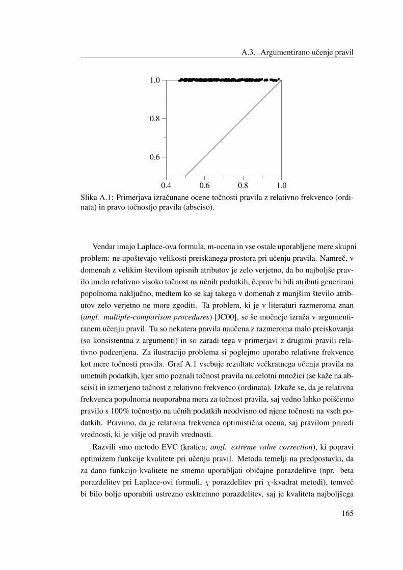
A.3. Argumentirano ucenje pravil
0.4 0.6 0.8 1.0
0.6
0.8
1.0
.......................................................................................................................................................................................................................................................................................................................................................................................................................................................................................................................•••• •• ••• ••• •• •• •• •• •• ••• •• • • •••• • • •• •• • • ••• •• ••• • •••• ••• ••• •• •• • ••• • ••• •• ••• •• • ••• ••• •• • •• •• ••••• •• • •••• • •• • •• • ••• •• •• • • •• •• • • •• •• •• •••• ••• •• •••• • •••••• •• •• •• ••• • • •• ••• •• ••• ••• •• •• • •• ••• ••• •• ••• •• •• • •••• •• •••• •• • ••• • •• •• ••• •• •• • •• • ••• •• • •• •• ••• • •• •• • •• •• •• • •• •• •• • ••• •• •• ••
Slika A.1: Primerjava izracunane ocene tocnosti pravila z relativno frekvenco (ordi-nata) in pravo tocnostjo pravila (absciso).
Vendar imajo Laplace-ova formula, m-ocena in vse ostale uporabljene mere skupniproblem: ne upostevajo velikosti preiskanega prostora pri ucenju pravila. Namrec, vdomenah z velikim stevilom opisnih atributov je zelo verjetno, da bo najboljse prav-ilo imelo relativno visoko tocnost na ucnih podatkih, ceprav bi bili atributi generiranipopolnoma nakljucno, medtem ko se kaj takega v domenah z manjsim stevilo atrib-utov zelo verjetno ne more zgoditi. Ta problem, ki je v literaturi razmeroma znan(angl. multiple-comparison procedures) [JC00], se se mocneje izraza v argumenti-ranem ucenju pravil. Tu so nekatera pravila naucena z razmeroma malo preiskovanja(so konsistentna z argumenti) in so zaradi tega v primerjavi z drugimi pravili rela-tivno podcenjena. Za ilustracijo problema si poglejmo uporabo relativne frekvencekot mere tocnosti pravila. Graf A.1 vsebuje rezultate veckratnega ucenja pravila naumetnih podatkih, kjer smo poznali tocnost pravila na celotni mnozici (se kaze na ab-scisi) in izmerjeno tocnost z relativno frekvenco (ordinata). Izkaze se, da je relativnafrekvenca popolnoma neuporabna mera za tocnost pravila, saj vedno lahko poiscemopravilo s 100% tocnostjo na ucnih podatkih neodvisno od njene tocnosti na vseh po-datkih. Pravimo, da je relativna frekvenca optimisticna ocena, saj pravilom priredivrednosti, ki je visje od pravih vrednosti.
Razvili smo metodo EVC (kratica; angl. extreme value correction), ki popravioptimizem funkcije kvalitete pri ucenju pravil. Metoda temelji na predpostavki, daza dano funkcijo kvalitete ne smemo uporabljati obicajne porazdelitve (npr. betaporazdelitev pri Laplace-ovi formuli, χ porazdelitev pri χ-kvadrat metodi), temvecbi bilo bolje uporabiti ustrezno esktremno porazdelitev, saj je kvaliteta najboljsega
165
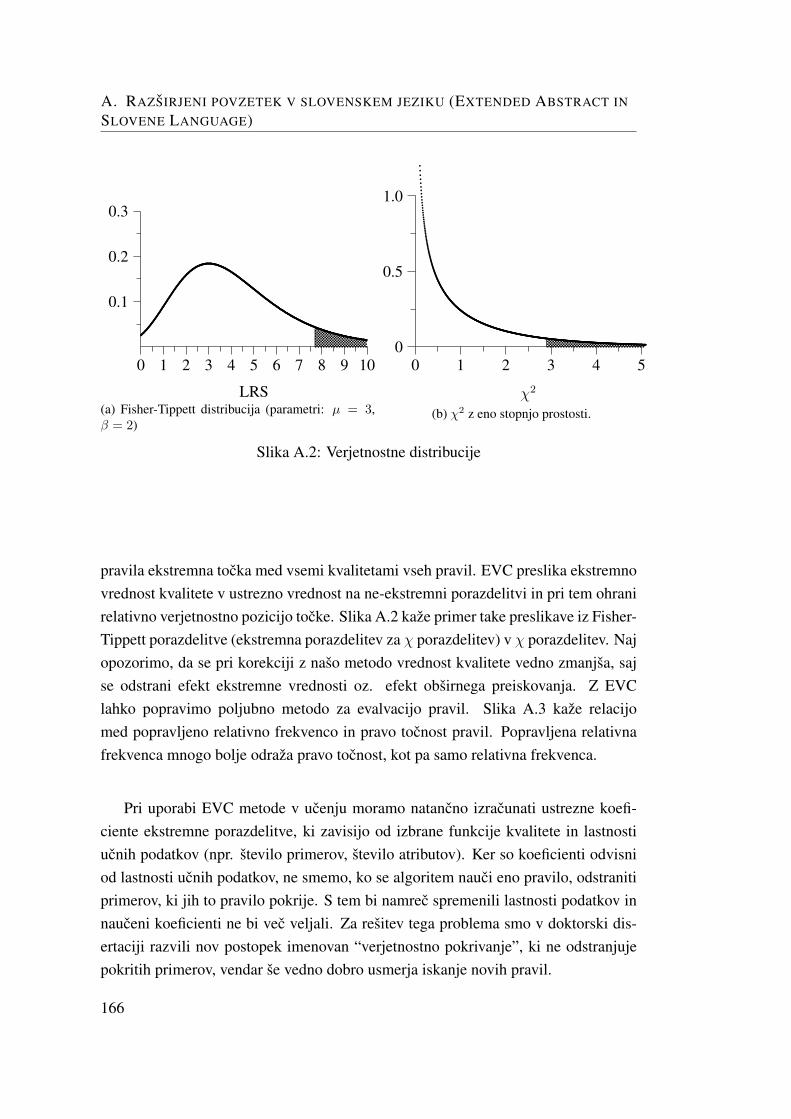
A. RAZSIRJENI POVZETEK V SLOVENSKEM JEZIKU (EXTENDED ABSTRACT IN
SLOVENE LANGUAGE)
0 1 2 3 4 5 6 7 8 9 10
LRS
0.1
0.2
0.3
.....................................................................................................................................................................................................
...................................................................................................................................................................................................................................................................................................................................................................................................................................................................................................................................................................................................................................................................................................................................................................................................................................
.......
.......
.......
.......
.......
....
......................................................................................................................................................................................
(a) Fisher-Tippett distribucija (parametri: µ = 3,β = 2)
0 1 2 3 4 5
χ2
0
0.5
1.0
....................................................................................................................................................................................................................................................................................................................................................................................................................................................................................................................................................................................................................................................................................................................................................................................................................................................................................................................................................................................................................................................................................................................................................................................................
(b) χ2 z eno stopnjo prostosti.
Slika A.2: Verjetnostne distribucije
pravila ekstremna tocka med vsemi kvalitetami vseh pravil. EVC preslika ekstremnovrednost kvalitete v ustrezno vrednost na ne-ekstremni porazdelitvi in pri tem ohranirelativno verjetnostno pozicijo tocke. Slika A.2 kaze primer take preslikave iz Fisher-Tippett porazdelitve (ekstremna porazdelitev za χ porazdelitev) v χ porazdelitev. Najopozorimo, da se pri korekciji z naso metodo vrednost kvalitete vedno zmanjsa, sajse odstrani efekt ekstremne vrednosti oz. efekt obsirnega preiskovanja. Z EVClahko popravimo poljubno metodo za evalvacijo pravil. Slika A.3 kaze relacijomed popravljeno relativno frekvenco in pravo tocnost pravil. Popravljena relativnafrekvenca mnogo bolje odraza pravo tocnost, kot pa samo relativna frekvenca.
Pri uporabi EVC metode v ucenju moramo natancno izracunati ustrezne koefi-ciente ekstremne porazdelitve, ki zavisijo od izbrane funkcije kvalitete in lastnostiucnih podatkov (npr. stevilo primerov, stevilo atributov). Ker so koeficienti odvisniod lastnosti ucnih podatkov, ne smemo, ko se algoritem nauci eno pravilo, odstranitiprimerov, ki jih to pravilo pokrije. S tem bi namrec spremenili lastnosti podatkov innauceni koeficienti ne bi vec veljali. Za resitev tega problema smo v doktorski dis-ertaciji razvili nov postopek imenovan “verjetnostno pokrivanje”, ki ne odstranjujepokritih primerov, vendar se vedno dobro usmerja iskanje novih pravil.
166
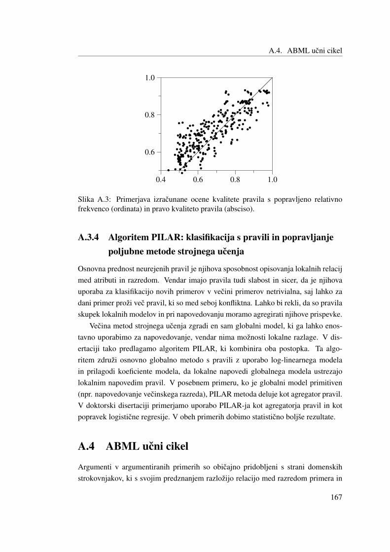
A.4. ABML ucni cikel
0.4 0.6 0.8 1.0
0.6
0.8
1.0
.......................................................................................................................................................................................................................................................................................................................................................................................................................................................................................................................
•
••
•
•
•
•
••
•
•
•
•
•
•
•
•
•
•
•
•
•
•
• •
•
•
•
•
•
•
•
•
•
••
••
••
••
•
•
•
•
•
•
•
•
•
••
•
•
•
•
•
•
•
•
•
•
•
••
•
••
••
•
•
•
•
•
•
•
•
•
•
•
•
••
•••
••
• •
•
••
••
•
••
•
•
•
••
•
•
•
•
•
•
•
•
•
•
••
•
• •
•
•
•
••
•
•
•
•
•
•
••
•
•
•
•
•
•
•
•
•
•
• •
•
•
•
••
••
•
•
•
•
•
•
•
•
•
• •
•
•
•
•
•
••
•
•
•
•
•
•
••
••
•
•
••
•
•
•
• ••
••
••
•
••
•
•
•
••
•
•
•
•
•
•
••
•
•
•
•
•
•
•
•
•
•• •
•
••
•
•
•
•
•
••
•
••
•
•
••
•
•
•
•
•
•
•
••
•
• ••
••
•
•
•
••
•
•
•
•
•
••
••
•
•
•
•
•
•
Slika A.3: Primerjava izracunane ocene kvalitete pravila s popravljeno relativnofrekvenco (ordinata) in pravo kvaliteto pravila (absciso).
A.3.4 Algoritem PILAR: klasifikacija s pravili in popravljanjepoljubne metode strojnega ucenja
Osnovna prednost neurejenih pravil je njihova sposobnost opisovanja lokalnih relacijmed atributi in razredom. Vendar imajo pravila tudi slabost in sicer, da je njihovauporaba za klasifikacijo novih primerov v vecini primerov netrivialna, saj lahko zadani primer prozi vec pravil, ki so med seboj konfliktna. Lahko bi rekli, da so pravilaskupek lokalnih modelov in pri napovedovanju moramo agregirati njihove prispevke.
Vecina metod strojnega ucenja zgradi en sam globalni model, ki ga lahko enos-tavno uporabimo za napovedovanje, vendar nima moznosti lokalne razlage. V dis-ertaciji tako predlagamo algoritem PILAR, ki kombinira oba postopka. Ta algo-ritem zdruzi osnovno globalno metodo s pravili z uporabo log-linearnega modelain prilagodi koeficiente modela, da lokalne napovedi globalnega modela ustrezajolokalnim napovedim pravil. V posebnem primeru, ko je globalni model primitiven(npr. napovedovanje vecinskega razreda), PILAR metoda deluje kot agregator pravil.V doktorski disertaciji primerjamo uporabo PILAR-ja kot agregatorja pravil in kotpopravek logisticne regresije. V obeh primerih dobimo statisticno boljse rezultate.
A.4 ABML ucni cikel
Argumenti v argumentiranih primerih so obicajno pridobljeni s strani domenskihstrokovnjakov, ki s svojim predznanjem razlozijo relacijo med razredom primera in
167
A. RAZSIRJENI POVZETEK V SLOVENSKEM JEZIKU (EXTENDED ABSTRACT IN
SLOVENE LANGUAGE)
vrednostimi atributov. Zato ne moremo pricakovati, da bi strokovnjaki argumentiralivse ucne primere, saj za kaj takega ne bi imeli casa. Pripraviti jim moramo izbiroucnih primerov, ki bodo z argumenti obcutno vplivali na kvaliteto naucene hipoteze.Na primer, ne bi bilo smiselno argumentirati primerov, ki jih metoda ze sama dobrorazlozi.
V ta namen smo razvili iterativni postopek za odkrivanje in argumentiranje kriticnihprimerov, ki ga imenujemo ABML ucni cikel. Cikel zacne z “navadnimi” ucnimiprimeri (brez argumentov) in v vsakem ciklu doda argument k enemu ucnemu primeru.Postopek, ki se ustavi, ko ne najde vec novega kriticnega primera, ima stiri korake:
1. Nauci se hiptezo z ABML na danih ucnih podatkih.
2. Poisci kriticni primer in ga predlozi domenskemu strokovnjaku za argumentacijo.Ce kriticnega primera ne najdemo, se postopek ustavi.
3. Domenski strokovnjak razlozi dani primer z argumenti v naravnem jeziku. Tiargumenti se rocno prevedejo v formalne argumente, ki jih sprejema ABMLmetoda, in dodajo h kriticnemu ucnemu primeru.
4. Vrni se na korak 1.
Osnovna ideja koraka 2 je poiskati primer, ki ga metoda ne more uspesno ra-zloziti, z drugimi besedami, metoda napacno napove razred primera. V najbolj enos-tavni izvedbi za iskanje teh primerov se naucimo modela in ga testiramo na ucnihpodatkih. Napacno klasificirani primeri tako postanejo kriticni primeri. Problem tegapristopa je, da ne deluje pri metodah z lastnostjo prevelikega prilagajanja (angl. over-fitting), kjer je bolje uporabiti metodo kriznega preverjanja za odkrivanje kriticnihprimerov.
A.5 Eksperimenti in aplikacije
Za evalvacijo metode ABCN2 bomo v tem razdelku predstavili vrsto eksperimentovin aplikacij. To je edini mozni nacin evalvacije, saj korektna statisticna primerjava niprakticno izvedljiva, ker bi potrebovali mnogo ucnih domen in za vsako domenskegastrokovnjaka, ki bi razlagal ucne primere. Z izvedenimi eksperimenti in aplikacijamiodgovorimo na nekaj kljucnih vprasanj, ki se ticejo evalvacije metode:
• Ali so hipoteze naucene iz argumentiranih podatkov boljse kot hipoteze iznavadnih (neargumentiranih podatkih) s stalisca tocnosti in razumljivosti?
168
A.5. Eksperimenti in aplikacije
• Kako ucinkovita je metoda za izbiro kriticnih primerov?
• Ali oziroma kako tezko je domenski strokovnjakom podajati znanje v oblikiargumentov?
• Ali lahko rekonstruiramo (in izboljsamo) dano bazo znanja, kjer se trenutnoznanje v bazi uporablja kot izvor argumentov?
• Ali lahko (in kako) uporabimo argumente, ki omenjajo informacijo, ki ni za-pisana v atributih?
• Ali lahko argumente avtomatsko pridobimo iz neodvisne literature (npr. inter-net)?
• Kako napake argumentov vplivajo na tocnost naucenih hipotez?
A.5.1 Klasifikacija zivali
Prvi eksperiment z ABCN2 smo izvedli na domeni za klasifikacijo zivali, kjer je ciljklasificirati zivali glede na njihov tip v zivalskem drevesu (domena ZOO [AN07]).Domena vsebuje 101 zival, vsaka je opisana s sedemnajstimi atributi in klasificiranav enega od naslednjih razredov: sesalec, ptic, plazilec, riba, dvozivka, insekt, os-talo. Ta domena je zelo ustrezna za zacetno evalvacijo, ker ne potrebujemo pravegadomenskega strokovnjaka, ampak lahko ustrezne argumente kar poiscemo iz encik-lopedije.
Domeno smo razdelili na ucno mnozico (70%) in testno mnozico (30%). Najprejsmo se naucili pravil brez uporabe argumentov, kjer smo z ABCN2 na testni mnozicidosegli tocnost priblizno 90%. Nato smo znotraj ABML ucnega cikla identificiralitri kriticne primere:
1. Prvi kriticni primer je bil zelva. Zelva je plazilec in za plazilce je med drugimznacilno, da imajo hrbtenjaco in lezejo jajca (argument: zelva je plazilec, kerhrbtenjaca=da in leze jajca=da). S pomocjo tega argumenta je ABCN2 dodalpravilo (poudarjen del pravila izhaja iz argumenta):
CE hrbtenjaca=da IN leze jajca=da INvodna zival=ne IN perje=ne POTEM tip=plazilec
169
A. RAZSIRJENI POVZETEK V SLOVENSKEM JEZIKU (EXTENDED ABSTRACT IN
SLOVENE LANGUAGE)
2. Naslednji kriticni primer je bila morska kaca (plazilec). V opisnih atributihtega primera pise, da morska kaca ne diha, ceprav v vseh knjigah pise, damorska kaca diha s pljuci. Ocitno gre pri tem primeru za napako v podatkih.
3. Zadnji kriticni primer je bil mocerad (dvozivka). Nas argument je: moceradje dvozivka, ker ima hrbtenjaco, leze jajca in mora ziveti v vlaznem okolju zaprezivetje. Pravilo nauceno iz tega argumenta je bilo:
CE hrbtenjaca=da IN leze jajca=da IN vodna zival=daIN stevilo nog=4 POTEM tip=dvozivka
V eksperimentu smo torej vse skupaj dodali dva argumenta in oba sta bila nepopolna,saj je ABCN2 oba specializiral z dodatnimi pogoji. Koncna tocnost pravil na ucnimnozici je bila 100%. Eksperiment nazorno prikazuje ucinkovitost ABML ucnegacikla, saj smo s pomocjo samo dveh argumentov uspeli povecati tocnost za 10%. Po-leg tega so nova pravila bolj v skladu s strokovnim znanjem - enciklopedijo in s temze na prvi pogled izgledajo pravilneje. Izkazalo se je tudi, da je ABML ucni cikelprimeren za odkrivanje napak v ucnih primerih.
A.5.2 Odobritev socialne pomoci
V tem delu bomo povzeli rezultate eksperimenta z ABCN2 v pravni domeni: odobritevsocialne pomoci za obisk druzinskih clanov v bolnici [MvBC+06]. Domena je sicerumetna, vendar je bila zaradi realnosti atributov in primerov veckrat citirana v pravniliteraturi, ki so jo v preteklosti resevali z razlicnimi tehnikami strojnega ucenja.
Tocnost osnovne CN2 metode brez uporabe argumentov je zelo visokih 99%. Posedmih ABML ciklih se je tocnost z uporabo ABCN2 povecala na 99.8%. Ker jebila tocnost ucenja brez argumentov ze zelo visoka, seveda ni mozno dobiti mnogoboljse rezultate z argumentiranim ucenjem. Glavna prednost ABCN2 v tej domenije razumljivost naucenih pravil, saj so bila koncna pravila mnogo bolj razumljivadomenskemu strokovnjaku (Trevor Bench Capon), ker so vsebovala njegove razlageprimerov. Izkazalo se je tudi, da je ABCN2 mnogo bolj odporna na sum od ostalihmetod, kar je kljucnega pomena za tak tip aplikacij, saj odlocitve administracije vse-bujejo veliko napacnih odlocitev.
170

A.5. Eksperimenti in aplikacije
CN2 ABCN2 NB C4.5 LogReg
0.6
0.65
0.7
0.75
0.8
0.85
class: DEATH (yes/no)
AU
C
Slika A.4: Povprecne vrednosti in standardne napake AUC.
A.5.3 Prognostika infekcije med starejsimi obcani
V tej domeni smo z ABCN2 razvili model za pomoc zdravnikom pri ocenjevanjukriticnosti infekcije med starejsimi obcani. Na podlagi tega modela se naj bi zdravnikiodlocili, ali pacient ostane v bolnici ali lahko oddide domov. Podatke smo dobili izljubljanske klinike za infekcijske bolezni in vkljucujejo vse ljudi starejse od 65 let,ki so prisli v bolnico med 1.junijem 2004 in 1.junijem 2005 zaradi okuzbe. Razredoznacuje ali je pri pacientu v roku 30 dni po nastopu okuzbe nastopila smrt.
Tu je domenski strokovnjak (zdravnik) argumentiral vse pozitivne primere (kjerje pacient preminil) in nobenega negativnega. Z uporabo argumentov je bila ABCN2signifikantno boljsa metoda (glede na klasifikacijsko tocnost, AUC in Brier Score)od CN2, naivnega Bayesa in logisticne regresije (glej sliko A.4 za primerjavo AUC).Kljub boljsim rezultatom ucenja z argumenti in upostevaje, da so bila naucena prav-ila konsistentna s strokovnim znanjem, se domenskemu strokovnjaku (dr. JernejaVidecnik, dr. med.) ABCN2 pravila niso zdela bolj (niti ne manj) smiselna od pravildobljenih z navadnim CN2. Ta anomalija nastane zaradi kratke dolzine argumentov.Vsi argumenti so namrec vsebovali le en razlog, na primer:
smrt = da ker frekvenca dihanja >= 16
171

A. RAZSIRJENI POVZETEK V SLOVENSKEM JEZIKU (EXTENDED ABSTRACT IN
SLOVENE LANGUAGE)
Ker tak argument omeji preiskovanje razmeroma malo (pravilo mora vsebovati le tapogoj, ostali so poljubni) in ker so bila pravila razmeroma dolga (3-5 pogojev napravilo), se pravila niso obcutno razlikovala po razumljivosti. Vseeno pa so ti kratkiargumenti se vedno omogocili bolj tocno ucenje.
A.5.4 Prognostika bolezni srca
Domena za prognostiko bolezni srca (SAHeart) [RdPB+83] je prosto dostopna inopisuje 462 moskih iz Juzne Afrike. Ucni primeri so opisani z devetimi atributi:krvni pritisk, kajenje, holesterol, debelost, druzinska anamneza, stil zivljenja (type-A), kozna guba, alkohol in starost ter razredom chd, ki oznacuje, ce pacient ima srcnobolezen ali ne.
Pri tem poskusu nismo imeli na voljo domenskih strokovnjakov. Zanimalo nas je,ce lahko z uporabo nasega splosnega znanja (ki je lahko napacno) o srcnih boleznihpomagamo ABCN2, da se nauci bolj tocne hipoteze. Ta test sluzi tudi kot preizkusABCN2, kako obcutljiva je metoda na napake v argumentih. Po desetih iteracijahABML ucnega cikla se je klasifikacijska tocnost ABCN2 zvisala iz zacetnih 71% na75%, Brier Score se je izboljsal iz 0.37 na 0.36, le AUC se ni spremenila. Ne glede nato, da nasi argumenti niso bili popolni, smo se vedno uspeli izboljsati zacetni model.To je pomembna ugotovitev, saj kaze, da predznanje ne rabi biti popolnoma pravilnoin je lahko se vedno uporabno. Seveda se zavedamo, da bi kardiologovi argumentiverjetno se bolj izboljsali tocnost naucenega modela.
A.5.5 Odobravanje kredita (Japanese Credit ScreeningDatabase)
Japonska domena za odobravanje kredita opisuje 125 prosilcev kredita z desetimiatributi in razredom, ki oznacuje, ce je oseba dobila kredit ali ne. Domeni je prilozenotudi suboptimalno domensko znanje (6 pravil, ki jih posamezniki v bankah uporabl-jajo za podeljevanje kredita), ki doseze 83% klasifikacijsko tocnost na ucnih primerih.V tem poskusu smo uporabili to domensko znanje kot trenutno bazo znanja, ki namsluzi kot izvor argumentov. Cilj ucenja z ABCN2 je bil (a) rekonstruirati to bazoznanja in jo (b) izboljsati.
Brez argumentov se je ABCN2 naucil le tri pravila, ki so dosegala 76% klasi-fikacijsko tocnost. Po petih iteracijah ABML ucnega cikla je model obsegal 7 pravilin 89% klasifikacijsko tocnost. S tem smo popolnoma uspeli rekonstruirati originalno
172

A.5. Eksperimenti in aplikacije
bazo znanja, saj je, od vseh sedmih naucenih pravil, sest pravil popolnoma ustrezalooriginalni bazi znanja. Sedmo pravilo tako predstavlja dodatno pridobljeno znanje,ki je se izboljsalo klasifikacijsko tocnost iz 83% na 89%.
A.5.6 Konstrukcija kompleksnih sahovskih konceptov
Dandanasnji racunalniski programi za igranje saha so izredno dobri pri igranju saha,vendar skorajda neuporabni za ucenje saha ali razlago sahovskih partij. Vsako pozi-cijo oznacijo s stevilosko vrednostjo, ki oznacuje agregirano situacijo pozicije. Naprimer, vrednost 1.20 naj bi pomenila, da je beli v prednosti za dobrega kmeta, cepravni nujno, da tudi dejansko ima kmeta vec; lahko ima iniciativo v napadu, boljsepostavljene lovce, itd. Trenutni programi ne znajo razumljivo razloziti te vrednosticloveku, zakaj je beli v boljsem polozaju. Nedavno smo razvili sistem za ucenjesaha [SMG+06], ki razlaga vrednosti hevristicne funkcije s spremembami vrednostiposameznih atributov v evaluaciji pozicije. Izkaze se, da hevristicne funkcije vglavnem uporabljajo primitivne sahovske koncepte (npr. stevilo kmetov, mobilnostifigur, itd.), ki pa niso dovolj za razumevanje splosnih sahovskih pozicij.
Naslednji eksperiment demonstrira uporabnost ABCN2 za ucenje kompleksnihsahovskih konceptov. Izbrali smo koncept slabega lovca. Vzeli smo 200 sahovskihpozicij in jih opisali z atributi, ki so tipicno uporabljeni v hevristicnih funkcijah zaigranje saha. Jana Krivec (zenska velemojstrica) in Matej Guid (FIDE mojster) stav vsaki od teh pozicij ocenila lovca kot “slabi lovec” ali “dober lovec” in pri temuporabljala njuno sahovsko predznanje.
Za zacetek sta domenska strokovnjaka Guid in Krivec poskusila z uporabo danihatributov rocno generirati pravila, ki bi razlikovala dobrega od slabega lovca. Vendarse je to izkazalo za zelo tezek problem, saj so njuna pravila delovala relativno slabo,dosegla so samo 59% klasifikacijsko tocnost. ABCN2 je na danih podatkih (brezargumentov) dosegla mnogo boljso tocnost 72%. Nato smo izvedli 8 ABML ucnihciklov in pri tem dodali 7 argumentov. V nekaterih kriticnih primerih Guid in Krivecnista uspela razloziti danih pozicij s samo obstojecimi atributi, zato smo v procesudodali nekaj dodatnih atributov. Tocnost koncnega modela je dosegla visokih 95%.Iz slike A.5 je ocitna ucinkovitost algoritma za izbiro kriticnih primerov, saj prvihnekaj argumentov najbolj poveca tocnost naucenih pravil. Vidi se tudi, da je doda-janje atributov, ki so bili predlagani z argumenti, mnogo prispevalo k tocnosti ostalihmetod. ABML ucni cikel je torej dober postopek tudi za odkrivanje manjkajocihatributov. Ta eksperiment jasno kaze izboljsanje klasifikacijske tocnosti z uporabo
173
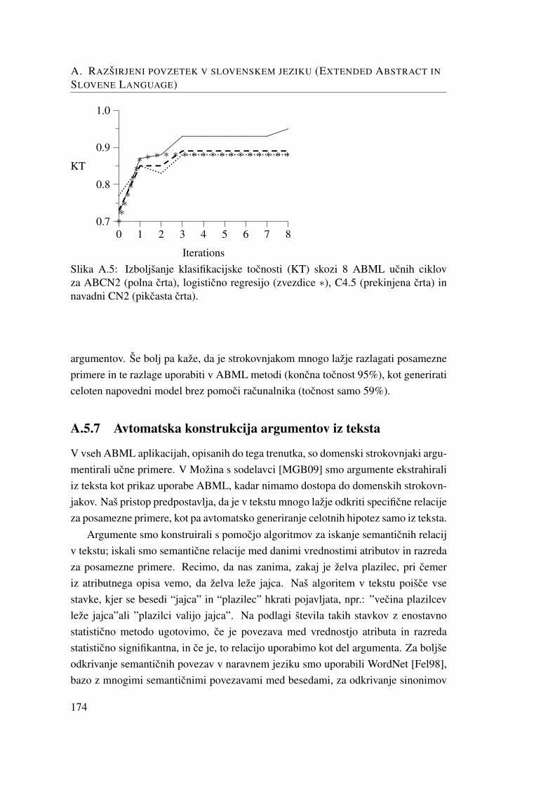
A. RAZSIRJENI POVZETEK V SLOVENSKEM JEZIKU (EXTENDED ABSTRACT IN
SLOVENE LANGUAGE)
0 1 2 3 4 5 6 7 8
Iterations
0.7
0.8
0.9
1.0
KT
.............................................................................................................................................................................................................
................................................................................................................................................................................................................................................................................................................................
......................................
....................
∗∗∗∗∗∗∗∗ ∗ ∗ ∗ ∗ ∗ ∗ ∗ ∗ ∗ ∗ ∗ ∗ ∗ ∗ ∗ ∗
.............................................................................. ............. ............. .............
............. ............. ............. ............. ............. ............. ............. ............. ............. ............. ............. ............. .............
.........................
.............................................
Slika A.5: Izboljsanje klasifikacijske tocnosti (KT) skozi 8 ABML ucnih ciklovza ABCN2 (polna crta), logisticno regresijo (zvezdice ∗), C4.5 (prekinjena crta) innavadni CN2 (pikcasta crta).
argumentov. Se bolj pa kaze, da je strokovnjakom mnogo lazje razlagati posamezneprimere in te razlage uporabiti v ABML metodi (koncna tocnost 95%), kot generiraticeloten napovedni model brez pomoci racunalnika (tocnost samo 59%).
A.5.7 Avtomatska konstrukcija argumentov iz teksta
V vseh ABML aplikacijah, opisanih do tega trenutka, so domenski strokovnjaki argu-mentirali ucne primere. V Mozina s sodelavci [MGB09] smo argumente ekstrahiraliiz teksta kot prikaz uporabe ABML, kadar nimamo dostopa do domenskih strokovn-jakov. Nas pristop predpostavlja, da je v tekstu mnogo lazje odkriti specificne relacijeza posamezne primere, kot pa avtomatsko generiranje celotnih hipotez samo iz teksta.
Argumente smo konstruirali s pomocjo algoritmov za iskanje semanticnih relacijv tekstu; iskali smo semanticne relacije med danimi vrednostimi atributov in razredaza posamezne primere. Recimo, da nas zanima, zakaj je zelva plazilec, pri cemeriz atributnega opisa vemo, da zelva leze jajca. Nas algoritem v tekstu poisce vsestavke, kjer se besedi “jajca” in “plazilec” hkrati pojavljata, npr.: ”vecina plazilcevleze jajca”ali ”plazilci valijo jajca”. Na podlagi stevila takih stavkov z enostavnostatisticno metodo ugotovimo, ce je povezava med vrednostjo atributa in razredastatisticno signifikantna, in ce je, to relacijo uporabimo kot del argumenta. Za boljseodkrivanje semanticnih povezav v naravnem jeziku smo uporabili WordNet [Fel98],bazo z mnogimi semanticnimi povezavami med besedami, za odkrivanje sinonimov
174
A.6. Zakljucek
in raznovrstnih izpeljank (npr. plazilec→ plazilci).
Pristop smo testirali na domeni za klasifikacijo zivali. Vsi argumenti so bili av-tomatsko konstruirani iz clankov na Wikipediji.† Za evalvacijo smo 10-krat ponovili10-kratno krizno preverjanje in vsakic generirali argumente za prav vse ucne primere.Brez argumentov je ABCN2 v povprecju dosegla 94.5% klasifikacijsko tocnost, a zargumenti 96.7%, kar je statisticno boljsi rezultat. ABCN2 se nauci boljsega mod-ela tudi od ostalih standardnih metod strojnega ucenja (npr. naivni Bayes 92.6%,SVM 90%, C4.5 92.57%). Rezultati se v tem eksperimentu rahlo razlikujejo od prejopisanega eksperimenta na tej domeni, zaradi spremenjene tehnike evalvacije.
A.5.8 Vpliv napacnih argumentov na tocnost hipoteze
Ali lahko napacni (oz. slabi) argumenti poslabsajo tocnost koncnega modela gledena originalni model? Ker argumenti omejujejo prostor sprejemljivih hipotez, bi lahkopricakovali, da bodo napacni argumenti omejili prostor iskanja na prostor slabihhipotez in s tem onemogocili ABCN2 poiskati dober koncni model.
Z obseznim eksperimentiranjem smo pokazali, da argumenti ne morejo poslabsatimodela dokler so argumenti boljsi ali enako dobri kot nakljucno generirani argu-menti. Izkaze se namrec, da nakljucno generirani argumenti v povprecju ne poslabsajotocnosti koncnega modela, iz cesar lahko sklepamo, da tudi argumenti, ki so boljsiod nakljucnih ne bodo poslabsali modela. Mozno bi bilo s pazljivo konstruiran-imi argumenti, ki so slabsi od nakljucnih, poslabsati koncni model. Vendar, kertega od domenskih strokovnjakov, ki si zelijo dobiti cim boljse modele, ne moremopricakovati, lahko trdimo, da napacni (oz. slabi) argumenti ne poslabsajo tocnostikoncnega modela.
A.6 Zakljucek
V disertaciji smo definirali argumentirano strojno ucenje, ki zdruzuje strojno ucenjez nekaj koncepti iz argumentacijske teorije. Argumentacijska teorija je posebna vejalogike, ki ne zahteva nokonfliktnosti med pravili in dejstvi ter s tem omogoca enos-tavno pridobivanje ekspertnega znanja in simulira clovesko sklepanje. V argumen-tiranem strojnem ucenju se domenski strokovnjak fokusira na konkretni ucni primerin poskusa z argumentom razloziti relacijo med razredom in atributi.
†http://en.wikipedia.org
175
A. RAZSIRJENI POVZETEK V SLOVENSKEM JEZIKU (EXTENDED ABSTRACT IN
SLOVENE LANGUAGE)
Ucni primer, razlozen z argumentom, se imenuje argumentirani ucni primer. Vargumentiranem strojnem ucenju se ucimo iz argumentiranih ucnih podatkov, kjerzahtevamo, da je naucena hipoteza konsistentna z danimi ucnimi podatki in nji-hovimi argumenti. Na podlagi osnovih principov argumentiranega ucenja smo razvilimetodo ABCN2, ki je razsirjenja razlicica znanega algoritma za ucenje pravil CN2.
ABCN2 smo se dodatno razsirili z metodi EVC in PILAR. Prva metoda kori-gira ocenjeno tocnost pravil glede na stevilo pregledanih pravil v postopku ucenja.PILAR je klasifikacijska metoda, ki uposteva korekcije metode EVC in zgradi log-linearni globalni model iz naucenih pravil. Obe metodi sta se izkazali kot pomembniizboljsavi ABCN2, vendar povecujeta zahtevani cas ucenja. Slednje nas ne moti, sajje sam cas ucenja se vedno zanemarljivo majhen v primerjavi s casom, ki ga porabimoza sodelovanje s strokovnjakom.
Predlagani algoritem za izbiro kriticnih primerov vedno izbere primer, ki gatrenutna metoda napacno klasificira. Vprasanje za prihodnje delo je, ce je to vednosmiselno. Namrec, metoda lahko napacno klasificira tudi osamelec (angl. outlier), kiga strokovnjaki zelo verjetno ne bodo znali razloziti oz., ce bodo nasli razlago, je le-talahko izsiljena. Ali je mozno za dani ucni primer oceniti verjetnost, da bo domenskistrokovnjak poznal odgovor? S tem vprasanjem se bomo ukvarjali v prihodnosti.
Z eksperimenti smo ugotovili naslednje prednosti ABML pristopa in metodeABCN2:
• Domenskim strokovnjakom je lazje argumentirati specificne primere kot poda-jati splosno domensko znanje.
• Kriticni primeri, ki bi z argumenti najbolj vplivali na tocnost modela, so av-tomatsko odkriti znotraj ABML ucnega cikla.
• S protiprimeri, ki spodbijajo dane argumente, omogocimo strokovnjakom izpopol-nitev njihovih argumentov. V enem od eksperimentov (ucenje sahovskih kon-ceptov) se je izkazalo, da s tem celo izboljsamo znanje strokovnjakov, saj sedo tega trenutka niso zavedali teh protiprimerov.
• Pravila naucena z ABCN2 so strokovnjakom bolj razumljiva kot pravila naucenasamo s CN2.
• V stevilnih eksperimentih in aplikacijah je ABCN2 dosegel boljso klasifikaci-jsko tocnost (in tudi druge mere kvalitete) kot CN2.
176
A.6. Zakljucek
V enem od zadnjih eksperimentov smo razvili metodo za avtomatsko odkrivanjeargumentov iz teksta. Ideja tega postopka je odkriti argumente za dane primere, kadarnam domenski strokovnjak ni na voljo. Trenutno smo s tem postopkom dobili dobrerezultate na enem eksperimentu in v nadaljnjem delu planiramo ta princip apliciratise na druge domene.
Pricujoce delo opisuje le eno implementacijo ABML koncepta; za ucenje neure-jenih pravil. Nase prepricanje je, da bi se ta koncept izkazal za se bolj uporabnega vkompleksnejsih domenah (npr. razumevanje teksta, grafov, zaporedij), kjer je prostorhipotez obicajno se veliko vecji in je brez uporabe predznanja prakticno nemogoceizvesti uspesno ucenje. Verjetno najbolj primerna metoda za ucenje v teh domenah jeILP, saj omogoca opis kompleksnih relacij (rekurzivne relacije, relacije med primeri,itd.) v nauceni hipotezi. V doktorski disertaciji smo opisali nekaj idej za razvojmetode AB-ILP (argument based ILP). V nadaljnjem delu nameravamo te ideje im-plementirati in jih testirati na realnih domenah.
177


A.6. Zakljucek
179

Bibliography
[ACE] ACE – Automatic Content Extraction, http://www.nist.gov/speech/tests/ace.
[ADZ+07] Noriaki Aoki, Janez Demsar, Blaz Zupan, Martin Mozina, Ernesto A. Pretto,Jun Oda, Hiroshi Tanaka, Katsuhiko Sugimoto, Toshiharu Yoshioka, and Tsug-uya Fukui. Predictive model for estimating risk of crush syndrome : a datamining approach. The Journal of trauma, injury, infection, and critical care,62(4):940–945, 2007.
[AN07] A. Asuncion and D.J. Newman. UCI machine learning repository, 2007.
[AR03] Kevin D. Ashley and Edwina L. Rissland. Law, learning and representation.Artificial Intelligence, 150:17–58, 2003.
[Atk89] Kendall E. Atkinson. An Introduction to Numerical Analysis. John Wiley andSons, New York, 1989.
[BA03] Stefanie Bruninghaus and Kevin D. Ashley. Predicting the outcome of case-based legal arguments. In G. Sartor, editor, Proceedings of the 9th Interna-tional Conference on Artificial Intelligence and Law (ICAIL), pages 233–242,Edinburgh, United Kingdom, June 2003.
[BC91a] Trevor J. M. Bench-Capon. Knowledge-based systems and legal applications.Academic Press Professional, Inc., San Diego, CA, USA, 1991.
[BC91b] Trevor J.M. Bench-Capon. Knowledge Based Systems and Legal Applications,chapter Knowledge Based Systems Applied To Law: A Framework for Discus-sion, pages 329–342. Academic Press., 1991.
[BC93] Trevor J.M. Bench-Capon. Neural nets and open texture. In Fourth Interna-tional Conference on AI and Law, pages 292–297, Amsterdam, 1993. ACMPress.
181
BIBLIOGRAPHY
[BCC00] Trevor J.M. Bench-Capon and Frans Coenen. An experiment in discover-ing association rules in the legal domain. In 11th International Workshop onDatabase and Expert Systems Applications, pages 1056–1060, Los Alamitos,2000. IEEE Computer Society.
[BM04] Ivan Bratko and Martin Mozina. Argumentation and machine learning. In:Deliverable 2.1 for the ASPIC project, 2004.
[BM05] Razvan Bunescu and Raymond J. Mooney. Subsequence kernels for relationextraction. In Proceedings of the 19th Conference on Neural Information Pro-cessing Systems, Vancouver, British Columbia, 2005.
[Boo89] John H. Boose. A survey of knowledge acquisition techniques and tools.Knowledge Acquisition, 1(1):3–37, 1989.
[Bra01] Ivan Bratko. PROLOG Programming for Artificial Intelligence. Third edition.Addison-Wesley, Harlow, England, 2001.
[Bre96] Leo Breiman. Bagging predictors. Machine Learning, 24:123–140, 1996.
[Bre01] Leo Breiman. Random forests. Machine Learning, 45(1):5–32, 2001.
[Bri50] Glenn W. Brier. Verification of forecasts expressed in terms of probabilities.Mon. Wea. Rev., 78, 1950.
[BS91] Wray Buntine and David Stirling. Interactive induction. Machine intelligence,12:121–137, 1991.
[Bud01] Raluca Budiu. The role of background knowledge in sentence processing. PhDthesis, School of Computer Science, Carnegie Mellon University, Pittsburgh,PA., 2001. Available as Technical Report No. CMU-CS-01-148.
[BZ04] Marko Bohanec and Blaz Zupan. A function-decomposition method for de-velopment of hierarchical multi-attribute decision models. Decision SupportSystems, 36:215–233, 2004.
[CAL94] David Cohn, Les Atlas, and Richard Ladner. Improving generalization withactive learning. Mach. Learn., 15(2):201–221, 1994.
[CB91] Peter Clark and Robin Boswell. Rule induction with CN2: Some recent im-provements. In Machine Learning - Proceeding of the Fifth Europen Confer-ence (EWSL-91), pages 151–163, Berlin, 1991.
182

Bibliography
[Ces90] Bojan Cestnik. Estimating probabilities: A crucial task in machine learning. InProceedings of the Ninth European Conference on Artificial Intelligence, pages147–149, 1990.
[Chk03] Timothy Chklovski. Using Analogy to Acquire Commonsense Knowledge fromHuman Contributors. PhD thesis, MIT Artificial Intelligence Laboratory, 2003.
[CL01] Chih-Chung Chang and Chih-Jen Lin. LIBSVM: a library for support vectormachines, 2001. Software available at http://www.csie.ntu.edu.tw/
˜cjlin/libsvm.
[Cla88] Peter Clark. Representing arguments as background knowledge for constrain-ing generalisation. In Derek Sleeman, editor, Third European Working Sessionon Learning, October 1988.
[CM93] Peter Clark and Stan Matwin. Using qualitative models to guide inductivelearning. In Proceedings of the tenth international machine learning confer-ence, 1993.
[CN89] Peter Clark and Tim Niblett. The CN2 induction algorithm. Machine LearningJournal, 4(3):261–283, 1989.
[Coh94] William W. Cohen. Grammatically biased learning: Learning logic pro-grams using an explicit antecedent description language. Artificial Intelligence,68:303–366, 1994.
[Coh95] William W. Cohen. Fast effective rule induction. In In Proceedings of theTwelfth International Conference on Machine Learning, pages 115–123. Mor-gan Kaufmann, 1995.
[Col01] Stuart Coles. An Introduction to Statistical Modeling of Extreme Values.Springer, 1 edition, december 2001.
[Coo94] Nancy J. Cooke. Varieties of knowledge elicitation techniques. Int. J. Hum.-Comput. Stud., 41(6):801–849, 1994.
[CRL00] Daniela V. Carbogim, David Robertson, and John Lee. Argument-based appli-cations to knowledge engineering. Knowl. Eng. Rev., 15(2):119–149, 2000.
[CS99] William W. Cohen and Yoram Singer. A simple, fast, and effective rule learner.In In Proceedings of the Sixteenth National Conference on Artificial Intelli-gence, pages 335–342. AAAI Press, 1999.
183

BIBLIOGRAPHY
[dAT01] Pedro de Almeida and Luıs Torgo. The use of domain knowledge in featureconstruction for financial time series prediction. In Progress in Artificial Intel-ligence, pages 29–39, 2001.
[DCP93] Saso Dzeroski, Bojan Cestnik, and Igor Petrovski. Using the m-estimate inrule induction. Journal of Computing and Information Technology, 1(1):37–46, 1993.
[Dem06] Janez Demsar. Statistical comparisons of classifiers over multiple data sets.Journal of Machine Learning Research, 7:1–30, 2006.
[Die02] Thomas G. Dietterich. The Handbook of Brain Theory and Neural Networks,Second Edition, chapter Ensemble Learning, pages 405–409. The MIT Press,2002.
[DKS08] Krzysztof Dembczynski, Wojciech Kotlowski, and Roman Slowinski. Maxi-mum likelihood rule ensembles. In ICML ’08: Proceedings of the 25th interna-tional conference on Machine learning, pages 224–231, New York, NY, USA,2008. ACM.
[Dom99] Pedro Domingos. The role of occam’s razor in knowledge discovery. DataMining and Knowledge Discovery, 3(4):409–425, 1999.
[Dun93] Ted E. Dunning. Accurate methods for the statistics of surprise and coinci-dence. Computational Linguistics, 19(1):61–74, 1993.
[Dun95] Phan M. Dung. On the acceptability of arguments and its fundamental role innonmonotonic reasoning, logic programming, and n-person games. ArtificialIntelligence, 77:321–357, 1995.
[DZ04] Janez Demsar and B. Zupan. Orange: From experimental machine learningto interactive data mining. White Paper [http://www.ailab.si/orange], Faculty ofComputer and Information Science, University of Ljubljana, 2004.
[Edv95] Lilian Edvards. Modelling law using a feminist theoretical perspective. Law,Computers and Artificial Intelligence, 4:95–110, 1995.
[Fei84] Edward A. Feigenbaum. Knowledge engineering: the applied side of artificialintelligence. In Proc. of a symposium on Computer culture: the scientific,intellectual, and social impact of the computer, pages 91–107, New York, NY,USA, 1984. New York Academy of Sciences.
184
Bibliography
[Fei03] Edward A. Feigenbaum. Some challenges and grand challenges for computa-tional intelligence. Source Journal of the ACM, 50(1):32–40, 2003.
[Fel98] Christiane Fellbaum. WordNet. An Electronic Lexical Database. MIT Press,1998.
[FF05] Johannes Furnkranz and Peter A. Flach. Roc ’n’ rule learning – towards abetter understanding of covering algorithms. Machine Learning, 58(1):39–77,January 2005.
[For86] Richard Forsyth. Machine learning for expert systems. Machine Learning,1(1):3–37, 1986.
[FP08] Jerome H. Friedman and Bogdan E. Popescu. Predictive learning via rule en-sembles. Ann. Appl. Stat., 2(3):916–954, 2008.
[FPM+] Paolo Frasconi, Andrea Passerini, Stephen Muggleton, , and Huma Lodhi.Declarative kernels. Technical Report RT 2/2004, Dipartimento di Sistemi eInformatica, Universit‘a di Firenze, 2004.
[FR86] Richard Forsyth and Roy Rada. Machine learning: applications in expert sys-tems and information retrieval. Halsted Press, New York, NY, USA, 1986.
[FS97] Yoav Freund and Robert E. Schapire. A decision-theoretic generalization of on-line learning and an application to boosting. Journal of Computer and SystemSciences, 55(1):119–139, 1997.
[FT28] Ronald A. Fisher and Leonard H.C. Tippett. Limiting forms of the frequencydistribution of the largest and smallest member of a sample. Proc. Camb. Phil.Soc., 24:180–190, 1928.
[Fur97] Johannes Furnkranz. Pruning algorithms for rule learning. Machine Learning,27(2):139–171, 1997.
[GC04a] Sergio A. Gomez and Carlos I. Chesnevar. Integrating defeasible argumenta-tion and machine learning techniques. Technical report, Universidad Nacionaldel Sur, 2004.
[GC04b] Sergio A. Gomez and Carlos I. Chesnevar. Integrating defeasible argumenta-tion with fuzzy art neural networks for pattern classification. Journal of Com-puter Science and Technology, 4(1):45–51, April 2004.
[GL54] Emil J. Gumbel and Julivs Lieblein. Some applications of extreme value mod-els. American Statistician, 8(5):14–17, 1954.
185
BIBLIOGRAPHY
[GLM07] Alexander Genkin, David Lewis, and David Madigan. Large-scale bayesian lo-gistic regression for text categorization. Technometrics, 49(3):291–304, 2007.
[GLR07] Claudio Giuliano, Alberto Lavelli, and Lorenza Romano. Relation extractionand the influence of automatic named entity recognition. ACM Transactions onSpeech and Language Processing, 5(1), 2007.
[GRS02] Minos Garofalakis, Rajeev Rastogi, and Kyuseok Shim. Mining sequentialpatterns with regular expression constraints. IEEE Transactions on Knowledgeand Data Engineering, 14(3):530–552, 2002.
[GS00] Marga M. Groothius and Jorgen S. Svensson. Expert system support and ju-ridical quality. In Jurix, pages 1–10, Amsterdam, 2000. IOS Press.
[Gum54] Emil J. Gumbel. Statistical theory of extreme values and some practical appli-cations. National Bureau of Standards Applied Mathematics Series (US Gov-ernment Printing Office), 33, 1954.
[Gup60] Shanti S. Gupta. Order statistics from the gamma distribution. Technometrics,2:243–262, 1960.
[HA04] Victoria J. Hodge and Jim Austin. A survey of outlier detection methodologies.Artificial Intelligence Review, 22:85–126, 2004.
[Har01] Frank E. Harrell. Regression modeling strategies: with applications to linearmodels, logistic regression, and survival analysis. Springer, New York, 2001.
[HL00] David W. Hosmer and Stanley Lemeshow. Applied Logistic Regression, 2ndEdition. Wiley-Interscience, 2000.
[Hoc88] Yosef Hochberg. A sharper Bonferroni procedure for multiple tests of signifi-cance. Biometrika, 75:800–803, 1988.
[Hol79] Sture Holm. A simple sequentially rejective multiple test procedure. Scandi-navian Journal of Statistics, 6:65–70, 1979.
[HSG04] Takaaki Hasegawa, Satoshi Sekine, and Ralph Grishman. Discoverying rela-tions among named entities from large corpora. In Proceedings of the 42ndAnnual Meeting of the Association for Computational Linguistics (ACL 2004),Barcelona, Spain, 2004. Association for Computational Linguistics.
[Ioa05] John P. A. Ioannidis. Why most published research findings are false. PLoSMedicine, 2(8), 2005.
186

Bibliography
[JC00] David D. Jensen and Paul R. Cohen. Multiple comparisons in induction algo-rithms. Machine Learning, 38(3):309–338, March 2000.
[JG03] Benjamin Johnston and Guido Govenatori. Induction of defeasible logic the-ories in the legal domain. In Ninth International Conference on AI and Law,pages 204–213, Edinburgh, 2003. ACM Press.
[JMF99] Anil K Jain, M. N. Murty, and P. J. Flynn. Data clustering: a review. ACMComput. Surv., 31(3):264–323, September 1999.
[KK07] Igor Kononenko and Matjaz Kukar. Machine learning and data mining : intro-duction to principles and algorithms. Chichester: Horwood Publishing, 2007.
[Kon93] Igor Kononenko. Inductive and bayesian learning in medical diagnosis. AppliedArtificial Intelligence, 7:317–337, 1993.
[LA94] David D. Lewis and William A.Gale. A sequential algorithm for training textclassifiers. In SIGIR ’94: Proceedings of the 17th annual international ACMSIGIR conference on Research and development in information retrieval, pages3–12, New York, NY, USA, 1994. Springer-Verlag New York, Inc.
[LD94] Nada Lavrac and Saso Dzeroski. Inductive Logic Programming: Techniquesand Applications. Ellis Horwood, 1994.
[LFTW04] Nada Lavrac, Peter Flach, Ljupco Todorovski, and Stefan Wrobel. Subgroupdiscovery with cn2-sd. Journal of Machine Learning Research, 5:153–188,2004.
[LFZ99] Nada Lavrac, Peter Flach, and Blaz Zupan. Rule evaluation measures: A uni-fying view. In Sasa Dzeroski and Peter Flach, editors, Proceedings of the 9thInternational Workshop on Inductive Logic Programming (ILP-99), pages 174–185, Bled, Slovenia, 1999.
[LHF03] Niels Landwehr, Mark Hall, and Eibe Frank. Logistic model trees. In Proceed-ings of the 16th European Conference on Machine Learning, 2003.
[Lin04] Tony Lindgren. Methods for rule conflict resolution. In In Proceedings of the15th European Conference on Machine Learning (ECML-04), pages 262–273,Pisa, 2004. Springer.
[LS95] Pat Langley and Herbert A. Simon. Applications of machine learning and ruleinduction. Commun. ACM, 38(11):54–64, 1995.
187

BIBLIOGRAPHY
[LTJ04] Martin H.C. Law, Alexander Topchy, and Anil K. Jain. Clustering with soft andgroup constraints. In Structural, Syntactic, and Statistical Pattern Recognition,pages 662–670. Springer Berlin, 2004.
[MA94] Gerogy L. Murphy and Paul D. Allopenna. The locus of knowledge effectsin concept learning. Journal of Experimental Psychology: Learning, Memory,and Cognition, 19:203–222, 1994.
[MB08] Martin Mozina and Ivan Bratko. Rectifying predictions of classifiers by localrules. In Johannes Fuernkranz and Arno Knobbe, editors, From local patternsto global models, pages 128–140, 2008.
[MDKZ04] Martin Mozina, Janez Demsar, Michael W. Kattan, and Blaz Zupan. Nomo-grams for visualization of naive bayesian classifier. In PKDD, pages 337–348,2004.
[MDvB06] Martin Mozina, Janez Demsar, Jure Zabkar, and Ivan Bratko. Why is rule learn-ing optimistic and how to correct it. In Johannes Fuernkranz, Tobias Schef-fer, and Myra Spiliopoulou, editors, Proceedings of 17th European Conferenceon Machine Learning (ECML 2006), pages 330–340, Berlin, 2006. Springer-Verlag.
[MGB09] Martin Mozina, Claudio Giuliano, and Ivan Bratko. Arguments extracted fromtext in argument based machine learning. In Proceedings of 1st Asia Confer-ence on Intelligent Information and Database Systems, 2009.
[MGK+08] Martin Mozina, Matej Guid, Jana Krivec, Aleksander Sadikov, and IvanBratko. Fighting knowledge acquisition bottleneck with argument based ma-chine learning. In Proceedings of 18th European Conference on Artificial In-telligence (ECAI 2008), pages 234–238, Patras, Greece, 2008. IOS Press.
[Mit97] Tom Mitchell. Machine Learning. McGraw-Hill Education (ISE Editions),October 1997.
[MKGT06] Vikash K. Mansinghka, Charles Kemp, Thomas L. Griffiths, and Joshua B.Tenenbaum. Structured priors for structure learning. In In Proceedings of the22nd Conference on Uncertainty in Artificial Intelligence (UAI. AUAI Press,2006.
[MKKC86] Tom M. Mitchell, Richard M. Keller, and Smadar T. Kedar-Cabelli.Explanation-based generalization: A unifying view. Machine Learning,1(1):47–80, 1986.
188

Bibliography
[MN98] Andrew K. McCallum and Kamal Nigam. Employing em in pool-based activelearning for text classification. In Proceedings of the International Conferenceon Machine Learning (ICML), page 359–367. Morgan Kaufmann, 1998.
[MS00] Alexander Maedche and Steffen Staab. Discovering conceptual relations fromtext. In Proc. of ECAI’2000, pages 321–325, 2000.
[MUC] MUC - Message Understanding Conferences,http://cs.nyu.edu/faculty/grishman/muc6.html.
[MvB06] Martin Mozina, Jure Zabkar, and Ivan Bratko. Argument based rule learning.In Proceedings of 17th European Conference on Artificial Intelligence (ECAI2006), Riva Del Garda, Italy, 2006. IOS Press.
[MvB07] Martin Mozina, Jure Zabkar, and Ivan Bratko. Argument based machine learn-ing. Artificial Intelligence, 171(10/15):922–937, 2007.
[MvBC+06] Martin Mozina, Jure Zabkar, Trevor Bench-Capon, , and Ivan Bratko. Argu-ment based machine learning applied to law. Artificial Intelligence and Law,2006.
[NRA+96] Claire Nedellec, Celine Rouveirol, Hilde Ade, Francesco Bergadano, andBrigid Tausend. Advances in Inductive Logice Programming, chapter Declara-tive bias in ILP, pages 82–103. IOS Press, 1996.
[NS04] Hieu T. Nguyen and Arnold Smeulders. Active learning using pre-clustering.In Proceedings of the International Conference on Machine Learning (ICML),page 79–86. ACM Press, 2004.
[Nun91] Marlon Nunez. The use of background knowledge in decision tree induction.Mach. Learn., 6(3):231–250, 1991.
[Paz91] Michael J. Pazzani. Influence of prior knowledge on concept acquisition: Ex-perimental and computational results. Journal of Experimental Psychology:Learning, Memory and Cognition, 17:416–432, 1991.
[PHL01] Jian Pei, Jiawei Han, and Laks V.S. Lakshmanan. Mining frequent itemsetswith convertible constraints. In 17th International Conference on Data Engi-neering (ICDE’01), page 433, 2001.
[PK92] Michael Pazzani and Dennis Kibler. The utility of knowledge in inductivelearning. Machine Learning, 9(1):57 – 94, 1992.
189
BIBLIOGRAPHY
[PMS97] M. Pazzani, Subramani Mani, and Rodman W. Shankle. Beyond concise andcolorful: Learning intelligible rules. In Third International Conference onKnowledge Discovery and Data Mining, pages 235–238, Newport Beach, CA,1997. AAAI Press.
[Pol92] John L. Pollock. How to reason defeasibly. Artificial Intelligence, 57:1–42,1992.
[QCJ95a] Ross J. Quinlan and Mike R. Cameron-Jones. Induction of logic programs:Foil and related systems. New Generation Comput, 13(3&4):287–312, 1995.
[QCJ95b] Ross J. Quinlan and Mike R. Cameron-Jones. Oversearching and layeredsearch in empirical learning. In Proceedings of the 14th International JointConference on Artificial Intelligence, pages 1019–1024, Montreal, Canada,August 1995.
[Qui86] Ross J. Quinlan. Induction of decision trees. Machine Learning, 1(1):81–106,1986.
[Qui93] Ross J. Quinlan. C4.5: Programs for Machine Learning. Morgan Kauf-mann,San Diego, 1993.
[RdPB+83] J. Rousseauw, J. du Plessis, A. Benade, P.Jordann, J. Kotze, P.Jooste, and J. Fer-reira. Coronary risk factor screening in three rural communities. South AfricanMedical Journal, 64:430–436, 1983.
[Ric97] Henry S. Richardson. Practical Reasoning about Final Ends. Cambridge Uni-versity Press, 1997.
[Ris78] Jorma Rissanen. Modeling by the shortest data description. Automatica,14:465–471, 1978.
[RK06] Ulrich Ruckert and Stefan Kramer. A statistical approach to rule learning.In ICML ’06: Proceedings of the 23rd international conference on Machinelearning, pages 785–792, New York, NY, USA, 2006. ACM.
[RM01] Nicholas Roy and Andrew Mccallum. Toward optimal active learning throughsampling estimation of error reduction. In In Proc. 18th International Conf. onMachine Learning, pages 441–448. Morgan Kaufmann, 2001.
[RN03] Stuart J. Russell and Peter Norvig. Artificial Intelligence: A Modern Approach(Second Edition). Prentice Hall, 2003.
190
Bibliography
[RN04] Chris Reed and Timothy J. Norman. Argumentation Machines: New Frontiersin Argument and Computation. Kluwer Academic Publishers, Norwell, MA,USA, 2004.
[Ros95] Jeremy Roschelle. Learning in interactive environments: Prior knowledge andnew experience. In J. H. Falk and L. D. Dierking, editors, Public institutionsfor personal learning: Establishing a research agenda, pages 37–51, 1995.
[SC08] Burr Settles and Mark Craven. An analysis of active learning strategies forsequence labeling tasks. In Proceedings of the Conference on Empirical Meth-ods in Natural Language Processing (EMNLP), page 1069–1078. ACL Press,2008.
[SD05] Qiang Sun and Gerald DeJong. Explanation-augmented svm: an approachto incorporating domain knowledge into svm learning. In ICML ’05: Proceed-ings of the 22nd international conference on Machine learning, pages 864–871,New York, NY, USA, 2005. ACM.
[sem] Semeval-2007, http://nlp.cs.swarthmore.edu/semeval/.
[Set09] Burr Settles. Active learning literature survey. Computer Sciences TechnicalReport 1648, University of Wisconsin–Madison, 2009.
[SG05] Mark Stevenson and Mark A. Greenwood. A semantic approach to ie patterninduction. In Proceedings of the 43rd Annual Meeting of the Association forComputational Linguistics, page 379–386, Ann Arbour, MI, 2005.
[SL92] Guillermo R. Simari and Ronald P. Loui. A mathematical treatment of de-feasible reasoning and its implementation. Artificial Intelligence, 53:125–157,1992.
[SMG+06] Aleksander Sadikov, Martin Mozina, Matej Guid, Jana Krivec, and IvanBratko. Automated chess tutor. In Proceedings of the 5th International Con-ference on Computers and Games, 2006.
[SOS92] Sebastian H. Seung, M. Opper, and H. Sompolinsky. Query by committee. InCOLT ’92: Proceedings of the fifth annual workshop on Computational learn-ing theory, pages 287–294, New York, NY, USA, 1992. ACM Press.
[SSSV98] Bernhard Scholkopf, Patrice Simard, Alexander J. Smola, and Vladimir Vap-nik. Prior knowledge in support vector kernels. In M. Jordan, M. Kearns, andS. Solla, editors, Advances in Neural Information Processing Systems 10, pages640–646, 1998.
191
BIBLIOGRAPHY
[SVA97] Ramakrishnan Srikant, Quoc Vu, and Rakesh Agrawal. Mining associationsrules with item constraints. In Proceedings of the Third International Confer-ence on Knowledge Discovery and Data Mining, pages 67–73, 1997.
[SVLD92] Patrice S. Simard, Bernard Victorri, Yann Lecun, and John Denker. Tangent-prop - a formalism for specifying selected invariances in an adaptive network.In Advances in Neural Information Processing Systems (NIPS) 4, San Mateo,CA, 1992.
[TD97] Ljupco Todorovski and Saso Dzeroski. Declarative bias in equation discov-ery. In Proceedings of the Fourteenth International Conference on MachineLearning, 1997.
[TD01a] Ljupco Todorovski and Saso Dzeroski. Theory revision in equation discovery.In Discovery Science, pages 389–400, 2001.
[TD01b] Ljupco Todorovski and Saso Dzeroski. Using domain knowledge on popula-tion dynamics modeling for equation discovery. In European Conference onMachine Learning, pages 478–490, 2001.
[TFL00] Ljupco Todorovski, Peter Flach, and Nada Lavrac. Predictive performanceof weighted relative accuracy. In D. Zighed, J. Komorowski, and J. Zytkow,editors, Proceedings of the 4th European Conference of Principles of DataMining and Knowledge Discovery (PKDD-00), pages 255–264, Lyon, France,2000.
[Tib96] Robert Tibshirani. Regression shrinkage and selection via the lasso. Journal ofthe Royal Statistical Society, 58(1):267–288, 1996.
[TM93] Sebastian Thrun and Tom M. Mitchell. Integrating inductive neural networklearning and explanation-based learning. In Proceeding of the 1993 Interna-tional Joint Conference on Artificial Intelligence, 1993.
[Tou58] Stephen Toulmin. The Uses of Argument. Cambridge University Press, 1958.
[TS94] Geoffrey G. Towell and Jude W. Shavlik. Knowledge-based artificial neuralnetworks. Artif. Intell., 70(1-2):119–165, 1994.
[Vap95] Vladimir Vapnik. The Nature of Statistical Learning Theory. Springer-Verlag,1995.
192
Bibliography
[vB03] Dorian Suc and Ivan Bratko. Improving numerical prediction with qualitativeconstraints. In ECML 2003 - 14th European Conference on Machine Learning,Dubrovnik, Croatia, September 2003.
[vMVB06] Jure Zabkar, Martin Mozina, Jerneja Videcnik, and Ivan Bratko. Argumentbased machine learning in a medical domain. In Paul E. Dunne and Trevor J.M.Bench-Capon, editors, Proceedings of Computational Models of Argument(COMMA), pages 59–70, 2006.
[VR02] William N. Venables and Brian D. Ripley. Modern Applied Statistics with S.Fourth Edition. Springer, 2002.
[Vre97] Gerard A.W. Vreeswijk. Abstract argumentation systems. Artificial Intelli-gence, 90:225–279, 1997.
[vVB04] Dorian Suc, Daniel Vladusic, and Ivan Bratko. Qualitatively faithful quantita-tive prediction. Artificial Intelligence, 158(2):189 – 214, 2004.
[Wal06] Doulgas Walton. Fundamentals of Critical Argumentation. Cambridge Uni-versity Press, 2006.
[Wat99] John Watson. Secrets of Modern Chess Strategy. Gambit Publications, 1999.
[WCRS01] Kiri Wagsta, Claire Cardie, Seth Rogers, and Stefan Schroedl. Constrained k-means clustering with background knowledge. In International Conference onMachine Learning, pages 577–584, 2001.
[WI00] Sholom M. Weiss and Nitin Indurkhya. Lightweight rule induction. In Pro-ceedings of the Seventeenth International Conference on Machine Learning,pages 1135 – 1142. Morgan Kaufmann, 2000.
[Wil45] Frank Wilcoxon. Individual comparisons by ranking methods. Biometrics,1:80–83, 1945.
[WWZ99] Geoffrey I. Webb, Jason Wells, and Zijian Zheng. An experimental evaluationof integrating machine learning with knowledge acquisition. Mach. Learn.,35(1):5–23, 1999.
193


![On the relationship between DeLP and ASPIC · 2019. 1. 7. · ASPIC [17,20] was conceived as a general abstract model of structured argumentation, and reading through the detail of](https://static.fdocuments.in/doc/165x107/60b1ced996e6aa60120d3c52/on-the-relationship-between-delp-and-aspic-2019-1-7-aspic-1720-was-conceived.jpg)


