Martin Margreiter TUM-VT
58
Technische Universität München - Lehrstuhl für Vernetzte Verkehrssysteme Univ.-Prof. Dr. Constantinos Antoniou Arcisstraße 21 80333 München, www.tse.bgu.tum.de MASTER’S THESIS Validating data-driven models at the network level Author: Muzaffar Khamraev Mentoring: Prof. Dr. Constantinos Antoniou Date of Submission: 2017-06-16
Transcript of Martin Margreiter TUM-VT

Technische Universität München - Lehrstuhl für Vernetzte Verkehrssysteme
Univ.-Prof. Dr. Constantinos Antoniou
Arcisstraße 21 80333 München, www.tse.bgu.tum.de
MASTER’S THESIS
Validating data-driven models at the network level
Author:
Muzaffar Khamraev
Mentoring:
Prof. Dr. Constantinos Antoniou
Date of Submission: 2017-06-16

Technische Universität München - Lehrstuhl für Vernetzte Verkehrssysteme
Univ.-Prof. Dr. Constantinos Antoniou
Arcisstraße 21 80333 München, www.tse.bgu.tum.de
MASTER’S THESIS
of Muzaffar Khamraev
Date of Issue: 2017-01-15
Date of Submission: 2017-06-16
Topic: Validating data-driven models at the network level
In microscopic traffic simulators, car following models play key role. Majority of the car
following models widely used in the industry and researches represent traditional ap-
proaches. In the beginning, car following models considered a single traffic state, how-
ever, later in order to suit other different traffic states, multi-regime models were intro-
duced. Despite the promising perspective in the development towards multi-regime
approaches, the models can result to extremely complex models, where the equations
to them can impact the convenience. Therefore, several attempts using the data-driven
techniques were developed to overcome the issues mentioned above and successfully
applied in different transport-related tasks, such as forecast of the speed. Moreover,
with the swift trends in the development of technology, more accurate traffic data has
become available. These factors led to the development of alternative approaches to-
wards the improvement of car following models.
An alternative method of data-driven model is based on flexible regression techniques.
The car following model based on this approach can be more flexible and furthermore
is able to be optimally implemented for different traffic state conditions thereby mini-
mizing the errors in the prediction of the following vehicle’s speed.
The aim of this thesis is to implement the data-driven models into a microscopic traffic
simulator SUMO, using the observation data. As the observation data is already pro-
vided as for training, the main focus of the thesis will be based on the validating the
data-driven model using the simulator software. To see the performance of the data-
driven model, a reference model based on traditional approach is chosen and com-
pared to two other flexible regression methods. These models should be applied to the
chosen microscopic traffic simulator in a reasonable way. The data-driven models have
to be examined, implemented and evaluated according to their optimum parameters
for the given road network and observation data. In addition to that, the bias of the
speed estimation, errors and performance measurements should be investigated.

Technische Universität München - Lehrstuhl für Vernetzte Verkehrssysteme
Univ.-Prof. Dr. Constantinos Antoniou
Arcisstraße 21 80333 München, www.tse.bgu.tum.de
The student will present intermediate results to the mentor Prof. Dr. Constantinos An-
toniou in the fifth, tenth, 15th and 20th week.
The student must hold a 20-minute presentation with a subsequent discussion at the
most two months after the submission of the thesis. The presentation will be consid-
ered in the final grade in cases where the thesis itself cannot be clearly evaluated.
____________________________
Univ.-Prof. Dr. Constantinos Antoniou

Abstract
Abstract
Car following model is an integral part of any microscopic traffic simulator. They act as a key
role in the simulator as it greatly influences the overall performance and define the realism of
the simulation process. Thanks to the technological developments, traffic data collection pro-
cedure and accuracy improved remarkably. Traditional car following models are based on
mathematical formulas and are extracted from the general traffic flow theory. This feature sets
them several noticeable limitations. An alternative approach can be a data-driven method
which offers more flexibility and assists to integrate supplementary information to the model.
Yet, compared to conventional car following models, they face difficulties in describing general
traffic flow theory.
In this thesis, two flexible regression techniques are proposed for speed estimation in the
framework of car following model. Firstly, two different flexible regression methods (kernel and
locally weighted regression) as well as a reference (Krauss’) model car following model were
chosen based on the discussions. Then, in the same way an appropriate microscopic traffic
simulator was selected (SUMO developed by German Aerospace Center). After, the ways to
implement the data-driven model to the microscopic traffic simulator were discussed and con-
sequently the option based on Python were chosen as the optimum. With the fully functional
data-driven model based microscopic traffic simulator, several simulations were run to deter-
mine the optimum parameter values for the reference model and the optimum data series for
the training part was determined. Finally, the quality of these two regression models were eval-
uated by several goodness-of-fit measures. Compared to the formula based reference model,
both kernel and locally weighted regression model showed better performance, having ad-
vantage in almost all data series of observation. Besides the performance measures, the mod-
els were checked to the bias and none was proved.
Keywords: car following model, locally weighted regression, kernel regression, SUMO, micro-
scopic traffic simulation, speed estimation, Krauss’ model, data-driven approach

Table of Contents
Table of Contents
1 Introduction ................................................................................................................... 1
1.1 Background and problem statement ...................................................................... 1
1.2 Research objectives ................................................................................................ 2
1.3 Thesis outline ........................................................................................................... 3
2 Literature Review .......................................................................................................... 4
2.1 Overview ................................................................................................................... 4
2.2 Methods to model the car following models .......................................................... 5
2.2.1 Gazis-Herman-Rothery model ............................................................................. 5
2.2.2 Safety distance or collision avoidance models ..................................................... 5
2.2.3 Linear models ...................................................................................................... 6
2.2.4 Psychophysical or action point models ................................................................ 6
2.2.5 Fuzzy logic-based models ................................................................................... 7
2.2.6 Recent developments towards realistic car following models ............................... 7
2.3 Data-driven approach to car following models ...................................................... 8
3 Methodology ................................................................................................................. 9
3.1 Methodological Framework ..................................................................................... 9
3.2 Sensitivity Analysis ............................................................................................... 10
3.3 Measuring performance of the model ................................................................... 12
3.3.1 Normalized Root Mean Square Error (NRMSE) ................................................. 12
3.3.2 Root Mean Square Percentage Error (RMSPE) ................................................. 13
3.3.3 Mean Percentage Error (MPE) .......................................................................... 13
3.3.4 Theil’s inequality coefficients ............................................................................. 13
4 Implementation ........................................................................................................... 15
4.1 Approach overview ................................................................................................ 15
4.2 Krauss’ model ........................................................................................................ 15
4.3 Flexible regression techniques ............................................................................. 18
4.3.1 Locally weighted smoothing (LOESS) ................................................................ 18
4.3.2 Kernel Regression ............................................................................................. 19
4.3.3 Comparison of neural networks (NN) to flexible regression models ................... 20
4.4 Simulation Design .................................................................................................. 22
4.4.1 Microscopic traffic simulators ............................................................................. 22

Table of Contents
4.4.2 Options of data-driven model implementation into the simulator SUMO ............. 24
4.5 Simulation specifications and setup .................................................................... 27
4.5.1 Design parameters ............................................................................................ 27
4.5.2 Naples Network ................................................................................................. 28
4.5.3 Algorithm and procedure explanation ................................................................ 30
5 Evaluation of data-driven model based microsimulation in DLR SUMO ................ 32
5.1 Sensitivity Analysis of Krauss' Model .................................................................. 32
5.2 Application of flexible regression ......................................................................... 36
5.3 Validation and results ............................................................................................ 37
6 Conclusion .................................................................................................................. 42
6.1 Summary................................................................................................................. 42
6.2 Outlook ................................................................................................................... 43
List of References .............................................................................................................. 44
List of Abbreviations ......................................................................................................... 48
List of Symbols .................................................................................................................. 49
List of Figures .................................................................................................................... 50
Appendix A: Goodness of fit-outputs from all data series ............................................. 51

1 Introduction
1
1 Introduction
1.1 Background and problem statement
Microscopic traffic simulation models are one of the key tools to evaluate the traffic network
performance and considered as a fundamental requirement for traffic management. Basically,
microscopic traffic models depend on several integral models: gap-acceptance, speed adap-
tation, lane changing, ramp merging, overtaking, and car following models [OLLSTAM AND
TAPANI, 2004].
Car following models describe the driving behavior of a vehicle considering the preceding ve-
hicle in the current lane. Therefore, the preceding car’s movement highly depends on the
movement of the leading car, as the inaccuracy can lead into a crash [OLLSTAM AND TAPANI,
2004]. A number of car following models were developed over the past five decades based on
different logical approaches [OLLSTAM AND TAPANI, 2004]. The recent researches show that the
concept based on driver’s behavior in different traffic situations can vary noticeably [KOUT-
SOPOULOS AND FARAH, 2012]. This approach has brought ideas of new multi-regime car follow-
ing models, where various rules are specified depending on different traffic states, as the driv-
ing behavior can be expressed better [LIU AND LI, 2013]. The downside of this approach is
inordinately complex models with incommodious equations. These limitations led to the re-
searches with alternative methodology for the estimation of car following models, combining
flexible, data-driven components [PAPATHANASOPOULOU AND ANTONIOU, 2015]. Offering more
flexibility compared to traditional car following models, data-driven techniques, involve supple-
mentary parameters, which has an impact on the driving behavior. Over the past few decades,
the swift development towards the technologies in acquiring the accurate quality traffic data,
motivated the researchers to introduce alternative approaches for car following models. GPS
and real time kinematic methods made it possible detailed traffic data [RANJITKAR ET AL., 2005].
and as a result, contributing in the improvements of the traffic simulation model accuracy. On
the other hand, sensors such as accelerometer and gyroscope, which can be found in any
modern smartphone is capable to provide even more detailed sample of heterogeneous data,
thereby providing to successfully use them in calibration process [ANTONIOU ET AL., 2014]. AN-
TONIOU ET AL. [2011] provided an interesting discussion on data collection techniques and their
implementations to traffic management applications.
However, there were few attempts to implement the data-driven techniques at the network
level. Therefore, in this thesis a data-driven model will be integrated into the microscopic traffic
simulator for further possibility to validate the model at the network level.

1 Introduction
2
1.2 Research objectives
The aim of this thesis is to create an environment for validation of a data-driven car following
model at the network level. The key element of the validation of data-driven model is the mi-
croscopic traffic simulator and the implementation algorithm. In this work, SUMO (“Simulation
of Urban MObility”) is chosen for the estimation of following car’s speed and evaluation of the
performance indicators. The software SUMO is developed in C++ programming language by
German Aerospace Center, while methodology for speed estimation using a data-driven ap-
proach is based on the work by PAPATHANASOPOULOU AND ANTONIOU [2015]. Data-driven ap-
proach can be a promising tool for improvement of the car following model and testing it in
different networks would provide noticeably clear image. However, current microscopic traffic
simulators lack such a possibility. Therefore, the initial task of this thesis is the implementation
of a data-driven model into the microscopic traffic simulator SUMO.
Along with the provided observation data in several series, the main motivation of this thesis
is to establish a car following model for the microscopic traffic simulator to improve the speed
prediction. The thesis focuses on:
Suggesting a methodology to build a connection between the microscopic traffic simu-
lator and the data-driven model
Considering the triples: speeds of following and leading vehicles and the gap between
them as a main set of variables for the speed estimation
Using flexible regression techniques for fitting the data
Developing an algorithm to apply flexible regression technique into microscopic traffic
simulator
Additionally, proposed implementation methodology will be discussed, applied and assessed
based on its performance. Thus, the quality of the data-driven models will be evaluated ac-
cording to the following criteria:
The performance of the models compared to the optimum car following model used in
the microscopic traffic simulator
The performance of the optimum parameters of car following model used by micro-
scopic traffic simulator
The examination of bias in the estimated speeds
The validation of the data-driven based car following model
An optimum solution for the validation of data-driven models at the network level assumes
being reliable for any condition and easy to examine. The above experiments will be used to
evaluate the appropriateness and capability of the proposed methodology and application.

1 Introduction
3
1.3 Thesis outline
The next chapter provides an overview of the literature related to the topics regarding the car
following models. At first, the general overview on the topic, current trends and developments
are provided. Then, five traditional approaches on car following models are described and
compared. For each model type, detailed explanation along with the short background is given.
After, the recent developments in the face of car following models are discussed. The next one
is the general data-driven models, history and the current development stage is described. As
a closing part for the literature review, Krauss’ model is given, so that the model will be com-
pared as a reference model in the next chapters.
In chapter three, a general methodology of this thesis is provided. The chapter begins with the
general methodological framework of proposed way to build the connection. Followed by, a
methodology for sensitivity analysis of a reference model is provided. Additionally, both parts
show the information flow for the data-driven model. The closing part for the current chapter
serves a measuring the performance of the model.
Chapter four represents the implementation procedure of the proposed methodology. After the
approach overview, flexible regression techniques such as locally weighted regression and
kernel regression are reviewed. Besides, possibilities of neural networks as alternative solution
to the flexible regression techniques are discussed. Followed by data estimation methods, a
detailed description of simulation design is given. Meanwhile, the design part also integrates
several subcategories, where different types of microscopic traffic simulators are reviews. The
next core subcategory is the options of model implementation into the chosen microscopic
traffic simulator. There, three different approaches are considered and compared. As the op-
timum solution is chosen, the necessary design parameters are explained. The map network
for the observation data is described next to that. As a closing part of the implementation sec-
tion, the algorithm and procedure explanation is given.
Evaluation of the simulation results is provided in the chapter five. The chapter opens sensi-
tivity analysis of the reference model to see the overall errors of the data-driven models. After,
the application of flexible regression for the speed estimation is discussed. The chapter closes
with the validation and results.
The last chapter six concludes with a summary of the main contributions of this thesis.

2 Literature Review
4
2 Literature Review
2.1 Overview
A car following model has become one of the key tools and preconditions for a detailed micro-
scopic traffic simulation. The level of realism of the simulation has a strong dependency on the
quality of car following models. The car following models that are currently used represent the
mathematical equations calculated by some researches over the last 50 years.
Microscopic traffic simulation software solutions create an environment where various scenar-
ios can be applied and evaluated under complete control without any disturbances of traffic
conditions in the network. These software solutions particularly rely on two important micro-
scopic traffic behaviors: car following and lane changing models. Indeed, car following behav-
ior, has a remarkable influence on the accuracy of model simulation in replicating traffic be-
havior in the road network. Despite the extensive number of car following models which have
been developed over the last five decades and reported in the literature, previous studies
[BRACKSTONE, 1999] have shown a wide variation in their performance.
The microscopic traffic simulation basically depends on modeling of driver behavior and the
route choice. Yet, a great variety of other factors have been concluded to influence car follow-
ing behavior too, and these include individual differences of age, gender, and risk-taking be-
havior [PANWAI, 2007]. At an operational level models include car following, lane changing,
spatial as well as temporal models. Within the last two decades basically 5 types of car follow-
ing models are used both in industry and for research purposes. These include:
· Gazis-Herman-Rothery model
· Safety distance or collision avoidance models
· Linear models
· Psychophysical or action point models
· Fuzzy logic-based models
The models above in addition to the alternative approaches to the car following models are
discussed next.
2 Literature Review
5
2.2 Methods to model the car following models
2.2.1 Gazis-Herman-Rothery model
Early steps towards the car following models had been put in mid 50s of the last century, when
the group of researchers developed a unified formula to represent the car following behavior
[BRACKSTONE, 1999]. The formula was a hypothesis based on the idea that the deviation from
a set following distance which could itself be speed dependent. However, after several track
test experiments, the group of the researchers came to the conclusion that the spontaneous
fluctuation during in the driver’s acceleration was found to be speed independent. Subse-
quently, the researchers tried to calculate the macroscopic relationship with the speed-flow
equation. With the several attempts they tried to reach the values of the sensitivity constants.
The later 15 years were also spent on similar investigations to determine the constants de-
scribed above. Researchers, such as, May and Keller, Heyes and Ashworth, Ceder and May
also supplement using a great vast of data. TREITERER AND MYERS [1974] used innovative way
of film footage to monitor the trajectories of vehicles. Yet there had been disputes regarding
the actual values of the sensitivity constants.
Despite the enormous amount of validations and calibrations GHR models are rarely used due
to the considerable number of contradicting values. This can be also explained by the variation
of traffic states and flows as well as the extreme start stop conditions.
2.2.2 Safety distance or collision avoidance models
The first approach in this direction was taken by KOMETANI AND SASAKI [1959]. Based on the
Newtonian equation of motion, a safe following distance was put into the priority.
During the first experiment, where the test vehicles were driven in the city and simultaneously
filmed, the relationship peaks were determined.
A huge step over was made by GIPPS [1981], who suggested a few factors to mitigate the
earlier formulations. These included safety reaction time and the braking rates that the driver
of the nth vehicle was supposed to use as well as the making braking rate that could be used
by the driver. Moreover, Gipps was one of the first who used realistic simulation values for
vehicle pair and platoon instead of calibrations.
High convenience of calibrating the model regarding the maximum braking rate made this
model being widespread by various researches and industries. On the other hand, these at-
tractiveness of calibrating the model to compare the disturbance propagations came with the
several shortcomings. For instance, the driver can consider the safe headway starting point
several cars down the stream assuming the level of hardness to decelerate his car.

2 Literature Review
6
2.2.3 Linear models
In 1959, HELLY [1959] in his work explained his proposal of acceleration adaptation depending
on the vehicle’s braking condition. It assumed whether the vehicle was braking in front or the
vehicle two in front.
The noteworthy calibration of the model was completed by two group of researchers HANKEN
AND ROCKWELL [1967] in 1967 and a year later involving Ernst. In their experiments, they tried
to observe the vehicles in the congested and free flow conditions.
One of the most valuable outcomings of the surveys is that the relationship with the speed of
the front vehicle decreased each time a run was made, providing credence to the belief that
anticipation can occur. Eventually it was concluded that significant errors can happen due to
the increase of fluctuation magnitudes which ended up with the higher headways.
Investigation performed by ARON [1988] showed that the dependence of response to the dis-
tance difference wasn’t affected by the phases of acceleration and deceleration.
A hybrid new model was proposed by XING [1995], which included both the linear and GHR
containing four main terms: standard driving, acceleration from a standstill, effect of gradient
and free flow regimes. This model gave extremely good fit after subsequent calibration.
However, both GHR and linear models had very similar issues. One of the most important of
them was surprising degree of agreement between the values of response magnitude of GHR,
which was less than 4 to 10 times. Despite the weakness compared to GHR, linear model has
a strength in the element of the original formulation. The model can be used in the way that
driver doesn’t need to reassess the acceleration after the specific value for the situation is
determined.
2.2.4 Psychophysical or action point models
The first steps to the psychophysical explanation of the driver’s behavior was modeled by
MICHAELS [1963]. He advanced the concept that drivers would be able to tell they were ap-
proaching a vehicle in-front, mostly depending on the vehicle size, via perception of the speed
through changes on the visual angle covered by the vehicle ahead. There were set several
thresholds, exceeding which would lead to the deceleration of the drivers until they could no
longer perceive the velocity. As the headways where close, spacing-based threshold can be
efficiently used. Visual angle is supposed to be changed by approximately 10 per cent when
there are any noticeable changes occur. Once the threshold is crossed, the driver will either
accelerate or decelerate and continue till he reaches the threshold. In this close-following area,
the driver cannot control the acceleration/deceleration process.

2 Literature Review
7
Later, during the experiments of EVANS AND ROTHERY [1973], the precise values to the given
thresholds were attempted to determine. Eventually, after the intensive data collection and
analysis, a complex bias which negatively affected the distance difference was found.
Thanks to the efforts of LEUTZBACH [1988], a fully working simulation model was combine,
thereby opening a new area for further researches. Despite the behavior of the entire system
is acceptable, the calibration of individual elements and thresholds are less accurate which
keeps the model under the question mark. Due to the low frequency of researches in this area
regarding the concepts, it is less confident to prove the validity of the model. Nevertheless,
some automotive industry representatives are in active research towards the development of
this model.
2.2.5 Fuzzy logic-based models
The fuzzy logic models are developing rapidly for the recent years due to the different approach
and therefore attracting more researches to accurately explain the driver behavior. In short,
this model splits the input into so called fuzzy sets, where each of them is attempted to fit the
respective set. For instance, for the car being too close, which has a value of 0.5 s is consid-
ered to be truth, thus having a digit 1. In case the value is around 2 s, then the digit is set to 0,
showing that it didn’t fulfill the condition. KIKUCHI AND CHAKRABORTY [1992] tried to use this
technique with the conventional GHR model, grouping into 6,6 and 12 sets. However, there
was no successful implementation due to the lack of calibration of the model itself.
2.2.6 Recent developments towards realistic car following models
Thanks to the rapid development of the information technologies, computer simulations be-
come possible thereby opening a new way: multi-agent approach to model within the simula-
tion [TORDEUX, 2010]. Particularly, The Optimal Velocity model which is performed by relaxa-
tion process to speed and to a model of optimal speed is worthy to note [BANDO AND HASEBE,
1995]. Here, the speed of the follower has tend to stabilize the speed depending on the pre-
decessor. JUANG ET AL. [2001] attempted to develop The Full Velocity Difference model joining
the two relaxation times, applying to both optimal and difference of the speed.
Another noteworthy approach is presented by TRIEBER ET AL. [2000] showing various con-
gested traffic formations, concentrated on lane closings, intersections, uphill gradients etc.
These combined states are later observed and simulated creating a new model “intelligent
driver model” (IDM). In this work, the group achieved to reproduce the collective dynamics of
complex traffic breakdowns using the microsimulation with the help of empirical data. Although,
during the investigation only a single model parameter was variated.
ZHANG AND KIM [2005] introduced a new car following model which is able to reproduce the
both multiphase of traffic flow: capacity drop and traffic hysteresis. This was developed through
the introduction of a single gap-time variable which respectively depend on gap-distance and

2 Literature Review
8
the traffic phase. According to this car following theory, drivers tend to adopt the speed of
travel based on their front, gap-distance and gap-times.
2.3 Data-driven approach to car following models
With the rapid development of the machine learning methods, increase of the computational
performance of the computer technologies, more advanced and innovative ways of car follow-
ing models based on data-driven technique were introduced. In particular, SIMONELLI ET AL.
[2009] implemented the neural networks for real-time learning mode to capture the car follow-
ing behavior with individual driver’s characteristics. Within the framework of this research, the
model had been calibrated with the accurate experimental data which included trajectories of
vehicle platoons on urban roads.
In another investigation by BIFULCO [2013], different approach was used justifying that the
driver’s behavior depends not only on the traffic conditions, but also driver’s preferences and
attitudes. This idea led the researcher to calibrate the driver’s own parameters during the first
few minutes in order to learn how the driver would drive manually. After calibration had suc-
cessfully finished, these learnt driving style was supposed to be applied. One of the core parts
of the research was to model human-like sampler for calibration. To achieve this, time series
of spacing was estimated as a variable. He justified the reasons for this choice based on the
natural application of spacing in ACC systems and very good accommodation of reproducing
spacing.
Another step forward in this field was made by ANTONIOU AND KOUTSOPOULOS [2006] present-
ing a framework for the estimation of speeds by using machine-learning methods. PAPATHANA-
SOPOULOU AND ANTONIOU [2015] offered an alternative approach using the flexible, data-driven
components. The approach consisted of two parts: training and application. Initially, speeds of
follower, predecessor and distance between them is recorded during the real-world experiment
and stored in the knowledge database. Later, these values are smoothed and used for the
speed prediction. The research concludes that as compared to conventional car following mod-
els (Gipps’ model is used as a reference model), data driven estimation resulted in more ac-
curate and reliable model outputs. Moreover, it was justified that flexibility of smoothing tech-
nique both in simple and complex traffic situations. On the other hand, it cannot contribute to
the general traffic flow theory as the computational approaches are not intended for this pur-
pose.
Nevertheless, this innovative approach can be a promising substitute for the theory-based
models. Below, Krauss’ model with its adaptation for the microscopic traffic simulator is ex-
plained as a reference model to the data-driven car following model.

3 Methodology
9
3 Methodology
3.1 Methodological Framework
The validation of data driven model on a network level involves all elements of simulation pro-
cedure considering the mathematical model, data-driven model, execution of simulation and
evaluation of results.
Fig. 3.1 Methodological framework
The validation can be achieved by implementing the flexible regression techniques into the
simulator which would consequently provide us with a flexible environment. To achieve that,
three parts are combined: training, application and simulation. The training step involves the
estimation of traffic models on the acquired surveillance data which can be processed off-line.
The online process however, includes the application of the speed prediction to the following
cars which are done on the next time instant. There, the new observations are required to
interact with the simulator.

3 Methodology
10
For this purpose, we used the approach by PAPATHANASOPOULOU AND ANTONIOU [2015], which
involved the participation of three predictor variables for further estimation per each time step
t: speed of both leader and follower, as well as the gap between these selected two cars
(𝑣𝑖(𝑡), 𝑣𝑖−1(𝑡), 𝑑𝑖,𝑗−1(𝑡) respectively). The new follower speed 𝑣𝑖−1(𝑡 + 𝜏) is then estimated for
the next time instant (𝑡 + 𝜏), where 𝜏 is the reaction time. The estimation process involves
flexible regression method rather than using conventional models to calculate the speed of the
following car. The collected data series were identified for car-following cases and several
models are fitted. The next step is speed prediction, where the stored flexible model retrieves
the explanatory data from the simulator on real time and sends it back to the simulator for the
application to the simulation process
One of the major advantages of data-driven estimation techniques over the conventional ap-
proaches is that they can be effectively implemented, bypassing any undue labor. Current
research illustrates the data-driven approach based on non-parametric methods such as lo-
cally weighted regression [CLEVELAND, 1979] and kernel regression [NADARAYA, 1964]. While
the former stands for generalization of multi-regime approaches, the latter is based on the
dependence of a random magnitude of output data that is estimated by core density estimation.
Although there are several alternative approaches such as neural networks, the general meth-
odological framework allows implementing them without intensive change in the basic idea.
3.2 Sensitivity Analysis
Despite a potential high level of complexity, any model is a simplified representation of the real
world. Considering that, model uncertainty has to be assumed according to the required input
parameters, as it acts as the outcome of uncertainty of the system. Moreover, frequent errors
and the lack of data and the inaccuracies that were not assumed in the model make the overall
simulation and results even more complicated. To appreciably diminish these uncertainties,
calibrating the model parameters should be conducted.
The performance of the function-based car-following models highly depends on the choice of
the correct parameters to provide the fairness of the comparison to data-driven models. De-
spite the fact that default car following model already has specific range for correct calibration
which is common to the Gipps family models [GIPPS, 1981], it is necessary to conduct the
sensitivity analysis of several parameters of the mode as the slight differences can also influ-
ence the quality of the comparison.
The research on traffic simulator SUMO [BARTHAUER, 2016] indicates an interesting discussion
on which parameters affect the results most when using the Krauss model. There, three pa-
rameters: reaction time 𝜏, maximum desired speed 𝑉𝑛 and maximum desired deceleration 𝑏𝑛
were determined as the most influencing parameters, while the rest were concluded less im-
portant.

3 Methodology
11
Therefore, there is no necessity to perform the sensitivity analysis to find the influential param-
eters. However, sensitivity analysis to determine the values of those parameters is crucial,
therefore, this latter will be conducted.
The number of iterations for each parameter value combination is considered to run the simu-
lation more accurately. The number was identified based on the analysis of the measurements
of the paper by PAPATHANASOPOULOU AND ANTONIOU [2015]. Having studied the necessary
values, it can be concluded that the effective values are covered within the given range.
In order to eliminate errors and support the large number of systematic model runs that are
required for this task, the sensitivity analysis process was developed programmatically. The
overall framework is shown in Fig. 3.2. Despite the design specifications, the framework
demonstrated above is general and does not depend on features of software.
Fig. 3.2 Sensitivity analysis and selection of parameters’ optimum values
The process starts with setting the necessary values for predefined parameters, after which
the complete simulation process is run. Depending on simulator specifications, script in corre-
sponding programming language can be used. The key role here, is played definitely by the
scripts, as it manipulates the change of parameter value combinations. Next, simulation is run
for each set of combinations. The simulation process is performed as many times as the value
combinations for the respective parameters are fulfilled. After each simulation run, the output

3 Methodology
12
is collected and stored, from where the optimum values are retrieved. The last simulation run
is performed with the optimum values for the set parameters.
3.3 Measuring performance of the model
In order to measure the performance of the data-driven models as well as Krauss’ model, a
number of widely-used evaluation techniques are applied:
Normalized Root Mean Square Error
Root Mean Square Percentage Error
Mean Percentage Error
Theil’s inequality coefficients
Each measure of goodness-of-fit represents different approach to the evaluation; thus, the
assessment of the models can be validated thoroughly.
3.3.1 Normalized Root Mean Square Error (NRMSE)
For the performance check procedure in dimensional statistics, usually, root mean square error
is used. In our study, to fit the non-dimensional statistic, the normalized root mean square error
(NRMSE) is used. The normalized root mean square error evaluates the overall error along
with performance of each method estimating the difference between the observed and simu-
lated values [ANTONIOU ET AL., 2013]:
𝑁𝑅𝑀𝑆𝐸 =√𝑁 ∑ (𝑌𝑛
𝑜𝑏𝑠−𝑌𝑛𝑠𝑖𝑚)2𝑁
𝑛=1
∑ 𝑌𝑛𝑜𝑏𝑠𝑁
𝑛=1 (3-1)
where
𝑌𝑛𝑜𝑏𝑠- data values from the observation
𝑌𝑛𝑠𝑖𝑚- data values from the simulation
𝑁 - number of observations
The normalized root mean square error is measured in percent and the lower values represent
less residual variance.
This measuring technique also makes the comparison between different datasets or models
easier, despite the different scales. Indeed, when comparing simulation outputs to observa-
tions, the dimensional statistics would generate relatively smaller dimensional goodness-of-fit
results compared to non-dimensional one. However, one disadvantage of normalization is that

3 Methodology
13
the lack of consistent means of normalization. Different types of data or normalized differently
literature, thus mean or the range, defined as the difference of maximum and minimum values
of the measured data can be used.
Therefore, it is quite sensitive to properly describe how the data have been normalized. In case
of smaller samples, the range would be significantly affected by the size of it, but for our ob-
servation, the sample size is sufficient.
3.3.2 Root Mean Square Percentage Error (RMSPE)
To compare the prediction performance across different data sets, percentage errors are ap-
plied due to their scale independence. In this study, RMSPE is used as it penalizes large error
more heavily than small errors [PAPATHANASOPOULOU AND ANTONIOU, 2015]:
𝑅𝑀𝑆𝑃𝐸 = √1
𝑁∑ (
𝑌𝑛𝑠𝑖𝑚−𝑌𝑛
𝑜𝑏𝑠
𝑌𝑛𝑜𝑏𝑠 )2𝑁
𝑛=1 (3-2)
The fact that RMSPE assumes the probability of a meaningful zero is not an issue in the speed
prediction. However, RMSPE has important shortcoming in that, it is infinite or undefined if
𝑌𝑛𝑜𝑏𝑠= 0 for any observation. In addition to that, due to the underlying error distribution of this
measure have only positive values and no upper bound, RMSPE can be highly liable to right-
skewed asymmetry [SMITH AND SINCICH, 1988].
3.3.3 Mean Percentage Error (MPE)
To verify the under and overestimation in the outputs from simulation, mean percentage error
(MPE) is used. The formula for the mean percentage error is:
𝑀𝑃𝐸 = 1
𝑁∑
𝑌𝑛𝑠𝑖𝑚−𝑌𝑛
𝑜𝑏𝑠
𝑌𝑛𝑜𝑏𝑠
𝑁𝑛=1 (3-3)
Mean percentage error represents the computed average of percentage errors by which pre-
dictions of the model differ from observation values of the quantity being predicted.
In MPE, positive and negative forecast errors can counterbalance each other, as the observa-
tion rather than absolute values of the prediction errors are used in this formula. Consequently,
MPE can be applied as a measure of the bias in the predictions also. Coming to the shortcom-
ings, MPE shares the same undefined result at a single observation value, when it equals to
zero.
3.3.4 Theil’s inequality coefficients
The relative error calculation was performed using Theil’s inequality coefficient [THEIL, 1961]:

3 Methodology
14
𝑈 =√ 1
𝑁∑ (𝑌𝑛
𝑜𝑏𝑠−𝑌𝑛𝑠𝑖𝑚)
2𝑁𝑛=1
√ 1
𝑁∑ (𝑌𝑛
𝑠𝑖𝑚)2𝑁
𝑛=1 +√1
𝑁∑ (𝑌𝑛
𝑜𝑏𝑠)2𝑁
𝑛=1
(3-4)
where
𝑌𝑛𝑜𝑏𝑠- data values from the observation
𝑌𝑛𝑠𝑖𝑚- data values from the simulation
𝑁 - number of observations
0 ≤ 𝑈 ≤ 1
If the value of 𝑈 close to 0, then the observation and the model is considered as perfectly fit,
whereas, the value close to 1 indicates negative proportionality between observed and pre-
dicted values. Initially, this is one of the advantages over alternative summary measures. An-
other advantage is that 𝑈can be decomposed into three parts:
𝑈𝑚 =(𝑌𝑛
𝑠𝑖𝑚−𝑌𝑛𝑜𝑏𝑠)
1
𝑁∑ (𝑌𝑛
𝑜𝑏𝑠−𝑌𝑛𝑠𝑖𝑚)2𝑁
𝑛=1
(3-5)
𝑈𝑠 =(𝜎𝑠𝑖𝑚−𝜎𝑜𝑏𝑠)2
1
𝑁∑ (𝑌𝑛
𝑜𝑏𝑠−𝑌𝑛𝑠𝑖𝑚)2𝑁
𝑛=1
(3-6)
𝑈𝑐 =2(1−𝑝)𝜎𝑠𝑖𝑚𝜎𝑜𝑏𝑠
1
𝑁∑ (𝑌𝑛
𝑜𝑏𝑠−𝑌𝑛𝑠𝑖𝑚)2𝑁
𝑛=1
(3-7)
where 𝑈𝑚 indicates the bias, 𝑈𝑠 - the variance and 𝑈𝑐 - the covariance. The first part shows
systematic errors, the second proportion describes the simulation replication level of variability
in the observed data. The covariance part represents the remaining error. The first two indica-
tors should be as much as close to 0, whilst the last one to 1 [ANTONIOU ET AL., 2013].
The main disadvantage of the Theil’s inequality coefficient is that the measure of the predicted
error depends on the predictions themselves, i.e. the coefficient may not provide a reasonable
ranking of models [LEUTHOLD, 1975].

4 Implementation
15
4 Implementation
4.1 Approach overview
Traffic simulators have remarkable importance and flexibility to test various models in the real
time [DOWLING, 2004]. With the development of computer technologies, the microscopic traffic
simulator market is filled in with various software solutions under specific needs. However,
current simulators do not provide any car following models based on data-driven approaches.
Moreover, the data-driven models themselves can be based on several types of both statistical
and computational intelligence which can lead into careful choice of the necessary approach.
In this chapter, the detailed analysis of data-driven models and simulators will be reviewed. In
the recent research, PAPATHANASOPOULOU AND ANTONIOU [2017]brought interesting discussion
on comparison different machine learning techniques for data-driven car following models.
4.2 Krauss’ model
Currently the market for general purpose microscopic traffic simulator is wide and rich. Starting
from basic solutions to state-of-art 3D model builder. Respectively, they use suitable car fol-
lowing models depending on specific features of the software. Most of them offer diverse kinds
of car following models besides the installed default one.
DLR SUMO is an open source, highly portable simulator developed by German Aerospace
Center (Deutsches Zentrum für Luft- und Raumfahrt, DLR), which is compatible to handle quite
large networks. Another advantage of the software is the ability to fully modify and test any
changes related to the microsimulation in general [BEHRISCH, 2011].
The basic simulator package includes several car following models, such as Krauss’, Wagner,
Boris Kerner, Wiedemann, Krajzewicz and Intelligent Driver Model. Moreover, the software
offers the development and implementation of independent models. Within these cars following
models, it is noteworthy to highlight the Krauss’ model as it is used by default and offers a
model for more generalized purposes with high execution speeds [KRAJZEWICZ ET AL., 2012].
The model which is presented in the Krauss model [KRAUSS, 1998] is not based on the human
perception and decision making which is mainly the general property of the traffic flow. Indeed,
the properties are very general which are participating in traffic flow meanwhile differing from
the macroscopic properties of the traffic emerge. In this case, two types of vehicle motion
should be considered. The first one is the motion of the vehicle itself, while the other is the
interaction with another vehicle. The main property of free motion is that the velocity has a limit
𝑣𝑚𝑎𝑥:
𝑣 ≤ 𝑣𝑚𝑎𝑥 (2-1)

4 Implementation
16
Here, the maximum speed can be interpreted as the desired speed of the driver during the
simulation. To prohibit the vehicles from the crash, the above-mentioned rule was applied. The
next assumption is despite the level of perception and decision making, the vehicle combina-
tions behave collision free. Thus, the simulator considers that the driver sets the speed which
is not higher than the maximum safe speed:
𝑣 ≤ 𝑣𝑠𝑎𝑓𝑒 (2-2)
It is sufficient to formulate the model based on these two assumptions only. Yet, it would facil-
itating to consider that the acceleration and deceleration are interconnected:
Where a, b > 0.
Within the framework of the Krauss’ model, ∆t is considered. For this model, the following
limitation is used:
𝑣(𝑡 + ∆𝑡) ≤ min [𝑣𝑚𝑎𝑥 , 𝑣(𝑡) + 𝑎∆𝑡, 𝑣𝑠𝑎𝑓𝑒] (2-3)
where 𝑣𝑠𝑎𝑓𝑒 is calculated under the limitation.
The detailed information about how the certain vehicles interact is contained in the way 𝑣𝑠𝑎𝑓𝑒
is calculated. With the determination of 𝑣𝑠𝑎𝑓𝑒 , inequality will drive on an update scheme for a
traffic flow model, and if the speeds of the vehicles are chosen to be the highest speeds fitting
the above limitations.
To complete the traffic flow model, the interactions are formulated. A pair of vehicles, with a
leader at position 𝑥𝑙 with velocity 𝑣𝑙 and a follower at position 𝑥𝑓 with velocity 𝑣𝑓 are assumed.
There, the vehicle length is 𝑙, the distance 𝑔 between the vehicles is given by
𝑔 = 𝑥𝑙 − 𝑥𝑓 − 𝑙 (2-4)
As mentioned before, the reason for modeling the interaction was used to prevent any vehicle
collision as the simulator is planned to run in a collision free mode. Another main point here is
that the distance 𝑔 always must be nonnegative. Contrasting most modeling methods, this
model does not adopt how a vehicle’s acceleration can be formulated from the situations in
front of it, as collision freeness is not met automatically in these approaches and is usually
hard to demonstrate.
The inequalities derived subsequently have to be modified to some extent to deliver a scheme
for updates of the vehicle's’ speeds in discrete time steps. The use of discrete time steps sim-
ilarly provides a simple model for effects of finite reaction time.
The most usual way to make an update scheme from the safety condition is to interpret the
speed 𝑣𝑓 in the expression for as the speed of time step 𝑡 + ∆𝑡 causing

4 Implementation
17
𝑣𝑓(𝑡 + ∆𝑡) ≤ 𝑣𝑙(𝑡) +𝑔(𝑡)−𝑔𝑑𝑒𝑠(𝑡)
𝜏𝑑𝑒𝑠(𝑡). (2-5)
The vehicles in the models measured in this chapter will obey this rule. The space coordinate
𝑥 of the vehicles will be updated according to
𝑥(𝑡 + ∆𝑡) = 𝑥(𝑡) + 𝑣(𝑡 + ∆𝑡)∆𝑡. (2-6)
It is clear that for ∆𝑡 → 0 and 𝑔𝑑𝑒𝑠 ≥ 0 this rule assurances the safety. For finite ∆𝑡 safety has
to be verified once more.
Having a distance (𝑡) between a combination of vehicles at time 𝑡 the gap at time 𝑡 + ∆𝑡 is
given by
𝑔(𝑡 + ∆𝑡) = 𝑔(𝑡) + ∆𝑡 (𝑣𝑙(𝑡 + ∆𝑡) + 𝑣𝑓(𝑡 + ∆𝑡)). (2-7)
Inserting inequality (2-5) produces
𝜉(𝑡 + Δ𝑡) ≥ 𝜉(𝑡) (1 −Δ𝑡
𝜏𝑏+𝜏) + Δt
𝑔𝑑𝑒𝑠(𝑡)−𝑣𝑙(𝑡)Δ𝑡
𝜏𝑏+𝜏, (2-8)
where
𝜉(𝑡) = 𝑔(𝑡) − 𝑣𝑙(𝑡)Δ𝑡. (2-9)
So, safety (𝑔 ≥ 0) is assured, if 𝜉(𝑡 = 0) ≥ 0 and
∆𝑡 ≤ 𝜏
and (2-10)
𝑔𝑑𝑒𝑠 ≥ 𝑣𝑙Δ𝑡
for 𝑡 > 0. This, of course, is precisely the outcome that had to be anticipated. It only assumes
that the update rule is safe, if the factual reaction time (i.e. the length of one time step) is
smaller than or equal to the reaction time that each driver assumes, when choosing a driving
strategy.
So far only car following and free motion on a single lane have been measured. Lane changes
on multilane roads have not been stated.
It will be presumed that, except accidental fluctuations, every vehicle travels at the highest
speed possible with the limitations stated above. In this manner, the model can be expressed
proximately, providing
𝑣𝑠𝑎𝑓𝑒(𝑡) = 𝑣𝑙(𝑡) +𝑔(𝑡) − 𝑔𝑑𝑒𝑠(𝑡)
𝜏𝑏 + 𝜏,

4 Implementation
18
𝑣𝑑𝑒𝑠 = min[𝑣𝑚𝑎𝑥, 𝑣(𝑡) + 𝑎∆𝑡, 𝑣𝑠𝑎𝑓𝑒],
𝑣(𝑡 + ∆𝑡) = max[0, 𝑣𝑑𝑒𝑠(𝑡) − 𝜂],
𝑥(𝑡 + ∆𝑡) = 𝑥(𝑡) + 𝑣∆(𝑡). (2-11)
The desired gap 𝑔𝑑𝑒𝑠 can be selected in various ways. As discussed in previous sections a
model, where the desired gap is selected to be 𝑔𝑑𝑒𝑠 = 𝜏𝑣𝑙 and 𝜏 is the reaction time of the
driver. The time scale 𝜏𝑏 is described as 𝜏𝑏 = �̅�/𝑏. Here, the random perturbation 𝜂 > 0 has
been presented to permit for deviations from optimal driving. This perturbation is supposed to
be 𝛿 – linked to the time. ∆𝑡 and 𝑔𝑑𝑒𝑠 are subject to the limitations (2-10).
For the simulations conducted in this work, the vehicles will be updated in parallel. If not notified
contrarily, periodic limit circumstances will be applied.
4.3 Flexible regression techniques
4.3.1 Locally weighted smoothing (LOESS)
The locally weighted regression is a non-parametric regression method which combines mul-
tiple regression model in a k-nearest-neighbor-based meta-model [PAPATHANASOPOULOU AND
ANTONIOU, 2015]. Linear and nonlinear least square regression serve as a foundation for locally
weighted regression. However, locally weighted regression effectively, integrates both nonlin-
ear regression and linear least square regression, thereby providing a flexible and easy to
understand technique. Loess fits the simple models to localized subcategories of the data,
consequently creating a function which point by point describes the deterministic part of the
data. The advantage of this is that it only requires fitting the individual segments of the data,
and therefore there is no need to specify any form of global function.
Originally, locally weighted regression was introduced by CLEVELAND [1979]. According to him,
locally weighted regression gives an estimated 𝑔 ̂(𝑥)of the regression surface at any value 𝑥
in the 𝑝-dimensional space of the independent variables. It is assumed that 𝑞is an integer,
where 1 ≤ 𝑞 ≤ 𝑛. The estimate of 𝑔at 𝑥uses the 𝑞 observations whose 𝑥𝑖 values are closest to
𝑥. In order to accomplish the locally weighted regression, a distance function 𝑝 is needed. In
case of different scales during the measurement of independent variables, division of each
variable by an estimate of scale is required.
Another requirement for the locally weighted regression is a weight function, as well as the
neighborhood size specifications. As a weight function, a tricube function is commonly used:
𝑊(𝑢) = (1 − 𝑢3)3 (4-1)

4 Implementation
19
for 0 ≤ 𝑢 < 1, and 0 otherwise. To demonstrate how the weight function is applied, 𝑑(𝑥) is
assumed as a distance of the 𝑞th-nearest 𝑥𝑖 to 𝑥. Then the weight for the observation (𝑦𝑖 , 𝑥𝑖)
is
𝑤𝑖(𝑥) =𝑊(𝜌(𝑥,𝑥𝑖)
𝑑(𝑥) (4-2)
Therefore, 𝑤𝑖(𝑥) as a function of 𝑖 is a maximum for 𝑥𝑖 close to 𝑥, decreases as the 𝑥𝑖increase
in distance from 𝑥, and becomes 0 for he 𝑞th-nearest 𝑥𝑖to 𝑥. Here, 𝑓 = 𝑞
𝑛, h fraction of points
in the neighborhood. As 𝑓 increases, 𝑔 (𝑥) becomes smoother.
In case of locally linear fitting, the fitting variables are considered simply as an independent
variable. When the locally quadratic fitting is applied, fitting variables are the independent var-
iables, as well as their squares and their cross-products. CLEVELAND [1979] stated that the
locally quadratic fitting is found to perform better when fitting substantial convex surfaces, e.g.
local maxima and minima.
According to PAPATHANASOPOULOU AND ANTONIOU [2015], regarding the implementation of the
loess method for fitting. According to it, a weighted least squares regression is performed con-
sidering the calculated weights. Linear or quadratic functions of the independent variables
could be fitted at the centers of neighborhoods using weighted least squares. An optimization
problem was used to define the loess method. The same in our case, the objective function
should be minimized is:
∑ 𝑤𝑖𝑛𝑖=1 Ɛ𝑖
2 (4-3)
where Ɛ𝑖2 are the residuals.
As the local regression uses a first or a second-degree polynomial, the weighted residual sum
of square is:
∑ 𝑤𝑖𝑛𝑖=1 Ɛ𝑖
2 = ∑ 𝑤𝑖(𝑦𝑖 − 𝑥𝑖𝛽)2𝑛𝑖=1 (4-4)
Parameter 𝛽 which minimizes the equation above should be found at each 𝑥. Using the training
data set, point-by-point local polynomials are fitted, forming various models for each regres-
sion. Later, the speed value is estimated according to the model using the interpolation
method, which uses the new data instances.
4.3.2 Kernel Regression
Another remarkable smoothing method for data modeling is Kernel regression. In this method,
least squares are used to fit the data within the necessary regions [NADARAYA, 1964]. The main
reason for smoothing is to identify a line or surface which represents the general behavior of
the dependent variable as a function of one or more independent variables. Within the frame-

4 Implementation
20
work of this method, there is no necessity in finding a single mathematical model for y. Logi-
cally, when only one independent variable is used, the smoothed output will be a line. In case
of more than one variables, the result of the smoothing will be a surface.
One of the unique features of kernel regression method is the use of kernel to identify a weight
given to each data point when computing the smoothed value at any other point on the surface.
Regardless of the dimensionality of the model, a second-order polynomial as the local fitting
function is based. Here, with the increase of the independent variables, the required number
of constants increases too.
According to HANSEN [2009], the generalization of this model assumes as the given sample of
𝑛 values of (𝑋1𝑖, 𝑋2𝑖, 𝑌𝑖), 𝑖 = 1, . . . , 𝑛., and a two-dimensional approximation 𝛿𝑛(𝑧1, 𝑧2) to a two-
dimensional Dirac delta function with
∬ 𝛿𝑛(𝑧1, 𝑧2) 𝑑𝑧1𝑑𝑧2 = 1 (4-5)
The estimator of
𝑚(𝑥1, 𝑥2) = 𝐸(𝑌| 𝑋1 = 𝑥1, 𝑋2 = 𝑥2) (4-6)
that would be
𝑚 ̂(𝑥1, 𝑥2) =∑ 𝑌𝑖𝛿𝑛(𝑥1−𝑋1𝑖, 𝑋2− 𝑋2𝑖)𝑛
𝑖=1
∑ 𝛿𝑛(𝑥1−𝑋1𝑖, 𝑋2− 𝑋2𝑖)𝑛𝑖=1
(4-7)
where the 𝑋 is a sample, 𝑌 is a conditional distribution and 𝑧 is a non-negative function [HAN-
SEN, 2009] However, this method has a slight shortcoming as the estimator is more computa-
tionally cumbersome compared to local linear estimator. Another limitation of the kernel re-
gression estimator arises at the edges of the support.
4.3.3 Comparison of neural networks (NN) to flexible regression models
For the last two decades, mainly two approaches were actively used to model transportation
data: statistical methods and computational intelligence (CI). Statistics, being as the mathe-
matical function of collecting, organizing and interpreting the numerical data, especially suita-
ble for the analysis by interference from sampling. Particularly, statistics is based on strong
and widely used mathematical foundation which can provide insights into the mechanisms
creating the data [KARLAFTIS, 2011] On the other hand, the CI integrates the elements of learn-
ing, adaptation, evolution and fuzzy logic in order to create so-called intelligent models that
structure emerges from an unstructured beginning.
As it was discussed above, two statistical methods like loess (locally weighted regression) and
Kernel regression are quite simple to use and have high computational capabilities.

4 Implementation
21
One of the most widespread types of CI is neural networks, which is been implemented in
several types of transportation issues and are worthwhile to highlight due to their generic, ac-
curate and convenient mathematical representations. These models, consequently, provide
an easy simulation of numerical model components. Having been stored the empirical data to
the knowledge, they are capable to use them efficiently in any basic manners. Thanks to the
ability to work with huge amount of multidimensional data, flexibility and generalization NN
have been applied as a data analytic method in transportation research.
In fact, statistics and neural networks NN share surprising similarities. There are several evi-
dences when the NN performs the same as statistical model. As majority of transportation
applications regarding the analysis is based on linear and nonlinear regression, a lot of re-
search has been done towards it [SARLE, 1994]. For instance, in NN method, a single Percep-
tron with one input variable as well as one output variable bind by a linear activation function
is extremely similar to a linear regression. Multilayer feed-forward Perceptrons due to the struc-
tural flexibility provides forming a powerful statistical model. However, in the research by
[CHENG AND TITTERINGTON, 1994] the similarities between Perceptrons and Fisher’s linear dis-
criminant and linear logistic regression were studied and came to conclusion that the classic
statistical model can also create extremely advanced models. Among these methods, they
highlighted kernel-based regression, regression trees, linear vector quantization, k-nearest
neighbor projection pursuit regression.
Statistical methods and NN have many similarities, such as planning with the combination of
evidence and assisting in decision making. Yet they have a number of differences. The main
difference between the two models is based on the model development process. NN in the
learning process results more than one model in contrast to statistical method which has an
output of a single model. For instance, if NN is concentrated on implementation, then the sta-
tistical approach is more about inference and estimation. Another difference is the difference
in the aims of using it. Main goal of statistical method is the produce a model - a predictor or a
classifier, thereby providing insights in the data. Moreover, statistical methods help to explain
the observed data by interpreting effects and signs by estimator properties. The last difference
between these two models is in the limitations as well as in the assumptions. Statistical method
usually creates several hypotheses, thereby restricting the development of the models.
Majority of the researches in time-series analysis usually come across to the fundamental traf-
fic parameters, such as traffic volume, speed etc. In case of prediction, there are several de-
velopments towards time-delayed NN and recurrent NN. In order to compare the approach for
time-series prediction, a number of studies tried to test their accuracy against the Autoregres-
sive Integrated Moving Average (ARIMA) models. VLAHOGIANNI ET AL. [2005] described that
NN have more accurate predictors of traffic volume than ARIMA models and locally weighted
regression models, with suggestion that NN models outperform both historical data based
models and regression in terms of prediction accuracy in bus arrival prediction applications
[JEONG AND RILETT, 2005].

4 Implementation
22
However, this is considered as a strong statement as there are several exceptions according
to [KARLAFTIS, 2011]. There is an evidence regarding the predictions of traffic flow where non-
parametric regression was more suitable. Else, the Gaussian Maximum Likelihood was more
efficient to use, due to the less data calibrations.
Despite the biased statements, it can be generalized that statistics are best to apply when
there is a statistical method which solves a given problem better than neural networks. More-
over, the researcher will have a better information regarding the functional relationship be-
tween the variables.
Both methods come across the question of effects of input on output variables. For the last
decades, due to the increase of the computational power, the statistical methods are being
required more.
4.4 Simulation Design
4.4.1 Microscopic traffic simulators
Microscopic traffic simulation models are designed to emulate the traffic behavior in a trans-
portation network over time and space to predict the system performance [DOWLING ET AL.,
2004].
Currently, the traffic simulator market is filled with various multipurpose and problem oriented
solutions. Offering great variety of functional and operational comfort, micro simulators are
expanding further. Within this market choosing the optimum simulator for the implementation
of data driven models requires detailed study of them as they have specific features and unique
implementations.
Before proceeding into the discussion of various microscopic traffic simulators, it is worthwhile
to stop by to the general structure of any traffic simulator as this plays the key role in this
research.
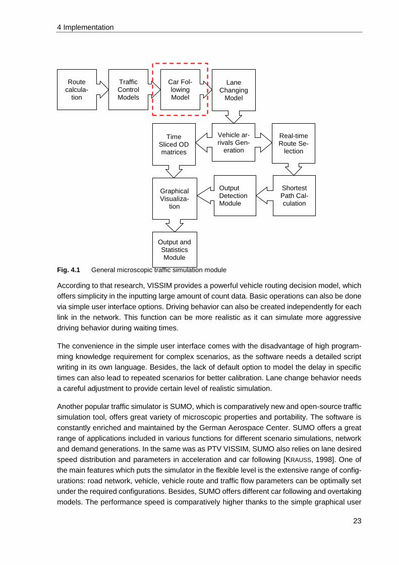
The general microscopic traffic simulation workflow in Fig. 4.1 is followed by many software
developers. One of the important modules is car following model, which the focus will be on.
One of the most popular discrete-time based microscopic models is VISSIM developed by PTV
Group. The simulator performs the traffic flow by moving the driver-vehicle units along the road
network.
By default, traffic dynamics is basically assigned by its longitudinal psychophysical car follow-
ing- model and latitudinal rule based lane changing model. Thanks to the flexibility in transport
planning and management, VISSIM has been widely used for research and commercial pur-
poses. SALGADO ET AL. [2016], compares the application of several micro traffic simulators for
general purposes.
4 Implementation
23
Fig. 4.1 General microscopic traffic simulation module
According to that research, VISSIM provides a powerful vehicle routing decision model, which
offers simplicity in the inputting large amount of count data. Basic operations can also be done
via simple user interface options. Driving behavior can also be created independently for each
link in the network. This function can be more realistic as it can simulate more aggressive
driving behavior during waiting times.
The convenience in the simple user interface comes with the disadvantage of high program-
ming knowledge requirement for complex scenarios, as the software needs a detailed script
writing in its own language. Besides, the lack of default option to model the delay in specific
times can also lead to repeated scenarios for better calibration. Lane change behavior needs
a careful adjustment to provide certain level of realistic simulation.
Another popular traffic simulator is SUMO, which is comparatively new and open-source traffic
simulation tool, offers great variety of microscopic properties and portability. The software is
constantly enriched and maintained by the German Aerospace Center. SUMO offers a great
range of applications included in various functions for different scenario simulations, network
and demand generations. In the same was as PTV VISSIM, SUMO also relies on lane desired
speed distribution and parameters in acceleration and car following [KRAUSS, 1998]. One of
the main features which puts the simulator in the flexible level is the extensive range of config-
urations: road network, vehicle, vehicle route and traffic flow parameters can be optimally set
under the required configurations. Besides, SUMO offers different car following and overtaking
models. The performance speed is comparatively higher thanks to the simple graphical user
Route calcula-
tion
Traffic Control Models
Car Fol-lowing Model
Lane Changing
Model
Shortest Path Cal-culation
Graphical Visualiza-
tion
Vehicle ar-rivals Gen-
eration
Real-time Route Se-
lection
Time Sliced OD matrices
Output Detection Module
Output and Statistics Module

4 Implementation
24
interface. For more complex scenarios and taking control over higher level simulations TraCI
interface can be used.
However, all counted advantages come with a slight number of shortcomings such as lane
traffic simulation which forces all the vehicle in the network to follow lane change rules. Nev-
ertheless, the data being used in this study is based on the one lane road with the restrictions
in changing, which should make it perfect to use for this purpose.
4.4.2 Options of data-driven model implementation into the simulator SUMO
As discussed in the previous section, SUMO is an open-source software which can be ex-
tended under specific needs and requirements depending on the purpose of the task. Besides,
several applications from independent developers and researchers exit as an open source
extension. Therefore, it is interesting to see all the options and choose the optimum one. Fur-
ther, three options will be discussed.
The DLR SUMO is written in C++ and the open source files for the compilation is available for
downloading on the official website of DLR. Once the necessary build version is downloaded,
it can be used for further applications. In the framework of the flexibility, SUMO offers creating
an own car following model and implementing it into the software. There is a detailed manual
on the steps how to apply it. However, by the new car following model, the software implies
collision avoidance models. In our specific case where the data-driven model is used, this
feature becomes useless.
In order to diminish this shortcoming, building a connection between the traffic simulator and
a flexible regression tool would be required.
As a flexible regression estimator, the statistical software R was chosen (C++ implementation
is called Rcpp [http://www.rcpp.org/]). Since Rcpp offers fast calculation, this would be a per-
fect choice, as the software should return the estimated values to the simulator on real-time.
As both software are open-source and written in C++, theoretically there should be no limita-
tions in successfully integrating them together. Moreover, the extended compiled version
would allow the comfortable environment for further changes to use different functions to esti-
mate the speed values.
According to the connection offered above, at the stage of vehicle behavior model in the seg-
ment of car following models, SUMO would address the Rcpp part, instead of doing conven-
tional speed estimation. Rcpp, in the same time would load the R script containing necessary
function as well as the observation data, thereby combining and simultaneously calculating the
estimated speed.

4 Implementation
25
Fig. 4.2 Extended SUMO after compilation with new data-driven model
However, according to the official website of the Rcpp developers, the package doesn’t support
the Visual Studio [dirk.eddelbuettel.com/code/rcpp/Rcpp-FAQ.pdf], whilst SUMO for Windows
version can be compiled only in Visual Studio [http://sumo.dlr.de/wiki/Installing/Win-
dows_Build].
As mentioned in the previous parts, SUMO offers extended control over the simulation process
as well as the parameters involved there. The software offers this variety options through the
interface called TraCI [WAGENER ET AL., 2008]. There is a detailed manual on how to use and
the command library of the software on the official website of the developer.
TraCI, builds a connection between the controller of the simulation process and the simulator
SUMO. It serves as a server to manipulate the simulation on-line.
According to this method, Python acts as a main controller over the whole process, as the
TraCI commands can be transmitted to SUMO only in python language. As the flexible regres-
sion calculator, still the statistical software R can be used. For Python implementation, there is
a library package called rpy2. For the test purpose, the R 3.3.2 version along with rpy2 - 0.2.8
build on WinPython 2.7.10.3 were used. As the versions are on continuous development, even
slight changes in the version can bring into malfunction of the system as there are two server
participants as TraCI and rpy2.
The process starts with the Python code creating an environment for running the simulation of
SUMO. Python sends the call function via TraCI to SUMO in order set the speed of the first
car in the network. After, via the same interface, Python code retrieves the speed of the leading
and following car as well as the distance between them. Then, it sends the acquired details to
R script via rpy2, from where it returns the estimated speed of the following car for the next
time step.

4 Implementation
26
Fig. 4.3 SUMO connection to R over Python
Despite the simplicity of the build connection, there are several shortcomings of the system.
First of all, the stability of the connection goes under question as there are two bridging libraries
and in case of the failure or access denial, the simulator will not follow. The key disadvantage
comes here in the performance of the model as the calculation speed. Even though Python
along with SUMO via TraCI has quite impressive speed, the rpy2 cannot provide the parallel
information exchange bandwidth as the former. Therefore, this connection mode can be ap-
plied only to the networks and trajectories where the number of vehicles doesn’t exceed the
number ten.
The limitations above led to try another way of pairing these two systems. The connection
explained in the Fig. 4.3, assigns the Python in the center as in the previous method, yet the
calculations are also done directly in the python code itself.
Python is popular for extensive and powerful libraries for great variety of tasks. For statistical
calculations, python uses library extension statistical models. Once the library loaded to the
system, it can be used as a native calculation tool. This adds flexibility, performance speed
and simplicity in using the extension. Smoothness of the simulation is guaranteed now.

4 Implementation
27
Fig. 4.4 SUMO with loaded flexible regression algorithms via Python
Taking an advantage of using the high-speed calculation possibilities, a better connection can
be created. After loading both calculation extension and observation data, Python addresses
and sets the necessary values to the given parameters.
4.5 Simulation specifications and setup
4.5.1 Design parameters
The quality of simulation process highly depends on setting the correct parameters and taking
into consideration the design features as well as those of simulators. Within the framework of
this study, several runs will be performed on three routes. For each data series, the corre-
sponding time interval will be chosen.
Every simulation software assumes the warmup period. This period begins immediately when
the simulation is executed and lasts till the all vehicle in the network are loaded. The same is
true for the speed which vehicles should be set. Therefore, the values manipulated within the
warmup period should be taken into consideration during the analysis.
The trajectory data series from Naples is based on the time steps of 10 ms and the same time
step can be provided by SUMO. PAPATHANASOPOULOU AND ANTONIOU [2015] provided a de-
tailed sensitivity analyses for the data driven model based on locally weighted regression
where she found the following parameters being the most justified: maximum desired acceler-
ation 𝛼𝑛 = 1.6 𝑚/𝑠2 , maximum desired deceleration𝑏𝑛 = 1.6 𝑚/𝑠2, maximum desired speed
𝑉𝑛 = 16 𝑚/𝑠, reaction time 𝜏 = 0.4 𝑠. Similarly, the same settings for the data-driven model will

4 Implementation
28
be applied. Regarding the Krauss model parameters, thorough sensitivity analysis will be pro-
vided in the next chapter.
Regarding the Naples network, the map was retrieved from www.openstreetmap.org and
adapted under the simulation circumstances. These include, conversion of simple edge-node
roads into polyline links to provide more realistic performance of the simulations, as vice versa,
the vehicles in the network could recognize the nodes as the possibility to have a turning point.
To create the trips, a unified python code was implemented, according to which the number of
vehicles in the network can be manipulated by entering the necessary value.
4.5.2 Naples Network
The data-collection observations were performed in the Naples Metropolitan, where three cor-
ridors were chosen. A detailed description of the experiment data can be found in the study by
PUNZO ET AL. [2005]. The exact replica of the roads was modeled using the standard tools of
SUMO for network generation.
Four vehicles moved in the same platoon and in the same sequence, where the first vehicle
served as a leader and the rest three as the followers. However, driving session differentiated
as well as the route and traffic conditions. The data series A, includes two segments of car
following state, one lasting for 35.8 s, and the second 17.2 s (named as A358 and A172 cor-
respondingly).
Fig. 4.5 SUMO representation of Naples network for data series A.

4 Implementation
29
This data series belongs to urban area and have one lane per direction. The data series takes
the start from Piazza Gabriele D’Annunzio in the south and along Cupo Nuova Cintia attaches
to the street Viale Traiano in the north. This data series belongs to urban area and have one
lane per direction.
Fig. 4.6 SUMO representation of Naples network for data series B.
The longest data series from the Naples observations is B series which provides continuous
car following state for 169.5 s (named as B1695). The vehicles start their movement from the
highway of Via Solfatara and following to Variante Solfatara branch, moving from east to north-
west.
It should be considered, that the road crosses the suburban area. Trajectory data retrieved
from the data series B, was also used for the model calibration. The rest five series were used
for validating. The speed ranged from 0.11 m/s to 19.00 m/s, with the mean of 12.18 m/s.
The last data series include three segments with durations of 62.1s, 16.8s and 17.1s (named
as C621, C168 and C171 respectively) correspondingly. The road topography is straight and
starting from the south west stretches to the north-east along the street Via Terracina with the
total length of 1.8 km.
Despite the fact that the topology of the road network in this data series is quite straight, it can
provide with the different speed deviations, as the speed ranges from 0.1 m/s up to 13.22 m/s.

4 Implementation
30
Fig. 4.7 SUMO representation of Naples network for data series C.
4.5.3 Algorithm and procedure explanation
The basic principle according to which the connection works is as following: Python controller
creates an environment for performing all the necessary calculations. This data series belongs
to urban area and have one lane per direction. Next, the flexible regression module is included
as well as the necessary data series, Python controller performs the fitting. Then, the road
network is loaded to the environment and immediately forwarded to SUMO. It is important to
mention that interactions with SUMO is provided via TraCI, which acts as a server. After the
road network import, the trip information is generated. For that purpose, another file is created
in order to run the complete SUMO configuration.
To provide flexibility, a separate file writing is done in the Python environment, allowing to
easily change the number of vehicles and their type. Then, data regarding time steps and
parameters are set and send to SUMO. These parameters include the speed of the leading
car too. Then, the triples of the speeds for two vehicles and the gap between them is retrieved
and applied to the flexible regression model. Finally, the estimated following speed is send
back to SUMO to setting to the necessary vehicle. Below, the algorithm of the procedure is
provided for better understanding.

4 Implementation
31
Fig. 4.8 Python and SUMO interaction algorithm
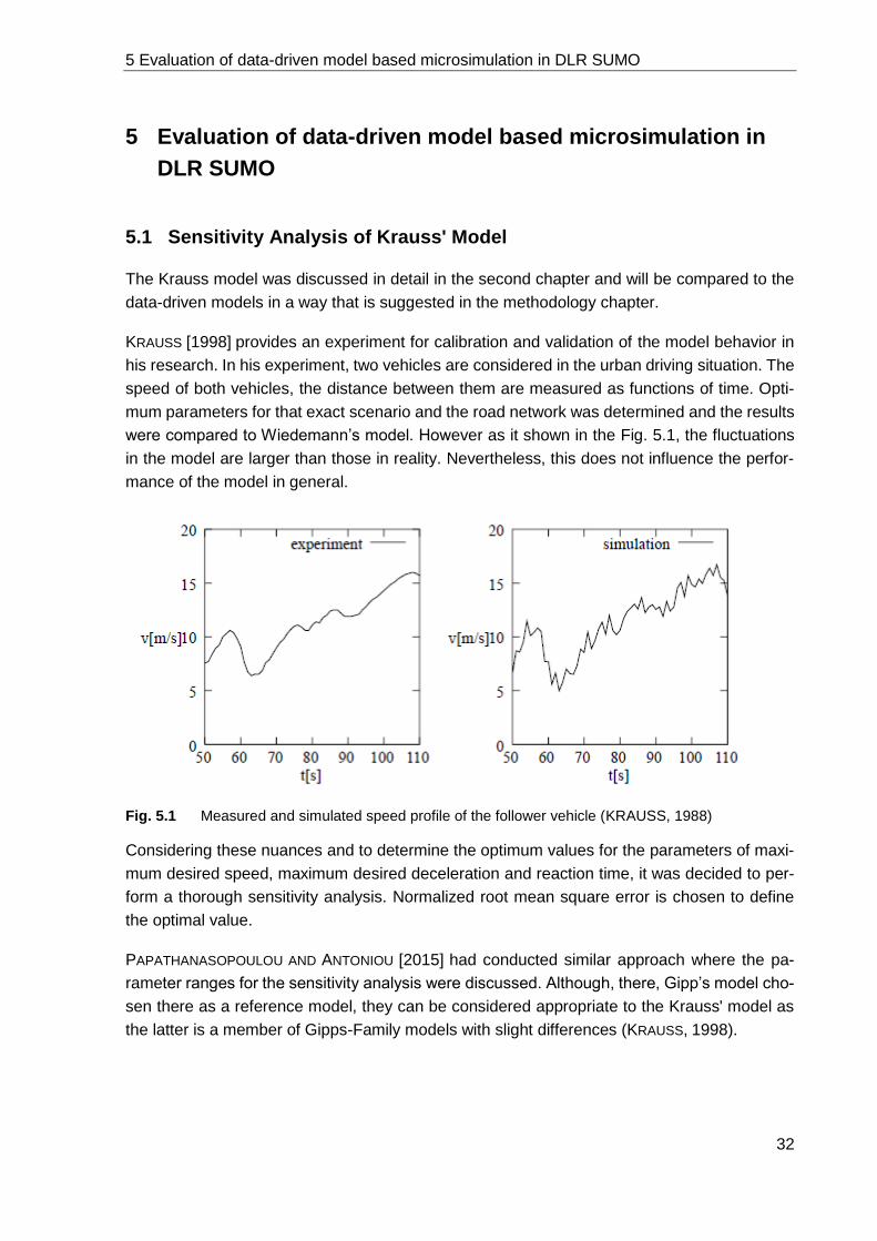
5 Evaluation of data-driven model based microsimulation in DLR SUMO
32
5 Evaluation of data-driven model based microsimulation in
DLR SUMO
5.1 Sensitivity Analysis of Krauss' Model
The Krauss model was discussed in detail in the second chapter and will be compared to the
data-driven models in a way that is suggested in the methodology chapter.
KRAUSS [1998] provides an experiment for calibration and validation of the model behavior in
his research. In his experiment, two vehicles are considered in the urban driving situation. The
speed of both vehicles, the distance between them are measured as functions of time. Opti-
mum parameters for that exact scenario and the road network was determined and the results
were compared to Wiedemann’s model. However as it shown in the Fig. 5.1, the fluctuations
in the model are larger than those in reality. Nevertheless, this does not influence the perfor-
mance of the model in general.
Fig. 5.1 Measured and simulated speed profile of the follower vehicle (KRAUSS, 1988)
Considering these nuances and to determine the optimum values for the parameters of maxi-
mum desired speed, maximum desired deceleration and reaction time, it was decided to per-
form a thorough sensitivity analysis. Normalized root mean square error is chosen to define
the optimal value.
PAPATHANASOPOULOU AND ANTONIOU [2015] had conducted similar approach where the pa-
rameter ranges for the sensitivity analysis were discussed. Although, there, Gipp’s model cho-
sen there as a reference model, they can be considered appropriate to the Krauss' model as
the latter is a member of Gipps-Family models with slight differences (KRAUSS, 1998).

5 Evaluation of data-driven model based microsimulation in DLR SUMO
33
The suggested parameter ranges based on GIPPS [1981] and RANJITKAR ET AL. [2005], are
illustrated in the Fig. 5.2. When it comes to the reaction time suggestions, even more refer-
ences were used (Fig. 5.3):
Fig. 5.2 Range of parameters according to references [PAPATHANASOPOULOU AND ANTONIOU, 2015]
Fig. 5.3 Range of reaction time according to references [PAPATHANASOPOULOU AND ANTONIOU, 2015]
The results were as following: reaction time 𝜏: 0.4 − 3.0 𝑠, maximum desired speed 𝑉𝑛: 10.4 −
29.6 𝑚/𝑠, maximum desired deceleration 𝑏𝑛: 1.6 − 5.2 𝑚/𝑠2.
For the sensitivity analysis of the Krauss' model, the data series C171 was chosen. The opti-
mum combination of parameter values was performed for entire trajectory. The least overall
error based on normalized root mean square was considered as optimum.

5 Evaluation of data-driven model based microsimulation in DLR SUMO
34
Fig. 5.4 Sensitivity analysis for parameters of Krauss' model
As it can be seen from the Fig. 5.4, the overall error increased with the increase in reaction
time, while the maximum desired deceleration had a contrariwise effect. As a result, the best
performance of Krauss' model was achieved with the combination of following parameters: 𝜏 =
0.4 𝑠, 𝑉𝑛 = 15𝑚/𝑠, 𝑏𝑛 = 5.3 𝑚/𝑠2.
To increase the performance speed, the procedure for sensitivity analysis was performed in
Python version 2.7.10.3 using the own script. As shown in Fig. 5.5, a loop containing the pa-
rameters with values and the steps of 0.1are inputted. Then for each simulation SUMO simu-
lation was executed without using the graphical user interface to increase the simulation
speed. The warmup periods of the simulator were considered during the NRMSE analysis.
After the set of simulations were conducted, the outputs were analyzed and plotted in the sta-
tistical software R.
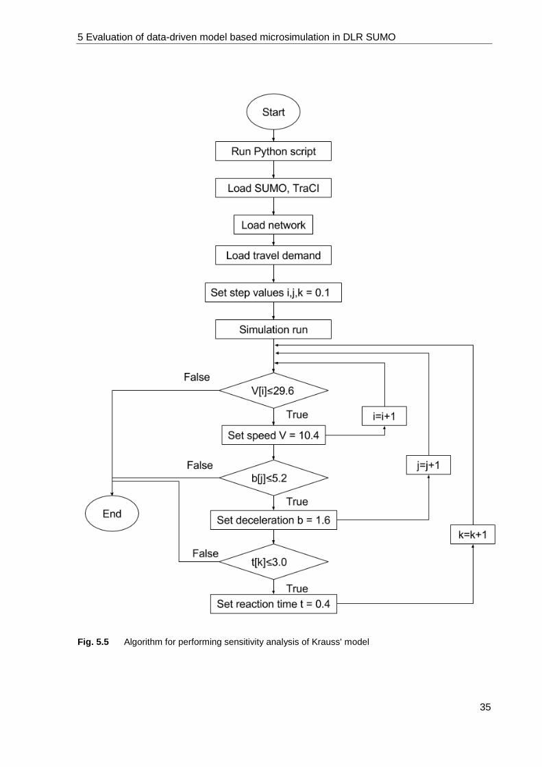
5 Evaluation of data-driven model based microsimulation in DLR SUMO
35
Fig. 5.5 Algorithm for performing sensitivity analysis of Krauss' model

5 Evaluation of data-driven model based microsimulation in DLR SUMO
36
5.2 Application of flexible regression
Both flexible regression models were implemented into SUMO via Python libraries. To fit the
data as good as possible, locally weighted regression needs optimum values for the span (𝛼)
and degree. The span varies from 0 to 1 and indicates the smoothness of the curve, while
degree indicates the degree of local polynomials in the regression. Kernel regression lacks the
manipulator such as degree and uses the parameter bandwidth the same as in loess to control
the smoothness [BREHENY, 2012]. The degree of the local polynomials defines the function:
the value 1 sets to linear function and 2 to quadratic.
PAPATHANASOPOULOU AND ANTONIOU [2015] in the similar research, provided detailed sensitiv-
ity analysis for the loess application. Fig. 5.6 and Fig. 5.7 shows the influence of the degree
and span on overall error as well as the selected span ranges correspondingly. As the sensi-
tivity analysis was performed on the same trajectory data using the same flexible regression
technique, the optimum parameters from that research will be used. It is necessary to highlight
that the both loess and kernel regression, as well as Krauss' model used the speeds of the
second and the third vehicles (𝑣2, 𝑣3) as well as the distance between them (𝐷23) to ensure the
reasonability of comparison. PAPATHANASOPOULOU AND ANTONIOU [2015] discovered that out
of all follower-leader combinations B1695 series had the best performance of flexible regres-
sion.
Fig. 5.6 NRMSE for different values of span and degree, by applying the method loess for a reaction
time s = 0.4 s [PAPATHANASOPOULOU AND ANTONIOU, 2015]

5 Evaluation of data-driven model based microsimulation in DLR SUMO
37
Fig. 5.7 Ranges of span to minimize the NRMSE for each data series [PAPATHANASOPOULOU AND
ANTONIOU, 2015]
The same series was used in this thesis for the rest of the data series. Additionally, one of the
key aspects in implementing the flexible regression method is the reaction time. The reaction
time influences the results of application of flexible regression method, due to the fact that for
various values of reaction time 𝑠 data with different time instants are selected for speed pre-
diction. In case the prediction for time instant 𝑡 is needed, then data for time instant (𝑡 − 𝜏) are
applied. Further, the paper discusses that, the same values of reaction time as those used for
Gipps’ calibration were used, to provide a reasonable comparison.
Fig. 5.6 shows the impact of degree to the overall error, where the dashed lines demonstrate
the NRMSE of speed 𝑣3(𝑡 + 𝜏)estimation with loess method. There, degree equaling 1 for each
data series and for each value of span among its range were considered, while the solid lines
indicate the corresponding results for degree of 2. The dashed lines look smoother and illus-
trate lower NRMSE than solid lines, which resulted choosing the degree 1 as an optimum.
Coming to the span, the dashed lines show less influence for values of span between 0.4 and
1.0 for all data sets. To conclude, except low values, the span does not impact noticeably the
results. Additionally, the ranges of the span, for which observed the lowest NRMSE for each
data series, are designated in Fig. 5.7. By default, the value 0.75 is chosen as an average.
5.3 Validation and results
The performance of speed estimation of the third vehicle 𝑣3(𝑡 + 𝜏)for three cases: Krauss’
model, data-driven model based on locally weighted regression and kernel regression are
shown in the Fig. 5.8. In all data series, both kernel regression and loess showed much accu-
rate results compared to the reference model. It is clear from the Fig. 5.9, that the RMSPE
shows the large error more heavily as compared to the previous goodness-of-fit method.

5 Evaluation of data-driven model based microsimulation in DLR SUMO
38
Fig. 5.8 Normalized root mean square error for all data series
Fig. 5.9 Root mean square percentage error for all data series
MPE shows the under and overestimations in the output of six data series. Regarding the
Theil’s inequality coefficient U, both flexible regression models were close to perfect fit as com-
pared to the Krauss’ model. In the data series C, the fit was comparatively inferior due to the
difference in road network topology and the data series used for calibration.
In some data series, the Theil’s 𝑈𝑠 coefficient (Fig. 5.12) showed comparatively higher values.
This means that the model replicated more the variability in the observed data.

5 Evaluation of data-driven model based microsimulation in DLR SUMO
39
Fig. 5.10 Mean percentage error for all data series
Fig. 5.11 Theil’s inequality coefficient 𝑈 (top) and 𝑈𝑚(bottom) for all data series

5 Evaluation of data-driven model based microsimulation in DLR SUMO
40
Fig. 5.12 Theil’s inequality coefficients 𝑈𝑠for all data series
The predicted data showed more similar to the free flow speed which was caused by quite low
standard deviation compared to the observed data.
Fig. 5.13 Normality and homoscedasticity plot of kernel (left) and loess (right) techniques
In addition to the goodness-of-fit analysis, the produced residuals analysis is also performed.
This was done to reveal bias in the estimation of speed by testing the assumptions of normality,

5 Evaluation of data-driven model based microsimulation in DLR SUMO
41
linearity and homoscedasticity. The plot of standardized residuals versus standardized pre-
dicted values was used to indicate the linearity and homoscedasticity. The normality was tested
using normal quantile plots.
The plot of standardized residuals versus standardized predicted values is concentrated along
the horizontal line, thereby submitting the assumptions. In the same way, normal quantile plot
(Q - Q) is considered sufficient, as the deviations are almost along the diagonal line. To con-
clude, no bias in estimation of speeds were found.

6 Conclusion
42
6 Conclusion
6.1 Summary
In the current thesis, two flexible regression techniques were implemented to the microscopic
traffic simulator SUMO and validated with several data series for plausibility. One of the flexible
regression techniques is locally weighted regression and the other is kernel regression. Both
were used to predict the speed of the following vehicle in a car following state.
The thesis began with a review of the corresponding topic. First, it was determined that flexible
regression models have benefits over the widely used traditional safety distance models. Later,
Krauss’ model was chosen as a reference model to the proposed flexible regression models,
since it has relatively higher accuracy in the corresponding microscopic traffic simulator. After
the discussion of the traditional models, it was decided to implement a data-driven model to
the chosen simulator for further possibility validation of this approach at network level. Main
reason is the data-driven models have a noticeable advantage of speed predictions and can
be applied thanks to the high computational capabilities of current computers. Another reason
is the existence of successful implementation results.
In order to perform the estimation of flexible regression, the appropriate software was chosen.
Then, several options of application were reviewed. After the optimum way of implementing
was introduced: Python and SUMO, which is the core of this thesis.
After that, several simulations were performed at the same experiment network to evaluate the
quality of proposed methodology. The following are the main findings regarding the perfor-
mance and efficiency of the data-driven methods:
First, the outcomes of both regression techniques are quite promising. They demonstrated that
the performance of both loess and kernel regression techniques outperform that of Krauss’s
model in all data series. Both regressions provide higher level of speed prediction smoothly
even in the simulator environment. These advantages become more evident in the data series
with complex trajectory. However, the discrepancy between reference and proposed model
reduces when the trajectory of the data is straighter.
Secondly, the results show that the locally weighted regression is even more accurate in pre-
dictions compared to the kernel regression technique. Except the slight inaccuracy in one of
the data series, loess outperforms both models.
Thirdly, by changing the values of selected three parameters in the sensitivity analysis of
Krauss’ model, the optimum values were proved. The results for sensitivity analysis were sim-
ilar to the findings of the previous work due to the similar car following model approach. Taking
into consideration of previous researches towards the similar topic, sensitivity analysis for the

6 Conclusion
43
flexible regression models were omitted. As the optimum values for the span and degree were
determined for the same data series, they were chosen for the implementation.
Lastly, the speed estimations were checked for bias for all data series. The results were suffi-
cient as the assumptions on normality and homoscedastic were met. In details, the deviations
of the normality check plot along the diagonal line in the center plot were close to minimum,
although it differentiated at both ends, showing a slight tail in both ends. As the values of
standardized predicted values were built up across the horizontal line, the lack of bias was
approved.
6.2 Outlook
The data-driven approach implemented in this thesis have been suggested that they can
achieve a better performance than the traditional car following model such as Krauss’s. The
generalized data-driven car following model implemented in SUMO, was validated for perfor-
mance using the available trajectory data which was based on a single lane road. Therefore,
different direction exists for future researches in this topic. The following are proposed for po-
tential improvements regarding the data-driven models and their validation.
First, the model used for simulation in this research assumes a single lane road network. The
lateral movement of a vehicle and interacting with other vehicles by lanes should be studied.
In addition to this, the behavior should be tested in the situations where the vehicle interacts
with road curvatures, traffic lights at intersections etc. [PAPATHANASOPOULOU AND ANTONIOU,
2015].
Secondly, factors such as road type [BRACKSTONE, 2009] driver’s characteristics such as age,
reaction time, experience and other factors influencing the driver’s behavior should be studied
further.
Finally, data such as vehicle type in the simulation and surrounding area should also be applied
as variables to estimate the speed.
Despite the provided successful results from the implementation of data-driven models, tradi-
tional safety distance based car following models such as Krauss’s, demonstrate better insight
to overall traffic flow theory.

7 List of References
44
7 List of References
ANTONIOU C.; BALAKRISHNA R.;KOUTSOPOULOS H. [2011]: A synthesis of emerging data collec-
tion technologies and their impact on traffic management applications. Eur. Transp. Res.
Rev. 3 (3), 139–148. http://dx.doi.org/10.1007/s12544-011-0058-1.
ANTONIOU C.; GIKAS V.; PAPATHANASOPOULOU V.; MPIMIS T.; MARKOU I.; PERAKIS H.; [2014]:
Towards distribution-based calibration for traffic simulation. In: 17th International IEEE
Conference on Intelligent Transportation Systems, Qingdao, China, October 8–11, pp.
780–785.
ANTONIOU C.; KOUTSOPOULOS H. [2006]: Estimation of traffic dynamics models with machine
learning methods. Transp. Res. Rec.: J. Transp. Res. Board 1965, 103–111 (Washing-
ton, DC).
ANTONIOU C.; KOUTSOPOULOS H.; YANNIS G.; [2013]: Dynamic data-driven local traffic state
estimation and prediction. Transp. Res. Part C: Emerg. Technol. 34, 89–107.
ARON M.; [1988]. Car following in an urban network: simulation and experiments. In Proceed-
ings of Seminar D, 16th PTRC Meeting (pp. 27-29)
BARTHAUER M.; FRIEDRICH B.; [2016]: Calibrating a Motorway Segment in SUMO Using Single
Vehicle Data. Proceedings of the SUMO2016, Berlin, 2016 pp. 11-13
BIFULCO G.N.; PARIOTA L.; SIMONELLI F.; DI PACE R.; [2013]: Development and testing of a fully
Adaptive Cruise Control system. Transp. Res. Part C 29 (2013), 156–170.
BRACKSTONE M.; MCDONALD M.; [1999]: Car-following: a historical review. Transp. Res. Part F
2 (4), 181–196.
BRACKSTONE M.; WATERSON B.; MCDONALD M.; [2009]: Determinants of following headway in
congested traffic. Transp. Res. Part F: Traffic Psychol. Behav. 12 (2), 131–142.
BRACKSTONE, M.; MCDONALD M.; [1999]: Car-following: a historical review. Transp. Res. Part
F 2 (4), 181–196.
BREHENY P. [2012]: Nonparametric Statistics, pp-3-23
CHENG B.; TITTERINGTON D.; [1994]: Neural networks: a review from a statistical perspective.
Statistical Science 9, 2–54.
CLEVELAND W.S.; [1979]: Robust locally weighted regression and smoothing scatterplots. J.
Am. Stat. Assoc. 74 (1978), 829–836.

7 List of References
45
DOWLING. R.; SKABARDONIS A.; HALKIAS J.; HALE G.; ZAMMIT G.; [2004]: Guidelines for calibra-
tion of microsimulation models: framework and applications. Transport. Res. Rec. J.
Transport. Res. Board 1876, 1–9.
EVANS, L.; ROTHERY, R. [1973]. Experimental measurement of perceptual thresholds in car fol-
lowing. Highway Research Record, 64, 13-29.
GIPPS, P.G.; [1981]: A behavioral car following model for computer simulation. Transp. Res.
Part B 15, 105–111.
HANKEN, A.; ROCKWELL, T.H. [1967]: A model of car following derived empiriacally by piece-
wise regression analysis.In Proceedings of the 3rd International Symposium on the The-
ory of Traffic Flow (pp. 40-41). New York: Elsevier.
HELLY, W., [1961]: Simulation of bottlenecks in single lane traffic flow. In: Theory of Traffic
Flow, Elsevier Publishing Co., pp. 207–238.
JEONG, R., RILETT, L.R., [2005]: Bus arrival time prediction model for real-time applications.
Transportation Research Record 1927, 195–204.
KARLAFTIS M.; VLAHOGIANNI E.; [2011]: Statistical methods versus neural networks in transpor-
tation research:Differences, similarities and some insights. Transportation Research Part
C 19 (2011) 387–399
KIKUCHI C.; CHAKROBORTY P.; [1992]: Car following model based on a fuzzy inference system.
Transp. Res. Rec. 1365, 82–91.
KOMETANI, E.; SASAKI, T; [1958]: On the stability of traffic flow. Report no. 1. J. Oper. Res. Jpn.
2 (1), 11–26.
KOUTSOPOULOS, N.; FARAH, H.; [2012]: Latent class model for car following behavior. Transp.
Res. Part B 46 (2012), 563–578.
KRAJZEWICZ D.; JAKOB ERDMANN J.; BEHRISCH M.; BIEKER L.; [2012]: Recent Development and
Applications of SUMO – Simulation of Urban Mobility. International Journal on Advances
in Systems and Measurements, vol 5 no 3 & 4, year 2012, pp 128-138.
KRAUSS S.;[1998]: Microscopic Modeling of Traffic Flow: Investigation of Collision Free Vehicle
Dynamics. Dissertation, Cologne 1998.
LEUTHOLD R.;[1975]: On the use of Theil’s inequality coefficient. Americal Journal of Agroeco-
nomics, (1975) 57 (2): 344-346.
LEUTZBACH, W.; [1988]: Introduction to the Theory of Traffic Flow. Springer Verlag, Berlin.
LIU R.; LI X.; [2013]: Stability analysis of a multi-phase car-following model. Physica A: Stat.
Mech. Appl. 392 (11), 2660–2671.

7 List of References
46
NADARAYA E.; [1964] On estimating regression, Theory of probability and its applications, 9(1),
141-142.
OLSTAM, J.J.; TAPANI, A.; [2004]. Comparison of Car-following Models. Swedish National Road
and Transport Research Institute, VTI Meddelande 960A & #xB7.
PANWAI S., DIA H.; [2007]: Neural agent car-following models. IEEE Transactions on Intelligent
Transportation Systems 8 (1), 60-70
PAPATHANASOPOULOU V.; ANTONIOU C. [2015]: Towards data-driven car-following models.
Transportation Research Part C 55 (2015) 496–509
PAPATHANASOPOULOU V.; ANTONIOU C. [2017]: A comparison of machine learning techniques
for data–driven car–following models. Transportation Research Procedia 00 (2016) 000–
000
PUNZO, V.; FORMISANO, D.J.; TORRIERI, V.; [2005]: Part 1: traffic flow theory and car following:
nonstationary Kalman filter for estimation of accurate and consistent car-following data.
Transp. Res. Rec.: J. Transp. Res. Board 1934 (1), 1–12.
RANJITKAR, P., SUZUKI, H., NAKATSUJI, T., [2005]: Microscopic traffic data with real-time kine-
matic global positioning system. In: Proceedings of Annual Meeting of Infrastructure
Planning and Management, Japan Society of Civil Engineer, Miyazaki, Preprint CD, De-
cember 2005.
SALGADO D.; JOLOVIC D., MARTIN P., ALDRETE R; [2016]: Traffic Microsimulation Models As-
sessment – A Case Study of International Land Port of Entry, The 7th International Con-
ference on Ambient Systems, Networks and Technologies (ANT 2016) /The 6th Interna-
tional Conference on Sustainable Energy Information Technology (SEIT-2016) /Affiliated
Workshops, Procedia Computer Science, 83 (2016) 441-448.
SARLE, W.; [1994]. Neural networks and statistical models. In: Proceedings of the Nineteenth
Annual SAS Users Group International Conference (April 1–13).
SIMONELLI, F., BIFULCO, G.N., DE MARTINIS, V., PUNZO, V., [2009]. Human-like adaptive cruise
control systems through a learning machine approach. In: Applications of Soft Compu-
ting. Springer, Berlin, Heidelberg, pp. 240–249.
SMITH S.; SINCICH T.;[1988] Stability over time in the distribution of population forecasts errors.
Demography. 1988; 25:461–474. doi: 10.2307/2061544
THEIL, H., [1978]. Introduction to Econometrics. Prentice Hall, New Jersey.
TORDEUX, A., LASSARRE, S., ROUSSIGNOL, M., [2010]: An adaptive time gap car-following
model. Transp. Res. Part B 44 (8–9), 1115–1131.

7 List of References
47
TREIBER, M., HENNECKE, A., HELBING, D., [2000]: Congested traffic states in empirical observa-
tions and microscopic simulations. Phys. Rev. E 62 (2), 1805.
VLAHOGIANNI, E.I., KARLAFTIS, M.G., GOLIAS, J.C., [2005]: Optimized and meta-optimized neu-
ral networks for short-term traffic flow prediction: a genetic approach. Transp. Res. C 13
(3), 211–234.
WEGENER A.; PIORKOWSKI M.; RAYA M.; HELLBRACK H.; FISCHER S; HUBAUX J.;[2008]: TraCI:
An Interface for Coupling Road Traffic and Network Simulators. The 11th Communica-
tions and Networking Simulation Symposium CNS'08, Ottawa (Canada)
ZHANG, H.M., KIM, T., [2005]. A car-following theory for multiphase vehicular traffic flow. Transp.
Res. Part B 39, 385–399.

8 List of Abbreviations
48
8 List of Abbreviations
CI Computational Intelligence
DLR Deutsches Zentrum für Luft- und Raumfahrt
LOESS Locally weighted regression
MPE Mean Percentage Error
NN Neural networks
NRSME Normalized Root Mean Square Error
RMSPE Root Mean Square Percentage Error
SUMO Simulator of Mobility
TraCI Traffic Control Interface
VISSIM Verkehr In Städten - SImulationsModell

9 List of Symbols
49
9 List of Symbols
𝑣𝑠𝑎𝑓𝑒 [𝑚
𝑠] Safety speed of the vehicle
𝑣𝑑𝑒𝑠 [𝑚
𝑠] Desired maximum speed of the vehicle
𝜏 [𝑠] Reaction time
𝑔𝑑𝑒𝑠 [𝑚] Desired gap
𝑏𝑛 [𝑚/𝑠2] Maximum desired deceleration

10 List of Figures
50
10 List of Figures
Fig. 3.1 Methodological framework .....................................................................................................9
Fig. 3.2 Sensitivity analysis and selection of parameters’ optimum values ..................................... 11
Fig. 4.1 General microscopic traffic simulation module ................................................................... 23
Fig. 4.2 Extended SUMO after compilation with new data-driven model ........................................ 25
Fig. 4.3 SUMO connection to R over Python ................................................................................... 26
Fig. 4.4 SUMO with loaded flexible regression algorithms via Python ............................................ 27
Fig. 4.5 SUMO representation of Naples network for data series A. ............................................... 28
Fig. 4.6 SUMO representation of Naples network for data series B. ............................................... 29
Fig. 4.7 SUMO representation of Naples network for data series C. ............................................... 30
Fig. 4.8 Python and SUMO interaction algorithm ............................................................................ 31
Fig. 5.1 Measured and simulated speed profile of the follower vehicle (KRAUSS, 1988)............... 32
Fig. 5.2 Range of parameters according to references (PAPATHANASOPOULOU AND
ANTONIOU, 2015) .............................................................................................................. 33
Fig. 5.3 Range of reaction time according to references (PAPATHANASOPOULOU AND
ANTONIOU, 2015) .............................................................................................................. 33
Fig. 5.4 Sensitivity analysis for parameters of Krauss' model ......................................................... 34
Fig. 5.5 Algorithm for performing sensitivity analysis of Krauss' model ........................................... 35
Fig. 5.6 NRMSE for different values of span and degree, by applying the method loess for a
reaction time s = 0.4 s (PAPATHANASOPOULOU AND ANTONIOU, 2015) .................... 36
Fig. 5.7 Ranges of span to minimize the NRMSE for each data series (PAPATHANASOPOULOU
AND ANTONIOU, 2015) ..................................................................................................... 37
Fig. 5.8 Normalized root mean square error for all data series ....................................................... 38
Fig. 5.9 Root mean square percentage error for all data series ...................................................... 38
Fig. 5.10 Mean percentage error for all data series ........................................................................... 39
Fig. 5.11 Theil’s inequality coefficient 𝑈 (top) and 𝑈𝑚(bottom) for all data series ............................ 39
Fig. 5.12 Theil’s inequality coefficients 𝑈𝑠for all data series ............................................................. 40
Fig. 5.13 Normality and homoscedasticity plot of kernel (left) and loess (right) techniques.............. 40

11 Appendix A: Goodness-of-fit-outputs from all data series
51
11 Appendix A: Goodness-of-fit-outputs from all data series
Data Ser. A172 A358
Method Krauss Loess Kernel Krauss Loess Kernel
RMSN 0,067869 0,03276 0,03664 0,04763 0,02666 0,02638
RMSPE 0,06961 0,03192 0,03627 0,06275 0,0347 0,0346
MPE 0,069023 -0,0023 0,01705 0,04801 -0,01 0,00853
U 0,03257 0,01626 0,01802 0,0219 0,01252 0,01231
Um 1 0,00534 0,20489 0,71647 0,09506 0,07604
Us 1,16E-10 0,00632 0,00506 0,00373 0,01191 0,01216
Uc 3,07E-09 0,99433 0,79484 0,28061 0,8956 0,91442
Data Ser. B1695 C168
Method Krauss Loess Kernel Krauss Loess Kernel
RMSN 0,042204 0,02459 0,02682 0,03909 0,02087 0,02351
RMSPE 0,335821 0,14788 0,18379 0,03945 0,02085 0,02362
MPE 0,079357 0,01564 0,03077 0,03337 0,00198 0,01115
U 0,01984 0,01172 0,01274 0,01919 0,0104 0,01167
Um 0,67124 0,03179 0,18561 0,71737 0,00776 0,21826
Us 2,70E-05 ####### ####### 0,00121 0,00424 0,00334
Uc 0,328928 0,96871 0,8148 0,28317 0,99412 0,78323
Data Ser. C171 C621
Method Krauss Loess Kernel Krauss Loess Kernel
RMSN 0,098373 0,07476 0,07466 0,09437 0,06222 0,06887
RMSPE 0,132038 0,09231 0,09855 0,51309 0,22079 0,31048
MPE 0,081034 -0,0088 0,02403 0,15179 0,03127 0,07178
U 0,045396 0,03577 0,03525 0,04234 0,02864 0,03143
Um 0,445694 0,04035 0,03765 0,57947 0,03238 0,21029
Us 0,007379 0,01278 0,01281 0,0002 0,00046 0,00037
Uc 0,550286 0,95269 0,95537 0,42102 0,96874 0,79062

12 Declaration concerning the Master’s Thesis
52
12 Declaration concerning the Master’s Thesis
I hereby confirm that the presented thesis work has been done independently and us-
ing only the sources and resources as are listed. This thesis has not previously been
submitted elsewhere for purposes of assessment.
Munich, June 16th, 2017
_________________________
Muzaffar Khamraev