Markov-switching correlation models for contagion analysis in commodity and stock markets

Relatore : prof. Roberto Casarin

Studente : Azzedine Dridi

Università degli studi Ca' Foscari di Venezia

1) Introduction :

Commodity securities such as oil and gold have been subject to an increasing interest within this

period of Great Depression followed by the EU Sovereign Debt crisis, being for instance an extremely

popular investment class as part of a long-term diversification strategy (LTDS), offered by fund

managers. In the meanwhile there is little evidence of a lasting impact of financial investment on

commodity prices (see Fattouh et Al. 2012 for a recent survey). This leads to considering trading

motive of non-commercial financial investors as "noise-trading"- according to the microstructural

framework- based on systemic risk perception rather than idiosyncratic and market-specific

considerations. Hence, a large literature investigated correlation dynamics between equity and

commodities market variations during the last decade, extending the multivariate GARCH model

frameworks or multivariate stochastic volatility models to better capture the structure of time-

dependence between the investment classes. Notably we underline here: Killian and Park (2009)

show that equity-price reaction to oil price shocks were depending on their nature; Cassassus and

Higuera (2011) showing that oil-prices are good predictors of equity prices; Chang et al. (2011)

showing evidence of volatility spillovers between the two markets, i.e. only volatility changes and

spreads out across markets .

With this respect, Lombardi and Ravazzolo (2012) offer an original contribution to this literature by

investigating oil-equity prices co-movements to improve forecasts either direction using a

parsimonious constant parameter Bayesian framework and deriving a Bayesian dynamic conditional

correlation model. The model can capture the shift observed after 2008 (see Della Corte and

al.,2010) and over-performs a no-change random walk model when conducting density forecast (see

Lombardi and Ravazzolo, 2012). This gain permits a better portfolio management framework

incompounding commodity prices as a new class of assets. Joint-modeling is shown to generate

better profitability "relatively to constant parameter models and passive strategies, especially in

times of large swings" . Improving the gains of standard DCC GARCH, with a parsimonious , stable

and efficient model and suitable Bayesian inference, which allows for an easy-to-handle active

Portfolio Management tool.

This paper builds on a simplified version of the Markov-Switching correlation model offered by

Casarin, Tronzano, and Sartore (2013) .Hence we extend here the oil-equity market linkage paper

based on dynamical correlation by applying a two-redeem state Markov-Switching model to account

for shifts in correlations and allow a more stable portfolio management.

In fact contagion would imply serious issues on diversification, leading to underestimate global risk,

and thus the related possible loss, especially while computing Value at Risk and Expected Shortfall.

We apply on this purpose, following Casarin and al. (2013), a multivariate stochastic correlation

model where the parameters of the correlation dynamics and those of the log-volatility process are

driven by a single latent Markov chain (MS-DC-MSV). It has this advantage to assume independent

innovation process for the mean returns and Variance-Covariance matrix, which is in a way closer to

empirical findings by allowing independent exogenous shocks.

We follow then a suitable Bayesian inference procedure, based on MCMC estimation algorithm, to

both parameters, covariances and correlation dynamics. We can point out that Bayesian inference

allows to account of higher moments than the only mean-variance.

We report some of the outputs, especially estimated time-varying stochastic correlations and

volatilities. We will end by commenting on possible empirical evidence of contagion effect (contagion

as defined above).

2. Theoretical part :

2.1. Introduction :

We introduce Markov Switching stochastic correlation with two redeem states (low volatility, high

volatility) to model the time-varying volatility and correlation . This modeling is built on a simplified

version of the Bayesian Markov-Switching DC-MSV model applied in Casarin and Al. (2013).

Both the Dynamical Correlation Model offered by Engle (2002) as extension of the Constant

conditional correlation model of Bollerslev, and MSV type modeling account for time-varying

correlation structure, consistently with the empirical evidence related to financial time-series stylized

facts.

First we will briefly introduce the DCC-GARCH to get an intuition on the model used for the empirical

part of the paper, also because it has been subject to a very large literature and extensions. This type

of modeling is very popular for its parsimonious modeling and competitive results with respect to its

previous ARCH and VEC type models. For a survey on Multivariate GARCH models one can refer to

Bauwens and al. (2006).

Then we specify the model MS-DC-MSV , which is in direct line with a recent approach, modeling

time-varying and stochastic correlation structure using multivariate SV models. Casarin et al. refers

for this approach to Gourieroux et al. (2004) on the one hand, on the other on Philipov and Glickman

(2006) , and Asai and McAleer (2009) on the other. To this purpose ,they assume that the covariance

matrix is a function of a Wishart process, which introduces stochastic behavior in the DC modeling.

Wishart distribution has convenient properties, and is often used in Bayesian approach.

The approach here is :

to assume that the inverse covariance matrix follows a Wishart distribution conditionally on

the past information ( following Asai and McAleer).

to offer an extension to that, using the Markov-switching approach of So and al. (1998)

2.1.1. DCC-GARCH model :

The following approach consists in estimating variances and portfolio conditional correlations, using

the 2-step parameters estimation method offered by Engle(2002).

Thus we first estimate the variables respective conditional variances, with an univariate GARCH

model. Then we embed the estimated standardized error, used as inputs to model autoregressive

dynamic correlations within the portfolio.

Step 1 : univariate estimations : conditional variance estimation

The conditional matrix of Variance-Covariance is given by the following equation :

= .

With = diag { } , Diagonal matrix of Conditional volatility.

the matrix of conditional correlations.

Hence we reduced drastically the number of parameters to estimate. We also could have preferred

the two-steps approach, which leads us to the estimation of the diagonal matrix through a N

univariate GARCH on our N assets. We could then define a standardized error vector for each

univariate process, computed from the following :

With returns.

One should underline , that the estimation of the conditional correlation matrix will give us a definite

positive matrix : diagonal elements will be equal to 1,the non-diagonal elements -1.

defined as follows :

-1 diag

-1

Where Qt = S ( tt’ – A – B ) + A εt-1εt-1’ + B Qt-1

t unit vector.

S unconditional correlation matrix of the error function :

2 ) Step 2 : Modeling autoregressive dynamical correlations :

Engle et Sheppard (2001) have shown that Rt and Qt could be estimated in the second step by

Maximizing partially the Log-Likelihood , expressed as a volatility driven part plus a correlation term.

Log-likelihood expressed then :

L(θ,φ) = (θ,φ) + φ)

volatility term following :

θ) =

the correlation term expressed as following :

φ) =

ε

ε ε

ε

Thus the log-likelihood will be :

logL(θ) =

2.2. A Markov-Switching Stochastic Correlation Model :

Let = ( ,...., ' be a vector-valued time series, representing the log-differences in the

spot exchange rates;

= ( ,...., ' the log-volatility process,

x the time-varying covariance matrix, and a two-state Markov-Chain. Consider

here a special case of the stochastic correlation model (MSSC) given in [3]

= +A + N(0, ) (1)

= + + ( + ) + t ~ N(0, ) (2)

with εt and t independent for every , and (µ, ) the m-variate normal distribution, with

mean µ and covariance matrix , and , A, b00, b01, B10, B11 parameters to be estimated. The

probability law governing is ~ P( = j | = i) = , with / i, j ϵ {0,1}.

As regards the conditional covariance matrix we use the decomposition (see [2] ):

= , (3)

With =diag{exp( /2),....,exp( /2) } , a diagonal matrix with the log-volatilities on the main

diagonal ,

and = t t the tocha c corre a on matrix

with =

and (ѵ , )

where :

,

= )

and , }, is a sequence of positive definite matrices which capture the long-term

dependence structure between series i, the different regimes, and d is a scalar parameter. The

correlation-switching process

3. Bayesian inference : Cf. Casarin and al. (2013)

4.Directed graph :

the same hidden-switching process (latent variables) , impact the covariance matrix and the

stochastic (inverse) covariance matrix, which contribute contemporaneously to determine the output

for every t. We could add progressively in the directed graph, the Matrices and parameters to be

estimated corresponding aside to the directed arrows. This "spatial-time structure" impose

restrictions and constraints on the estimation of the parameters iteratively , since at the end we have

deterministic values of these ones.

We see here the increased flexibility given by this model, both by Markov-switching and stochastic

correlation. We elude here the related suitable Bayesian inference based on MCMC and Gibbs-

sampling. Nonetheless, it is the keystone of this procedure. (For the computational details see

Casarin and al. (2013)) .

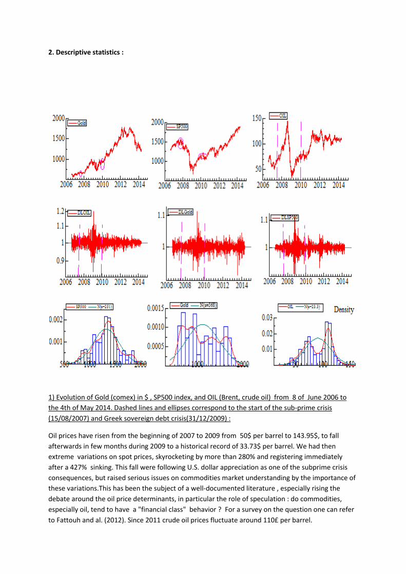
2. Descriptive statistics :

1) Evolution of Gold (comex) in $ , SP500 index, and OIL (Brent, crude oil) from 8 of June 2006 to

the 4th of May 2014. Dashed lines and ellipses correspond to the start of the sub-prime crisis

(15/08/2007) and Greek sovereign debt crisis(31/12/2009) :

Oil prices have risen from the beginning of 2007 to 2009 from 50$ per barrel to 143.95$, to fall

afterwards in few months during 2009 to a historical record of 33.73$ per barrel. We had then

extreme variations on spot prices, skyrocketing by more than 280% and registering immediately

after a 427% sinking. This fall were following U.S. dollar appreciation as one of the subprime crisis

consequences, but raised serious issues on commodities market understanding by the importance of

these variations.This has been the subject of a well-documented literature , especially rising the

debate around the oil price determinants, in particular the role of speculation : do commodities,

especially oil, tend to have a "financial class" behavior ? For a survey on the question one can refer

to Fattouh and al. (2012). Since 2011 crude oil prices fluctuate around 110£ per barrel.

The SP500 index is published by Standard and Poors (filial of Mc Graw Hill) since 1957, and is a

weighted average of the 500 most exchanged NYSE and NASDAQ stock market capitalizations. In

ellipse the SP500 index at the start of the subprime crisis (07/2007) and Greek Sovereign debt crisis

(31/12/2009). One can see the collapse of stock markets during the Great Depression and recovery

,reaching now the 2000 points (above the precedent record of 1500 points registered at the burst of

internet bubble in 2000.

Gold London closing fixing in $ (unit : troy oz) : We observe with clear evidence a sharp increase of

gold prices after the two crisis, used as a safe haven. Fixed-income investment, in particular U.S.

treasury bonds, followed by those of E.U. (cf. Greece, Spain, Portugal...) raised doubts on their

validity as being a safe diversification tool , which increased investment in commodities , as a LTDS.

We have reached a peak of 1795.1 $/Oz in February 2013, since then loosing 30% of its value. Is Gold

correlation with SP500 still the same? Or has the commodities investments being attractive pushed

Gold prices to behave differently?

2) Corresponding logreturns (DLOIL, DLGold and DLSP500) during the same period.

3) Density estimation with constant binwidth (=50), compared to a fitted normal.

One can see in (2) two periods of high volatility followed by period of low volatility in accordance

with stylized facts within financial time series. In (3) we will point out excess kurtosis and fat tails for

the SP500

Descriptive statistics on raw data :

Variable min mean max std.dev Normality Test : SP500 676.53 1325.1 1896.7 251.44 OIL 33.73 90.711 143.95 23.308 Gold 568.1 1118.1 1795.1 368.42 SP500 --------- Normality Test :

SP500 : Statistic t-Test P-Value Skewness 0.0043552 0.079931 0.93629 Excess Kurtosis -0.16733 1.5362 0.12448 Jarque-Bera 2.3606 0.30719 ARCH 1-2 test: F(2,2013) =3.0333e+005 [0.0000]** ARCH 1-5 test: F(5,2007) =1.2117e+005 [0.0000]** ARCH 1-10 test: F(10,1997)= 60523. [0.0000]**

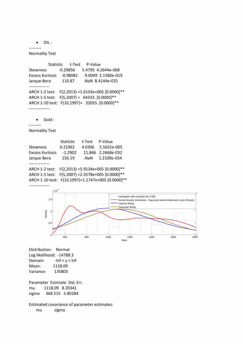
OIL : --------- Normality Test Statistic t-Test P-Value Skewness -0.29856 5.4795 4.2644e-008 Excess Kurtosis -0.98082 9.0049 2.1580e-019 Jarque-Bera 110.87 .NaN 8.4144e-025 --------------- ARCH 1-2 test: F(2,2013) =1.6103e+005 [0.0000]** ARCH 1-5 test: F(5,2007) = 64333. [0.0000]** ARCH 1-10 test: F(10,1997)= 32055. [0.0000]** ---------------

Gold : --------- Normality Test Statistic t-Test P-Value Skewness 0.21962 4.0306 5.5631e-005 Excess Kurtosis -1.2902 11.846 2.2668e-032 Jarque-Bera 156.19 .NaN 1.2100e-034 --------------- ARCH 1-2 test: F(2,2013) =5.9134e+005 [0.0000]** ARCH 1-5 test: F(5,2007) =2.3578e+005 [0.0000]** ARCH 1-10 test: F(10,1997)=1.1747e+005 [0.0000]** ---------------

Distribution: Normal Log likelihood: -14788.3 Domain: -Inf < y < Inf Mean: 1118.09 Variance: 135803 Parameter Estimate Std. Err. mu 1118.09 8.20341 sigma 368.515 5.80284 Estimated covariance of parameter estimates: mu sigma

600 800 1000 1200 1400 1600 18000

0.5

1

1.5

x 10-3

Data

Density

Histogram with constant bin (=50)

Kernel density estimation - Gaussian kernel-Silverman's rule of thumb

Gamma fitting

Gaussian fitting

mu 67.2959 -1.00042e-13 sigma -1.00042e-13 33.673 Distribution: Gamma Log likelihood: -14737.6 Domain: 0 < y < Inf Mean: 1118.09 Variance: 139343 Parameter Estimate Std. Err. a 8.97163 0.277347 b 124.625 3.96241 Estimated covariance of parameter estimates: a b a 0.0769213 -1.06852 b -1.06852 15.7007

Kernel: normal Bandwidth: 0.0998176 Domain: 0 < y < Inf

600 800 1000 1200 1400 1600 18000

0.1

0.2

0.3

0.4

0.5

0.6

0.7

0.8

0.9

1

Data

CDF fitting

Cum

ula

tive p

robabili

ty

Gold data

Kernel density estimation - Gaussian kernel-Silverman's rule of thumb

Gamma fitting

Gaussian fitting

-1,5

-1

-0,5

0

0,5

1

1,5 1

70

13

9

20

8

27

7

34

6

41

5

48

4

55

3

62

2

69

1

76

0

82

9

89

8

96

7

10

36

11

05

11

74

1

24

3

13

12

1

38

1

14

50

15

19

15

88

16

57

17

26

17

95

18

64

19

33

20

02

20

71

Cor(SP-OIL)

Cor(1-2)

-1

-0,5

0

0,5

1

1,5

1

79

15

7

23

5

31

3

39

1

46

9

54

7

62

5

70

3

78

1

85

9

93

7

10

15

10

93

11

71

12

49

13

27

14

05

14

83

15

61

16

39

17

17

17

95

18

73

19

51

20

29

COR(OIL-GOLD)

COR(2-3)

-2

-1

0

1

2

1

95

18

9

28

3

37

7

47

1

56

5

65

9

75

3

84

7

94

1

10

35

11

29

12

23

13

17

14

11

15

05

15

99

16

93

17

87

18

81

19

75

20

69

21

63

22

57

23

51

24

45

25

39

Cor(SP500-GOLD)

Cor(1-3)

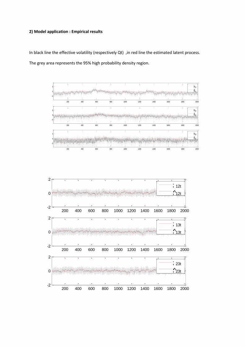
2) Model application : Empirical results

In black line the effective volatility (respectively Qt) ,in red line the estimated latent process.

The grey area represents the 95% high probability density region.

200 400 600 800 1000 1200 1400 1600 1800 2000

-5

0

5

h1t

h1t

200 400 600 800 1000 1200 1400 1600 1800 2000

-5

0

5

h2t

h2t

200 400 600 800 1000 1200 1400 1600 1800 2000

-5

0

5

h3t

h3t

200 400 600 800 1000 1200 1400 1600 1800 2000-2

0

2

; 12t

; 12t

200 400 600 800 1000 1200 1400 1600 1800 2000-2

0

2

; 13t

; 13t

200 400 600 800 1000 1200 1400 1600 1800 2000-2

0

2

; 23t

; 23t

We processed to only 500 iterations (hence with no burns) following the procedure in Casarin et al.

(2013).A good part of the starting iterations should have been eliminated and the number of

iterations increased (e.g. : 5000 iterations and 1000 burns) for more accurate results.

t

Samples from the posterior of s1t ; t = 1; : : : ; T

500 1000 1500 2000

100

200

300

400

500

1

1.2

1.4

1.6

0 500 1000 1500 2000 2500

0

1

2

3

Posterior mean of s1t ; t = 1; : : : ; T

t

Estimated

True

In red

the posterior mean, grey area the credibility interval. These outputs are useful to detect in our case

contagion effect, in the definition offered by Forbes and Rigobon(2009). One can see that we have

both increased volatility and high correlation during the beginning of the subprime crisis (last quarter

2007).

500 1000 1500 2000

-0.5

0

0.5

1

0

1

2

3

; 12t

st

500 1000 1500 2000

-0.5

0

0.5

1

0

1

2

3

; 13t

st

500 1000 1500 2000

-0.5

0

0.5

1

0

1

2

3

; 23t

st

500 1000 1500 2000-9

-4

0

4

0

1

h1t

s1;t

500 1000 1500 2000-9

-4

0

4

0

1

h2t

s1;t

500 1000 1500 2000-9

-4

0

4

0

1

h3t

s1;t

Computed posterior mean, regime switching, all along the studied period.

500 1000 1500 2000-0.5

0

0.5

1

Posterior mean of s1t; t = 1; : : : ; T

t

Conclusion :

Bibliography : R. Casarin, D. Tronzano, M. Sartore "A Bayesian Markov-switching correlation model for contagion analysis for contagion analysis on exchange rates markets (2013)". M.J. Lombardi ,F. Ravazzolo "Oil price density forecasts : exploring the linkages with stock markets (CAMP Working paper series,no3/2012)". Asai, McAleer " Bauwens L. , Laurent S.,Rombout J.V.K. (2006) " Multivariate GARCH models : asurvey",JoAE,21,79-109 Baillie R.T. Bollerslev T. (1989) "A multivariate generalized ARCH approach to modeling risk premia in forward exchange rate markets" +++ intro garch Baillie R.T.Bollerslev T. (1992) "Fractionally integrated generalized autoregressive conditionnal heteroskedasticity.++intro long-memory,figarch Engle (82) "Autoregressive conditional heteroskedasticity with estimates of the variance of united-Kingdom inflation",Econometrica,50,4,987-2007 Gourieroux Jasiak (2001) Financial econometrics, Princeton university Bolerslev (86) ,GARCH ,JOE. GARCH help offered in Oxmetrics, Mr. Laurent.

Internet sources :

http://commodityhq.com/2012/is-gold-still-a-safe-haven/