- C",,

/

/

!i

MARKOV REWARD PROCESSES: A FINAL REPORT

R. M. Smith

Department of Computer Science

Yale University

New Haven, CT. 01620

October 23, 1991

"--

5 3/ S -I

Abstract

Numerous applications in the area of computer system analysis can be effectively

studied with Markov reward models. These models describe the behavior of the system

with a continuous-time Markov chain, where a reward rate is associated with each state.

In a reliability/availability model, upstates may have reward rate 1 and down states

may have reward rate zero associated with them. In a queueing model, the number of

jobs of certain type in a given state may be the reward rate attached to that state. In

a combined model of performance and reliability, the reward rate of a state may be the

computational capacity, or a related performance measure. Expected steady-state rewardrate and expected instantaneous reward rate are clearly useful measures of the Markov

reward model. More generally, the distribution of accumulated reward or time-averaged

reward over a finite time interval may be determined from the solution of the Markov

reward model. This information is of great practical significance in situations where the

workload can be well characterized ( deterministically, or by continuous functions e.g.

distributions ).

The design process in the development of a computer system is an expensive andlong term endeavor. For aerospace applications the reliability of the computer system

is essential, as is the ability to complete critical workloads in a well defined real time

interval. Consequently, effective modeling of such systems must take into account both

performance and reliability. This fact motivates our use of Markov reward models to aidin the development and evaIuation of fault tolerant computer systems.

(NARA-CR-I_Q4_9) MARKOV REWARD PROCESSES

Final Report (Yale Univ.) 13 p CSCL 12A

G3/o5

NQ2-i374q

Unclas

0053185

*This work was supported by the NASA Langley Research Center under Grant NAG-I-_J

https://ntrs.nasa.gov/search.jsp?R=19920004526 2020-02-20T11:38:16+00:00Z

1 Introduction

In this annual report we summarize our research accomplishments under the auspices of the

NASA grant NAG-I-897 to develop tools and methods for the development of fast and reliable

computer/control systems.

The research effort has been focused in two directions, the development of mathematical

techniques and tools in order to enhance our understanding of relevant phenomena as well as

the use of these tools for the analysis of problems relevant to NASA's present or long termneeds.

2 Description of Markov Reward Models

Discrete-state continuous-time Markov chains are commonly used in the evaluation of

computer system performance as well as the reliability and availability of fault-tolerant sys-

tems. Such Markov models are often solved for either the steady-state or transient state

probabilities [26, 63]. Weighted sums of state probabilities are then used to obtain measures

of interest. In reliability/availability models the sum is taken over the set of operationalstates of the system. Since the operational states are a subset of all the possible states, the

weight attached to each state is either 0 or 1.

It is natural to extend the set of allowable weights to non-negative real numbers. For example,

when computing the average queue length in queueing models, the weight attached to a state

is a non-negative integer (the number of jobs in the queueing system). When we attach a

non-negative real number, called the reward rate, to each state of a Markov chain, we obtain

a Markov reward process. A second extension is to a class of interesting cumulative measures

that cannot be obtained as a weighted sum of state probabilities. In the reliability/availability

modeling of computer systems, these cumulative measures include the distribution of interval

availability (AI) and mean-time-to-failure (MTTF).

In many environments, computer systems are expected to provide service even though com-

ponent (or subsystem) failures may have occurred. In such fault-tolerant systems, the

performance, and the reliability are both important in determining the ability of a sys-

tem to deliver a specific amount of useful work in a finite time period. These considerations

are particularly relevant to switching systems, databases, and general purpose computer sys-

tems where graceful degradation and on-line repair of failed subsystems are common practice.

Thus, there are two aspects of the system to be dealt with, the state to state (configuration to

configuration) changes of the system over the interval (0, t) and the performance level (reward

rate) associated with each state of the system. The evolution of the system through different

configurations is characterized by a continuous-time Markov chain (CTMC) which will be

referred to as a structure-state process. Associated with each state of the CTMC of the

structure-state process is a reward rate to represent the performance level of the system in

that state (configuration). The set of reward rates associated with the states of a structure-

state process will be referred to as a reward structure. Thus each Markov reward model

(MKM) has a structure state process that characterizes the evolution of the system through a

set of states and a reward structure that characterizes the performance level associated with

eachstate.

Differentapplicationsgiveriseto differentinterpretationsof the underlyingCTMC and/or

different interpretations of the reward structure superimposed on the structure-state process.

If we interpret the reward rate to be the speed of service and the transition structure of the

CTMC to be failure and repair of components, the time needed to accumulate a fixed amount

of reward will be the time to complete a task with a fixed work requirement in a failure-prone

environment. From the distribution of the task-completion-time, we can derive quantities

such as the probability of ever completing the task or the probability of completing the task

before a given deadline. If we interpret the structure of the CTMC as modeling the arrival

and departure of tasks in a queueing system, and interpret the reward rate as the number of

jobs in the queue, we can obtain the time-averaged queue length distribution. By interpreting

the structure-state process as task arrival/departure and interpreting the reward rate as the

portion of the server capacity allocated to a 'tagged' job, the completion-time distribution will

yield the response time distribution in the queueing system. The general utility of Markov

reward modeling thus stems from the ability to assign and interpret both the structure-state

process and the reward structure appropriately for a wide range of situations.

Even after interpretations of the CTMC and reward structure have been made, a wide va-

riety of measures may be obtained from the MRM. Choosing an appropriate measure for

an application is important. Since the computational cost of obtaining the measures varies,

generally the easiest to compute appropriate measure is best. Measures can characterize

system behavior in a cumulative way (total work done in a given utilization period) or at

an instant of time. For some applications, long range equilibrium behavior is more relevant,

while for others transient conditions in the time interval shortly after system start up are

more important. Finally, an expected value may be acceptable to answer some questions,

while for other questions more detailed distributional information may be required. Before

we more fulIy discuss various models and measures we introduce some standard notation for

the structure state process CTMC, define some useful cumulative and instantaneous random

variables, and present a small expository example in the next subsection.

2.1 Notation

The evolution of the system in time is represented by a finite-state stochastic process {Z(t), t _>

0}. Titus Z(t) is the structure-state of the system at time t and Z(t) E S = {1,2,...,n}.

The holding times in the structure-states are exponentially distributed and hence Z(t) is a

homogeneous CTMC. Even in situations where the holding times are generally distributed,

they may often be acceptably approximated using a finite number of exponential phases

[15, 29]. We let q{j, 1 <_ i,j <_ n, be the infinitesimal transition rate from state i to state j

and Q = [qij] is the n by n generator matrix where

I%

qii = -- _ qij.j=l,j_i

For the sake of clarity we also define ql = -qii. A fixed reward rate ri is associated with each

structure-state i, and the vector _.rdefines the reward structure. To represent the reward rate

of the system at time t, we let X(t) = rz(t). Finally, we let pi(t) denote P[ Z(t) = i ], the

probability that the system is in state i at time t. The state probability vector p_p_(t)may be

computed by solving a matrix differentia] equation [26],

dd-7 p_(t) = p_(t) 0,.

3

Methodsfor computing_(t) arecomparedin [48].

A fundamentalquestionabout any system is simply, "What is the probability of completing a

given amount of useful work within a specified time interval?" We let Y(t) be the accumulated

reward until time t, that is, the area under the X(t) curve,

_0 _Y(t) = X(v)dr.

The value of Y(t) is the amount of reward accumulated by a system during the interval (0, t).

Consequently, by interpreting rewards as performance levels, we see that the distribution of

accumulated reward is at the heart of characterizing systems that evolve through states with

different reward rates (e.g., performance levels). In Figure 1 we depict a Markov reward

model with a 3-state CTMC for the structure-state process and a simple reward structure,

the transition rate matrix of the CTMC, as well as sample paths for the stochastic processes

Z(t), X(t) and Y(t). Note that a given sample path of Z(t) determines unique sample paths

for X(t) and Y(t).

We denote the distribution of accumulated reward at time t evaluated at z as:

y(z,t)- P[ Y(t) < z 1.

When the CTMC Z(t) has one or more absorbing states with a zero reward rate, we may

also wish to compute the distribution of accumulated reward until absorption,

_--P[r(o ) <_• 1.

The time average of Y(t) and the distribution of the time-averaged accumulated reward aredenoted as:

1/o'w(t) = 7 and w(., t) - P[ w(t) <_• ].

The distribution of time-averaged accumulated reward is particularly useful for comparing

the behavior of a system over time intervals of different length. To complete our notation, we

note that we have assumed a distinguished initial state. To explicitly indicate this dependence

on the initial state we will use a subscript on cumulative and time-averaged random variables

and their distributions. For example, Yi(t) denotes the accumulated reward for the interval

(0, t) given that the initial state is i, (i.e., Z(O) = i).

In the special case when we assign a reward rate 1 to operational states and zero to non-

operational states, the expected reward rate at time t, E[X(t)], is known as the instantaneous

or point availability A(t), the expected reward rate in the steady-state, E[X(oo)], is called

the steady-state availability A((x_) and W(t) is called the interval availability Al(t).

For a more complete description of the historical development, notation, measures and models

see [60].

Markov models have been used for the reJJability and availability analysis of computer�communication

systems [52, 55, 63]. More recently, Markov reward models have been used for the combined

evaluation of performance and reliability [3, 6, 11, 29, 39, 58]. Our exposition of Markov

reward models used them not only in the combined evaluation of performance and reliability

but in many other problems of computer/communications systems analysis. Until recently

distributions of cumulative measures and their time-averages were only obtainable for small

or special Markovian systems. The use of Markov reward models extends our ability to model

4

z(t)

3

] I I I •

tZ(t) Path

rl ---- 2.0 r2 = 1.0 r3 = 0.02A A

Markov Reward Model

Q

-2X 2X 0

_2 -(_2+A) A

0 #3 --_3

x(t)

3

Y(t)

4

3

I p

tX(t) Path

I [

/

Y(t) Path

I ] "t

Figure 1: 3-State Markov Reward Model with Sample Paths of Z(t), X(t) and Y(t) Processes.

suchsystemsand with the algorithmsin [58,50]wehaveobtainednewanduseful results.

We have illustrated the wide applicability of Markov reward models and the effectiveness

of our algorithm with a variety of examples in the area of computer systems analysis. By

interpreting the structure-state process as the failure and repair behavior of components and

the reward structure as the ability of the system to render useful service, we obtain per-

formability measures of practical interest such as the distribution of accumulated reward or

the completion time distribution depending on whether the time or reward requirement is

fixed. If we interpret the structure-state process as characterizing the arrival and departure

behavior of tasks in a queueing system, interpret the reward structure as the number of jobs

in the queue and fix the time interval considered then we obtain the time-averaged queue

length distribution. If we interpret the structure-state process as delineating the arrival and

departure behavior of tasks in a queueing system, interpret the reward structure as the por-

tion of service rendered to a 'tagged' job, and fix the reward requirement then we obtain the

response time distribution of an M/M/1/k/PS queueing system.

As the examples in papers [58, 60] show, the results can be used to make quantitative state-

ments about the ability of computer systems to complete fixed amounts of work in a given

time interval The next few sections introduce the notion of a critical workload, and use a

well characterized Workload disatribution distribution to obtain critical workload completion

probabilities.

3 Modeling and Critical Workloads

The design process in the development of a computer system is an expensive and long

term endeavor. For aerospace applications the reliability of the computer system is essential,

as is the ability to complete critical workloads in a well defined real time interval. Conse-

quently, effective modeling of such systems must take into account both performance and

reliability. The early use of models in the design of such complex computer systems can

substantially improve the quality of the final result, as well as decrease costs. Whether a

model is analytic, a simulation, or a prototype a well constructed model will yield insight

into the functional capabilities of the components and their effect on the system as a whole.

Often models can be used to find weaknesses and errors early in the design process, where

they can be most easily and inexpensively rectified.

We view a computer system as having three levels

• hardware resources

• an operating system to correctly and efficiently manage the hardware resources

• applications that request resources in order to compute "responses".

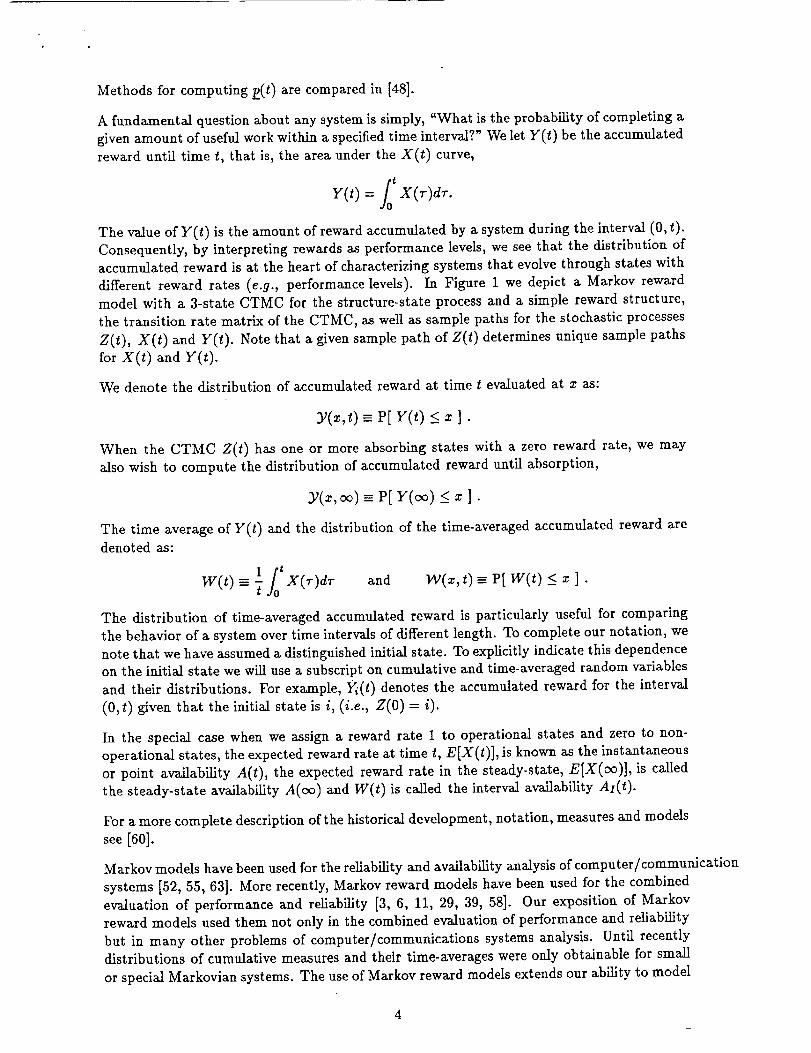
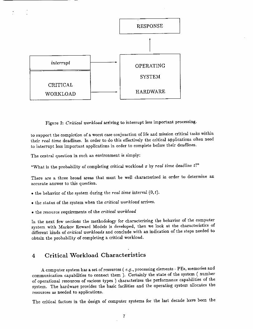
The conceptual environment of the critical workloads ( applications whose timely completion

is essential to continued safe operation ) is shown in Figure 2.

The completion time of an application depends on the ability of the hardware and operating

system to meet the resource requirements of the application in a timely fashion. Often, the

performance bottleneck (/.e. limiting ) requirements are memory access speeds and floating

point computation speeds. On a loosely coupled or distributed system where the workload is

composed of life critical, mission critical and non-critical applications there must be resources

6

RESPONSE

interrupt

CRITICAL

WORKLOAD

OPERATING

SYSTEM

HARDWARE

Figure 2: Critical workload arriving to interrupt less important processing.

to support the completion of a worst case conjunction of life and mission critical tasks within

their real time deadlines. In order to do this effectively the critical applications often need

to interrupt less important applications in order to complete before their deadlines.

The central question in such an environment is simply:

"What is the probability of completing critical workload z by real time deadline t?"

There are a three broad areas that must be well characterized in order to determine an

accurate answer to this question.

• the behavior of the system during the real time interval (0, t).

• the status of the system when the critical workload arrives.

• the resource requirements of the critical workload

In the next few sections the methodology for characterizing the behavior of the computer

system with Markov Reward Models is developed, then we look at the characteristics ofdifferent kinds of critical workloads and conclude with an indication of the steps needed to

obtain the probability of completing a critical workload.

4 Critical Workload Characteristics

A computer system has a set of resources ( e.g., processing elements - PEs, memories and

communication capabilities to connect them ). Certainly the state of the system ( number

of operational resources of various types ) characterizes the performance capabilities of the

system. The hardware provides the basic facilities and the operating system allocates the

resources as needed to applications.

The critical factors in the design of computer systems for the last decade have been the

7

ability to access and process data. In many ways, the evolution of computer architectures

has been an account of new ways to remove limitations on both these capabilities. Most

computer applications are one of 2 classes of computation.

Computational programs ( e.g., scientific, engineering control ) that take parameters and

perform arithmetic/logical operations with them to produce a result that is expressed in afew numbers.

Data-based programs on the other hand, access large data-sets to gain limited information

which is then read/modified. Examples would be updating the coverage of an insurance policy

in a large data base or updating a few elements of a large array.

Most programs tend to be either in one class or the other. Real time control programs

tend to generate computational workloads, which suggests CPU rate ( mips or flops ) as

an appropriate performance measure. Large-scale scientific computations in areas such as

high speed vehicle design and structural/electronic/optical design or testing tend to involve

large arrays and as such take on some of the characteristics of data-based programs, making

memory bandwidth an important consideration as well. In cases where the performance

bottleneck is not clear, a more detailed examination of the performance characteristics of the

system under the types of workload in question can be used to determine performance levels.

Interrupts insure that critical workloads will receive immediate attention, thereby making

the delay until a critical workload is serviced very small. The small delay can be taken into

account by lowering the deadline time t. In such a situation, the performance bottleneck ofa critical real time control workload will be CPU rate.

Clearly the computational requirements of a critical workload will strongly effect the prob-

ability of completing it be a real time deadline t. To some extent the size of the critical

workload will depend on the input that generated it. A conservative assumption would be

that the critical workload resulted from a worst case set of inputs. If more information on the

critical workload distribution is available, a more accurate determination of the probability

of completing it by a real time deadline would be possible.

Therefore let us define the critical workload size distribution through its density function:

B(x) = P[ critical workload size = x ] .

The conservative worst case approach for a maximum workload, 0, can be represented as

B(x) = _f(x-O), setting the probability that x is 0 to 1. Other critical workload models might

include normally distributed, since in the absence of hard data the central limit theorem gives

some justification for this model. Of course empirical distributions obtained from running

the critical workload on representative portions of the input space could be used as well.

If we regard the critical workload as the sum of the instructions executed for a given set of

input data then we would expect the size of the critical workload, x to be appro_mately

normally distributed because of the central limit theorem. Even though the central limit

theorem assumes the independence of the random variables ( instruction workloads ) to show

the asymptotically normal behavior of the sum, x. However, for many applications there

is a control portion of the code that takes as input the data and chooses the appropriate

execution path given the data. Often this is done with an eye to using very efficient methods

where possible. A consequence of the presence of this upper level control structure is that

the workload distribution will be multi-modal. A reasonable quantitative characterization of

the improvement of the completion time distribution resulting from implementation of highly

efficient solution methods for a subset of the possible inputs is valuable contribution.

8

5 Critical Workload Completion Probabilities

In section 2 we introduced Markov reward models and the complementary distribution

of accumulated reward Yc(z,t), and a method to obtain 7-(0), the initial state probabilityvector of the Markov reward model. In section 3 we discussed several simple densities of

critical workload size, B(x). To obtain the unconditional probability of completing a critical

workload (CW)with density B(z), we need only uncondition over z, thus:

P[ CW completes by t ] = ye(z, t)B(z)dx. (1)

For a conservative estimate of the workload completion probability, B(x) = _(x - 0) and

7_(0) is such that P[ min configuration ] = 1. This reduces equation (4) to Yc(0, t) with 7_(0)such that the configuration when the job arrives is the minimal operational configuration. A

refined estimate is possible by more realistically characterizing the workload density, B(z)

and more accurate determination of 7(0) at the time the critical workload arrives.

Where the consequences of failure to complete critical workloads by a real time deadline are

grave and the cost Of insuring timely completion are high, it is essential that effective tools

to analyze the situation are developed to make the most of available hardware and human

resources in the development and production of high performance fault tolerant systems. For

results using this methodological approach and several interesting examples see [59]

6 Conclusion

Four interesting models are developedfrom which we obtain the following distributions, multi-

processor performability, task completion time in a failure prone environment ( a semi-Markov

model ), the response time in a processor sharing disciplined queueing system, and the time

averaged queue length for a M/M/1/k queue. The final model is also used as an example to

indicate hereto unknown dynamic behavior of the M/M/1/k queue ( Sect. 5.1 in [60]).

Workload characterization, and the completion time distribution of workloads in various

environments is then examined in [59].-

Further details on the computational aspects of Markov reward models are available in [48,

49, 50, 57, 58]. My current interests also include using approximation techniques, such as

those indicated in [1] to improve the computational efficiency and accuracy of the hyperbolic

PDE performability equation. Computation of the distribution of task completion time with

a possible loss of work upon failure is treated in [8, 10, 36, 37, 42]. The question of the

generation of the Markov models for large systems is addressed in [2, 11, 20, 22, 51].

References

[1] D. Aldous. Probability Approzimation Via the Poisson Clumping Heuristic. Springer-

Verlag, New York, NY, 1989.

[2] S. J. Bavuso, J. B. Dugan, K. S. Trivedi, E. M. Rothmann, and W. E. Smith. Analysis

of Typical Fault-Tolerant Architectures Using HARP. IEEE Transactions on Reliability,

R-36(2):176-185, June 1987.

9

[3] M. D. Beaudry. Performance Related Reliability for Computer Systems. IEEE Trans-

actions on Computers, C-27(6):540-547, June 1978.

[4] D. P. Bhandarkar. Analysis of Memory Interference in Multiprocessors. IEEE Transac-

tions on Computers, C-24(11):897-908, November 1975.

[5] U. N. Bhat. A Study of Queueing Systems M/G/1 and GI/M/1. Lecture Notes in

Operation Research and Mathematical Economics, Volume 2, Springer-Verlag, Berlin,1968.

[6] J. Blake, A. Reibman and K. Trivedi. Sensitivity Analysis of Reliability and Perfroam-

nee Measures for Multiprocessor Systems. 1988 ACM SIGMETRICS Conference on

Measurement and Modeling of Computer Systems, Santa Fe, NM, May 1988.

[7] J. P. C. Blanc and E. A. Van Doom. Relazation Times for Queueing Systems. Technical

Report OS-R8407, Centre for Mathematics and Computer Science, 1987.

[8] A. Bobbio and K. Trivedi. Computation of the Distribution of the Completion Time

when the Work Requirement is a PH Random Variable. Stochastic Models, to appear.

[9] W.G. Bouricius, W.C. Carter and P.R. Schneider. Reliability Modeling Techniques for

Self-Repairing Computer Systems. Proceedings of the $_th National Conference of the

ACM, pp. 295-309, 1969.

[10] P. F. Chlmento. System Performance in a Failure Prone Environment. PhD thesis,

Department of Computer Science, Duke University, Durham, NC, November 1988.

[11] G. Ciardo, J. Muppala and K.S. Trivedi. SPNP: Stochastic Petri Net Package. Third

International Workshop on Petri Nets and Performance Models, Kyoto, 1989.

[12] G. Ciardo, R. Marie, B. Sericola, and K.S. Trivedi. Performability Analysis Using Semi-

Markov Reward Processes. IEEE Transactions on Computers, to appear.

[13] E. G. Coffman, R. R. Muntz and H. Trotter. Waiting Time Distributions for Processor

Sharing Systems. Journal for the Association of Computing Machinery, 17(1):123-130,January 1970.

[14] J. W. Cohen. The Single Server Queue. North-tIolland, New York, NY, 1982.

[15] D. R. Cox. A Use of Complex Probabilities in the Theory of Stochastic Processes. Proc.

Cambridge Phil. Soc., 51:313-319, 1955.

[16] E. de Souza e Silva and R. Gaff. Calculating Cumulative Operational Time Distributions

of Repairable Computer Systems. IEEE Transactions on Computers, C-35(4):322-332,

April 1986.

[17] E. de Souza e Silva and It. R. GaJl, "Calculating Availability and Performance Measures

of Repairable Computer Systems Using Randomization," Journal for the Association of

Computing Machinery, 36(1):171-193, January 1989.

[18] L. DonatieUo and B. R. Iyer. Analysis of a Composite Performance l_eliability Mea-

sure for Fault-Tolerant Systems. Journal for the Association of Computing Machinery,

34(1):179-199, January 1987.

[19] D. G. Furchtgott and J. F. Meyer. A Performability Solution Method for Degradable

Nonrepairable Systems. IEEE Transactions on Computers, C-33(6):550-554, June 1984.

10

[20] It. Geist and K. S.Trivedi. Ultra-High Reliability Predictionfor Fault-TolerantCom-puter Systems.IEEE Transactions on Computers, C-32(12):1118-1127, December 1983.

[21] A. Goyal and A. N. Tantawi. Evaluation of Perfomability in Acyclic Markov Chains.

IEEE Transactions on Computers, C-36(6):738-744, June 1987.

[22] A. Goyal, W. C. Carter, E. de Souza e Silva, S. S. Lavenberg, and K. S. Trivedi. The

System Availability Estimator. In Proceedings of the Sixteenth International Symposium

on Fault-Tolerant Computing, pp. 84-89, July 1986.

[23] A. Goyal, A. Tantawi, and K. Trivedi. A Measure of Guaranteed Availability. IBM

Itesearch Iteport ItC 11341, IBM T. J. Watson Itesearch Center, 1985.

[24] W. Grassmann. Transient Solution in Markovian Queueing Systems. Computers and

Operation Research, 4:47-56, 1977.

[25] W. K. Grassmann. Means and Variances of Time Averages in Markovian Environments.

European J. of Operations Research, 31(1):132-139, 1987.

[26] D. Gross and C. M. Harris, Fundamentals of Queueing Theory, John Wiley and Sons,

New York, 1985.

[27] A. Hordijk, D. L. Iglehart, and It. Schassberger. Discrete Time Methods for Simulat-

ing Continuous Time Markov Chains. Advances in Applied Probability, 8(4):772-788,December 1976.

[28] P_. A. Howard. Dynamic Probabilistic Systems, Volume II: Semi-Markov and Decision

Processes. John Wiley and Sons, New York, 1971.

[29] M. C. Hsueh, It. K. Iyer, and K. S. Trivedi. Performability Modeling Based on Real

Data: a Case Study. IEEE Transactions on Computers, C-37(4), April 1988.

[30] It. Huslende. A Combined Evaluation of Performance and Reliability for Degradeable

Systems. In ACM/SIGMETRICS Conf. on Measurement and Modeling of Computer

Systems, pp. 157-164, ACM, 1981.

[311 B. It. Iyer, L. Donatiello and P. Heidelberger. Analysis of Performability for Stochastic

Models of Fault-Tolerant Systems.IEEE Transactions on Computers, C-35(10):902-907,October 1986.

[32] S. Karlin and J. L. MacGregor. Ehrenfest Urn Models. Journal of Applied Probability,

2(2):352-376, 1965.

[33] C. M. Krishna and K. G. Shin. Performance Measures for Multiprocessor Controllers.

Performance'83, Agrawaia and Tripathi (eds.), North-Holland, 1983, pp. 229-246.

[34] V. G. Kulkarrd, V. F. Nicola, and K. S. Trivedi. On Modeling the Performance and

Reliability of Multi-Mode Computer Systems. The Journal of Systems and Software,

6(1 & 2):175-183, May 1986.

[35] V. G. Kulkarni, V. F. Nicola, It. M. Smith and K. S. Trivedi. Numerical Evaluation of

Performability and Job Completion Time in Repairable Fault-Tolerant Systems. FTCS

Proceedings, Vol.16, 1986, pp. 252-257.

[36] V. G. Kulkarni, V. F. Nicola, and K. S. Trivedi. The completion time of a job on multi-

mode systems. Advances in Applied Probability, 19:932-954, December 1987.

11

[37]

[38]

[39]

[4o]

V. G. Kulkarni, V. F. Nicola, and K. S. Trivedi. Effects of Checkpointing and Queueing

on Program Performance. Stochastic Models, to appear.

J. F. Meyer. On Evaluating the Performability of Degradable Computer Systems. IEEE

Transactions on Computers, C-29(8):720-731, August 1980.

J. F. Meyer. Closed-form Solutions of Performability. IEEE Transactions on Computers,

C-31(7):648-657, July 1982.

J. F. Meyer. Performability Modeling of Distributed Real Time Systems. Mathematical

Computer Performance and Reliability, G. Iazeolia, P.J. Courtois and A. Hordljk (eds.),

Elsevier Science Publishers (North Holland), 1984, pp. 361-372.

[41] P. M. Morse. Stochastic Properties of Waiting Lines. Operations Research, 2(3):255-261,1955.

[42]

[43]

[44]

[45]

[46]

[47]

[48]

[49]

[50]

[5i]

[52]

[53]

V. F. Nicola, V. G. Kulkarni, and K. S. Trivedi. Queueing Analysis of Fault-Tolerant

Computer Systems. IEEE Transactions on Software Engineering, SE-13(3):363-375,March 1987.

A. 1t. Odoni and E. Roth. An Empirical Investigation of the Tansient Behavior of

Statioary Queueing Systems. Operations Research, 31:432-455, May-June 1983.

E. Parzen. Stochastic Processes. Holden-Day, San Francisco, CA, 1962.

K. Pattipati and S. Shah. On the Computational Aspects of Performability Models of

Fault-Tolerant Computer Systems. IEEE Transactions on Computers, to appear.

K. Pattipati, Y. Li and g. Blom. On the Reliability and Performability of Fault-Tolerant

Computer Systems. Technical Report, Dept. of Elect. and Systems Engg., Univ. of Con-

necticut, 1989.

P. S. Purl. A Method for Studying the Integral Functionals of Stochastic Processes with

Applications: I. The Markov Chain Case. Journal of Applied Probability, 8(2):331-343,June 1971.

A. Keibman and K. S. Trivedi. Numerical transient analysis of Markov models. Comput-

ers and Operations Research, 15(1):19-36, 1988.

A.L. Reibman and K.S. Trivedi. Transient Analysis of Cumulative Measures of Markov

Model Behavior. Stochastic Models, 5(4), 1989.

A. Reibman, R. Smith and K. Trivedi. Markov and Maxkov Reward Models: A Survey

of Numerical Approaches. European Journal of Operations Research,40:257-267, 1989.

R.Sahner and K. S. Trivedi. Reliability Modeling Using SttARPE. IEEE Transactions

on Reliability, R-36(2):186-193, June 1987.

M. L. Shooman. Probabilistic Reliability: An Engineering Approach. McGraw-Hill, New

York, 1968.

D. Siewiorek. Multiprocessors: Reliability Modelling and Graceful Degradation. In

Infotech State of the Art Conference on System Reliability, pp. 48-73, Infotech Interna-

tional, Ltd., Infotech International, London, 1978.

12

[54]

[55]

[56]

[57]

[58]

f59j

[6o]

[61]

[62]

[63]

[64]

[65]

[66]

[67]

D. P. Siewiorek, V. Kini, R. Joobbani, and H. Bellis. A Case Study of C.mmp, Cm*,

and C.vmp: Part II -- Predicting and Calibrating Reliability of Multiprocessor Systems.

Proceedings of the IEEE, 66(10):1200-1220, October 1978.

D. P. Siewiorek and R. S. Swarz. The Theory and Practice of Reliable System Design.

Digital Press, Bedford, MA, 1982.

R. M. Smith and K. S. Trivedi. A Performability Analysis of Two Multiprocessor Sys-

tems. In Proceedings of the Seventeenth International Symposium on Fault-Tolerant

Computing, pp. 224-229, July 1987.

R. M. Smith. Markov Reward Models: Application Domains and Solution Methods. PhD

thesis, Department of Computer Science, Duke University, Durham, NC, September1987.

R. M. Smith, K. S. Trivedi, and A. V. Ramesh. Performability Analysis: Measures, an

Algorithm and a Case Study. IEEE Transactions on Computers, C-37(4):406-417, April1988.

R. M. Smith and J. A. Sjogren Three ReM-Time Architectures: A Study Using Reward

Models. ICAS-90-2.4._ Proceedings, Stockholm, Sweden, Vol. 17, Sept 1990.

R. M. Smith and K. S. Trivedi. The Analysis of Computer Systems Using Markov Reward

Models Stochastic Analysis of Computer and Communications Systems , ed.

by Hideaki Takagi, pp. 589-629, Elsevier Science Publishing, 1990.

T. E. Stern. Approximations of Queue Dynamics and Their Application to Adaptive

Routing in Computer Communication Networks. IEEE Transactions on Communica-

tions, COM-27(9):1331-1335, September 1979.

U. Sumita, J. G. Shanthikumar, and Y. Masuda. Analysis of Fault Tolerant Computer

Systems. Microelectronics and Reliability, 27:65-78, 1987.

K. S. Trivedi. Probability and Statistics with Reliability, Queuing, and Computer Science

Applications. Prentice-Hall, Englewood Cliffs, NJ, 1982.

W. Whitt. Untold Horrors of the Waiting Room: What the Equilibrium Distribution

Will Never Tell About the Queue Length Process. Management Science, 29(4):395-408,

April 1983.

R. W. Wolff. Poisson Arrivals See Time Averages. Operations Research, 30(2):223-231,

March-April 1982.

C-L. Wu. Operational Modes for the Evaluation of Degradeable Computing Systems.

A CM SIGMETRICS Conference on Measurement and Modeling of Computer Systems,

pp. 179-185, August-September 1982.

M. Veeraxaghavan and K. Trivedi. Hieraxchical Modeling for Reliability and Perfor-

mance Measures. Concurrent Computations: Algorithms, Architectures and Technology.

S. Tewksbury, B. Dickson and S. Schwartz (eds.), Plenum Press, NY, pp. 449-474, 1987.

13