Markov Networks - GitHub Pages
15
Transcript of Markov Networks - GitHub Pages

CMPUT 651 (Fall 2019)
Pros & Cons of HMMPros
• Model the relationship among different time steps
• Implicit clustering
- Not based on the similarity of observations themselves (cf. GMM)
- But based on similarity of observations in state transition
• Support unsupervised training. E.g.,
- States={rainy, snowy, sunny}
- Observations={wet, icy, dry}
S1 S2
x1 x2
S3
x3

CMPUT 651 (Fall 2019)
Pros & Cons of HMMCons
• The discriminative classification is over-simplified (can be addressed by reverse to and incorporate more features)
• Label bias problem
s → xx → s
S1 S2
x1 x2
S3
x3
Source: http://www.cs.cmu.edu/~epxing/Class/10708/lectures/lecture12-CRF.pdf

CMPUT 651 (Fall 2019)
Undirected Graph• Idea: Each local factor yields a scoring
function, instead of a probability
• Normalizing the probability afterwards
S1 S2
x1 x2
S3
x3
Source: http://www.cs.cmu.edu/~epxing/Class/10708/lectures/lecture12-CRF.pdf

CMPUT 651 (Fall 2019)
Markov Random Field• Let be the nodes
• The scope of a factor is a subset of :
, where
• A factor maps the values of a scope to a non-negative/positive number
V = {X1, X2, ⋯, XN}
ϕi V
{Xi,1, ⋯, Xi,ni} Xi,j ∈ V
ϕi : Xi,1, Xi,2, ⋯, Xi,ni→ ℝ+
Suppose we have factors in total
Def (unnormalized measure):
Def (partition function):
Def (Probability):
K
p̃(x1, ⋯, xn) =K
∏k=1
ϕk(xk,1, ⋯, xk,nk)
Z = ∑x1,⋯,xn
p(x1, ⋯, xn)
p(x1, ⋯, xn) =1Z
p̃(x1, ⋯, xn)
(Also model parameters)

CMPUT 651 (Fall 2019)
Markov Network• Let be the nodes
• The scope of a factor is a subset of :
, where
• A factor maps the values of a scope to a non-negative/positive number
• A Markov network (induced by the MRF) is an undirected graph , where
V = {X1, X2, ⋯, XN}
ϕi V
{Xi,1, ⋯, Xi,ni} Xi,j ∈ V
ϕi : Xi,1, Xi,2, ⋯, Xi,ni→ ℝ+
G = ⟨V, E⟩
E = {(i, j) : ∃k, {xi, xj} ⊆ scope(ϕk)

CMPUT 651 (Fall 2019)
Markov Random FieldInterpretation of the factors
• Local happiness for a certain assignment
• Not probability:
• Not marginal probability:
• Posterior is local [HW1]
Hint: , where is a multiplication of many factors,
which in turn can be grouped into two categories: those including and those not including . The latter is canceled out in both the numerator and the denominator.
p(x1, x2) ≠ϕ(x1, x2)
∑x1,x2ϕ(x1, x2)
p(x1, x2) ∝/∑x2
ϕ(x1, x2)
p(xi |x−i) ∝ ∏k:xi∈scope(ϕk)
ϕk
p(xi |x−i) =p(xi, x−i)
∑x′�ip(x′�i, x−i)
p( ⋅ )
XiXi

CMPUT 651 (Fall 2019)
Application of MRF• No explicit “cause and effect”
- Entangled photons
- Image pixels
- Even in a sentence, a preceding word may not be a cause
- Social network: everyone is influencing everyone else simultaneously
- HW2: Give your own example. What else is more suitable to be modeled as an MRF than a BN? And why?

CMPUT 651 (Fall 2019)
Log-Linear Model• Another parametrization of the MRF
p(x1, ⋯, xn) ∝n
∏i=1
ϕ(xi,1, ⋯, xi,ni)
= exp{n
∑i=1
log ϕi(xi,1, ⋯, xi,ni)}
= exp{n
∑i=1
∑x′ �i,1,⋯,x′�i,ni
log ϕi(x′�i,1, ⋯, x′�i,ni)𝕀{xni
, ⋯xni= x′�ni
, ⋯, x′�ni})}
θ fParameters Features
p(x1, ⋯, xn) =1Z
exp{∑i
θi fi(x)}
The same as MN (suppose potentials >0)

CMPUT 651 (Fall 2019)
Learning• Unlike BN, MRF’s weights can never be manually assigned
- Humans are especially bad at expressing our vague intuition
• MRF’s weights have to be learned in some principled way
Maximum likelihood estimation (MLE): 1N ∑
j
log p(x( j)) =1N ∑
j
log1Z
exp{∑i
θi fi(x( j))}∂
∂θi
1N ∑
j
log1Z
exp{∑i
θi fi(x( j))}
=∂
∂θi
1N ∑
j
log exp{∑i′�
θi′ � fi(x( j))} −∂
∂θi
1N ∑
j
log∑x′ �
exp{∑i′�
θi′ � fi′�(x′�)}
=1N ∑
j
fi −1
∑x′ �′ �exp{∑i θi fi(x′�′�)} ∑x′�
exp{∑iθi fi(x′ �)}fi(x′ �)
=1N ∑
j
fi − ∑x′�
exp{∑i θi fi(x′�)}∑x′ �′ �exp{∑i θi fi(x′�′�)}
fi(x′�)
= 𝔼x∼𝒟[ fi] − 𝔼x∼pθ(x)[ fi(x)]Expectation in data — Expectation in model
CMPUT 651 (Fall 2019)
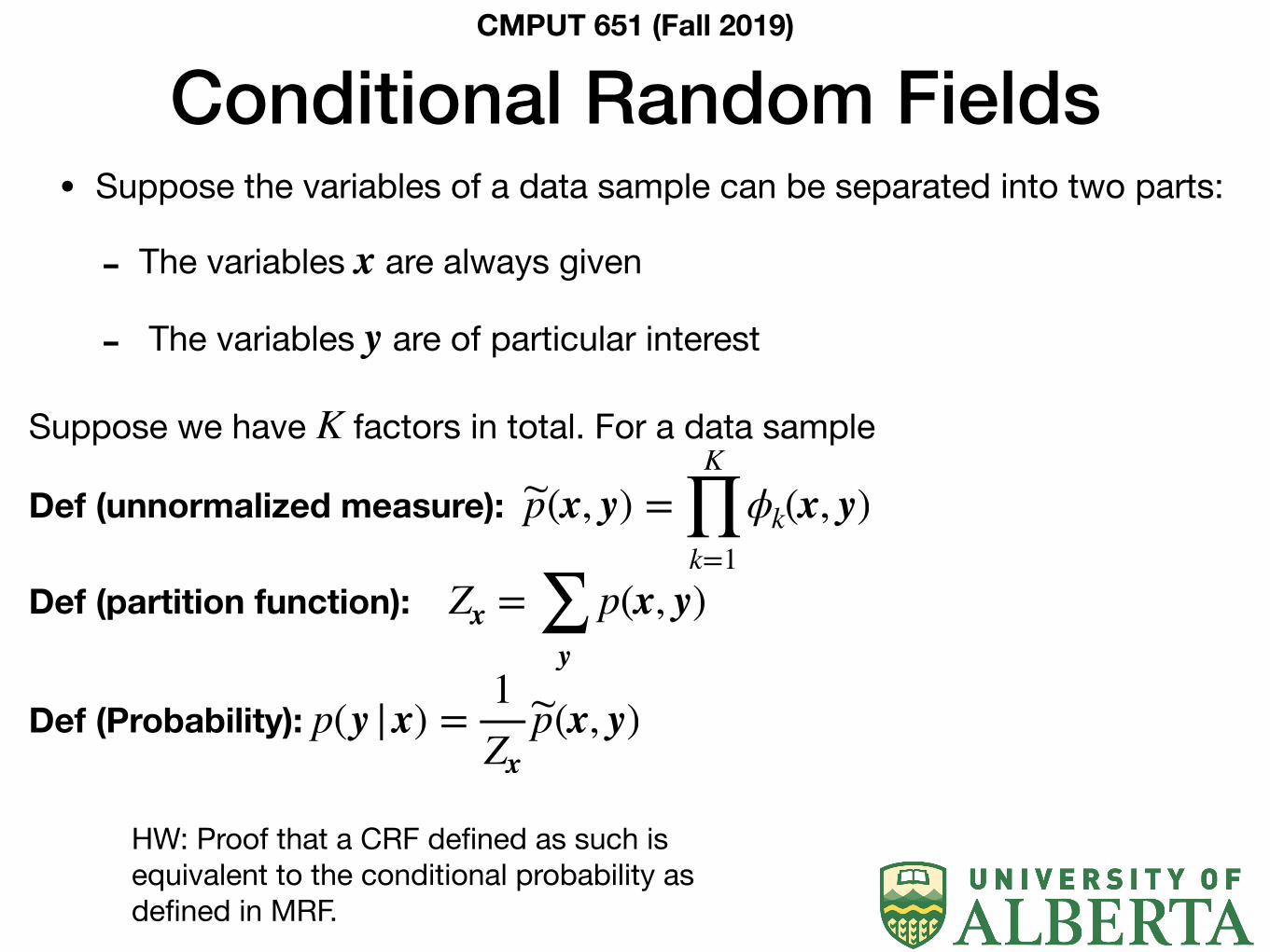
Conditional Random Fields• Suppose the variables of a data sample can be separated into two parts:
- The variables are always given
- The variables are of particular interest
x
y
Suppose we have factors in total. For a data sample
Def (unnormalized measure):
Def (partition function):
Def (Probability):
K
p̃(x, y) =K
∏k=1
ϕk(x, y)
Zx = ∑y
p(x, y)
p(y |x) =1Zx
p̃(x, y)
HW: Proof that a CRF defined as such is equivalent to the conditional probability as defined in MRF.

CMPUT 651 (Fall 2019)
Conditional Random Fields• Suppose the variables of a data sample can be separated into two parts:
- The variables are always given
- The variables are of particular interest
- MLE: maximizing
x
y
p(y |x)
∂∂θi
log p(x(i))
= 𝔼x∼𝒟[ fi] − 𝔼x∼pθ(x)[ fi(x)]
Expectation in data — Expectation in model (in CRF, given evidence of a particular data point)
MRF: CRF:
∂∂θi
log p(x(i))
= 𝔼x∼𝒟[ fi] − 𝔼x∼pθ(x)[ fi(x)]y(i) y y y
x(i)Given each data sample
y
y ∼ pθ(y |x)This sample

CMPUT 651 (Fall 2019)
Inference• In general: Hard
• Chain MRF/CRF: DP as for HMM

• PGM course
https://www.youtube.com/watch?v=q8vNcVmarcI&feature=youtu.be
• Chap 9, Bishop, Pattern Recognition and Machine Learning.
• Rabiner, L.R., 1989. A tutorial on hidden Markov models and selected applications in speech recognition. Proceedings of the IEEE, 77(2), pp.257-286.
• Lafferty J, McCallum A, Pereira FC. Conditional random fields: Probabilistic models for segmenting and labeling sequence data.
Suggested ReadingCMPUT 651 (Fall 2019)

Thank you!Q&A
CMPUT 651 (Fall 2019)