
Markov jump linear systems - IMT School for Advanced...
104
Markov jump linear systems Pantelis Sopasakis IMT institute for Advanced Studies Lucca March 13, 2017
Transcript of Markov jump linear systems - IMT School for Advanced...

Markov jump linear systems
Pantelis Sopasakis
IMT institute for Advanced Studies Lucca
March 13, 2017

Outline
1. Quick probability theory brush-up
2. Markov jump linear systems
3. Expectation and covariance dynamics
4. Mean square stability (MSS)
5. Conditions for MSS
6. Almost sure convergence
7. Stabilisation of MJLS
1 / 97
I. Probability theory
1. Random variables
2. Conditional Probability
3. Expectation and Conditional Expectation
4. Filtration
2 / 97

Random variable
Let (Ω,F ,P) be a probability space and (E, E) be a measurable space. Ameasurable function X : Ω→ E is called a random variable.
3 / 97

Expected value
The expected value E[X] of a random variable X is defined as
E[X] =
∫ΩXdP =
∫ΩX(ω) P(dω).
4 / 97

Conditional probability
On a probability space (Ω,F ,P) and for A,B ∈ F with P(B) > 0 wedefine the conditional probability of A given B as
P (A | B) =P (A ∩B)
P (B).
Let X be a random variable; then we define the conditional probabilityP(A | X) to be a random variable with
P(A | X)(ω) = P(A | X = X(ω)).
5 / 97

Conditional expectation
Given a random variables X on a prob. space (Ω,F ,P) and a H ∈ F , wedefine the conditional expecation E[X | H] to be
E[X | H] =
∫ΩX(ω) P(dω | H).
6 / 97

Conditional expectation
Given a random variables X on a prob. space (Ω,F ,P) and asub-σ-algebra H ⊆ F we call conditional expecation of X given H as ameasurable function E[X | H] such that∫
HE[X | H]dP =
∫HXdP, ∀H ∈ H.
The conditional expectation of X wrt another random variable Y is therandom variable
E[X | Y = y] =
∫ΩX(ω) P(dω | Y = y) = E[X | σ(Y )].
7 / 97
Stochastic process
A (discrete) stochastic process is a sequence of random variables from aprobability space (Ω,F ,P) to a measurable space (E, E), that is Xkk∈N.
8 / 97

Filtration
Formally, a filtration over a prob. space (Ω,F ,P) is a sequence ofsub-σ-algebras of F , Fkk∈N so that
F0 ⊆ F1 ⊆ . . . ⊆ F .
I The space (Ω,F , Fkk,P) is called a filtered prob. space.
I A filtration Fkk∈N represents the flow of information as theexperiment goes on in time,
I Fk encodes the available information up to time k,
9 / 97

Filtration – example
Take Ω = [0, 1] and F = σ(Ω).
10 / 97

Filtration – example
Take F0 = ∅, [0, 1] (trivially P(∅) = 0 and P([0, 1]) = 1)
11 / 97

Filtration – example
Take F1 ⊇ F0 as follows
12 / 97

Filtration – example
Now construct a F2 ⊇ F1 ⊇ F0 as follows
13 / 97

Adapted processes
We say that a stochastic process Xkk∈N on a filtered probability space(Ω,F , Fkk,P) is adapted to the filtration Fkk if every Xk isFk-measurable. Equivalently:
E[Xk | Fk] = Xk.
14 / 97

Natural filtration
Given Xkk we can construct a filtration so that the given randomprocess is adapted to it. This is called the natural filtration and it isFk = σ(∪σ(Xj)j≤k).
15 / 97

Useful properties
I Markov’s inequality. If X is a positive, integrable random variable,
P[X ≥ α] ≤ E[X]
α.
I Chebychev’s inequality. If X a finite-variance random variable
P[|X − E[X]| ≥ α] ≤ Var[X]
α2.
I Jensen’s inequality. For ϕ convex and X integrable r.v.
ϕ(E[X]) ≤ E[ϕ(X)].
16 / 97
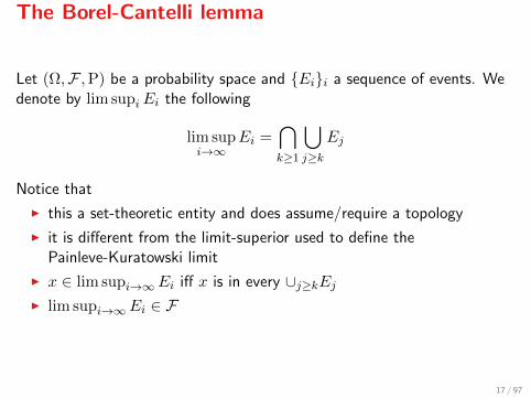
The Borel-Cantelli lemma
Let (Ω,F ,P) be a probability space and Eii a sequence of events. Wedenote by lim supiEi the following
lim supi→∞
Ei =⋂k≥1
⋃j≥k
Ej
Notice that
I this a set-theoretic entity and does assume/require a topology
I it is different from the limit-superior used to define thePainleve-Kuratowski limit
I x ∈ lim supi→∞Ei iff x is in every ∪j≥kEjI lim supi→∞Ei ∈ F
17 / 97

The Borel-Cantelli lemma
Let (Ω,F ,P) be a probability space and Eii a sequence of events. If
∞∑i=1
P[Ei] <∞,
thenP[lim sup
iEi] = 0.
18 / 97

Further reading
Excellent references:
1. S.R.S.Varadhan, Probability theory, Lecture notes, NY Univ., 2000.Available online at https://goo.gl/ygbqa3.
2. Erhan Cınlar, Probability and stochastics, Springer, 2011.
19 / 97

Summary of first section
We revised the notions
1. Probability and measure spaces, probability, conditional probability
2. Expectation and Conditional expectation
3. Stochastic process
4. Filtration and adaptation to a filtration
20 / 97

II. Markov Jump Linear Systems
1. Definition of MJLS
2. Applications
3. MJLS quirks
21 / 97

Markov processes
A Markov process is a stochastic process1 so that
P [w(k) = ω|w(0), w(1), . . . , w(k − 1)] = P [w(k) = ω|w(k − 1)] .
We assume our Markov processes are:
1. finite: w(k) is finite valued w(k) ∈ N = 1, . . . , N2. time-homogeneous: P [w(k) = j|w(k − 1) = i] = pij .
1We call stochastic process a sequence of random variables w(k) over a probabilityspace (Ω,F ,P).
22 / 97
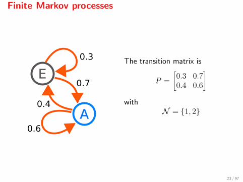
Finite Markov processes
A
E
0.3
0.7
0.6
0.4
The transition matrix is
P =
[0.3 0.70.4 0.6
]with
N = 1, 2
23 / 97
Markov jump linear systems
A (autonomous) Markov jump linear system is a dynamical system of theform
x(k + 1) = Γθ(k)x(k),
where θ(k)k is a finite time-homogeneous Markov process, x(0) = x0
and θ(0) = θ0 follows an initial distribution with P[θ(0) = ωi] = vi fori = 1, . . . , N .
24 / 97

Markov jump linear systems
Notice that x(k)k is not a Markov process, but (x(k), θ(k))k is.
25 / 97

MJLS applications
Examples
1. Power systems [Li et al. 2007; Ugrinovskii, 2005]
2. Satellite control [Meskin & Khorasani,2009]
3. Flight control [Gray, Gonzalez & Dogan, 2000]
4. Air traffic mgmt [Zhou, 2011]
5. Solar thermal receiver [Sworder & Rogers, 1983]
6. Cell growth [Horowitz et al., 2010]
7. Samuelson’s macroeconomic model [Costa et al., 1999]
8. Printer over network with random time delays [Patrinos et al., 2011]
26 / 97

MJLS quirks
Assume that some or all Γi are unstable. How will the systemtrajectories look like? Example:
Γ1 =
[2 −1
0.1 0.1
],Γ2 =
[0.2 1−0.1 2
],
and
P =
[0.1 0.90.9 0.1
].
Take x(0) = (1, 1)′ and P [w(0) = 1] = 0.5.
27 / 97
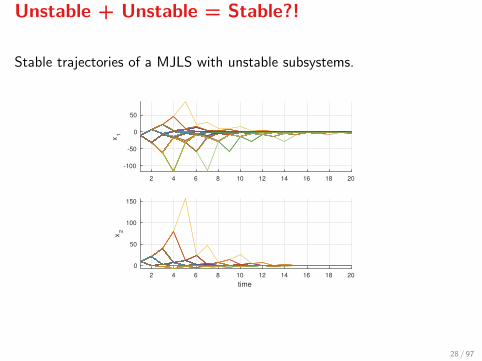
Unstable + Unstable = Stable?!
Stable trajectories of a MJLS with unstable subsystems.
2 4 6 8 10 12 14 16 18 20
x1
-100
-50
0
50
time
2 4 6 8 10 12 14 16 18 20
x2
0
50
100
150
28 / 97

MJLS quirks continued
Assume that Γi are strictly Hurwitz for all i = 1, . . . , N (all stable) – howwill the MJLS Trajectories look like? Will they all converge to zero?Example:
Γ1 =
[−0.5 2−0.5 0.5
],Γ2 =
[0.5 01 0
],
for which ρ(Γ1) = 0.866 and ρ(Γ2) = 0.5, and
P =
[0.5 0.50.5 0.5
].
Take x(0) = (1, 1)′ and P [w(0) = 1] = 0.5.
29 / 97
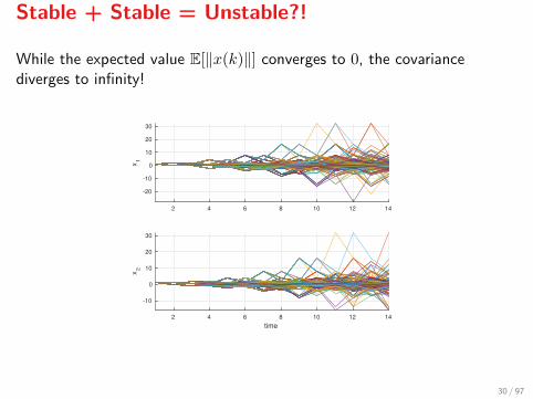
Stable + Stable = Unstable?!
While the expected value E[‖x(k)‖] converges to 0, the covariancediverges to infinity!
2 4 6 8 10 12 14
x1
-20
-10
0
10
20
30
time
2 4 6 8 10 12 14
x2
-10
0
10
20
30
30 / 97
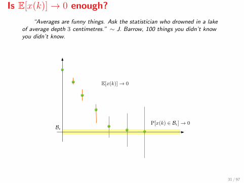
Is E[x(k)]→ 0 enough?
“Averages are funny things. Ask the statistician who drowned in a lakeof average depth 3 centimetres.” ∼ J. Barrow, 100 things you didn’t knowyou didn’t know.
31 / 97

End of second section
1. We learnt what a Markov process is
2. and the class of Markov jump linear systems
3. We then listed application of Markov jump systems
4. We realised there’s a lot to learn regarding MJLS...
32 / 97

III. MJLS dynamics
33 / 97

Questions
1. How do we model the evolution of a MJLS?
2. What definition(s) of stability apply to MJLS?
3. How do we control such a system?
34 / 97

Some definitions
For a set F ∈ F we define its characteristic function χF : Ω→ 0, 1 as
χF (ω) :=
1, if ω ∈ F0, otherwise
Then, notice that
E[x(k)] =
N∑i=1
E[x(k)χθ(k)=i]
and
E[x(k)x(k)′] =
N∑i=1
E[x(k)x(k)′χθ(k)=i]
We are going to describe the dynamics of E[x(k)] and E[x(k)x(k)′].
35 / 97

Some useful Hilbert spaces
Spaces IRn and IRn×m are Hibert spaces with inner products
〈x, y〉 := x′y, and 〈X,Y 〉 := tr(X ′Y )
We define the Hilbert space Hn,m of N -tuples of m-by-n matrices, i.e.,H = (H1, . . . ,HN ) with Hi ∈ IRm×n with the following inner product:
〈H,V 〉 :=
N∑i=1
〈Hi, Vi〉
On Hn,m we define the norms
‖H‖1 :=
N∑i=1
‖Hi‖2, and ‖H‖2 :=
N∑i=1
〈Vi, Vi〉︸ ︷︷ ︸‖Vi‖f
12
36 / 97

Some useful Hilbert spaces
We denote by Cn = L2(ω,F ,P) the space of IRn-valued random variablesy with inner product 〈y, z〉 = E[y′z] so that ‖y‖ <∞.
We call `2(Cn) the space of sequences s = s(k)k with s(k) ∈ Cn and2
‖s‖`2(Cn) :=∑k∈N‖s(k)‖2Cn <∞.
2Note that ‖s(k)‖2Cn = 〈s(k), s(k)〉Cn = E[‖s(k)‖2].
37 / 97

Some useful Hilbert spaces
Now let (Ω,F , Fkk∈N,P) be the aforementioned probability space witha filtration Fkk. We define the space Cn ⊆ `2(Cn) if for every randomprocess r ∈ Cn, r(k) is Fk-measurable, i.e., r is adapted to the filtrationFkk .
38 / 97

MJLS dynamics
We are now going to describe the dynamics of E[x(k)] and E[x(k)x(k)′].Define
qi(k) = E[x(k)χθ(k)=i
]And defining q(k) := (q1(k), . . . , q2(k)) ∈ H1,n we have
µ(k) := E[x(k)] =
N∑i=1
qi(k).
Define alsoQi(k) := E
[x(k)x(k)′χθ(k)=i
],
and let Q(k) := (Q1(k), . . . , QN (k)) ∈ Hn,n, then
Σ(k) := E[x(k)x(k)′
]=
N∑i=1
Qi(k).
39 / 97

MJLS dynamics
The mean and covariance dynamics are described by
qj(k + 1) =
N∑i=1
pijΓiqi(k)
and
Qj(k + 1) =
N∑i=1
pijΓiQi(k)Γ′i.
In what follows we will define linear operators B : q(k) 7→ q(k + 1) andT : Q(k) 7→ Q(k + 1).
40 / 97

A bound on ‖x(k)‖2
We can show that3
‖x(k)‖2 ≤ n‖Q(k)‖1,
where notice that the left hand side norm is the norm of Cn, whereas theright hand side is the 1-norm in Hn,n. What happens as Q(k)→ 0?
3In Cn = L2(Ω,F ,P, IRn) we defined the inner product 〈x, y〉 = E[x′y], so theinduced squared norm is ‖x‖2 = 〈x, x〉 = E[x′x] = E[‖x‖2].
41 / 97

Operators T and L = T ∗
We have Q(k + 1) = T [Q(k)] where T : Hn → Hn is the linear operatorT [Q] := (T1[Q], . . . , TN [Q]), with
Tj [Q] :=
N∑i=1
pijΓiQiΓ′i.
The adjoint of this operator is an operator L[Q] := (L1[Q], . . . ,LN [Q]),with
Li[Q] := ΓiEi[Q]Γi,
where Ei[Q] =∑N
i=j pijQj4.
4Use the definition, i.e., show that 〈T [Q], S〉 = 〈Q,L[S]〉 for all Q,S ∈ Hn. It isleft as an exercise to prove that T ∗ = L.
42 / 97

Operator B as a matrix
We have q(k + 1) = Bq(k), where B : IRNn → IRNn is a linear operator5
and is given by
B[q] = (P ′ ⊗ In) blkdiag(Γ1, . . . ,ΓN ) · q.
If ρ(B) < 1 then q(k)→ 0 and µ(k)→ 0, however, this does not implyQ(k)→ 0 or Σ(k)→ 0.
5Spaces IRNn and H1,n are homeomorphic (can be thought of as the same space).
43 / 97

Operator T as a matrix
For a matrix A ∈ IRm×n, A = [A1 ··· An ] we define
vec(A) := [A′1 ··· A′n ]′ ∈ IRmn.
For H ∈ Hn,m with H = (H1, . . . ,HN ), Hi ∈ IRm×n
vec(H) := [ vec(H1)′ ··· vec(Hn)′ ]′ ∈ IRNmn.
We are looking for a matrix T ∈ IRNn2×Nn2so that
vec(T [Q]) = T vec(Q)
We may verify that
T = (P ′ ⊗ In2) blkdiag(Γ′i ⊗ Γii).
44 / 97

If T is stable, then B is stable
We’ve seen that q(k)→ 0 does not imply Q(k)→ 0. However, theconverse holds true: If T is stable, then B is stable too!
ρ(T ) < 1⇒ ρ(B) < 1.
45 / 97

End of third section
1. We described the dynamics of E[x(k)] and E[x(k)x(k)′]
2. We introduced the Hilbert spaces Hn,m, Cn, `2(Cn) and Cn
3. We defined q(k) and Q(k) to study the dynamics of E[x(k)] andE[x(k)x(k)′]
4. We introduced the operators B and T using which we can study thestability properties of the dynamics of q(k) and Q(k).
46 / 97

IV. Mean square stability
47 / 97

Mean square stability
The MJLS x(k + 1) = Γθ(k)x(k) – where θ(k)k∈N is a Markov process –is mean square stable (MSS) if there is a µ and a Σ so that for anyinitial state x(0) = x0 and initial distribution of θ(0) it is
1. µ(k)→ µ,
2. Σ(k)→ Σ.
In our case, µ = 0 and Σ = 0 and #2 implies #1.
48 / 97

Why MSS?
1. It’s easy to test for
2. It implies stability of the expected state dynamics
3. It implies convergence in probability, i.e., for all ε > 0,
P[‖x(k)‖ ≥ ε]→ 0,
and further
4. It implies almost sure convergence, i.e.,
P[‖x(k)‖ → 0] = 1.
49 / 97

MSS ⇒ Convergence of E [x(k)]
MSS ⇒ Convergence of E [x(k)].
Already clear from the fact that ρ(T ) < 1⇒ ρ(B) < 1. Easy way to showit by Jensen’s inequality:
0 ≤ E [‖x(k)‖] ≤ E[‖x(k)‖2
] 12 .
BUT: Convergence of E [x(k)] ; MSS (Exercise).
50 / 97

MSS ⇔ T is stable
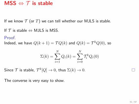
If we know T (or T ) we can tell whether our MJLS is stable.
If T is stable ⇔ MJLS is MSS.
Proof.Indeed, we have Q(k + 1) = T Q(k) and Q(k) = T kQ(0), so
Σ(k) =N∑i=1
Qi(k) =N∑i=0
T ki Qi(0)
Since T is stable, T k[Q]→ 0, thus Σ(k)→ 0.
The converse is very easy to show.
51 / 97
MSS ⇔ T is stable
If we know T (or T ) we can tell whether our MJLS is stable.
If T is stable ⇔ MJLS is MSS.
Proof.Indeed, we have Q(k + 1) = T Q(k) and Q(k) = T kQ(0), so
Σ(k) =
N∑i=1
Qi(k) =
N∑i=0
T ki Qi(0)
Since T is stable, T k[Q]→ 0, thus Σ(k)→ 0.
The converse is very easy to show.
51 / 97
MSS ⇔ MSES
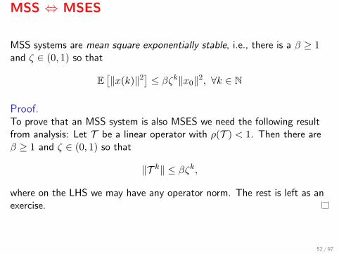
MSS systems are mean square exponentially stable, i.e., there is a β ≥ 1and ζ ∈ (0, 1) so that
E[‖x(k)‖2
]≤ βζk‖x0‖2, ∀k ∈ N
Proof.To prove that an MSS system is also MSES we need the following resultfrom analysis: Let T be a linear operator with ρ(T ) < 1. Then there areβ ≥ 1 and ζ ∈ (0, 1) so that
‖T k‖ ≤ βζk,
where on the LHS we may have any operator norm. The rest is left as anexercise.
52 / 97

Unstable + Unstable = Stable?
Two unstable modes:
Γ1 =
[2 −1
0.1 0.1
],Γ2 =
[0.2 1−0.1 2
],
with ρ(Γ1) = 1.9458 and ρ(Γ2) = 1.9426 and
P =
[0.1 0.90.9 0.1
].
but ρ(T ) = ρ(T ) = 0.6798 < 1.
53 / 97

Stable + Stable = Unstable?
Two stable modes:
Γ1 =
[−0.5 2−0.5 0.5
],Γ2 =
[0.5 01 0
],
for which ρ(Γ1) = 0.866 and ρ(Γ2) = 0.5, and
P =
[0.5 0.50.5 0.5
].
but ρ(T ) = ρ(T ) = 1.0165 > 1.
54 / 97

Stochastic stability
A MJLS is said to be stochastically stable (SS) if for all x(0) and initialdistributions for θ(0) it is
∞∑k=0
E[‖x(k)‖2
]<∞.
This is equivalent to the random process x = x(k)k being in Cn.
55 / 97

MSS ⇔ SS
A MJLS is MSS iff it is SS6.
Proof.Since E
[‖x(k)‖2
]is a sequence of `2, it converges E
[‖x(k)‖2
]→ 0. But
we have
0 ≤ E[‖x(k)‖2
]= E
[tr(x(k)x(k)′)
]= trE
[(x(k)x(k)′)
]= trQ(k)
= Σ(k),
so Σ(k)→ 0 for any x(0) and θ(0).
6This is not true for infinite Markov jump linear systems.
56 / 97

Positive (semi)definiteness
An E ∈ IRn×n is positive semidefinite (PSD) if x′Ax ≥ 0, ∀x ∈ IRn; wedenote A ≥ 0. E is positive definite (PD) if it is PSD and x′Ax = 0 onlywhen x = 0. Space of PSD (PD) matrices: Sn+ (Sn++).
It is A < B whenever B −A > 0.
Hn+: the subset of Hn so that H ∈ Hn
+ if Hi ∈ Sn+ for all i.
57 / 97

Lyapunov-like stability conditions
1. A MJLS is MSS iff for every S ∈ Hn+, S > 0, there exists a uniqueV ∈ Hn+, V > 0 such that
V − T (V ) = S.
2. A MJLS is MSS iff for some V ∈ Hn+, V > 0 it is
T (V ) < V.
Notice that V − T (V ) = S is equivalent to (id−T )V = S, which usingvon Neuman’s identity yields V =
∑∞k=0 T k [S].
58 / 97

Lyapunov-like stability conditions
A MJLS is MSS iff for every S ∈ Hn+, S > 0, there exists a uniqueV ∈ Hn+, V > 0 such that V − T (V ) = S.
Proof.Sketch: we define the following system
Y (k + 1) = L(Y (k)); Y (0) ∈ Hn+.
We need to prove that this is stable using the following Lyapunov function:
Φ(Y ) = 〈V, Y 〉
Then T = L∗ will also be stable.
59 / 97

MSS conditions using L
The first condition can also be written as
V = L(V ) + S.
and now we have
V =
∞∑k=0
Lk [S]
60 / 97

MSS conditions using V and J
We have defined the operators T and L as
Tj [Q] :=
N∑i=1
pijΓiQiΓ′i, and Li[Q] := ΓiEi[Q]Γi.
We now define the (simpler) operators V and J 7 as
Vj [Q] :=
N∑i=1
pijΓjQiΓ′j , and Ji[Q] :=
N∑j=1
Γ′jQjΓj .
Then, the MSS conditions hold also if we replace T with either V or J .
7It is V∗ = J .
61 / 97

Outlook...
These stability conditions are useful:
1. For controller design using linear matrix inequalities (LMIs)
2. To devise stabilizability and detectability tests
3. For MJLS with additive uncertainty
4. Similar conditions apply to nonlinear Markovian switching systems
62 / 97

Understanding MSS
Let x(k)k be the response of a MSS MJLS – all x(k) are randomvariables, i.e., x(k)(ω). Let θ(k)k be the corresponding sequence ofrandom parameters. Can there be a realisation θ?k so that thecorresponding state trajectory
x(k;x(0), θ(0), . . . , θ(k − 1))→∞ as k →∞ ?
Short answer: Yes! (But the probability of running into one is zero...)
63 / 97

End of fourth section
Summary:
1. MSS is a “more meaningful” (practical) stability notion than MS
2. MSS: Both µ(k) and Σ(k) converge
3. MSS ⇔ T is stable
4. MSS ⇔ MSES
5. MSS ⇔ SS
6. MSS ⇔ T V < V , and V − T V = S ∈ Hn+
64 / 97

V. Almost sure convergence
65 / 97

Zero probability for non converging x(k)
MSS ⇒ The probability that we find a realisation of x(k) that does notconverge is zero.
When is this probability zero?
If this probability is zero, do we have MSS?
66 / 97

Almost sure convergence
Under what conditions do we have x(k)→ 0 with probability one?
We say that x(k)k converges almost surely (or with probability 1) to 0if8
P(limk‖x(k)‖ = 0) = 1.
For a MJLS, MSS implies almost sure convergence – the converse is nottrue. Almost sure convergence is weaker than MSS9.
8This probability is over the space of all random processes x(k)k which satisfythe MJLS dynamics.
9This type of convergence is not induced by some metric and does not depend onany topology.
67 / 97
Almost sure convergence
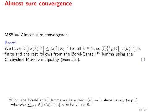
MSS ⇒ Almost sure convergence
Proof.We have E
[‖x(k)‖2
]≤ βζk‖x0‖2 for all k ∈ N, so
∑∞k=0 E
[‖x(k)‖2
]is
finite and the rest follows from the Borel-Cantelli10 lemma using theChebychev-Markov inequality (Exercise).
10From the Borel-Cantelli lemma we have that z(k) → 0 almost surely (w.p.1)whenever
∑k∈N P [‖z(k)‖ ≥ ε] <∞ for all ε > 0.
68 / 97

ASC ; MSS
ASC does not imply MSS! Example with x ∈ IR, N = 2:
Γ1 = 2.5, and Γ2 = 0.1,
and
P =
[0.5 0.50.5 0.5
]Then this is not MSS, but it converges almost surely.11
Interestingly, ρ(T ) = 3.13 (not MSS), but also ρ(B) = 1.3 (not MS)!
11See: Fang et al. 1994.
69 / 97

ASC ; MSS
k
5 10 15 20 25
E[x
(k)]
50
100
150
200
250
300
350
400
450
500
70 / 97

Understanding ASC
k
5 10 15 20 25
x(k
)
0
500
1000
1500
2000
2500
3000
71 / 97

Understanding ASC
7
6
5
4
k
3
2
1250
200x
150100
500
1
0.8
0.6
0.4
0.2
0
P[x
(k)=
x]
72 / 97

Understanding ASC
There is zero probability that we find a realisation of x(k)kwhich does not converge to 0.
73 / 97

Understanding ASC
k
0 20 40 60 80 100
x1(k
)
0
0.2
0.4
0.6
0.8
1
74 / 97

Understanding ASC
k
0 20 40 60 80 100
x2(k
)
0
0.2
0.4
0.6
0.8
1
75 / 97

Understanding ASC
k
0 20 40 60 80 100
x3(k
)
0
200
400
600
800
1000
1200
1400
1600
76 / 97

Modes of convergences
77 / 97
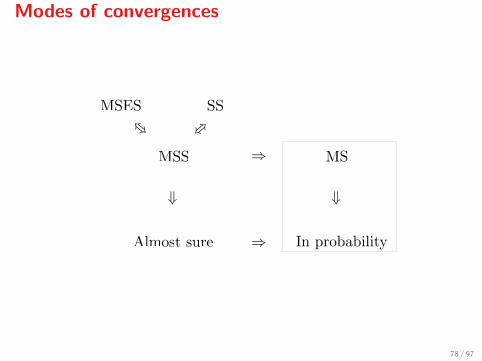
Modes of convergences
78 / 97
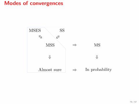
Modes of convergences
79 / 97

Modes of convergences
80 / 97

Modes of convergences
81 / 97

Question
Under what conditions ‖x(k)‖ → 0 almost surely?
82 / 97

Interlude: Ergodicity
A finite Markov jump process θ(k) is called ergodic if from every modei ∈ N we can move to any mode j ∈ N (not necessarily in one step).
Let πi(k) := P [θ(k) = i]. Under the ergodicity assumption, there is aprobability distribution π = π1, . . . , πN, πi > 0, such that
πi(k)→ πi.
And we can compute π solving12
P ′π = π.
12For details, I recommend the lecture notes of J. Gravner (UC Davis) on “intro-ductory probability”.
83 / 97

Take ν pos. integer and let
θ(k) = (θ(kν + ν − 1), . . . , θ(kν)) ∈ N ν
be a Markov chain. Take ι = (iν−1, . . . , ι0) and τ = (jν−1, . . . , j0) ∈ N ν .The transition probabilities of θ(k) are
P[θ(k + 1) = τ | θ(k) = ι
]= piν−1j0pj0j1 . . . pjν−1jν−1 .
We have P[θ(k) = τ
]= P [θ(kν) = j0] pj0j1 . . . pjν−1jν−1 and as k →∞
this converges toπ := πj0pj0j1 . . . pjν−1jν−1 .
84 / 97

Conditions for ASC
TheoremLet Γι := Γiν−1 . . .Γi0 . If there is ν pos. integer. s.t.∏
ι∈N ν‖Γι‖πι < 1,
then x(k)→ 0 a.s.; ‖ · ‖ can be any matrix norm.
85 / 97

Exercises
Exercise 1. Determine a system with n = 2, N = 2 which is ASC but notMSS.
Exercise 2. Show that a system with n = 1, N = 2, and θ(k): i.i.d. withπ1 = π2 = 0.5 and Γ1 = α, Γ2 = β is ASC if and only if |αβ| < 1.
Exercise 3. For a stochastic process x(k)k we know that E[x(k)]→ 0.Is the process ASC?
86 / 97

End of fifth section
Summary:
1. Almost sure convergence is weaker than MSS
2. ASC is convergence w.p.1.
3. ASC implies convergence in probability
4. The notion of almost sure convergence is not induced by a topology
5. A system can be ASC but not MSS or even MS
6. When the Markov process is ergodic, πi(k) converges
87 / 97

VI. Feedback stabilisation
88 / 97
Feedback stabilisation
We need to design a mean square stabilising controller for the system
x(k + 1) = Aθ(k)x(k) +Bθ(k)u(k).
We assume x(k), θ(k) are measured and the controller has the form
u(k) = κ(θ(k), x(k)) = Fθ(k)x(k),
so the closed-loop MJLS is
x(k + 1) = (Aθ(k) +Bθ(k)Fθ(k))x(k).
89 / 97

Feedback stabilisation
The closed-loop system is MSS if there is V ∈ Hn+ so that T (V ) < V , i.e.,
for all j ∈ N
Vj −N∑i=1
pij(Aθ(k) +Bθ(k)Fθ(k))Vi(Aθ(k) +Bθ(k)Fθ(k))′ > 0
which can be written as a LMI using the Schur complement lemma(Exercise).
90 / 97

Feedback stabilisation
Comments:
1. We have one controller for each mode.
2. For each i ∈ N , we didn’t select Fi so as to stabilise (Ai, Bi).
3. Had we done that, would the closed-loop MJLS be MSS?
4. In practice, θ(k) may not be known exactly.
91 / 97

Stabilisation with inexact knowledge of θ(k)
Assume θ(k) is not available at time k, but we have an estimateθ(k) ∈ N (which defines a random process). Then,
u(k) = Fθ(k)x(k),
and the closed-loop MJLS will be
x(k + 1) = (Aθ(k) +Bθ(k)Fθ(k))x(k).
92 / 97

Stabilisation with inexact knowledge of θ(k)
We define the following filtration Mkk∈N with M0 = F0 and Mk is theσ-algebra generated by
x(0), θ(0), x(1), θ(1), θ(0), . . . , x(k), θ(k), θ(k − 1).
We assume that
P[θ(k) = s |Mk
]= P
[θ(k) = s | θ(k)
]=: ρθ(k)s.
This means that
ρis = probability that θ(k) = i while we estimated θ(k) = s
andρis = probability of success: θ(k) = θ(k) = i
93 / 97

Stabilisation with inexact knowledge of θ(k)
Letp = min
iρii.
Let T : Hn → Hn be defined as before with Γi = Ai +BiFi. Since T isstable, there are β ≥ 1 and ζ ∈ (0, 1) s.t.13
‖T k‖1 ≤ βζk.
Finally, let
c0 := max‖Ai +BiFs‖2, i, s ∈ N, i 6= s, ρis > 0
.
13Question: How do we determine those parameters? Can you give an examplewhen N = 1 and N = 2?
94 / 97

Stabilisation with inexact knowledge of θ(k)
MSS condition:
p > 1− 1− ζc0β
.
Proof.The proof is a bit lengthy and can be found in the book of Costa et al.(Lemma 3.44). Sketch: We show that
0 ≤ Qj(k + 1) ≤ Tj [Q(k)] + Sj [Q(k)],
where S : Hn → Hn is such that ‖S‖1 ≤ c0(1− p).
95 / 97

Further reading
1. O.L.V. Costa, M.D. Fragoso and R.P. Marques, Discrete-time Markov Jump LinearSystems, Springer 2005.
2. Y. Fang and K.A. Loparo, Stochastic Stability of Jump Linear Systems, IEEETrans. Aut. Contr. 47(7), pp. 1204–1208, 2002.
96 / 97

References for ASC
1. Y. Fang, K.A. Loparo, and X. Feng. Almost sure and δ-moment stability of jumplinear systems. International Journal of Control, 59:1281–1307, 1994.
2. O. L. V. Costa and M. D. Fragoso. Stability results for discrete-time linear systemswith Markovian jumping parameters. Journal of Mathematical Analysis andApplications, 179:154–178, 1993.
3. J. B. R. do Val, C. Nespoli, and Y. R. Z. Caceres. Stochastic stability forMarkovian jump linear systems associated with a finite number of jump times.Jounal of Mathematical Analysis and Applications, 285:551–563, 2003.
4. Y. Fang. A new general sufficient condition for almost sure stability of jump linearsystems. IEEE Transactions on Automatic Control, 42:378–382, 1997.
5. Z. G. Li, Y. C. Soh, and C. Y. Wen. Sufficient conditions for almost sure stabilityof jump linear systems. IEEE Transactions on Automatic Control, 45:1325–1329,2000.
6. M. Mariton. Almost sure and moments stability of jump linear systems. Systemsand Control Letters, 30:1145–1147, 1985.
97 / 97


![Markov Jump Linear Quadratic Dynamic Programming · 2021. 6. 24. · d_vals=[1., 1.]): """ Construct matrices that map the problem described in example 1 into a Markov jump linear](https://static.fdocuments.in/doc/165x107/614025fae59fcb3c636a4f98/markov-jump-linear-quadratic-dynamic-programming-2021-6-24-dvals1-1.jpg)
