Markov Chain Sampling Methods for

Dirichlet Process Mixture Models

Radford M. Neal, University of Toronto, Ontario, Canada

Presented by Colin DeLong

OutlineIntroductionDirichlet process mixture modelsGibbs sampling w/ conjugate priors

Algorithms 1, 2, and 3Methods for handling non-conjugate priors

Algorithm 4 Metropolis-Hastings and partial Gibbs

Algorithms 5, 6, and 7Gibbs sampling w/ auxiliary parameters

Algorithm 8Experiments (well, one)

IntroductionSome problems are more accurately represented with non-conjugate priors

Audio interpolation (Godsill & Rayner, 1995)Climatology opinion quantification (Al-Awadhi & Garthwaite, 2001)Financial risk assessment (Siu & Yang, 1999)

Non-conjugate priors + Gibbs = headache.Update integrals are nasty to compute

Solution? Metropolis-Hastings + partial Gibbs.

Dirichlet process mixture models

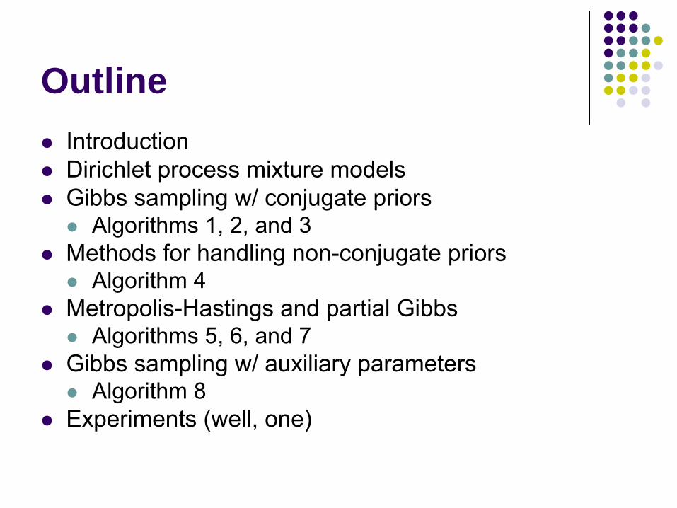
Basic ideaGiven data y1,…,yn ind. drawn from an unknown distribution (yimay be multivariate)Model the unknown distribution as being drawn from of a mixture of distributions F(θ), w/ mixing distribution over θ being G.Let prior for G be a Dirichlet process w/ concentration parameter α and base distribution G0.Then you have:

yi

Dirichlet process mixture models

Integrate over G in previous model, giving a representation of the prior distribution of θi in terms of previous θ’s:

δ(θ) is distribution concentrated at point θ.You might notice the “Chinese Restaurant Process” at work here

Dirichlet process mixture models

You can also get here by letting K (# of components) go to ∞…

ci is the latent class associated with yiThe parameters φc determine the distribution of observations from c

Dirichlet process mixture models

Integrate over mixing proportions pc to write prior of ci as follows:

Where ni,c is the number of cj for j < i equal to c. Letting K go to ∞, we get ci’s prior as:

Gibbs sampling w/ conjugate priors

Exact computation of posterior for DP mixture models not feasible, so use Monte Carlo approachesSample from posterior of θ1,…,θn by simulating a Markov chain with this posterior as its equilibrium distributionGibbs sampling is the natural approach here for conjugate priors3 main ways of doing this

Algorithm 1 (Escobar, 1994)

Where Hi is the posterior for θ based on the prior G0 and yi, having likelihood F(yi, θ) and:

Convergence may be slow due to groups of observations that are highly probably to be associated with the same θ

Algorithm 2 (West, Muller, & Escobar, 1994)

Algorithm 3 (Neal, 1992)

Methods for handling non- conjugate priors

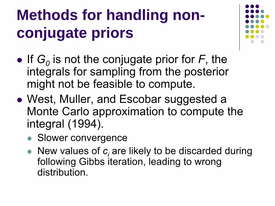
If G0 is not the conjugate prior for F, the integrals for sampling from the posterior might not be feasible to compute.West, Muller, and Escobar suggested a Monte Carlo approximation to compute the integral (1994).

Slower convergenceNew values of ci are likely to be discarded during following Gibbs iteration, leading to wrong distribution.

Algorithm 4 (MacEachern & Muller, 1998)

Problem with Algorithm 4

Algorithm 4 has a problem in that assigning cito a new component is reduced by a factor of k- + 1.However, something similar without this problem is possible.

Metropolis-Hastings and partial Gibbs

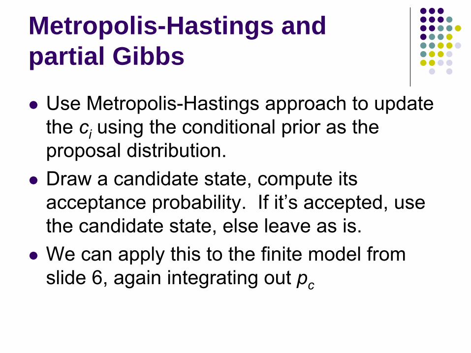
Use Metropolis-Hastings approach to update the ci using the conditional prior as the proposal distribution.Draw a candidate state, compute its acceptance probability. If it’s accepted, use the candidate state, else leave as is.We can apply this to the finite model from slide 6, again integrating out pc

Algorithm 5 (Neal, 1998)

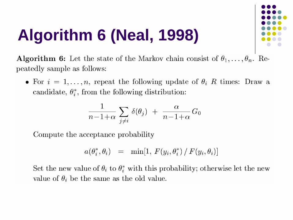
Algorithm 6 (Neal, 1998)

Algorithm 7 (Neal, 1998)

Gibbs sampling w/ auxiliary parameters

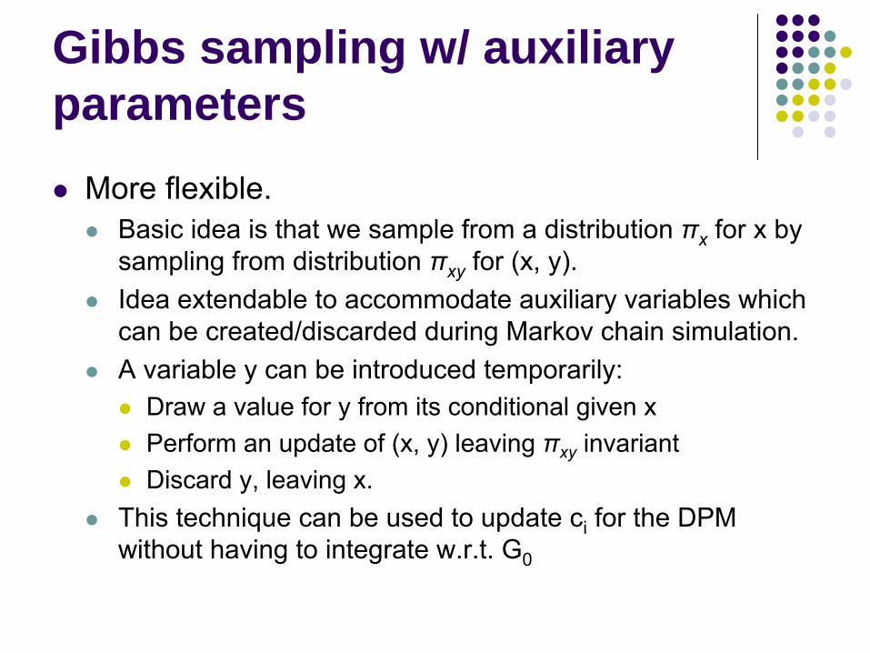
More flexible.Basic idea is that we sample from a distribution πx for x by sampling from distribution πxy for (x, y).Idea extendable to accommodate auxiliary variables which can be created/discarded during Markov chain simulation.A variable y can be introduced temporarily:

Draw a value for y from its conditional given xPerform an update of (x, y) leaving πxy invariantDiscard y, leaving x.

This technique can be used to update ci for the DPM without having to integrate w.r.t. G0

Algorithm 8 (Neal, 1998)

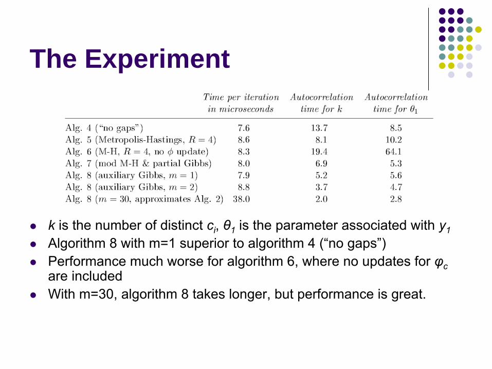
The Experiment

k is the number of distinct ci, θ1 is the parameter associated with y1Algorithm 8 with m=1 superior to algorithm 4 (“no gaps”)Performance much worse for algorithm 6, where no updates for φcare includedWith m=30, algorithm 8 takes longer, but performance is great.