Markov Chain Monte Carlo Simulations and TheirStatistical Analysis – An Overview

Bernd Berg

FSU, August 30, 2005

Content

1. Statistics as needed

2. Markov Chain Monte Carlo (MC)

3. Statistical Analysis of MC Data and Advanced MC.

Link to computer code at www.hep.fsu.edu/˜ berg .

1

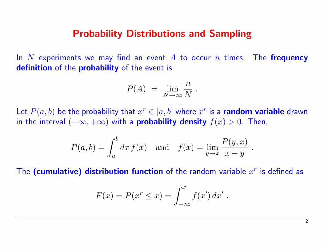
Probability Distributions and Sampling

In N experiments we may find an event A to occur n times. The frequencydefinition of the probability of the event is

P (A) = limN→∞

n

N.

Let P (a, b) be the probability that xr ∈ [a, b] where xr is a random variable drawnin the interval (−∞,+∞) with a probability density f(x) > 0. Then,

P (a, b) =∫ b

a

dx f(x) and f(x) = limy→x

P (y, x)x− y

.

The (cumulative) distribution function of the random variable xr is defined as

F (x) = P (xr ≤ x) =∫ x

−∞f(x′) dx′ .

2

For uniform probability distribution between [0, 1),

u(x) ={ 1 for 0 ≤ x < 1;

0 elsewhere.

The corresponding distribution function is

U(x) =∫ x

−∞u(x′) dx′ =

{ 0 for x < 0;x for 0 ≤ x ≤ 1;1 for x > 1.

It allows for the construction of general probability distributions. Let

y = F (x) =∫ x

−∞f(x′) dx′ .

For yr being a uniformly distributed random variable in [0, 1)

xr = F−1(yr) is then distributed according to the probability density f(x) .

3

Example

Mapping of the uniform to the Cauchy distribution.

0

0.2

0.4

0.6

0.8

1

-10 -5 0 5 10

Uni

form

yr

Cauchy xr

4

Pseudo Random Numbers and Computer Code

It is sufficient to generate uniform (pseudo) random numbers. Control your randomnumber generator! Therefore, a portable, well-tested generator should be choosen.My code supplies a generator by Marsaglia and collaborators whith an approximateperiod of 2110. How to get it? Download STMC.tgz which unfolds under (Linux)

tar -zxvf STMC.tgzinto the directory structure shown below.

STMC

ForProgAssignments ForLib ForProc Work

a0102_02 a0102_03 ... ... a0103_01 ... ...

5

Routines:rmaset.f sets the initial state of the random number generator.ranmar.f provides one random number per call (function version rmafun.f).rmasave.f saves the final state of the generator.

Initial seeds

−1801 ≤ iseed1 ≤ 29527 and − 9373 ≤ iseed2 ≤ 20708 .

give independent series (useful for parallel processing).

Illustration: Assignment a0102 02.

RANMAR INITIALIZED. MARSAGLIA CONTINUATION.idat, xr = 1 0.116391063 idat, xr = 1 0.495856345idat, xr = 2 0.96484679 idat, xr = 2 0.577386141idat, xr = 3 0.882970393 idat, xr = 3 0.942340136idat, xr = 4 0.420486867 idat, xr = 4 0.243162394extra xr = 0.495856345 extra xr = 0.550126791

6

Confidence Intervals and Sorting

One defines q-tiles (also quantiles or fractiles) xq of a distribution function by

F (xq) = q .

An example is the median x12. The probability content of the confidence interval

[xq, x1−q] is p = 1− 2q .

Example: Gaussian or normal distribution of variance σ2 :

[−nσ,+nσ] ⇒ p = 0.6827 for n = 1, p = 0.9545 for n = 2 .

The peaked distribution function

Fq(x) ={

F (x) for F (x) ≤ 12,

1− F (x) for F (x) > 12.

7

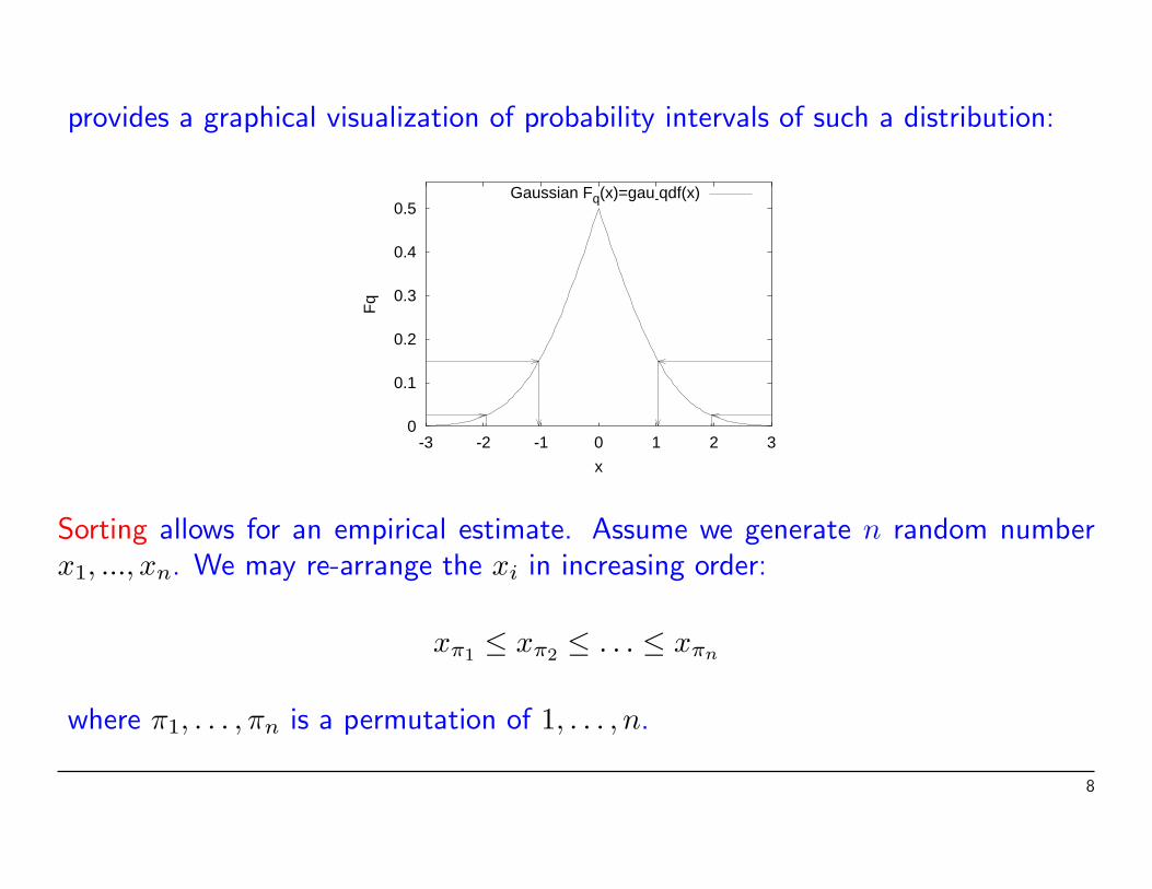
provides a graphical visualization of probability intervals of such a distribution:

0

0.1

0.2

0.3

0.4

0.5

-3 -2 -1 0 1 2 3

Fq

x

Gaussian Fq(x)=gau-qdf(x)

Sorting allows for an empirical estimate. Assume we generate n random numberx1, ..., xn. We may re-arrange the xi in increasing order:

xπ1 ≤ xπ2 ≤ . . . ≤ xπn

where π1, . . . , πn is a permutation of 1, . . . , n.

8

An estimator for the distribution function F (x) is then the empirical distributionfunction

F (x) =i

nfor xπi

≤ x < xπi+1, i = 0, 1, . . . , n− 1, n

with the definitions xπ0 = −∞ and xπn+1 = +∞. To calculate F (x) one needsan efficient way to sort n data values in ascending (or descending) order. In theSTMC package this is provided by a heapsort routine, which arrives at the resultsin O(n log2 n) steps.

Example: Gaussian distribution in assignment a0106 02 (200 and 20,000 data).

Central Limit Theorem: Convergence of the Sample Mean

Gaussian σ2(xr) =σ2(xr)

Nfor x =

1N

N∑i=1

xi .

9

Binning

We group NDAT data into NBINS bins, where each binned data point is the arithmeticaverage of

NBIN = [NDAT/NBINS] (Fortran integer division.)

original data points. Should not be confused with histogramming! Preferably NDATis a multiple of NBINS. The purpose of the binning procedure is twofold:

1. When the the central limit theorem applies, the binned data will becomepractically Gaussian when NBIN is large enough. This allows to apply Gaussianerror analysis methods even when the original are not Gaussian.

2. When data are generated by a Markov process subsequent events are correlated.For binned data these autocorrelations are reduced and can be neglected, onceNBIN is sufficiently large.

10

Example:

0

1

2

3

4

5

6

7

0.25 0.3 0.35 0.4 0.45 0.5 0.55 0.6 0.65 0.7 0.75

H

xr

Normal distributionBinned data

Figure 1: Comparison of a histogram of 500 binned data with the normal distributionp(120/π) exp[−120 (x − 1/2)2]. Each binned data point is the average of 20 uniformly

distributed random numbers. Assignment a0108 02.

11

Gaussian Difference Test

One is often faced with comparing two different empirical estimates of some mean.How large must D = x− y be in order to indicate a real difference? The quotient

dr = Dr/σD , σ2D = σ2

x + σ2y

is normally distributed with expectation zero and variance one. The likelihoodthat the observed difference |x− y| is due to chance is defined to be

Q = 1− P (|dr| ≤ d) = 2G0(−d) = 1− erf(d/√

2)

.

If the assumption is correct, then Q is a uniformly distributed random variable inthe range [0, 1). Examples: (interactive in ForProc/Gau dif/)

x1 ± σx1 1.0± 0.1 1.0± 0.1 1.0± 0.1 1.0± 0.05 1.000± 0.025x2 ± σx2 1.2± 0.2 1.2± 0.1 1.2± 0.0 1.2± 0.00 1.200± 0.025

Q 0.37 0.16 0.046 0.000063 0.15× 10−7

12

Gaussian Error Analysis for Small Samples:

Gosset’s Student Distribution and the Student Difference Test.

The Error of the Error Bar:

χ2 Distribution and the Variance Ratio Test (F-Test).

The Jackknife Approach:

Jackknife estimators correct for the bias and the error of the bias. If there is notbias, their results are identical with the conventional error analysis. As the extraeffort of using Jacknife routines is minimal, they should be the standard of erroranalysis.

Bias problems occur when one estimates a non-linear function of a mean x:

f = f(x) .

13

Jacknife estimators of the function are then defined by

fJ

=1N

N∑i=1

fJi with fJ

i = f(xJi ) and xJ

i =1

N − 1

∑k 6=i

xk .

The estimator for the variance is

s2J(f

J) =

N − 1N

N∑i=1

(fJi − f

J)2 .

Straightforward algebra shows that in the unbiased case the jackknife variancereduces to the normal variance. Of order N (not N2) operations are needed toconstruct the jackknife averages xJ

i , i = 1, . . . , N from the original data.

Determination of Parameters (Fitting):

Levenberg-Marquardt approach besides simple linear regression.

14

Statistical Physics and Markov Chain Monte Carlo Simulations

MC simulations of systems described by the Gibbs canonical ensemble aim atcalculating estimators of physical observables at a temperature T . In the followingwe consider the calculation of the expectation value of an observable O. All systemson a computer are discrete, because a finite word length has to be used. Hence,

O = O(β) = 〈O〉 = Z−1K∑

k=1

O(k) e−β E(k)

where Z = Z(β) =K∑

k=1

e−β E(k)

is the partition function. The index k = 1, . . . ,K labels all configurations (ormicrostates) of the system, and E(k) is the (internal) energy of configuration k.

15

In the following I use Potts models on d-dimensional cubic lattices with periodicboundary conditions. Without being overly complicated, these models allow toillustrate essential features we are interested in. We define the energy of the systemby

E(k)0 = −2

∑<ij>

δ(q(k)i , q

(k)j ) +

2 d N

qwith δ(qi, qj) =

{1 for qi = qj

0 for qi 6= qj.

The sum < ij > is over the nearest neighbor lattice sites and the Potts spins

or states of q(k)i take the values 1, . . . , q. For the energy per spin the notation is

es = E/N and our normalization is chosen so that es agrees for q = 2 with theconventional Ising model definition. For the 2d Potts models a number of exactresults are known, e.g.,

βc =1Tc

=12

ln(1 +√

q) = βPottsc , ec

0s = Ec0/N =

4q− 2− 2/

√q .

The phase transition is second order for q ≤ 4 and first order for q ≥ 5.

16

Markov Chain Monte Carlo

A Markov chain allows to generate configurations k with probability

P(k)B = cB w

(k)B = cB e−βE(k)

, cB constant .

The state vector (P (k)B ), for which the configurations are the vector indices,

is called Boltzmann state. A Markov chain is a simple dynamic process, whichgenerates configuration kn+1 stochastically from configuration kn. Let the transitionprobability to create the configuration l in one step from k be given by W (l)(k) =W [k → l]. Then, the transition matrix

W =(W (l)(k)

)defines the Markov process. Note, that this matrix is a very big and never stored

in the computer. The matrix achieves our goal and generates configurations withthe desired probabilities, when it satisfies the following properties:

17

(i) Ergodicity:

e−βE(k)> 0 and e−βE(l)

> 0 imply :an integer number n > 0 exists so that (Wn)(l)(k) > 0 holds.

(ii) Normalization: ∑l

W (l)(k) = 1 .

(iii) Balance: ∑k

W (l)(k) e−βE(k)= e−βE(l)

.

Balance means: The Boltzmann state is an eigenvector with eigenvalue 1 ofthe matrix W = (W (l)(k)).

With that we have replaced the canonical ensemble average by a time average overan artificial dynamics and one distinguishes dynamical universality classes.

18

The Metropolis Algorithm

Detailed balance still does not uniquely fix the transition probabilities W (l)(k). TheMetropolis algorithm is a popular choice can be used whenever one knows how tocalculate the energy of a configuration. Given a configuration k, the Metropolisalgorithm proposes a configuration l with probability

f(l, k) = f(k, l) normalized to∑

l

f(l, k) = 1 .

The new configuration l is accepted with probability

w(l)(k) = min

[1,

P(l)B

P(k)B

]=

{1 for E(l) < E(k)

e−β(E(l)−E(k)) for E(l) > E(k).

If the new configuration is rejected, the old configuration has to be counted again.

19

The Heatbath algorithm

The heat bath algorithm chooses a spin qi directly with the local Boltzmanndistribution defined by its nearest neighbors

PB(qi) = const e−β E(qi) .

As many Metropolis hits (on the same spin) are needed to reach this distribution,the heatbath is more efficient than the Metropolis algorithm. However, itmodels more complicated than Potts models the calculation of the local heatbathprobabilities is often too involved to make it a viable alternative.

Start and equilibration

Initially we have to start with a microstate which may be far off the Boltzmanndistribution. Although the weight of states decreases with 1/n where n is the stepsof the Markov process, one should exclude the initial states from the equilibriumstatistics. Many ways to generate start configurations exist, e.g.,

20

1. A random configuration corresponding to β = 0.

2. An ordered configuration for which all Potts spins take on the same q-value.

Examples: (assignments a0303 01 and a0303 05)

-2

-1.5

-1

-0.5

0

0 50 100 150 200

e 0s

Sweeps

Random StartOrdered Start

Exact

0.1

0.2

0.3

0.4

0.5

0.6

0.7

0.8

0.9

1

0 50 100 150 200ac

tSweeps

Ordered starts

Disordered starts

Metropolis 1-hitMetropolis 2-hit

Heat Bath

Figure 2: Initial time series of 200 sweeps each on a 80 × 80 lattice. Left: Metropolis for a 2d

Ising model at β = 0.4. Right: q = 10 Potts model at β = 0.62.

21

Consistency Checks

For the 2d Ising model we can test against the exact finite lattice results ofFerdinand and Fisher. We simulate a 202 lattice at β = 0.4 using 10 000 sweeps forreaching equilibrium 64 bins of 5 000 sweeps for measurement (a careful justificationis given later). We find (assignment a0303 06)

e0s = −1.1172 (14) (Metropolis) versus es = −1.117834 (exact) .

The Gaussian difference test gives a perfectly admissible value Q = 0.65 .

For the 2d 10-state Potts model at β = 0.62 we test our Metropolis versus ourheat bath code on a 20× 20 lattice to find (assignment a0303 08)

actm = 0.321772 (75) (Metropolis) versus actm = 0.321661 (70) (heat bath)

and Q = 0.28 for the Gaussian difference test. Another perfectly admissible value.

22

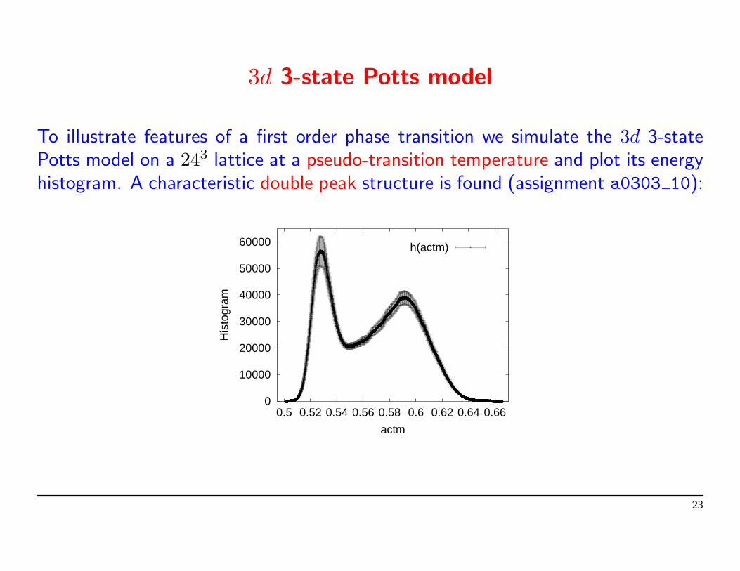
3d 3-state Potts model

To illustrate features of a first order phase transition we simulate the 3d 3-statePotts model on a 243 lattice at a pseudo-transition temperature and plot its energyhistogram. A characteristic double peak structure is found (assignment a0303 10):

0

10000

20000

30000

40000

50000

60000

0.5 0.52 0.54 0.56 0.58 0.6 0.62 0.64 0.66

His

togr

am

actm

h(actm)

23

Self-Averaging Illustration for the 2d Heisenberg model

We compare the peaked distribution function of a mean energy density perlink for different lattice sizes. The property of self-averaging is observed: Thelarger the lattice, the smaller the confidence range. The other way round, thepeaked distribution function is very well suited to exhibit observables for whichself-averaging does not work, as for instance encountered in spin glass simulations.

0

0.1

0.2

0.3

0.4

0.5

0.36 0.38 0.4 0.42 0.44 0.46 0.48 0.5

Fq

actm

L=20L=34L=60

L=100

Figure 3: O(3) σ-model at β = 1.1 (assignments a0304 06 and a0304 08).

24

Statistical Errors of Markov Chain MC Data

A typical MC simulation falls into two parts:

1. Equilibration without measurements.

2. Production with measurements.

Rule of thumb (for long calculations): Do not spend more than 50% of yourCPU time on measurements!

Autocorrelations

We like to estimate the expectation value f of some physical observable. Weassume that the system has reached equilibrium. How many MC sweeps are neededto estimate f with some desired accuracy? To answer this question, one has tounderstand the autocorrelations within the Markov chain.

25

Given is a time series of measurements fi, i = 1, . . . , N . With the notationt = |i− j| the autocorrelation function of the mean f is defined by

C(t) = Cij = 〈 (fi − 〈fi〉) (fj − 〈fj〉) 〉 = 〈fifj〉 − 〈fi〉 〈fj〉 = 〈f0ft〉 − f 2

Some algebra shows that the variance of the estimator f for the mean and theautocorrelation functions are related by

σ2(f) =σ2(f)

N

[1 + 2

N−1∑t=1

(1− t

N

)c(t)

]with c(t) =

C(t)

C(0).

This equation ought to be compared with the corresponding equation foruncorrelated random variables σ2(f) = σ2(f)/N . The difference is the factorin the bracket which defines the integrated autocorrelation time as

τint = limN→∞

[1 + 2

N−1∑t=1

(1− t

N

)c(t)

].

26

Self-consistent versus reasonable error analysis

The calculation of the integrated autocorrelation provides a self-consistent erroranalysis. But in practice this is often out of reach.

According to the Student distribution about twenty independent data aresufficient to estimate mean values reliably, while the error of the error bar the χ2

distribution implies that about one thousand are needed for an estimate of theintegrated autocorrelation time with 10% accuracy on the two σ confidence level.

In practice, one may rely on the binning method with a fixed number of ≥ 16bins. How do we know then that the statistics has become large enough? Therecan be indirect arguments like finite size scale extrapolations, which suggest thatthe integrated autocorrelation time is (much) smaller than the achieved bin length.This is no longer self-consistent, but a reasonable error analysis.

27

Comparison of Markov chain MC algorithms

The d = 2 Ising model at the critical temperature

0

500

1000

1500

2000

2500

0 1000 2000 3000 4000 5000 6000 7000 8000

τ int

t

L=160 ts1L= 80 ts1L= 40 ts1L= 20 ts1

Figure 4: One-hit Metropolis algorithm with sequential updating: critical slowingdown, τint ∼ Lz where z ≈ 2.17 is the dynamical critical exponent (assignmenta0402 02 D).

28

Another MC dynamics, Swendsen-Wang (SW) and Wolff (W) cluster algorithm:

2

4

6

8

10

12

14

0 10 20 30 40 50 60

τ int

t

SW L=160SW L= 80SW L= 40SW L= 20W L=160W L= 80W L= 40W L= 20

Figure 5: Estimates of integrated autocorrelation times from simulations of thed = 2 Ising model at the critical temperature (assignment a0503 05).

29

Simulations of the Multicanonical Ensemble

One of the questions which ought to be addressed before performing a largescale computer simulation is “What are suitable weight factors for the problem athand?” So far we used the Boltzmann weights as this appears natural for simulatingthe Gibbs ensemble. However, a broader view of the issue is appropriate.

Conventional simulations can by re-weighting techniques only be extrapolatedto a vicinity of the simulation temperature. For multicanonical simulations this isdifferent. A single simulation allows to obtain equilibrium properties of the Gibbsensemble over a range of temperatures. Of particular interest are two situationsfor which canonical simulations do not provide the appropriate implementation ofimportance sampling:

1. The physically important configurations are rare in the canonical ensemble.

2. A rugged free energy landscape makes the physically important configurationsdifficult to reach.

30

Multicanonical simulations sample, in an appropriate energy range, with anapproximation to the weights

wmu(k) = wmu(E(k)) = e−b(E(k)) E(k)+a(E(k)) =1

n(E(k))

where n(E) is the spectral density. The function b(E) defines the inversemicrocanonical temperature and a(E) the dimensionless, microcanonical freeenergy. The function b(E) has a relatively smooth dependence on its arguments,which makes it a useful quantity when dealing with the weight factors. Themulticanonical method requires two steps:

1. Obtain a working estimate the weights. Working estimate means that theapproximation has to be good enough so that the simulation covers the desiredeneryg or temperature range.

2. Perform a Markov chain MC simulation with the fixed weights. The thusgenerated configurations constitute the multicanonical ensemble.

31

Re-Weighting to the Canonical Ensemble

Given the multicanonical time series, where i = 1, . . . , n labels the generatedconfigurations. The formula

O =∑n

i=1O(i) exp[−β E(i) + b(E(i)) E(i) − a(E(i))

]∑ni=1 exp

[−β E(i) + b(E(i)) E(i) − a(E(i))

] .

replaces the multicanonical weighting of the simulation by the Boltzmann factor.The denominator differs from the partition function Z by a constant factor whichdrops out (for discrete systems this simplifies for functions of the energy usinghistograms). The computer implementation of these equations requires care and aJackknife analysis with logarithmic coding relying on the formula

lnC = max (lnA, lnB) + ln{1 + exp [−| lnA− lnB|]}

ought to be used.

32

Energy and Specific Heat Calculation

Multicanonical data for the energy per spin (with jackknife errors) of the 2d Isingmodel on a 20 × 20 lattice are produced in assignment a0501 01 and comparedwith the exact results of Ferdinand and Fisher in assignment a0501 03. Results:

-2

-1.5

-1

-0.5

0

0 0.1 0.2 0.3 0.4 0.5 0.6

<e 0

s>

β

Energy per spin <e0s>Multicanonical data

33

The same numerical data allow to calculate the specific heat defined by

C =d E

d T= β2

(〈E2〉 − 〈E〉2

).

0

0.2

0.4

0.6

0.8

1

1.2

1.4

1.6

1.8

0 0.2 0.4 0.6 0.8 1

C/N

β

Specific heat per spin

34

Free Energy and Entropy Calculation

At β = 0 the Potts partition function is Z = qN . Therefore, multicanonicalsimulations allow for proper normalization of the partition function, if β = 0is included in the temperature range. Example: Entropies from multicanonicalsimulations of the The 2d Ising and 10-state Potts models on a 20 × 20 lattice(assignment a0501 03 for Ising and a0501 05 for 10-state Potts).

0

0.1

0.2

0.3

0.4

0.5

0.6

0.7

0.8

0 0.2 0.4 0.6 0.8 1

s

β

Ising10-state Potts

35

Summary

• We considered Statistics, Markov Chain Monte Carlo simulations, the StatisticalAnalysis of Markov chain data and, finally, Multicanonical Sampling.

• It is a strength of computer simulations that one can generate artificial (notrealized by nature) ensembles, which enhance the probabilities of rare events onmay be interested in, or speed up the dynamics.

• Each method comes with its entire computer code.

36